processes in discrete and continuous time · wavelets analysis and in digital signal processing,...

PROCESSES IN DISCRETE AND CONTINUOUS TIME

by D.S.G. POLLOCKUniversity of Leicester

I wish to discuss the relationship between discrete-time linear stochastic models and theircontinuous-time counterparts.

The original proponents of continuous-time econometrics were concerned with structuraleconometric models.

The identification of the equations requires a priori information, usually in the form ofexclusion restrictions, which indicate that some of the system’s variables are absent fromsome of its equations.

It was observed that, if such restrictions were valid for continuous-time models, then,on account of the feedback occurring in the time between successive observations, therestrictions would not be valid in discrete-time models.

Hence the requirement to model in continuous time.

My principal interest in the discrete–continuous relationship has a different motivation.I am interested in wavelets analysis and in digital signal processing, where the discrete–continuous correspondence in an essential feature.

1

POLLOCK: Processes in Discrete and Continuous Time

A Misunderstanding of the Discrete–Continuous Relationship

There is a common misunderstanding that can be illustrated by quoting a passage fromthe Palgrave handbook on Macroeconometrics and Time Series Analysis:

“A model built in continuous time can include discrete delays and discontinuities.But, only if all of the delays were discrete multiples of a single underlying timeunit and synchronised across agents in the economy, would modelling with adiscrete time unit be appropriate.”

Whereas many econometric agents act in an instant under the impact of discrete events,their reactions are rarely precisely synchronised. When the reactions are taken inaggregate, the resulting indices are liable to display slowly evolving low-frequencytrajectories, without discontinuities.

Moreover, the analysis overlooks the fundamental theorem that is at the heart of moderndigital communications.

The Nyquist–Shannon sampling theorem indicates that, if at least two observations aretaken in the time that it takes the signal component of highest frequency to completea single cycle, then a continuous signal can be reconstructed perfectly from the sampledsequence.

2


The Meaning of the Sampling Theorem

An insight into the relationship between the discrete and the continuous began to emergein the early years of cinematography.

A moving picture is created from a succession of images that capture instants in thetrajectories of moving objects. In the early years of the cinema, the rate at which theimages succeeded each other was too slow to produce a convincing depiction of smoothlycontinuous motion.

An allusion to early cinematography is conveyed by a famous painting by Marcel Duchamptitled Nude Descending a Staircase, which was exhibited in 1912 in Paris in the Salon desIndependents.

When sampling is insufficiently rapid, the sample may be afflicted by the problem ofaliasing, whereby high-frequency components of the signal are proxied by motions of lowerfrequency that fall within the resolution of the sample.

An example of aliasing, which is familiar to cinema goers of more than a certain age,concerns the image of a fleeing stage coach. The rapidly rotating wheels of the coach havea seemingly slow and sometimes retrograde motion.

3


The Shannon-Nyquist Sampling Theorem

If ξS(ω) is the Fourier transform of a continuous function x(t) that is limited in frequencyto the interval [−π, π], then it may be regarded as a periodic function of period 2π. Putting

ξS(ω) =∞∑

k=−∞xke−ikω into x(t) =

12π

∫ π

−π

eiωtξS(ω)dω

gives

x(t) =12π

∫ π

−π

{ ∞∑k=−∞

xke−ikω

}eiωtdω =

12π

∞∑k=−∞

xk

{∫ π

−π

eiω(t−k)

}dω.

The integral on the RHS is evaluated as∫ π

−π

eiω(t−k)dω = 2sin{π(t − k)}

t − k.

Putting this into the RHS gives a weighted sum of sinc functions:

x(t) =∞∑

k=−∞xk

sin{π(t − k)}π(t − k)

=∞∑

k=−∞xkϕ(t − k),

where

ϕ(t − k) =sin{π(t − k)}

π(t − k).

4


0

0.25

0.5

0.75

1

0

−0.25

0 2 4 6 80−2−4−6−8

Figure 1. The sinc function wave-packet ϕ(t) = sin(πt)/πt comprising frequen-cies in the interval [0, π].

5


0

0.2

0.4

0.6

6420−2−4−6

Figure 2. The wave packets ϕ(t/2) and ϕ(t/2 − k) suffer no interference whenk ∈ {±2,±4,±6, . . .}.

6


The Wrapped Sinc Function and the Dirichlet Kernel

An apparent difficulty with this theorem lies in the fact that the sinc functionsare supported on the entire real line.

Therefore, every sinc function that is indexed by the integers {k = 0,±1±2, . . .},denoting their displacements, will be present at every point on the real line.

This means that the process of creating the continuous trajectory by adding thesinc functions of varying amplitudes and at successive displacements would entailan infinite sum.

However, the empirical data sequences, which are supported only on a finite setof T contiguous integer points, can be regarded as circular sequences. Therefore,the kernel functions that are to be applied to the sampled ordinates are circularor, equivalently, periodic sinc functions.

The sinc functions are wrapped around the circle of circumference T and theiroverlying ordinates are added to create so-called Dirichlet kernels. These kernelsare applied to the circular data sequence in place of the sinc functions.

The set of Dirichlet kernels at unit displacements provides the basis for the setof periodic functions limited in frequency to the Nyquist interval [−π, π].

7


The Wrapped Sinc Function and the Dirichlet Kernel

Let ξSj be the jth ordinate from the discrete Fourier transform of T = 2n points

sampled from the function. If the function is frequency-limited to π radians, thenthere is

x(t) =T−1∑j=0

ξSj eiωjt ←→ ξS

j =1T

T−1∑t=0

xte−iωjt, ωj =

2πj

T.

Putting the expression for the Fourier ordinates into the series expansion of thetime-domain function and commuting the summation signs gives

x(t) =T−1∑j=0

{1T

T−1∑k=0

xkeiωjk

}eiωjt =

1T

T−1∑k=0

xk

T−1∑j=0

eiωj(t−k)

.

The inner summation gives rise to the Dirichlet kernel:

ϕ◦n(t) =

T−1∑t=0

eiωjt =sin([n − 1/2]ω1t)

sin(ω1t/2), ω1 =

2π

T.

8


−π 0 π

Figure 2. The frequency-domain rectangle sampled at M = 21 points.

0 10 20 300−10−20−30

Figure 3. The Dirichlet function sin(πt)/ sin(πt/M) obtained from inverse Fourier trans-form of a frequency-domain rectangle sampled at M = 21 points.

9


Fourier Interpolation

What this shows is that the Fourier expansion can be expressed in terms of theDirichlet kernel, which is a circularly wrapped sinc function:

x(t) =1T

T−1∑t=0

xkϕ◦n(t − k).

The functions {ϕ◦(t−k); k = 0, 1, . . . , T −1} are appropriate for reconstituting acontinuous periodic function x(t) defined on the interval [0, T ) from its sampledordinates x0, x1, . . . , xT−1.

However, the periodic function can also be reconstituted by an ordinary Fourierinterpolation

x(t) =T−1∑j=0

ξjeiωjt =

[T/2]∑j=0

{αj cos(ωjt) + βj sin(ωjt)} ,

where [T/2] denotes the integral part of T/2 and where αj = ξj − ξT−j and βj =i(ξj + ξT−j) are the coefficients from the regression of the data on the sampledordinates of the cosine and sine functions at the various Fourier frequencies.

10


Sampling, Wrapping and Aliasing

A sequence sampled from a square-integrable continuous aperiodic function oftime will have a 2π-periodic transform. Consider

x(t) =12π

∫ ∞

−∞eiωtξ(ω)dω ←→ ξ(ω) =

∫ ∞

−∞e−iωtx(t)dt.

For a sample element of {xt; t = 0,±1,±2, . . .}, there is

xt =12π

∫ π

−π

eiωtξS(ω)dω ←→ ξS(ω) =∞∑

k=−∞xke−ikω.

Therefore, at xt = x(t), there is

xt =12π

∫ ∞

−∞eiωtξ(ω)dω =

12π

∫ π

−π

eiωtξS(ω)dω.

The equality of the two integrals implies that

ξS(ω) =∞∑

j=−∞ξ(ω + 2jπ).

If ξ(ω) is not limited in frequency to [−π, π], then ξS(ω) �= ξ(ω) and aliasing willoccur.

11


−3π −π 0 π 3π

Figure 4. The figure illustrates the aliasing effect of regular sampling. The bell-shapedfunction supported on the interval [−3π, 3π] is the spectrum of a continuous-time process.The spectrum of the sampled process, represented by the heavy line, is a periodic functionof period 2π.

12


Discrete-time ARMA Models

Using a partial fraction decomposition, the discrete-time ARMA(p, q) model,with p > q, can be represented by

y(t) =β(L)α(L)

ε(t) =β0 + β1L + · · · + βqL

q

1 + α1L + · · · + αpLpε(t) =

{p∑

i=1

di

1 − µiL

}ε(t)

=∞∑

j=0

{d1µj1 + d2µ

j2 + · · · + dpµ

jp}ε(t − j),

where

α(z) =p∏

i=1

(1 − µiz) and dj =β(1/µj)∏p

i �=j(1 − µi/µj); j = 1, . . . , p.

The general analytic expression for the autocovariance function of an ARMAprocess is

γd(τ) = σ2ε

p∑i=1

{ p∑j=1

didj

1 − µiµj

}µτ

i .

13


Continuous-time ARMA Models

A continuous-time ARMA model supported on the Nyquist interval [−π, π] canbe derived from a discrete-time model by associating sinc functions to each of itsordinates.

If {yk; k = 0,±1,±2, . . .} and {εk; k = 0,±1,±2, . . .} are the ordinates of theARMA process and its forcing function, then the continuous-time functions are

y(t) =∞∑

k=−∞ykϕ(t − k) and ε(t) =

∞∑k=−∞

εkϕ(t − k),

respectively, where t ∈ R and k ∈ Z and where ϕ(t) is the sinc function kernel.

The equation of the continuous-time ARMA process isp∑

j=0

αjy(t − j) =q∑

j=0

βjε(t − j); , α0 = 1.

This has a moving-average representation in the form of

y(t) =∞∑

j=0

ψjε(t − j),

where the coefficients are from the series expansion of the rational functionβ(z)/α(z) = ψ(z).

14


Autocovariance Function of a Continuous-time ARMA Model

If εt = ε(t) and εs = ε(s), with t, s ∈ R, are from the continuous frequency-limited white-noise forcing function, then their covariance is

C(εt, εs) = σ2εϕ(t − s) = γε(τ), τ = t − s,

where σ2ε is the variance parameter and ϕ(τ) is the sinc function. The result is

understood by recognising that εs = ϕ(τ)εt + η, where η is uncorrelated with εt.

If y(t) =∑

i ψiε(t − i), and y(s) =∑

j ψjε(s − j), with t, s ∈ R and i, j ∈ Z,then the autocovariance function of yt = y(t) and ys = y(s) is

C

{∑i

ψiεt−i,∑

j

ψjεs−j

}=

∑i

∑k

ψiψi+kC(εt, εs−k); k = j − i

=∑

k

γkϕ(τ − k) = γ(τ); τ = t − s,

where γk = σ2ε

∑j ψjψj+j is the kth autocovariance of the discrete-time process.

Thus, the continuous-time autocovariance function can be obtained from thediscrete-time function by sinc-function interpolation.

15


The Autocovariance Function and the Spectral Density Function

The spectrum f(ω) of the discrete-time process is a periodic function that is theFourier transform of the sequence of autocovariances. It is generated by

γ(z) =β(z)β(z−1)α(z)α(z−1)

; z = eiω,

as z travels around the perimeter of the unit circle in the complex plane.

The spectrum of the continuous-time ARMA process is limited in frequency tothe Nyquist interval [−π, π], where it takes the same values as that of the discrete-time process.

The autocovariance function of the continuous-time process is given by the inverseFourier integral transform of this spectrum:

γ(τ) =∫ π

−π

eiωτf(ω)dω =∫ π

0

2 cos(ωτ)f(ω)dω,

It is obtained more easily by allowing τ to vary continuously in the formula

γ(τ) = σ2ε

p∑i=1

{ p∑j=1

didj

1 − µiµj

}µτ

i .

16


00.250.50.75

1

−0.25−0.5

−0.75

0 5 10 15

Figure 5. The autocovariance function of the an AR(2) process (1 − 1.273L +0.81L2)y(t) = ε(t), rendered in both discrete and continuous forms.

17


Linear Stochastic Differential Equations

The Linear Stochastic Differential Equation (LSDE) that is commonly regardedas the continuous-time ARMA analogue is driven by the increments of a Wienerprocess. Such a process is unbounded in frequency.

The continuous-time LSDE(p, q) model is represented by

y(t) =θ(D)φ(D)

ζ(t) =θ0D

q + θ1Dq−1 + · · · + θq

φ0Dp + φ1Dp + · · · + φpζ(t) =

{p∑

i=1

ci

D − κi

}ζ(t)

=∫ ∞

0

{c1eκ1t + c2e

κ2t + · · · + cpeκpt}ζ(t − τ)dτ,

where

φ(s) =p∏

i=1

(s − κi) and cj =φ(κj)∏

i �=j(κj − κi).

Based on the transfer function ψ(t) =∑

cieκit, the autocovariance function is

γc(τ) = σ2ζ

∫ ∞

0

ψ(t)ψ(t + τ)dt = σ2ζ

p∑i=1

p∑j=1

{cicj

∫ ∞

0

e(κi+κj)t+κiτdt

}

= σ2ζ

p∑i=1

{ p∑j=1

cicj−eκiτ

κi + κj

}.

18


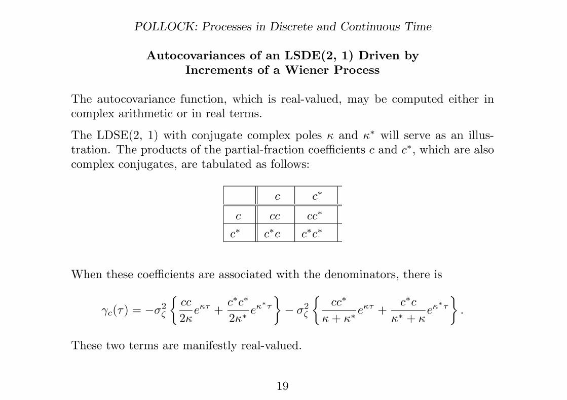
Autocovariances of an LSDE(2, 1) Driven byIncrements of a Wiener Process

The autocovariance function, which is real-valued, may be computed either incomplex arithmetic or in real terms.

The LDSE(2, 1) with conjugate complex poles κ and κ∗ will serve as an illus-tration. The products of the partial-fraction coefficients c and c∗, which are alsocomplex conjugates, are tabulated as follows:

c c∗

c cc cc∗

c∗ c∗c c∗c∗

When these coefficients are associated with the denominators, there is

γc(τ) = −σ2ζ

{cc

2κeκτ +

c∗c∗

2κ∗ eκ∗τ

}− σ2

ζ

{cc∗

κ + κ∗ eκτ +c∗c

κ∗ + κeκ∗τ

}.

These two terms are manifestly real-valued.

19


Autocovariances of an LSDE(2, 1) in Real Terms

We may note that, if κ = δ + iω, κ∗ = δ − iω, and c = α + iβ, c∗ = α − iβ, then

ψ(t) = ceκτ + c∗eκ∗τ

= 2eδτ{α cos(ωτ) − β sin(ωτ)}

Within the expression for the autocovariance function γc(τ), there are

κκ∗ = δ2 + ω2, κ + κ∗ = 2δ cc∗ = α2 + β2,

c2κ∗ = (α + iβ)2(δ − iω) = δ(α2 − β2) + 2αβω + i{2αβδ − ω(α2 + β2)

},

and (c∗)2κ can be obtained from c2κ∗ by replacing i by −i. Therefore,

γc(τ) =σ2

ζ

δ2 + ω2eδτ

{{2αβω − δ(α2 − β2)

}cos(ωτ)

−{2αβδ + ω(α2 − β2)

}sin(ωτ)

}− cos(ωτ)

(α2 + β2)δ

.

20


Estimation of a Frequency-Limited LSDE by Impulse Invariance

The principle of impulse invariance proposes that the discrete-time transfer func-tion should be matched to the continuous-time function by equating the ordinatesof the two impulse response functions at the sample points, such that∑

j

djµτj =

∑j

cjeκjτ for τ ∈ {0, 1, 2, . . .}.

This can be achieved by setting dj = cj and µj = eκj for j = 1, 2, . . . , p..

If all of the poles of the continuous-time model are real-valued, then the mappingfrom the continuous-time poles to the discrete-time poles is invertible, and κj =lnµj for all j. A necessary restriction on the ARMA poles is that µ > 0.

When the poles are complex-valued, the expression µ = eκ represents a many-to-one mapping from a set of continuous-time parameters to a discrete-time pa-rameter. Then, with κ = δ + iω, there is

µ = eκ = eδeiω = eδ{cos(ω + 2πn) + i sin(ω + 2πn)},

where n is an arbitrary integer. Therefore, a restriction is required on the rangeof ω, such as ω ∈ [0, π].

21


Estimation of the Unlimited LSDE by the Autocovariance Principle

In the case where ζ(t) is from a Wiener process, the autocovariance function ofthe LSDE model φ(D)y(t) = θ(D)ζ(t) is

γc(τ) = σ2ζ

∑i

{∑j

cicj−eκiτ

κi + κj

}.

The roots of κ1, . . . , κp of φ(s) are inferred from the roots of α(z) of the ARMAmodel. The parameters of θ(s), can be obtained from the p partial-fractioncoefficients in c = [c1, . . . , cp]′ that equate the continuous time autocovaianceswith the discrete-time values γd(τ) at the sample points.

Let the equations γc(c, τ) = γd(τ); τ = 0, . . . , p − 1 be denoted, in vector form,by γc(c) − γd = 0. Then, the (r + 1)-th Newton–Raphson approximation to thesolution of the equations is

c(r+1) = c(r) + [Dγa(c)]−1(r)[γa(c) − γd](r),

where Dγa(c) is the matrix of the derivatives of γa in respect of c.

Once the definitive value of the vector c is available, we can solve the equations

cj

∏i �=j

(κj − κi) = θ(κj); j = 1, . . . , p

for the coefficients θ0, . . . , θp−1 of θ(s).

22


Frequency-Limited Processes and OverSampling.

In the case of a frequency-limited discrete-time process that is supported on theentire Nyquist interval [−π, π], the corresponding continuous trajectory can becreated by attaching a scaled sinc function or a Dirichlet kernel to each of thediscrete ordinates.

In the case of a finite data sequence, the Dirichlet function interpolation isequivalent to an ordinary Fourier interpolation.

If the sampling is of a rate in excess of the maximum data frequency, then thespectrum of the data, or its periodogram, will exhibit a dead space of zero valuesrunning from the maximum data frequency up to the Nyquist frequency of πradians per sampling interval.

Before fitting an ARMA model to frequency-limited data, it is appropriate toreconstitute the continuous trajectory before sampling it at a lower rate, so as toextend the spectral structure over the entire Nyquist interval.

The consequences of fitting an AR model to frequency-limited data are illustratedin the following slides.

23


00.010.020.030.04

0−0.01−0.02−0.03−0.04−0.05

1970 1975 1980 1985 1990 1995 2000 2005

Figure 6. The deviations of the logarithmic quarterly index of real US GDPfrom an interpolated trend. The observations are from 1968 to 2007. The trendis determined by a Hodrick–Prescott (Leser) filter with a smoothing parameterof 1600.

24


0

0.0002

0.0004

0.0006

0 π/4 π/2 3π/4 π

Figure 7. The periodogram of the data points of Figure 1 overlaid by the para-metric spectral density function of an estimated regular AR(2) model.

25


0

0.0005

0.001

0 π/4 π/2 3π/4 π

Figure 8. The periodogram of the data points of Figure 1 overlaid by the spectraldensity function of an AR(2) model estimated from band-limited data.

26


0

1

2

3

0 π/4 π/2 3π/4 π

Figure 9. The parametric spectrum of the oversampled ARMA(2, 2) process,represented by a heavy line, supported on the spectrum of a white-noise contam-ination, together with the parametric spectrum of an AR(2) model fitted to thesampled autocovariances.

27


0

2.5

5

7.5

10

12.5

0 π/4 π/2 3π/4 π

Figure 10. The parametric spectrum of an ARMA(2, 2) process, limited infrequency to π radians per period and oversampled at the rate of 4 observationsper period, represented by a heavy line, together with the parametric spectrumof an AR(2) model fitted to the sampled autocovariances.

28

POLLOCK: Band-Limited Processes

− i

i

−1 1Re

Im

− i

i

−1 1Re

Im

Figure. The pole-zero diagram of the ARMA(2, 2) model (left) and the diagram showing

location of the poles of the AR(2) model estimated from band-limited data contaminated by

white-noise errors of observation (right).


Explaining the Results

The results of these experiments can be explained by reference to the autocovari-ance function.

In the absense of noise contamination

When the rate of sampling is excessive, the autocovariances will be sampledat points that are too close to the origin, where the variance is to be found.Then, their values will decline at a diminished rate. The reduction in the rateof convergence is reflected in the modulus of the estimated complex roots, whichunderstates the rate of damping.

When there is noise contamination

The variance of the white-noise errors of observation will be added to the vari-ance of the underlying process. Nothing will be added to the adjacent sampledordinates of autocovariance function. Therefore, the sampled autocovarianceswill decline at an enhanced rate.

If this rate of convergence exceeds the critical value, then there will be a tran-sition from cyclical convergence to monotonic convergence, and the estimatedautoregressive roots will be real-valued. This belies the cyclical nature of thetrue process.

30


Resampling the Data

We propose to deal with problems of oversampled data by reducing the rate ofsampling.

The first step is to reconstitute a continuous trajectory from the Fourier ordinatesthat lie within the frequency band in question.

The second step is to sample the continuous trajectory at the rate that is preciselyattuned to the highest frequency that it contains. Then, an ARMA model canbe fitted in the usual way to the resampled data.Two computer programs are available at the address

http://www.le.ac.uk/users/dsgp1/

The program BLIMDOS generates pseudo-random band-limited data (i.e. over-sampled data) from an ARMA model specified by the user. An ordinary ARMAmodel can be fitted to these data and the resulting biases can be assessed.

The program OVERSAMPLE samples the continuous autocovariance function of anARMA model and it proceeds to infer the parameters of an ARMA model ofspecified orders from these sampled ordinates. In this way, it determines theprobability limits of the misspecified estimators.

31


0

0.2

0.4

0.6

0 π/4 π/2 3π/4 π

Figure 11. The periodogram of the data that have been filtered and subsampledat the rate of 1 observation in 4 overlaid by the parametric spectrum of anestimated ARMA(2, 1) model.

32


Characteristics of Band-Limited Processes

A function that is limited in frequency is also an analytic function. Such functionspossess derivatives of all orders. Therefore the turning points of a frequency-limited business cycle trajectory can be located by finding where its derivativesare zero-valued.

A knowledge of a sufficient number of ordinates of an analytic function or ofits derivatives should serve to specify the function completely. Therefore, itseems that band-limited stochastic processes should be perfectly predictable. Theelectrical engineers seem to be convinced of this.

To form a perfect prediction, one would need to have a denumerable infinity ofsampled values, and there should be no errors of observation. The theoreticalpredictability of such a process depends on the infinite supports of the frequen-cybounded sinc functions with the effect that every observation comprises tracesof every sinc function.

The perfect predictability of band-limited processes is an analytic fantasy of thesort that Laplace derided in a famous passage, of which the intention is oftenmisunderstood by chaos theorists and others.

33


Laplacian Determinism

Laplace accepted that the events of the universe must obey the laws of nature.Nevertheless, he proposed that a statistical approach is needed in describingthese events, on account of our inability to comprehend more than a few of theinnumerable factors and circumstances that affect each outcome:

“We may regard the present state of the universe as the effect of its pastand the cause of its future.

An intellect which, at a certain moment, would know all forces thatset nature in motion, and all positions of all items of which nature iscomposed, if it were also vast enough to submit these data to analysis,would embrace, in a single formula, the movements of the greatest bodiesof the universe and those of the tiniest atom.

For such an intellect, nothing would be uncertain and the future, asmuch as the past, would be present before its eyes.”

Pierre-Simon Laplace, (1814), Essai Philosophique sur les Probabilites.

34

processes in discrete and continuous time · wavelets analysis and in digital signal processing,...

Documents