process capability estimation for non--normal quality ... · process capability estimation for...
TRANSCRIPT

ANZIAM J 49 (EMAC2007) ppC642ndashC665 2008 C642
Process capability estimation for nonndashnormalquality characteristics A comparison ofClements Burr and BoxndashCox Methods
S Ahmad1 M Abdollahian2 P Zeephongsekul3
(Received 31 July 2007 revised 27 May 2008)
Abstract
In todayrsquos competitive business environment it is becoming morecrucial than ever to assess precisely process losses due to non-complianceto customer specifications To assess these losses industry is widelyusing process capability indices for performance evaluation of theirprocesses Determination of the performance capability of a stableprocess using the standard process capability indices requires that theunderlying process data should follow a normal distribution How-ever if the data is non-normal measuring process capability usingconventional methods can lead to erroneous results Different processcapability indices such as Clements percentile method and data trans-formation method have been proposed to deal with the non-normal
See httpanziamjaustmsorgauojsindexphpANZIAMJarticleview357for this article ccopy Austral Mathematical Soc 2008 Published June 11 2008 ISSN1446-8735
Contents C643
situation Although these methods are practiced in industry there isinsufficient literature to assess the accuracy of these methods undermild and severe departures from normality This article reviews theperformances of the Clements nonndashnormal percentile method the Burrbased percentile method and BoxndashCox method for non-normal casesA simulation study using Weibull Gamma and Lognormal distribu-tions is conducted Burrrsquos method calculates process capability indicesfor each set of simulated data These results are then compared withthe capability indices obtained using Clements and BoxndashCox methodsFinally a case study based on real world data is presented
Contents
1 Introduction C644
2 Methods to estimate process capability for non-normalprocess C64521 Clements percentile method C64622 BoxndashCox power transformation method C64723 The Burr percentile method C647
3 A simulation study C64931 Comparison criteria C64932 Simulation runs C65333 Discussion C654
4 Case studies C65841 Example 1 C65842 Example 2 C659
5 Conclusions C660
References C662
1 Introduction C644
1 Introduction
Process mean micro process standard deviation σ and product specifications arebasic information used to evaluate process capability indices However prod-uct specifications are different in different products [10] A frontline managerof a process cannot evaluate process performance using micro and σ only Forthis reason Juran [9] combined process parameters with product specifica-tions and introduced the concept of Process capability indices (pci) Sincethen the most common indices being applied by manufacturing industryare process capability index Cp and process ratio for off-center process Cpkdefined as
Cp =Allowable process spread
Actual process=Ut minus Lt
6σ (1)
Cpk = minCpu Cpl (2)
Cpu =Ut minus Lt
3σ Cpl =
microminus Lt3σ
(3)
where Ut and Lt are the upper and lower tolerance limit respectively andCpu and Cpl refer to the upper and lower one sided capability indices In theactual manufacturing process micro and σ are unknown and are often estimatedusing historical data [14] Note that Cp is applied to determine processcapability with bilateral specifications whereas Cpu and Cpl are applied toprocess capability with unilateral specification
The capability indices Cp and Cpk are essentially statistical measures andtheir interpretations rely on the validity of certain assumptions Some of thebasic assumptions of traditional process capability indices are that
bull the process under examination must be under control and stable
bull the output data must be independent and normally distributed
However these assumptions are not usually fulfilled in practice Many phys-ical processes produce non-normal data and quality practitioners need to
2 Methods to estimate process capability for non-normal process C645
verify that the above assumptions hold before deploying any pci techniquesto determine the capability of their processes This article discusses processcapability techniques in cases where the quality characteristics data is non-normal and then compare the accuracy of these pcis using Burr XII distri-bution [1] instead of the Pearson family of curves employed in the Clementspercentile method [4] For illustrative purposes we perform a comparisonstudy of Burr based pci with Clements and BoxndashCox [3] power transforma-tion methods Finally Section 4 presents two application examples with realdata
2 Methods to estimate process capability
for non-normal process
When the distribution of the underlying quality characteristics data is notnormal there have been some modifications of the conventional pcis pre-sented in the quality control literature to resolve the issue of non-normalityKotz and Johnson [7] presented a detailed overview of the various approachesrelated to pcis for non-normal data One of the more straightforward ap-proaches is to transform the non-normal output data to normal data John-son [5] proposed a system of distributions based on the moment methodcalled the Johnson transformation system Box and Cox [3] also used trans-formations for non-normal data by presenting a family of power transforma-tions which includes the square-root transformation proposed by Somervilleand Montgomery [13] to transform a skewed distribution into a normal oneThe main objective of all these transformations is that once the non-normaldata is transformed to normal data one then apply the same conventionalprocess capability indices which are based upon the normal assumptionClements [4] proposed another approach to handle non-normal data thisis called a quantile based approach and provides an easy method to assessthe capability indices for non-normal data Clements used non-normal per-
2 Methods to estimate process capability for non-normal process C646
centiles to modify the classical capability indices
21 Clements percentile method
The Clements Method is popular among quality practitioners in industryClements [4] proposed that 6σ in equation (1) be replaced by the lengths ofinterval between the upper and lower 0135 percentage points of the distri-bution of X that is the denominator in equation (1) is replaced by UpminusLp
Cp =Ut minus LtUp minus Lp
(4)
where Up is the upper 99865 percentile and Lp is the lower 0135 percentileof the observations respectively Since the median M is the preferred centralvalue for a skewed distribution he also defined
Cpu =Ut minusMUp minusM
(5)
Cpl =M minus LtM minus Lp
(6)
and Cpk = minCpu Cpl (7)
The Clements Method uses the standard estimators of skewness and kurtosisthat are based on third and fourth moments respectively which may not bereliable for very small sample sizes [12] These third and fourth momentsare then used to fit a suitable Pearson distribution using the data set Theupper and lower percentiles are then obtained from the selected Pearsondistribution Wu et al [15] conducted research indicating that the ClementsMethod cannot accurately measure the capability indices especially whenthe underlying data distribution is skewed
2 Methods to estimate process capability for non-normal process C647
22 BoxndashCox power transformation method
Box and Cox [3] proposed a family of power transformations on a necessarilypositive response variable X given by
X(λ) =
Xλ minus 1
λ if λ 6= 0
ln(X) if λ = 0 (8)
This transformation depends upon a single parameter λ that is estimatedusing Maximum Likelihood Estimation (mle) [9] The transformation ofnon-normal data to normal data using BoxndashCox transformation is availablein most statistical software packages consequently the users can deploy thistechnique directly to evaluate pcis
23 The Burr percentile method
Burr [1] proposed a distribution called Burr XII distribution to obtain therequired percentiles of a variate X The probability density function of aBurr XII variate Y is
f(y|c k) =
ckycminus1
(1 + yc)k+1 if y ge 0 c ge 1 k ge 1
0 if y lt 0
(9)
where c and k represent the skewness and kurtosis coefficients of the Burrdistribution respectively
Liu and Chen [12] introduced a modification based on the Clementsmethod whereby instead of using Pearson curve percentiles they replacedthem with percentiles from an appropriate Burr distribution The proposedmethod is outlined in the following steps and also illustrated by an examplewith Ut = 32 and Lt = 4 in Table 1
2 Methods to estimate process capability for non-normal process C648
1 Estimate the sample mean x sample standard deviation s skewness s3
and kurtosis s4 of the original sample data Note that
s3 =n
(nminus 1)(nminus 2)
sum (xj minus xs
)3
and s4 =n(n+ 1)
(nminus 1)(nminus 2)(nminus 3)
sum (xj minus xs
)4
minus 3(nminus 1)2
(nminus 2)(nminus 3)
2 Calculate standardized moments of skewness α3 and kurtosis α4 as
α3 =(nminus 2)radicn(nminus 1)
s3 (10)
and α4 =(nminus 2)(nminus 3)
(n2 minus 1)s4 + 3
(nminus 1)
(n+ 1) (11)
The kurtosis defined by (11) is commonly known as the excess kurtosissince it adjusts the ordinary kurtosis value above and below the value of+300 (which indicates the absence of kurtosis that is the distributionis mesokurtic) Negative value identifies a platykurtic distribution andpositive value that of a leptokurtic distribution
3 Use the values of α3 and α4 to select the appropriate Burr parametersc and k [1] Then use the Burr distribution XII [2] to obtain thedistribution of the standardized variate
Z =Y minus microσ
where Y is the selected Burr variate micro and σ its corresponding meanand standard deviation respectively The means and standard devia-tions as well as skewness and kurtosis coefficients for a large collectionof Burr distributions are found in tables of Burr [2] Liu and Chen [12]From these tables the standardized 000135 05 099865 percentiles
3 A simulation study C649
that is Z000135 Z05 and Z099865 are obtained Obtain correspondingpercentiles of X by matching the two standardized values that is
X minus xs
=Y minus microσ
(12)
4 From (12) the estimated percentiles for lower median and upper per-centiles are
Lp = x+ sZ000135 (13)
M = x+ sZ05 (14)
and Up = x+ sZ099865 (15)
5 Calculate process capability indices using equations (4) to (7)
Instead of using moments of skewness and kurtosis as we have done hereother methods such as Maximum Likelihood Method of Probability-WeightedMoments and Method of L-Moments [11] are also used to estimate parame-ters of a Burr distribution However our choice is determined by the fact thatquality control practitioners with little background in theoretical statisticswill find the estimation procedure adopted here which is simply a momentmatching process much easier to comprehend and apply
3 A simulation study
31 Comparison criteria
Different comparison yardsticks lead to different conclusions A widely rec-ognized yardstick for tackling the non-normality problem for pci estimationis given by Rivera et al [8] They used upper tolerance limits of the under-lying distributions to calculate the actual number of non-conformance items
3 A simulation study C650
Table 1 PCI calculations using Burr Percentile MethodProcedure Parameters Calculated valuesEnter specificationsUpper tolerance limit Ut 32Lower tolerance limit Lt 4Estimate sample statisticsSample size n 100Mean x 105Standard deviation s 3142Skewness s3 114Kurtosis s4 258Use s3 and s4 to calculateStandardized moment of skewness α3 112Standardized moment of kurtosis α4 497Based on α3 and α4 select c and k
c 2347k 4429
Use the estimated Burr XII distribution to obtainstandardized lower percentile Z000135 minus1808standardized median Z05 minus0140standardized upper percentile Z099865 4528Calculate estimated 0135 percentile using (14) Lp 4819Calculate estimated median using (15) M 1006Calculate estimated 99865 percentile using (15) Up 24727Calculate CPIs using (4)ndash(7) Cp 140
Cpu 149Cpl 115Cpk 115
3 A simulation study C651
and equivalent Cpk values Estimated Cpk values calculated from the dataare then compared with the target Cpk values A similar motivated schemehas been used as a comparison yardstick for one-sided Cpu by Tang et al [9]and Liu and Chen [12] in their non-normal pcis studies For a target Cpuvalue the fraction of non-confirming items from a normal distribution canbe determined using
Fraction of non-conforming parts = Φ(minus3Cpu) (16)
where Φ(x) refers to the cumulative distribution function of the standardnormal random variable [6]
In this article the process capability index Cpu with unilateral tolerancelimit is used as comparison criterion Weibull Gamma and Lognormal distri-butions are used to investigate the effect of non-normal data on the processcapability index These distributions are known to have parameter valuesthat represent mild to severe departures from normality These parametersare selected to compare our simulation results with existing results using thesame parameters as Tang amp Than [9] and Liu amp Chen [12]
The probability density functions of Weibull Gamma and Lognormaldistributions are
Weibull(α β) α gt 0 β gt 0
f(x|α β) =α
βxαminus1eminusx
αβ x ge 0
Gamma(α β) α gt 0 β gt 0
f(x|α β) =1
γ(α)βαxαminus1eminusxβ x ge 0
Lognormal(micro σ2) minusinfin lt micro ltinfin
f(x|micro σ2) =1radic
2πσ2xeminus(lnxminusmicro)22σ2
x ge 0
In our simulation study for comparison purposes the target Cpu values of 0510 15 and 20 and the Weibull distribution with α = 12 and β = 10
3 A simulation study C652
Gamma distribution with α = 10 and β = 10 and Lognormal distributionwith micro = 0 and σ2 = 10 are used The corresponding Ut value for eachdistribution is
Ut = Cpu(X099865 minusX05) +X05 (17)
where X099865 and X05 are the designated percentiles of the correspondingdistribution For example if Cpu = 15 and the underlying distribution is sayWeibull with parameter values α = 12 and β = 1 then using any statisticalpackage one obtain the two percentiles which areX099865 = 48236 andX05 =07368 respectively Then we use equation (17) to find the corresponding Utwhich equals 6867
We next simulate 30 samples each of size 100 from each distribution andfollow the steps outlined below to calculate the corresponding Cpu for eachsample
1 Choose a distribution with known parameters for example Weibullα = 12 and β = 1
2 Find X099865 and X05 for this distribution using any statistical package
3 Choose a target Cpu value say Cpu = 15
4 Use (17) to calculate Ut which equals 6867 for this example
5 Next we compare between the three methods Clements Box-Cox andBurr using the next series of steps
6 Simulate values from underlying distribution
7 Use each method to estimate X099865 and X05
8 For a target Cpu value say 15 and corresponding Ut value say 6867calculate the Cpu values using all three methods (similar to Table 1)
3 A simulation study C653
9 Compare these calculated Cpu values using standard statistical mea-sures and graphs to decide which among the three methods leads tothe most accurate estimate of the target Cpu value
The main criteria used to compare between the three methods is to determinethe precision and accuracy of process capability estimations The best andmost suitable method will have the mean of the estimated Cpu values closestto the target value (that is greatest accuracy) and will have the smallestvariability measured by standard deviation of the estimated values [9] (thatis greatest precision)
32 Simulation runs
As discussed in Section 31 we generate 30 samples each of size 100 fromspecific Weibull Gamma and Lognormal distributions After each simula-tion run the necessary statistics such as mean standard deviation medianskewness kurtosis upper and lower 0135 percentiles were obtained In thisarticle Cpu is used as comparison criterion The capability index for thenon-normal data should be compatible with that computed under normalityassumption given the same fraction of non-conforming parts [9] The esti-mates for Cpu were determined using Burr Clements and BoxndashCox methodssteps outlined in Section 31 The average value of all 30 estimated valuesand their standard deviations were calculated and presented in Tables 2ndash4
To investigate the most suitable method for dealing with non-normalitypresented by Weibull Gamma and Lognormal distributions we present boxplots of estimated Cpu values using all three methods (Figures 1ndash3) Box plotsare able to graphically display important features of the simulated Cpu valuessuch as median inter-quartile range and existence of outliers These figuresindicate that the means using Burr method is closest to their targeted Cpuvalues and the spread of the values is smaller than that using Clements
3 A simulation study C654
Table 2 The mean and standard deviation of 30Cpu values with n = 100(Weibull)
Burr Clements Box-CoxCpu Ut mean Std mean Std mean Std05 2780 0596 0090 0590 0099 0621 010010 4824 1152 0159 1159 0175 0956 019415 6867 1708 0228 1727 0252 1204 028320 8910 2264 0297 2296 0328 1407 0367
Table 3 The mean and standard deviation of 30Cpu values with n = 100(Gamma)
Burr Clements Box-CoxCpu Ut mean Std mean Std mean Std05 3650 0578 0091 0593 0105 0611 007510 6608 1117 0166 1159 0188 0897 013215 9565 1655 0241 1725 0271 1099 018520 12522 2194 0316 2290 0354 1262 0233
method therefore indicating a better approximation BoxndashCox method givescomparable results for smaller target values
33 Discussion
As mentioned in Section 31 the performance yardstick is to determine theaccuracy and precision for a given sample size To determine accuracy welooked at the mean of the estimated Cpu values and for precision we focusedon the standard deviation of these values using all three methods Looking
3 A simulation study C655
Table 4 The mean and standard deviation of 30Cpu values with n = 100(Lognormal)
Burr Clements Box-CoxCpu Ut mean Std mean Std mean Std05 4482 0499 0084 0496 0097 0503 004810 8339 1024 0166 1031 0183 0710 006115 12009 1523 0243 1541 0265 0832 007020 15679 2022 0320 2050 0348 0921 0076
Figure 1 Box plot of estimated Cpu values with target Cpu = 05 10 15and 20 for Weibull distribution
3 A simulation study C656
Figure 2 Box plot of estimated Cpu values with target Cpu = 05 10 15and 20 for Gamma distribution
3 A simulation study C657
Figure 3 Box plot of estimated Cpu with target Cpu = 05 10 15 and 20for Lognormal distribution
4 Case studies C658
at the results depicted in Tables 2ndash4 we conclude that
1 The Burr method is the one for which the mean of the estimated valuedeviates least from the targeted Cpu values
2 The standard deviation of the estimated Cpu values using the Burrmethod is smaller than Clements method
3 BoxndashCox method does not yield results close to any targeted Cpu valuesexcept for smaller targeted values
During our simulation exercises we also observed that larger sample sizesyield better estimates for all methods Therefore sample size does havean impact on process capability estimate It was also observed that largertargeted Cpu values led to slightly worse estimates for all methods
4 Case studies
41 Example 1
The real data set consisting of 30 independent samples each of size 50 isfrom a semiconductor manufacturing industry The data are measurementsof bonding area between two surfaces with upper specification Ut = 2413 Initially an X-R chart was used to check whether or not the process isstable before further analysis of the experimental data Figure 4 shows thehistogram of the data Using a Goodness of Fit Test the data is best fittedby a Gamma distribution with α = 25438 and β = 000921
We used all three methods to estimate Cpu The mean and standarddeviation of the estimated Cpu values using each method is presented inTable 5 The actual Cpu value of this process derived using equation (5)
4 Case studies C659
Figure 4 Histogram of data from a semiconductor industry
and based on 1500 products is 03775 The results in Table 5 show that themean value obtained using Burr method is closest to the actual value
42 Example 2
In the second case study we present a capability analysis using a real setof data obtained from a computer manufacturing industry in Taiwan [15]Again the analysis is based on 30 independent samples each of size 50 Thedata set has the one sided specification limit Ut = 02 mm Figure 5 showsthe histogram of the data which shows that the underlying distribution is notnormal and is right skewed However the data do not appear to be best fitted
5 Conclusions C660
Table 5 Process capability analysis results for semiconductor data
Method Ut Cpu mean Cpu StdClements 2413 04368 00934Burr 2413 04207 00768BoxndashCox 2413 04999 00608
Table 6 Process capability analysis results for computer manufacturingprocess
Method Ut Cpu mean Cpu StdClements 02 mm 20432 04354
Burr 02 mm 19251 03490Box-Cox 02 mm 12431 02266
by any of the distributions we have used in this paper All three methodshave been applied to estimate process capability of this right skewed dataThe estimated Cpu results are displayed in Table 6 The actual Cpu value ofthis process is 18954 and one of the reasons for selecting this example is tocompare the three methods for a process where the capability index is greaterthan 15 The results in Table 6 again show that mean value obtained usingthe Burr method is closest to the actual value
5 Conclusions
The main purpose of this article is to compare and contrast between threemethods of obtaining process capability indices and determine which methodis more capable in achieving higher accuracy in estimating these indices for
5 Conclusions C661
Figure 5 Histogram of measurement data from a computer manufacturingprocess
References C662
non-normal quality characteristics data Simulation study indicates thatBurrrsquos method generally provides better estimate of the process capabilityfor non-normal data Finally two real examples from industry are presentedThe results using these experimental data show that the estimated Cpu valuesobtained using Burr method are closest to the true values compare to othermethods In conclusion Burr method is therefore deem to be superior tothe other two methods for estimating the process capability indices for non-normal data However we strongly recommend further investigation of theBurr method for calculating pcis for data whose underlying distributionsshow significant departures from normality
Acknowledgements We thank the anonymous referees and the Editorwhose suggestions helped to improve the original version of this paper
References
[1] I W Burr (1942) Cumulative frequency distribution Ann Math Stat13 215ndash232 httpwwwamsorgmathscinetpdf6644pdf C645C647 C648
[2] I W Burr (1973) Parameters for a general system of distributions tomatch a grid of α3 and α4 Commun Stat 21ndash21httpwwwzentralblatt-mathorgzmathsearchq=an
03413665amptype=pdfampformat=complete C648
[3] G E P Box and D R Cox (1964) An analysis of transformationJ Roy Stat Soc B 26211ndash252httpwwwjstororgview00359246di99315299p024930
C645 C647
[4] J A Clements (1989) Process capability calculations for non-normaldistributions Quality Progress 2295ndash100
References C663
httpwwwasqorgqicdisplay-itemindexhtmlitem=14059
C645 C646
[5] N L Johnson (1949) System of frequency curves generated bymethods of translation Biometrika 36149ndash176httpwwwjstororgview00063444di99230099p0220l0 C645
[6] S Kotz and C R Lovelace (1998) Process capability indices in theoryand practice Arnold London httpwwwamazoncomProcess-Capability-Indices-Theory-Practicedp0340691778
C651
[7] S Kotz and N L Johnson (1993) Process capability indices NewYork Chapman amp Hall httpwwwamazoncomProcess-Capability-Indices-Samuel-Kotzdp041254380X C645
[8] L A R Rivera N F Hubele and F D Lawrence (1995) Cpk indexestimation using data transformation Comput Ind Engng 29 55-58httpwwwingentaconnectcomcontentels036083521995
0000002900000001art00045 C649
[9] L C Tang S E Than (1999) Computing process capability indicesfor non-normal data a review and comparative study Qual ReliabEngng Int 15 339ndash353 doiCCC 0748-801799050339 C644 C647C651 C653
[10] D Montgomery (1996) Introduction to Statistical Quality Control 5thedition Wiley New York httpbcswileycomhe-bcsBooksaction=indexampbcsId=2077ampitemId=0471656313 C644
[11] J OrsquoConnell and Q Shao (2004) Further investigation on a newapproach in analyzing extreme events CSIRO Mathematical andInformation Sciences Report No 0441httpwwwcmiscsiroautechreportsdocsx0000ihwpdf C649
References C664
[12] PeindashHsi Liu and FeindashLong Chen (2006) Process capability analysis ofnon-normal process data using the Burr XII distribution Int J AdvManuf Technol 27 975ndash984 doi101007s 00170-004-2263-8 C646C647 C648 C651
[13] S Somerville and D Montgomery (1996) Process capability indicesand non-normal distributions Quality Engineering 19(2)305ndash316doi10108008982119608919047 C645
[14] F K Wang (2006) Quality evaluation of a manufactured product withmultiple characteristics Qual Relib Engng Int 22 225ndash236httpdoiwileycom101002qre712 C644
[15] H H Wu J S Wang and T L Liu (1998) Discussions of theClements-based process capability indices In Proceedings of the 1998CIIE National Conference pp561ndash566 doi101007s 00170-004-2263-8C646 C659
References C665
Author addresses
1 S Ahmad School of Mathematical and Geospatial Sciences RMITUniversity Melbourne Victoria Australia
2 M Abdollahian School of Mathematical and Geospatial SciencesRMIT University Melbourne Victoria Australia
3 P Zeephongsekul School of Mathematical and Geospatial Sciencesand School of Mathematical and Geospatial Sciences RMITUniversity Melbourne Victoria Australia
- Introduction
- Methods to estimate process capability for non-normal process
-
- Clements percentile method
- Box--Cox power transformation method
- The Burr percentile method
-
- A simulation study
-
- Comparison criteria
- Simulation runs
- Discussion
-
- Case studies
-
- Example 1
- Example 2
-
- Conclusions
- References
-
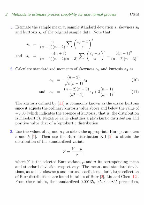
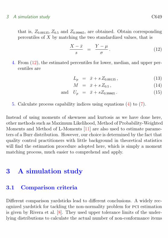
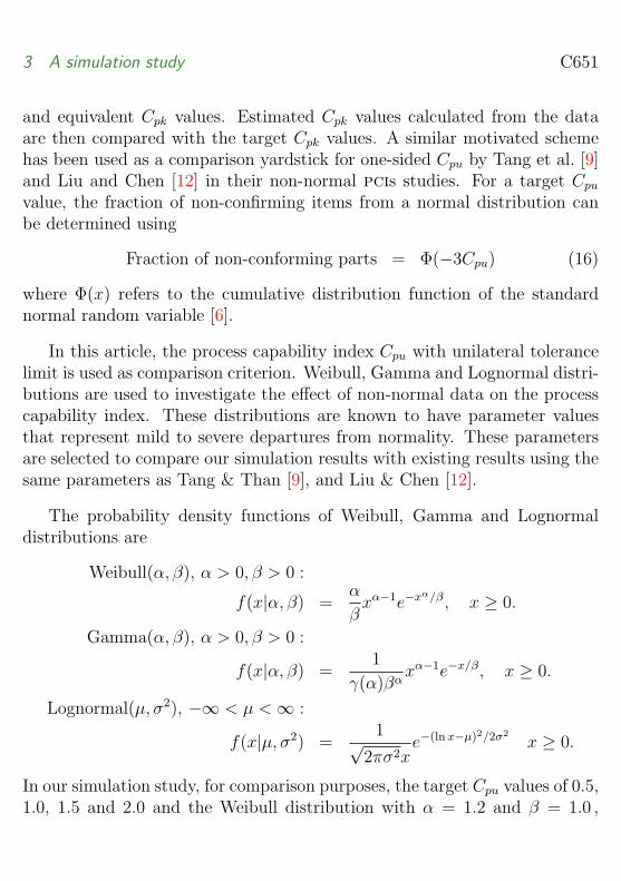
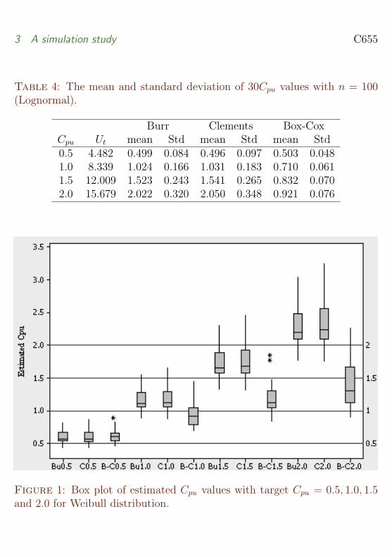
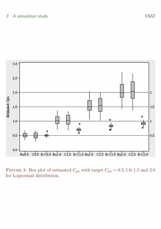
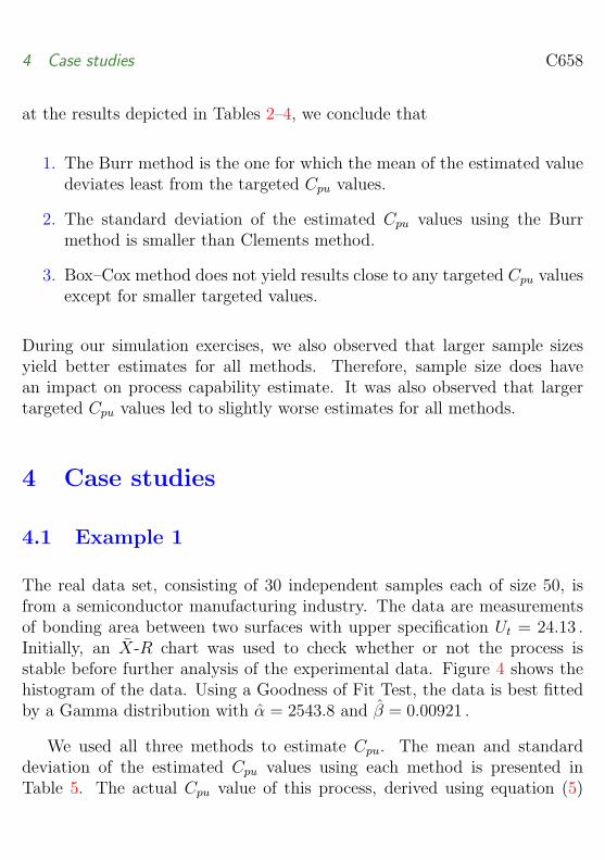
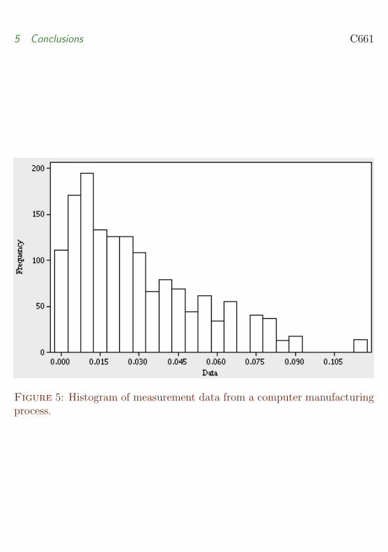