proceedings oft the cp-03 workshop on€¦ · · 2009-04-07proceedings of the cp 2004 workshop on...

Proceedings of the CP 2004 Workshop on CSP Techniques with Immediate Application

(CSPIA)

Roman Barták Ulrich Junker

Marius-Calin Silaghi Markus Zanker

(editors)

Held at the

International Conference on Principles and Practice of Constraint Programming

CP-2004 September 27th, 2004

Toronto, Canada

ORGANISATION

Organizers and Workshop Chairs Roman Barták, Charles University, [email protected]

Ulrich Junker, ILOG, [email protected]

Marius-Calin Silaghi, Florida Institute of Technology, [email protected]

Markus Zanker, University Klagenfurt, [email protected]

Program Committee Roman Barták, Charles University, [email protected]

Frederic Benhamou, University of Nantes, [email protected]

Berthe Choueiry, University Nebraska Lincoln, [email protected]

Joerg Denzinger, University Calgary, [email protected]

Boi Faltings, EPFL, [email protected]

Alexander Felfernig, University Klagenfurt, [email protected]

Christian Frei, ABB Switzerland, [email protected]

Gerhard Friedrich, University Klagenfurt, [email protected]

Dietmar Jannach, University Klagenfurt, [email protected]

Pedro Meseguer, Institut d'Investigació en Intelligència Artificial (IIIA), [email protected]

Debasis Mitra, Florida Institute of Technology, [email protected]

Christian Russ, ConfigWorks Informationssysteme & Consulting, Austria, [email protected]

Markus Stumptner, University of South Australia, [email protected]

Barry O'Sullivan, University College Cork, [email protected]

Marc Wallace, Monash University, [email protected]

Franz Wotawa, Technical University Graz, [email protected]

ii

PREFACE Constraint satisfaction is a successful paradigm developed by the AI community that found acceptance in many fields of computer science. While specific techniques (e.g. operations research ones) exist for most of the problems that can be represented as Constraint Satisfaction Problems (CSPs), constraint satisfaction owes its success to the simplicity and straightforwardness with which humans can formalize new problems and profit thereby of powerful existing techniques. While there exist extensive literature about abstract techniques for solving more or less general CSP formulations, the applicability of the field is covered by a veil of mystery. The companies that propose CSP based solutions seem to have particular success on the market but the details and the contribution of the Constraint Satisfaction research to all of it are all but well known. The lack of feedback to the large amount of academic researchers involved in the field encourages a more in breadth research versus a focused research. Moreover, most conferences in the field give currently only little attention to the relation technique/application and focus solely on randomly generated or on toy evaluation criteria. Most problems faced by the researchers trying to apply constraint satisfaction to real applications are invisible to the community as they do not find easily an avenue into the main conferences like CP. The series of applied science - workshops was started at CP 2003 and intends to foster a better interaction between physical reality and academic research on CSPs and to direct CSP research towards areas of high promise and social interest. (All the difference is BFS vs. A*!) This goal of interaction between industry and academia resembles also in the choice of the invited speaker: Mark Wallace addresses the issue when industry meets research and discusses three successful application areas in transport industry. The working notes of this workshop gather contributions from applications such as interactive configuration, computer graphics, order sequencing and model checking of UML diagrams. Furthermore, research on search techniques and DisCSPs with a focus on its applicability is presented. The 8 papers demonstrate that continuous technical advances in CSPs lead to a technology that fits more and more real applications.

Roman Barták Ulrich Junker

Marius-Calin Silaghi Markus Zanker

Aug. 25, 2003

iii

CONTENTS Invited talk: Three Research Collaborations with the Transport Industry Mark Wallace 1 Finite Satisfiability of UML class diagrams by constraint programming Marco Cadoli, Diego Calvanese, Giuseppe De Giacomo, Toni Mancini 2-16 Interval Constraints for Computer Graphics Belaid Moa 17-36 Multiplex Dispensation Order Generation for Pyrosequencing Mats Carlsson and Nicolas Beldiceanu 37-51 Boosting Constraint Satisfaction using Decision Trees Barry O'Sullivan, Alex Ferguson, Eugene C. Freuder 52-65 An empirical Study of Heuristic and Randomized Search Techniques in a Real-World Setting Venkata Praveen Guddeti, Hui Zou, Berthe Y. Choueiry 66-82 Desk-mates (Stable Matching) with Privacy of Preferences and a new Distributed CSP Framework Marius-Calin Silaghi, Markus Zanker, Roman Barták 83-96 Comparing two implementations of a Complete and Backtrack-free Interactive Configurator Sathiamoorthy Subbarayan, Rune M. Jensen, Tarik Hadzic, Henrik R. Andersen, Henrik Hulgaard, Jesper Moller 97-111 BBD-based Recursive and Conditional Modular Interactive Product Configuration Erik R. van der Meer, Henrik Reif Andersen 112-126

v

Three Research Collaborations with the Transport Industry

Mark Wallace

Faculty of Information Technology Monash University

Building 63, Clayton Vic 3800 Australia

[email protected]

Abstract. The talk will explore the three problem definitions, and give their business motivation. The projects were about

logistics with depots,

patrol dispatcher and

flight schedule retimer.

The talk will then discuss the algorithms used to solve them, and hopefully also give an insight into the benefits of applications-driven research.

1

Finite Satisfiability of UML class diagrams by

Constraint Programming

Marco Cadoli1, Diego Calvanese2, Giuseppe De Giacomo1, Toni Mancini1

1 Dipartimento di Informatica e SistemisticaUniversita di Roma “La Sapienza”

Via Salaria 113, I-00198 Roma, Italycadoli|degiacomo|[email protected]

www.dis.uniroma1.it/~cadoli|~degiacomo|~tmancini2 Faculty of Computer Science

Free University of Bolzano/BozenPiazza Domenicani 3, I-39100 Bolzano, Italy

[email protected]

Abstract. Finite model reasoning in UML class diagrams, e.g., check-ing whether a class is forced to have either zero or infinitely many objects,is of crucial importance for assessing quality of the analysis phase in soft-ware development. Despite the fact that finite model reasoning is oftenconsidered more important than unrestricted reasoning, no implementa-tion of the former task has been attempted so far. The main result of thispaper is that it is possible to use off-the-shelf tools for constraint model-ing and programming for obtaining a finite model reasoner. In particular,exploiting appropriate reasoning techniques, we propose an encoding asa CSP of UML class diagram satisfiability. Moreover, we show also howCP can be used to actually return a finite model of a class diagram. Adescription of our system, which accepts as input class diagrams in theMOF syntax, and the results of the experimentation performed on theCIM knowledge base are given.

1 Introduction

The Unified Modelling Language (UML, [13], cf. www.uml.org) is probably themost used modelling language in the context of software development, and hasbeen proven to be very effective for the analysis and design phases of the softwarelife cycle.

UML offers a number of diagrams for representing various aspects of therequirements for a software application. Probably the most important diagram isthe class diagram, which represents all main structural aspects of an application.A typical class diagram shows:

– classes, i.e., homogeneous collections of objects, i.e., instances;– associations, i.e., relations between classes;– ISA hierarchies between classes, i.e., relations establishing that each object

of a class is also an object of another class;

2

1..1Curriculum

20..∗

enrolledStudent

Fig. 1. A UML class diagram.

1..1Curriculum

1..1 1..1

20..∗

enrolledStudent

likes

Fig. 2. A UML class diagram with finitely inconsistent classes.

– multiplicity constraints on associations, i.e., restrictions on the number oflinks between objects related by an association.

Actually, a UML class diagram represents also other aspects, e.g., the attributesand the operations of a class, the attributes of an association, and the special-ization of an association. Such aspects, for the sake of simplicity, will not beconsidered in this paper.

An example of a class diagram is shown in Figure 1, which refers to anapplication concerning management of administrative data of a university, andexhibits two classes (Student and Curriculum) and an association (enrolled)between them. The multiplicity constraints state that:

– Each student must be enrolled in at least one and at most one curriculum;– Each curriculum must have at least twenty enrolled students, and there is

no maximum on the number of enrolled students per curriculum.

It is interesting to note that a class diagram induces restrictions on the numberof objects. As an example, referring to the situation of Figure 1, it is possibleto have zero, twenty, or more students, but it is impossible to have any numberof students between one and nineteen. The reason is that if we had, e.g., fivestudents, then we would need at least one curriculum, which in turn requires atleast twenty students.

In some cases the number of objects of a class is forced to be zero. As anexample, if we add to the class diagram of Figure 1 a further likes association,with the constraints that each student likes exactly one curriculum, and thateach curriculum is liked by exactly one student (cf. Figure 2), then it is impos-sible to have any finite non-zero number of students and curricula. In fact, thenew association and its multiplicity constraints force the students to be the ex-actly as many as the curricula, which is impossible. Observe that, with a logicalformalization the UML class diagram, one can actually perform such form ofreasoning making use of automated reasoning tools1.

1 Actually, current CASE tools do not perform any kind of automated reasoning onUML class diagrams yet.

3

1..1

Curriculum

TeachingAssist

1..∗

0..6

20..∗ 1..1

0..3

Student

assigned

enrolled

works

Fig. 3. Another finitely inconsistent class diagram.

Referring to Figure 2, note that the multiplicity constraints do not rule outthe possibility of having infinitely many students and curricula. When a class isforced to have either zero or infinitely many instances, it is said to be finitely

inconsistent or finitely unsatisfiable. For the sake of completeness, we mentionthat in some situations involving ISA hierarchies (not shown for brevity), classesmay be forced to have zero objects, and are thus said to be inconsistent orunsatisfiable in the unrestricted sense.

Unsatisfiability, either finite or unrestricted, of a class is a symptom of abug in the analysis phase, since such a class is clearly superfluous. In particular,finite unsatisfiability is especially relevant in the context of applications, e.g.,databases, in which the number of instances is intrinsically finite.

Obviously the situation described by Figure 2 (in particular, the fact that acurriculum is liked by exactly one student) is not realistic. Anyway, finite incon-sistency may arise in more complex situations, cf. e.g. Figure 3. Here, for budgetreasons, each curriculum has at most six teaching assistants, and, for enforcingeffectiveness of service, each TA is assigned to at most three students. The rea-son why there must be zero (or infinitely many) students is that eighteen, i.e.,three times six, is less than twenty. Global reasoning on the whole class diagramis needed to show finite inconsistency. For large, industrial class diagrams, suchreasoning is clearly not doable by hand.

If, in our application we have that the UML class diagram will always beinstantiated by a finite number of objects (as often is the case), then, for assess-ing quality of the analysis phase in software development, we must take fullyinto account such an assumption. This is reflected in focusing on finite modelreasoning.

In this paper we address the implementation of finite model reasoning onUML class diagrams, a task that has not been attempted so far. This is done byexploiting an encoding of UML class diagrams in terms of Description Logics(DLs) [6, 4].

DLs [1] are logics for representing and reasoning on domains of interest interms of classes and relationships among classes. They are extensively used toformalize conceptual models and object-oriented models in databases and soft-ware engineering, and lay the foundations for ontology languages used in theSemantic Web. From a technical point of view, DLs can be seen as multi-modal

4

logics [16] specifically tailored to capture the typical constructs of class-basedformalisms. Alternatively, they can be seen as well-behaved fragments of first-order logic. Indeed, reasoning in such logics has been studied extensively, bothfrom a theoretical point of view, establishing EXPTIME-completeness of variousDL variants [9], and from a practical point of view, developing practical reason-ing systems. State-of-the-art DL reasoning systems, such as Fact2 and Racer3,are highly optimized and result among the best reasoners for modal logics.

The correspondence between UML class diagrams and DLs allows one touse the current state-of-the-art DL reasoning systems to reason on UML classdiagrams. However, the kind of reasoning that such systems support is unre-stricted (as in first-order logic), and not finite model reasoning. That is, the factthat models (i.e., instantiations of the UML class diagram) must be finite is nottaken into account.

Interestingly, in DLs, finite model reasoning has been studied from a the-oretical perspective, and its computational complexity has been characterizedfor various cases [14, 10, 7, 15]. However, no implementations of such techniqueshave been attempted till now. In this paper we reconsider such work, and on thebasis of it we present, to the best of our knowledge, the first implementation offinite model reasoning in UML class diagrams.

The main result of this paper is that it is possible to use off-the-shelf tools forconstraint modelling and programming for obtaining a finite model reasoner. Inparticular, exploiting the finite model reasoning technique for DLs presentedin [10, 7], we propose an encoding of UML class diagram satisfiability as aConstraint Satisfaction Problem (CSP). Moreover, we show also how constraintprogramming can be used to actually return a finite model of the UML classdiagram.

We built a system that accepts as input a class diagram written in the MOFsyntax, and translates it into a file suitable for ILOG’s oplstudio, which checkssatisfiability and returns a finite model, if there is one. The system allowed us totest the technique on the industrial knowledge base CIM, obtaining encouragingresults.

The rest of the paper is organized as follows: in Section 2 we briefly de-scribe the main constructs of UML class diagrams in terms of first-order logic.In Sections 3 and 4 we then show how to encode the UML class diagram finitesatisfiability problem as a CSP, and, in Section 5 we show how to find, if possi-ble, a finite model of a class diagram, with non-empty classes and associations.Section 6 is devoted to some observations on complexity issues, while our systemis described in Section 7. Finally, Section 8 concludes the paper.

2 Formalization of UML Class Diagrams

UML class diagrams allow for modelling, in a declarative way, the static struc-ture of an application domain, in terms of concepts and relations between them.

2 http://www.cs.man.ac.uk/~horrocks/FaCT/3 http://www.sts.tu-harburg.de/~r.f.moeller/racer/

5

m1..n1

C1

AC2

m2..n2

Fig. 4. Binary association in UML with multiplicity constraints.

C1

A

· · ·

C2

Cn

Fig. 5. n-ary association in UML.

We briefly describe UML class diagrams, and specify the semantics of the mainconstructs in terms of first-order logic (FOL).

A class in a UML class diagram denotes a set of objects with commonfeatures. Names of classes are unique in a UML class diagram. Formally, a classC corresponds to a FOL unary predicate C. Classes may have attributes andoperations, but for simplicity we do not describe them here, since they have onlyminor impact on the reasoning process.

An association in UML is a relation between the instances of two or moreclasses. Names of associations are unique in a UML class diagram. A binary as-sociation A between two classes C1 and C2 is graphically rendered as in Figure 4.The multiplicity m1..n1 on the binary association specifies that each instance ofthe class C1 can participate at least m1 times and at most n1 times to A, simi-larly for C2. When the multiplicity is omitted, it is intended to be 0..∗. Observethat an association can also relate several classes C1, C2, . . . , Cn, as depicted inFigure 54.

An association A between the instances of classes C1, . . . , Cn, can be formal-ized as an n-ary predicate A that satisfies the following FOL assertion:

∀x1, . . . , xn. A(x1, . . . , xn) → C1(x1) ∧ . . . ∧ Cn(xn)

For binary associations (see Figure 4), multiplicities are formalized by the FOLassertions:

∀x. C1(x) → (m1 ≤ ♯{y | A(x, y)} ≤ n1)∀y. C2(y) → (m2 ≤ ♯{x | A(x, y)} ≤ n2)

where we have abbreviated FOL formulas expressing cardinality restrictions.Aggregations, which are a particular kind of binary associations are modeled

similarly.

4 In UML, differently from other conceptual modelling formalisms, such as Entity-Relationship diagrams [2], multiplicities are look-across cardinality constraints [17].This makes their use in non-binary associations difficult with respect to both mod-elling and reasoning.

6

C1 C2 . . . Cn

C

Fig. 6. A class hierarchy in UML.

In UML one can use a generalization between a parent class and a child classto specify that each instance of the child class is also an instance of the parentclass. Hence, the instances of the child class inherit the properties of the parentclass, but typically they satisfy additional properties that in general do not holdfor the parent class. Several generalizations can be grouped together to form aclass hierarchy (also called ISA hierarchy), as shown in Figure 6. Disjointness

and completeness constraints can also be enforced on a class hierarchy (graph-ically, by adding suitable labels). A class hierarchy is said to be disjoint if noinstance can belong to more than one derived class, and complete if any instanceof the base class belongs also to some of the derived classes.

A UML class C generalizing a class C1 can be formally captured by meansof the FOL assertion:

∀x. C1(x) → C(x)

A class hierarchy as the one in Figure 6 is formally captured by means of theFOL assertions:

∀x. Ci(x) → C(x), for i = 1, . . . , n

Disjointness among C1, . . . , Cn is expressed by the FOL assertions

∀x. Ci(x) →∧n

j=i+1¬Cj(x), for i = 1, . . . , n − 1

The completeness constraint expressing that each instance of C is an instanceof at least one of C1, . . . , Cn is expressed by:

∀x. C(x) →∨n

i=1Ci(x)

In UML class diagrams, it is typically assumed that all classes not in the samehierarchy are a priori disjoint. Similarly, it is typically assumed that objects ina hierarchy must belong to a single most specific class. Hence, two classes in ahierarchy may have common instances only if they have a common subclass.

3 Finite Model Reasoning on UML Class Diagrams

As mentioned before, a technique for finite model reasoning in UML class dia-grams can be derived from techniques developed in the context of DescriptionLogics (DLs) [1]. Such techniques are based on translating a DL knowledge base

7

into a set of linear inequalities [10, 7]. The first-order formalization of UML classdiagrams shown in the previous section can be rephrased in terms of DLs. Hence,the finite model reasoning techniques for DLs can be used also for UML classdiagrams.

Intuitively, consider a simple UML class diagram D with only binary as-sociations, and in which we do not make use of generalization and hierarchies.Further, for each association, between two classes multiplicities are specified.Figure 4 shows a fragment of such a diagram, in which we have two classes C1

and C2 and an association A between them. The multiplicities in the figure ex-press that each instance of C1 is associated with at least m1 and at most n1

instances of C2 through the association A, similarly for C2. It is easy to see thatsuch a class diagram D is always satisfiable (assuming mi ≤ ni) if we admitinfinite models. Hence, only finite model reasoning is of interest. We observethat, if D is finitely satisfiable, then it admits a finite model in which all classesare pairwise disjoint. Exploiting this property, we can encode finite satisfiabilityof D in a constraint system as follows. We introduce one variable for each classand one for each association, representing the number of instances of the class(resp., association) in a possible model of D. Then, for each association A weintroduce the constraints:

m1 ∗ c1 ≤ a ≤ n1 ∗ c1

m2 ∗ c2 ≤ a ≤ n2 ∗ c2

c1 ∗ c2 ≥ a

where c1, c2, and a are the variables corresponding to C1, C2, and A, respectively.It is possible to show that, from a solution of such a constraint system we

can construct a finite model of D in which the cardinality of the extension ofeach class and association is equal to the value assigned to the correspondingvariable5 [14].

The above approach can be extended to deal also with generalizations, dis-jointness, and covering between classes. Intuitively, one needs to introduce onevariable for each combination of classes; similarly, for associations one needs todistinguish how, among the possible combinations of classes, the association istyped in its first and second component. This leads, in general, to the introduc-tion of an exponential number of variables and constraints [10, 7]. We illustratethis in the next section.

4 Finite Model Reasoning via CSP

We address the problem of finite satisfiability of UML class diagrams, and showhow it is possible to encode two problems as constraint satisfaction problems(CSPs), namely:

1. deciding whether all classes in the diagram are simultaneously finitely satis-fiable, and

5 In fact, if one is interested just in the existence of a finite model, one could drop thenonlinear constraints of the form c1 ∗ c2 ≥ a.

8

Fig. 7. The “restaurant” UML class diagram.

2. finding –if possible– a finite model with non-empty classes and associations.

We use the “restaurant” class diagram, shown in Figure 7, as our running ex-ample.

First we address the problem of deciding finite satisfiability. As mentionedbefore, we use the technique proposed in [7], which is based on the idea oftranslating the multiplicity constraints of the UML class diagram into a set ofinequalities among integer variables.

The variables and the inequalities of the CSP are modularly described con-sidering in turn each association of the class diagram. Let a be an associationbetween classes c1 and c2 such that the following multiplicity constraints arestated:

– There are at least min c1 and at most max c1 links of type a (instances ofthe association a) for each object of the class c1 ;

– There are at least min c2 and at most max c2 links of type a for each objectof the class c2.

Referring to Figure 7, if a stands for served in, c1 stands for banquet, and c2

stands for menu, then min c1 is 1, max c1 is 1, min c2 is 1, and max c2 is ∞.For the sake of simplicity, we start from the special case in which neither

c1 nor c2 participates in a ISA hierarchy, e.g., the related and the served in

associations of Figure 7.

9

The CSP is defined as follows:

– There are three non-negative variables c1, c2, and a, which stand for thenumber of objects of the classes and the number of links, respectively (inpractice, upper bounds for these variables can be set to a huge constant, e.g.,maxint);

– There are the following constraints (we use the syntax of the constraintprogramming language opl [18]):

1. min_c1 * c1 <= a;

2. max_c1 * c1 >= a;

3. min_c2 * c2 <= a;

4. max_c2 * c2 >= a;

5. a <= c1 * c2;

6. a >= 1;

7. c1 >= 1;

8. c2 >= 1;

Constraints 1–4 account for the multiplicity of the association; they can be omit-ted if either min = 0, or max = ∞ (symbol ‘*’ in the class diagram). Constraint 5sets an upper bound for the number of links of type a with respect to the numberof objects. Constraints 6–8 define the satisfiability problem we are interested in:we want at least one object for each class and at least one link for each associa-tion. The latter constraints can be omitted by declaring the variables as strictlypositive. Finally, to avoid the system returning an ineffectively large solution, anobjective function that , e.g., minimizes the overall number of objects and links,may be added. However, the addition of such or other objective functions is outof the scope of this paper.

When either c1 or c2 are involved in ISA hierarchies, the constraints aremore complicated, because the meaning of the multiplicity constraints changes.As an example, the multiplicity 1..* of the order association in Figure 7 statesthat a client orders at least one banquet, but the client can be a person, a firm,both, or neither (assuming the generalization is neither disjoint nor complete). Ingeneral, for an ISA hierarchy involving n classes, O(2n) non-negative variablescorresponding to all possible combinations must be considered. For the samereason, we must consider four distinct specializations of the order association,i.e., one for each possible combination. Summing up, we have the following non-negative variables:

– person, order p, for clients who are persons and not firms;– firm, order f, for clients who are firms and not persons;– person firm, order pf, for clients who are both firms and persons;– client, order c, for clients who are neither firms nor persons;

plus the positive banquet variable.The constraints (in the opl syntax) which account for the order association

are as follows:

10

/* 1 */ client <= order_c;

/* 2 */ firm <= order_f;

/* 3 */ person <= order_p;

/* 4 */ person_firm <= order_pf;

/* 5 */ banquet = order_c + order_f + order_p + order_pf;

/* 6 */ order_c <= client * banquet;

/* 7 */ order_f <= firm * banquet;

/* 8 */ order_p <= person * banquet;

/* 9 */ order_pf <= person_firm * banquet;

/* 10 */ client + firm + person + person_firm >= 1;

/* 11 */ order_c + order_f + order_p + order_pf >= 1;

Constraints 1–4 account for the ‘1’ in the 1..* multiplicity; Constraint 5 trans-lates the 1..1 multiplicity; Constraints 6–9 set an upper bound for the numberof links of type order with respect to the number of objects; Constraints 10–11define the satisfiability problem (banquet is already strictly positive).

We refer the reader to [7, 8] for formal details of the translation, and in partic-ular for the proof of its correctness. As for the implementation, the “restaurant”example has been encoded in opl as a CSP with 24 variables and 40 constraints.The solution has been found by the underlying constraint programming solver,i.e., ILOG’s Solver [12, 11], in less than 0.01 seconds.

5 Constructing a Finite Model

We now turn to the second problem, i.e., finding –if possible– a finite model withnon-empty classes and associations. The basic idea is to encode in the constraintmodelling language of opl the semantics of the UML class diagram (see Section 2and [4, 3]). In particular we use arrays of boolean variables representing theextensions of predicates, where the size of the arrays is determined by the outputof the first problem. Since in the first problem we have enforced the multiplicityconstraints, and obtained an admissible number of objects for each class, weknow that a finite model of the class diagram exists, and we also know the sizeof the universe of such a finite model, which is the sum of the objects of theclasses.

Referring to our “restaurant” example, we have the following declarationsdescribing the size of our universe and two sorts:

int size = client + person + firm + person_firm + restaurant + menu +

characteristic_restaurant + dish + specialty + banquet + celebration;

range Bool 0..1;

range Universe 1..size;

where client, person etc. are the number of objects for each class, obtained asthe output of the first problem.

The arrays corresponding, e.g., to the client and banquet classes, and to theorder c association are declared as follows:

var Bool Client[Universe];

11

var Bool Banquet[Universe];

var Bool Order_C[Universe,Universe];

Now, we have to enforce some constraints to reflect the semantics of theUML class diagram [4, 3], namely that:

1. Each object belongs to exactly one most specific class;2. The number of objects (resp., links) in each class (resp., association) is co-

herent with the solution of the first problem;3. The associations are typed, e.g., that a link of type order c insists on an

object which is a banquet and on another object which is a client;4. The multiplicity constraints are satisfied.

Such constraints can be encoded as follows (for brevity, we show only some ofthe constraints).

// AN OBJECT BELONGS TO ONE CLASS

forall(x in Universe)

Client[x] + Person[x] + Firm[x] + Person_Firm[x] + Restaurant[x] +

Characteristic_Restaurant[x] + Dish[x] + Specialty[x] + Banquet[x] +

Celebration[x] + Menu[x] = 1;

// ENFORCING SIZES OF CLASSES AND ASSOCIATIONS

sum(x in Universe) Client[x] = client;

sum(x in Universe) Banquet[x] = banquet;

sum(x in Universe, y in Universe) Order_C[x,y] = order_c;

// TYPES FOR ASSOCIATIONS

forall(x, y in Universe)

Order_C[x,y] => Client[x] & Banquet[y];

// MULTIPLICITY CONSTRAINTS ARE SATISFIED

forall(x in Universe)

Client[x] => sum(y in Universe) Order_C[x,y] >= 1;

Summing up, the “restaurant” example has been encoded in opl with about40 lines of code. After instantiation, this resulted in a CSP with 498 variablesand 461 constraints. The solution has been found by ILOG’s Solver in less than0.01 seconds, and no backtracking.

6 Notes on complexity

Few notes about the computational complexity are in order. It is known thatsolving both problems of deciding finite satisfiability and finite model findingare EXPTIME-complete [7]. Our encoding of the first problem in a CSP mayresult in a number of variables which is exponential in the size of the diagram.Anyway, since the exponentiality depends on the maximum number of classesinvolved in the same ISA hierarchy, the actual size for real UML diagrams willtypically not be very large (especially when the most specific class assumption isenforced, cf. Section 2). As for the second problem, our encoding is polynomial inthe size of the class diagram. Note that this does not contradict the EXPTIME

12

lower bound, due to the program complexity of modelling languages such asopl. Indeed, in [5] it is shown that the program complexity of boolean linearprogramming is NEXPTIME-hard.

7 Implementation

In this section we describe a system realized in order to automatically produce,given a UML class diagram as input, a constraint-based specification that de-cides its finite satisfiability (full handling of ISA hierarchies among classes andassociations is currently under development).

Two important choices have to be made in order to design such a system:the input language for UML class diagrams, and the output constraint language.As for the former, we decided to use a textual representation of UML classdiagrams. To this end, we relied on the standard language “Managed ObjectFormat” (MOF)6. To give the intuition of the language, a MOF description ofthe class diagram depicted in Figure 7 is shown in Figure 8. For what concernsthe output language, instead, in order to use state-of-the-art solvers, we optedfor the constraint programming language opl.

However, in order to have a strong decoupling between the two front-ends ofthe system, we realized it in two, strongly decoupled modules: the first one acts asa server, receiving a MOF file as input and returning a high-level, object-orientedcomplete internal representation of the described class diagram. A client module,then, traverses the internal model in order to produce the opl specification.

In this way, we are able to change the language for the input (resp., output) bymodifying only the MOF parser (resp., the opl encoder) module of the system.Moreover, by decoupling the parsing module from the encoder into opl, we areable to realize new tools to make additional forms of reasoning at a very lowcost.

As for the handling of ISA hierarchies, as described in Section 4, an expo-nential blow-up of the number of variables (one for each combination of classesinvolved in the hierarchy) cannot be avoided in general. However, in case thehierarchy is disjoint or complete, it is possible to reduce the number of generatedvariables. It can be observed that, if an ISA is complete, the variable relative toits base class can be avoided; even more interestingly, if an ISA is disjoint, allvariables that model instances that belong to any combination of two or morederived classes can be ignored, thus reducing the overall number of variables tothe number of classes in the hierarchy.

The MOF language provides the “abstract” qualifier that, when applied to aclass C imposes that no instance may exist that belongs to class C and does notbelong to any of its subclasses. This is implicitly used to assert completeness ofthe ISA hierarchy. Also, in MOF, the most specific class assumption is implicitlyenforced. Hence, in all experiments reflect such an assumption.

In order to test whether using off-the-shelf tools for constraint programmingis effective to decide finite satisfiability of real-world UML class diagrams, we

6 http://www.dmtf.org

13

used our system to produce opl specifications for several class diagrams of the“Common Information Model” (CIM)7, a standard model used for describingoverall management information in a network/enterprise environment. We don’tdescribe the model into details, since this is out of the scope of the paper. We justobserve that the class diagrams we used were composed of about 1000 classesand associations, and so can be considered good benchmarks to test whethercurrent constraint programming solvers can be effectively used to make the kindof reasoning shown so far.

Constraint specifications obtained by giving large class diagrams in the CIMcollection, were solved very efficiently by opl. As an example, when the largestdiagram, consisting of 980 classes and associations, has been given as input to oursystem, we obtained an opl specification consisting of a comparable number ofvariables and 862 constraints. Nonetheless, opl solved it in less than 0.03 secondsof CPU time, by invoking ILOG Solver. This high efficiency is achieved alsobecause generated constraints are often easily satisfiable (cardinality constraintsfor associations often have “0” or “1” as lower bounds, or “∗” as upper bounds).This is encouraging evidence that current CP technology can be effectively usedin order to make finite model reasoning on real-world class diagrams.

8 Conclusions

Finite model reasoning in UML class diagrams, e.g., checking whether a class isforced to have either zero or infinitely many objects, is of crucial importance forassessing quality of the analysis phase in software development. Despite the factthat finite model reasoning is often considered more important than unrestrictedreasoning, no implementation of this task has been attempted so far.

In this paper we showed that it is possible to use off-the-shelf tools for con-straint modelling and programming for obtaining a finite model reasoner. Inparticular, exploiting finite model reasoning techniques published previously, weproposed an encoding as a CSP of UML class diagram satisfiability. Moreover,we showed also how constraint programming can be used to actually return afinite model of a class diagram.

We implemented a system which parses class diagrams written in the MOFlanguage and uses ILOG’s Solver for solving the finite satisfiability problem.The results of the experimentation performed on the CIM class diagram, a largeindustrial knowledge base, are encouraging, since determining satisfiability isdone in just few hundredths of second for a class diagram with 980 classes andassociations.

References

1. F. Baader, D. Calvanese, D. McGuinness, D. Nardi, and P. F. Patel-Schneider, ed-itors. The Description Logic Handbook: Theory, Implementation and Applications.Cambridge University Press, 2003.

7 http://www.dmtf.org/standards/cim

14

2. C. Batini, S. Ceri, and S. B. Navathe. Conceptual Database Design, an Entity-Relationship Approach. Benjamin and Cummings Publ. Co., Menlo Park, Califor-nia, 1992.

3. D. Berardi, A. Calı, D. Calvanese, and G. De Giacomo. Reasoning on UML classdiagrams. Technical Report 11-03, Dipartimento di Informatica e Sistemistica,Universita di Roma “La Sapienza”, 2003.

4. D. Berardi, D. Calvanese, and G. De Giacomo. Reasoning on UML class dia-grams is EXPTIME-hard. In Proceedings of the 2003 Description Logic Work-shop (DL 2003), pages 28–37. CEUR Electronic Workshop Proceedings, http:

//ceur-ws.org/Vol-81/, 2003.5. M. Cadoli. The expressive power of binary linear programming. In Proc. of the

7th Int. Conf. on Principles and Practice of Constraint Programming (CP 2001),volume 2239 of Lecture Notes in Computer Science, 2001.

6. A. Calı, D. Calvanese, G. De Giacomo, and M. Lenzerini. A formal framework forreasoning on UML class diagrams. In Proceedings of the Thirteenth InternationalSymposium on Methodologies for Intelligent Systems (ISMIS 2002), volume 2366of Lecture Notes in Computer Science, pages 503–513. Springer, 2002.

7. D. Calvanese. Finite model reasoning in description logics. In Proceedings of theFifth International Conference on the Principles of Knowledge Representation andReasoning (KR’96), pages 292–303, 1996.

8. D. Calvanese. Unrestricted and Finite Model Reasoning in Class-Based Represen-tation Formalisms. PhD thesis, Dipartimento di Informatica e Sistemistica, Uni-versita di Roma “La Sapienza”, 1996. Available at http://www.dis.uniroma1.

it/pub/calvanes/thesis.ps.gz.9. D. Calvanese, G. De Giacomo, M. Lenzerini, and D. Nardi. Reasoning in expres-

sive description logics. In A. Robinson and A. Voronkov, editors, Handbook ofAutomated Reasoning, chapter 23, pages 1581–1634. Elsevier Science Publishers(North-Holland), Amsterdam, 2001.

10. D. Calvanese and M. Lenzerini. On the interaction between ISA and cardinal-ity constraints. In Proceedings of the Tenth IEEE International Conference onData Engineering (ICDE’94), pages 204–213, Houston (Texas, USA), 1994. IEEEComputer Society Press.

11. ILOG Solver system version 5.1 user’s manual, 2001.12. ILOG OPL Studio system version 3.6.1 user’s manual, 2002.13. I. Jacobson, G. Booch, and J. Rumbaugh. The Unified Modeling Language User

Guide. Addison Wesley Publ. Co., Reading, Massachussetts, 1998.14. M. Lenzerini and P. Nobili. On the satisfiability of dependency constraints in

entity-relationship schemata. Information Systems, 15(4):453–461, 1990.15. C. Lutz, U. Sattler, and L. Tendera. The complexity of finite model reasoning in

description logics. In Proceedings of the Nineteenth International Conference onAutomated Deduction (CADE 2003), pages 60–74, 2003.

16. K. Schild. A correspondence theory for terminological logics: Preliminary report. InProceedings of the Twelfth International Joint Conference on Artificial Intelligence(IJCAI’91), pages 466–471, 1991.

17. B. Thalheim. Fundamentals of cardinality constraints. In G. Pernoul and A. M.Tjoa, editors, Proceedings of the Eleventh International Conference on the Entity-Relationship Approach (ER’92), pages 7–23. Springer, 1992.

18. P. Van Hentenryck. The OPL Optimization Programming Language. The MITPress, 1999.

15

class Client { /* Properties and methods (always omitted) */ };

class Person : Client {};

class Firm : Client {};

class Banquet {};

class Celebration {};

class Restaurant {};

class Menu {};

class Dish {};

class CharacteristicRestaurant : Restaurant {};

class Speciality : Dish {};

[association] class Order {

[Min (1), Max (1)] Client REF clior;

[Min (1)] Banquet REF baor;

};

[association] class Related {

[Min (1), Max (1)] Celebration REF cerel;

[Min (1), Max (1)] Banquet REF barel;

};

[association] class PlaceIn {

[Min (1)] Banquet REF bain;

[Min (1), Max (1)] Restaurant REF rein;

};

[association] class ServedIn {

[Min (1)] Banquet REF baser;

[Min (1), Max (1)] Menu REF meser;

};

[association] class IsComprised {

[Min (1)] Menu REF mecom;

[Min (1)] Dish REF dicom;

};

[association] class OfferM {

[Min (1)] Restaurant REF reof;

[Min (1)] Menu REF meof;

};

[association] class OfferS {

Speciality REF speof;

[Min (1)] CharacteristicRestaurant REF charof;

};

Fig. 8. MOF description of the class diagram in Figure 7.

16

Interval Constraints For Computer GraphicsPlots, Tessellations And Animations

Belaid Moa

Department of Computer Science,University of Victoria, Victoria, Canada

[email protected],WWW home page: http://www.cs.uvic.ca/˜bmoa/

Abstract. Interval constraints programming was used for plotting relations withonly two variables. In this paper, we extend this idea to plot any kind of rela-tions in 2 or 3 dimensions. This paper also discusses two applications of intervalconstraints, namely tessellation and animation. More specifically, the paper looksat triangular tessellation and then provides a framework for doing any kind oftessellation. In addition, the paper discusses different ways of doing correct an-imations. New software for plotting using interval constraints is described andused to show the power and the importance of interval constraints in computergraphics.

1 Introduction

Conventional plotting is based on sampling. Thus, its correctness and completenessis not guaranteed. Given an implicit function defined by �� , one can plot� with respect to � by writing � as a function of �: � � ��, and then sampling �for certain values of �. In order to have a precise plotting of �, the rate of samplinghas to be greater than twice the maximum frequency of � (this follows from NyquistSampling Criterion). In general, obtaining � from � is hard, and making the rate ofsampling greater than twice the maximum change rate of � is even harder. Another wayof plotting � is by using the square chains to approximate � [1]. This gives only anapproximation of � and it supposes that � has implicit derivatives with respect to � and�. Numerical plotting algorithm described in [2] can also be used for plotting � . Thisalgorithm, however, is limited to cases where � is a polynomial function with respectto � and �, and with rational numbers as coefficients.

As is the case for any computational result, the rounding errors make the outcome ofplotting even worse. Thus, a curve plotted with conventional software packages cannotbe guaranteed to be an accurate representation of the function being plotted.

With the invention of interval arithmetic, controlling rounding errors became pos-sible. The papers that proposed the use of interval arithmetic for computer graphicsinclude [15] , [5], and [6].

Plotting the function � using interval arithmetic is based on an inclusion function� of � . Given a rectangle � � � , if � is in � �� , then we keep the rectangle�� , otherwise we discard it. By using interval arithmetic, one can also plot relations

17

involving logical operators based on the inclusion relations. This works as long as therelations remain fixed, but if the relations start changing over time, as we shall see later,the use of interval arithmetic becomes tedious.

An alternative way of plotting is by means of interval constraints. According to oursearch, the only paper that discussed the use of interval constraints in computer graphicsis [7]. Their system, called IA Solver, was used to plot relations with only two variables.This paper is an extension of their idea to handle ��, tessellation and animation.

That is actually the main objective of writing this paper, that is to emphasize theimportance of applying interval constraints in computer graphics.

In section �, we present a brief background of interval constraints. An importantidea presented in that section is the notion of constraint store. Section � shows how toplot any constraint store with respect to two or three selected variables. The usual wayof plotting is by using a quadtree-like method that we like to refer to as rectangulartessellation. In section �, we generalize this idea to do tessellation of any kind, espe-cially triangular tessellation. The idea behind the process of doing tessellation leads usto the notion of animated/dynamic constraint stores. This can be used to do animations,which is discussed in section �. In section �, we briefly describe SHRINC.net PlotterEngine implemented recently in C. Finally, we mention some problems that wereencountered during our investigation and that can be explored in future work.

2 Interval Constraints

Interval constraints combines two wide areas in computer science: Constraint Process-ing and Interval Arithmetic.

Interval Arithmetic uses intervals to carry out safe numerical computations. An in-terval � � is the set of real numbers that are less than or equal to , and greater thanor equal to . A box is a Cartesian product of some intervals. A rectangle is a Carte-sian product of two intervals. All arithmetic operations can be extended into intervalsas done in [12, 3, 4, 13]. As an example, the “+” operator can be extended as follows:� � � �� . For an interval � , �� denotes its lower bound, ��its upper bound, and �� its width (i.e �� ). For clarity, in therest of the paper, we will represent variables using lower case letters and intervals usingupper case letters.

Constraint Processing deals with solving problems that involve constraints. A con-straint is a relation that restrains the values of certain variables [8]. Each variable be-longs to a domain. In what follows, the domains considered are intervals. If � is avariable, then � denotes its domain.

A constraint is in general represented by an expression involving arithmetic andlogic operators. A constraint store is a conjunction of several constraints. At each stepof processing, a constraint store can expand with the addition of another constraint orshrink due to deletion of another constraint.

At any instant � , if a constraint store � has �� for constraints, then itsstate is the Cartesian product of the domains of the variables involved in �� .If the intervals �� are the domains of the variables involved in �� ,then the state of � at � is denoted by �� . The configuration

2

18

of � at � is the tuple �� , where �� is the initial state of�. The constraint store � is said to be corrupted at � iff the set difference �� /��contains a tuple that satisfies all the constraints in �. In other words, if at an instant T,the constraint store loses some values of the variables that satisfy all the constraints,then, it is corrupted. The significance of corrupt constraint stores boils down to thecompleteness requirement: any processing that corrupts a constraint store should beavoided.

To add a constraint � to � we use �.add(�), to delete a constraint ��

from � weuse �.delete(�

�

), to save the current state of � we use �.save(), and to load the latestsaved state we use �.load(). The constraints of a constraint store �� can all be added to� by using �.merge(��). As a result of merging, the domains of the variables in � and�� are set to the values they have in ��. The constraints that are common to �� and �can be deleted from � by using �.separate(��). The state of � can be forced to a certainvalue � by using �.setState(�).

A state of � can be reduced to another state without corrupting � by repeatedlyusing operators called domain reduction operators, DROs for short. These operatorsare associated with each constraint, and are either primitive or composite. The primitiveDROs are efficiently computable and are, in general, associated with primitive con-straints. For instance, the constraint Sum(x,y,z) defined by �� has the followingDRO:

� � � � � ��

� � � � � ��

� � � � � ��

where the intervals � , � and � are the old domains of �, � and � respectively, and Theintervals � �, � � and � � are their new domains.

A composite DRO is an operator associated with a complex constraint, and is, ingeneral, built by decomposing the composite constraint into primitive constraints, andthen applying the propagation algorithm (shown in Figure 1) based on the DROs of theprimitive constraints.

put all constraints into the active set �while ( � �� ) �

choose a constraint � from �

apply the DRO associated with �if one of the domains has become empty, then stopadd to � all constraints involving variables whose domains have changed, if anyremove � from �

�

Fig. 1. Propagation algorithm.

Consider the composite constraint defined by �� . This constraint can bedecomposed into the following primitive constraints:� � �� . Now

3

19

that we have the primitive constraints, we can easily compute the composite DRO ofthe constraint �� by applying the propagation algorithm to � � �� .

Applying propagation algorithm to a constraint store � means applying propagationalgorithm to the constraints involved in �. � has a solution iff there is a tuple in ��that satisfies all the constraints of �.

A constraint store � can be checked for consistency by calling the function �.isConsistent().This function returns true iff none of the domains of the variables become empty whenthe propagation algorithm is applied to �. It is worth mentioning that �.isConsistent()is true does not necessarily mean that � has a solution. It only means that inconsistencycannot be proved by using the propagation algorithm.

In general, the propagation algorithm is not enough to get sufficient results. To provethat the current state has some part that can be discarded, one needs to split. Splittinga constraint store � means producing a set of constraint stores that are similar to �except that the union of their initial states has to be equal to the current state of �.For example, if we have a constraint store with the following configuration �� , then by using splitting we couldproduce the following constraint stores:

��

��

��

If � has a solution, then it is in one of the constraint stores. Hence, an advantageof using splitting is that we simply discard subsets of the state that are proved not tocontain a solution, without corrupting the constraint store.

3 Plotting Relations Correctly

In [7], the authors showed how to plot relations of two variables. Their way of plottingcan be generalized to plot a relation with any number of variables (of course greaterthan or equal to 2) and in � or � dimensional space (2D or 3D).

3.1 Heterogeneous plotting of relations in 2D

Let us consider as example the constraint store � containing the constraint �� defined by the expression � � �� with a state �� . The DRO of this composite constraint is computed by applyingthe propagation algorithm to the primitive constraints: � � �� and � � �� .These constraints have primitive DROs that can be implemented easily in any program-ming language e.g. C. Suppose we choose � and � as the variables with respect towhich we want to plot � � �� . Even though this relation involves three variables,it can be plotted as easily as plotting a relation with two variables. Figure 2 shows theplotting of � with respect to � and �.

4

20

Fig. 2. Curve representing � � �� .

The conventional plotting packages cannot plot such a relation, and even if they can,they employ twisted techniques to accomplish this.

An algorithm that plots any kind of relation, or in general, any constraint store �, in�� is as shown in Figure 3.

This algorithm looks similar to the one given in [7] except that instead of being ableto plot a relation with two variables, it is able to plot a relations with several variables(�� in [7] is replaced by �). A tiny technical difficulty that wasn’t discussed in [7]is what should be done when splitting a rectangle � � � for which � is small enoughand � is not. This problem can be solved by bisecting only � . Hence, instead of fourconstraint stores only two will be produced. An algorithm that deals with this difficultyis shown in Figure 4.

3.2 Heterogeneous Plotting of relations in 3D

Suppose we have the constraint store with the unique constraint �� withan initial state �� . To plot such a constraintstore in ��, we use the algorithm shown in Figure 5.

This algorithm is basically an extension of the algorithm in Figure 3 to three dimen-sions.

3.3 Homogeneous Plotting

The algorithms in Figure 3, Figure 4 and Figure 5 were qualified heterogeneous becausethey plot the whole �� before plotting ��. This behavior causes the plotting to spend

5

21

void plot2D(Constraint Store �, Variable �, Variable �) �if (!�.isConsistent())�

paint the rectangle � � � white;return;

�if (� � � is small enough) �

paint the rectangle � � � red;return;

�split � into ��, ��, ��, �� by bisecting � and � ;plot2D(��,�,�); plot2D(��,�,�); plot2D(��,�,�); plot2D(��,�,�);

�

Fig. 3. Heterogeneous plotting algorithm in ��.

void plot2D(Constraint Store �, Variable �, Variable �) �if (!�.isConsistent())�

paint the rectangle � � � white;return;



�if (� and � are not small enough)�

split � into ��, ��, ��, �� by bisecting � and � ;plot2D(��,x,y); plot2D(��,x,y); plot2D(��,x,y); plot2D(��,x,y);return;

�if (� is not small enough)�

split � into �� and �� by bisecting �;plot2D(��,�,�); plot2D(��,�,�);return;

�if (� is not small enough)�split � into �� and �� by bisecting �;plot2D(�� ,�,�); plot2D(�� ,�,�);return;

��

Fig. 4. Improved Heterogeneous plotting algorithm in ��.

6

22

void plot3D(Constraint Store �, Variable �, Variable �, Variable �) �if (!�.isConsistent())�

paint the rectangle � � � � white;return;

�if (� � � � is small enough) �

paint the rectangle � � � � red;return;

�split � into ��, ��, ��, ��, ��, ��, ��, �� by bisecting � , � and ;plot3D(��,�,�,�); plot3D(��,�,�,�); plot3D(��,�,�,�); plot3D(��,�,�,�);plot3D(��,�,�,�); plot3D(��,�,�,�); plot3D(��,�,�,�); plot3D(��,�,�,�);

�

Fig. 5. Heterogeneous plotting algorithm in ��.

too much time in one box before going to the other boxes. Sometimes this way ofplotting is not suitable since the user may want to see the shape of the plot after a fewcomputations. Moreover, the user may want to stop the plotting at will and to resumeit later on. For these reasons we propose the following algorithm in which we use aqueue to keep track of the boxes that still need to be processed. The queue, referred toas RedBoxes, is initialized to contain the initial state of �. At each step, the box � atthe front is removed from the queue, and is used to check the consistency of �. If � isconsistent and the box � is not small enough, then we split � and add its parts to theend of the queue. The algorithm stops once the queue is empty. The algorithm is shownin Figure 6.

The algorithm in Figure 6 can be extended easily to ��.For the sake of clarity, I provided Figure 7 that shows how the algorithm in Figure 4

differs from the algorithm in Figure 6.

4 Tessellation

A regular tiling of polygons (in two dimensions), polyhedra (three dimensions), or poly-topes (n dimensions) is usually referred to as a tessellation. To put it simply, a tessel-lation is a repeating pattern of interlocking shapes. For example, the algorithms forplotting in �� split a box, with respect to � and �, into four rectangles, each of which isagain split into four rectangles. This process continues until the boxes are small enoughor proved inconsistent. In other words, our algorithms tessellate the curve using rect-angles. This kind of tessellation is referred to as rectangle tessellation. This type oftessellation is not all the time the good way of approximating a curve. OpenGL, forinstance, tessellates using triangles. In what follows, we will show that such a tessel-lation can be easily done using interval constraints. Before embarking into details, thereader may find Figure 8 helpful to see the difference between rectangular tessellationand triangular tessellation.

7

23

void plot2D(Constraint Store �, Variable �, Variable �) �initialize RedBoxes to ��;while (RedTess is not empty and the plotting not stopped)�

Box � = RedBoxes.Remove();�.setState(�);if ( !�.isConsistent() ) �

paint XxY white;return;




split � into four boxes bisecting both x and y;add the boxes to the queue;continue;


split � into two boxes bisecting �;add the boxes to the queue;continue;


split � into two boxes bisecting � ;add the boxes to the queue;

��

�

Fig. 6. Homogeneous plotting algorithm in ��.

8

24

(a) (b)

Fig. 7. (a) The order of splitting of the algorithm in Figure 3. (b) The order of splitting of thealgorithm in Figure 6.

(a) (b)

Fig. 8. (a) Rectangular tessellation. (b) Triangular tessellation.

9

25

In the algorithms of the previous section, changing the state of a constraint storewas sufficient to do rectangle tessellation. For triangular tessellation this is not enough;new constraints need to be added to the constraint store. To check the consistency of theconstraint store � on the triangle � shown in Figure 9, we set domains of � and � to �and � respectively, and we add the constraint � � �� to the constraint store. The triangle � can be viewed as a constraint store containingthe constraint � � �� with initial state set to � � � .With this view, the consistency of the constraint store � can be checked by merging� and � . Instead of keeping track of the boxes using RedBoxes queue, we keep trackof the triangles that still need to be processed. We use the queue RedTriangles for thispurpose.

The consistency of ��

can be checked in a similar manner.

T

T'

X

Y

Fig. 9. Triangular tessellation.

It is worth noting that once �.isConsistent() returns, we delete the added new con-straints and load its old state. This allows the constraint store to be intact and ready forfurther use. For the triangular tessellation, the algorithm of plotting becomes the oneshown in Figure 10.

The triangular tessellation approach can be generalized to perform any kind of tes-sellation that the user might want to. The algorithm in Figure 11 is a generalized versionof the algorithm given in Figure 10. This algorithm uses the function Tess() that takesan area and tessellates it. The Tess() function returns a set of constraint stores each ofwhich represents a tessellated area.

Before proceeding to the next section, it is useful to mention that a constraint storemay be plotted faster with triangular tessellation than rectangular tessellation. However,the opposite could also be true. Therefore, the user has a choice to apply whichevertessellation he wants depending on the type of curve that needs to be plotted.

10

26

void plot2D(Constraint Store �, Variable �, Variable �) �split the rectangle � � � into two triangles � and �

�

;add � and �

�

to RedTriangles;while(RedTriangles is not empty and the plotting not stopped) �

Constraint Store � � RedTriangle.front();�.save();�.merge(� );if ( !�.isConsistent() ) �

paint � white;�.separate(� );�.load();return;

�if (� is small enough) �

paint � red;continue;

�split � into four triangles;add these triangles to the RedTriangles queue;

��

Fig. 10. Plotting using triangular tessellation.

void plot2D(Constraint Store �, Variable �, Variable �) �tessellate the rectangle � � � using Tess();add the constraint stores returned by Tess() to the queue RedTess;while(RedTess is not empty and the plotting not stopped) �

Constraint Store ��

� RedTess.front();�.save();�.merge(�

�

);if ( !�.isConsistent() ) �

paint � white;�.separate(�

�

);�.load();return;

�

if (��

is small enough) �paint �

�

red;continue;

�

split ��

using Tess();add the constraint stores returned by Tess() to the RedTess queue;

��

Fig. 11. A generalized algorithm for plotting using any kind of tessellation.

11

27

5 Animation

We encountered two ways of changing the constraint store: one is by changing its stateand the other is by changing its constraints. These changes allow the constraint storeto change its configuration. By carefully controlling the instants in time where the con-straint store changes, one can have an animated constraint store. This animation can bevisualized once the constraint store is plotted as done in the next subsection.

5.1 Animated Plotting

All the algorithms mentioned so far, plot a constraint store as fast as the underlyinghardware is capable of. For the purpose of animation, the user may want to slow downthe process of plotting. To do that, we propose the algorithm shown in Figure 12. Thisalgorithm only draws a predetermined number of rectangles � that exist in the Red-Boxes queue. This algorithm alone is not enough to plot a constraint store. That is whyit is called within a timer as shown in Figure 13. The frequency of the timer and thepredetermined number of rectangles � determine the animation of the constraint store.

Figure 14 shows the process of animation when plotting a circle. The timer is set to �� msec, and � to �.

The figure shows the animation done by SHRINC.net to plot a circle. Snapshot (a)shows the initial state of animation when the circle is imprecise. The animation proceedsby moving from (a) to (b), and along each step, the circle is redrawn more sharply. Theanimation ends when the circle becomes totally sharp and clear, as shown in snapshot(c). This might seem a bit trivial, but it can actually be used to simulate/animate abacterial culture for example, where bacteria grow or die over time.

5.2 Animated Scene

In the previous subsection, we showed how to do animated plotting by changing onlythe state of a constraint store. In this subsection we will present an example in which theanimation is done by changing the constraints in a constraint store. The example that isconsidered is the shape of the sun during sunset. The sun is represented as a circle andthe earth as an ellipse. Initially, the constraint store is set to contain only the constraintrepresenting the sun. At each tick of the timer the constraint “a part of the sun is hiddenbehind the earth” is added to the store.

Formally, let us suppose that the equation representing the sun in the middle of theday is �� , and the equation of the earth is �� . Initially, theconstraint �� is added to the constraint store. At each tick of the timer, thecenter of the earth is moved by Æ� and we add the constraint �� Æ�� to the constraint store and then we plot it.

Figure 15 shows the animation produced by such a process. There are two main ad-vantages of this process: one is that it provides more depth and granularity to the picturebeing drawn/animated, and the other advantage is that the animation is guaranteed to bean exact simulation of the phenomenon being simulated. This is really crucial and ben-eficial to areas of engineering such as aircraft simulation, rocket simulation etc., sinceprecision and accuracy are the main concerns in these types of simulations. This cannot

12

28

void animatedPlotting(Constraint Store �, Variable �, Variable �, int N) �int � �;while (RedBoxes is not Empty and is less than N)�

++;Box � = RedBoxes.Remove();�.setState(�);if ( !�.isConsistent() ) �

paint XxY white;return;




split � into four boxes bisecting both x and y;add the boxes to the queue;continue;


split � into two boxes bisecting �;add the boxes to the queue;continue;


split � into two boxes bisecting � ;add the boxes to the queue;

��

�

Fig. 12. Algorithm used for animated plotting.

void atTimerTick(Constraint Store �, Variable �, Variable �, int � ) �while (the plotting is not stopped)�

animatedPlotting(�,�,�,� );�

�

Fig. 13. Function called at each tick of the timer.

13

29

(a) (b) (c)

Fig. 14. Animated Circle Plotting.

be achieved with traditional methods of animation since they are error-prone because ofrounding, and cannot produce an exact depiction/simulation of the phenomenon underconsideration.

(a) (b) (c)

Fig. 15. Sunset animation.

Collisions of two balls, a bouncing ball on a wall, and other animations can be easilyimplemented in a similar way.

It is useful to point out that for efficiency purposes, we associated with each con-straint store a stack that keeps track of the set of the rectangles painted Red. In this way,

14

30

when a new constraint is added to the store, we don’t have to start the plotting all overagain. Instead, we only check the consistency of the rectangles stored in the stack.

6 SHRINC.net Plotter Engine

SHRINC is open software managed by M.H. van Emden at the University of Victo-ria. SHRINC is originally developed using � and �++. Recently, we implementedSHRINC in .net using C. Thus the name SHRINC.net. We used software roundinginstead of the hardware rounding for portability issues. We also developed an enginefor interval arithmetic calculation, an engine for Optimization, an engine for solvingconstraint systems and an engine for Plotting. The graphical interface of SHRINC.netis shown in Figure 16.

Fig. 16. SHRINC .net GUI.

15

31

To plot any constraint store using SHRINC .net Plotter, first write the expressionsof the constraints separated by semicolons in the constraint store, specify the domainsof the variables, choose the dimension of the space you would like to plot in, and finallyprovide the axes of your plot.

The steps are shown in figures 17, 18, and 19.

Fig. 17. Writing the equations of the constraints .

Before concluding it is worth mentioning that for �� plotting under SHRINC .netwe used an openGL library for C.

7 Conclusion

The main objective of this paper is to emphasize the importance of interval constraints incomputer graphics. Such importance becomes a must when the user is interested in the

16

32

Fig. 18. Use the Tabe to go to the plotting area.

17

33

Fig. 19. Choose the parameters of your plotting and press the plotting button on the toolbar.

18

34

correctness and the completeness of plotting, tessellating and animating. Conventionalplotting can only give an approximation of the actual plotting. Is this enough a reasonto leave the conventional plotting packages? The answer of course is no. Plotting usinginterval constraints suffers form being too slow when the constraint store has manyconstraints. Plotting a relation with long expression is time consuming. An idea thatcan be exploited in future work is to use iterative widening [11] to plot large constraintstores correctly based on conventional plotting packages.

The efficiency problem is even severe when doing animation using interval con-straints; when the frequency of the timer is small, the scene starts flickering. Moreover,due to the randomness of the propagation algorithm, the time it takes for isConsistent()to return is random. An interesting alternative is to use other consistency techniquesinstead of decomposing the constraint into primitives. Consistency techniques such asBox-Consistency and Bound-Consistency may yield better results than the approach wefollowed [9, 10, 14].

An interesting difficulty we faced when doing �� is that OpenGL library used doesnot allow the user to plot a specific region. The whole scene has to be redrawn eachtime a box is proved inconsistent. Redrawing the whole scene causes a severe flickeringand slows the plotting process. An alternative solution that we are investigating rightnow is to use DirectX instead.

In short, according to our findings, interval constraints are a much better approachto graphics if the priority is to acquire correctness and completeness. Their downsidehowever is that they are slow. But this will obviously change in the future as the tech-nology becomes available. In the meantime, one solution is to integrate the intervalconstraints technique with the conventional methods so as to produce results that arenot only accurate but also fairly fast.

Acknowledgments

I would like to thank the paper reviewers for their comments; Dr. Maarten van Emdenfor his support and advice; and N. Akif for his suggestions.

References

1. Ephraim Cohen. A method for plotting curves defined by implicit equations. In Journal ofComputer Graphics, volume 10, number 2, pages 263–265, 1976.

2. Dennis S. Arnon. Topologically reliable display of algebraic curves. In Proceedings of the10th annual conference on Computer graphics and interactive techniques., pages 219–227,ACM Press, 1983 ,

3. T. Hickey, Q. Ju, and M.H. van Emden. Interval arithmetic: from principles to implementa-tion. Journal of the ACM, 48(5). Sept. 2001.

4. T.J. Hickey, M.H. van Emden, and H. Wu. A unified framework for interval constraints andinterval arithmetic. In Michael Maher and Jean-Francois Puget, editors, Principles and Prac-tice of Constraint Programming – CP98, pages 250 – 264. Springer-Verlag, 1998. LectureNotes in Computer Science 1520.

5. Jeff Tupper. Reliable Two-Dimensional Graphing Methods for Mathematical Formulae withTwo Free Variables. In SIGGRAPH 2001 Conference Proceedings., August 2001 ,

19

35

6. Tom Duff. Interval arithmetic recursive subdivision for implicit functions and constructivesolid geometry. In Proceedings of the 19th annual conference on Computer graphics andinteractive techniques., pages 131–138, ACM Press, 1992 ,

7. T. Hickey, Q. Ju, and M.H. van Emden. Interval Constraint Plotting for Interactive VisualExploration of Implicitly Defined Relations. Reliable Computing, volume 6, pages 81–92,2000.

8. Roman Bartak. Theory and practice of constraint propagation. In Proceedings of the 3rdWorkshop on Constraint Programming in Decision and Control (CPDC 2001), pages 7–14.J. Figwer(Editor), 2001.

9. F. Benhamou, D. McAllester, and P. Van Hentenryck. CLP(Intervals) revisited. In LogicProgramming: Proc. 1994 International Symposium, pages 124–138, 1994.

10. Frederic Benhamou, Frederic Goualard, Laurent Granvilliers, and Jean-Francois Puget. Re-vising hull and box consistency. In Proceedings of the 16th International Conference onLogic Programming, pages 230–244. MIT Press, 1999.

11. Pascal Van Hentenryck and Laurent Michel and Yves Deville. Numerica: A Modeling Lan-guage for Global Optimization. MIT Press, 1997.

12. Ramon E. Moore. Interval Analysis. Prentice-Hall, 1966.13. Arnold Neumaier. Interval Methods for Systems of Equations. Cambridge University Press,

1990.14. Laurent Granvilliers and Frric Goualard and Frric Benhamou Box Consistency through Weak

Box Consistency. In ICTAI, pages 373-380, 1999.15. John M. Snyder. Interval analysis for computer graphics. In Journal of Computer Graphics,

volume 26, number 2, pages 121–130, 1992.

20

36

Multiplex Dispensation Order Generation forPyrosequencing

Mats Carlsson1 and Nicolas Beldiceanu23

1 SICS, P.O. Box 1263, SE-164 29 KISTA, [email protected]

2 LINA FRE CNRS 2729Ecole des Mines de Nantes

FR-44307 NANTES Cedex 3, [email protected]

3 This research was carried out while N. Beldiceanu was at SICS.

Abstract. This article introduces the multiplex dispensation order generationproblem, a real-life combinatorial problem that arises in the context of analyz-ing large numbers of short to medium length DNA sequences. The problem ismodeled as a constraint optimization problem (COP). We present the COP, itsconstraint programming formulation, and a custom search procedure. We givesome experimental data supporting our design decisions. One of the lessons learntfrom this study is that the ease with which the relevant constraints are expressedcan be a crucial factor in making design decisions in the COP model.

1 Introduction

This article introduces the multiplex dispensation order generation problem, a real-lifecombinatorial problem that arises in the context of analyzing large numbers of shortto medium length DNA sequences with the Pyrosequencing method [1–3]. DNA, ordeoxyribonucleic acid, is the molecule encoding the genetic information of all cellularlife. It is a double-stranded polymer formed from four nucleotides (bases) abbreviatedA, C, G, T.

The Pyrosequencing method was developed based on the combination of four en-zymes: (i) polymerase (bacterial), (ii) sulphurylase (yeast), (iii) luciferase (firefly) and(iv) apyrase (potato). The idea is to use a single,input strand of the DNA to be ana-lyzed as a template for synthesizing the complementary,outputstrand. The synthesisproceeds by incorporating one nucleotide at a time, the incorporation of a specific nu-cleotide being quantitatively detectable as visible light; see Fig. 1.

Assuming a sample from a monoploid species, i.e. individuals have a single copyof each gene, each cycle of the method proceeds as follows1: A specific nucleotideis dispensed, i.e. added to the reaction, and if it matches the current base of the inputstrand, it is incorporated into the output strand, and the next input base becomes current.If it matches a stretch ofk bases, it is incorporatedk times, and thekth next input base

1 We ignore details of the chemistry and the issue of complementary DNA bases.

37

Fig. 1. The Pyrosequencing method. A sample is analyzed wrt. a cyclic dispensation orderAGTCAGTC... Assuming a monoploid sample, the sequence CTGCTTAA is obtained.

becomes current. Each incorporation event is accompanied by emission of visible lightwith energy proportional to the amount of incorporated nucleotide, i.e. tok, the numberof matched bases. No matter whether the nucleotide was incorporated, the enzymesensure that any residue of it is degraded, and the reaction is ready for the next cycle. Ahistogram with one peak of heightk per cycle captures the outcome of the reaction.

Fig. 1 suggests that the nucleotides should be dispensed in a cyclic order AGTCAGTC...However, in a typical application such as forensic analysis, most of the sequence isknown in advance, and only single positions or small stretches are variable. It is thesepolymorphicparts that are of interest, i.e. that carry signal. For example, in single nu-cleotides polymorphism (SNP) analysis, a sequence has a single variable position. Inour work, a sequence is allowed to have more general variable parts and is describedby a template. A template is simply a restricted form of regular expression wherendenotes a single nucleotide (n ∈ {A,C,G,T}), xy denotes concatenation,x/y denotesalternatives,ε denotes the empty string, and[x] is the same asx/ε, assuming thatx andy are themselves templates. Parentheses are used for grouping. Anallele of a templates is a string over the nucleotides described bys.

While a cyclic dispensation order is appropriate for completely unknown sequences,it is very wasteful in terms of reagents and throughput for typical templates. Hence, analgorithm that can generate a custom,simplexdispensation order (SDO) for a specifictemplate is of great practical value. Such an algorithm was the subject matter of a pre-vious paper [4].

In many applications of the method, the DNA sample is from a diploid species,i.e. one where each individual has inherited one copy of each gene from the father andone from the mother. This means that the sample contains a multiset of two alleles,which may or may not be distinct. If they are distinct, the histogram obtained will beequivalent to superimposing the histograms for the two alleles. The requirement that anSDO should allow for determining the genotype of the input sample is a major challengefor the SDO generation algorithm [4], but is not discussed further in this article. Ex. 1shows an input template and a dispensation order computed by the SDO generation

2

38

algorithm. Such dispensation orders drive the analysis equipment, which can performsome number (typically 96) of reactions in parallel.

Example 1.Suppose that we are given the following input template, describing a pieceof DNA from a diploid species:

CA(A/C)[AGA][TG][A/G]TATTC

The template contains 4 polymorphisms generating 24 alleles, shown in Fig. 2. Adispensation order for this template is:

CACAGATGATATC

Template CA A/C [AGA] [TG] [A/G] TATTCAllele 1 CA A ε ε ε TATTCAllele 2 CA A ε ε A TATTCAllele 3 CA A ε ε G TATTCAllele 4 CA A ε TG ε TATTCAllele 5 CA A ε TG A TATTCAllele 6 CA A ε TG G TATTCAllele 7 CA A AGA ε ε TATTCAllele 8 CA A AGA ε A TATTCAllele 9 CA A AGA ε G TATTC

Allele 10 CA A AGA TG ε TATTCAllele 11 CA A AGA TG A TATTCAllele 12 CA A AGA TG G TATTCAllele 13 CA C ε ε ε TATTCAllele 14 CA C ε ε A TATTCAllele 15 CA C ε ε G TATTCAllele 16 CA C ε TG ε TATTCAllele 17 CA C ε TG A TATTCAllele 18 CA C ε TG G TATTCAllele 19 CA C AGA ε ε TATTCAllele 20 CA C AGA ε A TATTCAllele 21 CA C AGA ε G TATTCAllele 22 CA C AGA TG ε TATTCAllele 23 CA C AGA TG A TATTCAllele 24 CA C AGA TG G TATTC

Fig. 2.Alleles of the template used in Ex. 1

Suppose that the analysis of a DNA sample from an individual of this species usingthis dispensation order yields the histogram shown in Fig. 3. From a case analysis ofthe possible combinations, we can deduce the genotype of the individual, namely:

3

39

Fig. 3.Histogram obtained in Ex. 1

Polymorphism Parent 1 Parent 2A/C A C

AGA/ε AGA εTG/ ε TG ε

A/G/ ε G ε

and the putative sequences (there are two feasible allele pairs, 12+13 and 7+18):

Multiset 1 Multiset 2CAAAGATGGTATTC CAAAGATATTC

CACTATTC CACTGGTATTC

Note that, for each polymorphism, we can only deduce the multiset of variants presentin the sample, i.e. we cannot unambiguously determine which parent contributed whichvariant. For the practical applications such as SNP analysis, it suffices to determine themultisets. ut

In this article, we take another step: in a typical laboratory setting, there is a largenumber of samples and different templates to analyze. If templates are different enough,the amount of parallelism can be increased by multiplexing some reactions. This is doneby placing the samples in the same well, and analyzing the mixture with amultiplex

4

40

dispensation order (MDO). The point is that the length of an MDO can be much shorterthan the total length of its constituent SDOs. Moreover, an MDO does not normallyspan the entire SDOs: it suffices to span the polymorphic parts plus a little more, to bemade precise in Sect. 2.

A problem instance is defined by (i) a number of SDOs, and (ii) for each SDO, somefirst andfollow facts computed by the SDO generation algorithm; these are explainedin Sect. 3.

A dispensation order (SDO or MDO) is a sequence ofitems, each defined by (i) itsnucleotide, (ii) itsminimal multiplicity(the minimal height of the peak that this item inthe sequence will yield), and (iii) itsmaximal multiplicity(the maximal height of thepeak that this item in the sequence will yield). If the minimal and maximal multiplicitiesare equal, we say that we have afixed item, otherwise we have avariable item.

For yielding a correct analysis result, it is crucial that the height of every peak cor-responding to a variable item be precisely determined. Due to details of the samplepreparation procedures, the concentration of DNA may vary a lot from sample to sam-ple. This means that the signal strength, i.e. the height of each peak, is only comparablewithin a single (simplex) reaction, and notacrossreactions. This also means that thereis no universal height unit; peak heights are always relative within one reaction. In or-der to calibrate the peak heights, the MDO generation algorithm must ensure to includeat least one (preferably more than one) item of fixed and low multiplicity, so callednorm-items, from each SDO.

Two SDO items can becoalescedinto a single MDO item if they have the samenucleotide. That is, the peaks that the SDO items would yield become superimposedin the peak yielded by the coalesced MDO item. The more items are coalesced, theshorter the resulting MDO becomes. Fixed items may be coalesced arbitrarily. No twovariable items can ever be coalesced, as doing so would confuse two signals. A variableitem should preferably not be coalesced with a fixed item, as doing so compromises theaccuracy of measuring its peak height. The COP model allows it, at a penalty.

Example 2.In this example, we show three input templates, their corresponding SDOs,and finally how these SDOs align into an optimal MDO. The resulting MDO will yield6 peaks corresponding to variable items. The height of these peaks will allow for de-termining the exact allele composition of the input sample. The MDO also contains 7norm-items out of 10 fixed items, yielding 10 peaks of fixed height. 3 of the MDO itemswere the result of coalescing SDO items. Finally, the MDO did not have to span to theend of any of the SDOs.

Template SDOTCC(C/T)GGGAAATAATC TCTGATATCAT(C/T)CAGGGGGTGCTT ATCAGTGCT

GCTTCA(A/G)TGGA GCTCAGTGA

5

41

SDO 1 TCT G A T:ATCSDO 2 ATCAG T G :CTSDO 3 GCT C AGT:GAMDO TCTATCAGCTACGAGTItems nvvnvvnfnfnnnvvf

Legend:

v Variable item.n Fixed item, norm-item.f Fixed item, not a norm-item.: Cut-off position (L in the constraint optimization model)

ut

The rest of the paper is organized as follows: in Sect. 2, the MDO problem is definedin more details; in Sect. 3, we present a COP model; in Sect. 4, we describe a customsearch procedure; and in Sect. 5, we show a brief experimental evaluation of somedesign choices. Finally, we conclude.

2 Multiplex Dispensation Orders

An MDO is optimal if it fulfills Requirements 1–5 and has minimal cost according toRequirements 6–8. Some of these requirements, and their details, may seem arbitrary,but their purpose is to reduce the risk of an incorrect interpretation of the resultinghistogram.

Definition 1. An item yields anorm-itemif and only if it is fixed, of multiplicity at most3, and non-coalesced. ut

Requirement 1. The MDO must span at least 4 fixed items of each SDO. ut

Requirement 2. The MDO must span at least 1 fixed item after the last variable itemof each SDO. ut

Requirement 3. The MDO must span at least 1 norm-item of multiplicity 1 of eachSDO. ut

Requirement 4. The MDO must span at least 1 norm-item within 10 dispensationsfrom each variable item. ut

Requirement 5. No variable item may be coalesced with another variable item.ut

Requirement 6. For each SDO, the MDO spanning less than 2 norm-items incurs apenalty of 3. ut

Requirement 7. A fixed item coalesced with a variable item incurs a penalty of 3.ut

Requirement 8. The MDO incurs a penalty equal to its length. ut

6

42

3 A Constraint Optimization Model

3.1 Introduction

In this section, we will develop a COP model of the multiplex dispensation order gen-eration problem. In the rest of this section, we will describe SDOs in more detail, someparameters which can be derived from the SDOs, the constraint variables, the cost func-tion, and the constraints. Finally, we will describe the search procedure.

3.2 Problem Parameters

We need the following notation.(s, i) denotes an item with attributes:

– s, the SDO in which it occurs– i, the position ins at which it occurs,– nuc(s, i), its nucleotide,– min(s, i) ≥ 0, its minimal multiplicity,– max(s, i) > 0, its maximal multiplicity,– fix(s, i) holds if and only ifmin(s, i) = max(s, i).– first(s, i) holds if and only if there is an allele ofs such that(s, i) is the first item

yielding a nonzero peak.

For items(s, i) and(s, j), we have:

– follow(s, i, j) holds if and only if there is an allele ofs such that(s, j) is the firstitem yielding a nonzero peak after item(s, i).

– nuc(s, i) 6= nuc(s, j) if follow(s, i, j) holds.

3.3 Problem Variables

Each position in the MDO is called acycle, numbered from 1 upward. For each SDO, acycle has to be assigned to each item from the leftmost position up to the earliest cut-offpointL admitted by the constraints.

– F ≥ 0 is the value of the cost function.– L ≥ 1 is the last dispensation cycle.– C(s,i) ≥ 1 is the cycle that is assigned to item(s, i).– Dn

k ≥ 1 is the cycle in which thekth dispensation of nucleotiden ∈ {A,C,G,T}occurs. For convenience, we assume thatDn

0 = 0. The solution, i.e. the actualMDO, can be obtained by sorting theDn

k by ascending value, and reading thenucleotide sequence.

– E(s,i)(t,j) is 1 if (s, i) and(t, j) are coalesced, i.e.C(s,i) = C(t,j), and 0 otherwise,wheres 6= t.

– N(s,i) is 1 if item (s, i) yields a norm-peak, and 0 otherwise (see below).

7

43

3.4 Cost Function

The cost function captures Requirements 6–8.

L+∑{3E(s,i)(t,j) | ¬fix(s, i) ∨ ¬fix(t, j)}+∑

s

{3, if

∑i{N(s,i)} = 1

0, otherwise

3.5 Problem Constraints

Constraints intrinsic to Pyrosequencing.

1. Only items with the same nucleotide can be coalesced.

nuc(s, i) 6= nuc(t, j) ⇒ C(s,i) 6= C(t,j) (1)

2. The items1, . . . , n of each SDO must be assigned in ascending order:

C(s,1) < C(s,2) < · · · , for each SDOs (2)

3. A first(s, j) fact expresses the constraint thatC(s,j) be the very first dispensationof nuc(s, j). Similarly, afollow(s, i, j) fact expresses the constraint thatC(s,j) bethe first dispensation ofnuc(s, j) after cycleC(s,i). These constraints model thePyrosequencing reaction, prevent invalid multiplex dispensation orders, and formthe link between theC(s,i) and theDn

k variables.

first(s, j) ⇒ C(s,j) = Dnuc(s,j)1 (3)

follow(s, i, j) ⇒ ∃k | Dnuc(s,j)k−1 < C(s,i) < C(s,j) = D

nuc(s,j)k (4)

4. A nucleotide cannot be dispensed twice in a row. (It could, but it would be pointless,as the second dispensation would always yield a zero peak.)

Dn1 + 2 ≤ Dn

2 ∧Dn2 + 2 ≤ Dn

3 ∧ · · · , for eachn ∈ {A,C,G,T} (5)

5. All dispensations occur in distinct cycles.

all distinct({Dnk}) (6)

6. Dispensing past the end of any SDO would cause the reaction to fall off the pieceof DNA being analyzed, yielding nonsensical output.

L ≤ C(s,i), for each SDOs with final itemi (7)

8

44

Definition of norm-item.

N(s,i) ={

1, if C(s,i) ≤ L ∧ fix(s, i) ∧max(s, i) ≤ 3 ∧∑

t,j E(s,i)(t,j) = 00, otherwise

(8)

Requirement 1.

L ≥ C(s,i), for each SDOs with 4th fixed itemi (9)

Requirement 2.

L > C(s,i), for each SDOs with last variable itemi (10)

Requirement 3.

∃i | N(s,i) = 1 ∧max(s, i) = 1, for each SDOs (11)

Requirement 4.

∃i | N(s,i) = 1 ∧ |C(s,i) − C(s,j)| ≤ 10, for each variable item(s, j) (12)

Requirement 5.The following two constraints are equivalent, but posting both of themimproves constraint propagation:

all distinct({C(s,i) | ¬fix(s, i)}) (13)∑{E(s,i)(t,j) | ¬fix(s, i) ∧ ¬fix(t, j))} = 0 (14)

3.6 An Earlier Model

Our choice of problem variables is far from obvious, and was not the first one that wecame up with. TheC(s,i) variables are indispensable, as they are crucial for several ofthe constraints. TheDn

k variables, however, are not: the solution, i.e. the actual MDO,can be obtained by sorting theC(s,i) by ascending value, removing duplicates, andreading the nucleotide sequence. However, it is awkward at best to express the intrinsicconstraints shown in (3) and (4) in terms ofC(s,i) variables only.

In an earlier model, we had:

– Dnk variables replaced byKc ∈ {A,C,G,T} representing the nucleotide to dis-

pense in thecth cycle, directly encoding the solution.– (3–6) replaced by:

KC(s,i) = nuc(s, i), for each item(s, i) (15)

first(s, j) ⇒ (∀p ≥ 1 : p < C(s,j) ⇒ Kp 6= nuc(s, j)) (16)

follow(s, i, j) ⇒ (∀p ≥ 1 : C(s,i) ≤ p < C(s,j) ⇒ Kp 6= nuc(s, j)) (17)

∀i ≥ 1 : Ki 6= Ki+1 (18)

9

45

TheKc variables have much smaller domains than theDnk variables, and so a model

using the former would suggest a much smaller search space in theory. However, withthis formulation too, (16) and (17) are somewhat awkward to express and would prob-ably require to be implemented as custom global constraints for efficiency. This factprompted us to come up with the model usingDn

k variables.

3.7 Implementation Details

The model was implemented using the CLP(FD) library of SICStus Prolog [5]. Most ofthe constraints in Sect. 3.5 have straightforward CLP(FD) formulations, but the follow-ing points are worth noting:

1. Reified arithmetic constraints come in very handy in linking theE(s,i)(t,j) andN(s,i) variables. A reified constraint has the formc ≡ b, wherec is any constraintandb is a 0/1 variable. It expresses the fact that the value ofb (1 for true, 0 for false)reflects the truth value ofc.

2. An “at least one” constraint (existential quantifiers in (11) and (12)) is convenientlyexpressed using anelement/3 constraint. SupposeCs is the list ofC(s,i) vari-ables for givens, andXs is a corresponding list of 0/1 variables, each reflecting thevalueN(s,i) = 1 ∧max(s, i) = 1. Then the two CLP(FD) constraints:

element(I, Xs, 1),element(I, Cs, Ci)

hold withCi = C(s,i) if there is an norm-item(s, i) satisfying Requirement 3.3. Similarly, the existential quantifier in (4) is expressed as follows, whereCi isC(s,i),

Cj is C(s,j), andDs is the list ofDnuc(s,j)k variables. Note the use of[-1|Ds] in

the third line, which allows for accessing the domain variableDnuc(s,j)k−1 using the

indexK = k. Note also that the conditionC(s,i) < C(s,j) has already been capturedby (2), and so is not re-expressed here:

Ch #< Ci,element(K, Ds, Cj),element(K, [-1|Ds], Ch)

4 Search Procedure

We now present the main features of our search procedure, beginning with the task offinding feasible solutions, and moving on to the task of finding optimal solutions. InSect. 5, we evaluate our design decisions wrt. some experimental data.

4.1 Feasible Solutions

As usual in constraint programming, the search for a feasible solution is done by depth-first search: each node (choicepoint) in the search tree corresponds to a partially con-structed MDO where a specific nucleotiden is being chosen. Each daughter node corre-sponds to a specific choice ofn. Whenever the constraint solver detects an infeasibility,the current branch is abandoned and the search backtracks to the most recent choice-point. We now describe the specifics of the search.

10

46

Variable choice.We use a cycle-based variable order, building the MDO sequentiallyfrom left to right, and stopping when a feasible value forL has been reached. As noproblem variables directly correspond to the MDO, we instead assign theDn

k variables,in each cycle advancing one of theDn arrays. The relevantC(s,i) variables get assignedby constraint propagation. In other words, the assignment effectively simulates the re-action, which in reality proceeds from left to right.

Value choice.In each cycle we have a choice between at most four nucleotides. Thechoice is guided by looking ahead in the SDOs. Leti′s andi′′s be the next two unassigneditems in SDOs. For each nucleotiden ∈ {A,C,G,T} we compute:

R1(n) =∑

s

{1, if nuc(s, i′s) = n0, otherwise

R2(n) =∑

s

{1, if nuc(s, i′′s ) = n0, otherwise

If R1(n) > 0, thenn is a candidate nucleotide for the next cycle. The candidates aretried in descending order ofR1(n) − R2(n), using aleast recently usedrule to breakties.

4.2 Optimal Solutions

Let “feasible” be a procedure implementing the search for a feasible solution, with orwithout a cost bound. It is assumed to compute the cost of that solution. The standardconstraint programming approach to optimization consists in the iterated search forfeasible solutions with successively tighter and tighter cost bound; see Alg. 1.2 We usedthis scheme with two modifications, detailed below.

Binary search. Instead of successively tightening the cost bound, we narrowed thefeasible range of the cost in a binary search fashion until it becomes fixed; see Alg. 2.This was found to sometimes lead to fewer iterations and faster convergence.

Oracles. Since our variable choice is static and our value choice is independent ofthe cost function and its bounds, we can follow the approach of Van Hentenryck andLe Provost [6]. In each iteration of binary search with a tighter upper bound, we useanoracle, or computation path. The oracle mentions, for each cycle, the nucleotide thatwas assigned to that cycle in the best solution so far, and any untried choices. The oracleremains valid as long as we follow its advice. On backtracking to an untried choice, theoracle is no longer valid. The advantage of using oracles is twofold:

– The oracle guides the search so as to avoid parts of the search space that havealready been exhausted.

– As long as we follow the oracle’s advice, i.e. up to backtracking, we avoid the costof computing a value order for the current cycle.

2 The expressionmin(F ) yields the current cost lower bound.

11

47

The pseudocode for our full search procedure is shown in Alg. 3. Here, the proce-dure “feasible” has been augmented with an input oracleO, which remains valid whilethe leftmost branch is taken in all choices. Also, “feasible” is assumed to compute anoutput oracle encoding the part of the search space that is still unexplored.

PROCEDURE label(F ) : (false, true)Ensure: F is an output parameter.1: if feasible = true then2: F ← the current cost value3: display data about the solution found4: return true5: else6: return false7: end if

PROCEDURE opt(F ) : (false, true)Ensure: F is an output parameter, receiving the optimal cost value on success.1: if label(F0) = false then2: return false3: end if4: while min(F ) < F0 do5: if post F < F0 ∧ label(F1) = true then6: F0 ← F1

7: else8: F ← F0

9: end if10: end while11: return true

Algorithm 1: Optimization

5 Performance Evaluation

In this section, we provide some experimental data supporting our design choices. Thedata is presented in four scatter plots (see Fig. 4), each comparing the implemented,baselinesolution with amutatedversion in which some feature has been changed ordisabled. Each scatter plots shows some points and anx = y line. The X and Y coordi-nates of each point give the runtime in milliseconds of a given problem instance for thebaseline and mutated version, respectively.

In the evaluation, we used 184 random test instances, each consisting of three mul-tiplexed templates, generated as follows:

– Each test instance consisted of three templates to be multiplexed.– Each template was 12 nucleotides long and contained at least one polymorphic

nucleotide. Nucleotides were polymorphic with probability 1/12.– Each test instance was feasible and its optimal solution was found in less than one

minute.

12

48

PROCEDURE labelbin(F ) : (false, true)Ensure: F is an output parameter.1: if feasible = true then2: F ← the current cost value3: display data about the solution found4: return true5: else6: return false7: end if

PROCEDURE optbin(F ) : (false, true)Ensure: F is an output parameter, receiving the optimal cost value on success.1: if labelbin(F0) = false then2: return false3: end if4: while min(F ) < F0 do5: if post F ≤ (min(F ) + F0)/2 ∧ labelbin(F1) = true then6: F0 ← F1

7: else8: post F > (min(F ) + F0)/29: end if

10: end while11: return true

Algorithm 2: Optimization with binary search

PROCEDURE labelbinora(O0, F, O) : (false, true)Ensure: F andO are output parameters.1: if feasible(O0) = true then2: F ← the current cost value3: O ← the current oracle4: display data about the solution found5: return true6: else7: return false8: end if

PROCEDURE optbinora(F ) : (false, true)Ensure: F is an output parameter, receiving the optimal cost value on success.1: if labelbinora([], F0, O0) = false then2: return false3: end if4: while min(F ) < F0 do5: if post F ≤ (min(F ) + F0)/2 ∧ labelbinora(O0, F1, O1) = true then6: F0 ← F1

7: O0 ← O1

8: else9: post F > (min(F ) + F0)/2

10: end if11: end while12: return true

Algorithm 3: Optimization with binary search and oracles

13

49

We now present the test results.

Plot no oracle. In this plot, the mutated version does not use oracles in the search. Allproblem instances were speeded up by using oracles, and the greatest speed-ups wereobserved for the more time-consuming instances.

Plot no binary search. In this plot, the mutated version uses an iterated search forfeasible solutions with successively tighter and tighter cost bounds. The data showsthat this approach is consistently better than the binary search version, although somereal-life instances are counter-examples.

Plot one-step look-ahead. In this plot, the mutated version uses a value-choice heuris-tic that ignores theR2 term. TheR2 term has no apparent effect on the test set, but wasnoted to sometimes make a difference on real-life instances supplied to us by Pyrose-quencing AB.

Plot no LRU. In this plot, the mutated version has no LRU rule for breaking ties. Itshows the same lack of effect as the previous plot, but the resulting MDOs on real-lifeinstances looked better to human experts.

Fig. 4. Time in seconds to reach optimality for 184 random instances. Each plot compares thebaseline version with a mutated one.

14

50

6 Conclusion

We have introduced the multiplex dispensation order generation problem, a real-lifecombinatorial problem that arises in the context of analyzing large numbers of shortto medium length DNA sequences. We have modeled the MDO generation problemas a COP. The model has been implemented using the CLP(FD) library of SICStusProlog [5], and we comment on the encoding of some of the constraints of the COPmodel. A crucial part of the implementation is a custom search procedure, which isdescribed in detail. Finally, we provide some experimental data supporting the designchoices of the search procedure.

One of the lessons learnt from this study is that different designs of the COP model(Dn

k vs.Kc variables) can differ a lot in the ease with which the relevant constraints areexpressed. This was a crucial factor in the choice of the model that usesDn

k variables,although these have much larger domains and so would suggest a larger search space intheory.

Another lesson learnt, or reinforced, is that “the devil is in the details” when it comesto search procedures—a combination of techniques was necessary in order to achievegood performance.

Acknowledgments

The research reported herein was funded by Pyrosequencing AB3. The graphics usedin Fig. 1 is courtesy of the Division of Molecular Biotechnology, Royal Institute ofTechnology, Stockholm4. We are grateful to Per Mildner and the anonymous refereesfor their useful comments.

References

1. Nyren, Pettersson, and Uhlen. Solid phase DNA minisequencing by an enzymatic lumino-metric inorganic pyrophosphate detection assay.Anal. Biochem., 208:171–175, 1993.

2. Ronaghi, Karamohamed, Pettersson, Uhlen, and Nyren. Real-time DNA sequencing usingdetection of pyrophosphate release.Anal. Biochem., 242:84–89, 1996.

3. Ronaghi, Uhlen, and Nyren. A sequencing method based on real-time pyrophosphate.Science,281:363–365, 1998.

4. Mats Carlsson and Nicolas Beldiceanu. Dispensation order generation for pyrosequencing.In Yi-Ping Phoebe Chen, editor,Proc. APBC2004, volume 29 ofConferences in Researchand Practice in Information technology, Dunedin, New Zealand, 2004. Australian ComputerSociety.

5. M. Carlsson et al.SICStus Prolog User’s Manual. Swedish Institute of Computer Science,release 3 edition, 1995. ISBN 91-630-3648-7.

6. Pascal Van Hentenryck and Thierry Le Provost. Incremental Search in Constraint Logic Pro-gramming.New Generation Computing, 9:257–275, 1991.

3 www.pyrosequencing.com4 www.biotech.kth.se/molbio

15

51

Boosting Constraint Satisfactionusing Decision Trees ?

Barry O’Sullivan, Alex Ferguson, and Eugene C. Freuder

Cork Constraint Computation CentreDepartment of Computer Science, University College Cork, Ireland

{b.osullivan|a.ferguson|e.freuder}@4c.ucc.ie

Abstract. Constraint satisfaction is becoming the paradigm of choicefor solving many real-world problems. To date, most approaches to con-straint satisfaction have focused on solving a problem using some form ofbacktrack search. Furthermore, the typical view is that a constraint sat-isfaction problem will be solved only once. However, in many real-worldcontexts, problems are solved repeatedly over time. Also, such problemsoften exhibit some structure. This motivates the application of some formof learning to improve the performance of search from previously discov-ered solutions. In this paper we present an approach that uses knowledgeabout known solutions to a problem to improve search. The approach wepresent is based on a combination of decision tree learning and constraintsatisfaction. We demonstrate that significant improvements, almost anorder-of-magnitude, in search effort can be achieved using this hybrid ap-proach over traditional search. We also show that the space complexityusing this approach is almost negligible. This work is of interest in do-mains such as product configuration, and interactive constraint solvingin general where the system takes the initiative by asking questions.

Keywords: Constraint satisfaction, Decision tree learning, Interactive search.

1 Introduction

Constraint satisfaction has become an important paradigm in Artificial Intelli-gence over the last 30 years [11, 15]. Informally, a constraint satisfaction problem(CSP) is defined by a set of variables, each of which has a corresponding set ofpossible values called its domain, and the task is to find values for each variablefrom its domain so that a set of constraints are satisfied. Constraint satisfac-tion is applicable to a wide variety of problems arising in scheduling, design,configuration, machine vision, temporal reasoning and planning [20].

Most constraint satisfaction techniques are based on a combination of infer-ence and search. The traditional problem addressed by the constraint satisfaction? This work has received support from Science Foundation Ireland (Grant Number

00/Pl.1/C075). Barry O’Sullivan is also supported by Enterprise Ireland under theirBasic Research Grant Scheme (Grant Number SC/02/289).

52

community is a CSP that must be solved only once. However, in many real-worlddomains, CSPs are solved many times over, for example if the CSP represents anintensional specification of a set of products available from a commercial web-site. In such a scenario users present queries to a web-site, possibly respondingto a set of questions presented by the system, representing a set of choices ordesires, and the task is to present a solution that satisfies the query or to reportthat none exists. In this context, we can regard the query as a set of unaryconstraints that instantiate some subset of the variables in the CSP. The taskof the constraint solver is to decide whether this set of unary constraints can beextended to a complete solution or not.

In real-world application contexts, such as the one outlined above, the un-derlying CSP often exhibits some structure in terms of its solution space. Forexample, there may be many solutions to the problem that are different only interms of a small number of assignments. Specifically, many real-world problemsexhibit some form of interchangeability amongst values [7]; i.e. we may be freeto change one assignment in a solution, holding the others fixed, and still havea solution. It seems likely in such cases that learning methods can be employedto take advantage of this structure in order to boost the performance of basicconstraint solving. It is this observation that underpins the work we present here.

In this paper we consider an interactive scenario where users make choicesabout some system-determined subset of the variables in a problem and seeka solution that completes it. For example, imagine a car sales situation wherea buyer states that he wishes to purchase a car having alloy wheels, a driver’sairbag and a metallic colour1. The task of the sales assistant is to recommendsolutions that satisfy these constraints.

We present an approach that first considers a relatively small number ofsolutions of the CSP; these can be found either by search or, as is more likelyin a real-world context, from a catalogue or brochure containing examples ofsolutions that are available. Using this set of positive examples (solutions), anda randomly generated set of negative examples (non-solutions), a decision tree isinduced. This decision tree is processed in a number of ways to give us a variableordering for instantiating variables and a source of additional constraints thatcan be used to further refine a subsequent search phase in order to find a solution.Note that in some situations, subsequent search is unnecessary since it can beproven by the decision tree alone that a solution exists or does not exist. Interms of the overall result, we demonstrate that close to an order-of-magnitudereduction in search effort is consistently possible for highly structured problems.

It should be noted that the ordering of the variables is determined by thesystem in order to minimize the search effort required to respond to the query.Therefore, the approach we present is most useful where the system takes theinitiative in an interactive context.

Therefore, the primary contribution of this paper is a novel integration ofmachine learning and constraint satisfaction techniques for boosting the perfor-mance of query answering systems in domains that are representative of many

1 We choose car configuration as our running example motivated by [1].

53

real-world problem classes such as product configuration [1, 17]. This integration,while providing significant reductions in search cost, comes at negligible spacecost.

The remainder of this paper is organized as follows. Section 2 briefly reviewsthe literature on techniques that aim to speed up constraint satisfaction byexploiting learning. Section 3 presents the details of our approach. In Section 4we present the experiments we carried out and analyse the results. In Section 5a number of potential extensions of the work presented here are discussed. Anumber of concluding remarks are made in Section 6.

2 Background

One of the significant problems with constraint satisfaction techniques is theamount of search effort that may be required to solve a problem. Many techniqueshave been developed that try to minimize or avoid costly backtracking duringsearch.

It has long been known that tree-structured constraint problems can be solvedwithout backtracking [5]. This result has been extended to more general con-straint networks also [6, 3]. However, these latter approaches are impractical dueto their exponential worst-case space complexity.

Recent work in this area has combined automata theory and constraint sat-isfaction as a basis for supporting interactive configuration [1]. This approachessentially compiles a CSP into a form that can be used to answer particularquestions without backtracking. Again, the disadvantage here is that the sizeof the automaton can grow exponentially depending on the properties of theconstraint problem being considered.

Recent work on the notion of a general purpose backtrack-free representationfor a CSP has been studied in the context of configuration [8]. This approachuses a fixed variable ordering to preprocess a CSP. By working in reverse throughthe variable ordering, values that could cause a backtrack are removed, so thatbacktracking never occurs when the CSP is being solved. The transformed CSPis called a backtrack-free representation (BFR). Of course, when values are re-moved, so are solutions. So in this approach the improvements in search efficiencycome at the expense of lost solutions. While this is not acceptable in many do-mains, it is reasonable in some others where a solution needs to be found veryquickly.

An alternative approach to improving the performance of search is the no-tion of nogood recording [18]. Nogoods are justifications of why particular in-stantiations of variables are inconsistent. By recording nogoods during search,backtracking can be minimized by exploiting this knowledge as search continues.Note that this is a form of learning.

In this paper an approach to improving the search for a solution is developedby relying on the inherent structure in the problem as a basis for learning how tocharacterize solutions. As we shall see, the proposed approach learns by inducing

54

a decision tree from examples and then relies on this as a basis for boosting searchin the original CSP.

Decision tree learning is a standard machine learning technique for approx-imating discrete-valued functions [14, 13]. Decision trees make classifications bysorting the features of an instance through the tree from the root to some leafnode. Each leaf node provides the classification of the instance. At each node atest on some variable is performed, and each branch descending from that nodecorresponds to a possible outcome for that test. Upon reaching a leaf node aclassification is made.

Decision tree techniques have been used by some researchers to reduce thelength of dialog in interactive systems [4, 12]. However, note that here the pur-pose is different. We are focused on speeding up the process of answering aspecific query in the context of system-initiative interaction.

The advantages of this approach are that we can regard the decision treeitself as a data structure, analogous to the principle underlying automaton-basedapproaches discussed above, but without the risk of incurring an exponentialspace cost, since we can bound the input to limit the size of the decision tree.Also, the decision tree can be seen as having some of the advantages of BFRs,specifically, an improvement in search cost, but without the penalty of solutionloss. In the following section the details of our approach will be presented.

3 Boosting Constraint Satisfaction using Decision Trees

We present an approach to boosting the performance of search in an interactivecontext. We consider a limited form of interaction where a user constructs aquery by making choices about some variables in the form of unary constraints.The task of the system is then to find a solution based on the user’s query. Ifa solution is found it is presented to the user, otherwise he is notified that nosolution exists.

The baseline in this work is a standard constraint solver, using inferenceand a good general-purpose heuristic. However, given that many real-world do-mains have structured solution spaces, we consider a combination of learningand constraint solving. Our approach involves inducing a decision tree from aset of solutions and non-solutions to the CSP we wish to interact with. Usingthis decision tree we extract a static variable ordering based on the occurrenceof each variable in the tree. Users specify their queries based on this ordering ofthe variables.

3.1 Decision tree construction

In order to construct a decision tree, we need a number of exemplars of both‘classes’ to be discriminated: solutions to the CSP (positive examples), and coun-terexamples – that is, fully instantiated tuples that are not solutions to the CSP.

Without making any strong assumptions about any model of the user, orwishing to too strongly reflect the structure of the problem, we wished to take

55

a sample of positive examples on an equiprobable basis from the totality of allsolutions. For experimental purposes this was done by enumerating all solutions,and randomly selecting from those. Where in occasional cases the problem hadless than the required number of solutions in total, the number of seeds wasnecessarily reduced. Part of the motivation for varying the number of seed solu-tions was to investigate the possible feasibility of a more sophisticated learningbehavior being included in future development of this technique. Using this ex-perimental variable allowed is to avoid the complications of assuming a particularuser model, or of including incremental training of the tree without having firstestablished an actual benefit.

Obtaining the negative examples is straightforward, as they represent forour chosen domain the considerable majority of the solution space, and can thuseasily be generated randomly. The main remaining issue is how many of them toinclude in the training set; intuitively it seems reasonable to ‘train’ the systemon more negative than positive examples, so as to get adequate discrimination ofthe latter in the tree. Equally, it is pragmatically necessary to bound the numberof negative examples, as while they may have only a relatively small effect onthe size of the final decision tree, a huge training set would adversely effect theperformance of the tree construction algorithm. Somewhat arbitrarily, we havechosen throughout to use three times as many negative as positive examples inour set. Note that due to the nature of the tree construction algorithm, thatworks on sets of complete tuples and associated classifications, we cannot makedirect use of ‘nogoods’ in the CSP sense, that is, partial tuples of which allpossible extensions are inconsistent.

We construct decision trees using ITI, or Incremental Tree Inducer [19]. Con-trary to the name, we use this software in a non-incremental or direct metricmode. Specifically, the tree is rebuilt in order to minimise a given criterion, inour case tree size. Tree size is critical in two senses: we are concerned that our(partial) representation of the CSP does not itself use an unacceptably largeamount of space, and secondly the tree size will have an impact on the expenseof decision-tree based search.

In the context of constructing the tree strictly in an off-line sense, and doingso only once for a whole training set, the considerable computational cost ofdoing this can be rationalized. However in other circumstances a trade-off mayexist; in particular if instances become known gradually over time, and it isdesirable to incorporate them in the decision tree, using the incremental facilitymay be more desirable for efficiency reasons. (The possibility still exists of usingthe direct metric restructuring periodically.)

3.2 Tree lookup

Given the above, we have constructed a binary tree where internal nodes rep-resent (unary) comparisons on CSP variables, and the leaf nodes classify thevariable instantiations corresponding to the path taken to reach it as (presump-tively) satisfiable, or unsatisfiable. We can now ‘look up’ a partial tuple in thetree in the following manner: at each internal node, a variable is examined; if

56

that variable is assigned in the query tuple, we simply take the left or rightbranch according to whether the test on that value is verified or falsified. If thevariable is not assigned in the query, we must consider both subtrees, accumu-lating different unary constraints in each case corresponding to the test in thenode.

Thus in general we obtain a set of leaf nodes, each associated with a numberof additional constraints, and a positive/negative judgement. We then solve inturn the sub-problem associated with each positive node, stopping as soon as wefind one that is soluble (note that any assignments in the query not consideredin the decision tree lookup phase must be satisfied in the subsequent searchphase); if we find none, then we repeat the process on the negative-judged leavessimilarly. This last is necessary to achieve accurate results as a presumptivelynegative region of the solution space may not in fact be solution-free, but simplylack a solution in the training set.

We account for the cost of lookups in terms of aggregated checks: each con-straint check in each sub-problem is summed, together with the ‘decision treechecks’, that is simply the number of internal nodes traversed in reaching allrelevant leaves.

3.3 Tree purification

In early experiments we observed that when the query was unsatisfiable, theresults were consistently poor. This is due to the nature of the informationencoded in the tree: while on the one hand, when we find a solution we canstop at once, if we do not, we must exhaust every leaf node in the sub-treecorresponding to the query, performing a search for each sub-problem. In generalthis is clearly less efficient than simply performing a single such search. In orderto improve on this, it is evidently necessary to encode negative information insome way: to wit, which sub-problems are certain not to be soluble. In order todo this, we construct the tree as previously described, and then post-process it,as follows.

Having built a tree consistent with the given examples, we then analyze eachnegative node to determine if there is any extension of that node’s path leads toa solution in the problem at large. If there is not, we can label this node to soindicate: it is a ‘definite negative’ node. The consequences of this are that we canentirely eliminate such nodes from consideration when we encounter them whileprocessing a query, and that if only one such node is found, we may immediatelyconclude. If the subproblem is in fact soluble, we leave the node’s annotationunchanged, and treat it subsequently exactly as we previously did all negativenodes. We do not add any solution found in this process to the tree, i.e. to thetraining-set used to build it, as this would require ‘splitting’ of an existing node,with furthermore no guarantee that the resultant new negative node would itselfbe ‘pure’.

Similar considerations do not arise with respect to the positive nodes; wemake no attempt to verify that all of the tuples consistent with a given tree pathcorrespond to solutions, as this would occur extremely rarely, and give us very

57

little query improvement, on anything other than massively underconstrainedproblems.

3.4 Query selection

A further consideration is the suitability of the query for the particular tree thathappens to be constructed. In a second experiment with ‘purified’ trees, andarbitrary selection of query variables, results were still poor. On closer exami-nation, it was clear that there was a considerable variance between queries thathappened to correspond to the order variables were inspected in the tree, andthose where the variables were ‘low down’ in the tree – or in extreme but notunlikely cases, not present at all in the tree. In such cases the number of nodes,and hence sub-problems, to be considered becomes large, and the performanceconsequently much worse, than if a ‘good’ choice of variable is made, and a smallnumber of sub-problems is reached – ideally only one.

We considered two variations on a possible remedy for this; firstly, that wewould use the tree directly to determine the order in which variables would begiven values. (And thus, which variables are assigned a priori, for a query of agiven length.) That is, given a value for the variables examined in the root nodeof the tree, then whichever variable we encounter consequent to that choice, etc.

Secondly, we considered a static approximation to the above. Assuming eachvalue for each variable arises with equal probability, we calculate the most likelyorder for variables to be encountered in, given previous choices of instantiatedvariables. This is somewhat different conceptually in that it can be presented asa static variable ordering, with the choice of that variables need be instantiateddone prior to any examination of the tree for a particular query.

Small-scale experiments revealed very little difference between these approaches,and a considerable improvement with both. For the somewhat larger-scaled ex-periments reported here, we chose to use only the ‘static’ order, that in principleis the weaker of the two in terms of improvement, but is a more natural ap-proach in many query-based systems where a fixed set of questions is presentedto a user.

In this instance, we began with the decision tree it was possible to constructwith minimal size, and then used that to determine the nature of the queries con-sidered, corresponding therefore to a ‘system initiative’ model. Equally however,had we prior knowledge of which queries were to be considered, or more likelyto be considered, we could have used that information to guide construction ofthe tree.

4 Experiments and Evaluation

4.1 Setup

Problem sets. Given that our motivation lies in the realm of configurationand other similar problems, we sought to generate problems that were in the

58

first instance soluble, and secondly had a somewhat large number of solutions,ideally without being trivial to solve.

We consequently chose to look at problems with number of solutions expectedto be in the region of thousands or tens of thousands, and having generated these,excluded those that were insoluble, and those that had many more solutions(greater than 100,000).

For our application domain, problems will typically be relatively sparse (havea low proportion of the maximum number of constraints possible) and less tight(allow many consistent assignments of values to variables). However, we did notwish to restrict our attention to such problems, and thus included a range ofdensities, each coupled with an associated tightness value to give ‘solubility’values, as per Table 1. All problems had 30 variables with 10 domain values foreach.

Table 1. Problems used in our experiments.

density (number of constraints) 37 50 65 86 117 167 268

tightness 0.8 0.7 0.6 0.5 0.4 0.3 0.2

The problem generator. We used the problem generator of Zou et al [21, 2]. Inaddition to the conventional parameters of problem size, tightness, and density,an additional value is given to control the degree of interchangeability [7] of theproblem, in the following sense: the induced degree of fragmentation (IDF) of aconstraint measures the number of equivalence classes a binary constraint haswith respect to one of its variables. This is thus a form of NIC , NeighbourhoodInterchangeability per constraint [2, 10]. The Zou generator yields a problem inwhich each constraint has the specified IDF.

Reference solver. In order to conduct our experiments, a baseline solver is re-quired. Similarly, having identified sub-problems from the decision tree, we musthave the facility to solve those. To some extent therefore, we can remove somepossible bias from any comparison by using the same solver in each case, thusgetting a relatively ‘like with like’ comparison modulo the cost of the decisiontree itself that was anticipated (and proved) to be relatively low. (We equatedecision tree tests and constraint checks one for one, conservatively, since theformer are the more atomic of the two.)

Two of the most common algorithms used to solve CSPs are forward-checking(FC) [9] and maintain arc-consistency (MAC) [16]. We chose to use a solver withFC, on the basis of some early experiments where we found that FC outperformsMAC on problems with numbers of solutions in the range we were concerned with– that is, some way away from the peak of difficulty. We used minimum domainover forward degree as a variable ordering heuristic, and lexicographically chosevalues from within each domain.

59

Experimental parameters. We conducted experiments over a range of prob-lems, with 30 variables, domain size of 10, and with the range of tightness anddensity noted earlier in this section. We chose the practicable extrema for val-ues of IDF: the maximum is the domain size, 10, and the minimum we foundin practice that could be reliably generated over this range of parameters, ofIDF=3 (corresponding to the greatest degree of interchangeability). For eachparametric point, 20 problems were generated with the required characteristics.We conducted each experiment with 10, 100, and 1000 positive seeds, in turn. Asalready noted, we have chosen throughout to use three times as many negativeseeds as positive ones. Query sizes of 1, 2, 3, 5 and 7 were used successively, andfor each of these 1000 such queries were generated.

4.2 Discussion of the Results

The results of our experiments are presented in Figure 1. We present a graph foreach query length. The x-axis in each case presents the number of constraintsin the problem, the y-axis represents the saving in the number of constraintchecks required to find a solution satisfying the user’s query or proving thatnone exists. The improvement per query is measured as the difference betweenthe totals checks required in each case, divided by the greater of the two numbersto give a properly scaled fractional improvement measure:

improvement =ccs − cct

max(ccs, cct)

where ccs is the number of constraint checks required by the constraint solveralone, and cct is the number of constraint checks required by the hybrid decisiontree and constraint solver approach.

From this we take the arithmetic mean over every query for each problem toobtain the improvement per problem. We plot the median of the means over allproblems.

It is clear from these graphs that for high interchangeability (that is, nu-merically low values of IDF) our improvement is relatively consistent, and highthroughout, essentially independently of both remaining problem parametersand query size. We consider this significant, as in many senses such problemsare more characteristic of ‘real’ problems than are purely random ones. Evenfor low interchangeability problems (i.e., high IDF) we still see consistently highimprovements for the lower half of the density/tightness scale, and for the veryhighest such point.

The number of solutions used to build the tree has little impact throughout.This has implications for a more explicitly learning-based approach, in that isseems to indicate we may be able to get the bulk of the possible improvementfor relatively little initial cost in learning, at least where the ‘training examples’have in some sense good coverage of the whole problem space (as here tends tobe the case due to random selection).

The only consistent feature of the effect of the number of examples, is thatwe can see a consistent deterioration in performance for the largest number of

60

-0.6

-0.4

-0.2

0

0.2

0.4

0.6

0.8

1

26816711786655037

% im

prov

emen

t ove

r ba

selin

e

#constraints

improvement for query-size 1

#seeds = 10 (high)#seeds = 100 (high)

#seeds = 1000 (high)#seeds = 10 (low)

#seeds = 100 (low)#seeds = 1000 (low)

-0.6

-0.4

-0.2

0

0.2

0.4

0.6

0.8

1

26816711786655037

% im

prov

emen

t ove

r ba

selin

e

#constraints





(a) Query size = 1 (b) Query size = 2

-0.6

-0.4

-0.2

0

0.2

0.4

0.6

0.8

1

26816711786655037

% im

prov

emen

t ove

r ba

selin

e

#constraints





-0.6

-0.4

-0.2

0

0.2

0.4

0.6

0.8

1

26816711786655037

% im

prov

emen

t ove

r ba

selin

e

#constraints





(c) Query size = 3 (d) Query size = 5

-0.6

-0.4

-0.2

0

0.2

0.4

0.6

0.8

1

26816711786655037

% im

prov

emen

t ove

r ba

selin

e

#constraints





(e) Query size = 7

Fig. 1. Median fractional improvement in constraint checks by using the decisiontree approach against the baseline constraint solver (forward checking using min-domain/forward degree as a variable ordering heuristic).

61

constraints in each graph in Figure 1. However, once the number of examplesused to build the tree is increased, this effect is no longer present.

One of the most dramatic features of our results is the size of the decisiontree that we acquire in these problems. Figure 2 presents the median tree size,expressed as the number of internal nodes in the tree, for each problem-set.Clearly, problems with high interchangeability have consistently small decisiontrees. Recall that these trees give us an almost consistent order-of-magnitudeimprovement in search cost. On the other hand, problems with low interchange-ability require larger trees, and increasing the number of solutions used to buildsuch trees makes matters worse, particularly for problems with larger numbersof constraints. This is to be expected, of course, since when the solutions toa problem exhibit high amounts of interchangeability, fewer tests on variablesare required to correctly classify the training data. Therefore, in the contextof real-world problems, that often have high interchangeability amongst theirsolutions, the approach presented here gives a very small data structure thatprovides significant savings in search effort.

0

10

20

30

40

50

60

70

80

26816711786655037

num

ber

of in

tern

al n

odes

in th

e de

cisi

on tr

ee

#constraints

purified tree sizes




Fig. 2. The median sizes of the decision tree used for each problem-set.

In terms of the motivating scenarios outlined at the outset, these results areextremely positive. At the cost of finding a number of solutions to a large prob-lem, and using a restricted ordering of the variables when constructing queries,significant reduction in search effort can be obtained. In an interactive contextthese results are very significant since response time can be reduced by almostan order-of-magnitude. Speed-of-response is the critical issue when dealing withany form of interactive system.

62

5 Extensions

In this paper we have focused on introducing a new approach to solving con-straint satisfaction problems in a restricted interactive context. The primaryobjective here was to show that finding a solution using the hybrid approach ofusing a decision tree as a first-phase of search was fruitful. Having establishedthat result, there are a number of directions in which we can take this work,some of which we discuss briefly here.

By varying the number of seed solutions used to build the decision tree, wehave seen that there is evidence that supports the hypothesis that learning overtime (using more solutions) can improve performance. However, as we saw, onlymarginally so after some point: the utility we received by increasing the numberof seed solutions from 10 to 100 was more than for 100 to 1000. Therefore, allthis shows at the moment is that we can benefit quite a lot from a small amountof learning. In the future, it would be interesting to study the particular choiceof seed solutions to be used when building the decision tree. In particular, if weinitially constructed the decision tree on a random basis with a small number ofsolutions, but could characterize good solutions to queries that should be usedto modify the tree, we may find that we can get even better improvements insearch with even smaller trees.

Furthermore, we have discussed how our results improved when we couldidentify pure negative leaves in the decision tree when processing a query. Ina similar fashion we can associate an example solution with each positive leafnode in the tree. This will help improve the speed with which we can answerqueries in which all user-specified constraints have been considered upon reachinga positive leaf. We have not studied this enhancement in the experiments wehave presented here since we did not want to complicate the discussion withconsiderations related to the storage of solutions.

Another important direction, is to use the purified decision tree that we usehere as a classifier for user queries. Currently, we use both the decision tree anda constraint solver to find a solution to a user’s query. Therefore, we are alwaysguaranteed to find the correct answer: either a solution exists that satisfies thequery and we find it, or none exists and we discover that. This completenesscomes from the fact that we resort to search when there is ambiguity. Anotherdirection that we could consider, of course, is to only rely on the decision tree forsolving the decision problem. Specifically, in many applications a user just wantsto know if a solution exists that satisfies a query or not. We could simply relyon the decision tree for this task, if we are prepared to accept some number ofincorrect classifications. For example, for a given query, if the decision tree hasa positive leaf node (classifying a query as having a solution) having consideredevery unary constraint in the query, then this is sufficient to report that there isat least one solution to this query and that the decision problem has a positiveoutcome (a solution exists). On the other hand, if we reach a purified negativeleaf node, then the decision problem is solved in the negative (a solution doesnot exist). Reaching an ‘impure’ negative node we cannot be certain whether or

63

not a solution exists, but we have some confidence in committing to a particulardecision.

This latter extension can be very useful in many real-world applications whereonly the existence or non-existence of a solution is required. Given the sizes ofdecision trees we have observed above, this is a facility that could be providedwith very low overhead.

6 Conclusions

In this paper we have presented an approach that uses known solutions to aproblem to improve search. The approach we present is based on a combinationof decision tree learning and constraint satisfaction. We demonstrated that closeto order-of-magnitude improvements in search effort can be achieved using thishybrid approach over traditional search. Furthermore we have shown that thespace complexity using this approach is almost negligible.

The approach is limited to scenarios where the system takes the initiative byasking a user to provide choices for a particular subset of the variables in theproblem. We are currently studying ways of relaxing this restriction.

Based on the positive preliminary results we have obtained here, we will bestudying our approach in the context of real world configuration problems, aswell as in other interactive problem-solving contexts.

References

1. J. Amilhastre, H. Fargier, and P. Marguis. Consistency restoration and expla-nations in dynamic csps – application to configuration. Artificial Intelligence,135:199–234, 2002.

2. A.M. Beckwith, B.Y. Choueiry, and H. Zou. How the Level of InterchangeabilityEmbedded in a Finite Constraint Satisfaction Problem Affects the Performanceof Search. In AI 2001: Advances in Artificial Intelligence, 14th Australian JointConference on Artificial Intelligence. Lecture Notes in Artificial Intelligence LNAI2256, pages 50–61, Adelaide, Australia, 2001. Springer Verlag.

3. R. Dechter and J. Pearl. Network-based heuristics for constraint satisfaction prob-lems. Artificial Intelligence, 34(1):1–38, 1987.

4. M. Doyle and P. Cunningham. A dynamic approach to reducing dialog in on-linedecision guides. In Proceedings of EWCBR, pages 49–60, 2000.

5. E.C. Freuder. A sufficient condition for backtrack-free search. Journal of the ACM,29(1):24–32, 1982.

6. E.C. Freuder. Complexity of k-tree-structured constraint satisfaction problems. InProceedings of the Eighth National Conference on Artificial Intelligence (AAAI-90), pages 4–9, 1990.

7. E.C. Freuder. Eliminating interchangeable values in constraint satisfaction prob-lems. In Proceedings of the AAAI, pages 227–233, 1991.

8. E.C. Freuder, T. Carchrae, and J.C. Beck. Satisfaction guaranteed. In Proceedingsof the IJCAI-2003 Workshop on Configuration, 2003.

9. R.M. Haralick and G.L. Elliot. Increasing tree search efficiency for constraintsatisfaction problems. Artificial Intelligence, 14(4):263–313, 1980.

64

10. A. Haselbock. Exploiting interchangeabilities in constraint satisfaction problems.In Proceedings of the 13th IJCAI, pages 282–287, 1993.

11. A.K. Mackworth. Consistency in networks of relations. Artificial Intelligence,8:99–118, 1977.

12. D. McSherry. Minimizing dialog length in interactive case-based reasoning. InProceedings of the 17th IJCAI, pages 993–998, 2001.

13. T. Mitchell. Decision tree learning. In Machine Learning, chapter 3, pages 52–80.McGraw Hill, 1997.

14. J.R. Quinlan. Induction of decision trees. Machine Learning, 1(1):81–106, 1986.15. Dechter. R. Constraint Processing. Morgan Kaufmann, 2003.16. D. Sabin and E.C. Freuder. Contradicting conventional wisdom in constraint sat-

isfaction. In A. Cohn, editor, Proceedings of the 11th European Conference onArtificial Intelligence, pages 125–129, 1994.

17. D. Sabin and R. Weigel. Product configuration frameworks – a survey. IEEEIntelligent Systems and their applications, 13(4):42–49, July–August 1998. SpecialIssue on Configuration.

18. T. Schiex and G. Verfaillie. Nogood recording for static and dynamic constraint sat-isfaction probles. International Journal on Artificial Intelligence Tools, 3(2):187–207, 1994.

19. P.E. Utgoff, N.C. Berkman, and J.A. Clouse. Decision tree induction based onefficient tree restructuring. Machine Learning, 29:5–44, 1997.

20. M. Wallace. Practical applications of constraint programming. Constraints, 1(1–2):139–168, 1996.

21. H. Zou, A.M. Beckwith, and B.Y. Choueiry. A Generator of Random In-stances of Binary Finite Constraint Satisfaction Problems with ControllableLevels of Interchangeability. Technical Report CONSYSTLAB-01-01. Avail-able from http://consystlab.unl.edu/CSL-01-01.doc, University of Nebraska-Lincoln, 2001.

65

An Empirical Study of a New Restart Strategy forRandomized Backtrack Search

Venkata Praveen Guddeti and Berthe Y. Choueiry

Constraint Systems LaboratoryComputer Science & EngineeringUniversity of Nebraska-Lincoln

Email:{vguddeti, choueiry}@cse.unl.edu

Abstract. We propose an improved restart strategy for randomized backtracksearch and compare its performance to other search mechanisms in the context ofsolving a tight real-world resource allocation problem. The restart strategy pro-posed by Gomes et al. [1] requires the specification of a cutoff value determinedfrom an overall profile of the cost of search for solving the problem. When nosuch profile is known, the cutoff value is chosen by trial-and-error. Walsh pro-posed the strategy Randomization and Geometric Restart (RGR), which does notrely on a cost profile but determines the cutoff value as a function of a constant pa-rameter and the number of variables in the problem [2]. Unlike these strategies,which have fixed restart schedules, our technique (RDGR) dynamically adaptsthe value of the cutoff parameter to the results of the searchprocess. We empir-ically evaluate the performance of RDGR by comparing it against a number ofheuristic and stochastic search techniques, including RGR, using the cumulativedistribution of the solutions. We compare the performance of RGR and RDGRover different run-time durations, different values of thecutoff, and for differ-ent problem types (i.e., a real-world resource allocation problem and randomly-generated binary constraint satisfaction problems). We show that distinguishingbetween solvable and over-constrained problem instances in our real-world case-study yields new insights on the relative performance of thesearch techniquestested. We propose to use this characterization as a basis for building new strate-gies of cooperative, hybrid search.

1 Introduction

We apply Constraint Processing techniques to model and solve the assignment of Grad-uate Teaching Assistants (GTA) to courses in our department. The idea of this applica-tion was first found on the web-page of Rina Dechter. This is a critical and arduous taskthat the department’s administration has to drudge throughevery semester. By focusingour investigations on this particular real-world application, we have been able to iden-tify and compare the advantages and shortcomings of the various search strategies wehave implemented to solve this problem. Such an insight is unlikely to be gained fromtesting toy problems, and surely difficult from testing random problems. We believe thatthe identified behaviors apply beyond our application and are currently working on test-ing this hypothesis. The contributions of this paper are as follows: (1) The development

66

of a new dynamic restart strategy for randomized backtrack search, and (2) an empir-ical evaluation of the performance of this new strategy and acomparison with otherheuristic and stochastic search techniques on a real-worldproblem and on randomlygenerated binary CSPs.

This paper is structured as follows. Section 2 describes theGTA assignment prob-lem and our implementations of a backtrack search, a local search, and a multi-agentsearch technique for solving it. Section 3 introduces our new proposed dynamic restartstrategy for randomized backtrack search and our implementation of Walsh’s restartstrategy [2]. Section 4 presents our experiments and our observations. Finally, Section 5concludes the paper and provides directions for future research.

2 GTA Assignment Problem

Given a set of graduate teaching assistants (GTAs), a set of courses, and a set of con-straints that specify allowable assignments of GTAs to courses, the goal is to find a con-sistent and satisfactory assignment [3–6]. Hard constraints (e.g., a GTA’s competence,availability, and employment capacity) must be met, and GTA’s preferences for courses(expressed on a scale from 0 to 5) must be maximized. Typically, every semester, the de-partment has about 70 different academic tasks and can hire between 25 and 40 GTAs.Instances of this problem, collected since Spring 2001, areconsistently tight and of-ten over-constrained. However,this is not known a priori. The objective is to ensureGTA support to as many courses as possible by finding amaximal consistent partial-assignment. Because the hard constraints cannot be violated, the problem cannot bemodeled as a MAX-CSP [7]. We provide a constraint model of this problem by repre-senting the courses as variables, the GTAs as domain values,and the assignment rulesas a number of unary, binary, and non-binary constraints. Wedefine the problem as thetask of finding the longest assignment, as a primary criterion, and maximizing GTAs’preferences, as a secondary criterion. (We model the latteras the value of the geometricmean of GTAs’ preferences in an assignment.) We implementeda number of searchstrategies for solving this problem, which we summarize below. These are a heuristicbacktrack search (BT) with various ordering heuristics, a greedy local search (LS), amulti-agent-based search (ERA), and a randomized backtrack search with two restartstrategies (RGR and RDGR). All strategies implement the above two optimization crite-ria, except ERA, which models the GTA assignment problem as asatisfaction problem.We tested these search techniques on the real-world data-sets shown in Table 1. Eachcourse has a load that indicates the weight of the course. Forexample, a value of 0.5means this course needs one-half of a GTA. Thetotal loadof a semester is the cumula-tive load of the individual courses. Each GTA has a capacity factor which indicates themaximum course weight he/she can be assigned during the semester. The sum of thecapacities of all GTAs represents thetotal capacity.

Below, we review the search techniques to which we compare our new dynamicrestart strategy. These search techniques were implemented separately by students,competing to produce the best results.

67

Data set Spring2001bFall2001bFall2002Fall2002-NPSpring2003Spring2003-NPReference 1 2 3 4 5 6

Solvable? × √ × × √ √

#Courses (#variables) 69 65 31 59 54 64#GTAs (domain size) 26 34 28 28 34 34Total capacity 26 30 11.5 27 27.5 31Total load 29.6 29.3 13 29.5 27.4 30.2Ratio = TotalCapacity

TotalLoad0.88 1.02 0.88 0.91 1.00 1.02

Table 1.Characteristics of the data sets.

2.1 Heuristic backtrack search

Our heuristic backtrack (BT) search is a depth-first search with forward checking [8].Because the problem may be over-constrained, we modified thebacktrack mechanismto allow null assignments and proceed toward the longest solution in a branch-and-bound manner (i.e., backtracking is not performed when a domain is wiped-out as longas there are future variables with no empty domains). Our implementation is describedin detail in [4]. Note that adding dummy values to deal with over-constrained instancesis a bad choice in our context as it increases the branching factor (which is already toolarge) and consequently the worsens the thrashing behavior.

We have also implemented several variable and value ordering heuristics to im-prove the performance of search. For variable ordering we implemented two heuristicsfor choosing the most constrained variable first: least domain and ratio domain size todegree. We applied these heuristics both statically (i.e.,sequence of variables is deter-mined before search and not modified thereafter) and dynamically (i.e., the next variableis chosen after each instantiation). For value ordering, wetested 3 different heuristics:random ordering, and sorted by preference and by occurrencefrequency in the domains.The combination of these heuristics yielded 12 ordering strategies. Our experimentsshowed that dynamic variable ordering is consistently superior to static ordering, butthat the influence of the other factors is not significant in the context of our application.

Furthermore, all these strategies exhibited a serious vulnerability to thrashing, whichseriously undermined their ability to explore wider areas of the search space. Indeed, al-though BT is theoretically sound and complete,the size of the search space makes suchguarantees meaningless in practice. Figure 1 illustrates thrashing for a problem with69 variables and 26 values. Here, the percentage isnumber of variables−shallowest level

number of variables .Indeed, the shallowest level of backtrack achieved after 24hours (26%) is not signifi-cantly better than that reached after 1 minute (20%) of search, never revising the initialassignment of 74% of the variables. Figure 2 shows, for each data set, the number ofvariables, the longest solution (max depth), and the shallowest BT levels in terms of thelevel and the percentage of backtracking in the search tree attained after 5 minutes and6 hours.

68

Num

ber

of

varia

bles

: 69

24 hr: 51 (26%)1 min: 55 (20%)

Max depth: 57

reached by BT after..Shallowest level

Fig. 1. BT search thrashing in large searchspaces.

Data # BT running for..set Vars 5 min 6 hours

Max Shallowest Max Shallowestdepthlevel % depthlevel %

1 69 57 53 23% 57 51 26 %2 65 63 55 15% 63 54 16 %3 31 28 13 58% 28 3 90 %4 59 49 48 18% 50 45 23 %5 54 52 44 18% 54 41 24 %6 64 62 54 15% 62 47 26 %

Fig. 2. BT search thrashing.

2.2 Local search

Zou and Choueiry designed and implemented a greedy, local search (LS) technique tosolve the GTA Assignment Problem [9–11]. It is a hill-climbing search using the min-conflict heuristic for value selection [12]. It begins with acomplete, random assignment(not necessarily consistent) and tries to improve it by changing inconsistent assignmentsin order to reduce the number of constraint violations. The effects of consistent assign-ments are propagated over the domains of the variables with inconsistent assignments.This design decision effectively handles non-binary constraints. Also, the local searchis greedy in the sense that consistent assignments are not undone. Moreover, a random-walk strategy is applied to escape from local optima [13]. With a probability(1 − p),the value of a variable is chosen using the min-conflict heuristic, and with probabilityp this value is chosen randomly. Following the indications of[13], p = 0.02 is used.Finally, random restarts are used to break out of local optima.

2.3 ERA model

Zou and Choueiry also implemented a multi-agent-based search for solving the GTAAssignment Problem [9–11]. Liu et al. [14] proposed the ERA algorithm (Environ-ment, Reactive rules, and Agents), a multi-agent-based search for solving CSPs. Eachagent represents a variable. The positions of an agent in theenvironmentE correspondto the values in the domain of the variable. First, ERA placesthe agents randomly intheir allowed positions in the environment, then it considers each agent in sequence.For a given agent, it computes the constraint violations of each agent’s position. Anagent moves to occupy a position (zero position ) that does not break any of theconstraints that apply to it. If the agent is already in azero position , no changeis made. Otherwise, the agent chooses a position to move to, the choice being deter-mined stochastically by the reactive rules (R). The agents keep moving until they allreach azero position (i.e., a full, consistent solution) or a certain time periodhaselapsed. After the last iteration, only the CSP variable corresponding to agents inzeroposition are effectively instantiated. The remaining ones remain unassigned (i.e.,unbounded). This algorithm acts as an ‘extremely’ decentralized local search, whereany agent can move to any position, likelyforcing other agents to seek other positions.

69

This extreme mobility of agents in the environment is the reason for ERA’s unique im-munity to local optima, as uncovered by the experiments in [9–11]. It is indeed theonly search technique to solve instances that remain unsolved by any other techniquewe tested. Zou and Choueiry also uncovered the weakness of ERA on over-constrainedproblems, where a deadlock phenomenon undermines its stability resulting in particu-larly short solutions. However, it has been shown that this phenomenon can be advan-tageously used to isolate, identify, and represent conflicts in a compact manner.

3 Randomized BT search with restarts

Unlike ERA and local search, general backtrack (BT) search has the nice property ofbeing complete and sound. However, the performance of heuristic BT proved to beunpredictable in practice and seriously undermined by thrashing (i.e., searching un-promising parts of the search space). Thrashing can be explained by incorrect heuristicchoices made early in the search process, and forces BT search to explore large ‘barren’parts of the search tree. As the problem size increases, the effects of thrashing becomemore important, and the performance of search dramaticallydecreases. Another ma-jor problem is the high degree of unpredictability in the run-time of BT over a set ofproblem instances, even within the same problem type. Gomeset al. [1] noticed thatthis run-time can be often modeled by a heavy-tailed distribution. They proposed to userandomization and restart strategies to overcome this shortcoming of systematic search.First we review the main concepts, then we describe the two strategies that we tested.

Gomes et al. [1] demonstrated that randomization of heuristic choices combinedwith restart mechanisms is effective in overcoming the effects of thrashing and in reduc-ing the total execution time of systematic BT search. Thrashing in BT search indicatesthat search is stuck exploring an unpromising part of the search space, and thus inca-pable of improving the quality of the current solution. It becomes apparent that there isa need to interrupt search and to explore other areas of the search space. It is importantto restart search from a different portion of the search space; otherwise it will end uptraversing the same paths. Randomization of branching during search is used to this end.Randomness can be introduced in the variable and/or value ordering heuristics, eitherfor tie-breaking or for variable and/or value selection. After choosing a randomizationmethod, the algorithm designer must decide on the type of restart mechanism. Thisrestart mechanism determines when to abandon a particular run and restart the search.Here the tradeoff is that reducing the cutoff time reduces the probability of reaching asolution at a particular run. Several restart strategies have been proposed with differentcutoff schedules. Some of the better known ones are the fixed-cutoff strategy and Lubyet al.’s universal strategy [15], the randomization and rapid restart (RRR) of Gomes etal. [1], and the randomization and geometric restarts (RGR)of Walsh [2]. Among theabove listed restart strategies, RRR and RGR have been studied and empirically testedin the context of CSPs. All of these restart strategies are static in nature, i.e. the cutoffvalue for each restart is independent of the progress made during search. Some restartstrategies (e.g., fixed-cutoff strategy of [15] and RRR [1])employ an optimal cutoffvalue that is fixed for all the restarts of a particular problem instance.

70

However, the estimation of the optimal cutoff value requires a priori knowledge ofthe cost distribution of that problem instance, which is notknown in most setting andmust be determined by trial-and-error. This is clearly not practical for real-world appli-cations. There are other restart strategies that do not needany a priori knowledge (e.g.,Luby et al.’s universal strategy [15] and Walsh’s RGR [2]). They utilize the idea of anincreasing cutoff value in order to ensure the completenessof the restart strategy. How-ever, if these restart strategies do not find a solution in theinitial few restarts, then theincreasing cutoff value leads to fewer restarts, which may yield thrashing and dimin-ishes the benefits of the restart strategy. We propose a restart strategy that dynamicallyadapts the cutoff value for each restart based on the performance of previous restarts.We do this at the expense of completeness. We also implemented RGR and empiricallycompared it with our dynamic restart strategy.

3.1 Randomization and Geometric Restarts

Walsh proposed the Randomization and Geometric Restarts (RGR) strategy to automatethe choice of the cutoff value [2]. According to RGR, search proceeds until it reachesa cutoff value for the number of nodes visited. The cutoff value for each restart is aconstant factor,r, larger than the previous run. The initial cutoff is equal tothe numberof variablesn. This fixes the cutoff value of theith restart atn.ri nodes. The geometri-cally increasing cutoff value ensures completeness with the hope of solving the problembefore the cutoff value increases to a large value. We studied various values ofr andreport them in this paper. We combined this restart strategywith the backtrack searchof Section 2.1, randomizing the selection of variable-value pairs.

3.2 Randomization and Dynamic Geometric Restarts

We now introduce a simple but effective improvement to RGR. Static restart strategiessuffer from the problem of increasing cutoff values after each restart. While this ensurescompleteness of the search, it results in fewer restarts, thus increasing the likelihood ofthrashing and diminishing the probability of finding a solution. Our proposed strategy,Randomization andDynamicGeometric Restarts (RDGR), aims to attenuate this ef-fect. It operates by not increasing the cutoff value for the following restart wheneverthe quality of the current best solution is not improved upon. When the current restartimproves on the current best solution, then the cutoff valueis increased geometrically,similar to RGR. Because the cutoff value does not necessarily increase, completenessis no longer guaranteed. This situation is acceptable in application domains (like ours)with large problem size where completeness is, anyway, infeasible in practice. Smallercutoff values result in a larger number of restarts taking place in RDGR than RGR,which increases the probability of finding a solution. All other implementation detailsare similar to RGR.

Let Ci be cutoff value for theith restart andr be the ratio used to increase the cutoffvalue. In RGR the cutoff value is updated according to the equation:Ci+1 = r.Ci. Weuse the following equation in RDGR:

Ci+1 =

{

r.Ci when the solution has improved at theith restartCi otherwise

(1)

71

In RGR, the cutoff value for each restart is determinedindependentlyof how searchperformed at the previous step. However, this is not the casefor RDGR. Each timesearch begins with a different random seed, it traverses different search paths. Somepaths may be more fruitful than others. RGR and RDGR follow the same cutoff sched-ules for search paths that improve solutions. When this is not the case, RGR cutoffvalues keep on increasing, thus making RGR more of a randomized BT search than arandomized BT search with restarts. In contrast, RDGR keepscutoff at smaller values.This explains the dynamic nature of RDGR. For problems that are not tight, solutionsare found within a few restarts. In such cases, RGR and RDGR exhibit similar behav-iors. For tight and over-constrained problems, RDGR seems to dominate RGR as weshow in our experiments (Section 4).

4 Experiments and results

We tested and compared the above listed 5 search strategies,namely: BT (Section 2.1),LS (Section 2.2), ERA (Section 2.3), RGR (Section 3.1), and RDGR (Section 3.2). BTis deterministic and the other 4 search techniques (i.e., LS, ERA, RGR, and RDGR)are stochastic. In the terminology introduced by Hoos and Stutzle in [16], these areoptimization Las Vegas algorithms, RGR is probabilistically approximately complete(PAC), and LS, ERA, and RDGR are essentially incomplete. We tested these searchtechniques on the 6 real-world data-sets of the GTA Assignment Problem shown inTable 1. Three of the data sets (1, 3, and 4) are over-constrained, and the remainingones (2, 5, and 6) are tight but solvable. Table 2 shows the performance of BT on dataset 1 for various run times.

Data set 1(69 variables, over-constrained)CPU run time 30 sec 5 min 30 min 1 hour 6 hours 24 hours

Shallowest BT level 54 53 52 52 51 51Longest solution 57 57 57 57 57 57Geometric mean of 2.15 2.17 2.17 2.21 2.27 2.27preference values# Backtracks 1835 47951 261536 532787 3274767 13070031# Nodes visited 3526 89788 486462 989136 6059638 24146133# Constraint checks 84961180316839736181372685535844076902156991197586996547613

Table 2.Performance of BT for various CPU run-times.

We repeated our experiments 500 times for all stochastic search procedures. Nat-urally, a single run is sufficient for BT because it is deterministic. We found that theaverage run-time for all stochastic algorithms stabilizesafter 300 runs on all our data,as shown in Figure 3 for data set 1, which justifies our decision. We experimented withdifferent run-times for each run of each algorithm. We also experimented with differentratios used to increase the cutoff value in RGR and RDGR. We compare the perfor-mance of the algorithms using the following criteria:

72

50 100 150 200 250 300 350 400 450 500

80

100

120

140

160

180

200

Cu

mu

lati

ve A

vera

ges

[se

c]

Number of samples

Data set I: Moving averages for CPU Time

RGRRDGR

Fig. 3. Moving average for CPU run-times for data set 1.

1. Solution quality distributions(SQD) taking as reference the longest known solutionfor each data set, as recommended by Hoos and Stutzle in [16]. SQD’s are cumu-lative distributions of the solution quality, similar to the cumulative distributionsof run-time in run-time distributions. The horizontal axesrepresents in percent therelative deviation of the solution sizes from the longest known solutionsopt, com-

puted as(sopt−s)100sopt

. Thus, the point 0% on thex-axis denotes the longest solutionand, the point 20% denotes a solution that is 20% shorter thatthe longest solution.

2. Descriptive statisticsof all the solutions found, for all search techniques.3. 95% confidence intervalof the mean improvement using 25 mean sample points,

each sub-sample being of size 20. The confidence interval wascomputed usinga t-distribution. The improvements of RDGR with respect to an algorithm A arecomputed as:

Improvement(X) =X(A) − X(RDGR)

X(A)(2)

whereX is deviation from the best known solution in percentage. Table 3 reportsthe improvements of RDGR over RGR and ERA.

We report the results for the following data sets (the same qualitative observationshold across all data sets):

– Data set 1 as a representative of an over-constrained problem. Results are shown inFigures 4, 5, 6, and 7, and Table 4.

– Data set 5 as a representative of a tight but solvable problem. Results are shown inFigures 8, 9, 10, and 11, and Table 5.

We also evaluated all the search techniques on randomly generated problems, gen-erated with the model B type generator of of [17]. We generated three types of randomlygenerated problems, each containing 100 instances and eachinstance run for 3 minutes:

– The first type of randomly generated problems (R1) areunder-constrainedbinaryCSPs with 40 variables, uniform domain size of 20 values, 0.5constraint proba-

73

Data set Improvements over RGR Improvements over ERALL Average UL LL Average UL

1 1.83 2.23 2.63 45.47 46.26 47.062 1.19 1.48 1.78 -5.64 -5.17 -4.693 2.61 2.94 3.27 30.05 32.37 43.694 1.03 1.35 1.66 24.71 26.70 28.705 0.61 0.84 1.08 -3.54 -3.38 -3.236 0.86 1.15 1.45 -2.47 -1.91 -1.36

LL: lower limit of the confidence interval.UL: upper limit of the confidence interval.

Table 3. Improvements of RDGR with 95% confidence level

Data set 1

0

10

20

30

40

50

60

70

80

90

100

0 10 20 30 40 50

Deviation from best known solution [%]

Perc

en

tag

e o

f te

st

run

s

RDGR

RGR

LS

ERA

Fig. 4. SQD for data set 1 (500 runs, 10 mineach).

Data set 1

0

10

20

30

40

50

60

70

80

90

100

0 2 4 6 8 10 12 14


Perc

en

tag

e o

f te

st

run

sRDGR-20min

RDGR-10min

RDGR-5min

RGR-20min

RGR-10min

RGR-5min

Fig. 5. RGR and RDGR over different run-timesfor data set 1 (500 runs).

bility, and 0.2 constraint tightness. We give their resultsin Figures 12, 13 and 14.

– The second type of randomly generated problems (R2) areover-constrainedbinaryCSPs with 40 variables, uniform domain size of 20 values, 0.5constraint probabil-ity, and 0.5 constraint tightness. We give their results in Figures 15, 16, 17, and 18.

– The third type of randomly generated problems are from thephase transitionarea.These are binary CSPs with 25 variables, uniform domain sizeof 15 values, 0.5constraint probability, and 0.36 constraint tightness. They were split into two sets,each of 100 instances. The first set (R3) are solvable, while the second set (R4) arenot solvable. We give their results in Figures 19, 20, 21 (RDGR), 22 (RDGR), 23(RGR), and 24 (RGR).

Below we report our observations:

Improvement of RDGR over RGR: Figures 4, 5, 8, 9, 12, 15, 19, and 20 show thatRDGR clearly improves upon RGR. In Figures 4 and 8, RDGR has greater proba-bility of finding solutions up to 10% relative solution size.After that value, RDGR

74

Data set 1(69 variables, over-constrained)

Search Mean MedianMode Standard dev.Minimum Maximum

BT 57 57 57 0 57 57LS 47.12 48 49 4.44 30 55ERA 30.99 31 32 4.37 18 45RDGR 59.66 60 60 0.77 58 62RGR 58.27 58 58 2.83 23 62

Table 4.Statistics of solution size (500 runs, 10 min each).

Data set 1

0

10

20

30

40

50

60

70

80

90

100

0 2 4 6 8 10 12 14


Perc

en

tag

e o

f te

st

run

s

r = 1.1

r = 1.19

r = 1.41

r = 2

r = 4

r = 1

Fig. 6.SQDs of RGR with different ratios for cut-off value (500 runs, 5 min each).

Data set 1

0

10

20

30

40

50

60

70

80

90

100

0 2 4 6 8 10 12 14


Perc

en

tag

e o

f te

st

run

s

r = 1.1

r = 1.41

r = 1.19

r = 2

r = 4

r = 1

Fig. 7. SQDs of RDGR with different ratios forcutoff value (500 runs, 5 min each).

and RGR have similar performances. In Figures 5 and 9, RDGR consistently per-forms better than RGR over different run-times. The positive improvements in Ta-ble 3 show that RDGR performs better than RGR over all the GTA data sets.

Best results on the ratio used to increase the cutoff:In accordance with [2], Figures 6,10, 13, 17, 23, and 24 show that a value ofr=1.1 is the best among the values testedfor RGR. While, for RGR, this optimal ratio does not change with the problemtype (i.e., GTA vs. random problem), it does for RDGR. For theGTA problem, it isr=1.1 (Figures 7 and 11). For randomly generated problems, itis r=2 (Figures 14,18, 21, and 22).

Improvement of RDGR over BT: Tables 4 and 5 show that the maximum value of thesolution sizes produced by RDGR is clearly greater than thatof the solution sizesproduced by BT. However, due to its stochastic nature, RDGR suffers from highinstability in its solution quality. On randomly generatedproblems also, RDGRoutperforms BT (Figures 12, 15, 19, and 20).

Superiority of RDGR over LS: The performance of RDGR is clearly superior to thatof LS (see Tables 4 and 5, and Figures 4, 8, 12, 16, 19, and 20). Although thissolution quality is highly variable for both RDGR and LS, thelow mean value ofthe solution quality of LS ensures that RDGR remains superior to LS.

75

Data set 5

0

10

20

30

40

50

60

70

80

90

100

0 5 10 15 20 25


Perc

en

tag

e o

f te

st

run

s

ERA

RDGR

RGR

LS

Fig. 8. SQD for data set 5 (500 runs, 10 mineach).

Data set 5

0

10

20

30

40

50

60

70

80

90

100

0 2 4 6 8 10 12 14


Perc

en

tag

e o

f te

st

run

s

RDGR-20min

RGR-20min

RDGR-10min

RGR-10min

RDGR-5min

RGR-5min

Fig. 9. RGR and RDGR over different run-timesfor data set 5 (500 runs).

Data set 5(54 variables, tight but solvable)

SearchMeanMedianMode Standard dev.Minimum Maximum

BT 52 52 52 0 52 52LS 42.88 44 46 3.94 29 50ERA 53.99 54 54 0.04 53 54RDGR 52.17 52 52 0.78 50 54RGR 51.70 52 52 1.04 49 54

Table 5.Statistics of solution size (500 runs, 10 min each).

Superiority of RDGR over ERA on over-constrained problems: On over-constrainedproblems (Figures 4, 15, and 16 and Table 3), the deadlock phenomenon preventsERA from finding solutions of quality comparable to those found by the other tech-niques [9–11]. BT, LS, RDGR, and RGR do not exhibit such a dichotomy of be-havior between over-constrained cases and solvable instances.

Performance of ERA: On solvable problem instances (Figures 8 and 12), ERA domi-nates all techniques. It is the only algorithm that finds complete solutions for nearlyall the runs. ERA completely dominates LS. However, on over-constrained prob-lem instances (Figures 4 and 16) RDGR, RGR, BT and LS are superior to ERAdue to the deadlock phenomenon. At the phase transition (Figures 19 and 20), thebehavior of ERA is independent of the solvability of the problem. ERA performsonly better than LS, while RDGR, RGR and BT perform better than ERA. This dif-ference in performance of ERA may have to do with the structure of the randomlygenerated problems and the GTA problem. More tests are needed to understand thisphenomenon.

RDGR is more stable than RGR: Due to their stochastic nature, RDGR and RGRtechniques show a high instability in their solution quality. However, the standarddeviation column of Tables 4 and 5 show that RDGR is relatively more stable thanRGR.

76

Data set 5

0

10

20

30

40

50

60

70

80

90

100

0 2 4 6 8 10 12 14


Perc

en

tag

e o

f te

st

run

s

r = 1.1

r = 1.19

r = 1.41

r = 2

r = 4

r = 1

Fig. 10. SQDs of RGR with different ratios forcutoff value (500 runs, 5 min each).

Data set 5

0

10

20

30

40

50

60

70

80

90

100

0 2 4 6 8 10 12 14


Perc

en

tag

e o

f te

st

run

s

r = 1.1

r = 1.19

r = 1.41

r = 2

r = 4

r = 1

Fig. 11.SQDs of RDGR with different ratios forcutoff value (500 runs, 5 min each).

Sensitivity of LS to local optima: LS sensitivity to local optima makes it particularlyunattractive. Even BT outperforms LS.

Larger number of restarts in RDGR: On data set 1, the average number of restartsis 74.5 for RDGR and 16.7 of RGR. On data set 5, the average number of restartsis 56.9 for RDGR and 22.4 for RGR. This confirms our expectations stated in Sec-tion 3.2 that RDGR performs more restarts than RGR.

The following three statements, where� denotes an algorithm dominance over an-other, summarize the behavior of the 5 search strategies, also shown in Table 6:

– On solvable instances: ERA� RDGR� RGR� BT � LS– On over-constrained instances: RDGR� RGR� BT � LS� ERA– At the phase transition: RDGR� RGR� BT � ERA � LS

5 Conclusions and future work

By addressing a real-world application, we are able to identify, characterize, and com-pare the behavior of various search techniques. While BT is stable, it suffers fromthrashing. LS is vulnerable to local optima. ERA shows difference in performance withdifferent problem types. ERA has an amazing ability to solveunder-constrained prob-lems. However, ERA’s performance degrades on over-constrained problems due to thedeadlock phenomenon. This same deadlock phenomenon may be affecting ERA at thephase transition. Restart strategies effectively preventthrashing, but their solution qual-ity is highly variable. RGR operates by increasing cutoff values at every restart, whichmakes is more increasingly vulnerable thrashing. RDGR attenuates this effect by mak-ing the cutoff value depend upon the result obtained at the previous restart, thus increas-ing the number of restarts in comparison to RGR. Consequently, RDGR exhibits a morestable behavior than RGR while yielding at least as good solutions. In the future, weplan to study the following directions:

77

<40,20,0.5,0.2>

0

10

20

30

40

50

60

70

80

90

100

0 2 4 6 8 10 12 14


Perc

en

tag

e o

f te

st

run

sERA

RDGR

RGR

BT

LS

Fig. 12.SQDs of data set R1 (100 instances, 3 min each).

1. Validate our findings on other real-world case-studies. And,2. Design new search hybrids where a solution from a given technique such as ERA

is fed as a seed to another one such as heuristic backtrack search.

Acknowledgments.This work is supported by NSF grants #EPS-0091900 and CA-REER #0133568. The experiments were conducted utilizing the Research ComputingFacility of the University of Nebraska-Lincoln.

References

1. Gomes, C.P., Selman, B., Kautz, H.: Boosting combinatorial search through randomization.In: Proceedings of the Fifteenth National Conference on Artificial Intelligence (AAAI’98),Madison, Wisconsin (1998) 431–437

2. Walsh, T.: Search in a small world. In: Proc. of the 16th IJCAI. (1999) 1172–11773. Glaubius, R.: A Constraint Processing Approach to Assigning Graduate Teaching Assistants

to Courses. Undergraduate Honors Thesis. Department of Computer Science & Engineering,University of Nebraska-Lincoln (2001)

4. Glaubius, R., Choueiry, B.Y.: Constraint Constraint Modeling and Reformulation in theContext of Academic Task Assignment. In: Working Notes of the Workshop Modelling andSolving Problems with Constraints, ECAI 2002, Lyon, France(2002)

5. Glaubius, R., Choueiry, B.Y.: Constraint Modeling and Reformulation in the Context ofAcademic Task Assignment. Poster presentation at the FifthInternational Symposium onAbstraction, Reformulation and Approximation (SARA 2002)(2002)

6. Glaubius, R., Choueiry, B.Y.: Constraint Modeling in theContext of Academic Task As-signment. In Hentenryck, P.V., ed.:8

th International Conference on Principle and Practiceof Constraint Programming (CP’02). Volume 2470 of LNCS., Springer (2002) 789

78

<40,20,0.5,0.2>

0

10

20

30

40

50

60

70

80

90

100

0 2 4 6 8 10 12 14


Perc

en

tag

e o

f te

st

run

sr = 1.19

r = 1.41

r = 1.1

r = 2

r = 4

r = 1

r = 3

Fig. 13.RGR with different ratios for data set R1(100 instances, 3 min each).

<40,20,0.5,0.2>

0

10

20

30

40

50

60

70

80

90

100

0 2 4 6 8 10 12 14


Perc

en

tag

e o

f te

st

run

s

r = 2

r = 3

r = 1.41

r = 4

r = 1.19

r = 1.1

r = 1

Fig. 14. RDGR with different ratios for data setR1 (100 instances, 3 min each).

<40,20,0.5,0.5>

0

10

20

30

40

50

60

70

80

90

100

0 5 10 15 20 25


Perc

en

tag

e o

f te

st

run

s

RDGR

RGR

BT

Fig. 15. SQDs of RDGR, RGR, and BT for dataset R2 (100 instances, 3 min each).

<40,20,0.5,0.5>

0

10

20

30

40

50

60

70

80

90

100

0 20 40 60 80 100


Perc

en

tag

e o

f te

st

run

s

BT

LS

ERA

Fig. 16. SQDs of BT, LS, ERA for data set R2(100 instances, 3 min each).

7. Freuder, E.C., Wallace, R.J.: Partial Constraint Satisfaction. Artificial Intelligence58 (1992)21–70

8. Prosser, P.: Hybrid Algorithms for the Constraint Satisfaction Problem. ComputationalIntelligence9 (3) (1993) 268–299

9. Zou, H., Choueiry, B.Y.: Characterizing the Behavior of aMulti-Agent Search by Using itto Solve a Tight, Real-World Resource Allocation Problem. In: Workshop on Applicationsof Constraint Programming, Kinsale, County Cork, Ireland (2003) 81–101

10. Zou, H.: Iterative Improvement Techniques for Solving Tight Constraint Satisfaction Prob-lems. Master’s thesis, Department of Computer Science & Engineering, University ofNebraska-Lincoln (2003)

11. Zou, H., Choueiry, B.Y.: Multi-agent Based Search versus Local Search and BacktrackSearch for Solving Tight CSPs: A Practical Case Study. In: Working Notes of the Workshopon Stochastic Search Algorithms (IJCAI 03), Acapulco, Mexico (2003) 17–24

12. Minton, S., Johnston, M.D., Philips, A.B., Laird, P.: Minimizing Conflicts: A HeuristicRepair Method for Constraint Satisfaction and Scheduling Problems. Artificial Intelligence58 (1992) 161–205

79

<40,20,0.5,0.5>

0

10

20

30

40

50

60

70

80

90

100

0 5 10 15 20 25


Perc

en

tag

e o

f te

st

run

sr = 1.1

r = 1.19

r = 1.41

r = 2

r = 3

r = 4

r = 1

Fig. 17.RGR with different ratios for data set R2(100 instances, 3 min each).

<40,20,0.5,0.5>

0

10

20

30

40

50

60

70

80

90

100

0 5 10 15 20 25


Perc

en

tag

e o

f te

st

run

s

r = 2

r = 3

r = 1.41

r = 4

r = 1.19

r = 1.1

r = 1

Fig. 18. RDGR with different ratios for data setR2 (100 instances, 3 min each).

Solvable <25,15,0.5,0.36>

0

10

20

30

40

50

60

70

80

90

100

0 2 4 6 8 10 12 14


Perc

en

tag

e o

f te

st

run

s

RDGR

RGR

BT

ERA

LS

Fig. 19.SQD for the data set R3 (100 instances,3 min each).

Unsolvable <25,15,0.5,0.36>

0

10

20

30

40

50

60

70

80

90

100

0 2 4 6 8 10 12 14


Perc

en

tag

e o

f te

st

run

s

RDGR

RGR

BT

ERA

LS

Fig. 20.SQD for the data set R4 (100 instances,3 min each).

13. Bartak, R.: On-Line Guide to Constraint Programming.kti.ms.mff.cuni.cz/ bartak/constraints (1998)

14. Liu, J., Jing, H., Tang, Y.: Multi-agent oriented constraint satisfaction. Artificial Intelligence136(2002) 101–144

15. Luby, M., Sinclair, A., Zuckerman, D.: Optimal speedup of las vegas algorithms. In: IsraelSymposium on Theory of Computing Systems. (1993) 128–133

16. Hoos, H., Stutzle, T.: Stochastic Local Search Foundations and Applications. Morgan Kauf-mann (2004) Forthcoming.

17. van Hemert, J.I.: RandomCSP: generating constraint satisfaction problems randomly. home-pages.cwi.nl/ jvhemert/randomcsp.html (2004)

80

Solvable <25,15,0.5,0.36>

0

10

20

30

40

50

60

70

80

90

100

0 2 4 6 8 10 12 14


Perc

en

tag

e o

f te

st

run

s

r = 2

r = 4

r = 1.41

r = 1.19

r = 1.1

r = 1

Fig. 21.SQDs of RDGR with different ratios forcutoff value (100 instances, 3 min each).

Unsolvable <25,15,0.5,0.36>

0

10

20

30

40

50

60

70

80

90

100

0 2 4 6 8 10 12 14


Perc

en

tag

e o

f te

st

run

s

r = 2

r = 4

r = 1.41

r = 1.19

r = 1.1

r = 1

Fig. 22.SQDs of RDGR with different ratios forcutoff value (100 instances, 3 min each).

Solvable <25,15,0.5,0.36>

0

10

20

30

40

50

60

70

80

90

100

0 2 4 6 8 10 12 14


Perc

en

tag

e o

f te

st

run

s

r = 1.19

r = 1.1

r = 1.41

r = 2

r = 4

r = 1

Fig. 23. SQDs of RGR with different ratios forcutoff value (100 instances, 3 min each).

Unsolvable <25,15,0.5,0.36>

0

10

20

30

40

50

60

70

80

90

100

0 2 4 6 8 10 12 14


Perc

en

tag

e o

f te

st

run

s

r = 1.1

r = 1.19

r = 1.41

r = 2

r = 4

r = 1

Fig. 24. SQDs of RGR with different ratios forcutoff value (100 instances, 3 min each).

81

Characteristics

General: Stochastic and incompleteERA Tight but solvable problems: Immune to local optima

Over-constrained problems:Deadlock causes instability and yields shorter solutions

General: Stochastic, incomplete, and quickly stabilizesLS Tight but solvable problems:Liable to local optima, and fails to solve tight

CSPs even with random-walk and restart strategiesOver-constrained problems:Finds longer solutions than ERA

General: Stochastic, incomplete, immune to thrashing,produces longer solutions than BT, immune to deadlock,

RDGRreliable on unknown instances, andimmune to local optima, but less than ERA

General: Stochastic, Approximately complete,RGR less immune to thrashing than RDGR, and

yields shorter solutions than RDGR in general.

General: Systematic, complete (theoretically, rarely in practice),BT liable to thrashing, yields shorter solutions than RDGR andRGR,

stable behavior, and more stable solutions than stochasticmethods in general

Table 6.Comparing the behaviors of search strategies in our context.

82

Desk-mates (Stable Matching) with Privacy ofPreferences, and a new Distributed CSP Framework

Marius-Calin Silaghi1 and Markus Zanker2 and Roman Bartak3

1 Florida Institute of Technology, USA2 Universitat Klagenfurt, Austria

3 Charles University, Czech [email protected], [email protected], [email protected]

Abstract. The desk-mates matcher application solves the need of placing stu-dents in pairs of two for working in projects (need that is similar to the wellknown problems of stable matchings or stable roommates). Each of the personsin the previous application has a (hopefully stable) secret preference between ev-ery two possible partners. The participants want to find an allocation satisfyingtheir secret preferences and without leaking any of these secret preferences, ex-cept for what a participant can infer from the identity of the partner that wasrecommended to her.The peculiarities of this problem requires solvers based on old distributed CSPframeworks to use models whose search spaces are higher than those in central-ized solvers, with bad effects on efficiency.We introduce a distributed weighted constraint satisfaction (DisWCSP) frame-work where the actual constraints are secrets that are not known by any agent.They are defined by a set of functions on some secret inputs from all agents. Thesolution is also kept secret and each agent learns just the result of applying anagreed function on the solution. The new framework is shown to improve theefficiency (O(2m

3−log(m)) times) in modeling and solving the aforementionedproblem with m participants. We show how to extend our previous techniques tosolve securely problems modeled with the new formalism, and exemplify withthe problem in the title. An applet-based solver is available [Sil04a].

1 Introduction

The desk-mates matcher application groups a set of students in stable working teamsof two, such that whenever one person wants to change her partner for a third one, thethird one prefers her current partner to the change (similar to stable matchings or stableroommates [IM02]). The students have a secret preference between any pair of potentialpartners, and between working with any given partner or working alone.

Versions of these problems, without privacy requirements, have been long knownand studied. It is an example of constraint satisfaction problem (CSP) [GP02].1 A CSPis described by a set of variables and a set of constraints on the possible values of thosevariables. The CSP problem consists in finding assignments for those variables withvalues from their domains such that all constraints are satisfied. The centralized CSP

1 Operations research has provided very efficient solutions to some instances without privacy.

83

techniques require every eventual participant to reveal its preferences (e.g. to a trustedserver), to compute the solution. Therefore, they apply only when the participants ac-cept to reveal their preferences to the trusted party.

There exist frameworks and techniques to model and solve distributed CSPs(DisCSPs) with privacy requirements, namely when the domains of the variablesare private to agents [YDIK98,MJ00], or when the constraints are private toagents [SSHF00a,Sil03b,SR04].

However, the desk-mates problem seem not to be modeled efficiently (i.e. with areduced search space) with any of the two known types of distributed CSP frameworks.In this article we propose a new framework for the distributed constraint satisfactionproblems. It can model naturally existing distributed constraint satisfaction problems,and also the desk-mates (stable matchings problems). The new framework assumesthat the constraints are not known to absolutely any agent but they are computablefrom secret inputs, by applying public functions on them. These functions use secretinputs provided securely by the different participants. Similarly, the final assignmentsare secret and each agent can retrieve just the result of applying some agreed functionon the secret solution.

We also show how secure multi-party computation techniques that we have recentlydeveloped for solving DisCSPs with private constraints can be extended to solve prob-lems described in the new framework. We start introducing formally the CSP problem.

CSP. A constraint satisfaction problem (CSP) is defined by three sets: (X , D, C).X = {x1, ..., xm} is a set of variables and D = {D1, ..., Dm} is a set of finite domainssuch that xi can take values only from Di = {vi1, ..., vidi}. C = {φ1, ..., φc} is a setof constraints. A constraint φi limits the legality of each combination of assignments tothe variables of an ordered subset Xi of the variables in X , Xi ⊆ X . An assignment isa pair 〈xi, vik〉 meaning that the variable xi is assigned the value vik.

A tuple is an ordered set. The projection of a tuple ε of assignments over a tuple ofvariablesXi is denoted ε|Xi . A solution of a CSP (X ,D,C) is a tuple of assignments, ε∗,with one assignment for each variable in X such that each φi∈C is satisfied by ε∗|Xi .The search space of a CSP is the Cartesian product of the domains of its variables.

We consider that a set of participants are the source of such CSPs and one hasto find agreements for a solution, from the set of possible alternatives, that satisfiesa set of (secret) requirements of the participants. This view suggests a concept of adistributed CSP. Several frameworks were proposed so far for Distributed ConstraintSatisfaction [ZM91,CDK91,YSH02a,MJ00]. Some versions consider that each agentowns a constraint of the CSP [ZM91,SGM96]. This constraint could model the privateinformation of the agent [SSHF00a]. Other versions consider that each agent owns thedomain of a variable while the constraints are shared [YDIK98]. The secret domainscan also model some private constraints of the agent.

None of the two approaches, namely private variables or private domains, can modelefficiently the stable matching problems. This is because the private data of these prob-lems does not directly constrain the allocation of the natural shared resources (thematching). An indirect relation exist with such a constraint. Redundant variables wouldneed to be introduced in the system, modeling the secret preferences, but reducing ef-

2

84

ficiency. A new framework will be introduced in this article to avoid these redundantvariables.

2 The Desk-mates Matcher Application

In some of our classes students are grouped in teams of two, for solving laboratoryexcercises as well as for working on projects. It is desirable for these teams to be stablefor the duration of the project. Otherwise discontinuities and changes may reduce theefficiency of the learning process. Some students insist to work alone, and it is typicallydifficult for students to refuse other’s offers of partnership. In fact students sometimesprefer to keep private their preferences between colleagues, to avoid hurting others. Wedecided that it is needed to provide students with a support in solving this situations. Wetherefore built a web-application that insures their privacy using cryptographic solversof distributed constraint satisfaction problems, as proposed in this paper.

Our web-application works as follows. An organizer of the computation, e.g. an in-structor or a student, uses the web form at [Sil04a] to generate (for the included JAVAapplets) parameters that are customized for the computation at hand. This process re-quires the organizer to input the size of the class, the names of the students, and acryptographic public Paillier key provided by each student. Students can generate Pail-lier key pairs using the corresponding applet linked from the form, and keep the secretkeys while handing the private ones to the organizer.

When the customized problem description is generated, a website is automaticallybuilt and provided for this problem instance. The organizer is offered an opportunityto email its URL to the students. The organizer can also specify which algorithm to beused for the computation.

Each student browses the received URL, and downloads the applet with customizedparameters. The browser can verify the integrity of the applet. Each student providesthe applet with his secret key, and inputs his secret preferences. Then he launches hisapplet into the computation. The applets retrieve each-other’s network IP number andport by using a directory server installed on the same host as the web-application. Theapplets solve the problem securely, and display for each student only the name of her/hispartner.

The Distributed Configurator Application Our approach can also be applied to theproblem of distributed configuration of products based on components from severalproviders, with secret configuration requirements.

3 Background

Our techniques here apply only to problems whose constraints and outputs can be rep-resented as first order logic expressions, or as arithmetic circuits on inputs. Actually,we propose a procedure to translate first order logic definitions of constraints/outputsinto arithmetic circuits. In the following we introduce arithmetic circuits and a shortoverview of the literature and techniques that made them relevant.

3

85

−

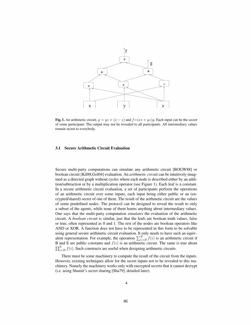
x y z

+ +

f

g

*

*

*

Fig. 1. An arithmetic circuit, g = yz + (x− z) and f=(xz + yz)g. Each input can be the secretof some participant. The output may not be revealed to all participants. All intermediary valuesremain secret to everybody.

3.1 Secure Arithmetic Circuit Evaluation

Secure multi-party computations can simulate any arithmetic circuit [BOGW88] orboolean circuit [Kil88,Gol04] evaluation. An arithmetic circuit can be intuitively imag-ined as a directed graph without cycles where each node is described either by an addi-tion/subtraction or by a multiplication operator (see Figure 1). Each leaf is a constant.In a secure arithmetic circuit evaluation, a set of participants perform the operationsof an arithmetic circuit over some inputs, each input being either public or an (en-crypted/shared) secret of one of them. The result of the arithmetic circuit are the valuesof some predefined nodes. The protocol can be designed to reveal the result to onlya subset of the agents, while none of them learns anything about intermediary values.One says that the multi-party computation simulates the evaluation of the arithmeticcircuit. A boolean circuit is similar, just that the leafs are boolean truth values, falseor true, often represented as 0 and 1. The rest of the nodes are boolean operators likeAND or XOR. A function does not have to be represented in this form to be solvableusing general secure arithmetic circuit evaluation. It only needs to have such an equiv-alent representation. For example, the operation

∑Ei=B f(i) is an arithmetic circuit if

B and E are public constants and f(i) is an arithmetic circuit. The same is true about∏Ei=B f(i). Such constructs are useful when designing arithmetic circuits.

There must be some machinery to compute the result of the circuit from the inputs.However, existing techniques allow for the secret inputs not to be revealed to this ma-chinery. Namely the machinery works only with encrypted secrets that it cannot decrypt(i.e. using Shamir’s secret sharing [Sha79], detailed later).

4

86

Aj

xi 1

xjAi

Fig. 2. A constraint between xi and xj for the desk-mates problems. An element is feasible,value ’1’, if the correponding pairs (Ai,Axi ) and (Aj ,Axj ) are allowed in a solution given thepreferences of Ai, Aj , Axi , Axj .

4 Distributed CSPs with constraints secret to everybody

In this article we redefine the distributed CSP framework, aiming to model efficiently(i.e. with a reduced search space) the distribution of some famous CSP problems,namely the stable machings problems (e.g. the desk-mates problem).

Desk-mates The desk-mates problem consists in placing a set of persons A ={A1, ..., Am} in teams of two (or two-seats desks), such that if any person Ai prefers aperson Aj to the desk-mate selected for her, then Aj prefers her current desk-mate toAi.

A way of modeling the desk-mates problem as a CSP is to have one variable xi foreach personAi specifying the index of the desk-mate assigned to her by the solution, orspecifying i, the index ofAi itself, if she remains alone. The constraints are obtained bypreprocessing the input from participants about their preferences. The fact that a personAi prefers Au to Av is specified by the first order logic predicate PAi(u, v). There isa constraint φij between every pair of distinct variables xi and xj . In first order logicnotation, the constraint between each two variables xi and xj is:

∀xi, xj : φij(xi, xj)def= (PAi(xj , xi)⇒ PAxj (j, i)) ∧ (PAj (xi, xj)⇒ PAxi (i, j)) ∧

((xi = j)⇔ (xj = i)) (1)

Read: For each pair of participants Ai, Aj , (and correspondingvariables xi and xj) there is a constraint φij that allows a pairof assignments to these variables only if:

– the fact that Ai prefers the participant assigned to Aj (Axj )to her own match Axi implies that:

the agent assigned by these assignments to Aj (Axj ),prefers the agent Aj to the agent Ai.

– the fact that Aj prefers the participant assigned to Ai (Axi )to her own match Axj implies that

the agent assigned by these assignments to Ai (Axi ),prefers the agent Ai to the agent Aj .

– Aj is the match of Ai only if Ai is the match of Aj .

5

87

Note that this model subsumes the constraints: ∀i, j : xi 6= xj . The main complica-tion with this kind of CSPs is that the constraints are functions of secrets that cannot beeasily elicited from the participants. Distributed CSP frameworks are meant to addresssuch problems.

Modeling the desk-mates problem with DisCSPs with secret constraints that are knownto some agents. One can model the desk-mates problem with secret constraints knownto some agents [ZM91,SSHF00b] by choosing as variables, x1, ..., xm, the index ofthe partner associated to each agent (that has to be computed) and using one addi-tional boolean variable for each secret preference, PAi(u, v). The total number ofboolean variables is m3, m2 of them being actually fixed by public constraints (e.g.PAi(u, u) = 0). However, also taking into account the variables x1, ..., xm, the totalsearch space becomes O(mm2m

3

). This is O(2m3

) times worse than the centralizedCSP formalization whose search space is only O(mm).

We propose now a distributed constraint satisfaction framework that allows to modelthese problems with the same search space size as the CSP framework, O(mm).

4.1 Redefining the Distributed Constraint Satisfaction Framework

In the previous part of this section we have exemplified CSP models for the stablematchings problem. We have seen that it is difficult to model efficiently these problemsusing existing private variable-, or private constraint- oriented distributed constraintsatisfaction frameworks.

Let us propose a framework for modeling distributed CSPs, where a constraint is not(necessarily) a secret known to an agent, or public, but can also be a secret unknown toall agents.

Any distributed problem is essentially (in our view) described by a set of inputs andexpected outputs from/to each participant. A distributed CSP is a specialization in thesense that the inputs are used to specify constraints/domains of a CSP, and the outputsare derived from the solution of that CSP. As shown elsewhere, sometime the inputs arealso needed (in combination with the solution) to provide meaningful outputs [Sil04b].

Definition 1. A Distributed CSP (DisCSP) is defined by six sets (A,X,D,C, I ,O) andan algebraic structure F .A={A1, ..., An} is a set of agents.X ,D, and the solution aredefined like for CSPs.

I={I1, ..., In} is a set of secret inputs. Ii is a tuple of αi secret inputs (defined onF ) from the agent Ai. Each input Ii belongs to Fαi .

Like for CSPs,C is a set of constraints. There may exist a public constraint inC, φ0,defined by a predicate φ0(ε) on tuples of assignments ε, known to everybody. However,each constraint φi, i>0, in C is defined as a set of known predicates φi(ε, I) over thesecret inputs I , and the tuples ε of assignments to all the variables in a set of variablesXi, Xi ⊆ X .

O={o1, ..., on} is the set of outputs to the different agents. Let m be the number ofvariables. oi : D1 × ... ×Dm → Fωi is a function receiving as parameter a solutionand returning ωi secret outputs (from F ) that will be revealed only to the agent Ai.

6

88

Theorem 1. The framework in the Definition 1 can model any distributed constraintsatisfaction problems with private constraints [SSHF00b].

Proof. The new DisCSP framework can be used to model any of the DisCSP problemswith constraints private to agents, by defining Ii as the extensional representation of theprivate constraint of Ai (assuming the simple but sufficient case of one constraint peragent). φi(ε, I) is then given by the corresponding value for ε in Ii (true/1 or false/0).The outputs are going to be oi(ε) = ε for all i. q.e.d.

Theorem 2. The framework in the Definition 1 can model distributed constraint satis-faction problems with private domains [YDIK98].

Proof. A private domain of an agent can also be modeled as a private unary constraint,in a DisCSP where each domain is the maximum possible domain for the variable.Then, the Theorem 1 applies. q.e.d.

We do not claim that the new framework is more general than the existing frame-works. It enables us to model naturally and efficiently the desk-mate (stable matchings)problems. One can also model these problems with the old frameworks, but they seemto yield much larger search spaces, and therefore less efficient solutions. Let us nowexemplify how this framework can model the new problems.

Modeling the desk-mates problem as a DisCSP. A way of modeling the desk-matesproblem as a DisCSP is to have one agent, Ai, and one variable, xi, for each participantin the problem description. xi specifies the index of the desk-mate assigned to Ai bythe solution, or specifies i if she remains alone. The inputs Ii of each agent are givenby the set of preferences PAi(u, v), specifying whether Ai prefers Au to Av, for eachu and v. The set F , to which belong the inputs and the outputs, is {true, false}.

There is a constraint φij between every pair of variables xi and xj , defined as in

Equation 1. The output functions are defined as: oi(ε)def= ε|{xi}. Namely, each agent

learns only the name of her desk-mate. There is a public constraint:

φ0def= ∀i, j, ((xi = j)⇔ (xj = i)) ∧ (xi 6= xj) (2)

4.2 Distributed Weighted Constraint Satisfaction Problems

Definition 2. A distributed constraint satisfaction problem (DisWCSP) is defined bysix sets (A,X,D,C, I, O), and algebraic structure F , and a set of acceptable solutionqualities B, that can be often represented as an interval [B1, B2].

– A={A1, ..., An} is a set of agents.– X = {x1, ..., xm} is a set of variables and D = {D1, ..., Dm} is a set of finite

domains such that xi can take values only from Di = {vi1, ..., vidi}. An assignmentis a pair 〈xi, vik〉 meaning that the variable xi is assigned the value vik. A tuple isan ordered set.

– I={I1, ..., In} is a set of secret inputs. Ii is a tuple of αi secret inputs (defined ona set F ) from the agent Ai. Each input Ii belongs to Fαi .

7

89

– C = {φ0, ..., φc} is a set of constraints. A constraint φi weights the legality ofeach combination of assignments to the variables of an ordered subset Xi of thevariables in X , Xi ⊆ X . φ0 is a public constraint defined by a function φ0(ε)on tuples of assignments ε, known to everybody. Each constraint φi, i>0, in C isdefined as a known function φi(ε, I) over the secret inputs I , and the tuples ε ofassignments to all the variables in a set of variables Xi, Xi ⊆ X . φi(ε, I) mapssecret inputs and tuples into weights.

– The projection of a tuple ε of assignments over a tuple of variables Xi is de-noted ε|Xi . A solution is ε∗ = argmin

ε∈D1×...×Dn

∑ci=0 φi(ε|Xi ), if

∑ci=0 φi(ε∗|Xi ) ∈

[B1...B2].– O={o1, ..., on} is the set of outputs to the different agents. oi : I×D1×...×Dm →Fωi is a function receiving as parameter the inputs and a solution, and returningωi secret outputs (from F ) that will be revealed only to the agent Ai.

Solvers developed in our previous work require that the functions in sets O and Care input either in first order logic form, or in the form of arithmetic circuits.

The inputs are not revealed to the solving machinery, as it manipulates only en-crypted data (in difference from a classic monolithic system with a trusted server).

The public constraint φ0 can be input into the system using a set of constraints{φ1

0, φ20, ...}, and the tuples of assignments accepted by φ0 can be obtained separately by

each agent, when needed, using any systematic search technique that finds all solutionsof a CSP, e.g. backtracking or lookahead algorithms (BT, BM, CBJ, FC, MAC, EMAC,etc.).

5 Adapting existing secure solvers to the new DisCSP framework

There exist a large set of algorithms addressing distributed CSPs with privacy of con-straints [Sil02,HCN+01,FMW01,WS04,YSH02b,Sil03b]. Note that none of the exist-ing techniques involves propagation, except for a very old variant in [Sil02]. The onesthat we succeed to extend to the new framework are:

– Finding the set of all solutions of a distributed constraint problem with secret con-straints [HCN+01].

– Finding the first solution in a lexicographic order for a distributed constraint satis-faction problem with secret constraints that are known to some agents [Sil03a].

– Finding a random solution for a DisCSP with secret constraints that are known tosome agents [Sil03b].

When a solution is returned to the desk-mates problem, each agentAi can infer that:any agent Ak preferred by Ai to her current desk-mate Aj , prefers her current partnerto Ai. If only one solution is returned (picked randomly among the existing solutions),then no other secret preference can be inferred with certainty.

Theorem 3. The desk-mates problem can have several solutions.

8

90

Proof. Consider a case with three agents, A1, A2, A3 where PA1(2, 3), PA2

(3, 1),PA3

(1, 2). This is a loop of preferences, and has three stable solutions, the sets of teams{(A1, A2), (A3)}, {(A2, A3), (A1)}, {(A3, A1), (A2)}. Such an example can be con-structed out of any similar loop of preferences, of any size.

If there exist several solutions, the agents will prefer not to reveal more then one ofthem. The remaining solutions would only reveal more secret preferences:

– Typically there is no other fair way, except randomness, to break the tie betweenseveral solutions.

– If the single solution that is returned is selected as the first one in some given lex-icographic order on the variables and domains of the problem, then additional in-formation is leaked concerning the fact that tuples placed lexicographically beforethe suggested solution do not satisfy the constraints [Sil03b].

As it follows, if it is known that a certain problem has only one solution, then anytechnique is acceptable among either:

– Finding and returning all solutions using the technique in [HCN+01], or– Returning only the first solution (e.g. by sequentially checking each tuple in lexi-

cographical order until a solution is found).

Otherwise, strong privacy requirements make techniques returning a random solu-tion [Sil03b] desirable, despite their potential of having a lower efficiency.

5.1 General Scheme

We will note that the main difference between the new DisCSP framework, and the onewith secret constraints that are known to some agents, is that now the constraints needto be computed dynamically from secrets inputs. All the techniques we extend to thenew framework contain a component based on Shamir’s secret sharing [Sha79]. It isthe achievement of this sharing which is most affected by the change in framework. Wewill start by describing Shamir’s secret sharing, its importance in distributed multi-partycomputations, and them we will introduce our changes.

The secure multi-party simulation of arithmetic circuit evaluation proposedin [BOGW88] exploits Shamir’s secret sharing [Sha79]. This sharing is based on thefact that a polynomial f(x) of degree t−1 with unknown parameters can be recon-structed given the evaluation of f in at least t distinct values of x, using Lagrangeinterpolation. Absolutely no information is given about the value of f(0) by revealingthe valuation of f in any at most t−1 non-zero values of x. Therefore, in order to sharea secret number s to n participants A1, ..., An, one first selects t−1 random numbersa1, ..., at−1 that will define the polynomial f(x) = s+

∑t−1i=1(aix

i). A distinct non-zero number τi is assigned to each participant Ai. The value of the pair (τi, f(τi)) issent over a secure channel (e.g. encrypted) to each participantAi. This is called a (t, n)-threshold scheme. Once secret numbers are shared with a (t, n)-threshold scheme, eval-uation of an arbitrary arithmetic circuit can be performed over the shared secrets, insuch a way that all results remain shared secrets with the same security properties (the

9

91

number of supported colluders, t−1) [BOGW88,Yao82]. For [Sha79]’s technique, oneknows to perform additions and multiplications when t ≤ (n− 1)/2. Since any bn/2cparticipants cannot find anything secret by colluding, such a technique is called bn/2c-private [BOGW88].

We do not try to encode functions, but only their inputs. All functions (more exactly,arithmetic circuits) that will be computed are public and known by all participants. Theirinputs, intermediary values, and outputs are shared secrets. The functions that we areable to compute belong to the class of arithmetic circuits. The techniques computingthese function do not reveal any information to anybody, and work by letting agentsprocessing the Shamir shares that they know, and by sharing additional secret values.

The techniques solving DisCSPs with private constraints can be used as a black box,except for the secret constraint sharing. Namely, instead of simply sending encryptedShamir shares [Sha79] of one’s constraint, those shares of the constraints have to becomputed from the secret inputs of the agents. We therefore propose to replace the secretsharing/reconstruction steps with simulations of arithmetic circuit evaluation which willcompute each φk(ε, I) for each tuple ε and for the actual inputs I . This step is calledpreprocessing. Intuitively, preprocessing is the step of computing the encrypted initialparameters of the CSP (i.e. acceptance/feasibility value of a tuple from the point of viewof each constraint), out of the provided secret inputs. Preprocessing prepares “the pairs”(y,f(y)) that encode the 0/1 values of the constraints. It is done by evaluating arithmeticcircuits.

Similarly, instead of just reconstructing the assignments to variables in a solution ε,one will have to design and execute secure computations of the functions ok(ε). Thisstep is called post-processing. Intuitively, post-processing is the step of computing theoutputs to be revealed to agents, from the obtained encrypted solution of the DisCSPand secret inputs. We show that in our cases this can also be done using simulations ofarithmetic circuit evaluations.

Assume A is some algorithm using Shamir’s secret sharing for securely findinga solution of a distributed CSP (with secret constraints known to some agents). Thegeneric extension of the algorithm A to solve the DisCSP in the new framework is:

– Preprocessing: Share the secrets in I with Shamir’s secret sharing scheme. Com-pute each φk(ε|Xk , I) for each tuple ε|Xk and for the actual inputs I by designing itas an arithmetic circuit and simulating securely its evaluation. The public constraintφ0 can be shared by any agent.

– Run the algorithmA as a black-box, for finding a solution ε∗ shared with Shamir’ssecret sharing scheme, for a DisCSP with parameters (i.e. constraints) shared withShamir’s secret sharing scheme.

– Post-processing: Compute each oi(ε∗) by designing it as an arithmetic circuit andsimulating securely its evaluation. Reveal the result of oi(ε∗) only to Ai.

5.2 Pre- and post- processing for desk-mate problems

In the remaining part of the article we will prove that it is possible to design the neededpreprocessing and post-processing to solve our example of DisCSPs, the desk-matesproblem, using the general scheme defined above.

10

92

Preprocessing for the desk-mates problem. We assume the same choice of variables, asfor the CSP formalization of this problem in Section 4. Let us now show how simplearithmetic circuits can implement the required preprocessing.

Each variable xi specifies the index of the desk-mate associated to Ai. The input ofeach agent Ai is a preference value PAi(j, k) for each ordered pair of agents (Aj , Ak),and specifying whetherAi prefersAj toAk. PAi(j, k)=1 if and only ifAi prefersAj toAk. Otherwise PAi(j, k)=0. A constraint φij is defined between each two variables, xiand xj . I.e. φij [u, v] is the acceptance value of the pair of matches: (Ai, Au), (Aj , Av).One synthesizes m(m− 1)/2 such constraints:

φi,j [u, v] =

0 when u = v

(1− PAi(v, u) ∗ (1− PAv (j, i)))∗(1− PAj (u, v) ∗ (1− PAu(i, j))) when u 6= v

The public constraint φ0 (same as in Equation 2) restricts each pair of assignments:

∀ε, ε=(〈xi, u〉, 〈xj , v)〉 : φ0(ε)def= ((u=j)⇔ (v=i)) ∧ (u 6= v)

φ0 is known by everybody, and therefore there is no need to compute it with arithmeticcircuits. The complexity of this preprocessing is O(m4) multiplications of secrets (form2 binary constraints with m2 tuples each).

The desk-mates problem does not require any arithmetic circuit evaluation for thepost-processing, as each agent Ai learns a value existing in the solution, oi(ε) = ε|{xi}.The participants just reveal to Ai their shares of xi in the solution.

6 Transforming first order logic in arithmetic circuits

Based on the experience with the examples analyzed so far, we conclude that with thenew DisCSP framework it is useful to have a mechanism for automatic translation offirst order logic sentences about secrets, into arithmetic circuits.

The main constructs in first order logic whose translation to arithmetic circuits willbe given here are: ∀i ∈ [1..n]P (i), ∃i ∈ [1..n]P (i), P ∧ Q, P ∨ Q, ¬P , minP (i)(i),and f = k, where P and Q are predicates with a true (1) or false (0) value, f is a secretinteger in a given interval, [1..n], i is a quantified variable that can take integer values ina given interval, [1..n], and k is a constant. They can also apply to variables and secretsfrom any finite set of numbers, S = {a1, ..., an}. minP (i) i is the function returningthe minimum i such that P (i) holds. The equivalent arithmetic circuits are shown inTable 1.

6.1 Complexity

For a problem with size of the search spaceΘ and c constraints, the number of messagesfor finding all solutions with secure techniques similar to the one in [HCN+01] is givenby (c − 1)Θ multiplications of shared secrets (n(n−1) messages for each such mul-tiplication). For the desk-mates problem modeled with the new framework, Θ=mm

11

93

First Order Logic Sentence Equivalent Arithmetic Circuit

P P

∀i ∈ [1..n], P (i)Qni=1 P (i)

∀a ∈ S, P (a)Qni=1 P (ai)

∃i ∈ [1..n], P (i)Pni=1[P (i)

Qi−1j=1(1− P (j))]

∃a ∈ S, P (a)Pni=1[P (ai)

Qi−1j=1(1− P (aj))]

P ∧Q P ∗QP ∨Q P + (1− P )Q

P ⇒ Q 1− P (1−Q)

¬P 1− Pf = k, (f, k ∈ [1..n])

(i.e. test if f equals k, where they are in [1..n])1

(k−1)!(n−k)!

Qk−1i=1 (f − i)Qn

i=k+1(i− f)

f = ak, (f ∈ S, k ∈ [1..n])

(i.e. test if f equals the kth element of S)

Qai∈S,i6=k(f−ai)Qai∈S,i6=k(ak−ai)

minP (i),i∈[1..n]

i

(i.e., smallest i s.t. P (i) holds)

Pni=1[iP (i)

Qi−1j=1(1− P (j))]

Table 1. Equivalences between first order logic constructs and arithmetic circuits. P and Q arepredicates and P and Q are their equivalent arithmetic circuits. S = {a1, ..., an}.

and c=1 for the version with a single global constraint, or c=m2/2 for the versionwith binary constraints. For the case with binary constraints, it yields a complexity ofO(mm+2). As mentioned before, the preprocessing has complexity O(m4) multiplica-tions between shared secrets, resulting in a total complexity O(m2(mm +m2)).

Solving the same problem with the same algorithm but modeled with the oldDisCSP framework with private constraints, Θ = mm2m

3

and c = m, for one globalconstraint from each agent. There is no preprocessing, but the total complexity isO(mm+12m

3

). The new framework behaves better since m << 2m3

. The compar-ison is similar for other secure algorithms, like MPC-DisCSP1 (see [Sil03b]) whosecomplexity is given by O(dm(c+m)Θ) multiplications between shared secrets.

Similar improvements can be achieved by applying this new framework to otherknown problems like incentive auctions and stable marriages problems [Sil04b].

7 Conclusions

DisCSPs [BMM01,SGM96,LV97,Ham99,MR99,ZWW02,BD97,FBKG02,MTSY04]are a very active research area. Privacy has been recently stressedin [MJ00,FMW01,WF02,FMG02,YSH02b] as an important goal in designingalgorithms for solving DisCSPs.

In this article we have investigated how versions of old and famous problems, stablematchings problems, can be solved such that the privacy of the participants is guaran-

12

94

teed except for what is leaked by the selected solution. Our approach uses secure simu-lations of arithmetic circuit evaluations and is therefore robust whenever no majority ofthe participants colludes to find the secret of the others, and when all agents follow theprotocol.

We note that the desk-mates problems cannot be efficiently modeled (at least not inan obvious way) with existing distributed constraint satisfaction frameworks. We havetherefore introduced a new distributed constraint satisfaction framework that can modelsuch problems with the same search space size as the classic centralized CSP models.We have shown how some techniques for the existing frameworks can be adapted toproblems modeled with the new DisCSPs, and we exemplify the model with the desk-mates problems. For m participants in the desk-mates problem, the size of the searchspace in the DisCSP model achieved with the new framework is O(mm) while theprevious framework with private constraints yields DisCSP instances with a size of thesearch space of O(mm2m

3

). In existing secure algorithms for solving DisCSPs, thenumber of exchanged messages is fix and directly proportional to the search space size,making this property of a problem instance particularly relevant.

References

[BD97] B. Baudot and Y. Deville. Analysis of distributed arc-consistency algorithms. Tech-nical Report RR-97-07, U. Catholique Louvain, 1997.

[BMM01] C. Bessiere, A. Maestre, and P. Meseguer. Distributed dynamic backtracking. In CP,page 772, 2001.

[BOGW88] M. Ben-Or, S. Goldwasser, and A. Widgerson. Completeness theorems for non-cryptographic fault-tolerant distributed computating. In STOC, pages 1–10, 1988.

[CDK91] Z. Collin, R. Dechter, and S. Katz. On the feasibility of distributed constraint satis-faction. In Proceedings of IJCAI 1991, pages 318–324, 1991.

[FBKG02] C. Fernandez, R. Bejar, B. Krishnamachari, and C. Gomes. Communication andcomputation in dis. CSP algorithms. In CP, pages 664–679, 2002.

[FMG02] B. Faltings and S. Macho-Gonzalez. Open constraint satisfaction. In CP, 2002.[FMW01] E.C. Freuder, M. Minca, and R.J. Wallace. Privacy/efficiency tradeoffs in distributed

meeting scheduling by constraint-based agents. In Proc. IJCAI DCR, pages 63–72,2001.

[Gol04] Oded Goldreich. Foundations of Cryptography, volume 2. Cambridge, 2004.[GP02] IP. Gent and P. Prosser. An empirical study of the stable marriage problem with ties

and incomplete lists. In ECAI 2002, pages 141–145, 2002.[Ham99] Youssef Hamadi. Traitement des problemes de satisfaction de contraintes distribues.

PhD thesis, Universite Montpellier II, Juillet 1999.[HCN+01] T Herlea, J. Claessens, G. Neven, F. Piessens, B. Preneel, and B. Decker. On securely

scheduling a meeting. In Proc. of IFIP SEC, pages 183–198, 2001.[IM02] R. Irving and D. Manlove. The stable roommates with ties. Journal of Algorithms,

43(1):85–105, 2002.[Kil88] J. Kilian. Founding cryptography on oblivious transfer. In Proc. of ACM Symposium

on Theory of Computing, pages 20–31, 1988.[LV97] Michel Lemaıtre and Gerard Verfaillie. An incomplete method for solving distributed

valued constraint satisfaction problems, 1997.[MJ00] P. Meseguer and M. Jimenez. Distributed forward checking. In CP’2000 Distributed

Constraint Satisfaction Workshop, 2000.

13

95

[MR99] Eric Monfroy and Jean-Hugues Rety. Chaotic iteration for distributed constraintpropagation. In SAC, pages 19–24, 1999.

[MTSY04] P.J. Modi, M. Tambe, W.-M. Shen, and M. Yokoo. Adopt: Asynchronous distributedconstraint optimization with quality guarantees. AIJ, 2004.

[SGM96] G. Solotorevsky, E. Gudes, and A. Meisels. Algorithms for solving distributed con-straint satisfaction problems (DCSPs). In AIPS96, 1996.

[Sha79] A. Shamir. How to share a secret. Comm. of the ACM, 22:612–613, 1979.[Sil02] Marius-Calin Silaghi. Asynchronously Solving Distributed Problems

with Privacy Requirements. PhD Thesis 2601, (EPFL), June 27, 2002.http://www.cs.fit.edu/˜msilaghi/teza.

[Sil03a] M.C. Silaghi. Arithmetic circuit for the first solution of distributed CSPs with cryp-tographic multi-party computations. In IAT, Halifax, 2003.

[Sil03b] M.C. Silaghi. Solving a distributed CSP with cryptographic multi-party computa-tions, without revealing constraints and without involving trusted servers. In IJCAI-DCR, 2003.

[Sil04a] M.-C. Silaghi. Secure distributed CSP solvers. http://www.cs.fit.edu/ msi-laghi/secure/, 2004.

[Sil04b] M.C. Silaghi. Incentive auctions and stable marriages problems solved with n/2-privacy of human preferences. Technical Report CS-2004-11, FIT, 2004.

[SR04] M. Silaghi and V. Rajeshirke. The effect of policies for selecting the solution of aDisCSP on privacy loss. In AAMAS, pages 1396–1397, 2004.

[SSHF00a] M.-C. Silaghi, D. Sam-Haroud, and B. Faltings. Asynchronous search with aggre-gations. In Proc. of AAAI2000, pages 917–922, Austin, August 2000.

[SSHF00b] M.-C. Silaghi, D. Sam-Haroud, and B. Faltings. Asynchronous search with privateconstraints. In Proc. of AA2000, pages 177–178, Barcelona, June 2000.

[WF02] R.J. Wallace and E.C. Freuder. Constraint-based multi-agent meeting scheduling:Effects of agent heterogeneity on performance and privacy loss. In DCR, pages 176–182, 2002.

[WS04] R. Wallace and M.C. Silaghi. Using privacy loss to guide decisions in distributedCSP search. In FLAIRS’04, 2004.

[Yao82] A. Yao. Protocols for secure computations. In FOCS, pages 160–164, 1982.[YDIK98] M. Yokoo, E. H. Durfee, T. Ishida, and K. Kuwabara. The distributed constraint

satisfaction problem: Formalization and algorithms. IEEE TKDE, 10(5):673–685,1998.

[YSH02a] M. Yokoo, K. Suzuki, and K. Hirayama. Secure distributed constraint satisfaction:Reaching agreement without revealing private information. In Proc. of the AAMAS-02 DCR Workshop, Bologna, July 2002.

[YSH02b] M. Yokoo, K. Suzuki, and K. Hirayama. Secure distributed constraint satisfaction:Reaching agreement without revealing private information. In CP, 2002.

[ZM91] Y. Zhang and A. K. Mackworth. Parallel and distributed algorithms for finite con-straint satisfaction problems. In Proc. of Third IEEE Symposium on Parallel andDistributed Processing, pages 394–397, 1991.

[ZWW02] W. Zhang, G. Wang, and L. Wittenburg. Distributed stochastic search for constraintsatisfaction and optimization: Parallelism, phase transitions and performance. InPAS, 2002.

14

96

Comparing Two Implementations of a Complete

and Backtrack-Free Interactive Configurator

Sathiamoorthy Subbarayan1, Rune M. Jensen1, Tarik Hadzic1,Henrik R. Andersen1, Henrik Hulgaard2, and Jesper Møller2

1 Department of Innovation, IT University of Copenhagen,Rued Langgaards Vej 7, DK-2300 Copenhagen S, Denmark

{sathi,rmj,tarik,hra}@itu.dk2 Configit Software A/S,

Vermundsgade 38 B, DK-2100 Copenhagen Ø, Denmark{jm,henrik}@configit-software.com

Abstract. A product configurator should be complete and backtrackfree in the sense that the user can choose freely between any valid con-figuration and will be prevented from making choices that no valid con-figuration satisfies. In this paper, we experimentally evaluate a symbolicand search-based implementation of an interactive product configurationalgorithm with these properties. Our results show that the symbolic ap-proach often has several orders of magnitude faster response time thanthe search-based approach due to the precompilation of a symbolic rep-resentation of the solution space. Moreover, the difference between theaverage and worst response time for the symbolic approach is typicallywithin a factor of two, whereas it for the search-based approach may bemore than two orders of magnitude.

1 Introduction

Product configuration involves two major tasks: to define a modeling languagethat makes it easy to specify and maintain a formal product model and todevelop a decision support tool that efficiently guides users to desirable productconfigurations [1]. In this paper we focus on the latter task and investigatea complete and backtrack-free approach to Interactive Product Configuration(IPC). The input to our IPC algorithm is a product model that consists ofa set of product variables with finite domains and a set of product rules. Avalid product configuration is an assignment to each variable that satisfies theproduct rules. The IPC algorithm initially has an empty set of user selectedassignments. In each iteration of the algorithm, invalid values in the domain ofthe variables are pruned away such that each value in the domain of a variable ispart of at least one valid configuration satisfying the existing set of assignments.The user then selects his preferred value for any free variable. The algorithmterminates when each variable in the product model is assigned a value. TheIPC algorithm is complete in the sense that the user can choose freely betweenany valid configuration. It is also backtrack-free since the user is prevented from

97

choosing a variable assignment for which no valid configuration exists. Hencethe algorithm never forces the user to go back to a previous configuration stateto explore alternative choices.

In this paper we experimentally evaluate a symbolic and search-based im-plementation of the IPC algorithm. The symbolic implementation is using atwo-phase approach [2]. In the first phase, the product rules are compiled intoa reduced ordered Binary Decision Diagram (BDD) [3] representing the set ofvalid configurations (the solution space). In the second phase, a fast specializedBDD operation is used to prune the variable domains. The worst-case responsetime only grows polynomially with the size of the BDD. Thus, the computation-ally hard part of the configuration problem is fully solved in the offline phasegiven that the compiled BDD is small. The search-based implementation prunesvariable domains by iterating over each possible assignment and searching for avalid configuration satisfying it. This approach can be improved by memorizingall assignments for which no solution exist across iterations and, within eachiteration, adding all assignments in a found solution (not just the one beingverified).

The symbolic approach has been implemented using Configit Developer 3.2

[4] that employs a BDD-derived symbolic representation called Virtual Tables(VTs). The search-based approach has been implemented using ILOG Solver 5.3

[5]. We have developed a publicly available benchmark suite called CLib [6] forthe experiments that consists of 14 configuration problems. Our results show thatthe symbolic approach often has several orders of magnitude faster response timethan the search based approach. In addition, the difference between average andworst response time is often within a factor of two for the symbolic approach,but some times more than two orders of magnitude for the search-based ap-proach. Moreover, our results indicate that the configuration space of industrialconfiguration problems often have small symbolic representations. This result issomewhat surprising since BDDs blow up for many combinatorial problems in-vestigated in AI (e.g., the n-queens problem and other permutation problems). Itmay be the frequent hierarchical structure of real-world configuration problemsthat make them particularly well-suited for BDDs.

The remainder of the paper is organized as follows. In Sect. 2, we defineproduct configuration and describe the IPC algorithm. The symbolic and search-based implementation of the IPC algorithm are described in Sect. 3 and Sect. 4,respectively. We focus on describing the symbolic implementation since we as-sume that the search-based implementation is straight forward for most readers.Section 5 presents experimental work. Finally, we describe related work in Sect. 6and draw conclusions in Sect. 7.

2 Interactive Product Configuration

We can think of product configuration as a process of specifying a product de-fined by a set of attributes, where attribute values can be combined only inpredefined ways. Our formal definition captures this as a mathematical object

98

with three elements: variables, domains for the variables defining the combina-torial space of possible assignments and formulas defining which combinationsare valid assignments. Each variable represents a product attribute. The variabledomain refers to the options available for its attribute and formulas specify therules that the product must satisfy.

Definition 1. A configuration problem C is a triple (X,D,F ), where X is a

set of variables x1, x2, · · · , xn, D is the Cartesian product of their finite domains

D1 ×D2 × · · · ×Dn, and F = {f1, f2, · · · , fm} is a set of propositional formulas

over atomic propositions xi = v, where v ∈ Di, specifying conditions that the

variable assignments must satisfy.

Each formula fi is a propositional expression inductively defined by

φ ≡ xi = v |φ ∧ ψ |φ ∨ ψ | ¬φ, (1)

where v ∈ Di. We use the abbreviation φ⇒ ψ ≡ ¬φ ∨ ψ for logical implication.For a configuration problem C, we define the solution space S(C) as the set of allvalid configurations, i.e. the set of all assignments to the variables X that satisfythe rules F . Many interesting questions about configuration problems are hardto answer. Just determining whether the solution space is empty is NP-complete,since the Boolean satisfiability problem can be reduced to it in polynomial time.

Example 1. Consider specifying a T-shirt by choosing the color (black, white,red, or blue), the size (small, medium, or large) and the print (”Men In Black”- MIB or ”Save The Whales” - STW). There are two rules that we have toobserve: if we choose the MIB print then the color black has to be chosen aswell, and if we choose the small size then the STW print (including a big pictureof a whale) cannot be selected as the large whale does not fit on the small shirt.The configuration problem (X,D,F ) of the T-shirt example consists of variablesX = {x1, x2, x3} representing color, size and print. Variable domains are D1 ={black ,white, red , blue}, D2 = {small ,medium, large}, and D3 = {MIB ,STW }.The two rules translate to F = {f1, f2}, where f1 = (x3 = MIB) ⇒ (x1 = black)and f2 = (x3 = STW ) ⇒ (x2 6= small). There are |D1||D2||D3| = 24 possibleassignments. Eleven of these assignments are valid configurations and they formthe solution space shown in Fig. 1. ♦

(black , small ,MIB) (black , large,STW ) (red , large,STW )(black ,medium,MIB) (white,medium,STW ) (blue,medium,STW )(black ,medium,STW ) (white, large,STW ) (blue, large,STW )(black , large,MIB) (red ,medium,STW )

Fig. 1. Solution space for the T-shirt example

By interactive product configuration we refer to the process of a user inter-actively tailoring a product to his specific needs by using supporting software

99

called a configurator. Every time the user assigns a value to a variable, the con-figurator restricts the possible solutions to configurations consistent with thisnew condition. The user keeps selecting variable values until only one configu-ration is left. The IPC algorithm in Fig. 2 illustrates this interactive process.In line 1, the configurator takes a given configuration problem C and compiles

IPC(C)1 R← Compile(C)2 while |R| > 13 do choose (xi = v) ∈ Valid-Assignments(R)4 R← R|xi=v

Fig. 2. The IPC Algorithm

it into an internal representation R. The procedure Valid-Assignments(R) inline 3 extracts the set of valid assignments (choices) from the internal repre-sentation. In line 4, the internal representation is restricted to configurationssatisfying the new condition. This behavior of the configurator enforces a veryimportant property of interactive configuration called completeness of inference.The user cannot pick a value that is not a part of a valid solution, and further-more, a user is able to pick all values that are part of at least one valid solution.These two properties are often not satisfied in existing configurators, either ex-posing the user to backtracking or making some valid choices unavailable. Thesymbolic and search-based implementation of the IPC algorithm differ in theirinternal representation and implementation of the valid assignment and restrictoperations.

Example 2. For the T-shirt problem, the assignment x2 = small will, by thesecond rule, imply x3 6= STW and since there is only one possibility left forvariable x3, it follows that x3 = MIB . The first rule then implies x1 = black .Unexpectedly, we have completely specified a T-shirt by just one assignment. ♦

From the user’s point of view, the configurator responds to the assignment bycalculating valid choices for undecided variables. It is important that the responsetime is very short, offering the user a truly interactive experience. The demandfor short response-time and completeness of inference is difficult to satisfy dueto the hardness of the configuration problem.

3 Symbolic Implementation of the IPC Algorithm

Since checking whether the solution space is empty is NP-complete, it is unlikelythat we can construct a configurator that takes a configuration problem andguarantees a response time that is polynomially bounded with respect to itssize. The symbolic approach is offline to compile the configuration problem to

100

a representation of the solution space that supports fast interaction algorithms.The idea is to remove the hard part of the problem in the offline phase. This willhappen if the compiled representation is small. We cannot, however, in generalavoid exponentially large representations.

3.1 Symbolic Solution Space Representation

A configuration problem can be efficiently encoded using Boolean variablesand Boolean functions. We assume that domains Di contain successive inte-gers starting from 0. For example we encode D2 = {small ,medium, large} asD2 = {0, 1, 2}. Let li = dlg |Di|e denote the number of bits required to encode avalue in domain Di. Every value v ∈ Di can be represented in binary as a vectorof Boolean values v = (vli−1, · · · , v1, v0) ∈ B

li . Analogously, every variable xi

can be encoded by a vector of Boolean variables b = (bli−1, · · · , b1, b0). Now, theformula xi = v can be represented as a Boolean function given by the expressionbli−1 = vli−1 ∧ · · · ∧ b1 = v1 ∧ b0 = v0 (written b = v). For the T-shirt examplewe have, D2 = {small ,medium, large} and l2 = dlg 3e = 2, so we can encodesmall ∈ D2 as 00 (b1 = 0, b0 = 0)) , medium as 01 and large as 10.

The translation to a Boolean domain is not surjective. There may exist as-signments to the Boolean variables yielding invalid values. For example, the com-bination 11 does not encode a valid value inD2. Therefore we introduce a domain

constraint that forbids these unwanted combinations FD =∧n

i=1(∨

v∈Dixi = v).

Furthermore, we define a translation function τ that maps a propositional ex-pression φ to the Boolean function it represents

τ(φ) :

n∏

i=1

Bli → B. (2)

The translation is defined inductively as follows

τ(xi = v) ≡ (bi = v) (3)

τ(φ ∧ ψ) ≡ τ(φ) ∧ τ(ψ) (4)

τ(φ ∨ ψ) ≡ τ(φ) ∨ τ(ψ) (5)

τ(¬φ) ≡ ¬τ(φ). (6)

Finally we can express a Boolean function representation S ′(C) of the solutionspace S(C).

S′(C) ≡ τ(FD) ∧

m∧

j=1

τ(fj). (7)

The resulting symbolic implementation of the IPC algorithm is shown in Fig. 3.In this implementation, the internal representation is a Boolean encoding Sol ofthe solution space. In order to restrict the solution space in line 4, it is conjoinedwith the Boolean encoding of the assignment chosen by the user.

101

Symbolic-IPC(C)1 Sol ← S′(C)2 while |Sol | > 13 do choose (xi = v) ∈ Valid-Assignments(Sol)4 Sol ← Sol ∧ τ(xi = v)

Fig. 3. Symbolic implementation of the IPC algorithm

3.2 Binary Decision Diagrams

A reduced ordered Binary Decision Diagram (BDD) is a rooted directed acyclicgraph representing a Boolean function on a set of linearly ordered Boolean vari-ables. It has one or two terminal nodes labeled 1 or 0 and a set of variablenodes. Each variable node is associated with a Boolean variable and has twooutgoing edges low and high. Given an assignment of the variables, the valueof the Boolean function is determined by a path starting at the root node andrecursively following the high edge, if the associated variable is true, and the lowedge, if the associated variable is false. The function value is true, if the label ofthe reached terminal node is 1; otherwise it is false. The graph is ordered suchthat all paths respect the ordering of the variables.

A BDD is reduced such that no pair of distinct nodes u and v are associatedwith the same variable and low and high successors (Fig. 4a), and no variablenode u has identical low and high successors (Fig. 4b). Due to these reductions,

u v u

x x x

(a) (b)

Fig. 4. (a) nodes associated to the same variable with equal low and high successorswill be converted to a single node. (b) nodes causing redundant tests on a variable areeliminated. High and low edges are drawn with solid and dashed lines, respectively

the number of nodes in a BDD for many functions encountered in practice is oftenmuch smaller than the number of truth assignments of the function. Anotheradvantage is that the reductions make BDDs canonical [3]. Large space savingscan be obtained by representing a collection of BDDs in a single multi-rooted

102

graph where the sub-graphs of the BDDs are shared. Due to the canonicity,two BDDs are identical if and only if they have the same root. Consequently,when using this representation, equivalence checking between two BDDs can bedone in constant time. In addition, BDDs are easy to manipulate. Any Booleanoperation on two BDDs can be carried out in time proportional to the productof their size. The size of a BDD can depend critically on the variable ordering.To find an optimal ordering is a co-NP-complete problem in itself [3], but a goodheuristic for choosing an ordering is to locate dependent variables close to eachother in the ordering. For a comprehensive introduction to BDDs and branching

programs in general, we refer the reader to Bryant’s original paper [3] and thebooks [7, 8].

3.3 BDD-Based Implementation of the IPC Algorithm

In the offline phase of BDD-based interactive configuration, we compile a BDDS(C) of the Boolean function S ′(C) of the solution space. The variable orderingof Boolean variables of S(C) is identical to the ordering of the Boolean variablesof S′(C). S(C) can be compiled using a BDD version τ of the function τ , whereeach Boolean operation is translated to its corresponding BDD operation

τ(xi = v) ≡ BDD of τ(xi = v) (8)

τ(φ ∧ ψ) ≡ Op∧(τ(φ), τ(ψ)) (9)

τ(φ ∨ ψ) ≡ Op∨(τ(φ), τ(ψ)) (10)

τ(¬φ) ≡ Op¬(τ(φ)). (11)

In the base case (8), τ(xi = v) denotes a BDD of the Boolean function τ(xi = v)as defined in Sec. 3.1. For each of the inductive cases, we first compile a BDDfor each sub-expression and then perform the BDD operation corresponding tothe Boolean operation on the sub-expressions. We have

S(C) ≡ Op∧(τ(FD), τ(f1), · · · , τ(fm)). (12)

Due to the polynomial complexity of BDD operations, the complexity of com-puting S(C) may be exponential in the size of C.

Example 3. The BDD representing the solution space of the T-shirt exampleintroduced in Sect. 2 is shown in Fig. 5. In the T-shirt example there are threevariables: x1, x2 and x3, whose domain sizes are four, three and two, respectively.As explained in Sect. 3.1, each variable is represented by a vector of Booleanvariables. In the figure the Boolean vector for the variable xi with domain Di

is (xli−1

i , · · · , x1

i , x0

i ), where li = dlg |Di|e. For example, in the figure, variablex2 which corresponds to the size of the T-shirt is represented by the Booleanvector (x1

2, x0

2). In the BDD any path from the root node to the terminal node

1, corresponds to one or more valid configurations. For example, the path fromthe root node to the terminal node 1, with all the variables taking low valuesrepresents the valid configuration (black , small ,MIB). Another path with x1

1, x0

1,

103

and x1

2taking low values, and x0

2taking high value represents two valid configu-

rations: (black ,medium,MIB) and (black ,medium,STW ), namely. In this paththe variable x0

3is a don’t care variable and hence can take both low and high

value, which leads to two valid configurations. Any path from the root node tothe terminal node 0 corresponds to invalid configurations. ♦

x1

1

x0

1

x1

2 x1

2

x0

2 x0

2x0

2x0

2

x0

3x0

3

1 0

Fig. 5. BDD of the solution space of the T-shirt example. Variable xj

i denotes bit bj

of the Boolean encoding of product variable xi.

For a BDD version of the Symbolic-IPC algorithm, each Boolean oper-ation is translated to its corresponding BDD operation. The response time isdetermined by the complexity of performing a single iteration of the procedure.All sub-operations can be done in time linear in the size of Sol except Valid-

Assignments in Line 3. This procedure can be realized by a specialized BDDoperation with worst-case complexity

O(

n∑

i=1

|Vi||Di|), (13)

where Vi denotes the nodes in Sol associated with BDD variables encoding thedomain of variable xi. As usual, Di denotes the domain of xi. For each value ofeach variable, the procedure tracks whether the value is encoded by Sol. Dueto the ordering of the BDD variables, for each variable xi, this tracking can beconstrained to the nodes Vi.

104

4 Search-based Implementation of the IPC Algorithm

Search-based approaches like SAT techniques or CSP techniques can also be usedto implement the IPC algorithm. In such cases the first step of the algorithm isto compile the configuration problem into an internal representation used by theapplied search technique. The internal representation implicitly represents theset of valid configurations. The iterative step of the IPC algorithm is repeateduntil all the variables in the product model are assigned a value. For search-basedtechniques, the procedure for calculating Valid-Assignments is theoreticallyintractable. Every time an assignment is made, propagation is applied to prunethe invalid values in the domain of all unselected variables. This can be doneby checking whether each value in the domain of all the variables has at leastone valid configuration satisfying the existing set of variable assignments. In theworst case, the search-based configurator has to find 1 −m+

∑m

i=1di solutions

for each iteration, where m is the number of unassigned variables during theiteration, and di is the domain size of the unassigned variable i during the it-eration. Improved average complexity of Valid-Assignments can be obtainedby memorizing invalid variable values. Since the solution space keeps decreas-ing, an invalid value will remain invalid in later iterations. In addition, withineach iteration, whenever the search-based IPC finds a solution, it can mark allthe assignments in the solution as valid. This can remove redundant search forsolutions.

5 Experimental Evaluation

We use Configit Developer 3.2 [4] for the symbolic implementation of the IPCalgorithm. Configit Developer has a compiler which first checks for the semanticcorrectness of the product model. If the semantics is valid, it creates a Vir-tual Table (VT) that symbolically represents all valid solutions of the productmodel. For the search-based implementation of the IPC algorithm we use ILOG

Solver 5.3 [5]. ILOG Solver is a commercial constraint programming based C++library for solving constraint satisfaction/optimization problems. In a compar-ative study, it has been shown to outperform a range of other CSP solvers [9].The source code of our benchmarks for ILOG Solver has been constructed to thebest of our knowledge. But we are not experts on the ILOG Solver technologyand there may exist more efficient implementations. ILOG Configurator [5] isanother product from the same company which uses ILOG Solver for configura-tion problems. ILOG Configurator, however, only does set bound propagation.This means that it may be possible for a user to choose assignments for whichno valid configuration exists if the ILOG Configurator is used for interactiveconfiguration.

For each configuration benchmark used in the experiments, 1000 randomrequests are generated using Configit Developer. There are several cycles of re-quests. Each cycle contains a sequence of requests in increasing order. Eachrequest consists of a set of assignments to some of the variables in the product

105

model. Each cycle of requests simulates an interactive configuration process ofa product.

All the experiments were carried out on a Pentium-III 1 GHz machine with2GB of memory, running Linux. The benchmarks used in the experiments areavailable in the CLib benchmark suite [6] in the Configit input language and theILOG Solver source language.

The results are shown in Table 1. The first column in the table lists thename of the benchmark. The second column lists the amount of CPU time inseconds used by Configit Developer for generating the corresponding VT file.The third column lists the size of the generated VT file in Kilo Bytes (KB). Asfor BDDs (see Sect. 3), the variable ordering plays a crucial role in the size ofthe VT files generated. Unless specified, the default variable order was used inthe experiments. The fourth column lists the number of solutions (#Sol) in thegenerated VT file. After generating a VT, the number of solutions representedby it can easily be counted. This is equivalent to the total number of validconfigurations for the instance. In the subsequent four columns, the CPU timefor Average response (Avg. RT) and Worst response (Wst. RT) are listed inseconds for both Configit Developer and ILOG Solver. The response times listedfor Configit Developer include the time taken for the requests generation andwriting the requests into a file. The corresponding times listed for ILOG Solveronly include the time taken for reading the requests information from the file.Requests are generated as specified above.

Table 1. Experimental Results

Virtual Table Avg. RT (sec) Wst. RT (sec)Benchmark

Time(sec) Size(KB) #Sol Configit ILOG Configit ILOG

Renault 460.00 1292 2.8x1012 0.1273 489.29* 0.240 489.29*

Bike 0.45 22 1.3x108 0.0005 1.855 0.010 882.68PC 0.89 24 1.1x106 0.0007 1.302 0.010 2.12PSR 0.38 37 7.7x109 0.0014 2.398 0.010 486.12

Parity32 13 30.00 1219 2.0x108 0.0960 0.061 0.416 0.24

Big-PC 14.82 76 6.2x1019 0.0012 0.010

v1 5.67† 253 8.2x10123 0.1620 0.320

w1 56.52† 1347 1.0x1089 0.0680 0.160

ESVS 0.25 6.7 3.5x109 0.0004 0.059 0.010 0.14FS 0.25 5.8 2.4x107 0.0003 0.036 0.010 0.21FX 0.22 5.3 1.2x106 0.0003 0.029 0.010 0.10

Machine 0.14 6.7 4.7x108 0.0004 0.009 0.010 0.03

C169 FV 2.30 (144) 287 3.2x1015 0.0134 0.195 0.010 28.77C211 FS 6.93 (957) 370 1.4x1067 0.0219 0.314 0.020 67.09C250 FW 3.22 (111) 308 1.2x1037 0.0148 0.203 0.010 38.98C638 FVK 16.53 (1980) 534 8.8x10123 0.0385 0.608 0.050 72.62

*For finding one solution only (i.e., not complete).†The variable order file has been provided by Configit Software.

106

The Renault car configuration benchmark is described in [10]. Configit De-veloper takes 460 seconds to generate the VT file containing 2.8x1012 solutionsfor the Renault instance. But ILOG Solver takes 489 seconds just to solve theproblem represented as a CSP instance. The average response time obtained forRenault by Configit Developer is 0.1273 second. Corresponding worst responsetime is 0.240 second.

The Bike and PC instances are configuration examples provided along withConfigit Developer. They represent a bike and a personal computer configurationproblem. The size of the PC and Bike instances in the Configit language is around500 and 700 lines of code, respectively. In both cases, the average response timefor Configit Developer is only a fraction of a millisecond. This is possible asthe sizes of the corresponding VT files are very small. The corresponding worstresponse time for those two instances are 10 milliseconds only. But the averageand worst response times for ILOG Solver are comparatively very high. Theworst response time for ILOG Solver in case of Bike is 882.68 seconds, whichis more than 400 times the corresponding average response time. In case of thePC example, there is not a large difference between the average and the worstresponse time of ILOG Solver. But still the values are high when compared to thecorresponding values for Configit Developer. The PSR benchmark represents apower supply restoration problem modelled as a configuration instance. Furtherdetails about this problem is available in [11]. The performance of ILOG Solverand Configit Developer on the PSR instance is similar to those obtained for theBike instance, with a large worst case response time by ILOG Solver. Parity32 13represents a parity learning problem as a configuration instance. Informationabout this problem is available in [12]. In case of the Parity32 13 problem, ILOGSolver has better performance compared to Configit Developer. The differenceis not large though. It is interesting that the VT files for Bike, PC, and PSR arecompiled faster than the corresponding average response times given by ILOGSolver.

Big-PC represents the configuration problem of a personal computer withseveral additional features than those of the previous PC instance. The v1 andw1 instances represent real configuration problems of some of the customers ofConfigit Software. They are anonymized by renaming.3 For these two instances,the corresponding variable order file was also provided by Configit Software.These instances have very large product models. For example, the Big-PC has2500 lines of code in the Configit language. The w1 instance has more than66,000 lines of code. It is very hard and error prone to convert them manually toILOG Solver code. Hence for those instances Table 1 only has results obtainedfor Configit Developer. Even though these instances represent very large productmodels, Configit Developer has fast average and worst response times.

The ESVS, FS, FX, and Machine instances are from [13]. The first three in-stances represent screw compressor configuration problems. The last one repre-sents parts of a real-world 4-wheeled vehicle configuration problem, anonymizedby renaming. These four instances are easy compared to the previous 8 instances.

3 Due to legal issues, v1 and w1 are not available in CLib.

107

This is reflected by their VT file sizes. The VT files for these instances are gener-ated in a fraction of a second. In case of the FS instance, the VT file generationtime is almost equal to the corresponding worst response time by ILOG Solver.

The last four instances are automotive product configuration problems from[14]. The original instances are in DIMACS CNF format. Good variable ordersfor these instances are obtained with the BuDDy BDD package [15] using thesift dynamic variable ordering heuristic. Configit Developer uses these variableorders for efficient VT file generation. The time taken by BuDDy to find a goodvariable order is listed in brackets in the second column of the table. For somelarge CNF files in [14], we did not do experiments as it took a lot of time tofind good variable orders. For those instances, the average response time and theworst response time given by ILOG Solver are very large.

6 Related Work

Compilation techniques have also been studied for search techniques. In [16],the authors presented Minimal Synthesis Trees (MSTs), a data structure tocompactly represent the set of all solutions in a CSP. It takes advantage of com-bining the consistency techniques with a decomposition and interchangeabilityidea. The MST is a polynomial-size structure. Operations on the MSTs, how-ever, are of exponential time complexity. This may lead to long response timesfor an interactive configurator based on MSTs.

Acyclic constraint networks and the tree clustering algorithm [17, 18] rep-resent a CSP solution space in a more compact way, organizing it as a tree ofsolved sub-problems. For extracting a solution, the generated structure offerspolynomial time guarantees in the size of the structure. The size of the sub-problems, however, cannot be controlled for all instances and might lead to anexponential blow-up. The complexity of the original problem is dominated by thecomplexity of the sub-problems, which are exponential in both space and time.Nevertheless, this is one of the first compilation approaches used to solve CSPproblems. There are efforts to cope with this exponential blow-up by additionalcompression using Cartesian product representation [19].

We are only aware of one other symbolic precompilation technique. In [10],the authors present a method which compiles all valid solutions of a configurationproblem into an automaton. After compiling the solutions into an automaton,functions required for interactive configuration, like implications, explanations,and valid-domain-calculations can be done efficiently. They also present a theo-retical view of all the complexity issues involved in their approach. They showthat all the tasks involved in an interactive configuration process are intractablein the worst case. The BDD and automata approach to two-phase interactiveconfiguration may perform equally well. A major advantage of using BDDs,however, is that this data structure has been studied intensely in formal verifi-cation for representing formal models of large systems [20, 21]. In particular, thevariable ordering problem is well studied [7]. Furthermore a range of powerful

108

software packages have been developed for manipulating BDDs [15, 22]. To ourknowledge, automata compilation has not reached this level of maturity.

Previous work comparing symbolic and search-based approaches is very lim-ited. Comparative studies of the SAT search engine zChaff [23] and BDD com-pilation show that neither approach has generally better performance than theother [24]. Similarly, a comparison of the Davis-Putnam procedure and BDDsshows complementary strengths of the two approaches rather than one dominat-ing the other [25]. For interactive configuration, though, an important advantageof the BDD approach is that it is possible to compile the solution space prior touser interaction whereas search must be interleaved with user requests.

7 Conclusion

In this paper we have compared a symbolic and search-based implementation ofa complete and backtrack-free interactive product configuration algorithm. Ourexperimental results show that the symbolic approach often has several ordersof magnitude faster response time than the search based approach due to theprecompilation of the solution space into a symbolic representation. In addition,the difference between average and worst response time is often much smallerfor the symbolic approach than for the search-based approach. Our results in-dicate that BDD-derived representations often are small for real-world configu-ration instances. We believe that this may be due to the modular structure ofconfiguration problems with a frequent hierarchical tree-like decomposition ofdependencies that BDDs are particularly well-suited for.

We are currently working on an open source C++ Library for BDD-basedinteractive configuration for research and education purposes (CLab, [26]) and acomprehensive benchmark suite of industrial configuration problems (CLib, [6]).Future work includes developing specialized BDD operations to support boththe compilation phase and interactive phase of product configuration.

Acknowledgments

We would like to thank ILOG for their elaborate answers to our user questionsfor ILOG Solver 5.3. We also thank Erik R. van der Meer for providing theT-shirt example.

References

1. Sabin, D., Weigel, R.: Product configuration frameworks - a survey. IntelligentSystems, IEEE 13 (1998) 42–49

2. Hadzic, T., Subbarayan, S., Jensen, R.M., Andersen, H.R., Møller, J., Hulgaard, H.:Fast backtrack-free product configuration using a precompiled solution space repre-sentation. In: Proceedings of the International Conference on Economic, Technicaland Organizational aspects of Product Configuration Systems, DTU-tryk (2004)131–138

109

3. Bryant, R.E.: Graph-based algorithms for boolean function manipulation. IEEETransactions on Computers 8 (1986) 677–691

4. Configit Software A/S. http://www.configit-software.com (online)5. ILOG. http://www.ilog.com (online)6. CLib: Configuration benchmarks library. http://www.itu.dk/doi/VeCoS/clib/

(online)7. Meinel, C., Theobald, T.: Algorithms and Data Structures in VLSI Design.

Springer (1998)8. Wegener, I.: Branching Programs and Binary Decision Diagrams. Society for

Industrial and Applied Mathematics (SIAM) (2000)9. Fernandez, A.J., Hill, P.M.: A comparative study of eight constraint programming

languages over the boolean and finite domains. Constraints 5 (2000) 275–30110. Amilhastre, J., Fargier, H., Marquis, P.: Consistency restoration and explanations

in dynamic CSPs-application to configuration. Artificial Intelligence 1-2 (2002)199–234 ftp://fpt.irit.fr/pub/IRIT/RPDMP/Configuration/.

11. Thiebaux, S., Cordier, M.O.: Supply restoration in power distribution systems– a benchmark for planning under uncertainty. In: Pre-Proceedings of the 6thEuropean Conference on Planning (ECP-01). (2001) 85–96

12. Parity-Function. ftp://dimacs.rutgers.edu/pub/challenge/satisfiability/

contributed/crawford/README (online)13. Tiihonen, J., Soininen, T., Niemela, I., Sulonen, R.: Empirical testing of a weight

constraint rule based configurator. In: ECAI 2002 Configuration Workshop. (2002)17–22 http://www.soberit.hut.fi/pdmg/Empirical/index.html.

14. Sinz, C., Kaiser, A., Kchlin, W.: Formal methods for the validation of auto-motive product configuration data. Artificial Intelligence for Engineering De-sign, Analysis and Manufacturing 17 (2003) 75–97 Special issue on configurationhttp://www-sr.informatik.uni-tuebingen.de/~sinz/DC/.

15. Lind-Nielsen, J.: BuDDy - A Binary Decision Diagram Package.http://sourceforge.net/projects/buddy (online)

16. Weigel, R., Faltings, B.: Compiling constraint satisfaction problems. ArtificialIntelligence 115 (1999) 257–287

17. Dechter, R., Pearl, J.: Network-based heuristics for constraint-satisfaction prob-lems. Artificial Intelligence 34 (1987) 1–38

18. Dechter, R., Pearl, J.: Tree-clustering schemes for constraint-processing. ArtificialIntelligence 38 (1989) 353–366

19. Madsen, J.N.: Methods for interactive constraint satisfaction. Master’s thesis,Department of Computer Science, University of Copenhagen (2003)

20. Burch, J.R., Clarke, E.M., McMillan, K.: Symbolic model checking: 1020 statesand beyond. In: Proceedings of the 5th Annual IEEE Symposium on Logic inComputer Science. (1990) 428–439

21. Yang, B., Bryant, R.E., O’Hallaron, D.R., Biere, A., Coudert, O., Janssen, G.,Ranjan, R.K., Somenzi, F.: A performance study of BDD-based model checking.In: Formal Methods in Computer-Aided Design FMCAD’98. (1998) 255–289

22. Somenzi, F.: CUDD: Colorado university decision diagram package. ftp://vlsi

.colorado.edu/pub/ (1996)23. Moskewicz, M.W., Madigan, C.F., Zhao, Y., Zhang, L., Malik, S.: Chaff: Engi-

neering an efficient SAT solver. In: Proceedings of the 38th Design AutomationConference (DAC’01). (2001)

24. Pan, G.and Vardi, M.Y.: Search vs. symbolic techniques in satisfiability solving. In:Proceedings of the Seventh International Conference on Theory and Applicationsof Satisfiability Testing (SAT 2004). (2004)

110

25. Uribe, T.E., Stickel, M.E.: Ordered binary decision diagrams and the Davis-Putnam procedure. In Jouannaud, J.P., ed.: Proceedings of the 1st InternationalConference on Constraints in Computational Logics. Volume 845 of Lecture Notesin Computer Science., Springer (1994)

26. Jensen, R.M.: CLab: A C++ library for fast backtrack-free interactive productconfiguration. http://www.itu.dk/people/rmj/clab/ (online)

111

BDD-based Recursive and Conditional

Modular Interactive Product Configuration

Erik R. van der Meer and Henrik Reif Andersen

Department of Innovation, IT University of Copenhagen,Rued Langgaards Vej 7, DK-2300 Copenhagen S, Denmark

{ervandermeer,hra}@itu.dk

Abstract. Interactive product configuration is a difficult problem inconstraint programming. One of the reasons for this is that interactivityrequires that the system always responds fast. One of the ways to dealwith this requirement is to adopt a two-stage approach in which a prod-uct model is compiled off-line before user interaction takes place. Onesuch approach uses reduced ordered Binary Decision Diagrams (BDDs)as the compilation target for the product model. Advantages of this rep-resentation are that it is often quite compact, that interactive configu-ration can take place in time linear of the size of the representation, andthat this size is only dependent on the solution set (the semantics) andnot on the description (the syntax) of the product model. In this paper,we extend this approach with the notion of modules, which are moreloosely coupled parts of a configuration problem that often correspondwith actual modules in the actual product. We allow for the combiningof such modules by means of shared variables, for conditional instantia-tion of such modules, and for recursion between modules which leads tomore natural descriptions of modular systems that could, in principle,be a priori unbounded in size.

1 Introduction

Interactive product configuration is often presented as an application in con-straint programming [1, 2]. One of the main problems in implementing a goodinteractive product configurator is the requirement of responding sufficientlyfast although the problem is NP-hard. Therefore, sometimes an off-line pre-computation phase is used to crack the problem so that the interactive phasecan work in time polynomial in the size of the intermediate representation [3,4]. One such approach is based on compilation to reduced ordered Binary De-cision Diagrams (BDDs), which can represent many practical solution sets verycompactly.

This is the approach we have chosen to extend. In this paper, we present theformal semantics of the pre-computation and interaction phases of the recursiveand conditional modular interactive configuration problem. In a modular con-figuration problem, each module is a configuration problem by itself, but themodules can share variables, as long as the dependency graph for the modules

112

is a directed acyclic graph, and the run-time dependency graph for the moduleinstances is a tree. In the conditional modular configuration problem, moduleinstances in the tree exist or not depending on conditions in the parent moduleinstance. In the recursive conditional modular configuration problem, the depen-dency graph for the modules is a directed graph, and the run-time dependencygraph for the module instances is a tree of unbounded but finite size.

We achieve strong guarantees on user guidance, in that all configurationis backtrack-free, while the system is sound (no invalid/inconsistent solutionsreachable), complete (all finite valid consistent solutions reachable), and ter-minable (finite valid consistent solution reachable at all times). This can beachieved in run-time linear in the number of modules. However, where in thenon-modular configuration problem the run-time can be exponential in the sizeof the original problem, the modular configuration problem can take time expo-nential in the sizes of the original modules, or time exponential in the combineddomain sizes of the shared variables. (If it did not, P = NP could be answeredaffirmatively.) However, typical configuration is very efficient.

We have implemented the configuration system described above, and arecurrently using it to model a real world modular configuration problem. Thusfar, we have studied a 2600 line model consisting of 28 modules, which compileswithin a second on a 500 MHz Pentium III, and on which user interaction ishandled without any noticeable delay. The model is not finished yet, but theBDDs seem to be growing gently as information is added. Thus far, the largestBDD found (an intermediate result during compilation) is smaller than 2000nodes. Given the strong guarantees our system provides, we believe that we areachieving good results.

2 BDD-based Modular Interactive Configuration

In the modular configuration problem, a module is an entity with variables,domains, and constraints of its own. It can be instantiated by another module,with which it then shares the variables it exports, and it can instantiate othermodules, with which it then shares the variables they export. In this way, themodule’s instances form a tree at run-time.

In programming language terms, a module can to some extent be thought ofas a class, from which objects are instantiated. Also, the usual hierarchy buildingis possible. A car can be a module, with submodules like door, roof, and engine,and each of those can in turn have submodules.

2.1 Language

Our modular configuration language has these statements:

113

module M;

export x1, ..., xn;

import M as I if C;

define x : v1, ..., vn;

ensure C;

where x is a variable name, v a value name, M a module name, I an instancename, and C a constraint satisfying the following grammar:

C ::= (C)

| !C

| C1 op C2 where op ∈ { &, |, ->, <-> }| x op v where op ∈ { <, =, >, <=, <>, >= }| x1 op x2 where op ∈ { <, =, >, <=, <>, >= }

Names are strings of alphanumerical characters, underscores and periods.The period is only used in names that refer to variables that are shared withimported modules.

An example of a single module: Here is a small t-shirt example, whichconsists of a single module:

module t shirt;

define size : small, medium, large;

define color : red, blue, black, white;

define print : save the whale, men in black;

ensure print = save the whale -> size > small;

ensure print = men in black -> color = black;

The semantics of this will be intuitively clear. However, it is interesting tonote that even though the example is trivially simple, not many people realizethat when they want a small t-shirt, everything is decided.

An example of recursion: Next, we show an example that shows a toy ap-plication for recursion; that of configuring a USB tree:

module USB;

define type : unused, scanner, printer, camera, hub;

import scanner as scanner if type = scanner;

import printer as printer if type = printer;

114

import camera as camera if type = camera;

import USB as hub connection 1 if type = hub;




This shows the power of being able to use recursion in combination with condi-tional instantiation.

An example of potential conflict: Next, we show a short example showinga potential problem with the conditionality of import. Here is module A:

module A;

define x : 0, 1, 2;

import B as b if x = 1 | x = 2;

ensure x = 1 -> b.x <= b.y;

ensure x = 2 -> b.x < b.y;

And here is module B:

module B;

export x, y;

define x : 0, 1;

define y : 0, 1;

ensure x >= y;

The point here is that, while selection of x = 1 is fine, x = 2 leads to aconflict. Therefore, 2 should be removed from the domain of variable x. Pleasenote that, since instantiation conditions can be arbitrarily large expressions, andsince conflicts can arise from any combination of modules, this is not necessarilyeasy. However, our configurator handles this correctly while maintaining fastrun-time response, stopping the user if and only if necessary.

An example of potential infinity: Next, we show a short example showinga potential problem with the recursiveness of import. Here is module A:

module A;

115

export x;

define x : 0, 1, 2;

import A if x = 1 | x = 2;

ensure x = 2 -> A.x = 2;

The point here is that, while selection of x = 1 is fine, x = 2 leads to therequirement to instantiate an infinite number of modules. Clearly, this needs tobe avoided, again by removing 2 from the domain of x. Again, this situation canoccur in more complicated ways, for example when different modules instantiateeach other recursively. In fact, the same module can even occur multiple times insuch a loop! However, our configurator handles this correctly while maintainingfast run-time response, again only stopping the user if and only if necessary.

Another example of potential infinity: Next, we show a short exampleshowing a related potential problem with the recursiveness of import. Here ismodule A:

module A;

export x;

define x : 0, 1, 2, 3, 4;

import A as a1 if x = 1 | x = 3;

import A as a2 if x = 2 | x = 4;

ensure x = 1 -> a1.x <= 2;

ensure x = 2 -> a2.x <= 2;

ensure x = 3 -> a1.x >= 3;

ensure x = 4 -> a2.x >= 3;

The point here is that, while selection of x = 0, 1 or 2 is fine, x = 3 or 4 leadsto trouble. The problem here is again one of instantiating an infinite numberof modules, only now in lock step with user choices. That is, the configuratordoes not have to instantiate an infinite number of modules right away, but theuser is doomed to keep on configuring for ever and ever. A configurator shouldavoid this, by removing the values 3 and 4 from the domain of x. Again, thisproblem can occur in more complicated forms. Still, our configurator handlesthis correctly while maintaining fast run-time response, stopping the user if andonly if necessary.

116

2.2 Main Concepts of the Semantics

Compiling a single-module configuration problem is the process of determiningthe solution set of that module, that is the set of all combinations of valuesfor the variables that satisfy the constraints. The user interaction process ofsingle-module configuration is the process of beginning with that solution space,and reducing it step by step as the user assigns values to variables. During thisprocess, we constantly keep the user informed about the remaining values thatshe can still choose for the still unassigned variables.

In modular configuration, this picture has to be extended. During modularconfiguration, there will be a tree of module instances, each of which has asolution space that we call the local solution space. Each of these will be stepwisereduced by the user, until their final configurations are found. Of course, it isnecessary for the configurator to maintain global consistency over these localsolution spaces. That is to say that each solution in a local solution space shouldbe consistent with at least one solution in each of the neighbouring moduleinstances’ solution spaces. Consistent here means that the same variables (say xin child B, and b.x in parent A) have the same values.

The global solution space is the product of all the local solution spaces. Unlikethe local solution spaces, the global solution space can also be made larger byuser selections. This happens when a user selection leads to the creation of anew instance, which introduces a new local solution space.

An instance is created when an instantiation condition in an import state-ment somewhere becomes true for all remaining solutions in the local solutionspace. In that case, it is known that for all configurations that can come out ofthe configuration process, the instance is going to be part of the global configu-ration.

There are three main things being done in the semantics. The first has todo with the propagation of variable names and domains, the second with theprevention of conflicts because of instantiation, and the third with the preventionof infinity problems.

Let us first consider the propagation of variable names and domains. Basi-cally, when a variable is exported in a module, and another module imports thatmodule, then the variable name and its domain are automatically added to theimporting module. For example, if module B exports its variable x, then moduleA which imports module B (with instance name B1, say) automatically gets avariable B1.x. Since modules can import each other recursively, and since it isalso possible for a module to export a variable it imported (say A exports B1.x),this propagation is formulated as a fixpoint operation.

Next, conflicts because of instantiation are avoided during the compilationphase: Whenever a module A imports a module B, the constraints that module Bimposes on module A when it gets instantiated are already imposed implicitly onmodule A at compile time. This ensures that any local solutions in A that wouldinstantiate B, but are not compatible with it, are removed from A’s solution set.

Finally, the possibility of infinite regression at run-time is avoided at compile-time by a second fixpoint iteration. After the modules have been compiled sepa-

117

rately (to determine their local solution spaces), the compiler starts this fixpointiteration to determine which of the local solutions of a module would allow thatmodule to be at the root of a finite subtree in the instance tree. Only thosesolutions will make it to the final solution set. The fixpoint iteration starts withthe local solutions for modules that do not instantiate any submodules, and thenadds repeatedly those local solutions for modules that only instantiate submod-ules that have compatible solutions that have already been discovered in thisfixpoint iteration.

It is important to note that our prototype configuration engine does notrepresent sets by explicit enumeration of their elements, but that it uses BDDsinstead. This makes it a lot more efficient in practice. Furthermore, during theinteraction phase, no changes are made in the BDDs, unless the user changesfocus from one module to the other, and even then changes are only made toBDDs belonging to the modules along the path between these two. This is notreadily apparent from the semantics, though.

2.3 Basic Definitions for the semantics

We now give the semantics of the modular configuration problem. These se-mantics only deal with user selections, not deselections, and they only containequivalence as a comparison operator. We do not consider these to be seriousdrawbacks, because the meaning of deselection can be given in terms of a replayof the remaining selections, and the other comparison operators can easily betranslated into a disjunctive subformula. The semantics are presented in thisway in order to keep them simpler. However, our prototype engine implementseverything directly.

We start the description of the semantics of a modular configuration problemwith some preliminary definitions. First, we define M, which is a sequence ofmodules.

M = 〈M1, . . . ,Mn〉

Then there is the addprefix function, which takes an instance name and asequence of variable names, and returns the sequence of variable names with theinstance name (and a dot) prefixed to each of them.

addprefix (instname, 〈x1, . . . , xn〉) = 〈x′1, . . . , x

′n〉

wherex′

i= instname · 〈.〉 · xi

More important is the notion of projecting a tuple of values (representing aconfiguration of a single module) onto the interface with another module.

The project function here will take a tuple in which the values are from thedomains of the variables in the sequence X, and will transform it into a tuple inwhich the values are from the domains of the variables in the sequence X’. All

118

variables in X’ must occur in X, but the reverse does not have to be the case.Note the trick with the function i, which denotes the mapping from X to X’.It is defined in the second subequation, and used in the right hand side of themain equation.

project(X,X ′, (v1, . . . , vn)) = (vi1 , . . . , vim)

where〈x1, . . . , xn〉 = X

〈xi1 , . . . , xim〉 = X ′

Finally, there are the notions of projecting a set of tuples onto a set of shortertuples, and of embedding a set of shorter tuples into a set of tuples. Theseoperations are used to project solution sets in one module onto the interface toanother, and then to embed them into the other solution domain.

Please note that projectset projects from X to X’, whereas embedset embeds

into X from X’, and that X’ should be the shorter sequence of variables of thetwo. In the case of embedset, we also need to pass in the entire domain D (the setof all valid and invalid configurations), since we need to know the full domains ofthe variables in X that do not occur in X’. S denotes a set of solutions, that is, aset of valid configurations within a module, and S’ denotes such a set projectedonto an interface.

projectset(X,X ′, S) = {project(X,X ′, V ) | V ∈ S}

embedset(X,X ′, D, S′) = {V | V ∈ D, project(X,X ′, V ) ∈ S′}

2.4 Compilation of Names

The first phase in the compilation of a modular configuration problem consists ofthe propagation of the definitions of exported variables from children to parents.Since modules can import each other recursively, this propagation is carried outas a fixpoint iteration.

The following functions obtain sequences of variable names (X), exportedvariable names (XE), and the corresponding domains (D) from (sequences of)define and export statements. Note that the domain D is not a sequence of thedomains of the separate variables, but the cartesian product of those domains.That is, it is a set of tuples, each of which represents a configuration (which mayor may not be valid.)

[[define x:v1, . . . ,vn]] = (〈x〉, {v1, . . . , vn})

[[defn1; . . . ;defnn]] = (X1 · . . . · Xn, D1 × . . . × Dn)where(Xi, Di) = [[defni]]

119

[[export x1, . . . ,xn]] = 〈x1, . . . , xn〉

[[expt1; . . . ;exptn]] = (XE1 · . . . · XE

n )whereXE

i= [[expt i]]

The next function obtains the sequence of variables and the correspondingdomain that are added to a module because of the exported variables in theimported module. The function N is used to look up the information on theimported module (N), which is a tuple, and we use the notation XN and DN toselect the X and D fields from that tuple.

[[import modname as instname if cond ]]XDN = (X,D)whereN = N (modname)X = addprefix (instname, XE

N)

D = DEN

[[impt1; . . . ;imptn]]XDN = (X1 · . . . · Xn, D1 × . . . × Dn)where(Xi, Di) = [[impt i]]XDN

Then, we define the meaning of a module (as far as names are concerned)by the following function, which takes the contributions to the variables anddomain from the different sources (local definitions, and imported definitions),and puts that information into a 4-tuple. Note that this semantic function for amodule can be seen as returning a mapping from the function N (which mapsmodule names to these 4-tuples) to a pair mapping the present module name tosuch a 4-tuple.

To examine the function more closely, the first two subequations define thelocal and imported contributions to the sequence of variable names and to thedomain. The next two subequations define the composition of this information1. The following two define what part of this information pertains to variablesthat are exported. This will be taken into account in interpreting the importingof these modules in the next fixpoint iteration. The last line, finally, constructsthe 4-tuple N .

1 The operators here are to be understood as simply composing their operands flatly,that is, not to introduce hierarchical structure.

120

[[module modname;expts;impts;defns;ensns]]XDN = (modname, N)where(XL, DL) = [[defns ]](XI , DI) = [[impts]]XDNX = XL · XI

D = DL × DI

XE = [[expts]]DE = projectset(X,XE , D)N = (X,D,XE , DE)

[[modl1; . . . ;modln;]]XDN = {P1, . . . , Pn}wherePi = [[modl i]]XDN

Finally, the meaning of a modular configuration problem posed as a sequenceof modules, is given as a function from the module names to the 4-tuples con-taining the information pertaining to variable sequences, the domains of thesemodules, and the parts of those that are exported. This function is given by:

N = µFN .[[M]]XDFN

2.5 Compilation of Solutions

The second phase in the compilation of a modular configuration problem consistsof the computation of the solution sets of all modules, and the conditions forthe instantiations of those modules. In order to maintain global consistency, andsince modules can import each other recursively, this needs to be computed bya fixpoint iteration.

We begin with the functions that obtain the subset of configurations thatsatisfy constraints (S), given the sequence of variable names and the domain:

[[ensure e]]XD = [[e]]where〈x1, . . . , xn〉 = X

[[x = v]] = {(v1, . . . , vn) ∈ D | xi = x, vi = v}[[e1 ∧ e2]] = [[e1]] ∩ [[e2]][[e1 ∨ e2]] = [[e1]] ∪ [[e2]][[¬e]] = D \ [[e]]

[[ensn1; . . . ;ensnn]]XD = (S1 ∩ . . . ∩ Sn)whereSi = [[ensni]]XD

121

Next, we have the functions that obtain the constraints coming from sub-modules (S) and the instantiation conditions for those submodules (∆). Notethe equation that defines S, which reflects the fact that constrains from submod-ules are taken into account if and only if that submodule exists. (That is, whenthe final configuration is known to be an element of C.) Also, note the functionA which we use to look up the information about the imported module.

[[import modname as instname if cond ]]S∆XDA = (S,∆)where〈x1, . . . , xn〉 = X

[[x = v]] = {(v1, . . . , vn) ∈ D | xi = x, vi = v}[[c1 ∧ c2]] = [[c1]] ∩ [[c2]][[c1 ∨ c2]] = [[c1]] ∪ [[c2]][[¬c]] = D \ [[c]]C = [[cond ]]A = A(modname)XS = addprefix (instname, XE

A)

S = (D \ C) ∪ embedset(X,XS , D, SEA

)∆ = {(C, instname,modname)}

[[impt1; . . . ;imptn]]S∆XDA = (S1 ∩ . . . ∩ Sn,∆1 ∪ . . . ∪ ∆n)where(Si,∆i) = [[impt i]]S∆XDA

Then, we define the meaning of a module by the following function. It simplylooks up the X, D, XE and DE components in N , the ∆ component follows fromthe module imports only, and the S component is taken from the constraints andthe imported modules. (Constraints from parent modules are handled at run-time.)

[[module modname;expts;impts;defns;ensns]]S∆A = (modname, A)where(X,D,XE , DE) = N (modname)SL = [[ensns ]]XD

(SI ,∆) = [[impts ]]S∆XDAS = SL ∩ SI

SE = projectset(X,XE , S)A = (X,D, S,∆,XE , DE , SE)

[[modl1; . . . ;modln;]] = {P1, . . . , Pn}wherePi = [[modl i]]S∆A

Finally, the meaning of a modular configuration problem posed as a sequenceof modules, is given as a function from the module names to 7-tuples containing

122

information about the variable sequences, domains, solution sets, instantiationconditions, and those parts of them that are relevant for the exported variables.This function is given by:

A = µFA.[[M]]S∆FA

2.6 Execution

User interaction with the configurator takes place during what we call the ex-ecution phase. At this time, the configuration problem has been compiled intothe funtion A, mapping module names to 7-tuples.

During user interaction, we will represent the configurator state by a 4-tuple(I, A,R, T ), in which T is itself a set of such 4-tuples. This is the way in whichwe represent the tree of module instances. This tree is always of finite size (theproof is beyond the scope of this paper). The other elements of the tuple are: I,which is the name of the instance; A, which is the 7-tuple that corresponds withthe module the instance was created from; and R, which is the set of remainingvalid solutions for this instance.

First, we will look at two auxiliary functions which help with instantiationand synchronization, and after that, we will look at the initial state, choices, andupdate functions that we need to operate on the configuration states.

So we begin with the first auxiliary function, which takes care of instantiationof subinstances. It takes the definition of a module (A), the remaining solutionset (R) and the current set of subtrees (T ), and returns the new set of subtrees,keeping all current subtrees, and adding all subinstances which are in the set∆A, for which the instantiation condition is satisfied, but which do not yet existin the current set of subinstances. Note that the new instances are created witha full set of solutions, and without any subinstances of their own. This task isleft to all functions that use this function. Also note that it does not take a full(I, A,R, T ) tuple as an argument - this is because the semantics turn out to beslightly less tedious this way.

subtrees(A,R, T ) = T ∪ {(I,A(M), SA(M), ∅) | (C, I,M) ∈ ∆A, R ⊆ C,∀N ∈ T.IN 6= I}

Then we continue with the second auxiliary function, which takes care of thedownward synchronization of instances in the instance tree, and of the resultinginstantiations by using subtrees. That is to say, when the solution set of aninstance is made smaller, this function can be used to ensure the consistency ofthat instance with all its subinstances, and their subinstances, and so on.

123

propagate(XP , RP , (I, A,R, T )) = (I, A,R′, T ′)whereXS = addprefix (I,XE

A)

RS = projectset(XP , XS , RP )R′ = R ∩ embedset(XA, XE

A, DA, RS)

T ′ = {propagate(XA, R′, N)|N ∈ subtrees(A,R′, T )}

We now turn to the main thrust of the semantics of execution of a modularconfiguration problem.

The first function we turn our attention to is the initialstate function. Theinitialstate function takes a module name, and returns a tuple representing aconfiguration state. This tuple is a 4-tuple representing the root instance.

initialstate(modname) = (I, A,R, T )whereI = ε

A = A(modname)R = SA

T = {propagate(XA, R,N)|N ∈ subtrees(A,R, ∅)}

Then, we turn to the operation of finding out what the choices are given a par-ticular configuration state. We have two functions for this purpose: localchoices

and globalchoices. One could consider localchoices to be an auxiliary function,as it only generates the choices for the root-instance of the tree. It is used byglobalchoices , which recursively builds up the set of possible choices for the entireinstance tree.

localchoices(I, A,R, T ) = {(x1, D1), . . . , (xn, Dn)}where〈x1, . . . , xn〉 = XA

Di = {vi | (v1, . . . , vn) ∈ R}

globalchoices(I, A,R, T ) = localchoices(I, A,R, T ) ∪ subtreechoices

wheresubtreechoices = {(IN · 〈.〉 · x,D) | N ∈ T, (x,D) ∈ globalchoices(N)}

And to finish, we consider the update functions. There are two versions. Thefirst deals with the case where a simple variable name is given, in which case thecurrent instance needs to be updated, and the change needs to be propagated tothe subinstances. The second deals with the case where the variable is a qualifiedvariable. In this case the subinstance it belongs to needs to be updated first, thenthe current instance needs to resynchronize with that subinstance, and finallyall other subinstances need to resynchronize with the current instance.

124

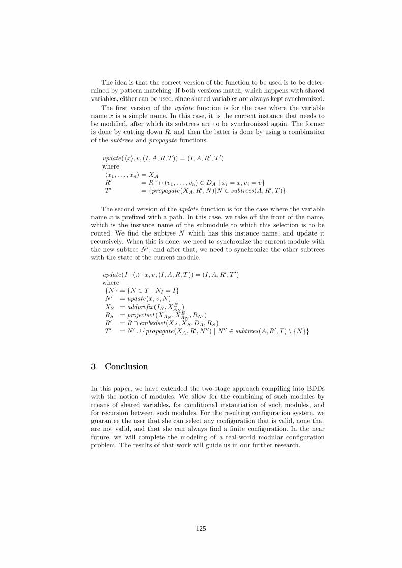
The idea is that the correct version of the function to be used is to be deter-mined by pattern matching. If both versions match, which happens with sharedvariables, either can be used, since shared variables are always kept synchronized.

The first version of the update function is for the case where the variablename x is a simple name. In this case, it is the current instance that needs tobe modified, after which its subtrees are to be synchronized again. The formeris done by cutting down R, and then the latter is done by using a combinationof the subtrees and propagate functions.

update(〈x〉, v, (I, A,R, T )) = (I, A,R′, T ′)where〈x1, . . . , xn〉 = XA

R′ = R ∩ {(v1, . . . , vn) ∈ DA | xi = x, vi = v}T ′ = {propagate(XA, R′, N)|N ∈ subtrees(A,R′, T )}

The second version of the update function is for the case where the variablename x is prefixed with a path. In this case, we take off the front of the name,which is the instance name of the submodule to which this selection is to berouted. We find the subtree N which has this instance name, and update itrecursively. When this is done, we need to synchronize the current module withthe new subtree N ′, and after that, we need to synchronize the other subtreeswith the state of the current module.

update(I · 〈.〉 · x, v, (I, A,R, T )) = (I, A,R′, T ′)where{N} = {N ∈ T | NI = I}N ′ = update(x, v,N)XS = addprefix (IN , XE

AN)

RS = projectset(XAN, XE

AN, RN ′)

R′ = R ∩ embedset(XA, XS , DA, RS)T ′ = N ′ ∪ {propagate(XA, R′, N ′′) | N ′′ ∈ subtrees(A,R′, T ) \ {N}}

3 Conclusion

In this paper, we have extended the two-stage approach compiling into BDDswith the notion of modules. We allow for the combining of such modules bymeans of shared variables, for conditional instantiation of such modules, andfor recursion between such modules. For the resulting configuration system, weguarantee the user that she can select any configuration that is valid, none thatare not valid, and that she can always find a finite configuration. In the nearfuture, we will complete the modeling of a real-world modular configurationproblem. The results of that work will guide us in our further research.

125

References

1. Sabin, D., Weigel, R.: Product configuration frameworks - a survey. IntelligentSystems, IEEE 13 (1998) 42–49

2. Tiihonen, J., Soininen, T., Niemela, I., Sulonen, R.: Empirical testing of a weightconstraint rule based configurator. In: ECAI 2002 Configuration Workshop. (2002)17–22 http://www.soberit.hut.fi/pdmg/Empirical/index.html.

3. Amilhastre, J., Fargier, H., Marquis, P.: Consistency restoration and explanationsin dynamic CSPs-application to configuration. Artificial Intelligence 1-2 (2002)199–234 ftp://fpt.irit.fr/pub/IRIT/RPDMP/Configuration/.

4. Hadzic, T., Subbarayan, S., Jensen, R.M., Andersen, H.R., Møller, J., Hulgaard, H.:Fast backtrack-free product configuration using a precompiled solution space repre-sentation. In: Proceedings of the International Conference on Economic, Technicaland Organizational aspects of Product Configuration Systems, DTU-tryk (2004)131–138

126

proceedings oft the cp-03 workshop on€¦ · · 2009-04-07proceedings of the cp 2004 workshop on...

Documents