proceedings of the seventeenth symposium on energy ...€¦ · proceedings of the seventeenth...

Proceedings of the

SEVENTEENTH SYMPOSIUM ON ENERGY ENGINEERING SCIENCES

May 13-14, 1999

ARGONNE NATIONAL LABORATORY

Argonne,Illinois

Cosponsored by

Office ofBasicEnergy Sciences

U.S. DEPARTMENT OF ENERGY

and

EnergyTechnology Division

ARGONNE NATIONAL LABORATORY

Coordinated by

Argonne National Laboratory

9700SouthCass Avenue

Argonne, IIIinois 60439


FOREWORD

This Proceedings Volume includes the technical papers that were presented during theSeventeenth Symposium on Energy Engineering Sciences on May 13-14, 1999, atArgonne National Laboratory, Argonne, Illinois. The Symposium was structured intoseven technical sessions, which included 25 individual presentations followed bydiscussion and interaction with the audience. A list of participants is appended to thisvolume.

The DOE Office of Basic Energy Sciences (BES), of which Engineering Research is acomponent program, is responsible for the long-term, mission-oriented research in theDepartment. The Office has prime responsibility for establishing the basic scientificfoundation upon which the Nation’s future energy options will be identified, developed,and built. BES is committed to the generation of new knowledge necessary to solvepresent and future problems regarding energy exploration, production, conversion, andutilization, while maintaining respect for the environment.

Consistent with DOE/BES mission, the Engineering Research Program is charged withthe identification, initiation, and management of fundamental research on broad, generictopics addressing energy-related engineering problems. Its stated goals are to improveand extend the body of knowledge underlying current engineering practice so as to createnew options for enhancing energy savings and production, prolonging the useful life ofenergy-related structures and equipment, and developing advanced manufacturingtechnologies and materials processing. The program emphasis is on reducing coststhrough improved industrial production and performance and expanding the nation’s storeof fi.mdamental knowledge for solving anticipated and unforeseen engineering problemsin energy technologies.

To achieve these goals, the Engineering Research Program supports approximately 130research projects covering a broad spectrum of topics that cut across traditionalengineering disciplines. The program focuses on three areas: (1) mechanical sciences,(2) control systems and instrumentation, and (3) engineering data and analysis. TheSeventeenth Symposium involved approximately one-fourth of the research projectscurrently sponsored by DOE/BES Engineering Research Program.

The Seventeenth Symposium was held under the joint sponsorship of the DOE Office ofBasic Energy Sciences and Argonne National Laboratory (ANL). Ms. Marianne Adairand Ms. Judy Benigno of ANL Conference Services handled local arrangements.Ms. Gloria Griparis of ANL’s Information and Publishing Division, TechnicalCommunication Services was responsible for assembling these proceedings and attendingto their publication.

I am grateful to all that contributed to the success of the program, particularly to theparticipants for their excellent presentations and active involvement in discussions. Theresulting interactions made the symposium a most stimulating and enjoyable experience.

Bassem F. Armaly, ER-15Division of Engineering and GeosciencesOffice of Basic Energy Sciences.

iv

Proceedingsofthe


May 13-14,1999

Argonne National Laboratory

Argonne, Illinois

TABLE OF CONTENTS

Technical Session I — Modeling

REPRESENTING RANDOM FIELDS WITH BIORTHOGONAL WAVELETS . . . . ...1P.D. Spanos and V.R. Rao (Rice Wziversi~)

NONLINEAR DIFFUSION AND THE PREISACH MODEL OF HYSTERESIS . . . . ...10I.D. Mayergoyz (UniversiQ of Maryland)

Technical Session II — Modeling and Diagnostics

TUNNELING CHARACTERISTICS AND LOW-FREQUENCY NOISE OFHIGH-TC SUPERCONDUCTOR/NOBLE-METAL JUNCTIONS . . . . . . . . . . . . . . . . ...17

Y. Xu and J.W. Ekin (National Institute of Standards and Technology)

AN EFFICIENT NEAR-FIELD MICROSCOPE FOR THERMALMEASUREMENTS . . . . . . . . . . . . . . . . . . . . . . . . . . . . . . . . . . . . . . . . . . . . . . . . . . . . . . . . . . 26

G.S. Kino, D.A. Fletcher, K.B. Crozier, K.E. Goodson, and C.F. Quate(Stanford University)

ELECTROMECHANICAL FRACTURE IN PIEZOELECTRIC CEWNVIICS . . . . . ...34H. Gao and D.M. Barnett (Stanford University)

THEORY OF SMALL ANGLE NEUTRON SCATTERING FROMNANODROPLET AEROSOLS . . . . . . . . . . . . . . . . . . . . . . . . . . . . . . . . . . . . . . . . . . . . . ...42

G. Wilernski (UniversiQ of Missouri — Rolls)

v

Technical Session III — Chaos and Turbulence

PHASE-DEFECT DESCRIPTION OF TRAVELING-WAVE CONVECTION . . . . . ...50C.M. Surko and A. La Porta (University of Cal~omia, San Diego)

SPATIOTEMPORAL PATTERNS IN VERTICALLY VIBRATED GIWW.JLARLAYERS: EXPERIMENT AND SIMULATION . . . . . . . . . . . . . . . . . . . . . . . . . . . . . . . ...58

M.D. Shattuck, C. Bizon, J.B. Swift, and H.L. Swinney(The University of Texas, Austin)

INSTANTANEOUS ENERGY SEPARATION IN SHEAR LAYER . . . . . . . . . . . . ,.....66B. Han and R.J. Goldstein (University of Minnesota)

Technical Session IV — Materials Diagnostics

DYNAMIC HOLOGRAPHIC LOCK-IN IMAGING OF ULTRASONIC WAVES . . ...74K.L. Telschow and V.A. Deason(Idaho National Engineering and Environmental Laboratoq)S.K. Datta (University of Colorado)

MECHANICAL BEHAVIOR AND ULTRASONIC CHARACTERIZATIONOF DUCTILE/BRITTLE LAYERED MATERIAL SYSTEMS . . . . . . . . . . . . . . . . . . . ...82

S.K. Datta, M.L. Dunn, R. Sesselmann, and J. Niklasson(University of Colorado)

MICROMECHMWCS OF MATERIALS WITH CIMCKS AND PORESOF DIVERSE SHAPES . . . . . . . . . . . . . . . . . . . . . . . . . . . . . . . . . . . . . . . . . . . . . . . . . . . . . ..90

M. Kachanov (Tuy%sUniversity)

AN INVESTIGATION OF DYNAMIC CRACK INITIATION IN DUCTILESTEELS USING HIGH SPEED INFILUIED THERMOGRAPHY . . . . . . . . . . . . .. . . ...98

A.J. Rosakis, G. Ravichandran, and P.R. Guduru(Calijomia Institute of Technology)

Technical Session V — Material Engineerin~

ORDER OF MAGNITUDE SCALING OF COMPLEXENGINEERING PROBLEMS . . . . . . . . . . . . . . . . . . . . . . . . . . . . . . . . . . . . . . . . . . . . . . .. 106

P.F. Mendez and T.W. Eagar (Massachusetts Institute of Technology)

LOW TEMPERATURE TIME DEPENDENT CRACKING . . . . . . . . . . . . . . . . . . . . ...114W.A. Van Der Sluys and J.M. Bloom (McDermott Technology Inc.)

vi

THREE-DIMENSIONAL FIWCTURE MECHANICS COMPUTATIONSUSING TETRAHEDRAL FINITE ELEMENTS . . . . . . . . . . . . . . . . . . . . . . . . . . . . . . ...122

D.M. Parks, H. Rajaram, and S. Socrate (Massachusetts Institute of Technology)

ON PREDICTING THE TRANSITION IN PROBABILITY OF IUUIECLEAVAGE IN DUCTILE CRACKED STRUCTURES . . . . . . . . . . . . . . . . . . . . . . . ...130

F.A. McClintock and D.M. Parks (Massachusetts Institute of Technology)

Technical Session VI — Materials and LiQuids

T; AND STABLE CRACK GROWTH.. . . . . . . . . . . . . . . . . . . . . . . . . . . . . . . . . . . . . . . . 138S.IV. Atluri and H. Okada (University of Cal~ornia, Los Angeles)

AN EXPERIMENTAL INVESTIGATION ON T* AS A STABLEAND FATIGUE CRACK GROWTH PARAMETER . . . . . . . . . . . . . . . . . . . . . . . . . . . . . 150

J.H. Jackson, L. Ma, P.W. Lam, and A.S. Kobayashi (University of Washington)S.N. Atluri (University of California, Los Angeles)

SPREADING ON A LIQUID INTERFACE . . . . . . . . . . . . . . . . . . . . . . . . . . . . . . . . . . . . . 158M.J, Miksis and J.J. Kriegsmann (Northwestern University)

FLOW AND HEAT TRANSFER STUDIES IN MICROSCALERECTANGULAR CHANNELS . . . . . . . . . . . . . . . . . . . . . . . . . . . . . . . . . . . . . . . . . . . . . . . 166

D. Pfund and D. Rector (Pacific Northwest National Laboratory)A. Popescu and J. Welty (Oregon State Universi~)

Technical Session VII — i14ultiphase Flow

EXPERIMENTAL MEASUREMENTS OF STRUCTURE INCONCENTRATED SUSPENSIONS . . . . . . . . . . . . . . . . . . . . . . . . . . . . . . . . . . . . . . . . . . . 174

H. Brenner (Massachusetts Institute of Technology)A.L. Graham (Texas Tech Universi~)L.A. Mondy (Sandia National Laboratories)

PINCH-OFF IN LIQUIIYLIQUID JETS: EXPERIMENTSAND SIMULATIONS . . . . . . . . . . . . . . . . . . . . . . . . . . . . . . . . . . . . . . . . . . . . . . . . . . . . . . . 184

E.K. Lmgrnire and J.S. Lowengrub (University of Minnesota)

SHEAR-INDUCED DIFFUSION OF PARTICLES IN CONCENTRATEDSUSPENSIONS . . . . . . . . . . . . . . . . . . . . . . . . . . . . . . . . . . . . . . . . . . . . . . . . . . . . . . . . . . . . 192

A. Acrivos (Levich Institute)

vii

CLOSURE OF DISPERSE-FLOW AVERAGED EQUATIONS MODELSBY DIRECT NUMERICAL SIMULATION . . . . . . . . . . . . . . . . . . . . . . . . . . . . . . . . . . . . 199

A. Prosperetti, M. Tanksley, and M. Marchioro(The Johns Hopkins University)

~NALLIST OF PARTICIPANTS . . . . . . . . . . . . . . . . . . . . . . . . . . . . . . . . . . . . . . . . . . . . 207

. ..Vlll

REPRESENTINGRANDOM FIELDSWITH BIORTHOGONALWAVELETS

P. D. SpanosL. B.Ryon Chair in Engineering

v. R. &OGraduate Student

Department of Mechanical Engineering,Rice University, Houston, TX 77005

ABSTRACT

A new method of representing random fields in a biorthogonal wavelet basis is intro-duced. It is shown that a biorthogonal basis leads to an efficient representation ofthe random process with weakly correlated wavelet coefficients. This is tantamountto an increase in decorrelation capacity of the underlying basis functions. This in-crease is shown to result from the use of a smaller number of filter coefficients ascompared to the Daubechies orthonormal family of wavelets.

INTRODUCTION

Recent developments in applied mathematics and signal processing have led to the development of

wavelet theory and its application to problems of engineering interest. Some recent applications

include the development of efficient algorithms for image processing and damage detection, for an

exhaustive review, see [9]. The discovery of a class of compactly supported wavelets by Daubechies

[6] was largely responsible for renewed interest of the engineering community in these functions.

Daubechies wavelets can be used to approximate functions with desired accuracy using only a

few significant coefficients. This [12] makes them ideal candidates for application to problems of

engineering interest [1].

It is well known that second order random processes with a positive definite covariance matrix

can be represented by means of a Karhunen-Loeve expansion. This expansion makes use of the

eigenfunctions of the covariance kernel and results in a whitened representation by the use of

uncorrelated random variables [7]. Wavelets however, are not the eigenfunctions of any operator

1

and hence cannot fully diagonalize the covariance matrix. They can however, be used to develop

an approximate KL-expansion that results in a nearly diagonal covariance matrix.

In this context, wavelets have been shown to lead to efficient represention of stochastic processes

and random fields [11, 13]. A wavelet-based KL-like expansion for wide-sense stationary random

processes has been developed by Zhang and Walter in [16], where it is shown that the covaria.nce

kernel of a widesense stationary random process can be diagonalized by a set of biorthogonal

wavelet bases obtained by starting with the Meyer wavelet. However, the resultant scaling function

and wavelet are not compactly supported in the spatial domain.

The efficacy of algorithms used to represent random processes is crucial to many problems in

stochastic mechanics. Conventional methods such as Monte-Carlo, Perturbation, and Neumann

depend extensively on such representation schemes to simulate the behavior of the systems char-

acterized by uncertainty. This is often a computationally expensive task, owing to the covariance

structure of the random field. The computational complexity can be reduced to some extent by

using the KL-expansion, as in the case of Stochastic Finite Element Method [7], where only uncor-

related random numbers need be used.

Potential applications of this study range from stochastic problems in structural mechanics

[7], fluid mechanics [5], heat transfer [10], as well as other areas where parameter uncertainty is

encountered [8]. While seeking a numerical solution to problems in these areas, it is desirable to

have a solver that computes the solution to the governing partial differential equations in.a wavelet

domain, while taking into account the multiscale representation of the parameter uncertainty. In

this paper, attention is focuses on the use of the biorthogonal spline wavelet basis to represent

random processes, which could lead to the development of efficient solution schemes for a wide

range of stochastic mechanics problems.

BIORTHOGONAL WAVELET BASES

Following the discovery of a class of compactly supported orthogonal wavelets by Daubechies

[6], a generalization to biorthogonal wavelets was proposed by Cohen, Daubechies and Feauveau

[3]. In the case of orthogonal wavelets, one set of filter coefficients {h~}, for the scaling function and

another set {g~} for the wavelets is sufficient to establish an orthogonal basis. In signal processing

and filter-bank literature [12], these filters are referred to as the quadrature mirror filters that are

used for both decomposition as well as synthesis. However, enforcing orthogonality of the wavelet

and scaling function results in a loss of symmetry for the basis functions.

Compactly supported orthogonal wavelets can nearly diagonalize certain classes of differential

operators [2]. It has been shown recently that biorthogonal wavelets built with orthogonal wavelets

as a starting point [4]are also capable of diagonalizing a class of elliptic partial differential operators.

Such operators arise in the numerical models of a number of engineering systems. The close parallels

between the wavelet representation of operators [2] and second order statistics of random processes

[15] raises the possibility of dmvloprncnt of efficient biorthogonal wmwlct schemes for problems in

stochastic mechanics.

2

,,. . . .

Extending the concepts of orthonormal wavelets [6]would require the introduction of dual MRA

given by two sequences of nested subspaces Vj and ~j such that

{o}... cv_lcvocvlc ““.P(R), {o}... cv_lcvo cvl L2(R)2(R). (1)

The subspaces ~ and ~j are spanned by translates of the primal and dual scaling functions at

scale j, given by @j,~(z) and &(z) respectively. The detail subspaces Wj and Wj are spanned by

the wavelet functions ~j,~ (x) and ~j,~ (z) respectively. The relations between the approximations

and detail subspaces (primal and dual respectively) between any two successive scales is given by

Vj+l .vj~wj and Vj+l = Vj @ Wj. (2)

The bi-orthogonality of the primal and dual MRAs can be interpreted to imply the existence

of refinement relations for the primal and dual functions ~(z), ~(z), ~(z) and ~(z), given by

(#@) = ti~ hk 4(2z – k), @) = fix k~ 7(2Z – k), (3)k k

The wavelet filter coefficients {gk} and {~k} are then given by

gk = (–l)kkfi_k_~, and, jk = (–l)kh&k_l. (5)

where M and fi are the lengths of the primal and dual scaling filters {hk} and {kk } respectively.

We note that for the case of orthogonal wavelets, the dual basis comprising of {~j,k, ~j,k} is the

same as the primal basis.

The refinement relations in Eq. (3) - Eq. (4) can be written in the Fourier domain using the

biorthogonal filter functions as

&2Ld) = mo(u)~(w), $(2U) = ?7zO(u)$(w), (6),’ I

‘1

where, the filter refinement functions m.(w), ml(w) and their dual counterparts are given as I(8)

ml(w) = ehiio(w + 7r)j fil (w) = etimo (L4J+ 7r). (9)

By virtue of the bi-orthogonality of the primal and dual subspaces, the basis functions satis& I(’#j,k, ‘h ) = ~ji~kl, (dj,k,k ) =0, (lo) ,.

(@j,k, ?i,l ) = ~ji~kl, (&k, ‘@i,/ ) =0.

3

(11)

BIORTHOGONAL WAVELET TRANSFORM

The biorthogonal wavelet transform is similar to the discrete wavelet transform of orthonormal

wavelets. Since the primal and dual basis functions constitute a basis in L2(E2), ~(z) can be

represented as

(12)

where the detail coefficients d; and d~ are the projection of the function f(z) onto the dual and

primal biorthogonal bases respectively. The detail coefficients as well as the corresponding approx-

imation coefficients are then given as

~ = (f,~j,k ) =/f (x)~j,kdx, (13)

where,

~j,k(~) = ~ ~n-2k#j+l,n(~) @j,k(~) = ~ %-2k@j+l,n(~), (15)n n

These equations relate the basis functions on the fine scale to those at a coarser scale. The

inverse relations where the fine scale coefficients are built from the coarse scale are given by

@j+l,k = ~ ~n-2k~j,n + ~ &-2k’#j,n, &j+l,k = ~ h-2k$j,n + ~ %-2k$j,n. (17)n n n n

The reconstruction in the case of an orthogonal wavelet basis involves only one set of functions.

In the case of biorthogonal wavelets however, as the regularity of primal functions can be chosen

to an an arbitrary degree, they are used in the reconstruction phase. The dual basis is used to

carry out the decomposition into the coefficients ~~ and d~. This is due to the fact that while the

primal functions are smoother, the dual functions possess more oscillations and are less regular.

On the other hand, using the smoother primal basis for the decomposition and the dual basis for

reconstruction has marked disadvantages. First, the smoother primal functions would result in a

slow decay of the coefficients. Secondly, the function reconstructed with dual wavelets would be

of low regularity. The projection is therefore carried on to a basis spanned by the dual functions

{~j,k(~)} and {ij,k(X)} to obtain the approximation and detail coefficients. Reconstruction canthen be carried out using these coefficients with the primal basis functions {@j,k(z) } and {oj,k(~)}.

As a consequence of the imposed vanishing moments, the dual functions are more oscillatory

in nature, and less regular than the primal functions. In particular, increased regularity of the

4

wavelet @(z) requires additional vanishing moments for the dual wavelet function @(z). However,

there need be no regularity conditions on ~(x), which satisfies the relation

/2+j(z) (h = o, k=Ol ~.9 9...? (18)

This is equivalent to requiring that the Fourier transform fil (u) of the dual wavelet filter {ijk}

have a zero of A@ order at w = O, or that me(o) be divisible by (1+ e-ti)~.

The biorthogonal wavelet transform can be then obtained by substituting the refinement rela-

tions for ~(~) and ~(z) in Eq.(4) into Eq.(13) and Eq.(14). Then, a biorthogonal equivalent of the

classical Mallat’s Pyramidal algorithm for functional decomposition is obtained. Carrying out the

above substitutions results ‘in the following expressions for the coefficients ~k and d~ at scale j in

terms of coefficients at the next finer scale -j+ 1.

(19)

The complete biorthogonal wavelet transform of a function represented by NJ samples therefore

involves successively decomposing each approximation vector Cj, and is a 0 (Nf) algorithm.

BIORTHOGONAL SPLINE WAV13LETS

B-Splines, being analytically defined functions are ideal choice for wavelets when used to recon-

struct functions. However, while B-splines of order n are refinable, their translates do not satisfy

the orthonormality condition essential for their use as orthonormal basis functions. Cohen et al.

[3] show that for any B-spline of order M, there exist many dual functions of order fi.

The scaling function ~(~) of a B-spline of order A4 can be obtained by repeated convolutions

of the box-function on [0, 1]. Alternatively, the A@ derivative of ~(z) is defined by a series of the

Fourier transform of its corresponding filter coefficients as

rno(2u) = e-iw (COSW)M, (20)

where, K = O for M even, and 1 for M odd. This is due to the fact that for M even, the primal

and dual scaling functions, ~(z) and J(z) are symmetric about z = O, while those for Al odd are

symmetric about x = 1/2, The corresponding wavelets ~(x) and J(z) are always centered about

x = 1/2 and are symmetric for M even, antisymmetric for M odd. The dual scaling filter ho(w)

corresponding to the frequency response of the filter {fik } is given by the equation

- K–17720(2w) = e–iW (cosw)M ~ C~-l+n (sinw)2n. (21)

nao

For a given primal scaling function of order M and dual scaling function of order fi, there can

be many dual wavelet functions, all of which satisfy the condition itl + fi = 2K, such that fi >1.

This condition is related to the symmetry that is retained by the biorthogonal basis functions, a

property lacked by Daubechies wavelets.

RANDOM FIELD REPRESENTATION

The expressions for the second order statistics of the scaling function and wavelet coefficients have

been discussed at length in [15] for the case of Daubechies wavelets. The goal of this section is to

investigate the decay of the wavelet coefficients in a biorthogonal basis. These correlations between

approximation coefficients ~~ and detail coefficients d; assuming that the dual functions are used

to carry out the representation, are given by the following three relations

(22)

(23)

(24)

The above integrals can be evaluated recursively using the refinement relations for ~(z) and

~(z) in Eq.(3) and (4). These integrals then can be evaluated in O(N log N) and O(N) operations

for non-stationary and stationary processes respectively as shown in [15]. Further speed.up can be

obtained when coiflets with vanishing moments equally distributed between the scaling function and

wavelet are used, resulting in 0(N) operational algorithms in the case of non-stationary processes.

However, since the support for the coiflets increases with additional vanishing moments imposed

on the scaling function, the increase in speedup is offset by increasing filter lengths. (Coiflets with

M vanishing moments on the wavelet and M – 1 moments for the scaling function have a support

length 6M – 1, as opposed to 2M – 1 for an equivalent Daubechies wavelet with M vanishing

moments.)

The expressions

VARIANCE OF WAVELET COEFFICIENTS

for the variance of wavelet coefficient correlations can be derived, from the

relations in Eqs. (22) to Eq. (24) by using the appropriate refinement relations for the dual functions.

In particular, we look at at the correlation of the scaling function coefficients a~, given in Eq.(24).

This equation can be rewritten using the moments of the dual scaling function by making a change

of variable vi = ~i — 2–~k, i = 1,2, and then expanding the autocorrelation funci,ion about

(YI, Y2) = 2–j (k, 1). This yields the following expansion, assuming that that the autocorrelation

function is atleast Q times differentiable.

(25)

,

where,

6

(26)

all

M

For sufficiently large j, or in other words, for a fine enough scale, the leading term dominates

other terms by a factor of 2–~, owing to the normality of the dual functions. Hence

. .a~-j x 2–@(2-~k, 2–~1). (27)

Carrying out a similar exercise with the dual wavelet (with Al vanishing moments such that

~ Q) for the correlation coefficients d~~ leads to the result that

(28)

Note that the nature of the above ratio is the same as obtained for Daubechies Wavelets rep

resentation of random processes [14]. However, the dual basis offers more flexibility due to the

relaxation of the condition of orthonormality.

CROSS-SCALE CORRELATIONS

The cross-scale correlations for the general case of non-stationary random processes can be

computed using the expressions in Eqs. (22) to (24). It is possible to obtain upper bounds for these

coefficients in the the case of stationary random processes, In particular, it can be shown that the

cross-scale correlation obtained from low order splines shows a decay which is better than that

obtained with high order Daubechies wavelets. This decay is related to the function xk (u), given

by the equation

Xk(w) = ‘2-j/2+2 - ~

k–1

17n@)l.@,(2kL41. l-J I?7U-J(2L4] (29)j=(l

An upper bound for cross-scale correlation of wavelet coefficients is given by the relation

(30)

It is evident horn the above equations that the function Xk(ti) determines to a large extent the

magnitude of ~k~~across scales. Therefore, xk (u) will hereafter be referred to as the de-correlation

function.

CONCLUSIONS

Based on the studies carried out in the preceding sections, it maybe surmised that biorthogonal

wavelets are better than Daubechles orthogonal wavelets in representing random fields. This is due

to the increased de-correlation capacity of the dual wavelets in a biorthogonal basis. It has been

found that increasing the number of vanishing moments on the dual wavelet lead to a faster decay

of the wavelet correlation across scales through attenuation of the peaks of the function xk (u) in

Eq.(29). It has also been observed that for a given order of the primal wavelet, there is a limiting

7

,

order of the dual wavelet beyond whkh the correlation cannot be weakened any further. This is

due to the fact that for increasing order of the dual wavelet, the basis functions become smoother

without any further qualitative changes in their appearance. Hence their approximation properties

change only marginally. This feature is also reflected in the variance of the resulting wavelet and

scaling functions across scales, which is nearly the same for wavelets of increasing dual order. This

implies that a low order dual wavelet can be adequate for representing the random process if the

tolerance levels on the correlation across scales are not too strict.

The de-correlation function defined in Eq.(29) is shown in Fig. for Daubechies wavelets with

M = 1 (Haar wavelets) and for Biorthogonal wavelets with M = 1, fi = 5. It can be seen from

these figures that the cross:scale correlation will decay faster in the biorthogonal case, in light of

Eq.(30). This decay can be attributed to the

function in u G [0 7r].

attenuation of trailing hills of the de-correlation

IdX (O’X

Figure 1: ~e-correlation function from Daubechies wavelets (M = 1) versus Bi-orthogonal wavelets(M= 1,M = 5). Tne number of scales used is given by k.

References

[1]

[2]

[3]

[4]

[5]

K. Amaratunga, J.R. Williams, S. Qian, and J. Weiss. Wavelet-galerkin solutions for one-dimensions.1partial differential equations. Int. J. Num. Meth. Eng., 27:2703-2716, 1994.

G. Beylkin. On the representation of operators in bases of compactly supported wavelets.SIAM Journal of Numerical Analysis, 6(6):1716-1740, 1993.

A. Cohen, I. Daubechies, and J.-C. Feauveau. Biorthogonal bases of compactly supportedwavelets. Comm. Pure and AppL Math., 45:485–560, 1992.

S. Dahlke and I. Weinreich. Wavelet-Galerkin methods: An adapted biorthogonal waveletbasis. Constructive Approximation, 9:237-262, 1993.

M.P. Dainton, M.H. Goldwater, and N.K. Nichols. Direct computation of stochastic flow inreservoirs with uncertain parameters. Journal of Computational Physics, 130:203–2!16, 1997.

,.

8

. .:.

[6] ~..~$i;;l.s~;t~~;mal bases of compactly supported wavelets. Comm. Pure and Appl...9 . > .

[7] R. G. Ghanem and P. D. Spanos. Stochastic Finite Elements: A Spectral Approach. Springer-Verlag, 1991.

[8] J. Glimm and D. Sharp. Stochastic partial differential equations: Selected applications incontinuum physics. Technical Report Preprint # SUNYSB-AMD-96-24, University of StonyBrook, Stony Brook, NY 11794, 1996.

[9] B. Jawerth and W. Sweldens. An overview of wavelet based multiresolution analyses. SIAMRev., 36(3):377-412, 1994.

[10] G. D. Manolis and R. P. Shaw. Boundary integral formulation for 2D and 3D thermal problemsexhibiting a linearly varying stochastic conductivity. Computational Mechanics, 17:406-417,1996.

[11] P.D. Spanos and B.A. Zeldin. Wavelets concepts in stochastic mechanics. Submitted to Prob-abilistic Engineem”ngMechanics, 1997. Preprint, Department of Mechanical Engineering, RiceUniversity.

[12] G. Strang and T. Nguyen. Wavelets and Filierbanks. Wellesley-Cambridge Press, 1996.

[13] P.W. Wong. Wavelet decomposition of harmonizable random processes. IEEE Trans. Infor-mation Theo~, 39(1):7–18, January 1993.

[14] B.A. Zeldin and P. D. Spanos. Random field representation and synthesis using wavelet bases.lkans. ASME Journal of Applied Mechanics, 63:946-952, 1996.

[15] B.A. Zeldin. Representation and synthesis of random fields : ARMA, Galerkin, and waveletprocedures. PhD thesis, Rice University, Houston, Texas, 1996.

[16] J. Zhang and G. Walter. A wavelet-based KL-like expansion for wide-sense stationary randomprocesses. IEEE Trans. on Signal Processing, 42:1737-1745, 1994.

NONLINEAR DIFFUSION AND THE PREISACH MODELOF HYSTERESIS

I.D. Mayergoyz

Electrical Engineering DepartmentUniversity of Maryland, College Park, MD 20742

ABSTRACT

It is shown that, in the case of abrupt (sharp) magnetic transitions, eddy currenthysteresis can be represented in terms of the classical Preisach model. In this represen-tation, memory effects are taken into account by the structure of the Preisach model,while dynamic effects are accounted for by a special form of the input to the model.A startling consequence of this representation is the fact that nonlinear dynamic eddycurrent hysteresis can be fully characterized by its step response.

INTRODUCTION

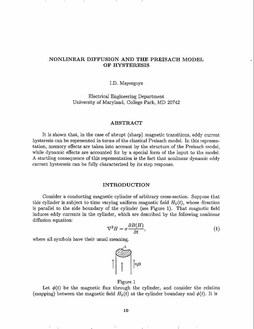
Consider a conducting magnetic cylinder of arbitrary cross-section. Suppose thatthis cylinder is subject to time varying uniform magnetic field Ho(t), whose directionis parallel to the side boundary of the cylinder (see Figure 1). That magnetic fieldinduces eddy currents in the cylinder, which are described by the following nonlineardiffusion equation:

V~H = /B(H)at ‘

(1)

where all symbols have their usual meaning.

L

n

Ill~(t)

Figure 1Let @(t) be the magnetic flux through the cylinder, and consider the relation

(mapping) between the magnetic field Ho(t) at the cylinder boundary and ~(t). It is

10

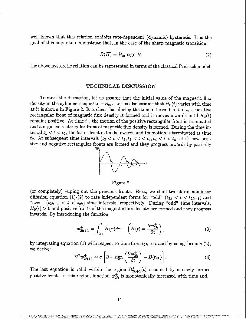
well known that this relation exhibits rate-dependent (dynamic) hysteresis. It is thegoal of this paper to demonstrate that, in the case of the sharp magnetic transition

B(H) = Bm sign H, (2)

the above hysteretic relation can be represented in terms of the classical Preisach model.

TECHNICAL DISCUSSION

To start the discussion, let us assume that the initial value of the magnetic fluxdensity in the cylinder is equal to –Bm. Let us also assume that Ho(t) varies with timeas it is shown in Figure 2. It is clear that during the time interval O < t < tl a positiverectangular front of magnetic flux density is formed and it moves inwards until Ho (-t)

remains positive. At time tl, the motion of the positive rectangular front is terminatedand a negative rectangular front of magnetic flux density is formed. During the time in-terval fl < -t < t2, the latter tkont extends inwards and its motion is terminated at timet2. At subsequent time intervals (t2 < -t < t3, t3 < t < t4,t4 < t < t5, etc.) new posi-tive and negative rectangular fronts are formed and they progress inwards by partially

HJ),

Figure 2

(or completely) wiping out the previous fronts. Next, we shall transform nonlineardiffusion equation (l)-(2) to rate independent forms for “odd” (t2k < t < t2k+1) and“even” (t2k–1 < t < t2k) time intervals, respectively. During “odd” time intervals,Ho(t) >0 and positive fronts of the magnetic flux density are formed and they progressinwards. By introducing the function

It

( 6’W+W;-+l = H(r)dr,

)H(t) = & ,

tzk(3)

by integrating equation (1) with respect to time from t2k tot and by using formula (2),we derive:

(4)

The last equation is valid within the region fl~k+l (t) occupied by a newly formed

positive front. In this region, function w~k is monotonically increased with time and,

()~consequently, sign at = 1. In the same region, we also have .B(t2~) = –Bm. As a

result, equation (4) takes the form of the Poisson equation:

V2w$/+1 = 20B7n (5)

The solution of the last equation is subject to the following boundary conditions:

It

Wk+l(ok = wJ2k+l(~) = i%)(r)dr, (6)tzk

(7)

(8)

where v is a normal to the moving boundary L~~+l (t) of the region fl~~+l (t).

Boundary conditions (7) and (8) at the moving boundary L~_+l (t) follow from thefact that magnetic field and tangential component of electric field are equal to zero atthe points of L~~+l (t) for the time interval tz~ < I- < t, that is, before the arrival ofthe positive front.

During “even” time intervals, Ho(t) <0 and negative fronts of the magnetic fluxdensity are formed and they extend inwards with time. By introducing the function

/

tW;k = H(r)dr,

tzk-1

and by literally repeating the same line of reasoningfollowing boundary value problem:

v2w;k = –h-%,

(9)

as before, we end up with the

(lo)

rt

W;k(t) IL = wl),z~(t) =I

Ho(~)d~, (11)t2k_l

w-k (-0IL;k(t)= o> (12)

aw;k~lL;k(t) = 0. (13)

The following properties can be inferred by inspecting boundary-value problems (5)-(8)and (10)-(13).

Rate Independence Property.Boundary value problems (5)-(8) ‘and (10-13) are rate independent. Consequently,

the instantaneous positions and shapes

determined by instantaneous boundary

of moving boundaries L~~+l (t) and L&(t) are

values of w~2~+1 (t) and w~zk (t), respectively.

12

Symmetry Property.Boundary value problems (5)-(8) and (10)-(13) have identical (up to a sign) math-

ematical structures. This suggests that, if lzu~zkI = Iw~zk+l 1, then the corresponding

boundaries L;k and L~k+l are identical. In other words, there is complete symmetry

between inward motions of positive and negative fronts.Now, we introduce the function:

1t

W()(t) = Ho (r)dr.o

(14)

It is clear that function W. (t) is a sum of the appropriate functions w~z~ (t) and W~2k(t).It is also clear that W. (t) achieves local maxima at t = t2~+1 and local minima at t = t2~.Next, we intend to show that ~(t) vs. W.(t) is a rate independent hysteretic relation.The rate independence of the above relation directly follows from the previously statedRate Independence Property. It is also true that ~(t) vs. W. (-t) is a hysteretic relation.Indeed, the current value of ~(t) depends not only on the current value of W. (-t) but onthe past extremum values of W. (t) as well. This is because the past extremum valuesof W.(t) determine the final locations and shapes of positive and negative rectangularfronts of II that were generated in the past. These past and motionless rectangularfronts affect the current values of ~(t). It is also apparent that there are reversals of

~(t) at extremum values of W. (t). In other words, new branches of @ vs. W. relationare formed after local extrema of W.(t). The previous discussion clearly suggest that@ vs. W. is a rate independent hysteretic relation. Next, we shall demonstrate thatthis hysteretic relation exhibits the wiping-out and congruency properties. Indeed,every monotonic increase (or decrease) of w (t)results in the formation of a positive (ornegative) rectangular front of the magnetic flux density, which extends inwards. Thismoving front will wipe out those previous rectangular fronts if they correspond to thoseprevious extremum values of W.(t), which are exceeded by a new extremum value ofW.(t). In this way, the effect of those previous extremum values of W.(t) on the futurevalues of magnetic flux d(t) is completely eliminated. This means that the wiping-out

property holds [1]. Now, we shall demonstrate the validity of the congruency property.

Consider two different boundary conditions: W$) (t) and W$’)(t). Suppose that W$) (t)

and W$) (t) have different past histories (different past extrema) but, starting hornsome instant of time, they vary monotonically back-and-forth between the same twoextremum (reversal) values. It is apparent that the above back-and-berth variations

of W$) (t) and w~) (t) will affect in the identical way the same surface layers of theconducting cylinder. Consequently, those variations will result in equal incrementsof the magnetic flux, which is tantamount to the congruency of the correspondingminor loops. Since the wiping-out and congruency properties constitute necessary andsufficient conditions for applicability of the Preisach model ([1], [2]), we conclude thatthe @vs. W. relation can be represented by the Preisach model. As a result, we arrive

at the following representation of eddy current hysteresis:

(15)

It is worthwhile to stress two remarkable points related to the above result. First,memory effects and dynamic effects of eddy current hysteresis are clearly separated.The memory effects are taken into account by the structure of the Preisach model,

while the dynamic effects are accounted for by the nature of the input (~~ .Ho(~)cZ~)

to this model. Second, the last formula suggests that the Preisach model can be usefulfor the description of hysteresis exhibited by spatially distributed systems. This is incontrast with the traditionally held point of view that the Preisach model describesonly local hysteretic effects in magnetic materials.

Next, we turn to the discussion of properties of function p(~, @ in formula (15).By using the symmetry Property, it can be inferred that the same increments ofW.(t), occurred after different extremum values of W.(t), result in the sameincrements of ~(t). This fact implies that the integral

F(%~)= // P(CY’,fl’)dcid~’ (16)

T(c@)

over a triangle T(cr, ~), defined by inequalities a! < ~, /3’ > ~, c$ – @ ~ O, does notdepend on a and ~ separately but rather on the difference a – ~. In other words,the value of the above integral is invariant with respect to parallel translations of thetriangle T(Q, @ along the line cr = ~. This is only possible if

p(a, /3) = /J(cl – ~). (17)

This means that function p assumes constant values along the lines a – ~=const. Byusing formula (17), it can be established that function p can be found by measuringonly the ascending (or descending) branch of the major loop of @ vs. W. hystereticnonlinearity. It can also be shown that any path traversed on (w., @) plane is piecewisecongruent to the ascending branch of the major loop. Thus, @ vs. W. hystereticnonlinearity is completely characterized by the ascending branch of the major loop.This branch can be found experimentally by measuring the step response of eddy

current hysteresis. Indeed, by assuming initial condition 13(0) = –.Elm and by applyingthe field HO(t) = 1, we can measure flux ~(t), which corresponds to We(t) = t. Byexcluding time t, we find the function @(wo), which describes the ascending branch ofthe major loop. Thus, we arrive at the remarkable conclusion that nonlinear (anddynamic) eddy current hysteresis can be fully characterized by its stepresponse.

14

Formula (15) can be generalized to the case when abrupt (sharp) magnetic tran-sitions are described by rectangular hysteresis loops (see Figure 3). It can be shownthat in that case formula (15) can be modified as follows:

d(~)= ///4u3)%(/”WO(WT) Ckdp,o

Op

(18)

where function A(iYo) is defined as:

A(H))= (Ho – HC)S(HO – H.) + (Ho+ H.) S(–HO – H.), (19)

and s(.) is the unit step function.

We conclude this paper with an elegant derivation of the formula for the front Z. (t)in the case of plane boundary, that is in lD case. In that case, the boundary-valueproblem (5)-(8) is reduced to:

d2w— = 20Bm,dzz if O < z < .zo(t), (20)

/

t

W(o, t) = Wl)(t) = Ho(r)dr, (21)o

dw(z, t)W(zo(t), t) = o,

dz Izo(t)= 0. (22)

B

+P-%

-H Hc H

-B~

Figure 3

The solution to equation (20), which satisfies the boundary condition (21) andsecond boundary condition (22) is given by:

w(,z, t) = CTBmZ2 – 2cBmzzo (t) + Wo (t). (23)

To find Z.(t), we use the first boundary condition (22), which leads to:

–cBmz; (t) + We(t) = O. (24)

The last expression yields:

15

(25)

This is the well known formula that can be traced back to the paper of W. Wolmanand H. Kaden [3].

ACKNOWLEDGEMENT

This work has been supported by the U.S. Department of Energy.

REFERENCES

1. I.D. Mayergoyz, “Mathematical Models of Hysteresis”, New York, Springer-Verlag,1991.

2. I.D. Mayergoyz, Phys. Rev. Let., 56, No. 15, 1986, 1518-1521.

3. W. Wolman and H. Kaden, Z. Techn. Phys., 13, 1932, 330-345.

16

TUNNELING CHARACTERISTICS AND LOW-FREQUENCY NOISEOF

HIGH-77C SUPERCONDUCTOR/NOBLEMETAL Junctional

Yizi Xu and J. W. Ekin

National Institute of Standards and TechnologyBoulder, Colorado 80303, U.S.A.

ABSTRACT

We report extensive measurements of transport characteristics and low-frequency resistance noise of c-axis YBCO/Au junctions. The dominant conduc-tion mechanism is tunneling at low temperatures. The conductance characteristicis asymmetric, and the conductance minimum occurs at a non-zero voltage. Thesefeatures can be qualitatively explained by modeling the YBCO/Au interface witha Schottky barrier. The model shows the YBCO surface behaves like a p-typesemiconductor, with a Fermi degeneracy of about 0.1 eV. This is consistent witha carrier density of 3 x 1021cna-3, and a band mass of 2.6 times that of the freeelectron mass. The barrier-height is approximately 1.0 eV. We show that interfacestates and disorder play an important role in determining the conductance charac-teristics. Low-frequency noise measurements of many junctions with contact areasranging from 4 pm2 to 64 pm2, over a wide temperature and bias range, indicatethat the noise figure for engineering design may be expressed as a normalizedresistance fluctuation &R/R = 6 x 10–4 /@ at 10 Hz.

INTRODUCTION

The YBCO/Au interface plays an important role in many high-TC electronics applications.For example, the electrical and mechanical properties of this interface determine the integrityof Au wire-bond contacts to YBCO thin film devices, which determines the reliability of devicepackaging. In another application, YBCO thin films are used to make detection coils in low-field Ma~etic Resonance Imaging (MRI) systems. The use of high-TC superconductors offersincreased signal-to-noise ratio, enabling low-field MRl systems. It is therefore very importantthat the contacts to the YBCO detection coils be both low-resistance and low-noise in order notto compromise the benefits of using these superconductors.

1Contribution of NIST, not subject to copyright.

17

The success of these applications requires an understanding of the physical mechanism ofconduction across the YB CO/Au interface. The purpose of this work is to gain such an under-standing. In this paper we first report our extensive measurements of transport characteristicsof YBCO/Au junctions. We then present a simple model for our results. Finally we presentlow-frequency resistance noise data of our junctions, which are of important technological valueand also provide insight for understanding YBCO/Au interfaces.

FABRICATION AND CONDUCTANCE MEASUREMENT

The YBCO thin films used in this work were prepared using the pulsed laser depositiontechnique. The films were c-axis orientated, with TC in the range of 87 to 91 K. We patternour films using standard photolithography. One unique feature in our process is the use of aninsulating layer of MgO to define small contact areas, which varied fi-om 2x 2 pm2 to 16x 16 pm2.The current flows nominally along the c-axis of YBCO, through a native tunnel barrier, intothe Au electrode. The native tunnel barrier was formed on the surface of the c-axis orientatedYBCO film during the fabrication process, and is thought to consist of adsorbed impurities, aswell as the degraded top-most atomic layers of the YBCO film. Electrically, the native tunnelbarrier behaves as a thin insulating or semiconducting layer between the superconductor (YBCO)and normal metal (Au). The dominant conduction mechanism of such junctions is tunnelingat low temperatures. The low-temperature tunneling resistance of our junctions with difFerentareas ranged from a few ohms to a few hundred kilohms. We developed a system for measuringjunction current vs. voltage characteristics and its first derivative with high resolution and dataacquisition rate. The details of our junction fabrication and measurement techniques can befound elsewhere [1].

A typical low-temperature conductance vs. voltage curve for our junctions is shown inFig. 1. Note that the curve is asymmetric: the incremental conductance (i.e., dI/dV) at aforward bias, when the Au-electrode is biased positively with respect to the YBCO-electrode,is greater than the corresponding reverse bias. The low bias range, shown in more detail inthe inset, is characterized by the following features: (A) a zer~bias conductance peak, (B) forvoltages less than about 30 mV the conductance is conspicuously lower than that extrapolatedhorn the high bias range (the dashed line in the inset), (C) a conductance minimum at a reversebias (Vmin in the inset), which would be apparent if the features in (A) and (B) were suppressed.

There has been considerable controversy surrounding the issue of the zero-bias conductancepeak (ZBCP) in YBCO/noble-metal junctions. The general consensus is that this is a resultof d-wave paring symmetry in YBCO [2, 3, 4, 5]. The conductance reduction for bias belowabout 30 mV is due to the formation of the superconducting gap in YBCO, which had beenextensively studied and well documented [6]. For our present purpose it suflices to say thatboth these features are associated with superconducting properties of YBCO. If we were ableto suppress the onset of superconductivity in YBCO at low temperatures, then the conductancevs. voltage would have followed the dashed line in the inset of Fig. 1, showing a conductanceminimum at a bias Vmin <0.

In order to show the systematic behavior of junction conductance vs. voltage characteristics,we plotted normalized conductance for several junctions in Fig. 2. Each curve is nc,rmalizedby its conductance value at 100 mV. For the purpose of identification the junctions’ zero-biascontact resistivities (in units of 0 ● cm2) and areas are listed in the same order as their zerc-biasconductance peaks in the figure. For example, the curve with the highest zero-bias conductancepeak corresponds to the first entry of the list.

18

1Oxl 0-3,

-150 -1oo -50 0 50 100 150

V (mV)

Figure 1: Conductance vs. voltage characteristics of a junction at 4.2 K. The low-bias region(shaded) is shown in more detail in the inset

‘“’~

II

i .6

1.4

1.2

1.0

0.8

0.6

0.4

0.2

IL1.1 x 104 L20cm2(64pm2)

1.5 x 10+ Qocm2 (64 ~m2)

s

1.6 x 10-3 Q“cm2 (16 pm2)

2.0 x 10-3 f2@cm2 (4 pm2) !

T=4.2K

I I I I 1 I II

-150 -100 -50 0 50 100 150

V (mV)

Figure 2: Systematic behavior of normalized junction conductance vs. bias voltage.

19

../ ;;.-;,-,:.~-. .‘‘-.:-. ~,“?,..+&~,$~~j,$fy;:i:!,:p..*.<A.,,<~.,..-,,.,.:.--:‘.;,.:.,,.,>,<,.-.>,,.-,.,:;:! ~,., -S-:...z:lj:+:e>:),,),,:1;*,::,,,’:~,4&*,.+-v.W .2;?..!:-,?&&&wM&x-xT% .,..:-‘-, .-. — .:2,,. *.....<T#%..<:,,.,) <

Despite the large range of junction area and contact resistivity, the normalized conductancevs. voltage curves are remarkably similar. In particular, the conductance asymmetry and a

negative minimum-conductance voltage are general features. It follows that we shculd seeka physical model for this junction interface system which can explain these general featuresin conductance characteristics, and yet has a degree of flexibility to accommodate variationsin individual junctions. The Schottky-Ban-ier model, which describes the interface between asemiconductor and a free-electron-like metal, is one such model.

Fig. 3 depicts the basics of the Schottky-.llarrier model. It shows electron potential profilesacross the interface of a metal and an n-type degenerate semiconductor under different biasconditions.

The left panel shows the system under zero bias. The Fermi levels are at the same energy.The potential of the semiconductor conduction band at the interface is higher than its bulk value(band-bending). The band-bending extends over many atomic layers into the semiconductor,forming a potential barrier of height V~o under equilibrium. For a degenerate semiconductorwith a high doping level and a thin barrier, electron tunneling becomes the dominant conductionmechanism at low temperatures.

The middle panel shows the system under forward bias. The metal is biased positively withrespect to the semiconductor, and consequently its Fermi level is lowered with respect to thatof the semiconductor in proportion to the applied voltage, Va. Electrons tunnel predominatelyhorn the semiconductor to the metal. The potential barrier seen by these tunneling electrons islowered horn the equilibrium value. Moreover, there is a particular bias voltage, V. = Vmin, atwhich the conduction band edge in the semiconductor align with the metal Fermi level. This isthe voltage at which a conductance minimum is expected to occur.

Under reverse bias, shown in the right panel, the metal Fermi level is raised above thatof the semiconductor and electrons tunnel mostly fi-om the metal into the semiconductor. Thepotential barrier seen by these electrons however, remains the same as the equilibrium value. Thisis because the position of the metal Fermi level with respect to the semiconductor conductionband is “pinned” by a high level of density of surface states. Consequently the tunnel barrierheight remains the same in spite of the increasing (reverse) applied voltage. The barrier widthis thinner than the equilibrium width, however.

Therefore the barrier height seen by tunneling electrons is asymmetric with respect tothe bias polarity, and consequently the tunneling conductance is asymmetric. In addition, aconductance minimum is expected to occur at a bias equal to the Fermi degeneracy of thesemiconductor. For an n-type semiconductor the minimum occurs at forward bias whereas fora p-type it will happen at a reverse bias. Thus tunneling spectroscopy of a Schottk,y-13arriertunnel junction can be used to identify dopant type as well as doping level of a semiconductor.

The systematic behavior of our junctions is qualitatively consistent with the scenario for aSchottky tunnel junction with a p-type semiconductor. It is not surprising that the surface ofa YBCO thin film should behave like a semiconductor. Since YBCO in the normal state is ametal with a low carrier density which is close to the limit of a metal-insulat or-transi tion, anydisorder at the surface will render it semiconducting, even insulating.

At a quantitative level, a theory of electron tunneling in Schottky junctions has been workedout by Conley and Mahan [7]. Their theory applies to a metal/n-type semiconductor junction.We modified their theory to apply it to the case of a p-type semiconductor. Numerical calcula-

20

/&l I

u)C6.—

m

E

2.4

2.0

1.6

1.2

0.8

0.4

-200 -100 0 100 200

V(mv)

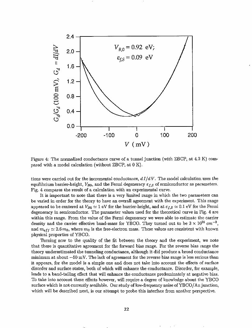
Figure 4 The normalized conductance curve of a tunnel junction (with ZBCP, at 4.2 K) com-pared with a model calculation (without ZBC!P, at O K).

tions were carried out for the incremental conductance, d 1/d V. The model calculation uses theequilibrium barrier-height, V~o, and the Fermi degeneracy Cf,s of semiconductor as parameters.Fig. 4 compares the result of a calculation with an experimental curve.

It is important to note that there is a very limited range in which the two pararneters canbe varied in order for the theory to have an overall agreement with the experiment. This rangeappeared to be centered at V~o = 1 eV for the barrier-height, and at Cf,s R 0.1 eV for the Fermidegeneracy in semiconductor. The parameter values used for the theoretical curve in l?ig. 4 arewithin this range. From the value of the Fermi degeneracy we were able to estimate the carrierdensity and the carrier effective band-mass for YBCO. They turned out to be 3 x 1021cm–3,and me~~ R 2.6 m., where m. is the free-electron mass. These values are consistent with knownphysical properties of YBCO.

Turning now to the quality of the fit between the theory and the experiment, we notethat there is quantitative agreement for the forward bias range. For the reverse bias range thetheory underestimated the tunneling conductance, although it did produce a broad conductanceminimum at about —50 mV. The lack of agreement for the reverse bias range is less serious thanit appears, for the model is a simple one and does not take into account the effects of surfacedisorder and surface states, both of which will enhance the conductance. Disorder, for example,leads to a band-tailing effect that will enhance the conductance predominately at negative bias.To take into account these effects however, will require a degree of knowledge about the YBCOsurface which is not currently available. Our study of low-frequency noise of YBCO/Au junction,which will be described next, is our attempt to probe this interface fi-om another perspective.

22

n

W!?w

-lo

-12

-14

-16

-18

I “J.“. 1-’*,

I a = 1.13

.-,

h T=77 K

I \ 1.==0.5 mA

-“t .\\ ::5%

-14

-:1

\LorentzianFunction

-16

012345

Log (f [Hz])

012345

Log (f [Hz])

Figure 5: Noise-power-density spectra of a junction for several bias levels.

RESULTS OF LOW-FREQUENCY NOISE STUDY

We see in Fig. 2 that there is considerable conductance noise in our small-area junctions,especially at high bias voltages. The conductance noise has also been observed in many otherjunctions with areas of 64 pm2 or larger. Thus these YBCO/Au junctions generally have substan-tial low-frequency resistance noise. To study junction noise behavior both horn a technologicaland a basic physics point of view, we developed a low-frequency noise measurement system.Technical details of our system have been given in a previous publication [8]. Here we showsome important results.

Fig. 5 shows the noise-power-density (NPD) spectra for a junction at room-temperature(left panel) and at 77 K (right panel). The room-temperature voltage noise power densityhas the usual l/~ frequency dependency, with a simple power-law dependence on bias current:Sv (f) m ~, as indicated by the 20 dB increase in Sv (~) for a ten times increase in bias current.This result allows a simple estimate of the normahked resistance fluctuation in a unit bandwidth.At 10 Hz, this figure is 6R/R = 6 x 10–4 /m. Moreover, this figure can be used to estimateresistance noise at any frequencies and for any given bandwidth. It thus offers an enormouspractical advantage for engineering high-TC superconductors electronic devices.

The NPD spectra at 77 K are more complicated. As indicated in the right half of Fig. 5,for small bias they resemble closely a Lorentzian function, which is frequency independent upto a characteristic frequency, beyond which the power-density rolls off as 1/~2. A Lorentzianspectrum indicates two-level-fluctuators (TLF), which switch between two quasi-stable levels inan energy space. Rogers and Buhrman [9] showed how small tunnel junction noise behavior canbe understood in terms of these TLF’s, acting either independently or with interactions betweenthem.

A clearer demonstration of TLF in our junctions is given in Fig. 6, taken at 4.2 K for a

23

> .5~050 100 150 200

f ( msec )n‘s -11~ -12 -~\& -13 - -cti = 2.4 (ins)ms -14 -

g -15 1 I I I

o 01 2 34

Log [f (Hz) 1

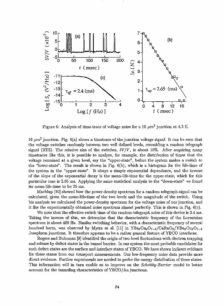
Figure 6: Analysis of time-trace of voltage noise for a 16 pm2 junction at 4.2 K

16 pm2 junction. Fig. 6(a) shows a timetrace of the junction voltage signal. It can be seen thatthe voltage switches randomly between two well defined levels, resembling a random telegraphsignal (RTS). The relative size of the switches, W/V, is about 107o. After acquiriag manytimetraces like this, it is possible to analyze, for example, the distribution of times that thevoltage remained at a given level, say the “upper-state’), before the system makes a switch tothe “lower-state”. The result is shown in Fig. 6(b), which is a histogram for the life-time ofthe system in the “upper-state”. It obeys a simple exponential dependence, and the inverseof the slope of the exponential decay is the mean-life-time for the upper-state, which. for thisparticular case is 2.65 ms. Applying the same statistical analysis to the “down-state” we foundits mean-life-time to be 25 ms.

Machlup [10] showed how the power-density spectrum for a random-telegraph-signal can becalculated, given the mean-lif~time of the two levels and the magnitude of the switch. Usinghis analysis we calculated the power-density spectrum for the voltage noise of our junction, andit fits the experimentally obtained noise spectrum almost perfectly. This is shown in Fig. 6(c).

We note that the effective switch time of the random-telegraph noise of this device is 2.4 ms.Takkg the inverse of this, we determine that the characteristic fkequency of the Lcmentzianspectrum is about 400 Hz. Similar switching behavior, with a characteristic frequency c~fseveralhundred hertz, was observed by Myers et al. [11] in YBa2Cu307_a/CaRu03 /YBa2Cu307_~Josephson junctions. It therefore appears to be a rather general feature of YBCO interfaces.

Rogers and Buhrman [9] identified the origin of two-level fluctuations with electron trappingand release by defect states in the tunnel barrier. In our system the most probable candidates forsuch defect states are the surface and interface states of YBCO. We have shown indirect evidencefor these states horn our transport measurements. Our low-frequency noise data provide moredirect evidence. Further experiments are needed to probe the energy distribution of these states.This information will in turn enable us to improve on the Schottky-.l?amier model to betteraccount for the tunneling characteristics of YBCO /Au junctions.

04 8 12 16f ( msec )

24

ACKNOWLEDGMENT

We gratefully acknowledge the support by the Department of Energy under Grant No.DEIA03-94ER14420.

References

[1] Yizi Xu, J. W. Ekin, C. C. Clickner, and R. L. Fiske. Oxygen annealing of YBCO/Gold thin-film contacts. In U. Balu Balachandran et al., editors, Advances in Cryogenic EngineeringMaterials, volume 44, Part B, pages 381–388, New York, 1998. Plenum Press.

[2] Chia-Ren Hu. Midgap surface states as a novel signature for d--wave superconductivity.Phys. Rev. Lett., 72(10):1526, 1994.

[3] J. W. Ekin et al. Correlation between d-wave paring behavior and magnetic-filed-dependentzero-bias conductance peak. Phys. Rev. 13,56:13746, 1997.

[4] M. Covington et al. Observation of surface-induced broken time reversal symmetry inYBa2Cu307 tunnel junctions, F%ys. Rev. Lett., 79(2):277, 1997.

[5] M. Fogelstrom, D. Rainer, and J. A. Sauls. Tunneling into current-carrying surface statesof high-TC superconductors. Phys. Rev. Lett., 79(2):281, 1997.

[6] J. M. Vanes, Jr. et al. Electron tunneling into single crystal of YBa2Cu307-J. Phys. Rev.B, 44:11986, 1991.

[7] J. W. Conley and G. D. Mahan. Tunneling spectroscopy in GaAs. Physical Review,161(3):681, 1967.

[8] Yizi Xu, J. W. Ekin, and C. C. Clickner. Low-frequency noise in YBCO/Au junctions.In IEEE Trans. Appl. Supercond., 1999. Proceedings of 1998 Applied SuperconductivityConference, Palm Springs, California, 1998.

[9] C. T. Rogers and R. A. Buhrman. Composition of l/~ noise in metal-insulator-metal tunneljunctions. Phys. Rev. Lett., 53(13):1272, 1984.

[10] Stefan Machlup. Noise in semiconductor: Spectrum of a tw~parameter random signal. J.Appi. Phys., 25:341, 1954.

[11] K. E. Myers, K. Char, M. S. Colclough, and T. H. Geballe. Noise characteristics ofYB%CusOT_6/CaRuOs/YBazCu307_~ Josephson junctions. Appi. Phys. Lett., 64(6):788-790, 1994.

25

AN EFFICIENT NEAR-FIELD MICROSCOPE FOR THERMAL MEASUREMENTS

G. S. Kino, D. A. Fletcher, K. B. Crozier, K. E. Goodson, and C. F. Quate

Ginzton Laboratory, 450 Via Palou, Stanford University, Stanford CA 94305-4085Tel: 650-723-0205, Fax: 650-725-2533, EM: [email protected]

ABSTR4CT

We describe the application of the solid immersion lens (SIL) to scanning near-field infrared microscopy. The advantage of the SIL over other near-field approachesis its high efficiency. With the use of micromachined silicon lenses of a few micrcmsdiameter, a spot size of 1 pm can be obtained at 5 Urn wavelength. The microscopewill be used to measure the temperature of interconnects in integrated circuits, whichare being excited by high speed pulses and for infrared spectroscopy of small samp”lessuch as Ga4s laser diodes.

INTRODUCTION

This paper is a progress report on the development of a new technique for infrared measurementsof temperature distribution and the emission spectrum with high spatial definition of small scalesemiconductor devices with feature sizes as small as 100 nm. Since standard microscopes are sodifficult to make in the far infrared range and their definitions are inadequate for modem require-ments, we are proposing a different approach, scanning optical microscopy using microscopic sizedlenses, called Solid Immersion Lenses (SIL), a few microns in diameter mounted on cantilevers.These lenses, made by conventional methods in the millimeter size range, were invented a.tStanfordby Kino and his coworkers, l’2’3and are now being investigated for use in high density optical storageby a number of manufacture such as TeraStor in this country and Sony and Nikon in Japan. It is ourintention to use SILS for efficient near-field imaging to obtain focused spot sizes well below thenormal diffraction limits of standard microscopy.

We use micromachining techniques to manufacture these microscopic sized lenses. This tech-nology is inexpensive and with it devices can be made and reproduced in large quantities. This methodof manufacturing and assembling optical microscope components gets us away from the conventional19th century approach of lapping and grinding lenses, and then assembling them by hand. At thesame time the SIL yields better definitions than were heretofore available and, because of the smalllenses employed, the possibility of being able to place the tip of the lens extremely close (100 nm)to the sample being measure~ with low chromatic and spherical aberration and relatively uncriticallens design.

PRINCIPLE OF OPERATION OF THE SOLID IMMERSION LENS

It is extremely difficult to make even a standard infrared microscope. The objective lenses arenot easily available and must be made of unusual materials such as germanium and silicon, and in therare instances when they can be obtained are extremely expensive. The spot size, defined as thedistance between half power points of the focused beam in an optical microscope, optical storage sys-tem or lithography system is determined by difllaction to be approximately 1./(2lL4), where k is the

26

flee space wavelength, and lL4 is the numerical aperture of the objective lens defined by the relationAU= n sinOO,where 60 is the maximum ray angle to the axis. For an inflared microscope with L= 5~m andNA = 0.7, the spot size defined this way is 3.6 pm.

One approach for improving the definition is to employ near-field optics in the manner describedby Betzig.4 In his near-field scanning optical microscope (NSOM), he used a tapered optical fibercovered with a metal film with a small pinhole at the end. The definition of the system is determinedby the size of the pinhole rather than by diffraction, and can be 50 nm or less. The advantages of thesystem are its excellent definition and its polarization preserving capability. A major disadvantage ofthis approach is its poor light efficiency with 30 to 50 dBs of transmission loss.

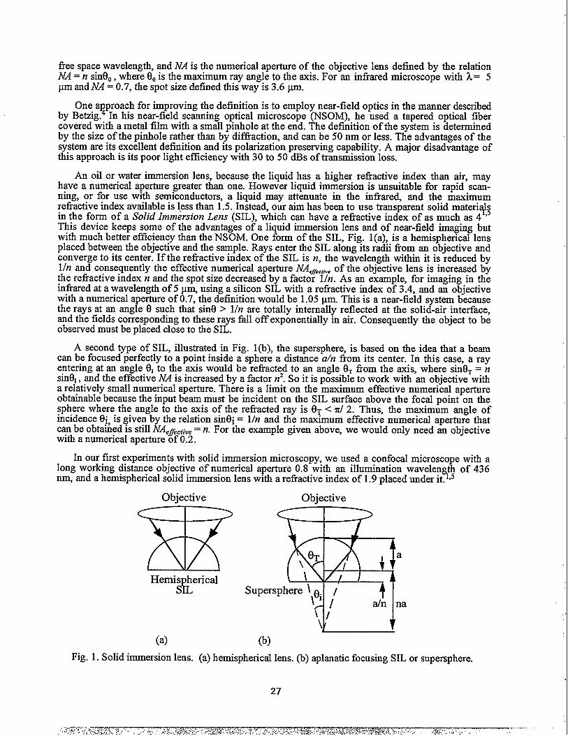
An oil or water immersion lens, because the liquid has a higher refractive index than air, mayhave a numerical aperture greater than one. However liquid immersion is unsuitable for rapid scan-ning, or for use with semiconductors, a liquid may attenuate in the infkre~ and the maximumrefractive index available is less than 1.5. Instead, our aim has been to use transparent solid materi~~in the form of a Solid Immersion Lens (SIL), which can have a refractive index of as much as 4 ‘This device keeps some of the advantages of a liquid immersion lens and of near-field imaging butwith much better efficiency than the NSOM. One form of the SIL, Fig. 1(a), is a hemispherical lensplaced between the objective and the sample. Rays enter the SIL along its radii from an objective andconverge to its center. If the refractive index of the SIL is n, the wavelength within it is reduced byl/n and consequently the effective numerical aperture NA,fi.c,iv.of the objective lens is increased bythe refractive index n and the spot size decreased by a factor l/n. As an example, for imaging in theinfrared at a wavelength of 5 pm using a silicon SIL with a reflective index of 3.4, and an objectivewith a numerical apertureof 0.7, the definition would be 1.05 pm. This is a near-field system becausethe rays at an angle 0 such that sine > l/n are totally internally reflected at the solid-air interface,and the fields corresponding to these rays fidl off exponentially in air. Consequently the object to beobserved must be placed close to the SIL.

A second type of SIL, illustrated in Fig. l(b), the supersphere, is based on the idea that a beamcan be focused perfectly to a point inside a sphere a distance ah from its center. In this case, a rayentering at an angle EIIto the axis would be refracted to an angle e= from the axis, where sin6~ = nsinei, and the effective NA is increased by a factor n2. So it is possible to work with an objective witha relatively small numerical aperture. There is a limit on the maximum effective numerical apertureobtainable because the input beam must be incident on the SIL surface above the focal point on thesphere where the angle to the axis of the refracted ray is eT < d 2. Thus, the maximum angle ofincidence Eli,is given by the relation sin(3i= I/n and the maximum effective numerical aperture thatC* be obtained is stall~~e~ec~ive= n. For the example given above, we would only need an objectivewith a numencal aperture of 0.2.

In our first experiments with solid immersion microscopy, we used a confocal microscope with along working distance objective of numerical aperture 0.8 with an illumination wavelen th of 436

.~5nm, and a hemispherical solid immersion lens with a refractive index of 1.9 placed under It. *

Fig.

Objective

xHemis herical

$ IL

Objective

a

Supersphere \e. /\’ / ah na

\,/ 1

(-b)(a)

. Solid immersion lens. (a) hemispherical lens. (b) aplanatic focusing SIL or supersphere.

27

The SIL had a NAefleC(iVeof 1.52 and was used to image various small structuresat a wavelength of436 nm. The smallest structures imaged were the 100 nm lines and spaces in photoresist shown inFig. 2. In comparison, the smallest structures that were observed with the confocal microscope, witha 0.9 N.A. objective under the same conditions were 150 nm lines and spaces with a calculatedminimum detectable periodicity of 242 nm (120 nm lines). The calculated minimum detectable peri-odicity for the SIL is 144 nm (72 nm lines).

30

25

.+208~ 15A

10

53000 3400 3800 4200 4600

Position (rim)ao

Fig. 2. Image and line scan of a 200 nm period grating.

lPi\! t , , # 1 ,

0.9

0.8

0.7

0.2

0.1

0

. . . . .

. . . . .

. . . . .

.

. .

. . . . .

. . . . .

. . . . . . . . . . . ... .

. . . . . . . . ... .

7..........Re@ve

.Wwgr. . . . . .1:

. . .0.8i

-0.68... . ..-

0.55. . . . . . . . . .

-J0.35

. .

. ... .

. . .

. ... .

. ... .

. . . . . . . . . . . .

0 0.5 1 15 2 2.5 3 3.5r ~m]

Fig. 3. Point spread functions for normalized intensity with different air gaps.

One question that arises with the use of an SIL is the effect of an air gap between the SIL and theimage plane on the point spread function (PSF) and the transmission efficiency. Codes based onvector field theories have been developed for determining the fields outside the lens in air and inmultiple layer systems such as that of an optical disk or photoresist on silicon@ The conclusion ofthese computations is that in the optical range, with SILS with a refractive index of 2 or so, thetransverse resolution between half power points, d, is given ftily accurately by the simple formulad= )J2NAeff where NA=

J= n sin e. n is the refractive index of the SIL and 00 is the maximum ray

angle from the axis WI in the lens, provided that the air gap is kept to less than 100 nm at a wavelength of 0.7 pm. For higher refi-active index materials or shorter wavelengths, the air gap must bestill thinner. Calculations for the point spread fiction (PSF) at a silicon substrate for a silicon SIL

28

with a refractive index of 3.4, working at a wavelength of 5 pm are shown in Fig. 3. It will be seenthat the spot size between the half power points is 0.98 ym with no air gap. But as the air gap is in-creased the spot size increases by 10°A with an air gap of 0.2 pm and the intensity on axis drops to48% and total power to 68% at this point. If the SIL were used as a receiver of thermal radiation, theefficiency would again be 68?40with an air gap of 0.2 pm. This efficiency is far higher than that ofthe NSOM.

We are also concerned with the tolerance for manufacturing these lenses. An image formed bythe input beam may be shown to be demagnified in the hemispherical SIL by a factor l/n in both theradial and axial directions. The hemispherical SIL is extremely tolerant. By examining when theaberrations due to field curvature become large enough to cause a phase error of 7r/2 between theouter and inner rays of a focused be% we find that the field of view of the hemispherical SIL, Admis given by the relation2’5 ,

Ad= =J

Zlk

n(n - 1)sin2(30‘(1)

where a is the radius of the hemisphere. For k= 436 nm, n = 2, Sintlo= 0.8, a = 1 mm, we find thatAdm = 39 pm. This is a relatively large field of view, and is the reason why the image in Fig. 2 ex-tends over a relatively large region without appearing to be aberrated.

The tolerance in the axial direction is also broad, If the thickness of the hemisphere is changed,the input beam may be refocused to focus on the flat surface provided that the lens thickness variesby less than Az-, where

‘~=E*(2)

For a supersphere, it can be shown that to first order in r, the radial demagnification is llnz andthe field of view is comparable to that of the hemispherical lens. The demagnification in the zdirection is l/n3 However there is a fust order error in the length tolerance, % which can beshown to be given by the approximate formula

Az.=~+722–1 2sm 60’(3)

where 60 is the maximum ray angle inside the lens. Using the same parameters as for the hemispheri-cal SIL, we find that is 0.3 pm. Thus, the tolerance on the length of a supersphere, of typically 1 to 3mm diametersis very tight although, for n = 2, the tolerance on the axial position of the objective iseight time (n ) this value. However for silicon, at a wavelength k = 5 yq with n = 3.4, and sin60 =0.8, this simple formula gives a tolerance in the position of the objective of 49 pm and a length tol-erance of 1.25 pm. The reason for the large tolerance is that with a high refractive index, incidentrays from air are bent towards the focus and their initial direction becomes relatively uncritical.

SCANNING TECHNIQUES

Although it is possible to obtain a large field of view with an SIL, this is not easy to do in practicebecause it is difficult to keep the flat surface of the SIL close enough over a large area to the objectbeing observe. In our early experiments, we ground off the hemisphere to a conical shape so that thebottom surface would be of the order of 100 pm in diameter. In optical storage the SIL isincorporated into a floating head so that it floats on an air bearing over a rotating disk. But to ob-serve substrateswhich are not flat, these stratagemsare not good enough.

Recently Ghislain and Elings7’8have built a different type of near-field microscope using a solidimmersion lens. The SIL, as shown in Fig. 4, was tapered at its lower end to a cone half angle of 65°,and a supersphere was used with a material of refractive index 2.2 at a wavelength of 442 nm, and anapodized beam with an M4e~ect~ve of 2, yielding a theoretical spot size of 120 nm. The SIL was

29

mounted on a soil cantilever in a force microscope structure (Fig. 5) so that its distance from thesample could be controlled. The tip of the SIL was less than 1 pm diameter, which made it possible toobtain very small spacing between the tip and the sample. The sample was scanned to form a com-plete image in the same way as with a near-field scanning optical microscope (NSOIVQ.Images weretaken of metal films laid down on glass with periodically spaced holes in them. Optical contrast wasobtained with a definition of the order of 150 nm. Other features with a definition of the order of 70nm were observed. This phenomenon was thought to be due to topography effects associated withthe exponential fall off of fields away from the tip. Cooperating with us at Stanford, they also carriedout photolithography with this same system and obtained good results.s

It is our intention to make SILS only a few microns diameter and use micromachining techniquesto manufacture them. This eliminates the need for a long working distance objective. The SILS willbe mounted on small cantilevers with a rapid response time in the same manner as with scanningforce microscopy. In that case the supersphere and even aspherical lenses would become more usefid,for now the tolerance of the objective lens position and focusing would be very large. Furthermore,with such small lenses the shape of the lens becomes much less critical, for now errors in phase donot accumulate over a long distance, and so aberrations are fm smaller. In addition, by changing thechemical etching conditions there is the possibility of making aspheres so that the input beam couldbe rectilinem, i.e., we would not need a high power objective lens. We have calculated in some detailthe nature of such aspherical lenses which, typically, are elliptical in shape.

Objective

‘e’!Optical axis

@

Critical angle

Outer

}\ 1’

+1

rays

Fig. 4. SIL microscope structure.7’8 Fig. 5. SIL mounted on a cantilever.7>8

As an example of the advantages of using microlenses for eliminating aberrations, we havecalculated with the optical design program ZEMAX the point spread function (PSF) of an imper~cthemispherical lens. We took the lens to be a hemisphere of radius a minus a parabol~ r‘= 0.04z . .The calculated PSFS for ~o values of the hemisphere radius a, 3.5 pm, and 3.5 VU with k = 325 nmand n = 2, are shown in Fig. 6. It will be seen thatthe PSF of the smallest lens has very low sidelobes,but as the radius of the hemisphere is increased, the sidelobes get worse. With the largest lens, the ef-fect of the nonsphericity is to ruin the PSF. Furthermore, we observe that even though the lens isnonspherical, aberrations are negligible. We conclude that the requirement for a perfecr sphericalshape becomes less critical as the lens size is reduced to the microscopic dimensions proposed here.

In previous applications, SILS have been sh~ed with traditional lens-making techniques that aretime consuming, labor intensive, and expensive. ‘ Microfabrication would enable hundreds of SILS assmall as 5 pm to be fabricated using standard lithographic tools; the smallest SILS manufactured withmechanical grinding techniques are about 1 mm diameter. An SIL fabricated on the end of an AFMcould be scanned above the surface of a sample held within its near field, concentrating light on orcollecting light from the sample. Such a device could be used for collecting near-infrared wavelengthstransmitted through a cell or thermal radiation from a self-heated interconnect. A major advantageof the use of this type of technology is that the micromachined tip the SIL will also be used as a

30

Scanning Force Microscope (SFM). This makes it possible to adjust the tip-sample spacing and tomake independent measurements of the sample profile.

1.0a =3.5 pm 1.0 a =3.5 mm

0.8a

a) 0.8-0~ 0.6 ~ 0.6

—E! e~ 0.4 < 0.4<

0.2 0.20 0

-3.13 pm o 3.13pm -3.13pm o 3.13pmRadius r Radius r

Fig. 6. The PSFS for two different sizes of nonspherical lenses.

FABRICATION OF AN INTEGRATED CANTILEVER AND MICROLENS

Our objective is to demonstrate the optical resolution of an integrated SIL and SFM at infhredwavelengths. Single crystal silicon has been chosen as the lens and cantilever material due to theavailability of Si processing techniques and equipment, the proven use of Si cantilevers in scanningprobe systems, and the high index of Si at the infrared wavelengths important to spectroscopy,thermometry, and other applications. Scaled down versions of the device illustrated in Figs. 3 and 4are being fabricated with microlens diameters ranging from 5 to 15 pm and cantilevers from 50 to200 pm long. In order to localize the region of contact between the sample and the SIL, a tip isformed on the opposite side of the lens. A conical tip with radius of curvature less than 1 P andsides angled at 60 degrees from the vertical provides sufficient localization without blocking high-angle rays. Such a tip is much larger than the typical NSOM tip and allows easy alignment of the fo-cal point, but it is small enough to allow a very close approach to a rough surface. Because of its rel-atively large size, it is also not subject to the same wear as an NSOM tip, as has been shown experi-mentally by Ghislain et al.TJSThough many techniques for fabricating sharp, high aspect-ratio tipsexist, methods for less-sharp, low aspect-ratio tips with large side angles must be developed.

Fabrication of the integrated SIL cantilever presents two primary processing challenges: (1)formation of the lens shape and (2) double-side processing of a thin film to create a tip opposite thelens. Arrays of microfabricated lenses are used with focal plane array detectors and wave-front sen-sors, among other devices. The method chosen for use in this work is based on reflow of photoresistpillars and transfer of the shape into a substrate by dry etching9. This approach uses standard pho-tolithography to define the diameter of the lens but requires a non-standard dry etch to consume thelens material and photoresist mask at the same rate. A fabrication process (Fig. 7) has been designedto create a xnicrolens and tip on opposite sides of a thin Si cantilever. Pillars are formed in photore-sist and reflowed thermally or in acetone vapor to form a three-dimensional etch mask for the lens.The SIL is formed by reactive ion etching (REI) the top Si of a Simox SOI wafer that has had anadditional 15 pm of Si grown epitaxially. The selectivity (Si : photoresist) of the etch process and thereflow conditions are used to control the shape of the lens. A thin film of thermal oxide is grown toform an etch stop for the cantilever release. The SOI with SILS is then anodically bonded to a Pyrexwafer with pits etched to protect the lens. The bottom Si and middle oxide of the SOI wafer isremoved in TMAH and HF, respectively, leaving the thin top Si layer in which the lens tip and can-tilever will be formed. Tips are then formed using reflowed photoresist and RIE opposite the lens.Next, cantilevers are masked and etched into the remaining top Si with RIE, stopping on the thermaloxide previously grown on the lenses. Finally, the thermal oxide is removed with HF and the can-tilevers held by the support wafer are released by backside etching or wafer sawing. Note that thisprocess could be used to create lenses and cantilevers in other materials.

1. Definepillamin photoresistom an SOI wafer

5. Patternprotectivepits in a

2. Reflowthe photoresist 3. Transferthe curvedshapethermallyor in acetone onto Si with RIEvaporto forma curvedshape

~~

7.Anodicallvbondthe classwaferto&e SOI waf;r

mmm

9. Definethe lens tip in 10. Etchthe tip with RIE 11.Definethe canileverinphotoresist photoresist

photoresist H mI I silicon Dn

3.

4. Growthermaloxideon lenssurfaceto serveas an etchstop for backsideprocessing

Removethe thermaloxide.bulkSi,andburiedoxidetoexposetheback side of the lens

12..Etch the cantileve~with RIEusingthermaloxideas anetch stop

oxide

Pyrex

13. Removethe thermaloxidefromthe cantileverandlenswithanHFdip and release thethe die with a wafersaw

Fig. 7. Steps in the micromachining of the SIL and tip mounted on a cantilever.

The lens fabrication and cantilever fabrication processes will be joined to make an intematedcantilever and SIL. A critical step in the process is afignment of the tip ‘md distance from the l&s tothe tip apex. A high-resolution mask aligner will be used for alignment, and thin-film thickness mea-surements during etching will control thickness.

We expect to be testing our first infrared SILS mounted on cantilevers within the next fewmonths and then to go on to test them first for imaging simple structures and later for measurementof pulsed thermal sources such as interconnects in high speed circuits.

Hemispherical SILS and short focal-length microlenses have been fabricated in single cx-@al Si. Aphotoresist reflow method using acetone vapor has been developed, and a plasma etch recipe hasbeen refined to transfer and extrude the photoresist lens shape into Si (Fig. 8). Si cantilew:rs bondedto Pyrex have been released (Fig. 9). A process for fabricating the Si cantilevers which enableslithography on both sides of the top Si of an SOI has been created.

32

Fig. 8. Microlens in Si. Fig. 9 {eleased Si cantilevers bonded to Pyrex.

ACKNOWLEDGMENTS

The infrared portion of this work was supported by the Department of Energy and the StanfordNanofabrication Facility. We would like to thank Tom Hunt for the calculations given in Fig. 6.

1.

2.

3.

4.

5.

6.

7.

8.

9.

FOOTNOTES

S. M. Mansfield and G. S. Kino, “Solid Immersion Microscope,” Appl. Phys. Lett. 57, 2615-2616(1990).

S. M. Mansfiel& W. R. Studenmun& G. S. Kino, and K. Osato, “High Numerical Aperture LensSystem for Optical Storage,” Opt. Lett. 18,305-307 (1993).

I. Ichimur~ S. Hayashi, and G. S. Kino, “High Density Optical Recording Using a SolidImmersion Lens,” Appl. Opt., 36, 4339-4348, (1997).

E. Betzig, J. K. Trautman, R. Wolfe, E. M. Gyorgy, P. L. Finn, M, H. Kryder and C. H. Chang,“Near-Field Magneto-Optics and High Density Data Storage,” Appl. Phys. Lett. 61, 142 (1992).

S. M. Mansfiel& “Solid Immersion Microscopy,” Ph.D. Dissertation, Department of AppliedPhysics, Ginzton Laboratory, Stanford University (March 1992).

M. Mansuripur, “Effects of High-Numerical-Aperture Focusing on the State of Polarization inOptical and Magneto-Optic Data Storage Systems,” Appl. Opt. 30, 3154-3162, (1991).

L. P. Ghislain and V. B. Elings, “Near-Field Scanning Solid Immersion Microscopefl Appl. Phys.Lett. 72,2779-81 (1998).

L. P. Ghislain, V. B. Elings, K. B. Crozier, S. R. Manalis, S. C. Minne, K. Wilder, G. S. Kino, andC. F. Quate “Near-Field Photolithography With a Solid Immersion Lens,” Appl. Phys. Lett. 74501 (1999).

T. Serikawa and S. Shirai, “Modelling of Lift-Off Sputter Deposition and Application toFabrication of a Microlens,” Thin Solid Films, 281-282,246-248 (1996).

33

ELECTROMECHANICAL FRACTURE IN PIEZOELECTRIC CERAMICS

Huajian Gao and David M. Barnett

Division of Mechanics and ComputationStanford University

Stanford, CA 94305, U.S.A.

ABSTRACT

The reliable operation of smart devices and structures depends on the integrity ofthe materials chosen for sensor and actuator components. We investigate the crack-ing behavior of piezoelectric ceramics, brittle materials whose nonlinear response isdominated by electrical effects. We simulate these microstructural effects using dis-crete electric dipoles, and find that the crack driving force at the local length sca’le isexpressed solely in terms of mechanical opening stresses. The resulting predictionsof failure under combined electromechanical loading conditions agree qualitativelywith empirical observations. An investigation of permeable surface conditions re-veals that the effect of air inside an open crack is negligible except in the case of analmost perfectly sharp crack.

INTRODUCTION

The growing demand for smart systems and structures raises concerns about the mechanicalintegrity of the materials used for sensor and actuator components. In this study we attemptto resolve some basic discrepancies between theoretical predictions and empirical observations ofthe cracking behavior of piezoelectric ceramics, some of the most widely used transducer materials.Numerous experimental studies have been performed on specimens of lead zirconate titanate (PZT)with cracks perpendicular to the poling axis, loaded by tension and electric field along the axis. Incompact tension, three-point bending, and Vickers indentation tests, researchers have found thatthe application of electric field aligned with the material poling direction promotes cracking, whilethe opposite sense of the field inhibits cracking [1, 2]. However, the natural extension of linearelastic fracture mechanics to. account for electrical contributions to the energy balance predictsthat the field should inhibit fracture irrespective of its sign [3, 4, 5].

Some attempts have been made to explain the empirical results in terms of the permeability ofthe crack interior and the resulting change in boundary conditions once the crack opens [6, 7, 8].But we show that the inhomogeneous crack-face conditions cannot alter the essential characterof the relationship between applied field and critical stress. Further, if the medium that fills thecrack is air, it plays a negligible role except in the case of extremely slender initial voids. A more

34

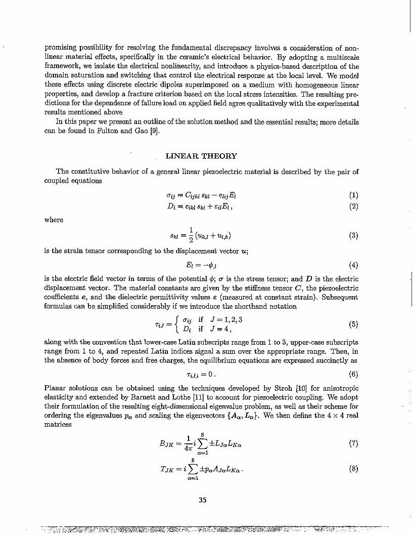
promising possibility for resolving the fundamental discrepancy involves a consideration of non-linear material effects, specifically in the ceramic’s electrical behavior. By adopting a multiscaleframework, we isolate the electrical nonlinearity, and introduce a physics-based description of thedomain saturation and switching that control the electrical response at the local level. We modelthese effects using discrete electric dipoles superimposed on a medium with homogeneous linearproperties, and develop a fracture criterion based on the local stress intensities. The resulting pre-dictions for the dependence of failure load on applied field agree qualitatively with the experimentalresults mentioned above

In this paper we present an outline of the solution method and the essential results; more detailscan be found in Fulton and Gao [9].

LINEAR THEORY

The constitutive behavior of a general linear piezoelectric material is described by the pair ofcoupled equations

where

sk~= : (~k,l + ?@) (3)

is the strain tensor corresponding to the displacement vector u;

El = –4,1 (4)

is the electric field vector in terms of the potential ~; ~ is the stress tensor; and D is the electricdisplacement vector. The material constants are given by the stiffness tensor C, the piezoelectriccoefficients e, and the dielectric permittivity values .s (measured at constant strain). Subsequentformulas can be simplified considerably if we introduce the shorthand notation

{

Oij if J= 1,2,3TiJ =

Di if J=4,(5)

along with the convention that lower-case Latin subscripts range from 1 to 3, upper-case subscriptsrange from 1 to 4, and repeated Latin indices signal a sum over the appropriate range. Then, inthe absence of body forces and free charges, the equilibrium equations are expressed succinctly as

TiJ,i = O . (6)

Planar solutions can be obtained using the techniques developed by Stroh [10] for anisotropicelasticity and extended by Barnett and Lothe [11] to account for piezoelectric coupling. We adopttheir formulation of the resulting eight-dimensional eigenvalue problem, as well as their scheme forordering the eigenvalues pa and scaling the eigenvectors {Aa, I&}. We then define the 4 x 4 realmatrices

813JK= &i ~ %LJaLKa (7)

a=l8

TJK ==i ~ &pnAJaLKo . (8)a=l

35

The problem of an insulated crack in a linear piezoelectric has been studied extensively [3, 5, 12],and its solution is well known. For a crack in the (ZI, xz)-plane, bounded by IZl ] < a, the boundaryconditions can be written succinctly as

7z~(zl,0) = O, Izll < a. (9)

The four intensity factors are derived from

KJ = ;RO ~m72J(z), (lo)

in terms of the remote loading Ti~. The energy release rate then takes the compact form

Glinear = ~KJB~~KL (11)

(12)

These formulas apply to cracks at arbitrary orientations in general linear piezoelectric materialsunder any combination of remote loads. However, they cannot explain experimental observations,even for the relatively simple case of a crack perpendicular to the poling of a transversely isotropicsample, subjected to Mode I stress and electric field along the poling axis. As menticmed at theoutset, estimates of the failure load obtained from (11) or (12) show an even functional dependenceon applied field, while empirical data suggest an odd dependence. The remainder of the paper isdevoted to finding a resolution to this contradiction.

PERMEABLE BOUNDARY CONDITION

The analysis of the previous section depends on the idealized approximation that the cracksurfaces remain perfectly insulated during loading. However, in many experiments and in almostall practical applications, upon opening the crack interior fills with an electrically permeable fluid,usually air. It has been suggested [7, 8] that the resulting inhomogeneous boundary condition playsa significant role in the fracture of piezoceramics. We now examine the effects of treati:ng the fluidinside the crack realistically, as an isotropic dielectric with no stiffness.

When a slit crack opens into an elliptical profile, the deformed medium can be t rested as abimaterial inclusion problem. For elastic bodies subjected to uniform far-field stresses, Eshelby [13]showed that the strain inside an ellipsoidal inclusion is a constant. Deeg [14] generalized the methodto apply it to piezoelectric materials, where the applied fields include electric displacements aswell as tractions. He showed that the fields induced in an ellipsoidal piezoelectric inhornogeneity,both strains and electric field, are constant under any uniform remote loading conditions. As aparticular case of Deeg’s result, we can take the inclusion to be a dielectric material, with no stiffnessor piezoelectric coupling. In short, we conclude that, when uniform electromechanical loads areapplied to a cracked piezoelectric solid, the fluid that fills the crack has a constant electric field ~.

Now, in the absence of free charge on the crack surfaces, the electric displacement ncmmalto theinterface must be continuous. Within the constraints of infinitesimal deformation theclry, the fluxon the solid side of the interface can be approximated by 724over virtually the entire crack length.Meanwhile, the flux in the fluid is equal to the constant value ~~2, where ~ is the PermittivitYof the medium that fills the crack. The continuity of the electric displacement, together with thetraction-free conditions on the crack surfaces, can be expressed as

T21(ZI, O) = c$~4FE2, IZII < a. (13)

36

But we can also relate the electric field within the crack to the voltage difference across the fluidand the crack-opening displacement:

These conditions are sufficient to solve for the fields throughout the bimaterial.Because the fluid stores electrostatic energy, an overall energy balance must be performed to

determine the portion of the work done on the specimen boundary available to drive the crack.The work that is stored in the solid is given by the piezoelectric enthalpy WsOl, and that stored inthe fluid is the electrostatic energy U*. With the presumption of fixed grips (dA = O) and fixedvoltage (W = O)at the boundary, the crack driving force consists of contributions from both media

G= GsO1+G*, (15)

where

()@=_~ >A,V

(16)

and dA is an increment of crack area.Using the definition (10), we find the intensity factors for the permeable crack,

KJ = (7~~ – ii~4EEz)@, (17)

and we can express the solid’s contribution to the energy release rate as

GSO1_– &KJBy~KL.

Substituting expressions for the crack-opening displacements

(18)

into (14) yields

The method can be applied to arbitrary loadlng situations, but in many problems of interest thereis enough symmetry so that fil = O. In this case the fluid’s contribution to the crack driving forcetakes the form

2 ZJ (7H - ~J4~~2) ,Gfl – :g@@

and the total energy is given by (15), (18), and (20).

ELECTRICAL NONLINEARITY

The class of piezoceramic materials we are interested in typically

(20)

.

displays extremely brittlemechanical response with almost no plasticity. The electrical behavior, on the other hand, ex-hibits significant nonlinear characteristics, most notably the hysteresis associated with polarizationswitching. In fact, it can be shown that the region of electrical nonlinearity around a crack tip ina piezoceramic dwarfs the mechanical nonlinear zone. It is reasonable, therefore, to separate thelength scales at which electrical and mechanical nonlinear effects play a role. In this section we

X2

t

xl

Figure 1: Crack Interacting with a Discrete Dipole.

focus on an intermediate length scale, at which the stress fields appear to follow linea,r constitu-tive laws, while the electric field exhibits nonlinearity. In this framework, we develop a model forelectrical nonlinearity based on the switching behavior of polar domains in ferroelectrics.

When a uniform low-level electric field is applied to a piezoelectric solid, the internal polarizationappears to respond in a linear homogeneous fashion. But this macroscopic behavior is the aggregateeffect of a vast collection of randomly oriented ferroelectric domains. Upon closer inspection,these local inhomogeneities gain significance and, as the electric field is intensified, may dominatethe material response. We simulate the local complexity directly, using discrete electric dipolessuperimposed on a homogeneous medium with the macroscopic piezoelectric properties. Eachdipole represents the deviation of a given domain’s polarization vector fromby the linear constitutive law. Now, while a dipole @ in a uniform electricany variation in the field results in a net force:

F=(vE)@.

the response predictedfield is at equilibrium,

(21)

Because the region surrounding a crack tip is characterized by severe gradients in all the fieldquantities, the crack exerts a net force on dipoles representing the nearby polar domains. This non-local interaction implies that an energy density formulation cannot capture the type of nonlinearmaterial effects we are investigating; they can only be understood within the multiscale framework.

As a first approximation to the case of general nonlinearity around a crack tip, we e:camine theeffect of a single dipole in the plane of the crack, as shown in Fig. 1. It is meant as a simplifiedcharacterization of the net effect of the many dipoles needed to describe any deviations from linearbehavior. The influence of the dipole must then be sufficient to cancel the crack-tip singularityin the electric displacement; this condition fixes the dipole strength for a given position r. If aJ-integral were calculated for the contour labeled 17a,the result would be the linear estimate of thecrack driving force, given by (11). But the dipole represents the material microstructure, so thecontour rC must be used to capture the local driving force; the resulting J-integral corresponds to

38

a crack cleaving the microstructure. The difference between the “apparent” and local J-integralsis precisely the force exerted on the dipole by the crack.

For an insulated crack, the local energy release rate can be expressed in terms of the localintensity factors Kc as

(22)

If the cracked sample is transversely isotropic, and the loading is symmetric, the relationshipbetween local and apparent intensity factors is captured by

T4J .K;=K~– —Kd ,

T44(23)

where K? = T2~@. From the form of the energy release rate (22) it is immediately apparentthat the onset of fracture is determined solely by the local intensity factors K$. The fact that theelectrical intensity K: vanishes indicates that, at the local length scale, the crack extension is drivenby purely mechanical opening forces. In other words, the combination of electrical and mechanicalloads applied in the global view are experienced as “effective” mechanical intensities at the locallevel. These effective stresses can be interpreted in terms of the mismatch strains associated withlocal domain switching.

In the case of a fluid-filled crack, the solid’s contribution to the driving force is evaluated atthe local level, and is given by (22) and (23), with the apparent intensity factors for a permeablecrack (17). The contribution from the fluid, however, is dominated by the overall expansion of theelliptical cavity, so its treatment is accomplished completely at the global level. The effect can becalculated from (19) and (20).

The analysis of these problem reveals a remarkable feature the local energy release rate is infact independent of both the dipole’s position r and its strength ~. This invariance is particularlyvaluable because it allows us to sidestep the difficulties normally associated with characterizing thelocal electrical response of ferroelectrics. That is, although an understanding of the microstructureis vital to the development of our local model, the end results are independent of the specificmaterial details. What makes the theory powerful is that it takes account of the complicatednature of electrical nonlinearity without requiring any extra experimental measurements.

NUMERICAL EXAMPLE

To illustrate the analytical results presented above, we consider a specimen of PZT-4, a trans-versely isotropic piezoelectric ceramic whose material properties are given by Park and Sun [1]. Fora through crack with faces perpendicular to the poling direction loaded under remote tension amand electric field -E@ along the poling axis, the symmetry conditions necessary for (20) and (23) aresatisfied. By setting G equal to a critical toughness value, we can determine the failure stress crC~as a function of the applied field. This function is plotted in Fig. 2(a) for a linear material with acrack of half-length a = 1 mm and a critical stress at zero external field of 5 MPa. The insulatedcase (F= O) is shown together with the results for an air-filled crack (E= .50). The techniquesdescribed above can be extended to the case of a slender elliptical void. Figure 2(a) includes resultsfor air-filled voids with a range of initial aspect ratios p. (ratio of minor axis to major axis). It isevident that the energy release rate for a linear material is dominated by a term that is quadraticin Em, giving rise to the nearly even functions depicted in Fig. 2(a). The permeable boundarycondition weakens the electrical singularity, thereby reducing the effect of electric field on failure

39

t I {–0.5 –0.25 0.25 0.5

Em (l&/m)

(a) LinearMaterial

12.------- ECo

<’1

1

___ ~=&O, PO= 1/10010\

<% —-— F = &(),pi) = 1/1000‘<’\ — E=&l), po=o

8 .‘\\\

‘\. \\>.\

‘s \. ‘\.!LGg

Y~<>\

\.

86b4

“+ -\ --% t..x 1‘-------..L...A...A-..>.,\.. \-...\.. \

.......

k I–0.5 –0.25 ( 0.25 0.5

Figure 2: Failure Stress vs. Applied

-Em (MV/m)

(b) NonlinearMaterial

Field.

load, but the character of the dependence is unchanged. The curves illustrate that the weakeningeffect is significant for slit cracks (p. = O) or extremely slender initial voids, but that the insulatedcondition is a reasonable approximation for void aspect ratios of 1/100 or greater.

The dependence of failure stress on applied field obtained for a nonlinear material using thediscrete dipole model is shown in Fig. 2(b). In this case the critical load is dominated by a linearfunction of electric field with negative slope. As before the permeability of the crack interior tempersthe effect of the applied field, while leaving the nature of the dependence largely unchanged.

CONCLUSIONS

A comparison of the two graphs in Fig. 2 clearly demonstrates the importance of consideringthe material microstructure when making predictions of failure. By adopting a multiscale frame-work, we isolate the essential features of the microstructure that govern electrical nonlinearity,namely domain switching and polarization saturation. Using discrete electric dipoles to repre-sent this complicated behavior, we arrive at closed-form expressions for the crack driving forcethat are independent of the details of the ferroelectric switching characteristics. For transverselyisotropic piezoceramics, the theory predicts a decrease in failure strength with increasing electricfield, matching the trends observed in both indentation and tension tests. A realistic treatment ofthe crack-face boundary conditions indicates that the permeability of air tempers the electric fielddependence, but this effect is only significant for very slender initial defects.

The constraint of using a single dipole to capture all of the material nonlinearity is of courserather restrictive. As a next step, the possibility of allowing a general distribution of dipoles offthe crack plane needs to be investigated.

40

ACKNOWLEDGEMENTS

This work was performed under a grant to Stanford University from the United States Depart-ment of Energy.

[1]

[2]

[3]

[4]

[5]

[6]

[7]

[8]

[9]

[10]

[11]

[12]

[13]

[14]

REFERENCES

S. B. Park and C. T. Sun. Fracture criteria for piezoelectric ceramics. J. Am. Ceram. Sot.,78:1475-1480,1995.

A. G. Tobin and Y. E. Pak. Effects of electric fields on fracture behavior of PZT ceramics. InV. K. Varadan, editor, Smart Materials, volume 1916 of Proc. SP.L?3,pages 78-86, Bellingham,Washington, 1993. SPIE.

Z. Sue, C.-M. Kuo, D. M. Barnett, and J. R. Willis. Fracture mechanics for piezoelectricceramics. J. Mech. Phys. Solids, 40:739–765, 1992.

H. Sosa. On the fracture mechanics of piezoelectric solids. Int. J. Solids Structures, 29:2613-2622, 1992.

Y. E. Pak. Linear electro-elastic fracture mechanics of piezoelectric materials. Int. J. Fract.,54:79-100, 1992.

Y. E. Pak and A. Tobin. On electric field effects in fracture of piezoelectric materials. InMechanics of Electromagnetic Materials and Structures, AMD-vo1. 161/MD-vol. 42, pages 51–62, New York, 1993. ASME.

T.-Y. Zhang, C.-F. Qian, and P. Tong. Linear electro-elastic analysis of a cavity or a crack ina piezoelectric material. Int. J. Solids Structures, 35:2121–2149, 1998.

R. M. McMeekkg. Towards a fracture mechanics for brittle piezoelectric and dielectric mate-rials. 1998. Submitted for publication.

C. C. Fulton and H. Gao. Effect of local polarization switching on piezoelectric fracture. 1999.Submitted for publication.

A. N. Stroh. Dislocations and cracks in anisotropic elasticity. Phil. Msg., 3:625-646, 1958.

D. M. Barnett and J. Lothe. Dislocations and line charges in anisotropic piezoelectric insula-tors. Phys. Stat. Sol. (b), 67:105-111, 1975.

C. C. Fulton and H. Gao. Electrical nonlinearity in fracture of piezoelectric ceramics. In L. A.Godoy, M. Rysz, and L. E. Suarez, editors, MECHANICS PAN-AMERICA 1997, volume 50of Appl. Mech. Rev., pages S56–S63, New York, 1997. ASME.

J. D. Eshelby. Elastic inclusions and inhomogeneities. In I. N. Sneddon and R. Hill, editors,Progress in So/id Mechanics, volume II, chapter III, pages 87–140. North-Holland Pub. Co.,Amsterdam, 1961.

W. F. J. Deeg. The Analysis of Dislocation, Crack, and Inclusion Problems in PiezoelectricSolids. PhD thesis, Stanford University, Stanford, California, 1980.

THEORY OF SMALL ANGLE NEUTRON SCATTERING FROM NANODROPLET AEROSOLS

Gerald Wilemski

Departmentof Physics and Cloud and Aerosol Sciences Laboratory,Universityof Missouri-Rolla,Rolla, Missouri65409, USA

ABSTRACT

The kinematical theory of two body scattering is recast into a form convenient forinterpreting small angle neutron scattering (SANS) from crossed beams of neutrons andrapidly moving aerosol particles. Based on a theoretical analysisof the scattered intensityin the Guinier region, a method for determining the particle velocity directly from theexperimentaldata is outlined.

INTRODUCTION

Small angle neutron scattering (SANS) is an important techniquefor measuringthe size and structureof nanoparticles. Thki information can add much to our detailed understanding of many different aerosolformation processes. One often studied example is the generationof liquid droplet aerosolsby homogeneousnucleationand condensationin a supersaturatedvapor. The kineticsof the collapseof suchmetastablestatesis of great interestfor both fundamentaland practical reasons. To use SANS to study this process one mustovercome the inherentinstabilityof the aerosol over the long time periods needed for the measurements.Inone approach to this problem, supersonic nozzle expansions have recently been used to generate a steadyaerosol flow directly in the path of the neutron beam. [1, 2]

The analysis of these crossed-beam scattering measurements depends on the resolution of an interestingcomplication stemming from the relative motion of the neutrons and aerosol particles. The aercsol particlesin these experiments are massive, typically containing more than 104 water molecules. The nozzle flow fieldis essentially one-dimensional, and the mean particle velocity normal to the flow direction is less than l%of the flow velocity. Consequently, for scattering orthogonal to the flow direction, the aerosol particles areeffectively stationary while for scattering along or against the flow direction, the high speed particles producelarger neutron momentum transfers. In effect, the momentum of the scattered neutrons is Doppler shiftedalong the direction of particle motion, and the resulting laboratory scattering patterns are anisotropic. Asshown later, this Doppler shift can be used to directly measure the particle speed by means of a suitableGuinier analysis.

Guinier analysis of neutron scattering intensity curves is a standard technique yielding valuable infor-mation about the size and number density of the scattering objects. To carry out such an analysis, one plotsthe logarithm of the scattered intensity versus the square of the momentum transfer wave vector, q. At smallq the plot is linear with a slope that is directly proportiomd to rg, where rG is the radius of gyration ofthe scatterers. In the present case, the slope also contains valuable information about the particle speed, asexplained below. The intercept is proportional to the number density of scatterers N and the mean square

42

volume of the scatterers. With proper interpretationof these data, the aerosol size distributioncan then bededuced from the full scatteringcurve as shown elsewhere.[1, 2]

To properly interpret the measured scattered intensity, it is necessary to relate the differential scatteringcross sections for the center of mass (COM) frame and the laboratory (LAB) frames. This task requires thatq, the momentum transfer wave vector, be expressed in terms of laboratory variables and parameters forthe appropriate scattering geometry. It also involves properly accounting for the differences in solid anglessubtended at the detector by the scattered neutrons as viewed in the COM and LAB tlarnes. Both of theseexercises have been carried out previously in the context of crossed molecular beam scattering [3, 4], but fordetector geometries different from the one used in the aerosol experiments. In the Appendix, the necessaryresults will be independently derived in a form directly applicable to these experiments.

In the main body of the paper, the equations for the scattered neutron intensity for a stationary aerosolare presented first. Then the key equations relating the LAB and COM scattered intensities for a flowingaerosol are developed. These “equations also provide the basis for determining the aerosol particle speed bya Guinier analysis of the scattered intensity. The paper concludes with a summary and the Appendix.

SCATTERED INTENSITY IN THE ABSENCE OF FLOW

Consider a set of particles suspended in a scattering volume V with no net flow velocity in V. For acollection of m differenttypes of particleswith na particlesof type a, the total scattered intensityper unitscatteringvolume, 10 (units: cm–l), may be written as [5, 6]

(1)

where q is the momentum transfer wave vector, rje is the center of mass position vector of particle j of typea, and the angle brackets denote an average over all particle positions with an appropriate configurationspace distribution function. The form amplitude fa (q) for scattering by a particle of type a is given by theexpression, “

f~(q) =/v pa(r) ew(k” r)dr,a

(2)

where r is measured from the center of mass of the particle and the integral extends over the particlevolume Va. The quantity pa(r) is the scattering length density for a particle of type a. As indicated by itsargument, pa may vary with position, and its specific spatial dependence should account for particle shape,the distributions of different molecular species within the particle, and the diffuseness of the interracialregion. The validity of Eq.(1) rests on the first Born approximation, which in effect neglects multiplescattering events. In the present application, the total volume fraction of aerosol particles is < 10–5, and thetotal number density N of particles is on the order of 1012 cm–3, so multiple scattering is negligible.

The total scattered intensity contains contributions from both intraparticle scattering and interparticlecorrelations. This may be seen by expanding the product of sums in Eq.(1) to obtain after some simplifica-tions and neglect of 1 with respect to na:

where Na is the number density of type a particles, Ne = na/V, r12 is the separation vector betweentwo particles of type a, rafl is the separation vector between a particle of type a and one of type f?,and * denotes the complex conjugate. In this expression, the first sum represents scattering from individualparticles, the second accounts for interferences between two different particles of the same type, and the thirdfor interferences between two different types of particles, a # ~. Because the aerosols under considerationhere are so dilute, typical values of 7-12and rao will be about 103 nm. Thus, the main contribution from the

43

interparticle interference terms should occur at values of q two orders of magnitude smaller than those ofexperimental interest. [1, 2] Reinforcement for the notion that small interparticle distances are relatively rarecomes from two other factors. First, due to the massive size of the particles, mean interparticle speeds arevery small, typically 1-4 m/s, and particle collision frequencies are low, about 5000/s or smaller. Moreover,if the particles are liquid as in the experiments of immediate concern [1, 2], any infrequent, direct collisionsresult in the replacement of a particle pair by a slightly larger single particle. Second, the particles formby means of homogeneous nucleation in a supersaturated vapor, and the probability for two such densityfluctuations to occur simultaneously in close proximity is quite small. Furthermore, a rapidly growing dropletlocally depresses the condensable vapor concentration further lowering the chances for subsequent nucleationnear an existing particle.

Thus, the scattered intensity should be very well approximated by just the contributions from individualparticles, and Eq.(3) reduces to

10(q) = ~ N. P.(q) , (4)

with the identification of (~~ (q)) as the particle form factor Pa(q). After Eq. (2) is substituted for ~~(q),P=(q) can be written as

P.(q) =(J I

)

“, ~,, f-% (Opa (r”) f=p(iq” r)dr’dr” ,. .

(5)

where r = r’ – r“ and the angle brackets now represent a random average over all orientations of r withrespect to q. After the averaging is carried out, Pa(q) simplifies to the following general form,

(6)

which is still independent of any assumptions about particle shape, composition or structure.For a spherical particle of radius R with a sharp boundary and a uniform composition, Eq.(6) reduces

to the well-known resultP(q, R) = 167r2(p~)2(sinqR – qR cosqR)2/qG, (7)

where pb is the constant scattering length density of the particle.

SCATTERED INTENSITY WITH FLOW

The aerosol particles are now assumed to move with a speed VPin the positive z direction of a right-handed, 3-dimensional, LAB-fixed, Cartesian coordinate system with the scattering volume at the origin.Neutrons, moving with speed Vn, approach the particles from the negative z direction and are scattered intothe forward z direction. The scattering direction in the LAB frame is defined by the polar angle O withrespect to the LAB z-axis, which is also the usual LAB scattering angle, and by the azimuthal scatteringangle ~, measured from the x-axis in the detector plane. For this right-angle crossed beam geometry, asshown in the Appendix, the LAB scattered intensity 1 is related to the scattered intensity 10 in the COMframe by the equation

~(q) = ~o(qo) (( + /m)2

~~ ‘(8)

where

C = (vP/vn) sin~ cos qi (9)

The momentumtransferwave vectors, q and qo, in the respective LAB and COM frames, are equal and areexpressed in laboratory variables as

qz = q; = 2k71 + (< – Cose)(f + Jm)l, (lo)

44

where the incident neutron wave vector k is related to the neutron wavelength A in the usual way,

k = 2T/A. (11)

Equations (8)-(10) are valid for the elastic scattering of neutrons by very massive aerosol particles, ad theyform the basis for the data analysis algorithm for the results of aerosol SANS experiments. [1,2] An importantcomponent of that algorithm is a Guinier analysis of the small q behavior of I(q), which is discussed next.

For fixed A, small q is equivalent to very small values of 8 and, hence C, since the velocity ratio Vp/V~never exceeds 2 in our experiments. Thus, we proceed by expanding Eqs. (8) and (7) for small values of qand ~ to obtain in lowest order,

I(q) = 1(0)[1 + q2r~/3][1 + 2$ + 3~2/2], (12)

where the scattered intensity at q = Ois

1(0) = (47rpb/3)2.N(?’6), (13)

the radius of gyration is

T& = ;(T8)/(T6), (14)

N is the total number density of aerosol particles,

and the mean values are defined as~(Tn) = ~(Tj)n.N(Tj). (16)

j

Since q itself depends on the as yet unknown particle velocity, it is not a useful independent variable. Tosurmount this difficulty, we expand Eq.(10) for small O to find

!72= !?;(1+ f + (vp/%)2COS2(b), (17)

where qi is the nominal momentum transfer wave vector based on the incident (i) neutron wavelength,

q~= (4m/A) sin(O/2). (18)

One can also think of qi as the value of q for stationary aerosol p~ticles (vP = 0). After combining Eqs.(12)and (17) and retaining only terms that are constant or linear in ~, we obtain

I(q)— = l+2&+ q(l+3f+ (l+2&)(~cosf#J)2).I(o)

(19)

This result displays explicitly the velocity dependence of the scattered intensity at small q. It is vflld forr~ >> ~2. An important feature of this equation is the COS2~ term. It strongly tiects the shape of theanisotropic scattering pattern, and it also determines the slope in Guinier plots based on data point averagingprocedures that eliminate odd powers of cos @.To complete the Guinier analysis, we consider three types ofaverages.

First, we take a circular average over the azimuthal angle 4 at constant O (or qi). We denote the resultas ~(qi), expand its natural logarithm, and retain only the term quadratic in qi to put the result in standardform,

ln~(qi) = ln~(o) + q~r~(l + (~P/%)2/2)/3. (20)

45

. . . ,. ,. -,.. .. . . . .

Next, we take a “horizontal” average, denoted as Ih, by averaging pairs of intensities at ~ = Oand r to find

(21)

Finally, we take a similar “vertical” average, denoted as Iv, by averaging pairs of intensities at @= +7r/2 tofind

lnlv(q~) = in 1(0) + q~r~/3. (22)

These results show that the velocity dependence of the apparent Guinier slope depends on the type ofaverage taken, but in each case this velocity dependence arises solely from the q2 term of Eq. (12) withEq.(17) since only even powers of cos ~ survive the averaging done here. In other words, the geometric andflux correction factor that multiplies 10 in Eq.(8) does not contribute to these results, provided r~ >> A2.Thk condition is satisfied in recent experiments [1, 2], since ~G/~ N 8. By ratioing the values of theseslopes it is possible to determine, by direct experimental means, the particle velocity. This has recently beendone [2], and the results were in very good agreement with independent estimates of particle velocity basedon gasdynamic measurements.

SUMMARY AND CONCLUSIONS

The kinematic theory of two body scattering has been cast into a form that is well-suited for applicationto a crossed beam scattering geometry. This theoretical framework is essential for the proper interpretionof experimental aerosol SANS data and for deriving accurate particle size distributions. Furthermore, withaccurate measurements in the low q region, the theory provides the means to exploit the anisotropy in thescattered intensity to measure the actual particle velocity.

APPENDIX

Our goal here is to relate the scattering intensities in the COM and LAB frames using scattering anglesand parameters appropriate for the crossed beam scattering and detector geometries used in our experiments.Much of Sears’s [7] notation will be used, and his kinematic analysis will be augmented to account for themotion of the target particle.

The absolute scattered neutron intensity in the LAB frame, 1(0, +), is defined as

(Al)

where Ois the usual LAB scattering angle, @is the azimuthal scattering angle measured in the detector plane,V is the scattering volume, and da/dfl is the differential scattering cross section for the aerosol particlesmeasured in the LAB frame. Note that as defined here, a is directly proportional to the total number ofaerosol particles in V. Thus, the quantity 1(0, #)df2 represents the total number of neutrons scattereredinto the differential solid angle dfl(tl, q5)(= sin 6dOd@)normalized by the scattering volume and the incidentneutron flux J. With these definitions, I corresponds directly to the absolute scattering intensity (units:cm–l ) found experimentally.

In the LAB frame, the neutrons and aerosol particles are moving, respectively, with velocities Vn andVP before the collision, and J simply equals the product of the average number density of neutrons in thebeam, n, and the LAB neutron speed

J = nv. = nlvnl. (A2)

Let us designate quantites in the COM frame with the subscript “O”. Then because the absolute numberof scattered neutrons in the two frames must be identical, we can write

J~dQ = Joduo—dflo,dflo

46

(A3)

where Jo depends on v, the relative speed of the neutrons and aerosol particles,

Jo = nv = nlvn –vPl. (A4)

To relate 1 and 10, we combine Eq.(Al) and Eq.(A3) to find,

where

(A5)

(A6)

Equation (A5) is useful because for spherical aerosol particles the COM differential scattering cross sectionis isotropic and 10 is only a function of 190,the COM scattering angle. It is, therefore, relatively easy tocalculate. To use Eq.(A5) it is necessary to express 60 in terms of LAB variables and to evaluate df20/dflTo do this, we use an algebraic approach based on the conservation of momentum and energy.

The analysis will be carried out using wave vectors, k and K, of the neutrons and aerosol particles,respectively, rather than their respective velocities, vn and Vp. In the LAB frame, the wave vectors aredefined as

fik = m.v., (A7)

andiiK = mpvP, (A8)

where mn and mp are the neutron and particle m~ses, respectively, and fi is pl~ck’s constant divided by27r. If we use a prime to denote values after the collision, the conservation of momentum and energy aresimply expressed as

k+ K=k’+K’, (A9)

andkz (k’)’ + (K’)2

~+:=_ —. (A1O)mn mP

In the COM frame, the scattering problem reduces to the motion of a single particle with reduced mass

/’%(All)p = m.mP/(m. + rep),

with wavevectors k. and k~ before and after the collision,

k. k K—— (A12)T“E mP’

k~ k’ K’—=—. — . (A13)P mn mP

To evaluate dflo/dQ, we borrow an argument from Sears (p. 31). [7] First, we substitute Eq.(A9) intoEq.(A13) to obtain

k~ = k’ – p(k + K)/mp. (A14)

Since k and K are constant vectors, any change in k’ produces a corresponding change in k~, and thedifferential wave vector volume elements d3k’ and d3k&must be equal. If we use spherical coordinatesappropriate to the LAB and COM frames, this equality takes the form,

from which we see that

(k’)2dk’d0 = (k{)’dkjdflo,

()dflo k’ 2 dk’—= . —.dfl k~ dk~

(A15)

(A16)

47

The next step is to express k’ and kj in terms of k and K, the incident neutron and particle momenta in theLAB frame. To do this, we first use Eq.(A9) to form the dot product of K’ with itself. After :substitutingthk result into Eq.(AIO) and noting that for our right-angle crossed beam and detector geometries,

k- K=O, (A17)

k . k’ = kk’ COS 6, (A18)

andk’ . K = k’K sin6 cos d, (A19)

we find a quadratic equation for k’ that yields the physical root,

k’ = K,+ (K2+ uk2)1’2 , (A20)

wherew = (p/mp)(k cos6’+ K sin Ocos +), (A21)

and(A22)u = (mp – 7ian)/(7rzn + rep).

Next, from Eq.(A14) and (A17) we obtain

(k~)2= (k’)2 - 2k’~ + (/.@np)2(k2+ K2), (A23)

from which it follows thatk$$=k’–~. (A24)

Equations (A16) and (A24) are equivalent to earlier results obtained mainly by geometric arguments. [3, 4]Fhudly, with the help of Eq.(A16), (A20), and (A24), Eq.(A5) can be expressed as

()JO k’ 2 k;I=IOT ~

() d=.(A25)

To simplify this further, we first note that for elastic collisions, energy conservation in the COM frame impliesthat

k; = ko. (A26)

This result may also be demonstrated explicitly using Eq.(A9), (A1O), (A12), and (A13). By combiningEq.(A2), (A4), (A7) and (A12), we can also express the LAB and COM neutron fluxes in terms of k and ko,

J = Fmk/mn,

andJO = linkO/p.

Using the last three simple relations, Eq.(A25) can be rewritten

. . mn fk’}2 k

(A27)

(A28)

as

(A29)

which is an exact result for elastic scattering that is limited only by the assumption of a specific geometryfor the incident neutron and particle beams (k. K = O). This assumption can easily be relaxed if desired.

With the help of Eq.(A7), (A8), (A20), and (A21), Eq.(A29) provides all of the geometric correctionsneeded to understand the laboratory scattering intensity. What remains is to treat the additional anisotropythat arises when 10 is expressed as a function of laboratory variables. As noted earlier, scattering in theCOM frame is isotropic, depending only on the COM scattering angle 80 , but 00 itself is a function of

48

both laboratory scattering angles. For the systems under consideration here, 10 is only a function of go, themagnitude of the momentum transfer wave vector qo , defined as

q. = ko–k~. (A30)

From Eq.(A30), (A7), (A8), (A12), and the definitionof 00,

k. -kj = k: COS&j, (A31)

it follows thatk. = ~V/tL, (A32)

andq. = 2kosin(OO/2). (A33)

Thus, go depends on the reduced mass and the relative speed v (= d-) of the neutrons and aerosol

particles.

To express q. in terms of the laboratory scattering angles, we substitute Eq.(A12) and (A13) intoEq.(A30) and use Eq.(A9) to eliminate K and K’. The result, which is readily apparent on physical grounds,is that the momentum transfer wave vector in the LAB frame q is identical to qo

qo=q=k–k’. (A34)

We next evaluate q2 from Eq.(A34) with the help of Eq.(A18), (A20), and (A21) to obtain

q2 = k2[l +u+ 2(C – COS6)(f+ (u+c2)1/2)], (A35)

where~ = ~/k. (A36)

An explicit functional relationship between the COM (00) and LAB (8, ~) scattering angles is readily ob-tained by equating q. (Eq.(A33)) with q (Eq.(A35)). In the special case of stationary target particles, thisrelationship reduces to the well-known result, tan 0 = sin @o/(cosOo+ m~/mP). [8]

When we work in the massive particle limit, mP >> mn, which is appropriate in the present situation,we find that u = 1 and ~ reduces to

~ = (vP/vn) sin~ cos 4. (A37)

In this limit, Eqs.(A29) and (A35) simplify to the results presented in Eq.(8)–(10). Wkh Eq.(A37), it is alsoeasy to see that the Doppler shh% in scatterered neutron momentum vanishes for scattering orthogonal tothe direction of particle motion (~= +7r/2).

ACKNOWLEDGEMENT IValuable discussions with J. Barker, R. Strey and B. E. Wyslouzil are gratefully acknowledged. This

work was supported by the U.S. Department of Energy, Office of Basic Energy Sciences, Division of Geo-sciences and Engineering.

REFERENCES I1. B. E. WYSLOUZIL, J. L. CHEUNG, G. WILEMSKI, and R. STREY, Phys. Rev. Lett. N, 431 (1997).

2. B. E. WYSLOUZIL, G. WILEMSKI, J. L. CHEUNG, R. STREY, and J. BARKER, Phys. Rev. E,submitted (1999)

3. F. A. MORSE and R. B. BERNSTEIN, J. Chem. Phys. 3Z, 2019 (1962).

4. R. K. B. HELBING, J. Chem. Phw. 43,472 (1968)-

5. R. KLEIN and B. D’AGUANNO in Light Scattering, Principles and Development, edited by W. Brown,Clarendon Press, Oxford (1996) p. 30.

6. J. S. HIGGINS and H. C. BENOIT, Polymers and Neutron Scattering, Clarendon Press, Oxford (1994).

7. V. F. SEARS, IVeutron Optics, Oxford, New York (1989).

8. H. GOLDSTEIN, Classical Mechanics, 2nd cd., Addison-Wesley, Reading, Mxsachusetts (1980).

49

PHASE-DEFECT DESCRIPTION OF TRAVELING-WAVE CONVECTION

C. M. Surko* and A. La Porta

Department of Physics, University of California, San DiegoLa Jolla CA 92093

ABSTRACT

Convection is studied in a horizontal layer of a binary fluid mixture of ethanol i~dwater. In this mixture, the coupling between the temperature and concentration.fields leads to dynamical behavior not observed in pure fluids. Convection takesthe form of traveling waves, and the system provides a useful model for studyingtraveling-wave phenomena in non-equilibrium systems. Studies are described ofthe relaxation of turbulent traveling-wave states, which is a kind of phaseturbulence. The evolution of the patterns can be described in terms of topologicaldefects in the phase field. Work toward the development of a predictive model ofthe dynamics of the system in terms of these phase defects is described.

I. INTRODUCTION

Most natural phenomena and many commercial and industrial processes occur in systems drivenfhr fi-om thermodynamic equilibrium. The many and diverse examples include weather patterns,

ocean flows, biological systems, heat transfer, crystal growth and laser operation. ‘-T Nontrivialspatial structures and dynamics frequently arise in these systems and can influence suchquantities as the transport of heat, material, and momentum. While the mechanisms responsiblefor these phenomena are understood at the microscopic level (e.g., using the Schrodinger orNavier Stokes equations), predicting the self organization and dynamics on larger lenglh scales isnot presently possible. The similarity of the patterns that are formed in very diverse settings

provides evidence that there is a certain kind of universality in these phenomena.s~ g Theobjective of the research described here is to develop an understanding of the underlyingprinciples that determine such patterns and dynamics in systems driven far from equilibrium.

The patterns and dynamics generated in a binary fluid mixture subject to thermal forcirlg provide

a useilid model system to study an important range of traveling-wave phenomena. IO-1AThis is

50

variant of Rayleigh-B6nard convection, in which horizontal layer of fluid that is cofilnedbetween material walls and is heated from below. The temperature difference, AT, across the

layer is typically expressed in dimensionless form as the Rayleigh number, R = gaJz3AT/v~,

where g is the acceleration of gravity, h is the height of the layer, a is the thermal expansion

coefllcient, v is the kinematic viscosity, and ~ is the thermal diffhsivity of the fluid.g In this

paper, AT is expressed in terms of the reduced Rayleigh number, r = m, where ~ = 1708 is

the onset of convection in a pure fluid. In mixtures of ethanol and water such as those studiedhere, heat and concentration can diffi.rse in the fluid or be advected by the velocity field. In thesemixtures, the difisivity of concentration, DC, is much slower than that of heat, and the ratio ofdiffbsivities is parameterized by the Lewis number, L = DJK. Temperature and concentration

perturbations influence each other, introducing feedback into the system. The coupling of theconcentration current to the temperature gradient is known as the Soret effect and is expressed interms of the separation ratio, ‘Y= 1 c(1 -c)St (~kc) where c is the ethanol concentration, St is the

Soret coefficient, and ~ is the solutal expansion coefficient.ls For the work described here, r -1-3, and Y = -0.24. The Prandtl number P,- 10, and L -10-2.

Shown in the figure below are examples of the traveling wave convection patterns observed inthis system. The challenge that we address here is to develop an understanding of traveling-wave patterns and dynamics such as those illustrated in this figure.

(1

Fig. 1. Experimentally measured traveling wave convection patterns in a large aspectratio cell. (a) A quasi stationary state at time ~ with well defined domain boundaries.White arrows indicate the direction of roll propagation. The rolls move in approximatelythe same direction around the boundary. The white rectangle indicates a “perpendicularboundary, where two traveling-wave domains interact. (b) The spatio-temporal patternshown as a 3D solid. A section of the cylinder created by the temporal extension of thecircular pattern has been cut away to expose part of the interior of the solid volume. The“shelf” shows a portion of the pattern at ~ and the cylinder extends from b - 15t to ~ +3 lt, where t is in units of the thermal diffusion time in the system. The facing surfaceshows the time evolution of a line through the center of the pattern.

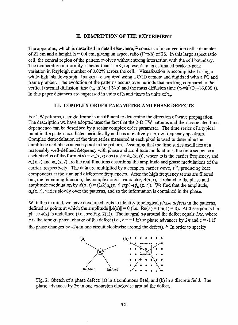
H. DESCRIPTION OF THE EXPERIMENT

The apparatus, which is described in detail elsewhere,12 consists of a convection cell a diameterof21 cm and a height, h = 0.4 cm, giving an aspect ratio (17=r/h) of 26. In this large aspect ratio

cell, the central region of the pattern evolves without strong interaction with the cell boundary.The temperature uniformity is better than 1 mK, representing an estimated peak-to-peakvariation in Rayleigh number of 0.02°/0 across the cell. Visualization is accomplished using awhite-light shadowgraph. Images are acquired using a CCD camera and digitized with a PC andframe grabber. The evolution of the atterns occurs over periods that are long compared to the

?vertical thermal diffusion time (~O=h/K=l 24s) and the mass diffision time (~c=h2/DC=:16,000 s).

In this paper distances are expressed in units of h and times in units of %O.

III. COMPLEX ORDER PARAMETER AND PHASE DEFECTS

For TW patterns, a single frame is insufllcient to determine the direction of wave propagation.The description we have adopted uses the fact that the 2-D TW patterns and their associated timedependence can be described by a scalar complex order parameter. The time series of a typicalpoint in the pattern oscillates periodically and has a relatively narrow frequency spectrum.Complex demodulation of the time series measured at each pixel is used to determine theamplitude and phase at each pixel in the pattern. Assuming that the time series oscillates at areasonably well-defined frequency with phase and amplitude modulations, the time secpence ateach pixel is of the form a(x)= aa(x, t) cos (cot+ $0(x, t)), where cois the carrier frequency, andao(x, t) and @@(x, t) are the real fimctions describing the amplitude and phase modulations of the

carrier, respectively. The data are multiplied by a complex carrier wave, eid, producing beat

components at the sum and difference frequencies. After the high frequency terms are filteredout, the remaining function, the complex order parameter, A(x, t), is related to the phase andamplitude modulation by A(x, t) = (1/2)a@(x, t) exp( -i@@ (x, t)). We find that the amplitude,aa(x, t), varies slowly over the patterns, and so the information is contained in the phase.

With this in mind, we have developed tools to identify topological pluzse defects in the patterns,defined as points at which the amplitude IIA(x)[I= O (i.e., Re(A) = Ire(A) = O). At these points thephase @(x) is undefined (i.e., see Fig. 2(a)). The integral d@around the defect equals 2.m, where

c is the topographical charge of the defect (i.e., c =+1 if the phase advances by 2Z and c = -1 if

the phase changes by -2z in one circuit clockwise around the defect). 16 In order to speci~

(a) (b)””.oo~o

,m~=o Z

● oeoooo

Fig. 2. Sketch of a phase defect (a) in a continuous field, and (b) in a discrete fielcl. Thephase advances by 27cin one excursion clockwise around the defect.

52

every defect in the pattern, the topological charge at each pixel is calculated using a loopconsisting of the eight surrounding pixels, as shown in Fig. 2(b), and then stored in a chargemap. Generally, the defects lie between pixels and are contained by loops centered on fouradjacent pixels, as indicated by the unshaded lattice points in Fig 2(b). Therefore, we identi~any connected group of pixels with the same nonzero topological charge as a single defect. Thedata presented here are sampled at a resolution of at least 14 pixels per wavelength, and for thissampling rate, the error rate in identi~ing phase defects is extremely low.

IV. RELAXATION OF TURBULENT STATES

We studied the time development of initially turbulent states to try to determine whatcharacterizes the evolution to more ordered patterns. Disordered states, such as that shown inFig. 3 (a), were generated by making a sudden jump in Rayleigh number.

Fig. 3. Traveling-wave convection patterns, represented by the phase of the complexamplitude, at several stages of the evolution of the pattern from a turbulent initial state.The elapsed time from the initiation of convection is given for each of the four images.White to black corresponds to the phase change 0- 2m

Fig. 4 shows the contours of the phase fields corresponding to the patterns in Fig. 3 at four timesduring the relaxation of a pattern. The crossings of Re(A) = Oand Ire(A) = Odetermine thepositions of the phase defects. The resulting arrays of defects, corresponding to the patterns inFig. 3, are shown in Fig. 5. The motion of the individual defects in Fig. 5 is shown by the graytails on the defects.

A key question is what determines the characteristic evolution of this pattern from an initiallydisordered state to a more ordered one and what limits the degree to which the patterns order. Asthe pattern evolves, the knots of phase contours are found to disentangle themselves, forming an

array of parallel lines that cross the minimum number of times necessary to satis~ the boundary

conditions. IS The end result is a pattern with several large domains of traveling waves, separatedby distinct, stable domain boundaries. In the defect description, the annihilation of defkct-antidefect pairs results in the minimal number of like-sign defects necessary to satisfy the

boundary conditions, leading to mature patterns such as the one shown in Figs. 3 (d) and 4(d). 13

II

Fig. 4. Contours of Re(A)=O and Im(A)=O are marked by black and grey lines for the—patterns shown in the four panels of Fig. 3.

We have found that the patterns continue to evolve until the net charge grows from the statisticalvariation in the initial number of defects (e.g., from 20-30 out of a total of- 600-1,000defects) to a value of approximately 72. This value of 72 is the number of defects that would beexpected if all of the rolls at the cell boundary orient perpendicular to the boundary. In this case,each roll pair terminates within the pattern, which is the configuration observed in ourexperiments. We concluded that the guiding principle that determines the pattern evolution isthe dominance of the long-range effect of the cell boundaries. Rolls orient approximatelyperpendicular to the cell walls, and sources of traveling waves are unstable. Thus all wavestravel in the same direction, resulting in global rotation of the pattern. The net charge of 72

54

.

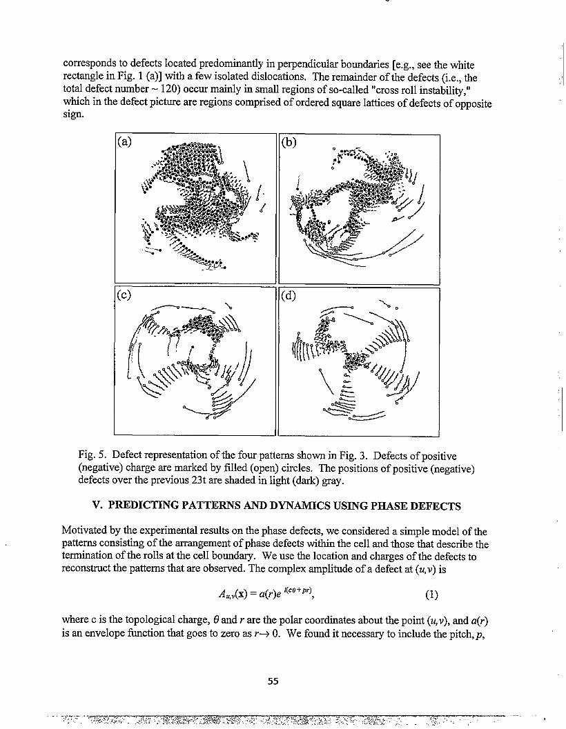
corresponds to defects located predominantly in perpendicular boundaries [e.g., see the whiterectangle in Fig. 1 (a)] with a few isolated dislocations. The remainder of the defects (i.e., thetotal defect number - 120) occur mainly in small regions of so-called “cross roll instability,”which in the defect picture are regions comprised of ordered square lattices of defects of oppositesign.

(

(

:a) (b)

Fig. 5. Defect representation of the four patterns shown in Fig. 3. Defects of positive(negative) charge are marked by filled (open) circles. The positions of positiv~ (negative)defects over the previous 23t are shaded in light (dark) gray.

V. PREDICTING PATTERNS AND DYNAMICS USING PHASE DEFECTS

Motivated by the experimental results on the phase defects, we considered a simple model of thepatterns consisting of the arrangement of phase defects within the cell and those that describe thetermination of the rolls at the cell boundary. We use the location and charges of the defects toreconstruct the patterns that are observed. The complex amplitude of a defect at (u,v) is

A.,,(x) = a(r)e ‘(co+Pr), (1)

where c is the topological charge, 0 and r are the polar coordinates about the point (u,v), and a(r)

is an envelope function that goes to zero as r+ O. We found it necessary to include the pitch, p,

55

which is a radial wave number that gives the phase a spiral-shaped appearance. The pattern as awhole is given by

A(x) = n.,, Au,,(x), (2)

which is just the sum of the phases of each defect, either in the pattern or at the domain

boundary, where the roll pairs terminate.17 Fig. 6 compares an actual pattern, the correspondingarray of defects, and the pattern reconstructed using the above formalism and a non-zero pitch.A value of p = 0.0 Ih-l was found to be necessary, so that the orientation of waves near domainboundaries matches that of the observed pattern. Forp = O,waves make approximately equalangles to domain boundaries, instead of the angles of 0° and 90° that are observed. Theremaining differences between the patterns predicted and observed are due mainly to the fact thatthe wave number of the experimental patterns is very rigid, with k varying less than *1 O% across

the convection cell. As illustrated”by the right-hand panel in Fig. 6, wave number rigidity is notcontained in the point defect model. Thus, an additional (and at this point unspecified)

mechanism, such as phase diffusion, will be necessary to keep the wave number constant. 1gWith this caveat, the arrangement of point defects describes the patterns relatively accurately.

Fig. 6. The phase of the complex amplitude of a mature TW pattern is shown on the left.In the center, defects of positive (negative) topological charge for this pattern are denotedby open (filled) circles. The reconstruction of the pattern based on these defects andusing p=-O.Olb-l is shown on the right.

We have begun to consider what determines the motion of the defects as a way to address thedynamics of the patterns. We developed a technique to measure the phase field upon which thedefects are superimposed. Using this technique, we find that we are able to correlate the defectvelocity, v& with the magnitude and direction of the gradient in this phase at the defect, whichwe denote by the wave vector ~. The resulting expression is

vd = @Q + ~c(kd x z), (3)

where ~ and q are constants and c is the topological charge of the defect. The second term in the

equation differs from that which would be expected in stationary convection. In that cme, climbof a dislocation is a mechanism for wave number selection, and the motion of dislocations in theroll direction is proportional to h - h, where b is the preferred wave number of the piittern.

56

VI. CONCLUDING REMARKS

The phase defect description of traveling wave patterns appears to be a promising approach todescribing traveling-wave patterns and dynamics. The key to this research is that convection inmixtures is a model system for studying phase turbulence -- one in which the order parametercan be measured with sufficient precision to identifi and track the phase defects accurately. Wehave tried to determine the extent to which the traveling-wave patterns and their dynamics can bedescribed solely in terms of the phase defects. We are now focusing on questions regardingdefect motion. One open question is what determines the parameters ~ and q in Eq. 3. Our first

intuition is that q could be related to the circular geometry of the convection cell, and in

particular, to the curvature of the cell walls (e.g., perhaps due to mean flows). A second questionis what determines the pitch, p, of”the defects. We plan to pursue these topics in futureexperiments.

VII. ACKNOWLEDGEMENT

This work is supported by the Department of Energy Grant DE-FG09-90ER14148.

REFERENCES

* Present address: Laboratory of Atomic and Solid State Physics, Cornell University,Ithaca NY 14853

1

2

3

4

5

6

7

8

9

10

11

12

13

14

15

16

17

18

E. N. Lorenz, J. Atmos. Sci. 20,230 (1963).

J. Murray, Nonlinear Dl~erential Equation Models in Biology, Clarendon Press (1997).

R. E. Ecke, Y. Hu, R. Mainieri, et al., Science 269, 1704-7 (1995).

G. W. Baxter, R. P. Behringer, T. Fagert, et al., Phys. Rev. Lett. 62,2825 (1989).

P. Coullet, L. Gil, and F. Rocca, Optics Comm. 73,403-8 (1989).

J. Lega, J. V. Maloney, and A. C. Newell, Phys. Rev. Lett. 73,2978-81 (1994).

E. Pampaloni, P. L. Rarnazza, S. Residori, et al., Phys. Rev. Lett. 74,258-61 (1994).

M. C. Cross and P. C. Hohenberg, Rev. Mod. Phys. 65 (1993).

P. Manneville, Dissipative Structures and Weak Turbulence, Academic Press (1990).

R. W. Walden, P. Kolodner, A. Passner, et al., Phys. Rev. Lett. 55 (1985).

W. Barten, M. Lticke, W. Hort, et al., Phys. Rev. Lett. 63,376-79 (1989).

A. La Porta and C. M. Surko, Phys. Rev. E 53,5916-34 (1996).

A. La Porta and C. M. Surko, Phys. Rev. E 56,5351-66 (1997).

A. La Porta and C. M. Surko, Phys. Rev. Lett. 77,2678-81 (1996).

P. Kolodner, M. Williams, and C. Moe, J. Chem. Phys. 88,6512 (1988).

A. C. Newell, T. Passot, and J. Lega, Ann. Rev. Fluid Mech. 25,399 (1993).

A. La Porta and C. M. Surko, Phys. Rev. Lett. 80,3759-62 (1998).

G. D. Granzow and H. Reicke, Physics A 249,27-35 (1998).

SPATIOTEMPORAL PATTERNS IN VERTICALLY VIBRATED GRANULARLAYERS: EXPERIMENT AND SIMULATION

M. D. Shattuck, C. Bizon, J. B. Swift and Harry L. Swinney

Center for Nonlinear Dynamicsand Department of Physics

The University of Texas at AustinAustin, TX 78712

ABSTRACT

Thin layers of vertically vibrated granular media lose stability to sub-harmonic standingwave patterns when the driving acceleration is increased above a critical value of about 2.5times gravity. Space filling patterns, squares, stripes, and hexagons are observed for differ-ent values of the two control parameters, frequency and acceleration. Localized structures(oscillons), are also observed for a small range of control parameters. Event driven molec-ular dynamics simulations reproduce all of the space filling patterns at the same controlparameters as in the experiments, and yield the pattern wavelength as a function of driv-ing frequency to within a few percent. The simulation allows many important propertiesof granular flows to be determined which are difficult or impossible to measure in kLbora-tory experiments, such as, velocity distribution functions, velocity fields, and the granulartemperature. It offers a first step toward verification of rigorous theories of granular flowsbased on kinetic theory.

INTRODUCTION

Transport and processing of granular materials is important in industries ranging from food prepa-ration to pharmaceuticals to coal processing. However, theoretical understanding of granular flowshas lagged significantly behkd liquid and gas flows. No basic theory of granular flows comparableto the Navier-Stokes equations for fluids has attained widespread acceptance[l], and it has beenargued that such a theory is not possible[2]. Thk lack of understanding leads to significant waste insolids processing. One study found that in commercial processing plants with solid feed stock theaverage operating capacity was 64% of design capacity, compared with an industry standard of 90to 9570 of design capacity for plants with liquid or gas feed stock[3]. An increased understandingof granular flows could improve this situation. The goal of our current research in granular materi-als is to elucidate and test basic granular theories with high precision experiments and moleculardynamics simulations.

Recent experiments[4, 5, 6] show pattern formation in vertically vibrated granular layers whichis strikingly similar to patterns seen in fluid systems (see Figure 1). This similarity suggests that

58

in this system, equations of motion similar to Navier-Stokes could be found. Equations similar toNavier-Stokes have been derived from kinetic theory for granular media flows under the assumptionof binary hard sphere collisions and in the limit of small energy loss in collisions[7, 8, 9, 10, 11, 12].These theories produce equations that differ slightly from the dense gas Navier-Stokes equations bythe addition of a temperature loss rate term in the energy equation, in the form of the constitutiverelations for shear and bulk viscosity and thermal conductivity, and in the equation of state for thepressure. In these equations the granular temperature is not the thermodynamic temperature butby analogy to molecular gases is the average of the square of the deviations of the velocity horn themean velocity (i.e., the variance of the velocity). While these equations have been available for 25years there have been few experimental[13, 14, 15] or numerical[16, 17, 18, 19] tests. This deficiencymay be due to the fact that many granular flows do not show obvious fluid-like behaviors becauseinelasticity of the particle collisions drives the granular temperature very low.

Ex~eriment

(a)

r=3.00

{=0.27

(b)r=3.00

{=0.44

(c)

r=4.00

f=O.38

(d)r=4.00

{=0.38

Simulation

(e)

r=5.00

{=0.44

(f)

r=5.79

{=0.47

(9)r=6.oo

{=0.84

(h)

r=7.00

{=0.75

Ex~eriment Simulation

Figure 1. Comparison of standing wave patterns obtained in experiment and simulation: (a)squares, (b) stripes, (c) and (d) alternating phases of hexagons, (e) flat, (f) squares, (g) stripes,(h) hexagons. (a)-(e) oscillate at j/2 and (f)-(h) oscillate at ~/4. The layer depth is 5.42 particlediameters. The experiments use lead spheres sieved between 0.5 and 0.6 mm in a container whichis 100 particle diameters on each side.

59

Experiments in vibrated layers of granular materials provide an unprecedented opportunity tostudy granular fluid-like behavior. However, experiments alone do not provide information on themicroscopic underpinnings of the kinetic theory description, due to the difficulty of internal mea-surements in three dimensional systems. To overcome this difficulty we have developed an eventdriven molecular dynamics simulation capable of quantitatively reproducing our experiments[20],including wavelength changing secondary instabilities [21]. The simulation is based on ~sumptionssimilar to those for granular kinetic theory. In particular, particles obey Newton’s laws between bi-nary instantaneous collisions (hard sphere model) which conserve momentum, but dissipate energy.However, unlike the kinetic theory models the energy dissipation can be large. Using this simulationwe have also found enhanced diffusion perpendicular to the stripe patterns and internal convectionrolls in all of the pattern states[22].

I

DigitalCamera

/ \ II/ \

GranularMaterial

DigitalFunctionElectro- GeneratorMechanicalshaker

?

AmplifierI I I I

(a)

r5 -

4 -

3 -

2 -

o(e) flat (f/2)

...hexagons (f/2) ~

flat

o 0.5 1

<

(b)

Figure 2. (a) Schematic of the experimental apparatus showing the container, the shaker and theimaging system. The camera can be placed above, to produce images like those in Figure 1, or tothe side of the test cell, to produce images like those in the top of Figure 3(b). Phase diagram fromthe experiments for layer depth of 5.71 particles. The parameter values used for the patterns inFigure 1 are indicated by (a) through (h). Solid lines denote the transitions with increasing 17,anddotted lines denote transitions for decreasing I’. Shaded areas show transitional regiorls betweenstripes and squares.

EXPERIMENTAL APPARATUS

The experiment consists of an evacuated container filled with a thin layer of particles (2-30 particlediameters deep) and vibrated sinusoidally (A sin(2m~i)) in the vertical direction by an industrialelectro-mechanical shaker (see Figure 2(a)). Evacuation eliminates a heaping instability caused byinteraction of the grains with the interstitial gas[23]. The top and sides of the cent airier are trans-

parent for visualization by a high speed digital camera and the bottom is aluminum. Many differenttypes of particles (e.g., bronze, lead, glass, plastic, rice, etc.) and diameters (0.05–3 mm) have beenused and produce qualitatively similar results. The control parameters are the acceleration ampli-tude A, varied up to 1 cm, and the frequency f, varied from 10 to 200 Hz. Experiments are typicallyperformed at constant 17 = 2mAf2/g, where g is the gravitational acceleration constant, and f is

60

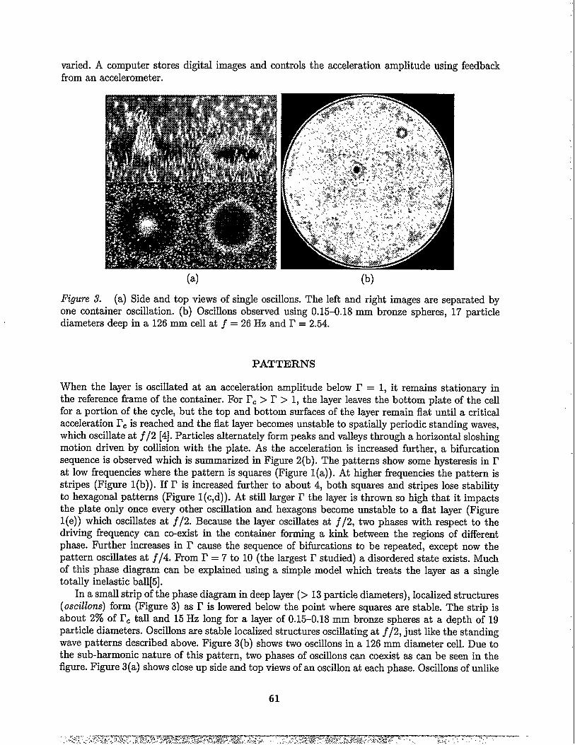
varied. A computer stores digital images and controls the acceleration amplitude using feedbackhorn an accelerometer.

Figure 3.

(a) (b)

(a) Side and top views of single oscillons. The left and right images are separated byone container” oscillation. (b) Oscillons observed using 0.15–0.18 mm-bronze-spheres, i7 particiediameters deep in a 126 mm cell at f =26 Hz and 17= 2.54.

PATTERNS

When the layer is oscillated at an acceleration amplitude below 17= 1, it remains stationmy inthe reference fkame of the container. For rc > I’ >1, the layer leaves the bottom plate of the cellfor a portion of the cycle, but the top and bottom surfaces of the layer remain flat until a criticalacceleration 17Cis reached and the flat layer becomes unstable to spatially periodic standing waves,which oscillate at j/2 [4]. Particles alternately form peaks and valleys through a horizontal sloshingmotion driven by collision with the plate. As the acceleration is increased further, a bifurcationsequence is observed which is summarized in Figure 2(b). The patterns show some hysteresis in I’at low frequencies where the pattern is squares (Figure 1(a)). At higher frequencies the pattern isstripes (Figure 1(b)). If I’ is increased further to about 4, both squares and stripes lose stabilityto hexagonal patterns (Figure 1(c,d)). At still larger r the layer is thrown so high that it impactsthe plate only once every other oscillation and hexagons become unstable to a flat layer (Figurel(e)) which oscillates at ~/2. Because the layer oscillates at f/2, two phases with respect to thedriving frequency can co-exist in the container forming a kink between the regions of differentphase. Further increases in r cause the sequence of bifurcations to be repeated, except now thepattern oscillates at f/4. From I’ = 7 to 10 (the largest I’ studied) a disordered state exists. Muchof this phase diagram can be explained using a simple model which treats the layer as a singletotally inelastic ball[5].

In a small strip of the phase diagram in deep layer (> 13 particle diameters), localized structures(oscilkms) form (Figure 3) as I’ is lowered below the point where squares are stable. The strip isabout 2% of rc tall and 15 Hz long for a layer of 0.15–0.18 mm bronze spheres at a depth of 19particle diameters. Oscillons are stable localized structures oscillating at f/2j just like the standingwave patterns described above. Figure 3(b) shows two oscillons in a 126 mm diameter cell. Due tothe sub-harmonic nature of this pattern, two phases of oscillons can coexist as can be seen in thefigure. Figure 3(a) shows close up side and top views of an oscillon at each phase. Oscillons of unlike

61

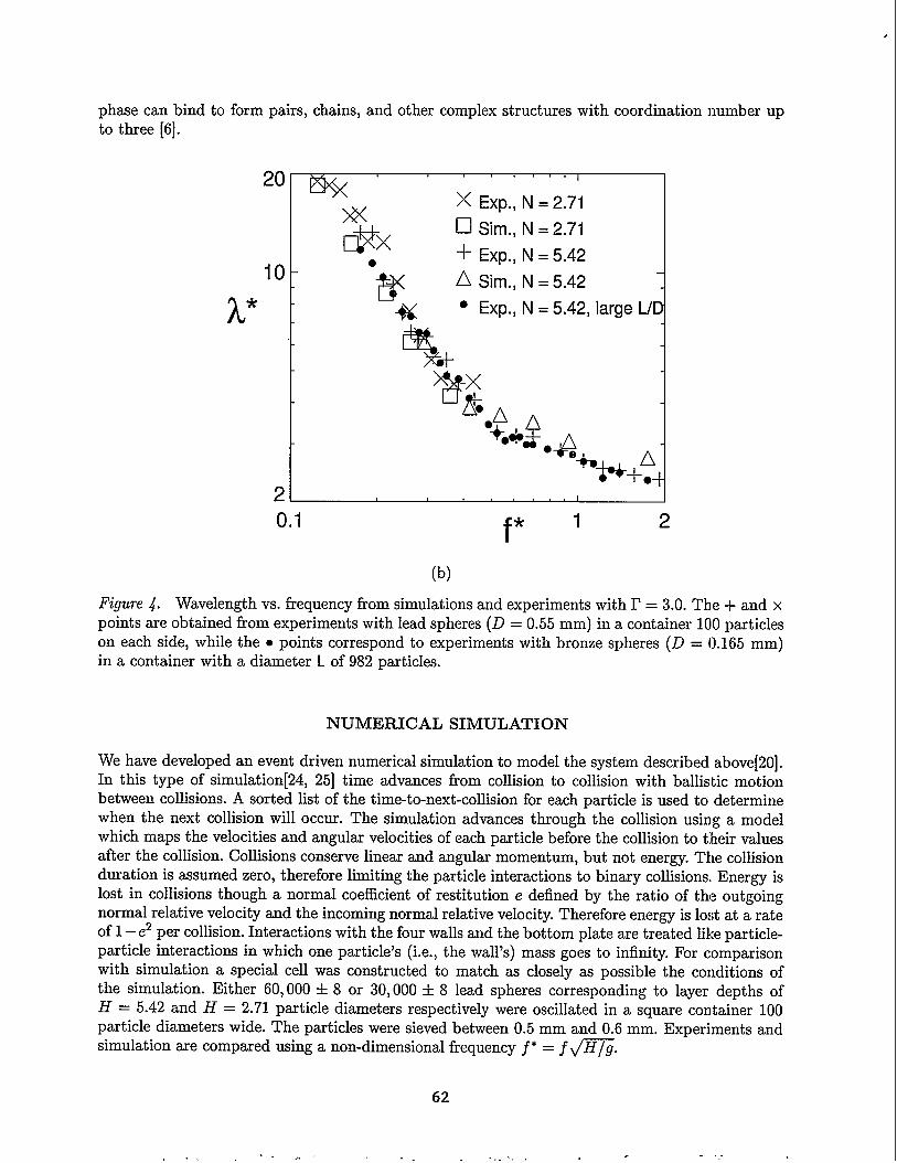
phase can bind to form pairs, chains, and other complex structures with coordination number upto three [6].

20

10

20.1

x Exp., N = 2.71%

&x❑ Sire., N = 2.71

+ Exp., N = 5.42●

B~ Sire., N = 5.42

* ● Exp., N = 5.42, large L/

%

f* 1 2

(b)

Figure 4. Wavelength vs. frequency from simulations and experiments with I’ = 3.0. The + and xpoints are obtained from experiments with lead spheres (D = 0.55 mm) in a container 100 particleson each side, while the . points correspond to experiments with bronze spheres (D = 0.165 mm)in a container with a diameter L of 982 particles.

NUMERICAL SIMULATION

We have developed an event driven numerical simulation to model the system described above[20].In this type of simulation[24, 25] time advances from collision to collision with ballistic motionbetween collisions. A sorted list of the time-to-next-collision for each particle is used to determinewhen the next collision will occur. The simulation advances through the collision using a modelwhich maps the velocities and angular velocities of each particle before the collision to t:heir valuesafter the collision. Collisions conserve linear and angular momentum, but not energy. The collisionduration is assumed zero, therefore limiting the particle interactions to binary collisions. Energy islost in collisions though a normal coefficient of restitution e defined by the ratio of the outgoingnormal relative velocity and the incoming normal relative velocity. Therefore energy is lost at a rateof 1– e2 per collision. Interactions with the four walls and the bottom plate are treated like particle-particle interactions in which one particle’s (i.e., the wall’s) mass goes to infinity. For comparisonwith simulation a special cell was constructed to match as closely as possible the conditions ofthe simulation. Either 60,000 + 8 or 30,000 + 8 lead spheres corresponding to layer depths ofH = 5.42 and H = 2.71 particle diameters respectively were oscillated in a square container 100particle diameters wide. The particles were sieved between 0.5 mm and 0.6 mm. Experiments andsimulation are compared using a non-dimensional frequency ~’ = f~.

,.

62

. . .

I

Three collisional particle properties — the coefficient of friction p, the normal coefficient ofrestitution e, and the cutofl for the rotation coefficient of restitution PO — must be determinedfor the simulation. f?. is taken from the literature[26]. e and p are determined by adjusting theirvalues until the pattern wavelength in the simulation and experiment matched in two specific runs,I’= 3.0, j“ = 0.205, H = 2.71 (for e), and I’ = 3.0, i* = 0.534, H = 5.42 (for p). By this procedurethe value of e is set to 0.7 and p to 0.5. However, the values of these parameters do not stronglyeffect the qualitative behavior of the simulation, only the quantitative agreement. For example, achange in e from 0.5 to 0.8 only changes the observed wavelength of the pattern by 30Y0,the patternplanform is not effected.

The results of the simulation for various control parameters are shown in Figure 1. Patternsare obtained in the simulation and experiment at the same values of control parameters which aredenoted by points on the phase diagram (Figure 2(b)) labeled (a)-(h). Both j/2 (a)-(e) and ~/4(f)-(h) patterns show a striking correspondence. Further, the pattern wavelengths for various f“,in experiment and simulation agree well, even when comparing the simulation in a cell 100 particlediameters wide with experiments in a large container with a diameter of 982 particle diameters(Figure 4).

Currently, simulations have not reproduced stable oscillons. However due to the extremely smallrange of stability and the layer depths required, this is not surprising. The computational timedepends of the square of the depth, which makes the search intractable with the current code.

DISCUSSION

Using this simulation we have also determined properties of the vibrated granular system whichcan not be easily measured in the experiment. For example we have found enhanced diffusion ofparticles perpendicular to the stripe pattern direction (i.e., from peak to peak), and discovered aconvective roll pattern within each peak and valley of the pattern[22]. The convective roll patternis a prediction of the simulation, but has not been verified experimentally. Anisotropic diffusion isalso seen in other fluid systems as a result of advection (e.g., Rayleigh-B&mrd convection).

de Bruyn et al.[21] describe another similarity of granular pattern formation to Rayleigh-B&mrdconvection. Wavelength changing secondary instabilities define a wavenumber stability region be-tween cross-roll and skew-varicose instabilities. Event driven simulations show the same instabilitiesand allow the calculation of average vertical vorticity which is shown to be large only during a skew-varicose instability just as in the fluid case[21].

The good agreement between simulation and experiment validates the assumptions of the sim-ulation model. The basic assumptions of the model are that particles follow Newton’s law betweencollisions, and collisions are binary, conserve momentum, and dissipate energy. These are the sameassumptions of granular kinetic theory [7, 8, 9, 10, 11, 12], with the add~tion that the energy loss anddensity are small and that there are no velocity correlation. To further test the ideas of granularkinetic theory we have performed two-dimensional simulations of a granular gas of inelastic harddisks, driven uniformly by a heat bath[18, 19]. This system was chosen as our first test becausedirect comparison with the transport coefficients can be made with the values calculated analyti-cally from granular kinetic theory. We find that although velocity correlations do exist [19] granulzukinetic theory describes the system well even for strong dissipation, high densities, and small num-bers of particles[18]. Specifically, for e = 0.7, which corresponds to about half of the energy lostper collision, densities up to 0.75 volume fiactionj and a system size of 52.6 particle diameters, theenergy loss rate and the shear viscosity deviate by less than 20Y0, and the thermal conductivitydeviates by less than 50%. For all transport coefficients, the deviation from kinetic theory improvesif dissipation and density are decreased, in accord with the assumption that they are small. Thegeneral level of agreement is surprisingly good considering that the density and energy loss per

63

collision is so high, and suggests that a continuum approach may be able to quantitatively as wellas qualitatively describe some granular systems.

ACKNOWLEDGEMENTS

This research is supported by the U.S. Department of Energy Office of Basic Energy Sciences.

REFERENCES

1.

2.

3.

4.

5.

6.

7.

8.

9.

10.

11.

12.

13.

14.

15.

H. M. JAEGER, S. R. NAGEL, and R. P. BEHRINGER, “The Physics of Granular Material,”Physics Today, 432-38 (1996).

L. P. KADANOFF, “Built Upon Sand: Theoretical Ideas Inspired by the Flow of GranularMaterials,” Rev. Mod. Phys., ‘~ 435-444 (1999).

E. W. MERROW, “Linking R&D to Problems Experienced in Solids Processing,” Chem. Eng.Progress, u 14 (1985).

F. MELO, P. UMBANHOWAR, and H. L. SWINNEY, “Transition to Parametric Wave Pat-terns in a Vertically Oscillated Granular Layer, “ Phys. Rev. Lett., ~ 172-175 (1994).

F. MELO, P. B. UMBANHOWAR, and H. L. SWINNEY, “Hexagons, Kinks, and Disorder inOscillated Granular Layers,” Phys. Rev. Lett., E 3838-3841 (1995).

P. UMBANHOWAR, F. MELO, and H. L. SWINNEY, “Localized Excitations in a VerticallyVibrated Granular Layer,” Nature, W 793-796 (1996).

J. T. JENKINS and M. W. RICHMAN, “Grad’s 13-moment system for a dense gas of inelasticparticles,” Arch. Rat. Mech. Anal., &7 355-377 (1985).

J. T. JENKINS and S. B. SAVAGE, “A theory for the rapid flow of identical, smooth, nearlyelastic particles: J. Fluid Mech., W 187-202 (1983).

C. K. K. LUN, S. B. SAVAGE, D. J. JEFFREY, and N. CHEPURNIY, “Kinetic theories forgranular flow: inelastic particles in Couette flow and slightly inelastic particles in a generalflowfield~ J. Fiuid Mech., W 223-56 (1983).

C. K. K. LUN and S. B. SAVAGE, “The effects of an impact velocity dependent coefficientof restitution on stresses devloped by sheared granular materials,” Acts Mechanica, ~ 15–44(1986).

C. K. K. LUN, “Kinetic theory for granular flow of dense, slightly inelastic, slightly roughspheres,” J. Fluid Mech., &J3 539-559 (1991).

A. GOLDSTEIN and M. SHAPIRO, “Mechanics of Collisional Motion of Granular Materials.Part 1. Gene ral hydrodynamic equations,” J. Fluid Mech., 282 75–114 (1995).

T. G. DRAKE, “Granular flow: physical experiments and their implications for microstructuraltheories.,” J. Fluid Mech., W 121-152 (1991).

J. DELOUR, A. KUDROLLI, and J. P. GOLLUB, “Velocity distributions in vertically vi-brated granular media: preprint (1998).

J. S. OLAFSEN and J. S. URBACH, “Clustering, order, and collapse in a driven granularmonolayer,” Phys. Rev. Lett., U 4369-72 (1998).

64

. .

16.

17.

18.

19.

20.

21.

22,

23.

24.

25.

26.

C. S. CAMPBELL, “Rapid Granular Flows,” Annu. Rev. Fluid Mech., z 57-92 (1990).

E. L. GROSSMAN, T. ZHOU, and E. BEN-NAIM, “Towards granular hydrodynamics in twodimensions,” Phys. Rev. E, &j 4200 (1997).

C. BIZON, M. D. SHATTUCK, J. B. SWIFT, and H. L. SWINNEY, “Transport Coefficientsfor Granular Media from Molecular Dynamics Simulations,” Submitted to Phys. Rev. E (1999).

C. BIZON, M. D. SHATTUCK, J. B. SWIFT, and H. L. SWINNEY, “Velocity correlationsin driven two-dimensional granular media,” In Dynamics: Models and Kinetic Methods forNonequilibrium Many-Body Systems, J. KARKHECK, cd., NATO ASI Series E. Applied Sci-ences (Kluwer Academic publishers, Dordrecht, 1999).

C. BIZON, M. D. SHATTUCK, J. B. SWIFT, W. D. MCCORMICK, and H. L. SWINNEY,“Patterns in 3D Vertically Oscillated Granular layers: Simulation and Experiment,” Phys.Rev. Lett., ~ 57-61 (1998).

J. R. DE BRUYN, C. BIZON, M. D. SHATTUCK, D. GOLDMAN, J. B. SWIFT, and H. L.SWINNEY, “Continuum-type stability balloon in oscillated granular layers,” Phys. Rev. Lett.,~ 1421-1424 (1998).

C. BIZON, M. D. SHATTUCK, J. R. DE BRUYN, J. B. SWIFT, W. D. MCCORMICK,and H. L. SWINNEY, “Convection and Diffusion in Vertically Vibrated Granular Pa-terns~ J. Stat. Phys., ~ 449 (1998), Color pictures of granular convection can be foundat http: //chaos. ph.utexas.edu/errata/bizon98a.html.

H. K. PAK, E. VAN DOORN, and R. P. BEHRINGER, “Effects of Gases on Granular Mate-rials under Vertical Vibration,” Phys. Rev. Lett., M 4643–4646 (1995).

M. MARiN, D. RISSO, and P. CORDERO, “Efficient Algorithms for Many-Body Hard Par-ticle Molecular Dynamics: J. Comput. Phys., w 306-317 (1993).

B. D. LUBACHEVSKY, “How to Simulate Billiards and Similar Systems,” J. Comp. Phys.,~ 255-283 (1991).

O. R. WALTON, “Numerical Simulation of Inelastic, Frictional Particle-Particle Interactions,”in Particulate Two-Phase Flow, M. C. ROCO, cd., (Butterworth-Heinemann, Boston, 1993),pp. 884-911.

proceedings of the seventeenth symposium on energy ...€¦ · proceedings of the seventeenth...

Documents