proceedings of the ecrypt workshop on tools for cryptanalysis 2010

Proceedings of the ECRYPT Workshop on

Tools for Cryptanalysis 2010

Francois-Xavier Standaert (Ed.)

22 – 23 June 2010,Royal Holloway, University of London, Egham, UK

Organised by ECRYPT II - Network of Excellence in Cryptology II

Programme Chair

Francois-Xavier Standaert Universite catholique de Louvain, Belgium

Programme Committee

Martin Albrecht Royal Holloway, University of London, UKFrederik Armkrecht Technical University of Darmstadt, GermanyAlex Biryukov University of Luxembourg, LuxembourgJoo Yeon Cho Nokia A/S, DenmarkChristophe de Canniere Katholiek Universiteit Leuven, BelgiumSerge Fehr Centrum Wiskunde & Informatica, CWI, The NetherlandsTim Guneysu Ruhr Universitat Bochum, GermanyTanja Lange Technische Universiteit Eindhoven, The NetherlandsArjen Lenstra Ecole Polytechnique Federale de Lausanne, SwitzerlandAlexander May Ruhr Universitat Bochum, GermanyFlorian Mendel Graz University of Technology, AustriaMarine Minier Institut National des Sciences Appliquees de Lyon, FranceLudovic Perret LIP6-UPMC, Universite de Paris 6 & INRIA, FranceGilles Piret Oberthur Technologies, FranceDamien Stehle CNRS, University of Sydney and Macquarie University, AustraliaMichael Tunstall University of Bristol, UKNicolas Veyrat-Charvillon Universite catholique de Louvain, Belgium

ASCAtoCNF — Simulating Algebraic Side-Channel Attacks 9

Mathieu Renauld

Automated Algebraic Cryptanalysis 11

Paul Stankovski

Tools for Algebraic Cryptanalysis 13

Martin Albrecht

Hybrid Approach: a Tool for Multivariate Cryptography 15Luk Bettale, Jean-Charles Faugere and Ludovic Perret

Sieving for Shortest Vectors in Ideal Lattices 25

Michael Schneider

Time-Memory and Time-Memory-Data Trade-Offs for Noisy Ciphertext 27Marc Fossorier, Miodrag Mihaljevic and Hideki Imai

Algebraic Precomputations in Differential Cryptanalysis 37Martin Albrecht, Carlos Cid, Thomas Dullien, Jean-Charles Faugere and Ludovic Perret

SYMAES: A Fully Symbolic Polynomial System Generator for AES-128 51Vesselin Velichkov, Vincent Rijmen and Bart Preneel

Efficient Decomposition of Dense Matrices over GF(2) 53

Martin Albrecht and Clement Pernet

Breaking Elliptic Curves Cryptosystems using Reconfigurable Hardware 71Junfeng Fan, Daniel V. Bailey, Lejla Batina, Tim Guneysu, Christof Paar and Ingrid Ver-bauwhede

Fast Exhaustive Search for Polynomial Systems in F2 85Charles Bouillaguet, Hsieh-Chung Kevin Chen, Chen-Mou Cheng, Tony (Tung) Chou, RubenNiederhagen and Bo-Yin Yang

Links Between Theoretical and Effective Differential Probabilities: Experiments onPRESENT 109

Celine Blondeau and Benoit Gerard

Toolkit for the Differential Cryptanalysis of ARX-based CryptographicConstructions 125

Nicky Mouha, Vesselin Velichkov, Christophe De Canniere and Bart Preneel

KeccakTools 127Guido Bertoni, Joan Daemen, Michael Peeters and Gilles Van Assche

The CodingTool Library 129

Tomislav Nad

4

Grain of Salt - An Automated Way to Test Stream Ciphers throughSAT Solvers 131

Mate Soos

Analysis of Trivium by a Simulated Annealing Variant 145Julia Borghoff, Lars Knudsen and Krystian Matusiewicz

5

Preface

The focus of this workshop is on all aspects related to cryptanalysis research, mixing symmetricand asymmetric cryptography, as well as implementation issues. The workshop is a forum forpresenting new software and hardware tools, including their underlying mathematical ideas andpractical applications. Topics of interest include (but are not limited to):

• The automatic search of statistical trails in block ciphers.

• Lattice reduction and its application to the cryptanalysis of asymmetric encryption schemes.

• Fast HW and SW implementations for cryptanalysis (e.g. in FPGAs, graphic cards).

• Algebraic cryptanalysis (e.g. with SAT solvers, Grobner bases).

• Sieve algorithms for integer factorization.

• Time/memory/data/key tradeoffs and birthday paradox-based attacks.

• Fourier and Hadamard-Walsh transforms and their applications in cryptanalysis.

• Tools for the fast and efficient collision search in hash functions.

• Physical (e.g. side-channel, fault) attacks, in particular their computational aspects.

• Cryptanalysis with alternative models of computation (e.g. quantum, DNA).

Invited Talks

A primer on lattice reduction

Marc Joye, Technicolor, FranceLattice basis reduction has found numerous applications in various research areas. This talk aimsat giving a first introduction to the LLL algorithm. It explains how to use it to solve some simplealgorithmic problems. It also describes how to break several early cryptosystems. The talk ismainly intended to practitioners wanting to use LLL as a toolbox. No mathematical backgroundis required.

Factorization of a 768-bit RSA modulus

Paul Zimmermann, INRIA/LORIA, Nancy, FranceOn December 12, 2009, together with Kleinjung, Aoki, Franke, Lenstra, Thome, Bos, Gaudry,Kruppa, Montgomery, Osvik, te Riele and Timofeev, we have completed the factorization of RSA-768 by the number field sieve. This factorization took the equivalent of about 1700 years on a2.2Ghz AMD64 core. The talk will recall the main steps of the number field sieve, and will givethe corresponding figures for RSA-768.

7

ASCAtoCNF - Simulating Algebraic Side-ChannelAttacks

Mathieu Renauld?

UCL Crypto Group, Universite catholique de Louvain, B-1348 Louvain-la-Neuve.

e-mails: [email protected]

Abstract

Algebraic Side-Channel Attacks (ASCA) were recently presented ([1, 2]) as a new type ofattack against block ciphers that combines side-channel information (information deducedfrom a physical leakage, like the power consumption of the device) and classical crypt-analysis (in this case algebraic cryptanalysis). These attacks show interesting properties.Indeed, they can exploit all available side-channel information (a standard DPA exploitsonly the first/last round), and thus require a smaller data complexity than other side-channel attacks. It turns out that ASCA can succeed with a data complexity of 1 (only oneencryption measured), and even in an unknown plaintext/ciphertext context or against amasked implementation.

An ASCA can be divided in two phases. During the first online phase, the adversaryperforms measurements on the device during several encryptions. Then, during the secondoffline phase, the adversary translates the block cipher and the recovered side-channelinformation into a system of boolean equations, and tries to solve it. One of the possibletechniques to solve this system is to translate it into a satisfiability problem, and to use aSAT solver.

ASCAtoCNF is a tool that provides the user with a quick way to simulate an ASCAwith a data complexity of 1 to 9. The user specifies the target block cipher (PRESENT orthe AES), the plaintext and secret key used. To simulate the side-channel recovery phase,the user chooses which operations of the block cipher are leaking information (for example:all the substitution operations from round 5 to 9). The side-channel recovery phase isassumed to be perfect (all recovered side-channel information is correct), but the user canmake the attack harder by reducing the quantity of available side-channel information. Theleakage model is the Hamming weight model on 8 bits: the adversary is assumed to recoverthe Hamming weight values of the data processed by the device during the specified leakingoperations. The generated SAT problem can then be solved by a SAT solver like MiniSAT([3]). With this tool, one can easily try various configurations of known leakages and studythe impact of these configurations on the time complexity of the ASCA.

References

1. M. Renauld, F.-X. Standaert, Algebraic Side-Channel Attacks, in the proceedings of INSCRYPT2009, to appear.

2. M. Renauld, F.-X. Standaert, N. Veyrat-Charvillon, Algebraic Side-Channel Attacks on theAES: Why Time also Matters in DPA, in the proceedings of CHES 2009, LNCS, vol. 5747, pp.97-111, Lausanne, Switzerland, September, 2009.

3. MiniSAT, available online at http://minisat.se/.

? Work supported in part by the Walloon Region research project SCEPTIC.

9

Automated Algebraic Cryptanalysis

Paul Stankovski

Dept. of Electrical and Information Technology, Lund University,P.O. Box 118, 221 00 Lund, Sweden

Abstract. We describe a simple tool for automatic algebraic cryptanalysis of a largearray of stream- and block ciphers. Three tests have been implemented and the bestresults have led to continued work on a computational cluster. Our best results shownonrandomness in Trivium up to 1070 rounds (out of 1152), and in the full Grain-128with 256 rounds.

Keywords: algebraic cryptanalysis, maximum degree monomial test, automated testing

The core of this work is the Maximum Degree Monomial (MDM) test [1, 2], which we usefor algebraic cryptanalysis of a large array of stream and block ciphers. To facilitate time-ecient and automatic testing, we created a tool for running algebraic cryptanalysistests. We assembled several specialized implementations that output initialization data,which is necessary for the algebraic tests. A generic interface then provides uniformaccess to all primitives. Algebraic tests can be implemented generically and run foreach of the supported algorithms. This has been done for Trivium, Grain-128, Grain v1,Rabbit, Edon80, AES-128/256, DES, TEA, XTEA, SEED, PRESENT, SMS4, Camellia,RC5, RC6, HIGHT, CLEFIA, HC-128/256, MICKEY v2, Salsa20/12 and Sosemanuk.

We have implemented three particularly interesting tests. A greedy incarnation ofthe MDM test reveals inadequacies in bit mixing, and does so beautifully. This test canalso point out unexpected key weight anomalies. A bit-ip test was devised to catchsimple symmetry errors. Also, exhaustive search for small but optimal bit sets for theMDM test was also implemented.

The greedy approach to nding promising bit sets for the MDM test works ex-ceptionally well for Trivium and Grain-128 (compare to [3, 4]). Using a computationalcluster, we then pushed our computational limits to show weaknesses in Trivium re-duced to 1070 (out of 1152) initialization rounds. The greedy strategy also works wellfor Grain-128, revealing nonrandomness through all 256 initialization rounds.

Our vision is that every algorithm designer should use our or other similar testingtools during algorithm development to catch algebraic weaknesses earlier than what hasbeen possible before.

References

1. M.-J. O. Saarinen. Chosen-IV statistical attacks on eSTREAM stream ciphers. eSTREAM,ECRYPT Stream Cipher Project, Report 2006/013, 2006. http://www.ecrypt.eu.org/stream.

2. H. Englund, T. Johansson, and M. S. Turan. A framework for chosen IV statistical analysis ofstream ciphers. In K. Srinathan, C. Pandu Rangan, and M. Yung, editors, Progress in Cryptology

- INDOCRYPT 2007, volume 4859/2007 of Lecture Notes in Computer Science, pages 268281.Springer-Verlag, 2007.

3. J.-P. Aumasson, I. Dinur, L. Henzen, W. Meier, and A. Shamir. Ecient FPGA Imple-mentations of High-Dimensional Cube Testers on the Stream Cipher Grain-128. Available athttp://eprint.iacr.org/2009/218/, Accessed June 17, 2009, 2009.

4. J.-P. Aumasson, I. Dinur, W. Meier, and A. Shamir. Cube Testers and Key Recovery Attackson Reduced-Round MD6 and Trivium. In O. Dunkelman, editor, Fast Software Encryption 2009,volume 5665 of Lecture Notes in Computer Science, pages 122. Springer-Verlag, 2009.

11

Tools for Algebraic Cryptanalysis

Martin Albrecht?

Information Security Group, Royal Holloway, University of LondonEgham, Surrey TW20 0EX, United Kingdom [email protected]

Algebraic cryptanalysis of cryptographic primitives such as block ciphers,stream ciphers and hash functions usually proceeds in two steps. (A) The al-gorithm is expressed as a system of multi-variate equations F over some field(usually F2). (B) The system F is solved using some technique such as Grobnerbasis algorithms [2] , SAT solvers [3] or mixed integer programming solvers [1].

We provide scripts and tools for the mathematics software Sage [4] to con-struct polynomial systems of equations for various block ciphers and conversionroutines from algebraic normal form (ANF) to conjunctive normal form (CNF)and mixed integer programmes. In particular we provide:

ctc.py polynomial systems for the Courtois Toy Cipher (CTC).des.py polynomial systems for the Data Encryption Standard (DES).katan.py polynomial systems for the KATAN/KTANTAN family of ciphers.present.py polynomial systems for the Present block cipher.sea.py polynomial systems for the SEA block cipher.anf2cnf.py a converter from ANF to CNF following [3].anf2mip.py a converter from ANF to linear constraints following [1].

All scripts are available at http://bitbucket.org/malb/algebraic_attacks.

References

1. Julia Borghoff, Lars R. Knudsen, and Mathias Stolpe. Bivium as a Mixed-IntegerLinear programming problem. In Matthew G. Parker, editor, Cryptography and Cod-ing – 12th IMA International Conference, volume 5921 of Lecture Notes in ComputerScience, pages 133–152, Berlin, Heidelberg, New York, 2009. Springer Verlag.

2. Johannes Buchmann, Andrei Pychkine, and Ralf-Philipp Weinmann. Block CiphersSensitive to Grobner Basis Attacks. In Topics in Cryptology – CT RSA’06, volume3860 of Lecture Notes in Computer Science, pages 313–331, Berlin, Heidelberg, NewYork, 2006. Springer Verlag. pre-print available at: http://eprint.iacr.org/2005/200.

3. Nicolas T. Courtois and Gregory V. Bard. Algebraic Cryptanalysis of the DataEncryption Standard. In Steven D. Galbraith, editor, Cryptography and Coding– 11th IMA International Conference, volume 4887 of Lecture Notes in ComputerScience, pages 152–169, Berlin, Heidelberg, New York, 2007. Springer Verlag. pre-print available at http://eprint.iacr.org/2006/402.

4. William Stein et al. SAGE Mathematics Software. The Sage Development Team,2008. Available at http://www.sagemath.org.

? This author was supported by the Royal Holloway Valerie Myerscough Scholarship.

13

Hybrid Approach : a Tool for Multivariate Cryptography

Luk Bettale?

joint work with Jean-Charles Faugere and Ludovic Perret

INRIA, Centre Paris-Rocquencourt, SALSA ProjectUPMC, Univ. Paris 06, LIP6

CNRS, UMR 7606, LIP6Boıte courrier 1694, place Jussieu

75252 Paris Cedex 05, [email protected]

Abstract. In this paper, we present an algorithmic tool to cryptanalysis multivariate cryp-tosystems. The presented algorithm is a hybrid approach that mixes exhaustive searchwith classical Grobner bases computation to solve multivariate polynomial systems overa finite field. Depending on the size of the field, our method is an improvement on ex-isting techniques. For usual parameters of multivariate schemes, our method is effective.We give theoretical evidences on the efficiency of our approach as well as practical crypt-analysis of several multivariate signature schemes (TRMS, UOV) that were considered tobe secure. For instance, on TRMS, our approach allow to forge a valid signature in 267

operations instead of 2160 with exhaustive search or 283 with only Grobner bases. Our al-gorithm is general as its efficiency is demonstrated on random systems of equations. Asthe structure of the cryptosystem is not involved, our algorithm provides a generic tool tocalibrate the parameters of any multivariate scheme. These results were already publishedin [5]. We also present an extended version of our hybrid approach, suitable for polynomi-als of higher degree. To easily access our tools, we provide a MAGMA package available athttp://www-salsa.lip6.fr/˜bettale/hybrid.html that provide all the necessary materialto use our hybrid approach and to compute the complexities.

1 Introduction

Multivariate cryptography is a family of public key cryptosystems. The idea is to present the publickey as a set of (generally quadratic) polynomials in a large number of variables. To introduce atrapdoor, a special algebraic system F = (f1(x1, . . . , xn), . . . , fm(x1, . . . , xn)) is built such that itis easy to invert. The classical trapdoors are STS, UOV or HFE. To hide the structure of F , twoinvertible affine transformations S, T ∈ Affn(K) are chosen and the public key is the system

G = g1(x1, . . . , xn), . . . , gm(x1, . . . , xn) = T F S.

To encrypt, the system G is evaluated in the variables m1, . . . ,mn corresponding to a message.The knowledge of the private key F, S, T allows the legitimate recipient to efficiently recover themessage whereas an attacker has to solve the algebraic system G which should have no visiblestructure.

The problem of solving a multivariate system of equations, a.k.a. PoSSo, is known to be NP-hard, and also hard in average (exponential time). Note that PoSSo remains NP-hard even ifthe input polynomials are quadratics. In this case, PoSSo is also called MQ. The security ofa multivariate scheme relies directly on the hardness of solving a multivariate algebraic systemof equations. In this context, it is important to have efficient tools to solve polynomial systems.When the system is considered as hard to solve as a random one (which is ideally required for amultivariate system), only general tools can be used to solve the system. We present in this paperan improved tool, namely the hybrid approach, that does not take advantage on the structure? author partially supported by DGA/MRIS (french secretary of defense)

15

of the equations, but rather of the context to enhance the polynomial system solving. We usethe fact that the field of coefficient is finite to perform a mix of exhaustive search and classicalGrobner bases techniques. For the parameters used in cryptography, our analysis shows that thehybrid approach brings a significant improvement over the classical methods. In [7], the authorsdid not succeed to attack UOV with Grobner bases. Indeed, the parameters were unreachableusing a standard zero-dimensional approach. With the hybrid approach we were able to breakthese parameters. Using this algorithm, we can put the security of general multivariate schemes tothe proof. As our theoretic analysis allows to refine the security parameters, this make it a usefultool to design or cryptanalyze multivariate schemes.

Not only multivariate cryptography is concerned by the hybrid approach. In [15], the authorsgive a new method to solve the discrete logarithm problem on the group of points of an ellipticcurve defined over an extension field. To do so, they have to solve a system of equations with ofhigh degree in a quite big field. We present in this paper an extended hybrid approach which couldbe more suitable for this kind of problems.

Our contributions are available at http://www-salsa.lip6.fr/˜bettale/hybrid.html

Organization of the paper

The paper is organized as follows. After this introduction, we present the general problem ofsolving a polynomial system as well as the classical method to address it, namely the zero-dimsolving strategy using Grobner bases. We also give the definitions of semi-regular sequences anddegree of regularity, necessary to compute the complexity of our approach. In Section 3, we presentthe hybrid approach algorithm as well as its complexity. In Section 4, we give a generalization ofthe hybrid approach that uses splitted field equations. The scope of the extended hybrid approachwill not be the same as the classical hybrid approach as it will be more efficient on polynomialsystems of higher degree.

2 Polynomial System Solving

The general problem is to find (if any) (z1, . . . , zn) ∈ Kn such that:

f1(z1, . . . , zn) = 0...

fm(z1, . . . , zn) = 0

The best known method is to compute the Grobner basis of the ideal generated by this system. Werefer the reader to [1, 10] for a more thorough introduction to ideals and Grobner bases. Informally,a Grobner basis is a set of generators of an ideal which has “good” properties. In particular, if thesystem has a finite number of solution (zero-dimensional ideal), a Grobner basis in Lex order hasthe following shape:

g1(x1), . . . , g2(x1, x2), . . . , gk1(x1, x2), gk1+1(x1, x2, x3), . . . , gkn(x1, . . . , xn).

With this special structure, the system may be easily solved by successively eliminating variables,namely computing solutions of univariate polynomials and back-substituting the results.

The historical method for computing Grobner bases was introduced by Buchberger in [8, 9].Many improvements has been done leading to more efficient algorithms such as F4 and F5 due toFaugere [11, 12]. The algorithm F4 for example is the default algorithm for computing Grobnerbases in the computer algebra softwares MAGMA and MAPLE. The F5 algorithm1 is even moreefficient. We have mainly used this algorithm in our experiments. For our purpose, it is notnecessary to describe the algorithm, but we give its complexity.1 available through FGb

16

Proposition 1. The complexity of computing a Grobner basis of a zero-dimensional system of mequations in n variables with F5 is:

O((m ·

(n+dreg−1

dreg

))ω)

where dreg is the degree of regularity of the system and 2 ≤ ω ≤ 3 is the linear algebra constant.

From a practical point of view, it is much faster to compute a Grobner basis for a degreeordering such as the Degree Reverse Lexicographic (DRL) order than for a Lexicographic order(Lex). For zero-dimensional systems, it is usually less costly to first compute a DRL-Grobner basis,and then to compute the Lex-Grobner basis using a change ordering algorithm such as FGLM [13].This strategy called zero-dim solving is performed blindly in modern computer algebra softwares.This is convenient for the user, but can be an issue for advanced users.

Proposition 2. Given a Grobner basis G1 ⊂ K[x1, . . . , xn] w.r.t. a monomial ordering ≺1 of azero-dimensional system the complexity of computing a Grobner basis G2 ⊂ K[x1, . . . , xn] w.r.t. amonomial ordering ≺2 with FGLM is:

O (n ·Dω)where D is the degree of the ideal generated by G1 (i.e. the number of solutions counted withmultiplicity in the algebraic closure of K).

We see easily that the cost of change ordering is negligible when the system has very few solutions.For a finite field K with q elements, one can always add the field equations xq

1−x1, . . . , xqn−xn

to explicitly look for solutions over the ground field K and not in some extensions. By doing this,we will always obtain an over-defined system. This technique is widely used, and improves thecomputation of solutions if q n. Otherwise, the addition of the field equations does not leadto a faster computation of a Grobner basis. Even worse, this can slow down the computation dueto the high degrees of the equations. In multivariate cryptography, some schemes use for examplethe field F28 whose elements can easily be represented with a byte. The hybrid method that wewill present is especially suitable in such situation.

2.1 Semi-regular sequences

In order to study random systems, we need to formalize the definition of “random systems”. Todo so, the notion of regular sequences and semi-regular sequences (for over-defined systems) hasbeen introduced in [2]. We give the definition here.

Definition 1. Let p1, . . . , pm ⊂ K[x1, . . . , xn] be homogeneous polynomials of degrees d1, . . . , dm

respectively. This sequence is semi-regular if:

– 〈p1, . . . , pm〉 6= K[x1, . . . , xn]– for all 1 ≤ i ≤ m and g ∈ K[x1, . . . , xn]:

deg(g · pi) < dreg and g · pi ∈ 〈p1, . . . , pi−1〉 ⇒ g ∈ 〈p1, . . . , pi−1〉.

This notion can be extended to affine polynomials by considering their homogeneous compo-nents of highest degree. It has been proven in [2, 3] that for semi-regular sequences, the degree ofregularity can be computed explicitly.

Property 1. The degree of regularity of a semi-regular sequence p1, . . . , pm of respective degreesd1, . . . , dm is given by the index of the first non-positive coefficient of:

∑

k≥0ck · zk =

∏mi=1(1− zdi)(1− z)n

.

Let D = d1, . . . , dm, we will denote the degree of regularity by dreg (n,m,D).17

This property allows us to have a very precise knowledge of the complexity of the computationof a Grobner basis for semi-regular systems. For semi-regular systems it has been proven that thedegree decreases as m goes larger. Thus, the more a system is over-defined, the faster its Grobnerbasis can be computed.

For more convenience, we denote from now on the complexity of F5 for semi-regular systemsof equations of degree d1, . . . , dm as the function

CF5 (n,m,D) =(m ·

(n+dreg(n,D)−1dreg(n,D)

))ω

where D is the set d1, . . . , dm.

3 Hybrid Approach

In many cases (especially in multivariate cryptography), the coefficient field is much bigger thanthe number of variables. In this case, as we have seen in Section 2, adding the field equations candramatically slow down the computation of a Grobner basis.

We present in this section our hybrid approach mixing exhaustive search and Grobner basestechniques. First we will present the algorithm and discuss its complexity. Its efficiency dependson the choice of a proper trade-off. We take advantage of the behavior of semi-regular systems tofind the best trade-off. After that, we give some examples coming from proposed cryptosystemsas proof of concept.

3.1 Algorithm

In a finite field, one can always find all the solutions of an algebraic system by exhaustive search.The complete search should take qn evaluations of the system if n is the number of variables and qthe size of the field. The idea of the hybrid approach is to mix exhaustive search with Grobner basiscomputations. Instead of computing one single Grobner basis of the whole system, we computethe Grobner bases of qk subsystems obtained by fixing k variables. The intuition is that the gainobtained by solving systems with less variables may overcome the loss due to the exhaustive searchon the fixed variables. Algorithm 1 describes the hybrid approach.

Algorithm 1 HybridSolvingInput: K is finite, f1, . . . , fm ⊂ K[x1, . . . , xn] is zero-dimensional, k ∈ N.Output: S = (z1, . . . , zn) ∈ Kn : fi(z1, . . . , zn) = 0, 1 ≤ i ≤ m.S := ∅for all (v1, . . . , vk) ∈ Kk do

Find the set of solutions S ′ ⊂ K(n−k) off1(x1, . . . , xn−k, v1, . . . , vk) = 0, . . . , fm(x1, . . . , xn−k, v1, . . . , vk) = 0using the zero-dim solving strategy.S := S ∪ (z′1, . . . , z′n−k, v1, . . . , vk) : (z′1, . . . , z′n−k) ∈ S ′.

end forreturn S.

As for the F5 algorithm, the complexity of Algorithm 1 can be determined if the system issemi-regular. However, as the algorithm deals with sub-systems of m equations in n− k variables,we will make the following assumption.

Hypothesis 1 Let K be a finite field and f1, . . . , fm ⊂ K[x1, . . . , xn] a generic semi-regularsystem of equations of degree d. We will suppose that the systems

f1(x1, . . . , xn−k, v1, . . . , vk), . . . , fm(x1, . . . , xn−k, v1, . . . , vk) : (v1, . . . , vk) ∈ Kk

are semi-regular, for all 0 ≤ k ≤ n.18

This hypothesis is consistent with the intuition that when some variables of a random system arefixed, the system is still random. This hypothesis has been verified with a rather large amount ofrandom systems as well as systems coming from the applications of Section 3.2. In practice, theconstructed systems may even be easier to solve than a semi-regular system. We have observedthat its degree of regularity is always lower than a random system. Thus, our hypothesis can beused as it provides an upper bound on the complexity of our approach.

Proposition 3. Let K be a finite field and f1, . . . , fm ⊂ K[x1, . . . , xn] be a semi-regular systemof equations of degree d1, . . . , dm and 0 6 k 6 n. The complexity of solving the system with ahybrid approach, is bounded from above by:

O((#K)k · CF5 (n− k,m,D)

)

where D = d1, . . . , dm.

There exists a value k such that the complexity from Proposition 3 is minimal. If this valueis non-trivial (k 6= 0 and k 6= n) then our method is an improvement on known techniques. Inthe next subsection, we give theoretical evidences that our approach is relevant on some ranges ofparameters. In [5], we give for quadratic systems an asymptotic analysis of this complexity andan approximation of the best trade-off with respect to the parameters. We also show that ourapproach brings an improvement for quadratic systems if log2(q) is smaller than 0.6226 · ω · nwhere q is the size of the field and ω the linear algebra constant. For instance, to solve a system of20 quadratic equations in 20 variables, the hybrid approach will bring an improvement if the fieldhas a size below 224. Theses kind of parameters are generally found in multivariate cryptography.We show in the next section how the hybrid approach permits to break the parameters of somecryptosystems.

3.2 Applications

As proof of concept, we applied our hybrid approach to several multivariate cryptosystems. Thispermits to show a weakness in the choice of the parameters the TRMS [4] and UOV [14]. Our resultshave been given in [5]. In this paper, we don’t describe the cryptosystems and only give a summary.As our approach does not depend on the structure of the systems, only the set of parametersmatters to compute upper bounds. We give in Figure 1 the complexity of our approach dependingon the parameter k. We see the best trade-off is to choose k = 1. The theoretical complexitydrops from 280 to 267. In practice, for TRMS we have even better results (reported in Table 1). Inpractice, choosing the best theoretical trade-off k = 1 would have taken too much memory, onlyk = 2 has been achieved.

Table 1. Experimental results on TRMS. The column m is the number of variables (and equations),m − k is the number of variables left after fixing k variables. The columns TF5 , MemF5 , and NopF5 arerespectively the time, memory and number of operations needed to compute one Grobner basis with theF5 algorithm. The value TF5 has to be multiplied by qk to obtain Nop, the total number of operations ofthe hybrid approach.

m m− k qk TF5 MemF5 NopF5 Nop

20 18 216 51h 41.940 GB 241 257

20 17 224 2h45min 4.402 GB 237 261

20 16 232 626 s. 912 MB 234 266

20 15 240 46 s. 368 MB 230 270

Finally, our work permits to analyze the security of several multivariate schemes only bylooking at their parameters. For example, in [6], the authors proposed implementations of some

19

Fig. 1. TRMS: Complexity of hybrid approach depending on k

multivariate schemes. We were able to compute the minimum complexity of solving the publicsystems and we show that for a suitable value of k, the complexity of breaking all the proposedparameters are below 280. Our approach can be viewed as a tool to calibrate the parameters ofmultivariate cryptosystems.

4 Extended Hybrid Approach

In this section, we present a generalization of the hybrid approach.

4.1 Algorithm

We recall that the basic approach to find the solutions lying in the coefficient field Fq of a systemof equations f1, . . . , fm is to solve the system with the field equations xq

1−x1 = 0, . . . , xqn−xn = 0.

When q is too big, adding the field equations can be an issue.The basis of the hybrid approach presented in Section 3 is to solve a set of easier systems of

equations by fixing k variables x1, . . . , xk to some values v1, . . . , vk. From another point of view, thismeans solving the original system on which we add k linear equations x1−v1 = 0, . . . , xk−vk = 0.

An idea in between could be to add “split” field equations. For a field K with q elements,it holds that

∏

e∈Kx − e = xq − x. For a given parameter d, one could add only parts of the field

equationsi6d∏

i=1x−ei with e1, . . . , ed ∈ Kn. As in the hybrid approach, we could only add k equations

to avoid a too big exhaustive search. The extended hybrid approach thus has two parameters. Thenumber of split equations to be added 0 6 k 6 n and their maximum degree 1 6 d 6 q. We remarkthat when k = 0, it becomes the classical zero-dim solving approach, when k = n and d = q, itis the field equations approach and when d = 1, the approach is similar to the hybrid approach.Algorithm 2 describes the extended hybrid approach.

The complexity of Algorithm 2 can be computed in a similar way as Proposition 3.20

Algorithm 2 ExtHybridSolvingInput: f1, . . . , fm ⊂ K[x1, . . . , xn] (zero-dim), k, d ∈ N.Output: S = (z1, . . . , zn) ∈ Kn : fi(z1, . . . , zn) = 0, 1 ≤ i ≤ m.S := ∅.Let L = h1, . . . , hl a factorization of the field equation xq − x with deg(hi) 6 dfor all (hi1 , . . . , hik ) ∈ Lk do

Find the set of solutions S ′ ⊂ Kn off1 = 0, . . . , fm = 0, hi1 (x1) = 0, . . . , hik (xk) = 0using the zero-dim solving strategy.S := S ∪ S ′.

end forreturn S.

Proposition 4. Let K be a finite field and f1, . . . , fm ⊂ K[x1, . . . , xn] be a semi-regular systemof equations of degree d1, . . . , dm. The complexity of solving the system with the extended hybridapproach, is bounded from above by:

O

k∑

i=0

(k

i

)lk−i CF5

n,

d1, . . . , dm, d, . . . , d︸︷︷︸

k−i

, r, . . . , r︸︷︷︸i

where q = d · l + r, 0 < r 6 d.

Proof. A field equation xqi − xi is split into l equations of degree d and 1 equation of degree r.

For each subsystem, i (over k) split field equations of degree r are fixed, there are lk−i possiblesystems. As there are

(ki

)possible positions for the degree r split field equations, we obtain the

above result.

The above complexity can be bounded again by

O

⌈ qd

⌉k

· CF5

n,

d1, . . . , dm, d, . . . , d︸︷︷︸

k

The two values match when d | q.Here again, it is clear that the efficiency of this approach depends on the choice of parameters k

and d. In the next section we will analyze the behavior of this approach and find out how to chooseproper parameters that will bring the best trade-off between exhaustive search and Grobner bases.

4.2 Analysis

To analyze the behavior of our approach, we have to be able to compute exactly the complexity ofsolving a given system. For semi-regular systems, we can know in advance its degree of regularity,and thus the complexity of the Grobner basis computation. To perform our analysis, we use theapproximation of the degree of regularity of an over-defined system (n variables, n+ k equations)given in [2]:

dreg =n+k∑

i=1

di − 12 − αk

√√√√n+k∑

i=1

d2i − 1

6 +O (1)

when n → ∞. Here, αk is the largest root of the k-th Hermite’s polynomial. To simplify theanalysis, we will use the upper bound on the complexity of the extended hybrid approach.

CHyb =⌈ qd

⌉k

· CF5

n, d1, . . . , dm, d, . . . , d︸︷︷︸

k

.

21

Using the Stirling approximation n! =√

2πn(

ne

)n, we can compute the logarithmic derivativeof CHyb and thus find the minimum of the function, in the same way as in [5] for the hybridapproach.

The scope of the extended hybrid approach is not the same as the basic hybrid approach. Whilethe hybrid approach was suitable for quadratic systems, the extended hybrid approach will showan improvement for system of equations of higher degree. For example, for a system of 5 equationsof degree 8 in 5 variables in F31, the best theoretical trade-off is to add one split equation of degree5 (k = 1, d = 5). From our experiments, for quadratic systems, the basic hybrid approach willalways be better.

5 Conclusion

In this paper, we present a general tool to solve polynomial systems over finite fields, namely thehybrid approach. We have computed explicitly the complexity of this approach. The relevancyof our method is theoretically supported by the asymptotic analysis given in [5]. In practice, ourapproach is also efficient, in particular, it permits to break the parameters of several multivari-ate cryptosystems. We also present a generalization of this approach called the extended hybridapproach. From our analysis, this extension does not overpass the hybrid approach for quadraticsystems. However, the extended hybrid approach is relevant on equations of higher degree. Finally,this paper gives a toolbox to analyze the parameters of multivariate cryptosystems. The complex-ity of our approaches can be used to better calibrate the parameters of multivariate cryptosystems.An implementation of the hybrid approach as well as functions to easily compute the complexityof our approach are available at http://www-salsa.lip6.fr/˜bettale/hybrid.html.

References

1. William W. Adams and Philippe Loustaunau. An Introduction to Grobner Bases, volume 3 of GraduateStudies in Mahematics. AMS, 1994.

2. Magali Bardet. Etude des systemes algebriques surdetermines. Applications aux codes correcteurs eta la cryptographie. PhD thesis, Universite de Paris VI, 2004.

3. Magali Bardet, Jean-Charles Faugere, and Bruno Salvy. On the complexity of Grobner basis com-putation of semi-regular overdetermined algebraic equations. In Proc. International Conference onPolynomial System Solving (ICPSS), pages 71–75, 2004.

4. Luk Bettale, Jean-Charles Faugere, and Ludovic Perret. Cryptanalysis of the TRMS signature schemeof PKC’05. In Progress in Cryptology – AFRICACRYPT 2008, volume 5023 of Lecture Notes inComputer Science, pages 143–155. Springer, 2008.

5. Luk Bettale, Jean-Charles Faugere, and Ludovic Perret. Hybrid approach for solving multivariatesystems over finite fields. Journal of Mathematical Cryptology, pages 177–197, 2009.

6. Andrey Bogdanov, Thomas Eisenbarth, Andy Rupp, and Christopher Wolf. Time-area optimizedpublic-key engines: MQ-cryptosystems as replacement for elliptic curves? In CHES ’08: Proceedingsof the 10th international workshop on Cryptographic Hardware and Embedded Systems, pages 45–61.Springer-Verlag, 2008.

7. An Braeken, Christopher Wolf, and Bart Preneel. A study of the security of Unbalanced Oil andVinegar signature schemes. In Topics in Cryptology - CT-RSA 2005, volume 3376 of LNCS, pages29–43. Springer, February 2005.

8. Bruno Buchberger. Ein Algorithmus zum Auffinden der Basiselemente des Restklassenringes nacheinem nulldimensionalen Polynomideal. PhD thesis, University of Innsbruck, 1965.

9. Bruno Buchberger, Georges E. Collins, Rudiger G. K. Loos, and Rudolph Albrecht. Computer algebrasymbolic and algebraic computation. SIGSAM Bull., 16(4):5–5, 1982.

10. David A. Cox, John B. Little, and Don O’Shea. Ideals, Varieties and Algorithms. Springer, 2005.11. Jean-Charles Faugere. A new efficient algorithm for computing Grobner bases (F4). Journal of Pure

and Applied Algebra, 139:61–88, June 1999.12. Jean-Charles Faugere. A new efficient algorithm for computing Grobner bases without reduction to

zero (F5). In Proceedings of the 2002 International Symposium on Symbolic and Algebraic ComputationISSAC, pages 75–83. ACM Press, 2002.

22

13. Jean-Charles Faugere, Patrizia M. Gianni, Daniel Lazard, and Teo Mora. Efficient computation ofzero-dimensional Grobner bases by change of ordering. Journal of Symbolic Computation, 16(4):329–344, 1993.

14. Jean-Charles Faugere and Ludovic Perret. On the security of UOV. In SCC 08, 2008.15. Antoine Joux and Vanessa Vitse. Elliptic curve discrete logarithm problem over small degree extension

fields. http://eprint.iacr.org/2010/157.pdf, 2010.

23

Sieving for Shortest Vectors in Ideal Lattices

Michael Schneider

Technische Universitat Darmstadt, [email protected]

Lattice based cryptography is gaining more and more importance in the cryptographiccommunity. It is a common approach to use a special class of lattices, so-called ideal lat-tices, as the basis of these systems. This speeds up computations and saves storage spacefor cryptographic keys. The most important underlying hard problem is the computa-tional variant of the shortest vector problem. So far there is no algorithm known thatsolves the shortest vector problem in ideal lattices faster than in regular lattices. There-fore, cryptosystems using ideal lattices are considered to be as secure as their regularcounterparts.

In this workshop we will present Ideal Sieve, a variant of the Gauss Sieve algorithm[MV10], that is a randomized sieving algorithm that solves the shortest vector problemin lattices. Our variant makes use of the special structure of ideal lattices. We showthat it is indeed possible to find a shortest vector in ideal lattices faster than in regularlattices without special structure. The speedup of our algorithm is linear in the latticedimension, i.e., the runtime grows linearly in the dimension as well as the maximum listsize decreases.

Figures 1 and 2 show experimental results of a software implementation of Ideal Sievecompared to Gauss Sieve in lattice dimension m ≤ 80. Figure 2 shows that the numberof iterations performed by the algorithm indeed decreases with a factor linearly in thelattice dimension, when exploiting the structure of ideal lattices. The number of listvectors decreases with a factor ≈ 0.4 · m. This reduces the amount of storage needed,which is one of the main bottlenecks of sieve algorithms for shortest vectors. Due to somecomputational overhead, the actual runtime seems to profit best in higher dimensions.

100

1000

10000

100000

1e+06

1e+07

20 30 40 50 60 70 80

num

ber o

f ite

ratio

ns

Dimension m

Gauss-SievingIdeal-Sieving

Fig. 1. Number of iterations required forsieving in cyclic lattices of dimension m.

0

10

20

30

40

50

60

70

80

20 30 40 50 60 70 80

spee

dup

Dimension m

speedup max. list sizespeedup iterations

speedup runtime

Fig. 2. Speedup factors for sieving in ideallattices. The graph shows the data ofGauss Sieve divided by the data of ourIdeal Sieve.

References

[MV10] Daniele Micciancio and Panagiotis Voulgaris. Faster exponential time algorithms forthe shortest vector problem. In SODA 2010, pages 1468–1480, 2010.

25

Time-Memory and Time-Memory-DataTrade-Offs for Noisy Ciphertext

Marc Fossorier1, Miodrag J. Mihaljevic2,4 and Hideki Imai3,4

1ENSEA, UCP, CNRS UMR-8051,6 avenue du Ponceau, 95014 Cergy Pontoise, France

2Mathematical Institute, Serbian Academy of Sciences and Arts, Belgrade, SerbiaE-mail: [email protected]

3Chuo University, Faculty of Science and Engineering, Tokyo, Japan4Research Center for Information Security (RCIS), National Institute of Advanced

Industrial Science and Technology (AIST), Tokyo, Japan

Abstract. In this paper, the time-memory trade-off proposed by Hell-man and its generalization to the time-memory-data trade-off proposedby Biryukov and Shamir are generalized to a noisy observation of theciphertext. This generalization exploits the inherent error correcting ca-pability of the considered encryption scheme. Two basic approaches tak-ing into account the effect of the sample corruption are considered andthe corresponding mixture of these two approaches is proposed and an-alyzed. This unified approach provides a framework for comparison ofthe effectiveness of the two basic approaches and allows to determine themost efficient strategy when the sample is corrupted by additive noise.

Keywords: cryptography, cryptanalysis, time-memory trade-off,time-memory-data trade-off, stream ciphers.

1 Introduction

In [9], the chosen plaintext attack is considered, that is the problem of recoveringa key of length K = log2N bits used to encrypt a particular plaintext into asequence of L bits, L ≥ K when observing this encrypted (noiseless) sequence.It is shown that after proper preprocessing of complexity N , the processing timecomplexity T and memory M can be traded according to M2T = N2, leadingto the optimum time-memory trade-off (TM-TO) M = T = N2/3. The methodof [9] is essentially an efficient implementation to invert a non linear function.In [4], this trade-off was generalized to the case where D realizations of thefunction are available (i.e D observations of the same plaintext encrypted byD different keys for the chosen plaintext attack), leading to the time-memory-data trade-off (TMD-TO) M2D2T = N2. No significantly better trade-offs canbe achieved for this problem [2]. Other related trade-offs such as the time datatrade-offs have also been investigated [7].

27

The approaches of [9, 4] implicitly assume the available sample is error free.As a result, if the sample data are corrupted by noise, the TM-TO does not re-cover the correct argument of the non linear function it inverts. In this paper, wegeneralize the TM and TMD trade-offs for a noisy observation of the ciphertext.In this case, the inherent error correcting capability of the cryptosystem can beexploited. The availability of a noisy sample appears in a number of realistic sce-narios, although usually the assumption is that the error free data are availablefor performing the cryptanalysis. A particular example for this situation is thecryptanalysis of GSM mobile telephony (see [1] for example).

2 A Brief Review of the TM and TMD Trade-Offs

In this section, an overview of the basic TM and TMD trade-off concepts ispresented according to [9] and [4], respectively (related issues can be found in [6],[13] and [2]).

2.1 TM Trade-Off

Let f(·) denote a one-way function, and k a secret key. Computing f(k) is simple,but computing k from f(k) is equivalent to cryptanalysis. The TM-TO conceptis based on the following two phases: a precomputation phase which should beperformed only once, and a processing phase which should be performed for thereconstruction of each particular secret key.

SP1 • → • → · · · → • EP1

SP2 • → • → · · · → • EP2

... · · · · · · · · ·...

m · · · · · · · · · mStartPoints · · · · · · · · · EndPoints

... · · · · · · · · ·...

SPm • → • → · · · → • EPm

length t

Fig. 1. The underlying matrix for time-memory trade-off.

28

As part of the precomputation, the cryptanalyst chooses m starting points,SP1, SP2, ..., SPm, each an independent random variable drawn uniformly fromthe key space 1, 2, ..., N. For 1 ≤ i ≤ m, he lets

Xi0 = SPi (1)

and computesXij = f(Xi,j−1) , 1 ≤ j ≤ t , (2)

following the scheme depicted in Fig. 1. The parameters m and t are chosen bythe cryptanalyst to trade-off time against memory.

The last element or endpoint in the ith chain (or row) is denoted by EPi.Clearly,

EPi = f t(SPi) , (3)

where f t(·) denotes the corresponding self-composition of f(·) t times.The complexity to construct the table is mt. However, to reduce memory

requirements, the cryptanalyst discards all intermediate points as they are pro-duced and sorts SPi, EPimi=1 on the endpoints. The sorted table is stored asthe result of this precomputation.

Next we explain how this table can be used for the cryptanalysis of a knownencryption algorithm Ek(·). Suppose that the cryptanalyst has obtained the pair(Y0, P0) where

Y0 = Ek(P0). (4)

and assume (4) was performed in the preprocessing stage of the table. Under thisassumption, we consider the problem of recovering the secret key k when the en-cryption algorithm Ek(·) and its corresponding decryption algorithm Dk(·), theciphertext Y0, and the corresponding plaintext P0 are known to the cryptanalyst.

Suppose that the following is valid

Y1 = f(k). (5)

The cryptanalyst can check if Y1 is an endpoint in one “operation” becausethe pairs (SPi, EPi) are sorted on the endpoints. Accordingly:

– If Y1 is not an endpoint, the key k is not in the second to last column inFig. 1 (if it was there, Y1, which is its image under f , would be an endpoint).

– If Y1 = EPi, then either k = Xi,t−1 (i.e. k is in the second to last column ofFig. 1) or EPi has more than one inverse. We refer to this latter event as afalse alarm (FA). If Y1 = EPi, the cryptanalyst computes Xi,t−1 and checkswhether it is the key, for example by verifying whether it deciphers Y0 into P0.Because all the intermediate columns in Fig. 1 have been discarded to savememory, the cryptanalyst must start at SPi and recompute Xi,1, Xi,2, ...,until he reaches Xi,t−1.

– If Y1 is not an endpoint or a FA occurred, the cryptanalyst computes

Y2 = f(Y1) (6)

29

and checks whether it is an endpoint. If it is not, the key is not in the (t−2)-th column of Fig. 1, while if Y2 = EPi the cryptanalyst checks whetherXi,t−2 is the key.

– In a similar manner, the cryptanalyst computes

Y3 = f(Y2), · · · , Yt = f(Yt−1)

to check whether the key is in the (t−3)-th, · · ·, the 1-st column of the tablein Fig. 1.

In [9], it is shown that the number of FAs per table is about mt2/N . As aresult, mt2 ≈ αN for O(α) FAs per table. Since the probability of success forthis approach is about mt/N per table, it follows that N/(mt) ≈ t/α tables1

are required for a probability of success close to 1, with α ≤ t. If P denotes thepre-processing complexity, T denotes the total processing time complexity andM denotes the total memory, we have for t/α tables: T = (t/α)αt = t2 andM = mt/α, so that the corresponding TM-TO for this attack satisfies P = Nand TM2 = N2. A typical point for this trade-off is T = N2/3 processing (attack)time and M = N2/3 memory space2.

We finally notice that in this approach, it is implicitly assumed that in (4),the length L of the plaintext P0 is the same as that of the key k, denoted K. Theapproach remains valid for L ≥ K after replacing Yi = f(Yi−1) by Yi = f(Y ∗

i−1)in the recursive process depicted in Fig. 1, where Y ∗

i−1 represents any truncationof Yi−1 to a length-K vector.

2.2 TMD Trade-Off

Assume that for the same plaintext P0, we now have D encrypted values

Y0i = Eki(P0) (7)

for 1 ≤ i ≤ D. This is for example the case if the secret key k initializes theinternal state of a stream cipher, this state having the same dimension as k, andwe have D different ciphertexts obtained from the stream cipher (note that theinternal state content corresponding to the beginning of each of the D blocks canbe viewed as a new key drawn randomly from the previous one). In that case, theattack is successful if any one of the D given outputs can be found in the tablescorresponding to Fig. 1. Accordingly the corresponding number of FAs per tableremains about mt2/N per processed data, so that for less than one FA per tableon average, the probability of success for one table becomes at least Dmt/N .It follows that t/D tables are required, t ≤ D, and since the D data are nowprocessed at each step, we obtain T = t/D · t ·D = t2 andM = t/D ·m = mt/D.

1 Each table is constructed employing a function which is a slight modification of f()as discussed in [9].

2 We observe that the value of α does not influence the TM-TO. Hence in the sequelof this letter, we assume α = 1.

30

This suggests the TMD-TO attack proposed in [4] for stream ciphers, whichsatisfies P = N/D and TM2D2 = N2 for any D2 ≤ T ≤ N . A typical point forthis trade-off relation is P = N2/3 pre-processing time, T = N2/3 attack time,M = N1/3 memory space, and D = N1/3 available data.

3 The Noisy Case

In Section 2, it is assumed that the observed ciphertext is error free. Howeverin several scenarios, this assumption may not hold and only a noisy version Y0of Y0 is available to the cryptanalyst. In this section, we generalize the TM andTMD trade-offs to this noisy scenario for K ≤ L. In this case, the encryptioncan be viewed as a non linear code C with inherent correcting capability e.3 Asa result, we assume

Y0 = Y0 + e0 (8)

with wH(e0) ≤ e.

3.1 TM Trade-Off

Two basic approaches In the table introduced in Section 2, the N = 2K

possible encryptions of P0 can be viewed as the codewords of a non linear codeC of length L. Define Y ∗

0 as the truncation of Y0 to K positions randomlyselected.4

Two approaches can be selected to implement the TM-TO for a noisy sample:

1 The same table as in Section 2 is constructed for the noiseless case only, andall possible error patterns are added to the truncation, the first K of L bits,of the received sample for processing.

2 Tables that cover all possible noisy versions of the keys are constructed andthe truncation of the noisy received sample only is used for processing.

In approach-1, the vector Y ∗0 is expanded into the

∑el=0

(Kl

)≈ Ke vectors Y ∗

l

obtained by adding to Y ∗0 all possible K-tuples el with wH(el) ≤ e, so that

Y ∗l = Y ∗

0 + el. (9)

3 A random code of length n and rate R is likely to be able to correct all errors ofweight e ≤ b(h−1(1 − R) − 1)/2c for n large enough, where h−1() is the inverse ofthe binary entropy function h(p) = −p log p− (1− p) log(1− p) [8].

4 Since for a non linear code over GF(2) with 2K codewords, an information set isdefined as a minimal subset of cardinality J ≥ K of the positions such that nomember of GF(2)J is repeated in these positions [8], the selected K positions notnecessarily form an information set. However this issue is implicitly considered byFAs.

31

The iterative process described in Section 2 is then applied to all∑e

l=0

(Kl

)

vectors Y ∗l in parallel. Assume that for some row-i in the table of Fig. 1, we

have

f j(Y ∗l ) = EPi. (10)

The corresponding SPi is encrypted t− j times and the candidate is selected if

dH(f t−j(SPi), Y0) ≤ e. (11)

Since the code C is assumed to correct all errors of weight at most e, only onef t−j−1(SPi) should satisfy (11).

In approach-2, Ke tables are constructed together by associating to eachtable a particular error pattern el with wH(el) ≤ e. The table associated withel is constructed based on the recursion

Yi = f(Y ∗i−1 + el). (12)

Then only Y ∗0 needs to be processed.

It should be noted that in approach-1, only the key space is covered bypreprocessing while in approach-2, preprocessing covers the cross product of thekey space and noise space of interest. Approach-2 is equivalent to the attackof [5] which addresses key recovery of stream ciphers using a publicly knowninitial value. For this problem, approach-1 is unfeasible due to the non linear useof the initial value, as opposed to the additivity of the noise. A similar approachwas employed in [11] for cryptanalysis in certain broadcast encryption scenarios.Approach-1 can be viewed as an exhaustive coverage of all error patterns andconsequently, increases the complexity of the attack for the noiseless case by afactor proportional to the number of errors to cover, as suggested in [3, p.58].However it should be noted that this approach increases the time complexity ofthe noiseless attack only, so that a better TM-TO should be achievable if thiscomplexity increase is considered in the initial TM-TO of the noiseless attack.

A mixed approach In this section, a unified approach which allows the jointconsideration of approach-1 and approach-2 is developed. This unified approachprovides a framework for comparison of the effectiveness of these two approachesand allows to determine the most efficient strategy for the TM-TO and TMD-TOwhen the sample is corrupted by additive noise. We define

Ke = Ke1Ke2 (13)

and constructKe1 tables as in approach-2. Then Y ∗0 is expanded intoKe2 vectors

Y ∗l .

5 As a result, approach-1 is obtained for e1 = 0 and e2 = e, while approach-2 corresponds to e1 = 1 and e2 = 0. The TM-TO for this mixed approach isspecified by the following theorem.

5 We implicitply assume there exists a partition which allows to cover all Ke basedon (13). Since the final result does not depend on this partition, we do not explicitlydefine it.

32

Theorem 31 The TM-TO for cryptanalysis of a system with key length K,plaintext length L, L ≥ K, and able to correct up to e errors in the ciphertextwith a preprocessing covering Ke1 error patterns, e1 ≤ e, is given by

TtotM2tot ≈ K2e1+e222K (14)

where Ttot and Mtot represent the total time complexity and total memory, re-spectively. It can be achieved with

Mtot = Ttot ≈ K(2e1+e2)/322K/3 (15)

Proof: For each of the Ke1 error patterns to be covered by preprocessing, anm × t table is constructed as in [5]. Assuming the error pattern is one of theKe1 error patterns covered by preprocessing, the expected number of FAs in thecorresponding table is given by approximatively 2−Kmt2, while this table coversthe key with probability 2−Kmt. Hence for O(1) FA per table, about Ke1t tablesare needed. The corresponding time complexity is T ≈ t2 and the total memoryrequired is M ≈ mtKe1 . It follows that

M2T ≈ K2e122K . (16)

To cover all possible Ke error patterns, Ke2 values Y ∗l are processed so that

the total processing time and total memory are given by

Ttot = Ke2T

Mtot =M, (17)

respectively. Combining (16) and (17) provides (14), from which Theorem 31follows.

The following corollary indicates that approach-1, obtained from e1 = 0 ande2 = e in Theorem 31, is the most efficient. Interesting, it also minimizes theassociated preprocessing P = Ke12K .

Corollary 31 The TM-TO for cryptanalysis of a system with key length K,plaintext length L, L ≥ K, and able to correct up to e errors in the ciphertext isgiven by

TtotM2tot ≈ Ke22K (18)


Mtot = Ttot ≈ Ke/322K/3 (19)

33

It can be noted that the approach is valid for any K positions defining Y ∗0

from Y0. Consequently, assuming α non intersecting sets of such K positionshave been identified, 1 ≤ α ≤ bL/Kc, there exists at least one such set withat most de/αe errors in it. Applying the previous approach to all α sets withwH(el) ≤ de/αe is then sufficient to succeed, providing the following corollary.

Corollary 32 The TM-TO for cryptanalysis of a system with key length K, andplaintext length L, L ≥ K, and able to correct up to e errors in the ciphertext isgiven by

Ttot =Mtot ≈ Kde/αe/322K/3 (20)

if α non intersecting sets of K positions are considered.

While an additive noisy ciphertext has been assumed in this study, a similarapproach holds for a ciphertext with erasures. In that case, the location of theerasures is known and for ε erasures, all 2ε hypotheses can be covered based onapproach-1. We obtain the following corollary.

Corollary 33 The TM-TO for cryptanalysis of a system with key length K,plaintext length L, L ≥ K, and able to correct up to ε erasures in the ciphertextis given by

TtotM2tot ≈ 2ε22K (21)


Mtot = Ttot ≈ 2ε/322K/3 (22)

3.2 TMD Trade-Off

As in Section 2.2, Theorem 31 can be generalized as follows based on a prepro-cessing of P = 2K/D.

Theorem 32 The TMD-TO for cryptanalysis of a system with key length K,plaintext length L, L ≥ K, able to correct up to e errors and with D encryptionsof the same plaintext available is given by

TtotM2totD

2 ≈ Ke22K (23)

where Ttot and Mtot represent the total time complexity and total memory, re-spectively.

Consequently the basic TMD-TO (over an error free sample) and the pro-posed TMD-TO approach mounted over data with errors appear as powerfulones when the target is to recover the internal state of a keystream generator ofa moderate size.

It can be noted that for stream ciphers for example, this scenario introducesan interesting trade-off between D, L and e as for a fixed data length LD, thelarger L is, the more powerful the code is (i.e. the larger e can be) but the fewerdata blocks D are available.

34

4 Concluding Remarks

In this paper, a hybrid approach obtained from a mixture of two basic approachesreferred to as approaches 1 and 2 have been presented for mounting TM-TO andTMD-TO over noisy data. In approach-1, the same table as for the noiseless caseis constructed, and all possible error patterns associated to the truncation of thereceived sample to the key size are considered for processing. In approach-2, thetables that cover all possible noisy versions of the keys are constructed and thetruncation of the noisy received sample is used only for processing. Particularlynote that approach-1 does not require an exhaustive search over all possibleerror vectors which corrupt the segment employed for cryptanalysis, but onlythe fraction of these error-patterns that corrupt the first K bits. This appears asa consequence of the error-correction capability introduced by expanding the K-bit input vector into the L-bit output one (its corrupted version is available forcryptanalysis) which can be considered as a nonlinear error-correction code. Theerror-capability of the underlying code determines the level of data corruptionwhich can be processed and this feature depends on the encryption algorithmconsidered.

The proposed hybrid approach provides a unified framework to compare theeffectiveness of the basic two approaches. The analysis implies that approach-1is the most efficient one for this cryptanalytic scenario. The main reason is dueto the fact that the TM-TO and TMD-TO corresponding to approach-1 include(only) the additional time complexity to process error vectors with respect tothe noiseless case (which becomes the special case that processes the all-0 errorvector only).

The reported results can provide a background for a number of further (re-search) directions including the following ones: (i) consideration of the error-correction capability of particular encryption techniques, and (ii) employmentof the TM-TO and TMD-TO over noisy data for cryptanalysis of certain encryp-tion schemes obtained by suitable approximation of the original ones where thegiven sample for cryptanalysis appears as a noisy version of the sample whichgenerates the approximated scheme (see [12], for example).

References

1. E. Barkan and E. Biham, “Conditional Estimators: An Effective Attack on A5/1,”SAC2005, Lecture Notes in Computer Science, vol. 3897, pp. 1-19, 2006.

2. E. Barkan, E. Biham and A. Shamir, “Rigorous Bounds on CryptanalyticTime/Memory Tradeoffs,” CRYPTO 2006, Lecture Notes in Computer Science,vol. 4117, pp. 1-21, Aug. 2006.

3. E. Barkan, Cryptanalysis of Ciphers and Protocols, PhD Thesis, Technion, Israel,2006.

4. A. Biryukov and A. Shamir, “Cryptanalytic Time/Memory/Data Tradeoffs forStream Ciphers,” ASIACRYPT 2000, Lecture Notes in Computer Science, vol.1976, pp. 1-13, 2000.

35

5. O. Dunkelman and N. Keller, “Treatment of the Initial Value in Time-Memory-Data Tradeoff Attacks on Stream Ciphers,” Information Processing Letters, vol.107, pp. 133-137, 2008.

6. A. Fiat and M. Naor, “Rigorous Time/Space Trade-Offs for Inverting Functions,”SIAM J. Computing, vol. 29, pp. 790-803, 1999.

7. J.D. Golic, “Cryptanalysis of Three Mutually Clock-Controlled Stop/Go Shift Reg-isters,” IEEE Trans. Inform. Theory, vol. 46, pp. 1081-1089, May 2000.

8. J.I. Hall, Notes on Coding Theory, 2003, available athttp://www.mth.msu.edu/ jhall.

9. M.E. Hellman, “A Cryptanalytic Time-Memory Trade-Off,” IEEE Trans. Inform.Theory, vol. 26, pp. 401-406, July 1980.

10. A.J. Menezes, P.C. van Oorschot and S.A. Vanstone, Handbook of Applied Cryp-tography, Boca Roton: CRC Press, 1997.

11. M. J. Mihaljevic, M. P. C. Fossorier and H. Imai, “Security Evaluation of Cer-tain Broadcast Encryption Schemes Employing a Generalized Time-Memory-DataTrade-Off,” IEEE Communications Letters, vol.11, pp. 988-990, Dec. 2007.

12. M. J. Mihaljevic, M. P. C. Fossorier and H. Imai, “A General Formulation ofAlgebraic and Fast Correlation Attacks Based on Dedicated Sample Decimation,”AAECC2006, Lecture Notes in Computer Science, vol. 3857, pp. 203-214, Feb.2006.

13. P. Oechslin, “Making a Faster Cryptanalytic Time-Memory Trade-Off,” CRYPTO2003, Lecture Notes in Computer Science, vol. 2729, pp. 617-630, 2003.

36

Algebraic Precomputations in Differential Cryptanalysis

Martin Albrecht?1, Carlos Cid1, Thomas Dullien2, Jean-Charles Faugere3, and Ludovic Perret3

1 Information Security Group, Royal Holloway, University of LondonEgham, Surrey TW20 0EX, United KingdomM.R.Albrecht,[email protected]

2 Lehrstuhl fur Kryptologie und IT-Sicherheit, Ruhr-Universitat Bochum44780 Bochum, Germany

[email protected] SALSA Project - INRIA (Centre Paris-Rocquencourt)

UPMC, Univ Paris 06 - CNRS, UMR 7606, LIP6104, avenue du President Kennedy 75016 Paris, France

[email protected], [email protected]

Abstract. Algebraic cryptanalysis is a general tool which permits one to assess the secu-rity of a wide range of cryptographic schemes. Algebraic techniques have been successfullyapplied against a number of multivariate schemes and stream ciphers. Yet, their feasibilityagainst block ciphers remains the source of much speculation. At FSE 2009 Albrecht andCid proposed to combine differential cryptanalysis with algebraic attacks against block ci-phers. The proposed attacks required Grobner basis computations during the online phaseof the attack. In this work we take a different approach and only perform Grobner basiscomputations in a pre-computation (or offline) phase. In other words, we study how we canimprove “classical” differential cryptanalysis using algebraic tools. We apply our techniquesagainst the block ciphers Present and Ktantan32.

1 Introduction

Algebraic cryptanalysis is a general tool which permits one to assess the security of a wide rangeof cryptographic schemes [2, 19, 18, 17, 15, 16, 21, 23, 22, 20]. As pointed out in the report [11], “therecent proposal and development of algebraic cryptanalysis is now widely considered an importantbreakthrough in the analysis of cryptographic primitives”. It is a powerful technique that appliespotentially to a wide range of cryptosystems – amongst them block ciphers, which are the mainconcern of this paper.

The basic principle of algebraic cryptanalysis is to model a cryptographic primitive by a set ofalgebraic equations. The system of equations is constructed in such a way as to have a corre-spondence between the solutions of this system, and a secret information of the cryptographicprimitive (for instance, the secret key of a block cipher). The secret can thus be derived by solvingthe equation system.

Algebraic techniques have been successfully applied against a number of multivariate schemes andin stream cipher cryptanalysis. On the other hand, their feasibility against block ciphers remainsthe source of much speculation [13, 12, 2, 17]. The sizes of the resulting equation systems are usuallybeyond the capabilities of current solving algorithms. Furthermore, the complexity estimates arecomplicated as the algebraic systems are highly structured; a situation where known complexitybounds are no longer valid.

While it is currently infeasible to cryptanalyse a block cipher by algebraic means alone, thesetechniques nonetheless have practical implications for block cipher cryptanalysis. For instance,

? This author was supported by the Royal Holloway Valerie Myerscough Scholarship.

37

Albrecht and Cid [1] proposed at FSE 2009 to combine differential cryptanalysis with algebraicattacks against block ciphers and demonstrated the feasibility of their techniques against reduced-round versions of the block cipher Present [5]. In this approach, the key recovery was approachedby solving (or showing lack of solutions in) equation systems that were much simpler than the fullcipher.

In this paper, we elaborate on this approach. That is, we further shift the focus away from at-tempting to solve the full system of equations. It turns out that significant information can begained without solving the equation system in the classical sense. Additionally to Present, wealso apply these concepts to the block cipher Ktantan32 [9].

We recall that differential cryptanalysis was formally introduced by Eli Biham and Adi Shamirat Crypto’90 [4], and has since been successfully used to attack a wide range of block ciphers.In its basic form, the attack can be used to distinguish an n-bit block cipher from a randompermutation. By considering the distribution of output differences for the non-linear componentsof the cipher (e.g. the S-Box), the attacker may be able to construct differential characteristicsP

′ ⊕ P ′′= ∆P → ∆C = C

′ ⊕ C ′′for a number of rounds N that are valid with probability p.

If p 2−n, then by querying the cipher with a large number of plaintext pairs with prescribeddifference ∆P , the attacker may be able to distinguish the cipher from a random permutation bycounting the number of pairs with the output difference predicted by the characteristic. A pair forwhich the characteristic holds is called a right pair.

By modifying the attack, one can use it to recover key information. Instead of characteristics forthe full N -round cipher, the attacker considers characteristics valid for r rounds only (r = N −R,with R > 0). If such characteristics exist with non-negligible probability the attacker can guesssome key bits of the last rounds, partially decrypt the known ciphertexts, and verify if the resultmatches the one predicted by the characteristic. Candidate (last round) keys are counted, andas random noise is expected for wrong key guesses, eventually a peak may be observed in thecandidate key counters, pointing to the correct round key.

The number of right pairs that are needed to distinguish the right candidate key depends onthe probability p of the characteristic, the number k of simultaneous subkey bits that are usedfor the practical decryptions and counted, the average count α of how many keys are suggestedper analysed pair (excluding the wrong pairs than can be discarded before the counting), andthe fraction β of the analysed pairs among all the pairs. If an attacker is looking for k subkeybit, they can count the number of occurrences of the 2k possible key values in 2k counters. Thecounters contain an average of (m · α · β)/2k counts, where m is the number of pairs, m · β is theexpected number of pairs to analyse, and α is the number of suggested keys on average. Since thesesuggestions are spread across 2k counters, we divide by 2k. The right subkey value is counted m ·ptimes by the right pairs, plus the random counts for all the possible subkeys. The signal to noiseratio is therefore:

S/N =m · p

m · α · β/2k =2k · pα · β .

Note that it would be sufficient to consider the probability p of the differential – i.e. the sumof all pi for all characteristics with ∆P → ∆C – instead of the probability of the characteristic.However, in practice authors often work with the probabilities of characteristics because it is easierto estimate them.

Albrecht and Cid proposed in [1] three techniques (so-called Attack-A, Attack-B and Attack-C )which require Grobner basis computations during the online phase of the attack. This limitationprevented them from applying their techniques to Present-80 with more than 16 rounds, sincecomputation time would exceed exhaustive key search. In this work we take a different approachand only perform Grobner basis computations in a pre-computation (or offline) phase. That is, we

38

study how we can improve “classical” differential cryptanalysis using the algebraic tools availableto us. More specifically, we aim to increase the signal to noise ratio S/N using algebraic techniques.

The paper is organised as follows. In Section 2 we establish the notation used throughout thepaper. In Section 3 we provide a high level description of the main idea behind this work. InSection 4 we briefly describe the ciphers which we use to demonstrate our ideas. These ideas areapplied to reduce the noise in Section 5 and to improve the signal in Section 6. Experimentalresults are also presented in Sections 5 and 6.

2 Notation

We consider N -round block ciphers with a Bs-bit blocksize and Ks-bit key size. When we considersubstitution-permutation networks (SPN) we denote the inputs to the S-Box layer as X and theoutputs as Y . We always consider the parallel encryption of two plaintexts P ′ = (P ′0, . . . , P

′Bs−1)

and P ′′ = (P ′′0 , . . . , P′′Bs−1) which are related by the input difference ∆P = (∆P0, . . . ,∆PBs−1).

Thus we have P ′i ⊕P ′′i = ∆Pi for 0 ≤ i < Bs. We consider r < N round differential characteristicsand have that N − r = R. If a differential characteristic predicts that the j-th inputs to the i-thS-Box layer application are related by the difference ∆Xi,j , then given the plaintext difference ∆P ,we have that X ′i,j ⊕X ′′i,j = ∆Xi,j is true with some non-negligible probability. The characteristicalso predicts that the j-th outputs of the i-th S-box layer application are related by the difference∆Yi,j .

Finally, we denote the equation system encoding the encryption of P ′ to C ′ under the key K as F ′

and the ideal spanned by the f ∈ F ′ as I ′ (similarly for P ′′ and C ′′). If we write Xi,j we refer toboth X ′i,j and X ′′i,j (similarly for Yi,j). In general we start counting at zero, except for the rounds,which we start counting at one.

3 Main Idea

The main idea involves shifting the emphasis of previous algebraic attacks away from attemptingto solve a equation system towards using ideal membership as implication. Instead of trying tosolve an equation system arising from the cipher, we use Grobner basis methods to calculate whata particular differential pattern implies.

To explain the main idea we start with a small example. Consider the 4-bit S-Box of Present [5].The S-Box can be completely described by a set of polynomials that express each output bit interms of the input bits. One can consider a pair of input bits X ′1,0, . . . , X

′1,3 and X ′′1,0, . . . , X

′′1,3 and

their respective output bits Y ′1,0, . . . , Y′1,3 and Y ′′1,0, . . . , Y

′′1,3. Since the output bits are described

as polynomials in the input bits, it is easy to build a set of polynomials describing the parallelapplication of the S-Box to the pair of input bits. Assume the fixed input difference of (0, 0, 0, 1)holds for this S-Box. This can be described algebraically by adding the polynomials X ′1,3+X ′′1,3 = 1,X ′1,j +X ′′1,j = 0 for 0 ≤ j < 3 to the set. As usual, the field equations are also added.

The set of equations now forms a description of the parallel application of the S-Box to two inputswith a fixed input difference. The ideal I spanned by these polynomials contains all polynomialsthat are implied by the set. If all equations in the generating set of the ideal evaluate to zero, itis clear that any element of I evaluates to zero. This means that any equation in the ideal willalways vanish if it is assigned values generated by applying the S-Box to a pair of inputs with theabove-mentioned input difference.

39

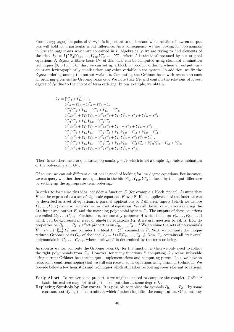
From a cryptographic point of view, it is important to understand what relations between outputbits will hold for a particular input difference. As a consequence, we are looking for polynomialsin just the output bits which are contained in I. Algebraically, we are trying to find elements ofthe ideal IY = I

⋂F2[Y ′1,0, . . . , Y

′1,3, Y

′′1,0, . . . , Y

′′1,3] where I is the ideal spanned by our original

equations. A deglex Grobner basis GY of this ideal can be computed using standard eliminationtechniques [3, p.168]. For this, we can set up a block or product ordering where all output vari-ables are lexicographically smaller than any other variable in the system. In addition, we fix thedeglex ordering among the output variables. Computing the Grobner basis with respect to suchan ordering gives us the Grobner basis GY . We note that GY will contain the relations of lowestdegree of IY due to the choice of term ordering. In our example, we obtain:

GY = [Y ′1,3 + Y ′′1,3 + 1,

Y ′1,0 + Y ′1,2 + Y ′′1,0 + Y ′′1,2 + 1,

Y ′′1,0Y′′1,2 + Y ′1,2 + Y ′′1,0 + Y ′′1,1 + Y ′′1,3,

Y ′′1,0Y′′1,1 + Y ′′1,0Y

′′1,3 + Y ′′1,1Y

′′1,2 + Y ′′1,2Y

′′1,3 + Y ′1,1 + Y ′′1,0 + Y ′′1,1,

Y ′1,2Y′′1,2 + Y ′′1,1Y

′′1,2 + Y ′′1,2Y

′′1,3,

Y ′1,2Y′′1,0 + Y ′′1,1Y

′′1,2 + Y ′′1,2Y

′′1,3 + Y ′1,1 + Y ′1,2 + Y ′′1,0 + Y ′′1,3,

Y ′1,1Y′′1,2 + Y ′1,2Y

′′1,1 + Y ′1,2Y

′′1,3 + Y ′′1,1Y

′′1,2 + Y ′1,1 + Y ′1,2 + Y ′′1,1,

Y ′1,1Y′′1,1 + Y ′1,1Y

′′1,3 + Y ′′1,1Y

′′1,2 + Y ′′1,1Y

′′1,3 + Y ′′1,2Y

′′1,3 + Y ′′1,1,

Y ′1,1Y′′1,0 + Y ′1,2Y

′′1,1 + Y ′1,2Y

′′1,3 + Y ′′1,0Y

′′1,3 + Y ′′1,1Y

′′1,2 + Y ′′1,2Y

′′1,3 + Y ′1,1 + Y ′′1,3,

Y ′1,1Y′1,2 + Y ′1,2Y

′′1,3 + Y ′′1,1Y

′′1,2 + Y ′′1,2Y

′′1,3 + Y ′1,2].

There is no other linear or quadratic polynomial p ∈ IY which is not a simple algebraic combinationof the polynomials in GY .

Of course, we can ask different questions instead of looking for low degree equations. For instance,we can query whether there are equations in the bits Y ′1,3, Y

′′1,2, Y

′′1,3 induced by the input difference

by setting up the appropriate term ordering.

In order to formalise this idea, consider a function E (for example a block cipher). Assume thatE can be expressed as a set of algebraic equations F over F. If one application of the function canbe described as a set of equations, d parallel applications to d different inputs (which we denoteP0, . . . , Pd−1) can also be described as a set of equations. We call the set of equations relating thei-th input and output Ei and the matching polynomial system Fi. The outputs of these equationsare called C0, . . . , Cd−1. Furthermore, assume any property Λ which holds on P0, . . . , Pd−1 andwhich can be expressed in a set of algebraic equations FΛ. A natural question to ask is: How doproperties on P0, . . . , Pd−1 affect properties on C0, . . . , Cd−1 ? We combine the sets of polynomials

F = FΛ ∪ (⋃d−1i=0 Fi) and consider the Ideal I = 〈F 〉 spanned by F . Next, we compute the unique

reduced Grobner basis GC of the ideal IC = I ∩ F[C0, . . . , Cd−1]. Now GC contains all “relevant”polynomials in C0, . . . , Cd−1, where “relevant” is determined by the term ordering.

As soon as we can compute the Grobner basis GC for the function E then we only need to collectthe right polynomials from GC . However, for many functions E computing GC seems infeasibleusing current Grobner basis techniques, implementations and computing power. Thus we have torelax some conditions hoping that we still can recover some equations using a similar technique. Weprovide below a few heuristics and techniques which still allow recovering some relevant equations.

Early Abort. To recover some properties we might not need to compute the complete Grobnerbasis, instead we may opt to stop the computation at some degree D.

Replacing Symbols by Constants. It is possible to replace the symbols P0, . . . , Pd−1 by someconstants satisfying the constraint Λ which further simplifies the computation. Of course any

40

polynomial recovered from such a computation would have to be checked against other valuesto verify that it actually holds in general or with high probability.

Choosing a Different Term Ordering. Instead of computing with respect to an eliminationordering, which is usually more expensive than a degree compatible ordering, we may choose toperform our computations with respect to an easier ordering such as degrevlex. Used togetherwith Early Abort, we have no assurances about the uniqueness and completeness of therecovered system. However, we might still be able to recover some information.

Computing Normal Forms Only. We can also compute equations by computing normal formsonly. For many ciphers it is possible to construct a Grobner basis for the round transformation[7, 8] with respect to some elimination ordering without any polynomial reductions. Theseconstructions exploit the fact that a system of polynomials is a Grobner basis if each polynomialhas a leading term which is pairwise prime with every other leading term. Using this property,we may construct a Grobner basis for some elimination ordering for the inverse of the cipher,i.e. the decryption process, such that the input variables are lexicographically bigger than theoutput variables of some round. Furthermore, we construct the term ordering such that thevariables of round i−1 are lexicographically bigger than the variables for round i. Furthermore,the symbols Ci are the lexicographically smallest.

If G′ is such a Grobner basis for r rounds for the first encryption and G′′ such a Grobner basisfor r rounds for the second encryption, we can combine these bases to G = G′ ∪G′′ which stillis a Grobner basis. Now we can compute the normal form of X ′i+X ′′i +∆Xi with respect to G.This will eliminate all variables > Ci as much as possible by construction. If this computationdoes not give equations in the Ci only, we may opt to perform an interreduction on severalsuch equations hoping that this way the remaining key bits are eliminated. For example, sucha Grobner basis for one application of the Present S-Box is

X1,0 + Y1,0Y1,1Y1,3 + Y1,1Y1,2Y1,3 + Y1,2Y1,3 + Y1,0 + Y1,1 + Y1,2 + Y1,3,

X1,1 + Y1,0Y1,1Y1,3 + Y1,0Y1,2Y1,3 + Y1,1Y1,2Y1,3 + Y1,0Y1,2 + Y1,0Y1,3

+ Y1,1Y1,2 + Y1,1Y1,3 + Y1,2Y1,3 + Y1,0 + 1,

X1,2 + Y1,0Y1,1Y1,3 + Y1,0Y1,2Y1,3 + Y1,1Y1,2Y1,3 + Y1,0Y1,1 + Y1,0Y1,2

+ Y1,1Y1,3 + Y1,0 + Y1,2 + Y1,3,

X1,3 + Y1,0Y1,2 + Y1,1 + Y1,3 + 1

The normal form of the equation X ′1,3 +X ′′1,3 + 1 with respect to G (i.e. two of such systemsfor X ′, Y ′ and X ′′, Y ′′) is Y ′1,0Y

′1,2 + Y ′′1,0Y

′′1,2 + Y ′1,1 + Y ′1,3 + Y ′′1,1 + Y ′′1,3 + 1.

4 Case Studies

To demonstrate our techniques, we consider the block ciphers Present and Ktantan32.

Present [5] was proposed at CHES 2007 as an ultra-lightweight block cipher, enabling a verycompact implementation in hardware, and therefore particularly suitable for RFIDs and similardevices. There are two variants of Present: one with 80-bit keys and one with a 128-bit keys,denoted as Present-80 and Present-128 respectively.

Present is an SP-network with a blocksize of 64 bits and both versions have 31 rounds. Each roundof the cipher has three layers of operations: keyAddLayer, sBoxLayer and pLayer. The operationkeyAddLayer is a simple subkey addition to the current state, while the sBoxLayer operationconsists of 16 parallel applications of a 4-bit S-Box. The operation pLayer is a permutation ofwires.

41

The Present authors give a security analysis of their cipher by showing resistance against well-known attacks such as differential and linear cryptanalysis [5]. The best published differentialattacks are for 16 rounds of Present-80 [27] and 17 (and possibly up to 19) rounds [1] forPresent-128. Results on linear cryptanalysis for up to 26 rounds are available in [10, 24]. Bit-pattern based integral attacks [28] are successful up to seven rounds of Present. A new type ofattack, called statistical saturation attack, was proposed in [14] and shown to be applicable up to24 rounds of Present.

KTANTAN32 [9] was proposed at CHES 2009 and is the smallest cipher in a family of blockciphers proposed in [9]. It allows a very compact implementation in hardware. It has a blocksizeof 32 bits and accepts an 80-bit key. The input is loaded into two registers L2 and L1 of 19 and13 bit length respectively. A round transformation is then applied to these registers 254 times.This round function updates two bits using a quadratic function and performs rotations on theregisters. After 254 rounds the content of L2 and L1 is outputed as the ciphertext.

The designers of KTANTAN consider a wide range of attacks in their security argument and showthe cipher secure against differential, linear, impossible differential, algebraic attacks and somecombined attacks. So far, there are no third-party security analyses of the cipher of which theauthors are aware.

5 Reducing the Noise

Recall that in order to discard wrong pairs, [1] proposed a technique referred to as Attack-C.In this context, the attacker considers an equation system modelling only the rounds > r. Theattacker is left with R rounds for each plaintext–ciphertext pair to consider. These are related bythe output difference predicted by the differential. If we denote the equation system for the lastR rounds of the encryption of P ′ to C ′ or P ′′ to C ′′ as F ′R or F ′′R respectively. The algebraic partof Attack-C is a Grobner basis computation on the polynomial system

F = F ′R ∪ F ′′R ∪ X ′r+1,i +X ′′r+1,i +∆Xr+1,i | 0 ≤ i < Bs.

Whenever the Grobner basis is equivalent to 1, we know that the analysed pair could not havebeen a right pair. Thus the pair can be discarded. However, no strong assurances are given in [1]as to how many pairs are actually discarded by this technique4.

In the this work, we consider the same system of equations as in Attack-C but replace the tuples ofconstants C ′ and C ′′ by tuples of symbols. By computing a Grobner basis for the right eliminationordering (cf. Section 3), we can recover equations in the variables C ′ and C ′′ which must evaluateto zero on the actual ciphertext values as soon as the input difference for round r+ 1 holds. Oncewe recovered such equations we can calculate the probability that all these polynomials evaluateto zero for random values for C ′ and C ′′. This gives an estimate about the quality of the filter.Furthermore, if the equations in C ′ and C ′′ are of sufficiently small degree, this filter is much fasterthan Attack-C since no Grobner basis has to be computed for each pair.

5.1 Case Study: PRESENT

We consider the differential from [27] and construct filters for Present reduced to 14 +R rounds.The same filter applies also to 10 +R, 6 +R and 2 +R rounds since the characteristic is iterativewith a period of four rounds. The explicit polynomials in this section do not differ for Present-80and Present-128.4 Note that Attack-B in [1] is guaranteed to distinguish right pairs eventually.

42

PRESENT 1R. We consider the polynomial ring P =

F2[ K0,0, . . . ,K0,79, K1,0, . . . ,K1,3,Y ′1,0, . . . , Y

′1,63, Y ′′1,0, . . . , Y

′′1,63, X ′1,0, . . . , X

′1,63, X ′′1,0, . . . , X

′′1,63,

. . . , K15,0, . . . ,K15,3,Y ′15,0, . . . , Y

′15,63, Y

′′15,0, . . . , Y

′′15,63, X

′15,0, . . . , X

′′15,63, X

′′15,0, . . . , X

′′15,63,

C ′0, . . . , C′63, C ′′0 , . . . , C

′′63]

and attach the following block ordering:

K0,0, . . . , X′′15,63︸︷︷︸

degrevlex

, C ′0, . . . , C′′63, C

′′0 , . . . , C

′′63︸︷︷︸

degrevlex

.

We set up an equation system as in Attack-C of [1], except that the ciphertext bits are symbols(C ′i and C ′′i ). Then, we compute the Grobner basis up to degree D = 3 using PolyBoRi 0.6.3 [6](as shipped with the Sage [26] mathematics software) with the option deg bound=3 and filter outany polynomial that contains non-ciphertext variables.

This computation returns 60 polynomials of which 58 are linear. These 58 linear polynomials areof the form C ′i + C ′′i for

i ∈ 0, . . . , 6, 8, . . . 14, 16, . . . 22, 24, . . . 30, 32, . . . 38, 40, . . . 46, 48, . . . , 63.

The remaining two polynomials are (C ′23 + C ′′23 + 1)(C ′7 + C ′39 + C ′′7 + C ′′39 + 1) and (C ′31 + C ′′31 +1)(C ′15 +C ′47 +C ′′15 +C ′′47 + 1). The probability that all polynomials evaluate to zero on a randompoint is approximately 2−58.83.

PRESENT 2R. We extend the ring and the system from the 1R experiment in the obviousway and perform the same computation as before. This computation returns 65 polynomials ofwhich 46 are linear. Forty linear polynomials are of the form C ′i +C ′′i and encode the informationthat the last round output difference of 10 S-Boxes must be zero (cf. [27]). The remaining 24polynomials split into two sets F0, F2 of 12 polynomials in 24 variables each and the Fj do notshare any variables with each other or the first 40 linear polynomials. The systems Fj are listedin Figure 2 in the Appendix. The probability that all polynomials evaluate to zero for a randompoint is ≈ 2−50.669.

For comparison, we construct random pairs C ′, C ′′ which pass this polynomial filter and noticethat for Attack-C from [1] roughly every second such pair for Present-80 and 317 out of 512for Present-128 will pass. Thus we expect Attack-C to pass with probability ≈ 2−51.669 forPresent-80 and with probability ≈ 2−51.361 for Present-128. Finally, we recall that Wang’sfilter from [27] passes with probability 2−40 · (5/16)6 ≈ 2−50.07.

PRESENT 3R. We extend the ring and the block ordering in the obvious way and computea Grobner basis with degree bound 3. The computation returns 28 polynomials of which 16 arelinear. The linear polynomials have the form C ′i + C ′′i for

i ∈ 3, 7, 11, 15, 19, 23, 27, 31, 35, 39, 43, 47, 51, 55, 59, 63.

The remaining 12 polynomials are quadratic and cubic (cf. Figure 3 in the Appendix). The prob-ability that all polynomials evaluate to zero on a random point is ≈ 2−18.296. To compare withAttack-C, we construct random pairs C ′, C ′′ which pass this polynomial filter. Attack-C will acceptroughly 6 in 1024 pairs for Present-80 and 9 out of 1024 pairs for Present-128. Thus, we expectAttack-C to pass with probability ≈ 2−25.711 for Present-80 and 2−25.126 for Present-128.

43

PRESENT 4R. We extend the ring and the block ordering in the obvious way. With a degreebound D = 3 we recover

(C ′32+j + C ′′32+j + 1)(C ′j + C ′′j + 1)(C ′16+j + C ′48+j + C ′′16+j + C ′′48+j)

for 0 ≤ j < 16. The probability that all polynomials evaluate to zero on a random point is≈ 2−3.082. We verified experimentally that this bound is optimal by using the SAT solver Cryp-toMiniSat [25] on Attack-C systems in a 4R attack against Present-80-14. The solver returnedan assignment which satisfies the equation system with probability ≈ 2−3. Thus, we conclude thatAttack-C will roughly accept 1 in 8 pairs.

5.2 Case Study: KTANTAN

In Table 1 we give our results against Ktantan32. We used the best differential for 42 roundsas provided by the KTANTAN designers and extended it to 71 rounds. The characteristic has aprobability of 2−31. Below we present results for the degree bounded at four and at five respectively.For each degree bounds we give the number of degree 1-5 polynomials (denoted as d = ∗) we found.In the last column of each experiment we give the approximate probability that all the equationswe found evaluate to zero for random values (denoted log2 p).

degree bound = 4 degree bound = 5

N d = 1 d = 2 d = 3 d = 4 d = 5 log2 p d = 1 d = 2 d = 3 d = 4 d = 5 log2 p

72 32 0 0 0 0 −32.0 32 0 0 0 0 −32.074 32 0 0 0 0 −32.0 32 0 0 0 0 −32.076 32 0 0 0 0 −32.0 32 0 0 0 0 −32.078 31 3 0 0 0 −32.0 31 3 0 0 0 −32.080 28 11 0 0 0 −31.4 28 11 0 0 0 −31.482 25 23 0 0 0 −31.0 25 23 0 0 0 −31.084 20 32 4 8 0 −29.0 20 32 4 32 0 −29.086 16 44 19 8 0 −25.7 16 46 23 75 106 < −2488 12 39 54 96 0 −24.0 12 51 103 371 745 < −2390 8 41 129 287 0 −23.0 8 42 133 612 1762 < −2292 4 28 113 285 0 −20.0 4 33 133 743 2646 −20.494 1 20 94 244 0 −16.3 1 25 124 662 2345 −18.596 0 8 38 96 0 −12.8 0 8 52 287 1264 −14.398 0 3 8 29 0 −7.0 0 3 10 46 156 −9.1100 0 1 3 13 0 −3.7 0 1 3 18 47 −4.6102 0 0 0 2 0 −0.8 0 0 0 4 9 −0.9103 0 0 0 1 0 −0.4 0 0 0 2 4 −0.4104 0 0 0 0 0 0.0 N/A N/A N/A N/A N/A N/A

Table 1. Decreasing the noise for Ktantan32.

6 Increasing the Signal

In this section, we consider the problem of increasing the amount of correct data that has toagree and is always suggested by a right pair. Increasing this value usually has considerable costsattached to it. First, more data needs to be managed and thus usually the counter tables get bigger.On average, we can expect each additional bit considered to double the size of these tables. Second,

44

in order to generate more data, more partial decryptions must be performed which increases thecomputation time. Additionally, the number of key bits that can be trial decrypted might belimited by the number of rounds R we can consider because of the quality of the filter.

In this work we use (non-linear) data available from the first few rounds instead of the last Rrounds. Assume that we have an SP-network, a differential characteristic ∆ = (∆P,∆Y1, . . . ,∆Yr)valid for r rounds with probability p, and (P ′, P ′′) a right pair for ∆ (so that ∆P = P ′ ⊕ P ′′ and∆Yr holds for the output of round r). For simplicity, let us assume that only one S-Box is activein round 1, with input X ′1,j and X ′′1,j (restricted to this S-Box) for the plaintext P ′ and P ′′

respectively, and that there is a key addition immediately before the S-Box operation, that is

S(P ′j ⊕K0,j) = S(X ′1,j) = Y ′1,j and S(P ′′j ⊕K0,j) = S(X ′′1,j) = Y ′′1,j .

The S-Box operation S can be described by a (vectorial) Boolean function, expressing each bit ofthe output Y ′1,j as a polynomial function (over F2) on the input bits of X ′1,j and K0,j . If (P ′, P ′′)is a right pair, then the polynomial equations arising from the relation ∆Y1,j = Y ′1,j ⊕ Y ′′1,j =S(P ′j ⊕ K0,j) ⊕ S(P ′′j ⊕ K0,j) gives us a very simple equation system to solve, with only thekey variables K0,j as unknowns (and which do not vanish identically because we are consideringnonzero differences). Consequently, right pairs suggest additional information about the key fromthe first round difference. In particular, if ∆Y1 holds with probability 2−b then we can recover bbits of information about the key, if we found a right pair.

There is no a priori reason to restrict this argument from [1] to the first round. Let ∆, r, P ′, P ′′

be as before. We setup two equation systems F ′ and F ′′ involving P ′, C ′ and P ′′, C ′′ respectivelyand discard any polynomials from the rounds > s where s is a small integer > 0. Previously wehad s = 1. Finally, we add linear equations as suggested by the characteristic and use this systemto recover information about the key from the first s rounds.

In order to avoid the potentially costly Grobner basis computation for every candidate pair replacethe tuples of constants P ′ and P ′′ by tuples of symbols. According to Section 3, we can computepolynomials involving only key variables and the newly introduced plaintext variables P ′ and P ′′.Assume that we can indeed compute the Grobner basis with P ′ and P ′′ symbols for the first srounds and the linear equations arising from the characteristic added. Assume further that theprobability that the characteristic restricted to s rounds holds is 2−b and that we computed ms

polynomials in the variables K0, P ′ and P ′′. This means that we recover b bits of informationwhen we evaluate all ms polynomials such that we replace P ′ and P ′′ by their actual values.

This means that we have b bits of extra information and thus can write S/N = 2k+b·pα·β without

the overhead of performing any partial decryptions. However, we have to perform ms polynomialevaluations (where we replace P ′ and P ′′ by their actual values) of relatively small low degreepolynomials.

Case Study: PRESENT. We consider the first two encryption rounds and the characteristicfrom [27]. We set up a polynomial ring with two blocks such that the variables Pi and Ki are lexi-cographically smaller than any other variables. Within the blocks we chose a degree lexicographicalterm ordering. We set up an equation system covering the first two encryption rounds and addedthe linear equations suggested by the characteristic. Then, we eliminated all linear leading termswhich are not in the variables Pi and Ki and computed a Grobner basis up to degree five. Thiscomputation returned 22 linear and quadratic polynomials (we give the Grobner basis for thesepolynomials in Figure 4). This system gives 8 bits of information about the key. Note that thefirst two rounds of the characteristic pass with probability 2−8.

45

Case Study: KTANTAN32. We consider the first 24 rounds of KTANTAN32 and computethe full Grobner basis. This computation recovers 39 polynomials. We list an excerpt in Figure 1in the Appendix. As expected we observe that the characteristic also imposes restrictions on theplaintext. These eight equations allow us to recover up to four bits (depending on the value ofP ′19) of information about the key.

Acknowledgements

We would like to thank William Stein for allowing us to run our experiments on his computers5.We would also like to thank anonymous referees for helpful comments.

Conclusion

In this work, we have introduced a novel application for the algebraic cryptanalysis of block ci-phers. We propose a method which can improve “classical” differential cryptanalysis, by applyingalgebraic tools in a pre-computation phase. As such, we shift the focus from attempting to solvelarge systems of polynomial equations to recovering symbolic information about the underlyingcipher. Although the use of algebraic techniques in general, and Grobner basis methods in particu-lar, in block cipher cryptanalysis has received some criticism within the cryptographic community,as it has been often the case that “simpler” techniques can perform favourably in many situations,we stress that the rich algebraic structure of Grobner basis can offer many advantages and maygive one a more subtle insight of the cipher structure. This can in turn be used in the cryptanalysisof the cipher. We note that in principle our techniques can recover an optimal amount of infor-mation and that in almost all cases considered in this work we were (almost) able to accomplishthis. We expect that this approach is applicable to other cryptanalytical techniques such as linearand higher-order differential cryptanalysis and consider applying it as an area of future work.

References

1. Martin Albrecht and Carlos Cid. Algebraic Techniques in Differential Cryptanalysis. In Fast SoftwareEncryption 2009, Lecture Notes in Computer Science, Berlin, Heidelberg, New York, 2009. SpringerVerlag.

2. Gwenole Ars. Applications des bases de Grobner a la cryptographie. PhD thesis, Universite de RennesI, 2005.

3. Thomas Becker and Volker Weispfenning. Grobner Bases - A Computational Approach to Commuta-tive Algebra. Springer Verlag, Berlin, Heidelberg, New York, 1991.

4. Eli Biham and Adi Shamir. Differential Cryptanalysis of DES-like Cryptosystems. In Advances inCryptology — CRYPTO 1990, volume 537 of Lecture Notes in Computer Science, pages 3–72, Berlin,Heidelberg, New York, 1991. Springer Verlag.

5. Andrey Bogdanov, Lars R. Knudsen, Gregor Leander, Christof Paar, Axel Poschmann, Matthew J. B.Robshaw, Yannick Seurin, and C. Vikkelsoe. PRESENT: An ultra-lightweight block cipher. In Crypto-graphic Hardware and Embedded Systems - CHES 2007, volume 7427 of Lecture Notes in Computer Sci-ence, pages 450–466, Berlin, Heidelberg, New York, 2007. Springer Verlag. Available at http://www.

crypto.rub.de/imperia/md/content/texte/publications/conferences/present_ches2007.pdf.

6. Michael Brickenstein and Alexander Dreyer. PolyBoRi: A framework for Grobner basis computationswith Boolean polynomials. In Electronic Proceedings of MEGA 2007, 2007. Available at http:

//www.ricam.oeaw.ac.at/mega2007/electronic/26.pdf.

5 Purchased under National Science Foundation Grant No. DMS-0821725.

46

7. Johannes Buchmann, Andrei Pychkine, and Ralf-Philipp Weinmann. A Zero-dimensional GrobnerBasis for AES-128. In Fast Software Encryption 2006, volume 4047 of Lecture Notes in ComputerScience, pages 78–88. Springer Verlag, 2006.

8. Stanislav Bulygin and Michael Brickenstein. Obtaining and solving systems of equations in keyvariables only for the small variants of AES. Mathematics in Computer Science, 2008. conditionallyaccepted for special issue ”Symbolic Computation and Cryptography”.

9. Christophe De Canniere, Orr Dunkelman, and Miroslav Knezevic. KATAN and KTANTAN — afamily of small and efficient hardware-oriented block ciphers. In Christophe Clavier and Kris Gaj,editors, Cryptographic Hardware and Embedded Systems - CHES 2009, volume 5747 of Lecture Notesin Computer Science, pages 272–288. Springer Verlag, 2009.

10. Joo Yeon Cho. Linear cryptanalysis of reduced-round PRESENT. Cryptology ePrint Archive, Report2009/397, 2009. available at http://eprint.iacr.org/2009/397.

11. Carlos Cid. D.STVL.7 algebraic cryptanalysis of symmetric primitives, 2008. available at http:

//www.ecrypt.eu.org/ecrypt1/documents/D.STVL.7.pdf.

12. Carlos Cid and Gaetan Leurent. An Analysis of the XSL Algorithm. In Advances in Cryptology— ASIACRYPT 2005, volume 3788 of Lecture Notes in Computer Science, pages 333–352, Berlin,Heidelberg, New York, 2005. Springer Verlag.

13. Carlos Cid, Sean Murphy, and Matthew Robshaw. Small Scale Variants of the AES. In Fast Soft-ware Encryption 2005, volume 3557 of Lecture Notes in Computer Science, pages 145–162, Berlin,Heidelberg, New York, 2005. Springer Verlag. Available at http://www.isg.rhul.ac.uk/~sean/

smallAES-fse05.pdf.

14. Baudoin Collard and Francois-Xavier Standaert. A Statistical Saturation Attack against the BlockCipher PRESENT. In Topics in Cryptology – CT-RSA 2009, pages 195–210, 2009.

15. Nicolas T. Courtois. Fast algebraic attacks on stream ciphers with linear feedback. In Advances inCryptology – CRYPTO 2003, volume 2729 of Lecture Notes in Computer Science, pages 176–194,2003.

16. Nicolas T. Courtois. Higher order correlation attacks, XL algorithm and cryptanalysis of Toyocrypt. InP.J. Lee and C.H. Lim, editors, Information Security and Cryptology - ICISC 2002: 5th InternationalConference, volume 2587 of Lecture Notes in Computer Science, Berlin, Heidelberg, New York, 2003.Springer Verlag.

17. Nicolas T. Courtois and Gregory V. Bard. Algebraic Cryptanalysis of the Data Encryption Standard.In Steven D. Galbraith, editor, Cryptography and Coding – 11th IMA International Conference, volume4887 of Lecture Notes in Computer Science, pages 152–169, Berlin, Heidelberg, New York, 2007.Springer Verlag. pre-print available at http://eprint.iacr.org/2006/402.

18. Nicolas T. Courtois and Willi Meier. Algebraic attacks on stream ciphers with linear feedback. InEli Biham, editor, Advances in Cryptology — EUROCRYPT 2003, volume 2656 of Lecture Notes inComputer Science, pages 345–359, Berlin, Heidelberg, New York, 2003. Springer Verlag.

19. Nicolas T. Courtois and Josef Pieprzyk. Cryptanalysis of block ciphers with overdefined systems ofequations. In Yuliang Zheng, editor, Advances in Cryptology — ASIACRYPT 2002, volume 2501of Lecture Notes in Computer Science, pages 267–287, Berlin, Heidelberg, New York, 2002. SpringerVerlag.

20. Jean-Charles Faugere, Francoise Levy dit Vehel, and Ludovic Perret. Cryptanalysis of MinRank. InAdvances in Cryptology – CRYPTO 2008, volume 5157 of Lecture Notes in Computer Science, pages280–296, 2008.

21. Jean-Charles Faugere and Antoine Joux. Algebraic cryptanalysis of hidden field equation (hfe) cryp-tosystems using grobner bases. In CRYPTO, pages 44–60, 2003.

22. Jean-Charles Faugere and Ludovic Perret. Cryptanalysis of 2r− schemes. In Advances in Cryptology– CRYPTO 2006, volume 4117 of Lecture Notes in Computer Science, pages 357–372, 2006.

23. Jean-Charles Faugere and Ludovic Perret. Polynomial equivalence problems: Algorithmic and theo-retical aspects. In Advances in Cryptology – EUROCRYPT 2006, volume 4004 of Lecture Notes inComputer Science, pages 30–47, 2006.

24. Jorge Nakahara Jr, Pouyan Seperhdad, Bingsheng Zhang, and Meiqin Wang. Linear (hull) and alge-braic cryptanalysis of the block cipher PRESENT. In The 8th International Conference on Cryptoplogyand Network Security - CANS 2009, 2009.

25. Mate Soos, Karsten Nohl, and Claude Castelluccia. Extending SAT solvers to cryptographic problems.In Oliver Kullmann, editor, Theory and Applications of Satisfiability Testing - SAT 2009, volume 5584of Lecture Notes in Computer Science, pages 244–257, Berlin, Heidelberg, New York, 2009. SpringerVerlag.

47

26. William Stein et al. SAGE Mathematics Software. The Sage Development Team, 2008. Available athttp://www.sagemath.org.

27. Meiqin Wang. Differential Cryptanalysis of reduced-round PRESENT. In Serge Vaudenay, editor,Africacrypt 2008, volume 5023 of Lecture Notes in Computer Science, pages 40–49, Berlin, Heidelberg,New York, 2008. Springer Verlag.

28. Muhammad Reza Z’Aba, Havard Raddum, Matt Henricksen, and Ed Dawson. Bit-pattern basedintegral attacks. In Kaisa Nyberg, editor, Fast Software Encryption 2008, number 5086 in LectureNotes In Computer Science, pages 363–381, Berlin, Heidelberg, New York, 2008. Springer Verlag.

48

A Explicit Polynomials

(P ′19 + 1)(P ′3P′8 + P ′10P

′12 +K3 +K53 + P ′7 + P ′18 + P ′23),

P ′8P′10P

′19 +K8P

′19 + P ′3P

′8 + P ′6P

′19 + P ′10P

′12

+P ′16P′19 +K3 +K53 + P ′7 + P ′18 + P ′19 + P ′23,

P ′19P′22 +K1 +K11 + P ′6 + P ′11 + P ′17 + P ′21 + P ′26,

P ′23P′26 +K65 + P ′21 + P ′25 + P ′30,

P ′1 + 1, P ′2, P′5 + 1, P ′9 + 1

Fig. 1. Polynomials for the first two rounds of Ktantan32.

(C′57+j + C′′57+j)(C′53+j + C′′53+j + 1)(C′17+j + C′′17+j),

(C′57+j + C′′57+j)(C′53+j + C′′53+j + 1)(C′33+j + C′′33+j),

(C′57+j + C′′57+j + 1)(C′25+j + C′′25+j),

(C′57+j + C′′57+j + 1)(C′41+j + C′′41+j),

(C′53+j + C′′53+j + 1)(C′21+j + C′′21+j),

(C′53+j + C′′53+j + 1)(C′37+j + C′′37+j),

(C′53+j + C′′53+j + 1)(C′49+j + C′57+j + C′′49+j + C′′57+j + 1),

(C′49+j + C′′49+j + 1)(C′17+j + C′′17+j),

(C′49+j + C′′49+j + 1)(C′33+j + C′′33+j),

C′1+j + C′33+j + C′49+j + C′′1+j + C′′33+j + C′′49+j ,

C′5+j + C′37+j + C′53+j + C′′5+j + C′′37+j + C′′53+j ,

C′9+j + C′41+j + C′57+j + C′′9+j + C′′41+j + C′′57+j ,

Fig. 2. 2R polynomials for Present with j ∈ 0, 2.

49

(C′36 + C′′36)((C′4 + C′′4 )(C′20 + C′52 + C′′20 + C′′52 + 1) + (C′20 + C′′20 + 1)(C′52 + C′′52 + 1)),

(C′37 + C′′37)((C′5 + C′′5 )(C′21 + C′53 + C′′21 + C′′53 + 1) + (C′21 + C′′21 + 1)(C′53 + C′′53 + 1)),

(C′40 + C′′40)((C′8 + C′′8 )(C′24 + C′56 + C′′24 + C′′56 + 1) + (C′24 + C′′24 + 1)(C′56 + C′′56 + 1)),

(C′41 + C′′41)((C′9 + C′′9 )(C′25 + C′57 + C′′25 + C′′57 + 1) + (C′25 + C′′25 + 1)(C′57 + C′′57 + 1)),

(C′45 + C′′45)((C′13 + C′′13)(C′29 + C′61 + C′′29 + C′′61 + 1) + (C′29 + C′′29 + 1)(C′61 + C′′61 + 1)),

(C′46 + C′′46)((C′14 + C′′14)(C′30 + C′62 + C′′30 + C′′62 + 1) + (C′30 + C′′30 + 1)(C′62 + C′′62 + 1)),

(C′06 + C′′06)((C′22 + C′′22)(C′38 + C′54 + C′′38 + C′′54 + 1) + (C′38 + C′′38 + 1)(C′54 + C′′54 + 1)),

(C′10 + C′′10)((C′26 + C′′26)(C′42 + C′58 + C′′42 + C′′58 + 1) + (C′42 + C′′42 + 1)(C′58 + C′′58 + 1)),

(C′12 + C′′12)((C′28 + C′′28)(C′44 + C′60 + C′′44 + C′′60 + 1) + (C′44 + C′′44 + 1)(C′60 + C′′60 + 1)),

(C′52 + C′′52 + 1)(C′20 + C′′20 + 1)(C′4 + C′36 + C′′4 + C′′36),

(C′60 + C′′60 + 1)(C′28 + C′′28 + 1)(C′12 + C′44 + C′′12 + C′′44),

(C′10 + C′42 + C′58 + C′′10 + C′′42 + C′′58)(C′2 + C′34 + C′50 + C′′2 + C′′34 + C′′50).

Fig. 3. 3R polynomials for Present.

(K1 + P ′1 + 1)(K0 +K3 +K29 + P ′0 + P ′3),

(K2 + P ′2)(K0 +K3 +K29 + P ′0 + P ′3),

K1K2 +K1P′2 +K2P

′1 + P ′1P

′2 +K0 +K1 +K3 +K29 + P ′0 + P ′1 + P ′3,

(K9 + P ′9 + 1)(K8 +K11 +K31 + P ′8 + P ′11),

(K10 + P ′10)(K8 +K11 +K31 + P ′8 + P ′11),

K9K10 +K9P′10 +K10P

′9 + P ′9P

′10 +K8 +K9 +K11 +K31 + P ′8 + P ′9 + P ′11,

(K49 + P ′49 + 1)(K41 +K48 +K51 + P ′48 + P ′51),

(K50 + P ′50)(K41 +K48 +K51 + P ′48 + P ′51),

K49K50 +K49P′50 +K50P

′49 + P ′49P

′50 +K41 +K48 +K49 +K51 + P ′48 + P ′49 + P ′51,

(K57 + P ′57 + 1)(K43 +K56 +K59 + P ′56 + P ′59),

(K58 + P ′58)(K43 +K56 +K59 + P ′56 + P ′59),

K57K58 +K57P′58 +K58P

′57 + P ′57P

′58 +K43 +K56 +K57 +K59 + P ′56 + P ′57 + P ′59,

K5 +K7 + P ′5 + P ′7,

K6 +K7 + P ′6 + P ′7,

K53 +K55 + P ′53 + P ′55,

K54 +K55 + P ′54 + P ′55

Fig. 4. Polynomials for the first two rounds of Present.

50

SYMAES: A Fully Symbolic Polynomial SystemGenerator for AES-128⋆

Vesselin Velichkov1,2,⋆⋆, Vincent Rijmen1,2,3, and Bart Preneel1,2

1 Department of Electrical Engineering ESAT/SCD-COSIC,Katholieke Universiteit Leuven. Kasteelpark Arenberg 10, B-3001 Heverlee, Belgium.

[email protected] Interdisciplinary Institute for BroadBand Technology (IBBT), Belgium.

3 Graz University of Technology.

SYMAES is a software tool that generates a system of polynomials in GF(2),corresponding to the round transformation and key schedule of the block cipherAES-128 [1].

Most of the existing polynomial system generators for AES are typically usedunder the assumption that the plaintext and ciphertext bits are known, and there-fore are treated as constants. Although some of the generators, such as the AES(SR) Polynomial System Generator [2,3], can also be used when this assumptionis not made, the instructions to do this are not always very natural. SYMAESis specifically designed to address the case in which (some of) the plaintext andciphertext bits are unknown and are therefore treated as symbolic variables. Sucha scenario is realistic and arises during the algebraic cryptanalysis of AES-basedconstructions, where only parts of the plaintext and/or ciphertext are known. Anexample of such a construction is the stream cipher LEX [4], a small-scale versionof which has been analysed using SYMAES [5].

The inputs to SYMAES are the bits of the plaintext and the bits of the orig-inal key, represented as symbolic variables in GF(2). The output is a system ofequations describing the output bits of one round of AES as a function of theinput bits and the key. SYMAES also generates symbolic equations for the AESkey schedule. Then, the bits of the round keys are expressed as polynomials in thebits of the original key.

As a final note we would like to stress that SYMAES should not be seen asa competitor to existing AES polynomial system generators, but rather as anaddition to them. SYMAES achieves in a more natural way what can also beachieved using SR [3]. Similarly to SR, SYMAES is also written in Python andis used within the open source computer algebra Sage [6]. This makes possible afuture integration of the SYMAES code into SR.

This submission is accompanied by an appendix containing the SYMAESsource code and usage instructions.

References

1. Joan Daemen, Vincent Rijmen, The Design of Rijndael: AES - The Advanced En-cryption Standard, Springer-Verlag, 2002.

2. Carlos Cid, Sean Murphy, Matthew J. B. Robshaw: Small Scale Variants of the AES.FSE 2005: 145-162.

⋆ This work was supported in part by the IAP Program P6/26 BCRYPT of the BelgianState (Belgian Science Policy), and in part by the European Commission through theICT program under contract ICT-2007-216676 ECRYPT II.

⋆⋆ DBOF Doctoral Fellow, K.U.Leuven, Belgium.

51

3. Martin Albrecht, Small Scale Variants of the AES (SR) Polynomial System Gener-ator, available at http://www.sagemath.org/doc/reference/sage/crypto/mq/sr.

htm.4. Alex Biryukov, The Design of a Stream Cipher Lex. Selected Areas in Cryptography

2006:67-75.5. V. Velichkov, V. Rijmen, and B. Preneel, Algebraic Cryptanalysis of a Small-Scale

Version of Stream Cipher LEX, IET Information Security Journal, 16 pages, 2009,to appear.

6. Stein, William, Sage: Open Source Mathematical Software (Version 3.1.4), TheSage Group, 2008, http://www.sagemath.org.

2

52

Efficient Decomposition of Dense Matrices over GF(2)

Martin R. Albrecht?1 and Clement Pernet2

1 Information Security Group, Royal Holloway, University of LondonEgham, Surrey TW20 0EX, United Kingdom

[email protected] INRIA-MOAIS LIG, Grenoble Univ. ENSIMAG, Antenne de Montbonnot 51,avenue Jean Kuntzmann, F-38330 MONTBONNOT SAINT MARTIN, France

[email protected]

Abstract. In this work we describe an efficient implementation of a hierarchy ofalgorithms for the decomposition of dense matrices over the field with two elements(F2). Matrix decomposition is an essential building block for solving dense systemsof linear and non-linear equations and thus much research has been devoted toimprove the asymptotic complexity of such algorithms. In this work we discuss animplementation of both well-known and improved algorithms in the M4RI library.The focus of our discussion is on a new variant of the M4RI algorithm – denotedMMPF in this work – which allows for considerable performance gains in practicewhen compared to the previously fastest implementation. We provide performancefigures on x86 64 CPUs to demonstrate the viability of our approach.

1 Introduction

We describe an efficient implementation of a hierarchy of algorithms for PLS decompo-sition of dense matrices over the field with two elements (F2). The PLS decompositionis closely related to the well-known PLUQ and LQUP decompositions. However, it of-fers some advantages in the particular case of F2. Matrix decomposition is an essentialbuilding block for solving dense systems of linear and non-linear equations (cf. [11, 10])and thus much research has been devoted to improve the asymptotic complexity of suchalgorithms. In particular, it has been shown that various matrix decompositions such asPLUQ, LQUP and LPS are essentially equivalent and can be reduced to matrix-matrixmultiplication (cf. [13]). Thus, we know that these decompositions can be achieved inO(nω) where ω is the exponent of linear algebra3. In this work we focus on matrix de-composition in the special case of F2 and discuss an implementation of both well-knownand improved algorithms in the M4RI library [2]. The M4RI library implements denselinear algebra over F2 and is used by the Sage [16] mathematics software and the Poly-BoRi [9] package for computing Grobner bases. It is also the linear algebra library usedin [15, 14].

Our implementation focuses on 64-bit x86 architectures (x86 64), specifically the IntelCore 2 and the AMD Opteron. Thus, we assume in this chapter that each native CPUword has 64 bits. However it should be noted that our code also runs on 32-bit CPUs andon non-x86 CPUs such as the PowerPC.

? This author was supported by the Royal Holloway Valerie Myerscough Scholarship.3 For practical purposes we set ω = 2.807.

53

Element-wise operations over F2 are relatively cheap compared to loads from andwrites to memory. In fact, in this work we demonstrate that the two fastest implemen-tations for dense matrix decomposition over F2 (the one presented in this work and theone found in Magma [8] due to Allan Steel) perform worse for sparse matrices despitethe fact that fewer field operations are performed. This indicates that counting raw fieldoperations is not an adequate model for estimating the running time in the case of F2.

This work is organised as follows. We will start by giving the definitions of reduced rowechelon forms (RREF), PLUQ and PLS decomposition in Section 2 and establish theirrelations. We will then discuss Gaussian elimination and the M4RI algorithm in Section 3followed by a discussion of cubic PLS decomposition and the MMPF algorithm in 4. Wewill then discuss asymptotically fast PLS decomposition in Section 5 and implementationissues in Section 6. We conclude by giving empirical evidence of the viability of ourapproach in Section 7.

2 RREF and PLS

Proposition 1 (PLUQ decomposition). Any m×n matrix A with rank r, can be writ-ten A = PLUQ where P and Q are two permutation matrices, of dimension respectivelym×m and n× n, L is m× r unit lower triangular and U is r × n upper triangular.

Proof. See [13].

Proposition 2 (PLS decomposition). Any m×n matrix A with rank r, can be writtenA = PLS where P is a permutation matrix of dimension m×m, L is m× r unit lowertriangular and S is an r× n matrix which is upper triangular except that its columns arepermuted, that is S = UQ for U r × n upper triangular and Q is a n × n permutationmatrix.

Proof. Write A = PLUQ and set S = UQ.

Another way of looking at PLS decomposition is to consider the A = LQUP de-composition [12]. We have A = LQUP = LSP where S = QU . We can also writeA = LQUP = SUP where S = LQ. Applied to AT we then get A = PTUTST = P ′L′S′.Finally, a proof for Proposition 2 can also be obtained by studying any one of the Algo-rithms 9, 3 or 4.

Definition 1 (Row Echelon Form). An m × n matrix A is in echelon form if allzero rows are grouped together at the last row positions of the matrix, and if the leadingcoefficient of each non zero row is one and is located to the right of the leading coefficientof the above row.

Proposition 3. Any m×n matrix can be transformed into echelon form by matrix mul-tiplication.

Proof. See [13]

Note that while there are many PLUQ decompositions of any matrix A there is alwaysalso a decomposition for which we have that S = UQT is a row echelon form of A. In

54

this work we compute A = PLS such that S is in row echelon form. Thus, a proof forProposition 3 can also be obtained by studying any one of the Algorithms 9, 3 or 4.

Definition 2 (Reduced Row Echelon Form). An m × n matrix A is in reducedechelon form if it is in echelon form and each leading coefficient of a non zero row is theonly non zero element in its column.

3 Gaussian Elimination and M4RI

Gaussian elimination is the classical, cubic algorithm for transforming a matrix into (re-duced) row echelon form using elementary row operations only. The “Method of theFour Russians” Inversion (M4RI) [7] reduces the number of additions required by Gaus-sian elimination by a factor of log n by using a caching technique inspired by Kronrod’smethod for matrix-matrix multiplication.

3.1 The “Method of the Four Russians” Inversion (M4RI)

The “Method of the Four Russians” inversion was introduced in [5] and later describedin [6] and [7]. It inherits its name and main idea from the misnamed “Method of the FourRussians” multiplication [4, 1].

To give the main idea consider for example the matrix A of dimension m × n inFigure 3.1. The k × n (k = 3) submatrix on the top has full rank and we performedGaussian elimination on it. Now, we need to clear the first k columns of A for the rowsbelow k (and above the submatrix in general if we want the reduced row echelon form).There are 2k possible linear combinations of the first k rows, which we store in a table T .We index T by the first k bits (e.g., 011→ 3). Now to clear k columns of row i we use thefirst k bits of that row as an index in T and add the matching row of T to row i, causinga cancellation of k entries. Instead of up to k additions this only costs one addition due tothe pre-computation. Using Gray codes (or similar techniques) this pre-computation canbe performed in 2k vector additions and the overall cost is 2k+m−k+k2 vector additionsin the worst case (where k2 accounts for the Gauss elimination of the k × n submatrix).The naive approach would cost k ·m row additions in the worst case to clear k columns.If we set k = logm then the complexity of clearing k columns is O

(m+ log2m

)vector

additions in contrast to O(m · logm) vector additions using the naive approach.This idea leads to Algorithm 1. In this algorithm the subroutine GaussSubmatrix

(cf. Algorithm 8) performs Gauss elimination on a k × n submatrix of A starting atposition (r, c) and searches for pivot rows up to m. If it cannot find a submatrix of rankk it will terminate and return the rank k found so far. Note the technicality that theroutine GaussSubmatrix and its interaction with Algorithm 1 make use of the fact thatall the entries in a column below a pivot are zero if they were considered already.

The subroutine MakeTable (cf. Algorithm 7) constructs the table T of all 2k linearcombinations of the k rows starting a row r and a column c, i.e. it enumerates all elementsof the vector space span(r, ..., r+ k+ 1) spanned by the rows r, . . . , r+ k− 1. Finally, thesubroutine AddRowsFromTable (cf. Algorithm 6) adds the appropriate row from T –indexed by k bits starting at column c – to each row of A with index i 6∈ r, . . . , r+k−1.That is, it adds the appropriate linear combination of the rows r, . . . , r + k − 1 onto arow i in order to clear k columns.

55

A =

1 0 0 1 0 1 1 1 . . .0 1 0 1 1 1 1 0 . . .0 0 1 0 0 1 1 1 . . .

. . .0 0 0 1 1 0 1 0 . . .1 1 0 0 1 0 1 1 . . .0 1 0 0 1 0 0 1 . . .

. . .1 1 0 1 1 1 0 1 . . .

T =

0 0 0 0 0 0 0 0 . . .0 0 1 0 0 1 1 1 . . .0 1 0 1 1 1 1 0 . . .0 1 1 1 1 0 0 1 . . .1 0 0 1 0 1 1 1 . . .1 0 1 1 0 0 0 0 . . .1 1 0 0 1 0 0 1 . . .1 1 1 0 1 1 1 0 . . .

Fig. 1. M4RI Idea

Note that the relation between the index id and the row j in T is static and knowna priori because GaussSubmatrix puts the submatrix in reduced row echelon form. Inparticular this means that the k × k submatrix starting at (r, c) is the identity matrix.

Input: A – a m× n matrixInput: k – an integer k > 0Result: A is in reduced row echelon form.begin

r, c←− 0, 0;while c < n do

if c+ k > n then k ← n− c;k ←− GaussSubmatrix(A, r, c, k,m);if k > 0 then

T,L←− MakeTable(A, r, c, k);AddRowsFromTable(A, 0, r, c, k, T, L);AddRowsFromTable(A, r + k,m, c, k, T, L);

end

r, c←− r + k, c+ k;if k 6= k then c← c+ 1;

endend

Algorithm 1: M4RI

When studying the performance of Algorithm 1, we expect the function MakeTable

to contribute most. Instead of performing k/2·2k−1 additions MakeTable only performs

2k − 1 vector additions. However, in practice the fact that k columns are processed ineach loop iteration of AddRowsFromTable contributes signficiantly due to the bettercache locality. Assume the input matrix A does not fit into L2 cache. Gaussian eliminationwould load a row from memory, clear one column and likely evict that row from cache inorder to make room for the next few rows before considering it again for the next column.In the M4RI algorithm more columns are cleared per load.

We note that our presentation of M4RI differs somewhat from that in [6]. The keydifference is that our variant does not throw an error if it cannot find a pivot within

56

the first 3k rows in GaussSubmatrix. Instead, our variant searches all rows and conse-quently the worst-case complexity is cubic. However, on average for random matrices weexpect to find a pivot within 3k rows and thus expect the average-case complexity to beO(n3/ log n

).

4 M4RI and PLS Decomposition

In order to recover the PLS decomposition of some matrix A, we can adapt Gaussianelimination to preserve the transformation matrix in the lower triangular part of theinput matrix A and to record all permutations performed. This leads to Algorithm 9 inthe Appendix which modifies A such that it contains L in below the main diagonal, Sabove the main diagonal and returns P and Q such that PLS = A and SQT = U .

The main differences between Gaussian elimination and Algorithm 9 are:

– No elimination is performed above the currently considered row, i.e. the rows 0, . . . , r−1 are left unchanged. Instead elimination starts below the pivot, from row r + 1.

– Column swaps are performed at the end of Algorithm 9 but not in Gaussian elimina-tion. This step compresses L such that it is lower triangular.

– Row additions are performed starting at column r + 1 instead of r to preserve thetransformation matrix L. Over any other field we would have to rescale A[r, r] for thetransformation matrix L but over F2 this is not necessary.

4.1 The Method of Many People Factorisation (MMPF)

In order to use the M4RI improvement over Gaussian elimination for PLS decomposition,we have to adapt the M4RI algorithm.

Column Swaps Since column swaps only happen at the very end of the algorithm we canmodify the M4RI algorithm in the obvious way to introduce them.

U vs. I Recall, that the function GaussSubmatrix generates small k×k identity matri-ces. Thus, even if we remove the call to the function AddRowsFromTable(A, 0, r, c, k, T )from Algorithm 1 we would still eliminate up to k− 1 rows above a given pivot and thuswould fail to produce U . The reason the original specification [5] of the M4RI requiresk×k identity matrices is to have a a priori knowledge of the relationship between id andj in the function AddRowsFromTable. On the other hand the rows of any k×n uppertriangular matrix also form a basis for the k-dimensional vector space span(r, . . . , r+k−1).Thus, we can adapt GaussSubmatrix to compute the upper triangular matrix insteadof the identity. Then, in MakeTable1 we can encode the actual relationship between arow j of T and id in the lookup table L.

Preserving L In Algorithm 9 preserving the transformation matrix L is straight forward:addition starts in column c+ 1 instead of c. On the other hand, for M4RI we need to fixthe table T to update the transformation matrix correctly; For example, assume k = 3and that the first row of the k × n submatrix generated by GaussSubmatrix has thefirst k bits equal to [1 0 1]. Assume further that we want to clear k bits of a a rowwhich also starts with [1 0 1]. Then – in order to generate L – we need to encode that

57

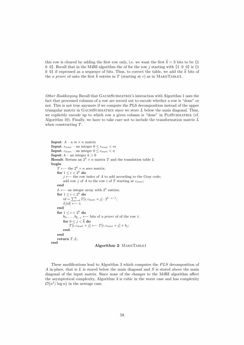
this row is cleared by adding the first row only, i.e. we want the first k = 3 bits to be [1

0 0]. Recall that in the M4RI algorithm the id for the row j starting with [1 0 0] is [10 0] if expressed as a sequence of bits. Thus, to correct the table, we add the k bits ofthe a priori id onto the first k entries in T (starting at c) as in MakeTable1.

Other Bookkeeping Recall that GaussSubmatrix’s interaction with Algorithm 1 uses thefact that processed columns of a row are zeroed out to encode whether a row is “done” ornot. This is not true anymore if we compute the PLS decomposition instead of the uppertriangular matrix in GaussSubmatrix since we store L below the main diagonal. Thus,we explicitly encode up to which row a given column is “done” in PlsSubmatrix (cf.Algorithm 10). Finally, we have to take care not to include the transformation matrix Lwhen constructing T .

Input: A – a m× n matrixInput: rstart – an integer 0 ≤ rstart < mInput: cstart – an integer 0 ≤ cstart < nInput: k – an integer k > 0Result: Retuns an 2k × n matrix T and the translation table Lbegin

T ←− the 2k × n zero matrix;for 1 ≤ i < 2k do

j ←− the row index of A to add according to the Gray code;add row j of A to the row i of T starting at cstart;

end

L←− an integer array with 2k entries;for 1 ≤ i < 2k do

id =∑k

j=0 T [i, cstart + j] · 2k−j−1;L[id]←− i;

end

for 1 ≤ i < 2k dob0, . . . , bk−1 ←− bits of a priori id of the row i;

for 0 ≤ j < k doT [i, cstart + j]←− T [i, cstart + j] + bj ;

end

endreturn T,L;

endAlgorithm 2: MakeTable1

These modifications lead to Algorithm 3 which computes the PLS decomposition ofA in-place, that is L is stored below the main diagonal and S is stored above the maindiagonal of the input matrix. Since none of the changes to the M4RI algorithm affectthe asymptotical complexity, Algorithm 3 is cubic in the worst case and has complexityO(n3/ log n

)in the average case.

58

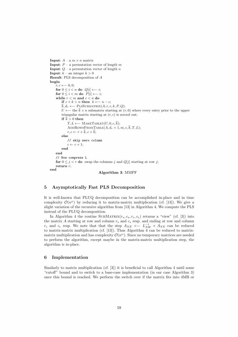
Input: A – a m× n matrixInput: P – a permutation vector of length mInput: Q – a permutation vector of length nInput: k – an integer k > 0Result: PLS decomposition of Abegin

r, c←− 0, 0;for 0 ≤ i < n do Q[i]←− i;for 0 ≤ i < m do P [i]←− i;while r < m and c < n do

if c+ k > n then k ←− n− c;k, dr ←− PlsSubmatrix(A, r, c, k, P,Q);U ←− the k × n submatrix starting at (r, 0) where every entry prior to the uppertriangular matrix starting at (r, c) is zeroed out;if k > 0 then

T,L←− MakeTable1(U, 0, c, k);AddRowsFromTable(A, dr + 1,m, c, k, T, L);r, c← r + k, c+ k;

else// skip zero column

c← c+ 1;end

end// Now compress L

for 0 ≤ j < r do swap the columns j and Q[j] starting at row j;return r;

endAlgorithm 3: MMPF

5 Asymptotically Fast PLS Decomposition

It is well-known that PLUQ decomposition can be accomplished in-place and in timecomplexity O(nω) by reducing it to matrix-matrix multiplication (cf. [13]). We give aslight variation of the recursive algorithm from [13] in Algorithm 4. We compute the PLSinstead of the PLUQ decomposition.

In Algorithm 4 the routine SubMatrix(rs, cs, re, ce) returns a “view” (cf. [3]) intothe matrix A starting at row and column rs and cs resp. and ending at row and columnre and ce resp. We note that that the step ANE ←− L−1NW × ANE can be reducedto matrix-matrix multiplication (cf. [13]). Thus Algorithm 4 can be reduced to matrix-matrix multiplication and has complexity O(nω). Since no temporary matrices are neededto perform the algorithm, except maybe in the matrix-matrix multiplication step, thealgorithm is in-place.

6 Implementation

Similarly to matrix multiplication (cf. [3]) it is beneficial to call Algorithm 4 until some“cutoff” bound and to switch to a base-case implementation (in our case Algorithm 3)once this bound is reached. We perform the switch over if the matrix fits into 4MB or

59

Input: A – a m× n matrixInput: P – a permutation vector of length mInput: Q – a permutation vector of length nResult: PLS decomposition of Abegin

n0 ←− pick some integer 0 ≤ n0 < n; // n0 ≈ n/2A0 ←− SubMatrix(A, 0, 0,m, n0);A1 ←− SubMatrix(A, 0, n0,m, n);Q0 ←− Q[0, . . . , n0];r0 ←− PLS(A0, P,Q0); // first recursive call

for 0 ≤ i ≤ n0 do Q[i]← Q0[i];ANW ←− SubMatrix(A, 0, 0, r0, r0);ASW ←− SubMatrix(A, r0, 0,m, r0);ANE ←− SubMatrix(A, 0, n0, r0, n);ASE ←− SubMatrix(A, r0, n0,m, n);if r1 then

// Compute of the Schur complement

A1 ←− P ×A1;LNW ←− the lower left triangular matrix in ANW ;ANE ←− L−1

NW ×ANE ;ASE ←− ASE +ASW ×ANE ;

endP1 ←− P [r0, . . . ,m];Q1 ←− Q[n0, . . . , n];r1 ←− PLS(ASE , P1, Q1); // second recursive call

ASW ←− P ×ASW ;// Update P & Q

for 0 ≤ i < m− r0 do P [r0 + 1] = P1[i] + r0;for 0 ≤ i < n− n0 do Q[n0 + i]← Q1[i] + n0;j ← r0;for n0 ≤ i < n0 + r1 do Q[j]← Q[i]; j ← j + 1;// Now compress L

j ← n0;for r0 ≤ i < r0 + r1 do swap the columns i and j starting at row i;return r0 + r1;

endAlgorithm 4: PLS Decomposition

60

in L2 cache, whichever is smaller. These values seem to provide the best performance onour target platforms.

The reason we are considering the PLS decomposition instead of either the LQUP orthe PLUQ decomposition is that the PLS decomposition has several advantages over F2,in particular when the flat row-major representation is used to store entries.

– We may choose where to cut with respect to columns in Algorithm 4. In particular, wemay choose to cut along word boundaries. For LQUP decomposition, where roughlyall steps are transposed, column cuts are determined by the rank r0.

– In Algorithm 3 rows are added instead of columns. Row operations are much cheaperthan column operations in row-major representation.

– Column swaps do not occur in the main loop of either Algorithm 4 or 3, but only rowswaps are performed. Column swaps are only performed at the end. Column swapsare much more expensive than row swaps (see below).

– Fewer column swaps are performed for PLS decomposition than for PLUQ decompo-sition since U is not compressed.

One of the major bottleneck are column swaps. In Algorithm 5 a simple algorithm forswapping two columns a and b is given with bit-level detail. In Algorithm 5 we assumethat the bit position of a is greater than the bit position of b for simplicity of presentation.The advantage of the strategy in Algorithm 5 is that it uses no conditional jumps in theinner loop, However, it still requires 9 instructions per row. On the other hand, we canadd two rows with 9 · 128 = 1152 entries in 9 instructions if the SSE2 instruction setis available. Thus, for matrices of size 1152 × 1152 it takes roughly the same number ofinstructions to add two matrices as it does to swap two columns. If we were to swapevery column with some other column once during some algorithm it thus would be asexpensive as a matrix multiplication for matrices of these dimensions.

Input: A – a m× n matrixInput: a – an integer 0 ≤ a < b < nInput: b – an integer 0 ≤ a < b < nResult: Swaps the columns a and b in Abegin

M ←− the memory where A is stored;aw, bw ←− the word index of a and b in M ;ab, bb ←− the bit index of a and b in aw and bw;∆←− ab − bb;am ←− the bit-mask where only the abth bit is set to 1;bm ←− the bit-mask where only the bbth bit is set to 1;for 0 ≤ i < m do

R←− the memory where the row i is stored;R[aw]←− R[aw]⊕ ((R[bw] bm) >> ∆);R[bw]←− R[bw]⊕ ((R[aw] am) << ∆);R[aw]←− R[aw]⊕ ((R[bw] bm) >> ∆);

endend

Algorithm 5: Column Swap

61

Another bottleneck for relatively sparse matrices in dense row-major representation isthe search for pivots. Searching for a non-zero element in a row can be relatively expensivedue to the need to identify the bit position. However, the main performance penalty isdue to the fact that searching for a non-zero entry in one column is in a row-majorrepresentation is very cache unfriendly.

Indeed, both our implementation and the implementation available in Magma sufferfrom performance regression on relatively sparse matrices as shown in Figure 2. We stressthat this is despite the fact that the theoretical complexity of matrix decomposition is ranksensitive, that is, strictly less field operations have to be performed for low rank matrices.While the penalty for relatively sparse matrices is much smaller for our implementationthan for Magma, it clearly does not achieve the theoretical possible performance. Thus,we also consider a hybrid algorithm which starts with M4RI and switches to PLS-basedelimination as soon as the (approximated) density reaches 15%, denoted as ‘M+P 0.15’.

0 10 20 30 40 50nonzero elements per row on average

0

2

4

6

8

10

12

14

execu

tion t

ime t

M4RIM+P 0.15PLSMagma

Fig. 2. Sensitivity to density for n = 104 on 2.6Ghz Opteron

7 Results

In Table 1 we give average running time over ten trials for computing reduced row echelonforms of dense random n × n matrices over F2. We compare the asymptotically fast im-plementation due to Allan Steel in Magma, the cubic Gaussian elimination implemented

62

by Victor Shoup in NTL, and both our implementations. Both the implementation inMagma and our PLS decomposition reduce matrix decomposition to matrix multiplica-tion. A discussion and comparison of matrix multiplication in the M4RI library and inMagma can be found in [3]. In Table 1 the column ‘PLS’ denotes the complete runningtime for first computing the PLS decomposition and the computation of the reduced rowechelon form from PLS.

64-bit Linux, 2.6Ghz Opteron 64-bit Linux, 2.33Ghz Xeon (E5345)

n Magma NTL M4RI PLS Magma NTL M4RI PLS2.15-10 5.4.2 20090105 20100324 2.16-7 5.4.2 20100324 20100324

10, 000 3.351s 18.45s 2.430s 1.452s 2.660s 12.05s 1.360s 0.864s16, 384 11.289s 72.89s 10.822s 6.920s 8.617s 54.79s 5.734s 3.388s20, 000 16.734s 130.46s 19.978s 10.809s 12.527s 100.01s 10.610s 5.661s32, 000 57.567s 479.07s 83.575s 49.487s 41.770s 382.52s 43.042s 20.967s64, 000 373.906s 2747.41s 537.900s 273.120s 250.193s – 382.263s 151.314s

Table 1. RREF for random matrices

In Table 2 we give running times for matrices as they appear when solving non-linearsystems of equations. The matrices HFE 25, 30 and 35 were contributed by MichaelBrickenstein and appear during a Grobner basis computation of HFE systems usingPolyBoRi. The Matrix MXL was contributed by Wael Said and appears during anexecution of the MXL2 algorithm [15] for a random quadratic system of equations. Weconsider these matrices within the scope of this work since during matrix elimination thedensity quickly increases and because even the input matrices are dense enough such thatwe expect one non-zero element per 128-bit wide SSE2 XOR on average. The columns‘M+P 0.xx’ denote the hybrid algorithms which start with M4RI and switch over to PLSbased echelon form computation once the density of the remaining part of the matrixreaches 15% or 20% respectively. We note that the relative performance of the M4RI andthe PLS algorithm for these instances depends on particular machine configuration. Todemonstrate this we give a set of timings for the Intel Xeon X7460 machine sage.math4

in Table 2. Here, PLS always is faster than M4RI, while on a Xeon E5345 M4RI wins forall HFE examples. We note that Magma is not available on the machine sage.math. TheHFE examples show that the observed performance regression for sparse matrices doeshave an impact in practice and that the hybrid approach does look promising for theseinstances.

8 Acknowledgments

We would like to thank anonymous referees for helpful comments on how to improve ourpresentation.

4 Purchased under National Science Foundation Grant No. DMS-0821725.

63

64-bit Fedora Linux, 2.33Ghz Xeon (E5345)

Problem Matrix Density Magma M4RI PLS M+P 0.15 M+P 0.20Dimension 2.16-7 20100324 20100324 20100429 20100429

HFE 25 12, 307× 13, 508 0.076 3.68s 1.94s 2.09s 2.33s 2.24sHFE 30 19, 907× 29, 323 0.067 23.39s 11.46s 13.34s 12.60s 13.00sHFE 35 29, 969× 55, 800 0.059 – 49.19s 68.85s 66.66s 54.42s

MXL 26, 075× 26, 407 0.185 55.15 12.25s 9.22s 9.22s 10.22s

64-bit Ubuntu Linux, 2.66Ghz Xeon (X7460)

Problem Matrix Density M4RI PLS M+P 0.15 M+P 0.20Dimension 20100324 20100324 20100429 20100429

HFE 25 12, 307× 13, 508 0.076 2.24s 2.00s 2.39s 2.35sHFE 30 19, 907× 29, 323 0.067 27.52s 13.29s 13.78s 22.9sHFE 35 29, 969× 55, 800 0.059 115.35s 72.70s 84.04s 122.65s

MXL 26, 075× 26, 407 0.185 26.61s 8.73s 8.75s 13.23s

64-bit Debian/GNU Linux, 2.6Ghz Opteron)

Problem Matrix Density Magma M4RI PLS M+P 0.15 M+P 0.20Dimension 2.15-10 20100324 20100324 20100429 20100429

HFE 25 12, 307× 13, 508 0.076 4.57s 3.28s 3.45s 3.03s 3.21sHFE 30 19, 907× 29, 323 0.067 33.21s 23.72s 25.42s 23.84s 25.09sHFE 35 29, 969× 55, 800 0.059 278.58s 126.08s 159.72s 154.62s 119.44s

MXL 26, 075× 26, 407 0.185 76.81s 23.03s 19.04s 17.91s 18.00sTable 2. RREF for matrices from practice.

References

1. A.V. Aho, J.E. Hopcroft, and J.D. Ullman. The Design and Analysis of Computer Algo-rithms. Addison-Wesley, 1974.

2. Martin Albrecht and Gregory V. Bard. The M4RI Library – Version 20091104. TheM4RI Team, 2009. http://m4ri.sagemath.org.

3. Martin Albrecht, Gregory V. Bard, and William Hart. Algorithm 898: Efficient multiplicationof dense matrices over GF(2). ACM Transactions on Mathematical Software, 37(1), 2009.pre-print available at http://arxiv.org/abs/0811.1714.

4. V. Arlazarov, E. Dinic, M. Kronrod, and I. Faradzev. On economical construction of thetransitive closure of a directed graph. Dokl. Akad. Nauk., 194(11), 1970. (in Russian), EnglishTranslation in Soviet Math Dokl.

5. Gregory V. Bard. Accelerating cryptanalysis with the Method of Four Russians. CryptologyePrint Archive, Report 2006/251, 2006. Available at http://eprint.iacr.org/2006/251.pdf.

6. Gregory V. Bard. Algorithms for Solving Linear and Polynomial Systems of Equations overFinite Fields with Applications to Cryptanalysis. PhD thesis, University of Maryland, 2007.

7. Gregory V. Bard. Matrix inversion (or LUP-factorization) via the Method of Four Russians,in θ(n3/ log(n)) time. In Submission, 2008.

8. Wieb Bosma, John Cannon, and Catherine Playoust. The MAGMA Algebra System I: TheUser Language. In Journal of Symbolic Computation 24, pages 235–265. Academic Press,1997.

9. Michael Brickenstein and Alexander Dreyer. PolyBoRi: A framework for Grobner basiscomputations with Boolean polynomials. In Electronic Proceedings of MEGA 2007, 2007.Available at http://www.ricam.oeaw.ac.at/mega2007/electronic/26.pdf.

10. Nicolas T. Courtois, Alexander Klimov, Jacques Patarin, and Adi Shamir. Efficient algo-rithms for solving overdefined systems of multivariate polynomial equations. In Advances

64

in Cryptology — EUROCRYPT 2000, volume 1807 of Lecture Notes in Computer Science,pages 392–407, Berlin, Heidelberg, New York, 2000. Springer Verlag.

11. Jean-Charles Faugere. A new efficient algorithm for computing Grobner basis (F4). Journalof Pure and Applied Algebra, 139(1-3):61–88, 1999.

12. O.H. Ibarra, S. Moran, and R. Hui. A generalization of the fast LUP matrix decompositionalgorithm and applications. Journal of Algorithms, 3:45–56, 1982.

13. Claude-Pierre Jeannerod, Clement Pernet, and Arne Storjohann. Fast gaussian eliminationand the PLUQ decomposition. in submission, 2010.

14. Mohamed Saied Emam Mohamed, Daniel Cabarcas, Jintai Ding, Johannes Buchmann, andStanislav Bulygin. Mxl3: An efficient algorithm for computing grobner bases of zero-dimensional ideals. In 12th International Conference on Information Security and Cryptology(ICISC), 2009.

15. Mohamed Saied Emam Mohamed, Wael Said Abd Elmageed Mohamed, Jintai Ding, andJohannes Buchmann. Mxl2: Solving polynomial equations over gf(2) using an improved mu-tant strategy. In Proceedings of Post-Quantum Cryptography 2008, 2008. pre-print availableat http://www.cdc.informatik.tu-darmstadt.de/reports/reports/MXL2.pdf.

16. William Stein et al. SAGE Mathematics Software (Version 4.3). The Sage DevelopmentTeam, 2008. Available at http://www.sagemath.org.

65

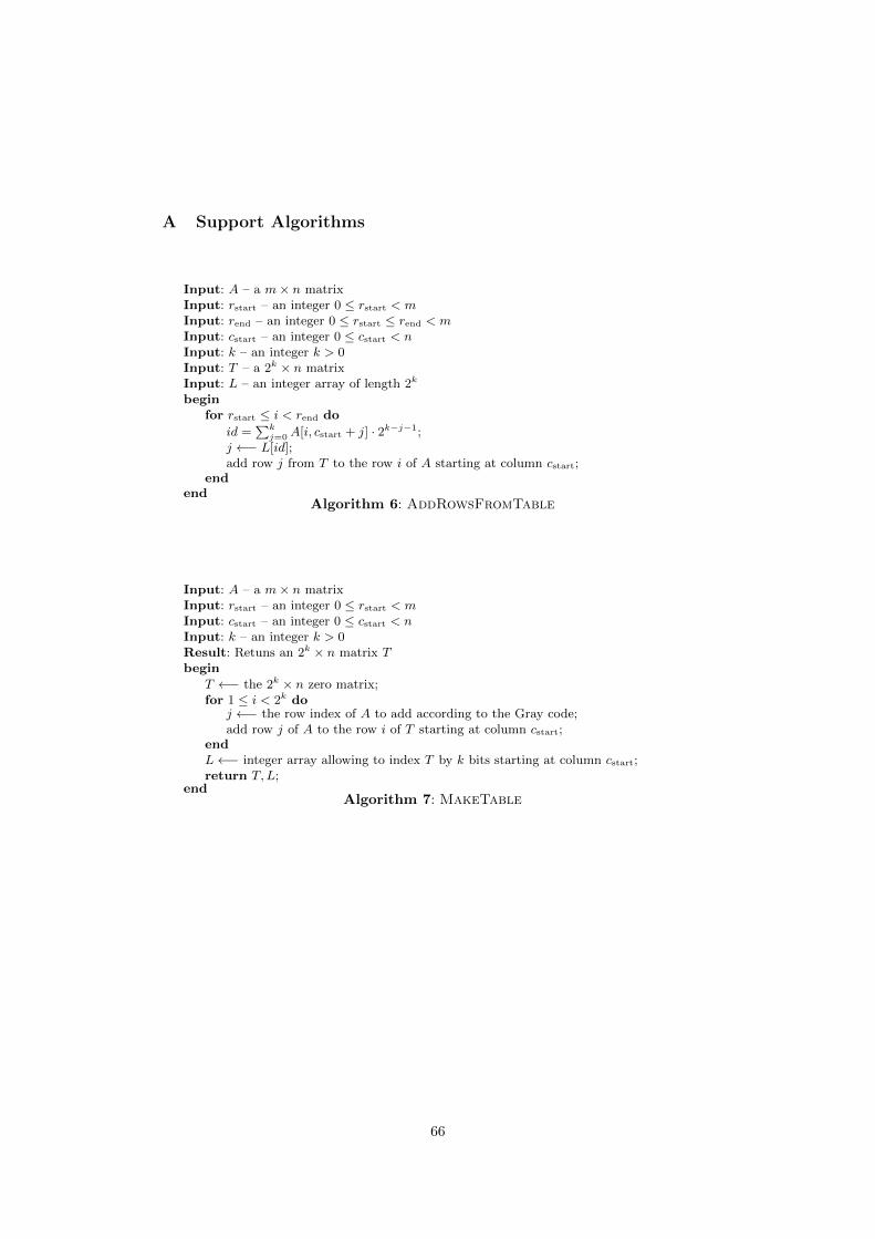
A Support Algorithms

Input: A – a m× n matrixInput: rstart – an integer 0 ≤ rstart < mInput: rend – an integer 0 ≤ rstart ≤ rend < mInput: cstart – an integer 0 ≤ cstart < nInput: k – an integer k > 0Input: T – a 2k × n matrixInput: L – an integer array of length 2k

beginfor rstart ≤ i < rend do

id =∑k

j=0A[i, cstart + j] · 2k−j−1;j ←− L[id];add row j from T to the row i of A starting at column cstart;

endend

Algorithm 6: AddRowsFromTable

Input: A – a m× n matrixInput: rstart – an integer 0 ≤ rstart < mInput: cstart – an integer 0 ≤ cstart < nInput: k – an integer k > 0Result: Retuns an 2k × n matrix Tbegin

T ←− the 2k × n zero matrix;for 1 ≤ i < 2k do

j ←− the row index of A to add according to the Gray code;add row j of A to the row i of T starting at column cstart;

endL←− integer array allowing to index T by k bits starting at column cstart;return T,L;

endAlgorithm 7: MakeTable

66

Input: A – a m× n matrixInput: r – an integer 0 ≤ r < mInput: c – an integer 0 ≤ c < nInput: k – an integer k > 0Input: rend – an integer 0 ≤ r ≤ rend < mResult: Returns the rank k ≤ k and puts the k × (n− c) submatrix starting at A[r, c] in

reduced row echelon form.begin

rs ←− r;for c ≤ j < c+ k do

found←− False;for rs ≤ i < rend do

for 0 ≤ l < j − c do // clear the first columnsif A[i, c+ l] 6= 0 then add row r+ l to row i of A starting at column c+ l;

endif A[i, j] 6= 0 then // pivot?

Swap the rows i and rs in A;for r ≤ l < rs do // clear above

if A[l, j] 6= 0 then add row rs to row l in A starting at column j;endrs ←− rs + 1;found←− True;break;

end

endif found = False then

return j - c;end

endreturn j - c;

endAlgorithm 8: GaussSubmatrix

67

Input: A – a m× n matrixInput: P – a permutation vector of length mInput: Q – a permutation vector of length nResult: PLS decomposition of A. Returns the rank of A.begin

r, c← 0, 0;while r < m and c < n do

found←− False;for c ≤ j < n do // search for some pivot

for r ≤ i < m doif A[i, j] then found← True and break;

endif found then break;

endif found then

P [r], Q[r]←− i, j;swap the rows r and i in A;// clear below but preserve transformation matrix

if j + 1 < n thenfor r + 1 ≤ l < m do

if A[l, j] thenadd the row r to the row l starting at column j + 1;

end

end

endr, c←− r + 1, j + 1;

elsebreak;

end

endfor r ≤ i < m do P [i]←− i ;for r ≤ i < n do Q[i]←− i ;// Now compress L

for 0 ≤ j < r do swap the columns j and Q[j] starting at row j;return r;

endAlgorithm 9: Gaussian PLS Decomposition

68

Input: A – a m× n matrixInput: sr – an integer 0 ≤ sr < mInput: sc – an integer 0 ≤ sc < nInput: k – an integer k > 0Input: P – a permutation vector of length mInput: Q – a permutation vector of length nResult: Returns the rank k ≤ k and dr – the last row considered.Also puts the k × (n− c) submatrix starting at (r, c) in PLS decomposition form.begin

done←− all zero integer array of length k;for 0 ≤ r < k do

found←− False;for sr + r ≤ i < m do // search for some pivot

for 0 ≤ l < r do // clear before

if done[l] < i thenif A[i, sc + l] 6= 0 then

add row sr + l to row i in A starting at column sc + l + 1;enddone[l]←− i;

end

endif A[i, sc + r] 6= 0 then

found←− True;break;

end

endif found = False then break;P [sr + r], Q[sr + r]←− i, sc + r;swap the rows sr + r and i in A;done[r]←− i;

end

dr ←− max(done[i] | i ∈ 0, . . . , k − 1);for 0 ≤ c2 < k and r + c2 < n− 1 do // finish submatrix

for done[c2] < r2 ≤ dr doif A[r2, r + c2] 6= 0 then

add row r + c2 to row r2 in A starting at column r + c2 + 1;end

end

endreturn r, dr;

endAlgorithm 10: PlsSubmatrix

69

Breaking Elliptic Curves Cryptosystems usingReconfigurable Hardware

Junfeng Fan†, Daniel V. Bailey‡∗ , Lejla Batina†/, Tim Guneysu‡, ChristofPaar‡ and Ingrid Verbauwhede†

† ESAT/SCD-COSIC, Katholieke Universiteit Leuven and IBBTKasteelpark Arenberg 10, B-3001 Leuven-Heverlee, Belgium

[email protected]‡ Horst Gortz Institute for IT Security, Ruhr University Bochum, Germany

gueneysu, [email protected]∗ RSA, the Security Division of EMC, USA

[email protected]/ Radboud University Nijmegen, Netherlands

Abstract. This paper reports a new speed record for FPGAs in crackingElliptic Curve Cryptosystems. We conduct a detailed analysis of differentF2m multiplication approaches in this application. A novel architectureusing optimized normal basis multipliers is proposed to solve the Certi-com challenge ECC2K-130. We compare the FPGA performance againstCPUs, GPUs, and even the Sony PlayStation 3. Our implementationsshow low-cost FPGAs outperform even multicore desktop processors andgraphics cards by a factor of 2.

1 Motivation: Attacking ECC2K-130

Cryptosystems ensure the security, authenticity and privacy of data and users inmost products nowadays. Elliptic-Curve Cryptosystems (ECC), independentlyinvented by Miller [18] and Koblitz [15], are now commonplace in both theacademic literature and practical deployments. These systems allow shorter key-lengths, ciphertexts, and signatures than other conventional cryptosystems, e.g.,RSA. In addition, thanks to these smaller operands, ECC offer higher perfor-mance and lower power when compared with other systems. Especially in per-vasive computing applications, ECC admit valuable optimizations in computingand communication complexity.

The security of ECC relies on the difficulty of Elliptic Curve Discrete Log-arithm Problem (ECDLP) [3]. Briefly speaking, ECDLP is to find an integer nfor two points P and Q on an elliptic curve E such that Q ≡ [n]P . To use ECCin the real world, practitioners need to know: how big should the parameters (or,colloquially, the ”key size”) be to avoid practical attacks? Choosing parameterstoo small allows computational attackers to solve the ECDLP instance, whilechoosing parameters too large wastes time, communication, and storage. To en-courage investigation of these issues, researchers at Certicom Corp. published alist of ECDLP challenges in 1997 [7].

71

Smaller members of the list of Certicom ECDLP challenge problems havebeen solved. Escott et al. report on their successful attack on ECCp-97, anECDLP in a group of roughly 297 elements [8]. A larger instance, ECC2-109 wassolved by Monico et al. [6]. Bos et al. analyze and solve the ECDLP in a groupof roughly 2112 elements using PS3 [4].

This paper reports on our effort to solve one of the Certicom ECDLP chal-lenge problems using FPGAs. We focus on the ECC2K-130 challenge. ECC2K-130 is a Koblitz curve challenge over F2131 . Compared to previous attacks, whichare mostly implemented in software on general-purpose workstations, our workobtains a much higher performance-cost ratio by using FPGA platforms.

The rest of the paper is organized as follows. Section 2 summarizes relatedwork. In Section 3 we give a short description of the function that we imple-ment on FPGA. Section 4 and 5 explore different algorithms and architectures.Section 6 reports on the results, and finally we conclude the paper in Section 7.

2 Related Work

The strongest known attacks against the ECDLP are generic attacks based onPollard’ rho method [20, 5]. Further improvements including parallelization andthe use of group automorphisms were made by Wiener and Zuccherato [26], vanOorschot et al. [25], and Gallant et al. [9]. The parallelized Pollard rho methodconsists of parallel loops that search for distinguished points. Each loop startsfrom a random point on E and ends when a distinguished point is hit. The corefunction is thus the update function, also known as iteration function. Our workimplements this function along with its improvements.

FPGAs have been applied to the Pollard rho method in several previousworks. Guneysu et al. analyze ECDLPs over fields of odd-prime characteris-tic [11, 10], targeting a machine with 128 low-cost FPGAs. They extrapolatethat to break an ECDLP in a group of roughly 2131 elements using this machineas taking over a thousand years.

Similarly, Meurice de Dormale et al. apply FPGAs to the ECDLP [17]. Here,they use characteristic-two finite fields, but restrict their inquiry to polynomialbasis. Although conventional wisdom has held that low-weight polynomial basisis a better choice, in our application we can take advantage of the free repeatedsquarings (2n-th powers) offered in normal basis. In addition, recent progress onnormal-basis multiplication by Shokrollahi et al. [24] and Bernstein and Lange[2] further improve the prospects for normal basis. Our work is the first FPGAimplementation of parallelized Pollard rho method using normal basis multipli-cation.

This work is part of a global distributed effort to break the largest ECDLPever solved [1]. While that paper summarizes the overall effort, here we focus onthe FPGA implementation.

The Contribution of This Paper. As part of this effort, this paper ex-plores FPGA implementation options for the core finite-field arithmetic opera-tions as well as architectures. An in-depth comparison between polynomial basis

72

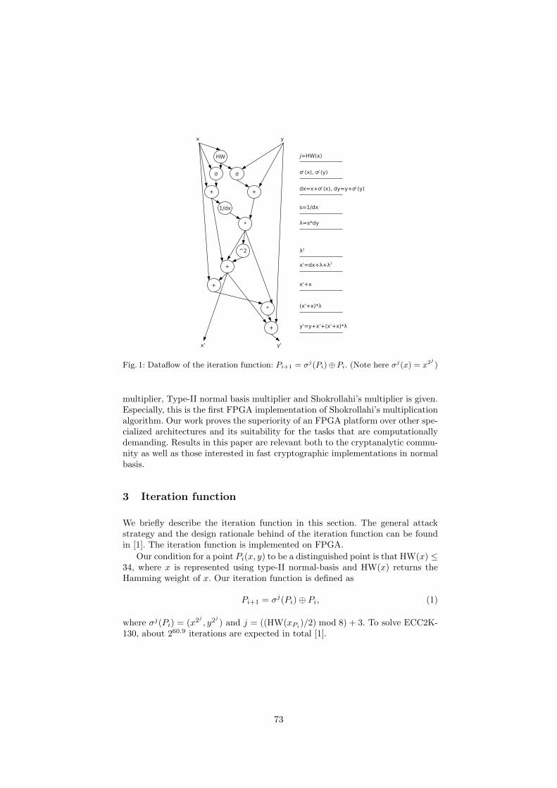
Fig. 1: Dataflow of the iteration function: Pi+1 = σj(Pi)⊕Pi. (Note here σj(x) = x2j

)

multiplier, Type-II normal basis multiplier and Shokrollahi’s multiplier is given.Especially, this is the first FPGA implementation of Shokrollahi’s multiplicationalgorithm. Our work proves the superiority of an FPGA platform over other spe-cialized architectures and its suitability for the tasks that are computationallydemanding. Results in this paper are relevant both to the cryptanalytic commu-nity as well as those interested in fast cryptographic implementations in normalbasis.

3 Iteration function

We briefly describe the iteration function in this section. The general attackstrategy and the design rationale behind of the iteration function can be foundin [1]. The iteration function is implemented on FPGA.

Our condition for a point Pi(x, y) to be a distinguished point is that HW(x) ≤34, where x is represented using type-II normal-basis and HW(x) returns theHamming weight of x. Our iteration function is defined as

Pi+1 = σj(Pi)⊕ Pi, (1)

where σj(Pi) = (x2j

, y2j

) and j = ((HW(xPi)/2) mod 8) + 3. To solve ECC2K-

130, about 260.9 iterations are expected in total [1].

73

An efficient implementation of the iteration function is thus the key steptowards a fast attack. Given Pi(x, y), the iteration function computes Pi+1(x′, y′)using Eq.(1). Fig. 1 shows the data flow of the iteration function.

4 Optimizing Finite-Field Operations

The iteration function consists of two multiplications, one inversion and severalsquarings in F2m . Thus, fast finite-field arithmetic is essential to optimize theattack.

A vast body of literature exists on finite field arithmetic, and we are free tochoose from a variety of representations and algorithms. For example, we canuse either polynomial basis or normal basis for element representation, and aniteration can be performed using eithr Extended Euclidean Algorithm (EEA) orFermat’s little theorem. This leads to an important question: which configuration(basis, multiplication algoirthm, inversion algorithm) ensures the most efficientimplementation of the aforementioned iteration function? We try to answer thisquestion with complexity analysis and design-space exploration.

4.1 Multiplication

An element of F2131 can be represented in both polynomial basis P and Type-IInormal basis N, where

P = 1, w, w2, · · · , w130,N = γ + γ−1, γ2 + γ−2, γ2

2

+ γ−22

, · · · , γ2130 + γ−2130.

Here w is a root of an irreducible polynomial of degree 131, while γ is a primitive263rd root of unity. Multiplication in polynomial basis has long been consideredmore efficient than normal basis. On the other hand, squaring in normal basis issimply a circular shift. Moreover, computing any power α2n can be performed bycircularly-shifting by n positions. We implemented both options for comparison.

Besides conventional multiplication algorithms in polynomial and normal ba-sis, we also implemented a recently reported hybrid algorithm, due to Shokrol-lahi [24]. This algorithm uses only O(m logm) operations for the basis conversion.When multiplication is needed, two field elements are converted to polynomialbasis, a polynomial-basis multiplication is carried out, then the results are con-verted back to normal basis and reduced. This paper includes the first FPGAimplementation of this method.

Polynomial-Basis Multiplier Algorithms for multiplication in polynomialbasis consist of two steps, polynomial multiplication and modular reduction.They can be carried out separately or interleaved. Given two elements A(w) =m−1∑

i=0

aiwi and B(w) =

m−1∑

i=0

biwi, a bit-serial modular multiplication algorithm is

shown in Alg. 1.

74

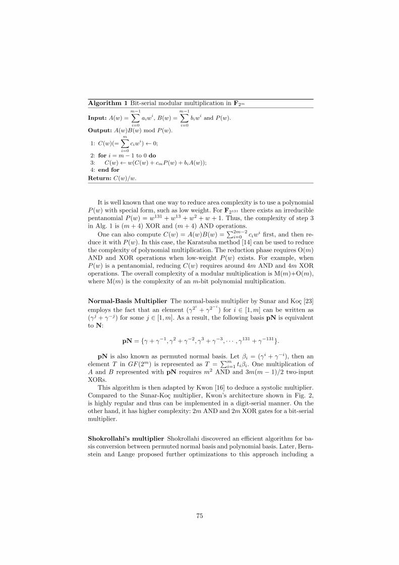
Algorithm 1 Bit-serial modular multiplication in F2m

Input: A(w) =

m−1Xi=0

aiwi, B(w) =

m−1Xi=0

biwi and P (w).

Output: A(w)B(w) mod P (w).

1: C(w)(=mXi=0

ciwi)← 0;

2: for i = m− 1 to 0 do3: C(w)← w(C(w) + cmP (w) + biA(w));4: end for

Return: C(w)/w.

It is well known that one way to reduce area complexity is to use a polynomialP (w) with special form, such as low weight. For F2131 there exists an irreduciblepentanomial P (w) = w131 + w13 + w2 + w + 1. Thus, the complexity of step 3in Alg. 1 is (m+ 4) XOR and (m+ 4) AND operations.

One can also compute C(w) = A(w)B(w) =∑2m−2

i=0 ciwi first, and then re-

duce it with P (w). In this case, the Karatsuba method [14] can be used to reducethe complexity of polynomial multiplication. The reduction phase requires O(m)AND and XOR operations when low-weight P (w) exists. For example, whenP (w) is a pentanomial, reducing C(w) requires around 4m AND and 4m XORoperations. The overall complexity of a modular multiplication is M(m)+O(m),where M(m) is the complexity of an m-bit polynomial multiplication.

Normal-Basis Multiplier The normal-basis multiplier by Sunar and Koc [23]

employs the fact that an element (γ2i

+ γ2−i

) for i ∈ [1,m] can be written as(γj + γ−j) for some j ∈ [1,m]. As a result, the following basis pN is equivalentto N:

pN = γ + γ−1, γ2 + γ−2, γ3 + γ−3, · · · , γ131 + γ−131.

pN is also known as permuted normal basis. Let βi = (γi + γ−i), then anelement T in GF (2m) is represented as T =

∑mi=1 tiβi. One multiplication of

A and B represented with pN requires m2 AND and 3m(m − 1)/2 two-inputXORs.

This algorithm is then adapted by Kwon [16] to deduce a systolic multiplier.Compared to the Sunar-Koc multiplier, Kwon’s architecture shown in Fig. 2,is highly regular and thus can be implemented in a digit-serial manner. On theother hand, it has higher complexity: 2m AND and 2m XOR gates for a bit-serialmultiplier.

Shokrollahi’s multiplier Shokrollahi discovered an efficient algorithm for ba-sis conversion between permuted normal basis and polynomial basis. Later, Bern-stein and Lange proposed further optimizations to this approach including a

75

Fig. 2: Modular multiplier in GF (2m) using Kwon’s algorithm

more straight-forward conversion function. More details on this multiplicationmethod can be found in their recent work [2]. The new polynomial basis (nP)is defined in [2] as Type-II polynomial basis.

nP = (γ + γ−1), (γ + γ−1)2, · · · , (γ + γ−1)m

which leads to a hybrid normal-basis multiplication algorithm. We denote AnP

and ApN the representation of A using nP and pN, respectively. A multiplicationthen proceeds as follows.

1. converting to polynomial basis: AnP ← ApN , BnP ← BpN ,2. polynomial multiplication: CnP ← AnPBnP ,3. converting back to normal basis (2m-bit conversion): CpN ← CnP ,4. reduction (folding).

Let SpN2nP be a transformation function that converts ApN to AnP . Theessential observation by Shokrollahi is that basis conversion can be recursivelybroken down to half-length transformations. Let fpN and fnP be correspondingrepresentations of f in pN and nP, respectively,

fpN = [f1 f2 · · · f8] [(γ + γ−1) (γ2 + γ−2) · · · (γ8 + γ−8)]T ,

fnP = [g1 g2 · · · g8] [(γ + γ−1) (γ + γ−1)2 · · · (γ + γ−1)8]T ,

Converting fpN to fnP can be then performed with two 4-bit transformations:

g1, g2, g3, g4nPSpN2nP←−−−−− f1 + f7, f2 + f6, f3 + f5, f4pN

g5, g2, g7, g8nPSpN2nP←−−−−− f5, f6, f7, f8pN

The pN → nP and nP → pN conversion in F2m takes (m/2) log2(m/4)operations each. In total, one field multiplication takes about M(m)+m log2m+m log2(m/4) operations. A more detailed discussion on the complexity can befound in [2].

Based on the analysis above, we can draw the following conclusions:

– A bit-serial multiplier using polynomial basis has a lower area complexitythan one using normal basis.

76

Fig. 3: Shokrollahi multiplier

– When low-weight polynomials exist, Shokrollahi’s multiplication algorithmis likely to have a higher complexity than convential polynomial basis multi-plication since the base conversion step is more complex than the polynomialreduction.

Though it seems that polynomial basis should be used, normal basis offersseveral advantages in this specific application. First, the Pollard rho iterationfunction requires the Hamming weight of x-coordinate represented in normalbasis. In fact, thanks to the Frobenius endomorphism, checking HW of x innormal basis checks 131 points simultaneously. This brings a speedup of

√131 to

the attack [1]. Second, the iteration function includes two σ(x, j) = x2j

routines(known as m-squaring). In normal basis, σ is essentially a circular shift of j bits,and thus can be performed in one cycle. Gains in m-squaring compensate theloss in multiplications.

4.2 Inversion

Inversion is the most costly of the four basic field operations. Two broad ap-proaches are found in the literature: the Extended Euclidean Algorithm (EEA)and Fermat’s Little Theorem (FLT). In polynomial basis, the binary variant ofEEA is generally faster, while the variant of FLT attributed to Itoh and Tsu-jii [13] is the better choice in normal basis because squaring is free. Itoh-Tsujiireduces the problem of extension-field inversion to exponentiation and inversionin the subfield. In polynomial basis, exponentiation is generally quite expensiveowing to the need to explicitly compute squares, making EEA a better choice.Itoh-Tsujii raises an element to the exponent r− 1 = 2 + 22 + · · ·+ 2m−1, usingthe fact that in normal basis, squaring is free. In addition, this algorithm usesan addition chain to reduce the number of multiplications: in F2131 , our addi-

77

Algorithm 2 Simultaneous inversion (Batch size = 3)

Input: α1, α2, α3.Output: α−1

1 , α−12 and α−1

3 .

1: d1 ← α1

2: d2 ← d1α2

3: d3 ← d2α3

4: u← d−13

5: t3 ← ud2, u← uα3

6: t2 ← ud1, u← uα2

7: t1 ← u

Return: t1, t2, t3.

tion chain has length nine (1, 2, 4, 8, 16, 32, 64, 128, 130). The net result is acomplexity of eight field multiplications to compute an inverse.

To further reduce the computation costs for inverses, we employ Mont-gomery’s trick that batches multiple inversions by trading inversions for mul-tiplications [19]. Alg.2 shows this method to invert three inputs. Indeed, we cantrade one inversion for three extra multiplications. As a result, one iterationfunction uses 5M + (1/n)I where n is the batch size.

5 Architecture Exploration

The architecture of the engine has a fundamental impact on the overall through-put. Among all the design options the following three are of great importance.

1. Multiplier architecture2. Memory architecture3. Inverter architecture

As an architecture exploration, we implemented three different architecturesusing different types of multipliers.

5.1 Architecture I: Load-Store

As a starting point, we take a programmable elliptic-curve coprocessor as theplatform. A digit-serial polynomial multiplier (see [21] for details) is used. Adedicated squarer is included for squaring. In each loop, the x-coordinate is con-verted into its normal basis representation, and its Hamming weight is counted.This adds a base conversion block and a Hamming weight computation block.

On this platform, squaring or addition takes two clock cycles, while multi-plication takes bn/dc + 1 cycles given a digit-size d. The design is synthesizedusing ISE 11.2 and the target FPGA is Xilinx Spartan-3 XC3S5000 (4FG676).Implementation results show that d = 22 gives the best trade-off in terms ofarea-delay product.

78

Fig. 4: Archi-I : ECC processor using polynomial basis multiplier

The design consumes 3,656 slices, including 1,468 slices for the multiplier, 75slices for the squarer, 1,206 slices for the base conversion, 117 slices for Hammingweight calculation.

One Pollard rho iteration takes 71 cycles, among them 35 cycles are usedfor multiplication. The design achieves a maximum clock frequency of 101 MHz,and one iteration takes 704 ns. The m-squaring is performed with m successivesquarings. Obviously, this architecture is not efficient. Them-squaring operationscan be largely sped up when normal basis is used.

5.2 Architecture II: Type-II Normal Basis Multiplier

Archi-II uses a digit-serial normal basis multiplier. The structure of the multi-plier is shown in Fig. 2. When m is small, a full systolic architecture can be used,performing one multiplication per cycle. However, a systolic array for F2131 istoo large (more than 20,000 slices on Spartan-3). Thus, a digit-serial architec-ture is used. Implementation results show that d = 13 gives the lowest area-delayproduct. The multiplier alone uses 2,093 slices.

The basis-conversion component in Archi-I is no longer needed in Archi-II,saving 1,468 slices. In total, the design uses 2,578 slices. On this platform, onePollard rho iteration takes 81 cycles, including 55 cycles used for multiplication.Compared to Archi-I, the m-squaring operation is largely improved. However,the multiplier becomes much slower than that in Archi-I. The design achieves amaximum clock frequency of 125 MHz, and one iteration takes 648 ns.

5.3 Architecture III: Fully Pipelined Iteration Function

Archi-III unrolls the Pollard rho iteration such that a throughput of one iter-ation per cycle is achieved. Remember that 5 multiplications are required foreach iteration, as a result, five normal basis multipliers are used. The design isfully pipelined. Since additions and squarings are embedded in the pipeline, itincreases the delay of one iteration but does not affect the throughput.

79

Fig. 5: Archi-II : ECC processor using normal basis

Fig. 6: Archi-III : pipelined processor using Shokrollahi multipliers

At the first glance, fully expanding the iteration function seams impossibledue to the inversion in each iteration. Indeed, after dx is generated in Fig.1,inverting dx will take too much area to fit one FPGA. The solution is to startthe pipeline after the real inversion (u← d−1n ) is performed.

Fig 6 shows the architecture that supports the expanded iteration function.In total, five multipliers are used. Before the starting of the pipeline, x,y,dx anddy of Pi are stored in RAM (x), (y), (dx) and (dy), respectively. RAM (dn)

80

keeps the intermediate data di of Alg. 2, and u is ready in register Ru. After thestarting of the pipeline, the five multipliers perform the following operations.

– Mul 1: ti ← udi−1– Mul 2: u← uαi

– Mul 3: λ← dy(1/dx)– Mul 4: λ(x′ + x)– Mul 5: d′i ← d′idx

′

Mul 1, Mul 2 and Mul 5 are used by batch inversion (Alg. 2), while Mul 3 andMul 4 are used for point addition (Fig. 1).

The inversion (u ← d−1n ) is performed by another multiplier together witha squarer. In order to keep full use of the engine, we interleave two groupsof iteration function. When the engine is executing one group, the inverter isperforming inversion for the other group.

The implementation of Archi-III consumes 22,195 slices and 20 block RAMs(RAMB16s) on Xilinx Spartan-3 XC3S5000 FPGA. One fully pipelined Shokrol-lahi’s multiplier uses 4,391 slices. The inverter itself uses 4,761 slices. In total,the design uses 26,731 slices. The post placing-and-routing results show that thisdesign can achieve a maximum clock frequency of 111 MHz.

6 Results and Analysis

The ECC2K-130 attack using FPGAs is conducted using an improved version ofthe COPACOBANA cluster described in [10, 12], also known as RIVYERA [22].It is populated with 128 Spartan-3 XC3S5000 FPGAs and an optional 32MBmemory per FPGA combined in one 19” housing. All FPGAs are connected withtwo opposite directed, systolic ring networks that directly interface with the PC(which is integrated in the same housing) via two individual PCI Express com-munication controllers. Although this setup can obviously provide a significantamount of bandwidth due to its local communication paths, the ECC2K-130attack design actually requires only moderate communication performance.

Table 1 summarizes the implementation results on a Spartan-3 XC3S5000FPGA. Based on the available resources (33,280 slices and 104 BRAMs) of eachXC3S5000 FPGA, we also estimated that at most 9 clones of Archi-I or 12 clonesof Archi-II can be implemented on a single FPGA. For Archi-III, one clone uses80% of the available resources of one FPGA.

Table 1: Cost for one Pollard’s rho iteration for various architectures

Digit Area Freq. Delay per Step Throughputsize #slice #BRAM [MHz] Cycles [ns] per FPGA

Archi-I : Polynomial basis 22 3,656 4 101 71 703 12.8 ×106

Archi-II : Type-II ONB 13 2,578 4 125 81 648 18.5 ×106

Archi-III : Shokrollahi’s - 26,731 20 111 23 (stages) 206 111 ×106

81

The throughput per engine, Te is computed as Te = Freq.Cycles per step , and the

throughput per FPGA Tc is computed as Tc = Te ∗ l. Here, l is the number ofengines on a single FPGA. Compared with Archi-I, Archi-II has smaller areaand shorter delay. In other words, Type-II optimal normal basis has significantadvantages for this application. On the other hand, Archi-III achieves a 8.6times speedup over Archi-II. The improvement mainly comes from the efficientfield arithmetic and the special architecture. The use of Shokrollahi’s algorithmsignificantly improved the throughput of a multiplier, while the expansion of theiteration function hides delays caused by addition and squaring in the pipeline.

Table 2: Performance comparison

Source Platform Challenge Frq. Throughput[MHz] [×106]

[17] Xilinx FPGA ECC2-131 100 10.0S3E1200-4

[1] Cell CPU ECC2K-130 3,200 27.76 SPEs, 1 PPE

[1] Graphics Card ECC2K-130 1,242 54.0GTX 295

[1] Core 2 Extreme ECC2K-130 3,000 22.5Q6850, 4 cores

This work Xilinx FPGA ECC2K-130 111 111(Archi-III ) XC3S5000

In Table 2 we compare our results with similar implementations on differentplatforms.

To our knowledge, this is the first FPGA implementation using fast normal-basis multiplication to attack ECDLP. As a point of comparison, we look intothe work of Meurice de Dormale, et al. [17]. They do not specifically targetKoblitz curves and they are using different FPGAs, which makes a fair compar-ison difficult.

On the other hand, there is an interesting comparison between implemen-tations of the same attack (and thus iteration function) on different platformsother than FPGAs. Within the whole project [1] efforts have been made tospeed-up the iteration function on CPUs, GPUs and PlayStation 3. These plat-forms are state-of-the-art processors supporting massive parallelism. Comparedto these platforms, our FPGA implementation is at least 2 times faster in termsof throughput.

The whole complexity of this attack is around 260.9 iterations. We estimatethat given five RIVYERA FPGA clusters, the ECC2K-130 challenge can besolved in one year.

82

7 Conclusion

A new efficiency record for FPGAs in cracking public-key cryptosystems basedon elliptic curves is reported. We conduct a detailed comparison of different ar-chitectures for normal-basis multipliers suited this application. The comparisonincludes the first FPGA implementation report for one of these architectures.Our results show that even low-cost FPGAs outperform CPUs, the PlayStation3 platform and even GPUs.

Acknowledgements

This work was supported in part by K.U. Leuven-BOF (OT/06/40), by the IAPProgramme P6/26 BCRYPT of the Belgian State (Belgian Science Policy), byFWO project G.0300.07, and by the European Commission through the ICTprogramme under contract ICT-2007-216676 ECRYPT II.

References

1. D. V. Bailey, L. Batina, D. J. Bernstein, P. Birkner, J. W. Bos, H. Chen, C. Cheng,G. van Damme, G. de Meulenaer, L. J. D. Perez, J. Fan, T. Guneysu, F. Gurkay-nak, T. Kleinjung, T. Lange, N. Mentens, R. Niederhagen, C. Paar, F. Regazzoni,P. Schwabe, L. Uhsadel, A. Van Herrewege, and B. Yang. Breaking ECC2K-130.Cryptology ePrint Archive, Report 2009/541, 2009. http://eprint.iacr.org/.

2. D.J. Bernstein and T. Lange. Type-II Optimal Polynomial Bases. to appear inWAIFI 2010 - http://binary.cr.yp.to/opb-20100209.pdf.

3. I. Blake, G. Seroussi, and N. Smart. Advances in Elliptic Curve Cryptography(London Mathematical Society Lecture Note Series). Cambridge University Press,New York, NY, USA, 2005.

4. J. W. Bos, M. E. Kaihara, T. Kleinjung, A. K. Lenstra, and P. L. Montgomery.On the security of 1024-bit RSA and 160-bit elliptic curve cryptography: version2.1. Cryptology ePrint Archive, Report 2009/389, 2009. http://eprint.iacr.

org/2009/389.5. R. P. Brent and J. M. Pollard. Factorization of the eighth Fermat number. Math-

ematics of Computation, 36:627–630, 1981.6. Certicom. Certicom ECC Challenge. http://www.certicom.com/images/pdfs/

cert_ecc_challenge.pdf, 1997.7. Certicom. ECC Curves List. http://www.certicom.com/index.php/curves-list,

1997.8. A. Escott, J. Sager, A. Selkirk, and D. Tsapakidis. Attacking elliptic curve cryp-

tosystems using the parallel Pollard rho method. CryptoBytes (The technicalnewsletter of RSA Laboratories), 4:15–19, 1998.

9. R. P. Gallant, R. J. Lambert, and S. A. Vanstone. Improving the parallelizedPollard lambda search on anomalous binary curves. Mathematics of Computation,69(232):1699–1705, 2000.

10. T. Guneysu, T. Kasper, M. Novotny, C. Paar, and A. Rupp. Cryptanalysis withCOPACOBANA. IEEE Transactions on Computers, 57(11):1498–1513, November2008.

83

11. T. Guneysu, C. Paar, and J. Pelzl. Attacking elliptic curve cryptosystems withspecial-purpose hardware. In Proceedings of the 2007 ACM/SIGDA 15th interna-tional symposium on Field programmable gate arrays, page 215. ACM, 2007.

12. T. Guneysu, G. Pfeiffer, C. Paar, and M. Schimmler. Three Years of Evolution:Cryptanalysis with COPACOBANA. In Workshop on Special-purpose Hardwarefor Attacking Cryptographic Systems - SHARCS 2009, September 9-10 2009.

13. T. Itoh and S. Tsujii. A Fast Algorithm for Computing Multiplicative Inverses inGF (2m) Using Normal Bases. Inf. Comput., 78(3):171–177, 1988.

14. A. Karatsuba and Y. Ofman. Multiplication of many-digital numbers by automaticcomputers. 145:595–596, 7 1963.

15. N. Koblitz. Elliptic curve cryptosystems. Mathematics of computation,48(177):203–209, 1987.

16. S. Kwon. A low complexity and a low latency bit parallel systolic multiplier overGF(2m) using an optimal normal basis of type II. In IEEE Symposium on Com-puter Arithmetic - ARITH-16, pages 196–202, 2003.

17. G. Meurice de Dormale, P. Bulens, and J. J. Quisquater. Collision Search for Ellip-tic Curve Discrete Logarithm over GF(2m) with FPGA. In Workshop on Crypto-graphic Hardware and Embedded Systems (CHES 2007), pages 378–393. Springer,2007.

18. V.S. Miller. Use of elliptic curves in cryptography. In Advances in CryptologyCRYPTO 85 Proceedings, pages 417–426, 1986.

19. P. L. Montgomery. Speeding the Pollard and elliptic curve methods of factorization.Mathematics of Computation, 48:243–264, 1987.

20. J. M. Pollard. Monte Carlo methods for index computation (mod p). Mathematicsof Computation, 32:918–924, 1978.

21. K. Sakiyama, L. Batina, B. Preneel, and I. Verbauwhede. Multicore Curve-Based Cryptoprocessor with Reconfigurable Modular Arithmetic Logic Units overGF(2n). IEEE Trans. Computers, 56(9):1269–1282, 2007.

22. SciEngines GmbH. RIVYERA S3-5000, 2010. http://www.sciengines.com/

joomla/index.php?option=com_content&view=article&id=60&Itemid=74.23. B. Sunar and C.K. Koc. An Efficient Optimal Normal Basis Type II Multiplier.

IEEE Transactions on Computers, 50:83–87, 2001.24. J. v. z. Gathen, A. Shokrollahi, and J. Shokrollahi. Efficient multiplication using

type 2 optimal normal bases. In Claude Carlet and Berk Sunar, editors, WAIFI,volume 4547 of Lecture Notes in Computer Science, pages 55–68. Springer, 2007.

25. P. C. van Oorschot and M. J. Wiener. Parallel collision search with cryptanalyticapplications. Journal of Cryptology, 12(1):1–28, 1999.

26. M. J. Wiener and R. J. Zuccherato. Faster attacks on elliptic curve cryptosystems.In Selected Areas in Cryptography, volume 1556 of LNCS, pages 190–200, 1998.

84

Fast Exhaustive Search for Polynomial Systems in F2

Charles Bouillaguet1, Hsieh-Chung Chen2, Chen-Mou Cheng3,Tung Chou3, Ruben Niederhagen3,4, Adi Shamir1,5, and Bo-Yin Yang2

1 Ecole Normale Supérieure, Paris, France, [email protected] Institute of Information Science, Academia Sinica, Taipei, Taiwan, kc,[email protected]

3 National Taiwan University, Taipei, Taiwan, doug,[email protected] Technische Universiteit Eindhoven, the Netherlands, [email protected]

5 Weizmann Institute of Science, Israel, [email protected]

Abstract. We analyze how fast we can solve general systems of multivariate equations of variouslow degrees over F2; this is a well known hard problem which is important both in itself and as partof many types of algebraic cryptanalysis. Compared to the standard exhaustive search technique, ourimproved approach is more efficient both asymptotically and practically. We implemented severaloptimized versions of our techniques on CPUs and GPUs. Our technique runs more than 10 timesfaster on modern graphic cards than on the most powerful CPU available. Today, we can solve 48+quadratic equations in 48 binary variables on a 500-dollar NVIDIA GTX 295 graphics card in 21minutes. With this level of performance, solving systems of equations supposed to ensure a securitylevel of 64 bits turns out to be feasible in practice with a modest budget. This is a clear demonstra-tion of the computational power of GPUs in solving many types of combinatorial and cryptanalyticproblems.Keywords: multivariate polynomials, solving systems of equations, exhaustive search, paralleliza-tion, Graphic Processing Units (GPUs)

1 Introduction

Solving a system of m nonlinear polynomial equations in n variables over Fq is a natural mathematicalproblem that has been investigated by various research communities. The cryptographers are among theinterested parties since an NP-complete problem whose random instances seem hard could be used todesign cryptographic primitives, as witness the development of multivariate cryptography in the last fewdecades, using one-way trapdoor functions such as HFE, SFLASH, and QUARTZ [13, 22, 23], as well asstream ciphers such as QUAD [5].

Conversely, in “algebraic cryptanalysis” one distills from a cryptographic primitive a system of mul-tivariate polynomial equations with the secret among the variables. This does not break AES as firstadvertised, but does break KeeLoq [12], for a recent example, and find a faster collision on 58-roundSHA-1 [26].

Since the pioneering work by Buchberger [10], Gröbner-basis techniques have been the most promi-nent tool for this problem, especially after the emergence of faster algorithms such as F4 or F5 [16, 17],which broke the first HFE challenge [18]. The cryptographic community independently rediscoveredsome of the ideas underlying efficient Gröbner-basis algorithms as of the XL algorithm [14] and its vari-ants. They also introduced techniques to deal with special cases, particularly that of sparse systems [1,25].

In this paper we take a different path, namely improving the standard and seemingly well-understoodexhaustive search algorithm. When the system consists of n randomly chosen quadratic equations in nvariables, all the known solution techniques have exponential complexity. In particular, Gröbner-basismethods have an advantage on very overdetermined systems (with many more equations than unknowns)and systems with certain algebraic “weaknesses”, but were shown to be exponential on “generic” enoughsystems in [2,3]. In addition, the computation of a Gröbner basis is often a memory-bound process; sincememory is more expensive than time at the scale of interest, such sophisticated techniques can be inferiorin practice when compared to simple testing of all the possible solutions, which uses almost no memory.

1

85

For “generic” quadratic systems, experts believe [2, 27] that Gröbner basis methods will go up todegree D0, which is the minimum possible D where the coefficient of tD in (1 + t)n(1 + t2)−m goesnegative, and then require the solution of a system of linear equations with T &

(n

D0−1)

variables.This will take at least poly(n) · T 2 bit-operations, assuming we can afford a sufficiently large amountof memory and that we can solve such a linear system of equations with non-negligible probability inO(N2+o(1)) time for N variables. For example, if we assume we can operate a Wiedemann solver ona T × T submatrix of the extended Macaulay matrix of the original system, then the polynomial is3n(n − 1)/2. When m = n = 200, D0 = 25, making the value of T exceeds 2102; even taking intoconsideration guessing before solving [7, 28], we can still easily conclude that Gröbner-basis methodswould not outperform exhaustive search in the practically interesting range of m = n ≤ 200.

The questions we address are therefore: how far can we go, on both theoretical and practical sides, bypushing exhaustive search further? Is it possible to design more efficient exhaustive search algorithms?Can we get better performance using different hardware such as GPUs? Is it possible to solve in practice,with a modest budget, a system of 64 equations in 64 unknowns over F2? Less than 15 years ago, this wasconsidered so difficult that it even underlied the security of a particular signature scheme [21]. Intuitively,some people may consider an algebraic attack that reduces a cryptosystem to 64 equations of degree 4 in64 F2-variables to be a successful practical attack. However, the matter is not that easily settled becausethe complexity of a naïve exhaustive search algorithm would actually be much higher than 264: simplytesting all the solutions in a naïve way results in 2 ·

(644

)·264 ≈ 284 logical operations, which would make

the attack hardly feasible even on today’s best available hardware.

Our Contribution. Our contribution is twofold. On the theoretical side, we present a new type of ex-haustive search algorithm which is both asymptotically and practically faster than existing techniques. Inparticular, we show that finding all zeroes of a single degree-d polynomial in n variables requires justd · 2n bit operations. We then extend this technique and show how to find all the common zeroes of mrandom quadratic polynomials in log2 n · 2n+2 bit operations, which is only slightly higher. Surprisingly,this complexity is independent of the number of equations m.

On the practical side, we have implemented our new algorithms on x86 CPUs and on NVIDIA GPUs.While our CPU implementation is fairly optimized using vector instructions, our GPU implementationrunning on one single NVIDIA GTX 295 graphics card runs up to 13 times faster than the CPU imple-mentation using all four cores of an Intel quad-code Core i7 at 3 GHz, one of the fastest CPUs currentlyavailable. Today, we can solve 48+ quadratic equations in 48 binary variables using just an NVIDIA GTX295 graphics card in 21 minutes. This device is available for about $500. It would be 36 minutes for cubicequations and two hours for quartics. The 64-bit signature challenge [21] can thus be broken with 10 suchcards in 3 months, using a budget of $5000. Even taking into account Moore’s law, this is still quite anachievement.

In contrast, the implementation of F4 in MAGMA-2.16, often cited as the best Gröbner-basis solvercommercially available today, will completely use up 64 GB of RAM in solving just 25 cubic equationsin as many F2-variables. We have also tested it with overdefined systems, for which Gröbner-basis al-gorithms are known to work better. While it does not run out of memory, the results are not satisfying:2.5 hours to solve 20 cubic equations in 20 variables, half an hour for 45 quadratic equations in 30 vari-ables, and 7 minutes for 60 quadratic equations in 30 variables on one 2.2-GHz Opteron core. Some veryrecent improvements on Gröbner-basis solvers have reported speed-up over MAGMA F4 of two- to five-fold [11]. However, even with such significant improvements, Gröbner-basis solvers do not seem to beable to compete with exhaustive search algorithms in this range, as each of the above is solved in a splitsecond using negligible amount of memory on the same CPU by the latter.

86

Table 1. Performance results for n = 48 and projected budgets for solving n = 64 in one month

Time (minutes) Testing platform #cores est. costd = 2 d = 3 d = 4 GHz Arch. Name USD (#used) (USD)1217 2686 3191 2.2 K10 Phenom 9550 120 4(1) 54,0001157 1992 2685 2.3 K10+ Opteron 2376 184 4(1)

113,316142 240 336 2.3 K10+ Opteron 2376×2 368 8(8)780 1364 1819 2.4 C2 Xeon X3220 210 4(1) 60,720671 1176 1560 2.83 C2+ Core2 Q9550 225 4(1)

55,575179 294 390 2.83 C2+ Core2 Q9550 225 4(4)761 1279 1856 2.26 Ci7 Xeon E5520 385 4(1)

78,72095 154 225 2.26 Ci7 Xeon E5520×2 770 8(8)41 73 271 1.3 G200 GTX 280 n/a 240 n/a21 36 126 1.25 G200 GTX 295 500 480 15,500

Implications. The new exhaustive search algorithm can be used as a black box in cryptanalysis thatneeds to solve quadratic equations. This includes, for instance, several algorithms for the Isomorphism ofPolynomials problem [8, 24], as well as attacks that rely on such algorithms, e.g., [9].

We also show with a concrete example that (relatively simple) computations requiring 264 operationscan be easily carried out in practice with readily available hardware and a modest budget. Lastly, wehighlight the fact that GPUs have been used successfully by the cryptographic community to obtain veryefficient implementations of combinatorial algorithms or cryptanalytic attacks, in addition to the morenumeric-flavored cryptanalysis algorithm demonstrated by the implementation of the ECM factorizationalgorithm on GPUs [6].

Organization of the Paper. Section 2 establishes a formal framework of exhaustive search algorithmsincluding useful results on Gray Codes and derivatives of multivariate polynomials. Known exhaustivesearch algorithms are reviewed in Section 3. Our algorithm to find the zeroes of a single polynomial of anydegree is given in Section 4, and it is extended to find the common zeroes of a collection of polynomials inSection 5. Section 6 describes the two platforms on which we implemented the algorithm, and Section 8describes the implementation and performance evaluation results.

2 Generalities

In this paper, we will mostly be working over the finite vector space (F2)n. The canonical basis is denoted

by (e0, . . . , en−1). We use⊕ to denote addition in (F2)n, and + to denote integer addition. We use i k

(resp. i k) to denote binary left-shift (resp. right shift) of the integer i by k bits.

Gray Code. Gray Codes play a crucial role in this paper. Let us denote by bk(i) the index of the k-thlowest-significant bit set to 1, or −1 if the hamming weight of i is less than k. For example, bk(0) = −1,b1(1) = 0, b1(2) = 1 and b2(3) = 1.

Definition 1. GRAYCODE(i) = i⊕ (i 1).

Lemma 1. For i ∈ N: GRAYCODE(i+ 1) = GRAYCODE(i)⊕ eb1(i+1).

Lemma 2. For j ∈ N:

GRAYCODE(2k + j · 2k+1

)=

GRAYCODE

(2k)⊕ (GRAYCODE(j) (k + 1)) if j is even

GRAYCODE(2k)⊕ (GRAYCODE(j) (k + 1))⊕ ek if j is odd.

87

Proof. It should be clear that 2k + j · 2k+1 and 2k ⊕ j · 2k+1 in fact denote the same number. Also,GRAYCODE is a linear function on (F2)

n. Thus it remains to establish that GRAYCODE(j · 2k+1) =GRAYCODE(j) k + 1 (resp. ek ⊕ (GRAYCODE(j) k + 1)) when j is even (resp. odd). Again,j · 2k+1 = j (k + 1), and by definition we have:

GRAYCODE(j · 2k+1) = GRAYCODE(j (k + 1)) = (j (k + 1))⊕ ((j (k + 1)) 1)

Now, we have :

(j k + 1) 1 =

(j 1) k + 1 when j is even((j 1) k + 1)⊕ ek when j is odd

and the result follows. ut

Derivatives. Define the F2 derivative ∂f∂i of a polynomial with respect to its i-th variable as ∂f

∂i : x 7→f(x+ ei) + f(x). Then for any vector x, we have:

f(x⊕ ei) = f(x)⊕ ∂f

∂i(x) (1)

If f is of total degree d, then ∂f∂i is a polynomial of degree d− 1. In particular, if f is quadratic, then

∂f∂i is an affine function. In this case, it is easy to isolate the constant part (which is a constant in F2) :ci =

∂f∂i (0) = f(ei)⊕ f(0). Then, the function x 7→ ∂f

∂i (x)⊕ ci is by definition a linear form and can berepresented by a vectorDi ∈ (F2)

n. More precisely, we haveDi[j] = f (ei ⊕ ej)⊕f (ei)⊕f (ej)⊕f (0).Then equation (1) becomes:

f(x⊕ ei) = f(x)⊕Di · x⊕ ci (2)

Enumeration Algorithms. We are interested in enumeration algorithms, i.e., algorithms that evaluatea polynomial f over all the points of (F2)

n to find its zeroes. Such an enumeration algorithm is com-posed of two functions: INIT and NEXT. INIT(f, x0, k0) returns a State containing all the informationthe enumeration algorithm needs for the remaining operations. The resulting State is configured for theevaluation of f over x0 ⊕ (GRAYCODE(i) k0), for increasing values of i. NEXT(State) advance tothe next value and updates State. Three values can be directly read from the state: State.x, State.y andState.i. These are linked at all times by the following three invariants:

i) State.y = f(State.x)

ii) State.x = x0 ⊕ (GRAYCODE(State.i) k0).iii) NEXT(State).i = State.i+ 1.

Finding all the zeroes of f is then achieved with the loop shown in fig. 1.

3 Known Techniques for Quadratic Polynomials

We briefly discuss the enumeration techniques known to the authors.

88

1: procedure ZEROES(f )2: State← INIT(f, 0, 0)3: for i from 0 to 2n − 14: if State.y = 0 then State.x is a zero of f5: NEXT(State)6: end for7: end procedure

Fig. 1: Main loop common to all enumeration algorithms.

Naive Evaluation. The simplest way to implement an enumeration algorithm is to evaluate the polyno-mial f from scratch at each point of (F2)

n. If f is of degree d, this requires (d− 1) AND per monomial,and nearly one XOR per monomial. Since the evaluation takes place many times for the same f withdifferent values of the variables, we will usually assume that the polynomial can be hard-coded, and thatmultiplication of a monomial by its coefficient come for free. Each call to NEXT would then require atmost d ·

(nd

)bit operations, 1/d of which being XORs and the rest being ANDs (not counting the cost of

enumerating (F2)n, i.e., incrementing a counter). This can be improved a bit, using what is essentially a

multivariate Hörner evaluation technique. If f is quadratic, it can be written:

f(x) = c⊕n−1∑

i=0

xi ·

cj ⊕

n−1∑

j=i+1

aij · xj

(3)

If f is cubic, it can be written:

f(x) = c⊕n−1∑

i=0

xi ·

cj ⊕

n−1∑

j=i+1

xj ·

cij ⊕

n−1∑

k=j+1

aijk · xk

And so on and so forth. The required numbers of operations in this representation is given by:

NAND =d−1∑

k=1

(n

k

)NXOR =

d∑

k=1

(n

k

)

This method is not without its advantages, chiefly (a) insensitivity to the order in which the points of(F2)

n are enumerated, and (b) we can bit-slice and get a speed up of nearly ω, where ω is the maximumwidth of the CPU logical instructions.

The Folklore Differential Technique. It was pointed out in Section. 2 that once f(x) is known, comput-ing f(x⊕ ei) amounts to compute ∂f

∂i (x). If f is quadratic, and in this case only, this derivative happensto be a linear function which can be efficiently evaluated by computing a vector-vector product and a fewscalar additions. This strongly suggests to evaluate f on (F2)

n using a Gray Code, i.e., an ordering of theelements of (F2)

n such that two consecutive elements differ in only one bit (see lemma 1). This leads tothe algorithm shown in fig. 2.

We believe this technique to be folklore, and in any case it appears more or less explicitly in theexisting literature. Each call to NEXT requires n ANDs, as well as n+ 2 XORs, which makes a total bitoperation count of 2(n+ 1). This is about n/4 times less than the naive method applied to a quadratic f .Note that when we describe an enumeration algorithm, the variables that appear inside NEXT are in factimplicit functions of State. The dependency has been removed to lighten the notational burden.

89

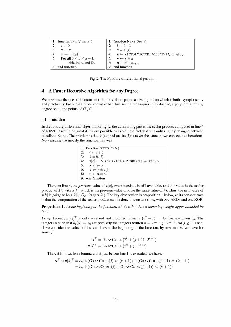
1: function INIT(f, k0,x0)2: i← 03: x← x0

4: y← f (x0)5: For all 0 ≤ k ≤ n− 1,

initialize ck and Dk

6: end function

1: function NEXT(State)2: i← i+ 13: k = b1(i)4: z← VECTORVECTORPRODUCT (Dk,x)⊕ ck5: y← y ⊕ z6: x← x⊕ ek+k0

7: end function

Fig. 2: The Folklore differential algorithm.

4 A Faster Recursive Algorithm for any Degree

We now describe one of the main contributions of this paper, a new algorithm which is both asymptoticallyand practically faster than other known exhaustive search techniques in evaluating a polynomial of anydegree on all the points of (F2)

n.

4.1 Intuition

In the folklore differential algorithm of fig. 2, the dominating part is the scalar product computed in line 4of NEXT. It would be great if it were possible to exploit the fact that x is only slightly changed betweento calls to NEXT. The problem is that k (defined on line 3) is never the same in two consecutive iterations.Now assume we modify the function this way:

1: function NEXT(State)2: i← i+ 13: k = b1(i)4: z[k]← VECTORVECTORPRODUCT (Dk,x)⊕ ck5: x[k]← x6: y← y ⊕ z[k]8: x← x⊕ ek9: end function

Then, on line 4, the previous value of z[k], when it exists, is still available, and this value is the scalarproduct ofDk with x[k] (which is the previous value of x for the same value of k). Thus, the new value ofz[k] is going to be z[k]⊕Dk · (x⊕ x[k]). The key observation is proposition 1 below, as its consequenceis that the computation of the scalar product can be done in constant time, with two ANDs and one XOR.

Proposition 1. At the beginning of the function, x> ⊕ x[k]> has a hamming weight upper-bounded bytwo.

Proof. Indeed, x[k0]> is only accessed and modified when b1(i> + 1

)= k0, for any given k0. The

integers u such that b1(u) = k0 are precisely the integers written u = 2k0 + j · 2k0+1, for j ≥ 0. Then,if we consider the values of the variables at the beginning of the function, by invariant ii, we have forsome j:

x> = GRAYCODE(2k + (j + 1) · 2k+1

)

x[k]> = GRAYCODE(2k + j · 2k+1

)

Thus, it follows from lemma 2 that just before line 1 is executed, we have:

x> ⊕ x[k]> = ek ⊕ (GRAYCODE(j) (k + 1))⊕ (GRAYCODE(j + 1) (k + 1))

= ek ⊕ ((GRAYCODE (j)⊕ GRAYCODE (j + 1)) (k + 1))

90

and by lemma 1,x> ⊕ x[k]> = ek ⊕ ek+1+b1(j+1) (4)

ut

By looking closely at the proof of proposition 1, we can write an optimized differential algorithm.However, before that, a few details still need to be addressed.

– The first time that b1(i) = k, then z[k] is not defined. In this case, we in fact know that i = 2k.Therefore, special care must be taken to initialize z[k] when b2(i) = −1, which is equivalent tosaying that the hamming weight of i is less than two. In that case, by invariant ii, we have:

x =

e0 if i = 1

ek ⊕ ek−1 if i = 2k and k > 0

– Also note that with the notation k1 = b1(i) and k2 = b2(i), then if b2(i) 6= −1, equation (4) becomes:

x⊕ x[k] = ek1 ⊕ ek2And thus,

VECTORVECTORPRODUCT(Dk1 ,x⊕ x[k1]) = Dk1 [k1]⊕Dk1 [k2]

This last formula can be further simplified by observing that Dk1 [k1] = 0.

All these considerations lead to the algorithm shown in fig. 3. Note that the conditional statementcould be removed by unrolling the loop carefully. The critical part of the algorithm is therefore an ex-tremely reduced section of the code, that performs two XORs, increment a counter, and evaluate b1 aswell as b2. The cost of maintaining i, k1 and k2 can again be reduced greatly by unrolling the loop.

1: function INIT(f, k0,x0)2: i← 03: x← x0

4: y← f(x0)5: For all 0 ≤ k ≤ n− 1,6: initialize ck and Dk

7: End for8: z[0]← c09: For all 1 ≤ k ≤ n− 1,10: z[k]← Dk[k − 1]11: End for12: end function

1: function NEXT(State)2: i← i+ 13: k1 = b1(i)4: k2 = b2(i)5: if k2 6= −1 then6: z[k1]← z[k1]⊕Dk1 [k2]7: end if8: y← y ⊕ z[k1]9: x← x⊕ ek0+k1

10: end function

Fig. 3: An optimized differential enumeration algorithm for quadratic forms.

4.2 Recursive Generalization to Any Degree.

It is in fact possible to generalize the improvement of the folklore differential algorithm that lead to theoptimized differential algorithm in the quadratic case. The core idea is that in this algorithm, a givenderivative is evaluated on the consecutive points of something that looks very much like a Gray code.This suggest using the technique recursively.

91

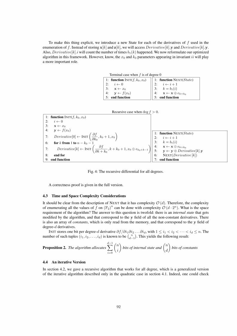
To make this thing explicit, we introduce a new State for each of the derivatives of f used in theenumeration of f . Instead of storing x[k] and z[k], we will accessDerivative[k].y andDerivative[k].y.Also,Derivative[k].iwill count the number of times b1(k) happened. We now reformulate our optimizedalgorithm in this framework. However, know, the x0 and k0 parameters appearing in invariant ii will playa more important role.

Terminal case when f is of degree 01: function INIT(f, k0, x0)2: i← 03: x← x04: y← f(x0)5: end function

1: function NEXT(State)2: i← i+ 13: k = b1(i)4: x← x⊕ ek+k0

5: end function

Recursive case when deg f > 0.1: function INIT(f, k0, x0)2: i← 03: x← x04: y← f(x0)

7: Derivative[0]← INIT

(∂f

∂k0, k0 + 1, x0

)

6: for k from 1 to n− k0 − 1

7: Derivative[k]← INIT

(∂f

∂k + k0, k + k0 + 1, x0 ⊕ ek0+k−1

)

8: end for9: end function

1: function NEXT(State)2: i← i+ 13: k = b1(i)4: x← x⊕ ek+k0

5: y← y ⊕Derivative[k].y6: NEXT(Derivative [k])7: end function

Fig. 4: The recursive differential for all degrees.

A correctness proof is given in the full version.

4.3 Time and Space Complexity Considerations

It should be clear from the description of NEXT that it has complexity O (d). Therefore, the complexityof enumerating all the values of f on (F2)

n can be done with complexity O (d · 2n). What is the spacerequirement of the algorithm? The answer to this question is twofold: there is an internal state that getsmodified by the algorithm, and that correspond to the y field of all the non-constant derivatives. Thereis also an array of constants, which is only read from the memory, and that correspond to the y field ofdegree-d derivatives.

INIT stores one bit per degree-d derivative ∂f/∂i1∂i2 . . . ∂id, with 1 ≤ i1 < i2 < · · · < id ≤ n. Thenumber of such tuples (i1, i2, . . . , id) is known to be

(nd−1). This yields the following result:

Proposition 2. The algorithm allocatesd−1∑

i=0

(n

i

)bits of internal state and

(n

d

)bits of constants

4.4 An iterative Version

In section 4.2, we gave a recursive algorithm that works for all degree, which is a generalized versionof the iterative algorithm described only in the quadratic case in section 4.1. Indeed, one could check

92

that unrolling the algorithm of fig. 4 with a quadratic f gives back the algorithm of fig. 3. We now moveon to write an iterative version of the general recursive algorithm. This iterative version allows moreoptimization, such as the removal of extra useless work, and a more careful parallel scheduling.

But first, the function NEXT2 shown in fig. 5 does exactly the same thing as NEXT, but in a slightlydifferent way. Instead of calling NEXT at the end, it calls it at the beginning, except the first time a givenvalue of k is reached, to avoid calling it an extra time at the begining.

1: function NEXT2(State)2: i← i+ 13: k = b1(i)4: if i 6= 2k then5: NEXT2 (Derivative [k])6: end if7: x← x⊕ ek+k0

8: y← y ⊕Derivative[k].y9: end function

Fig. 5: An equivalent version of NEXT.

We can therefore work on NEXT2. A first remark is that maintaining x is required by the invariants, butis otherwise useless for the actual computation. A first step is to completely remove x from the algorithm.Less obviously, we can also avoid maintaining i. To see that, we first need to state an equivalent oflemma ?? adapted to NEXT2, the proof of which is left to the reader.

Lemma 3. After k is updated on line 3 of NEXT2, we have:

i> + 1 = 2k + (Derivative[k].i+ 1)× 2k+1.

It is an easy consequence of lemma 3 that in NEXT2, after k is updated on line 3, we have for any j:

bj(Derivative[k].i+ 1) = bj+1(i> + 1).

Thus, it is possible to avoid storing the i values, except in the main loop, and to re-generate onlineby evaluating bj on the index of the main loop. These computations, although taking amortized constanttime, can be made negligible by unrolling. To ease notation, we introduce the following shorthand:

D[k1, k2, . . . , k`]∆= State.Derivative[k1].Derivative[k2] . . . .Derivative[k`].y

With this notation, the algorithm of fig. 6 is just an unrolled version of the recursive algorithm of fig. 4in which all the useless operations have been removed.

5 Enumeration of Several Multivariate Polynomials Simultaneously

In the previous section, we discussed how to enumerate one single polynomial. We now move on to theenumeration of several polynomial simultaneously.

We will use several time the following simple idea: all the techniques we discussed above perform asequence of operations that is independent of the coefficients of the polynomials. Therefore, m instancesof (say) the algorithm of fig. 6 could be run in parallel on f1, . . . , fm. All the parallel runs would execute

93

1: procedure ZEROES(f )2: State← INIT(f, 0, 0)3: for i from 0 to 2n − 14: if State.y = 0 then GRAYCODE(i) is a zero of f5: k1 = b1(i+ 1)6: k2 = b2(i+ 1)7: . . .8: kd = bd(i+ 1)9: if kd > −1 then D [k1, . . . , kd−1]← D [k1, . . . , kd−1]⊕D [k1, . . . , kd−1, kd]10: . . .11: if k3 > −1 then D [k1, k2]← D [k1, k2]⊕D [k1, k2, k3]12: if k2 > −1 then D [k1]← D [k1]⊕D [k1, k2]13: y← y ⊕D [k1]14: end for15: end procedure

Fig. 6: Iterative algorithm for all degrees.

the same instruction on different data, making it efficient to implement on vector or SIMD architectures.In each iteration of the main loop, it is easy to check if all the polynomials vanished on the current pointof (F2)

n. Evaluating all the m polynomials in parallel using the algorithm of fig. 6 would require roughlym · d · 2n bit operations. The point of this section is that it is possible to do much better than this.

Let us first introduce a useful notation. Given an ordered set U , we denote the common zeroes off1, . . . , fm belonging toU byZ([f1, . . . , fm], U). Let us also denoteZ0 = (F2)

n, andZi = Z ([fi], Zi−1).It should be clear that Z = Zm is the set of common zeroes of the polynomials, and therefore the objectwe wish to obtain.

5.1 General Technique: Splitting the Problem

A possible strategy is to compute the Zi recursively: first Z1, then Z2, etc. However, while the algorithmsof section 4 can be used to compute Z1, they cannot be used to compute Z2 from Z1, because theyintrinsically enumerate all (F2)

n. In practice, the best results are in fact obtained by computing Zk, forsome well-chosen value of k, using k parallel runs of the algorithm of fig. 6, and then computing Zmusing a secondary algorithm. Computing Zk requires d · k · 2n bit operations. It then remains to computeZm from Zk, and to find the best possible value of k.

Note that if m > n, we can focus on the first n equations, since a system of n randomly chosenmultivariate polynomial equations in n variables of constant degree d is expected to have a constantnumber of solutions, which can in turn be checked against the remaining equations efficiently. If m < n,then we can specialize m−n variables, and solve the m equations in m variables for any possible valuesof the specialized variables. All-in-all, the interesting case is when m = n.

Also note that it makes sense to choose k according to the targeted hardware platform (e.g., k = 32 ifonly 32-bit registers are available), it is an interesting theoretical problem choose k in order to minimizethe global number of bit operations.

We now move on to discuss several secondary algorithms to compute Zm from Zk, and discuss theirrelative merits.

5.2 Naive Secondary Evaluation

We compute Zi+1 from Zi using naive evaluation, for k ≤ i ≤ n − 1. It is clear that the expectedcardinality of Zi for random polynomial equations is 2n−i. We will assume for the sake of simplicity that

94

evaluating a degree-d polynomial requires(nd

), following the reasoning in section 3. Computing Zi+1

then takes about(nd

)· 2n−i bit ops. The expected cost of computing Z is then approximately:

n∑

i=k

(n

d

)· 2n−i ≈

(n

d

)· 2n−k+1 bit operations.

Minimizing the global cost means solving the equation:

k · d · 2n =

(n

d

)· 2n−k+1.

which is easily seen to be equivalent to:

(k · ln 2) · exp(k · ln 2) = 2 ·(n

d

)· ln 2d

Now, the Lambert W function is such that W (x) · exp(W (x)) = x. Thus, the solution of our equation is:

k =W

((n

d

)· 2 · ln 2

d

)/ ln 2

Using the known fact [15] that when x goes to infinity:

W (x) = lnx− ln lnx+ o(ln lnx)

we find that when n→∞:

k = 1 + log2

((n

d

)· 1d

)+O (ln lnn)

The full cost of the algorithm is then approximately d2 · log2 n · 2n+1 bit operations..

5.3 Differential Secondary Evaluation

We only describe the quadratic case, but this could be extended to higher degrees. We can efficientlyevaluate Zi+1 from Zi using an easy consequence of equation (1): given f(x), computing f(x + ∆)takes 2|∆| · n bit operations, where |∆| denote the hamming weight of ∆, by computing |∆| vector-vector products with the derivatives. Let us order the elements of Zi by writing: Zi =

xi1, . . .x

iqi

(the

elements are ordered using the usual lexicographic order), and ∆ij = xij+1 ⊕ xij .

Computing Zi+1 therefore requires approximately:

2n ·qi−1∑

j=1

|∆ij | bit operations.

Now, let us consider the ∆ij as integer number between 0 and 2n− 1. The xij+1 are the zeroes of a set

of i random polynomials, and under the assumption that each point of (F2)n has one chance over 2i to be

such a zero, then the difference ∆ij between two such consecutive zeros follows a geometric distribution

of parameter 2−i, and thus has expectation 2i. The hamming weight |∆ij | is upper-bounded by

⌈log2∆

ij

⌉

(considered as an integer), and therefore |∆ij | has expectation less than i.

Computing Zi+1 therefore requires in average 2n · i · 2n−i bit op. Finally, computing Z from Zkrequires on average:

2n ·n−1∑

i=k

i · 2n−i ≤ 4n · (k + 1) · 2n−k bit operations

95

An approximately optimal value of k would then satisfy

2k · 2n = 4n · (k + 1) · 2n−k

which is approximately k = 1 + log2 n. The complexity of the whole procedure is then 4 log2 n · 2n.However, implementing this technique efficiently looks like a lot of work for at best a 2× gain.

6 A Brief Description of the Hardware Platforms

6.1 Vector Units on x86-64

The most prevalent SIMD (single instruction, multiple data) instruction set today is SSE2, available onall current Intel-compatible CPUs. SSE2 instructions operate on 16 architectural xmm registers, each ofwhich is 128-bit wide. We use integer operations, which treat xmm registers as vectors of 8-, 16-, 32- or64-bit operands.

The highly non-orthogonal SSE instruction set includes Loads and Stores (to/from xmm registers,memory — both aligned and unaligned, and traditional registers), Packing/Unpacking/Shuffling, LogicalOperations (AND, OR, NOT, XOR, Shifts Left, Right Logical and Arithmetic — bit-wise on units andbyte-wise on the entire xmm register), and Arithmetic (add, substract, multiply, max-min) with some orall of the arithmetic widths. The interested reader is referred to Intel and AMD’s manuals for details onthese instructions, and to references such as [19] for throughput and latencies.

6.2 G2xx-series Graphics Processing Units from NVIDIA

We choose NVIDIA’s G2xx GPUs as they have the least hostile GPU parallel programming environmentcalled CUDA (Compute Unified Device Architecture). In CUDA, we program in the familiar C/C++programming language plus a small set of GPU extensions.

An NVIDIA GPU contains anywhere from 2–30 streaming multiprocessors (MPs). There are 8 ALUs(streaming processors or SPs in market-speak) and two super function units (SFUs) on each MP. A top-end “GTX 295” card has two GPUs, each with 30 MPs, hence the claimed “480 cores”. The theoreticalthroughput of each SP per cycle is one 32-bit integer or floating-point instruction (including add/subtract,multiply, bitwise AND/OR/XOR, and fused multiply-add), and that of an SFU 2 floating-point multipli-cations or 1 special operation. The arithmetic units have 20+-stage pipelines.

Main memory is slow and forms a major bottleneck in many applications. The read bandwidth frommemory on the card to the GPU is only one 32-bit read per cycle per MP and has a latency of > 200cycles. To ease this problem, the MP has a register file of 64 KB (16,384 registers, max. of 128 perthread), a 16-bank shared memory of 16 KB, and an 8-KB cache for read-only access to a declared“constant region” of at most 64 KB. Every cycle, each MP can achieve one read from the constant cache,which can broadcast to many thread at once.

Each MP contains a scheduling and dispatching unit that can handle a large number of lightweightthreads. However, the decoding unit can only decode once every 4 cycles. This is typically 1 instruction,but certain common instructions are “half-sized”, so two such instructions can be issued together ifindependent. Since there are 8 SPs in an MP, CUDA programming is always on a Single Program MultipleData basis, where a “warp” of threads (32) should be executing the same instruction. If there is a branchwhich is taken by some thread in a warp but not others, we are said to have a “divergent” warp; from thenon only part of the threads will execute until all threads in that warp are executing the same instructionagain. Further, as the latency of a typical instruction is about 24 cycles, NVIDIA recommends a minimumof 6 warps on each MP, although it is sometimes possible to get acceptable performance with 4 warps.

96

7 Parallelization and Memory Bandwith Issues

The critical loop of the algorithm is very short, since it performs only d logical operations. However, itaccesses the memory d+1 times, which suggests that the memory bandwith will be the actual performancebottleneck. We address this issue in two complementary ways. First we argue that the algorithm is cache-oblivious [20], i.e., that is uses the cache efficiently regardless of its size. Then we argue that on massivelyconcurrent architectures such as GPUs, then any word read from the memory can be broadcast to all theconcurrently running threads almost systematically.

7.1 Spatial and Temporal Proximity on Iterative Architectures

We will study the behavior of the algorithm in the Ideal Cache Model. This model consists of a computerwith a two-level memory hierarchy consisting of an ideal (data) cache of Z words and an arbitrarily largemain memory. The cache is partitioned into cache lines, each consisting of L consecutive words that arealways moved together between cache and main memory. The processor can only reference words thatreside in the cache. If the referenced word belongs to a line already in cache, a cache hit occurs, andthe word is delivered to the processor. Otherwise, a cache miss occurs, and the line is fetched into thecache. The ideal cache is fully associative: cache lines can be stored anywhere in the cache. If the cacheis full, a cache line must be evicted. The ideal cache uses the optimal off-line strategy of replacing thecache line whose next access is farthest in the future, and thus it exploits temporal locality perfectly. Analgorithm with an input of size n is measured in the ideal-cache model in terms of the usual number ofoperation performed by the processor, but also in terms of its Cache Complexity Q(n,Z, L) – the numberof cache misses it incurs as a function of Z and L. We now move on to evaluate the cache complexityof the enumeration algorithm, as show in fig. 6. We will assume that the “memory cells” accessed by thealgorithm have the same size as the a word in the cache (if this were not the case, it would only incur aconstant multiplicative loss, and we are mostly interested in an asymptotic result).

The memory words accessed in the algorithm belong to arrays of various dimension, and are accessedwith indices of variable length. It should be clear from the description of the algorithm that for all k ≤ d,the memory location of index [i1, . . . , ik] is accessed at step s if bj(s) = ij , for all j ≤ k. This memoryaccess pattern is in fact very regular. We say that a memory word is accessed with period T if, when it isaccessed at iteration i, it is also accessed at iteration i+ T , but not in-between.

Lemma 4. For all k ≤ d, the memory location of index [i1, . . . , ik] is accessed with period 2ik+1.

Proof. We associate with an index [i1, . . . , ik] the setΩi1,...,ik of integers n such that b1(n) = i1, . . . , bk(n) =ik. The problem amounts to show that the difference between two consecutive elements of this set is2ik+1. But it is easily seen that if n ∈ Ωi1,...,ik , then n+ j · 2ik+1 ∈ Ωi1,...,ik for any positive integer j.This follows from the fact that bj(n) = bj(n+ 2`) if ` > j, and establishes the result. ut

It should be clear that all the memory location accessed with period exactly T are accessed in thefirst T iteration of the main loop. Moreover, they are accessed in a certain order. For instance, memorywords with period 8 are accessed in this order in the first 8 iterations: [2], [0, 2], [1, 2]. By definition ofthe period, this access pattern is reproduced without modifications in the next T iterations. Thus, memorywords with period T are accessed in a cyclic fashion.

The algorithm easily defines a total order relation on the memory locations it accesses: x ≤ y if andonly if the first access to x takes places before the first access to y. Let us assume that the actual memoryaddresses are compatible with this order relation. Then, more frequently accessed words are stored withthe lowest addresses, and words with the same access frequency are stored contiguously in memory. Thereare∑min(d−1,k)i=0

(ki

)memory locations that are accessed with period 2k+1.

97

This being said, we will focus on the case where all the∑di=0

(ni

)memory words accessed by the

algorithm do not fit into the cache, to avoid studying the trivial case. Let us define the critical period2Tc+1 to be the biggest integer such that all the memory words accessed with period 2Tc+1 fit in thecache:

Tc∑

k=0

min(d−1,k)∑

i=0

(k

i

)≤ Z − 1

Under the (mild) assumption that the cache contains Z ≥ 2d words, and thus that Tc is greater than d,this condition becomes:

2d − 1 +

Tc∑

k=d

d−1∑

i=0

(k

i

)≤ Z − 1

This this is the summation in a rectangle inside Pascal’s triangle, then by applying Pascal’s rule recur-sively, we may simplify this expression, and find that it is equivalent to:

d∑

i=0

(Tc + 1

i

)≤ Z

The important point is that all memory words with period 2Tc+1 fit in the cache and do not leave it.This fact is almost true by definition of Tc: the optimal off-line cache strategy will not evict a cache linethat will be accessed in T steps if it can evict a cache line that will only be accessed in 2T steps. Andthere will always be a cache line not containing a word accessed with period 2Tc+1 or less. This beingsaid, we can state our result:

Proposition 3. Under the assumption that Tc ≥ 2d, the following two inequalities hold:

i) Q(n, d, Z, L) ≤ 2n−2−Tc · (d+ 1) ·(Tc + 1

d− 1

)

ii) Q(n, d, Z, L) ≤ 2n−2−Tc · d · (d+ 1)

Tc + 2− d · Z

The proof is in the full version of the paper.Let us consider a polynomial in 64 variables. If we assume an incredibly small cache of Z = 210 bits

and that our polynomial is of degree 2, then Tc = 44 and the enumeration will make about 225 cachemisses, for a running time of at least 265. If we assume that our polynomial is of degree 4, and that thecache is 214-bit large, then Tc = 24, and there will be 252 cache misses, for more than 266 memoryaccesses.

7.2 Constrained Small Memory Chips on Concurrent Architectures

The problem is formulated in very different terms on some parallel architectures, such as GPUs, or theCell, in which the available “fast” memory is fairly restricted, and main memory is relatively slow.

Parallelizing the process is very easy, as it simply comes down to partition the search space into thenumber of available cores. An interesting side effect is that when done properly, this partition reducesthe amount of data that needs to be transfered from the main memory. We will now assume that we have32-bit registers, and we will use 32 parallel copies of the algorithm of fig. 6, to enumerate 32 polynomialssimultaneously.

For instance, the loop of fig. 4 can be split in independent chunks, as illustrated by fig. 7. An additionalbenefit is that processing one such chunk only require access to a fraction of the memory used by the fullenumeration. In fact, b1(i + 1) is greater or equal than L if the L rightmost bits of (i + 1) are zero, or,

98

in other terms, if (i + 1) is a multiple of 2L. This suggests to split the iteration in chunks of size 2L.Enumerating a chunk of size 2L amounts to enumerate a polynomial in L variables (it requires the sameamount of internal state, and it makes the same number of calls to NEXT). Let us now consider the k-thchunk:

Ck =i ∈ N | k · 2L < i ≤ (k + 1) · 2L

1: procedure PARALLELZEROES(f, L, T )2: for b from 0 to 2n−L−T − 1 do2: parallel-for t from 0 to 2T − 1 do3: State[t]← INIT

(f, 0,GRAYCODE

((t+ b · 2T

)· 2L

))

2: for i from 0 to 2L − 1 do4: if State[t].y = 0 then State[t].x is a zero of f5: NEXT(State[t])6: end for7: end-parallel for6: end for8: end procedure

Fig. 7: Parallel enumeration, assuming one processing unit capable of running 2T threads. It should bepossible to improve it using the enumeration algorithm itself for initialization.

Let ψL(i) denote the integer (i mod 2L). We will call ψL(i) the local part of i when i ∈ Ck, and wewill denote it by ψ(i), when not ambiguous. So, what can we say about bj(i), when i ∈ Ck? We definethe subset Ωk,j of Ck to be such that if i ∈ Ωk,j , then bj(i) only depends on the local part ψ(i) of i. Veryclearly, we in fact have:

Ωk,j =i ∈ Ck | HAMMINGWEIGHT(ψ(i)) ≥ j

And the three following points are immediate to estalbish.

Lemma 5. For any k and j, we have the following properties:

i) If j1 < j2 then Ωk,j2 ⊆ Ωk,j1

ii) |Ωk,j | = 2L −j−1∑

`=0

(L

`

)

iii) If i ∈ Ωk,j , then bj(i) < L.

Intuitively, lemma 5 tells us that on a chunk of size 2L, the bj that we will compute will be smallerthan L except on O

(Ld−1

)points, and will only depend on the local part of the index. This has two

interesting consequences:

1. Instead of having to store and maintain an internal state of∑d−1i=0

(ni

)= O

(nd−1

)words, it is

sufficient to deal with an internal state of∑d−1i=0

(Li

)= O

(Ld−1

)words.

2. If we were capable of processing all the chunks synchronously, the constant fetched from memoryin line 9 of fig. 6 could be used by all the chunks at the same time, except on O

(Ld−1

)points. This

means that most of the time, we can broadcast a single value to as many threads as possible, and wecan amortize the lattency of the memory over the huge number of chunks processed in parallel.

99

Now that we controlled what happened inside Ωk,d, we may take a look at what happens outside. Gener-ally speaking, if ψ(i) has hamming weight h, and j > h, then bj(i) = L+bj−h(k). Thus, if only a subsetof all the chunks can be processed concurrently, it would make sense to treat simultaneously chunks forwhich k has similar least-significant bits. If a processing unit can handle at most 2T threads simultane-ously, then the maximum sharing of values fetched from main memory is achieved by scheduling the 2T

Chunks sharing the T most significant bit of k on it.What level of broadcast should we expect in this situation, namely when 2t threads process chunks of

size 2L synchronously? To fully understand what is going on, let us define Hk,h = Ωk,h − Ωk,h+1. It iseasily seen that Hk,h describes the subset of Ck formed of words of hamming weight exactly h, and thus|Hh,k| =

(Lh

). Now, in all the chunks processed in parallel, the c = n − L − t least significant bits of

k remain fixed to ψc(k), therefore we will call this value the “fixed part of k”. We already argued that ifi ∈ Hh,k, then bj(i) = L+ bj−h(k), and the 2T threads will fetch the same memory location if and onlyif bj−h(k) only depends on the fixed part of k, or, in other terms, if ψc(k) has hamming weight at leastj − h.

An easy consequence of the previous considerations is that if ψc(k) has hamming weight at least d,then all the memory fetches issued on the 2L steps can be broadcast to all the 2T threads. If ψc(k) hashamming weight d− 1, then all but one memory fetches can be broadcast.

This raises the following question: assume we enumerate the 2n points on a processing unit han-dling 2T concurrent threads, each thread processing a chunk of size 2L (we of course assume n ≥L+T ). How many times we will witness non-broadcast memory accesses? Let us denote this number byNNB(d, n, T, L).

Proposition 4.

NNB(d, n, T, L) =d−1∑

i=0

(n− Ti

).

The proof is in the full version.Fig. 8 shows how the algorithm can be run with 4 threads and obtain the number of non-broadcasts

advertised by the proposition.

8 Implementations

We describe the structure of our code, the approximate cost structure, our design choices and justify whatwe did. Our implementation code always consists of three stages:

Partial Evaluation: We substitute all possible values for s variables (xn−s, . . . , xn−1) out of n, thussplitting the original system into 2s smaller systems, of w equations each in the remaining (n − s)variables (x0, . . . , xn−s−1), and output them in a form that is suitable for ...

Enumeration Kernel: Run the algorithm of Sec. 4 to find all candidate vectors x satisfying w equationsout of m (≈ 2n−w of them), which are handed over to ...

Candidate Checking: Checking possible solutions x in remaining m− w equations.

8.1 CPU Enumeration Kernel

Typical code fragments from the unrolled inner loops can be seen below:

100

thread 0 thread 1 thread 2 thread 3k ψL(i) b1(i) b2(i) k ψL(i) b1(i) b2(i) k ψL(i) b1(i) b2(i) k ψL(i) b1(i) b2(i) non-broadcast ?0 1 0 -1 100 1 0 5 1000 1 0 6 1100 1 0 5 D

0 10 1 -1 100 10 1 5 1000 10 1 6 1100 10 1 5 D

0 11 0 1 100 11 0 1 1000 11 0 1 1100 11 0 10 100 2 -1 100 100 2 5 1000 100 2 6 1100 100 2 5 D

0 101 0 2 100 101 0 2 1000 101 0 2 1100 101 0 20 110 1 2 100 110 1 2 1000 110 1 2 1100 110 1 20 111 0 1 100 111 0 1 1000 111 0 1 1100 111 0 10 0 3 -1 100 0 3 5 1000 0 3 6 1100 0 3 5 D

1 1 0 3 101 1 0 3 1001 1 0 3 1101 1 0 31 10 1 3 101 10 1 3 1001 10 1 3 1101 10 1 31 11 0 1 101 11 0 1 1001 11 0 1 1101 11 0 11 100 2 3 101 100 2 3 1001 100 2 3 1101 100 2 31 101 0 2 101 101 0 2 1001 101 0 2 1101 101 0 21 110 1 2 101 110 1 2 1001 110 1 2 1101 110 1 21 111 0 1 101 111 0 1 1001 111 0 1 1101 111 0 11 0 4 -1 101 0 4 5 1001 0 4 6 1101 0 4 5 D

10 1 0 4 110 1 0 4 1010 1 0 4 1110 1 0 410 10 1 4 110 10 1 4 1010 10 1 4 1110 10 1 410 11 0 1 110 11 0 1 1010 11 0 1 1110 11 0 110 100 2 4 110 100 2 4 1010 100 2 4 1110 100 2 410 101 0 2 110 101 0 2 1010 101 0 2 1110 101 0 210 110 1 2 110 110 1 2 1010 110 1 2 1110 110 1 210 111 0 1 110 111 0 1 1010 111 0 1 1110 111 0 110 0 3 4 110 0 3 4 1010 0 3 4 1110 0 3 411 1 0 3 111 1 0 3 1011 1 0 3 1111 1 0 311 10 1 3 111 10 1 3 1011 10 1 3 1111 10 1 311 11 0 1 111 11 0 1 1011 11 0 1 1111 11 0 111 100 2 3 111 100 2 3 1011 100 2 3 1111 100 2 311 101 0 2 111 101 0 2 1011 101 0 2 1111 101 0 211 110 1 2 111 110 1 2 1011 110 1 2 1111 110 1 211 111 0 1 111 111 0 1 1011 111 0 1 1111 111 0 111 0 5 -1 111 0 6 -1 1011 0 5 6 1111 0 7 -1 D

Fig. 8: Enumeration with n = 7, in chunks of 23 elements with 4 batches of 4 concurrent threads. “Non-local” means that a constant of index greater than 3 is accessed, while “Non-broadcast” means that the 4threads do not access the same memory location. In conformance with lemma 4, there are 1 + 7− 2 = 6non-broadcast memory accesses.

101

(a) quadratics, C++ x86 instrinsics (b) quadratics, x86 assembly...diff0 ^= deg2_block[ 1 ];res ^= diff0;Mask = _mm_cmpeq_epi16(res, zero);mask = _mm_movemask_epi8(Mask);if(mask) check(mask, idx, x^155);...

.L746:movq 976(%rsp), %rax //pxor (%rax), %xmm2 // d_y ^= C_yzpxor %xmm2, %xmm1 // res ^= d_ypxor %xmm0, %xmm0 //pcmpeqw %xmm1, %xmm0 // cmp words for eqpmovmskb %xmm0, %eax // movemasktestw %ax, %ax // set flag for branchjne .L1266 // if needed, check and

.L747: // comes back here

.L1624:movq 2616(%rsp), %rax // load C_yzamovdqa 2976(%rsp), %xmm0 // load d_yzpxor (%rax), %xmm0 // d_yz ^= C_yzamovdqa %xmm0, 2976(%rsp) // save d_yzpxor 8176(%rsp), %xmm0 // d_y ^= d_yzpxor %xmm0, %xmm1 // res ^= d_ymovdqa %xmm0, 8176(%rsp) // save d_ypxor %xmm0, %xmm0 //pcmpeqw %xmm1, %xmm0 // cmp words for eqpmovmskb %xmm0, %eaxtestw %ax, %ax // ...jne .L2246 // branch to check

.L1625: // and comes back

...diff[0] ^= deg3_ptr1[0];diff[325] ^= diff[0];res ^= diff[325];Mask = _mm_cmpeq_epi16(res, zero);mask = _mm_movemask_epi8(Mask);if(mask) check(mask, idx, x^2);...

(c) cubics, x86 assembly (d) cubics, C++ x86 instrinsics

testing All zeroes in one byte, word, or dword in a XMM register can be tested cheaply on x86-64. Wehence wrote code to test 16 or 32 equations at a time. Strangely enough, even though the code above isfor 16 bits, the code for checking 32/8 bits at the same time is nearly identical, the only difference beingthat we would subtitute the intrinsics _mm_cmpeq_epi32/8 for _mm_cmpeq_epi16 (leading to theSSE2 instruction pcmpeqd/b instead of pcmpeqw). Whenever one of the words (or double words orbytes, if using another testing width) is non-zero, the program branches away and queues the candidatesolution for checking.

unrolling One common aspect of our CPU and GPU code is deep unrolling by upwards of 1024× toavoid the expensive bit-position indexing. To illustrate with quartics as an example, instead of having tocompute the positions of the four rightmost non-zero bits in every integer, we only need to compute thefirst four rightmost non-zero bits in bit 10 or above, then fill in a few blanks. This avoids most of theindexing calculations and all the calculations involving the most commonly used differentials.

We wrote similar Python scripts to generate unrolled loops in C and CUDA code. Unrolling is evenmore critical with GPU, since divergent branching and memory accesses are prohibitively expensive.

8.2 GPU Enumeration Kernel

register usage Fast memory is precious on GPU and register usage critical for CUDA programmers. Ouralgorithms’ memory complexity grows exponentially with the degree d, which is a serious problem whenimplementing the algorithm for cubic and quartic systems, compounded by the immaturity of NVIDIA’snvcc compiler which tends to allocate more registers than we expected.

Take quartic systems as an example. Recall that each thread needs to maintain third derivatives, whichwe may call dijk for 0 ≤ i < j < k < K, where K is the number of variables in each small system. ForK = 10, there are 120 dijk’s and we cannot waste all our registers on them, especially as all differentialsare not equal — dijk is accessed with probability 2−(k+1).

Our strategy for register use is simple: Pick a suitable bound u, and among third differentials dijk(and first and second differentials di and dij), put the most frequently used — i.e., all indices less than u— in registers, and the rest in device memory (which can be read every 8 instructions without choking).We can then control the number of registers used and find the best u empirically.

102

fast conditional move We discovered during implementation an undocumented feature of CUDA forG2xx series GPUs, namely that nvcc reliably generates conditional (predicated) move instructions, dis-patched with exceptional adeptness....xor.b32 $r19, $r19, c0[0x000c] // d_y^=d_yzxor.b32 $p1|$r20, $r17, $r20mov.b32 $r3, $r1mov.b32 $r1, s[$ofs1+0x0038]xor.b32 $r4, $r4, c0[0x0010]xor.b32 $p0|$r20, $r19, $r20 // res^=d_y@$p1.eq mov.b32 $r3, $r1@$p1.eq mov.b32 $r1, s[$ofs1+0x003c]xor.b32 $r19, $r19, c0[0x0000]xor.b32 $p1|$r20, $r4, $r20@$p0.eq mov.b32 $r3, $r1 // cmov@$p0.eq mov.b32 $r1, s[$ofs1+0x0040] // cmov...

...diff0 ^= deg2_block[ 3 ]; // d_y^=d_yzres ^= diff0; // res^=d_yif( res == 0 ) y = z; // cmovif( res == 0 ) z = code233; // cmovdiff1 ^= deg2_block[ 4 ];res ^= diff1;if( res == 0 ) y = z;if( res == 0 ) z = code234;diff0 ^= deg2_block[ 0 ];res ^= diff0;if( res == 0 ) y = z;if( res == 0 ) z = code235;...

(a) decuda result from cubin (b) CUDA code for a inner loop fragmentConsider, for example, the code displayed above right. According to our experimental results, the

repetitive 4-line code segments average less than three SP (stream-processor) cycles. However, decudaoutput of our program shows that each such code segment corresponds to at least 4 instructions including2 XORs and 2 conditional moves [as marked in above left]. The only explanation is that conditionalmoves can be dispatched by the SFUs (Special Function Units) so that the total throughput can exceed1 instruction per SP cycle. Further note that the annotated segment on the right corresponds to actualinstructions far apart because an NVIDIA GPU does opportunistic dispatching but is nevertheless a purelyin-order architecture, so proper scheduling must interleave instructions from different parts of the code.

testing The inner loop for GPUs differs from CPUs due to the fast conditional moves.Here we evaluate 32 equations at a time using Gray code. The result is used to set a flag if it happens

to be all zeroes. We can now conditional move of the index based on the flag to a register variable z, andat the end of the loop write z out to global memory.

However, how can we tell if there are too many (here, two) candidate solutions in one small subsys-tem? Our answer to that is to use a buffer register variable y and a second conditional move using thesame flag. At the end of the thread, (y, z) is written out to a specific location in device memory and sentback to the CPU.

Now subsystems which have all zero constant terms are automatically satisfied by the vector of zeroes.Hence we note them down during the partial evaluation phase include the zeros with the list of candidatesolutions to be checked, and never have to worry about for all-zero candidate solution. The CPU readsthe two doublewords corresponding to y and z for each thread, and:

1. z==0 means no candidate solutions,2. z!=0 but y==0 means exactly one candidate solution, and3. y!=0 means 2+ candidate solutions (necessitating a re-check).

8.3 Checking Candidates

Checking candidate solutions is always done on CPU because the programming involves branching andhence is difficult on a GPU even with that available. However, the checking code for CPU enumerationand GPU enumeration is different.

CPU With the CPU, the check code receives a list of candidate solutions. Today the maximum machineoperation is 128-bit wide. Therefore we should collect solutions into groups of 128 possible solutions.We would rearrange 128 inputs of n bits such that they appear as n __int128’s, then evaluate onepolynomial for 128 results in parallel using 128-bit wide ANDs and XORs. After we finish all candidates

103

for one equation, go through the results and discard candidates that are no longer possible. Repeat theresult for the second and any further equations (cf. Sec. 3).

We need to transpose a bit-matrix to achieve the effect of a block of w inputs n-bit long each, ton machine-words of w-bit long. This looks costly, however, there is an SSE2 instruction PMOVMSKB(packed-move-mask-bytes) that packs the top bit of each byte in an XMM register into a 16-bit general-purpose register with 1 cycle throughput. We combine this with simultaneous shifts of bytes in an XMMand can, for example, on a K10+ transpose a 128-batch of 32-bit vectors (0.5kB total) into 32 __int128’sin about 800 cycles, or an overhead of 6.25 cycles per 32-bit vector. In general the transposition cost is atmost a few cycles per byte of data, negligible for large systems.

GPU As explained above, for the GPU we receive a list with 3 kinds of entries:

1. The knowledge that there are two or more candidate solutions within that same small system, withonly the position of the last one in the Gray code order recorded.

2. A candidate solution (and no other within the same small system).3. Marks to subsystems that have all zero constant terms.

For Case 1, we take the same small system that was passed into the GPU and run the Enumerative Kernelsubroutine in the CPU code and find all possible small systems. Since most of the time, there are exactlytwo candidate solutions, we expected the Gray code enumeration to go two-thirds of the way throughthe subsystem. Merge remaining candidate solutions with those of Case 2+3, collate for checking in alarger subsystem if needed, and pass off to the same routine as used in the CPU above. Not unexpectedly,the runtime is dominated by the thread-check case, since those does millions of cycles for two candidatesolutions (most of the time).

8.4 Partial Evaluation

The algorithm for Partial Evaluation is for the most part the same Gray Code algorithm as used in theEnumeration Kernel. Also the highest degree coefficients remain constant, need no evaluation and andcan be shared across the entire Enumeration Kernel stage. As has been mentioned in the GPU description,these will be stored in the constant memory, which is reasonably cached on NVIDIA CUDA cards. Theother coefficients can be computed by Gray code enumeration, so for example for quadratics we have(n− s) + 2 XOR per w bit-operations and per substitution. In all, the cost of the Partial Evaluation stagefor w′ equations is ∼ 2s w

′

8

((n−sd−1)+ (smaller terms)

)byte memory writes. The only difference in the

code to the Enumerative Kernel is we write out the result (smaller systems) to a buffer, and check for azero constant term only (to find all-zero candidate solutions).

Peculiarities of GPUS Many warps of threads are required for GPUs to run at full speed, hence we mustsplit a kernel into many threads, the initial state of each small system being provided by Partial Evaluation.In fact, for larger systems on GPUs, we do two stages of partial evaluation because

1. there is a limit to how many threads can be spawned, and how many small systems the device memorycan hold, which bounds how small we can split; but

2. increasing s decreases the fast memory pressure; and3. a small systems reporting two or more candidate solutions is costly, yet we can’t run a batch check

on a small system with only one candidate solution — hence, an intermediate partial evaluation sowe can batch check with fewer variables.

8.5 More Test Data and Discussion

Some minor points which the reader might find useful in understanding the test data, a full set of whichwill appear in the extended version.

104

Candidate Checking. The check code is now 6–10% of the runtime. In theory (cf. Sec. 3) evaluationshould start with a script which hard-wires a system of equations into C and compiling to an excutable,eliminating half of the terms, and leading to

(n−sd

)SSE2 (half XORs and half ANDs) operations to check

one equation forw = 128 inputs. The check code can potentially become more than an order of magnitudefaster. We do not (yet) do so presently, because compiling may take more time than the checking code.However, we may want to go this route for even larger systems, as the overhead from testing for zero bits,re-collating the results, and wasting due to the number of candidate solutions is not divisible by w wouldall go down proportionally.

Without hard-wiring, the running time of the candidate check is dominated by loading coefficients.E.g., for quartics with 44 variables, 14 pre-evaluated, K10+ and Ci7 averages 4300 and 3300 cyclesrespectively per candidate. With each candidate averaging 2 equations of

(44−14

4

)terms each, the 128-

wide inner loop averages about 10 and 7.7 cycles respectively per term to accomplish 1 PXOR and 1PAND.

Partial Evaluation. We point out that Partial Evaluation also reduces the complexity of the Checkingphase. The simplified description in Sec. 5 implies the cost of checking each candidate solution to be≈ 1

w

(nd

)instructions. But we can get down to ≈ 1

w

(n−sd

)instructions by partially evaluating w′ > w

equations and storing the result for checking. For example, when solving a quartic system with n =48, m = 64, the best CPU results are s = 18, and we cut the complexity of the checking phase by factorof at least 4× even if it was not the theoretical 7× (i.e.,

(nd

)/(n−sd

)) due to overheads.

The Probability of Thread-Checking for GPUs. If we have n variables, pre-evaluate s, and check wequations via Gray Code, then the probability of a subsystem with 2n−s vectors including at least twocandidates ≈

(2n−s

2

)(1− 2−w)2

n−s

(2−w)2 ≈ 1/22(s+w−n)+1, provided that n < s+w. As an example,for n = 48, s = 22, w = 32, the thread-recheck probability is about 1 in 213, and we must re-checkabout 29 threads using Gray Code. This pushes up the optimal s for GPUs.

Architecture and Differences. All our tests with a huge variety of machines and video cards show that thekernel time in cycles per attempt is almost a constant of the architecture, and the speed-up in multi-cores isalmost completely linear for almost all modern hardware. So we can compute the time complexity giventhe architecture, the frequency, the number of cores, and n. The marked cycle count difference betweenIntel and AMD cores is explained by Intel dispatching three XMM (SSE2) logical instructions to AMD’stwo per cycle and handling branch prediction and caching better.

As the Degree d increases. We plot how many cycles is taken by the inner loop (which is 8 vectors percore for CPUs and 1 vector per SP for GPUs) on different architectures in Fig. 9. As we can see, allexcept two architectures have inner loop cycle counts that are increasing roughly linearly with the degree.The exceptions are the AMD K10 and NVIDIA G200 architectures, which is in line with fast memorypressure on the NVIDIA GPUs and fact that K10 has the least cache among the CPU architectures.

More Tuning. We can conduct a Gaussian elimination among them equations and such thatm/2 selectedterms in m/2 of the equations are all zero. We can of course make this the most commonly used coeffi-cients (i.e., c01, c02, c12, . . . for the quadratic case). The corresponding XOR instructions can be removedfrom the code by our code generator. This is not yet automated and we have to test everything by hand.However, this clearly leads to significant savings. On GPUs, we have a speed up of 21% on quadraticcases, 18% for cubics, and 4% for quadratics. [The last is again due to the memory problems.]

Notes and Acknowledgements

C. Bouillaguet thanks Jean Vuillemin for helpful discussions. The Taiwanese authors thank Ming-ShingChen for assistance with programming and fruitful discussion, Taiwan’s National Science Council for

105

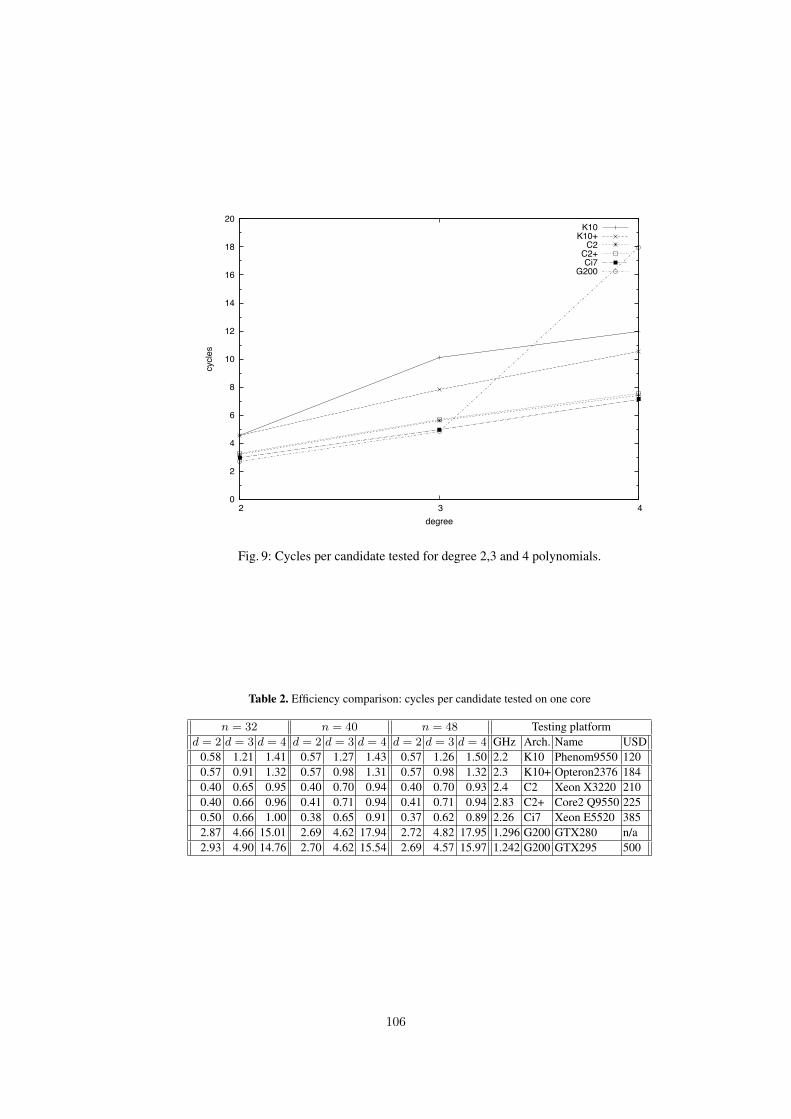
0

2

4

6

8

10

12

14

16

18

20

2 3 4

cycle

s

degree

K10K10+

C2C2+Ci7

G200

Fig. 9: Cycles per candidate tested for degree 2,3 and 4 polynomials.

Table 2. Efficiency comparison: cycles per candidate tested on one core

n = 32 n = 40 n = 48 Testing platformd = 2 d = 3 d = 4 d = 2 d = 3 d = 4 d = 2 d = 3 d = 4 GHz Arch. Name USD

0.58 1.21 1.41 0.57 1.27 1.43 0.57 1.26 1.50 2.2 K10 Phenom9550 1200.57 0.91 1.32 0.57 0.98 1.31 0.57 0.98 1.32 2.3 K10+ Opteron2376 1840.40 0.65 0.95 0.40 0.70 0.94 0.40 0.70 0.93 2.4 C2 Xeon X3220 2100.40 0.66 0.96 0.41 0.71 0.94 0.41 0.71 0.94 2.83 C2+ Core2 Q9550 2250.50 0.66 1.00 0.38 0.65 0.91 0.37 0.62 0.89 2.26 Ci7 Xeon E5520 3852.87 4.66 15.01 2.69 4.62 17.94 2.72 4.82 17.95 1.296 G200 GTX280 n/a2.93 4.90 14.76 2.70 4.62 15.54 2.69 4.57 15.97 1.242 G200 GTX295 500

106

partial sponsorship under grants NSC96-2221-E-001-031-MY3, 98-2915-I-001-041, and 98-2219-E-011-001 (Taiwan Information Security Center), and Academia Sinica for the Career Development Award.Questions and esp. corrections about the extended version should be addressed to [email protected].

References

1. G. V. Bard, N. T. Courtois, and C. Jefferson. Efficient methods for conversion and solution of sparse systemsof low-degree multivariate polynomials over gf(2) via sat-solvers. Cryptology ePrint Archive, Report 2007/024,2007. http://eprint.iacr.org/.

2. M. Bardet, J.-C. Faugère, and B. Salvy. On the complexity of Gröbner basis computation of semi-regular overde-termined algebraic equations. In Proceedings of the International Conference on Polynomial System Solving,pages 71–74, 2004. Previously INRIA report RR-5049.

3. M. Bardet, J.-C. Faugère, B. Salvy, and B.-Y. Yang. Asymptotic expansion of the degree of regularity for semi-regular systems of equations. In P. Gianni, editor, MEGA 2005 Sardinia (Italy), 2005.

4. A. T. Benjamin and J. Quinn. Proofs that Really Count: The Art of Combinatorial Proof (Dolciani MathematicalExpositions). The Mathematical Association of America, August 2003.

5. C. Berbain, H. Gilbert, and J. Patarin. QUAD: A practical stream cipher with provable security. In S. Vaudenay,editor, EUROCRYPT, volume 4004 of Lecture Notes in Computer Science, pages 109–128. Springer, 2006.

6. D. J. Bernstein, T.-R. Chen, C.-M. Cheng, T. Lange, and B.-Y. Yang. ECM on graphics cards. In A. Joux,editor, EUROCRYPT, volume 5479 of Lecture Notes in Computer Science, pages 483–501. Springer, 2009.http://eprint.iacr.org/2008/480/.

7. L. Bettale, J.-C. Faugère, and L. Perret. Hybrid approach for solving multivariate systems over finite fields.Journal of Mathematical Cryptology, 3:177–197, 2009.

8. C. Bouillaguet, J.-C. Faugère, P.-A. Fouque, and L. Perret. Differential-algebraic algorithms for the isomorphismof polynomials problem. Cryptology ePrint Archive, Report 2009/583, 2009. http://eprint.iacr.org/.

9. C. Bouillaguet, P.-A. Fouque, A. Joux, and J. Treger. A family of weak keys in hfe (and the correspondingpractical key-recovery). Cryptology ePrint Archive, Report 2009/619, 2009. http://eprint.iacr.org/.

10. B. Buchberger. Ein Algorithmus zum Auffinden der Basiselemente des Restklassenringes nach einem nulldimen-sionalen Polynomideal. PhD thesis, Innsbruck, 1965.

11. J. Buchmann, D. Cabarcas, J. Ding, and M. S. E. Mohamed. Flexible partial enlargement to accelerate gröbnerbasis computation over 2. In D. J. Bernstein and T. Lange, editors, AFRICACRYPT, volume 6055 of LectureNotes in Computer Science, pages 69–81. Springer, 2010.

12. N. Courtois, G. V. Bard, and D. Wagner. Algebraic and slide attacks on keeloq. In K. Nyberg, editor, FSE,volume 5086 of Lecture Notes in Computer Science, pages 97–115. Springer, 2008.

13. N. Courtois, L. Goubin, and J. Patarin. SFLASH: Primitive specification (second revised version), 2002. https://www.cosic.esat.kuleuven.be/nessie, Submissions, Sflash, 11 pages.

14. N. T. Courtois, A. Klimov, J. Patarin, and A. Shamir. Efficient algorithms for solving overdefined systems ofmultivariate polynomial equations. In Advances in Cryptology — EUROCRYPT 2000, volume 1807 of LectureNotes in Computer Science, pages 392–407. Bart Preneel, ed., Springer, 2000. Extended Version: http://www.minrank.org/xlfull.pdf.

15. N. de Bruijn. Asymptotic methods in analysis. 2nd edition. Bibliotheca Mathematica. Vol. 4. Groningen: P.Noordhoff Ltd. XII, 200 p. , 1961.

16. J.-C. Faugère. A new efficient algorithm for computing Gröbner bases (F4). Journal of Pure and AppliedAlgebra, 139:61–88, June 1999.

17. J.-C. Faugère. A new efficient algorithm for computing Gröbner bases without reduction to zero (F5). InInternational Symposium on Symbolic and Algebraic Computation — ISSAC 2002, pages 75–83. ACM Press,July 2002.

18. J.-C. Faugère and A. Joux. Algebraic cryptanalysis of Hidden Field Equations (HFE) using Gröbner bases. InAdvances in Cryptology — CRYPTO 2003, volume 2729 of Lecture Notes in Computer Science, pages 44–60.Dan Boneh, ed., Springer, 2003.

19. A. Fog. Instruction Tables. Copenhagen University, College of Engineering, Feb 2010. Lists of Instruction Laten-cies, Throughputs and micro-operation breakdowns for Intel, AMD, and VIA CPUs, http://www.agner.org/optimize/instruction_tables.pdf.

107

20. M. Frigo, C. E. Leiserson, H. Prokop, and S. Ramachandran. Cache-oblivious algorithms. In FOCS, pages285–298, 1999.

21. J. Patarin. Asymmetric cryptography with a hidden monomial. In Advances in Cryptology — CRYPTO 1996,volume 1109 of Lecture Notes in Computer Science, pages 45–60. Neal Koblitz, ed., Springer, 1996.

22. J. Patarin. Hidden Field Equations (HFE) and Isomorphisms of Polynomials (IP): two new families of asymmet-ric algorithms. In Advances in Cryptology — EUROCRYPT 1996, volume 1070 of Lecture Notes in ComputerScience, pages 33–48. Ueli Maurer, ed., Springer, 1996. Extended Version: http://www.minrank.org/hfe.pdf.

23. J. Patarin, N. Courtois, and L. Goubin. QUARTZ, 128-Bit Long Digital Signatures. In D. Naccache, editor,CT-RSA, volume 2020 of Lecture Notes in Computer Science, pages 282–297. Springer, 2001.

24. J. Patarin, L. Goubin, and N. Courtois. Improved algorithms for Isomorphisms of Polynomials. In Advances inCryptology — EUROCRYPT 1998, volume 1403 of Lecture Notes in Computer Science, pages 184–200. KaisaNyberg, ed., Springer, 1998. Extended Version: http://www.minrank.org/ip6long.ps.

25. H. Raddum. Mrhs equation systems. In C. M. Adams, A. Miri, and M. J. Wiener, editors, Selected Areas inCryptography, volume 4876 of Lecture Notes in Computer Science, pages 232–245. Springer, 2007.

26. M. Sugita, M. Kawazoe, L. Perret, and H. Imai. Algebraic cryptanalysis of 58-round sha-1. In A. Biryukov,editor, FSE, volume 4593 of Lecture Notes in Computer Science, pages 349–365. Springer, 2007.

27. B.-Y. Yang and J.-M. Chen. Theoretical analysis of XL over small fields. In ACISP 2004, volume 3108 ofLecture Notes in Computer Science, pages 277–288. Springer, 2004.

28. B.-Y. Yang, J.-M. Chen, and N. Courtois. On asymptotic security estimates in XL and Gröbner bases-relatedalgebraic cryptanalysis. In ICICS 2004, volume 3269 of Lecture Notes in Computer Science, pages 401–413.Springer, Oct. 2004.

108

Links Between Theoretical and Effective

Differential Probabilities: Experiments onPRESENT

C. Blondeau and B. Gerard

INRIA project-team SECRET, Franceceline.blondeau, [email protected]

Abstract. Recent iterated ciphers have been designed to be resistantto differential cryptanalysis. This implies that cryptanalysts have to dealwith differentials having so small probabilities that, for a fixed key, thewhole codebook may not be sufficient to detect it. The question is then,do these theoretically computed small probabilities have any sense? Wepropose here a deep study of differential and differential trail probabili-ties supported by experimental results obtained on a reduced version ofPRESENT.Keywords : differential cryptanalysis, differential probability, iteratedblock cipher, PRESENT.

1 Introduction

Differential cryptanalysis has first been applied to the Data EncryptionStandard (DES) in the early 90’s by E. Biham and A. Shamir [BS91,BS92].Since then, many ciphers have been cryptanalyzed using differential crypt-analysis or one of the large family of variants (truncated differential[Knu94], higher order differential [Knu94], impossible differential [BBS99],. . . ).

The basic differential cryptanalysis is based on a differential over rrounds of the cipher.

Definition 1. A r-rounds differentialA r-rounds differential is a couple (δ0, δr) ∈ Fm

2 × Fm2 . The probability

of a differential (δ0, δr) is

p∗def= PrX,K [F r

K(X) ⊕ F rK(X ⊕ δ0) = δr] ,

where m is the input/output size of the cipher and F the round function.

109

Then, r rounds of the cipher can be distinguished from a random permu-tation using this differential. To break r + 1 rounds of the block cipher,we look for differentials on r rounds. Then, for all the possible subkeysfor the last round, the attacker does a partial decryption of the ciphertextpairs and count the number of time δr appears. For a wrong candidate,the probability that δr appears is around 2−m and for the correct subkey,this probability is around p∗+2−m. It is widely accepted that the numberof pairs needed to distinguish those two probabilities is of order p−1

∗ if the

so called signal-to-noise ratio is large enough(SN =

p∗2−m

).

Recent ciphers, the Advanded Encryption Standard (AES) for instance,have been designed to be resistant to the basic differential cryptanaly-sis. Nevertheless, when a new cipher is proposed, cryptanalysts try tomount the best possible linear and differential attacks. In the case ofPRESENT[BKL+07], the cipher we used for the experiments, the actualbest published attack is the one of Wang [Wan08]. But actually, there isstill lacks in the data complexity estimates of those differential attacks.

The first one is the use of Gaussian or Poisson distributions to esti-mate what actually is a binomial distribution. Since we are interested indifferential cryptanalysis, Gaussian distribution is known to be worse thanPoisson [Sel08] but such an approximation is used to estimate the successprobability of most of the recent differential cryptanalyses. Nevertheless,Poisson distribution might not be tight if the differential probability isclose to the uniform probability 2−m. Work has been done to give goodestimates of the data complexity and the success probability of a statis-tical cryptanalysis for any setting [BGT10]. That is the reason why wechose to directly deal with binomial distributions without making anyapproximation.

The second point is the estimation of a differential probability. Itis well known that a differential is composed of many trails and thatthe probability of one trail may not be a good estimate of the wholedifferential probability [NK92]. Again, in most of the recent differentialcryptanalysis papers, the differential probability is estimated computingthe probability of the main trail. We recall in Subsection 3.4 how toefficiently find many trails.

Last but not least, a widely used assumption is made in statisticalcryptanalysis that is the assumption of fixed key equivalence or stochasticequivalence that is assuming that the probability of a differential that iscomputed over all the possible keys is roughly the same that the proba-bility of a differential for some fixed key [LMM91].

2

110

Contributions of this work.A deep study of this hypothesis has been done in [DR05] and this paper

aims at providing evidences to confirm this theory by the way of practicalexperiments on a toy version of PRESENT.

We first present the cipher we used for experiments Section 2. Then,in Section 3, we focus on differential trails that is sets of intermediate dif-ferences taken by a pair that matches a differential. The classical way ofestimating a trail probability relies on some hypotheses that are not true.Nevertheless, experiments show that this theoretical probability makessense as an average of the probability over the keys. In Section 4 we recallthat a differential probability is the sum of the corresponding trail prob-abilities. Then, we present some experiments about the key dependencyof this differential probability that corroborate the results in [DR05]. Fi-nally, we conclude in Section 5 and sum-up the results as well as theproblematics left as open questions.

2 PRESENT

Experiments are made on a lightweight cipher presented in 2007 at CHESconference: PRESENT [BKL+07]. This cipher is a Substitution Permuta-tion Network and thus is easy to describe.

2.1 Reduced version of PRESENT: SMALLPRESENT-[s]

For the experiments to be meaningful, we need to be able to exhaustivelycompute the ciphertexts corresponding to all possible plaintexts for allpossible keys. That is the reason why we chose to work on a reducedversion of PRESENT named SMALLPRESENT-[s] [Lea10]. The family ofSMALLPRESENT-[s] has been designed for such experiments. The valueof s indicate the number of Sboxes of the cipher. These Sboxes are all thesame which is defined on F4

2. This substitution is described in Table 1.The size of the message is then 4 s. In this paper, we make experiments onSMALLPRESENT-[4] that is the version with 4 Sboxes (the full versionof PRESENT has 16 Sboxes). One round of SMALLPRESENT-[4] andPRESENT are respectively depicted in Figure 8, Figure 9 (Appendix B).

2.2 Different key schedules for SMALLPRESENT-[4]

The problem with the reduced cipher presented in [Lea10] is the key sched-ule. Actually, in the whole PRESENT, most of the bits of a subkey are di-rectly used in the subkey of the next round. Since, for SMALLPRESENT-[s], the number of key bits is always 80 but the state size is only 4 s, this

3

111

is not true anymore for a small s. We decided to introduce two additionalkey schedules for our experiments.

1. Same key: The cipher has a master key that has the same size asthe state and each subkey is equal to this master key. ThereforeSMALLPRESENT-[4] is parameterized by a 16 bits master key.

2. 80-bits: This key schedule is the one used in the full version of PRESENTand proposed in [Lea10].

3. 20-bits: a homemade key schedule used with SMALLPRESENT-[4]similar to the one of the full version.The master key is represented as K = k19k18 . . . k0. At round i the16-bits round key Ki = k19k18 . . . k4 consists in the 16 left-most bitsof the current content of register K. After extracting the round keyKi, the key register is updated as follows:(a) [k19k18 . . . k1k0] = [k6k5 . . . k8k7](b) [k19k18k17k16] = S[k19k18k17k16](c) [k7k6k5k4k3] = [k7k6k5k4k3] ⊕ roundcounterThe key is rotated by 13 bit positions to the left, the left most four bitsare passed through the PRESENT Sbox, and the roundcounter valueis exclusive-ored with bits k8k7k6k5k4. We keep the 5-bits counterversion. But we only study less than 7 rounds of SMALLPRESENT-[4] so the counter can be represented in 3 bits.

3 Differential trail probability

3.1 Notation

Let us denote by K the master key. The round subkeys derived from Kare denoted by K1,K2, . . . ,Kr. Let FKi : Fm

2 7→ Fm2 be a round function

of a block cipher. We will denote by F rK the application of r rounds of

the block cipher.F rK = FKr FKr−1 · · · FK1 .

Generally, there is not one but many ways to go from the input differ-ence to the output difference of a differential. Since the term if differentialcharacteristic seems to be ambiguous, we use the linear cryptanalysis no-tation and call such a way a differential trail.

Definition 2. Differential trailA differential trail of a cipher is a (r+1)-tuple (β0, β1, · · · , βr) ∈ (Fm

2 )r+1

of intermediate differences at each round. The probability of a differentialtrail β = (β0, β1, · · · , βr) is

PrX,K

[∀i F i

K(X) ⊕ F iK(X ⊕ β0) = βi

].

4

112

Computing the exact value of a trail probability is not possible forreal ciphers since it needs to encipher the whole codebook for all possiblekeys. The classical way of estimating a trail probability is to chain trailson 1 round. This approach is based on a formalism introduced by Lai,Massey and Murphy [LMM91].

Markov cipherA Markov cipher is a cipher for which, the probability

PrX,K [F rK(X) ⊕ F r

K(X ⊕ δ0) = δr|X = x]

does not depend on x if the subkeys Ki are uniformly distributed.

In the case of Markov ciphers where the subkeys are xored to the state,the theoretical probability of a trail β = (β0, β1, · · · , βr) is computed asfollow

ptβ =

r∏

i=1

PrX [F (X) ⊕ F (X ⊕ βi−1) = βi] .

Notice that we did not used the notation FKi because when the subkeysare xored to the state, the probability PrX [F (X) ⊕ F (X ⊕ βi−1) = βi]does not depend on the value of the subkey.

3.2 Key dependency of a trail

The probability of a differential trail can be influenced by the choiceof the master key used to encipher samples. This remark is the mainmotivation of the work in [DR05]. In order to take into account thisfact, let us introduce some notation. For a r-round differential trail β =(β0, β1, · · · , βr), let us define

TKdef=

1

2#X ∈ Fm

2 |F iK(X) ⊕ F i

K(X + β0) = βi ∀ 1 ≤ i ≤ r,

T [j]def= #K|TK = j. (1)

Let nk be the number of bits of the master key. The real or effective valueof the trail probability is

pβ = 2−m−1∑

K∈Fnk2

TK = 2−m−1−nk∑

j

T [j] · j.

To motivate these new notation, we give an example where the key de-pendency is obvious.

5

113

Example of a trails with experimental probability not equal tothe theoretical oneWe illustrate this phenomena by a differential trail over 3 rounds on

SMALLPRESENT - [4]: β = (0x1101, 0xdd, 0x30, 0x220) (see Figure 1).

⊕ ⊕ ⊕ ⊕ ⊕ ⊕ ⊕ ⊕ ⊕ ⊕ ⊕ ⊕ ⊕ ⊕ ⊕ ⊕S 3 S 2 S 1 S 0

⊕ ⊕ ⊕ ⊕ ⊕ ⊕ ⊕ ⊕ ⊕ ⊕ ⊕ ⊕ ⊕ ⊕ ⊕ ⊕S 3 S 2 S 1 S 0

⊕ ⊕ ⊕ ⊕ ⊕ ⊕ ⊕ ⊕ ⊕ ⊕ ⊕ ⊕ ⊕ ⊕ ⊕ ⊕S 3 S 2 S 1 S 0

⊕ ⊕ ⊕ ⊕ ⊕ ⊕ ⊕ ⊕ ⊕ ⊕ ⊕ ⊕ ⊕ ⊕ ⊕ ⊕

j 0 8 16

T [j] 131072 524288 393216

Fig. 1. Trail β = (0x1101, 0xdd, 0x30, 0x220) and the corresponding T [j]’s

First, we are going to compute the theoretical probability of this trail.We suppose that SMALLPRESENT-[4] is a Markov cipher and that usesindependent subkeys.

– Round 1 3 S-boxes with input difference 0x1 and output difference0x3.

– Round 2 2 S-boxes with input difference 0xd and output difference0x2.

– Round 3 1 S-box with input difference 0x3 and output difference 0x6.

We have 6-Sboxes with transition probability 2−2 therefore ptβ = 2−12.This means that the number of plaintext such that (X,X ⊕ 0x1101)follows this trail for a fixed key should be 216−1 · 2−12 = 23. We madeexperiments to check this assumption. For a fixed key we computed thenumber of plaintexts that follows this trail. In Figure 1 are given thevalues taken by T [j] for all keys in F20

2 using the 20-bit key schedule. Wecan see that there are three kinds of key leading to three different valuesof T [j].

Experiments on this trail show that for a fixed key, the theoreticalprobability of a differential trail do not always match with the value of

6

114

this trail probability for a fixed key. Experiments also show that for somekeys the trail can be impossible. This can be of real significance becausesuch phenomenon is also existing on 3 rounds of PRESENT. That meansthat, maybe, some differential trails used in a differential cryptanalysismay not have the expected probability for most of the keys.

Averaging the probabilities over the keys, we see that the effectiveprobability of this differential trail is 2−11.6 (the theoretical one is 2−12).This difference between real and theoretical probabilities may weaken(or strengthen) some attacks. Does a lot of trails have such a differencebetween their theoretical value and the average probability? In the nextsubsection we will show that, most of the times, the theoretical value ofa differential trail is close to the effective one (averaged over the keys).

3.3 Theoretical probability and average probability of a trailover the keys

We observed that the theoretical probability is likely to be the averageof the trail probabilities over all the possible keys. We made experimentson SMALLPRESENT-[4] with different key schedules. Let us recall thatthe theoretical probability of the differential trail β is denoted by ptβ andthe effective one (averaged over the keys) is denoted by pβ. In Figure 4,Figure 3 and Figure 2, we have computed the difference between log(ptβ)and log(pβ) for 500 random trails.

– In Figure 4 we assume that the round subkeys are derived from the20-bits key schedule. We average the probabilities over the whole setof 220 keys to obtain the value pβ.

– In Figure 3 we assume that all the round subkeys are the same. Weaverage the probabilities over the whole set of 216 keys to obtain thevalue pβ.

– In Figure 2 we assume that the round subkeys are derived from the80-bits key schedule. Since we cannot average probabilities over the280 possible master keys, the computed value is obtained averagingover 220 keys.

Remark:We can see that the phenomenon is not the same depending on the

key schedule. Indeed, in Figure 3 when the same key is taken over the5 rounds the dependency of the round key is more important than inFigure 2 where the 80-bits key schedule is used implying that all the key

7

115

Number of trails as a function of log(pβ) − log(ptβ) for a sample of 500 trails

on 5 rounds using different key schedules

0

100

200

300

400

500

-0.4 -0.2 0 0.2 0.4

log(pβ) − log(ptβ)

ptβ = 2−17

ptβ = 2−20

ptβ = 2−23

ptβ = 2−26

Fig. 2. 80-bits key schedule.

0

50

100

150

200

250

300

-0.4 -0.2 0 0.2 0.4


ptβ = 2−17

ptβ = 2−20

ptβ = 2−23

ptβ = 2−26

Fig. 3. same subkey for all rounds.

0

50

100

150

200

250

300

350

400

-0.4 -0.2 0 0.2 0.4


ptβ = 2−17

ptβ = 2−20

ptβ = 2−23

ptβ = 2−26

Fig. 4. 20-bits key schedule.

bits are used only once (on average). This remark has motivate the 20-bits key schedule we use in the following experiments that seems to bethe most appropriate.

Experiments show that the average proportion of pairs satisfying adifferential trail is close to the theoretical probability. We can observethat this behavior is getting worse as the probability is decreasing.Nevertheless, it seems to be some symmetry what leads to the idea thattaking enough trails into account will correct this and give better results.

8

116

3.4 Automatic search of differential trails

In order to find the best trails, we use a Branch and Bound algorithm (theone used in linear cryptanalysis). This one is explained in Appendix A.

4 Differential probability

4.1 Differential probability and trail probabilities

The first thing to say here is that the probability of a differential is thesum of the probabilities of the corresponding differential trails.

Lemma 1. Let (δ0, δr) be a r-round differential. Then the probability p∗of this differential is

p∗ =∑

β=(δ0,β1,...,βr−1,δr)

pβ.

Proof. A pair that matches a trail cannot match any other (they aredisjoint events) and thus Pr [∪iAi] =

∑i Pr [Ai].

For a large number of rounds, it is impossible to compute the proba-bility of a differential (δ0, δr) because there is too much differential trailsthat go from δ0 to δr. Actually, in differential cryptanalysis, one uses alower bound on the probability of the differential (δ0, δr) by consideringthe sum of the likeliest trail probabilities.

In Section 3, we saw that the effective trail probability may not matchwith the theoretical one. Nevertheless, it seems to be some symmetry whatleads to the idea that the sum of theoretical trail probabilities may givea good estimate of a effective differential probability.

We made some experiments on 5 rounds of SMALLPRESENT-[4] withthe 20 bits key schedule to see how many trails are required to get a goodestimate of a differential probability. We computed the sum of the theo-retical probabilities of many trails corresponding to the same differential.Since the cipher is small we also have computed the effective value of thedifferential by averaging over all plaintexts and all keys. In Figure 5 wehave plotted the difference between both values for 20 differentials. Wecan see that taking many trails give a better estimation of the differentialprobability.

Looking at the results in Figure 5 we can wonder whether it is possibleto determine the number of trails to consider for estimating a differentialprobability. In this example we see that taking 27 trails seems to be suf-ficient but when we look at the whole cipher it is obviously not enough(see the following paragraph).

9

117

-3

-2.5

-2

-1.5

-1

-0.5

0

0 1 2 3 4 5 6 7

log(

∑p β)−log(p

∗)

log(#trails)

Fig. 5. Convergence of the sum of trailsprobabilities to the real value of the dif-ferential probability.

-62

-61

-60

-59

-58

-57

0 2 4 6 8 10 12

log(P

βp

β)

log(#trails)

Fig. 6. Probability of the differential pre-sented in [Wan08] as a function of the log-arithm of the number of trails.

Remark on Wang’s paper [Wan08]In [Wan08], the target is the whole PRESENT (64 bits). One of the

differentials used is

(d0, d14) = (0x0700000000000700, 0x0000000900000009)

on 14 rounds obtained by iterating 3 times a differential trail on 4 roundsand by adding one more round at the beginning and at the end.

– This trail on 4 rounds is not one of the best since it has a probabilityequal to 2−18 and we found a lot of differential trails with probability2−12. Nevertheless, it is the best iterative differential on 4 rounds.

– There exists lots of differential trails on 14 rounds with probability2−62 and using algorithm given in Subsection 3.4, 2−62 seems to bethe best trail probability over 14 rounds.

– We have theoretically computed all differential trails with input dif-ference d0, output difference d14 and probability greater than 2−73.Summing the probabilities of the 212 best trails, we observe that theprobability of the differential (d0, d14) is greater than 2−57.53 and thatit does not seem to converge yet (see Figure 6).

4.2 Key dependency of a differential probability

We now consider a differential (δ0, δr) that is to be used in a differentialcryptanalysis. The attacker will get some samples enciphered with a fixedmaster key. Depending on this key, the real probability of the differentialwill be smaller/equal/larger than the theoretically computed value.

10

118

For a fixed key K, let us denote by DK the number of pairs of plain-texts with input difference δ0 that lead to an output difference δr. Sincewe do not want to count a pair twice, we introduce a 1

2 coefficient.

DKdef=

1

2#X|F r

K(X) + F rK(X + δ0) = δr.

We are going to study the distribution of DK ’s.

D[j]def= #K|DK = j.

It is proven in [DR05] that DK follows a hypergeometric distribution that,in cryptography setting, is tightly approximated by a binomial distribu-tion of parameters (2m−1, p∗).

We made some experiments on 5 rounds of SMALLPRESENT-[4] tocheck this. Using the 20-bits key schedule we computed the repartition ofthe DK ’s. In Figure 7, we see that the DK ’s seems to follow a binomialdistribution.

0

50000

100000

150000

200000

0 5 10 15 20

D[j

]

j

Fig. 7. Distribution of D[j]’s for 8 differentials over 5 rounds of SMALLPRESENT-[4].

11

119

This observation should be taken into account when computing thesuccess probability of an attack. Let us denote by pt∗ the theoretical prob-ability of the differential used in a cryptanalysis. We recall that nk is thenumber of key bits. For K ∈ Fnk

2 , the effective probability of the differ-ential is DK

2m−1 where DK is a random variable that follows a binomialdistribution of parameters (2m−1, pt∗). If we denote by PS(p∗) the successprobability of a differential cryptanalysis using a differential with effec-tive probability p∗ (see [Sel08,BGT10]). Then the success probability of adifferential cryptanalysis using a differential with theoretical probabilitypt∗ is

Psuccess =

2m−1∑

i=0

PS

(i

2m−1

)·[(pt∗)

i(1 − pt∗)2m−1−i

(2m−1

i

)].

5 Conclusion

We have presented lots of experiments on differential cryptanalysis. Themain teaching of this work is that claimed complexities of differentialcryptanalyses on recent ciphers may be under/over-estimated.

The first point is the fact that estimating a differential probabilitywith the probability of its main trail is really not suitable. To illustrate thefirst point, we estimated the probability of a differential used in [Wan08]to 2−57.53 while the author only takes into account the best trail andprovides an estimate of 2−62.

The second point is the key dependency of a differential probability.Experiments confirmed the theory exposed in [DR05] and thus we proposea formula for the success probability that takes this phenomenon intoaccount.

This work give some elements for understanding differential cryptanal-ysis but it still remains some open questions. The two main problematicsthat seems to be of great interest are the following.

– The theoretical probability of a trail seems to be less meaningful asthis probability decreases. How far does this theoretical value makesense?

– How can we get a good estimate of a differential probability withoutfinding all the corresponding differential trails?

12

120

References

[BBS99] E. Biham, A. Biryukov, and A. Shamir. Cryptanalysis of Skipjack Reducedto 31 Rounds Using Impossible Differentials. In EUROCRYPT ’99, volume1592 of LNCS, pages 12–23, 1999.

[BGT10] C. Blondeau, B. Gerard, and J.-P. Tillich. Accurate Estimates of the DataComplexity and Success Probability for Various Cryptanalyses . DCC specialissue on Coding and Cryptography, 2010. To appear.

[BKL+07] A. Bogdanov, L. R. Knudsen, G. Leander, C. Paar, A. Poschmann, M. J. B.Robshaw, Y. Seurin, and C. Vikkelsoe. PRESENT: An Ultra-LightweightBlock Cipher. In CHES ’07, volume 4727 of LNCS, pages 450–466. SV, 2007.

[BS91] E. Biham and A. Shamir. Differential Cryptanalysis of DES-like Cryptosys-tems. Journal of Cryptology, 4(1):3–72, 1991.

[BS92] E. Biham and A. Shamir. Differential Cryptanalysis of the Full 16-roundDES. In CRYPTO’92, volume 740 of LNCS, pages 487–496. Springer–Verlag,1992.

[DR05] J. Daemen and V. Rijmen. Probability distributions of Correlation andDifferentials in Block Ciphers. Cryptology ePrint Archive, Report 2005/212,2005. http://eprint.iacr.org/.

[Knu94] L. R. Knudsen. Truncated and Higher Order Differentials. In FSE ’94,volume 1008 of LNCS, pages 196–211. Springer–Verlag, 1994.

[Lea10] G. Leander. Small Scale Variants Of The Block Cipher PRESENT. Cryp-tology ePrint Archive, Report 2010/143, 2010. http://eprint.iacr.org/.

[LMM91] X. Lai, J. L. Massey, and S. Murphy. Markov Ciphers and DifferentialCryptanalysis. In EUROCRYPT ’91, volume 547, pages 17–38, 1991.

[NK92] K. Nyberg and L.R. Knudsen. Provable Security Against Differential Crypt-analysis. In CRYPTO’92, volume 740 of LNCS, pages 566–574. Springer–Verlag, 1992.

[Sel08] A. A. Selcuk. On Probability of Success in Linear and Differential Crypt-analysis. Journal of Cryptology, 21(1):131–147, 2008.

[Wan08] M. Wang. Differential Cryptanalysis of Reduced-Round PRESENT. InAFRICACRYPT ’08, volume 5023 of LNCS, pages 40–49. SV, 2008.

A Algorithm for finding differential trails

Let B be a lower bound on the probability of the trails we are looking for.We suppose that we are interested in differential trails over r rounds andthat we already know the best trail probabilities for a smaller number ofrounds.

We are going to traverse the tree defined as follow.

– Each node contains a difference.

– The root contains the input difference.

– The sons of a node correspond to all differences that are reachableafter one round of the cipher from the input difference contained inthe node.

13

121

– An edge has a weight that corresponds to the probability of transitionfrom the father’s difference to the son’s one.

Then, we do a depth-first traversal of this tree and only consider leavesof the tree. The path from the root to the leave is a differential trail. Theprobability of this trail is computed multiplying the weights of the pathedges.

There is a simple criterion to avoid some useless branches. When goingfrom a father to a son, we compute the path probability from the rootto the son and multiply it to the best trail probability for the remainingrounds (that is the depth between the son and the leaves). If it is smallerthan B, then no leaves under the son will leads to a trail with probabilitygreater than B. Then we look at another son and so on. . . Notice thatthis criterion can be quickly checked because the probability of a trail iscomputed as one advances through the tree and thus when looking at anode, the probability of the path from the root to that node is alreadyknown (the cost is one multiplication when going one step deeper and onedivision when returning to the father node).

B Characteristics of PRESENT

Here are the Sbox and the round function of both PRESENT and SMALL-PRESENT - [4].

x 0 1 2 3 4 5 6 7 8 9 A B C D E F

S(x) C 5 6 B 9 0 A D 3 E F 8 4 7 1 2

Table 1. The S-box of PRESENT

14

122

⊕ ⊕ ⊕ ⊕ ⊕ ⊕ ⊕ ⊕ ⊕ ⊕ ⊕ ⊕ ⊕ ⊕ ⊕ ⊕

S 3 S 2 S 1 S 0

⊕ ⊕ ⊕ ⊕ ⊕ ⊕ ⊕ ⊕ ⊕ ⊕ ⊕ ⊕ ⊕ ⊕ ⊕ ⊕

Fig. 8. 1 round of SMALLPRESENT-[4]

⊕ ⊕ ⊕ ⊕ ⊕ ⊕ ⊕ ⊕ ⊕ ⊕ ⊕ ⊕ ⊕ ⊕ ⊕ ⊕ ⊕ ⊕ ⊕ ⊕ ⊕ ⊕ ⊕ ⊕ ⊕ ⊕ ⊕ ⊕ ⊕ ⊕ ⊕ ⊕ ⊕ ⊕ ⊕ ⊕ ⊕ ⊕ ⊕ ⊕ ⊕ ⊕ ⊕ ⊕ ⊕ ⊕ ⊕ ⊕ ⊕ ⊕ ⊕ ⊕ ⊕ ⊕ ⊕ ⊕ ⊕ ⊕ ⊕ ⊕ ⊕ ⊕ ⊕ ⊕

S15 S14 S13 S12 S11 S10 S 9 S 8 S 7 S 6 S 5 S 4 S 3 S 2 S 1 S 0

⊕ ⊕ ⊕ ⊕ ⊕ ⊕ ⊕ ⊕ ⊕ ⊕ ⊕ ⊕ ⊕ ⊕ ⊕ ⊕ ⊕ ⊕ ⊕ ⊕ ⊕ ⊕ ⊕ ⊕ ⊕ ⊕ ⊕ ⊕ ⊕ ⊕ ⊕ ⊕ ⊕ ⊕ ⊕ ⊕ ⊕ ⊕ ⊕ ⊕ ⊕ ⊕ ⊕ ⊕ ⊕ ⊕ ⊕ ⊕ ⊕ ⊕ ⊕ ⊕ ⊕ ⊕ ⊕ ⊕ ⊕ ⊕ ⊕ ⊕ ⊕ ⊕ ⊕ ⊕

Fig. 9. 1 round of PRESENT

15

123

Toolkit for the Differential Cryptanalysis ofARX-based Cryptographic Constructions⋆

Nicky Mouha1,2,⋆⋆, Vesselin Velichkov1,2,⋆ ⋆ ⋆, Christophe De Canniere1,2,†,and Bart Preneel1,2

1 Department of Electrical Engineering ESAT/SCD-COSIC,Katholieke Universiteit Leuven. Kasteelpark Arenberg 10, B-3001 Heverlee, Belgium.

2 Interdisciplinary Institute for BroadBand Technology (IBBT), Belgium.Nicky.Mouha,Vesselin.Velichkov,[email protected]

Abstract

We propose a software toolkit, intended to automate the differential cryptanal-ysis of cryptographic constructions based on the operations addition, rotationand xor (ARX). The toolkit consists of several programs, each of which evaluatesthe probability that xor or additive differences propagate through a certain typeof operation. Types of operations that are supported are xor, modular additionand multiplication by a constant.

A subset of the problems to which the proposed toolkit can be applied, havebeen studied in literature before. In [1], matrix multiplications are used to cal-culate the differential probability xdp+ of addition modulo 2n, when differencesare expressed using xor, and the differential probability adp⊕ of xor when dif-ferences are expressed using addition modulo 2n. The time complexity of thesecomputations is linear in the word size n.

In our toolkit, we use the same concept of matrix multiplications. The gen-erated matrices are correct by construction, and their size is automatically min-imized. The main advantage of our technique, is that it is more general, andcan therefore easily be extended to a larger number of cases. The proposed toolscan be used to compute xdp+ and adp⊕, as well as xdp+(α, β, . . . → γ) – thecalculation of xdp+ for more than two inputs, and the differential probabilityxdp×C of multiplication by a constant C where differences are expressed by xor.

The tool is also capable of efficiently counting the number of output dif-ferences for each of the mentioned operations. An instance where this problemoccurs, is in the cryptanalysis of Threefish-512 [2], where an exponential-in-ntime algorithm is proposed. Using the toolkit, this can be solved in linear timein n.⋆ This work was supported in part by the IAP Program P6/26 BCRYPT of the Belgian

State (Belgian Science Policy), and in part by the European Commission throughthe ICT program under contract ICT-2007-216676 ECRYPT II.

⋆⋆ This author is funded by a research grant of the Institute for the Promotion ofInnovation through Science and Technology in Flanders (IWT-Vlaanderen).

⋆ ⋆ ⋆ DBOF Doctoral Fellow, K.U.Leuven, Belgium.† Postdoctoral Fellow of the Research Foundation – Flanders (FWO).

125

The tool also provides a general algorithm to efficiently list the output differ-ences with the highest probability, for a given type of difference and operation.

The cases handled by the toolkit, are encountered in many ARX-based cryp-tographic algorithms. Examples are the XTEA block cipher [3], the Salsa20stream cipher family [4], and the hash functions MD5 and SHA-1. Other exam-ples are 6 out of the 14 second-round candidates of NIST’s SHA-3 hash functioncompetition [5]: BLAKE [6], Blue Midnight Wish [7], CubeHash [8], Shabal [9],SIMD [10] and Skein [11]. Our tools can assist in the cryptanalysis of each ofthese algorithms.

References

1. Lipmaa, H., Wallen, J., Dumas, P.: On the Additive Differential Probability ofExclusive-Or. In Roy, B.K., Meier, W., eds.: FSE. Volume 3017 of Lecture Notesin Computer Science., Springer (2004) 317–331

2. Aumasson, J.P., Cagdas Calik, Meier, W., Ozen, O., Phan, R.C.W., Varıcı, K.:Improved Cryptanalysis of Skein. In Matsui, M., ed.: ASIACRYPT. Volume 5912of Lecture Notes in Computer Science., Springer (2009) 542–559

3. Needham, R.M., Wheeler, D.J.: Tea extensions. Computer Laboratory, CambridgeUniversity, England (1997) http://www.movable-type.co.uk/scripts/xtea.pdf.

4. Bernstein, D.J.: The Salsa20 Family of Stream Ciphers. In Robshaw, M.J.B., Billet,O., eds.: The eSTREAM Finalists. Volume 4986 of Lecture Notes in ComputerScience. Springer (2008) 84–97

5. National Institute of Standards and Technology: Announcing Request for Candi-date Algorithm Nominations for a New Cryptographic Hash Algorithm (SHA-3) Family. Federal Register 27(212) (November 2007) 62212–62220 Avail-able: http://csrc.nist.gov/groups/ST/hash/documents/FR Notice Nov07.pdf

(2008/10/17).6. Aumasson, J.P., Henzen, L., Meier, W., Phan, R.C.W.: SHA-3 proposal BLAKE.

Submission to the NIST SHA-3 Competition (Round 2) (2008)7. Gligoroski, D., Klima, V., Knapskog, S.J., El-Hadedy, M., Amundsen, J., Mjølsnes,

S.F.: Cryptographic Hash Function BLUE MIDNIGHT WISH. Submission to theNIST SHA-3 Competition (Round 2) (2009)

8. Bernstein, D.J.: CubeHash specification (2.B.1). Submission to the NIST SHA-3Competition (Round 2) (2009)

9. Bresson, E., Canteaut, A., Chevallier-Mames, B., Clavier, C., Fuhr, T., Gouget,A., Icart, T., Misarsky, J.F., Naya-Plasencia, M., Paillier, P., Pornin, T., Reinhard,J.R., Thuillet, C., Videau, M.: Shabal, a Submission to NIST’s Cryptographic HashAlgorithm Competition. Submission to the NIST SHA-3 Competition (Round 2)(2008)

10. Leurent, G., Bouillaguet, C., Fouque, P.A.: SIMD Is a Message Digest. Submissionto the NIST SHA-3 Competition (Round 2) (2009)

11. Ferguson, N., Lucks, S., Schneier, B., Whiting, D., Bellare, M., Kohno, T., Callas,J., Walker, J.: The Skein Hash Function Family. Submission to the NIST SHA-3Competition (Round 2) (2009)

2

126

K T (abstract)*

Guido Bertoni1, Joan Daemen1, Michaël Peeters2, and Gilles Van Assche1

1 STMicroelectronics2 NXP Semiconductors

Keywords: Keccak, so ware toolsK T is a set ofC++ classes aimed at helping analyze the sponge function familyK

[1,2,3]. The first version of K T was released in April 2009 and provided the followingfeatures:– the parameterized implementation of the seven K - f permutations, from K - f [25]to K - f [1600], possibly with a specific number of rounds;

– the implementation of the inverses of the K - f permutations;– the generation of look-up tables for K - f [25];– the generation of GF(2) equations of the round functions and step mappings in the K - fpermutations and their inverses;

– the generation of optimized C code for the K - f round functions, including lane comple-menting and bit interleaving techniques;

– the implementation of the sponge construction using any transformation or permutation, andof the K sponge function family.

Note that the equations can be generated in a format compatible with SAGE [5,4].In June 2010, we released version 2.1 of K T , which adds several important classes

aimed at the linear and differential cryptanalysis of K - f . Essentially, these classes provideways to represent and process linear and differential trails. As much as possible, linear and differ-ential trails are considered on an equal footing, and most routines can be applied to both kinds oftrails. In more details, the new classes provide the following features:– the representation and serialization of linear and differential trails;– for χ, the affine representation of

• the output differences compatible with a given input difference, and• the input masks compatible with a given output mask;

– for the round function, the iteration through all• the output differences compatible with a given input difference,• the input differences compatible with a given output difference (possibly up to a specifiedweight),

• the input masks compatible with a given output mask,• the output masks compatible with a given input mask (possibly up to a specified weight);

– the generation of the conditions, expressed as equations in GF(2), for a pair to follow a givendifferential trail.

The package includes examples of trails and an example routine that takes a trail and extends itforwards and backwards to show how to use the various classes.

The code is documented with comments in Doxygen format. The documentation can also bebrowsed online. Finally, the code is released in the public domain, allowing anyone to freely extendit or to adapt it to its own needs.

References1. G. Bertoni, J. Daemen, M. Peeters, and G. Van Assche, K specifications, version 2, NIST SHA-3 Sub-

mission, September 2009, http://keccak.noekeon.org/.2. , K sponge function family main document, NIST SHA-3 Submission (updated), June 2010, http:

//keccak.noekeon.org/.3. , K T so ware, June 2010, http://keccak.noekeon.org/.4. M. Brickenstein and A. Dreyer, PolyBoRi: A framework for Gröbner-basis computations with Boolean polynomi-

als, Journal of Symbolic Computation 44 (2009), no. 9, 1326–1345, Effective Methods in Algebraic Geome-try.

5. W.A. Stein et al., SageMathematics So ware, The SageDevelopment Team, 2009, http://www.sagemath.org/.

* Presented at theWorkshop on Tools for Cryptanalysis, June 22-23, 2010, Egham, UK127

The CodingTool Library

Tomislav Nad

Institute for Applied Information Processing and Communications (IAIK)Graz University of Technology, Austria

[email protected]

Introduction

It has been shown in the past that tools from coding theory are very powerful in the cryptanalysisof cryptographic primitives. For instance they can be used to find differential characteristics withlow Hamming weight like in the cryptanalysis of SHA-0 [3], SHA-1 [7], EnRUPT [4], CubeHash [1]or SIMD [6]. As observed by Rijmen and Oswald [8], all differential characteristics for a linearizedhash function can be seen as the code words of a linear code. Algorithms for finding low Ham-ming weight code words in a linear code work well for finding linear differential characteristicswith low Hamming weight. Our contribution is a library which should make the cryptanalysisof cryptographic primitives a little easier. The library implements a search algorithm, interfaces,data structures and several other useful functionalities. The abstraction level is high, so that acryptanalyst does not have to care about complicated implementation details.

The Library

The CodingTool library is a new collection of tools to use techniques from coding theory incryptanalysis. It is completely independent from other libraries and can be used on Unix andWindows platforms. It benefits from the 64-bit architecture in terms of speed. The core part isan implementation of the probabilistic algorithm from Canteaut and Chabaud [2] to search forcode words with low Hamming weight. Additional functionalities like shortening and puncturingof a linear code or adding a weight to each bit of a code word are implemented. Furthermore,the library provides data structures to assist the user in creating a linear code for a specificproblem. An easy to use interface to the provided algorithms, powerful data structures and acommand line parser reduces the implementation work of a cryptanalyst to a minimum. Besidethe existing functionality, the library can be extended very easily. A possible improvement is theimplementation of faster search algorithms or the improvement of the existing one.

The complete library is under the GPL 3.0 license. The provided archive consists of the sourcecode, documentation, examples and precompiled binaries.

Example

To demonstrate some of the functionalities we picked the SHA-1 message expansion. Jutla andPatthak showed [5] that the minimum Hamming weight for the last 60 words of the SHA-1 messageexpansion is 25. We show how one can use the library to build the linear code, search for lowHamming weights and force specific bits to zero for this kind of problem.

References

1. Eric Brier, Shahram Khazaei, Willi Meier, and Thomas Peyrin. Linearization framework for colli-sion attacks: Application to cubehash and md6. Cryptology ePrint Archive, Report 2009/382, 2009.urlhttp://eprint.iacr.org/.

2. Anne Canteaut and Florent Chabaud. A New Algorithm for Finding Minimum-Weight Words in aLinear Code: Application to McEliece’s Cryptosystem and to Narrow-Sense BCH Codes of Length 511.IEEE Transactions on Information Theory, 44(1):367–378, 1998.

129

3. Florent Chabaud and Antoine Joux. Differential Collisions in SHA-0. In Hugo Krawczyk, editor,CRYPTO, volume 1462 of Lecture Notes in Computer Science, pages 56–71. Springer, 1998.

4. Sebastiaan Indesteege and Bart Preneel. Practical Collisions for EnRUPT. In Orr Dunkelman, editor,FSE, volume 5665 of Lecture Notes in Computer Science, pages 246–259. Springer, 2009.

5. Charanjit S. Jutla and Anindya C. Patthak. A matching lower bound on the minimum weight of sha-1expansion code. Cryptology ePrint Archive, Report 2005/266, 2005. http://eprint.iacr.org/.

6. Florian Mendel and Tomislav Nad. A distinguisher for the compression function of simd-512. InBimal K. Roy and Nicolas Sendrier, editors, INDOCRYPT, volume 5922 of Lecture Notes in ComputerScience, pages 219–232. Springer, 2009.

7. Norbert Pramstaller, Christian Rechberger, and Vincent Rijmen. Exploiting Coding Theory for Col-lision Attacks on SHA-1. In Nigel P. Smart, editor, IMA Int. Conf., volume 3796 of Lecture Notes inComputer Science, pages 78–95. Springer, 2005.

8. Vincent Rijmen and Elisabeth Oswald. Update on SHA-1. In Alfred Menezes, editor, CT-RSA, volume3376 of Lecture Notes in Computer Science, pages 58–71. Springer, 2005.

2

130

Grain of Salt — An Automated Way to TestStream Ciphers through SAT Solvers

Mate Soos

Paris LIP6, INRIA Rocquencourt

Abstract. In this paper we describe Grain of Salt, a tool developedto automatically test stream ciphers against standard SAT solver-basedattacks. The tool takes as input a set of configuration options and thedefinition of each filter and feedback function of the stream cipher. Itoutputs a problem in the language of SAT solvers describing the cipher.The tool can automatically generate SAT problem instances for Crypto-1,HiTag2, Grain, Bivium-B and Trivium. In addition, through a simpletext-based interface it can be extended to generate problems for anystream cipher that employs shift registers, feedback and filter functionsto carry out its work.

1 Introduction

SAT solvers have recently been enjoying a boom in the area of cryptanalysis. Ithas been shown in multiple papers [1,2,3] that SAT solvers are indeed a viabletechnique in algebraic cryptanalysis to both analyse and potentially break streamor block ciphers. SAT solvers work with problems described in ConjunctiveNormal Form (CNF), but obtaining such a problem description is non-trivial.Essentially all works that aimed to analyse a cipher through SAT solvers havedeveloped a way to convert descriptions of ciphers to their CNF form.

In this paper we present Grain of Salt (GoS), a tool that generates optimisedCNFs given the description of a stream cipher. It is aimed to be flexible and easyto use, helping the cryptanalyst obtain the best results within the least amountof time. The tool comes loaded with the descriptions of ciphers Crypto-1 [4],HiTag2 [5], Trivium [6], Bivium-B [7], and Grain [8], but can be easily extendedwith any stream cipher that uses shift registers, feedback functions and filterfunctions to carry out its work. The tool is designed to be intuitive to use andgeneral enough to cover a large set of different ciphers while remaining specificenough to address the optimisations possible for the SAT-based cryptanalysis ofmany stream ciphers.

The rest of this paper is structured as follows. In Sect. 2 we give somebackground on SAT solvers and SAT-based cryptanalysis. Then, in Sect. 3 wepresent the input format that GoS uses to describe ciphers. In Sect. 4 we presentthe various features that GoS offers, and in Sect. 5 we shortly describe the timingresults possible with the use of the GoS tool. Finally, in Sect. 6 we conclude thispaper.

131

2 Background

In this section we give a short description of SAT solvers and their use incryptanalysis.

2.1 SAT solvers

Satisfiability solvers are complex mathematical algorithms used to decide whethera set of constraints have a solution or not. This paper only discusses the well-known conjunctive normal form (CNF) constraint type. The CNF formula ϕ onn binary variables x1, . . . , xn, is a conjunction (and-ing) of m clauses ω1, . . . , ωm

each of which is the disjunction (or-ing) of literals, where a literal is the occurrenceof a variable e.g. x1 or its complement, ¬x1.

In this paper we focus on solvers that use the DPLL algorithm. The DPLLprocedure is a backtracking, depth-first search algorithm that tries to find avariable assignment that satisfies a system of clauses. The algorithm brancheson a variable by assigning it to true or false and examining whether the valueof other variables depend on this branching. If they do, the affected variablesare assigned to the indicated value and the search continues until no moreassignments can be made. During this period, called propagation, a clause maybecome unsatisfiable, as all of its literals have been assigned to false. If sucha conflict is encountered, a learnt clause is generated that captures the wrongvariable assignments leading to the conflict. The topmost branching allowed bythe learnt clause is reversed and the algorithm starts again. The learnt clausestrim the search tree, reducing the overall time to finish the search. Eventually,either a satisfiable assignment is found or the search tree is exhausted without asolution being found and the problem is determined to be unsatisfiable.

Most DPLL-based SAT solvers understand and deal with problems describedin CNF. Usually, a non-trivial part of using SAT solvers is to convert the problemat hand to CNF format. The CNF can then be given to many different SATsolvers, and an appropriate one (e.g. fastest, distributed, etc.) can be selected.

2.2 SAT Solver-based cryptanalysis

SAT solver-based algebraic cryptanalysis have successfully been applied to breaka number of ciphers secure against other forms of cryptanalysis. The first SATsolver-based algebraic cryptanalysis was by Massacci et al. [9], experimentingwith the Data Encryption Standard (DES) using DPLL-based SAT solvers. Morerecent work by Courtois and Bard has produced attacks against KeeLoq [10]and investigated DES [1]. SAT solver-based algebraic cryptanalysis has also beeneffectively used on modern stream ciphers, such as the reduced version of Trivium,Bivium-B [3] by Soos et al.

In parallel to the above mentioned papers, there have been multiple toolsdeveloped that convert cryptographic functions to CNF. Among them is thepython module developed by Martin Albrecht for the sage mathematics platform[11], Logic2CNF developed by Edd Barrett [12], and STP (Simple Theorem Prover)

132

by Ganesh et al. [13]. These tools offer widely different features and can be used atdifferent levels of abstraction. For instance, Logic2CNF only converts a descriptionof the cipher in Algebraic Normal Form (ANF) to CNF, but cannot generatethe ANF given a cipher description. STP can parse a complete cipher descriptionbut does not retain or deal with the ANF form of the description, thus omittingoptimisations possible at that level of abstraction. Finally, the sage module onlyconverts to CNF a description that has already been described in sage, but canuse the tools provided by sage to process (and simplify) the problem at the ANFlevel.

Most of the above mentioned papers and tools implement their own way ofdescribing the cipher in CNF, inventing or re-inventing methods on the way.A well-known reference is the paper by Bard et al. [14] which describes somestarting points for the conversion, but individual conversion methods vary widely.Grain of Salt tries to merge the ideas from these papers and tools into one,easy-to-use package.

3 The input to GoS

The input to GoS describes a stream cipher in terms of shift registers, feedback,filter and output functions. There are two phases for each attack, the initialisationphase, and the standard running phase. Accordingly, there are two feedbackfunctions associated with each shift register: one that operates during initialisation,and one that operates during normal operation. These feedback functions areoften different, as is the case with Crypto-1, Grain and Trivium. Filter functionsare always calculated, and their outputs can be used at any point in time byany of the functions, including other filter functions, thus forming a chain. Thisis important for ciphers such as Crypto-1, where there are multiple micro-filterfunctions that make up the final output (when in normal mode) and the feedback(when in initialisation mode). The output function is simply a specially designatedfilter function that produces the output, active only during the normal phase.

Let us now take Grain as an example cipher, and describe it in GoS. Grainhas two shift registers, both 80 bits long and its initialisation phase has 160 steps.The main configuration file for this cipher is grain/config, and looks as follows:

sr_size = 80,80 (1)

linearizable_sr_during_init = (2)

linearizable_sr_during_norm = 1 (3)

filters = 1 (4)

init_clock = 160 (5)

tweakable = sr1-0...63 (6)

one_out = sr1-64...79 (7)

Line (1) tells that there are two shift registers, numbered sr0 and sr1. Line(2) means that none of the shift registers’ feedback functions are linearizeableduring the initialisation phase — i.e. their feedback functions are non-linear. Line

133

(3) says that during normal operation, shift register sr1’s state is linearizeable,as according to the Grain specification [8], the second shift register is an LFSR.Line (4) says that the number of filter functions used is one, called f0. Thefunction f0 models the complex filter that is used during both the initialisationand the normal phase of the cipher. Line (5) says that the initialisation takes160 cycles. Line (6) says that the first 64 bits of the second shift register is theIV, i.e. these bits are tweakable (can be freely chosen). Finally, line (7) says thatthe last 16 bits of the second shift register must be filled with binary ones.

3.1 Initialisation phase

The Grain cipher has two phases: the initialisation phase and the normal runningphase. Each shift register has to have a feedback function associated with it foreach phase. The files describing these functions for Grain must be under thedirectory grain/functions/srX/, where X is the number of of the shift register(0 or 1 in case of Grain). The feedback of sr0 during initialisation is describedin the file grain/functions/sr0/feedback init.txt shown in Fig. 1(a), whichcorresponds to the line in the Grain specification file

bi+80 =si + bi+62 + bi+60 + bi+52 + bi+45 + bi+37 + bi+33 + bi+28 + bi+21+

+ bi+14 + bi+9 + bi + bi+63bi+60 + bi+37bi+33 + bi+15bi+9+

+ bi+60bi+52bi+45 + bi+33bi+28bi+21 + bi+63bi+45bi+28bi+9+

+ bi+60bi+52bi+37bi+33 + bi+63bi+60bi+21bi+15+

+ bi+63bi+60bi+52bi+45bi+37 + bi+33bi+28bi+21bi+15bi+9+

+ bi+52bi+45bi+37bi+33bi+28bi+21

The last line of the file (containing “f0”) in Fig. 1(a) cannot be found in thisequation since the filter (modelled with f0 in our case) must be XOR-ed intothe feedback during the initialisation phase. This filter function is defined ingrain/functions/f0.txt, present in Fig. 2, which corresponds to the followingset of definitions in the Grain specification:

zi =∑

k∈Abi+k + h(si+3, si+25, si+46, si+64, bi+63)

A =1, 2, 4, 10, 31, 43, 56h(x) =x1 + x4 + x0x3 + x2x3 + x3x4 + x0x1x2 + x0x2x3 + x0x2x4 + x1x2x4 + x2x3x4

The feedback function of the second filter function during initialisation ispresent in file grain/functions/sr1/feedback init.txt, present in Fig. 1(b),which corresponds to the line in the Grain specification

si+80 = si+62 + si+51 + si+38 + si+23 + si+13 + si

which again is missing the f0, since the authors of the paper only specified theinitialisation phase later, in Sect. 2.1. Here, they make it clear that the filterfunction, described by f0 in our case, needs to be XOR-ed to this feedbackfunction during the initialisation phase.

134

sr1-0

sr0-62

sr0-60

sr0-52

sr0-45

sr0-37

sr0-33

sr0-28

sr0-21

sr0-14

sr0-9

sr0-0

sr0-63 sr0-60

sr0-37 sr0-33

sr0-15 sr0-9

sr0-60 sr0-52 sr0-45

sr0-33 sr0-28 sr0-21

sr0-63 sr0-45 sr0-28 sr0-9

sr0-60 sr0-52 sr0-37 sr0-33

sr0-63 sr0-60 sr0-21 sr0-15

sr0-63 sr0-60 sr0-52 sr0-45 sr0-37

sr0-33 sr0-28 sr0-21 sr0-15 sr0-9

sr0-52 sr0-45 sr0-37 sr0-33 sr0-28 sr0-21

f0

(a) Feedback of the NLFSR

sr1-62

sr1-51

sr1-38

sr1-23

sr1-13

sr1-0

f0

(b) Feedback of the LFSR

Fig. 1. Feedback functions of Grain used during the ini-tialisation phase. The left-hand figure is stored in the filegrain/functions/sr0/feedback init.txt while the right-hand figure isstored in the file grain/functions/sr1/feedback init.txt

3.2 Normal phase

The feedbacks during normal running look exactly like the feedbacks for initial-isation, except for the last lines: the filter function is not XOR-ed in, insteadit is simply output as the keystream. Therefore the file describing the feedbackof the NLFSR during normal operation, grain/functions/sr0/feedback.txt,is exactly the same as that present in Fig. 1(a), with the exception of the lastline, f0. Similarly, the file describing the feedback of the LFSR during nor-mal operation is missing the f0. Finally, the file that specifies the keystream,grain/functions/output0.txt, contains just one line with f0, signifying thatit is equal to the filter function f0.

3.3 Composition of filters

Filter functions, such as f0 for Grain can be used extensively in the functiondescriptions of the cipher. They can also be combined to create some interesting

135

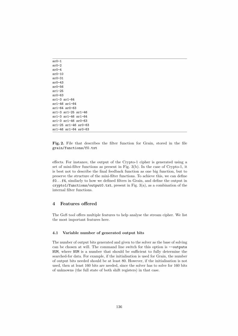
sr0-1

sr0-2

sr0-4

sr0-10

sr0-31

sr0-43

sr0-56

sr1-25

sr0-63

sr1-3 sr1-64

sr1-46 sr1-64

sr1-64 sr0-63

sr1-3 sr1-25 sr1-46

sr1-3 sr1-46 sr1-64

sr1-3 sr1-46 sr0-63

sr1-25 sr1-46 sr0-63

sr1-46 sr1-64 sr0-63

Fig. 2. File that describes the filter function for Grain, stored in the filegrain/functions/f0.txt

effects. For instance, the output of the Crypto-1 cipher is generated using aset of mini-filter functions as present in Fig. 3(b). In the case of Crypto-1, itis best not to describe the final feedback function as one big function, but topreserve the structure of the mini-filter functions. To achieve this, we can definef0. . . f4, similarly to how we defined filters in Grain, and define the output incrypto1/functions/output0.txt, present in Fig. 3(a), as a combination of theinternal filter functions.

4 Features offered

The GoS tool offers multiple features to help analyse the stream cipher. We listthe most important features here.

4.1 Variable number of generated output bits

The number of output bits generated and given to the solver as the base of solvingcan be chosen at will. The command line switch for this option is --outputs

NUM, where NUM is a number that should be sufficient to fully determine thesearched-for data. For example, if the initialisation is used for Grain, the numberof output bits needed should be at least 80. However, if the initialisation is notused, then at least 160 bits are needed, since the solver has to solve for 160 bitsof unknowns (the full state of both shift registers) in that case.

136

f0

f2 f0

f3 f0

f3 f1 f0

f3 f2 f1

f4

f4 f0

f4 f1 f0

f4 f2 f1 f0

f4 f3

f4 f3 f0

f4 f3 f1

f4 f3 f2 f1

(a) The output of Crypto-1, de-scribed as a function of mini-filterfunctions f0. . . f4.

Fin

al

filt

er

12

30

4

(b) The functional diagram of the Crypto-1cipher

Fig. 3. The Crypto-1 cipher (on the right), and the description of its final filterfunction (on the left), made up of multiple micro-functions. The network ofmicro-functions is clearly visible in the functional diagram, and is replicated inGrain-of-Salt with the use of multiple filter functions.

4.2 ANF generation with fact propagation

An Algebraic Normal Form of the described cipher with the given number ofparameters (described below) can be generated. Various statistical data on theANF can also be obtained, such as the size (number of monomials) of the eachfunction, the sum size of all functions, etc.

We call fact propagation the effect of evaluating all equations with respect tothe given information. The given information can be the output of the cipher orother form of helping information. The evaluations might, for instance, cause avariable to be set instantly, for example, if a = bc⊕ d and b = false, d = true

then a = true, and by substituting this fact into other equations, further factscould be found. GoS automatically handles this, and recursively propagates allsuch facts.

Under the aegis of fact propagation GoS also propagates variable equivalences.For example, if a = bc and c = true then a = b, which might lead to further facts.For example, the equation d = b⊕ ab would be changed to d = b⊕ bb = b⊕ b =false allowing the propagation of a further fact. Fact and variable equivalencepropagation considerably shortens problems, which help when they need to besolved using the SAT solver.

4.3 CNF Generation

GoS automatically generates CNF from the fact-propagated ANF using a varietyof mechanisms to optimise the conversion. There are mainly two ways of convertingan equation in ANF to CNF:

137

1. Through cutting long XOR-s, and introducing internal variables for eachmonomial of degree > 1.

2. Through the use of a Karnaugh map generator [15]. Karnaugh maps essentiallydirectly generate the CNF from a truth table, needing no conversion. Thismethod was first used in converting cryptographic ANFs by Soos et al. [3].

Deciding which method to use is non-trivial, and GoS can be given a heuristiccut-off that decides which method to use. The cut-off is given with the command-line parameter --karnaugh NUM where if more than NUM monomials are present inan ANF, the first method is used, while if less or equal, the second method is usedto convert to CNF. Essentially, the first method is relatively straight-forward, butcan generate very non-optimal representation if the number of monomials is small,their average degree is high and they make use of a small number of variables.For example, the Crypto-1 and HiTag2 ciphers’ mini filter functions all fall intothis category, and they are best represented as such. However, if for example thedegree is low, then the Karnaugh map representation is uniquely non-optimal, asKarnaugh maps behave the worst (exponentially) for XOR functions, and theyalso behave very badly with near-XOR functions.

The straight ANF-to-CNF method of simply converting the XOR to CNF andthen introducing internal variables for monomials of degree > 1 is done as follows.Long XOR-s must be cut due to the exponential nature of their conversion: ann-long XOR can only be represented (without introduction of internal variables)as 2n−1 clauses. To overcome this, XOR-s are cut such as:

a⊕ b⊕ c⊕ d⊕ e⊕ f =true↔a⊕ b⊕ c⊕ i =false

d⊕ e⊕ f ⊕ i =true

but the best limit at which XOR-s must be cut, which is usually called the cuttingnumber is not easy to determine. The default is 7 in GoS, but can be changedwith --xorcut NUM. Monomials are expressed in the CNF language through theintroduction of internal variables. For example, the monomial ab is expressed asi2 = ab, leading to the clause-set:

¬i2 ∨ b¬i2 ∨ a

i2 ∨ ¬a ∨ ¬b

An optimisation for the straight ANF-to-CNF conversion is that monomialsin the CNF world can contain negations, i.e. it is no longer necessary to writea ⊕ ab, since that can be simply written as a(1 + b) = a¬b. This optimisation

138

can be applied recursively. For example:

a⊕ b⊕ ab⊕ c⊕ cd =true↔b⊕ a(1⊕ b)⊕ c(1⊕ d) =true↔

1⊕ (1⊕ a)(1⊕ b)⊕ c(1⊕ d) =true↔¬a¬b⊕ c¬d =false

reducing the original 5 monomials into a mere two. Representing these monomialsthat are not free of negations takes exactly the same amount of resources inCNF as representing those that are free of negations, leading to a potentialoverall reduction in the final CNF. The reduction is only potential, as the internalvariables that represent monomials that are used in multiple places need onlybe described once, and the extended monomials could possibly make it moredifficult for the same monomials to appear, limiting their benefits. Therefore, thisoptimisation can be turned off with the command-line switch --noextmonomials.The default is for this optimisation to be turned on, as we have experiencedspeedups using it.

4.4 Dependency tree generation

It is assumed that only the output of the stream cipher is known to the attacker.Therefore, functions that are not connected in some way to the output of thefunction can be discarded: they are internal variables that need not be calculated,since they cannot help solving the internal state. To remove these functions, adependency tree is generated that takes as root all the output bits of the cipher,and generates a tree that reaches the original internal state bits. All functionsthat are not connected to this tree can be discarded.

Dependency tree generation is very important, as it lets the designer describeas many filter functions as he or she wishes: the functions that are not used willnot hamper the solving. For example, some ciphers use filter functions that arespecific to the initialisation phase. Without dependency tree generation, thesefilter functions would be calculated (but not used) during the normal runningphase, slowing down the solver.

4.5 Solving with and without initialisation phase

The GoS tool has two running modes. It can either try to solve for the non-tweakable and non-oned-out parts of the cipher when initialisation is turned on,or it can solve for the entire state when initialisation is turned off. In other words,the two typical scenarios are covered: either the IV is known, the key is unknown,and the initialisation is carried out, or the entire state of the cipher is unknown,but the initialisation is not carried out. This behaviour can be simply switchedusing a command line switch --init yes or --init no.

Typically, with the initialisation turned on, the number of bits to be solved ismuch less. For example, in the case of Grain, the IV is 64, and the one-ed out part

139

is 16 bits, so only 80 bits of the first shift register (i.e. the key) is the unknown.However, the initialisation takes 160 cycles, which greatly increases the difficultyof the resulting set of equations. On the other hand, without initialisation, thenumber of unknown bits increases to 2*80 = 160, but since initialisation is notcarried out, most equations are very short.

4.6 Base shifting

Base shifting can be activated when solving without initialisation. Base shiftingis the name we use for the technique first presented in [3, Sect. 4.3]. There, theauthors show that the base unknown of the cipher can be any moment in time. So,for example, if the number of output bits generated is 200, and no initialisationis used, then the cipher is clocked for 100 bits, with a total length of 100 + 80 =180 (since 80 is the original size of each). Any consecutive 80 bit frame of thiscan be taken as the unknown, as the feedback functions can be re-arranged toclock backwards for these ciphers. This is very advantageous, as typically, thecomplexity increases exponentially starting from a point T , and if we take T tobe near the middle of the time-frame (e.g. at T = 90 in our example), then thetotal complexity of the generated functions are much less than if we had takenthe typical approach, i.e. to take T = 0.

The command line parameter for base shifting is --base-shift NUM whereNUM must be smaller or equal to the number of output bits. For this to work withNUM > 0, the feedback functions of the cipher must be reversible. This is true forCrypto-1, HiTag2, Bivium-B, Trivium, and Grain. Stream ciphers can be createdwhere this is not the case — these stream cipher are, however, usually constrainedin that it is hard to make them work faster through parallel implementation ofthe feedback and filter functions in hardware.

As a concrete example, let us take the Grain cipher, without the initialisationphase switched off. If the number of output bits generated is 200, the base shiftingcan be any number between 0 and 200. For a shifting number x, the unknownsare the states of the shift registers at time x. In other words, if we take each shiftregister as a memory line that does not forget its old contents, then the unknownsare the state variables x . . . x+ 80 of both shift registers. We call these variablesthe reference state variables. When initialisation is turned on, the reference statevariables are simply the variables that are neither tweakable nor one-ed out, i.e.they are the state variables where (typically) the key is loaded.

4.7 Help bit calculation

Help bits are data pieces that are given such that it is easier to solve for the stateof a cipher. These are important, as it is infeasible to wait immense amounts oftime to check whether, for example, the state of Grain can be solved. In orderto circumvent this problem, we give some reference state variables as help bitsto the solver, such that it can solve faster. Once the solving has finished, onecan estimate the time it would take to solve for the whole state of the cipher,without the help bits. The GoS tool offers two types of help bit calculations. One

140

is a probabilistic calculator, and the other is a deterministic calculator, and bothemploy a Monte-Carlo method to achieve their goals. For the following sections,let us assume that V the possible set of variables that can be help bits (i.e. Vcontains exactly the reference state variables).

The Monte-Carlo method, first introduced by Metropolis and Ulam [16] isused in many areas of research such as integration and computer security (e.g. theRabin primality test [17]). It is essentially a randomised algorithm that samples atiny part of the possibly immense space and processes the results to approximatean unknown value for the whole space. In case of the Rabin primality test, theMonte-Carlo algorithm uses a randomised test to decide if a positive integer is aprime or not. The algorithm has a certain chance (< 1/4) to give a false negativeresult, but running the algorithm many times essentially eliminates the chancethat a number is composite.

Deterministic method Since using different reference state variables as helpbits could give different timings, it is non-trivial which ones to use. To achievemaximum performance, we use an approach that we have found to be adequateto find a good set.

We first generate the ANF that describes the cipher given all settings. Then,we set a variable v ∈ V , v ← true, and propagate all changes. We count thenumber of monomials in the resulting ANF. Then, we set v ← false, and againcount the size of the resulting ANF. The sum of these two values is the “score”for this help bit. We perform these steps for each variable in L, and the one thathas the smallest score wins. We now put this winning variable into the orderedset H, and continue the search as follows.

Let us call L the possible set of variables that can be help bits (i.e. L containsexactly the reference state variables). We take a variable v ∈ LH and randomly set all variables in H, plus we set v ← true, and count thescore. We do ten such measures, each time setting the variables in H randomly,and sum the scores. Then, we do the same, but with v ← false, and sum thescores. The sum of these 20 measurements will be the score for this v. We dothis for all v ∈ LH: the variable with the smallest score wins and enters H. At the end of thealgorithm, we reach a point where LH = ∅, and all variables have been ordered in H.

The presented algorithm is a randomised greedy algorithm that tries to finda local minima at each point. Since even a local minima is very difficult to find,the algorithm probabilistically tries to find this local minima, through 20 randomtests. For better local minima finding, the number 20 can be increased to anyeven number, ameliorating the algorithm.

We have found this algorithm to be very powerful in reducing the time tosolve a given cipher. Without such ordering of bits, the speed to solve a certainproblem can be hundreds of times more difficult. The output of this algorithm issimply put a file called “best-bits”, and the variable numbers are simply listed

141

one after the other. If the cryptographer knows a better ordering, this file cansimply be overwritten.

Once the “best bits” file has been generated, it can be used from the programby giving the option --deterBits NUM, where NUM is the number of best bits theprogram should set randomly when generating the problem instances. Averagingthe time it takes to solve these problems and multiplying the average by 2NUM onegets the amount of expected time to solve the cipher.

The program specifically does not include a method to break a cipher, thoughgiven a specific cipher output, it could generate all 2NUM possible problems.Naturally, one of the generated problems would actually break the given outputstream, revealing the key or the state of the cipher (depending on whetherinitialisation was enabled or not).

Probabilistic method The probabilistic method is activated with the commandline switch --probBits NUM and it simply randomly sets a random set of NUM

variables from L and does many runs of these random configurations. The timeit takes to solve these randomly picked instances is then averaged.

To approximate the time it takes to attack the cipher without giving anyvariables we use the following technique. We run many instances of the abovealgorithm with NUM = n, n−1, . . . n−k number of reference state variables, wheren is small enough such that the algorithm is not trivial to solve, and n− k is assmall as possible such that the resulting system is still solved within a reasonableamount of time. The average time is then plotted against the number of referencestate variables given, and the plot is extrapolated to the point where there areno reference state variables given.

Although there is no proof that at any point during NUM = n − k − 1 . . . 0the graph does not suddenly change, we believe this to be extremely unlikely.For the explication of the reasons, let us first define some notions. Let us definetwo problems for a given cipher: problem A is when NUM = x, and problem B iswhere NUM = x− 1, where n ≥ x > 0 but otherwise x is irrelevant. Let us assume,without loss of generality, that V ′ is the set of reference variables selected to beassigned in B. Let the set of reference variables assigned in A be V ′

⋃v. We can

now list the reasons why we believe the graph does not deviate from a straightline if the time is plotted in a logarithmic scale:

– Every problem in B can be directly mapped to 2|V \ V ′| = 2(n − x + 1)problems in A. Since the underlying algorithm of DPLL-based SAT solvers isessentially an intelligent brute-force, we can safely assume it does not behaveworse than a brute-force, and solves the problem B in at most twice the timethan solving any problem in A. This is further underlined by our observationthat SAT solvers branch on the reference state variables — thus the firstbranching of the solver when solving B will indeed be a variable from |V \V ′|

– The more choice of variables a SAT solver has to branch on, the better thedynamic variable branch ordering will work. This means that it is expectedof the solver to solve in less than twice the time problem B with a choice of

142

n− x branch variables, than two problems in A with a choice of n− x− 1branch variables

– Clauses learnt during the solving of A that are independent of the setting ofvariable v cannot be reused between the solving instances. Therefore, it isexpected that problem B can be solved faster than two problems in A, asthe solver in the former case does not need to re-learn these same clauses

– The underlying problem structure does not change between problem A andproblem B

– It is the same underlying randomised solving algorithm that is used to solveboth problem A and problem B

The extrapolation is usually straightforward if a large enough number ofrandomisation steps are involved: the plotted graph is straight if plotted against alogarithmic time. We note that the possibility of extrapolation is an advancementover previous attempts. Previous attempts failed, as they did not introducesufficient randomness into the system. This lack of suitable randomisation meantthat their results were not extrapolateable [18,2].

5 Results

GoS in conjunction with an appropriate SAT solver such as CryptoMiniSat [19]can be used to break Crypto-1 in 40 s, HiTag2 in 214.5 s, and Bivium-B in anapproximated 236.5 s using a a Xeon [email protected] computer. All these figuresare faster than exhaustive search, leading to the breaking of these algorihtms.In the literature we have not found any results that indicated a faster solvingtime for these ciphers using a SAT-based cryptanalsysis, and so we believe thesefigures to be the current state-of-the-art.

6 Conclusions

We have presented Grain of Salt, an integrated package to test stream ciphersagainst SAT solver-based attacks. The tool can flexibly generate with a minimumof user intervention a CNF representation of any shift-register based stream cipher,helping the researcher evaluate the cipher against SAT solver-based algebraicattacks. The input language and the command line options of the tool are easyto use and user-friendly, helping the novice as well as the advanced users toprofit from the tool. We envision that Grain of Salt will be further extended byresearchers to carter for their specific needs, making the tool more diverse andmore useful for the whole of the research community.

Acknowledgements

The author was supported by the RFID-AP ANR Project, project numberANR-07-SESU-009. I would like to thank Karsten Nohl for some initial ideas,notably base-shifting.

143

References

1. Courtois, N.T., Bard, G.V.: Algebraic cryptanalysis of the Data EncryptionStandard. In Galbraith, S.D., ed.: IMA Int. Conf. Volume 4887 of Lecture Notes inComputer Science., Springer (2007) 152–169

2. Eibach, T., Pilz, E., Volkel, G.: Attacking Bivium using SAT solvers. In Buning,H.K., Zhao, X., eds.: SAT. Volume 4996 of LNCS., Springer (2008) 63–76

3. Soos, M., Nohl, K., Castelluccia, C.: Extending SAT solvers to cryptographicproblems. In Kullmann, O., ed.: SAT. Volume 5584 of Lecture Notes in ComputerScience., Springer (2009) 244–257

4. Garcia, F.D., de Koning Gans, G., Muijrers, R., van Rossum, P., Verdult, R.,Schreur, R.W., Jacobs, B.: Dismantling MIFARE Classic. In Jajodia, S., Lopez,J., eds.: ESORICS. Volume 5283 of Lecture Notes in Computer Science., Springer(2008) 97–114

5. Courtois, N., O’Neil, S., Quisquater, J.J.: Practical algebraic attacks on the HiTag2stream cipher. In Samarati, P., Yung, M., Martinelli, F., Ardagna, C.A., eds.: ISC.Volume 5735 of Lecture Notes in Computer Science., Springer (2009) 167–176

6. Canniere, C.D.: Trivium: A stream cipher construction inspired by block cipherdesign principles. In Katsikas, S.K., et al, eds.: ISC. Volume 4176 of LNCS., Springer(2006) 171–186

7. Raddum, H.: Cryptanalytic results on Trivium. Technical Report 2006/039,ECRYPT Stream Cipher Project (2006)

8. Hell, M., Johansson, T., Meier, W.: Grain: a stream cipher for constrained environ-ments. IJWMC 2(1) (2007) 86–93

9. Massacci, F., Marraro, L.: Logical cryptanalysis as a SAT-problem: Encoding andanalysis. Journal of Automated Reasoning 24 (2000) 165–203

10. Courtois, N., Bard, G.V., Wagner, D.: Algebraic and slide attacks on KeeLoq. InNyberg, K., ed.: FSE. Volume 5086 of Lecture Notes in Computer Science., Springer(2008) 97–115

11. The SAGE Group: SAGE mathematics software (2008) http://www.sagemath.org.12. Barrett, E.: Logic2CNF logic solver and converter (March 2010) http://projects.

cs.kent.ac.uk/projects/logic2cnf/.13. Ganesh, V., Dill, D.L.: A decision procedure for bit-vectors and arrays. In Damm,

W., Hermanns, H., eds.: CAV. Volume 4590 of Lecture Notes in Computer Science.,Springer (2007) 519–531

14. Bard, G.V., Courtois, N.T., Jefferson, C.: Efficient methods for conversion andsolution of sparse systems of low-degree multivariate polynomials over GF(2) viaSAT-solvers. Cryptology ePrint Archive, Report 2007/024 (2007)

15. Karnaugh, M.: The map method for synthesis of combinational logic circuits.Transactions of American Institute of Electrical Engineers part I 72(9) (November1953) 593–599

16. Metropolis, N., Ulam, S.: The Monte Carlo method. Journal of the AmericanStatistical Association 44(247) (1949) 335–341

17. Rabin, M.O.: Probabilistic algorithm for testing primality. J. Number Theory 12(1)(1980) 128–138

18. McDonald, C., Charnes, C., Pieprzyk, J.: Attacking Bivium with MiniSat. TechnicalReport 2007/040, ECRYPT Stream Cipher Project (2007)

19. Soos, M.: CryptoMiniSat — a SAT solver for cryptographic problems (2009)http://planete.inrialpes.fr/~soos/CryptoMiniSat2/index.php.

144

Analysis of Trivium by a Simulated Annealing

Variant

Julia Borghoff1, Lars R. Knudsen1, and Krystian Matusiewicz2

1 Department of Mathematics, Technical University of DenmarkJ.Borghoff, [email protected]

2 Institute of Mathematics and Computer Science, Wroclaw University of [email protected]

Abstract. This paper proposes a new method of solving certain classes ofsystems of multivariate equations over the binary field and its cryptanalyticalapplications. We show how heuristic optimization methods such as hill climb-ing algorithms can be relevant to solving systems of multivariate equations.A characteristic of equation systems that may be efficiently solvable by themeans of such algorithms is provided.As an example, we investigate equation systems induced by the problem ofrecovering the internal state of the stream cipher Trivium. We propose animproved variant of the simulated annealing method that seems to be well-suited for this type of system and provide some experimental results.

Keywords. simulated annealing, cryptanalysis, Trivium

1 Introduction

Cryptanalysis focuses on efficient ways of exploiting, perhaps unexpected, structureof cryptographic problems. It could be a difference which propagates with a highprobability through the cipher as used in differential cryptanalysis [6, 2] or a linearapproximation of the non-linear parts of a cipher that holds for many of the possibleinputs as it is the case with linear cryptanalysis [20].

More recently, the so-called algebraic attacks have received much attention. Theyexploit the fact that many cryptographic primitives can be described by sparse mul-tivariate non-linear equations over the binary field in such a way that solving theseequations recovers the secret key or the initial state in the case of stream ciphers.In general, solving random systems of multivariate non-linear Boolean equations isan NP-hard problem [12]. However, when the system has a specific structure, we canhope that more efficient methods may exist.

One technique to tackle such equation systems is linearisation, where each non-linear term is replaced by an independent linear variable. It works only if there areenough linear independent equations in the resulting system. Courtois et al [7] pro-posed the XL algorithm which increases the number of equations by multiplying themwith all monomials of a certain degree. It has been refined to the XSL algorithm [9],which, when applied to the AES, exploits the special structure of the equation system.Neither the XL nor the XSL algorithm have been able to break AES but algebraicattacks were successful in breaking a number of stream cipher designs [8, 1].

In this paper we also investigate systems of sparse multivariate equations. Theimportant additional requirement we make is that each variable appears only in avery limited number of equations. The equation system generated by the key streamgeneration algorithm of the stream cipher Trivium [10] satisfies those properties and

145

will be examined in this paper as our main example. The fully determined Triviumsystems consists of 954 equations in 954 variables. Solving this system allows us torecover the 288-bit initial state.

Our approach considers the problem of finding a solution for the system as anoptimization problem and then applies an improved variant of simulated annealingto it. As opposed to the XL and XSL algorithms, the simulated annealing algorithmdoes not increase the size of the problem, it does not generate more nor change theexisting equations. The only additional requirement is an objective function, calledthe cost function, that should be minimized.

Simulated annealing has been studied in the context of cryptography before. Knud-sen and Meier [19] presented an attack on an identification scheme based on the per-muted perceptron problem (PPP). They found an appropriate cost function whichenabled them to solve the simpler perceptron problem as well as the PPP using asimulated annealing search. The attack showed that the recommended smallest pa-rameters for the identification scheme are not secure. The same identification schemewas later a subject to an improved attack by Clark and Jacob [5]. They used simu-lated annealing to solve a related problem that had solutions highly correlated withthe solution of the actual problem. They also made use of timing analysis where thesearch process is monitored and one can observe that some variables are stuck atcorrect values at an early state and never change again.

With our current experiments, we are not able to break Trivium in the crypto-graphic sense which means with a complexity equivalent to less than 280 key setupsand the true complexity of our method against Trivium is unknown. However, if weconsider the Trivium system purely as a multivariate quadratic Boolean system in 954variables then we are able to solve the system significantly faster than brute force,namely in around 2210 bit flips which is roughly equivalent to 2203 evaluations of thesystem. This shows that our variant of simulated annealing seems to be a promisingtool for solving non-linear Boolean equation systems with certain properties.

2 Hill climbing algorithms

Hill climbing algorithms are a general class of heuristic optimization algorithms thatdeal with the following optimization problem. We have a finite set X of possible con-figurations. Each configuration is assigned a non-negative, real number called cost,or, in other words, we have a cost function defined as f : X → R. For each config-uration x ∈ X a set of neighbours η(x) ⊂ X is defined. The aim of the search is tofind xmin ∈ X minimizing the cost function f(x), f(xmin) = minf(x) : x ∈ X, bymoving from neighbour to neighbour depending on the cost difference between theneighbouring configurations.

Johnson and Jacobsen [15] presented a unified view of many hill climbing algo-rithms by describing conditions on accepting a move from one configuration to an-other. The transition probability pk(x, y) of accepting a move from x to y ∈ η(x) isdefined as the product of a configuration generation probability gi(x, y) and a config-uration acceptance probability Pr[Rk(x, y) ≥ f(y)−f(x)], where Rk(x, y) is a randomvariable and k is an iteration index that is increased by one after a fixed number ofmoves. Algorithm 1 presents a general form of a hill climbing algorithm.

Note that when Rk(x, y) = 0, we obtain a local search algorithm as only movesthat decrease the cost are accepted.

146

Algorithm 1 General formulation of hill climbing algorithmsxbest ← xwhile stopping criterion not met do

k ← 0 set the outer loop counterwhile k < K do

for m = 0, . . . , M − 1 dogenerate a neighbour y ∈ η(x) with probability gk(x, y)compute the cost function f(y) of the candidateif Rk(x, y) ≥ f(y)− f(x) then

x← y accept the moveif f(x) < f(xbest) then

xbest ← x store the best configurationend if

end ifend fork ← k + 1

end whileend while

Simulated annealing Classical simulated annealing algorithm [18] is a special caseof the general hill climbing algorithm presented above with a particular definition ofthe transition probability. The inspiration and the name comes from the process usedin metallurgy to improve the durability of steel and alloys. When a metal is heatedabove its recrystallization temperature, the atoms break from their initial positions inthe crystals and are able to relocate to other places. When slowly cooling down, theatoms are most likely to stay in new positions guaranteeing a lower total energy ofthe system, improving its regular structure and thus also the mechanical properties.

The simulated annealing algorithm uses a key parameter called the temperaturet. The configuration generation probability is taken to be uniform, i.e. each neighbouris equally likely to be picked from each state. The acceptance probability depends onthe difference f(y)−f(x) in cost function between the current state x and the selectedneighbour y and the current temperature tk. The move is always accepted when itdecreases the cost and with probability e−(f(y)−f(x))/tk when the cost increases. Interms of the general formulation presented above, we get this behaviour when wedefine Rk(x, y) = −tk ln(U), where U is a uniform random variable on [0, 1].

Note that when the temperature tk is high, many cost-increasing moves are ac-cepted. When the temperature is lower, worsening moves are less and less likely to beaccepted.

The way the “temperature” tk of the system decreases over time (k) is called thecooling schedule. The condition necessary for the global convergence of the methodis that tk ≥ 0 and limk→∞ tk = 0. In practice, two most commonly used coolingschedules are the exponential cooling schedule tk = α · βk for some parameter 0 <β < 1 and the logarithmic cooling schedule tk = α/ log2(k+1) proposed in [13], whereα is a constant corresponding to the starting temperature.

3 Trivium system as an optimization problem

Trivium [10] is an extremely simple and elegant stream cipher that was submitted tothe ECRYPT eStream project. It successfully withstood significant cryptanalyticalattention [21–23, 3] and became part of the portfolio of the eStream finalists.

147

To our knowledge, there is no attack on Trivium faster than the exhaustive keysearch so far. However, several attacks have been proposed which are faster than thenaive guess-and-determine attack with complexity 2195 which was considered by thedesigners [10]. A more intelligent guess-and-determine attack with complexity 2135

using a reformulation of Trivium has been sketched in [17]. Furthermore, Maximovand Biryukov [21] described an attack with complexity 285.5 and Raddum proposed anew algorithm for solving non-linear Boolean equations and applied it to Trivium in[22]. The attack complexity was 2164. There have been further attacks on the smallscale variant called Bivium as well as fault attacks on Trivium but we do not go intothe details here.

Trivium has an 80-bit key, an 80-bit IV and 288 bits of the internal state (s1, . . . , s288).At each clock cycle it updates only three bits of the state and produces one bit of thekey stream using the following procedure.

for i = 1, 2, . . . dozi ← s66 + s93 + s162 + s177 + s243 + s288 Generate output bit zi

ti,1 ← s66 + s93 + s91 · s92 + s171

ti,2 ← s162 + s177 + s175 · s176 + s264

ti,3 ← s243 + s288 + s286 · s287 + s69

(s1, s2, . . . , s93)← (ti,3, s1, . . . , s92)(s94, s95, . . . , s177)← (ti,1, s94, . . . , s176)(s178, s179, . . . , s288)← (ti,2, s178, . . . , s287)

end for

During the key setup phase, the key is loaded into the first 80 bits of the state,followed by 13 zero bits, then the IV is loaded into the next 80 bits of the state andthe remaining bits are filled with constant values. Then 4 ·288 clockings are computedwithout producing any keystream bits. Our results do not depend on this procedure.

The initial state which is the state of the registers at the time when the keygeneration starts can be expressed as system of sparse linear and quadratic Booleanequations [22]. We consider the initial state bits as variables and label them withs1 . . . , s288. In each clocking of the Trivium algorithm three state bits are updated.The update function is a quadratic Boolean function of the state bits. In order to keepthe degree low and the equations sparse we introduce new variables for each updatedstate bit ti,1, ti,2, ti,3. We get the following equations from the first clocking

s66 ⊕ s93 ⊕ s91 · s92 ⊕ s171 = s289

s162 ⊕ s177 ⊕ s175 · s176 ⊕ s264 = s290

s243 ⊕ s288 ⊕ s286 · s287 ⊕ s69 = s291

s66 ⊕ s93 ⊕ s162 ⊕ s177 ⊕ s243 ⊕ s288 = z

(1)

where the last equation is the key stream equation with z being the known key streambit.

After observing 288 key stream bits we can set up a fully determined system of954 Boolean equations in 954 unknowns [22]. We only need to consider 954 equationsand unknowns instead of 1152 since we do not care about the last 66 state updatesfor each register. These variables will not be used in the key stream equation becausethe new bits are not used for the key stream generation before 66 further clockingsof the cipher. By clocking the algorithm more than 288 times we can easily obtain anoverdetermined system. We know that the initial state together with the correspond-ing updated state bits fulfills all the generated equations (1). On the other hand,for a random point each equation is satisfied with probability 1

2 . If we consider the

148

problem of solving the Trivium equation system as an optimization problem which issuitable for hill climbing algorithms (cf. Section 2) X = 0, 1954 is the set of possibleconfigurations. As a cost function f : X → R we count the number of not satisfiedequations in the system. We know that the minimum of the cost function is 0 and thatthe initial state of the Trivium system is a configuration for which the cost functionis minimal. Of course there might be other optimal solutions. However, it is easy tocheck if the solution we found is the desired one. That a configuration is an optimalsolution for the discrete optimization problem means that it generates the same first288 bits of keystream than the initial state we are looking for. But it is unlikely thatthe keystream will be the same for the following keystream bits. Therefore we cancheck if a solution is the desired one by observing a few more keystream bit andcomparing them to the keystream generated by the solution. In our experiments it isunlikely that multiple solutionss occur because we set some of the variables to therecorrect values and consider therefore a highly overdetermined equation system.

4 Properties of Trivium landscapes

Hill climbing algorithms are sensitive to the way in which the cost function changeswhen moving between configurations. Best results are obtained when a move from aconfiguration x ∈ X to one of the neighbours η(x) does not change the value of thecost function too much.

In our case we move from one configuration to another by flipping the value of asingle variable. But each variable appears in at most 8 equations and in 6 equations onaverage, so when moving to a neighbour of the current configuration the cost functionwill change by at most 8. Furthermore, changing the value of a single variable willchange the value of the equation with probability 1 if the variable appears in a linearterm and with probability 1

2 if the variable appears in a quadratic term. In the lattercase flipping the value of a variable will just change the outcome of the equation ifthe other variable in the quadratic term is assigned to ’1’. If a variable appears in themaximum of eight equations it appears in two equations in the quadratic term only.(Here it is important to note that each variable appears only once in an equation.)The expected number of equations which change their outcome is 7. Additionally itis unlikely that flipping the value of a variable changes the outcome of all equationswhich contain this variable in the same direction or respectively it is unlikely thatall equations which contain the variable have the same outcome for the configurationbefore the flip. (Of course the case that a lot or even all equations have the sameoutcome will appear with higher probability the closer we are to the minimum.)

From these observations we infer that even if we move from a configuration x toone of its neighbours by flipping the value of a variable which appears in 8 equationswe do not expect that the value of the cost function changes by 8 in almost all of thecases.

We confirmed this by the following experiment. We generated a Trivium systemfor a random key and calculated the cost function for a random starting point. Thenwe chose a neighbour configuration of our starting point and recorded the absolutevalue of the change in the cost function. To simulate being close to the minimum weset a number of bits to the correct solution but we allowed those bits to be flipped tomove to a neighbouring configuration. The results are summarized in Table 1.

These properties of Trivium cost landscapes can be captured more formally usingthe notion of NK-landscapes and landscape auto-correlation as follows.

149

Table 1. Change of the cost function when moving to a neighbour configuration:The first row denotes the number of preassigned bits we use to simulate different distancesfrom the minimum. We count how often out of 10000 trials the cost function changes by 0to 8 units. The last row gives us the average change of the cost function.

i 0 100 200 300 400 500 600 700 800 900 954

0 1714 1702 1685 1560 1309 1052 944 767 601 264 01 3253 3246 3297 3158 2641 2143 1856 1550 1120 389 342 2248 2235 2240 2241 1930 1720 1385 1172 937 1001 10623 1557 1571 1550 1659 1821 1757 1488 1278 1258 1515 15374 675 665 668 754 1024 1020 911 810 741 596 6485 386 400 380 409 691 940 1088 1078 1024 1068 11606 127 128 130 164 409 916 1372 1630 1866 2002 20497 32 44 41 46 165 439 837 1352 1854 2297 25348 8 9 9 9 10 13 119 363 599 868 976

average change 1.81 1.824 1.814 1.9 2.32 2.83 3.32 3.85 4.38 4.97 5.3

4.1 Trivium systems and NK-landscapes

NK-landscapes were introduced by Kaufmann [16] to model fitness landscapes withtunable “ruggedness”. An NK-landscape is a set of configurations X = 0, 1n to-gether with the cost function defined as

f(x) =n∑

i=1

fi(xi; xπi,1 , . . . , xπi,k) ,

where each πi is a tuple of k distinct elements from the set 1, . . . , n \ i. In otherwords, the cost function of an NK-landscape is a sum of n local cost functions fi, eachone of them depending on the main variable xi and a set of k other variables. In arandom neighbourhood model, the k indices are selected randomly and uniformly foreach fi. Depending on the value of k, we get either smooth landscapes with relativelyfew local minima when k is small and rugged landscapes for large values of k.

The Trivium optimization problem can be seen as such combinatorial landscape.Consider the basic system of equations. We define each fi as the contribution of i-thequation (either 0 or 1 depending on whether it is satisfied). Each equation dependson six distinct variables, we verified by a computer program that indeed we can alwayspick one of them as the main variable leaving exactly five other ones for each equation.Trivium optimization problem can thus be seen as an instance of NK-landscape withn = 954 and k = 5, a rather small value hinting at a certain smoothness of thislandscape.

4.2 Landscape auto-correlation

Another measure of landscape ruggedness is the notion of landscape correlation in-troduced by Weinberger [24]. We will follow the exposition by Hordijk [14]. The mainidea is to perform a random walk on the landscape via neighbouring points. At eachstep, the cost function yt is recorded. That way a sequence (yt)t=1...T is obtained andwe compute its auto-correlation coefficients.

The auto-correlation of a sequence (yt) for the time lag i is defined as

ρi = Corr(yt, yt+i) =E[yt · yt+i]− E[yt]E[yt+i]

V ar[yt]

150

where E means the expected value and V ar variance of a random variable. Estimatesri of these auto-correlations ρi are

ri =

∑T−it=1 (yt − y)(yt+i − y)

∑Tt=1(yt − y)2

where y means the mean value of yt. Here a large auto-correlation coefficient corre-sponds to a smooth landscape. An important assumption that has to be made forsuch analysis to be meaningful is that the landscape is statistically isotropic. Thismeans that the statistics of the time series generated by a random walk are the same,regardless of the starting point. Only then a random walk is “representative” of theentire landscape. By computing correlation coefficients for many random walks start-ing at different points we experimentally verified that the Trivium landscape can beseen as isotropic.

Selected correlation coefficients computed for a basic version of Trivium systemand overdefined versions are presented in Table 2. Clearly, generating the overdefinedsystem makes the landscape smoother.

Table 2. Correlation coefficients for landscapes generated by Trivium systems of differentsizes. n denotes the number of variables in the system.

keystream length n r(1) r(10) r(20) r(30) r(40) r(50)

288 954 0.989 0.896 0.803 0.720 0.646 0.580576 1818 0.9941152 3546 0.997

5 Solving Trivium system with modified simulated annealing

The properties of landscapes generated by the Trivium system of equations suggestthat it might be possible to employ stochastic search methods such as simulatedannealing to try to find a global optimum and thus recover the secret state of thecipher. In this section we report the results of our experiments in this direction.

Initial experiments with standard simulated annealing were not very encouraging.To be able to solve the Trivium system in reasonable time, we needed to simplifythe initial system by setting around 600 out of 954 variables to their correct valuesthroughout the search.

We experimented with the algorithm and its various modifications and found onethat yielded a significant improvements over the standard algorithm. The algorithmworks as follows. As with standard simulated annealing, we randomly generate aneighbour. If the cost decreases, we accept this move. If not, instead of acceptingwith probability related to the current temperature, we pick another neighbour andtest that one. If after testing a certain number of neighbours we cannot find anycost decreasing move, we accept the increasing move with some probability, just asin the plain simulated annealing. The parameter of this procedure is the number ofadditional candidates to test before accepting cost increase.

If the parameter is zero, we get plain simulated annealing. On the other end of thespectrum, if we test all possible neighbours, it is easy to see that we get an algorithmthat is equivalent to local search, we look for any possible decreasing move and wefollow it. When we are in a local minimum, we enter a loop, we finally accept one

151

of the cost increasing candidates but in the next move we always go back to thelocal optimum we found. Setting the parameter between those extremes yields anintermediate algorithm.

In practice, we used a probabilistic variant of this approach that randomly selectsneighbours until it finds one with smaller cost or it exceeds the number of tests definedas a parameter nochangebound. This algorithm is presented in Alg. 2.

Algorithm 2 Modified version of simulated annealingxbest ← xT ← α initial temperature parameter is αk ← 0 set the outer loop counterwhile T > 1 do

for m = 0, . . . , M − 1 do parameter M is the number of inner runsgenerate a neighbour y ∈ η(x) uniformlyif f(y) < f(x) then if cost decreased

x← y accept the moveif f(x) < f(xbest) then found a new best value

xbest ← x store the best configurationnc← 0 reset the neighbor counterif f(xbest) = 0 then if we found a solution

return xbest finish and return itend if

end ifelse the candidate cost is higher

nc← nc + 1if (nc > nochangebound) ∧ (exp((f(y)− f(x))/T > rnd[0, 1]) then

x← y accept the movenc← 0 reset the counter of tested neighbours

end ifend if

end fork ← k + 1T = α/ log2(k ·M) Logarithmic cooling schedule

end while

The relationship between the number of neighbours tested and the time it tookto find a solution (measured in the number of neighbours tested) is presented inFig 1. Values of nochangebound below 25 result in running times exceeding 240 flips.It suggests that the proper choice of nochangebound is critical for the efficiency of thesimulated annealing, in particular, it cannot be too small.

6 Experimental results

In this section we report results of our computational experiments with the basicequation system generated by the problem of recovering internal state of Trivium.We took the fully determined system with 954 equations and variables obtained afterobserving 288 bits of the keystream.

We made some comparisons between exponential and logarithmic cooling schedulesand from our limited experience the logarithmic cooling schedule performed better inmore cases, so we decided to pick that one for our further tests.

152

25

26

27

28

29

30

31

32

0 50 100 150 200 250 300 350 400

nochangebound

α = 31

α = 33+

+

+

+

+

+

+

+

+

+

+

+

α = 35

32

33

34

35

36

37

38

39

40

50 100 150 200 250 300 350 400

nochangebound

α = 31

α = 33

+

+

+

+

+

+

+

++

+

+

α = 35

Fig. 1. Influence of nochangebound parameter on the efficiency of simulated annealing ap-plied to basic Trivium system for three values of initial temperature α. Other parametersare M = 1024 (cf. Alg. 2), averages are over 10 tests. In the top figure we guessed 200 firstbits of the state, in the bottom one 180 bits.

The values of α were picked based on empirical observations. Too large α resultedin prolonged periods of almost-random walks where there was no clear sign that anyoptimization might occur. Too small values gave the behavior similar to a simple localsearch when the process was getting stuck in some shallow local optima. After a fewtrials we decided to use the initial temperature parameter α = 35.

For each number of bits of the state fixed to their correct values (preassigned) weran ten identical tests with different random seeds testing various values of nochange-bound parameter (from the set 100, 150, 175, 200, 250, 300). After the test batchfinished, we picked that value of nochangebound that yielded lowest search time. Wemanaged to obtain optimal values for nochangebound for 200, 195, 190, 185, 180, 175and 170 preassigned bits where we set the values of the first bits of the internal state.We use this optimal nochangebound to estimate the total complexity of the attack.The graph is presented in Fig. 2. The total complexity is the product of the num-

153

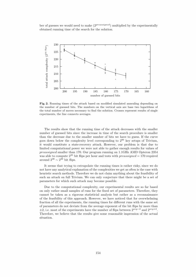
ber of guesses we would need to make (2preassigned) multiplied by the experimentallyobtained running time of the search for the solution.

200

205

210

215

220

225

230

160165170175180185190195200

tota

latt

ack

com

ple

xity

(2bit

flip

s)

number of guessed bits

+

+

+

+

+

++

+

+

++

++

+

+

++

+ +

++

+

+

++

+

++

++

+

+

+ +

+

+

+

+ +

+

+

+

+

+

+

+

+

+ +

++

+

++

++

+

++

++

++

+

++

++

++

+

+

+

+

+

+

+

Fig. 2. Running times of the attack based on modified simulated annealing depending onthe number of guessed bits. The numbers on the vertical axis are base two logarithms ofthe total number of moves necessary to find the solution. Crosses represent results of singleexperiments, the line connects averages.

The results show that the running time of the attack decreases with the smallernumber of guessed bits since the increase in time of the search procedure is smallerthan the decrease due to the smaller number of bits we have to guess. If the curvegoes down below the complexity level corresponding to 280 key setups of Trivium,it would constitute a state-recovery attack. However, our problem is that due tolimited computational power we were not able to gather enough results for values ofpreassigned smaller than 170. Our program running on 1.1GHz AMD Opteron 2354was able to compute 235 bit flips per hour and tests with preassigned = 170 requiredaround 238 ∼ 239 bit flips.

It seems that trying to extrapolate the running times is rather risky, since we donot have any analytical explanation of the complexities we get as often is the case withheuristic search methods. Therefore we do not claim anything about the feasibility ofsuch an attack on full Trivium. We can only conjecture that there might be a set ofparameters for which such attack may become possible.

Due to the computational complexity, our experimental results are so far basedon only rather small samples of runs for the fixed set of parameters. Therefore, theycannot be taken as a rigorous statisticial analysis but rather as a reconnaissanceof the feasibility of this approach. However, we have noticed that for overwhelmingfraction of all the experiments, the running times for different runs with the same setof parameters do not deviate from the average exponent of the bit flips by more than±2, i.e. most of the experiments have the number of flips between 2avg−2 and 2avg+2.Therefore, we believe that the results give some reasonable impression of the actualsituation.

154

7 Some variations

The previous section presented the set of our basic experiments. However, there isa multitude of possible variations of the basic setup which could possibly lead tobetter results. In this section we mention some variations of the search problem weconsidered while looking for possible optimizations.

7.1 Guessing strategy

In order to lower the complexity of solving the equation system we set some of thevariables to their correct values. However, the search complexity depends on whichvariables we choose.

We used different guessing strategies for pre-assigning variables and compared theinfluence on the running time of our algorithm. We used the following strategies toguess subsets of the state bits:

1. Select the first variables of the initial state.2. Select the first variables of each register of the initial state.3. Select the last variables of the initial state.4. Select the last variables of the each register of the initial state.5. Select the most frequent variables. These are the variables which are introduced

by the update function at the beginning of the key stream generation. We guessvalues for variable s289 and the consecutive ones in this case.

6. An adaptive pre-assignment strategy which is similar to the ThreeFour strategyin [11] (see Subsection 7.1).

7. Select the variables in such a way that the equation interdependence measure isminimal. (see Subsection 7.1).

It turns out that the best guessing strategy of the ones we tested is to guess the firstbits of the initial state. In addition to a pre-assignment of variables we can determinethe value of further variables by considering the linear and quadratic equations (seebelow). We use this technique in the adaptive pre-assignment strategy.

Table 3. Running time for different pre-assignment strategies. nochangebound=110, 190 bitsare preassigned, average taken over ten runs.

first bits of theinitial state

most frequentbits

first bit ofevery register

last bit of theinitial state

last bit ofeach register

average 29.5 33.0 34.5 31.2 36.4

Adaptive pre-assignment strategy In this pre-assignment strategy we use thefact that assigning 5 of the variables in a linear equation will uniquely determine the6th variable. Starting with an arbitrary linear equation we guess and pre-assign 5 ofthe 6 variables, determine the value of the remaining variable and assign this to itsvalue. We know that a large fraction of the variables appear in two linear equations.So in the next round of pre-assignment we pick an equation in which at least onevariable is already assigned. That means we only have to guess at most 4 variable toget one for free. We continue until we have made the maximum number of guesses orwe cannot find an equation in which one variable is already assigned. In the latter case

155

we just have to pick an equation without preassigned variables and run the algorithmagain until we made the maximum number of guesses.

Additionally we also use the quadratic equations to determine the value of vari-ables.

The advantage of this pre-assignment strategy is that we can assign many morevariables than we actually have to guess. Table 4 gives us an impression of this ad-vantage.

Table 4. The table shows how many bits additional to the guessed bits can be assignedusing the adaptive pre-assignment strategy.

# guessed bits # assigned bits additional assigned bits in %

5 6 20%50 66 32%

100 135 35%200 281 40.5%

The disadvantage is that we instead of making the equations sparser we fix someequations to be zero. That means that there are less equations left which contain freevariables but the maximum number of equations in which a variables appears is still8. Therefore a variable influences a higher percentage of equations.

Minimizing equation interdependency If all the equations used different sets ofvariables, it would be trivial to solve the system by a simple local search. However,variables appear in many equations and changing the value of one of them influencesother equations at the same time. This suggests the idea of guessing (pre-assigning)bits to minimize the number of variables shared by many equations and thus reducethe degree of mutual relationships between equations.

Capturing this intuition more formally, let Ei be an equation and let V(Ei) denotethe set of not preassigned variables that appear in the equation. We can define themeasure of interdependence of two equations Ei, Ej as

IntrDep(Ei, Ej) = |V(Ei) ∩ V(Ej)| .

If the measure is zero, equations use different variables and we can call them separated.Note that pre-assigning any bit that is used by both equations decreases the value ofinterdependence.

To capture the notion of equations interdependence in the whole system of Triviumequations E, the following measure could be used

∑

e,g∈E,e=g

|V(e) ∩ V(g)|2 . (2)

We used the sum of squares to prefer systems with more equations with only fewactive (non-preassigned) variables over less equations that have more active variables,but it is possible to use an alternative measure without the squares,

∑

e,g∈E,e=g

|V(e) ∩ V(g)| . (3)

The algorithm for pre-assigning bits to minimize the above measure is rathersimple. We start with computing the initial interdependence of the system. Then, we

156

temporarily pick a free variable and assign it to compute the new interdependence ofthe system. If this value is smaller than the current record, we remember it as a newrecord. After we test all possible candidates, we pick the record one and assign it forgood. We repeat this procedure until we get the required number of preassigned bits.

We performed an experiment that compared the results of the reference pre-assignment strategy fixing the first 190 bits of the state with two variants minimizing(2) and (3). Results presented in Table 5 are interesting. It seems that in spite ofsignificant smoothening of the landscape indicated by higher values of the coefficientξ the first strategy minimizing (2) significantly worsens the running time. A pos-sible explanation may be that the landscape became more like “golf-course” withlarge areas without any direction and only very small attraction basins leading toglobal solution(s). Another possibility is that for such systems, different parameterof nochangebound is preferred. The second variant minimizing (3) seems to be onlyslightly better than setting the first bits, but more tests would be needed for moreparameters to decide any definite advantage.

Table 5. Running times and landscape auto-correlation coefficients ξ for bit pre-assignmentstrategies minimizing equation interdependence. Experiments used α = 33, M = 1024,nochangebound = 110.

strategy: reference Case 1 Case 2

avg: 29.34 38.9 28.72

ξ 90.1 97.4 96.1

7.2 Using overdefined systems

Results on landscape auto-correlation suggest that using overdefined systems mayyield landscape with better structural properties. However, this happens at the ex-pense of a larger set of variables and equations we have to deal with. Our experimentalresults on overdefined systems suggest that the gain we get from a better landscapeis offset by the larger system size so search times are actually not better.

7.3 Variable persistence

According to [4, 5] while using simulated annealing to some optimization problems,one can observe a bias in the frequency of assigning values to variables during thesimulated annealing procedure. This bias is related to the solution of the system andobserving it can give some information on the solution we are looking for.

We made some experiments that investigated if configurations of local minima(states we run into after a long cooling run) have variables correlated with the globalminimum state. In our limited experiments with the basic Trivium system we did notobserve any such correlations.

8 Conclusions and future directions

We presented a new way of approaching the problem of solving systems of sparse,multivariate equations over the binary field. We represent them as combinatorial op-timization problems with the cost function being the number of not satisfied equations

157

and then we apply some heuristic search methods, such as simulated annealing to solvethem.

We showed that such systems may be relevant in cryptography by giving an ex-ample of the system generated by the problem of recovering the internal state of thestream cipher Trivium.

Our experimental results were focused on Trivium system and they seem to bepromising but for now they do not seem to pose any real threat to the security of thisalgorithm.

We hope that this paper will serve as a starting point for further research in thisdirection. There are many open problems in this area, the most obvious ones are theselection of better parameters of the search procedures and analytically estimatingthe possible complexity of such algorithms.

The other interesting direction seems to be the investigation of alternative costfunctions. In all our experiments we use the simplest measure counting the number ofnot satisfied equations. However, many results in heuristic search literature suggestthat the selection of a suitable cost function may dramatically change the efficiencyof a search. The question of determining whether in our case there exist measuresbetter than the one we used is still open.

References

1. F. Armknecht and M. Krause. Algebraic attacks on combiners with memory. In Advancesin Cryptology – CRYPTO 2003, volume 2729 of LNCS, pages 162–175. Springer, 2003.

2. E. Biham and A. Shamir. Differential Cryptanalysis of the Data Encryption Standard.Springer-Verlag, 1993.

3. J. Borghoff, L. R. Knudsen, and M. Stolpe. Bivium as a mixed-integer linear program-ming problem. In Cryptography and Coding, 12th IMA International Conference, volume5921 of LNCS, pages 133–152. Springer, 2009.

4. P. Chardaire, J. L. Lutton, and A. Sutter. Thermostatistical persistency: A powerfulimproving concept for simulated annealing algorithms. European Journal of OperationalResearch, 86(3):565–579, Nov. 1995.

5. J. A. Clark and J. L. Jacob. Fault injection and a timing channel on an analysis tech-nique. In Advances in Cryptology – EUROCRYPT 2002, volume 2332, pages 181–196.Springer, 2002.

6. D. Coppersmith. The data encryption standard (DES) and its strength against attacks.IBM Journal of Research and Development, 38(3):243–250, 1994.

7. N. Courtois, E. Klimov, J. Patarin, and A. Shamir. Efficient algorithms for solvingoverdefined systems of multivariate polynomial equations. In B. Preenel, editor, Advancesin Cryptology – EUROCRYPT 2000, volume 1807 of LNCS, pages 392–407. Springer-Verlag, 2000.

8. N. Courtois and W. Meier. Algebraic attacks on stream ciphers with linear feedback. InAdvances in Cryptology – EUROCRYPT 2003, volume 2656 of LNCS, pages 644–644.Springer, 2003.

9. N. T. Courtois and J. Pieprzyk. Cryptanalysis of block ciphers with overdefined systemsof equations. In Advances in Cryptology – ASIACRYPT 2002, volume 2501 of LectureNotes of Computer Science, pages 267–287. Springer-Verlag, 2002.

10. C. De Canniere and B. Preneel. Trivium – a stream cipher construction inspired byblock cipher design principles. eSTREAM, ECRYPT Stream Cipher Project, Report2005/030 (2005-04-29), 2005. http://www.ecrypt.eu.org/stream/papers.html.

11. T. Eibach, E. Pilz, and S. Steck. Comparing and optismising two generic attacks onBivium. In SASC, 2008.

12. A. S. Fraenkel and Y. Yesha. Complexity of solving algebraic equations. Inf. Process.Lett., 10(4/5):178–179, 1980.

158

13. S. Geman and D. Geman. Stochastic relaxation, Gibbs distributions, and the bayesianrestoration of images. IEEE Transactions on Pattern Analysis and Machine Intelligence,6(6):721–741, 1984.

14. W. Hordijk. A measure of landscapes. Evolutionary Computation, 4(4):335–360, 1996.15. A. W. Johnson and S. H. Jacobson. A class of convergent generalized hill climbing

algorithms. Applied Mathematics and Computation, 125(2-3):359–373, 2002.16. S. A. Kauffmann. The Origins of Order: Self-Organization and Selection in Evolution.

Oxford University Press, 1993.17. S. Khazaei. Re: A reformuation of TRIVIUM. Posted on the eSTREAM Forum, 2006.18. S. Kirkpatrick, J. Gelatt, C. D., and M. P. Vecchi. Optimization by Simulated Annealing.

Science, 220(4598):671–680, 1983.19. L. R. Knudsen and W. Meier. Cryptanalysis of an identification scheme based on the

permuted perceptron problem. In Advances in Cryptology – EUROCRYPT’99, volume1592, pages 363–374. Springer, 1999.

20. M. Matsui. Linear cryptoanalysis method for DES cipher. In Advances in Cryptology –EUROCRYPT’93, volume 765 of LNCS, pages 386–397. Springer, 1993.

21. A. Maximov and A. Biryukov. Two trivial attacks on Trivium. In Selected Areas inCryptography – SAC 2007, volume 4876 of LNCS, pages 36–55. Springer, 2007.

22. H. Raddum. Cryptanalytic results on Trivium. eStream, 03 2006. available fromhttp://www.ecrypt.eu.org/stream/papersdir/2006/039.ps.

23. M. S. Turan and O. Kara. Linear approximations for 2-round trivium. In Security ofInformation and Networks – SIN 2007, pages 96–105. Trafford Publishing, 2007.

24. E. Weinberger. Correlated and uncorrelated fitness landscapes and how to tell thedifference. Biological Cybernetics, 63(5):325–336, Sept. 1990.

159

proceedings of the ecrypt workshop on tools for cryptanalysis 2010

Documents