proceedings of the 19th european young statisticians meeting
TRANSCRIPT

Proceedings of the
19th European Young
Statisticians Meeting
August 31 – September 4, 2015
Prague
Stanislav Nagy
(editor)

Proceedings of the 19th European Young Statisticians Meeting.Prague, August 31 – September 4, 2015Stanislav Nagy, editorPrague 2015.
ISBN 978-80-7378-301-3
Editor:Stanislav Nagy, [email protected]
Department of Probability and Mathematical StatisticsFaculty of Mathematics and PhysicsCharles University in PragueSokolovska 83, 186 75 Praha 8 – Karlın, Czech Republic.
Published by MATFYZPRESSPublishing House of the Faculty of Mathematics and PhysicsCharles University in PragueSokolovska 83, 186 75 Praha 8, Czech Republicas the 495. publication.The publication didn’t pass the review or lecturer control.Prague 2015

Scientific Programme Committee
Charles University in Prague, Czech Republic
• Marie Huskova
• Matus Maciak
• Stanislav Nagy
Local Organizing Committee
Charles University in Prague, Czech Republic
• Zdenek Hlavka
• Daniel Hlubinka
• Marie Huskova
• Matus Maciak
• Marek Omelka
• Marie Turcicova
Conference Partners


Preface
The first European Young Statisticians Meeting was organized in 1978 (Wilt-shire, Great Britain), the second one in 1981 (Bressanone, Italy), and since thenregularly every two years in different European countries.
From the very beginning the idea of the event is that young researchers from dif-ferent countries come together and establish new research contacts at the beginningof their scientific careers.
In line with previous meetings, each of the representatives from selected Euro-pean countries suggested at most two young researchers to participate in the Meet-ing. Also, five distinguished researchers have been invited to give plenary lectures.
We hope that you find the Meeting interesting and useful.
Welcome to the 19th EYSM 2015 in Prague. Enjoy the city, its history, itsarchitecture and culture, and have a great time!
Local Organizing CommitteePrague, July 2015

ContentsMohamed Amghar and Maarten Jansen:
Optimal Bandwidths for Multiscale Local Polyno-mial Decompositions . . . . . . . . . . . . . . . . . . . . . . 1
Slav Angelov:Modelling Company Performance Based on Finan-cial Ratios . . . . . . . . . . . . . . . . . . . . . . . . . . . . 7
Oykum Esra Askin and Deniz Inan:Weibull-Poisson Regression Model with Shared Ga-mma Frailty . . . . . . . . . . . . . . . . . . . . . . . . . . . 8
Irina Adriana Bancescu:A Mentenance Model with a Quasi Generalized Lind-ley Distribution . . . . . . . . . . . . . . . . . . . . . . . . . 9
Bogdan Corneliu Biolan:The Weighted Log-Lindley Distribution and Its Ap-plications to Lifetime Data Modeling . . . . . . . . . . . 10
Melanie Blazere, Fabrice Gamboa and Jean-Michel Loubes:Partial Least Squares - A New Statistical Insightthrough Orthogonal Polynomials . . . . . . . . . . . . . . 12
Damian Brzyski:The Selection of Relevant Groups of ExplanatoryVariables in GWA Studies . . . . . . . . . . . . . . . . . . 18
Katarına Burclova and Andrej Pazman:Experience with Linear Programming for Experi-mental Design . . . . . . . . . . . . . . . . . . . . . . . . . . 22
Massimo Cannas and Bruno Arpino:Propensity Score Matching with Clustered Data . . . . 24
Ivor Cribben and Yi Yu:Estimating Whole Brain Dynamics Using SpectralClustering . . . . . . . . . . . . . . . . . . . . . . . . . . . . 30
Antonio Cuevas, Pamela Llop and Beatriz Pateiro-Lopez:On the Estimation of the Central Core of a Set.Algorithms to Estimate the λ-Medial Axis . . . . . . . . 31
vi
Jirı Dvorak:Model Fitting for Space-Time Point Patterns UsingProjection Processes . . . . . . . . . . . . . . . . . . . . . . 34
Mark Fiecas and Hernando Ombao:The Evolving Evolutionary Spectrum . . . . . . . . . . . 40
Iurii Ganychenko and Alexei Kulik:Weak Rates of Approximation of Integral-Type Func-tionals of Markov Processes . . . . . . . . . . . . . . . . . 45
Antoine Godichon:Recursive Estimation of the Median Covariation Ma-trix in Hilbert Spaces . . . . . . . . . . . . . . . . . . . . . 50
Thomas Gueuning and Gerda Claeskens:Statistical Inference for the Sparse Parameter of aPartially Linear Single-Index Model . . . . . . . . . . . . 56
Johannes Heiny and Thomas Mikosch:Random Matrix Models with Heavy Tails . . . . . . . . 62
Jozef Jakubık:Comparison of Methods for Variable Selection inHigh-Dimensional Linear Mixed Models . . . . . . . . . 64
Jana Jankova and Sara van de Geer:Confidence Regions for High-Dimensional Sparse Mod-els . . . . . . . . . . . . . . . . . . . . . . . . . . . . . . . . . 69
Tobias Kley:Asymptotic Theory for Copula Rank-Based Perio-dograms . . . . . . . . . . . . . . . . . . . . . . . . . . . . . . 70
Dessislava Koleva and Mariyan Milev:Application of Dividend Policies to Finite DifferenceMethods in Option Pricing . . . . . . . . . . . . . . . . . . 76
Kristof Kormendi and Gyula Pap:Estimation of the Offspring Mean Matrix in 2-TypeCritical Galton-Watson Processes . . . . . . . . . . . . . 81
Jurgita Markeviciute:Invariance Principle Under Self-Normalization forAR(1) Process . . . . . . . . . . . . . . . . . . . . . . . . . . 82
vii

Jari Miettinen, Klaus Nordhausen, Hannu Oja and Sara Task-inen:ICA Based on Fourth Moments . . . . . . . . . . . . . . . 88
Frederik Riis Mikkelsen:Computational Aspects of Parameter Estimation inOrdinary Differential Equation Systems . . . . . . . . . . 94
Yuriy Mlavets and Yuriy Kozachenko:On Calculation of the Integrals Depending on a Pa-rameter by Monte-Carlo Method . . . . . . . . . . . . . . 100
Radim Navratil:Behavior of Rank Tests and R-Estimates in Mea-surement Error Models . . . . . . . . . . . . . . . . . . . . 106
Eda Ozkul and Orhan Kesemen:Recognition of the Objects in Digital Images UsingWeighted Fuzzy C-Means Clustering Algorithm forDirectional Data (W-FCM4DD) . . . . . . . . . . . . . . 113
Ioanna Papatsouma:Polynomial Approach to Distributions via Sampling . . 115
Bettina Porvazsnyik, Istvan Fazekas, Csaba Noszaly and AttilaPerecsenyi:A Random Graph Evolution Procedure and Asymp-totic Results . . . . . . . . . . . . . . . . . . . . . . . . . . . 117
David Preinerstorfer:Finite Sample Properties of Tests Based on Prewhi-tened Nonparametric Covariance Estimators . . . . . . 118
Maurizia Rossi:On the High Energy Behavior of Nonlinear Func-tionals of Random Eigenfunctions on Sd . . . . . . . . . . 119
Jose Sanchez, Alexandra Jauhiainen, Sven Nelander and Re-becka Jornsten:Network Sparsity Selection and Robust Estimationvia Bootstrap with Applications to Genomic Data . . . 125
viii

Jakob Sohl and Mathias Trabs:Adaptive Confidence Bands for Markov Chains andDiffusions: Estimating the Invariant Measure andthe Drift . . . . . . . . . . . . . . . . . . . . . . . . . . . . . 132
Emil Aas Stoltenberg and Nils Lid Hjort:The c -Loss Function: Balancing Total and Individ-ual Risk in the Simultaneous Estimation of PoissonMeans . . . . . . . . . . . . . . . . . . . . . . . . . . . . . . . 133
Hubert Szymanowski and Jan Mielniczuk:Selection Consistency of Generalized Information Cri-terion for Sparse Logistic Model . . . . . . . . . . . . . . 139
Mans Thulin:k-Sample Tests for Multivariate Censored Data . . . . . 140
Athanasios Triantafyllou, George Dotsis and Alexander H. Sar-ris:Forecasting Extreme Events in Agricultural Com-modity Markets . . . . . . . . . . . . . . . . . . . . . . . . . 141
Ivo Ugrina:Overview of Some Interesting Statistical Problemsin Biochemical Analysis of Glycans . . . . . . . . . . . . 146
Stephanie L. van der Pas:The Horseshoe and More General Sparsity Priors . . . 151
Ksenia Volkova:Goodness-Of-Fit Tests for Exponentiality Based onYanev-Chakraborty Characterization and Their Ef-ficiencies . . . . . . . . . . . . . . . . . . . . . . . . . . . . . 156
Ivan Vujacic and Mathisca de Gunst:Simultaneous Perturbation Gradient ApproximationBased Metropolis Adjusted Langevin Markov ChainMonte Carlo for Inference of Ordinary DifferentialEquations . . . . . . . . . . . . . . . . . . . . . . . . . . . . . 160
Author Index . . . . . . . . . . . . . . . . . . . . . . . . . . . . 166
ix


Optimal Bandwidths for Multiscale LocalPolynomial Decompositions
Mohamed Amghar∗1 and Maarten Jansen2
1Department of Mathematics and Statistics,Universite Libre de Bruxelles, Belgium
2Departments of Mathematics and Computer Science,Universite Libre de Bruxelles, Belgium
Abstract: This paper discusses the choice of the bandwidths in a multiscale localpolynomial data transform. The transform adopts the local polynomial smoothingparadigm for the construction of a multiresolution data decomposition, much like awavelet transform or a Laplacian pyramid. The bandwidths depend on the resolu-tion level, defining for each level the scale of the coefficients. As a result, the scaleis not necessarily dyadic as in a discrete wavelet transform, nor is it grid dependentas in second generation wavelet transform. Unlike in a uniscale local polynomialsmoothing scheme, the bandwidth in a multiscale data transform is not optimisedfor data processing, i.e. smoothing, but rather for data transformation. The band-width at each level should be chosen in a way that it makes the representationafter transformation as suitable as possible for subsequent, non-linear processing.We argue that the choice typically amounts to maximisation of the L1-sparsity ofthe data in the absence of noise. We also investigate the multivariate optimisationproblem of choosing bandwidths at successive scales.
Keywords: local polynomial, thresholding, sparsity, bandwidth, wavelet
AMS subject classifications: 62J07, 62G08, 62J02
1 Introduction
In a wavelet representation, data are decomposed into a basis that consists of basisfunctions that are all translations and dilations of a single mother function. As aconsequence, each wavelet coefficient carries specific, local information about thedata. More specifically, it describes the contribution at a local scale and at a localpoint in a time to the data. As all basis functions are translations and dilations,the data must be sampled on an equispaced, dyadic grid of locations.
The multiscale local polynomial decomposition [3] provides an alternative forwavelet transforms when the observations are non-equispaced. The decompositioncombines the benefits of two approaches. On one hand, the local polynomial ap-proach leads to a representation in which all coefficients carry information thatis local in time. On the other hand, the scales in multiscale transformation areset by choosing a sequence of bandwidths. In this transform, the bandwidth is ascale parameter. It provides a natural way to deal with data of which the sampling
∗Corresponding author: [email protected]

2 Amghar and Jansen -- Optimal Bandwidths for MLPD
rate fluctuates over time. As the bandwidths play a role in a data transformation,rather than in data processing, the bandwidths selection is driven by different ob-jectives than in a uniscale smoothing setting. The bandwidths should be taken suchthat the data are represented in an optimal way for further nonlinear processing,however without processing the data at this stage.
Section 2 of this paper reviews the key elements of the multiscale local poly-nomial transform, highlighting the differences with a wavelet transform. Next, inSection 3, we discuss a model for sparsity leading to a criterion for the optimalselection of the bandwidths. Finally, in Section 4, we explore a few heuristics inthe multivariate bandwidth selection problem.
2 Multiscale local polynomial decomposition
The multiscale local polynomial transform is based on a Laplacian pyramid scheme[4], which starts off by assigning the vector of observations Y to a finest scale vectorsJ . From there on, iterations over scales j = J − 1, J − 2, . . . , L proceed as
sj = (Hjsj+1)e, (1)
dj = D−1j (sj+1 − Pjsj). (2)
In this expression, index e stands for a subset of 0, . . . , nj+1−1, where nj+1 is thelength of the vector sj+1. The subset e typically (but not necessarily) contains the
set of even numbers in 1, . . . , nj+1, meaning that sj = (Hjsj+1)e contains the
even subsamples of the vector Hjsj+1. The matrix Hj is a square, not necessarilyinvertible matrix, aiming at some preprocessing of the data, which could be anti-aliasing for instance. In this paper, we take Hj = Inj+1 , and so sj = sj+1,e. Ife is indeed the set of evens, then at coefficient level we have sj,k = sj+1,2k andso nj = dnj+1/2e. Furthermore, in (2), Dj is an optional diagonal matrix, usedfor normalisation or standardisation of the coefficients. More importantly, Pj isthe local polynomial smoothing matrix, whose rows are filled in by Pj;rowk =Pj(tj+1,2k+1; tj). In this expression, tj+1 is the grid of locations or covariate valuesat scale j + 1 and tj = tj+1,e is the subsampled version of it.The function Pj(t; tj), not to be confused with the matrix Pj , carries out thesmoothing, using a locally least squares polynomial of degree p− 1, i.e.,
Pj(t; tj) = T(p)(t)
(T
(p)j
TWj(t)T
(p)j
)−1(T
(p)j
TWj(t)
). (3)
In this expression, T(p)(t) is a row vector of power functions, T(p)(t) = [1 t . . . tp−1].
The matrix T(p)j replaces the power functions in each column of T(p)(t) by a col-
umn of evaluations in the grid tj , leading to the construction T(p)j = [1 tj . . . t
p−1j ].
Finally, Wj(t) is a diagonal matrix of weight functions with on the diagonal
(Wj)kk(t) = K(t−tj,khj
). The function K(t) is the kernel function and hj is the
bandwidth.Iterative application of (1) and (2) leads to a decomposition of Y = sJ into
[sL,dL, . . .dJ−1]. The inverse transform leading to the reconstruction of sJ can

Proceedings of the 19th EYSM in Prague 2015 3
be realized by the iteration
sj+1 = Djdj + Pjsj , (4)
starting from sL and dL. The decomposition is overcomplete, as the number ofcoefficients in the representation equals
#sL,k+ #dj,k, j = L, . . . , J − 1 = nL +
J−1∑j=L
nj+1 =
J∑j=L
dn/2J−je = O(2n).
We emphasize that although the transform is redundant, most of the O(2n) coef-ficients in the decomposition will be close to zero. This sparsity allows us to usethe decomposition in a subsequent data compression scheme. The redundancy isin contrast to a fast wavelet transform, which is critically subsampled, meaningthat n observations lead to n coefficients. The difference between a redundantand a critically downsampled transform comes from a different construction of thedetail coefficients dj . This is best illustrated with a simple example of a wavelettransform whose form comes as close as possible to that of the multiscale localpolynomial transform. That wavelet transform is proceeds as an iteration of
sj = sj+1,e, (5)
dj = D−1j (sj+1,e′ − Pjsj). (6)
In each step, the index set 0, . . . , nj+1 is partitioned into “even” and “non-even”(odd) complements e and e′. As a consequence the number of detail coefficientsequals #dj,k = nj+1 − nj , and hence #sL,k + #dj,k, j = L, . . . , J − 1 =
nL +∑J−1j=L(nj+1−nj) = nJ = n. In each step, one half of the data, sj+1,e, is used
to predict the other half, sj+1,e′ , using a prediction matrix Pj . The constructionis a simple example of a lifting scheme [6]. All classical wavelets can be factoredinto this scheme. On the other hand, just as the multiscale local polynomial trans-form, the construction of a lifting scheme does not require equispaced, dyadic datanonequispaced data. When the scheme takes the irregularity of tj+1 into account,the resulting wavelets are termed second generation wavelets [7].
Unlike the multiscale local polynomial transform, however, the lifting schemecannot use local polynomial or any other smoothing operation in its predictionmatrix Pj . This is because the inverse transform from processed coefficients wouldlead to a fractal like reconstruction [3]. This can be understood by looking at thereconstruction from a coarse scale approximation where all details happen to bezero. In that case, the odd fine scale coefficients follow from sj+1,e′ = Pjsj + dj =Pjsj+1,e. For a smooth reconstruction, it is necessary that if an odd point tj+1,2k+1
is close to its even neighbour, then so should be the coefficients. This means that
limu→tj,k
Pj(u; tj) · sj = sj,k, (7)
which is not the case if Pj(u; tj) is a smoothing operation. Instead, wavelet trans-forms either use more complicated lifting schemes, or, if they use a simple predictionoperation, then this must be interpolating.

4 Amghar and Jansen -- Optimal Bandwidths for MLPD
Besides the overcompleteness and the sort of prediction operation, a third im-portant difference between wavelets and multiscale local polynomial transforms liesin the definition of scales at each resolution level. In a wavelet transform, the scaleof the prediction operator follows from the distance between adjacent points intj . The prediction uses a fixed number of points from tj that are close to a givenpoint in tj+1,e′ . The scale of the prediction operation thus depends on the localsample density. Moreover, in 2D, the lifting scheme needs a triangulation or someother system that describe neighbourhood. In the local polynomial transform, bothscale and neighbourhood are fixed by the bandwidth, which leads to a more stabledecomposition that is also easier to implement. The number of nonzeros in rowk of the prediction matrix Pj depends on the number of adjacent points withinthe bandwidth around tj+1,2k+1. A matrix Pj in a wavelet transform has a fixednumber of nonzeros in each of its rows.
3 A model for bandwidth selection
In a multiscale local polynomial transform, the bandwidth represents the scale ofresolution level j. It also defines the set of neighbours for each point in tj+1. Unlikein uniscale local polynomial smoothing [1, Chapter 3], or local polynomials withtime varying bandwidths [5], the objective in the context of this paper is to control,but not to reduce the variance of the reconstruction. Variance reduction, denoising,or smoothing is left to the nonlinear processing within the sparse representation.
The nonlinear processing consists of a selection of large coefficients, for instanceby thresholding. In this framework, the bandwidths hj are chosen to make theselection as successfull as possible. The success of a nonlinear processing dependsof course on the strategy and the criterion used in the selection, but also on thesparsity of the data representation. By sparsity we mean that the informationavailable from n observations can be captured by a small subset of the coefficients,while most of the coefficients are close to zero. This is modelled by assuming thatall coefficients dj,k come from a random variable plus noise [2]. The model for therandom variable is a mixture distribution, imposing most observations to be nearzero, while a few outliers carry all the essential information. The sparsity modelbecomes
Dn = XnDn,1 + (1−Xn)Dn,0 + σZ. (8)
The dependence on the sample size allows us to let sparsity increase for n →∞, thereby expressing a general principle that higher the sample sizes generallyimply more redundancy in the observations. The variables Dn,x for x ∈ 0, 1 aremodelled to have a double exponential (Laplacian) distribution with parametersan,x. The binary label Xn, with Bernoulli distribution, labels the class to which
Dn. With small probability pn = P (Xn = 1), we have Dn = Dn,1 + σZ, i.e., Dn
is a large coefficient with noise. This occurs if the prediction of sj+1,2k+1 is farfrom the actual value, which is the case if tj+1,2k+1 lies within a bandwidth hjfrom a singularity in f(t). In the other case, modelled by the even xj,k = 0, thedetail offset dj,k is small plus noise, which corresponds to f(t) being Lipschitz pcontinuous on [tj+1,2k+1 − hj , tj+1,2k+1 + hj ].

Proceedings of the 19th EYSM in Prague 2015 5
In general, the bandwidths in a data transform will be smaller than in a contextof data smoothing, as there is no reason to take the bandwidth any larger thanstrictly necessary for the purpose of the construction of a p− 1 degree polynomialaround each point in tj+1. Unnecessarily large bandwidths would increase thenumber of coefficients that have a singularity within a bandwidth’s distance. Inpractice, the bandwidth will even be smaller, leaving some of the points tj+1 witha lower degree local polynomial. If the detail coefficient in such a point is small,modelled by Dn,0, that is, it may see a slightly increasing value due to the lowerdegree of the polynomial. This increase is compensated by a reduced number oflarge coefficients, those modelled by Dn,1.
The objective is to select the bandwidths hj so that the sparsity model (8)becomes as likely as possible. Let pn, an,0, an,1 and σ2 be the maximum likelihoodestimators for the model parameters, given the coefficients d = [dj ] for given choicesof hj , j = L, . . . , J − 1. Then we optimize the likelihood
L(pn, an,0, an,1, σ2;d;h)
as a function of h = [hL, . . . , hJ−1]. Unfortunately, the likelihood turns out tobe very sensitive to misspecification of the model for the small coefficients, lead-ing to poor estimations of an,0, and consequently, poor comparisons of maximumlikelihood values for different choices of bandwidths. On the other hand, as theinformation is concentrated in the large coefficients, the quality of the represen-tation depends primarily on these values. It can be formalized that under mildconditions [2], the soft-thresholded (ST) coefficients have a zero inflated Laplaciandistribution whose parameter does not depend on the noise, i.e., for an appropriatethreshold λn, we have
ST(Dn, λn)d−→ XnDn,1, (9)
where Xn = I(|Dn| > λn). The optimization of the likelihood of the model for
ST(Dn, λn) amounts to a minimization of the `1 norm of the thresholded coeffi-cients, i.e., find hj so that
J−1∑j=L
nj+1∑k=1
|ST(dj,k, λn)| =J−1∑j=L
nj+1∑k=1
ST(|dj,k|, λn)
is minimized.
4 Bandwidths in a multiscale transform
Since the bandwidth operates as the scale in a multiscale decomposition, it can beoptimised at each resolution level j. Our first simulations, illustrated in Figure 1seem to suggest that the bandwidth at each scale roughly increases in a dyadic way,but not quite so. Our experiment was set up as follows: a test signal, commonlyknown as the heavisine test function, was sampled without error, at 1000 inequidis-tant points, which were uniformly distributed on the x-axis. Next, the multiscalelocal linear transform was carried out using 4 resolution levels, using a cosine ker-nel function. At each resolution level, the optimal bandwidth was defined as the

6 Amghar and Jansen -- Optimal Bandwidths for MLPD
Figure 1: Sparsity, defined as ‖dj‖1, as a function of bandwidth hj at scales j =J − 1, J − 2, J − 3, J − 4. The optimal bandwidths at finer scales are used whenproceeding to the next coarser scale.
bandwidth that minimizes ‖dj‖1, and this bandwidth was used when proceedingto the next, coarser scale. Further experiments confirm that this scale-by-scale op-timization finds a vector of bandwidths that is close to the globally optimal vectorof bandwidths.Acknowledgements: Research support by the IAP research network grant nr.P7/06 of the Belgian government (Belgian Science Policy) is gratefully acknowl-edged.
References
[1] J. Fan and I. Gijbels. Local Polynomial Modelling and its Applications. Chap-man and Hall, London, 1996.
[2] M. Amghar and M. Jansen. Using bandwidths as scales in multiscale localpolynomial decompositions. In preparation, 2015.
[3] M. Jansen. Multiscale local polynomial smoothing in a lifted pyramid for non-equispaced data. IEEE Transactions on Signal Processing, 61(3):545555, 2013.
[4] P. J. Burt and E. H. Adelson. Laplacian pyramid as a compact image code.IEEE Trans. Commun, 31(4):532540, 1983.
[5] P. Vieu. Nonparametric regression: Optimal local bandwidth choice. Journalof the Royal Statistical Society, Series B, 53(2):453464, 1991.
[6] W. Sweldens. The lifting scheme: A custom-design construction of biorthogonalwavelets. Appl. Comput. Harmon. Anal, 3(2):186200, 1996.
[7] W. Sweldens. The lifting scheme: a construction of second generation wavelets.SIAM J. Math. Anal,29(2):511546, 1998.
Modelling Company Performance Based onFinancial Ratios
Slav Angelov∗
New Bulgarian University, Department of Informatics, Bulgaria
Abstract: This research is based on the information gathered from the yearlyfinancial reports of the companies from the bulgarian gas supplying industry. Thereare around 30 firms licensed to do such an activity. Analysing their behavior,stability and future is a part of the macroeconomic situation in the country.The goal is to make a model which will predict their stability.We will explore a few dozen financial ratios which are extracted from the data in thereports. To reach the goal regression analyses techniques will be used. Calculationsand graphics are realized in R language. The model will be compared with existingeconometric models e.g Altman Z-score model.
Keywords: regression models, financial ratios, Altman Z-score
AMS subject classifications: 62J02, 62J05
∗Corresponding author: slav [email protected]

Weibull-Poisson Regression Model with SharedGamma Frailty
Oykum Esra Askin∗1 and Deniz Inan2
1Yildiz Technical University, Department of Statistics,Turkey2Marmara University, Department of Statistics, Turkey
Abstract: Frailty models are extensively used in modeling unobserved hetero-geneity. The hazard shape of lifetimes should be determined correctly in orderto obtain unbiased parameter estimates. Weibull, Gompertz and Exponential dis-tributions are the most popular on the choice of hazard function. In some cases,the occurrence of an event depends on several causes or latent risks and we canonly observe the minimum lifetime. Based on this type of latent competing riskscenario, several distributions have been introduced as a particular case of homoge-neous Poisson process. To the best of our knowledge, there is no work examines theconvenience of such distributions in frailty models. In this study, we propose a bi-variate Weibull-Poisson regression model with shared gamma frailty. The ParticleSwarm Optimization (PSO) is performed to find MLEs of simulated data.
Keywords: frailty model, shared gamma frailty, particle swarm optimization
AMS subject classifications: 62N01, 62N02, 68T20
References
[1] D. Clayton. A model for association in bivariate life tables and its applica-tion in epidemiological studies of familial tendency in chronic disease incidence.Biometrica, (65):141-151, 1978.
[2] D. Hanagal, R. Sharma. Bayesian estimation of parameters for the bivariateGompertz regression model with shared gamma frailty under random censoring.Statistics & Probability Letters, 82(7), 1310-1317, 2012.
[3] C. Kus. A new lifetime distribution. Computational Statistics and Data Anal-ysis, (51):4497-4509,2007.
[4] W. Lu, D. Shi. A new compounding life distribution: the Weibull-Poissondistribution. Journal of Applied Statistics, 39(1):21-38, 2011.
[5] M. Macera, F. Louzada, V. Cnacho, C. Fontes. The exponential-Poisson modelfor recurrent event data: An application to a set of data on malaria in Brazil.Biometric Journal:doi:10.1002/bimj.201300116, 2014.
[6] J. Vaupel, K. Manton,E. Stallard. The impact of heterogeneity in individualfrailty on the dynamics of mortality. Biometrics, (16): 439-454,1978
∗Corresponding author: [email protected]

A Mentenance Model with a Quasi GeneralizedLindley Distribution
Irina Adriana Bancescu∗
Doctoral School of Mathematics, University of Bucharest, Romania
Abstract: Lindley distribution has been recently in the attention of statisticsthat showed its flexible properties proving its better suitability for modelling life-time data. This paper proposes a new generalization which has three submodels:the Lindley, exponential and gamma distribution. Several properties have beendiscussed and an application for mentenance models is proposed.
The Lindley distribution was introduced by Lindley (1958) as a new distributionuseful to analyze lifetime data especially in applications modeling stress-strengthreliability. Ghitany et al. (2008) have showed that this distribution is better thanthe exponential one when its come to modelling lifetime data. They also showed ina numerical example that the Lindley distribution gives better modeling for waitingtimes and survival times data than the exponential distribution.
In 2013 Rama and Mishra have introduced a new two-parameter Quasi Lindleydistribution (QLD), of which the Lindley distribution (LD) is a particular case.The properties of OLD have been studied showing its better flexible than Lindleyand exponential distributions.
We introduce a new quasi generalized Lindley distributions (QGL) which re-duces not only to the Lindley distribution, but also to the gamma and exponentialdistribution, so being more suitable for modelling lifetime data.
With the development of industry mentenance models have also developed.Lam Y. and Zhang Y.L. (2003) have proposed a mentenance model for a intrinsecdeteriorating system. Based on this model Lam. Y. has developed a mentenancemodel for a deteriorating system subjected to an random external damage. Weconsider the model by Lam. Y (2007) with functioning times and repair timesindependent identically distributed quasi generalized Lindley and not only.
Keywords: quasi generalized Lindley distribution, hazard function, mentenancemodel
AMS subject classifications: 60E15, 62F03, 62F10, 62P30
∗Corresponding author: irina [email protected]

The Weighted Log-Lindley Distribution and ItsApplications to Lifetime Data Modeling
Bogdan Corneliu Biolan∗
University of Bucharest, Doctoral School of Mathematics, Bucharest, Romania
Abstract: Modeling and analyzing data represent important issues in many ap-plied sciences, including engineering, finance, actuarial science and medicine. Therelevance and effectiveness of the methods used in statistical research are deter-mined by the probability distribution used for modeling real data. The need tosolve problems involving a large range of real data sets conducted to the develop-ment of various classes of new probability distributions.
Recently, a lot of distributions for modeling and analyzing data sets have beenproposed. However, researchers often face a lot of critical situations when real datadoes not follow any of the existent probability distributions. Beside these, whendata are recorded according to a certain stochastic model, the recorded observationswill have the original distribution if and only if equal chance of being recorded isgiven to every observation. Biased data arise in all domains of science. Often,sampling units cannot be selected with equal probability for statistical studies.The importance of using weighted distributions arises in such kind of situations.Among the solutions for bias correction, weighted distribution theory gives a unifiedapproach for modeling the biased data.
In this paper we introduce the new family of Weighted Log-Lindley distribution,which represents an extension of the Log-Lindley distribution. Its mathematicalproperties will be studied, including moments, quantile and generating functions,order statistics, Kullback-Leiber divergence and Shannon entropy. The inferencewith respect to the initial model will be studied in order to compare the perfor-mance between the new model and the Log-Lindley distribution in terms of ade-quacy for data modeling. Maximum likelihood estimators for the new model will bederived and compared with the estimators corresponding to the original model andto other related distributions. Also some applications will be developed, regardingstochastic dominance and Fisher information matrix. The conclusions drawn indi-cate that the Weighted Log-Lindley distribution represents a more flexible family,with powerful statistical performances for modeling a large range of data sets.
Keywords: weighted Log-Lindley distribution, stochastic ordering, Log-Lindleydistribution, data modeling, insurance
AMS subject classifications: 60E15, 62F03, 62F10, 62P05
Acknowledgements: This paper has been financially supported withinthe projectentitled Programe doctorale si postdoctorale - suport pentru cresterea competitivi-tatii cercetarii n domeniul Stiintelor exacte, contract number POSDRU/159/1.5/S/
∗Corresponding author: [email protected]

Proceedings of the 19th EYSM in Prague 2015 11
137750. This project is co-financed by European Social Fund through Sectoral Op-erational Programme for Human Resources Development 2007-2013. Investing inpeople!

Partial Least SquaresA New Statistical Insight through Orthogonal
Polynomials
Melanie Blazere∗1, Fabrice Gamboa and Jean-Michel Loubes1
1Institut de mathematiques de Toulouse, France
Abstract: Partial Least Square (PLS) is nowadays a widely used dimension re-duction technique in multivariate regression, especially when the explanatory vari-ables are highly collinear or when they outnumber the observations. Originallydesigned to remove the problem of multicollinearity in the set of explanatory vari-ables, PLS acts as a dimension reduction method by creating orthogonal latentcomponents that maximize the variance and are also optimal for predicting theoutput variable. If the PLS method proved helpful in a large variety of situations(especially in chemical engineering and genetics), this iterative procedure is com-plex and still little is known about its theoretical properties. In this paper, wepresent a new approach (based on the connections between PLS and orthogonalpolynomials) to analyse some statistical aspects of this method. First, we presentthe PLS method as it was initially introduced. Then, we explain the link betweenPLS and some specific discrete orthogonal polynomials, that we refer to as theresidual polynomials. Thanks to the theory of orthogonal polynomials, we thenderive an explicit analytical expression for the residual polynomials that clearlyshows how the PLS estimator depends on the signal and noise. Based on thisapproach, new results are stated for the empirical risk and the mean square pre-diction error. The shrinkage properties of the PLS estimator are also investigated.At last, we show how this new approach, through polynomials, provides a unifiedframework to easily recover most of the already known PLS properties.
Keywords: Partial Least Squares regression, orthogonal polynomials, empiricalrisk, mean squares prediction error, shrinkage properties
AMS subject classifications: 62J05, 62J07, 62H12
1 Introduction
In this talk, I will present to you a new approach for PLS. If the PLS statisticalproperties are not fully understood, it is mainly because the PLS estimator de-pends in a non linear and complicated way on the response. Our work has mainlyconsisted in finding an explicit expression (with respect to the noise and to theeigenelements of the design matrix) of the dependency function that links the PLSestimator to the response. [1]. Then, we have taken advantage of this work tobring new elements in the study of the statistical properties of this estimator [2].
∗Corresponding author: [email protected]

Proceedings of the 19th EYSM in Prague 2015 13
2 Framework
2.1 The model
We consider the following regression model
Y = Xβ∗ + ε (1)
where Y ∈ Rn denotes the response, X ∈ Mn×p is the design matrix, β∗ ∈ Rp isthe unknown target paremeter and ε ∈ Rn represents the noise. We allow p to belarger than n and we denote by r the rank of XTX.
2.2 An important tool: the singular value decomposition
The singular value decomposition of X is given by
X = UDV T
where the columns of U ∈ Mn,n, denoted by u1, ..., up, form an orthonormal basisof Rn and those of V ∈ Mp,p, denoted by v1, ..., vp, an orthonormal basis of Rp.The matrix D ∈ Mn,p contains (
√λ1, ...,
√λr) on the diagonal and zero anywhere
else. Without loss of generality, we assume that λ1 ≥ λ2 ≥ .... ≥ λr > 0.We define εi := εTui, i = 1, ..., n and β∗i := β∗T vi, i = 1, ..., p. The two
following quantities are important and will appear many time in this talk.
1. pi := (Xβ∗)Tui, i = 1, ..., n.
2. pi := Y Tui, i = 1, ..., n.
2.3 The PLS method
The PLS method [3] at step k (where k 6 r) consists in finding (wk)1≤k≤K and
(tk)1≤k≤K that maximise [Cov(Y,Xwk)]2
under the constraints
‖wk‖2 = 1 and tk = Xwk orthogonal to t1, ..., tk−1.
The PLS estimator at step k denoted by βk is given by regressing Y on t1, ...tk.In this paper, we do not consider the sequential construction of the PLS com-
ponents. We rather use that PLS is the minimization of least squares over someKrylov subspaces.
Proposition 1. [4].For 1 ≤ k ≤ r, we have
βk = argminβ∈Kk(XTX,XTY )
‖Y −Xβ‖2
where Kk(XTX,XTY ) =XTY, (XTX)XTY, ..., (XTX)k−1XTY
.
We refer to [5, 6, 7] and to [8] for an overview of important known results onPLS.
14 Blazere, Gamboa and Loubes -- Partial Least Squares
3 Link between PLS and orthogonal polynomials
For every k ∈ N, we denote by Pk the set of the polynomials of degree less than kand by Pk,1 the set of the polynomial in Pk whose constant term equals 1.
3.1 PLS, a minimization problem over polynomials
Proposition 2 below shows that βk is of the form Pk(XTX)XTY , where Pk ∈ Pk−1
is a kind of polynomial regularization of the inverse of XTX.
Proposition 2. [1]Let k ≤ r. We have
βk = Pk(XTX)XTY
where Pk ∈ Pk−1 satisfies
Pk ∈ argminP∈Pk−1
‖Y −XP (XTX)XTY ‖2
and
‖Y −Xβk‖2 = ‖Qk(XXT )Y ‖2
where Qk(t) = 1− tPk(t) ∈ Pk,1 satisfies
Qk ∈ argminQ∈Pk,1
‖Q(XXT )Y ‖2.
The polynomials Qk are called the residual polynomials.
3.2 The residual polynomials
The sequence of residual polynomials(Qk
)06k≤r
is orthogonal with respect to a
discrete measure.
Proposition 3. [1]
Q0 := 1, Q1, ..., Qr are orthogonal polynomials with respect to the discrete mea-sure
dµ =
r∑i=1
λip2i δλi .
4 Main result: an explicit analytical expression ofthe residual polynomials
We are now able to establish an explicit and exact formulation for the residualpolynomials. This expression clearly shows how the disturbance on the observationsand the distribution of the eigenelements impact on the residuals.

Proceedings of the 19th EYSM in Prague 2015 15
Theorem 1. [1]Let k ≤ r and I+
k = (j1, ..., jk) : r ≥ j1 > ... > jk ≥ 1 . We have
Qk(x) =∑
(j1,..,jk)∈I+k
[w(j1,..,jk)
k∏l=1
(1− x
λjl)
](2)
where
wj1,..,jk :=p2j1...p2
jkλ2j1...λ2
jkV (λj1 , ..., λjk)2∑
(j1,..,jk)∈I+kp2j1...p2
jkλ2j1...λ2
jkV (λj1 , ..., λjk)2
.
V (λj1 , ..., λjk) denotes the Vandermonde determinant associated to λj1 , ..., λjk .
During the presentation, I will explain and give an interpretation of this formula.This formula is called the representation formula.
5 Application to the study of the PLS statisticalproperties
In this section, we further explore the statistical properties of PLS. We will seehow well suited is the representation formula to the study of the PLS properties.
5.1 Approximation properties
We provide below a new expression for the empirical risk in terms of the eigenele-ments of X and of the noise on the observations.
Theorem 2. [2]For k < r
‖ Y −Xβk ‖2=
∑r>j1>...>jk≥1
wj1,..,jk r∑i=j1+1
(k∏l=1
(1− λi
λjl
)2
p2i
)+
n∑i=r+1
p2i . (3)
where by convention∑ni=r+1 p
2i = 0 si r ≥ n
Proposition 4. [2]Let k < r.
‖ Y −Xβk ‖2≤(
1− λnλ1
)2k r∑i=k+1
p2i +
n∑i=r+1
p2i .
It should be noticed that ifλrλk > 1 − δ then∑ri=k+1
[∏kl=1
(1− λi
λl
)2
p2i
]≤
δ∑ri=k+1 p
2i .
Furthermore, Proposition 4 allows to easily prove that PLS shrinks the residualfaster than principal components regression (PCR), in the sense that
‖ Y −Xβk ‖2<n∑
i=k+1
p2i :=‖ Y −XβkPCR ‖2 .

16 Blazere, Gamboa and Loubes -- Partial Least Squares
5.2 Prediction properties
In this section, we investigate the predictive properties of the PLS estimatorthrough the study of the mean squares prediction error.
5.2.1 A new MSPE decomposition
We study the PLS Mean Squares Prediction Error (MSPE) defined as
MSPE(βk) := E[‖ Xβ∗ −Xβk ‖2
].
Proposition 5 below provides an interesting decomposition of ‖ Xβ∗ −Xβk ‖2.
Proposition 5. [2]
‖ Xβ∗ −Xβk ‖2=
r∑i=1
Qk(λi)p2i +
r∑i=1
(1− Qk(λi)
)ε2i . (4)
It should be noticed that βk =∑ri=1
(1− Qk(λi)
) pi√λivi, so that the PLS
estimator can be viewed as a shrinkage estimator. However, the PLS filter factorsare random and not always in [0, 1]. In this talk, I will explain why an expansionin some of the eigendirections does not necessarily lead to an increase of the MSPEin case of PLS, by looking into details at Proposition 5,.
5.2.2 An upper bound for the MSPE under a low variance of the noise
Here, we aim at having a control of 1n ‖ Xβ∗−Xβk ‖2. The real variables ε1, ..., εn
are assumed to be unobservable i.i.d centered gaussian random variables with com-mon variance σ2
n and it is assumed that
• (H.1): σ2n = O( 1
n ) and (H.2): min1≤i≤n
p2i ≥ Ln := logn
n .
We get the following theorem
Theorem 3. [1]Let k ≤ r. Assume (H.1) and (H.2).
With probability larger than 1− n1−C where C > 1, we have
1
n‖ Xβ∗ −Xβk ‖2 ≤
1
n
(1− λn
λ1
)2k r∑i=k+1
p2i +
log(n)
n2
n∑i=1
|1−Q∗k(λi)|
+A.k
n
√log n
nLn
n∑i=1
maxI+k
(k∏l=1
∣∣∣∣ λiλjl − 1
∣∣∣∣)2
p2i
,where A > 0 is a constant and Q∗k is the noise-free version of Qk.
During the presentation, I will go into the details of the main ideas that enableto get this result.

Proceedings of the 19th EYSM in Prague 2015 17
References
[1] Blazere, M., Gamboa, F., and Loubes, J.-M. (2014). Pls: a new statis-tical insight through the prism of orthogonal polynomials. arXiv preprintarXiv:1405.5900.
[2] Blazere, M., Gamboa, F., and Loubes, J.-M. (2014). A unified framework forthe study of the PLS estimator’s properties. arXiv preprint arXiv:1411.0229.
[3] Wold, S., Ruhe, A., Wold, H., and Dunn, III, W. (1984). The collinearity prob-lem in linear regression. the partial least squares (pls) approach to generalizedinverses. SIAM Journal on Scientific and Statistical Computing, 5(3):735–743.
[4] Helland, I. S. (1988). On the structure of partial least squares regression.Communications in statistics-Simulation and Computation, 17(2):581–607.
[5] Butler, N. A. and Denham, M. C. (2000). The peculiar shrinkage properties ofpartial least squares regression. Journal of the Royal Statistical Society: SeriesB (Statistical Methodology), 62(3):585–593.
[6] Lingjaerde, O. C. and Christophersen, N. (2000). Shrinkage structure of partialleast squares. Scandinavian Journal of Statistics, 27(3):459–473.
[7] Phatak, A. and de Hoog, F. (2002). Exploiting the connection between pls,lanczos methods and conjugate gradients: alternative proofs of some propertiesof pls. Journal of Chemometrics, 16(7):361–367.
[8] Rosipal, R. and Kramer, N. (2006). Overview and recent advances in partialleast squares. In Subspace, Latent Structure and Feature Selection, pages 34–51.Springer.

The Selection of Relevant Groups of ExplanatoryVariables in GWA Studies
Damian Brzyski∗12
1 Departments of Computer Science and Mathematics, Wroc law University ofTechnology, Poland
2 Faculty of Mathematics and Computer Science, Jagiellonian University,Krakow, Poland
Genome-wide association studies (GWAS) have become increasingly popular ininvestigating the genetic factors of human disease as well as studying the phenotype-genotype associations. Technological progress and development in the area of math-ematical methods for large-scale data analysis allow to use these type of studiesin a growing class of problems. One of the most common approaches is the quan-titative trait locus (QTL) mapping which rely on the identification of regions onthe genome which influence a quantitative phenotype data, e.g. height, biomarkerconcentrations or gene expression. The standard is to store genotype data in theform of matrix X ∈M(n, p), where p is the number of all considered regions and nrepresents the number of all individuals involved in the study. Under such circum-stances, QTL maping is most commonly presented as a problem of explanatoryvariables selection in model Y = Xβ + z, for z ∼ N(0, σI) being stochastic errorand Y being the random variable indicating quantitative trait for which vector ofobservation (phenotype data), y, is given. Here β is vector of interest and the taskis to find estimator of this parameter having relatively small number of nonzero co-efficients (i.e. sparse solution) which corresponds to selection of relevant variables.According to the widely spread practice we assume that matrix is centered (sum ofthe elements of each column is equal to 0) and normalized so as each column hasunit l2-norm.
The aim of the project was to cluster explanatory variables into a groups andpropose the method for relevant groups estimation (i.e. finding groups contain-ing some response-related regressors) in such way, that the group false discoveryrate (gFDR), defined as the expected proportion of truly irrelevant groups in alldiscovered groups, could be controlled below the assumed level.
To achieve this goal we will use the group SLOPE method, which defines esti-mate of relevant groups based on convex optimization problem in which informationabout data structure (clusters) is contained. Group SLOPE is an generalization ofgroup LASSO [3], [4], [5] and it reduces to SLOPE [1], when size of each group isequal to one. The idea of control the fraction of falsely selected groups differs ourmethod from others approaches, in which penalized methods are used to chooseentire groups of predictors [6], [7], [8].
In single-variable-in-group scenario the authors of [1] showed that SLOPE cansuccessfully control gFDR when correlations between variables are weak (undersuch scenario gFDR reduces to false discovery rate, FDR). In Figure 1 we present
∗Corresponding author: [email protected]

Proceedings of the 19th EYSM in Prague 2015 19
estimated FDR in case when entries of design matrix come from standard normaldistribution (data were centered and normalized), and we compare this with GWASdata (in both cases n = p = 1000, target FDR level is equal to 0.1 and the samestarting parameters are used). As it can be observed FDR grows rapidly beyondassumed level in right-hand side figure which is induced by specific structure ofgenetic data involving strongly correlated predictors which often are statisticallyindistinguishable. This effect shows the need for developing new method, whichcould be applied in the GWAS context, and provides direct motivation to thisproject.
0 5 10 15 20 25 30
0.0
0.2
0.4
0.6
0.8
1.0
Number of relevant variables
FD
R
(a) Normally distributed entries
0 5 10 15 20 25 30
0.0
0.2
0.4
0.6
0.8
1.0
Number of relevant variables
FD
R
(b) GWAS data
Figure 1: Estimated FDR for SLOPE
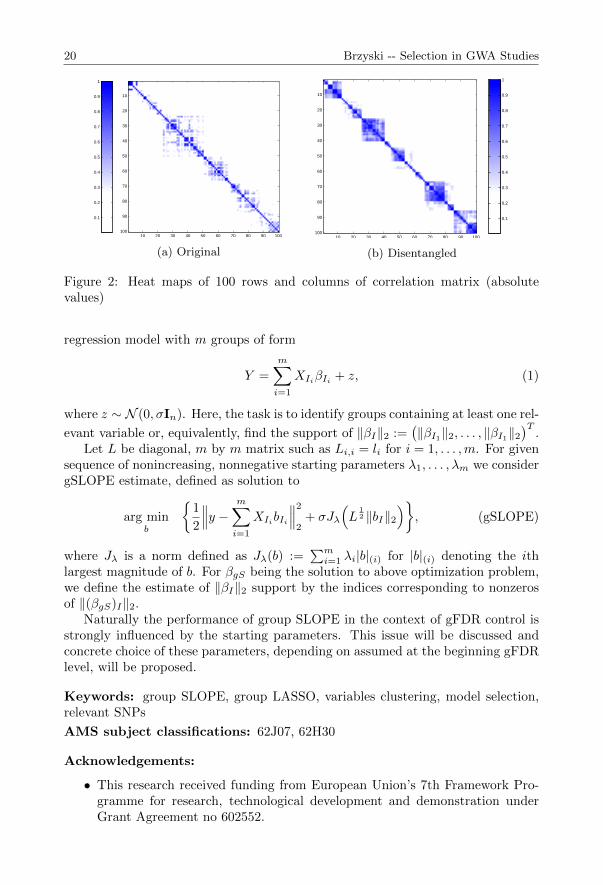
The method we used, group SLOPE, has been designed to transfer the SLOPEfalse discovery rate control property into groups level in situation when correla-tions between variables, included to different clusters, are weak. Under such cir-cumstances, grouping data based on the strength of the linearity between them isnatural procedure. Design matrices in GWA studies are structured in specific ways.There appears tendency of strong correlation between nearly located columns whilecolumns of distant indices are generally weakly correlated. The dependency is notobvious, however, and groups of strongly correlated covariates are mixed ratherthan located one after another. To ”disentangle” the explanatory variables, i.e. topermute them and cut into blocks corresponding to the various clusters, an algo-rithm based on hierarchical clustering (HCA) [2] was used. HCA clusters data usingthe similarity matrix which, in considered case, was defined based on correlationmatrix. In Figure 2 we present heatmaps of correlations matrices (absolute values)for original data (2a) and for disentangled variables (2b). Clearly noticeable, blockdiagonal structure of the latter shows that data were properly clustered.
Suppose that I = I1, . . . , Im is some partition of set 1, . . . , p defining thedivision of predictors into groups. Let li be the number of elements in group i fori = 1, . . . ,m. For a given data matrix, X ∈ M(n, p), we will consider the linear
20 Brzyski -- Selection in GWA Studies
10 20 30 40 50 60 70 80 90 100
10
20
30
40
50
60
70
80
90
100
0.1
0.2
0.3
0.4
0.5
0.6
0.7
0.8
0.9
1
(a) Original
10 20 30 40 50 60 70 80 90 100
10
20
30
40
50
60
70
80
90
100
0.1
0.2
0.3
0.4
0.5
0.6
0.7
0.8
0.9
1
(b) Disentangled
Figure 2: Heat maps of 100 rows and columns of correlation matrix (absolutevalues)
regression model with m groups of form
Y =
m∑i=1
XIiβIi + z, (1)
where z ∼ N (0, σIn). Here, the task is to identify groups containing at least one rel-
evant variable or, equivalently, find the support of ‖βI‖2 :=(‖βI1‖2, . . . , ‖βI1‖2
)T.
Let L be diagonal, m by m matrix such as Li,i = li for i = 1, . . . ,m. For givensequence of nonincreasing, nonnegative starting parameters λ1, . . . , λm we considergSLOPE estimate, defined as solution to
arg minb
1
2
∥∥∥y − m∑i=1
XIibIi
∥∥∥2
2+ σJλ
(L
12 ‖bI‖2
), (gSLOPE)
where Jλ is a norm defined as Jλ(b) :=∑mi=1 λi|b|(i) for |b|(i) denoting the ith
largest magnitude of b. For βgS being the solution to above optimization problem,we define the estimate of ‖βI‖2 support by the indices corresponding to nonzerosof ‖(βgS)I‖2.
Naturally the performance of group SLOPE in the context of gFDR control isstrongly influenced by the starting parameters. This issue will be discussed andconcrete choice of these parameters, depending on assumed at the beginning gFDRlevel, will be proposed.
Keywords: group SLOPE, group LASSO, variables clustering, model selection,relevant SNPs
AMS subject classifications: 62J07, 62H30
Acknowledgements:
• This research received funding from European Union’s 7th Framework Pro-gramme for research, technological development and demonstration underGrant Agreement no 602552.

Proceedings of the 19th EYSM in Prague 2015 21
• This article uses data from Northern Finland Birth Cohort 1966 (NFBC1966).
References
[1] M. Bogdan, R. van den Berg, W. Su, E. J. Candes. Statistical Estimation andTesting via the Ordered `1 Norm.
[2] Johnson S. C. Hierarchical clustering schemes. Psychometrika, Vol. 32, 241–254,1967.
[3] Yuan M., Lin Y. Model selection and estimation in regression with groupedvariables. Journal of the Royal Statistical Society, Series B, 68(1):49-67, 2007.
[4] Yuan M., Lin Y. Consistent group selection in high-dimensional linear regres-sion. Bernoulli, 16(4):1369-1384, 2007.
[5] Noah Simon, Jerome Friedman, Trevor Hastie, Rob Tibshirani A sparse-grouplasso. Journal of Computational and Graphical Statistics, 2013.
[6] By Peng Zhao, Guilherme Rocha, Bin Yu The composite absolute penaltiesfamily for grouped and hierarchical variable selection. Annals of Statistics,37(6A):3468-3497, 2009.
[7] Howard D. Bondell, Brian J. Reich Simultaneous regression shrinkage, variableselection and clustering of predictors with OSCAR. Biometrics, 64(1):115–23,2008.
[8] Guillaume Obozinski, Ben Taskar, Michael I. Jordan Joint covariate selectionand joint subspace selection for multiple classification problems. Statistics andComputing, 20(2):231–252, 2010.

Experience with Linear Programming forExperimental Design
Katarına Burclova∗1 and Andrej Pazman1
1Department of Applied Mathematics and Statistics, Faculty of Mathematics,Physics and Informatics, Comenius University, Bratislava, Slovakia
Abstract: In [4, 3] is proposed a method for computing optimal experimental de-sign via linear programming (LP) as a modification of method of cutting planes [2].We extend these results to a larger set of optimality criteria. The main idea is torewrite the concave, positive homogeneous optimality criterion φ in a form:
φ(ξ) = minµ∈Ξ
∑x∈X
H(µ, x)ξ(x), (1)
with a given function H(·; ·), ξ ∈ Ξ, the set of all probability measures on X , whereX is supposed to be finite design space. This reformulation allows us to interpret theproblem of finding optimal design ξ∗ = arg maxξ∈Ξ φ(ξ) by the iterative algorithmwhich solves an LP problem at each iteration. For the criteria of D- and A-optimality and for the class of Ek criteria we obtained the required formula (1)using standard algebraic relations.
The proposed algorithm contains a stopping rule, but also the standard stoppingrules following from the equivalence theorem can be used. The chief advantage ofthe algorithm is the possibility of combining optimality criteria or adding somesupplementary (cost) constraints linear in ξ. By modifying the algorithm we caneasily compute e.g. a D-optimal design under the condition that the A-optimalitycriterion attains a prescribed value a. Moreover, the computationally difficultproblem of the “criterion robust” design (cf. [1]) can be approached by the LPmethod.
Keywords: optimum design, optimality criteria, cutting-plane method, cost con-straints
AMS subject classifications: 62K05, 90C05
References
[1] R. Harman. Minimal efficiency of designs under the class of orthogonally in-variant information criteria. Metrika, 60:137–153, 2004.
[2] J. Kelley. The cutting plane method for solving convex programs. Journal ofthe Society for Industrial and Applied Mathematics, 8(4):703–712, 1960.
[3] A. Pazman, and L. Pronzato. Optimum design accounting for the global non-linear behavior of the model Annals of Statistics, 42(4):1426–1451, 2014.
∗Corresponding author: [email protected]

Proceedings of the 19th EYSM in Prague 2015 23
[4] L. Pronzato, and A. Pazman. Design of Experiments in Nonlinear Mod-els. Asymptotic Normality, Optimality Criteria and Small-Sample Properties.Springer, 2013.

Propensity Score Matching with Clustered Data
Massimo Cannas∗1 and Bruno Arpino2
1University of Cagliari, Italy2Pompeu Fabra University, Barcelona, Spain
Abstract: This paper focuses on the implementation of propensity score match-ing for clustered data. Different approaches to reduce bias due to cluster-levelconfounders are considered and compared using Monte Carlo simulations. We in-vestigated methods that exploit the clustered structure of data in two ways: inthe estimation of the propensity score model (through the inclusion of fixed orrandom effects) or in the implementation of the matching algorithm. In additionto a pure within-cluster matching, we also assessed the performance of a “pref-erential” within-cluster matching. This approach first searches for control unitsto be matched to treated units within the same cluster. If matching is not pos-sible within-cluster, then the algorithm searches in other clusters. The preferen-tial within-cluster matching approach, combining the advantages of within- andbetween-cluster matching, showed a relatively good performance both in the pres-ence of big and small clusters and it was often t he best method.
Keywords: causal inference, hierarchical data, propensity score matching
1 Introduction
In observational studies, direct comparison of outcomes across treatment groupscan give rise to biased estimates because groups being compared may be differentdue to lack of randomization. Subjects with certain characteristics may have higherprobabilities than others to be exposed to the treatment. If these characteristicsare also related to the outcome under investigation, an unadjusted comparison ofthe groups is likely to produce wrong conclusions about the treatment effect.
Propensity scores, defined as the probability to receive the treatment conditionalon the set of observed variables, were introduced by Rosenbaum and Rubin [4] asa one-dimensional summary of the multidimensional set of covariates, such thatwhen the propensity scores are balanced across the treatment and control groups,the distribution of all covariates are balanced across the two groups. In this waythe problem of adjusting for a multivariate set of observed characteristics reducesto adjusting for the one-dimensional propensity score. (See Austin [1] for a reviewon the use of propensity score methods in the medical literature).
In this paper, we focus on propensity score matching and consider differentapproaches to take into account the clustered structure of the data with the aimof reducing the bias due to cluster-level confounders. We consider methods thatexploit the information on the clusters to which units belong in two ways: in the
∗Corresponding author: [email protected]

Proceedings of the 19th EYSM in Prague 2015 25
estimation of the propensity score model via the inclusion of fixed or random effects;in the implementation of the matching algorithm.
When clusters sizes are big enough, within-cluster matching is a valid strategybut it can still imply the lost of many units that cannot find a match because thesearch is forced to be within clusters [2]. Discarding unmatched units is problem-atic because it may imply a change of the estimand [3]. In addition to a purewithin-cluster matching, we also propose and assess the performance of an ap-proach that has not been tested in previous studies. This approach first searchesfor control units to be matched to treated units within the same cluster. If match-ing is not possible within-cluster, then the algorithm searches in other clusters.This approach, that we define ‘preferential’ within-cluster matching, is expected tocarry the benefits of pure within-cluster matching (in terms of bias reduction) andmatching on the pooled dataset (in terms of minimizing the number of unmatchedunits).
2 Background
Consider a two-level data structure where N individual-level units, indexed by i(i = 1, 2, ..., nj), are nested in J second-level units (clusters), indexed by j (j =1, 2, ..., J). We consider a binary treatment administered at the individual level,T , and an outcome variable, Y also measured at the individual level. Confounderscan be first (X) or second-level (Z) variables.
Usually, the Average Treatment effect on the Treated (ATT) is considered as aninteresting summary of individual causal effects: ATT = E(Yij(1) − Yij(0) |Tij =1). To identify the ATT with observational data, the following assumptions areoften invoked:
• Unconfoundedness: Y (1), Y (0) ⊥ T |(X,Z);
• Overlap: 0 < P (T = 1 | (X,Z)) < 1.
Under the previous assumptions, adjustment on the propensity score is sufficientto eliminate bias due to observed confounders [4]. The propensity score, e, is definedfor each unit as the probability to receive the treatment given its covariate values:eij = P (Tij = 1 | (Xij , Zj)). Rosenbaum and Rubin [4] proved that the propensityscore is a balancing score, i.e., (X,Z) ⊥ T | e(X,Z), meaning that at each valueof the propensity score the distribution of the covariates defining the propensityscore is the same in the treated and control groups. They also showed that ifunconfoundedness holds conditioning on covariates it also holds conditioning on thepropensity score, i.e., Y (1), Y (0) ⊥ T | e(X,Z). These results justify adjustmenton the propensity score instead of on the full multivariate set of covariates.
Usually, in observational studies the propensity score is not known and must beestimated from the data. Parametric models, such as logit or probit models, withinclusion of interactions and higher order terms are commonly used. An incorrectlyestimated propensity score may fail to respect the balancing property. Our focusis not on misspecification of the functional form of the propensity score model buton the bias caused by omitted cluster-level confounders. If one or more variables

26 Cannas and Arpino -- Propensity Score Matching with Clustered Data
affecting the selection into treatment and potential outcomes are not observed, thenunconfoundedness is violated and ATT estimators based on the propensity scorewill be biased. the foll owing can be adapted when some observed cluster-levelvariables are observed and others are not.
Among propensity score methods available to adjust for an unbalanced distribu-tion of covariates between treated and control groups, we consider propensity scorematching (PSM). In particular, we consider one-to-one nearest neighbor matchingwithin a maximum distance (caliper) of 0.20 standard deviations of the estimatedpropensity score. For each treated unit in the sample, the algorithm searches forthe closest control unit in terms of propensity score. If no control unit is availablein the range defined by the caliper, the treated unit is discarded from the workingsample. We considered matching with replacement, where the same control unitcan be used several times as a match. Matching with replacement is expected toimprove the quality of matches and therefore to reduce bias [8]. However, a bias-variance trade-off emerges because matching with replacement increases varianceof estimates [9]. Since our main focus is on the bias of the estimators we consideredmatching with replacement.
When the dataset has a 2-level structure one can consider different ways ofimplementing PSM. The methods we compare are as follows:
A) Single-level propensity score model; matching on the pooled dataset;
B) Single-level propensity score model; within-cluster matching;
C) Single-level propensity score model; preferential within-cluster matching;
D) Random-effects propensity score model; matching on the pooled dataset;
E) Fixed-effects propensity score model; matching on the pooled dataset.
3 Simulation scenario
In this section we describe our simulation experiments aimed at comparing theperformance of the different matching strategies described above in the presence ofunobserved confounders at the cluster-level.
3.1 Set-up
We designed our simulation experiments to mimic the observed data in severalrespects. First, we kept the same data structure observed in our dataset, i.e. thesame number of clusters (hospitals) and the same clusters’ sample sizes (see Table1). In this way, in our simulations we consider a realistic case with a stronglyunbalanced structure where some clusters are big and others have small samplesizes. Second, instead of generating values of covariates as realizations of randomvariables as typically done in simulation studies, we used the same covariates dis-tribution as observed in the dataset. The only exception was for a cluster-levelvariable, Z, that we introduce to explore the confounding effect at the cluster (i.e.,hospital) level. Finally, the coefficients of individual-level covariates in the true
Proceedings of the 19th EYSM in Prague 2015 27
models generating the treatment and the outcome were set to values similar toobserved coefficients estimated on the real data.
Given the complete set of covariates (X,Z) the probability of being treated wasgenerated according to:
eij = 1/[1 + exp(β0 + β1X1ij + · · ·+ βkXkij + βk+1Zj)] (1)
and the outcome was generated by the following model:
P (Yij = 1) = 1/[1 + exp(γ0 + γ1X1ij + · · ·+ γkXkij + γk+1Zj + αTij)], (2)
where β = [β0, · · ·βk+1] and γ = [γ0, · · · γk+1] are the vectors of coefficients,X = (X1, · · ·Xk) is the set of observed individual-level confounders and Z is thecluster-level confounder. Values of Z are generated as realizations of a normalvariable with µZ = 0 and σZ = 0.25, which is equal to the average standarddeviation of the observed confounders.
Under each scenario, 500 datasets were generated from models (1) and (2). Foreach simulated dataset we employed the PSM methods described in the previoussection to obtain a matched subset. The simulation experiments were implementedin R [10]. In particular, for methods A, D and E we obtained the matched subsetsusing the function Match in the package Matching [7]. At the time of writingneither this package nor others have an option for implementing within-cluster(B) and preferential within-cluster matching (C) so we programmed a routine thatmakes use of the Match function (the code is available from the authors uponrequest).
We summarized the results by averaging over the 500 replicates the followingmetrics calculated on each dataset: the number and the percentage of unmatchedtreated units, the absolute standardized bias (ASB) of each confounder, the esti-
mated treatment effect (ATT ), the percent bias of the estimated effect (%BIAS)and the squared error (SE).
4 Results
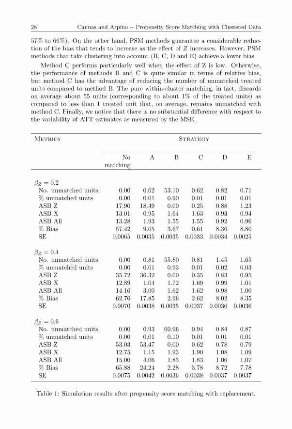
Table 1 presents the results of the baseline simulation study introduced in theprevious section. We considered three scenarios by varying the effect of the hospital-level unobserved confounder in the true treatment assignment model, that is βZ =0.2, 0.4, 0.8. For each scenario, we compare the performance of the five PSMstrategies described in section 3 (A-E) in terms of unmatched units, balance (ASB),percent bias and mean squared error (MSE). We also report in the first column theresults obtained without any adjustment (“no matching”).
In general, we notice that an unadjusted comparison between treated and con-trol groups’ outcomes gives strongly biased estimates (relative bias ranging from
28 Cannas and Arpino -- Propensity Score Matching with Clustered Data
57% to 66%). On the other hand, PSM methods guarantee a considerable reduc-tion of the bias that tends to increase as the effect of Z increases. However, PSMmethods that take clustering into account (B, C, D and E) achieve a lower bias.
Method C performs particularly well when the effect of Z is low. Otherwise,the performance of methods B and C is quite similar in terms of relative bias,but method C has the advantage of reducing the number of unmatched treatedunits compared to method B. The pure within-cluster matching, in fact, discardson average about 55 units (corresponding to about 1% of the treated units) ascompared to less than 1 treated unit that, on average, remains unmatched withmethod C. Finally, we notice that there is no substantial difference with respect tothe variability of ATT estimates as measured by the MSE.
Metrics Strategy
No A B C D Ematching
βZ = 0.2No. unmatched units 0.00 0.62 53.10 0.62 0.82 0.71% unmatched units 0.00 0.01 0.90 0.01 0.01 0.01ASB Z 17.90 18.49 0.00 0.25 0.88 1.23ASB X 13.01 0.95 1.64 1.63 0.93 0.94ASB All 13.28 1.93 1.55 1.55 0.92 0.96% Bias 57.42 9.05 3.67 0.61 8.36 8.80SE 0.0065 0.0035 0.0035 0.0033 0.0034 0.0025
βZ = 0.4No. unmatched units 0.00 0.81 55.80 0.81 1.45 1.65% unmatched units 0.00 0.01 0.93 0.01 0.02 0.03ASB Z 35.72 36.32 0.00 0.35 0.83 0.95ASB X 12.89 1.04 1.72 1.69 0.99 1.01ASB All 14.16 3.00 1.62 1.62 0.98 1.00% Bias 62.76 17.85 2.96 2.62 8.02 8.35SE 0.0070 0.0038 0.0035 0.0037 0.0036 0.0036
βZ = 0.6No. unmatched units 0.00 0.93 60.96 0.94 0.84 0.87% unmatched units 0.00 0.01 0.10 0.01 0.01 0.01ASB Z 53.03 53.47 0.00 0.62 0.78 0.79ASB X 12.75 1.15 1.93 1.90 1.08 1.09ASB All 15.00 4.06 1.83 1.83 1.06 1.07% Bias 65.88 24.24 2.28 3.78 8.72 7.78SE 0.0075 0.0042 0.0036 0.0038 0.0037 0.0037
Table 1: Simulation results after propensity score matching with replacement.

Proceedings of the 19th EYSM in Prague 2015 29
Acknowledgements: We would like to thank the Autonomous Region of Sar-dinia for providing the anonymized data used in the empirical application.
References
[1] Austin PC. A critical appraisal of propensity score matching in the medicalliterature between 1996 and 2003. Statistics in medicine, 27(12): 2037-2049,2008.
[2] Gayat E, Thabut G, Christie JD, Mebazaa A, Mary JY and R Porcher. Within-center matching performed better when using propensity score matching toanalyze multicenter survival data: empirical and Monte Carlo studies. Journalof clinical epidemiology, 66(9): 1029-1037, 2013.
[3] Crump RK, Hotz VJ, Imbens GW, Mitnik O. Dealing with limited overlap inestimation of average treatment effects. Biometrika, 96:187-195, 2009.
[4] PR, Rosenbaum, and DB Rubin. The central role of the propensity score inobservational studies for causal effects. Biometrika, 70: 41-55, 1982.
[5] Arpino B, Mealli F. The specification of the propensity score in multilevelobservational studies. Computational Statistics and Data Analysis, 55: 1770-1780, 2011.
[6] Thoemmes FJ, West SG. The use of propensity scores for nonrandomizeddesigns with clustered data. Multivariate Behavioral Research, 46(3): 514-543,2011.
[7] Sekhon JS. Multivariate and Propensity Score Matching Software with Au-tomated Balance Optimization. Journal of Statistical Software, 42(7): 1-52,2011.
[8] EA Stuart Matching methods for causal inference: A review and a look forward.Statistical science: a review journal of the Institute of Mathematical Statistics,25(1): 1, 2010.
[9] Caliendo M, Kopeinig S. Some practical guidance for the implementation ofpropensity score matching. Journal of economic surveys 2008; 22(1): 31-72.
[10] R Core Team (2014). R: A language and environment for statistical computing.R Foundation for Statistical Computing. URL http://www.R-project.org/.
Estimating Whole Brain Dynamics Using SpectralClustering
Ivor Cribben1 and Yi Yu∗2
1Department of Finance and Statistical Analysis, Alberta School of Business,Canada
2Statistical Laboratory, University of Cambridge, UK
Abstract: Recently, in functional magnetic resonance imaging (fMRI), there hasbeen an increased interest in quantifying changes in connectivity between brainregions over an experimental time course to provide a deeper insight into the fun-damental properties of brain networks. The application of graphical and networkmodelling has been instrumental in these analyses and has enabled the examinationof the brain as an integrated system. In this work, we propose a new statisticalmethod to provide important insights into the time-varying nature of the connec-tivity of brain regions while subjects are at rest. The novel method uses spectralclustering to study the network structure between brain regions and uses a non-parametric metric to detect the change in the structures across time course. Thenew method allows for situations where the number of brain regions is greater thanthe number of time points in the experimental time course (n < p). This methodpromises to offer deeper insight into the inner workings of the whole brain. Weapply this new method to simulated data and to a resting-state fMRI data set.The temporal features of this novel connectivity method will provide a more ac-curate understanding of the large-scale characterisations of brain disorders such asAlzheimers disease and may lead to better diagnostic and prognostic indicators.
∗Corresponding author: [email protected]

On the Estimation of the Central Core of a Set.Algorithms to Estimate the λ-Medial Axis
Antonio Cuevas1, Pamela Llop2 and Beatriz Pateiro-Lopez∗3
1Universidad Autonoma de Madrid, Spain2Facultad de Ingenierıa Quımica (UNL) and Instituto de Matematica Aplicada
del Litoral (UNL - CONICET), Argentina3Universidad de Santiago de Compostela, Spain
Abstract: The medial axis and the inner parallel body of a set C in the Euclideanspace are different formal translations for the notions of the “central core” and the“bulk”, respectively, of C. On the basis of their applications in image analysis, bothnotions (and especially the first one) have been extensively studied in the literature,from different points of view. A modified version of the medial axis, called λ-medialaxis, has been recently proposed in order to get better stability properties. Theestimation of these relevant subsets from a random sample of points is a partiallyopen problem which has been considered only very recently. Our aim is to showthat standard, relatively simple, techniques of set estimation can provide natural,consistent, easy-to-implement estimators for both the λ-medial axis Mλ(C) andthe inner parallel body Iλ(C) of C. The consistency of these estimators followsfrom two results of stability (i.e. continuity in the Hausdorff metric) ofMλ(C) andIλ(C) obtained under some, not too restrictive, regularity assumptions on C. Asa consequence, natural algorithms for the approximation of the λ-medial axis andthe λ-inner parallel body can be derived. The whole approach could be useful forsome practical problems in image analysis where estimation techniques are needed.
Keywords: medial axis, set estimation, r-convexity
AMS subject classifications: 62G05
1 Introduction
There is a rich mathematical literature devoted to the study of the “central part”of a set C in the Euclidean space (which would represent, in statistical terms, the“median of C”); see [1]. Of course, the first step in any such study must be togive a precise meaning to this loose notion of “set median”. Different definitions,closely related but not always equivalent, have been proposed. The most popularone is perhaps the medial axis of C, M(C), defined as the subset of points in Chaving at least two projections on the boundary ∂C. Other closely related (but notequivalent) usual notions are the skeleton , S(C), (the set of centers of maximalballs included in C) and the cut locus of C, defined as the topological closure ofM(C); see below for further discussion on these notions. The medial axis was
∗Corresponding author: [email protected]

32 Cuevas, Llop and Pateiro-Lopez -- Algorithms to Estimate the λ-Medial Axis
introduced by [2] as a tool in image analysis. The papers by [4], [3] and [5], amongmany others, analyze these ideas from different points of view.
We are especially concerned with a modified version of the medial axis, calledλ-medial axis, Mλ(C), introduced in [3] to deal with the well-known problem ofinstability in the medial axis: the medial axisM(C) andM(D) might be far awayfrom each other even if the original sets C and D and their boundaries are veryclose together; see [4] and references therein. The λ-medial axis leaves out thosepoints of M(C) whose metric projections on ∂C are too close together.
Another, perhaps less popular, closely related concept is the so-called λ-innerparallel body, Iλ(C), defined as the set of points in C whose distance to ∂C is atleast λ. So far this concept has been mainly studied in the case where C is convex[see, e.g., [8]] but we will see that this assumption is not necessary to find a simpleconsistent estimator of Iλ(C). The λ-inner parallel body has a simple intuitiveinterpretation and is obviously close to the notion of “core” of C. In some casesit provides an outer approximation to the λ-medial axis. The algorithm proposedin the paper by [7] for medial axis estimation (under a regression-type samplingmodel) relies on an estimate of the inner parallel set.
This work deals with the statistical problem of estimating the λ-medial axis,Mλ(C), and the λ-inner parallel body, Iλ(C), from a random sample of pointsX1, . . . , Xn drawn inside C. The whole approach relies on a simple plug-in idea:we will use methods of set estimation (see, e.g., [6] for a survey) to get a suitableestimator Cn = Cn(X1, . . . , Xn) of C. Then the natural estimators ofMλ(C) andIλ(C) would be just Mλ(Cn) and Iλ(Cn), respectively.
Whereas the theoretical and practical aspects of the medial axis (and associatednotions) have received a considerable attention, the problem of estimating this sethas been considered only very recently: we refer to the recent paper by [7], thoughthe sampling model considered by these authors is a bit different to that we willuse here. In short, we will show that imposing an additional shape restriction on C(called r-convexity) one can obtain, in return, a considerable simplification in thetheory and practice of the estimation of Mλ(C) and Iλ(C).
Acknowledgements: This work has been partially supported by Spanish GrantMTM2013-41383P from Ministry of Economy and Competitiveness, European Re-gional Development Fund (ERDF) and the IAP research network grant no. P6/03from the Belgian government (third author).
References
[1] Attali, D., Boissonnat, J.-D. and Edelsbrunner, H. Stability and Computationof Medial Axis: a State-of-the-Art Report. In Mathematical Foundations ofScientific Visualization, Computer Graphics, and Massive Data Exploration, T.Moeller, B. Hamann and R. Russell, eds., pp 109–125. Springer-Verlag, Berlin,2009.
[2] Blum, H. A Transformation for Extracting New Descriptors of Shape. In W.Wathen-Dunn, editor, Models for the Perception of Speech and Visual Form,Cambridge, MA, MIT Press, 362–380, 1967.

Proceedings of the 19th EYSM in Prague 2015 33
[3] Chazal, F. and Lieutier, A. The “λ-medial Axis”. J. Graphical Models, 67:304–331, 2005.
[4] Chazal, F. and Soufflet, R. Stability and Finiteness Properties of Medial Axisand Skeleton. J. Dynam. Control Systems, 10:149–170, 2004.
[5] Chaussard, J., Couprie, M and Talbot, H. Robust Skeletonization Using theDiscrete λ-medial Axis. Pattern Recognition Letters, 32:1384–1394, 2011.
[6] Cuevas, A. and Fraiman, R. Set Estimation. In New Perspectives on StochasticGeometry, W.S. Kendall and I. Molchanov, eds., pp. 374–397. Oxford UniversityPress, 2010.
[7] Genovese, C.R., Perone-Pacifico, M., Verdinelli, I. and Wasserman, L. TheGeometry of Nonparametric Filament Estimation. J. Amer. Statist. Assoc.,107:788–799, 2012.
[8] Sangwine-Yager, J.R. Bonnesen-style Inequalities for Minkowski Relative Ge-ometry. Trans. Amer. Math. Soc., 307:373–382, 1988.
Model Fitting for Space-Time Point PatternsUsing Projection Processes
Jirı Dvorak∗12
1Department of Probability and Mathematical Statistics, Faculty of Mathematicsand Physics, Charles University in Prague, Czech Rep.
2Department of Image Processing, Institute of Information Theory andAutomation, The Czech Academy of Sciences, Czech Rep.
Abstract: Statistical inference for spatial and space-time point patterns recordede.g. in ecological or epidemiological applications represents a challenging task. Thedata consists of a random collection of points u1, . . . , uN observed in a compactobservation window W , or, in the space-time setting, a random collection of space-time events (u1, t1), . . . , (uN , tN ) observed in W over a time period T . Both thenumber of observed points N and their locations are random.
We focus our attention on the space-time clustered point patterns. We discussthe possibility to use dimension-reduction techniques to fit different parts of a space-time model separately. Specifically, we define the projections of the process to thespatial and temporal domain, respectively, and introduce a step-wise estimationprocedure based on these projections. We also discuss the problem of possiblecluster overlapping and the resulting loss of information in the projections and thechallenges it presents for parameter estimation.
Keywords: space-time point process, Cox process, minimum contrast estimation,K-function, projection process
AMS subject classifications: 62M30, 60G55
1 Introduction
Many fields of science deal with data that are point patterns, such as positions oftrees in a rain forest, maps of disease cases or the locations of point-like defects inindustrial materials. A point pattern consists of a finite set of points u1, . . . , uNobserved in a compact observation window W ⊂ Rd. Figure 1 provides an exampleof different point patterns. A random process generating such point patterns iscalled a point process. Formally speaking, a point process X in Rd is a measurablemapping from an abstract probability space to the space of locally finite subsetsof Rd. This implies that the number N of points of X ∩W is a random variable.Also, the locations of the points are random.
The necessity to analyse point patterns arising in practical applications leadto significant development of the point process theory in the past decades. Fora comprehensive review see [2, 4] or [5]. Parametric point process models enabledetailed statistical inference and hence are sought for in practice.
∗Corresponding author: [email protected]

Proceedings of the 19th EYSM in Prague 2015 35
Figure 1: Examples of different point patterns. Left: the locations of the centersof 42 biological cells observed under optical microscopy in a histological section.Middle: simulated realization of a Poisson point process (see the text). Right:the locations of 62 seedlings and saplings of California redwood trees in a squaresampling region. The two real point patterns are standard datasets available inthe spatstat package [1] for R.
The basic point process model is the Poisson process. Consider a non-negativefunction λ(u), u ∈ Rd. The point process X is called the Poisson process withintensity function λ if the number of points of X in a Borel set B ⊂ Rd hasa Poisson distribution with mean
∫Bλ(u) du and the point counts in disjoint Borel
sets are independent random variables. This model exhibits no interaction betweenpoints. For a sample realization see the middle panel of Figure 1.
A natural generalization of the Poisson process is the Cox process. Let Λ(u), u ∈Rd, be a non-negative random field such that u 7→ Λ(u) is a locally integrablefunction with probability 1. If the conditional distribution of the point process Xgiven Λ = λ is the distribution of the Poisson process with intensity function λ,X is said to be the Cox process with the driving field Λ [4]. A Cox process isthe model of choice when it comes to analysis of clustered point patterns (such asthe one in the right panel of Figure 1) as it is able to accomodate the attractiveinteractions among the points. However, Cox process models are not suitable formodelling regular patterns such as the one in the left panel of Figure 1.
In this contribution we will focus on the problem of model fitting for clusteredspace-time point patterns. In this case each point (sometimes also called event)of the space-time point process X has a spatial position u ∈ Rd and a temporalcoordinate t ∈ R. In the following we will use (u, t) ∈ X to denote that a pointof X occurs at location u at time t. We assume that the data is observed in acompact set W ×T ⊂ Rd×R with positive Lebesgue measure where W is a spatialregion observed over the time period T .
We emphasize that we consider a continuous time domain T (not discrete timeinstances) and that the events have no duration. Hence (u, t) ∈ X might e.g. in anepidemiological application correspond to an animal kept on a farm with location ubeing reported at time t to be infected.
Furthermore, we remark that analysis of space-time point patterns observed in

36 Dvorak -- Model Fitting for Space-Time Point Patterns
a compact subset of Rd × R requires dedicated methods. It is not appropriate touse methods for spatial point patterns in Rd+1 – the temporal coordinate playsa distinct role and cannot be interchanged with the spatial coordinates. For ex-ample, it is not natural to measure the difference between two space-time eventsusing the Eucliedean norm in Rd+1.
2 Background
For ease of exposition we restrict our attention to stationary point processes, i.e. theprocesses with translation invariant distribution. At first we present the necessarydefinitions in the spatial setting and then extend them to the space-time setting.We also assume that the point process in question is simple, i.e. two points cannotoccur at the same location. For further details [2] can be consulted.
Let X be a stationary point process in Rd. If B is a Borel set in Rd we denoteby |B| its volume and by X(B) the number of points of X in B. The intensity ρof X is defined as the expected number of points of X in a set of unit volume, i.e.ρ = EX(B)/|B| for B with positive volume and ρ does not depend on the choiceof B. We assume ρ > 0.
Furthermore, let du be an infinitesimal region containing the point u ∈ Rd. Thesecond-order intensity function of X is defined by
ρ2(u, v) = lim|du|,|dv|→0
E [X(du)X(dv)]
|du| |dv| .
For u 6= v, ρ2(u, v) |du| |dv| can be regarded as the approximate probability thatdu and dv both contain a point of X. From the assumption of stationarity of Xwe see that, with a slight abuse of notation which is common in the field of spatialstatistics, ρ2(u, v) = ρ2(0, v − u) = ρ2(v − u).
Useful point process characteristics are the pair-correlation function g(u) =ρ2(u)/ρ2, u ∈ Rd, and the K-function defined by
K(r) =
∫B(o,r)
g(w) dw, r > 0,
where B(o, r) is the ball centered at the origin o with radius r. We remark thatthe value ρK(r) can also be interpreted as the mean number of points from X inB(o, r) \ o provided that there is a point of X in o.
Now we can extend our definitions to the space-time setting. We keep trackof the temporal coordinate of points by explicitely writing (u, t) ∈ Rd × R. Itis straightforward to define the space-time intensity, second-order intensity func-tion and the space-time pair-correlation function in the same way as above. Nowρ2((u, t), (v, s)) = ρ2(v − u, s− t) = ρ2g(v − u, s− t).
The definition of the space-time K-function must take into account the principaldifference between the spatial and temporal coordinates. Hence we define
K(r, t) =
∫B(o,r)
∫ t
−tg(w, τ) dτ dw, r > 0, t > 0,

Proceedings of the 19th EYSM in Prague 2015 37
as a function of two arguments – the spatial distance r and the temporal lag t. NowρK(r, t) can be interpreted as the mean number of points from X in the cylinder(B(o, r)× [−t, t]) \ (o, o) provided that there is a point of X in (o, o).
3 Model fitting
While the extent of this contribution does not allow us to specify the model indetail, we have in mind the shot-noise Cox processes [4]. They constitute a wideand flexible class of models for clustered point patterns. In what follows it is crucialthat the model allows the separation of the first-order parameters (intensity ρ > 0)and interaction parameters (possibly a vector parameter ψ of the pair-correlationfunction g(u, t;ψ)). The model is fully parametrized by (ρ, ψ).
For a general Cox point process it is very difficult to obtain maximum likeli-hood estimate of the model parameters. The reason is that the likelihood involvesan expectation of a complicated integral term with respect to the distribution ofthe random driving field Λ. One can of course take advantage of MCMC or othertechniques and use approximations of the likelihood function [4]. This approach isusually computationally very demanding and thus faster, simulation-free alterna-tives based on moment properties are preferred.
For a space-time shot-noise Cox process there is an explicit expression for thespace-time K-function K(r, t;ψ). The non-parametric estimate of the space-timeK-function is
K(r, t) =1
(ρ)2 |W × T |
6=∑(ui,ti),(uj ,tj)∈X∩(W×T )
I(‖ui − uj‖ ≤ r, |ti − tj | ≤ t)w1(ui, uj)w2(ti, tj)
,
where I is the indicator function, ‖·‖ denotes the Euclidean norm in Rd, w1, w2
are the spatial and temporal edge-correction factors [3], ρ = X(W ×T )/|W ×T | isthe natural non-parametric estimate of the intensity ρ and the summation is overdistinct pairs of points of X.
Now we can use the classical minimum contrast method to find the estimate ofthe interaction parameters ψ by minimizing the discrepancy∫ rmax
rmin
∫ tmax
tmin
(K(r, t)q −K(r, t;ψ)q)2 dtdr,
for some bounds 0 < rmin < rmax and 0 < tmin < tmax. Here q is a variancestabilizing coefficient adjusting for the non-constant variance of K(r, t). Typicalvalues of q are 1/4 or 1/2.
However, this approach requires rather large amount of data in order to obtainstable estimates of K(r, t). Based on the idea used in [3] we proposed in [6] to definethe projections of the space-time process X to the spatial and temporal domain,respectively, and use these projections for estimation. We define
Xs = u : (u, t) ∈ X, t ∈ T,Xt = t : (u, t) ∈ X,u ∈W,

38 Dvorak -- Model Fitting for Space-Time Point Patterns
y
x
t
x
y
t
Figure 2: A sample realization of a space-time point process observed in W × T =[0, 1]2× [0, 1] (upper left) together with the corresponding spatial projection (upperright) and temporal projection (below).
i.e. when defining the spatial projection process Xs we keep only the points occur-ing in the time period T and then disregard their temporal coordinate. Similarlyfor the temporal projection process Xt. For a graphical illustration see Figure 2.
In [6] we consider space-time shot-noise Cox processes and we require an addi-tional assumption of a certain type of second-order separability. It in fact specifiesthat the (vector) interaction parameter ψ = (ψs, ψt) involves a spatial interactionparameter ψs and a temporal interaction parameter ψt and that the space-timeK-function K(r, t) of the process X depends in a separable way on the spatial part(depending only on ψs and r) and the temporal part (depending only on ψt and t).
Under this assumption it is possible to derive explicit formulae for the K-function Ks(r;ψs) of the projection process Xs and Kt(τ ;ψt) of Xt, respectively.Then Ks and Kt can be estimated non-parametrically and we can use minimumcontrast estimation based on Ks in order to estimate ψs and, similarly, minimumcontrast estimation based on Kt in order to estimate ψt. In this way the interactionparameters are estimated separately and, more importantly, the non-parametricestimates of Ks and Kt are more stable because by projecting we have reduced thedimension of the corresponding space.

Proceedings of the 19th EYSM in Prague 2015 39
4 Challenges
An interesting problem is caused by possible overlapping of clusters of points inthe data. Even clusters which were originally clearly separated in the space-timedomain may overlap in the spatial or temporal projection, making it more difficultto estimate the interaction parameters. This problem is more pronounced in thetemporal projection process where we project from Rd × R to R only.
A consequence of the cluster overlapping problem is that increasing the amountof observed data may not in general result in more precise estimates of the interac-tion parameters. Consider for example a fixed spatial domain W and an increasingsequence of time intervals Tn = [0, n]. If we use Tn to define a sequence of spatial
projection processes X(n)s , the intensity ρ
(n)s of X
(n)s would increase unboundedly.
This implies more and more cluster overlapping in X(n)s . It can be proved formally
that in the limit the influence of the spatial interaction parameter ψs is lost andit cannot be identified from Ks. The situation is analogous if we consider a fixedtime period T and an increasing sequence of spatial regions Wn.
This makes it difficult to find appropriate asymptotic regime for this estimationproblem and to formulate conditions under which consistency and asymptotic nor-mality of the resulting estimators hold. We conclude this contribution by a remarkthat it is in fact possible to formulate asymptotic results but different normalization
(by |Wn|1/2 or |Tn|1/2) is required for ψs and ψt, respectively.
Acknowledgements: The author would like to express his gratitude to his formersupervisor RNDr. Michaela Prokesova, Ph.D., for her never-ending enthusiasm,patience and support.
References
[1] A. Baddeley and R. Turner. Spatstat: An R package for analyzing spatial pointpatterns. Journal of Statistical Software, 12(6):1–42, 2005.
[2] J. Illian, A. Penttinen, H. Stoyan, and D. Stoyan. Statistical Analysis andModelling of Spatial Point Patterns. Wiley, 2008.
[3] J. Møller and M. Ghorbani. Aspects of second-order analysis of structured inho-mogeneous spatio-temporal point processes. Statistica Neerlandica, 66(4):472–491, 2012.
[4] J. Møller and R. P. Waagepetersen. Statistical inference and simulation forspatial point processes. Chapman & Hall/CRC, 2004.
[5] J. Møller and R. P. Waagepetersen. Modern statistics for spatial point processes.Scandinavian Journal of Statistics, 34(4):643–684, 2007.
[6] M. Prokesova and J. Dvorak. Statistics for inhomogeneous space-time shot-noise Cox processes. Methodology and Computing in Applied Probability,16(2):433–449, 2014.
The Evolving Evolutionary Spectrum
Mark Fiecas∗1 and Hernando Ombao2
1Department of Statistics, University of Warwick, Coventry CV4 7AL, UnitedKingdom
2Department of Statistics, University of California at Irvine, Bren Hall 2206,Irvine, CA 92697
Abstract: In this work, we developed a novel time series model in the context ofdesigned experiments that captures two sources of nonstationarities: 1) over timewithin a trial of the experiment and 2) across the trials of the experiment. Underthe proposed model we construct spectral measures that change with respect toboth sources of nonstationarities. To estimate the evolving evolutionary spectraldensity matrix, we used a two-stage procedure. In the first stage, we computed thewithin-trial time-localized periodogram matrix. In the second stage, we developeda data-driven approach for combining information across trials from the local pe-riodogram matrices. We assessed the performance of our proposed method usingsimulated data.
Keywords: multivariate time series, cross-coherence, local stationarity, spectralanalysis
AMS subject classifications: 62M10, 62P10
1 Introduction
The context of our work is in neuroscience experiments where nonstationary timeseries data are collected. Often in the experiment a stimulus is presented numeroustimes, and so the data set consists of a collection of many nonstationary multivari-ate time series across the trials of the experiment. However, existing methodologyfor spectral analysis of nonstationary time series data will assume that the dataacross the trials are identical realizations of the same underlying process. This isnot necessarily the case in practice. Indeed, the variability across trials may arisefrom the subject changing performance strategy, reduced neuronal activity poten-tially caused by habituation to the stimulus, or other neurophysiological processes[1, 2]. While many statistical models take into account nonstationarity within asingle trial, there is certainly a need for statistical methodologies to account for thenonstationarity over the course of the experiment in order to give a more accuratecharacterization of the underlying dynamics of the data.
∗Corresponding author: [email protected]

Proceedings of the 19th EYSM in Prague 2015 41
2 The evolving evolutionary spectrum
We begin with our statistical model that captures the two sources of nonstation-arities. Our modeling framework is inspired by the work of Dahlhaus (2000) [3]on locally stationary processes (LSP) but we go further by modeling the dynamicsacross an entire experiment rather than just within a single trial. The followingmodel was first developed by Fiecas and Ombao (2014) and used to study localfield potentials collected during an associative learning experiment [4]. We referthe reader to that work for more details and discussion.
Definition 1. A sequence of locally stationary zero-mean P -variate time series Xt,r
where r = 1, . . . , R denotes the trials within the entire experiment and t = 1, . . . , Tdenote the time points within a trial is said to follow a slowly evolving locallystationary process (SEv-LSP) if it admits the representation
Xt,r =
∫ 0.5
−0.5
A(t/T, r/R, ω) exp(i2πωt)dZr(ω),
where:
1. Zr(ω) is a zero-mean P -variate orthogonal increment process on [−0.5, 0.5]with Zr(ω) = Zr(−ω), Zr(ω) is uncorrelated with Zr′(ω) for r 6= r′, and
cum(dZr(ω1), . . . , dZr(ωk)) = η(
k∑j=1
ωj)Λk(ω1, . . . , ωk−1)dω1 · · · dωk,
where cum(·) denotes the k-th order cumulant, Λ1 = 0,Λ2 = IdP , where IdPis the P ×P identity matrix, |Λk(ω1, . . . , ωk−1)| ≤ Ck where Ck is a constant,Λ4 is continuous, and η(ω) =
∑∞j=−∞ δ(ω + j) is the periodic extension of
the Dirac delta function, and
2. For each (u, v, ω) ∈ [0, 1] × [0, 1] × [−0.5, 0.5], the complex-valued trans-fer function denoted A(u, v, ω) (of dimension P × P ) has continuous sec-ond partial derivatives with respect to u, v, and ω, and ∂lA(u, v, ω)/∂ωl =
∂lA(u, v,−ω)/∂ωl for l = 0, 1.
Definition 2. The evolving evolutionary spectral density matrix, with dimensionP × P , defined at rescaled time u ∈ [0, 1] within rescaled trial-time v ∈ [0, 1] andat frequency ω ∈ [−0.5, 0.5] is
f(u, v, ω) = A(u, v, ω)A(u, v, ω)∗,
where (*) denotes the conjugate transpose.
In spectral analysis, a popular approach for investigating the linear dependencebetween two time series is via cross-coherence analysis. Cross-coherence is analo-gous to cross-correlation but is frequency specific, i.e., it measures the strength oflinear association between two time series at a particular frequency.

42 Fiecas and Ombao -- The Evolving Evolutionary Spectrum
Definition 3. The evolving evolutionary coherence between dimensions p and q ofa SEv-LSP Xt,r is
ρ2pq(u, v, ω) =
∣∣∣∣∣ f(u, v, ω)pq√f(u, v, ω)ppf(u, v, ω)qq
∣∣∣∣∣2
,
where f(u, v, ω)pq is the (p, q)-th element of f(u, v, ω).
Our estimation approach begins with a trial-specific periodogram matrix thatis localized in time within a trial. Let ujBj=1 be an increasing sequence in (0, 1)and ε ∈ (0, 1) such that we have a collection of subintervals of rescaled time [uj −ε, uj + ε] ⊂ [0, 1]. Next let Bj = [(uj − ε)T ], . . . , [(uj + ε)T ], where [·] is thegreatest integer function, be the j-th time block having midpoint [ujT ] and size|Bj | = [2εT ]. Without loss of generality, we assume |Bj | to be even. To constructthe r-th trial time-localized periodogram matrix, first let dj,r(ω) be the discreteFourier transform of Xt,r restricted to the j-th block:
dj,r(ωk) = |Bj |−1/2∑t∈Bj
Xt,r exp(−i2πωkt),
where ωk = k/|Bj |, k = −|Bj |/2, . . . , |Bj |/2− 1, are the Fourier frequencies. Thenthe r-th trial time-localized periodogram matrix at rescaled time uj and frequencyωk is Ij,r(ωk) = dj,r(ωk)dj,r(ωk)∗.
For any u, v ∈ [0, 1], Ij,r(ω) is an asymptotically unbiased estimator, but notconsistent, for f(u, v, ω). For locally stationary time series, a popular solutionis to smooth over frequencies. To obtain a consistent estimator while maintainingfrequency resolution, we instead take advantage of the slow evolution of the processover the entire experiment by smoothing across trials, i.e., our estimator for theevolving evolutionary spectral density matrix is the time-localized periodogrammatrix smoothed across trials, given by
f(Mjk)j,r (ωk) = (2Mjk + 1)−1
Mjk∑s=−Mjk
Ij,r+s(ωk),
for some positive integer Mjk. We pick each Mjk, j = 1, . . . , B and k = −|Bj |/2,. . ., |Bj |/2−1 to optimize some criterion. We refer the reader to Fiecas and Ombao(2014) for a data-driven method for selecting each Mjk [4]. By smoothing acrosstrials instead of over frequencies, we do not lose frequency resolution, and we will beable to investigate the evolution of the spectral properties of the data from one trialof the experiment to the next. From here, we can extract the approporiate elementsof the matrix to obtain an estimator for the evolving evolutionary coherence. Undermild regularity conditions, one can show that our estimators are consistent [4].
3 Simulation study
In this simulation study we simulated bivariate time series for R trials that slowlyevolved from one trial to the next. To this end, we first created a 2×2 matrix-valued

Proceedings of the 19th EYSM in Prague 2015 43
function Ψ(u, v, ω), whose elements are
ψ11(u, v, ω) = (v + 0.5)[1.2 cos(πω)2 + 0.4 sin(2πuT ) + 0.7],
ψ21(u, v, ω) = 0.6 cos(2πω) + 0.4 cos(2πuT ) + 1+
i0.4 sin(2πω)4(uT − 0.5)2 + 0.5,ψ12(u, v, ω) = 0
ψ22(u, v, ω) = 1.3 cos(2πω)2 + 0.4 sin(2πuT ) + 0.8.
From Ψ(u, v, ω), we simulated time series data with T = 512 or T = 1024, andR = 100 or 250 by
Xt,r =
T/2−1∑k=−T/2
Ψ(t/T, r/R, k/T ) exp(i2πkt/T )Zr(k),
where Zr(k), k = −T/2, . . . , T/2 − 1, and r = 1, . . . , R are independent suchthat for k/T /∈ 0,±0.5, the distribution of Zr(k) was bivariate complex nor-mal with zero mean and covariance matrix T−1Id, and for k/T ∈ 0,±0.5, thedistribution of Zr(k) was bivariate real normal with zero mean and covariancematrix T−1Id. For each r = 1, . . . , R, Xt,r is a LSP with spectral density matrixf(t/T, r/R, k/T ) = Ψ(t/T, r/R, k/T )Ψ(t/T, r/R, k/T )∗ [5]. Note that the evolvingevolutionary power spectrum f11(u, v, ω) slowly changed over v, but the evolvingevolutionary power spectrum of the second dimension f22(u, v, ω) and the evolvingevolutionary coherence ρ2
12(u, v, ω) were constant over v.The parameter settings in our estimation procedure to estimate the evolving
evolutionary spectral properties of the simulated data were as follows. We con-structed the local periodogram matrices using blocks in time that have 64 timepoints, and these blocks were overlapping by setting [T (uj − uj−1)] = 8 for allblocks j. We also investigated the effects of block sizes and step sizes, and theresults were similar.
We summarize the results of our simulation study by computing the meansquared error with respect to the Hilbert-Schmidt norm of the estimate of theevolving evolutionary spectral density matrix at each point on the time-frequencygrid for each trial, and then averaging over each discrete time-frequency point andacross the trials. These simulation results are in Table 1. The LSP model doesnot account for the evolution over trials, hence the high bias relative to the SEv-LSP model. On the other hand, the LSP model has lower variance because itaverages over the entire experiment. The SEv-LSP model averages locally overtrials, hence, the higher variance relative to the LSP model. The higher MSE ofthe LSP, therefore, was driven primarily by the biased estimates as a result of notaccounting for the evolution of the spectral density matrix over the trials.
References
[1] A. Arieli, A. Sterkin, A. Grinvald, and A. Aertsen. Dynamics of OngoingActivity: Explanation of the Large Variability in Evoked Cortical Responses.Science, 273:1868–1871, 1996.

44 Fiecas and Ombao -- The Evolving Evolutionary Spectrum
LSP SEv-LSPR T Bias2 Variance MSE Bias2 Variance MSE
100 512 4.630 0.861 5.491 1.587 2.772 4.3581024 4.602 0.663 5.265 1.552 2.868 4.420
250 512 4.612 0.277 4.889 1.536 1.779 3.3151024 4.607 0.281 4.888 1.525 1.807 3.332
Table 1: The squared bias, variance, and MSE averaged over all time-frequencypoints and over all trials.
[2] J.R. Duann, T.P. Jung, W.J. Kuo, T.C. Yeh, S. Makeig, J.C. Hsieh, and T. Se-jnowski. Single-Trial Variability in Event-Related BOLD Signals. NeuroImage,15:823–835, 2002.
[3] R. Dahlhaus. A Likelihood Approximation for Locally Stationary Processes.The Annals of Statistics, 28:1762–1794, 2000.
[4] M. Fiecas and H. Ombao. Modeling the evolution of dynamic brain processesduring an associative learning experiment. Manuscript submitted for publica-tion, 2014. http://works.bepress.com/mfiecas/8.
[5] W. Guo and M. Dai. Multivariate Time-Dependent Spectral Analysis UsingCholesky Decomposition. Statistica Sinica, 16:825–845, 2006.

Weak Rates of Approximation of Integral-TypeFunctionals of Markov Processes
Iurii Ganychenko∗1 and Alexei Kulik2
1Department of Probability Theory, Statistics and Actuarial Mathematics, KyivNational Taras Shevchenko University, Kyiv, Ukraine
2Institute of Mathematics, Ukrainian National Academy of Sciences, Kyiv,Ukraine
Abstract: We study weak rates of approximations of integral functional of Mar-kov process by integral sums. An assumption on the process is formulated onlyin terms of transition probability density and, therefore, current approach is notstrongly dependent on the process structure. Obtained results allow to controlthe rate of approximations of Feynman-Kac semigroup or occupation time optionsprice.
Keywords: weak rates, Monte-Carlo method, Feynman-Kac formula, occupationtime options
AMS subject classifications: 60H07, 60H35
1 Introduction and main result
For Rd-valued Markov process Xt, t ≥ 0 and some function h the following objectsare considered:
1) an integral-type functional
IT (h) =
∫ T
0
h(Xt) dt;
2) an approximative sequence of integral sums
IT,n(h) =T
n
n−1∑k=0
h(X(kT )/n), n ≥ 1.
In what follows, Px denotes the law of the process X, conditioned by X0 = x,Ex denotes the correspondent expectation w.r.t. this law. Both the absolute valueof a real number and an Euclidean norm in Rd are denoted by | · |. ‖ · ‖ stands forthe sup-norm.
The only assumption on the process X is the following.X. The process X possesses a transition probability density pt(x, y), which is
differentiable w.r.t. t and satisfies∣∣∣∂tpt(x, y)∣∣∣ ≤ CT t−1−d/αQ
(t−1/α(x− y)
), t ≤ T, CT ≥ 1, (1)
with some α ∈ (0, 2] and some distribution density Q.
∗Corresponding author: iurii [email protected]

46 Ganychenko and Kulik -- Weak Rates of Approximation of Integral-Type Functionals
Remark 1. For instance, Brownian motion and multidimensional diffusions sat-isfy the assumption X for α = 2 and Q(x) = c1 exp(−c2|x|2) with some c1, c2.Symmetric alpha-stable process satisfies this assumption for any α ∈ (0, 2] and
Q(x) =
c1e−c2|x|2 , α = 2,c
1+|x|d+α , α ∈ (0, 2),. We refer the reader to [1] for more details.
Our research is based on the following result (see Proposition 2.1 [1]).
Proposition 6. Let assumption X holds and h is bounded. Then there exists apositive constant C, such that∣∣∣ExIT (h)− ExIT,n(h)
∣∣∣ ≤ C log n
n. (2)
In other words, under some conditions on the process X, the rate of approx-imations of expectations of a given integral functional of such a process is well-controlled. Such rates are called weak rates.
One can find some generalizations of Proposition 6 in recent researches. One ofvarious approaches there is an obtaining of such a weak rate (2), but in the case,where the process X is also approximated, not only the limited functional. Sucha result is obtained in [2] (see Theorem 2.5). Completely different approach togeneralize the result of Proposition 6 is studied in [4] and [1]: so-called strong ratesare obtained there, i.e. the bounds for
Ex
∣∣∣IT (h)− IT,n(h)∣∣∣p.
We introduce our main result below.
Theorem 4. Let X hold and h is bounded. Then for any k ∈ N and boundedfunction f :∣∣∣Ex(IT (h))kf(XT )− Ex(IT,n(h))kf(XT )
∣∣∣ ≤ 6k2CTTk‖h‖k
(log n
n
)· ‖f‖.
Remark 2. Proposition 6 follows from Theorem 4 if k = 1 and f ≡ 1.
Therefore, Theorem 4 generalizes the result of Proposition 6 simultaneouslyin two ways. Firstly, we control an approximation rate of the integral functionalpowered by any k. Secondly, we add a test function of the last-time point.
The next corollary is quite important.Let us consider any analytical function g, which is defined in some neighbour-
hood of 0, and constants Dg, Rg > 0, such that for any natural m :∣∣∣ g(m)(0)
m!
∣∣∣ ≤Dg ·
(1Rg
)m.
Theorem 5. Let X holds and f is such that T‖h‖ < Rg. Then for each boundedf we have:∣∣∣Exg(IT (h))f(XT )− Exg(IT,n(h))f(XT )
∣∣∣ ≤ CT,h,Dg,Rg ( log n
n
)· ‖f‖, (3)
where
CT,h,Dg,Rg = 6DgCTT‖h‖Rg
·(
1 +T‖h‖Rg
)· 1(
1− T‖h‖Rg
)3 .

Proceedings of the 19th EYSM in Prague 2015 47
2 Applications
2.1 On approximation of Feynman-Kac semigroup
Let X· ≡ Z· be a Brownian motion valued in Rd. Then the assumption X holdsfor α = 2 and Q(x) = c1 exp(−c2|x|2) with some c1, c2 (see [1] for more details).Therefore, the transition probability density is defined by:
pt(x, y) =1
(2πt)d/2exp
(−|y − x|
2
2t
), t > 0, x, y ∈ Rd.
We define a semigroup in Cb(Rd) by the formula
Exf(Zt) := Rtf(x) =
∫Rdpt(x, y)f(y)dy
and denote its generator by A. If additionally f ∈ S(Rd) (the space of rapidlydecreasing functions), then A is a Laplace operator.
Then the formula
Rht f(x) = Ex [f(Zt) exp λIt(h)]
defines a semigroup on Cb(Rd) with its generator given in the form
Ahf = Af + λhf
(see [6], Chapter 1).We put
Rht,nf(x) = Ex [f(Zt) exp λIt,n(h)]and provide the following corollary of Theorem 4.
Theorem 6. For each bounded functions f, h and λ > 0 the following estimateholds: ∣∣∣Rht f(x)−Rht,nf(x)
∣∣∣ ≤ CT,λ,h( log n
n
)· ‖f‖,
whereCT,λ,h = 6CTλ‖h‖T · (1 + λ‖h‖T ) · expλ‖h‖T.
Therefore, the main result allows to control the rate of approximations ofFeynman-Kac semigroup with the accuracy (log n)/n.
2.2 On approximation of the price of an occupation timeoption
We do not assume any smoothness conditions on the function h. Therefore, theimportant particular case of h being an indicator function and IT (h) being respec-tively an occupation time can be considered in scopes of our approach. It allows usto apply the main result to pricing the options, which price depends on the timespent by the process X in some defined set.

48 Ganychenko and Kulik -- Weak Rates of Approximation of Integral-Type Functionals
In what follows, we put d = 1.Let the price of an asset S = St, t ≥ 0 be of the form:
St = S0 exp(Xt).
Then the time spent by the process S in a set J ⊂ R (or the time spent by Xin a set J ′ ⊂ R), from time 0 to time T , is defined by∫ T
0
ISt∈Jdt =
∫ T
0
IXt∈J′dt.
We consider the options, which price depends on the time that the processS spend in the set J . Such kind of options is introduced in [5] and called anoccupation time option. Comparing to the standard barrier options, which activatedor cancelled when S hits some defined level (barrier), the payoff of the occupationtime option depends on a time that the process S stays below or above such abarrier.
For instance, for the strike price K, the barrier L and the knock-out rate ρ, thepayoff of a down-and-out call option is given by:
exp
(−ρ∫ T
0
ISt≤Ldt
)· (ST −K)+.
Then its price C(T) is given by
C(T ) = exp(−rT )E
[exp
(−ρ∫ T
0
ISt≤Ldt
)· (ST −K)+
],
where r is the risk-free interest rate (see [5]).The problem of such a price estimate is solved in [3] for Levy process with
negative jumps. And the approach is strongly dependent on the process structure.We put
Cn(T ) = exp(−rT )E
[exp
(−ρT/n
n−1∑k=0
ISkT/n≤Ldt
)· (ST −K)+
],
and provide another corollary of Theorem 4.
Theorem 7. Let X holds and there exists u > 1, such that G := E exp(uXT ) =ESuT < +∞. Then∣∣∣Cn(T )−C(T )
∣∣∣ ≤ 3 maxCT,ρ,h, G exp(−rT )
(log n
n1−1/u
),
where CT,ρ,h is the same as in Theorem 3 and h is an indicator function.
Therefore, our main result allows to control the rate of approximations of C(T )by Cn(T ) with the accuracy (log n)/n1−1/u for the class of Markov processes whichsatisfy the assumption X with E exp(uXT ) < +∞.

Proceedings of the 19th EYSM in Prague 2015 49
References
[1] Iu. Ganychenko, A. Kulik, Rates of approximation of nonsmooth integral-typefunctionals of Markov processes, Modern Stochastics: Theory and Applications,2 (2014), 117–126.
[2] E. Gobet, C. Labart, Sharp estimates for the convergence of the density of theEuler scheme in small time, Elect. Comm. in Probab., 13 (2008), 352–363.
[3] Helene Guerin, Jean-Francois Renaud, Joint distribution of a spectrally neg-ative Levy process and its occupation time, with step option pricing in view,arXiv:1406.3130.
[4] A. Kohatsu-Higa, A. Makhlouf, H.L. Ngo, Approximations of non-smoothintegral type functionals of one dimensional diffusion precesses. Stochastic Pro-cesses and their Applications, 124 (2014), issue 5, 1881–1909.
[5] V. Linetsky, Step options. Math. Finance, 9 (1999), no. 1, 55–96.
[6] A. Sznitman, Brownian motion, obstacles and random media, Springer, Berlin,1998.

Recursive Estimation of the Median CovariationMatrix in Hilbert Spaces
Antoine Godichon∗
Institut de Mathematiques de Bourgogne, Universite de Bourgogne,9 Rue Alain Savary, 21078 Dijon, France
Abstract: The geometric median, also called L1-median is often used in statisticsbecause of its robustness. Moreover, it is more and more usual to deal with largesample taking values in high dimensional spaces. In this context, a fast estimatorof the median has been introduced by [2] which consists in an averaged stochasticgradient algorithm. We propose to give a deep study of these estimators. We alsodefine a new robust dispersion matrix (closely related to the median) called MedianCovariation Matrix as well as algorithms to estimate it. This matrix can be veryinteresting in robust Principal Components Analysis. Indeed, under assumptions,it has the same eigenspaces as the covariation matrix, but it is less sensitive tooutliers.
Keywords: geometric median, high dimension, minimum covariance determinant,projection pursuit, recursive estimation
AMS subject classifications: 62H12, 62E17, 62E20, 62M15
1 Introduction
The geometric median, also called L1-median, is a generalization of the real medianintroduced by [7]. In the multivariate case, it is closely related to the Fermat-Webber’s problem, which consists in finding a point minimizing the sum of distancesfrom given points. This is a well known convex optimization problem. Manyproperties of the median are given by [8] in Banach spaces, such as its existence,uniqueness and robustness. This last property is one of the principal factors ofinterest about the median. Moreover, [4] propose a deep study estimators of themedian in the general case of Banach spaces.
Many algorithms for estimating the median exist in the literature, and one ofthe most used in the multivariate case, is the one introduced by [10], which consistsin solving the Fermat-Webber’s problem generated by the sample with Weizfeld’salgorithm. Nevertheless, this last algorithm can be difficult to compute when wehave to deal with large data taking values in high dimensional spaces. This is whywe will focus on the algorithm introduced by [2] which has the same asymptoticdistribution, and which consists in a stochastic gradient algorithm and its averagedversion.
∗Corresponding author: [email protected]

Proceedings of the 19th EYSM in Prague 2015 51
Moreover, we will speak about the Median Covariation Matrix (MCM), whichis studied by [9]. This is a robust indicator of dispersion closely related to themedian, which can be used in robust PCA (see[3] for example). Indeed, under weak conditions, if the distribution of the data wewould like to study is symmetric, then the MCM has the same eigenspaces as theusual covariance matrix. As mentioned in[3], many algorithms exist to estimate this indicator, but we will focus on a com-pletely recursive one in order to be able to deal with big data. This algorithmconsists in estimating both the median and the MCM with stochastic gradientalgorithms and their averaged versions.
In this report, we first define the median and give some assumptions beforerecalling the algorithms introduced by [2]. We also give some results due to [1] and[6] on their asymptotic behavior. Finally, we will define the Median CovariationMatrix and recall the recursive algorithms introduced by [3], before giving theirrates of convergence in quadratic mean.
2 Estimating the geometric median
2.1 Definition and assumptions
Let us consider a random variable X taking values in a separable Hilbert space H(not necessarily with a finite dimension). We denote by 〈., .〉 its inner product and‖.‖ the associated norm. The geometric median m of X is defined by
m := arg minh∈H
E [‖X − h‖ − ‖X‖] .
We now introduce two assumptions:
(A1) X is not concentrated on a straight line: for all h ∈ H, there is h′ ∈ H suchthat 〈h, h′〉 = 0 and
Var (〈X,h′〉) > 0.
(A2) X is not concentrated around single points: there is a positive constant Csuch that for all h ∈ H,
E
[1
‖X − h‖2
]≤ C.
Note that assumption (A1) ensures that the median is uniquely defined (see [8]),and assumption (A2) enables to give some convexity properties such as the twicedifferentiability of the function we would like to minimize.
2.2 The algorithms
Let G be the function we would like to minimize. It is defined for all h ∈ H by
G(h) := E [‖X − h‖ − ‖X‖] .

52 Godichon -- Recursive Estimation of the Median Covariation Matrix
An important fact is that under assumption (A2) G is convex and is Frchet-differentiable. Its gradient is given for all h ∈ H by
∇G(h) = −E[X − h‖X − h‖
].
This legitimates the fact to use a stochastic gradient (or Robbins-Monro) algorithm.Let us now consider independent random variables X1, ..., Xn, ... with the same lawas X. We recall the Robbins-Monro algorithm introduced by [2]:
mn+1 = mn + γnXn+1 −mn
‖Xn+1 −mn‖, (1)
with m1 chosen bounded. The step sequence (γn) is a decreasing sequence of pos-itive real numbers, and verifies the following usual conditions (see [5] for example)∑
n≥1
γn = +∞,∑n≥1
γ2n <∞.
The averaged version of the algorithm is defined recursively by
mn+1 = mn +1
n+ 1(mn+1 −mn) , (2)
with m0 = 0, which can be written as mn = 1n
∑nk=1mk.
2.3 Rate of convergence
The strong consistency of these algorithms is given in [2]. We now consider a stepsequence of the form γn := cγn
−α, with cγ > 0 and α ∈ (1/2, 1). Then, we havethe following rates of convergence of the Robbins-Monro algorithm.
Theorem 8. Suppose assumptions (A1) and (A2) are fulfilled. There is a positiveconstant C ′ such that for all n ≥ 1,
E[‖mn −m‖2
]≤ C ′
nα.
More generally, for all integer p ≥ 1, there is a positive constant Kp such that forall n ≥ 1,
E[‖mn −m‖2p
]≤ Kp
npα.
With the help of previous rates, one can obtain the following rates for theaveraged algorithm.
Theorem 9. Suppose assumptions (A1) and (A2) are fulfilled. There is a positiveconstant C ′′ such that for all n ≥ 1,
E[‖mn −m‖2
]≤ C ′′
n.
More generally, for all integer p ≥ 1, there is a positive constant Kp′ such that forall n ≥ 1,
E[‖mn −m‖2p
]≤ K ′pnp
.

Proceedings of the 19th EYSM in Prague 2015 53
3 Estimating the Median Covariation Matrix
3.1 Definition and assumptions
We now consider a separable Hilbert space H and the space of linear operatorsmapping H to H, denoted by S(H). Let (ej)j∈J be a basis of H, we equippe S (H)
with the following inner product: let A,B ∈ S(H),
〈A,B〉F =∑j∈J〈A(ej), B(ej)〉 .
Thus, S(H) is also a separable Hilbert space and the norm associated to the previ-ous inner product, denoted by ‖.‖F , is the well known Hilbert-Schmidt (or Froebe-nius) norm.
Let X be a random variable taking values in H, the Median Covariation MatrixΓm of X is defined by
Γm := arg minV ∈S(H)
E[∥∥(X −m)T (X −m)− V
∥∥F−∥∥(X −m)T (X −m)
∥∥F
], (3)
where m is the median of X. The Median Covariation Matrix Γm can be seen asthe geometric median of the random variable (X −m)T (X −m), and is so robust.We now introduce two assumptions:
(A3) For all V ∈ S(H), there is V ′ ∈ S(H) such that 〈V, V ′〉H = 0 and
Var(⟨
(X −m)T (X −m), V ′⟩F
)> 0.
(A4) There is a positive constant C such that for all h ∈ H and V ∈ S(H),
E
[1
‖(X − h)T (X − h)− V ‖2F
]≤ C.
Note that assumption (A4) implies assumption (A2). Under assumptions (A1)and (A3), the Median Covariation Matrix is uniquely defined.
3.2 The algorithms
In the particular case when the median m is known, the algorithms and theirasymptotic properties are analogous to the ones for the estimation of the median.We consider from now that m is not known and for all h ∈ H, let Gh be thefunctional defined for all V ∈ S(H) by
Gh(V ) := E[∥∥(X − h)T (X − h)− V
∥∥F−∥∥(X − h)T (X − h)
∥∥F
].
One can check that Gm is the function we would like to minimize. These functionalare Frchet-differentiable and their gradients are defined for all V ∈ S(H) by
∇Gh(V ) = −E[
(X − h)T (X − h)− V‖(X − h)T (X − h)− V ‖F
].

54 Godichon -- Recursive Estimation of the Median Covariation Matrix
Then we can now introduce a ”stochastic gradient algorithm” and its averagedversion. Let X1, ..., Xn, ... be independent random variables with the same law asX. The stochastic gradient estimator Vn and its averaged version V n are definedrecursively by
mn+1 = mn + γnXn+1 −mn
‖Xn+1 −mn‖,
mn+1 = mn +1
n+ 1(mn+1 −mn) ,
Vn+1 = Vn + γn(Xn+1 −mn)T (Xn+1 −mn)− Vn‖(Xn+1 −mn)T (Xn+1 −mn)− Vn‖F
, (4)
V n+1 = V n +1
n+ 1
(Vn+1 − V n
), (5)
with m1 and V1 chosen bounded, m0 = 0, V 0 = 0.
3.3 Rates of convergence
We now consider a step sequence of the form γn := cγn−α, with cγ > 0 and
α ∈ (1/2, 1). Then, we have the following rates of convergence for the stochasticgradient algorithm:
Theorem 10. Suppose assumptions (A1) to (A4) hold. There is a positive con-stant K such that for all n ≥ 1,
E[‖Vn − Γm‖2F
]≤ K
nα.
Moreover, for all β ∈ (α, 2α), there is a positive constant Kβ such that for alln ≥ 1,
E[‖Vn − Γm‖4F
]≤ Kβ
nβ.
Finally, the following theorem gives the rate of convergence in quadratic meanof the averaged estimator.
Theorem 11. Suppose assumptions (A1) to (A4) hold. There is a positive con-stant K ′ such that for all n ≥ 1,
E[∥∥V n − Γm
∥∥2
F
]≤ K ′
n.
Acknowledgements: This work is a resume of three paper written in collabora-tion with Herve Cardot and Peggy Cenac, the author would like to thank them forthis as well as for their many advice.

Proceedings of the 19th EYSM in Prague 2015 55
References
[1] H. Cardot, P. Cenac, and A. Godichon. Online estimation of the geometricmedian in Hilbert spaces: non asymptotic confidence balls. Technical report,arXiv:1501.06930, 2015.
[2] H. Cardot, P. Cenac, and P.-A. Zitt. Efficient and fast estimation of the geo-metric median in Hilbert spaces with an averaged stochastic gradient algorithm.Bernoulli, 19:18–43, 2013.
[3] H. Cardot and A. Godichon. Robust principal compoents analysis based on themedian covariation matrix. arXiv:1504.02852, 2015.
[4] A. Chakraborty and P. Chaudhuri. The spatial distribution in infinite di-mensional spaces and related quantiles and depths. The Annals of Statistics,42:1203–1231, 2014.
[5] M. Duflo. Random iterative models, volume 34 of Applications of Mathematics(New York). Springer-Verlag, Berlin, 1997. Translated from the 1990 Frenchoriginal by Stephen S. Wilson and revised by the author.
[6] A. Godichon. Estimating geometric median in hilbert spaces with stochasticgradient algorithms; lp and almost sure rates of convergence. arXiv:1504.02267,2015.
[7] J. B. S. Haldane. Note on the median of a multivariate distribution. Biometrika,35(3-4):414–417, 1948.
[8] J. H. B. Kemperman. The median of a finite measure on a Banach space. InStatistical data analysis based on the L1-norm and related methods (Neuchatel,1987), pages 217–230. North-Holland, Amsterdam, 1987.
[9] D. Kraus and V. M. Panaretos. Dispersion operators and resistant second-orderfunctional data analysis. Biometrika, 99:813–832, 2012.
[10] Y. Vardi and C.-H. Zhang. The multivariate L1-median and associated datadepth. Proc. Natl. Acad. Sci. USA, 97(4):1423–1426, 2000.
Statistical Inference for the Sparse Parameter of aPartially Linear Single-Index Model
Thomas Gueuning∗1 and Gerda Claeskens1
1ORSTAT and Leuven Statistics Research CenterKU Leuven, Faculty of Economics and Business
Naamsestraat 69, 3000 Leuven, Belgium
Abstract: We perform inference for the sparse and potentially high-dimensionalparametric part of a partially linear single-index model. We construct a desparsifiedversion of a penalized estimator for which asymptotic normality can be proven.This allows us to take the uncertainty associated with the variable selection processinto account and to construct confidence intervals for all the components of theparameter.
Keywords: desparsifying, high-dimensional data, confidence intervals, penalizedestimator, single-index model
AMS subject classifications: 62F12, 62F25, 62G08
1 Introduction
In the last decades, high-dimensional data have increasingly become available, lead-ing to the development of new statistical methodologies. Such data are character-ized by the number of variables being larger than the number of observations,which makes classical statistical tools such as least-squares estimation unsuitable.In order to tackle this difficulty, sparsity is often assumed, meaning that only afew variables suffice to explain the model. This sparsity assumption has led tothe development of penalized regression techniques including the Lasso [6] and theSCAD [1].
Much work has been done on point estimation properties such as consistency inprediction and in variable selection, in particular for the Lasso estimator. A majordrawback of the penalized estimators is that, due to their sparse structure, wecan only characterize the distribution of their active set of variables. This meansthat the uncertainty associated with the variable selection process is completelyignored. Construction of confidence intervals is thus directly possible only for thecomponents that were not shrunk to zero, which can lead to wrong inference. Totackle this problem, [5] construct a desparsified version of the Lasso estimator forwhich asymptotic normality is proven for the generalized linear model family.
In this paper we extend this idea of desparsifying the lasso to the partiallylinear single-index model Y = η0(ZTα)+XTβ+ε, where η0(·) is a one-dimensionalunknown function. This model is a natural extension of the linear model to includenon-parametric effects. Compared to the additive non-parametric model, it has
∗Corresponding author: [email protected]

Proceedings of the 19th EYSM in Prague 2015 57
the advantage to require the estimation of only one unknown function, overcomingthe so-called curse of dimensionality. Details of the usefulness of this model canbe found in [3]. We describe in section 2.1 a method for the estimation of theparametric part (α, β) and of the non-parametric part η0(·) introduced by [4]. Incase of high-dimensional data or if some sparsity is expected, a penalized estimatorcan be obtained. In section 2.2, we show how to construct a desparsified versionof the penalized estimator and state its asymptotic normality. This allows us toperform inference for all the components of the parametric part (α, β). Section2.3 summarizes our methodology and section 3 assesses finite sample performancethrough a simulation study.
2 The partially linear single-index model: estima-tion and inference on the parametric part
Let (Yi, Xi, Zi), i = 1, . . . , n be a sample generated by the partially linear single-index model
Y = η0(ZTα0) +XTβ0 + ε,
where (Z,X) ∈ Rp×q are the covariate vectors associated with the response variableY , η0(·) is the unknown link function of the single-index ZTα0, ε ∼ N(0, σ2
ε ) is theerror term and α0 ∈ Rp and β0 ∈ Rq are unknown parameters to estimate. Foridentifiability reasons, we assume that
∥∥α0∥∥ = 1 and that the first non-zero entry
of α0 is positive. If p + q > n, the framework is high-dimensional. We use thenotation ξ0 = (α0, β0) ∈ Rp+q for the parameter vector.
2.1 Estimation of the parameters and of the function η0
Several estimation techniques have been introduced in the last two decades, includ-ing the backfitting algorithm. We use the profile least-squares approach introducedby [4] where the local linear regression technique is used to estimate the unknownfunction η0. In concrete terms, given a value of (α, β) of the parameter vector weestimate η0 and its derivative η′0 at a point u ∈ R as
(η0(u), η′0(u)) = arg min(a,b)∈R2
n∑i=1
(a+ b(ZTi α− u) +XTi β − Yi)2Kh(ZTi α− u) (1)
where Kh(·) = h−1K(·/h) with K(·) a kernel function and h a bandwidth. Theidea underlying (1) is to use the first order approximation η0(ZTi α) ≈ η0(u) +η′0(u)(ZTi α − u) for ZTi α close to u. For every value of the parameter ξ = (α, β)we thus have an estimator η(u, ξ) of η0(u), explicitly obtained as
η(u, ξ) = a =K20(u, ξ)K01(u, ξ)−K10(u, ξ)K11(u, ξ)
K00(u, ξ)K20(u, ξ)−K210(u, ξ)
, (2)
where Kjl(u, ξ) =∑ni=1Kh(ZTi α − u)(ZTi α − u)j(XT
i β − Yi)l for j = 0, 1, 2 andl = 0, 1. We obtain a profile least-squares estimator by the minimization of
Q(α, β) =1
2n
n∑i=1
(Yi − η(ZTi α;α, β)−XTi β)2. (3)
58 Gueuning and Claeskens -- Inference for a Sparse Partially Linear Single-Index Model
If the parameter vector (α, β) is expected to be sparse, we can add a penaltyterm such as used for the SCAD, the Lasso or the adaptive Lasso. We define theLasso estimator ξ = (α, β) as the minimizer of
L(α, β) =1
2n
n∑i=1
(Yi − η(ZTi α;α, β)−XTi β)2 + λ ‖α‖1 + λ ‖β‖1 . (4)
Note that different tuning parameters could be used to penalize differently onα and on β. It is also possible to linearize η(ZTi α;α, β) using an initial value (α, β)in order to make the optimization program computationally more efficient.
2.2 Inference on the parameter via a desparsifying process
With the Lasso penalty term replaced by the SCAD function, the asymptotic nor-mality of the non-zero coefficients of the estimator obtained by the minimizationof L(α, β) is proven by [4]. This allows to perform inference on the non-zero co-efficients selected by the SCAD but does not take into account the variabilityassociated with the variable selection process. Some coefficients could be wronglyshrunk to zero and no statistical inference could be done on these ones. To tacklethis problem we propose to use a technique introduced by [5], which consists ofdesparsifying the penalized estimator. We establish the asymptotic normality ofthe desparsified estimator, which allows us to construct confidence intervals for allthe components of the estimator, and not only for the active set of variables. Weare then able to detect components which were wrongly set to zero. We now showhow we construct our desparsified estimator.
Let ξ = (α, β) be the minimizer of (4) and let us define
Xi,ξ =
[∂∂α η(ZTi α;α, β)|(α,β)∂∂β η(ZTi α;α, β)|(α,β) + Xi
]
and
Σξ =1
n
n∑i=1
Xi,ξXTi,ξ.
We define Θξ as being a relaxed inverse of Σξ. Two ways to construct this relaxed
inverse are described in [2]. We define the desparsified estimator ξdesp as follows:
ξdesp = ξ + Θξ
[1
n
n∑i=1
Xi,ξ
(Yi − η(ZTi α; α, β)−XT
i β)]
. (5)
The idea underlying this construction is the following. Given that (α, β) minimizes(4), we have the Karash-Kuhn-Tucker condition
1
n
n∑i=1
Xi,ξ(Yi − η(ZTi α; α, β)−XTi β) = λκ
Proceedings of the 19th EYSM in Prague 2015 59
with ‖κ‖∞ ≤ 1 and κj = sign(ξj). Then by using the equality Yi = XTi β0 +
η0(ZTi α)+εi and the approximation η(ZTi α; α, β) ≈ η(ZTi α0;α0, β0)+ ∂η∂ξ |(α,β).(ξ−
ξ0), we obtain
1
n
n∑i=1
Xi,ξ
[−XT
i,ξ(ξ − ξ0) + εi + η0(ZTi α)− η(ZTi α0;α0, β0)
]≈ λκ.
Now, using the fact that Θξ is a relaxed inverse of 1n
∑ni=1Xi,ξX
Ti,ξ
, we have
−(ξ − ξ0) + Θξ
[1
n
n∑i=1
Xi,ξ
(εi + (η0(ZTi α
0)− η(ZTi α0;α0, β0)))]
≈ Θξ
[1
n
n∑i=1
Xi,ξ
(Yi − η(ZTi α; α, β)−XT
i β)]
.
We recognize the definition of ξdesp and see that ξdesp − ξ0 can be approximatedby the sum of a Gaussian term and a term tending to zero.
Theorem 12. Let ξ be the Lasso penalized estimator, obtained by the minimizationof the penalized profile least-squares (4). Let ξdesp be obtained by the desparsifying
process (5) where Θξ is obtained by the nodewise regression technique. Assume that
conditions (C1) to (C10) of [2] do hold. Then, for each j ∈ 1, . . . , p+ q we have:
√n(ξdesp
j − ξ0j )
σj= Vj + oP (1),
where Vj converges weakly to a N(0, 1) distribution and where
σ2j := σ2
ε
(ΘξΣξΘ
Tξ
)j,j.
A proof can be found in [2]. The construction of confidence intervals for eachcomponent of ξ is straightforward.
2.3 Summary of the methodology
We now summarize our methodology to perform inference on the parametric partof a partially linear single-index model.
1. Define the penalized estimator ξ = (α, β) as the minimizer of L(α, β) =1
2n
∑ni=1(Yi − η(ZTi α;α, β) − XT
i β)2 + λ ‖α‖1 + λ ‖β‖1, where the functionη(ZTi α;α, β) is defined in equation (2).
2. Compute η(ZTi α; α, β) and∂η(ZTi α;α,β)
∂(α,β) |(α,β) by using equation (2).
3. Compute Xi,ξ, Σξ, θξ as described in section 2.2.

60 Gueuning and Claeskens -- Inference for a Sparse Partially Linear Single-Index Model
4. Compute ξdesp = ξ + Θξ
[1n
∑ni=1Xi,ξ(Yi − η(ZTi α; α, β)−XT
i β)].
5. Use Theorem 12 to perform inference. For example construct a confidence
interval for ξ0j at a confidence level 1− c as CIj =
[ξdespj ± σj√
nΦ−1(1− c/2)
],
with σj defined in the theorem and Φ the standard normal cumulative dis-tribution function.
3 Simulation results
We now illustrate our method via a simulation study. We consider the model
Y = (ZTα0 − 0.5)2 +XTβ0 + ε
where ε is from a N(0, 0.32) distribution and where Z and X are independentlygenerated from a N(0, Ip×p) and a N(0, Iq×q) distribution for each observation.The parameters are defined as α0 = ( 1√
s0· 1s0 , 0 · 1p−s0) and β0 = (1s0 , 0 · 1q−s0),
with s0 the sparsity level and 1a a vector of ones of length a. We compute 95% uni-variate confidence intervals using the procedure described in the previous section.Figure 1 illustrates an example of univariate confidence intervals for one realization.Table 1 compares the average coverage obtained by using the non-penalized estima-tor, the penalized estimator and our desparsified estimator over 500 independentrealizations for several settings. We observe good finite-sample performances.
0.0
0.2
0.4
0.6
0.8
1.0
Index
True parameterPenalized estimatorDebiased estimator
0 50 100 150 200 250 300 350 400
Figure 1: 95% confidence intervals for one realization with (n, p, q, s0) =(500, 200, 200, 5). For clarity only 10% of the components of the true non-activeset are shown.
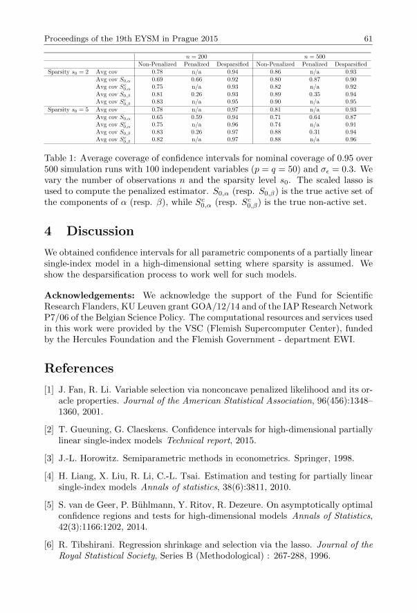
Proceedings of the 19th EYSM in Prague 2015 61
n = 200 n = 500Non-Penalized Penalized Desparsified Non-Penalized Penalized Desparsified
Sparsity s0 = 2 Avg cov 0.78 n/a 0.94 0.86 n/a 0.93Avg cov S0,α 0.69 0.66 0.92 0.80 0.87 0.90Avg cov Sc0,α 0.75 n/a 0.93 0.82 n/a 0.92Avg cov S0,β 0.81 0.26 0.93 0.89 0.35 0.94Avg cov Sc0,β 0.83 n/a 0.95 0.90 n/a 0.95
Sparsity s0 = 5 Avg cov 0.78 n/a 0.97 0.81 n/a 0.93Avg cov S0,α 0.65 0.59 0.94 0.71 0.64 0.87Avg cov Sc0,α 0.75 n/a 0.96 0.74 n/a 0.91Avg cov S0,β 0.83 0.26 0.97 0.88 0.31 0.94Avg cov Sc0,β 0.82 n/a 0.97 0.88 n/a 0.96
Table 1: Average coverage of confidence intervals for nominal coverage of 0.95 over500 simulation runs with 100 independent variables (p = q = 50) and σε = 0.3. Wevary the number of observations n and the sparsity level s0. The scaled lasso isused to compute the penalized estimator. S0,α (resp. S0,β) is the true active set ofthe components of α (resp. β), while Sc0,α (resp. Sc0,β) is the true non-active set.
4 Discussion
We obtained confidence intervals for all parametric components of a partially linearsingle-index model in a high-dimensional setting where sparsity is assumed. Weshow the desparsification process to work well for such models.
Acknowledgements: We acknowledge the support of the Fund for ScientificResearch Flanders, KU Leuven grant GOA/12/14 and of the IAP Research NetworkP7/06 of the Belgian Science Policy. The computational resources and services usedin this work were provided by the VSC (Flemish Supercomputer Center), fundedby the Hercules Foundation and the Flemish Government - department EWI.
References
[1] J. Fan, R. Li. Variable selection via nonconcave penalized likelihood and its or-acle properties. Journal of the American Statistical Association, 96(456):1348–1360, 2001.
[2] T. Gueuning, G. Claeskens. Confidence intervals for high-dimensional partiallylinear single-index models Technical report, 2015.
[3] J.-L. Horowitz. Semiparametric methods in econometrics. Springer, 1998.
[4] H. Liang, X. Liu, R. Li, C.-L. Tsai. Estimation and testing for partially linearsingle-index models Annals of statistics, 38(6):3811, 2010.
[5] S. van de Geer, P. Buhlmann, Y. Ritov, R. Dezeure. On asymptotically optimalconfidence regions and tests for high-dimensional models Annals of Statistics,42(3):1166:1202, 2014.
[6] R. Tibshirani. Regression shrinkage and selection via the lasso. Journal of theRoyal Statistical Society, Series B (Methodological) : 267-288, 1996.

Random Matrix Models with Heavy Tails
Johannes Heiny∗1 and Thomas Mikosch1
1University of Copenhagen, Denmark
Abstract: Many fields of modern sciences are faced with high-dimensional datasets. In order to explore the structure in the data the sample covariance matrix canbe used. Often dimension reduction techniques facilitate further analyzes of largedata matrices in genetic engineering and finance. Principal Component Analysisfor example makes a linear transformation of the data to obtain vectors of whichthe first few contain most of the variation in the data. These principal componentvectors correspond to the largest eigenvalues of the sample covariance matrix. Thismotivates to study the eigenvalue decomposition of the sample covariance matrix.
Random Matrix Theory is concerned with the spectral properties of large di-mensional random matrices. In this context both the distribution of the entriesof a random matrix as well as their dependence structure play a crucial role. Thecase of heavy-tailed components is of particular interest and the theory is not aswell developed as in the light-tailed case.
We consider the (random) sample covariance matrix of a multivariate timeseries. The p-dimensional time series constitutes a linear process across time andbetween components. The input noise of the linear process is assumed to havea regularly varying tail with index α ∈ (0, 4). For such distributions momentshigher than α cease to exist. If we have n observations from this time series, wecan calculate the corresponding sample covariance matrix. In classical multivariatestatistics p is fixed and relatively small in comparison to the sample size n. In oursetting both the dimension and the sample size tend to infinity simultaneously.
If the multivariate time series is iid across time and between the components,Auffinger et al. [1] showed that the point process of properly normalized eigenvaluesof the sample covariance matrix converges in distribution to a Poisson point processthat only depends on the index of regular variation. Davis et al. [2] provided anextension by dropping the independence assumption across time. We also drop theindependence between components. In particular, we study the asymptotic behav-ior of the largest eigenvalues of such a sample covariance matrix by approximationresults.
Keywords: regular variation, sample covariance matrix, largest eigenvalues, de-pendent entries
AMS subject classifications: 60B20, 60F05, 60F10, 60G10, 60G70
Acknowledgements: Johannes Heiny’s research is supported by the Danish Re-search Council Grant DFF-4002-00435 “Large random matrices with heavy tailsand dependence”.
∗Corresponding author: [email protected]

Proceedings of the 19th EYSM in Prague 2015 63
References
[1] Auffinger, A., Ben Arous, G. and Peche, S. (2009) Poisson convergence for thelargest eigenvalues of heavy tailed random matrices. Ann. Inst. H. Poincare,Probab. Statist. 45, 589–610.
[2] Davis, R.A., Pfaffel, O. and Stelzer, R. (2014) Limit theory for the largesteigenvalues of sample covariance matrices with heavy tails. Stoch. Proc. Appl.124, 18–50.

Comparison of Methods for Variable Selection inHigh-Dimensional Linear Mixed Models
Jozef Jakubık∗
Institute of Measurement Science, Slovak Academy of Sciences, Bratislava,Slovakia
Abstract: Currently is the analysis of high-dimensional data a popular field ofresearch, thanks to many applications e.g. in genetics. At the same time, the typeof problems that tend to arise in genetics, can often be modelled using LMMs inconjunction with high-dimensional data. In this paper we introduce two new meth-ods and briefly compare them to existing methods, which can be used for variableselection in high-dimensional linear mixed models. We compare the methods on“small dimension” high-dimensional data, because some of the compared methodsare not suitable for very high dimensions. As we will show in a simulation study,both methods perform well compared to existing methods.
Keywords: linear mixed model, variable selection, high-dimensional data
AMS subject classifications: 62J07
1 Introduction
The linear mixed model (LMM) allows us to specify the covariance structure of themodel, which enables us to capture relationships in data, for example populationstructure, family relatedness etc. Therefore, LMMs are often preferred to linearregression models. Consider a LMM of the form
Y = Xβ +Zu+ ε,
where
Y is n× 1 vector of observations,
X is n× p matrix of regressors,
β is p× 1 vector of unknown fixed effects,
Z is n× q matrix of predictors,
u is q × 1 vector of random effects with the distribution N (0,D),
ε is n×1 error vector with the distribution N (0,R = σ2I) and independentfrom u.
∗Corresponding author: [email protected]

Proceedings of the 19th EYSM in Prague 2015 65
In genome-wide association studies in genetics, one studies the dependence ofphenotype on the genotype. Genetic information can consist of up to 106 variables,but only information about the genotype of a small group of subjects is available.Variable selection in high-dimensional data refers to the selection of a small groupof variables (denote it S0, and s0 = |S0| the number of relevant variables) whichinfluence observations. In our case we assume, that matrix X is high-dimensionaland we select only variables from matrix X.
More information about the model can be found in section 3.
2 Methods
In this paper we compare five methods for variable selection in high-dimensionalLMMs.
All of the mentioned methods are primarily β estimation methods, not selectionmethods. However they can be thought of as selection methods if we define selectedvariables to be those for which βi 6= 0 for i = 1, . . . , p.
2.1 LASSO
Least absolute shrinkage and selection operator [4, 1] is an established methodfor selecting variables in linear regression models. LASSO corresponds to the `1-penalized ordinary least squares estimate:
β = arg minβ
[‖Y −Xβ‖22 + λ‖β‖1
],
where λ is a fixed penalized parameter.In this study we use the LASSO as the reference, as it ignores LMM data
structure. For the LASSO method we use the built-in MATLAB function lasso().
2.2 LMMLASSO
Authors in [3] suggest a method based on the minimization of the non-convexobjective function consisting of the `1 penalized maximum likelihood estimate ofparameter β from Y ∼ N (Xβ,V (= ZDZT +R)):
(β, D, R) = arg minβ,D,R
[1
2log |V |+ 1
2(Y −Xβ)TV −1(Y −Xβ) + λ‖β‖1
],
where λ is a fixed parameter. For this method we used the language R packagelmmlasso, which uses the coordinate gradient descent algorithm to the optimizeobjective function.
2.3 LASSOP
In paper [2] authors introduce a method based on the log-likelihood of the complexdata (Y T,uT)T penalized with the `1 penalization:

66 Jakubık -- Methods for Variable Selection in High-Dimensional LMM
(β, D, R) = arg minβ,D,R
[log |R|+ (Y −Xβ −Zu)TR−1(Y −Xβ −Zu)
+ log |D|+ uTD−1u+ λ‖β‖1],
where λ is a fixed parameter. The objective function is non-convex, like inLMMLASSO. This method is implemented in language R in package MMS. Theoptimize problem in this implementation is solved by the adjusted EM algorithm.
2.4 New approach one
The first approach consists in a transformation that removes group effects fromdata. The principle of this transformation is widely used in data analysis, for ex-ample in restricted/residual maximum likelihood (REML). In our case we transformthe data as follows
X = (I −ZZ+)X,
Y = (I −ZZ+)Y ,
where Z+ is the pseudoinverse matrix. The transformation eliminates randomsegments of the problem (associated with matrix Z), which allows us to use theLASSO method for linear regression model.
2.5 New approach two
Methods LMMLASSO and LASSOP are based on non-convex optimization prob-lems with one penalty parameter. For problems of dimension higher than 104
are methods based on non-convex optimization problems almost unusable, becausetheir computational complexity is beyond the capabilities of current computers.One of the possible solutions to this problem is the simplification of the optimizedfunction to a convex function. Therefore, we have proposed a method based on thesolution to the following convex problem
(β, u) = arg minβ,u
‖Y −Xβ −Zu‖22 − λ‖β‖1 − Λ
q∗∑i=1
‖ iu‖22
,where λ and Λ are fixed parameters, q∗ is the number of variance components
(without error) and iu is the part of vector u belonging to the i-th variance com-ponent.
Basically we are exchanging computational complexity for the need to inspecta two-dimensional parameter space. We implement the method in MATLAB usingthe modeling system CVX and the solver Mosek.

Proceedings of the 19th EYSM in Prague 2015 67
3 Simulation study
This study compares the presented methods on high-dimensional data with “smalldimension”, because the curent implementations of methods LMMLASSO andLASSOP are commonly unable to solve problems of dimension higher then p = 103.
Data in our simulation study are divided into twenty groups of six observations.Together we have n = 120 observations. For each observation we observe p = 150variables, but only s0 = 1, . . . , 10 variables influence the observations. Relevantvariables are randomly selected from all variables and the effect of relevant variablesis one. The effect of other variables is zero. Matrix Z captures group structureof the data. For every group we observe two variables, therefore we consider twovariance components and the error variance component. Z is a block diagonalmatrix and u consist of two parts, each for one variance component. Both parts ofthe random effects u are randomly selected from N (0,D = 2 · I). Errors are fromN (0, I).
For all mentioned methods we get different sets of selected variables for differentparameters λ or Λ. We generate a hundred problems as described in the previousparagraph. As a correctly solved problem we consider only a problem for which themethod gives for at least one parameter or parameter combination as the selectedvariable set exactly set S0. Figure 1 shows the number of correctly solved problemsfor all five methods for different numbers of relevant variables (from 1 to 10).
s02 4 6 8 10
Cor
rect
ly s
olve
d pr
oble
ms
0
20
40
60
80
100
LASSOLMMLASSOLASSOPNew approach oneNew approach two
Figure 1: Comparison of the number of correctly solved problems for different s0
with five different methods.

68 Jakubık -- Methods for Variable Selection in High-Dimensional LMM
4 Conclusion
In Figure 1 we can see that for small numbers of relevant variables all methods arealmost infallible. With the increasing number of relevant variables, the accuracy ofmethods decreases. This is understandable, because with more relevant variablesthe correlation of each relevant variable with the vector of observations decreases.Therefore, it is more difficult to identify correctly the exact set of variables. Theaccuracy of methods LMMLASSO and LASSOP decreases faster. The seeminglyweak performance of these methods is caused by the very strict condition of correct-ness. Often, the sets of selected variables identify by these methods contained onlya few unnecessary variables. This may be due to the implementation in differentlanguages.
This study hints at the potential of the newly proposed methods to significantlyoutperform both the LMMLASSO and the LASSOP. The newly proposed methodsare also suitable for high-dimensional data with dimension up to 105.
However, this is only a preliminary study and one of the first addressing thequestion. A more extensive analysis can be expected in the future.
Acknowledgements: The work was supported by the Scientific Grant AgencyVEGA of the Ministry of Education of the Slovak Republic and the Slovak Academyof Sciences, by the projects VEGA 2/0047/15 and VEGA 2/0043/13.
References
[1] P. Buhlmann and S. Van De Geer. Statistics for high-dimensional data: meth-ods, theory and applications. Springer Science & Business Media, 2011.
[2] F. Rohart, M. San Cristobal, and B. Laurent. Selection of fixed effects in highdimensional linear mixed models using a multicycle ECM algorithm. Compu-tational Statistics & Data Analysis, 80:209–222, Dec. 2014.
[3] J. Schelldorfer, P. Buhlmann, and S. van De Geer. Estimation for High-Dimensional Linear Mixed-Effects Models Using `1-Penalization. ScandinavianJournal of Statistics, 38(2):197–214, June 2011.
[4] R. Tibshirani. Regression shrinkage and selection via the lasso. Journal of theRoyal Statistical Society. Series B (Methodological), 58:267–288, 1996.

Confidence Regions for High-Dimensional SparseModels
Jana Jankova∗1 and Sara van de Geer1
1ETH Zurich, Switzerland
Abstract: In many important statistical applications the number of parametersmay be much larger than the sample size. One of the main approaches to deal withthis situation is to assume that the underlying true model is sparse so that only asufficiently small number of parameters are important. Methods for point estima-tion in such sparse high-dimensional settings have been extensively studied in thepast years (see [1]). Less work has yet been done on developing methodology forinference for the parameters of interest in this setting. We propose an estimator forlow-dimensional parameters of the high-dimensional vector and show it is asymp-totically normal and regular, leading to confidence regions for low-dimensionalparameters. Our approach is based on `1-penalized M-estimators which serve asinitial estimates for construction a one-step corrected estimator. We show validityof the suggested approach in several situations including quantile regression wherethe loss function is not differentiable or precision matrix estimation [2], and fur-ther consider general high-dimensional models. Under a sparsity assumption onthe high-dimensional parameter, smoothness conditions on the expected loss andan entropy condition we show that the proposed de-sparsified estimator is asymp-totically normal. This leads to uniformly valid confidence regions and hypothesistesting for low-dimensional parameters.
Keywords: high-dimensional models, sparsity, inference, lasso
AMS subject classifications: 62F12
References
[1] Buhlmann, P. and van de Geer, S. Statistics for high-dimensional data. Springer(2011).
[2] Jankova, J. and van de Geer, S. Confidence intervals for high-dimensionalinverse covariance estimation. ArXiv :1403.6752 (2014).
[3] van de Geer, S., Buhlmann, P., Ritov, Y., and Dezeure, R. On asymptoticallyoptimal confidence regions and tests for high-dimensional models. Annals ofStatistics, 42(3) (2014), 1166-1202.
[4] Zhang, C.-H. and Zhang, S. S. Confidence intervals for low-dimensional pa-rameters in high-dimensional linear models. Journal of the Royal StatisticalSociety: Series B, 76 (2014), 217–242.
∗Corresponding author: [email protected]

Asymptotic Theory forCopula Rank-Based Periodograms
Tobias Kley∗
Ruhr-Universitat Bochum, Fakultat fur Mathematik, Germany
Abstract: Alternative spectral concepts for the analysis of time series recentlyhave been considered by various authors. The copula spectral density kernels intro-duced in [3] provide a full characterization of the copulas associated with the pairs(Xt, Xt−k) in a process (Xt)t∈Z, and account for important dynamic features, suchas changes in the conditional shape (skewness, kurtosis), time-irreversibility, or de-pendence in the extremes, that their traditional counterparts cannot capture. De-spite various proposals for estimation strategies, only quite incomplete asymptoticdistributional results are available so far for the proposed estimators, which con-stitutes an important obstacle for their practical application. This paper containsmotivation and definitions for the class of smoothed rank-based cross-periodogramsconsidered in [13]. An asymptotic analysis is presented: for a very general class of(possibly non-linear) processes, properly scaled and centered smoothed versions ofthose cross-periodograms, indexed by couples of quantile levels, converge weakly,as stochastic processes, to Gaussian processes. Note that the present paper is avery condensed version of [13], where technical details and simulation results canbe found.
Keywords: time series, spectral analysis, quantiles, copulas, ranks
AMS subject classifications: 62M15, 62G35
1 Introduction
Frequency domain methods play a central role in the nonparametric analysis of timeseries. The classical approach is based on the spectral density which is traditionallydefined as the Fourier transform of the autocovariance function of the process understudy. Common tools for the estimation of spectral densities are the periodogramand its smoothed versions. The success of periodograms in time series analysis isrooted in their fast and simple computation (through the fast Fourier transformalgorithm) and their interpretation in terms of cyclic behavior, both of a stochasticand of deterministic nature, which in specific applications are more illuminatingthan time-domain representations.
Being intrinsically connected to means and covariances, the traditional spectralanalysis inherits both the nice features (such as optimality properties in the analysisof Gaussian series) of L2-methods, but also their weaknesses: they are lackingrobustness against outliers and heavy tails, and are unable to capture important
∗Corresponding author: [email protected]

Proceedings of the 19th EYSM in Prague 2015 71
dynamic features such as changes in the conditional shape (skewness, kurtosis),time-irreversibility, or dependence in the extremes.
Various extensions and modifications of the traditional periodogram were pro-posed to remedy those drawbacks (see for example [6], [9], [10], [14], Chapter 8of [20], and [21]). While the objective of those attempts is a robustification ofclassical tools, they essentially aim at protecting existing spectral methods againstthe impact of possible outliers or violations of distributional assumptions.
Recently, alternative spectral concepts that account for more general dynamicfeatures were proposed. A first step in that direction was taken by [7], who proposesa generalized spectral density with covariances replaced by joint characteristic func-tions. In the specific problem of testing pairwise independence, [8] introduces a teststatistic based on the Fourier transforms of (empirical) joint distribution functionsand copulas at different lags. The strand of literature indicating the renewed surgeof interest in that type of concept includes [2], [3], [5], [15], [16], [17], and [18]. Amore detailed account of these and some further contributions are given in [13].
The objective of the present paper is to provide a short, comprehensive pre-sentation of the general class of smoothed rank-based copula cross-periodogramsdiscussed at length in [13]. Their asymptotic properties are discussed in Section 3.For a detailed discussion, applications and a simulation study the reader shall bereferred to the full version of the paper (i. e. [13]).
2 Copula spectral density kernels and rank-basedcopula periodograms
Let (Xt)t∈Z denote a strictly stationary, real-valued process, of which we observe afinite stretch X0, ..., Xn−1. Denote by F the marginal distribution function of Xt,and by qτ := infx ∈ R : τ ≤ F (x), τ ∈ [0, 1] the corresponding quantile function,where we use the convention inf ∅ = ∞. Note that if τ ∈ 0, 1 then −∞ and ∞are possible values for qτ . Our main object of interest is the copula spectral densitykernel
fqτ1 ,qτ2 (ω) :=1
2π
∑k∈Z
e−iωkγUk (τ1, τ2), ω ∈ R, (τ1, τ2) ∈ [0, 1]2, (1)
based on the copula cross-covariances
γUk (τ1, τ2) := Cov(IF (Xt) ≤ τ1, IF (Xt−k) ≤ τ2
), k ∈ Z.
Note that fqτ1 ,qτ2 (ω) exists under mild mixing assumptions. These quantities wereintroduced in [3], and generalize the τ -th quantile spectral densities of [5], withwhich they coincide for τ1 = τ2 = τ ; an integrated version actually was firstconsidered by [8].
It can be shown (cf. [3]) that the copula spectral densities provide a completedescription of the pairwise copulas of a time series. Thus, by accounting for muchmore than the covariance structure of a series, it extends and supplements theclassical L2-spectral density.

72 Kley -- Asymptotic Theory for Copula Rank-Based Periodograms
It is important to observe that γUk (τ1, τ2) and fqτ1 ,qτ2 (ω) can be seen as thecross-covariance and cross-spectrum of the bivariate process(
IF (Xt) ≤ τ1, IF (Xt) ≤ τ2). (2)
Thus, an estimator for the cross spectrum of (2) is also an estimator for fqτ1 ,qτ2 (ω).If F were known and (Xt)t∈Z was observed, we could determine (2) and followthe lines of [1] to construct an estimator. Observe, that (2) has binary-valuedcomponent processes, such that classical assumptions regarding the dependencystructure (e. g. linearity of the process) can fail to hold. The estimation of crossspectra of general non-linear processes has been and remains to be an active domainof research (see [1] for early results, and [4], [19] or [22] for more recent references).
To handle the case where F is unknown, it is reasonable to estimate the un-known F with the empirical distribution function Fn(x) := n−1
∑n−1t=0 IXt ≤ x.
More precisely, we define In,R as the collection
Iτ1,τ2n,R (ω) :=1
2πndτ1n,R(ω)dτ2n,R(−ω), dτn,R(ω) :=
n−1∑t=0
IFn(Xt) ≤ τe−iωt, (3)
ω ∈ R, (τ1, τ2) ∈ [0, 1]2, τ ∈ [0, 1]. Note that nFn(Xt) is the rank of Xt amongX0, . . . , Xn−1. Hence, we will refer to In,R as the rank-based copula periodogram;shortly, the CR-periodogram. Let denote the Hoffman–Jørgensen convergence,namely, the weak convergence in the space of bounded functions [0, 1]2 → C, whichwe denote by `∞C ([0, 1]2). Note that results in empirical process theory are typicallystated for spaces of real-valued, bounded functions; see Chapter 1 of [23]. Byidentifying `∞C ([0, 1]2) with the product space `∞([0, 1]2)× `∞([0, 1]2) these resultstransfer immediately. We will see (Theorem 13) that, under suitable assumptions,(
Iτ1,τ2n,R (ω))
(τ1,τ2)∈[0,1]2 (I(τ1, τ2;ω)
)(τ1,τ2)∈[0,1]2
as n→∞,
for any fixed frequencies ω 6= 0 mod 2π, where the limit I is such that
E[I(τ1, τ2;ω)] = fqτ1 ,qτ2 (ω) for all (τ1, τ2) ∈ [0, 1]2 and ω 6= 0 mod 2π
and I(·, ·;ω1) and I(·, ·;ω2) are independent as soon as both ω1 − ω2 6= 0 mod 2πand ω1 + ω2 6= 0 mod 2π. In view of this asymptotic independence at differentfrequencies, it seems natural to consider smoothed versions of Iτ1,τ2n,R (ω), namely,
for (τ1, τ2) ∈ [0, 1]2 and ω ∈ R, averages of the form
Gn,R(τ1, τ2;ω) :=2π
n
n−1∑s=1
Wn
(ω − 2πs/n
)Iτ1,τ2n,R (2πs/n), (4)
where Wn denotes a sequence of weighting functions.
3 Asymptotic properties
We make the following assumption regarding the process (Xt)t∈Z:

Proceedings of the 19th EYSM in Prague 2015 73
(A) Assume that the process (Xt)t∈Z is strictly stationary and exponentiallyα-mixing, i. e., there exists constants K <∞ and κ ∈ (0, 1), such that,
α(n) := supA∈σ(X0,X−1,...)B∈σ(Xn,Xn+1,...)
|P(A ∩B)− P(A)P(B)| ≤ Kκn , n ∈ N. (5)
Theorem 13. Assume that F is continuous and that (Xt)t∈Z satisfies Assump-tion (A). Then, for every fixed ω 6= 0 mod 2π,(
Iτ1,τ2n,R (ω))
(τ1,τ2)∈[0,1]2 (I(τ1, τ2;ω)
)(τ1,τ2)∈[0,1]2
in `∞C ([0, 1]2).
The (complex-valued) limiting processes I, are of the form
I(τ1, τ2;ω) =1
2πD(τ1;ω)D(τ2;ω), (τ1, τ2) ∈ [0, 1]2,
with D(τ ;ω) = C(τ ;ω) + iS(τ ;ω) where C and S denote two centered jointly Gaus-sian processes. For ω ∈ R, their covariance structure takes the form
E[(C(τ1;ω),S(τ1;ω))′(C(τ2;ω),S(τ2;ω)))
]= π
(<fqτ1 ,qτ2 (ω) −=fqτ1 ,qτ2 (ω)=fqτ1 ,qτ2 (ω) <fqτ1 ,qτ2 (ω)
).
Moreover, D(τ ;ω) = D(τ ;ω + 2π) = D(τ ;−ω), and the family D(·;ω) : ω ∈ [0, π]is a collection of independent processes.
In order to establish the convergence of the smoothed CR-periodogram pro-cess (4), we require the weights Wn in (4) to satisfy the following assumption:
(W) The weight function W is real-valued and even, with support [−π, π]; more-over, it has bounded variation, and satisfies
∫ π−πW (u)du = 1.
Denoting by bn > 0, n = 1, 2, . . ., a sequence of scaling parameters suchthat bn → 0 and nbn →∞ as n→∞, define
Wn(u) :=
∞∑j=−∞
b−1n W (b−1
n [u+ 2πj]).
Theorem 14. Let Assumptions (A) and (W) hold. Assume that X0 has a contin-uous distribution function F and that there exist constants κ > 0, k ∈ N, s. t.
bn = o(n−1/(2k+1)) and bnn1−κ →∞.
Then, for any fixed ω ∈ R, the process√nbn
(Gn,R(τ1, τ2;ω)− fqτ1 ,qτ2 (ω)−B(k)
n (τ1, τ2;ω))τ1,τ2∈[0,1]
H(·, ·;ω) (6)
in `∞C ([0, 1]2), where the bias B(k)n is given by
B(k)n (τ1, τ2;ω) :=
k∑j=2
bjnj!
∫ π
−πvjW (v)dv
dj
dωjfqτ1 ,qτ2 (ω) ω 6= 0 mod 2π,
n(2π)−1τ1τ2 ω = 0 mod 2π.
(7)
74 Kley -- Asymptotic Theory for Copula Rank-Based Periodograms
The process H(·, ·;ω) in (6) is a centered Gaussian process characterized by
Cov(H(u1, v1;ω
), H(u2, v2;ω)) = 2π
(∫ π
−πW 2(w)dw
)×(fqu1 ,qu2 (ω)fqv2 ,qv1 (ω) + fqu1 ,qv2 (ω)fqv1 ,qu2 (ω)Iω = 0 mod π
).
Moreover, H(ω) = H(ω + 2π) = H(−ω), and the family H(ω), ω ∈ [0, π] is acollection of independent processes. In particular, the weak convergence (6) holdsjointly for any finite fixed collection of frequencies ω.
Theorem 14 can be used to conduct asymptotic inference in various ways. Animportant example is the construction of asymptotic confidence intervals (see Re-mark 3.4 and Section 5 in [13] for details). An R package is available (see [11, 12]).
Acknowledgements: This work has been supported by the Sonderforschungs-bereich “Statistical modelling of nonlinear dynamic processes” (SFB 823) of theDeutsche Forschungsgemeinschaft. The author was supported by a PhD Grant ofthe Ruhr-Universitat Bochum and by the Ruhr-Universitat Research School fundedby Germany’s Excellence Initiative [DFG GSC 98/1]. This short note is a summary,essentially, of results obtained in collaboration with Holger Dette, Marc Hallin, andStanislav Volgushev, whom I thank very much.
References
[1] D. R. Brillinger. Time Series: Data Analysis and Theory. Holt, Rinehart andWinston, Inc., New York, 1975.
[2] R. A. Davis, T. Mikosch, and Y. Zhao. Measures of serial extremal dependenceand their estimation. Stoch. Proc. Appl., 123:2575–2602, 2013.
[3] H. Dette, M. Hallin, T. Kley, and S. Volgushev. Of copulas, quantiles, ranks andspectra: An L1-approach to spectral analysis. Bernoulli, forthcoming, 2015+.
[4] L. Giraitis and H. L. Koul. On asymptotic distributions of weighted sums ofperiodograms. Bernoulli, 19(5B):2389–2413, 2013.
[5] A. Hagemann. Robust spectral analysis (arxiv:1111.1965v2). ArXiv, 2013.
[6] J. B. Hill and A. McCloskey. Heavy tail robust frequency domain estima-tion. Available online: http://www.econ.brown.edu/fac/adam_mccloskey/
Research_files/FDTTQML.pdf, 2013.
[7] Y. Hong. Hypothesis testing in time series via the empirical characteris-tic function: a generalized spectral density approach. J. Am. Stat. Assoc.,94(448):1201–1220, 1999.
[8] Y. Hong. Generalized spectral tests for serial dependence. J. Roy. Stat. Soc.B, 62(3):557–574, 2000.

Proceedings of the 19th EYSM in Prague 2015 75
[9] V. Katkovnik. Robust M-periodogram. IEEE T. Signal Proces., 46(11):3104–3109, 1998.
[10] R. Kleiner, R. D. Martin, and D. J. Thomson. Robust estimation of powerspectra. J. Roy. Stat. Soc. B, 41(3):313–351, 1979.
[11] T. Kley. Quantile-based spectral analysis in an object-oriented frameworkand a reference implementation in R: The quantspec package. J. Stat. Softw.,forthcoming, 2015+.
[12] T. Kley. quantspec: Quantile-based spectral analysis functions, 2015. R packageversion 1.0-3.
[13] T. Kley, S. Volgushev, H. Dette, and M. Hallin. Quantile Spectral Processes:Asymptotic Analysis and Inference. Bernoulli, forthcoming, 2015+.
[14] C. Kluppelberg and T. Mikosch. Some limit theory for the self-normalisedperiodogram of stable processes. Scand. J. Stat., 21:485–491, 1994.
[15] J. Lee and S. S. Rao. The quantile spectral density and comparison basedtests for nonlinear time series (arxiv:1112.2759v2). ArXiv, 2012.
[16] T.-H. Li. Laplace periodogram for time series analysis. J. Am. Stat. Assoc.,103(482):757–768, 2008.
[17] T.-H. Li. Quantile periodograms. J. Am. Stat. Assoc., 107(498):765–776, 2012.
[18] T.-H. Li. Time Series with Mixed Spectra: Theory and Methods. CRC Press,Boca Raton, 2013.
[19] W. Liu and W. B. Wu. Asymptotics of spectral density estimates. EconometricTheory, 26(4):1218–1245, 2010.
[20] R. Maronna, D. Martin, and V. Yohai. Robust Statistics: Theory and Methods.Wiley Series in Probability and Statistics. Wiley, 2006.
[21] T. Mikosch. Periodogram estimates from heavy-tailed data. In R. A. Adler,R. Feldman, and M. S. Taqqu, editors, A Practical Guide to Heavy Tails: Sta-tistical Techniques for Analysing Heavy-Tailed Distributions, pages 241–258.Birkhauser, Boston, 1998.
[22] X. Shao and W. B. Wu. Asymptotic spectral theory for nonlinear time series.Ann. Stat., 35(4):1773–1801, 2007.
[23] A. van der Vaart and J. Wellner. Weak Convergence and Empirical Processes:With Applications to Statistics. Springer, New York, 1996.
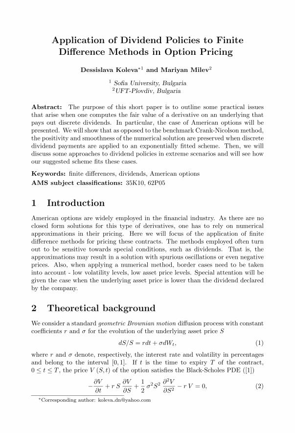
Application of Dividend Policies to FiniteDifference Methods in Option Pricing
Dessislava Koleva∗1 and Mariyan Milev2
1 Sofia University, Bulgaria2UFT-Plovdiv, Bulgaria
Abstract: The purpose of this short paper is to outline some practical issuesthat arise when one computes the fair value of a derivative on an underlying thatpays out discrete dividends. In particular, the case of American options will bepresented. We will show that as opposed to the benchmark Crank-Nicolson method,the positivity and smoothness of the numerical solution are preserved when discretedividend payments are applied to an exponentially fitted scheme. Then, we willdiscuss some approaches to dividend policies in extreme scenarios and will see howour suggested scheme fits these cases.
Keywords: finite differences, dividends, American options
AMS subject classifications: 35K10, 62P05
1 Introduction
American options are widely employed in the financial industry. As there are noclosed form solutions for this type of derivatives, one has to rely on numericalapproximations in their pricing. Here we will focus of the application of finitedifference methods for pricing these contracts. The methods employed often turnout to be sensitive towards special conditions, such as dividends. That is, theapproximations may result in a solution with spurious oscillations or even negativeprices. Also, when applying a numerical method, border cases need to be takeninto account - low volatility levels, low asset price levels. Special attention will begiven the case when the underlying asset price is lower than the dividend declaredby the company.
2 Theoretical background
We consider a standard geometric Brownian motion diffusion process with constantcoefficients r and σ for the evolution of the underlying asset price S
dS/S = rdt+ σdWt, (1)
where r and σ denote, respectively, the interest rate and volatility in percentagesand belong to the interval [0, 1]. If t is the time to expiry T of the contract,0 ≤ t ≤ T , the price V (S, t) of the option satisfies the Black-Scholes PDE ([1])
−∂V∂t
+ r S∂V
∂S+
1
2σ2S2 ∂
2V
∂S2− r V = 0, (2)
∗Corresponding author: koleva [email protected]

Proceedings of the 19th EYSM in Prague 2015 77
endowed by its initial and boundary conditions. The solution V (S, t) depends onthe two independent variables S and t. It should be noted that the option pricecan move on the positive real axis interval [0,+∞).
Finite difference schemes aim in approximating the solution of a PDE by solvinga set of discretized equations. A discussion on different methods can be found in[7]. The most famous schemes are the explicit, implicit and Crank-Nicolson. Theyall rely on taking central differences when discretizing the partial derivatives withrespect to the underlying asset S, i.e.
∂V
∂S=Vi,j+1 − Vi,j−1
2h,
∂2V
∂S2=Vi,j+1 + Vi,j−1 − 2Vi,j
h2. (3)
Here, Vi,j denotes the value of the option at i-th point in time and j-th pointin the discretized interval [0, Smax]. The time step has a size of k and the assetstep has a size of h.
The explicit scheme then takes the time derivative as forward difference of t(backward in physical time)
∂V
∂t=Vi,j − Vi−1,j
k. (4)
It is accurate at order O(k, h). However, it is stable and convergent only for
λ =k
h2≤ 0.5. (5)
That is, problems may occur for small time steps.The implicit scheme takes the time derivative as backward difference of t (for-
ward in physical time)∂V
∂t=Vi+1,j − Vi,j
k. (6)
It is accurate at order O(k, h). Also, the implicit finite difference scheme is uncon-ditionally stable.
The Crank-Nicolson scheme is the average of the explicit and implicit. It isaccurate at order O(k2, h2). As the implicit method, Crank-Nicolson is uncondi-tionally stable. However, in the presence of points of discountinuity in the initialconditions or with special boundary values, small asset steps may introduce spuri-ous ocsillations. The latter may even lead to obtaining negative option prices. Adiscussion on these effects can be found in [4], for example.
The scheme introduced by [3] is an interesting alternative to the previouslydescribed methods. It is exponentially fitted, based on a hyberbolic cotangentfunction. Consider the operator L defined as:
LV = −∂V∂t
+ µ(S, t)∂V
∂S+ σ(S, t)
∂2V
∂S2+ b(S, t)V, (7)
where µ(S, t) = rS, σ(S, t) = 12σ
2S2 and b(S, t) = −r.Replacing the derivatives, the fitted operator is defined by
LhkUnj = −
Un+1j − Unj
k+ µn+1
j
Un+1j+1 − Un+1
j−1
2h+ ρn+1
j
δ2xU
n+1j
h2+ bn+1
j Un+1j , (8)

78 Koleva and Milev -- Dividends for Finite Difference Methods in Option Pricing
S41 42 43 44 45 46 47 48 49
Opt
ion
Val
ue (
V)
0
0.5
1
1.5
2Crank-Nicolson for American Put Option with One Dividend
cn
Figure 1: Crank-Nicolson scheme for an American put option.
where h and k are the space and time step, respectively. The factor ρ is defined as
ρn+1j =
µn+1j h
2coth
µn+1j h
2σn+1j
. (9)
The scheme is stable and consistent. Moreover, it converges regardless of thevolatility size. It does not suffer from oscillations for extreme parameter values andbehaves good for special conditions (such as barriers) and low volatility environ-ment ([6]). The method is of order O(k, h).
In what follows we apply dividends to the Duffy scheme and explore its com-patibility with a few dividend policies.
3 Results
With an implementation based on [2], the discrete dividend extension was appliedto the scheme suggested by Duffy. It handles low volatility levels and provides asmooth and oscillation-free solution when pricing American options. An exampleis run on an American put option with current underlying value of 40, strike =40, rate = 0.1, volatility = 0.05, time to maturity of one year, and an expecteddividend of size 5 in 0.6 years from evaluation date.
Figure 1 plots the result obtained by the Crank-Nicolson finite difference scheme.As one can easily see, the price function suffers from spurious oscillations. Then,on Figure 2 is provided the outcome of employing the Duffy scheme on the verysame option. The undesired price fluctuations are gone and the result is a smoothfunction.
4 Discussion on Dividend Policies
When pricing derivatives on an underlying asset which pays out dividends, onehas to deal with the shifts these payments cause to the underlying price. A broadreview of different dividend policies can be found in [5]. Here we discuss some ofthem and show how the Duffy scheme fits into these policies.
Since the classical Black-Scholes option pricing model has become popular, prac-titioners and academics are suggesting various approaches to applying dividends to

Proceedings of the 19th EYSM in Prague 2015 79
S41 42 43 44 45 46 47 48 49
Opt
ion
Val
ue (
V)
0
0.5
1
1.5
2Duffy for American Put Option with One Dividend
Duffy
Figure 2: Duffy scheme for an American put option
the underlying asset price. The continuous dividends assumption is oversimplify-ing as longer term dividends are less predictable. Another simple model suggestsupdating the stock series with the discounted expected dividend which again shiftsthe price inaccurately for dividends far in the future. A separate group of policiesis based on applying an adjustment to the volatility term. An approach which isinefficient in terms of computational time is employing non-recombining binomialtrees.
It is interesting to review the policies suggested in case of a serious drop in theunderlying value. That is, what should the numerical approach be if the asset pricebecomes lower than the declared dividend? If S denotes the underlying price atthe time the dividend should be paid out and D is the declared dividend size, inthe scenario just described we have that S < D. The two suggested policies forthis case are survivor and liquidator.
According to the survivor policy, the company will pay no dividend to its share-holders. In other words, the company will have no ability to fulfill the declaredpayment but will still survive.
On the other hand, the liquidator policy adopts a more strict view. If thecompany finds itself in a situation when its share market price is lower than thedeclared dividend, it should pay out an amount equal to the current asset price.This is the policy encorporated in the Duffy scheme.
Despite having a marginal effect, the choice of a dividend policy in case of asevere drop in asset prices is a step towards having a fully specified model.
5 Conclusion
This short paper presented a brief outline of some of the most popular finite dif-ference methods employed in option pricing, together with the main problems intheir application. Then it was shown that the Duffy scheme is suitable for ap-plying discrete dividends, as it does not suffer from numerical issues that mayresult in spurious oscillations. Finally, different dividend policies in option pricingapproximations were discussed.

80 Koleva and Milev -- Dividends for Finite Difference Methods in Option Pricing
References
[1] F. Black and M. Scholes. The pricing of options and corporate liabilities. Jour-nal of Political Economy, (81):637–654, 1973.
[2] P. Brandimarte. Numerical Methods in Finance: a MATLAB - based Introduc-tion. John Wiley & Sons, New York, 2001.
[3] D. Duffy. A critique of the Crank-Nicolson scheme, strengths and weaknessesfor financial instrument pricing. Wilmott Magazine, pages 68–74, July 2004.
[4] D. Duffy. Finite difference methods in financial engineering: A partial differ-ential equation approach. John Wiley & Sons, Chichester, 2006.
[5] E. Haug, J. Haug, and A. Lewis. Back to basics: A new approach to the discretedividend problem. Wilmott Magazine, pages 37–47, September 2003.
[6] M. Milev and A. Tagliani. Low volatility options and numerical diffusion offinite difference schemes. Serdica Mathematical Journal, 36(3):223–236, 2010.
[7] P. Wilmott. Derivatives: The theory and practice of financial engineering. JohnWiley & Sons, Chichester, University edition, 1998.

Estimation of the Offspring Mean Matrix in2-Type Critical Galton-Watson Processes
Kristof Kormendi∗1 and Gyula Pap2
1MTA-SZTE Analysis and Stochastics Research Group, University of Szeged,Aradi vertanuk tere 1, H–6720 Szeged, Hungary.
2 Bolyai Institute, University of Szeged, Aradi vertanuk tere 1, H–6720 Szeged,Hungary.
Abstract: The well known Galton–Watson process can be generalized the fol-lowing way; suppose the population consists of multiple types of individuals andallow the offsprings to have a different type than their parents. Denote the numberof types by d. To describe this process we have to assign a d-dimensional offspringdistribution to each of the types. The offspring mean matrix is a matrix whosecolumns consist of the expectation of these distributions.
In the single-type case we distinguish between subcritical, critical and super-critical processes based on the relation of the offspring mean to 1. For multi-typeGalton–Watson processes we make the same distinction based on the spectral ra-dius of the offspring mean matrix. Immigration can be introduced to the modelexactly as in the single-type case, by adding i.i.d. random vectors representing thenumber of immigrants in each generation.
In Ispany et al. [1] we describe the asymptotic properties of the conditionalleast squares estimate of the offspring mean matrix for critical 2-type Galton-Watson processes with immigration under heavy restrictions on the structure ofthe matrix. This talk will focus on how can one replace the restrictions with moresensible assumptions, namely positive regularity of the matrix. These results arecontained in [2].
Keywords: Galton–Watson process with immigration, conditional least squaresestimator
AMS subject classifications: 60J80, 62F12
References
[1] Ispany, M., Kormendi, K., Pap, G. Asymptotic behavior of CLS estimators for2-type doubly symmetric critical Galton-Watson processes with immigrationBernoulli, 20(4):2247–2277, 2014.
[2] Kormendi, K., Pap, G. Statistical inference of 2-type critical Galton-Watsonprocesses with immigrationavailable on arXiv: arxiv.org/abs/1502.04900
∗Corresponding author: [email protected]

Invariance Principle Under Self-Normalization forAR(1) Process
Jurgita Markeviciute∗
Faculty of Mathematics and Informatics, Vilnius UniversityNaugarduko str. 24, LT-03225 Vilnius, Lithuania
Abstract: We investigate the polygonal line process built on the observations ofthe first order autoregressive process. We prove the functional limit theorem in thecontinuous functions space C[0, 1] under the certain self-normalization, assumingthat innovations of the autoregressive process are in domain of attraction of normaldistribution.
Keywords: autoregressive process, nearly nonstationary process, functional limittheorem, self-normalization, domain of attraction of normal distribution
AMS subject classifications: 60F17, 62M10
1 Introduction
We investigate the first order autoregressive process (yn,k) defined by
yn,k = φnyn,k−1 + εk, yn,0 = 0, n ≥ 0, 0 ≤ k ≤ n, (1)
where (εk) are i.i.d. random variables and ε1 ∈ DAN1, Eε1 = 0 and n(1 −φn) −−−−→
n→∞∞. If φn is a constant, then |φn| = |φ| ≤ 1 and we have a stationary
autoregressive process. If we set φn = 1 − γn/n, γn/n → 0 and γn → ∞, asn → ∞, then φn −−−−→
n→∞1 and such process is called nearly nonstationary first
order autoregressive process (see [1]). Though (yn,k) is a triangular array, but forsimplicity, we will omit index n and we will write yk = φnyk−1 + εk.
The aim of this paper is to investigate the convergence of polygonal line pro-cess built on observations (yk) under the self-normalization. Such polygonal lineprocesses, assuming that innovations have finite second moment, have been inves-tigated by Markeviciute, Rackauskas and Suquet [2]. Here we assume that secondmoment does not exist and we will use certain self-normalization. Let us definepolygonal line processes built on yk’s
Sn(t) =
[nt]∑k=1
yk + (nt− [nt])y[nt]+1, Sn(0) = 0, t ∈ [0, 1]. (2)
∗Corresponding author: [email protected] denotes domain of attraction of normal distribution.
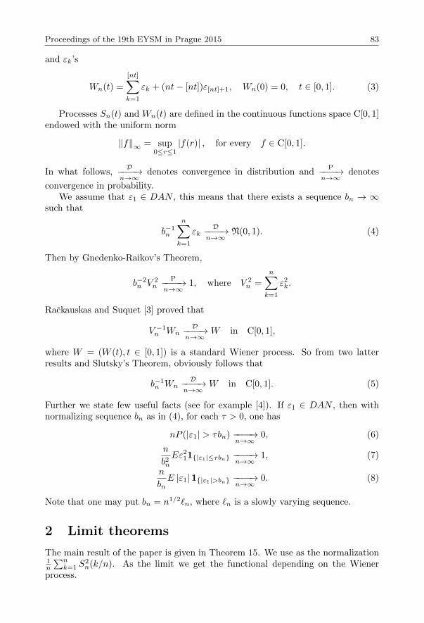
Proceedings of the 19th EYSM in Prague 2015 83
and εk’s
Wn(t) =
[nt]∑k=1
εk + (nt− [nt])ε[nt]+1, Wn(0) = 0, t ∈ [0, 1]. (3)
Processes Sn(t) and Wn(t) are defined in the continuous functions space C[0, 1]endowed with the uniform norm
‖f‖∞ = sup0≤r≤1
|f(r)| , for every f ∈ C[0, 1].
In what follows,D−−−−→
n→∞denotes convergence in distribution and
P−−−−→n→∞
denotes
convergence in probability.We assume that ε1 ∈ DAN , this means that there exists a sequence bn → ∞
such that
b−1n
n∑k=1
εkD−−−−→
n→∞N(0, 1). (4)
Then by Gnedenko-Raikov’s Theorem,
b−2n V 2
nP−−−−→
n→∞1, where V 2
n =
n∑k=1
ε2k.
Rackauskas and Suquet [3] proved that
V −1n Wn
D−−−−→n→∞
W in C[0, 1],
where W = (W (t), t ∈ [0, 1]) is a standard Wiener process. So from two latterresults and Slutsky’s Theorem, obviously follows that
b−1n Wn
D−−−−→n→∞
W in C[0, 1]. (5)
Further we state few useful facts (see for example [4]). If ε1 ∈ DAN , then withnormalizing sequence bn as in (4), for each τ > 0, one has
nP (|ε1| > τbn) −−−−→n→∞
0, (6)
n
b2nEε2
11|ε1|≤τbn −−−−→n→∞1, (7)
n
bnE |ε1|1|ε1|>bn −−−−→n→∞
0. (8)
Note that one may put bn = n1/2`n, where `n is a slowly varying sequence.
2 Limit theorems
The main result of the paper is given in Theorem 15. We use as the normalization1n
∑nk=1 S
2n(k/n). As the limit we get the functional depending on the Wiener
process.
84 Markeviciute -- Self-Normalized Limit Theorem for AR(1)
Theorem 15. Suppose (yk) is defined by (1) and (εk) are i.i.d. random variableswith ε1 ∈ DAN , Eε1 = 0, bn is defined by (4) and n(1− φn) −−−−→
n→∞∞, then
Sn√1n
∑nk=1 S
2n(k/n)
D−−−−→n→∞
W∫ 1
0W 2(s)ds
in C[0, 1]. (9)
To prove Theorem 15, we need few additional results that might be of inde-pendent interest. We start with the functional limit theorem in the continuousfunction space C[0, 1]. We prove that polygonal line process converge to Wienerprocess under the normalization (1− φn)/bn.
Theorem 16. Suppose (yk) is defined by (1) and (εk) are i.i.d. random variableswith ε1 ∈ DAN , Eε1 = 0, bn is defined by (4) and n(1− φn) −−−−→
n→∞∞, then
1− φnbn
SnD−−−−→
n→∞W in C[0, 1]. (10)
Next, we give another useful result.
Theorem 17. Suppose (yk) is defined by (1) and (εk) are i.i.d. random variableswith ε1 ∈ DAN , Eε1 = 0, bn is defined by (4) and n(1− φn) −−−−→
n→∞∞, then
1
n
n∑k=1
(1− φnbn
Sn(k/n)
)2D−−−−→
n→∞
∫ 1
0
W 2(s)ds. (11)
Finally we turn to a key point of the Theorem 16, that is to control the behaviourof max1≤k≤n |yk|.
Lemma 1. Suppose (yk) is defined by (1) and (εk) are i.i.d. random variableswith ε1 ∈ DAN , Eε1 = 0, bn is defined by (4) and n(1− φn) −−−−→
n→∞∞, then
b−1n max
1≤k≤n|yk| P−−−−→
n→∞0. (12)
3 Proofs
First we will prove Lemma 1.
Proof. Lemma 1. We need to prove
P (b−1n max
1≤k≤n|yk| > δ) −−−−→
n→∞0.
For this, let us introduce truncated random variables:
ε′j = εj1|εj |≤bn, εj = ε′j − Eε′jε′′j = εj1|εj |>bn, εj = ε′′j − Eε′′j .

Proceedings of the 19th EYSM in Prague 2015 85
Then we obtain
P (b−1n max
1≤k≤n|yk| > δ) ≤ nP (|ε1| > δbn) + P ′n,
where
P ′n = P
(b−1n max
1≤k≤n|y′k| > δ
)and y′k =
k∑j=1
φk−jn ε′j .
Now using (6), it only remains to show that P ′n −−−−→n→∞
0. For this we need to center
all ε′j and we get
P ′n ≤ P 1n + P 2
n ,
where
P 1n = b−1
n max1≤k≤n
∣∣∣∣∣∣k∑j=1
φk−jn Eε′j
∣∣∣∣∣∣ , P 2n = P
b−1n max
1≤k≤n
∣∣∣∣∣∣k∑j=1
φk−jn εj
∣∣∣∣∣∣ > δ
.
Note that Eε′j = Eε′′j , so
P 1n = b−1
n max1≤k≤n
∣∣∣∣∣∣k∑j=1
φk−jn Eε′′j
∣∣∣∣∣∣ ≤ E |ε′′1 | b−1n max
1≤k≤n
∣∣∣∣∣∣k∑j=1
φk−jn
∣∣∣∣∣∣≤ E |ε1|1|ε1|>bnb−1
n (1− φn)−1 =n
bnE |ε1|1|ε1|>bn · (n(1− φn))−1 −−−−→
n→∞0,
because of the conditions (8) and n(1− φn) −−−−→n→∞
∞.
Next let us turn to P 2n . Notice that E(ε1)2 ≤ 4Eε2
11|ε1|≤bn, so we obtain
P 2n ≤
1
b2nδ2E
max1≤k≤n
∣∣∣∣∣∣k∑j=1
φk−jn εj
∣∣∣∣∣∣2
≤ 1
b2nδ2
max1≤k≤n
k∑j=1
φ2(k−j)n E(εj)
2
≤ E(ε1)2
b2nδ2
(1− φ2n)−1 ≤ Cb−2
n (1− φn)−1Eε211|ε1|≤bn
= Cn
b2nEε2
11|ε1|≤bn(n(1− φn))−1 −−−−→n→∞
0,
where C is a constant and convergence follows from conditions n(1−φn) −−−−→n→∞
∞and (7). So the proof is finished.
Now we are ready to prove Theorem 16.
Proof. Theorem 16. We have (1), then summing up both sides by k we obtain:
1− φnbn
[nt]∑k=1
yk = (y0 − y[nt])b−1n + b−1
n
[nt]∑k=1
εk.

86 Markeviciute -- Self-Normalized Limit Theorem for AR(1)
Taking into account (5) we obtain that it is enough to prove∥∥∥∥1− φnbn
Sn −1
bnWn
∥∥∥∥∞
P−−−−→n→∞
0.
It is easy to see∥∥∥∥1− φnbn
Sn −1
bnWn
∥∥∥∥∞
= sup0≤r≤1
∣∣φn(y0 − y[nr])b−1n
∣∣ ≤ max0≤k≤n
∣∣φnb−1n (y0 − yk)
∣∣ .Note that |φn| ≤ 1, ∀n, also y0 = 0 and
b−1n max
1≤k≤n|yk| P−−−−→
n→∞0
by Lemma 1, so the proof is finished.
The proof of Theorem 17 is based on the integral approximation by sums.
Proof. Theorem 17. Let us denote
Z1n =
1
n
n∑k=1
(1− φnbn
Sn(k/n)
)2
and Z2n =
∫ 1
0
(1− φnbn
Sn(t)
)2
dt.
Then we have for any function f ∈ C[0, 1]∣∣∣∣∣ 1nn∑k=1
f(k/n)−∫ 1
0
f(s)ds
∣∣∣∣∣ =
∣∣∣∣∣n∑k=1
∫ k/n
(k−1)/n
(f(k/n)− f(s))ds
∣∣∣∣∣≤
n∑k=1
∫ k/n
(k−1)/n
|f(k/n)− f(s)|ds ≤ ω0
(f,
1
n
),
where ω0
(f, 1
n
)is modulus of continuity defined by
ω0
(f,
1
n
)= sup|t−s|≤1/n
|f(t)− f(s)| .
So we have ∣∣Z1n − Z2
n
∣∣ ≤ 1
nω0
((1− φnbn
Sn(t)
)2
, 1
).
By Theorem 16 we have that(
1−φnbn
Sn(t))
is tight, thus∣∣Z1n − Z2
n
∣∣ P−−−−→n→∞
0.
Finally, since integral is a continuous function, so we have by Theorem 17
Z2n
D−−−−→n→∞
∫ 1
0
W 2(s)ds
and the proof is finished.
Proceedings of the 19th EYSM in Prague 2015 87
Finally we can prove the main result.
Proof. Theorem 15. The result (9) follows from Theorems 16 and 17 and a contin-uous mapping theorem. Note that (9) exclude the degenerated case P (ε1 = 0) = 1,so that almost surely
∑nk=1 S
2n(k/n) > 0 for large enough n. To use continuous
mapping theorem correctly, let us define functional
F (x)(t) =x(t)√∫ 1
0x2(s)ds
and denote DF the set of discontinuity points of F . We need to show that P (W ∈Df ) = 0. For F the only possible discontinuities appears when X = 0, thusP (W ∈ Df ) = 0 is equivalent to P (W = 0) = 0 and this is a well known result. Sothe proof is finished.
References
[1] L. Giraitis and P. Phillips. Uniform limit theory for stationary autoregression.Journal of time series analysis, 27(1):51–60, 2006.
[2] J. Markeviciute, and A. Rackauskas, and Ch. Suquet. Functional limit theoremsfor sums of nearly nonstationary processes. Lithuanian Mathematical Journal,52(3):282–296, 2012.
[3] A. Rackauskas, and Ch. Suquet. Invariance principles for adaptive self-normalized partial sums processes. Stochastic Processes and their Applications,95(1):63–81, 2001.
[4] A. Rackauskas, and Ch. Suquet. Functional central limit theorems for self-normalized partial sums of linear processes. Lithuanian Mathematical Journal,51(2):251–259, 2011.
ICA Based on Fourth Moments
Jari Miettinen∗1, Klaus Nordhausen2, Hannu Oja2 and Sara Taskinen1
1Department of Mathematics and Statistics, University of Jyvaskyla, Finland2Department of Mathematics and Statistics, University of Turku, Finland
Abstract: In independent component analysis it is assumed that the componentsof the observed random vector are linear combinations of latent independent ran-dom variables, and the aim is then to find an estimate for a transformation matrixback to these independent components. This paper summarizes some contents of[8], where the statistical properties of four well-known estimation procedures basedon the use of fourth moments are studied in detail.
Keywords: affine equivariance, FastICA, FOBI, JADE, kurtosis
AMS subject classifications: 62H05, 62H10, 62H12
1 Introduction
The basic independent component (IC) model assumes that the components of thep-variate observed vector xi are linear combinations of the p mutually independentlatent components of zi = (zi1, . . . , zip). The model is written as
xi = µ+ Ωzi, i = 1, . . . , n, (1)
and the full rank p×p matrix Ω is called the mixing matrix. The location vector µ isa nuisance parameter and the aim is, using only a random sampleX = (x1, . . . ,xn),to find an estimate of an unmixing matrix W such that Wx has independentcomponents. Then z and Wx would differ only by order, signs, and scales of thecomponents. General assumptions for the latent components to be identifiable are
(A1) the components zi1, . . . , zip of zi are independent,
(A2) second moments exist, E(zi) = 0 and E(ziz′i) = Ip, and
(A3) at most one of the components zi1, . . . , zip of zi has a normal distribution.
The last assumption is needed because of the fact that the components of anyorthogonal transformation of two independent Gaussian random variables are stillGaussian and mutually independent. The assumption on the existence of secondmoments can be replaced with some other way of fixing the scales of the compo-nents, see, e.g., [7]. When dealing with the fourth moments, (A2) is of course notrestrictive at all. For more discussion on model (1) and on more general IC models,see [6].
Under (A2), a natural first step is so called whitening, i.e., standardizationx→ xst = Σ−1/2(x−µ), where Σ = ΩΩ′ is the covariance matrix of the random
∗Corresponding author: [email protected]

Proceedings of the 19th EYSM in Prague 2015 89
variable x from model (1) . Then z = Uxst for some orthogonal matrix U =(u1, . . . ,up)
′. Thus after estimating Σ, the estimation problem is simplified to theestimation problem of an orthogonal matrix U only, and then W = UΣ−1/2.
In this paper we review the use of fourth moments in ICA [8]. Section 2 presentsfour well-known estimators and Section 3 displays statistical properties of one ofthem. The performance of the four estimators is discussed briefly in Section 4.
2 Estimators
2.1 Independent component functionals
In the following definition, the population quantity which we wish to estimate isdefined as the value of an independent component functional W (Fx), where Fxdenotes the distribution function of x.
Definition 4. The p× p matrix-valued functional W (F ) is said to be an indepen-dent component (IC) functional if (i) W (Fx)x has independent components in theIC model and (ii) W (Fx) is affine equivariant in the sense that
W (FAx+b) = W (Fx)A−1
for all nonsingular p× p matrices A and for all p-vectors b.
Notice that (ii) implies that in the independent component model, W (Fx)xdoes not depend on the specific choices of z and Ω, up to the signs and the orderof the components. The sample version is W (X) = W (Fn), where Fn denotes theempirical distribution function of X = (x1, . . . ,xn).
2.2 Univariate kurtosis and ICA
The classical kurtosis measures of a random variable x with mean µ and varianceσ2 are β = E
([x− µ]4
)/σ2 and κ = β−3. For standardized variable z = (x−µ)/σ,
then β = E(z4). Normally distributed x has κ = 0, and thus, the deviation of κfrom zero indicates non-normality of x. The succes of many ICA estimators is moti-vated heuristically by the central limit theorem, stating that a mixture of mutuallyindependent random variables is more normal than the original variables, and theidea is to find such orthogonal U that the components of Uxst are maximallynon-normal. When the fourth moments are used as the measure of non-normality,the consistency of estimators can be proved as in the following theorem, see [8].
Theorem 18. Let the components of z = (z1, . . . , zp)′ be independent and stan-
dardized so that E(z) = 0 and Cov(z) = Ip, and assume that at most one of thekurtosis values κi = E(z4
i )−3, i = 1, . . . , p, is zero. Then the following inequalitieshold true.
(i) |E((u′z)4)− 3| ≤ max|E(z4
1)− 3|, . . . , |E(z4p)− 3|
for all u such that u′u = 1. The equality holds only if u = ei for i such that|E(z4
i )− 3| = max|E(z4
1)− 3|, . . . , |E(z4p)− 3|
, and
(ii) |E[(u′1z)4]− 3|+ · · ·+ |E[(u′pz)4]− 3| ≤ |E[z41 ]− 3|+ · · ·+ |E[z4
p]− 3|

90 Miettinen, Nordhausen, Oja and Taskinen -- ICA Based on Fourth Moments
for all orthogonal matrices U = (u1, . . . ,up)′. The equality holds only if U = JP
for some sign-change matrix J and permutation matrix P .
Items (i) and (ii) suggest the deflation-based [4] and symmetric [5] FastICAfunctionals, respectively.
Definition 5. The deflation-based FastICA functional is W (Fx) = UΣ−1/2,where Σ = Cov(x) and the rows of an orthogonal matrix U = (u1, . . . ,up)
′
are found one by one by maximizing |E((u′kxst)4) − 3| under the constraint that
u′kuk = 1 and u′juk = 0, j = 1, . . . , k − 1.
Definition 6. The symmetric FastICA functional is W (Fx) = UΣ−1/2, whereΣ = Cov(x) and U = (u1, . . . ,up)
′ maximizes
|E((u′1xst)4)− 3|+ . . .+ |E((u′pxst)
4)− 3|
under the constraint that UU ′ = Ip.
Later, new estimators with different non-normality measures have been intro-duced under the name of FastICA, but not all of them have been proved to beconsistent. If the sample size is small, finding the FastICA estimates is occasion-ally difficult due to convergence problems.
2.3 Multivariate kurtosis and ICA
Define, for any p× p matrix A, B(A) = E (xstx′stAxstx
′st), and further,
Bij = B(Eij), i, j = 1, . . . , p, and B = B(Ip) =
p∑i=1
Bii,
where Eij denotes the p× p matrix with ijth element one and others zero.The kurtosis matrix B is diagonal for xst = z with independent components,
and one of the earliest solutions to the independent component problem, FOBI(fourth order blind identification) [1], uses simultaneous diagonalization of the co-variance matrix Σ and the kurtosis matrix B.
Definition 7. The FOBI functional is W (Fx) = UΣ−1/2, where Σ = Cov(x) andthe rows of U are the eigenvectors of B = E (xstx
′stxstx
′st).
FOBI is a fast and simple method, but it has a major weakness that it isconsistent only if the kurtosis values of the independent components are distinct.
Unlike the kurtosis matrix B in FOBI, the matrices Bij are not diagonal atxst = z. However, the fourth order cumulant matrices
Cij = Bij −Eij − (Eij)′ − tr(Eij)Ip, i, j = 1, . . . , p,
are diagonal. The IC functional based on Joint Approximate Diagonalization ofthese (Eigen)matrices is called JADE [2], and it is defined as follows.

Proceedings of the 19th EYSM in Prague 2015 91
Definition 8. The JADE functional is W (Fx) = UΣ−1/2 where Σ = Cov(x) andthe orthogonal matrix U maximizes
p∑i=1
p∑j=1
||diag(UCijU ′)||2,
where diag(A) is a diagonal matrix with the same diagonal elements as A, and || · ||is the matrix norm.
The affine equivariance of the JADE estimate is not obvious, because the ma-trices Cij are not orthogonal equivariant. Interestingly, the joint diagonalizationof Cij , i, j = 1, . . . , p is orthogonal equivariant, which was rigorously proved in [8],and the affine equivariance of the estimate folllows.
There are several algorithms for an approximate diagonalization of several sym-metric matrices, but the statistical properties of the corresponding estimates arenot known. The most popular algorithm is perhaps the Jacobi rotation algorithmsuggested in [3]. It appeared in our simulations that the Jacobi rotation algo-rithm is computationally much faster and always provided the same solution asour algorithm based on the estimating equations, see Section 3.
The JADE estimate requires computation of p(p+ 1)/2 fourth moment matri-ces, which means that the computational load grows quickly with the number ofcomponents. Recently, a faster and asymptotically equivalent estimate with JADEwas found in [9], where the joint use of third and fourth moments in ICA wasstudied. The squared symmetric FastICA is obtained, when the absolute values ofthe regular symmetric FastICA are replaced by squares, i.e., we maximize, underthe orthogonality constraint,
(E((u′1xst)4)− 3)2 + . . .+ (E((u′pxst)
4)− 3)2.
3 Asymptotic properties of the JADE estimate
Let Z = (z1, . . . ,zn) be a random sample from a distribution satisfying (A1), (A2),and in addition to (A3), at least one of the following assumptions.
(A4) The fourth moments of z exist, and at most one of the kurtosis values κk =E(z4
ik), k = 1, . . . , p, is zero.
(A5) The fourth moments of z exist and are distinct.
For the independent components zik, k = 1, . . . , p, write also γk = E(z3ik) and
σ2k = V ar(z3
ik).
The limiting distributions of all four unmixing matrix estimates based on fourthmoments depend on the joint limiting distribution of
√n skl =
1√n
n∑i=1
zikzil and√n rkl =
1√n
n∑i=1
(z3ik − γk)zil,

92 Miettinen, Nordhausen, Oja and Taskinen -- ICA Based on Fourth Moments
k 6= l = 1, . . . , p. For the FOBI estimate we would also need
√n rmkl =
1√n
n∑i=1
z2imzikzil,
for distinct k, l,m = 1, . . . , p.
The JADE estimate is W = UΣ−1/2, where U solves the estimating equationsu′iT (uj) = u′jT (ui) and u′iuj = δij , i, j = 1, . . . , p. Here δij is the Kroneckerdelta and
T (u) =
p∑i=1
p∑j=1
(u′Ciju)Ciju.
The following theorem for the JADE estimate was given in [8], where you canalso find the corresponding results for the other estimates, and the references to
the articles where they were first given in. We consider the distribution of W =W (Z), i.e., the case Ω = Ip. Due to affine equivariance of the estimate, we haveW (X) = W (Z)Ω−1 in the general case.
Theorem 19. Let Z = (z1, . . . ,zn) be a random sample from a distribution ofz with bounded eighth moments satisfying the assumptions (A1), (A2) and (A4).
Then there is a sequence of solutions W such that W →P Ip and
√n (wkk − 1) = −1/2
√n (skk − 1) + oP (1), k = l, and
√n wkl =
κk√n rkl − κl
√n rlk +
(3κl − 3κk − κ2
k
)√n skl
κ2k + κ2
l
+ oP (1),
k 6= l.
Notice that the limiting distribution of√n wkl depends only on kth and lth
independent components. This holds true also for deflation-based and symmetricFastICA. On the contrary,
√n wkl of the FOBI estimate depends also on the other
components through√n rmkl, m 6= k, l. The limiting distributions of the diagonal
elements are the same for all four estimates.Under the assumptions of Theorem 19, the central limit theorem gives the
asymptotic normality of the estimate, and the componentwise asymptotic variancesare
ASV (wkk) = (κk + 2)/4, and
ASV (wkl) =(κ2k + κ2
l
)−2 (κ2k(σ2
k − κ2k − 6κk − 9) + κ2
l (σ2l − 6κl − 9)
), k 6= l
Since the effect of the term√n rmkl is rather minor in FOBI, the comparison of
the estimates can be reduced to the comparison of the sum ASV (wkl) +ASV (wlk)for selected kth and lth component distributions.
4 Comparison of the estimates
Besides the fact that JADE and squared symmetric FastICA are asymptoticallyequivalent, we have the following facts, when Ω = Ip.

Proceedings of the 19th EYSM in Prague 2015 93
1.√n wkl of the symmetric FastICA estimate and that of the JADE estimate are
asymptotically equivalent if the kth and lth marginal distributions are the same,2. If the independent components are identically distributed, then the symmetricFastICA and JADE estimates are asymptotically equivalent. In this case, the sumof the asymptotic variances of the off-diagonal elements is one half of that of thedeflation-based FastICA estimate. The FOBI estimate fails in this case.3. ASV (wkl) of the FOBI estimate is always larger than or equal to that forsymmetric FastICA, k 6= l. The variances are equal when p = 2 and κk > 0 > κl.4.√n wkp of the deflation-based FastICA estimate and of the JADE estimate are
asymptotically equivalent if the pth marginal distribution is normal.
Wide comparisons of the asymptotic variances in [8] expressed that JADE andthe symmetric FastICA perform best in most cases, and their asymptotic variancesare quite close to each other. The main difference between these two estimatorsappears when one of the components has a normal distribution. Then JADEoutperforms symmetric FastICA.Acknowledgements: This research was supported by the Academy of Finland(grants 251965, 256291 and 268703).
References
[1] J. F. Cardoso. Source separation using higher order moments. Proceedings of IEEEInternational Conference on Accoustics, Speech and Signal Processing, Glasgow, UK,2109–2112, 1989.
[2] J.F. Cardoso and A. Souloumiac. Blind beamforming for non Gaussian signals. IEEProceedings-F, 140:362–370, 1993.
[3] D. B. Clarkson. A least squares version of algorithm AS 211: The F-G diagonalizationalgorithm. Applied Statistics, 37:317–321, 1988.
[4] A. Hyvarinen and E. Oja. A fast fixed-point algorithm for independent componentanalysis. Neural Computation, 9:1483–1492, 1997.
[5] A. Hyvarinen. Fast and robust fixed-point algorithms for independent componentanalysis. IEEE Transactions on Neural Networks, 10:626–634, 1999.
[6] A. Hyvarinen, J. Karhunen, and E. Oja. Independent Component Analysis. JohnWiley and Sons, New York, 2001.
[7] P. Ilmonen and D. Paindaveine. Semiparametrically efficient inference based on signedranks in symmetric independent component models. The Annals of Statistics, 39:2448–2476, 2011.
[8] J. Miettinen, S. Taskinen, K. Nordhausen, and H. Oja. Fourth moments and inde-pendent component analysis. Accepted for publication in Statistical Science. Preprintavailable as arXiv, 2015.
[9] J. Virta, K. Nordhausen, and H. Oja, Joint use of third and fourth moments inindependent component analysis. Submitted, 2015.

Computational Aspects of Parameter Estimationin Ordinary Differential Equation Systems
Frederik Riis Mikkelsen∗
Department of Mathematical Sciences, University of Copenhagen, Denmark
Abstract: Ordinary differential equation (ODE) systems are widely applicable inmany branches of the natural sciences. They are especially valuable for analysingentire networks of processes with no internal noise. Though simple from a statis-tical point of view, the applicability of these models are usually hindered by theircomputational complexity. In this work I present a selection of current methodsto cope with the computational aspects of estimating parameters in ODE systems.Based on some of these methods, I present an algorithm for finding maximumlikelihood estimates (MLE) with certain computational qualities.
Keywords: ODE systems, parameter estimation, non-linear least squares, com-putational statistics
AMS subject classifications: 62J02
1 Introduction
We have in mind a d-dimensional ordinary differential equation system:
x = f(x, θ), x ∈ Rd (1)
parametrised by a p-dimensional vector θ ∈ Rp. For given θ, a solution to (1) is afunction ψθ : R→ Rd, such that
ψθ(t) = ψθ(0) +
∫ t
0
f(ψθ(s), θ) ds, for all t ∈ R. (2)
We observe the state of the system at discrete time points 0 = t1 < t2 < ... < tnwith independent Gaussian noise:
yj = ψθ(tj) + εj , εji.i.d.∼ N (0, σ2Id) (3)
for j = 1, ..., n. The negative log-likelihood is directly available (σ2 is omitted):
`y(θ) =1
2
n∑j=1
‖yj − ψθ(tj)‖22. (4)
This modelling framework for ODE systems is therefore quite simple from a statis-tical point of view. However, as explained below, optimising (4) is rather difficultfrom a computational angle.
∗Corresponding author: [email protected]

Proceedings of the 19th EYSM in Prague 2015 95
2 The optimisation problem
Finding the maximum likelihood estimator reduces to solving a non-linear leastsquares problem, due to (4). However, evaluating the likelihood requires solutionsof the underlying ODE system. Various numerical methods for finding approxima-tive solutions exist, but are relatively time consuming. Specifically, employing anexplicit Runge-Kutta scheme of size s (see e.g. section 17 in [5] for details) thenumber of evaluations of f is sT
δ . Here δ is the step size and T is the time span. Forsuch a scheme the global truncation error is O (Tδp), for some scheme-dependentp ≤ s. Using an implicit Runge-Kutta scheme, instead, leads to a smaller globaltruncation error, but raises the number of evaluations of f and is O
(dsTδ
)in best
case scenarios.The number of f -evaluations is substantial for assessing the computational com-
plexity of evaluating `y. Though linear in each variable (considering 1/δ as mea-suring the mesh), the number of f -evaluations is typically large. Consequently, inorder to optimise (4) efficiently, a minimal number of evaluations of `y is prefer-able, especially when the observed time points cover a large time span or the ODEsystem is stiff.
3 Methods
3.1 Gauss-Newton approach (shooting)
From a numerical optimisation perspective, `y has the valuable property of beinga sum of squares. Thus the classical Gauss-Newton algorithm is typically a firstchoice for the optimisation scheme. The Gauss-Newton algorithm has the samerate of convergence as most second order approximation algorithms, but requiresno computations of the hessian matrix (see e.g. section 10 in [6] for details).However, calculating the gradient of `y:
∇θ`y(θ) = −n∑j=1
(yj − ψθ(tj))′Dθψ(tj) (5)
amounts to deriving Dθψ. This differential is typically only available as a solutionto the matrix differential equation system
˙Dθψ =∂f
∂x(ψ(t), θ)Dθψ +
∂f
∂θ(ψ(t), θ). (6)
Consequently, employing the Gauss-Newton algorithm requires solving (1) and (6)simultaneously at each step. Using an explicit Runge-Kutta scheme of size s, thisamounts to evaluating f , ∂f
∂x and ∂f∂θ , sT
δ times at each step of the optimisation.Subsequently, for large and complex systems, evaluating the gradient of `y is eitherextremely time consuming or close to impossible.
There are numerous variations of the above approach (see, e.g., [3] for a moresophisticated version). They are often referred to as shooting methods, inspiredby the shooting method from boundary value problems. These methods typically

96 Mikkelsen -- Parameter Estimation in Differential Equation Systems
rely on general optimisation algorithms and will therefore not exploit all essentialfeatures of ODE systems. The remaining algorithms incorporate these features byconsidering, e.g., the functional nature of the data.
3.2 Generalised smoothing approach (collocation)
Certain implicit Runge-Kutta schemes are so-called collocation methods. Theyrely on the principle that an approximative solution to (1) can be found in somefinite dimensional function space, typically spanned by a set of spline functions.The collocation method therefore amounts to finding an element of the functionspace that satisfy (1) in some pre-specified time points, called collocation points.This approach is the inspiration to various parameter estimation methods in ODEsystems. The following method is due to Ramsay et. al, see [4]:
This approach relies on the approximation of ψθ given by
ψθ(t) ≈ ϕ(t)′cθ for t ∈ [0, tn]. (7)
Here ϕ is a vector of univariate basis functions, which combined with the vector cθof coefficients yields an approximative solution to (1). The parameter dependenceθ 7→ ψθ is therefore passed on to θ 7→ cθ. The least squares criterion:
J(c, θ) =∑j
‖yj − ϕ(tj)′c‖22 + λ
∫ tn
t1
‖ϕ(t)′c− f(ϕ(t)′c, θ)‖22 dt (8)
is proposed, where λ > 0 is a tuning parameter shifting the weight between thedata fitting criterion and the so-called fidelity measure of ϕ′c. Applying profilingmethods to (8), cθ appears as the minimum of c 7→ J(c, θ). If f is linear in x, theminimisation problem reduces to a linear least squares problem, thus providing ananalytical expression for θ 7→ cθ.
By introducing this approach, some of the tools of functional data analysis issuddenly available, which provide new insightful views on the estimation problem.However, it is worth considering the influence of the choice of ϕ on the inference.Moreover, the relation between optimising a family of semi-norms parametrised byλ (the criterion J in (8)) and the actual MLE defined through (4) is not completelyclear. Finally, for non-linear systems, optimising c 7→ J(c, θ) and θ 7→ J(cθ, θ) usinggradient based methods still require evaluating ∂f
∂x and ∂f∂θ many times (depending
on how the integral in (8) is approximated).
3.3 Gradient/integral matching
The core principle of this method is: if the whole noiseless curve ψ is observed,then θ can be inferred by minimising
∫ tn
t1
∥∥∥ψ(t)− f(ψ(t), θ)∥∥∥2
2dt, or
∫ tn
t1
∥∥∥∥ψ(t)− ψ(t1)−∫ t
t1
f(ψ(s), θ)ds
∥∥∥∥2
2
dt. (9)

Proceedings of the 19th EYSM in Prague 2015 97
We therefore consider the estimator, that takes a non-parametric estimate of ψ, ψ,and returns the value of θ minimising (9):
ψ 7→ arg minθ
∫ tn
t1
∥∥∥∥ψ(t)− ψ(t1)−∫ t
t1
f(ψ(s), θ)ds
∥∥∥∥2
2
dt. (10)
If ψ(t1) is unknown, it can be included in the parameter vector θ. In [1] the authorproves that if the above map is applied to a consistent non-parametric estimator,the resulting estimator of θ is also consistent, under mild regularity assumptions.Additionally, he also finds conditions for asymptotic normality.
This approach truly flourishes when applied to systems in which f is linear inθ (and not necessarily linear in x). In such cases (10) reduces to a linear leastsquares problem, which can be solved even for very large and complex systems,i.e., for large n and p. Furthermore, one can introduce, e.g., `1-penalties to (10)and apply the method to systems with p >> nd and still have computationallystable methods for finding solutions.
Brewer et al. ([2]) proposed an iterative procedure exploiting the qualities ofthis type of gradient matching. More precisely, they consider a fitting criterionresembling that of [4]:∑
j
‖yj − ϕ(tj)′c‖22 + λ
∑r
‖ϕ(tr)′c− f(ϕ(tr)
′c, θ)‖22 (11)
where r is allowed to run over a finer (or coarser) grid than j. The iterations consistof letting c be fixed and then estimate (c, θ) as the linear least squares estimates of(11). The estimate of c then enters as c in the next iteration. By applying gradient
matching iteratively one avoids choosing a specific ψ, as opposed to a non-iterativegradient matching.
Similarly to the generalised smoothing approach, this method has the followingimportant strength: the optimisation problem and the ODE-solution problem areseparated. Thus evaluating the fitting criterion is inexpensive and evaluating thegradient (typically) requires less calculations of ∂f
∂x and ∂f∂θ .
The method described above is applicable to many non-trivial systems and canhandle large and sparse models. However, there are things to consider: the iterativeprocedure is still dependent on the choice of ϕ. It is also unclear how optimisingthe criterion (11) is related to the MLE given through (4). Finally, it is nontrivialwhether this sequence of iterative estimates of (c, θ) converge to the optimum of(11) (if it converges at all).
4 Combining algorithms
Returning to the original problem of minimising (4), we required relatively fewevaluations of `y and ∇`y. In this section we consider a new algorithm based onthe above, which yields the actual MLE (a quality of the shooting methods) andstill exploits the computationally attractive aspects of gradient matching.
Firstly, given a current estimate of θ, denoted θk in the iterative procedure, wecalculate an approximative solution curve ψθk . Then we perform integral matching

98 Mikkelsen -- Parameter Estimation in Differential Equation Systems
Initialisation:k = 0
θ0 provided
DescentDirection:
Find descentdirection pk, e.g.,Gauss-Newton
Stop‖pk‖ < δ
Backtracking:Find backtrackingconstant α, e.g.,via line search
‖pk‖ ≥ δ
Update:k := k + 1
θk := θk + αpk
Initialisation:k = 0
θ0 provided
Oracle:Find oracledirection pok.Set pk = pok.
DescentDirection:
Find descentdirection pk, e.g.,Gauss-Newton
‖pk‖ < δStop
‖pk‖ < δ
Backtracking:Find backtrackingconstant α, e.g.,via line search
‖pk‖ ≥ δ‖pk‖ ≥ δα < ε
Update:k := k + 1
θk := θk + αpk
α ≥ ε
Figure 1: Flowcharts of a generic line search algorithm with and without an oracle.
between the curve and the observations. The resulting estimate of θ:
θoraclek = arg min
θ
n∑j=1
∥∥∥∥yj − ψ(t1)−∫ tj
t1
f(ψθk(s), θ)ds
∥∥∥∥2
2
. (12)
is called the oracle estimate. We denote poraclek = θoracle
k − θk the oracle direction.In general it is not certain that `y(θoracle
k ) < `y(θk), hence a backtracking of poraclek
must be employed in order to gain a descent:
θk+1 = θk + αporaclek
for some α ∈ [0, 1]. However, it is not even certain that poraclek is a descent direction!
In which case, the backtracking will fail to find a positive α within numericaltolerance. In this case, no benefit from the oracle is gained. The algorithm thenpasses on to some classic optimisation scheme, e.g., Gauss-Newton. Once a singleGauss-Newton update is done, the algorithm returns to the oracle for the nextiterate. A generic line search optimisation algorithm with and without an oracleare visualised by two flowcharts in figure 1.
This algorithm maintains the convergence properties of the Gauss-Newton al-gorithm, while benefiting from computational advantages possessed by the oracle.In practice the oracle mostly provides excellent descent directions and the Gauss-Newton part will only be invoked to verify that the final iterate is an approximativelocal minima.

Proceedings of the 19th EYSM in Prague 2015 99
5 Discussion and further work
The new combined algorithm presented above has been implemented and tested onsimulated data from mass action kinetics models. The results look promising bothfor large and small σ2, along with high and low frequency data. In these studies theoracle always provided a descent direction. Intuitively this is not true in general, asthe algorithm will perform poorly for stiff or chaotic systems. The computationallyheavy part of the algorithm is the Gauss-Newton part. Consequently, it is ofhigh interest to find conditions that ensure the oracle alone provides the descentdirections necessary to find MLE.
Additionally, the algorithm can be extended to parameter estimation withforced sparsity, e.g., using `p penalties. This is relevant for estimating unknownmodel structures. However, when introducing such penalties the algorithm has tobe revised in order to accommodate potential lack of smoothness.
Acknowledgements: A great thanks to Professor Niels Richard Hansen and Mar-tin Vincent of Department of Mathematical Sciences at University of Copenhagenfor guidance and many insightful discussions.
References
[1] N. J-B. Brunel. Parameter estimation of ODE’s via nonparametric estimators.Electronic Journal of Statistics, 2:1242–1267, 2008.
[2] D. Brewer, M. Barenco, R. Collard, M. Hubank and J. Stark. Fitting ordinarydifferential equations to short time course data. Philos. Transact. A Math.Phys. Eng. Sci., 366:519–544, 2008.
[3] Z. Li, M. R. Osborne and T. Prvan. Parameter estimation of ordinary differ-ential equations. IMA Journal of Numerical Analysis, 25(2):264–285, 2005.
[4] J. O. Ramsay, G. Hooker, D. Campbell and J. Cao. Parameter estimation fordifferential equations: a generalised smoothing approach. J. R. Statist. Soc. B,69(5):741–796, 2007.
[5] W. H. Press, B. P. Flannery, S. A. Teukolsky and W. T. Vetterling. NumericalRecipes: The Art of Scientific Computing (3rd ed). Cambridge University Press,2007.
[6] J. Nocedal and S. J. Wright. Numerical Optimization (2nd ed). Springer, 2006.

On Calculation of the Integrals Depending on aParameter by Monte-Carlo Method
Yuriy Mlavets∗1 and Yuriy Kozachenko2
1Uzhhorod National University, Ukraine2Taras Shevchenko National University of Kyiv, Ukraine
Abstract: In this work we use the theory Fψ(Ω) spaces in order to find theaccuracy and reliability for the calculation of the improper integrals depending ona parameter t by Monte Carlo method.
Keywords: Fψ(Ω) space of random variables, condition H, Monte Carlo method,stochastic process
AMS subject classifications: 65C05, 60G07
1 Introduction
In this paper we developed a theory for finding the reliability and accuracy forthe calculation of integrals depending on a parameter by Monte-Carlo method inLp(T ) metrics.
There are many works devoted to the usage of the Monte-Carlo methods forcalculation of integrals. Among them are the books by Yermakov [1] and Yermakov& Mikhailov [2].
The paper by Kurbanmuradov & Sabelfeld [7] contains the estimate for theaccuracy in the space C(T ) and reliability for the calculation of integrals dependingon a parameter if the set of integration is bounded. To obtain these results thetheory of sub-Gaussian processes had been used.
The space Fψ(Ω) was introduced by Yermakov & Ostrovsky in the paper [3].The paper [5] is devoted to studying the properties of such spaces and there hadbeen found the conditions of fulfilling the condition H (see Definition 10) in thisspaces. The condition H is necessary for finding the reliability and accuracy whenwe calculate integrals by Monte-Carlo method.
The choice of the space depends on particular integral and allows to find betteraccuracy. In this paper, the accuracy is defined via the norm in Lp(T ) space.
2 Fψ(Ω) – space
Definition 9. [6] Let ψ(u) > 0, u ≥ 1 be monotonically increasing, continuousfunction for which ψ(u)→∞ as u→∞. A random variable ξ belongs to the spaceFψ(Ω) if
supu≥1
(E |ξ|u)1/u
ψ(u)<∞.
∗Corresponding author: [email protected]

Proceedings of the 19th EYSM in Prague 2015 101
The similar definition was formulated in the paper by S. M. Yermakov & Ye. I.Ostrovskii [3]. But there was required that Eξ = 0 as ξ ∈ Fψ(Ω). Moreover, therewere considered the random variables for which E |ξ|u =∞ for some u > 0.
It had been proved in [3] that Fψ(Ω) is a Banach space with a norm
‖ξ‖ψ = supu≥1
(E |ξ|u)1/u
ψ(u).
Theorem 20. [6] If a random variable ξ belongs to the space Fψ(Ω), then for anyε > 0 the following inequality holds true:
P |ξ| > ε ≤ infu≥1
‖ξ‖uψ (ψ(u))u
εu.
Theorem 21. [6] If a random variable ξ belongs to the space Fψ(Ω) and ψ(u) =uα, where α > 0, then for any ε ≥ eα ‖ξ‖ψ the following inequality is true:
P |ξ| > ε ≤ exp
−αe(
ε
‖ξ‖ψ
)1/α .
Definition 10. [5] We say that the condition H for the Banach spaces B(Ω) ofrandom variables is fulfilled if there exists such an absolute constant CB that for anycentered and independent random variables ξ1, ξ2, . . . , ξn from B(Ω) the followingis true: ∥∥∥∥∥
n∑i=1
ξi
∥∥∥∥∥2
≤ CBn∑i=1
‖ξi‖2 .
The constant CB is called a scale constant for the space B(Ω). For space Fψ(Ω)we shall denote the constants CFψ(Ω) as Cψ.
Theorem 22. [8] For the space Fψ(Ω), where ψ(u) = uα, α ≥ 12 the condition H
is fulfilled and it is true the following inequality:∥∥∥∥∥n∑i=1
ξi
∥∥∥∥∥2
ψ
≤ 4 · 9αn∑i=1
‖ξi‖2ψ .
Note, that when α < 12 then the condition H is not fulfilled for this space.
3 Estimates in the norm Lp(T ) for the stochasticprocesses from the spaces Fψ(Ω)
Theorem 23. Let ν be the σ-finite measure on the compact metric space (T, ρ)and X = X(t), t ∈ T be a measurable stochastic process from the space Fψ(Ω).If for some p ≥ 1 the following condition is true∫
T
‖X(t)‖pψ dν(t) <∞,
then

102 Mlavets and Kozachenko -- On Calculation of the Integrals
1) the integral∫T
|X(t)|p dν(t) exists with probability one and the inequality holds
true: ∥∥∥∥∥∥∥∫T
|X(t)|p dν(t)
1/p∥∥∥∥∥∥∥ψ
≤ ψ(p)
ψ(1)
∫T
‖X(t)‖pψ dν(t)
1/p
;
2) for any ε > 0 the following inequality holds:
P
∫T
|X(t)|p dν(t)
1/p
> ε
≤
≤ infu≥1
(ψ(p)ψ(1)
)u(∫T
‖X(t)‖pψ dν(t)
)u/p(ψ(u))u
εu.
Example 1. Consider the space Fψ(Ω), where ψ(u) = uα, α > 0. It follows from
the Theorems 23 and 21 that for ε ≥ (ep)α(∫T
‖X(t)‖pψ dν(t)
)1/p
P
∫T
|X(t)|p dν(t)
1/p
> ε
≤
≤ exp
−α
ep
ε(∫T
‖X(t)‖pψ dν(t)
)1/p
1/α .
Theorem 24. Let ν be a σ-finite measure on a compact metric (T, ρ) and Y =Y (t), t ∈ T be the stochastic process from the space Fψ(Ω) and the conditionH is fulfilled for this space with the constant Cψ. Let EY (t) = m(t), Zn(t) =
1n
n∑k=1
Yk(t) −m(t) = 1n
n∑k=1
(Yk(t) −m(t)), where Yk(t) are the independent copies
of Y (t). Then the following inequality holds for all p ≥ 1
∥∥∥∥∥∥∥∫T
|Zn(t)|p dν(t)
1/p∥∥∥∥∥∥∥ψ
≤ 2√Cψ√n· ψ(p)
ψ(1)
∫T
‖Y (t)‖pψ dν(t)
1/p
Proceedings of the 19th EYSM in Prague 2015 103
and for every ε > 0 the following estimate is true
P
∫T
|Zn(t)|p dν(t)
1/p
> ε
≤
≤ infu≥1
(2√Cψ√n· ψ(p)ψ(1)
)u(∫T
‖Y (t)‖pψ dν(t)
)u/p(ψ(u))u
εu.
Example 2. Let us consider the space Fψ(Ω), where ψ(u) = uα, α > 0 then it
follows from the Theorems 24 and 21 that if ε ≥ (ep)α2√Cψ√n
(∫T
‖Y (t)‖pψ dν(t)
)1/p
P
∫T
|Zn(t)|p dν(t)
1/p
> ε
≤
≤ exp
−α
ep
ε
2√Cψ√n
(∫T
‖Y (t)‖pψ dν(t)
)1/p
1/α .
4 Reliability and accuracy in the space Lp(T ) forthe calculation of integrals depending on a pa-rameter
Let S,A, µ be a measurable space, µ be a σ-finite measure and p(s) ≥ 0, s ∈ S besuch measurable function that
∫Sp(s)dµ(s) = 1. Let m(A), A ∈ A be the measure
m(A) =∫A
p(s)dµ(s). m(A) is a probability measure and the space S,A,m is a
probability space.
Let us consider the integral∫Sf(s, t)p(s)dµ(s) = I(t) assuming that it exists.
Let the function f(s, t) depend on the parameter t ∈ T , where (T, ρ) is somecompact set and the function f(s, t) be continuous with regard to t.
Suppose f(s, t) is the stochastic process on S,A,m and we denote it asξ(s, t) = ξ(t) and I(t) =
∫Sf(s, t)p(s)dµ(s) =
∫Sf(s, t)dm(s) = Eξ(t).
Let ξi(t), i = 1, 2, . . . , n be the independent copies of the stochastic process
ξ(t), Zn(t) = 1n
n∑i=1
ξi(t). So, according to the strong law of large numbers Zn(t)→Eξ(t) = I(t) with probability one for any t ∈ T .

104 Mlavets and Kozachenko -- On Calculation of the Integrals
Definition 11. We say that Zn(t) approximates I(t) in the space Lp(T ) withreliability 1− δ > 0 and accuracy ε > 0 if the following inequality holds true:
P
∫T
|Zn(t)− I(t)|p dµ(t)
1/p
> ε
≤ δ.Theorem 25. Let I(t) = Eξ(t) =
∫Sf(s, t)p(s)dµ(s), ξ(t) be the stochastic process
which belongs to the space Fψ(Ω) satisfying the condition H with constant Cψ,
Zn(t) = 1n
n∑i=1
(ξi(t)− I(t)), ξi(t) be the independent copies of the stochastic process
ξ(t).Then, for all p ≥ 1 the following inequality holds true∥∥∥∥∥∥∥
∫T
∣∣∣Zn(t)∣∣∣p dµ(t)
1/p∥∥∥∥∥∥∥ ≤
2√Cψ√n· ψ(p)
ψ(1)
∫T
‖ξ(t)‖pψ dµ(t)
1/p
,
and Zn(t) approximates I(t) with reliability 1−δ and accuracy ε in the space Lp(T )for such n that
infu≥1
(2√Cψ√n· ψ(p)ψ(1)
)u(∫T
‖ξ(t)‖p dµ(t)
)u/p(ψ(u))u
εu≤ δ. (1)
Example 3. Consider the space Fψ(Ω), where ψ(u) = uα, α > 12 . Then the
Theorem 22 implies that the condition H is fulfilled for this space with the constantCψ = 4 · 9α. It follows from the Example 2 and the Theorem 25 that if ε ≥4(3pe)α
(∫T
‖ξ(t)‖pψdµ(t)
)1/p
√n
, then
infu≥1
(2√Cψ√n· ψ(p)ψ(1)
)u(∫T
‖ξ(t)‖p dµ(t)
)u/p(ψ(u))u
εu≤
≤ exp
−α
e
√nε
4(3pe)α(∫T
‖ξ(t)‖pψ dµ(t)
)1/p
1/α .
So, the inequality (1) holds if it is true that
exp
−α
e
√nε
4(3pe)α(∫T
‖ξ(t)‖pψ dµ(t)
)1/p
1/α ≤ δ,

Proceedings of the 19th EYSM in Prague 2015 105
as
n ≥
4(3pe)α
(∫T
‖ξ(t)‖pψ dµ(t)
)1/p
ε
2 (
(− ln δ)e
α
)2α
.
Then
n ≥
4(3p)α
(∫T
‖ξ(t)‖pψ dµ(t)
)1/p
ε
2
max
(1,
(− ln δ
α
)2α).
References
[1] S. M. Ermakov. The Monte Carlo Method and Contiguous Questions. Moscow,Nauka, 163, 1975.
[2] S. M. Ermakov and G. A. Mikhailov. The Course of Statistical Modelling.Moscow, Nauka, 319, 1976.
[3] S. V. Ermakov and E. I. Ostrovskii. Continuity conditions, exponential esti-mates, and the central limit theorem for random fields. Dep. VINITI, Moscow,3752-B.86.0:42, 1986.
[4] Yu. V. Kozachenko and Yu. Yu. Mlavets. Probability of large deviations of sumsof random processes from Orlicz space. Monte Carlo Methods Applications,17:155–168, 2011.
[5] Yu. V. Kozachenko and Yu. Yu. Mlavets. The Banach spaces Fψ(Ω) of randomvariables . Theory of Probability and Mathematical Statistics, 86:105–121, 2013.
[6] Yuriy Kozachenko and Yuriy Mlavets. Stochastic processes from Fψ(Ω) spaces.Contemporary Mathematics and Statistics, 2(1):55–75, 2014.
[7] O. Kurbanmuradov and K. Sabelfeld. Exponential bounds for the probabilitydeviations of sums of random fields. Monte Carlo Methods and Applications,12(3-4):211–229, 2006.
[8] Yu. Yu. Mlavets. A relationship between the spaces Fψ(Ω) and Orlicz spacesrandom variables. Scientific Bulletin of the Uzhhorod University. Series Math-ematics and Informatics, 25(1):77–84, 2014.

Behavior of Rank Tests and R-Estimates inMeasurement Error Models
Radim Navratil∗
Masaryk University, Brno, Czech Rep.
Abstract: Behavior of rank tests and R-estimates in presence of measurementerrors is studied. It is showed that rank tests of some hypotheses stay valid in mea-surement error models. The presence of measurement errors only decreases theirpower. Unlike that R-estimates in measurement error models are biased. Unfortu-nately this bias cannot be corrected without any knowledge of the distribution ofmeasurement errors.
Keywords: aligned rank tests, measurement error models, rank tests, R-estimates
AMS subject classifications: 62G10, 62G30
1 Introduction
Measurement error models (also called errors-in-variables models) are regressionmodels that account for measurement errors in the independent variables (regres-sors). These models occur very commonly in practical data analysis, where somevariables cannot be observed exactly, usually due to instrument or sampling error.Sometimes ignoring measurement error may lead to correct conclusions, howeverin some situations it may have dramatic consequences.
The most of the literature about measurement error models uses parametric ap-proach with its restrictive normality assumptions or a knowledge of some additionalinformation about error distribution (see e.g. [1]). We avoided this and introduceda class of rank tests that is valid even if measurement errors are present. The maingoal of this paper is to investigate the behavior of standard rank procedures inmeasurement error models - both tests and estimates. Proofs of the theorems areomitted, but they may be found in [3] and[4].
2 Behavior of rank tests in measurement errormodels
Consider classical linear regression model
Yi = β0 + x>i β + ei, i = 1, . . . , n, (1)
∗Corresponding author: [email protected]

Proceedings of the 19th EYSM in Prague 2015 107
where β0 ∈ R and β ∈ Rp are unknown parameters, model errors ei are assumedto be independent identically distributed (i.i.d.) with an unknown distributionfunction F and density f , xi are vectors of known regressors, such that
Qn =1
n
n∑i=1
(xi − x)(xi − x)>, with x =1
n
n∑i=1
xi
is a positive definite matrix (further on we will tacitly assume that this holds). Ouraim is to test the hypothesis H0 : β = 0 against K0 : β 6= 0.
Choose a nondecreasing, nonconstant, square integrable score generating func-tionϕ : (0, 1) 7→ R and define
an(i) = ϕ
(i
n+ 1
), i = 1, . . . , n,
A2(ϕ) =
∫ 1
0
(ϕ(t)− ϕ)2dt, ϕ =
∫ 1
0
ϕ(t)dt.
Let Ri be the rank of Yi among Y1, . . . , Yn and define vector of linear rankstatistics
Sn = n−1/2n∑i=1
(xi − x)an(Ri).
Test criterion for H0 is then
T 2n = A−2(ϕ)S>nQ−1
n Sn. (2)
Assume that f has finite Fisher information with respect to the location
0 < I(f) =
∫ (f ′(x)
f(x)
)2
f(x)dx <∞ (3)
and there exists a positive definite matrix Q, such that as n→∞
Qn → Q, (4)
1
nmax
i=1,...,n(xi − x)>Q−1
n (xi − x)→ 0. (5)
Remark 3. Generally, Fisher information is defined for parametric family d(x, θ)of densities as
I(d, θ) =
∫ ( ∂∂θd(x, θ)
d(x, θ)
)2
d(x, θ)dx.
If θ is a location parameter, i.e. d(x, θ) = f(x− θ), then I(d, θ) = I(f).
Theorem 26. Assume that (3) – (5) hold. Then in model (1) under H0 teststatistic T 2
n has asymptotically as n→∞ χ2 distribution with p degrees of freedomand under sequence of local alternatives
K0,n : β = n−1/2β∗, 0 6= β∗ ∈ Rp fixed

108 Navratil -- Rank Procedures in Measurement Error Models
T 2n has asymptotically as n→∞ noncentral χ2 distribution with p degrees of free-
dom and noncentrality parameter
η2 = β∗>Qβ∗γ2(ϕ, f)
A2(ϕ), γ(ϕ, f) =
∫ 1
0
ϕ(t)ϕ(t, f)dt, ϕ(t, f) = −f′(F−1(t))
f(F−1(t)).
2.1 Model with errors in regressors
Measurement error model assumes that regressors xi are not observed accurately,but only with an additive, unobservable, error vi, i.e. we observe wi = xi + viinstead of xi, where v1, . . . ,vn are i.i.d. random vectors independent of e1, . . . , en.In other words, we may write
Yi = β0 + x>i β + ei, (6)
wi = xi + vi, i = 1, . . . , n.
Denote T 2w,n test statistic (2) based on observed values (Yi,wi). It is easy
to show that T 2w,n has under H0 the same distribution as T 2
n . The presence ofmeasurement errors only decreases power of the test.
2.2 Aligned rank tests
However, we are often more interested in testing hypothesis only about a componentof the parameter β, identify regressors that have influence on response variable.Denote
β = (β>1 ,β>2 )>, xi = (x>1,i,x
>2,i)>,
vi = (v>1,i,v>2,i)>, wi = (w>1,i,w
>2,i)>,
where β1 ∈ Rp−q, β2 ∈ Rq, x1,i ∈ Rp−q, x2,i ∈ Rq, v1,i ∈ Rp−q, v2,i ∈ Rq,w1,i ∈ Rp−q, w2,i ∈ Rq, 1 ≤ q < p. Then model (6) can be rewritten as
Yi = β0 + x>1,iβ1 + x>2,iβ2 + ei,
w1,i = x1,i + v1,i, (7)
w2,i = x2,i + v2,i, i = 1, . . . , n.
Our goal is to test the hypothesis H1 : β2 = 0 against K1 : β2 6= 0, consideringβ0 and β1 as nuisance parameters.
Rank tests are invariant with respect to the location, but not to the nuisanceregression. That is why we have to first estimate the nuisance parameter β1 andthen apply the standard test on residuals. Due to the absence of knowledge ofdistribution of model errors and to preserve robust properties we use an R-estimatorof parameter β1.
Model (7) under H1 reduces to Yi = β0 + w>1,iβ1 + e∗i , where e∗i = ei − v>1,iβ1
are i.i.d. random variables with density f∗ = f∗β1.
Choose a nondecreasing, nonconstant, square integrable score generating func-tion ψ : (0, 1) 7→ R that is skew-symmetric, i.e. ψ(1− t) = −ψ(t), ∀ 0 < t < 1

Proceedings of the 19th EYSM in Prague 2015 109
and define an(i) = ψ(
in+1
), i = 1, . . . , n. Following [2] we define the rank
(pseudo)estimator β1,n of β1 as a minimizer of
Dn(b) =
n∑i=1
(Yi −w>1,ib
)an(Ri(b))
with respect to b ∈ Rp−q, where Ri(b) is the rank of (Yi −w>1,ib) among
(Y1 −w>1,1b), . . . , (Yn −w>1,nb).Now, consider residuals
ei = Yi −w>1,iβ1,n, i = 1, . . . , n
and apply the test described in Section 2 on residuals e1, . . . , en. Note that unlikethe situation in Section 2 residuals ei are not independent, because they depend onthe R-estimate of nuisance parameter β1. However under some assumptions thisfact does not affect the asymptotic distribution.
Hence choose a nondecreasing, nonconstant, square integrable score generating
function ϕ : (0, 1) 7→ R (it may differ from ψ) and define an(i) = ϕ(
in+1
), i =
1, . . . , n and compute
Sn = n−1/2n∑i=1
(w2,i −w2)an(Ri(β1,n)),
where Ri(β1,n) is the rank of ei among e1, . . . , en. Denote
D1,n =1
n
n∑i=1
(w1,i −w1)(w1,i −w1)>, D2,n =1
n
n∑i=1
(w2,i −w2)(w2,i −w2)>.
Finally, consider test statistic
T 2n = A−2(ϕ)S>nD−1
2,nSn.
Assume that there exist positive definite matrices Q1,Q2,C1,C2, such that
Q1,n =1
n
n∑i=1
(x1,i − x1)(x1,i − x1)> → Q1, (8)
C1,n =1
n
n∑i=1
(v1,i − v1)(v1,i − v1)>p→ C1, (9)
1
nmax
i=1,...,n(w1,i −w1)>D−1
1,n(w1,i −w1)→ 0, (10)
Q2,n =1
n
n∑i=1
(x2,i − x2)(x2,i − x2)> → Q2, (11)
C2,n =1
n
n∑i=1
(v2,i − v2)(v2,i − v2)>p→ C2, (12)
1
nmax
i=1,...,n(w2,i −w2)>D−1
2,n(w2,i −w2)→ 0. (13)

110 Navratil -- Rank Procedures in Measurement Error Models
Finally, we are able to describe asymptotic distribution of T 2n .
Theorem 27. Assume that (3), (8) – (13) hold. Then in model (7) under H1 test
statistic T 2n has asymptotically as n→∞ χ2 distribution with q degrees of freedom
and under local alternative
K1,n : β2 = n−1/2β∗2, 0 6= β∗2 ∈ Rq fixed
T 2n has asymptotically noncentral χ2 distribution with q degrees of freedom and
noncentrality parameter
η2 = β∗>2 Q2(Q2 + C2)−1Q2β∗2
γ2(ϕ, f∗)
A2(ϕ).
Recall that f∗ depends on unknown nuisance parameter β1 and distribution ofmeasurement errors v1,i, hence the asymptotic power of the test does depend onthe nuisance parameter β1 unlike the situation without measurement errors.
3 Behavior of R-estimates in measurement errormodels
Now, we are interested in R-estimator of the slope vector β in model (6), consideringβ0 as nuisance parameter. In the previous section we already needed to estimate thenuisance slope parameter. Hence, there was developed the idea to use R-estimatesin measurement error models. Unfortunately, like other classical estimates they arealso (asymptotically) biased.
Remind briefly the approach already used in the previous section. Let Ri(b)be the rank of the residual Yi−w>i b, i = 1, . . . , n and denote the vector of linearrank statistics
Sn(b) = n−1/2n∑i=1
(wi −w)an(Ri(b)),
where the scores an(i) = ψ(
in+1
)are generated by square integrable score function
ψ that is skew-symmetric on (0, 1). [2] defined the rank estimator βn of β as aminimizer of
Dn(b) =
n∑i=1
(Yi −w>i b
)an(Ri(b)) with respect to b ∈ Rp.
We are able to study asymptotic properties of βn in the presence of measurementerrors and find its local asymptotic bias only in a neighborhood of true value ofthe parameter β, i.e. under local alternative βn = n−1/2β∗ with a fixed β∗ ∈ Rp.
In the sequel, all limits are taken as n → ∞, unless mentioned otherwise. Weshall now describe the needed assumptions on the underlying entities.
F.1 F has an absolutely continuous density f and derivative f ′ a.e. and haspositive and finite Fisher information I(f).

Proceedings of the 19th EYSM in Prague 2015 111
F.2 For every u ∈ R,∫ (|f ′(x− tu)|j/f j−1(x))dx→
∫ (|f ′(x)|j/f j−1(x))dx <∞,
as t→ 0, j = 2, 3.
V.1 The measurement errors vi are independent of ei and have p-dimensionaldistribution function G with a continuous density g.
V.2 ECn → C, where Cn = n−1∑ni=1(vi−v)(vi−v)> and C is a positive definite
matrix. Moreover, supn≥1 E(‖vn‖3 + ‖xn‖3
)<∞.
V.3 E[n−1
∑ni=1(vi − v)(xi − x)>
]→ 0.
X.1 If the regressors xi are nonrandom, then assume that Qn → Q, where
Qn =1
n
n∑i=1
(xi − x)(xi − x)>,
and Q is a positive definite matrix. Moreover,
1
nmax
1≤i≤n(xi − x)>Q−1
n (xi − x)→ 0.
X.2 If the regressors xi are random, then assume that they are independent ofei, vi, i = 1, . . . , n, and
E
[1
n
n∑i=1
(xi − x)(xi − xn)>
]→ Q,
where Q is a positive definite matrix.
Theorem 28. Under the conditions F.1−F.2, V.1−V.3,X.1−X.2 and underthe local alternative
βn = n−1/2β∗, β∗ ∈ Rp fixed
the R-estimator βn in model (6) is asymptotically normally distributed with thebias B = −(Q + C)−1C β∗, i.e.
n1/2(βn − βn)d→ Np
(B, (Q + C)−1 A2(ψ)
γ2(ψ, f)
).
Remark 4. In measurement error model R-estimator βn is asymptotically biased.This bias depends on asymptotic variance matrix of unobserved regressors xi andestimated parameter β. Hence it is impossible to correct it without any additionalknowledge about distribution of measurement errors vi.
Acknowledgements: The research was supported by Student Project Grant atMU (specific research, rector’s programme) MUNI/A/1441/2014.

112 Navratil -- Rank Procedures in Measurement Error Models
References
[1] W. A. Fuller. Measurement error models. John Wiley and Sons, New York,1987.
[2] L. A. Jaeckel. Estimating regression coefficients by minimizing the dispersionof the residuals. Ann. Math. Statist., 43:1449-1459, 1972.
[3] J. Jureckova, H. L. Koul, R. Navratil and J. Picek. Behavior of R-estimatorsunder measurement errors. To apper in Bernoulli.
[4] R. Navratil. Tests of statistical hypotheses in measurement error models. PhD.thesis, Charles Univerity in Prague, 2014.
Recognition of the Objects in Digital ImagesUsing Weighted Fuzzy C-Means Clustering
Algorithm for Directional Data (W-FCM4DD)
Eda Ozkul∗1 and Orhan Kesemen1
1Department of Statistics and Computer Sciences, Faculty of Science,Karadeniz Technical University, 61080 Trabzon, Turkey
Abstract: Object recognition is one of the most important issues of image anal-ysis. Dominant points of the objects in digital images provide important cluesabout the recognition of the objects. Many dominant point detection algorithmshave been developed. They can be classified into two categories: corner detectionapproaches and polygonal approximation approaches [2, 7, 8, 9, 10].
Dominant point detection is used for data reduction in many pattern recognitionapplications. Although the small number of dominant points of an object providesreduction of memory volume and computing time, it cannot represent the objectssufficiently [1, 3, 4]. Specifically, if there are noises in the digital image, they canbe detected as an element of the object. They can be removed by image processingtechniques; however, this can cause to lose some of the features of the object. Inthis case, some problems can occur in the determination of the dominant points ofthe object.
In this study, a clustering algorithm is used to solve the problems caused bynoises. Each edge pixel of any object in the digital images can be a corner (domi-nant) point, and its probability can be calculated various methods. The probabilityof corner point of each edge pixel gives the possibility of the point. This study aimsto cluster the index of each edge pixel. For this a weighted clustering algorithmshould be used. On the other hand, indices of edge pixels are circular structure, andthis makes impossible to use linear clustering. Therefore, these pixels are convertedinto circular data, and their indices are clustered with weighted fuzzy C-meansclustering algorithmn for directional data (W-FCM4DD) [5, 6]. The possibilities ofcorner point of each pixel are calculated and taken as a weighted parameter in thealgorithm. Thus, these possibilities can contribute to more effectively determinedominant point of the object. Therefore, more effective results are obtained in thedetermination of the dominant points that can represent the object. Furthermore,the optimal number of corners of the object can be determined.
Keywords: dominant point detection, W-FCM4DD algorithm, image analysis,directional data
AMS subject classifications: 68T10, 62H30, 62H11
∗Corresponding author: [email protected]

114 Ozkul, Kesemen -- Recognition of the Objects in Digital Images Using W-FCM4DD
References
[1] A. Garrido, and M. Garcia-Sivente. Boundary simplification using a multiscaledominant-point detection algorithm. Pattern Recognition, 31(6):791–804, 1998.
[2] C-H. Teh, and R.T. Chin. On the detection of dominant points on digitalcurves. Pattern Analysis and Machine Intelligence, IEEE Transactions on,11(8):859–872, 1989.
[3] M. Marji, and P. Siy. A new algorithm for dominant points detection andpolygonization of digital curves. Pattern Recognition, 36(10):2239–2251, 2003.
[4] M. S. Tahaei, S. N. Hashemi, A. Mohades, and A. Gheibi. Geometric algo-rithm for dominant point extraction from shape contour. Pattern Analysis andApplications, 17(3):481–496, 2014.
[5] O. Tezel. Fuzzy C-means clustering algorithm for directional data. MasterThesis, Department of Statistics and Computer Sciences, Karadeniz TechnicalUniversity, Trabzon, Turkey, 2014.
[6] S. Vefaeinahr. Hue-Based Segmentation of Color Images Using Weighted Di-rectional Clustering Algorithms. Master Thesis, Department of Statistics andComputer Sciences, Karadeniz Technical University, Trabzon, Turkey, 2015
[7] T. P. Nguyen, and I. Debled-Rennesson. A discrete geometry approach fordominant point detection. Pattern Recognition, 44(1):32–44, 2011.
[8] W-Y. Wu. A dynamic method for dominant point detection. Graphical Models,64(5):304–315, 2002.
[9] W-Y. Wu. An adaptive method for detecting dominant points. Pattern Recog-nition, 36(10):2231–2237, 2003.
[10] W-Y. Wu. Dominant point detection using adaptive bending value. Imageand Vision Computing, 21(6):517–525, 2003.
Polynomial Approach to Distributions viaSampling
Ioanna Papatsouma∗
Department of Mathematics, Aristotle University of Thessaloniki, Greece
Abstract: A new use of Coefficient of Variation (CV) is presented in order todefine distribution models [5, 11] via sampling [8], connected with a great dealof socio-economic, political, medical or biological issues. The cases of a randomvariable (rv) X following increasing [9], descending or symmetric [7] probabilitydensity function (pdf) are studied and the suitably obtained models are presented.It is of great interest what happens when the rv X does not take values in thewhole set of real numbers or in an infinite subset of it, but the range becomes finiteand the distribution becomes truncated [1, 2, 3, 4]. In order to verify and validatethe polynomial distribution model, we check the correspondence between sampledata and models outputs [6, 10].
Keywords: coefficient of variation, polynomial, random variable, sampling, trun-cated
AMS subject classifications: 62D05, 62E17
References
[1] A. Muhammad et al. SkSP-V Sampling Plan for The Exponentiated WeibullDistribution. Journal of Testing and Evaluation, 42(3):687–694, 2013.
[2] D. R. Clark. A Note on the Upper-Truncated Pareto Distribution. CasualtyActuarial Society E-Forum, Winter 2013, 1–22, 2013.
[3] G. Nanjundan. Estimation of Parameter in a New Truncated Distribution.Open Journal of Statistics, 3(4):221–224, 2013.
[4] J. W. Jawitz. Moments of truncated continuous univariate distributions. Ad-vances in Water Resources, 27(3):269–281, 2004.
[5] K. Krishnamoorthy. Handbook of Statistical Distribution with Applications.CRC Press, 2006.
[6] L. Sachs. Applied Statistics: A Handbook of Techniques, 2nd edition. VerlagInc., New York, 1984.
[7] N. Farmakis. Estimation of Coefficient of Variation: Scaling of SymmetricContinuous Distributions. Statistics in Transition, 6(1):83–96, 2003.
∗Corresponding author: [email protected]

116 Papatsouma -- Polynomial Approach to Distributions via Sampling
[8] N. Farmakis. A Unique Expression for the Size of Samples in Several SamplingProcedures. Statistics in Transition, 7(5):1031–1043, 2006.
[9] N. Farmakis. Coefficient of Variation: Connecting Sampling with some In-creasing Distribution Models Proceedings of Stochastic Modelling TechniquesData Analysis International Conference (SMTDA2010), Chania Crete Greece,259–267, 2010.
[10] P. S. Levy, S. Lemeshow. Sampling of Populations: Methods and Applications,4th edition. John Wiley Sons, Inc., New York, 2008.
[11] T. A. Severini. Elements of Distribution Theory. Cambridge University Press,New York, 2005.
A Random Graph Evolution Procedure andAsymptotic Results
Bettina Porvazsnyik∗1, Istvan Fazekas1, Csaba Noszaly1 and AttilaPerecsenyi1
1Department of Applied Mathematics and Probability Theory, University ofDebrecen, P.O. Box 12, 4010 Debrecen, Hungary
Abstract: Examination of random networks is one of the most popular topicsin discrete probability theory. A large number of random graph models has beenproposed and investigated to describe complex networks (see [2] and [3] for anoverview). During the last two decades, many types of real world networks werestudied by several researchers. It was shown that a main common characteristicof the most of real-world networks is their scale-free nature ([1]). According toBarabasi and Albert, networks are called scale-free when the degree distributionhas a power-law tail.
In our paper, we introduce a random graph model evolving over discrete time.The evolution of the graph is based on the interaction of N vertices. During theevolution both the preferential attachment rule and the uniform choice of verticesare allowed. In our model every vertex is characterized by three main parameters:its degree and its two weights. The weights of a given vertex describes the numberand the type of its interactions. Asymptotic results for the model are presented.Besides mathematical proof, numerical evidence is also given for the power-lawdistribution.
Keywords: random graph, preferential attachment, scale-free, power law, sub-martingale
AMS subject classifications: 05C80, 60G42
Acknowledgements: Istvan Fazekas and Bettina Porvazsnyik were supported bythe TAMOP-4.2.2.C-11/1/KONV-2012-0001 project. The project has been sup-ported by the European Union, co-financed by the European Social Fund.
References
[1] A. L. Barabasi and R. Albert. Emergence of scaling in random networks. Sci-ence, 286:509–512, 1999.
[2] R. Durrett. Random graph dynamics. Cambridge University Press, Cambridge,UK, 2007.
[3] R. van der Hofstad. Random Graphs and Complex Networks. Eindhoven Uni-versity of Technology, The Netherlands, 2013.
∗Corresponding author: [email protected]

Finite Sample Properties of Tests Based onPrewhitened Nonparametric Covariance
Estimators
David Preinerstorfer∗
Department of Statistics and Operations Research, University of Vienna,Oskar-Morgenstern-Platz 1, 1090 Vienna, Austria
Abstract: We analytically investigate size and power properties of a popularfamily of procedures for testing linear restrictions on the coefficient vector in a lin-ear regression model with temporally dependent errors. The tests considered areautocorrelation-corrected F-type tests based on prewhitened nonparametric covari-ance estimators that possibly incorporate a data-dependent bandwidth parameter,e.g., estimators as considered in Andrews and Monahan (1992), Newey and West(1994), or Rho and Shao (2013). For design matrices that are generic in a measuretheoretic sense we prove that these tests either suffer from extreme size distortionsor from strong power deffciencies. Despite this negative result we demonstrate thata simple adjustment procedure based on artificial regressors can often resolve thisproblem.
Keywords: autocorrelation robustness, size distortion, power deficiency, artificialregressors, prewhitening
AMS subject classifications: 62F03, 62J05, 62F35, 62M10, 62M15
References
[1] Andrews, D. W. K. and Monahan, J. C. An improved heteroskedasticity andautocorrelation consistent covariance matrix estimator. Econometrica, 60:953–966, 1992.
[2] Newey, W. K. and West, K. D. Automatic lag selection in covariance matrixestimation. The Review of Economic Studies, 61:631–653, 1994.
[3] Rho, Y. and Shao, X. Improving the bandwidth-free inference methods byprewhitening. Journal of Statistical Planning and Inference, 143:1912–1922,2013.
∗Corresponding author: [email protected]

On the High Energy Behavior of NonlinearFunctionals of Random Eigenfunctions on Sd
Maurizia Rossi∗
Dipartimento di Matematica, Universita di Roma “Tor Vergata”, Italy
Abstract: In this short survey we recollect some of the recent results on the highenergy behavior (i.e., for diverging sequences of eigenvalues) of nonlinear function-als of Gaussian eigenfunctions on the d-dimensional sphere Sd, d ≥ 2. We present aquantitative Central Limit Theorem for a class of functionals whose Hermite rankis two, which includes in particular the empirical measure of excursion sets in thenon-nodal case. Concerning the nodal case, we recall a CLT result for the defecton S2. The key tools are both, the asymptotic analysis of moments of all order forGegenbauer polynomials, and so-called Fourth-Moment theorems.
Keywords: Gaussian eigenfunctions, high energy asymptotics, quantitative cen-tral limit theorems, excursion volume, Gegenbauer polynomials
AMS subject classifications: 60G60, 42C10, 60D05, 60B10
1 Introduction
Let us consider a compact Riemannian manifold (M, g) and denote by ∆M itsLaplace-Beltrami operator. There exists a sequence of eigenfunctions fjj∈N anda corresponding non-decreasing sequence of eigenvalues Ejj∈N
∆M fj + Ejfj = 0 ,
such that fjj∈N is a complete orthonormal basis of L2(M), the space of squareintegrable measurable functions on M. One is interested in the high energy be-havior i.e., as j → +∞, of eigenfunctions fj , related to the geometry of both levelsets f−1
j (z) for z ∈ R, and connected components of their complementM\f−1j (z).
One can investigate e.g. the Riemannian volume of these domains: a quantity thatcan be formally written as a nonlinear functional of fj .
The nodal case corresponding to z = 0 has received great attention (for moti-vating details see [11]).
At least for “generic” chaotic surfaces M, Berry’s Random Wave Model allowsto compare the eigenfunction fj to a “typical” instance of an isotropic, monochro-matic random wave with wavenumber
√Ej (see [11]). In view of this, much effort
has been first devoted to 2-dimensional manifolds such as the torus T2 (see e.g.[4]) and the sphere S2 (see e.g. [3], [2], [8], [12]). Spherical random fields haveattracted a growing interest, as they model several data sets in Astrophysics andCosmology, e.g. on Cosmic Microwave Background ([5]).
More recently random eigenfunctions on higher dimensional manifolds havebeen investigated: e.g. on the hyperspheres ([6]).
∗Corresponding author: [email protected]

120 Rossi -- High Energy Random Eigenfunctions on Sd
1.1 Random eigenfunctions on Sd
Let us fix some probability space (Ω,F ,P), denote by E the corresponding expec-tation and by Sd ⊂ Rd+1 the unit d-dimensional sphere (d ≥ 2); µd stands for theLebeasgue measure of the hyperspherical surface. By real random field on Sd wemean a real-valued measurable map defined on (Ω × Sd,F ⊗ B(Sd)), where B(Sd)denotes the Borel σ-field on Sd. Recall that the eigenvalues of the Laplace-Beltramioperator ∆Sd on Sd are integers of the form −`(`+ d− 1) =: −E`, ` ∈ N.
The `-th random eigenfunction T` on Sd is the (unique) centered, isotropic realGaussian field on Sd with covariance function
K`(x, y) := G`;d(cos τ(x, y)) x, y ∈ Sd ,
where G`;d stands for the `-th Gegenbauer polynomial normalized in such a waythat G`;d(1) = 1 and τ is the usual geodesic distance. More precisely, setting
α`;d :=(`+ d
2−1`
), we have G`;d = α−1
`;d P( d2−1, d2−1)
` , where P(α,β)` denote standard
Jacobi polynomials. By isotropy (see e.g. [5]) we mean that for every g ∈ SO(d+1),the random fields T` = (T`(x))x∈Sd and T g` := (T`(gx))x∈Sd have the same law inthe sense of finite-dimensional distributions. Here SO(d + 1) denotes the groupof real (d + 1) × (d + 1)-matrices A such that AA′ = I the identity matrix anddetA = 1.
Random eigenfunctions naturally arise as they are the Fourier components ofthose isotropic random fields on Sd whose sample paths belong to L2(Sd).
Let us consider now functionals of T` of the form
S`(M) :=
∫SdM(T`(x)) dx , (1)
where M : R → R is some measurable function such that E[M(Z)2] < +∞,Z ∼ N (0, 1) a standard Gaussian r.v. In particular, if M(·) = 1(· > z) is theindicator function of the interval (z,+∞) for z ∈ R, then (1) coincides with theempirical measure S`(z) of the z-excursion set A`(z) := x ∈ Sd : T`(x) > z.
1.2 Aim of the survey
We first present a quantitative CLT as `→ +∞ for nonlinear functionals S`(M) in(1) on Sd, d ≥ 2, under the assumption that E[M(Z)H2(Z)] 6= 0, where H2(t) :=t2 − 1 is the second Hermite polynomial.
For instance the above condition is fullfilled by the empirical measure S`(z) ofz-excursion sets for z 6= 0. For the nodal case which corresponds to the defect
D` :=
∫Sd
1(T`(x) > 0) dx−∫Sd
1(T`(x) < 0) dx , (2)
we present a CLT for d = 2. Quantitative CLTs for D` on Sd, d ≥ 2, will be treatedin a forthcoming paper.
We refer to [7], [8] and [6] for the spherical case d = 2 and to [6] for all higherdimensions. The mentioned results rely on both, the asymptotic analysis of mo-ments of all order for Gegenbauer polynomials, and Fourth-Moment theorems (see[9], [1]).

Proceedings of the 19th EYSM in Prague 2015 121
2 High energy behavior via chaos expansions
For a function M : R→ R as in (1), the r.v. S`(M) admits the chaotic expansion
S`(M) =
+∞∑q=0
Jq(M)
q!
∫SdHq(T`(x)) dx (3)
(see [9]) in L2(P) (the space of finite-variance r.v.’s), where Hq is the q-th Hermitepolynomial (see e.g. [10]) and Jq(M) := E[M(Z)Hq(Z)], Z ∼ N (0, 1). We haveE[S`(M)] = J0(M)µd; w.l.o.g. J0(M) = 0.
The main idea is first to investigate the asymptotic behavior of each chaoticprojection, i.e. of each (centered) r.v. of the form
h`;q,d :=
∫SdHq(T`(x)) dx (4)
and then deduce the asymptotic behavior of the whole series (3). Note that h`;1,d =0, as T` has zero mean on Sd. By the symmetry property of Gegenbauer polynomials([10]), from now on we can restrict ourselves to even multiples `, for which somestraightforward computations yield
Var[h`;q,d] = 2q!µdµd−1
∫ π/2
0
G`;d(cosϑ)q(sinϑ)d−1 dϑ . (5)
2.1 Asymptotics for moments of Gegenbauer polynomials
The proof of the following is in [7], [8] for d = 2 and in [6] for d ≥ 3.
Proposition 7. As `→∞, for d = 2 and q = 3 or q ≥ 5 and for d, q ≥ 3,∫ π2
0
G`;d(cosϑ)q(sinϑ)d−1 dϑ =cq;d`d
(1 + o(1)) . (6)
The constants cq;d are given by the formula
cq;d :=
(2d2−1
(d
2− 1
)!
)q ∫ +∞
0
J d2−1(ψ)qψ
−q(d2−1
)+d−1
dψ , (7)
where J d2−1 is the Bessel function ([10]) of order d
2−1. The r.h.s. integral in (7) is
absolutely convergent for any pair (d, q) 6= (2, 3), (3, 3) and conditionally convergentfor d = 2, q = 3 and d = q = 3. Moreover for c4;2 := 3
2π2∫ π2
0
G`;2(cosϑ)4 sinϑ dϑ = c4;2log `
`2(1 + o(1)) . (8)
From [10], as `→ +∞,∫ π2
0
G`;d(cosϑ)2(sinϑ)d−1 dϑ = 4µdµd−1c2;d
`d−1(1 + o(1)) , c2;d :=
(d− 1)!µd4µd−1
. (9)
Clearly for any d, q ≥ 2, cq;d ≥ 0 and cq;d > 0 for all even q. Moreover we can giveexplicit expressions for c3;2, c4;2 and c2;d for any d ≥ 2. We conjecture that theabove strict inequality holds for every pair (d, q), and leave this issue as an openquestion for future research.
122 Rossi -- High Energy Random Eigenfunctions on Sd
2.2 Fourth-Moment Theorems for chaotic projections
Let us recall the usual Kolmogorov dK , total variation dTV and Wasserstein dWdistances between r.v.’s X,Y : for D ∈ K,TV,W
dD(X,Y ) := suph∈HD
|E[h(X)]− E[h(Y )]| ,
where HK = 1(· ≤ z), z ∈ R, HTV = 1A(·), A ∈ B(R) and HW is the set ofLipschitz functions with Lipschitz constant one.
The r.v. h`;q,d in (4) belongs to the so-called qth Wiener chaos. The Fourth-Moment Theorem ([9]) states that if Z ∼ N (0, 1), for D ∈ K,TV,W we have
dD
(h`;q,d√
Var[h`;q,d], Z
)≤ CD(q)
√cum4(h`;q,d)
Var[h`;q,d]2, (10)
where CD(q) > 0 is some explicit constant and cum4(h`;q,d) is the fourth cumulantof the r.v. h`;q,d. An application of (10) together with upper bounds for cumulantsleads to the following result (see [6]).
Theorem 29. For all d, q ≥ 2 and D ∈ K,TV,W we have, as `→ +∞,
dD
(h`;q,d√
Var[h`;q,d], Z
)= O
(`−δ(q;d)(log `)−η(q;d)
), (11)
where δ(q; d) ∈ Q, η(q; d) ∈ −1, 0, 1 and η(q; d) = 0 but for d = 2 and q = 4, 5, 6.
The exponents δ(q; d) and η(q; d) can be given explicitly (see [6]), turning outin particular that if (d, q) 6= (3, 3), (3, 4), (4, 3), (5, 3) and cq;d > 0,
h`;q,d√Var[h`;q,d]
L→ Z , as `→ +∞ , (12)
where from now on, →L denotes convergence in distribution and Z ∼ N (0, 1).
Remark 5. For d = 2, the CLT (12) was already proved in [8]; nevertheless Theorem29 improves the existing bounds on the rate of convergence to the asymptoticGaussian distribution.
2.3 Quantitative CLTs for Hermite rank 2 functionals
Proposition 7 states that whenever M is such that J2(M) 6= 0 in (3), i.e. thefunctional S`(M) in (1) has Hermite rank two, then
lim`→+∞
Var[S`(M)]
Var[J2(M)
2 h`;2,d
] = 1 . (13)
Hence, loosely speaking, S`(M) and its 2nd chaotic projection J2(M)2 h`;2,d have
the same high energy behaviour. The main result presented in this survey is thefollowing, whose proof is given in [6].

Proceedings of the 19th EYSM in Prague 2015 123
Theorem 30. Let M : R→ R in (1) be s.t. E [M(Z)H2(Z)] =: J2(M) 6= 0, then
dW
(S`(M)√
Var[S`(M)], Z
)= O
(`−
12
), as `→∞ , (14)
where Z ∼ N (0, 1). In particular, as `→ +∞,
S`(M)√Var[S`(M)]
L→ Z . (15)
3 Geometry of high energy excursion sets
Consider the empirical measure S`(z) of the z-excursion set A`(z) for z ∈ R, asin §1.1. It is easy to check that in (3) E[S`(z)] = µd(1 − Φ(z)) and for q ≥ 1,Jq(1(· > z)) = Hq−1(z)φ(z), where Φ and φ denote respectively the cdf and the pdfof the standard Gaussian law. Since J2(1(· > z) = zφ(z), Theorem 30 immediatelyentails that, as `→∞, if z 6= 0
dW
(S`(z)− µd(1− Φ(z))√
Var[S`(z)], Z
)= O
(`−
12
).
The nodal case z = 0 requires different arguments: in the chaos expansion for thedefect (2) D` only odd chaoses occur but each of them “contributes” by Proposition7. Asymptotics for the defect variance on S2 have been given in [7]:
Var[D`] =C
`2(1 + o(1)) , as `→ +∞ ,
for C > 32√27
. Moreover in [8] a CLT has been proved: as `→ +∞,
D`√Var[D`]
L→ Z ,
where Z ∼ N (0, 1). In a forthcoming paper, we will provide quantitative CLTs forthe defect on Sd, d ≥ 2.
Remark 6. The volume of excursion sets is just one instance of Lipschtz-Killingcurvatures. In the 2-dimensional case, these are completed by the Euler-Poincarecharacteristic ([3]) and the length of level curves ([4],[12] for the nodal variances).In forthcoming papers jointly with D. Marinucci, G. Peccati and I. Wigman, wewill investigate the asympotic distribution of the latter on both the sphere S2 andthe 2-torus T2. Our big proposal for the future is to characterize the high energybehavior of all Lipschitz-Killing curvatures on every “nice” compact manifold.
Acknowledgements: We thank D. Marinucci for valuable suggestions, P. Baldi,S. Campese and S. Cipolla for a careful reading of an earlier version of this work.
This research is supported by ERC Grant Pascal n.277742.

124 Rossi -- High Energy Random Eigenfunctions on Sd
References
[1] E. Azmoodeh, S. Campese, and G. Poly. Fourth Moment Theorems for Markovdiffusion generators. Journal of Functional Analysis, 266(4):2341–2359, 2014.
[2] V. Cammarota, and D. Marinucci. On the Limiting behaviour of needletspolyspectra. Annales de l’Institut Henri Poincare, Probabilites et Statistiques,in press.
[3] V. Cammarota, D. Marinucci, and I. Wigman. Fluctuations of theEuler-Poincare characteristic for random spherical harmonics. Preprint,arXiv:1504.01868.
[4] M. Krishnapur, P. Kurlberg, and I. Wigman. Nodal length fluctuations forarithmetic random waves. Annals of Mathematics, 177(2):699–737, 2013.
[5] D. Marinucci, and G. Peccati. Random fields on the sphere: Representations,Limit Theorems and Cosmological Applications. London Mathematical SocietyLecture Notes, Cambridge University Press, 2011.
[6] D. Marinucci, and M. Rossi. Stein-Malliavin approximations for nonlinearfunctionals of random eigenfunctions on Sd. Journal of Functional Analysis,268(8):2379–2420, 2015.
[7] D. Marinucci, and I. Wigman. The defect variance of random spherical har-monics. Journal of Physics A: Mathematical and Theoretical, 44(35):355206,2011.
[8] D. Marinucci, and I. Wigman. On nonlinear functionals of random spheri-cal eigenfunctions. Communications in Mathematical Physics, 327(3):849–872,2014.
[9] I. Nourdin, and G. Peccati. Normal Approximations Using Malliavin Calculus:From Steins Method to Universality. Cambridge University Press, 2012.
[10] G. Szego. Orthogonal Polynomials, 4th Edition. Colloquium Publications ofthe American Mathematical Society, 1975.
[11] I. Wigman. On the nodal lines of random and deterministic Laplace eigen-functions. Proceedings of the International Conference on Spectral Geometry,Dartmouth College, 84:285-298, 2012.
[12] I. Wigman. Fluctuations of the nodal length of random spherical harmonics.Communications in Mathematical Physics, 298(3):787–831, 2010.

Network Sparsity Selection and RobustEstimation via Bootstrap with Applications to
Genomic Data
Jose Sanchez∗1, Alexandra Jauhiainen2, Sven Nelander3 and RebeckaJornsten4
1Bioinformatics CF, University of Gothenburg, Sweden2 Department of Medical Epidemiology and Biostatistics, Karolinska Institutet,
Sweden3 IGP and Science for Life Laboratory, Uppsala University, Sweden
4 Mathematical Sciences, Chalmers University of Technology and University ofGothenburg, Sweden
Abstract: Network estimation methods are popular tools to analyze differenttypes of omics data. Most network methods require the selection of a tuningparameter (threshold) that controls the overall sparsity of the network estimate.Given sample size and signal strength, the goal should be to assemble a repro-ducible network with few false positives. Controlling the number of false positivesis crucial in order to avoid overinterpretation and erroneous conclusions in thescientific disciplines where the network models are applied.
We present a bootstrap based method to address the sparsity selection problem.Our method: (i) selects an appropriate sparsity level controlling the presence offalse positive edges, and (ii) constructs a final network estimate that improves overnaive bootstrap threshold methods. To demonstrate these properties, we employ acomprehensive simulation study using varying true sparsities, network and samplesizes. Finally, we illustrate our procedure on a large-scale ovarian tumor sampledata from The Cancer Genome Atlas (TCGA).
Keywords: network, bootstrap, high-dimension, lasso, cancer
AMS subject classifications: 62H12, 62F40, 62P10
1 Introduction
Network methods are increasingly favoured for analyzing large scale omics data.Their popularity stems both from their appealing visualization of complex data,and their potential to highlight mechanistic hypotheses and identify key hub vari-ables. Such network structures may aid in the discovery of new drug targets essen-tial for therapeutic development [2].
Several methods are available for network estimation. They all have in commonthe need of tuning parameters that control the sparsity of the resulting estimate.A large (conservative) parameter usually corresponds to a sparse network, which
∗Corresponding author: [email protected]

126Sanchez, Jauhiainen, Nelander, Jornsten -- Network Sparsity Selection via Bootstrap
means that the network has few edges, while a small (liberal) value for the thresholdwill give a more dense network.
Here we propose an innovative use of the marginal statistics collected by boot-strap and present a method not only to select a sparsity level, but also to improvea single estimate generating a more robust estimate. Choosing a network size thatmatches that of the true network (which most often is unknown) does not guar-antee a quality estimate, since it may include a large number of false positives.Instead, we propose a novel method, employing bootstrap and frequency statistics,that accurately controls the false positive rate.
The paper is structured as follows. In the methods section we describe ourframework. In the results section we present a simulation study that illustrates theperformance of our method and apply it to a genomic dataset on ovarian cancerextracted from The Cancer Genome Atlas (TCGA). We conclude the paper witha future work section.
2 Methods
The first step in our framework is to perform bootstrap of network estimates,producing a set of bootstrap graphs (networks) for a number of sparsity levels.Consider the data set X, applying network estimation method Mλ (here λ denotesthe penalty parameter which controls the sparsity level) to bootstrap data set Xb,
b = 1, 2, . . . , B, we obtain a set of bootstrap networks Θ1λ, Θ
2λ, . . . , Θ
Bλ .
The next step is to summarize the bootstrap networks into frequency statistics.
The frequency statistic, hij,λ, for edge (i, j), is given by hij,λ = 1B
∑Bb=1 I
(∣∣∣θbij,λ∣∣∣),
where I(x) = 1 if x > 0 and 0 otherwise. Thus hij,λ is the number of times the edgeis present across bootstrap estimates, divided by the total number of bootstraps.Here, θij,λ is the b-th bootstrap estimate of (i, j). We assemble the frequencystatistics in a matrix Hλ = [hij,λ] and inspect their distributions.
For very sparse networks, edge absence (zero counts) dominates histograms forHλ. As the threshold parameter decreases, more and more edges are present acrossbootstrap networks and the histograms start to resemble a bimodal U-shape, whereone mode corresponds to edges that are consistently absent across bootstraps andthe other one to edges that are consistently present. For smaller values of thethreshold parameter, we observe the left mode in the histogram (corresponding toabsent edges) shifting to the right, which we consider to be a sign of overfitting.
The presence of these two edge populations; negatives (N, edges not present inthe true network) and positives (P, edges present in the true network), motivatesthe use of a mixture to model the frequency statistics. The negative component hasa natural parameter of interest, the false positive rate (FPR); here defined as theaverage failure rate (N → FP) across the negative population. Similarly, a successin the negative component corresponds to a negative edge being correctly classifiedas negative (N → TN). Likewise, the natural parameter of interest for the positivecomponent is the average true positive rate (TPR), i.e. the power, here defined as 1minus the average failure rate (P → FN) across the positive population. Similarly,a success in the positive population corresponds to a positive edge being correctlyclassified as positive (P → TP).

Proceedings of the 19th EYSM in Prague 2015 127
Due to the fact that the signal strength of each edge has a complex dependencyon other edges present in the network, the failure rate of a single edge may varysubstantially around the average for the edge population. This makes a simplebinomial model for the number of failures in each population unsuitable. Instead,we propose the use of a Beta-Binomial mixture model to capture the inflated vari-ability arising from the edge-specific failure rates in the two populations.
Each negative edge (i, j) thus has an edge-specific failure rate of becominga false positive, p0(i, j). Similarly, each positive edge (k, l) has an edge-specificfailure rate, p1(k, l) of becoming a false negative. Considering the network levelpopulation of negatives, we define the average failure rate as µ0, and likewise forthe population of positives, the average failure rate as µ1. The mixture parameterπ0 of the two components in the model then represents the proportion of negativesand its complement, 1− π0, the proportion of positives.
In the Beta-Binomial framework, p0(i, j) is assumed to come from a (prior)Beta(α0, β0) distribution, where the FPR can be defined as µ0 = α0
α0+β0. The
number of failures for edge (i, j), N → FP, is then modelled as an observationfrom a Bin(B, p0(i, j)) distribution, where B is the number of bootstrap estimates.Similarly, p1(k, l) comes from Beta(α1, β1) distribution, where µ1 = α1
α1+β1= 1-
TPR (average power). The number of failures for edge (k, l), P → FN, is then anobservation from a Bin(B, p1(k, l)) distribution.
In detail, the number of times edge (i, j) is present across bootstrap estimates
θbij,λ, given by xij,λ =∑Bb=1 I
(∣∣∣θbij,λ∣∣∣), is an observation of the random variable
Xij,λ with distribution
fXij,λ(k) = π0
(B
k
)Be(k + α0, k + β0)
Be(α0, β0)+ (1 − π0)
(B − k
k
)Be(B − k + α1, B − k + β1)
Be(α1, β1),
where Be is the Beta function, defined as Be(x, y) =∫ 1
0tx−1(1− t)y−1dt.
The prior parameter µ0 is the average false positive rate of the negative popu-lation. If the sparsity parameter is very stringent, the estimated µ0 approaches 0,and if the sparsity constraint is relaxed, the µ0 estimate can be quite large, thusreflecting the inclusion of a large number of false positives.
As the Beta-Binomial model offers a way to estimate the average false positiverate, we propose to select a sparsity level such that this estimate, µ0 = µ0(λ), isbelow some predetermined value t (t = 0.05, for example). The optimal estimatednetwork size, N∗, becomes thus the one corresponding to λ∗ = max λ : µ0(λ) < t.
Once N∗ has been selected, network estimates can be post-processed to con-struct more robust estimates. The Beta-Binomial model produces a natural esti-mate for a network at any given sparsity level λ, as described below.
Let ∆ij be the unobserved true class (positive or negative) of edge (i, j). Theexpected value of ∆ij , given the parameters of the model and the edge presencecounts, γij(α0, β0, α1, β1, π0) = E(∆ij |α0, β0, α1, β1, π0;Xij,λ), is estimated by theEM-Algorithm by
γij =π0BetaBin(xij,λ; α0, β0)
π0BetaBin(xij,λ; α0, β0) + (1− π0)BetaBin(xij,λ; α1, β1).
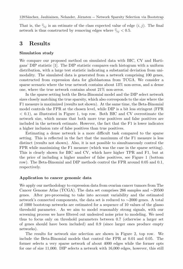
128Sanchez, Jauhiainen, Nelander, Jornsten -- Network Sparsity Selection via Bootstrap
That is, the γij is an estimate of the class expected value of edge (i, j). The finalnetwork is thus constructed by removing edges where γij < 0.5.
3 Results
Simulation study
We compare our proposed method on simulated data with BIC, CV and Harti-gans’ DIP statistic [1]. The DIP statistic compares each histogram with a uniformdistribution, with a large test statistic indicating a substantial deviation from uni-modality. The simulated data is generated from a network comprising 100 genes,constructed from expression data for glioblastoma from TCGA. We consider asparse scenario where the true network contains about 13% non-zeros, and a denseone, where the true network contains about 21% non-zeros.
In the sparse setting both the Beta-Binomial model and the DIP select networksizes closely matching the true sparsity, which also corresponds to the size where theF1 measure is maximized (results not shown). At the same time, the Beta-Binomialmodel controls the FPR at the chosen level, while DIP is a bit less stringent (FPR< 0.1), as illustrated in Figure 1, top row. Both BIC and CV overestimate thenetwork size, which means that both more true positives and false positives areincluded in the network estimate. However, the fact that the F1 is lower indicatesa higher inclusion rate of false positives than true positives.
Estimating a dense network is a more difficult task compared to the sparsesetting. This is reflected in the fact that the maximum of the F1 measure is lessdistinct (results not shown). Also, it is not possible to simultaneously control theFPR while maximizing the F1 measure (which was the case in the sparse setting).This is clearly shown for BIC and CV, which have higher TPR and F1, but atthe price of including a higher number of false positives, see Figure 1 (bottomrow). The Beta-Binomial and DIP methods control the FPR around 0.05 and 0.1,respectively.
Application to cancer genomic data
We apply our methodology to expression data from ovarian cancer tumors from TheCancer Genome Atlas (TCGA). The data set comprises 266 samples and ∼20500genes. After pre-processing to take into account variability and the estimatednetwork’s connected components, the data set is reduced to ∼2000 genes. A totalof 1000 bootstrap networks are estimated for a sequence of 10 values of the glassothreshold parameter. As we aim to model reasonably strong signals, with ourscreening process we have filtered out undesired noise prior to modeling. We needthus to focus only on threshold parameters between 0.7 (otherwise a larger setof genes should have been included) and 0.9 (since larger ones produce emptynetworks).
The results for network size selection are shown in Figure 2, top row. Weinclude the Beta-Binomial models that control the FPR at 0.01 and 0.05. Theformer selects a very sparse network of about 4000 edges while the former optsfor one of size 11,000. DIP selects a network with 16,000 edges, however, this still
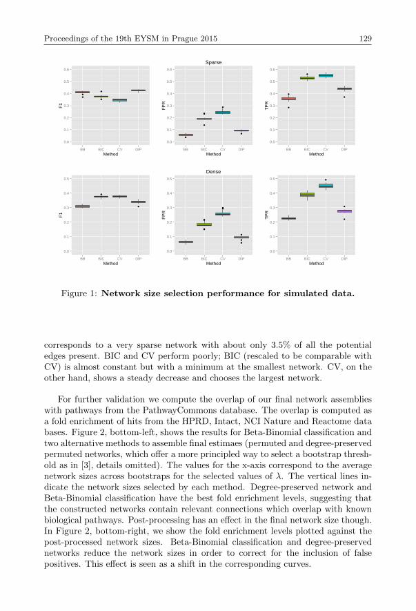
Proceedings of the 19th EYSM in Prague 2015 129
0.0
0.1
0.2
0.3
0.4
0.5
0.6
BB BIC CV DIPMethod
F1
0.0
0.1
0.2
0.3
0.4
0.5
0.6
BB BIC CV DIPMethod
FP
R
Sparse
0.0
0.1
0.2
0.3
0.4
0.5
0.6
BB BIC CV DIPMethod
TP
R
0.0
0.1
0.2
0.3
0.4
0.5
BB BIC CV DIPMethod
F1
0.0
0.1
0.2
0.3
0.4
0.5
BB BIC CV DIPMethod
FP
R
Dense
0.0
0.1
0.2
0.3
0.4
0.5
BB BIC CV DIPMethod
TP
R
Figure 1: Network size selection performance for simulated data.
corresponds to a very sparse network with about only 3.5% of all the potentialedges present. BIC and CV perform poorly; BIC (rescaled to be comparable withCV) is almost constant but with a minimum at the smallest network. CV, on theother hand, shows a steady decrease and chooses the largest network.
For further validation we compute the overlap of our final network assemblieswith pathways from the PathwayCommons database. The overlap is computed asa fold enrichment of hits from the HPRD, Intact, NCI Nature and Reactome databases. Figure 2, bottom-left, shows the results for Beta-Binomial classification andtwo alternative methods to assemble final estimaes (permuted and degree-preservedpermuted networks, which offer a more principled way to select a bootstrap thresh-old as in [3], details omitted). The values for the x-axis correspond to the averagenetwork sizes across bootstraps for the selected values of λ. The vertical lines in-dicate the network sizes selected by each method. Degree-preserved network andBeta-Binomial classification have the best fold enrichment levels, suggesting thatthe constructed networks contain relevant connections which overlap with knownbiological pathways. Post-processing has an effect in the final network size though.In Figure 2, bottom-right, we show the fold enrichment levels plotted against thepost-processed network sizes. Beta-Binomial classification and degree-preservednetworks reduce the network sizes in order to correct for the inclusion of falsepositives. This effect is seen as a shift in the corresponding curves.
130Sanchez, Jauhiainen, Nelander, Jornsten -- Network Sparsity Selection via Bootstrap
Figure 2: Network size selection performance for real data.
4 Future work
Our method can be used to select the tuning parameter for any network propertythat can be collected as a frequency statistic. Joint modeling of networks for groupsof samples belonging to different cancer types, can require fusing of edges (the edgevalues are estimated to be equal across classes). This problem can be solved byan extension of the graphical lasso, the so called fused graphical lasso ([4]), whichrequires tuning of a fusing parameter as well as a sparsity parameter. Fusing here,is an example of another network property for which frequency statistics can becollected. We plan to expand the applicability of our framework to include theselection of fusing parameters in the same principled way as selection of sparsityparameters.
Another line of work is to couple our framework to modularized networks, wherewe choose the sparsity level individually for the modular components. With thisapproach we control the false positive rate in each modular component separately,but while boosting the true positive rate in some modules with a higher signal-to-noise ratio. In this way, we also control the false positive rate globally, but allowingfor some modules to be denser (have more true positives) than what would beallowed with a global sparsity criterion.
Future work also includes a substantial decrease of computational burden byperforming a linesearch for a suitable sparsity threshold. The idea is to let the Beta-Binomial estimated parameters to guide the search aiming for a particular FPRcontrol, e.g. 0.01 and stop once it has been achieved. This approach improvesexecution time by reducing the number of threshold parameters for which thenetwork has to be estimated and by avoiding estimation of very dense networks.
Acknowledgements: The work presented here was supported by grants from theSwedish Research Council and Wallenberg Foundation.

Proceedings of the 19th EYSM in Prague 2015 131
References
[1] J. Hartigan, and P.M. Hartigan. The dip test of unimodality. The Annals ofStatistics, 70–84, 1985.
[2] R. Jornsten, T. Abenius, T. Kling, L. Schmidt, E. Johansson, T. Nordling, B.Nordlander, C. Sander, P. Gennemark, K. Funa, B. Nilsson, L. Lindahl, andS. Nelander. Network modeling of the transcriptional effects of copy numberaberrations in glioblastoma. Mol. Syst. Biol., 7(3):e33624, 2012.
[3] R. de Matos Simoes, and F. Emmert-Streib. Bagging statistical networkinference from large-scale gene expression data. PLoS ONE, 7:486, 2011.
[4] P. Danaher, and P. Wang, and D. Witten. The joint graphical lasso for inversecovariance estimation across multiple classes. Journal of the Royal StatisticalSociety: Series B (Statistical Methodology), 76(2): 373–397, 2014.

Adaptive Confidence Bands for Markov Chainsand Diffusions: Estimating the Invariant Measure
and the Drift
Jakob Sohl1 and Mathias Trabs∗2
1University of Cambridge, Statistical Laboratory, CB3 0WB, Cambridge, UK.2Humboldt-Universitat zu Berlin, Institut fur Mathematik, Unter den Linden 6,
D-10099 Berlin, Germany.
Abstract: As a starting point we prove a functional central limit theorem for es-timators of the invariant measure of a geometrically ergodic Harris-recurrent Mar-kov chain in a multi-scale space. Its proof is inspired by [2]. It allows to constructconfidence bands for the invariant density with optimal (up to undersmoothing)L∞-diameter by using wavelet projection estimators.
In addition our setting applies to the drift estimation for a diffusion
dXt = b(Xt)dt+ dWt, t ≥ 0,
observed discretely with fixed observation distance. We prove a functional centrallimit theorem for estimators of the drift function. Finally, adaptive confidencebands for the drift are constructed by using a data-driven estimator and based onthe ideas by [3]. Due to the Markovian structure of the observations, the proofsrely on a non-standard concentration inequality by [1].
Keywords: adaptive confidence bands, diffusion, drift estimation, ergodic Markovchain, functional central limit theorem
AMS subject classifications: 62G15, 60F05, 60J05, 60J60, 62M05
References
[1] R. Adamczak and W. Bednorz. Exponential concentration inequalities for addi-tive functionals of Markov chains. ESAIM. Probability and Statistics, to appear,2015.
[2] I. Castillo and R. Nickl. On the Bernstein–von Mises phenomenon for nonpara-metric Bayes procedures. The Annals of Statistics, 42(5):1941–1969, 2014.
[3] E. Gine and R. Nickl. Confidence bands in density estimation. The Annals ofStatistics, 38(2):1122–1170, 2010.
∗Corresponding author: [email protected]

The c -Loss Function: Balancing Total andIndividual Risk in the Simultaneous Estimation of
Poisson Means
Emil Aas Stoltenberg∗1 and Nils Lid Hjort1
1Department of Mathematics, University of Oslo, Norway
Abstract: This paper is devoted to the simultaneous estimation of the means of p ≥ 2independent Poisson distributions. A novel loss function that penalizes bad estimates ofeach of the means and the sum of the means is introduced. Under this loss function, aclass of minimax estimators that uniformly dominate the maximum likelihood estimator(MLE) is derived. Estimators in this class are shown to also be minimax and uniformlydominating under the commonly used weighted squared error loss function. Estimatorsin this class can be fine-tuned to limit shrinkage away from the MLE, thereby avoidingimplausible estimates of means anticipated to be bigger than the others. Further light isshed on this new class of estimators by showing that it can be derived by Bayesian andempirical Bayesian methods. Moreover, a class of prior distributions for which the Bayesestimators uniformly dominate the MLE under the new loss function is derived.
Keywords: Poisson, Bayes, simultaneous, estimation
AMS subject classifications: 60G09, 62G09
1 Introduction
Let Y = (Y1, . . . , Yp) be independent Poisson random variables with means θ =(θ1, . . . , θp), and let γ =
∑pi=1 θi. [1] showed that the MLE, δo(Y ) = Y (which is
also the uniformly minimum variance unbiased estimator), is inadmissible underthe weighted squared error loss function L1(δ, θ) =
∑pi=1 θ
−1i (δi − θi)2, provided
that p ≥ 2. [1] derived the estimator
δCZ(Y ) =
(1− p− 1
p− 1 + Z
)Y, (1)
where Z =∑pi=1 Yi, and showed that this estimator possesses uniformly smaller
risk than the MLE under L1.The estimator in (1), which “shrinks” the MLE towards the zero boundary of
the parameter space, guarantees a reduction in the total risk R(δ, θ) = EθL1(δ, θ)relative to the MLE. With regard to other objectives, however, it may performpoorly. First, it may yield implausible estimates of those θi with unusually highvalues. Second, it is likely to perform poorly in estimating the sum of the individ-ual Poisson means, γ. Recall that Z, the sum of p independent Poisson randomvariables, is itself Poisson with mean γ. In many situations where one is inter-ested in estimating an ensemble of Poisson means, one may also be interested in
∗Corresponding author: [email protected]

134 Stoltenberg and Hjort -- Simultaneous Estimation of Poisson Means
a good estimate of the sum of the means, or equivalently the mean of the means,θ = p−1γ. Think, for example, of a decision maker having to make budgetarydecisions concerning each of the boroughs of a city and the city as a whole.
The purpose of this paper is to develop a class of estimators that compromisebetween the Clevenson-Zidek estimator in (1) and the MLE. That is, a class ofestimators that has good ensemble properties with respect to the weighted squarederror loss function, and has good individual properties when it comes to estimatingthe individual θi and γ. The problem of shrinking the MLE towards non-zeropoints in the parameter space has been treated elsewhere, see e.g. [2].
2 The c -Loss function
Consider the following extension of the weighted squared error loss function,
Lc(δ, θ) =
p∑i=1
1
θi(δi − θi)2
+c
γ
(p∑i=1
δi − γ)2
. (2)
This loss function is equal to the weighted squared error loss function L1 plus anextra term that penalizes for bad estimates of γ, where the weight accorded to thisextra term is a function of the user-defined constant c. The risk of the MLE underLc is constant R(Y, θ) = p+ c.
We will now develop a class of estimators with uniformly smaller risk thanp + c. Consider estimators δ∗ = (δ∗1 , . . . , δ
∗p) of the form δ∗ = (1 − φ(Z))Y , where
Z =∑pi=1 Yi, Eθ|φ(Z)| <∞ and φ(z + 1)(z + 1) ≥ φ(z)z. Using that Eg(Y )/θ =
Eg(Y+1)/(Y+1) (for all integrable functions such that g(y) = 0, ∀ z ≤ 0), and thatconditional on Z the vector Y is multinomial with cell probabilities θi/γ, 1 ≤ i ≤ p,we obtain an expression for the difference in risk EθD = R(δ∗, θ)−R(Y, θ),
Eθ[Lc(δ∗, θ)− Lc(Y, θ)] = EθE[Lc(δ
∗, θ)− Lc(Y, θ)|Z]
= Eθ
(φ2(Z)− 2φ(Z))
Z[(p− 1) + (1 + c)Z]
γ+ 2(1 + c)φ(Z)Z
= Eθ
(φ2(Z + 1)− 2φ(Z + 1))[(p− 1) + (1 + c)(Z + 1)]
+ 2(1 + c)φ(Z)Z= EθDc(Z).
Here Dc is independent of the parameters, so a function φ(z) that ensures thatDc(z) ≤ 0 for all z with strict inequality for at least one datum z yields an estimatorthat uniformly dominates the MLE. A class of such functions is φ(z) = ψ(z)/(p−1 + (1 + c)z) where the function ψ is such that 0 < ψ(z) < 2(p − 1) and is non-decreasing for all z ≥ 0. This gives a class of estimators, denoted Dc, that uniformlydominate the MLE under (2), namely
δc(Y ) =
(1− ψ(Z)
p− 1 + (1 + c)Z
)Y. (3)
Theorem 31. For all θ ∈ Θ, estimators δc ∈ Dc have smaller risk than the MLEδo(Y ) = Y when loss is given by Lc in (2).

Proceedings of the 19th EYSM in Prague 2015 135
Proof. Use the expression for Dc above, then
R(δc, θ) = p+ c+ EγDc
= p+ c− 1
γEγ φ(Z)Z[2(p− 1 + (1 + c)(Z − γ))
− φ(Z)[p− 1 + (1 + c)Z]]
= p+ c− 1
γEγ φ(Z)Z[2(p− 1 + (1 + c)(Z − γ))− ψ(Z)]
≤ p+ c− 2
γEγ φ(Z)Z(1 + c)(Z − γ)
= p+ c− 2(1 + c)Eγ
[φ(Z)Z2
γ− φ(Z)Z
]= p+ c− 2(1 + c)Eγ [φ(Z + 1)(Z + 1)− φ(Z)Z]
≤ p+ c = R(Y, θ),
for all θ because φ(z)z is a strictly increasing function of z.
The optimal choice of ψ in terms of minimizing risk is p − 1. The estimatorin Dc with ψ(z) = p − 1 is denoted δc1. As seen from the proof above, the risk ofestimators in Dc depends on θi only through the sum γ, and is therefore easy tocompute numerically. The savings in risk relative to the MLE are substantial forsmall values of γ, and decrease as γ grows.
The difference in risk between estimators in Dc and the MLE under L1 isEγD(Z) = Eγ
(φ2(Z)− 2φ(Z))Z[(p− 1) + Z]γ−1 + 2φ(Z)Z
. Inserting this ex-
pression in the proof of Theorem 31 it is straightforward to show that estimatorsin Dc uniformly dominate the MLE under L1.
3 Bayes, minimax and admissibility
Let θ1, . . . , θp be independent and identically distributed (iid) Gamma randomvariables with mean a/b and variance a/b2 (denoted G(a, b)). The Bayes solutionunder the c -Loss function is then
δBj (y) =1 + c
1 + cg(z)
a+ yj − 1
b+ 1, (4)
where g(z) = (p(a− 1) + z)/(pa− 1 + z). With the prior sequence G(1, b/n)∞n=1
the minimum Bayes risk converges to p + c, i.e. the maximum risk of the MLE.This implies that the MLE is minimax under (2), hence (3) must also be minimax(see e.g. [5]).
In the following we sketch how estimators in the class Dc can be derived byBayesian methods in three different ways. First, the results of [3] in a L1-settingare extended to the c -Loss function. Let θi, 1 ≤ i ≤ p be iid G(1, b) and letb ∼ π2(b) ∝ bα−1 (b + 1)−(α+β). It can then be shown that the expectation ofθi given b and the data are as in (4) with b + 1 replaced by E[b + 1 |Z]. This

136 Stoltenberg and Hjort -- Simultaneous Estimation of Poisson Means
expectation is given by
E[b+ 1 |Z] =p+ α+ β + z − 1
z + β − 1.
Theorem 32. Assume that p > 2+c and consider the family of prior distributionsπ2(b) ∝ bα−1 (b+ 1)−(α+β) where
0 < α ≤ p− 2− c1 + c
and β > 0. Then the Bayes solution under the c -Loss function is a member of Dc.
Proof. Inserting the expression for E[b + 1 |Z] in the Bayes solution in (4) witha = 1 we obtain
δj(Y ) =(1 + c)(p− 1 + Z)
p− 1 + (1 + c)Z
z + β − 1
p+ α+ β + z − 1Yi. (5)
Recall that the estimators in Dc are of the form (1 − ψ(Z)/(p − 1 + (1 + c)Z))Yiwhere ψ is non-decreasing and 0 ≤ ψ(z) ≤ 2(p− 1) for all z. By some algebra weobtain that for the Bayes solution we here consider
ψ(z) = p− 1 + (1 + c)z − (1 + c)(p− 1 + z)z + β − 1
p+ α+ β + z − 1
= (1 + c)(p− 1 + z)(p+ α)
p− 1 + α+ β + z− c(p− 1).
This function is non-decreasing for all z ≥ 0. Moreover, we see that it is boundedabove by
supz≥0
ψ(z) = (1 + c)(p+ α) ≤ 2(p− 1),
since α ≤ (p− 2− c)/(1 + c). This means that the class of Bayes solutions in (5),where α satisfies the condition of the theorem, is in Dc.
Second, in an empirical Bayes setup the Poisson parameters are assumed iidG(1, b) and the parameter b is estimated from the data. An unbiased estimator ofb is z/(p− 1 + z). Inserting this estimator in (4) (and setting a = 1) we obtain theestimator δc1 given by
δc1(Y ) =
(1− p− 1
p− 1 + (1 + c)Z
)Y. (6)
This estimator is in Dc and, as mentioned, it is the optimal estimator in Dc interms of minimizing risk.
Finally, we show that the estimator δc1 in (6) can be derived as a generalizedBayes estimator. Reparametrize the Poisson means as θi = αiλ, 1 ≤ i ≤ p, andlet (α1, . . . , αp) be Dirichlet distributed with parameters (a1, . . . , ap). Define a0 =∑pi=1 ai. Let λ have the improper prior that is flat on the positive real line,
λ ∼ π(λ) ∝ I(λ > 0).

Proceedings of the 19th EYSM in Prague 2015 137
Using that Y |Z is multinomial the Poisson likelihood can be factorized as theproduct of a multinomial and the marginal of Z, this gives that the posteriordistribution θ1, . . . , θp is
π(θ1, . . . , θp |Y ) ∝ P (Y = y |Z)P (Z = z) Dirichlet(a1 . . . , ap)π(λ)
=z!
y1! · · · yp!αa1+y1−1
1 · · · αap+yp−1p λze−λ π(λ)
∝ Dirichlet(a1 + y1, . . . , ap + yp)G(z + 1, 1)π(λ),
(7)
which also shows that (α1, . . . , αp) and λ are independent. With this parametriza-tion the Bayes solution under the c -Loss function is
δBj (Y ) =1 + c
1 + cE[λ−1 |Y ]∑pi=1E[θ−1
i |Y ]−1E[θ−1
j |Y ]−1. (8)
With respect to the posterior distribution in (7), the expectation E[θ−1j |Y ] in
this expression is given by
E[θ−1j |Y ] =
∫ ∞0
∫S
1
αjλπ(θ1, . . . , θp |Y ) dα dλ
=
∫ ∞0
∫S
1
αjλ
Γ(a0 + z)∏pi=1 Γ(ai + yi)
p∏i=1
αai+yi−1i
G(z + 1, 1)π(λ) dα dλ
=
∫ 1
0
G(z + 1, 1)π(λ) dλ
∫S
αjΓ(a0 + z)∏pi=1 Γ(ai + yi)
p∏i=1
αai+yi−1i dα.
Here the expectation of αj over the simplex S is E[αj |Y ] = (a0+z−1)/(aj+yj−1).Inserting this in the posterior expectation of θ−1
j gives
E[θ−1j |Y ] =
a0 + z − 1
aj + yj − 1
∫ ∞0
1
λG(z + 1, 1)π(λ) dλ,
for j = 1, . . . , p. Morover, we have that
E[λ−1 |Z] =
∫ ∞0
1
λG(z + 1, 1)I(λ > 0) dλ =
1
z,
which gives
E[θ−1j |Y ] =
a0 + z − 1
aj + yj − 1
1
z.
In addition, the sum in (8) equals
p∑i=1
E[θ−1i |Y ]−1 = z
p∑i=1
aj + yj − 1
a0 + z − 1=
(a0 + z − p)za0 + z − 1
.
Now, let α1, . . . , αp be uniformly distributed over the simplex S. This is achievedby setting a1 = · · · = ap = 1. Then the sum a0 = p. In summary, with λ uniform

138 Stoltenberg and Hjort -- Simultaneous Estimation of Poisson Means
over R+ and the (α1, . . . , αp) uniform on the simplex S = [0, 1]p, the Bayes solutionunder the c -Loss function equals
δBj (Y ) =1 + c
1 + c 1Z
Z2
p−1+Z
Yjp− 1 + Z
=
(1− p− 1
p− 1 + (1 + c)Z
)Yj = δc1(Y ).
This means that in addition to being an empirical Bayes estimator, the new esti-mator δc1 is also a generalized Bayes estimator.
We have yet to find out whether the estimator δc1 in (6) is admissible. If we inthe prior distribution π2(b) ∝ bα−1 (b + 1)−(α+β) considered above set α = m − 1and β = 1, the estimator in (5) is admissible (since it is proper Bayes) for allm > 1. For m = 0 the estimator is equal to δc1, but it is then no longer properBayes. Thus, in a sense, we are “one unit” away from proving that the optimalestimator in terms of minimizing risk (under Lc) is admissible. See [6] for moredetails.
4 Conclusion
In this paper we have derived a class of minimax estimators that uniformly dom-inate the MLE under the c -Loss function in (2). Estimators in this class are alsominimax and uniformly dominant relative to the MLE under the weighted squarederror loss function L1. Importantly, estimators in this class can be fine-tuned inorder to achieve the desired amount of balancing between two conflicting desider-ata: good total risk and good individual risk in estimating individual θi and thesum γ.
References
[1] Clevenson, M.L. and J.V. Zidek Simultaneous Estimation of the Means ofIndependent Poisson Laws Journal of the American Statistical Association,70:698–705, 1975.
[2] Ghosh, M. and J.T. Hwang and K. Tsui Construction of Improved Estimatorsin Multiparameter Estimation for Discrete Exponential Families The Annalsof Statistics, 11:351–367, 1983.
[3] Ghosh, M. and A.Parsian Bayes Minimax Estimation of Multiple Poisson Pa-rameters Journal of Multivariate Analysis, 11:280–288, 1981.
[4] Peng, J. Simultaneous Estimation of the Parameters of Independent PoissonDisitributions Technical Report No. 48, Stanford University, Department ofStatistics, 1975
[5] Robert, C.P. The Bayesian Choice. From Decision-Theoretic Foundations toComputational Implementation. Springer, 2007.
[6] Stoltenberg, E. Aa. The c -Loss Function: Balancing Total and Individual Riskin the Simultaneous Estimation of Poisson Means Master’s thesis, Universityof Oslo, Department of Mathematics, 2015
Selection Consistency of Generalized InformationCriterion for Sparse Logistic Model
Hubert Szymanowski∗1 and Jan Mielniczuk12
1Institute of Computer Science Polish Academy of Sciences, Poland2Warsaw University of Technology, Poland
Abstract: We consider selection rule for small-n-large-P logistic regression whichconsists in choosing a subset of predictors minimizing Generalized Information Cri-terion over all subsets of variables of size not exceeding k. Consistency of such ruleunder weak conditions were established in [3]. This is a generalization of theresults of [2] to much broader regression scenario which allows also for a moregeneral criterion function than considered there and k depending on a sample size.We will discuss possibility of further weakening of the assumptions.
Keywords: consistency, information criterion, feature selection, sparse logisticregression
AMS subject classifications: 62J12, 62F07Acknowledgements: Study was supported by research fellowship within ”Infor-mation technologies: research and their interdisciplinary applications” (agreementnumber POKL.04.01.01-00-051/10-00)
References
[1] Chen J, and Chen Z. Extended Bayesian Information Criteria for model selec-tion with large model spaces. Biometrika, 95:759-771, 2008.
[2] Chen J., and Chen Z. Extended BIC for small-n-large-p sparse GLM. StatistSinica, 22:555-574, 2012.
[3] Mielniczuk J., and Szymanowski H. Selection consistency of Generalized In-formation Criterion for small-n-large-p sparse logistic model. In Springer Pro-ceedings in Mathematics & Statistics: Stochastic Models, Statistics and TheirApplications, Steland A., Rafaj lowicz E., Szajowski K., Eds., Vol. 122, 111-119,Springer, 2015.
∗Corresponding author: [email protected]
k-Sample Tests for Multivariate Censored Data
Mans Thulin∗
Department of Statistics, Uppsala University, Sweden
Abstract: The one-way MANOVA problem of testing whether the mean vectorsof several populations differ is common in many fields of research. In medicine,the rapid advance of high-throughput technologies has led to an increased interestin multivariate sets of biomarkers in e.g. blood samples. Such biomarkers canbe used to understand different diseases and how they are affected by treatmentsand covariates. Biomarker data is often left-censored because some measurementsfall below the laboratory’s detection limit. I will discuss how censoring affectsmultivariate two-sample and one-way MANOVA tests, in terms of size and power.Classical parametric tests are found to perform better than nonparametric alter-natives, which means that the current recommendations for analysis of censoredmultivariate data have to be revised. The good performance of the classical para-metric tests can at least partially be explained by some asymptotic results relatedto multivariate skewness and kurtosis. An expansion of the size of the classicaltests shows that up to o(n−1) the size is determined by skewness and kurtosis, andcloser inspection of the censoring process reveals that moderate censoring only hasa mild effect on these quantities. If the underlying distribution is approximatelynormal then moderate censoring will therefore not affect the size of the tests much.
Keywords: censored data, MANOVA, nondetects, two-sample test
AMS subject classifications: 62H15, 62F05, 62N03
∗Corresponding author: [email protected]

Forecasting Extreme Events in AgriculturalCommodity Markets
Athanasios Triantafyllou1, George Dotsis∗1 and Alexander H. Sarris1
1Department of Economics, University of Athens, Greece
Abstract: In this paper we empirically examine the predictive power of the riskneutral option-implied distribution on sudden (extreme) price spikes in agricul-tural commodity markets. We use as predictors of extreme returns the skewness ofthe risk neutral distribution, the variance risk premium and the tail risk measure.We find that our option-implied risk measures are robust and statistically signifi-cant predictors of the extreme events in the agricultural commodity markets. Ouroption-implied risk measures forecast both the magnitude and the probability ofoccurrence of a crash in these markets
Keywords: risk neutral moments, tail risk measures, extreme value theory, agri-cultural commodities
1 Introduction
In this paper we empirically estimate the forecasting power of the option-impliedrisk measures when used as predictors of extreme events in maize, wheat and soy-beans markets. With the term extreme event, we define what in the relevantliterature is called upward price spikes. While in the equity market the extremelyunlikely event is a sudden market crash, in agricultural markets the unlikely ex-treme event is defined as a sudden upward price spike, since sudden increases incommodity prices are most significant not only for commodity investors (at microlevel), but also for food security and policy issues in a macroeconomic level. Insimpler words, while the equity investors are fearful of the left tail of the distri-bution of returns, the commodity investors are fearful of the shape of right tail.Our option-implied measures are constructed using some results of Extreme ValueTheory (EVT) and of risk neutral valuation. Our primary motivations come fromthe literature in equity markets, in which the option-implied tail loss measuresadd significant forecasting power when used as predictors of stock-market crashes(Bollerslev et.al [3], Hamidieh [6], Vilkov et.al [8]). To the best of our knowledge,this is the first paper which deals with the forecasting of extreme events in agricul-tural commodity markets using option-implied information. While the empiricalworks in the relevant literature (e.g. Morgan et.al [7]) use the moments and the tailsof the physical distributions (the distribution of the realized returns in agriculturalcommodity markets) in order to forecast extreme upward spikes in these markets,we use the moments and the (right) tails of the risk neutral option-implied distribu-tion instead. Our contribution in the field is twofold: firstly, our empirical findings
∗Corresponding author: [email protected]
142 Triantafyllou, Dotsis and Sarris -- Forecasting Extreme Events
show that the option-implied information in agricultural markets is extremely use-ful, not only when forecasting the variance of agricultural prices (see Triantafyllouet.al [9], Wang, Fausti and Quasmi (2012)), but also when we forecast the suddenupward price movements. Our empirical findings implicitly reveal that the option-implied risk neutral distribution can (and must) be a risk management tool foragricultural commodity investors, since the risk management techniques are mostneeded and appreciated not in normal times, but in times of turbulence. By ourforecasting regressions, we find that our option-implied risk measures (namely riskneutral skewness, variance risk premia and Tail Risk Measures) add statisticallysignificant forecasting power when used as predictor of agricultural commodity re-turns. In addition, our option-implied risk measures contain all the forecastinginformation of the physical (realized) tail risk measure existed in the relevant liter-ature (Morgan et.al[7]). Secondly, when we define the extreme event in agriculturalmarkets as a 2 standard deviation rise (above the expected one) in monthly returns,our forecasting binary (probit) regressions show that our option-implied tail-riskmeasure captures and forecasts in a statistically significant manner these extremeprice spikes and the probability of the occurrence of these.
2 Methodology
2.1 Tail risk measure
In order to compute the tail risk measure we apply some results-tools of ExtremeValue Theory (EVT) on the risk neutral option-implied distribution. We applythe second theorem of EVT, known as the Pickands-Balkema-de Haan theorem,to describe the distribution of a commodity price X above an extreme (unusuallyhigh) threshold value h by a Generalized Pareto distribution of the form:
Gβ,ξ(h− x) =
l − (l + ξ h−xb )−
lξ ξ 6= 0
l − exp(−h−xb ) ξ = 0.(1)
The tail risk measure TLRh,t at time t given a specific pre-determined thresholdh is the expected excess tail value given in equation (2) relative to the current valuext, and it is the following formula:
E(h− x/h > x) =b
l − x (2)
The tail risk measure TLRh,t at time t given a specific pre-determined threshold his the expected excess tail value given in equation (2) relative to the current valuext, and it is the following formula:
TLRh,t =Et(h− x/h > x)
xt(3)
Under the risk neutral probability measure Q, we assume that the correspondingrisk neutral option-implied distribution belongs to the maximum domain of attrac-
Proceedings of the 19th EYSM in Prague 2015 143
tion of an extreme-value distribution Hξ. Then, the tail loss measure for a giventhreshold is unique1.
2.2 Model free option-implied moments
We compute the model-free version of option implied moments using the methodof Bakshi et.al. [1].Under the risk-neutral probability measure Q, the analyticalformulas for conditional risk neutral moments are given below:
V AR = Eqt (R2)− [Eqt (R)]2 (4)
SKEW =Eqt (R3)− 3Eqt (R)Eqt (R2) + [Eqt (R)]3
V AR3/2(5)
In accordance with Bakshi et.al. [1], we define the Quad and Cubic contracts2 asfollows:
Quad = exp(−r(T − t))Eqt (R2) (6)
Qubic = exp(−r(T − t))Eqt (R3) (7)
In the equations (6) and (7), r is the risk-free interest rate (3-month US-TreasuryBill), t is the trading date and T is the expiration date of a given contract and conse-quently T−t defines time to maturity. If we substitute Quad and Cubic expressionsgiven in equations (6) and (7) into equations (4) and (5), we get the model freeversion of option implied variance (MFIV ) and implied skewness (MFIS) givenbelow :
MFIV = exp(−r(T − t))Quad− [Eqt (R)]2 (8)
MFIS =exp(−r(T − t))Cubic− 3Eqt (R) exp(−r(T − t))Quad+ 2[Eqt (R)]3
MFIV 3/2(9)
Furthermore, Bakshi et.al [1] show that under the risk-neutral pricing measureQ, the Quad and Cubic contracts can be expressed as continuous functions ofout-of-the-money European calls C(t, T,K) and out-of-the-money European putsP (t, T,K) in the form given below:
Quad =
∫ ∞F
2(1− ln[KF ])
K2C(t, T,K)dK +
∫ F
0
2(1 + ln[ FK ])
K2P (t, T,K)dK (10)
Qubic =
∫ ∞F
6 ln[KF ]− 3 ln[KF ]2
K2C(t, T,K)dK−
∫ F
0
6 ln[ FK ] + 3 ln[ FK ]2
K2P (t, T,K)dK
(11)K is the strike price of the option contract, F is the price of the underlying futurescontract, t is the trading date and T is the expiration date of the option contract.
1See Vilkov et.al [8] for analytical proof of this proposition2If we define with R the logarithmic returns of the underlying asset with price St [R =
ln((St + 1ln(St)
)], then a Quad (or volatility) contract is a theoretical contract with risk neutral
quadratic expected return-payoff EQt (R2) and a Cubic contract is a contract with risk neutral
cubic expected return-payoff EQt (R3). Bakshi et.al. [1] prove that quadratic and cubic expected
risk neutral returns are continuous functions of Out of the Money (OTM) call and put optionprices.

144 Triantafyllou, Dotsis and Sarris -- Forecasting Extreme Events
In addition, Bakshi et.al. [1] prove that the expected (conditional on information attime t) risk-neutral returns Eqt (R) can be approximated by the following expression:
Eqt (R) = exp(r(T − t))− 1− exp(r(T − t))2
Quad− exp(r(T − t))6
Qubic (12)
Knowing the analytical forms of Quad and Cubic contracts from equations (6) andeqrefQubic, and the approximating quantity of conditional risk neutral expectedreturns Eqt (R) from equation (12), we can compute by using numerical integrationthe model free option-implied moments given in equations (8) and (9).
2.3 Variance risk premium
The variance risk premium represents the compensation demanded by investors forbearing variance risk and it is defined as the difference between realized varianceand a risk-neutral model-free implied variance (MFIVt). According to Bliss et.al[2] and Carr et.al [4] is a reliable measure of risk aversion in financial markets.More specifically, following Carr et.al [4] and Christoffersen et.al [5], we define thevariance risk premium as the difference between the P−measure expected varianceand the Qmeasure expected variance, using the following formula:
V RP (t, T ) = EPt (RV (t, T ))− EQt (RV (t, T )) (13)
References
[1] Bakshi, G., Kapadia, N. & D. Madan (2003). Stock Return Characteristics,Skew Laws, and the Differential Pricing of Individual Equity Options, Reviewof Financial Studies,15,101-143.
[2] Bliss, R. R. & N. Panigirtzoglou (2004). Option-Implied Risk Aversion Esti-mates.Journal of Finance,LIX,407-446.
[3] Bollerslev, T. & G. Todorov (2011). Tails, Fears and Variance Risk Premia,Journal of Finance,66,2165-2211.
[4] Carr, P. & L. Wu (2009). Variance Risk Premiums. Review of Financial Stud-ies,22,1311-1341.
[5] Christoffersen, P., Kang, S. B. & Pan, X. (2010). Does Variance Risk PremiumPredicts Futures Returns? Evidence in the Crude Oil Market. Working Paper
[6] Hamidieh, K. (2011). Recovering the Tail Shape Parameter of the Risk NeutralDensity from Option Prices. Working paper
[7] Morgan, W., Cotter, J. & K. Dowd (2012). Extreme Measures of AgriculturalFinancial Risk. Journal of Agricultural Economics, 63,65-82.
[8] Vilkov, G. & Y. Xiao (2013). Option-Implied Information and Predictability ofExtreme Returns. SAFE Working Paper 5

Proceedings of the 19th EYSM in Prague 2015 145
[9] Triantafyllou, A., Dotsis, G & A.H. Sarris (2015). Volatility Forecasting andTime-Varying Variance Risk Premia in Grains Commodity Markets. Journal ofAgricultural Economics, (forthcoming)

Overview of Some Interesting Statistical Problemsin Biochemical Analysis of Glycans
Ivo Ugrina∗
University of Zagreb, Croatia
Abstract: Glycomics is rapidly emerging field in high-throughput biology thataims to systematically study glycan structures of a given protein, cell type ororganic system. As within other high-throughput methods in biology (microarrays,metabolomics, proteomics), accuracy of high-throughput methods is highly affectedby complicated experimental procedures leading to differences between replicatesand the existence of batch effects, among others. Study of appropriate methodsfor normalization, appropriate designs of experiments and batch removal methodstailored to the needs of glycomics is therefore a necessity.
Keywords: batch effects, normalization, noise, glycomics
AMS subject classifications: 62P10, 92C40
1 Introduction
Glycans are important structural and functional components of the majority ofproteins. However, their structural complexity and the absence of a direct genetictemplate impedes understanding of the role of glycans in biological processes. Arecent comprehensive report endorsed by the US National Academies concludedthat glycans are directly involved in the pathophysiology of every major diseaseand that additional knowledge from glycoscience will be needed to realize the goalsof personalized medicine [11].
This conclusion gave importance to the already existing field of biochemicalanalysis of glycans. Currently, numerous studies in the development of biochemicalanalysis of glycans are conducted. Successful implementation of high-throughputanalytical techniques for glycan analysis resulted in publication of GWAS of thehuman glycome [9, 7, 8, 6]. A number of studies have investigated the role ofglycans in human disease, including autoimmune diseases and cancer [2, 10].
Biochemical analysis of glycans is usually conducted with one of the followingmethods: UPLC-FLR, ultraperformance liquid chromatography with fluorescencedetection; CGE-LIF, multiplex capillary gel electrophoresis with laser induced flu-orescence detection; MALDI-TOF-MS, matrix assisted laser desorption/ionizationtime of flight MS; LC-ESI-MS, liquid chromatography electrospray MS.
Complexity of these methods, together with the complexity of glycans usuallyleads to different effects like batch effects or multiplicative errors making subsequentanalysis of results more cumbersome. Therefore, the need for greater expertise instatistical and computer science methods becomes obvious.
∗Corresponding author: [email protected]

Proceedings of the 19th EYSM in Prague 2015 147
GP
1
GP
2
GP
3G
P4
GP
5G
P6
GP
7G
P8
GP
9
GP
10
GP
11
GP
12
GP
13
GP
14
GP
15
GP
16
GP
17
GP
18
GP
19
GP
20
GP
21G
P22
GP
23G
P24
GP
25
GP
26
GP
27G
P28
GP
29
GP
30
GP
31G
P32
GP
33G
P34
GP
35
GP
36
GP
37
GP
38
GP
39
0
50
100
5 10 15 20Time (min)
Inte
nsity
(E
U)
Figure 1: An example of a chromatogram from the UPLC analysis of glycan com-position from the blood plasma sample.
2 Problems
Especially problematic is the multiplicative error as a consequence of laboratoryconditions and the current practice of removing that error. An example of a resultfrom the biochemical analysis of glycans with UPLC method from blood plasma isgiven in Figure 1. This is an example of a chromatogram. If one denotes the areasunder the chromatogram between appropriate borders with GP∗ the graph can berepresented as a random vector GP = (GP1, . . . , GP39). Multiplicative error thenmeans that for every run of the biochemical analysis the results will be of the formGP = C · GP where C denotes a random variable. Therefore, every run will givedifferent intensities.
Current methodology within the filed of glycomics approaches the problem ofthe multiplicative error by the usage of Total Area Normalization. Normalizationrefers to the creation of shifted and scaled versions of statistics, where the intentionis that these normalized values allow the comparison of corresponding normalizedvalues for different datasets. Total Area Normalization (TAN), also called percent-age normalization, is given by the transformation
GPTANi =GPi∑j GPj
.
Although this normalization procedure works fine for the basic quality controlit introduces many problems like spurious correlations (making network/pathwayanalysis problematic) or other problems with the constrained data (see [12, 1] formore details).
Another big problem in the analysis of glycans is the existence of batch effectssimilarly to the fields of metabolomics or microarray experiments. Conducting aglycan analysis on a big population means that the analysis will almost always be

148 Ugrina -- Statistical Analysis of Glycomics Data
10
15
20
2 4 6Batch
Inte
nsity
Figure 2: An example of batch effects (differences in medians and spread) withinthe UPLC analysis of blood plasma samples presented with boxplots.
conducted in batches of 100 to 1000 samples. As the time between the analysis ofbatches increases the probability of the introduction of some random effect increasesalso. This could be due to the changes on the machine where the analysis isconducted or by the change of a lab analyst.
Unfortunately, the current practice in glycomics research often ignores the prob-lem of batch effects and therefore increases the probability of false results in latterstatistical analysis.
An example of batch effects on an experiment designed to infer the experimentalvariability is given in Figure 2. Since all batches consist of the same (replicated)samples the results should behave the same. However, the batches were prepared bydifferent lab analysts at different time points introducing batch effects non-intrinsicto the underlying samples.
Appropriate design of experiments is also sometimes ignored by the currentpractice in the field of biochemical analysis of glycans. This is closely connectedwith the aforementioned existence of batch effects since the prerequisite for batchcorrection procedures is an effective design of the experiment.
3 Improvements
The current practice can be improved by the introduction of appropriate methodsfor the design of experiments like randomized block designs [3], exploration of theeffects of other normalization procedures like quantile normalization or mediannormalization [4] and the introduction of batch correction techniques like linearmixed effect models and empirical Bayes methods [5].
Acknowledgements: This research was supported by EU projects: MIMOmics(contract #305280) and IntegraLife (contract #315997).

Proceedings of the 19th EYSM in Prague 2015 149
References
[1] Wiley: Compositional Data Analysis: Theory and Applications - VeraPawlowsky-Glahn, Antonella Buccianti.
[2] B. Adamczyk, T. Tharmalingam, and P. M. Rudd. Glycans as cancer biomark-ers. Biochimica Et Biophysica Acta, 1820(9):1347–1353, Sept. 2012.
[3] S. Addelman. The Generalized Randomized Block Design. The AmericanStatistician, 23(4):35–36, Oct. 1969.
[4] B. M. Bolstad, R. A. Irizarry, M. Astrand, and T. P. Speed. A comparisonof normalization methods for high density oligonucleotide array data basedon variance and bias. Bioinformatics (Oxford, England), 19(2):185–193, Jan.2003.
[5] C. Chen, K. Grennan, J. Badner, D. Zhang, E. Gershon, L. Jin, and C. Liu.Removing Batch Effects in Analysis of Expression Microarray Data: An Eval-uation of Six Batch Adjustment Methods. PLoS ONE, 6(2):e17238, Feb. 2011.
[6] J. E. Huffman, A. Knezevic, V. Vitart, J. Kattla, B. Adamczyk, M. Novokmet,W. Igl, M. Pucic, L. Zgaga, . Johannson, I. Redzic, O. Gornik, T. Zemunik,O. Polasek, I. Kolcic, M. Pehlic, C. A. M. Koeleman, S. Campbell, S. H. Wild,N. D. Hastie, H. Campbell, U. Gyllensten, M. Wuhrer, J. F. Wilson, C. Hay-ward, I. Rudan, P. M. Rudd, A. F. Wright, and G. Lauc. Polymorphismsin B3gat1, SLC9a9 and MGAT5 are associated with variation within the hu-man plasma N-glycome of 3533 European adults. Human Molecular Genetics,20(24):5000–5011, Dec. 2011.
[7] Z. Kutalik, B. Benyamin, S. Bergmann, V. Mooser, G. Waeber, G. W. Mont-gomery, N. G. Martin, P. A. F. Madden, A. C. Heath, J. S. Beckmann, P. Vol-lenweider, P. Marques-Vidal, and J. B. Whitfield. Genome-wide associationstudy identifies two loci strongly affecting transferrin glycosylation. HumanMolecular Genetics, 20(18):3710–3717, Sept. 2011.
[8] G. Lauc, A. Essafi, J. E. Huffman, C. Hayward, A. Kneevi, J. J. Kattla,O. Polaek, O. Gornik, V. Vitart, J. L. Abrahams, M. Pui, M. Novokmet,I. Redi, S. Campbell, S. H. Wild, F. Boroveki, W. Wang, I. Koli, L. Zgaga,U. Gyllensten, J. F. Wilson, A. F. Wright, N. D. Hastie, H. Campbell, P. M.Rudd, and I. Rudan. Genomics Meets GlycomicsThe First GWAS Study ofHuman N-Glycome Identifies HNF1 as a Master Regulator of Plasma ProteinFucosylation. PLoS Genet, 6(12):e1001256, Dec. 2010.
[9] G. Lauc, J. E. Huffman, M. Pui, L. Zgaga, B. Adamczyk, A. Muini, M. Novok-met, O. Polaek, O. Gornik, J. Kriti, T. Keser, V. Vitart, B. Scheijen, H.-W.Uh, M. Molokhia, A. L. Patrick, P. McKeigue, I. Koli, I. K. Luki, O. Swann,F. N. van Leeuwen, L. R. Ruhaak, J. J. Houwing-Duistermaat, P. E. Slagboom,M. Beekman, A. J. M. de Craen, A. M. Deelder, Q. Zeng, W. Wang, N. D.Hastie, U. Gyllensten, J. F. Wilson, M. Wuhrer, A. F. Wright, P. M. Rudd,C. Hayward, Y. Aulchenko, H. Campbell, and I. Rudan. Loci Associated with

150 Ugrina -- Statistical Analysis of Glycomics Data
N-Glycosylation of Human Immunoglobulin G Show Pleiotropy with Autoim-mune Diseases and Haematological Cancers. PLoS Genet, 9(1):e1003225, Jan.2013.
[10] Y. Mechref, Y. Hu, A. Garcia, and A. Hussein. Identifying cancer biomark-ers by mass spectrometry-based glycomics. Electrophoresis, 33(12):1755–1767,July 2012.
[11] National Research Council (US) Committee on Assessing the Importanceand Impact of Glycomics and Glycosciences. Transforming Glycoscience: ARoadmap for the Future. The National Academies Collection: Reports fundedby National Institutes of Health. National Academies Press (US), Washington(DC), 2012.
[12] R. Pincus. Aitchison, J.: The Statistical Analysis of Compositional Data.Chapman and Hall, London - New York 1986, XII, 416 pp., 25,00. BiometricalJournal, 30(7):794–794, Jan. 1988.

The Horseshoe and More General Sparsity Priors
Stephanie L. van der Pas∗
Leiden University, Netherlands
Abstract: We study the sparse normal means problem, where the mean vectoris sparse in the nearly black sense. Adopting the frequentist framework where thedata is generated according to some fixed mean vector, we use the posterior meanresulting from the horseshoe prior to recover the mean vector. We show that theposterior rate of convergence is at most of the order of the minimax rate. Thehorseshoe prior is not unique in this regard, as some recent extensions of the workon the horseshoe prior show.
Keywords: horseshoe, sparsity, Bayesian inference, normal means problem
AMS subject classifications: 62F15
1 Introduction
A common test case for sparsity methods is the sparse normal means problem,where we observe a vector Y n ∈ Rn, Y n = (Y1, . . . , Yn), such that
Yi = θi + εi, i = 1, . . . , n,
for independent standard normal random variables εi. The vector θ = (θ1, . . . , θn)is the vector of interest, and is assumed to be sparse in the nearly black sense,meaning that the number of nonzero entries of θ,
pn := #i : θi 6= 0
is o(n) as n→∞. Our goal is to recover θ, and to provide uncertainty quantifica-tion.
We focus in this paper on Bayesian methods. Thus, we use the posterior distri-bution to achieve both of our goals. The typical choice for our goal of recovery isto use a measure of centre, such as a median, mean, or mode as an estimator. Foruncertainty quantification, a credible set is a natural object to use from a Bayesianpoint of view. To achieve realistic uncertainty quantification, the posterior shouldcontract to its center at the same rate at which the estimator approaches the trueparameter.
A well-studied approach has been to induce sparsity through a spike and slabprior [6], which is a mixture of a Dirac measure at zero (to account for the zeromeans) and a continuous distribution (to account for the nonzero means). Anempirical Bayes version of this approach, where the mixing weight is obtained
∗Corresponding author: [email protected]

152 Van der Pas -- The Horseshoe and More General Sparsity Priors
through marginal maximum likelihood, was found to work well for recovery [5], butno measure of uncertainty quantification was studied. For a fully Bayesian version,several combinations of priors on the mixing weight and on the nonzero coefficients(the ‘slab’) were found such that both goals are achieved [2]. Unfortunately, a spikeand slab approach runs into computational difficulties, as it may require explorationof a model space of size 2n.
Therefore, there is a need for priors that are not only suitable for recovery anduncertainty quantification, but are also feasible computationally on large data sets.The horseshoe prior is one such prior. In this paper, we review the theoreticalresults for the horseshoe prior, as described in [7]. The work has recently beenextended in [4], and in forthcoming joint work with J. Schmidt-Hieber and J.-B.Salomond, which will be discussed during the presentation, and briefly in Section4. We first review the horseshoe prior in Section 2, then discuss some posteriorcontraction results from [7] for the horseshoe prior in Section 3.
2 The horseshoe prior
The horseshoe prior was introduced by [1] and has the following hierarchical for-mulation:
θi | λi, τ ∼ N (0, τ2λ2i ), λi ∼ C+(0, 1),
for i = 1, . . . , n, where C+(0, 1) is a standard half-Cauchy distribution. We use thecoordinatewise posterior mean Tτ (yi) as our estimator of θi. Figure 1 shows theprior density on each θi, and the posterior mean as a function of the observationyi. It illustrates the role of the global parameter τ : decreasing τ leads to moremass near zero in the prior on θi and a stronger shrinkage effect in the posteriormean Tτ (y).
Figure 1: (Based on Figure 1 in [7]) The effect of decreasing τ on the prior on θ(left) and the posterior mean Tτ (y) (right). The solid line corresponds to τ = 1,the dashed line to τ = 0.05. Decreasing τ results in a higher prior probability ofshrinking the observations towards zero.
The parameter τ controls the sparsity, and results from [7] show that the optimalchoice for τ is the proportion of nonzero means pn/n (up to a log factor). The role

Proceedings of the 19th EYSM in Prague 2015 153
of the parameters λi is to counteract the shrinkage effect at a local level.The horseshoe estimator offers a computational advantage over the spike-and-
slab approach, as it can be expressed as follows:
Tτ (yi) = yi
∫ 1
0z1/2 1
τ2+(1−τ2)z ey2i /2dz∫ 1
0z−1/2 1
τ2+(1−τ2)z ey2i /2dz
.
In case τ is estimated empirically, the posterior mean can be computed by pluggingthis estimate into the above expression, circumventing the need to use MCMC. Itcan be evaluated via a quadrature routine, or by a representation in terms ofconfluent hypergeometric functions, as discussed in [8].
3 Posterior contraction results for the horseshoe
In this section, some posterior contraction results from [7] are discussed. The mainresult is Theorem 33, which provides upper bounds on the rate of contraction ofthe posterior distribution around the true mean vector, and around the posteriormean. Denote the class of nearly black vectors by `0[pn] = θ ∈ Rn : #i : θi 6=0 ≤ pn.
Theorem 33 (Theorem 3.3 in [7]). Suppose Y n ∼ N (θ0, In), n, pn → ∞, pn =o(n) and τ = (pn/n)α, α ≥ 1. Then:
supθ0∈`0[pn]
Eθ0Πτ
(θ : ‖θ − θ0‖2 > Mnpn log
n
pn
∣∣∣Y n )→ 0,
and
supθ0∈`0[pn]
Eθ0Πτ
(θ : ‖θ − Tτ (Y n)‖2 > Mnpn log
n
pn
∣∣∣Y n )→ 0,
for any Mn →∞.
These upper bounds are equal, up to a multiplicative constant, to the minimaxrisk [3]. The contraction rate around the true mean vector θ0 is therefore sharp,but this is not necessarily the case for the rate of contraction around the posteriormean Tτ (Y n).
Further investigation into the role of τ (Theorems 3.4 and 3.5 of [7]) shows thatif τ = (pn/n)α for α ∈ (0, 1), the posterior variance may exceed the minimax rate,indicating suboptimal spread of the posterior. If α > 1, there exists a sequenceθ0,n ∈ `0[pn] for which the mean square error and the posterior variance are ofdifferent orders. If α = 1, the posterior variance and `2 risk only differ by a factor√
log(n/pn), and the gap can even be closed by taking τ = (pn/n)√
log(n/pn).Thus, for our goals of recovery and uncertainty quantification, the best choice
for τ is τ = (pn/n)√
log(n/pn), as in that case both the worst case `2 risk and theposterior variance are at the order of the minimax risk (Theorems 3.1, 3.2 and 3.4in [7]).
In practice, the number of nonzero means pn is typically unknown, and hencethe value τ = (pn/n)
√log(n/pn) cannot be used. However, an empirical Bayes
154 Van der Pas -- The Horseshoe and More General Sparsity Priors
procedure, in which τ is estimated from the data, can still yield the (near) minimaxrate for the worst case risk. For example, consider for any c1 > 2, c2 > 1, theestimator
τ = max
#|yi| ≥
√c1 log n, i = 1, . . . , n
c2n,
1
n
.
This estimator estimates the number of nonzero means by counting those observa-tions that are past the universal threshold
√2 log n. It is bounded below by 1/n for
computational reasons, and because it corresponds to the assumption that there isat least one nonzero mean. By Theorem 4.1 combined with Lemma A.7 from [7],the horseshoe estimator combined with this estimator of τ will have a worst caserisk of order pn log n, which is close to the minimax rate unless the truth is notvery sparse.
4 Other sparsity priors
In [4], priors of the form
θi | λ2i , τ
2 ∼ N (0, λ2i τ
2), λ2i ∼ π(λ2
i ), i = 1, . . . , n
are considered, for priors π with density given by
π(λ2i ) = K
1
(λ2i )a+1
L(λ2i ),
whereK > 0 is a constant and L : (0,∞)→ (0,∞) is a non-constant, slowly varyingfunction, where ‘slowly varying’ means that there exist c0,M ∈ (0,∞) such thatL(t) > c0) for all t ≥ t0 and supt∈(0,∞) L(t) ≤ M . The horseshoe is containedin this class of priors, by taking a = 1/2, L(t) = t/(1 + t) and K = 1/π. Theauthors prove a posterior contraction theorem of the same type as Theorem 33 forthis class of priors, provided α ∈ [1/2, 1]. Although their results for lower boundson the posterior variance are limited to the case a = 1/2, their results extendthose for the horseshoe, showing that the horseshoe is not unique in its desirableposterior concentration properties. Forthcoming work with J. Schmidt-Hieber andJ.-B. Salomond provides some more general conditions on sparsity priors such thatthe posterior concentrates at least as fast as the minimax rate.
Acknowledgements: Research supported by Netherlands Organization for Sci-entific Research NWO. This paper is based on joint work with Aad van der Vaart,Bas Kleijn, Johannes Schmidt-Hieber and Jean-Bernard Salomond.
References
[1] C. M. Carvalho, N. G. Polson and J. G. Scott. The horseshoe estimator forsparse signals. Biometrika, 97(2):465-480, 2010.
[2] I. Castillo and A. W. van der Vaart. Needles and straw in a haystack: pos-terior concentration for possibly sparse sequences. The Annals of Statistics,40(4):2069–2101, 2012.

Proceedings of the 19th EYSM in Prague 2015 155
[3] D. L. Donoho, I. M. Johnstone, J. C. Hoch and A. S. Stern. Maximum entropyand the nearly black object (with discussion). Journal of the Royal StatisticalSociety. Series B (Methodological), 54:41–81, 1992.
[4] P. Ghosh and A. Chakrabarti. Posterior concentration properties of a generalclass of shrinkage estimators around nearly black vectors. arXiv:1412.8161,2013.
[5] I. M. Johnstone and B. W. Silverman. Needles and straw in haystacks: em-pirical Bayes estimates of possibly sparse sequences. The Annals of Statistics,32(4):1594–169, 2004.
[6] T. J. Mitchell and J. J. Beauchamp. Bayesian variable selection in linear re-gression. Journal of the American Statistical Association, 83(404):1023–1032,1988.
[7] S. L. van der Pas, B. J. K. Kleijn and A. W. van der Vaart. The horseshoe esti-mator: posterior concentration around nearly black vectors. Electronic Journalof Statistics, 8:2585–2618, 2014.
[8] N. G. Polson and J. G. Scott. Good, great, or lucky? Screening for firmswith sustained superior performance using heavy-tailed priors. The Annals ofApplied Statistics, 6:161–185, 2012.
Goodness-Of-Fit Tests for Exponentiality Basedon Yanev-Chakraborty Characterization and
Their Efficiencies
Ksenia Volkova∗
Saint-Petersburg State University, Russia
Abstract: Two scale-free goodness-of-fit tests for exponentiality based on therecent characterization of exponential law by Yanev and Chakraborty are pro-posed. Test statistics are functionals of U -empirical processes. The first of thesestatistics is of integral type, it is similar to the classical statistics ω1
n. The secondone is a Kolmogorov type statistic. The limiting distribution and large deviationsasymptotic of new statistics under null hypothesis are described. Their local Ba-hadur efficiency for parametric alternatives is calculated. The Kolmogorov typestatistic is not asymptotically normal, therefore we evaluate the critical values byusing Monte-Carlo methods. For small sample size efficiencies are compared withsimulated powers of new tests. Also conditions of local asymptotic optimality ofnew statistics in the sense of Bahadur are discussed and examples of such specialalternatives are given.
Keywords: testing of exponentiality, order statistics, U -statistics, Bahadur effi-ciency
AMS subject classifications: 60F10, 62G10, 62G20, 62G30
1 Introduction
We develop goodness-of-fit tests for exponentiality exploiting a characterizationbased on property of order statistics. The problem formulation is as follows: letX1, X2, . . . , Xn be i.i.d. observations having the continuous df F . Consider testingof composite hypothesis of exponentiality H0 : F ∈ E(λ), where E(λ) denotes theclass of exponential distributions with the density f(x) = λe−λx, x ≥ 0, whereλ > 0 is some unknown parameter.
Suppose that the df F belongs to the class of distributions F , if the correspond-ing density f has derivatives of all orders in the neighbourhood of zero.
Arnold and Villasenor in [1] conjectured, and Yanev and Chakraborty in [8]proved that the following characterized the exponential law within the class F :
Let X1, . . . , Xn be non-negative i.i.d. rv’s with df F from class F . Then thestatistics max(X1, X2, X3) and max(X1, X2) + X3
3 are identically distributed if andonly if the df F is exponential.
∗Corresponding author: [email protected]

Proceedings of the 19th EYSM in Prague 2015 157
Consider the usual empirical df Fn(t) = n−1∑ni=1 1Xi < t, t ∈ R1, based on
the observations X1, . . . , Xn. According to the characterization we construct fort ≥ 0 the U -empirical df’s by the formulae
Hn(t) =
(n
3
)−1 ∑1≤i1<i2<i3≤n
1max(Xi1 , Xi2 , Xi3) < t, t ≥ 0,
Gn(t) =1
3
(n
3
)−1 ∑1≤i1<i2<i3≤n
[1max(Xi1 , Xi2) +Xi3
3< t+
+ 1max(Xi2 , Xi3) +Xi1
3< t+ 1max(Xi3 , Xi1) +
Xi2
3< t], t ≥ 0.
It is known that the properties of U -empirical df’s are similar to the propertiesof usual empirical df’s, see [2]. Hence for large n the df’s Hn and Gn should beclose under H0, and we can measure their closeness by using some test statistics.
We suggest two scale-invariant statistics
In =
∫ ∞0
(Hn(t)−Gn(t)) dFn(t), (1)
Dn = supt≥0| Hn(t)−Gn(t) |, (2)
assuming that their large values are critical.
2 Integral statistic In
Without loss of generalization we can assume that λ = 1. The statistic In isasymptotically equivalent to the U -statistic of degree 4 with the centered kernelΨ(X1, X2, X3, X4) given by
Ψ(X1, X2, X3, X4) =1
4
∑π(i1,...,i4)
1max(Xi1 , Xi2 , Xi3) < Xi4−
− 1
24
∑π(i1,...,i4)
1max(Xi1 , Xi2) +Xi3
3< Xi4,
where π(i1, . . . , i4) means all permutations of different indices from i1, . . . , i4.Theorem 34. Under null hypothesis as n → ∞ the statistic In is asymptoticallynormal with asymptotic variance given by
√nIn
d−→ N (0,23
10920).
2.1 Large deviations of the statistic In
The kernel Ψ is centered, bounded and non-degenerate. Hence according to thetheorem of large deviations for such statistics from [5], we obtain the followingresult.

158 Volkova -- Goodness-Of-Fit Tests for Exponentiality and Their Efficiencies
Theorem 35. For a > 0
limn→∞
n−1 lnP (In > a) ∼ 5460
23a2, as a→ 0.
3 Kolmogorov-type statistic Dn
Now we consider the Kolmogorov type statistic (2). Its indisputable merit is con-sistency against any alternative that follows directly from the characterization assuch, while the integral statistic In is not always consistent.
In our case for fixed t ≥ 0 the difference Hn(t)−Gn(t) is a family of U -statisticswith the kernels, depending on t ≥ 0 :
Ξ(X,Y, Z; t) = 1max(X,Y, Z) < t − 1
31max(X,Y ) +
Z
3< t−
−1
31max(Y,Z) +
X
3< t − 1
31max(X,Z) +
Y
3< t.
Limiting distribution of the statistic Dn is unknown. Using the methods of [6],one can show that the U -empirical process
ηn(t) =√n (Hn(t)−Gn(t)) , t ≥ 0,
weakly converges in D(0,∞) as n → ∞ to certain centered Gaussian process η(t)with calculable covariance. Then the sequence of statistics
√nDn converges in
distribution to the rv supt≥0 |η(t)| but it is impossible to find explicitly its distri-bution. Hence it is reasonable to determine the critical values for statistics Dn bysimulation.
3.1 Large deviations of the statistic Dn
The family of kernels Ξ(X,Y, Z; t), t ≥ 0 is not only centered but bounded. Usingthe results from [4] on large deviations for the supremum families of non-degenerateU -statistics, we obtain the following result.
Theorem 36. For a > 0
limn→∞
n−1 lnP (Dn > a) ∼ 4.966a2, as a→ 0.
4 Local Bahadur efficiencies of statistics In and Dn
We present the following alternatives against exponentiality which will be consid-ered for all tests when x ≥ 0:
i) Makeham distribution with the density g1(x, θ) =(1 + θ(1 − e−x)
)exp
(−
x− θ(e−x − 1 + x)), θ > 0;
ii) Weibull distribution with the density g2(x, θ) = (1 + θ)xθ exp(−x1+θ), θ > 0;

Proceedings of the 19th EYSM in Prague 2015 159
iii) gamma distribution with the density g3(x, θ) = xθ
Γ(θ+1)e−x, θ > 0;
iv) exponential mixture with negative weights (EMNW(β)) (see [3]) g4(x) =
(1 + θ)e−x − θβe−βx, θ ∈[0, 1
β−1
], β > 1.
We calculate the efficiencies of both statistics against common alternatives fromthe class F . The statistic Dn has the non-normal limiting distribution, hence weuse the Bahadur approach as a method of calculation of asymptotic efficiency,while the classical Pitman approach to efficiency is not applicable. However, it isknown that the local Bahadur efficiency and the limiting Pitman efficiency usuallycoincide, see [7]. Finally, we analyze the conditions of local asymptotic optimalityof our tests and describe the ”most favorable” alternatives for them.
We supplement our research with simulated powers which principally supportthe theoretical values of efficiency.
Acknowledgements: The research of the author was supported by the grantsRFBR 13-01-00172, NSh. 2504.2014.1, and SPbGU 6.38.672.2013.
References
[1] B. C. Arnold, J. A. Villasenor. Exponential characterizations motivated by thestructure of order statistics in samples of size two. Statistical and ProbabilityLetters, 83:596–601, 2013.
[2] R. Helmers, P. Janssen, R. Serfling. Glivenko-Cantelli properties of some gener-alized empirical DF’s and strong convergence of generalized L-statistics. Prob-ability Theory and Related Fields, 79:75–93, 1988.
[3] V. Jevremovic. A note on mixed exponential distribution with negative weights.Statistical and Probability Letters, 11(3):259–265, 1991. doi: 10.1016/0167-7152(91)90153-I.
[4] Ya. Yu. Nikitin. Large deviations of U -empirical Kolmogorov-Smirnov tests,and their efficiency. Journal of Nonparametric Statistics, 22:649–668, 2010.
[5] Ya. Yu. Nikitin, E. V. Ponikarov. Rough large deviation asymptotics of Cher-noff type for von Mises functionals and U -statistics. Proceedings of the St.Petersburg Mathematical Society, 7:124–167, 1999. English translation in AMSTranslations, 2(203):107–146, 2001.
[6] B. W. Silverman. Convergence of a class of empirical distribution functions ofdependent random variables. The Annals of Probability, 11:745–751, 1983.
[7] H. S. Wieand. A condition under which the Pitman and Bahadur approaches toefficiency coincide. The Annals of Mathematical Statistics, 4:1003–1011, 1976.
[8] G. P. Yanev, S. Chakraborty. Characterizations of exponential distributionbased on sample of size three. Pliska Studia Mathematica Bulgarica, 23:237-244, 2013.

Simultaneous Perturbation GradientApproximation Based Metropolis AdjustedLangevin Markov Chain Monte Carlo for
Inference of Ordinary Differential Equations
Ivan Vujacic∗1 and Mathisca de Gunst1
1VU University Amsterdam, Netherlands
Abstract: The problem of parameter estimation for models defined by a systemof ordinary differential equations (ODEs) is considered. The most efficient way toexplore the parameter space is by using derivative information. Usual approachesfor obtaining the gradient in ODEs setting like solving sensitivity equations andusing finite difference formulas are computationally costly and not scalable to largescale systems. In this paper we use simultaneous perturbation gradient approxi-mation (SPGA), originally proposed in stochastic optimization literature, as a sub-stitute for the gradient in Metropolis adjusted Langevin algorithm (MALA). Theobtained algorithm, called Simultaneous Perturbation Gradient Approximation ba-sed Metropolis Adjusted Langevin Markov chain Monte Carlo (SPGA MALA), re-quires at most three integration of the ODE system per MCMC step, regardless ofthe dimension of the system. This fixed computational costs makes SPGA MALAapplicable to large scale systems. On the other hand, its efficiency is comparableto that of MALA. We demonstrate the performance of via simulations.
Keywords: Metropolis adjusted Langevin Markov Chain Monte Carlo methods,simultaneous perturbation gradient approximation, ordinary differential equations,parameter estimation
AMS subject classifications: 60J22, 65C40, 62F15
1 Introduction
Systems of ordinary differential equations (ODEs) are widely used in science andengineering for the mathematical modelling of various dynamic processes. Weconsider the system of the form
x′(t) = f(x(t), t;θ), t ∈ [0, T ],x(0) = ξ,
(1)
where x(t) = (x1(t), . . . , xd(t))> ∈ Rd is a state vector, ξ in Ξ ⊂ Rd is the initial
condition, θ in Θ ⊂ Rp is a parameter and f is a known function. Given thevalues of ξ and θ, we denote the solution of (1) by x(t;θ, ξ). Let us assume thata process is modelled by the system (1) with ξ0 known and θ0 unknown. For
∗Corresponding author: [email protected]

Proceedings of the 19th EYSM in Prague 2015 161
simplicity, assume that we have noisy observations yi(tj), j = 1, . . . , n of all thestates xi(t;θ0, ξ0), i = 1, . . . , d at time points tj ∈ [0, T ], j = 1, . . . , n:
yi(tj) = xi(tj ;θ0, ξ0) + εi(tj), i = 1, . . . , d; j = 1, . . . , n,
where εi(tj) ∼ N (0, σ2i ). The problem is to estimate θ0 from the data Y =
(yi(tj))ij . The methodology presented here can also be used if ξ0 is unknown andsome of the states are unobserved.
In this paper, we adopt Bayesian approach to inference. For some prior densityπ of θ the posterior density is
p(θ|Y, ξ0,σ) = π(θ)
d∏j=1
NYj,·|X(θ, ξ0)j,·, σjIn,
where σ = (σ1, . . . , σd), X(θ, ξ0) = (xi(tj ;θ, ξ0))ij and In is an identity matrix oforder n. For exploring the parameter space there is an advantage in using gradientinformation in MCMC and optimization methods [3, 4]; for concrete examples inODE estimation setting see [4, 6]. In the problem we consider, the gradient of thelog-likelihood can be obtained by solving sensitivity equations, which are of orderdp or via the finite difference formulas, which require solving the ODE system atleast p times. Both approaches are computationally costly and not scalable to largescale systems.
In this paper, we avoid huge computational burden by using simultaneous per-turbation stochastic approximation (SPGA), introduced by Spall [7]. To obtainSPGA, the system of the form (1) need be solved at most 2 times, regardless ofthe dimension of the system. By using SPGA instead of the gradient in Metropo-lis adjusted Langevin Markov Chain Monte Carlo (MALA) we obtain a method,which we call SPGA MALA, that can be used for large scale systems. Althoughthere is some loss in efficiency of SPGA MALA due to using an approximation ofthe derivative this is outweighed by huge computational savings achieved.
The rest of the paper is organized as follows. In sections 2 and 3 reviews ofMALA and SPGA are provided, respectively. Section 4 introduces the proposedmethod. In Section 5 we compare performance of MALA and SPGA MALA onsimulated data for various models.
2 Metropolis adjusted Langevin Markov chainMonte Carlo (MALA)
For the probability density p(θ) let L(θ) = logp(θ) denote the log-density. TheMALA proposal [4, p.130] is
θ∗ = θk + ε2M∇θL(θk)/2 + ε√
Mzk, (2)
where θk is the value at k-th step, z ∼ N (z|0, Ip), ε > 0 is the step size and M isthe weight matrix. The proposal density and acceptance probability are
q(θ∗|θk) = N (θ∗|µ(θk, ε), ε2M),α = min1, p(θ∗)q(θk|θ∗)/p(θk)q(θ∗|θk), (3)

162 Vujacic and De Gunst -- SPGA MALA
respectively, where µ(θk, ε) = θk + ε2M∇θL(θk)/2. The advantage of MALA overrandom walk Metropolis algorithm is that it uses the gradient information whichleads to better exploration of the parameter space. Disadvantage is that it requiresselection of the weight matrix M. In [4], a fully automated algorithm is proposedfor this but it cannot be used in our setting because it requires derivatives. Formore details regarding MALA see [2, 4].
3 Simultaneous perturbation gradient approxima-tion (SPGA)
In order to estimate partial derivatives via finite difference (FD) approximation theparameter perturbations are performed along each coordinate separately. For ex-ample, the estimate of the j-th partial derivative of L(θk) via the central differenceformula is
∂L(θk)
∂θj≈ L(θk + hej)− L(θk − hej)
2h,
where ej is the j-th unit vector and h is sufficiently small. This requires 2p eval-uations of L. With simultaneous perturbation (SP), introduced by Spall [7], allelements of θk are randomly perturbed together. The two sided simultaneous per-turbation gradient approximation (SPGA) is
∇θL(θk) =L(θk + h∆)− L(θk − h∆)
2h(∆−1
1 ,∆−12 , . . . ,∆−1
p )>, (4)
where ∆ = (∆1,∆2, . . . ,∆p)> is usually a random vector of independent Bernoulli
random variables that take values −1 and 1 with probability 0.5, although otherchoices are possible. Two sided SPGA requires two evaluations of L regardlessof the dimension p. FD approximation is superior to SP approximation as anestimator of the gradient. However, Spall [7] showed that when used in stochas-tic optimization setting they achieve the same level of statistical accuracy for agiven number of iterations in terms of estimation of the optimum of the objectivefunction. In the next section, we follow the same idea but in the MCMC setting.
4 Simultaneous perturbation gradient approxima-tion based Metropolis adjusted Langevin Mar-kov chain Monte Carlo (SPGA MALA)
SPGA MALA proposal is obtained by substituting the gradient in MALA proposal(2) with its SPGA, defined in (4):
θ∗ = θk + ε2M∇θL(θk)/2 + ε√
Mzk. (5)
In view of the MALA proposal density in (3), we require that the density of θ∗
given θk and ∆ is q(θ∗|θk,∆) = N (θ∗|µ(θk, ε,∆), ε2M), where µ(θk, ε,∆) = θk +
ε2M∇θL(θk)/2. Since ∆ can take 2p values with equal probability it follows that

Proceedings of the 19th EYSM in Prague 2015 163
the density of θ∗ given θk is the mixture density q(θ∗|θk) = 12p
∑∆ q(θ∗|θk,∆).
The proposal mechanism (5) with proposal density q and standard accepetanceprobability α = min1, p(θ∗)q(θk|θ∗)/p(θk)q(θ∗|θk) defines a valid Markov chain;it is simply Metropolis Hastings (MH) algorithm where the proposal is a mixturedensity q. However, evaluating α is intractable for large p. Because of this, insteadof α we use
α∆ = min1, p(θ∗)q(θk|θ∗,∆)/p(θk)q(θ∗|θk,∆).
In other words, instead of using q which involves calculation of each q(θ∗|θk,∆)for 2p possible values of ∆, we use the acceptance ratio which involves calculationof q(θ∗|θk,∆) only for the drawn value of ∆.This algorithm defines a valid Markov chain since it can be viewed as Metropolis-Hastings-Green(MHG) algorithm [2, p.41]. MHG algorithm allows state-dependentmixing or random proposals [1], meaning that on each step the proposal distributionneed not be fixed but can belong to a countable family of proposal distributions.In our case it is a finite family q(θ∗|θk,∆) : ∆ = (∆1, . . . ,∆p),∆i ∈ −1, 1.Using the random proposal instead of the mixture proposal comes with a price. Aspointed out in the discussion section of the article [1], the random proposal methodis less efficient because it accepts fewer proposals. This reduces efficiency of SPGAMALA. The second reason for reduced efficiency of SPGA MALA is that insteadof the gradient its approximation is used. However, it is clear that SPGA MALAwill be much faster than MALA for large scale systems.
5 Numerical results
In this section we compare the described algorithm to MALA on simulated datagenerated from the following models.Fitz Hugh Nagumo (FHN) example. Fitz-Hugh Nagumo system [4] modelsthe behaviour of spike potentials in the giant axon of squid neurons. It has theform
x′1(t) = θ3x1(t)− x1(t)3/3 + x2(t),x′2(t) = − 1
θ3x1(t)− θ1 + θ2x2(t).
We used different notation than in [4], namely (x1, x2) for (V,R) and (θ1, θ2, θ3)for (a, b, c). We set θ = (0.2, 0.2, 3) and ξ = (−1, 1).α- pinene example. The following model describes the thermal isomerization ofα-pinene [8].
x′1(t) = −(θ1 + θ2)x1(t),x′2(t) = θ1x1(t),x′3(t) = θ2x1(t)− (θ3 + θ4)x3(t) + θ5x5(t),x′4(t) = θ3x3(t),x′5(t) = θ4x3(t)− θ5x5(t).
The values of the parameters that we used are θ = (0.1, 0.1, 0.3, 0.1, 0.3) and ξ =(1, 0, 0, 0, 0).Hockin model. In [5], a model of the extrinsic blood coagulation is developedand consists of 34 differential equations and 42 rate constants. Due to lack of space

164 Vujacic and De Gunst -- SPGA MALA
we do not present the model but refer the reader to the aforementioned reference.We fixed 32 parameters and estimated the remaining 10. The value of the selectedparameter was set to θ = (0.1, 0.4, 0.1, 0.32, 0.2, 1.05, 2.4, 6, 1.8, 8.2).
From each of the models presented above we generated 200 data points on theinterval [0, 20] and added Gaussian-distributed noise with standard deviation equalto 0.5. In SPGA (see (4)) we set h = 10e−5 while the gradient in MALA is obtainedby solving sensitivity equations. Ideally, the tuning parameters in MALA shouldbe chosen in such a way that acceptance rate is between 40% and 70%. As it waspointed out in Section 2, tuning of MALA is an issue. To simplify, for both MALAand SPGA MALA we set M = Ip, ε = 0.0002p−1/3 in all the simulations. Thisselection achieves the desired acceptance rate in FHN model and was used in [4].For the other two models this is not the case. However, the most important thinghere is to compare the performance of these two methods for the same selection oftuning parameters. For comparing sampling efficiency we followed approach usedin [4]. A single Markov chain was initialized on the true mode and 5000 posteriorsamples were collected. The effective sample size (ESS) for each parameter wascalculated; the minimum of ESS was used to calculate the time per effectivelyindependent sample. For each method we ran 10 simulations, using the same dataset. The methods were implemented in the interpreted language MATLAB and allcomputations were carried out on an Intel Core i5 computer with 1.3 GHz processorspeed and 4 GB of memory. The results of our simulations are presented in Table 1.
The results of FHN example demonstrate loss in efficiency of SPGA MALA withrespect to MALA; see Section 4 for the discussion. In α-pinene example MALA isstill faster even though the sensitivity equations are of order 25. This is becausethe original system and the system of sensitivity equations are both linear. The ex-ample of Hockin model show the advantage of SPGA MALA. Sensitivity equationsare of order 340 and this heavily affects the computatation time of MALA. On theother hand, the computation time of SPGA MALA is much smaller compared tothat of MALA, making it much better in terms of the relative speed per effectivelyindependent sample.
Acknowledgements: This research is supported by the Dutch Technology Foun-dation STW, which is part of the Netherlands Organisation for Scientific Research(NWO), and which is partly funded by Ministry of Economic Affairs. Mark Giro-lami and Ben Calderhead are acknowledged for making their MATLAB code used in[4] freely available. We thank Itai Dattner and Bart Bakker for useful comments.
References
[1] J. Besag, P. Green, D. Higdon, and K. Mengersen. Bayesian computation andstochastic systems. Statistical science, pages 3–41, 1995.
[2] S. Brooks, A. Gelman, G. Jones, and X.-L. Meng. Handbook of Markov ChainMonte Carlo. CRC press, 2011.
[3] A. R. Conn, K. Scheinberg, and L. N. Vicente. Introduction to derivative-freeoptimization, volume 8. Siam, 2009.
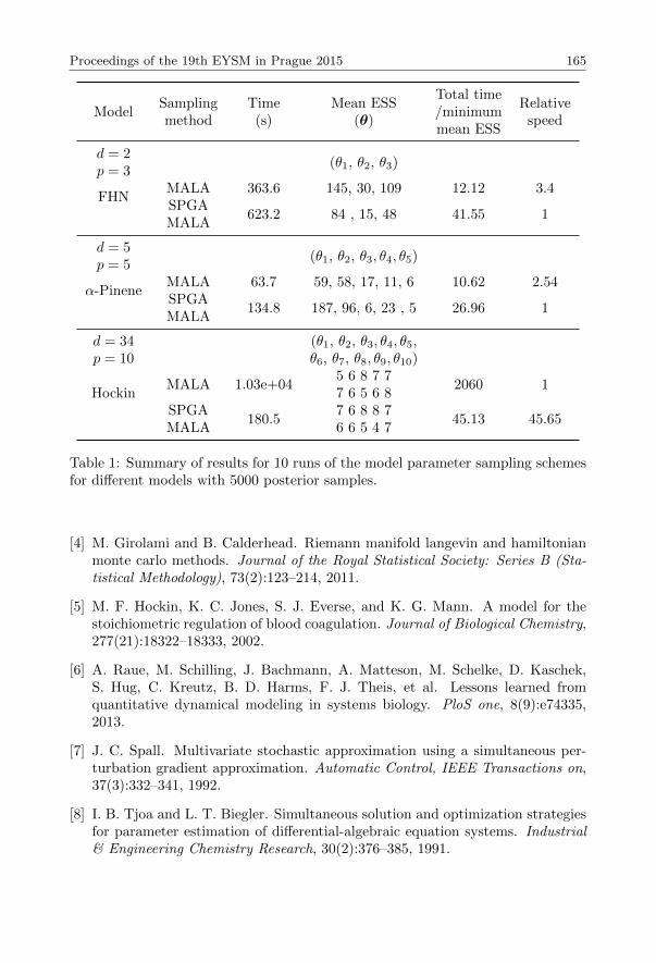
Proceedings of the 19th EYSM in Prague 2015 165
ModelSamplingmethod
Time(s)
Mean ESS(θ)
Total time/minimummean ESS
Relativespeed
d = 2p = 3
(θ1, θ2, θ3)
FHNMALA 363.6 145, 30, 109 12.12 3.4SPGAMALA
623.2 84 , 15, 48 41.55 1
d = 5p = 5
(θ1, θ2, θ3, θ4, θ5)
α-PineneMALA 63.7 59, 58, 17, 11, 6 10.62 2.54SPGAMALA
134.8 187, 96, 6, 23 , 5 26.96 1
d = 34p = 10
(θ1, θ2, θ3, θ4, θ5,θ6, θ7, θ8, θ9, θ10)
HockinMALA 1.03e+04
5 6 8 7 77 6 5 6 8
2060 1
SPGAMALA
180.57 6 8 8 76 6 5 4 7
45.13 45.65
Table 1: Summary of results for 10 runs of the model parameter sampling schemesfor different models with 5000 posterior samples.
[4] M. Girolami and B. Calderhead. Riemann manifold langevin and hamiltonianmonte carlo methods. Journal of the Royal Statistical Society: Series B (Sta-tistical Methodology), 73(2):123–214, 2011.
[5] M. F. Hockin, K. C. Jones, S. J. Everse, and K. G. Mann. A model for thestoichiometric regulation of blood coagulation. Journal of Biological Chemistry,277(21):18322–18333, 2002.
[6] A. Raue, M. Schilling, J. Bachmann, A. Matteson, M. Schelke, D. Kaschek,S. Hug, C. Kreutz, B. D. Harms, F. J. Theis, et al. Lessons learned fromquantitative dynamical modeling in systems biology. PloS one, 8(9):e74335,2013.
[7] J. C. Spall. Multivariate stochastic approximation using a simultaneous per-turbation gradient approximation. Automatic Control, IEEE Transactions on,37(3):332–341, 1992.
[8] I. B. Tjoa and L. T. Biegler. Simultaneous solution and optimization strategiesfor parameter estimation of differential-algebraic equation systems. Industrial& Engineering Chemistry Research, 30(2):376–385, 1991.

Author Index
Ozkul, Eda, 113
Amghar, Mohamed, 1
Angelov, Slav, 7
Arpino, Bruno, 24
Askin, Oykum Esra, 8
Bancescu, Irina Adriana, 9
Biolan, Bogdan Corneliu, 10
Blazere, Melanie, 12
Brzyski, Damian, 18
Burclova, Katarına, 22
Cannas, Massimo, 24
Claeskens, Gerda, 56
Cribben, Ivor, 30
Cuevas, Antonio, 31
de Gunst, Mathisca, 160
Dotsis, George, 141
Dvorak, Jirı, 34
Fazekas, Istvan, 117
Fiecas, Mark, 40
Gamboa, Fabrice, 12
Ganychenko, Iurii, 45
Godichon, Antoine, 50
Gueuning, Thomas, 56
Heiny, Johannes, 62
Hjort, Nils Lid, 133
Inan, Deniz, 8
Jornsten, Rebecka, 125
Jakubık, Jozef, 64
Jankova, Jana, 69
Jansen, Maarten, 1
Jauhiainen, Alexandra, 125
Kormendi, Kristof, 81
Kesemen, Orhan, 113
Kley, Tobias, 70
Koleva, Dessislava, 76
Kozachenko, Yuriy, 100
Kulik, Alexei, 45
Llop, Pamela, 31
Loubes, Jean-Michel, 12
Markeviciute, Jurgita, 82
Mielniczuk, Jan, 139
Miettinen, Jari, 88
Mikkelsen, Frederik Riis, 94
Mikosch, Thomas, 62
Milev, Mariyan, 76
Mlavets, Yuriy, 100
Navratil, Radim, 106
Nelander, Sven, 125
Nordhausen, Klaus, 88
Noszaly, Csaba, 117
Oja, Hannu, 88
Ombao, Hernando, 40
Pazman, Andrej, 22
Pap, Gyula, 81
Papatsouma, Ioanna, 115
Pateiro-Lopez, Beatriz, 31
Perecsenyi, Attila, 117
Porvazsnyik, Bettina, 117
Preinerstorfer, David, 118
Rossi, Maurizia, 119
Sohl, Jakob, 132
Sanchez, Jose, 125
Sarris, Alexander H., 141
166

Proceedings of the 19th EYSM in Prague 2015 167
Stoltenberg, Emil Aas, 133
Szymanowski, Hubert, 139
Taskinen, Sara, 88
Thulin, Mans, 140
Trabs, Mathias, 132
Triantafyllou, Athanasios, 141
Ugrina, Ivo, 146
van der Pas, Stephanie L., 151
van de Geer, Sara, 69
Volkova, Ksenia, 156
Vujacic, Ivan, 160
Yu, Yi, 30