procedural analysis of choice rules with applications to ... · were listed on american’s...

American Economic Review 101 (April 2011): 724–748http://www.aeaweb.org/articles.php?doi=10.1257/aer.101.2.724

724

In 1981, an internal study by American Airlines found that travel agents booked the first flight that appeared on their computer screen 53 percent of the time, and a flight that appeared somewhere on the first screen almost 92 percent of the time. This provided an incentive for American to manipulate the order in which flights were listed on American’s “Sabre” computer reservation system, which domi-nated the market for electronic flight booking. Allegations by smaller airlines that American—and United Airlines which owned the second largest computer reserva-tion system “Apollo”—engaged in such manipulations led the US federal govern-ment to regulate screen display in computer reservation systems.1

This example, in which the order of the alternatives affects decision making, is by no means unique. In elections, for example, being listed first on the ballot increases the likelihood of winning office, mainly at the expense of candidates listed in the middle of the ballot.2 In competitions, judges tend to award higher

1 See US Department of Justice (1983), US General Accounting Office (1986), and Duncan G. Copeland, Richard O. Mason, and James L. McKenney (1995).

2 Joanne M. Miller and Jon A. Krosnick (1998) and Krosnick, Miller, and Michael P. Tichy (2004) find statistically significant and sometimes substantively large effects of being listed first on the vote shares of major party candidates in US federal elections. Jonathan G. S. Koppell and Jennifer A. Steen (2004) and Daniel E. Ho and Kosuke Imai (2008) find similar effects for major party candidates in primary elections in the United States. Amy King and Andrew Leigh (2008) replicate these findings in partisan Australian federal elections. Marc Meredith and Salant (2009) find that in local elections in California, the proportion of election winners from the first ballot position is larger than expected and the proportion of winners from the median ballot position is smaller than expected, absent order effects.

Procedural Analysis of Choice Rules with Applications to Bounded Rationality

By Yuval Salant*

I study how limited abilities to process information affect choice behav-ior. I model the decision-making process by an automaton, and mea-sure the complexity of a specific choice rule by the minimal number of states an automaton implementing the rule uses to process informa-tion. I establish that any choice rule that is less complicated than utility maximization displays framing effects. I then prove that choice rules that result from an optimal trade-off between maximizing utility and minimizing complexity are history-dependent satisficing procedures that display primacy and recency effects. (JEL D01, D03, D11, D83)

* Kellogg School of Management, Northwestern University, 2001 Sheridan Rd, Evanston, IL (e-mail: [email protected]). I am indebted to Bob Wilson for his devoted guidance, constant support, and most valuable sug-gestions. I am grateful to Ariel Rubinstein and Jeremy Bulow for the encouragement, productive discussions, and important comments. I thank Gil Kalai, Ron Siegel, and Andy Skrzypacz for most insightful feedback in various stages of this project. I also thank Drew Fudenberg, Jon Levin, Michael Ostrovsky, Roy Radner, Ilya Segal, and seminar participants at UC Berkeley, Brown University, Caltech, Harvard University, Hebrew University, University of Iowa, LSE, MIT, Northwestern University, NYU, Stanford University, Tel-Aviv University, UCL, Washington University in St. Louis, and Yale University for helpful comments. This research is supported in part by the Leonard W. and Shirley R. Ely Fellowship of the Stanford Institute for Economic Policy Research.

725SALAnt: PRocEduRAL AnALySISVoL. 101 no. 2

scores to contestants who appear later in the competition.3 And in designing a menu, restaurant managers are advised to position their highest profit-margin items first, second,and last on the menu.4 In these and other contexts, investigating the sources and nature of order effects may provide a deeper understanding of their economic, strategic, and policy consequences.

One of the sources of order effects is likely to be cognitive and procedural limita-tions.5 Choosing the best available flight, for example, seems cognitively demanding because it may involve comparing each flight to every other flight. Travel agents may find it simpler to choose the first satisfactory flight that appears on their screen. Similarly, recalling the performance of the last contestant in a competition seems simpler than recalling the performances of those who appeared before him, which may lead to a tendency to choose the last contestant.

The goal of this paper is to investigate how certain cognitive and procedural limi-tations relate to order effects and choice behavior. The main takeaway from the analysis is that any choice rule that is procedurally simpler than utility maximiza-tion displays order effects, and that primacy and recency effects as well as other common behavioral effects emerge when an expected utility maximizer optimally economizes on procedural costs.

In the procedural model I investigate, the decision maker can be in one of several states. A state may reflect the state of mind of the decision maker. For example, a satisficer, who chooses the first satisfactory alternative he encounters, is “unsatis-ficed” until he encounters a satisfactory alternative and becomes “satisficed.” A state may also capture information the decision maker considers relevant for making a choice. For example, when maximizing a utility function, a state may record the best alternative encountered so far.

States are used in processing information and making choices. The decision maker encounters the alternatives in a form of a list (as in the examples above), and processes them one after the other as follows. He starts in some predetermined state. When considering the next alternative in the list, he decides (as a function of his cur-rent state and the current alternative) whether to stop and make a choice or continue. If the decision maker continues, he updates his state as necessary and then considers the next alternative. When reaching the last alternative, the decision maker must make a choice, if he has not yet done so. For example, a satisficer may be thought of as staying in the “unsatisficed” state until he encounters a satisfactory alternative, in which case he stops and chooses it.

States are costly in the sense that the more states a decision maker uses in making choices, the more cognitive resources he expends and the finer the information he utilizes. The state complexity of a given choice behavior is the minimal number of states needed to implement that behavior.

3 Order effects have been found in contests such as the World Figure Skating Competition (Wändi Bruine de Bruin 2005), the International Synchronized Swimming Competition (Vietta E. Wilson 1977), the Eurovision Song Contest (Bruine de Bruin 2005), and the Queen Elisabeth Contest for violin and piano (Herbert Glejser and Bruno Heyndels 2001).

4 See Jack E. Miller (1980).5 In a seminal work, Herbert A. Simon (1955) argued that cognitive and procedural considerations may push

decision makers toward various forms of “boundedly” rational behavior, and suggested satisificing as an alternative to utility maximization. The bounded rationality literature develops this idea in different contexts.

726 tHE AMERIcAn EconoMIc REVIEW APRIL 2011

State complexity was used to measure the complexity of strategies in repeated games and the complexity of decision rules in the context of individual inference making.6 It reflects the cognitive costs associated with refining the information used in making decisions. It is also related to the notion of categorization, as I show in Section III. Intuitively, the decision maker may be thought of as classifying past information into one of several categories, each of which corresponds to a state, and then processing future information based on this classification.

Clearly, the complexity of making choices involves additional procedural aspects beyond those captured by state complexity. For example, it may be costly for a deci-sion maker to understand which alternatives are feasible, or to search for the next alternative. In analyzing the effect of state complexity on choice behavior, I make only a first step in understanding the effects of cognitive and procedural limitations on individual choice behavior.

I focus on comparing the state complexity of utility maximization, or rational choice, to that of other behaviors. A rational decision maker has in mind a strict preference relation ≻ over the alternatives that he maximizes when making choices.7 Rational choice is frequently used in economics to model the behavior of economic agents and is robust to order effects.

The way a rational decision maker processes information depends on the identity of the best alternative he encountered so far. For every two alternatives x and y, the set of alternatives that are ≻-superior to x is different from the set of alternatives that are ≻-superior to y, and therefore a rational decision maker needs two different states to account for how future information will be processed conditional on see-ing x and conditional on seeing y. This implies that the state complexity of rational choice nearly equals the number of feasible alternatives.8 Satisficing is much simpler in terms of state complexity since the only relevant information in processing the next available alternative is whether a satisfactory alternative has already appeared.

The first main result of the paper is that utility maximization is procedurally sim-plest among all choice rules that are robust to order effects.9 That is, rational choice is uniquely simplest among all choice rules that are order-independent, i.e, rules that choose the same alternative from every two lists that are permutations of one another. In addition, rational choice is simplest among all choice rules that are order-independent for lists with just two alternatives, but possibly order-dependent for larger lists. Put another way, any choice rule that is simpler than rational choice is order-dependent. This result provides a possible procedural explanation for why we

6 Abraham Neyman (1985), Ariel Rubinstein (1986), Dilip Abreu and Rubinstein (1988), and others study state complexity in the context of repeated games. James Dow (1991) and Andrea Wilson (2002) study state complexity in the context of inference making.

7 A strict preference relation is a complete, asymmetric, and transitive binary relation.8 No state is required for processing information conditional on seeing the ≻-maximal alternative, because in that

case the decision maker can stop and choose the ≻-maximal alternative.9 Several papers have pointed out that rational choice is “simple.” Donald E. Campbell (1978) and Taradas

Bandyopadhyay (1988) show that intuitive procedural properties characterize choice correspondences that can be represented as the maximization of a binary relation. Rubinstein (1996) suggests that the frequent appearance of order relations in natural language can partly be explained by the fact that order relations are easy to describe. Gil Kalai (2003) shows that rational behavior is easy to learn in the Probably-Approximately-Correct learning model. Michael Mandler (forthcoming) shows that in a model of choosing by a checklist of criteria, rational agents make choices faster than nonrational agents.


see order effects in real-life decision making: by using the order, decision makers are able to simplify the complexity of making choices.

As mentioned above, the state complexity of rational choice nearly equals the number of feasible alternatives. Hence, when the number of alternatives is large, rational choice becomes cognitively demanding. For example, when choosing among flights the number of possible choices may be very large and processing every two flights differently may be complicated. In such a case, a decision maker may replace utility maximization with a choice rule that is “close” to utility maxi-mization but uses fewer states. One possibility is to satisfice or perhaps fully rank-order only a few flights and compare all other flights to these “pivotal” flights. I investigate this choice design problem under the assumption that the objective is to find a choice rule that maximizes expected utility subject to having a few states.

The second main result of the paper is that choice rules that solve this choice design problem are history-dependent satisficing procedures. In a history-dependant satisficing procedure, the decision maker satisfices using several aspiration thresh-olds that adjust according to the identity of elements that appeared so far in the list. Unlike in optimal search with no recall or with perfect recall, even when a history-dependent satisficer evaluates all the elements in a list, he may end up choosing an element that is neither the utility maximal element (as in search with perfect recall) nor the last element in the list (as in search with no recall).

This result hints at the type of order and other framing effects that may emerge in practice. An optimal history-dependent satisficer tends to choose alternatives from the beginning of the list, so that moving an element, except maybe the last, toward the beginning of the list improves the likelihood it is chosen. In addition to this pri-macy effect, an optimal history-dependent satisficer also displays a recency effect in the sense that moving an element that is not chosen to the last position in the list may make it the chosen element. Moreover, an optimal history-dependent satisficer may choose, from a shorter list, an alternative whose utility is higher than that of the chosen alternative from a longer list that subsumes the shorter one, in the spirit of the choice overload phenomenon.10 Finally, in the presence of a default alternative, the decision maker may ignore all the alternatives in some utility range above the default, except the last alternative in the list, in the spirit of the status quo bias. Thus, particular kinds of framing effects, which are considered “biases” in some contexts, are actually optimal when taking procedural costs into account.11

I. Describing Choice Behavior

In many real life situations, decision makers choose from lists. Lists are often generated by an external mechanism that arranges the alternatives in some order. This is what happens in the flights, elections, and competitions examples. Lists may also be generated internally by the decision maker. As the decision maker thinks about various courses of action, he may evaluate the different alternatives in some order.

10 See Sheena S. Iyengar and Mark R. Lepper (2000).11 Wilson (2002) makes a similar argument in the context of inference making with limited memory.


The order of the alternatives in a list may affect choice behavior. For example, a decision maker may pay more attention to the first few alternatives in the list and therefore tend to choose alternatives from the beginning of the list. Travel agents displayed such a primacy effect when selecting flights from computer reservation systems. A decision maker may also recall more vividly the last few alternatives in the list and therefore tend to choose an alternative from the end of the list. Judges often display such a recency effect when choosing a winner in a competition.

A choice function from lists (see Rubinstein and Salant 2006) describes choice behavior that is potentially affected by order. Given a finite set of n elements, a list is a finite sequence of elements from . A given element may not appear, appear once, or appear multiple times in a given list. A choice function from lists assigns to every nonempty list an element from the list, interpreted as the chosen element.

In Herbert Simon’s (1955) satisficing procedure, for example, the decision maker classifies each element in as either satisfactory or not, and chooses from every list the first satisfactory element. If there is no satisfactory element in the list, he chooses the last element. A satisficer displays a primacy effect (moving a satisfac-tory element toward the beginning of the list increases the likelihood it is chosen) and a recency effect (moving a nonsatisfactory element to the last position in the list increases the likelihood it is chosen).

Choice functions from lists can also describe more subtle order effects. For exam-ple, in the maximizing with a bias choice procedure, the decision maker has in mind a utility function u and a “bias” function b, both from to R+. He evaluates the ele-ments of a list in order, and begins by designating the first element as a “favorite.” When reaching the i’th element, ai , the decision maker replaces the current favorite y with ai if u( ai )>u(y)+b(y), i.e., he gives a bonus to the current favorite in the spirit of the endowment effect (see Daniel Kahneman, Jack L. Knetsch, and Richard H. Thaler 1991). When the list ends, the decision maker chooses the current favorite.

A choice function from lists can also describe behavior that depends on the num-ber of times a given alternative appears in a list. An extreme example is a decision maker who observes advertisements for the different alternatives, and then chooses the alternative for which he saw the largest number of advertisements.

The model of choice from lists nests the standard model of choice in which behav-ior is not affected by order or by repetition. The benchmark behavior in the standard model is rational choice in which the decision maker has in mind a strict preference relation (i.e., a complete, asymmetric, and transitive binary relation) ≻ over , and he chooses the ≻-maximal element from every list.

Many other choice procedures are not affected by order or repetition. In R. Duncan Luce and Howard Raiffa’s (1957) frog legs procedure, for example, the decision maker maximizes one preference relation if a certain alternative (in the context of a restaurant menu, frog legs) appears on the list, and a different preference relation otherwise. Such a decision maker is affected by the content of the choice problem, not by the way in which it is framed. Other examples of frame-independent yet content-dependent choice procedures include Amartya Sen’s (1993) tea party procedure in which the decision maker chooses the second-best alternative according to his preference relation in order to appear polite; and Itamar Simonson and Amos Tversky’s (1992) compromise pro-cedure in which the decision maker chooses a median-quality median-priced item as a compromise between the conflicting price and quality considerations.


II. The Decision Making Process

The cognitive complexity of making choices varies across different choice rules. Satisficing, for example, seems less complicated than rational choice. In satisfic-ing, as the decision maker evaluates the alternatives in a list, processing the cur-rent alternative depends only on whether a satisfactory alternative already appeared, whereas in rational choice processing an alternative depends on the identity of the best alternative encountered so far. Choosing the second-best alternative, in turn, seems more complicated than rational choice. In choosing the second-best, the way a decision maker processes an alternative depends on the identity of both the best and the second-best alternatives encountered so far.

The first step in comparing the complexity of different choice rules is to specify the cognitive mechanism by which a decision maker processes information and makes choices. I focus on a model in which the decision maker can be in one of several states. A state may summarize any information the decision maker consid-ers relevant for making a choice. For example, in the case of rational choice, the relevant information may be the best alternative encountered so far. A state may also reflect the state of mind of the decision maker. For example, in satisficing, the decision maker’s state is “unsatisficed” until he encounters a satisfactory alternative.

For a given list, the decision maker processes the alternatives in the list one at a time by moving between his different states. He starts in some predetermined state. When considering the next alternative in the list, he decides (as a function of his state and the current alternative) whether to stop and make a choice or continue. If the decision maker continues, he updates his state as necessary and then considers the next alternative. When the list ends, a decision maker who has not yet decided makes a choice.

I use an automaton to model this cognitive mechanism.12 The building block of an automaton is a set of states, which may be thought of as the states the decision maker uses in processing information. An automaton reads the elements of a list in order, and processes information by moving between its states according to the alternatives it encounters. When the automaton decides to stop or the list ends, the automaton outputs a chosen element.

A. An Automaton

The four components of an automaton are (i) a finite set of states; (ii) an ini-tial state q0 ∈ in which the automaton starts operating; (iii) a transition function g:×→∪{Stop} –if the automaton is in state q and it encounters the element x, it moves to state g(q, x) or Stops; and (iv) an output function f:×→–if g(q, x)=Stop or x is the last element in the list, the automaton produces the output f(q, x).

12 The automaton model is one of the basic tools developed in computer science to investigate computational complexity (see John E. Hopcroft and Jeffrey D. Ullman 1979). Neyman (1985), Rubinstein (1986), Abreu and Rubinstein (1988), and others adapt the automaton model to study procedural aspects in repeated games. Dow (1991) and Wilson (2002) study procedural models of inference-making, which may be thought of as variations of the automaton model.


An automaton operates as follows. For every list L=( a1 , … , ak ), the automaton starts in the initial state q0 and reads the elements of the list one after the other. It processes information by moving between states: when the automaton is in state q (which is initially q0 ) and it reads the element ai , it moves to state g(q, ai ) or stops. If the automaton decides to stop or ai is the last alternative in the list, the automaton chooses the element f(q, ai ). The chosen element f(q, ai ) must appear in the list L. That is:

Implementation. An automaton implements a choice function from lists c if it outputs the element c(L) from every list L. An automaton implementing c is effi-cient if there exists no automaton with fewer states that implements c.

This specification of an automaton differs from the one traditionally used in eco-nomic theory. First, an automaton can stop before the list ends. This reflects the ability of the decision maker to stop and make a choice at any time. Second, an automaton can condition its output on both its current state and the alternative it currently processes. This enables distinguishing between present information, i.e., the alternative currently processed, and past information, i.e., the alternatives the decision maker already processed. Past information is not readily accessible and thus must be incorporated in a state, while present information is easily available for making a choice without using a state for that purpose.13

B. Examples

I now discuss examples of choice rules and automata implementing them. For simplicity, I consider an outcome space with four alternatives, ={1, 2, 3, 4}.

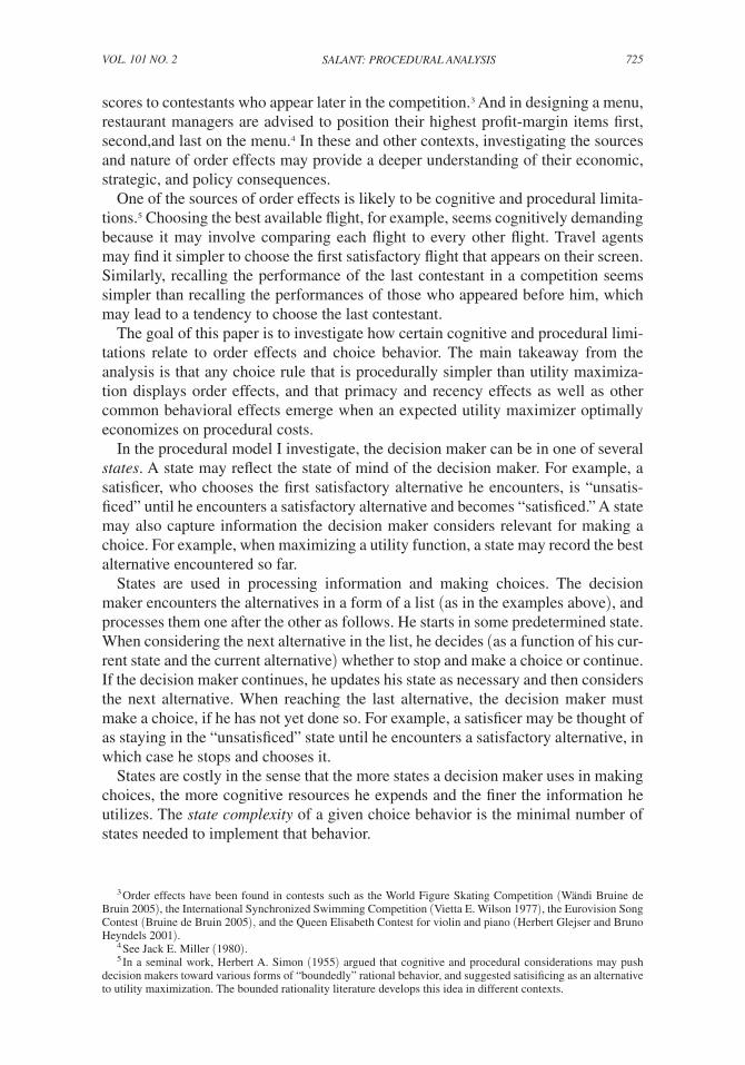
Satisficing. Consider a decision maker who classifies the alternatives 3 and 4 as satisfactory and the alternatives 1 and 2 as nonsatisfactory. He chooses from every list the first satisfactory element, or the last element if the list contains no satisfac-tory elements.

The one-state automaton in Figure 1 implements this satisficing procedure. The circle in the figure is the initial state q0 of the automaton. The Stop sign represents the ability of the automaton to stop. Edges represent transitions: the automaton stays in state q0 as long as it sees nonsatisfactory elements (i.e., 1 or 2); once it sees a sat-isfactory element (i.e., 3 or 4) it stops. The mapping x→x below state q0 describes the output of the automaton in state q0 : if the automaton is in state q0 and x is the last element in the list or g( q0 , x)=Stop, then the automaton outputs x.

Given a list, the automaton in Figure 1 reads the elements of the list in order. It stays in state q0 until it encounters a satisfactory element, in which case it stops and outputs that element. If it did not stop before reaching the end of the list, then the list contains no satisfactory elements and the automaton outputs the last element in the list. Thus the automaton in Figure 1 implements the satisficing procedure above.

13 In the computer science literature, an automaton in which the output function depends on both the state and the current input is called a Mealy machine. See George H. Mealy (1955).


Note that without enabling an automaton to condition its output on the element it currently processes, implementing satisficing would require four states because every alternative among 1, 2, 3, and 4 is a possible output.

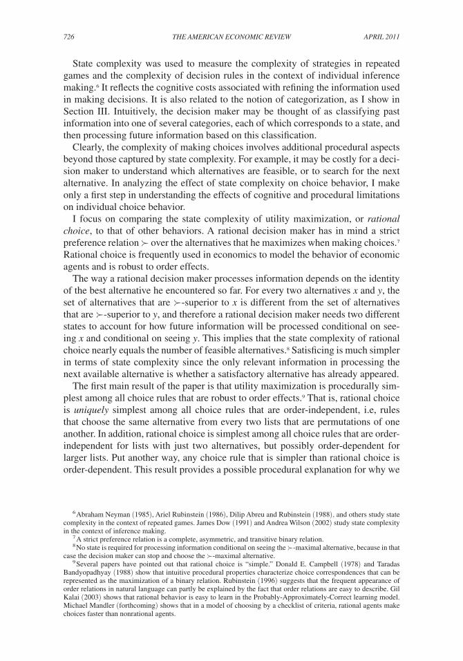
Maximizing with a Bias. Consider a decision maker who maximizes with a bias. He assigns the value u(1)=0 to the alternative 1, the value u(x)=x to x=2, 3, 4, and a bonus of b=1.5 to his favorite alternative. The decision maker designates the first alternative in the list as a favorite. When encountering the element x, he desig-nates x as the new favorite if u(x)>u(y)+b, where y is the current favorite. When the list ends, the decision maker chooses the current favorite.

The three-state automaton in Figure 2 implements a maximizing with a bias pro-cedure based on these primitives. The left-most state in the figure q0 is the initial state that describes how the automaton processes information in the beginning of the list. States q1 and q2 describe how the automaton processes information after seeing the element 2 and after seeing the element 3. For example, the automaton ignores the element 3 in state q1 (i.e., g( q1 , 3)=q1 and f ( q1 , 3)=2) because in state q1 the decision maker designates the element 2 as a favorite and hence considers 2 superior to 3.

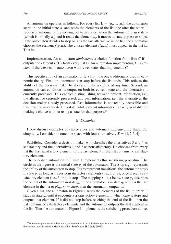
Note that the automaton in Figure 2 is not efficient. When the decision maker encounters the alternative 3 in state q0 , he considers it superior to every other alter-native. He can therefore stop and choose it. Hence, by omitting state q2 and defining g( q0 , 3)=Stop, we obtain an automaton with fewer states that implements the same procedure. This construction is illustrated in Figure 3.

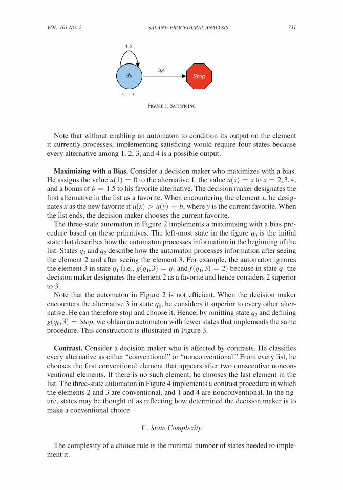
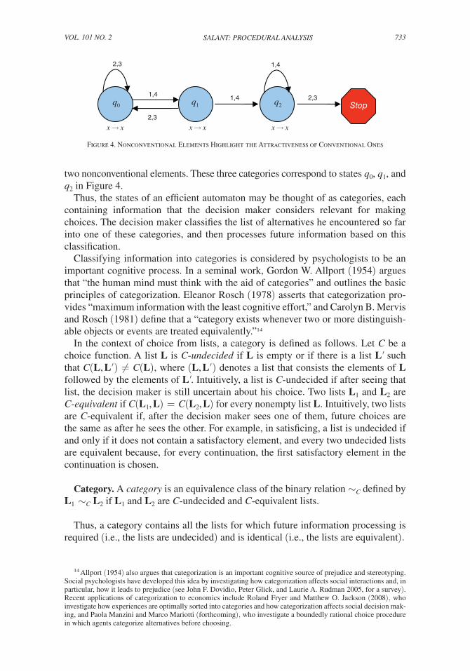
Contrast. Consider a decision maker who is affected by contrasts. He classifies every alternative as either “conventional” or “nonconventional.” From every list, he chooses the first conventional element that appears after two consecutive noncon-ventional elements. If there is no such element, he chooses the last element in the list. The three-state automaton in Figure 4 implements a contrast procedure in which the elements 2 and 3 are conventional, and 1 and 4 are nonconventional. In the fig-ure, states may be thought of as reflecting how determined the decision maker is to make a conventional choice.

C. State complexity

The complexity of a choice rule is the minimal number of states needed to imple-ment it.

Figure 1. Satisficing

1,2

3,4q0 Stop

x → x


State Complexity. The state complexity of a choice function from lists is the num-ber of states in an efficient automaton implementing the choice function.

State complexity reflects the number of different ways in which a decision maker processes information. Consider, for example, the maximizing with a bias proce-dure. In this procedure, the decision maker processes information in two differ-ent ways, depending on whether the element 2 appears before the element 3 or not. If 2 appears before 3, the decision maker ignores 3 because u(3)<u(2)+b. Otherwise, the decision maker chooses 3 because u(3)+b is higher than the utility of any other element. Hence, the decision maker can classify the list of alternatives encountered so far into one of two categories depending on whether the list includes the element 2 or not, and then process future information based on this classifica-tion. These two categories correspond to states q1 and q0 in Figure 3.

The contrast example also illustrates the connection between states and classify-ing information into categories. In this example, a decision maker who has not yet decided can classify the list of alternatives he encountered so far into one of three categories depending on whether (i) it ends with a conventional element; (ii) it ends with a nonconventional element preceded by a conventional one; and (iii) it ends with

Figure 2. Maximizing with a Bias (1)

q0

4

4

12

3

1,2,3

q1

Stop

q2

Stop1,2,3,4

x → x

x → 3

1,2,3 → 24 → 4

Figure 3. Maximizing with a Bias (2)

Stop

2 4

1

Stop

3,4

q0

x → x

q1

1,2,3

1,2,3 → 2,4 → 4


two nonconventional elements. These three categories correspond to states q0 , q1 , and q2 in Figure 4.

Thus, the states of an efficient automaton may be thought of as categories, each containing information that the decision maker considers relevant for making choices. The decision maker classifies the list of alternatives he encountered so far into one of these categories, and then processes future information based on this classification.

Classifying information into categories is considered by psychologists to be an important cognitive process. In a seminal work, Gordon W. Allport (1954) argues that “the human mind must think with the aid of categories” and outlines the basic principles of categorization. Eleanor Rosch (1978) asserts that categorization pro-vides “maximum information with the least cognitive effort,” and Carolyn B. Mervis and Rosch (1981) define that a “category exists whenever two or more distinguish-able objects or events are treated equivalently.”14

In the context of choice from lists, a category is defined as follows. Let c be a choice function. A list L is c-undecided if L is empty or if there is a list L′ such that c(L, L′)≠c(L), where (L, L′) denotes a list that consists the elements of L followed by the elements of L′. Intuitively, a list is c-undecided if after seeing that list, the decision maker is still uncertain about his choice. Two lists L1 and L2 are c-equivalent if c( L1, L)=c( L2, L) for every nonempty list L. Intuitively, two lists are c-equivalent if, after the decision maker sees one of them, future choices are the same as after he sees the other. For example, in satisficing, a list is undecided if and only if it does not contain a satisfactory element, and every two undecided lists are equivalent because, for every continuation, the first satisfactory element in the continuation is chosen.

Category. A category is an equivalence class of the binary relation ∼c defined by L1 ∼c L2 if L1 and L2 are c-undecided and c-equivalent lists.

Thus, a category contains all the lists for which future information processing is required (i.e., the lists are undecided) and is identical (i.e., the lists are equivalent).

14 Allport (1954) also argues that categorization is an important cognitive source of prejudice and stereotyping. Social psychologists have developed this idea by investigating how categorization affects social interactions and, in particular, how it leads to prejudice (see John F. Dovidio, Peter Glick, and Laurie A. Rudman 2005, for a survey). Recent applications of categorization to economics include Roland Fryer and Matthew O. Jackson (2008), who investigate how experiences are optimally sorted into categories and how categorization affects social decision mak-ing, and Paola Manzini and Marco Mariotti (forthcoming), who investigate a boundedly rational choice procedure in which agents categorize alternatives before choosing.

Figure 4. Nonconventional Elements Highlight the Attractiveness of Conventional Ones

1,42,3

1,4 1,4 2,3q0

2,3

Stopq1 q2

x → x x → x x → x


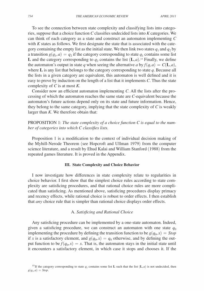
To see the connection between state complexity and classifying lists into catego-ries, suppose that a choice function c classifies undecided lists into K categories. We can think of each category as a state and construct an automaton implementing c with K states as follows. We first designate the state that is associated with the cate-gory containing the empty list as the initial state. We then link two states q1 and q2 by a transition g( q1 , a)=q2 if the category corresponding to state q1 contains some list L and the category corresponding to q2 contains the list (L, a).15 Finally, we define the automaton’s output in state q when seeing the alternative a by f(q, a)=c(L, a), where L is any list that belongs to the category corresponding to state q. Because all the lists in a given category are equivalent, this automaton is well defined and it is easy to prove by induction on the length of a list that it implements c. Thus the state complexity of c is at most K.

Consider now an efficient automaton implementing c. All the lists after the pro-cessing of which the automaton reaches the same state are c-equivalent because the automaton’s future actions depend only on its state and future information. Hence, they belong to the same category, implying that the state complexity of c is weakly larger than K. We therefore obtain that:

PROPOSITION 1: the state complexity of a choice function c is equal to the num-ber of categories into which c classifies lists.

Proposition 1 is a modification to the context of individual decision making of the Myhill-Nerode Theorem (see Hopcroft and Ullman 1979) from the computer science literature, and a result by Ehud Kalai and William Stanford (1988) from the repeated games literature. It is proved in the Appendix.

III. State Complexity and Choice Behavior

I now investigate how differences in state complexity relate to regularities in choice behavior. I first show that the simplest choice rules according to state com-plexity are satisficing procedures, and that rational choice rules are more compli-cated than satisficing. As mentioned above, satisficing procedures display primacy and recency effects, while rational choice is robust to order effects. I then establish that any choice rule that is simpler than rational choice displays order effects.

A. Satisficing and Rational choice

Any satisficing procedure can be implemented by a one-state automaton. Indeed, given a satisficing procedure, we can construct an automaton with one state q0 implementing the procedure by defining the transition function to be g( q0 , x)=Stop if x is a satisfactory element, and g( q0 , x)=q0 otherwise, and by defining the out-put function to be f( q0 , x)=x. That is, the automaton stays in the initial state until it encounters a satisfactory element, in which case it stops and chooses it. If the

15 If the category corresponding to state q1 contains some list L such that the list (L, a) is not undecided, then g( q1 , a)=Stop.


automaton did not stop before reaching the end of the list, it outputs the last element in the list. Figure 1 illustrates this construction.

The other direction is also true: if a choice function can be implemented by a one-state automaton, then it can be represented as a satisficing procedure. To see this, consider an automaton with one state q0 that implements a choice function c. Because the automaton has only one state, it cannot use any past information (except for the fact that it has not stopped yet) in making choices. In particular, its output in state q0 , when seeing an element x, must be x (otherwise, the automaton outputs an incorrect choice from some one-element list). Labeling an element x as satisfactory if the automaton stops when seeing it, and as nonsatisfactory otherwise, we obtain that c is consistent with choosing the first satisfactory element from every list, or the last element in the list if no satisfactory element appears in the list. Thus:

PROPOSITION 2: A choice function has minimal state complexity if and only if it can be represented as a satisficing procedure.

Rational choice is more complicated than satisficing. Intuitively, in rational choice, information processing depends on the identity of the best element seen so far, and hence the complexity of rational choice nearly equals the number of feasible alternatives.

PROPOSITION 3: the procedural complexity of rational choice is n−1, where n=|| is the number of feasible alternatives.

To see that fewer than n−1 states do not suffice for implementing rational choice, let xmax and xmin denote the utility maximal element and the utility minimal element in the outcome space . Suppose the decision maker encounters an alterna-tive x ≠xmax in the beginning of a list. Because xmax may appear down the list, the decision maker cannot stop when seeing x, and because x is a possible choice, the decision maker cannot move to the same state he would have moved to were y ≠x the first element in the list (since in this case the decision maker will not know which element of x and y to choose if xmin would be the second and last element). Thus, the decision maker needs at least a number of states that is equal to the number of elements in the outcome space excluding xmax, i.e., n−1 states.

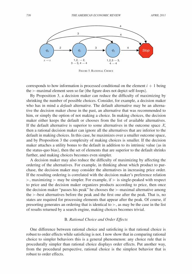
To see that n−1 states suffice for implementing rational choice, note that when seeing xmax, the decision maker can stop and choose it. When seeing any other element x in the beginning of the list, the decision maker can move to a state that “records” that x was seen.16 In this state, the decision maker ignores alternatives that are inferior to x, and when encountering an alternative y that is superior to x, the decision maker moves to a state that records y. The decision maker continues processing information in this fashion until xmax appears, in which case he stops and chooses xmax, or the list ends, in which case he chooses the utility-higher alternative among the one recorded in the current state and the last alternative. Figure 5 illustrates this construction for the case of maximizing the preference relation 4 ≻3 ≻2 ≻1. In the figure, state qi

16 Think about the initial state as recording that xmin was seen.


corresponds to how information is processed conditional on the element i+1 being the ≻-maximal element seen so far (the figure does not depict self-loops).

By Proposition 3, a decision maker can reduce the difficulty of maximizing by shrinking the number of possible choices. Consider, for example, a decision maker who has in mind a default alternative. The default alternative may be an alterna-tive the decision maker chose in the past, an alternative that was recommended to him, or simply the option of not making a choice. In making choices, the decision maker either keeps the default or chooses from the list of available alternatives. If the default alternative is superior to some alternatives in the outcome space , then a rational decision maker can ignore all the alternatives that are inferior to the default in making choices. In this case, he maximizes over a smaller outcome space, and by Proposition 3 the complexity of making choices is smaller. If the decision maker attaches a utility bonus to the default in addition to its intrinsic value (as in the status-quo bias), then the set of elements that are superior to the default shrinks further, and making choices becomes even simpler.

A decision maker may also reduce the difficulty of maximizing by affecting the ordering of the alternatives. For example, in thinking about which product to pur-chase, the decision maker may consider the alternatives in increasing price order. If the resulting ordering is correlated with the decision maker’s preference relation ≻, maximizing ≻ may be simpler. For example, if ≻ is single-peaked with respect to price and the decision maker organizes products according to price, then once the decision maker “passes his peak” he chooses the ≻-maximal alternative among the ≻-best alternatives before the peak and the first one after the peak. That is, no states are required for processing elements that appear after the peak. Of course, if presorting generates an ordering that is identical to ≻, as may be the case in the list of results returned by a search engine, making choices becomes trivial.

B. Rational choice and order Effects

One difference between rational choice and satisficing is that rational choice is robust to order effects while satisficing is not. I now show that in comparing rational choice to simpler behaviors this is a general phenomenon: any choice rule that is procedurally simpler than rational choice displays order effects. Put another way, from the procedural perspective, rational choice is the simplest behavior that is robust to order effects.

Figure 5. Rational Choice

3

4

4

4

32

q0 q1 q2 Stop

x → x 1,2, → 2,3 → 3, 4 → 4

1,2,3 → 3,4 → 4


Order-independent choice. A choice function c is order-independent if for every list (a1 , a2 , … , ak ) and every permutation σ of {1, … k}, it holds that c(a1 , a2 , … , ak )=c(aσ(1), aσ(2), … , aσ(k)). Thus, a choice function is order-independent if changing the ordering of the alternatives does not affect choice behavior. If a choice function c satisfies this condition only for k=2, then c is order-independent for pairs.

Order-independent choice functions can be classified according to whether they are rationalizable or not. A choice function c is rationalizable if there exists a pref-erence relation ≻ such that for every list L, c(L) is the ≻-maximal element in L. Otherwise, c is not rationalizable.

THEOREM 1: If a choice function is order-independent for pairs then it is at least as complicated as rational choice. If a choice function is order-independent and is not rationalizable, then it is strictly more complicated than rational choice.

Theorem 1 implies that any choice function that is simpler in terms of state com-plexity than rational choice inevitably displays order effects. If the state complexity of a choice function is smaller than that of rational choice, then there are two alternatives, a and b, such that the decision maker either chooses the first alternative from both lists, (a, b) and (b, a), or the second alternative from both lists. If the state complexity of a choice function c is equal to that of rational choice and c is not rationalizable, then changing the order of the alternatives in some list (not necessarily a list of two alternatives) alters choice behavior. This provides a possible procedural explanation for order effects: by using the order, the decision maker can simplify the complexity of making choices.

Theorem 1 also implies that every standard choice function that is not affected by order and cannot be described by the maximization of a preference relation is more complicated than maximizing a preference relation. Examples of such choice func-tions include Luce and Raiffa’s frog legs procedure, Sen’s tea party procedure, and Simonson and Tversky’s compromise procedure. In these, and in any other standard choice function that is not rationalizable, making choices depends on information beyond the alternative that the decision maker would choose if the list ended now. This implies a higher state complexity than in rational choice in which information processing depends only on the alternative that would be chosen if the list ended now.

Theorem 1 extends to certain forms of repetition effects. A choice function c is repetition-independent if c(L)=c(L, x)=c(x, L) for every list L and for every element x that appears in L. That is, a choice function is repetition-independent if adding an element that already appears in the list to the beginning or to the end of the list does not alter choice. If this condition holds only for two-element lists, then c is repetition-independent for pairs.

Repetition-independence implies order-independence. Indeed, if c is repetition-independent for pairs, then c(a, b)=c(a, b, a)=c(b, a) for every two elements a and b, and thus c is order-independent for pairs. Similarly, if c is repetition-independent, then it is order-independent.17 Thus:

17 Otherwise, if c is order-dependent, then there exist lists L1 and L2 that are permutations of one another such that c( L1)≠ c(L2 ). By repetition independence, however, we obtain that c( L1)=c( L1, L2)=c( L2).


COROLLARY 1: If a choice function is repetition-independent for pairs, then it is at least as complicated as rational choice. If a choice function is repetition-inde-pendent and is not rationalizable, then it is strictly more complicated than rational choice.

I now prove Theorem 1, relegating the technical details to the Appendix.

PROOF OF THEOREM 1. To prove the first part of the theorem, consider an automaton implementing a

choice function c that is order-independent for pairs. If the automaton stops after seeing an element x in the beginning of a list, then it cannot stop after seeing a dif-ferent element y in the beginning of a list. Otherwise, the automaton chooses the first element from the lists (x, y) and (y, x), violating order-independence for pairs. Similarly, the automaton cannot move to the same state q after seeing an element a in the beginning of a list and after seeing an element b ≠a in the beginning of the list. Otherwise, if c(a, b)=a, then the automaton moves to state q after seeing a, and then outputs f(q, b)=a. But this implies that the automaton also chooses a from the list (b, b) and thus does not implement c.

To summarize, in order to keep track of the information required to implement c, an automaton needs to process every element (excluding at most one element) using a different state. The automaton therefore has a number of states that is equal to or larger than the number of elements in the outcome space (excluding at most one ele-ment), implying that c is at least as complicated as rational choice.

To prove the second part of the theorem, let c be an order-independent choice function. By the first part of the theorem, the state complexity of c is at least n−1. Thus, to conclude the proof, it is enough to show that if the state complexity of c is exactly n−1, then c is rationalizable.

The following two Lemmas that are proved in the Appendix assert (i) that c has a “best” element that is chosen whenever it is available and a “worst” element that is never chosen whenever other elements are available, and (ii) that c is robust to repetition effects.

LEMMA 1: If a choice function c is order-independent and has complexity n−1, then there are two elements xmax and xmin such that c(xmax, L)=xmax for every list L and c(xmin, L)=c(L) for every list L that contains elements other than xmin.

LEMMA 2: If c is order-independent and has complexity n−1, then c(a, L)=c(L) for every list L and for every element a that appears in L.

Consider an automaton with n−1 states implementing c. By Lemma 1, when seeing an element x ≠xmax in the beginning of a list, the automaton cannot stop because the element xmax may appear down the list. In addition, the automaton can-not move to the same state after seeing x in the beginning of a list and after seeing a different element y in the beginning of a list because the next and last element may be the worst element xmin, in which case the automaton will not know whether to output x or y. We can thus identify any state q with a unique element x∈\{ xmax } that triggers the transition to state q when it appears in the beginning of the list.


By Lemma 2, c is defined over sets, i.e., neither order nor repetition affects choice behavior. Therefore, to prove that c is rationalizable, it is enough to show that c sat-isfies the Independence of Irrelevant Alternatives (IIA) property. The IIA property says that omitting an alternative that is not chosen from a choice problem does not alter choice. In the context of choice from sets, it is well known that a choice func-tion satisfies the IIA property if and only if the function is rationalizable.

Assume, to the contrary, that c violates the IIA property. Then, there exists a set of alternatives and an element x ∉ such that c( L, x)∈ but c( L, x) ≠c(L),where L denotes some listing of the elements of the set . That is, although x is not chosen from ( L, x), choice behavior is affected by omitting x from ( L, x).

The list L does not include the element xmax; otherwise by Lemma 1, the element xmax would be chosen from both L and (L, x). Hence, as the automaton processes the elements of the list L, it does not stop because xmax may appear down the list. Moreover, after processing the elements of L, the automaton reaches the state q associated with the element c(L) (were it moved to any other state and xmin was the next and last element, the automaton would output an incorrect choice).

Thus, because of the lack of states, the automaton reaches the same state after processing the element c( L) and the list L. Therefore, the automaton outputs the same alternative y from the lists (c( L), x) and ( L, x). This means that the automa-ton fails to implement c. Indeed, if y ≠c(L, x), then the automaton outputs an incorrect choice from ( L, x), and if y=c( L, x), then the automaton outputs an infeasible choice from (c( L), x) because we picked the set and the element x so that (i) the element c( L) differs from y (because y=c( L, x) and c( L)≠c(L, x)), and (ii) the element x differs from y (because y=c( L, x)∈ and x ∉). We therefore obtain that c satisfies IIA and hence it is rationalizable.

IV. Choice Design

Rational choice requires using different states to process different alternatives. This may be cognitively demanding, especially when the number of feasible alter-natives is large. For example, when choosing among flights, the number of possible choices may be very large and processing every flight differently may be compli-cated. In such cases, the decision maker may replace utility maximization with a choice procedure that is “close” to maximizing utility but uses fewer states.

Theorem 1 establishes that any choice rule that uses fewer states than rational choice displays order effects. Theorem 1 is silent, however, on the nature of these order effects. In this section, I explore what order and other framing effects emerge when a decision maker optimally approximates rational choice using a simpler choice rule.

The first step in investigating this question is to specify how well a given choice rule performs with respect to utility maximization. This depends on which lists the decision maker is expected to choose from, which depends in turn on the process that generates lists. In some cases, the choice designer may not have a clear per-ception of this process. He may then be interested in a choice rule that performs well in the worst possible case. In other cases, the designer may know the details of the process that generates lists. He may then use a measure of performance that depends on the specific process, such as maximizing expected utility. Both


maximizing expected utility and performing well in the worst case result in choice rules that display similar framing effects. I will focus on maximizing expected utility, and comment on performing well in the worst case when stating the main result of this section.

In what follows, lists are assumed to be generated by a stationary process. The first element in the list is drawn according to a probability measure P over the out-come space , where P(x)>0 for every x∈. With probability μ>0, the pro-cess ends. With probability 1−μ, the process continues and an additional element is drawn according to P. The process continues in this fashion until the list ends.

Given a choice function c and a utility function u, let u(c(L)) denote the utility of the element c chooses from the list L, and let E(u(c(L))) denote the expected utility c obtains, where the expectation is taken with respect to the process above. The objective of the following choice design problem is to maximize expected util-ity subject to having only K states to process information:

maxc:comp(c)=K

E(u(c(L))),

where comp(c) denotes the state complexity of c.18

When there is only one state, the decision maker cannot use any past informa-tion in making choices. Hence, when encountering an alternative he either stops and chooses it or ignores it, depending on whether the utility of that alternative is higher than the value of continuing. If the utility of the current alternative exceeds the continuation value, then the alternative is satisfactory and the decision maker stops and chooses it. Otherwise, the alternative is not satisfactory and the decision maker continues to the next alternative. Thus, the decision maker satisfices with an aspiration level that corresponds to the continuation value.

When K>1 states are available, the decision maker can use K−1 pieces of information in making choices (in the initial state, he cannot use any past informa-tion). In the optimal solution, these pieces of information correspond to K−1 dif-ferent alternatives because the process that generates lists is stationary. The decision maker maximizes for these K−1 “pivotal” alternatives. Processing the remain-ing alternatives is done as follows. The decision maker sets an aspiration level in the initial state and K−1 additional aspiration levels that are associated with the K−1 pivotal alternatives. When seeing an alternative x that is not pivotal, the deci-sion maker satisfices with the current aspiration level: he chooses x if x exceeds the current aspiration level, and ignores x otherwise. The current aspiration level is the initial aspiration level as long as the decision maker did not encounter a pivotal ele-ment, and the aspiration level associated with the best encountered pivotal element afterward.

More formally, a K-phase satisficing procedure is characterized by an initial aspi-ration level t0 and K−1 higher aspiration levels t1 <…<tK−1 that correspond to K−1 pivotal alternatives a1 , … , aK−1 , such that u( a1 )<…<u( aK−1 ). For every list, the decision maker starts in phase 0 and satisfices with the aspiration threshold

18 It is straightforward to extend the analysis to situations in which each state is costly and the designer also chooses the number of states.


t0 until he encounters an element aj and moves to phase j>0. In phase j, the next element x in the list is processed as follows (see Figure 6 for an illustration):

(i) If x is the last element in the list, the decision maker chooses the u-maximal element among aj and x.

(ii) If x= ai and u(x)>u(aj ), the decision maker switches to phase i.

(iii) Otherwise, the decision maker satisfices with the threshold tj : if u(x)>tj he chooses x and stops, and if u(x)≤tj he ignores x and stays in phase j.

THEOREM 2: Any choice function with state complexity K that maximizes expected utility can be represented by a K-phase satisficing procedure.19

By Theorem 2, the optimal way of approximating rational choice with K states is to maximize over K−1 pivotal alternatives and to satisfice (conditional on the best encountered pivotal element) for the remaining alternatives. Operationally, this K-phase satisficing procedure is simpler than utility maximization in the sense that the decision maker rank-orders only a few alternatives. The remaining alternatives are not fully evaluated, but rather are compared only to the pivotal elements and the corresponding thresholds. Hence, this procedure uses a coarser classification of information than rational choice.

A K-phase satisficer displays several behavioral effects. First, he displays a pri-macy effect: by moving an element (except maybe the last) toward the beginning of the list, the likelihood that the decision maker will choose that element increases. This is so because aspiration levels increase along the list and because the decision

19 Theorem 2 extends to minimizing the worst-case performance as follows. Given a list L, let u(L) be the util-ity of the u-maximal element in L, and let u(c(L)) be the utility of the element that c chooses from L. The regret of c with respect to u, regre tu (c)=maxL∈ℒ {u(L)−u(c(L))}, is the maximal utility loss associated with making choices according to c rather than maximizing u, where ℒ is the set of all nonempty lists. When the choice designer seeks to minimize the regret associated with making choices, i.e., solve minc:comp(c)=K regre tu (c), it can be shown that subject to two efficiency refinements, the generically unique choice function that solves this problem is a K-phase satisficing procedure.

Figure 6. History-Dependent Satisficing

Phase j

Stop

Phase iu(x) ≤ tj

u(x) > tj

x = ai

u(x) > u(aj)


maker chooses the first element above the current aspiration level. Second, the deci-sion maker displays a mild recency effect: by moving an element x that is not chosen to the last position in the list, it may be chosen. This could happen when the utility of x is smaller than the current aspiration level but larger than the utility of the cor-responding aspiration element. In such a case, the decision maker ignores x in the middle of the list because the continuation value is high, but chooses x if it appears last.

Moreover, for a K-phase satisficer, having more choices is not necessarily better: adding an element x to a list L may result in a utility-inferior choice, either because x is satisfactory but the utility of x is smaller than that of the element previously chosen from L, or because x is a pivotal element that increases the aspiration level enough so that a previously chosen alternative is no longer chosen. This may be interpreted as an example of the choice overload hypothesis (see Iyengar and Lepper 2000).

Finally, when the decision maker is endowed with a default alternative, he may display a tendency to favor the default over alternatives with higher utility. Indeed, in the presence of a default alternative, the decision maker’s aspiration level in the initial phase will be higher than the utility of the default because the decision maker has the option of choosing the default. Thus, the decision maker will ignore ele-ments with utility higher than that of the default but lower than the initial aspiration level, except maybe the last alternative in the list.

V. Concluding Remarks

This paper investigated one procedural aspect of making choices. I considered automata implementing choice rules, and measured the procedural complexity of a given choice rule by the minimal number of states required for implementing it. State complexity reflects the amount of information processing involved in making choices.

In rational choice, information processing depends on the identity of the best alternative considered so far, so the complexity of rational choice nearly equals the number of feasible alternatives. When the number of feasible alternatives is large, rational choice may therefore be cognitively demanding. In this case, a decision maker may replace maximization with a simpler choice rule to economize on pro-cedural costs.

The paper establishes that in order to simplify the complexity of making choices, the decision maker has to take advantage of the order in which the alternatives appear. Doing so optimally results in more concrete order effects, including primacy and recency effects, and in additional behavioral regularities, including choice over-load and default tendency. These effects emerge as optimal when a rational decision maker economizes on procedural costs.

In evaluating these results, one should keep in mind that there are cognitive and procedural aspects that are not captured by state complexity. In a basic search model, for example, the source of procedural complexity is the “marginal” cost associated with searching for the next element in a list rather than the “fixed” cost of imple-menting the choice rule. Analyzing how state complexity interacts with this and other procedural aspects is clearly important for gaining a deeper understanding of various behavioral regularities. This is a task for future research.


APPENDIX

A. Proof of Proposition 1

Fix a choice function c such that ∼c has K equivalence classes. It is enough to show that the state complexity of c is K. To do so, I first show that any automaton implementing c has≥K states. I then construct an automaton with K state imple-menting c.

To see that any automaton implementing c has≥K states, assume to the contrary that there exists an automaton with fewer than K states that implements c. Because the number of ∼c -equivalence classes is K, there are K undecided lists, L1, … , LK,such that every two of them are not equivalent. Because these lists are undecided, does not stop while or after processing any of them. Because has fewer than K states, there are two lists, Li and Lj, such that reaches the same state after process-ing any of them. But then chooses the same element from ( Li, L) and ( Lj, L) for every continuation L, in contradiction to Li and Lj not being equivalent.

I now construct an automaton with K states that implements c. Denote the equivalence class of an undecided list L by [L]∼c . The states of are the K equiva-lence classes of ∼c . The initial state is the equivalence class of the empty list. The transition function maps a state q and an element a∈ to another state as follows: take any list L in the equivalence class q and move to state [(L, a) ]∼c if the concat-enated list (L, a) is undecided; if (L, a) is decided (i.e., (L, a) is not undecided), Stop. Let f(q, a)=c(L, a) for some list L in q.

The functions f and g are well-defined functions. Indeed, assume L1∼c L2. Then c( L1, a)=c( L2, a) for every element a and thus f is well defined. In addition, because L1 and L2 are undecided and c( L1, L)=c( L2, L) for every nonempty list L, the list ( L1, a) is undecided if and only if ( L2, a) is undecided. If both are unde-cided, then ( L1, a) ∼c ( L2, a). Thus g is well defined.

It remains to show that implements c. I do so by induction on the length of the list. For every one-element list L=(a), the automaton outputs f( q0 ,(a))=c(L, a) for every list L in the equivalence class q0 . By taking L to be the empty list, we obtain that outputs c(a) as required. Consider a list L=(L′, a) where L′ is non-empty. If L′ is undecided, then by construction reaches state [L ′]∼c after reading L′. Since a is the last element in the list, outputs f([L ′]∼c , a). By the definition of f, f([L′]∼c , a)=c(L′, a)=c(L). If L′ is decided, denote by L″ the shortest begin-ning of L′ that is decided. By construction, the element chooses from L is the element chooses from L″. By the induction assumption, the element chooses from L″ is c(L″), and by the fact that L″ is decided c(L″)=c(L). Thus, out-puts c(L) as required.

B. Proof of Lemmas Stated in the Proof of theorem 1

PROOF OF LEMMA 1: Consider an automaton with n−1 states implementing c. If there is no element

xmax such that c( xmax, L)=xmax for every list L, then the automaton never stops in the initial state, i.e., g( q0 , x)≠Stop for every x∈. Since the automaton has n−1 states and the number of feasible alternatives is n, there exist two elements


x and y such that the automaton moves to the same state q after seeing any of them in the beginning of the list, i.e., g( q0 , x)=g( q0 , y)=q. Assume without loss of generality that c(x, y)=c(y, x)=x. Then, when seeing y in state q, the automaton needs to output x because it is possible that the element that caused the transition to state q is x and thus the automaton needs to choose c(x, y). But this implies that the automaton outputs the element x from the list (y, y) and hence it does not implement c. Thus, there exists an element xmax as required. The proof of the second part of the Lemma is similar.

PROOF OF LEMMA 2: Consider an automaton with n−1 states implementing c. By Lemma 1 and the

explanation that follows Lemma 1 in the main text, we can identify any state q of the automaton with a unique element x∈\{ xmax } that triggers the transition to state q when x appears in the beginning of the list.

Let L be some list and a an element that appears in L. If a∈{ xmax, xmin}, then c(a, L)=c(L) by Lemma 1. Consider an element a ∉{ xmax, xmin}. Denote by L′ a sublist of L in which one instance of a is omitted. Because c is order-independent, c(L)=c(a, L′ ) and c(a, L)=c(a, a, L′). Thus, to prove that c(a, L)=c(L), it is enough to prove that c(a, L′)=c(a, a, L′ ), and to prove the latter equality, it is enough to prove that g( qa , a)=qa , where qa is the state to which the automaton moves after seeing a in the beginning of the list. Assume this is not the case. Then, g( qa , a)=qb , where qb is the state to which the automaton moves after seeing b in the beginning of the list (g( qa , a) ≠Stop because xmax may appear down the list). For the automaton to make a correct choice from the list (b, xmin), it must be that f( qb , xmin)=b, but then the automaton outputs b from the list (a, a, xmin), which is an incorrect choice. Thus, g( qa , a)=qa as required.

C. Proof of theorem 2

Because there is a finite number of choice functions with state complexity K, there exists a choice function c that solves maxc:comp(c)=K E(u(c(L))). Let be an automaton with K states implementing c, and denote its initial state by q0 and its remaining states (if K>1) by q1 , … , qK−1 . Let Vi =E(u(c(L))| qi ) be the continu-ation value associated with state qi . Denote by xmin the u-minimal element in the outcome space . The following Lemma characterizes the output function of .

LEMMA 3: In every state qi there exists an element ai ∈ such that f(qi , x)=argmax{u(ai ), u(x)} for every x∈. Moreover ai =xmin for i=0, and ai ≠xmin otherwise.

PROOF: Let i ={w |f(qi , x)=w for some x ≠w}. The set i contains at most one ele-

ment. To see this, assume to the contrary that i contains two different elements w1 and w2 such that u(w1 )>u(w2 ). Then always processes both alternatives w1 and w2 before reaching state qi . Redefine the output function in state qi to output w1 whenever it outputted w2 to obtain a new automaton that achieves a higher expected utility than . Thus i is either empty (e.g., in the initial state) or contains a single


element. Define ai =xmin if i is empty and otherwise define ai to be the unique alternative in i . We have that f(qi , x)=argmax{u(ai ), u(x)} for every x because otherwise we can redefine f(qi , x)=argmax{u(ai ), u(x)} to obtain an improvement over .

To complete the proof, assume to the contrary that ai =xmin for i ≠0. Then the output function in states q0 and qi is identical. In particular, there is no element w (expect maybe xmin) that the automaton always processes before reaching state qi . (If there were such an element, we could redefine the output function to obtain a new automaton that performs better than .)

This implies that Vi =V0 . To see this, note that if Vi >V0 , then we can obtain an improvement over by redefining the initial state to be qi . If V0 >Vi , then we can redefine the transition function in state qi to mimic the transition function in state q0 to obtain an improvement over .

But if V0 =Vi , then we can also construct a automaton ′ that performs better than by replacing state qi with a new state q′ as follows. First, we shift all the incoming transitions to state qi to enter state q0 instead (i.e., if g(q, x)=qi in then we define g(q, x)=q0 in ′ ). All other transitions and outputs in ′ are identical to . Because there are no incoming transitions to state qi in ′, we omit qi in ′. Thus ′ obtains the same expected utility as with one less state. We now add a state q′ to ′ that improves its performance as follows. Because ′ has K−1<n−2 states and there are n possible alternatives, there is an element w ∉{ xmin, xmax} such that either (i) g( q0 , w)=Stop; or (ii) g( q0 , w)=g( q0 , x)=qm for some element x. Suppose (i) holds. Define g( q0 , w)=q′, g(q′, x)=Stop and f(q′, x)=argmax{u(w), u(x)}. That is, q′ either outputs w or a u-higher element, and thus the expected utility conditional on seeing w in the initial state is now larger. Suppose (ii) holds. Then the output function in state qm is identical to the output function in q0 , and by the argument above, Vm =V0 . Define g( q0 , w)=q′, g(q′, x)=g( q0 , x) and f(q′, x)=argmax{u(w), u(x)} for every element x. By definition, the continuation value in state q′ is larger than Vm =V0 because q′ imitates q0 , except for sometimes output-ting an element with a larger utility. This implies that the expected utility conditional on seeing w in the initial state is now larger, and thus we obtain an improvement over .

Lemmas 4 and 5 characterize the continuation values in the different states.

LEMMA 4: If qi and qj are two states such that u(ai )>u(aj ), then Vi >Vj .

PROOF: Suppose not. Pick qj to be a state associated with u-smallest element aj for which

this happens (if there is more than one such state, pick qj to be the one with the high-est continuation value). Since the outputs in state qi are sometimes identical and sometimes u-larger than the outputs in state qj , the continuation value in state qj is weakly larger than in state qi only if there is a transition g( qj , x) ≠qj for some ele-ment x that results in a u-higher expected value than the transition g( qi , x) in state qi . But this is impossible because we can always replicate this transition in state qi and thus obtain a higher continuation value in state qi . Indeed, if g( qj , x)=Stop, then we can define g( qi , x)=Stop as well. Otherwise the transition g( qj , x) is to state qm such


that u( am )>u( aj ). (Because we picked aj so that all continuation values in states associated will u-lower elements are lower than Vj , we must have u( am )>u( aj ).) In this case, x=am . (It cannot be that am appears in all lists that reach state qj because then we would output am rather than aj in state qj .) We can thus replicate this transi-tion in state qi as well.

LEMMA 5: For every two states qi and qj , it holds that Vi ≠ Vj .

PROOF: Suppose Vi =Vj . Then ai =aj by Lemma 4, and the output function in states qi

and qj is identical. Suppose the automaton always processes an element y ≠ ai before reaching state qi . Then, u(y)<u(ai ) or else we would output y in state qi instead of ai . In addition, there is no sequence of transitions connecting state qi to a state qm such that f(qm , x)=argmax{u(y), u(x)} because this would imply a transition from some state with a higher continuation value to another state with a lower continua-tion value (following Lemma 4), contradicting the optimality of . Thus, the only relevant history in state qi is ai . Similarly, the only relevant history in state qj is aj = ai.Because the relevant history in both states is ai , we can use arguments similar to Lemma 3 and replace one of the states with a new state q′ such that the modified automaton achieves a higher expected utility.

By Lemma 5, we have that Vi ≠Vj for every 0<i ≠j ≤ K −1. This implies that ai ≠ aj because otherwise we would have Vi =Vj . Thus, by Lemmas 4 and 5, we can reorder the states such that V0 <V1 …<VK−1 and u(a0 )<u(a1 ) …<u(aK−1 ).For every i we also have that Vi >u(ai ) (or else we can define g(qi , x)=Stop and obtain an improvement over ).

To conclude the proof, I characterize the transition function of . Consider a transition g( qi , aj ) for j>i. Because Vj >Vi and Vj >u( aj )>u( ai ), we cannot have that g( qi , aj )∈{ qi , Stop}. Thus, g( q0 , aj )=qj . For i ≠0, we cannot have that (i) g( qi , aj )=q0 because Vj >V0 ; or that (ii) g( qi , aj )=qm for m>0, m ≠ i, j, because this implies that generates an infeasible choice from the list ( ai , aj , xmin). Thus, g( qi , aj )=qj for j>i. By similar arguments, if j≤i then g( qi , aj )=qi .

Consider a transition g( qi , x) for x ≠aj . We cannot have that g( qi , x)=qm with m>i because then outputs an infeasible choice from ( ai , x, xmin). We cannot have that g( qi , x)=qm with m<i because Vi >Vm . Thus, g( qi , x)∈{ qi , Stop}. By the optimality of , g( qi , x)=Stop if u(x)>Vi , and g( qi , x)=qi otherwise.

REFERENCES

Abreu, Dilip, and Ariel Rubinstein. 1988. “The Structure of Nash Equilibrium in Repeated Games with Finite Automata.” Econometrica, 56(6): 1259–81.

Allport, Gordon W. 1954. the nature of Prejudice. Reading, MA: Addison-Wesley.Bandyopadhyay, Taradas. 1988. “Revealed Preference Theory, Ordering and the Axiom of Sequential

Path Independence.” Review of Economic Studies, 55(2): 343–51.Bruine de Bruin, Wändi. 2005. “Save the Last Dance for Me: Unwanted Serial Position Effects in Jury

Evaluations.” Acta Psychologica, 118(3): 245–60.Campbell, Donald E. 1978. “Realization of Choice Functions.” Econometrica, 46(1): 171–80.


Copeland, Duncan G., Richard O. Mason, and James L. McKenney. 1995. “Sabre: The Develop-ment of Information-Based Competence and Execution of Information-Based Competition.” IEEE Annals of the History of computing, 17(3): 30–57.

Dovidio, John F., Peter Glick, and Laurie A. Rudman, ed. 2005. on the nature of Prejudice: Fifty years After Allport. Malden, MA: Blackwell Publishing.

Dow, James. 1991. “Search Decisions with Limited Memory.” Review of Economic Studies, 58(1): 1–14.Fryer, Roland, and Matthew O. Jackson. 2008. “A Categorical Model of Cognition and Biased Deci-

sion Making.” the B.E. Journal of theoretical Economics, 8(1). http://www.bepress.com/bejte/vol8/iss1/art6/.

Glejser, Herbert, and Bruno Heyndels. 2001. “Efficiency and Inefficiency in the Ranking in Compe-titions: The Case of the Queen Elisabeth Music Contest.” Journal of cultural Economics, 25(2): 109–29.

Ho, Daniel E., and Kosuke Imai. 2008. “Estimating Causal Effects of Ballot Order from a Random-ized Natural Experiment: The California Alphabet Lottery, 1978–2002.” Public opinion Quarterly, 72(2): 216–40.

Hopcroft, John E., and Jeffrey D. Ullman. 1979. Introduction to Automata theory: Languages and computation. Reading, MA: Addison-Wesley.

Iyengar, Sheena S., and Mark R. Lepper. 2000. “When Choice Is Demotivating: Can One Desire Too Much of a Good Thing?” Journal of Personality and Social Psychology, 79(6): 995–1006.

Kahneman, Daniel, Jack L. Knetsch, and Richard H. Thaler. 1991. “Anomalies: The Endowment Effect, Loss Aversion, and Status Quo Bias.” Journal of Economic Perspectives, 5(1): 193–206.

Kalai, Ehud, and William Stanford. 1988. “Finite Rationality and Interpersonal Complexity in Repeated Games.” Econometrica, 56(2): 397–410.

Kalai, Gil. 2003. “Learnability and Rationality of Choice.” Journal of Economic theory, 113(1): 104–17.King, Amy, and Andrew Leigh. 2009. “Are Ballot Order Effects Heterogeneous?” Social Science

Quarterly, 90(1): 71–87.Koppell, Jonathan GS, and Jennifer A. Steen. 2004. “The Effects of Ballot Position on Election Out-

comes.” Journal of Politics, 66(1): 267–81.Krosnick, Jon A., Joanne M. Miller, and Michael P. Tichy. 2004. “An Unrecognized Need for Ballot

Reform: The Effects of Candidate Name Order on Election Outcomes.” In Rethinking the Vote: the Politics and Prospects of American Election Reform, ed. Ann N. Crigler, Marion R. Just and Edward J. McCaffery, 51–73. New York: Oxford University Press.

Luce, R. Duncan, and Howard Raiffa. 1957. Games and decisions: Introduction and critical Survey. New York: Wiley.

Mandler, Michael. Forthcoming. “Rationality and the Speed of Decision-Making.” In Proceedings of the 12th conference on theoretical Aspects of Rationality and Knowledge.

Manzini, Paola, and Marco Mariotti. Forthcoming. “Categorize then Choose: Boundedly Rational Choice Welfare.” Journal of the European Economic Association.

Mealy, George H. 1955. “A Method for Synthesizing Sequential Circuits.” Bell Systems technical Journal, 34(5): 1045–79.

Meredith, Marc, and Yuval Salant. 2007. “The Causes and Consequences of Ballot Order-Effects.” SIEPR Discussion Paper 06-029.

Mervis, Carolyn B., and Eleanor Rosch. 1981. “Categorization of Natural Objects.” Annual Review of Psychology, 32: 89–115.

Miller, Jack E. 1980. Menu Pricing and Strategy. Boston, MA: CBI Publishing.Miller, Joanne M., and Jon A. Krosnick. 1998. “The Impact of Candidate Name Order on Election Out-

comes.” Public opinion Quarterly, 62(3): 291–330.Neyman, Abraham. 1985. “Bounded Complexity Justifies Cooperation in the Finitely Repeated Pris-

oner’s Dilemma.” Economics Letters, 19(3): 227–29.Rosch, Eleanor. 1978. “Principles of Categorization.” In cognition and categorization, ed. Eleanor

Rosch and Barbara B. Lloyd, 27–48 Hillsdale, NJ: Erlbaum.Rubinstein, Ariel. 1986. “Finite Automata Play Repeated Prisoner’s Dilemma.” Journal of Economic

theory, 39(1): 83–96.Rubinstein, Ariel. 1996. “Why Are Certain Properties of Binary Relations Relatively More Common

in Natural Language?” Econometrica, 64(2): 343–55.Rubinstein, Ariel, and Yuval Salant. 2006. “A Model of Choice from Lists.” theoretical Economics,

1(1): 3–17.Sen, Amartya. 1993. “Internal Consistency of Choice.” Econometrica, 61(3): 495–521.Simon, Herbert A. 1955. “A Behavioral Model of Rational Choice.” Quarterly Journal of Economics,

69(1): 99–118.


Simonson, Itamar, and Amos Tversky. 1992. “Choice in Context: Tradeoff Contrast and Extremeness Aversion.” Journal of Marketing Research, 29(3): 281–95.

US General Accounting Office. 1986. Airline competition: Impact of computerized Reservations Sys-tems. Resources, Community, and Economic Development Division. Washington, DC, May.

US Department of Justice. 1983. Advanced notice of Proposed Rulemaking – Airline computer Reser-vation Systems. EDR - 466, Docket No. 41686 (before the Civil Aeronautics Board).

Wilson, Andrea. 2002. “Bounded Memory and Biases in Information Processing.” nAJ Economics, 5. http://www.najecon.org/naj/cache/234936000000000070.pdf.

Wilson, Vietta E. 1977. “Objectivity and Effect of Order of Appearance in Judging of Synchronized Swimming Meets.” Perceptual and Motor Skills, 44(1): 295–98.

procedural analysis of choice rules with applications to ... · were listed on american’s...

Documents