Problems of Multiobjective Mathematical Programming and the Algorithms of their Solution

Volkovich, V.

IIASA Working Paper

WP-89-057

August 1989

Volkovich, V. (1989) Problems of Multiobjective Mathematical Programming and the Algorithms of their Solution. IIASA

Working Paper. IIASA, Laxenburg, Austria, WP-89-057 Copyright © 1989 by the author(s). http://pure.iiasa.ac.at/3287/

Working Papers on work of the International Institute for Applied Systems Analysis receive only limited review. Views or

opinions expressed herein do not necessarily represent those of the Institute, its National Member Organizations, or other

organizations supporting the work. All rights reserved. Permission to make digital or hard copies of all or part of this work

for personal or classroom use is granted without fee provided that copies are not made or distributed for profit or commercial

advantage. All copies must bear this notice and the full citation on the first page. For other purposes, to republish, to post on

servers or to redistribute to lists, permission must be sought by contacting repository@iiasa.ac.at

W O R K I N G P A P E R

Problems of Multiobjective Mathematical Programming and the Algorithms of their Solution

Victor Volkovich

August 1989 WP-89-57

I n t e r n a t i o n a l I n s t i t u t e for Applied Systems Analysis

Problems of Mult iobject ive Mathematical Programming and the Algorithms of their Solution

Victor Volkovich

August 1989 WP-89-57

Glushkov Institute of Cybernetics of the Ukr. SSR Academy of Sciences, Kiev U.S.S.R.

Working Papers are interim reports on work of the International Institute for Applied Systems Analysis and have received only limited review. Views or opinions expressed herein do not necessarily represent those of the Institute or of its National Member Organizations.

INTERNATIONAL INSTITUTE FOR APPLIED SYSTEMS ANALYSIS A-2361 Laxenburg, Austria

Foreword

Development of interactive Decision Support Systems requires new approaches and numerical algorithms for solving Multiple Objective Optimization Problems. These alg* rithms must be robust and efficient and applicable to possibly a broad class of problems. This paper presents the new algorithm developed by the author. The algorithm consists of two steps: (a) reduction of the initial Multiple Objective Optimization Problem into a system of inequalities, and (b) solving this set of inequalities by the iterative procedure proposed by the author. Due to its generality, the algorithm applies to various Multiple Criteria Optimization Problems, including integer optimization problems. The author presents several variants of the algorithm as well as results of numerical experiments.

Prof. A.B. Kurzhanski Chairman, Systems and Decision Sciences Program

Table of Contents

Page

1 . A General Approach to Solving Multiobjective Programming Problems ...................... 1

2 . The Algorithms Solving Multiobjective Mathematical Programming Problems ........... 6

3 . Method of Constraints Applied to Integer Problem Without Side Constraints ........... 12

4 . Computational Experience in Application of Method of Constraints to Lnteger Multi-Objective Problems [I] ......................................................................... 20

References ..................................................................................................................... 22

Problems of Mult iobjective Mat hemat ical Programming and the Algorithms of their Solution

Victor Volkovich

Glushkov Institute of Cybernetics of the Ukr. SSR

Academy of Sciences Kiev

U.S.S.R.

1. A General Approach to Solving Multiobjective Programming Problems

Let it be necessary to choose a certain decision z E DO by vector criterion

f = {fi(z)), i E I where Do is the region of admissible solutions from which the choice is

to be made.

I = {TM) is a set of indices of objective functions and Il = Il u I2 (Il is the index

of objective functions which are being maximized; I2 is the index of objective functions

which are being minimized).

It is well-known that the solution of multiobjective programming can not give o p

timum each objective function and must be a compromise solution. For definition a

compromise solution is necessary to execute heuristic procedures in originally staging of

problems. There are different ways for that; we will consider one of them [ I & 21. Let ex-

ecute the next two heuristic procedures. First, to introduce transformations of the objec-

tive functions, which permit of comparing them with each other, of the following form

It is first necessary, of course, first for each objective function optimal fP Vi E I2 and

worst fi mi,, Vi E Il and fi ,,, Vi E I2 values are calculated separately over the feasible

region Do. The transformation wi measures the degree to which the i-th objective func-

tion value departs from the ideal value towards the worst feasible value for this function.

We will call wi(fi(z)) the relative loss function for the i-th objective calculated over the

feasible region. The dimensional space defined by all the relative loss function wi(fi(z))

will be designated as W. Second of them to introduce the preference on a set criterion

functions in the numerical scale with the help of weighting coefficients

p E Q+ = {pi : pi > O,Vi E I, ziE pi = 1) particular, if the DM indicates this preference

for assigning desirable values to each objective function fi* E [f , fi max] if i E Il and

f E f i n , fi], if fi E 12, the preference can be calculated by the following expression

[I.] :

where w; defines value f; Vi E I in space W of transforming objective functions, and point

f * = {fit, Vi E I) define point w* = {w,* = wi(fi3, Vi E I ) in space W.

These heuristic procedures allow us to define a decision to the vector optimization

problem to mean that compromise decision which belongs to the no-inferior set and lies in

the direction defined by the section p E Q+ in space transforming objective function W.

Theorem 1. For solution zo E Do, such that wi(z0) > 0 for every i E I, to be a non-

inferior solution, it is sufficient for zo to be the only solution to the system of inequalities.

Piwi(zo) 2 ko for every i E I (3)

for the minimal value k* of parameter ko for which this system is consistent.

Proof: Suppose that the opposite is true, i.e., that the only solution zo of the system of

inequalities (1.14) where ko = k*, is not an efficient solution. Then there must exist an

alternative z1 E 0 such that wi(zl) 5 wi(zOf), for every i E I, with a t least one of these

inequalities holding strictly. Multiplying these inequalities by pi > 0, for every i E I, we

obtain piwi(~l) Piwi(~Of) k0f with a t least one of the left hand inequalities holding

strictly. This implies that z1 eatisfies (3) for ko = ki. But this contradicts the unique-

ness of solution zo. Therefore, zo must be a non-inferior solution.

This theorem forms the theoretical basis for the method of searching a compromise

decision of multiobjective programming problems. The method starts by transforming

the original problem into a system of inequalities consisting of (3) and the feasible region

expressed as inequalities in space W. Then parameter ko E (0,1/M) is successively re-

duced and the system of inequalities is checked for consistency. The process of reducing

ko and checking the inequalities for consistency continues until the inequalities are found

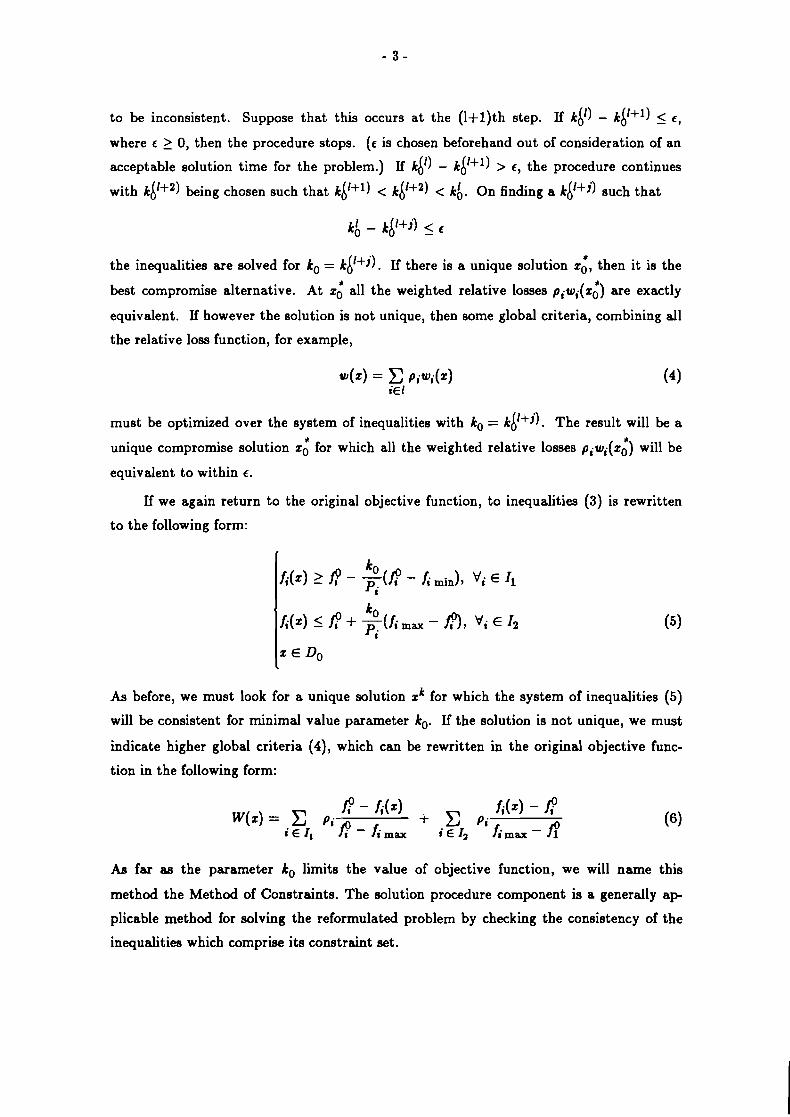
to be inconsistent. Suppose that this occurs at the (l+l)th step. If kA1) - k i l + l ) 5 e ,

where r 2 0, then the procedure stops. (r is chosen beforehand out of consideration of an

acceptable solution time for the ~roblem.) If kA1) - kA1+l) > r, the procedure continues

with kA'+2) being chosen such that ki1+1) < ti'+') < kb . On finding a kA1+j) such that

the inequalities are solved for ko = kA'+j). I f there is a unique solution z i , then it is the

best compromise alternative. At z i all the weighted relative losses piwi(zi) are exactly

equivalent. If however the solution is not unique, then some global criteria, combining all

the relative loss function, for example,

must be optimized over the system of inequalities with ko = kL1+j) . The result will be a

unique compromise solution 4 for which all the weighted relative losses Piwi(zi) will be

equivalent to within e.

If we again return to the original objective function, to inequalities (3) is rewritten

to the following form:

As before, we must look for a unique solution zk for which the system of inequalities (5)

will be consistent for minimal value parameter ko. If the solution is not unique, we must

indicate higher global criteria (4), which can be rewritten in the original objective func-

tion in the following form:

AB far as the parameter ko limits the value of objective function, we will name this

method the Method of Constraints. The solution procedure component is a generally a p

plicable method for solving the reformulated problem by checking the consistency of the

inequalitiea which comprise its constraint set.

There is a different way we can find indicating higher decision solving the problem of

the next form

where w;( f l ( z ) ) is defined in expression (1).

To acquire a clearer understanding of the algorithm, let's consider a 2-dimensional

illustrative example depicted in Figure 1.

We iteratively construct the feasible region by imposing increasingly tighter parti-

tions along the search ray. These partitions are obtained from the constraints defined by

p iw i ( z ) < kAr), i = 1,2, where ko is successively reduced until the remaining feasible re-

gion is sufficiently small to allow identification of a best compromise solution. Notice

that decreasing ko reduces all the weighted relative losses and thereby reduces the feasible

region into an increasingly smaller area. Thus, if we define n ( p ) as the constructed feasi-

ble region a t the p t h iteration, then as ko +'O all the relative loss functions approach

zero, i.e., the objective functions approach their optimal values. On the other hand, as

The best compromise solution C* is that feasible point for which the weighted rela-

tive losses are both equivalent and minimal, that is

Graphically, C* is that feasible point which is closest to the ideal point along the search

ray.

To find the best compromise solution, the Method of Constraints seeks the lowest

value of LA') for which the intersection of G and nIr) is not empty. G n f l # 0 as long as

the inequalities defining the problem's constraint set remain consistent. The method

derives its name from its iterative imposition of tighter constraints p iw i ( z ) < kAr) on the

original feasible region G.

In this approach we are not only concerned with a few objective functions and the

region of admissible solutions, but also notice that each step in this interactive procedure

must have effective algorithm checking the consistency of the system inequalities (5). We

consider the solving of different algorithms multiobjective programming problems based

on this approach.

Figure 1.

2. The Algorithms Solving Multiobjec tive Mathematical Programming Prob-

lems

We write a general form of problem with the set of linear objective function

linear constraints in general view

and constraints on each variables

There is a set J of index variables n, Q a set of index constraints, dimension

, c V E I, V E I, ai, , Vj E J , i E Q , bi, V, E Q is corresponding coefficients, dj(i) - the level boundary of change variable z,,d,(,) - the upper boundary of change variable z,

in the original statement problem.

If z, is continuous we usually have a linear programming problem with set objective

function and will denote it by MLP. If z, is non-continuous we have multiobjective linear

programming problem with integer variables and will denote it by MILP. In particular, if

d,(l) = 0, and dj(u) = 1 and variables are non-continuous, we will have multiobjective

linear programming problem with 0-1 integer variables (Bulev Variables) and will denote

it by MBLP.

Consider MLP problem. We will assume that the definition of the above heuristic

procedure was done. We know the value f = C c j z!('), Vi E I, and j € J

c<z(i) fi (mi.) = C cjzjikin) v i E 11 9 fi(max) = C J J (mu) j € J j€J

where

P ( ' ) = arg max(min) = C c j z j , r E DO Vi E 4 (Vi E 12) , j€J

and

= arg min C cj z j , r E Do , Vi E Il , j E I

( 1 = arg max = C c j z j , z E Do , Vi E I2 Zmax j E I

Do- region of admissible solutions denoted constraints (9) and (10). Using the Method of

Constraints reformulation of the MLP problem we get [3].

We must look for unique solution zk for which this system will be consistent to

minimal value parameter ko. We cannot consider interactive procedure with parameter

ko in this case and reformulated these problems to new problem linear programming.

min z,+~ = KO 2 I%+ 1

with constraints.

where

The problem (12) can be solved by using the simplex technique.

Consider MILP and MBLP problems. For these problems we will use interactive pro-

cedure of the Method of Constraints successively reducing the value of parameter ko and

then checking to see whether the inequalities comprising the constraint set a still con-

sistent. If so, the feasible set defined by these constraints is checked to see if it is small

enough to allow the solution to be found by an exhaustive search procedure. If so, the

search is performed and the method stops. If not, ko is once again reduced and procedure

is repeated until the feasible set is sufficiently small to permit the use of exhaustive search

procedure. If after uo has been reduced the inequalities in the constraint set are found to

be inconsistent, ko is increased and the constraints rechecked for consistency. For check-

ing constraint consistency we will use a procedure known as sequential analysis and sift-

ing decision, which Mikhalevich developed earlier for solving integer programming prob-

lems in general and the sequential analysis scheme proposed in [4-71 for the solution of the

discrete optimization problems. We will not go into details with all aspects of this a p

proach and refer readings to reset source [8] explaining some important matters. The gen-

eral view does not concern inequalities (11).

Denote n(O) = n [djf'd , d,(f ' i ) ] a parallelepiped within which the variables z,, j E J

vary at the original statement of problem. Consider arbitrary linear constraint

There is [ - I i j and [ - I i we will understand arbitrary coefficients right or left part of con-

straints (11).

Definition. The value A z,((j) or A z,(f'i) will name the level and upper correspondent

by tolerance of variables z, E id@) , d,(f'&] by constraint view (13) if from that value

zj c A z ~ ( ~ ) or Z, > A z,((L) follow that this value zj can not form admissible solution for

inequality (13).

Theorem 2. Value

ie the level tolerance of variable zj if [ - I i i > 0 and is the upper tolerance of variable zji if

[.Iij c 0, we I] denote the integer part from expression standing in brackets.

In the same way one can determine the set J? = { j : j E J , [.Iij > 0),

Proof. We will prove only one part of this theorem for accident when [ - I i j > 0. Let

value Ej for which

, - can form decision z' = zl' , .. ., 2j -1 , Z , , z,+~' , . .. , z,' satisfying inequality (14). Then

C [-Iipzp' + [ - I i j Zj 5 [ - I i . Rewrite this expression resetting manner P E J l j

where ~ ( ' 1 = [djph , dT(u)] we receive contradiction. J E J / ~

Basing this theorem on each step denoting value parameter ko for inequality (11) we

apply a procedure which builds the intervals of variation of each variables according elim-

ination principle which is applied for every constraints (11) on set Il U12 U Q .

If after applying this elimination principle the remaining set of values for any term

of decision z is empty, the Method of Sequential Analysis has revealed the constraint set

to be inconsistent and consequently the value assigned to ko was too small and so must be

increased and the procedure repeated.

On the other hand, if none of the remaining sets of vector component values turns

out to be empty, then the constraint set is still consistent. In this case, there are a

number of possibilities:

(1) If the set of remaining vector component values is still too large to allow the selec-

tion of the preferred decision by exhaustive analysis, then a lower value must be as-

signed to ko and the procedure repeated.

(2) If the number of remaining vector component values is not too great for exhaustive

analysis, then the decision(s) are found which minimize

(a) If a unique decision is found which satisfies the problem's constraints, then it is

the desired compromise solution.

(b) If there is not a unique decision then select the one that minimizes the global

criteria (4). If this decision z * satisfies the constraint set shown in (11) then i t is the

desired compromise solution. Decisions that meet the conditions stipulated in either (a)

or (b) are said to have met Criterion I for best compromise solutions.

(c) If the alternative found in (b) does not satisfy the constraints in (11) then the

initial problem's objective functions are required to satisfy the following additional new

constraints:

With these constraints added to the original problem (9) the Method of Sequential

Analysis is again employed to eliminate decision from the initial set V, producing either a

single decision or a set of decisions which will now satisfy the conditions described in (a)

or (b). Alternatives that meet the conditions stipulated in (c) are said to have met Cri-

terion I1 for best compromise solutions [I].

Consider a discrete separable programming problem with a set separable objective

function. Let X = Xi - a set of possible solutions where I XI = N = 11 Jj. In other J€ J j€ J

words, z is a vector consisting of n terms 2 = {q4) ., W4) I . - . I ). The j-th com-

ponent of vector z is denoted z,(lj) and takes on J, possible values, an arbitrary one of

which is the 1, -th. Let

a set of separable functions which we must find a compromise solution. The compromise

solution must belong to the possible solution system of constraints

The problem is then transformed into the Method of Constraints formulation. Substitut-

ing for view of objective functions (16) or constraints (17) the system inequalities (11) is

then rewritten.

where

0 In these sectors zi , zi(,,) , zi(min) it is found which optimize the objective functions for

z E X .

arg max fi(z) = C arg max fj(zj(lj)) 9; E Ii ZEX j~ J zi(lj)EXi

arg min fi(z) = C arg min fi(zj(lj)) ,i E I2 , zEX jEJ zi(lj)Exi

zi(maz) = arg max fi(z) = C arg m u fi(zj(,.)) , V i E I2 . +E 2 jE J zi(li)Ezi

We then define z/zj as any vector ii without its j-th component, i.e.

The condition used by the Method of Sequential Analysis t o eliminate vector com-

ponent values is

Eliminate vector component value z,(Q) from further consideration if the following is

true for any i = 1, ..., M.

where

In effect these conditions state: Assuming all components of vector z, except the j-

th component, are contributing the optimal possible value to objective function fi, then

eliminating any values for the j-th term of vector z that violate the constraint placed on

the i-th objective function by setting ko = t h h ) , namely the condition that

The above elimination principle is applied for every component z,, j = 1 , .-. n of

vector z and for every objective function fi(z)< i = 1 , -.- , M. In this elimination principle the remaining set of values for any term of vector z a p

plies by the scheme method of Sequential Analysis using the above analogy.

The results of computational experience and the application of the Method of Con-

straints to integer and separable multi-objective programming problems will become

clearer by considering the following.

3. Method of Constraints Applied to Integer Problem Without Side Con-

straints

An illustrative example of the application of the Method of Constraints to an integer

programming problem without side constraints. In the problem three objective functions

I11

are minimized over the set X = {XI x X2 x x X8)

Thus, z is a vector with eight terms all of which feasible values are represented

above in set z. From set z we see that there are 8640 possible combination values of vec-

tor z.

Each feasible vector component value zj(4) contributes $(z,(~~)) to the i-th objective

function, where i is the objective function index ( i = 1,2,3) and zj(1,) is the 1-th feasible

value for the j-th term of vector z. This can be depicted by the function fi shown below

which explicitly associates with every zj(l,.) a corresponding objective function value

(For the sake of clarity all subsequent representations of function f i will only indicate the

1, subscripts of the vector component values z,(~) on the lefthand side of the function.)

In the specific problem under consideration, the objective function values

corresponding to the elements of set z are:

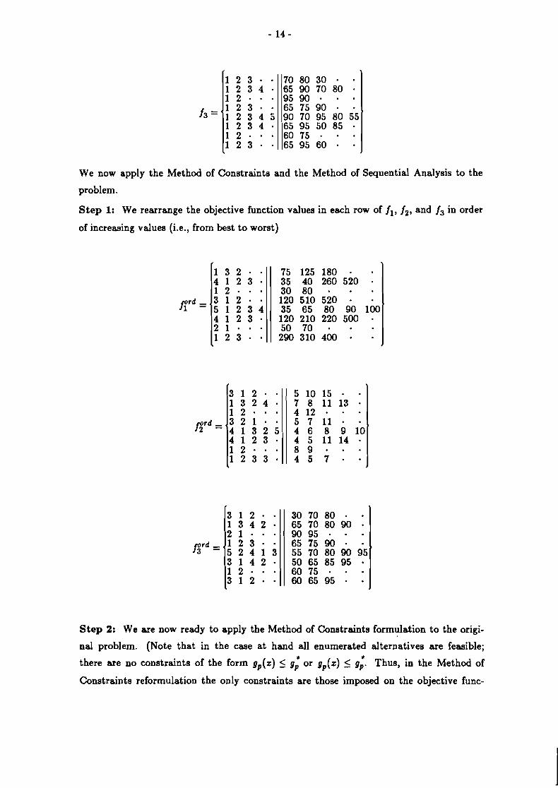
We now apply the Method of Constraints and the Method of Sequential Analysis to the

problem.

Step 1: We rearrange the objective function values in each row of ji, j2, and j3 in order

of increasing values (i.e., from best to worst)

Step 2: We are now ready to apply the Method of Constraints formulation to the origi-

nal problem. (Note that in the case at hand all enumerated alternatives are feasible;

there are no constraints of the form gp(z) 5 gi or gp(z) < Thus, in the Method of

Constraints reformulation the only constraints are those imposed on the objective func-

tions. Since all objective functions are being minimized these constraints will take the

form fi(z) 5 fl*(ko). Thus, we must set kg and calculate fl*(ko).

From the ordered sets of objective function component values found in Step 1 we

find the optimal and worst values for each objective function simply by summing the first

and last columns on the right-hand side of each table. Thus,

In applying the Method of Constraints to this problem it is assumed that each objective

function is equally weighted, i.e., pl = p2 = p3. Then for computational convenience we

can set pi = 1 for every i . Arbitrarily, we set khl) = .4 for the first iteration. Then we

calculate

yielding f;(khl)) = 1401, fi (6 ' ) ) = 61, f;(kh1)) = 570.

Step 3: Now the Method of Sequential Analysis is used to eliminate components of set X

which violate the conditions imposed by the Method of Constraints, i.e.,

For each term in each objective function we calculate f/J)*(khh)), the cut-off value for the

j-th term of the i-th objective function. In effect this cut-off value says, "Suppose all oth-

er terms of the i-th objective function were at their minimal value, what is the highest

value that the j-th term of the i-th objective could assume before the objective violates

conditions". In the problem at hand, calculations are shown below for

fij)*(khl)) = f:(.4) - 2 fi(zfi)pl) for every j = 1, ..., 8, i = 1,2,3

? f

These are the cut-off values for each term of each objective function. Comparing these

cut-off values to the objective function component values themselves are shown in

Table: Cut-Off Levels for t h e

Terms of the Objective Funct ion

fprd, i = 1,2,3, we see that no objective term exceeds its cut-off.

Step 4: We reduce t o , recalculate ( (ko ) as in Step 2, and then repeat the procedure in

Step 3. Letting kA2) = 1/2 ( .4 ) = .2, we find that f i (kh2)) = 1078, f i (kh2)) = 51, f i (kh2)) = 523. Our new table of objective function component cut-off values

is

Using these cut-off values the following vector component values turn out to violate the

given elimination principles:

For d J ) *(0,2)-

For AJ) *(0,2)-

none

For dJ)*(0,2)-

Eliminating these vector term values from set X we find

Step 5: As a result of the elimination process performed in the previous step the table of

criteria values for f3 is now

Notice that in the fourth and sixth rows the lowest attainable objective function

component values have increased due t o the elimination of vector value components

Z41,242, and z63. As a result now fi(2) = 5 1 5 . Therefore, without changing

fj(kh2)) = 523 we can recalculate the table of cut-off values d ~ ) * ( 0 , 2 ) for the third objec-

tive function.

Using these cut-off values the following vector component values are eliminated:

zll, 222, 224, 251, 252, 254, zg2, 264, 272, z 8 ~ . Eliminating these values from set ~ ( ~ 1 , we

are left with the following set of vector component values

Step 6: The ordered tables of criteria values for all three objective functions are now:

Without changing fif(ki2)) = 1078 or f;(ko(2)) = 51, we can now recalculate the

cut-off values for the first and second objective functions as we did in the previous step for

the third objective function. The new optimal objective function component values are

fi(3) = 920 and $(3) = 48 and objective function component cut-off values are:

These cut-off values eliminate one vector component value 232 as a result of the violation

of the elimination principle for AJ)' (0,2)-

232 ; h(z32) = 12 4 fi3)*(0,2) = 7

Thus, the set X of remaining vector component values is

Step 7: With the elimination of vector component value u32 we can once again recalcu-

late cut-off values for the third objective function since now f3f(kA2)) = 520 and the table

of objective function cut-off values Aj)*(0,2) is:

I f in* ( 0 ) 2 )

Vector component value zgl is eliminated for violating condition

f 3 ( zg l ) = 6 5 5 f i8) ' (0,2) = 6 3 .

We are left with a single variant z * = (213) z 2 ~ , 231, 243) 255) 261 271, zg3) which is

the best compromise solution with f l ( z * ) = 1030, f 2 ( z L ) = 51 , f3(z1) = 520, and

4. Computational Experience in Application of Method of Constraints to In-

teger Multi-Objective Problem [I]

Using FORTRAN Dargeiko wrote a standard Method of Constraints algorithm for

the Soviet BESM-6 computer running under the 'Dubna' operating system. The program

was capable of solving in operating memory a problem of dimension n x 1 x M 5 3000,

where

n = number of variables

1 = local number of elements in sets Xi, j = I ,..., n (Xi is the set of alternative

values for the j-th term of vector z )

M = number of criteria

The initial data for the experimental runs was produced by a pseuderandom number gen-

erator whose output was uniformly distributed on an interval (A,B).By varying the

bounds of interval (A,B), criteria values were generated for all n x I elements. Table 1.

shows how to determine the type and number of computational operations performed at

each iteration. Table 2. reproduces the results of Dargeiko's experiments for equally

weighted criteria.

Dargeiko also performed experiments to analyze the impact of varying criteria

weights on the speed with which a solution was found. Thus, problem 2 in Table 1.4 was

solved for three different combinations of criteria weights. For the three sets of weights,

the size of the set of candidate variants was reduced from 501° to 810, 530, 120 respective-

ly after 9, 15, and 12 iterations on ko. In all three cases Dargeiko reports that the compu-

tational time did not exceed a minute.

Table 1.: Computat ional Operations Per formed by

Method of Constraints A lgor i thm for

Integer Mult i-Objective Programming Problems

Number of Operations in a Single Iteration

Addition : n x M Division: 1

Subtraction: n x M Multiplication: M Permutations: n x 1 x M Comparisons: n x 1 x M

Volume of Memory Used Each Iteration: On the order of n x I x M

Tab le 2.: Computat ional Experience w i th Me thod of Const ra in ts

Integer Multi-Objective Programming Problems

REFERENCES

Problem Number

[I] Mikhalevich, V.S., and Volkovich, V.L. (1982) Vychislitel'nyi metod issledovaniya i

proektirovaniya slodnykh sistem. (Computational method for research and design of

complex systems.) Moscow: Nauka.

[2] Mikhalevich, V.S. (1965a) Sequential Optimization Algorithms and Their Applica-

tion. Part 1. Cybernetics 8, no. 5: 851-855.

5

100

5

5

51°0

1580

7

71

[3] Mikhalevich, V.S. (1965b) Sequential Optimization Algorithms and Their Applica-

tion. Part 2. Cybernetics 1, no. 2: 87-92.

n = Number of Variables

1 = Elements in Set U,,j=l, ..., n

M = Number of Criteria

General Number of Variants

Number of Variants after

Elimination Procedure

Number of Iterations on ko

Solution Time (in seconds)

[4] Mikhalevich, V.S., and Shor, N.Z. (19628) Chislennoe reshenie mnogovariantnykh

zadach po metodu posledovatel'nogo analiza variantov. (Numerical solution of mul-

tivariant problems by the method of sequential analysis of variants.) Nauchno-

metododicheekie materialy ekonomiko-matematichedogo eeminara. Vypuck 1. Mos-

3

10

50

50

50''

130

6

68

4

50

10

10

lo50

2500

6

86

1

7

100

100

l0l4

6

11

23

2

10

50

50

50''

80

14

46

cow: LEMM Akademii nauk SSSR. n.p.

[5] Mikhalevich, V.S., and Shor, N.Z. (1962b) 0 chislennykhmetodakh resheniya m n e

govariantnykh planovykh i tekhnikeekonomicheskikh zadach. (Numerical methods

for solving multivariant planning and techniceeconomical problems). Nauchno-

metododicheskie materialy ekonomiko-matematicheskogo seminara V T s Akademii

nauk USSR no. 1: 15-42.

[6] Volkovich, V.L., and Dargeiko, V.F. (1976) A Method of Constraints in Vector O p

timization Problems. Soviet Automatic Control no. 3: 10-13.

[7] Volkovich, V.L., and Dargeiko, V.F. (1972) On an Algorithm of Choosing a

Compromise Solution for Linear Criteria. Cybernetics 8, no. 5: 851-855.

[8] Volkovich, V.L., and Voloshin, V.L. (1978) A Scheme of the Method of Sequential

Analysis and Sifting of Variables. Cybernetics 14, no. 4: 585-593.