problems in data structures and algorithms · tion of the programming problem which appeared in...

2Problems in Data Structures

and Algorithms

Robert E. TarjanPrinceton University and Hewlett Packard

1. Introduction

I would like to talk about various problems I have worked on over the course of mycareer. In this lecture I’ll review simple problems with interesting applications, andproblems that have rich, sometimes surprising, structure.

Let me start by saying a few words about how I view the process of research,discovery and development. (See Figure 1.)

My view is based on my experience with data structures and algorithms in computerscience, but I think it applies more generally. There is an interesting interplay betweentheory and practice. The way I like to work is to start out with some application from thereal world. The real world, of course, is very messy and the application gets modeledor abstracted away into some problem or some setting that someone with a theoreticalbackground can actually deal with. Given the abstraction, I then try to develop a solutionwhich is usually, in the case of computer science, an algorithm, a computational methodto perform some task. We may be able to prove things about the algorithm, its runningtime, its efficiency, and so on. And then, if it’s at all useful, we want to apply thealgorithm back to the application and see if it actually solves the real problem. Thereis an interplay in the experimental domain between the algorithm developed, basedon the abstraction, and the application; perhaps we discover that the abstraction doesnot capture the right parts of the problem; we have solved an interesting mathematicalproblem but it doesn’t solve the real-world application. Then we need to go back andchange the abstraction and solve the new abstract problem and then try to apply thatin practice. In this entire process we are developing a body of new theory and practicewhich can then be used in other settings.

A very interesting and important aspect of computation is that often the key toperforming computations efficiently is to understand the problem, to represent the

18 Robert E. Tarjan

The Discovery/DevelopmentProcess

The Discovery/DevelopmentProcess

Application

Algorithm

experiment

apply

develop

Application

Algorithm

experimentmodel

Abstraction

Old/NewTheory/Process

Figure 1.

problem data appropriately, and to look at the operations that need to be performed onthe data. In this way many algorithmic problems turn into data manipulation problems,and the key issue is to develop the right kind of data structure to solve the problem. Iwould like to talk about several such problems. The real question is to devise a datastructure, or to analyze a data structure which is a concrete representation of some kindof algorithmic process.

2. Optimum Stack Generation Problem

Let’s take a look at the following simple problem. I’ve chosen this problem becauseit’s an abstraction which is, on the one hand, very easy to state, but on the other hand,captures a number of ideas. We are given a finite alphabet �, and a stack S. We wouldlike to generate strings of letters over the alphabet using the stack. There are three stackoperations we can perform.

push (A)—push the letter A from the alphabet onto the stack,emit—output the top letter from the stack,pop—pop the top letter from the stack.

We can perform any sequence of these operations subject to the following well-formedness constraints: we begin with an empty stack, we perform an arbitrary seriesof push, emit and pop operations, we never perform pop from an empty stack, and we

Problems in Data Structures and Algorithms 19

end up with an empty stack. These operations generate some sequence of letters overthe alphabet.

Problem 2.1 Given some string σ over the alphabet, find a minimum length sequenceof stack operations to generate σ .

We would like to find a fast algorithm to find the minimum length sequence ofstack operations for generating any particular string.

For example, consider the string A B C A C B A. We could generate it by per-forming: push (A), emit A, pop A, push (B), emit B, pop B, push (C), emit C, popC etc., but since we have repeated letters in the string we can use the same item onthe stack to generate repeats. A shorter sequence of operations is: push (A), emit A,push (B), emit B, push (C), emit C, push (A), emit A, pop A; now we can emit C (wedon’t have to put a new C on the stack), pop C, emit B, pop B, emit A. We got the‘CBA’ string without having to do additional push-pops. This problem is a simplifica-tion of the programming problem which appeared in “The International Conference onFunctional Programming” in 2001 [46] which calls for optimum parsing of HTML-likeexpressions.

What can we say about this problem? There is an obvious O(n3) dynamic pro-gramming algorithm1. This is really a special case of optimum context-free languageparsing, in which there is a cost associated with each rule, and the goal is to find aminimum-cost parse. For an alphabet of size three there is an O(n) algorithm (Y. Zhou,private communication, 2002). For an alphabet of size four, there is an O(n2) algo-rithm. That is all I know about this problem. I suspect this problem can be solved bymatrix multiplication, which would give a time complexity of O(nα), where α is thebest exponent for matrix multiplication, currently 2.376 [8]. I have no idea whetherthe problem can be solved in O(n2) or in O(n log n) time. Solving this problem, orgetting a better upper bound, or a better lower bound, would reveal more informationabout context-free parsing than what we currently know. I think this kind of questionactually arises in practice. There are also string questions in biology that are related tothis problem.

3. Path Compression

Let me turn to an old, seemingly simple problem with a surprising solution. Theanswer to this problem has already come up several times in some of the talks in

1 Sketch of the algorithm: Let S[1 . . . n] denote the sequence of characters. Note that there must be exactly nemits and that the number of pushes must equal the number of pops. Thus we may assume that the cost is sim-ply the number of pushes. The dynamic programming algorithm is based on the observation that if the samestack item is used to produce, say, S[i1] and S[i2], where i2 > i1 and S[i1] = S[i2], then the state of the stackat the time of emit S[i1] must be restored for emit S[i2]. Thus the cost C[i, j] of producing the subsequenceS[i, j] is the minimum of C[i, j − 1] + 1 and min {C[i, t] + C[t + 1, j − 1] : S[t] = S[ j], i ≤ t < j}.

20 Robert E. Tarjan

the conference “Second Haifa Workshop on Interdisciplinary Applications of GraphTheory, Combinatorics and Algorithms.” The goal is to maintain a collection of nelements that are partitioned into sets, i.e., the sets are always disjoint and each elementis in a unique set. Initially each element is in a singleton set. Each set is named by somearbitrary element in it. We would like to perform the following two operations:

find(x)—for a given arbitrary element x, we want to return the name of the setcontaining it.

unite(x,y)—combine the two sets named by x and y. The new set gets the name ofone of the old sets.

Let’s assume that the number of elements is n. Initially, each element is in a singletonset, and after n − 1 unite operations all the elements are combined into a single set.

Problem 3.1 Find a data structure that minimizes the worst-case total cost of m findoperations intermingled with n − 1 unite operations.

For simplicity in stating time bounds, I assume that m ≥ n, although this assump-tion is not very important. This problem originally arose in the processing of COMMONand EQUIVALENCE statements in the ancient programming language FORTRAN. Asolution is also needed to implement Kruskal’s [ 31] minimum spanning tree algorithm.(See Section 7.)

There is a beautiful and very simple algorithm for solving Problem 3.1, developedin the ‘60s. I’m sure that many of you are familiar with it. We use a forest data structure,with essentially the simplest possible representation of each tree (see Figure 2). We userooted trees, in which each node has one pointer, to its parent. Each set is representedby a tree, whose nodes represent the elements, one element per node. The root elementis the set name. To answer a find(x) operation, we start at the given node x and follow

A

B D F

EC

Figure 2.


C

A

B

D

E

F

Figure 3.

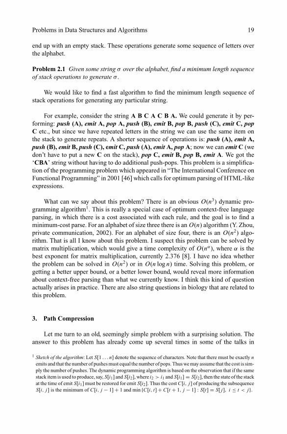
the pointers to the root node, which names the set. The time of the find operation isproportional to the length of the path. The tree structure is important here because itaffects the length of the find path. To perform a unite(x,y) operation, we access the twocorresponding tree roots x and y, and make one of the roots point to the other root. Theunite operation takes constant time.

The question is, how long can find paths be? Well, if this is all there is to it, wecan get bad examples. In particular, we can construct the example in Figure 3: a treewhich is just a long path. If we do lots of finds, each of linear cost, then the total costis proportional to the number of finds times the number of elements, O(m · n), whichis not a happy situation.

As we know, there are a couple of heuristics we can add to this method to sub-stantially improve the running time. We use the fact that the structure of each tree iscompletely arbitrary. The best structure for the finds would be if each tree has all itsnodes just one step away from the root. Then find operations would all be at constantcost. But as we do the unite operations, depths of nodes grow. If we perform the unitesintelligently, however, we can ensure that depths do not become too big. I shall givetwo methods for doing this.

Unite by size (Galler and Fischer [16]): This method combines two trees into one bymaking the root of the smaller tree point to the root of the larger tree (breaking a tiearbitrarily). The method is described in the pseudo-code below. We maintain with eachroot x the tree size, size(x) (the number of nodes in the tree).

22 Robert E. Tarjan

unite(x,y): If size (x) ≥ size (y) make x the parent of y and set

size (x) ← size (x) + size (y)

Otherwise make y the parent of x and set

size (y) ← size (x) + size (y)

Unite by rank (Tarjan and van Leewen [41]): In this method each root contains a rank,which is an estimate of the depth of the tree. To combine two trees with roots of differentrank, we attach the tree whose root has smaller rank to the other tree, without changingany ranks. To combine two trees with roots of the same rank, we attach either tree tothe other, and increase the rank of the new root by one. The pseudo code is below. Wemaintain with each root x its rank, rank(x). Initially, the rank of each node is zero.

unite(x, y): if rank (x) > rank (y) make x the parent of y else

if rank (x) < rank (y) make y the parent of x else

if rank (x) = rank (y) make x the parent of y and increase the rank of xby 1.

Use of either of the rules above improves the complexity drastically. In particular,the worst-case find time decreases from linear to logarithmic. Now the total cost fora sequence of m find operations and n − 1 intermixed unite operations is (m log n),because with either rule the depth of a tree is logarithmic in its size. This result (forunion by size) is in [16].

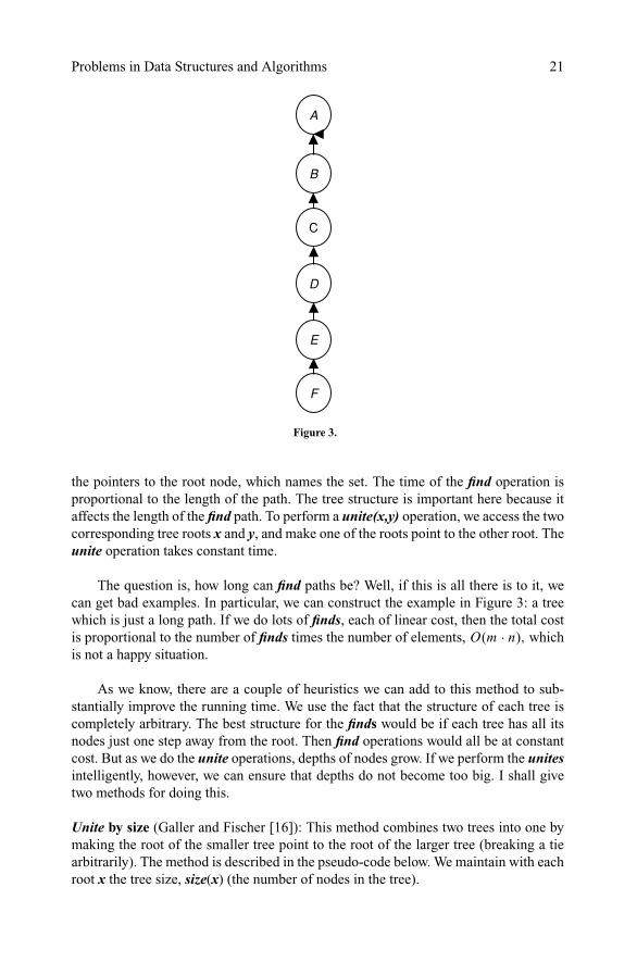
There is one more thing we can do to improve the complexity of the solution toProblem 3.1. It is an idea that Knuth [29] attributes to Alan Tritter, and Hopcroft andUllman [20] attribute to McIlroy and Morris. The idea is to modify the trees not onlywhen we do unite operations, but also when we do find operations: when doing a find,we “squash” the tree along the find path. (See Figure 4.) When we perform a find onan element, say E, we walk up the path to the root, A, which is the name of the setrepresented by this tree. We now know not only the answer for E, but also the answerfor every node along the path from E to the root. We take advantage of this fact bycompressing this path, making all nodes on it point directly to the root. The tree ismodified as depicted in Figure 4. Thus, if later we do a find on say, D, this node is nowone step away from it the root, instead of three steps away.

The question is, by how much does path compression improve the speed of thealgorithm? Analyzing this algorithm, especially if both path compression and one ofthe unite rules is used, is complicated, and Knuth proposed it as a challenge. Note thatif both path compression and union by rank are used, then the rank of tree root is notnecessarily the tree height, but it is always an upper bound on the tree height. Let meremind you of the history of the bounds on this problem from the early 1970’s.

There was an early incorrect “proof” of an O(m) time-bound; that is, constanttime per find. Shortly thereafter, Mike Fischer [11] obtained a correct bound of


A

B

C

D

E

E D C B

A

Figure 4.

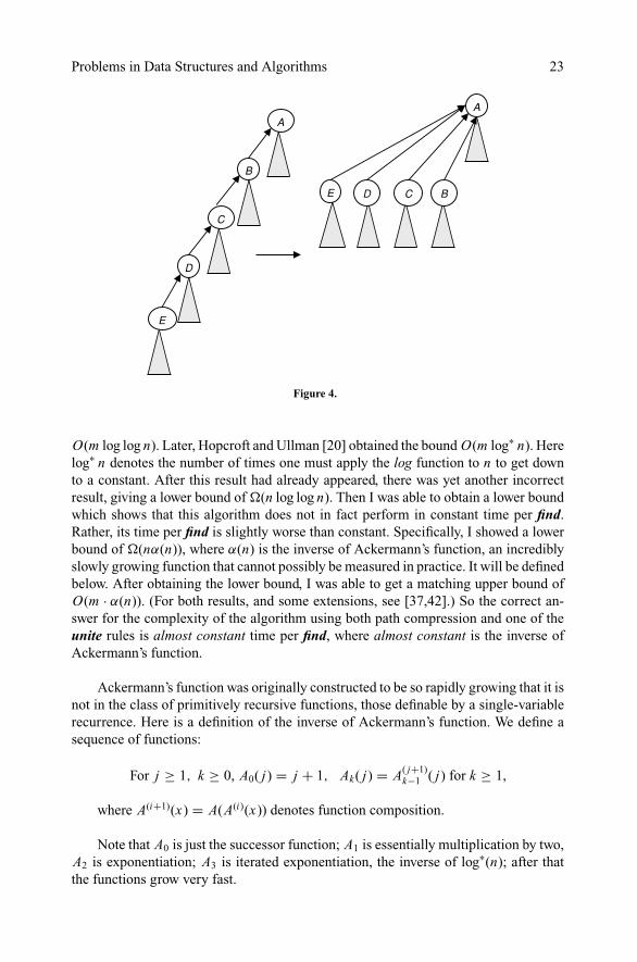
O(m log log n). Later, Hopcroft and Ullman [20] obtained the bound O(m log∗ n). Herelog∗ n denotes the number of times one must apply the log function to n to get downto a constant. After this result had already appeared, there was yet another incorrectresult, giving a lower bound of (n log log n). Then I was able to obtain a lower boundwhich shows that this algorithm does not in fact perform in constant time per find.Rather, its time per find is slightly worse than constant. Specifically, I showed a lowerbound of (nα(n)), where α(n) is the inverse of Ackermann’s function, an incrediblyslowly growing function that cannot possibly be measured in practice. It will be definedbelow. After obtaining the lower bound, I was able to get a matching upper bound ofO(m · α(n)). (For both results, and some extensions, see [37,42].) So the correct an-swer for the complexity of the algorithm using both path compression and one of theunite rules is almost constant time per find, where almost constant is the inverse ofAckermann’s function.

Ackermann’s function was originally constructed to be so rapidly growing that it isnot in the class of primitively recursive functions, those definable by a single-variablerecurrence. Here is a definition of the inverse of Ackermann’s function. We define asequence of functions:

For j ≥ 1, k ≥ 0, A0( j) = j + 1, Ak( j) = A( j+1)k−1 ( j) for k ≥ 1,

where A(i+1)(x) = A(A(i)(x)) denotes function composition.

Note that A0 is just the successor function; A1 is essentially multiplication by two,A2 is exponentiation; A3 is iterated exponentiation, the inverse of log∗(n); after thatthe functions grow very fast.

24 Robert E. Tarjan

The inverse of Ackermann’s function is defined as:

α(n) = min {k : Ak(1) ≥ n}

The growth of the function α(n) is incredibly slow. The smallest n such that α(n) =4 for example, is greater than any size of any problem that anyone will ever solve, inthe course of all time.

The most interesting thing about this problem is the surprising emergence of α(n)in the time bound. I was able to obtain such a bound because I guessed that the truth wasthat the time per find is not constant (and I was right). Given this guess, I was able toconstruct a sequence of bad examples defined using a double recursion, which naturallyled to Ackermann’s function. Since I obtained this result, the inverse of Ackermann’sfunction has turned up in a number of other places in computer science, especially incomputational geometry, in bounding the complexity of various geometrical configu-rations involving lines and points and other objects [34].

Let one mention some further work on this problem. The tree data structure forrepresenting sets, though simple, is very powerful. One can attach values to the edges ornodes of the trees and combine values along tree paths using find. This idea has manyapplications [39]. There are variants of path compression that have the same inverseAckermann function bound and some other variants that have worse bounds [42]. Thelower bound that I originally obtained was for the particular algorithm that I havedescribed. But the inverse Ackermann function turns out to be inherent in the problem.There is no way to solve the problem without having the inverse Ackermann functiondependence. I was able to show this for a pointer machine computation model withcertain restrictions [38]. Later Fredman and Saks [12] showed this for the cell probecomputation model; theirs is a really beautiful result. Recently, Haim Kaplan, NiraShafrir and I [24] have extended the data structure to support insertions and deletionsof elements.

4. Amortization and Self-adjusting Search Trees

The analysis of path compression that leads to the inverse Ackermann function is com-plicated. But it illustrates a very important concept, which is the notion of amortization.The algorithm for Problem 3.1 performs a sequence of intermixed unite and find op-erations. Such operations can in fact produce a deep tree, causing at least one findoperation to take logarithmic time. But such a find operation squashes the tree andcauses later finds to be cheap. Since we are interested in measuring the total cost, wedo not mind if some operations are expensive, as long as they are balanced by cheapones. This leads to the notion of amortizatized cost, which is the cost per operationaveraged over a worst-case sequence of operations. Problem 3.1 is the first examplethat I am aware of where this notion arose, although in the original work on the problemthe word amortization was not used and the framework used nowadays for doing anamortized analysis was unknown then. The idea of a data structure in which simple


modifications improve things for later operations is extremely powerful. I would like toturn to another data structure in which this idea comes into play—self-adjusting searchtrees.

4.1. Search Trees

There is a type of self-adjusting search tree called the splay tree that I’m sure manyof you know about. It was invented by Danny Sleater and me [35]. As we shall see, manycomplexity results are known for splay trees; these results rely on some clever ideasin algorithmic analysis. But the ultimate question of whether the splaying algorithm isoptimal to within a constant factor remains an open problem.

Let me remind you about binary search trees.

Definition 4.1 A binary search tree is a binary tree, (every node has a left and a rightchild, either of which, or both, can be missing.) Each node contains a distinct item ofdata. The items are selected from a totally ordered universe. The items are arranged inthe binary search tree in the following way: for every node x in the tree, every node inthe left subtree of x is less than the item stored in x and every node in the right subtreeof x is greater than the item stored in x The operations done on the tree are access,insert and delete.

We perform an access of an item in the obvious way: we start at the root, and we godown the tree, choosing at every node whether to go left or right by comparing the itemin the node with the item we trying to find. The search time is proportional to the depthof the tree or, more precisely, the length of the path from the root to the designateditem. For example, in Figure 5, a search for “frog”, which is at the root, takes one step;a search for “zebra”, takes four steps. Searching for “zebra” is more expensive, but nottoo expensive, because the tree is reasonably balanced. Of course, there are “bad” trees,such as long paths, and there are “good” trees, which are spread out wide like the onein Figure 5. If we have a fixed set of items, it is easy to construct a perfectly balancedtree, which gives us logarithmic worst-case access time.

frog

cow

dogcat

horse

goat

pig

rabbit

zebra

Figure 5.

26 Robert E. Tarjan

The situation becomes more interesting if we want to allow insertion and deletionoperations, since the shape of the tree will change. There are standard methods forinserting and deleting items in a binary search tree. Let me remind you how these work.The easiest method for an insert operation is just to follow the search path, which willrun off the bottom of the tree, and put the new item in a new node attached wherethe search exits the tree. A delete operation is slightly more complicated. Consider thetree in Figure 5. If I want to delete say “pig” (a leaf in the tree in Figure 5), I simplydelete the node containing it. But if I want to delete “frog”, which is at the root, I haveto replace that node with another node. I can get the replacement node by taking theleft branch from the root and then going all the way down to the right, giving me thepredecessor of “frog”, which happens to be “dog”, and moving it to replace the root. Or,symmetrically, I can take the successor of “frog” and move it to the position of “frog”.In either case, the node used to replace frog has no children, so it can be moved withoutfurther changes to the tree. Such a replacement node can actually have one child (butnot two); after moving such a node, we must replace it with its child. In any case, aninsertion or deletion takes essentially one search in the tree plus a constant amount ofrestructuring. The time spent is at most proportional to the tree depth.

Insertion and deletion change the tree structure. Indeed, a bad sequence of suchoperations can create an unbalanced tree, in which accesses are expensive. To remedythis we need to restructure the tree somehow, to restore it to a “good” state.

The standard operation for restructuring trees is the rebalancing operation calledrotation. A rotation takes an edge such as ( f, k) in the tree in Figure 6 and switches itaround to become (k, f ). The operation shown is a right rotation; the inverse operationis a left rotation. In a standard computer representation of a search tree, a rotation takesconstant time; the resulting tree is still a binary search tree for the same set of ordereditems. Rotation is universal in the sense that any tree on some set of ordered items canbe turned into any other tree on the same set of ordered items by doing an appropriatesequence of rotations.

k

f

f

k

BA

C

CB

A

right

left

Figure 6.


We can use rotations to rebalance a tree when insertions and deletions occur. Thereare various “balanced tree” structures that use extra information to determine whatrotations must be done to restore balance during insertions and deletions. Examplesinclude AVL trees [1], red-black trees [19,40], and many others. All these balancedtree structures have the property that the worst-case time for a search, insertion ordeletion in an n-node tree is O(log n).

4.2. Splay Trees

This is not the end of the story, because balanced search trees have certaindrawbacks:

� Extra space is needed to keep track of the balance information.� The rebalancing needed for insertions and deletions involves several cases, and

can be complicated.� Perhaps most important, the data structure is logarithmic-worst-case but essen-

tially logarithmic-best-case as well. The structure is not optimum for a non-uniform usage pattern. Suppose for example I have a tree with a million itemsbut I only access a thousand of them. I would like the thousand items to becheap to access, proportional to log (1,000), not to log (1,000,000). A standardbalanced search tree does not provide this.

There are various data structures that have been invented to handle this last draw-back. Assume that we know something about the usage pattern. For example, supposewe have an estimate of the access frequency for each item. Then we can constructan “optimum” search tree, which minimizes the average access time. But what if theaccess pattern changes over time? This happens often in practice.

Motivated by this issue and knowing about the amortized bound for path compres-sion, Danny Sleator and I considered the following problem:

Problem 4.2 Is there a simple, self-adjusting form of search tree that does not need anexplicit balance condition but takes advantage of the usage pattern? That is, is therean update mechanism that adjusts the tree automatically, based on the way it is used?

The goal is to have items that are accessed more frequently move up in the tree,and items that are accessed less frequently move down in the tree.

We were able to come up with such a structure, which we called the splay tree.A Splay tree is a self-adjusting search tree. See Figure 7 for an artist’s conception of aself-adjusting tree.

“Splay” as a verb means to spread out. Splaying is a simple self-adjusting heuristic,like path compression, but that applies to binary search trees. The splaying heuristictakes a designated item and moves it up to the root of the tree by performing rotations,

28 Robert E. Tarjan

Figure 7.

preserving the item order. The starting point of the idea is to perform rotations bottom-up. It turns out, though, that doing rotations one at a time, in strict bottom-up order,does not produce good behavior. The splay heuristic performs rotations in pairs, inbottom-up order, according to the rules shown in Figure 8 and explained below. Toaccess an item, we walk down the tree until reaching the item, and then perform thesplay operation, which moves the item all the way up to the tree root. Every item alongthe search path has its distance to the root roughly halved, and all other nodes get pushedto the side. No node moves down more than a constant number of steps.


Cases of splaying

A

B C

y

x

ZIg

y

A

C

B

x

Zig-Zigy

A

C

B

x

z

D

y

C

B

D

z

x

A

Z

A

D

B

Y

X

C

X

A DB

Y Z

C

Zig-Zag

(c)

(b)

(a)

Figure 8.

Figure 8 shows the cases of a single splaying step. Assume x is the node to beaccessed. If the two edges above x toward the root are in the same direction, we do arotation on the top edge first and then on the bottom edge, which locally transformsthe tree as seen in Figure 7b. This transformation doesn’t look helpful; but in fact,when a sequence of such steps are performed, they have a positive effect. This is the“zig-zig” case. If the two edges from x toward the root are in opposite directions, suchas right-left as seen in Figure 8c, or symmetrically left-right, then the bottom rotationis done first, followed by the top rotation. In this case, x moves up and y and z get splitbetween the two subtrees of x . This is the zig-zag case. We keep doing zig-zag and

30 Robert E. Tarjan

6 6 6

6

6

666

5 5

5 5

5555

4 4 4 4

44

44

3

3

3 3

3

3

3

3

2 2

2 2

2

22

2

1

1

1

1

1

1

11

Pare zig zag

Pare zig zag

(a)

(b)

Figure 9.

zig-zig steps, as appropriate, moving x up two steps at a time, until either x is the rootor it is one step away from the root. In the latter case we then do one final rotation,the zig case (Figure 8a). The splay operation is an entire sequence of splay steps thatmoves a designated item all the way up to the root.

Figure 9a contains a step-by-step example of a complete splay operation. This isa purely zig-zig case (except for a final zig). First we perform two rotations, movingitem #1 up the path, and then two more rotations, moving item #1 further up thepath. Finally, a last rotation is performed to make item #1 take root. Transforming theinitial configuration into the final one is called “splaying at node 1 ”. Figure 9b givesa step-by-step example of a purely zig-zag case.

Figure 10 is another example of a purely zig-zag case of a single splay operation.The accessed node moves to the root, every other node along the find path has itsdistance to the root roughly halved, and no nodes are pushed down by more thana constant amount. If we start out with a really bad example, and we do a numberof splay operations, the tree gets balanced very quickly. The splay operation can beused not only during accesses but also as the basis of simple and efficient insertions,deletions, and other operations on search trees.

There is also a top-down version of splaying as well as other variants [35]. Sleatorhas posted code for the top-down version at [47].


1

2

3

4

5

6

7

8

9

10

7

8

1

2

3

4

5

9

10

6

Splaying

Figure 10.

4.3. Complexity Results

The main question for us as theoreticians is, “How does this algorithm perform?”Sleator and I were able to show that, in the amortized sense, this algorithm performsjust as well as any balanced tree structure.

Theorem 4.3 Beginning with an arbitrary n-node tree, suppose we perform a sequenceof m accesses and ignore start-up effects; that is, we assume that m ≥ n. The followingresults hold:

(a) The total cost of m accesses is O(m log n), thus matching the bound for bal-anced trees.

(b) The splaying algorithm on any access sequence performs within a constantfactor of the performance of that of the best possible static tree for the givenaccess sequence (in spite of the fact that this algorithm does not know theaccess frequencies ahead of time and doesn’t keep track of them).

(c) If the items are accessed in increasing order, each once, the total access timeis linear. That is, the amortized cost per access is constant, as compared tologarithmic for a balanced search tree or for any static tree. This result demon-strates that modifying the tree as operations proceed can dramatically improvethe access cost in certain situations.

It is relatively straightforward to prove results (a) and (b) above. They follow froman interesting “potential” argument that I trust many of you know. These results can befound in [35], along with additional applications and extensions. Result (c) seems tobe hard to prove — an elaborate inductive argument appears in [41].

The behavior of a splay tree when sequential accesses are performed is quiteinteresting. Suppose we start with an extreme tree that is just a long left path, with thesmallest item at the bottom of the path, and begin accessing the items in increasingorder. The first access costs n. The next access costs about n/2, the next one costs n/4,

and so on. The access time drops by about a factor of two with each access until afterabout logarithmically many accesses, at which time the tree is quite well-balanced.

32 Robert E. Tarjan

Then the time per access starts behaving something like a ruler function, with a certainamount of randomness thrown in: about half the accesses take constant time; about aquarter take about twice as long; about an eighth take about three times as long; andso on. The amortized cost per access is constant rather than logarithmic.

Based on results (a)—(c) and others, Sleator and I made (what we consider to be)an audacious conjecture. Suppose we begin with some n-node search tree and performa sequence of accesses. (For simplicity, we ignore insertions and deletions.) The cost toaccess an item is the number of nodes on the path from the root to the item. At any time,we can perform one or more rotations, at a cost of one per rotation. Then, knowing theentire access sequence ahead of time, there is a pattern of rotations that minimizes thetotal cost of the accesses and the rotations. This is the optimal offline algorithm, forthe given initial tree and the given access sequence.

Problem 4.4 Dynamic Optimality Conjecture: Prove or disprove that for any initialtree and any access sequence, the splaying algorithm comes within a constant factorof the optimal off-line algorithm.

Note that splaying is an on-line algorithm: its behavior is independent of futureaccesses, depending only on the initial tree and the accesses done so far. Furthermorethe only information the algorithm retains about the accesses done so far is implicit inthe current state of the tree. A weaker form of Problem 4.4 asks whether there is anyon-line algorithm whose performance is within a constant factor of that of the optimumoff-line algorithm.

The closest that anyone has come to proving the strong form of the conjecture isan extension by Richard Cole and colleagues of the sequential access result, Theorem4.3(c). Consider a sequence of accesses. For simplicity, assume that the items are 1, 2,3, in the corresponding order. The distance between two items, say i and j , is definedto be | i − j | + 2. Cole et al. proved the following:

Theorem 4.4 [6,7]: The total cost of a sequence of accesses using splaying is at mostof the order of n plus m plus the sum of the logarithms of the distances betweenconsecutively accessed items.

This result, the “dynamic finger theorem”, is a special case of the (strong) dynamicoptimality conjecture. Significant progress on the weak form of the conjecture has beenmade recently by Demaine and colleagues [9]. They have designed an on-line searchtree update algorithm that comes within a loglog performance factor of the optimaloff-line algorithm (as compared to the log factor of a balanced tree algorithm). A keypart of their result is a lower bound on the cost of an access sequence derived byBob Wilber [43]. The algorithm of Demaine et al. is cleverly constructed so that itsperformance comes within a loglog factor of Wilber’s lower bound. They also argue thatuse of Wilber’s lower bound will offer no improvement beyond loglog. An immediatequestion is whether one can prove a similar loglog bound for splaying, even if thedynamic optimality conjecture remains out of reach.


To summarize, we do not know the answer to the following question:

Is the splaying algorithm (or any on-line binary search tree algorithm) optimal to withina constant factor?

Splaying as well as path compression are examples of very simple operations thatgive rise when repeated to complicated, hard-to-analyze, behavior. Splay trees havebeen used in various systems applications, for memory management, table storage, andother things. In many applications of tables, most of the data does not get accessed mostof the time. The splaying tree algorithm takes advantage of such locality of reference:the splay algorithm moves the current working set to the top of the tree, where it isaccessible at low cost. As the working set changes, the new working set moves to thetop of the tree.

The drawback of this data structure is, of course, that it performs rotations all thetime, during accesses as well as during insertions and deletions. Nevertheless, it seemsto work very well in practical situations in which the access pattern is changing.

5. The Rotation Distance between Search Trees

Search trees are a fascinating topic, not just because they are useful data structures,but also because they have interesting mathematical properties. I have mentioned thatany search tree can be transformed into any other search tree on the same set of ordereditems by performing an appropriate sequence of rotations. This fact raises at least twointeresting questions, one algorithmic, one structural.

Problem 5.1 Given two n-node trees, how many rotations does it take to convert onetree into the other?

This question seems to be NP- hard. A related question is how far apart can two treesbe? To formulate the question more precisely, we define the rotation graph on n-nodetrees in the following way: The vertices of the graph are the n-node binary trees. Twotrees are connected by an edge if and only if one tree can be obtained from the otherby doing a single rotation. This graph is connected.

Problem 5.2 What is the diameter of the rotation graph described above as a functionof n?

It is easy to get an upper bound of 2n for the diameter. It is also easy to get a lowerbound of n − O(1), but this leaves a factor of two gap. Sleator and I worked with BillThurston on this problem. He somehow manages to map every possible problem intohyperbolic geometry. Using mostly Thurston’s ideas, we were able to show that the 2nbound is tight, by applying a volumetric argument in hyperbolic space. We were evenable to establish the exact bound for large enough n, which is 2n − 6 [36]. To me thisis an amazing result. The details get quite technical, but this is an example in which a

34 Robert E. Tarjan

piece of mathematics gets brought in from way out in left field to solve a nitty-grittydata structure problem. This just goes to show the power of mathematics in the world.

6. Static Optimum Search Trees

A final question about search trees concerns static optimum trees. Suppose wewant to store n ordered items in a fixed search tree so as to minimize the average accesstime, assuming that each item is accessed independently with a fixed probability, andthat we know the access probabilities. The problem is to construct the best tree. Thereare an exponential number of trees, so it might take exponential time find the best one,but in fact it does not. There are two versions of this problem, depending on the kindof binary search tree we want.

Problem 6.1 Items can be stored in the internal nodes of the tree. (This is the kind ofsearch tree discussed in Sections 4 and 5.)

The problem in this case is: Given positive weights w1, w2, . . . , wn , construct an n-node binary tree that minimizes

∑ni=1 wi di , where di is the depth of the i-th node in

symmetric order.

Problem 6.2 Items can be stored only in the external nodes (the leaves) of the tree.

The problem in this case is: Given positive weights w1, w2, . . . , wn , construct a binarytree with n external nodes that minimizes

∑ni=1 wi di , where di is the depth of the i-th

external node in symmetric order.

Problem 6.1 can be solved by a straightforward O(n3)-time dynamic programmingalgorithm (as in the stack generation problem discussed in Section 2). Knuth[30] wasable to improve on this by showing that there is no need to look at all the subproblems;there is a restriction on the subproblems that have to be considered, which reduces thetime to O(n2). This result was extended by Frances Yao [45] to other problems. Yaocaptured a certain kind of structural restriction that she called “quadrangle inequalities”.Here we have an O(n2) dynamic programming algorithm with a certain amount ofcleverness in it. This result is twenty-five years old or so. Nothing better is known.There may, in fact, be a faster algorithm for Problem 6.1; no nontrivial lower bound forthe problem is known.

For Problem 6.2, in which the items are stored in the external nodes and theinternal nodes just contain values used to support searching, we can do better. Thereis a beautiful algorithm due to Hu and Tucker [21] that runs in O(n log n) time. Thisalgorithm is an extension of the classical algorithm of Huffman [22] for building so-called “Huffman codes”. The difference between Hoffman codes and search trees isthe alphabetic restriction: in a search tree the items have to be in a particular order inthe leaves, whereas in a Huffman code they can be permuted arbitrarily. It turns out that


a simple variant of the Huffman coding algorithm solves Problem 6.2. The amazingthing about this is that the proof of correctness is inordinately complicated. Garsiaand Wachs [17] presented a variant of the algorithm with an arguably simpler proof ofcorrectness, and Karpinski et al. [26] have made further progress on simplifying theproofs of both algorithms. But it is still quite a miracle that these simple algorithmswork. And again, there is no lower bound known. In fact, there is no reason to believethat the problem cannot be solved in linear time, and there is good reason to believethat maybe it can: for some interesting special cases the problem can indeed be solvedin linear time [27].

7. The Minimum Spanning Tree Problem

Let me close by coming back to a classical graph problem—the minimum span-ning tree problem. Given a connected, undirected graph with edge costs, we want tofind a spanning tree of minimum total edge cost. This problem is a classical networkoptimization problem, and it is about the simplest problem in this area. It has a very longhistory, nicely described by Graham and Hell [18]. The first fully-realized algorithmsfor this problem were developed in the 1920’s. There are three classic algorithms. Themost recently discovered is Kruskal’s algorithm [31], with which we are all familiar.This algorithm processes the edges in increasing order by cost, building up the treeedge-by-edge. If a given edge connects two different connected components of whathas been built so far, we add it as an additional edge; if it connects two vertices in thesame component, we throw it away. To implement this algorithm, we need an algorithmto sort (or at least partially sort) the edges, plus a data structure to keep track of thecomponents. Keeping track of the components is exactly the set union problem dis-cussed in Section 3. The running time of Kruskal’s algorithm is O(m log n) includingthe sorting time. If the edges are presorted by cost, the running time of the algorithmis the same as that of disjoint set union; namely, O(m α(n)), where α(n) is the inverseAckermann function.

An earlier algorithm, usually credited to Prim [33] and Dijkstra [10], is a single-source version of Kruskal’s algorithm. It begins with a vertex and grows a tree from it byrepeatedly adding the cheapest edge connecting the tree to a new vertex. This algorithmwas actually discovered by Jarnık in 1930 [23]. It runs in O(n2) time, as implementedby Prim and Dijkstra. (Jarnık did not consider its computational complexity at all.) Byusing a data structure called a heap (or priority queue) the algorithm can be implementedto run in O(m log n) time.

An even earlier algorithm, a beautiful parallel one, was described by Boruvka [3]in 1926. It also has a running time of O(m log n). (The time bound is recent; Boruvkadid not investigate its complexity.) This algorithm is Kruskal’s algorithm in parallel. Inthe first iteration, for every vertex pick the cheapest incident edge and add it the set ofedges so far selected. In general, the chosen edges form a set of trees. As long as thereare at least two such trees, pick the cheapest edge incident to each tree and add these

36 Robert E. Tarjan

edges to the chosen set. In every iteration the number of trees decreases by at least afactor of two, giving a logarithmic bound on the number of iterations. If there are edgesof equal cost, a consistent tie-breaking rule must be used, or the algorithm will createcycles, but this is just a technical detail.

All three classic algorithms run in O(m log n) time if they are implemented ap-propriately. The obvious question is whether sorting is really needed, or can one canget rid of the log factor and solve this problem in linear time? Andy Yao [44] was thefirst to make progress. He added a new idea to Boruvka’s algorithm that reduced therunning time to O(m log log n). He thereby showed that sorting was not, in fact, in-herent in the minimum spanning tree problem. A sequence of improvements followed,all based on Boruvka’s algorithm. Mike Fredman and I [13] achieved a running time ofO(m log∗ n) by using a new data structure called the Fibonacci heap in combinationwith Boruvka’s algorithm. By adding a third idea, that of packets, Galil, Gabor, andSpencer [14] (see also [15]) obtained O(m log log∗ n) running time. Finally, Klein andTarjan [28] (see also [25]) used random sampling in combination with a linear-timealgorithm for verification of minimum spanning trees to reach the ultimate goal, a lineartime algorithm for finding minimum spanning trees.

One may ask whether random sampling is really necessary. Is there a deterministiclinear-time algorithm to find minimum spanning trees? Bernard Chazelle [4,5], in aremarkable tour de force, invented a new data structure, called the soft heap, and usedit to obtain a minimum spanning tree algorithm with a running time of O(m α(n)). (Ourold friend, the inverse Ackermann function, shows up again!) Soft heaps make errors,but only in a controlled way. This idea of allowing controlled errors is reminiscentof the remarkable (and remarkably complicated) O(n log n)-size sorting network ofAijtai, Komlos, and Szemeredi [2], which uses partition sorting with careful controlof errors.

Chazelle’s ideas were used in a different way by Pettie and Ramachandran [32] whodesigned a minimum spanning tree algorithm that has a running time optimum to withina constant factor, but whose running time they could not actually analyze. The extraidea in their construction is that of building an optimum algorithm for very-small-sizesubproblems by exhaustively searching the space of all possible algorithms, and thencombining this algorithm with a fixed-depth recursion based on Chazelle’s approach.

In conclusion, we now know that minimum spanning trees can be found in lineartime using random sampling, and we know an optimum deterministic algorithm but wedon’t know how fast it runs (no slower than O(m α(n)), possibly as fast as O(m)). Thisis the strange unsettled state of the minimum spanning tree problem at the moment.

Acknowledgments

My thanks to Mitra Kelly, Sandra Barreto, and Irith Hartman for their hard workin helping prepare the manuscript.


References

[1] G. M. Adel’son-Vel’skii and E.M. Landis, An algorithm for the organization of information,Soviet Math Dokl. 3: 1259–1262 (1962).

[2] M. Ajtai, J. Komlos, and E. Szemeredi, Sorting in c log n parallel steps, Combinatorica3: 1–19 (1983).

[3] O. Boruvka, O jistem problemu minimalnım, Prace Mor. Pr ıroved. Spol. v Brne (ActaSociet. Scient. Natur. Moravicae) 3: 37–58 (1926).

[4] B. Chazelle, The soft heap: an approximate priority queue with optimal error rate,J. Assoc. Comput. Mach. 47: 1012–1027 (2000).

[5] B. Chazelle, A minimum spanning tree algorithm with inverse-Ackermann type complexity,J. Assoc. Comput. Mach. 47: 1028–1047 (2000).

[6] R. Cole, B. Mishra, J. Schmidt, and A. Siegel, On the dynamic finger conjecturefor splay trees, part I: splay sorting logn -block sequences, SIAM J. Computing 30:1–43 (2000).

[7] R. Cole, On the dynamic finger conjecture for splay trees, part II: the proof, SIAM J.Computing 30: 44–85 (2000).

[8] D. Coppersmith and S. Winograd, Matrix multiplication via arithmetic progressions,J. Symbolic Computation 9: 251–280 (1990).

[9] E. D. Demaine, D. Harmon, J. Iacono, and M. Patrascu, Dynamic optimality—almost, Proc45thAnnual IEEE Symp. on Foundations of Computer Science, (2004) pp. 484–490.

[10] E. W. Dijkstra, A note on two problems in connexion with graphs, Num. Mathematik 1:269–271 (1959).

[11] M. J. Fischer, Efficiency of equivalence algorithms, Complexity of Computer Compu-tations, R. E. Miller and J. W. Thatcher, eds., Plenum Press, New York, NY, (1972)pp. 153–168.

[12] M. L. Fredman and M. E. Saks, The cell probe complexity of dynamic data structures, Proc.21st Annual ACM Symp. on Theory of Computing, (1989) pp. 345–354.

[13] M. R. Fredman and R. E. Tarjan, Fibonacci heaps and their uses in improved networkoptimization algorithms, J. Assoc. Comput. Mach. 34: 596–615 (1987).

[14] H. N. Gabow, Z. Galil, and T. H. Spencer, Efficient implementation of graph algo-rithms using contraction, Proc. 25thAnnual IEEE Symp. on Found. of Comp. Sci., (1984)pp. 347–357.

[15] H. N. Gabow, Z. Galil, T. Spencer, and R. E. Tarjan, Efficient algorithms for findingminimum spanning trees in directed and undirected graphs, Combinatorica 6: 109–122(1986).

38 Robert E. Tarjan

[16] B. A. Galler and M. J. Fischer, An improved equivalence algorithm, Comm. Assoc. Comput.Mach. 7: 301–303 (1964).

[17] A. M. Garsia and M. L. Wachs, A new algorithm for minimal binary encodings, SIAM J.Comput. 6: 622–642 (1977).

[18] R. L. Graham and P. Hell, On the history of the minimum spanning tree problem, Annualsof the History of Computing 7: 43–57 (1985).

[19] L. J. Guibas and R. Sedgewick, A dichromatic framework for balanced trees, Proc. 19th

Annual IEEE Symp. on Foundations of Computer Science, (1978) pp. 8–21.

[20] J. Hopcroft and J. D. Ullman, Set-merging algorithms, SIAM J. Comput. 2: 294–303 (1973).

[21] T. C. Hu and A. C. Tucker, Optimal computer search trees and variable-length alphabeticcodes, SIAM J. Appl. Math 21: 514–532 (1971).

[22] D. A. Huffman, A method for the construction of minimum-redundancy codes, Proc. IRE40: 1098–1101 (1952).

[23] V. Jarnık, O jistem problemu minimalnım, Prace Mor. Prıroved. Spol. v Brne (Acta Societ.Scient. Natur. Moraricae) 6: 57–63 (1930).

[24] H. Kaplan, N. Shafrir, and R. E. Tarjan, Union-find with deletions, Proc. 13th AnnualACM-SIAM Symp. on Discrete Algorithms, (2002) pp. 19–28.

[25] D. R. Karger, P. N. Klein, and R. E. Tarjan, A randomized linear-time algorithm to findminimum spanning trees, J. Assoc. Comput. Mach. 42: 321–328 (1995).

[26] M. Karpinski, L. L. Larmore, and V. Rytter, Correctness of constructing optimal alphabetictrees revisited, Theoretical Computer Science 180: 309–324 (1997).

[27] M. Klawe and B. Mumey, Upper and lower bounds on constructing alphabetic binary trees,Proc 4 thAnnual ACM-SIAM Symp. on Discrete Algorithms, (1993) pp. 185–193.

[28] P. N. Klein and R. E. Tarjan, A randomized linear-time algorithm for finding minimumspanning trees, Proc. 26 thAnnual ACM Symp. on Theory of Computing, (1994) pp. 9–15.

[29] D. E. Knuth, The Art of Computer Programming, Vol. 1: Fundamental Algorithms, SecondEdition, Addison-Wesley, Reading, MA, (1973) p. 572.

[30] D. E. Knuth, Optimum binary search trees, Acta Informatica 1: 14–25 (1971).

[31] J. B. Kruskal, On the shortest spannng subtree of a graph and the travelling saleman problem,Proc. Amer. Math. Soc. 7: 48–50 (1956).

[32] S. Pettie and V. Ramachandran, An optimal minimum spanning tree algorithm, J. Assoc.Comput. Mach. 49: 16–34 (2002).


[33] R. C. Prim, The shortest connecting network and some generalizations, Bell Syst. Tech. J.36: 1389–1401 (1957).

[34] M. Sharir and P. K. Agarwal, Davenport-Schinzel Sequences and Their Geometric Appli-cations, Cambridge University Press, Cambridge, England, (1995).

[35] D. D. Sleator and R. E. Tarjan, Self-adjusting binary search trees, J. Assoc. Comput. Mach.32: 652–686 (1985).

[36] D. D. Sleator, R. E. Tarjan, and W. P. Thurston, Rotation distance, triangulations, andhyperbolic geometry, J. Amer. Math Soc. 1: 647–682 (1988).

[37] R. E. Tarjan, Efficiency of a good but not linear set union algorithm, J. Assoc. Comput.Mach. 22: 215–225 (1975).

[38] R. E. Tarjan, A class of algorithms which require nonlinear time to maintain disjoint sets,J. Comput. Syst. Sci. 18: 110–127 (1979).

[39] R. E. Tarjan, Applications of path compression on balanced trees, J. Assoc. Comput. Mach.26: 690–715 (1979).

[40] R. E. Tarjan, Updating a balanced search tree in O(1) rotations, Info. Process. Lett. 16:253–257 (1983).

[41] R. E. Tarjan, Sequential access in splay trees takes linear time, Combinatorica 5: 367–378(1985).

[42] R. E. Tarjan and J. van Leeuwen, Worst-case analysis of set union algorithms, J. Assoc.Comput. Mach. 31: 246–281 (1984).

[43] R. Wilbur, Lower bounds for accessing binary search trees with rotations, SIAM J. Com-puting 18: 56–67 (1989).

[44] A. C. Yao, An O(|E|loglog|V|) algorithm for finding minimum spanning trees, Info. Process.Lett. 4: 21–23 (1975).

[45] F. F. Yao, Efficient dynamic programming using quadrangle inequalities, Proc. 12thAnnualACM Symp. on Theory of Computing, (1980) pp. 429–435.

[46] http://cristal.inria.fr/ICFP2001/prog-contest/

[47] http://www.link.cs.cmu.edu/splay/

http://www.springer.com/978-0-387-24347-4

problems in data structures and algorithms · tion of the programming problem which appeared in...

Documents