problem time is critical · 3 interval “overlaps” in tupese most medical history temporal...
TRANSCRIPT
1
Monitoring
6.872/HST950
Peter Szolovits
Outline
• Problem of information overload• How to reason with/about time• Interpreting temporal data
Problem
• ICU alarms sound roughly every 30 seconds, in a typical (full) ICU
• Nurse takes ~minutes to resolve alarm• How to resolve?
– Ignore (turn off) alarms– Prioritize– Automate– Make alarming algorithms more intelligent
Time is Critical• Some systems have no explicit representation of
time– E.g., Internist
• <ABDOMEN TRAUMA RECENT>• <ABDOMEN TRAUMA REMOTE HX>• <CHEST PAIN SUBSTERNAL LASTING GTR THAN 20
MINUTE <S>>• <CHEST PAIN SUBSTERNAL LASTING LESS THAN 20
MINUTE <S>>
• No representation of these pairs being “the same,” but at different times.
• Note: Same problem with space; need orthogonality!
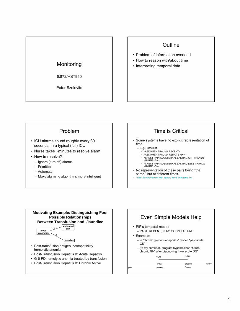
Motivating Example: Distinguishing Four Possible Relationships
Between Transfusion and Jaundice
• Post-transfusion antigen incompatibility hemolytic anemia
• Post-Transfusion Hepatitis B: Acute Hepatitis• G-6-PD hemolytic anemia treated by transfusion• Post-Transfusion Hepatitis B: Chronic Active
bloodtransfusion
abdominalpain
jaundice
?
?
Even Simple Models Help
• PIP’s temporal model:– PAST, RECENT, NOW, SOON, FUTURE
• Example: – in “chronic glomerulonephritis” model, “past acute
GN”– (to my surprise), program hypothesized “future
chronic GN” after diagnosing “now acute GN”
AGN CGN
past present future
past present future
2
What is Time?
• (Macroscopically) unidirectional• Related to causality• May be modeled in various ways
– Continuous quantity, as in differential equations
– Discrete time points, as in discrete event simulations
– Intervals, as in ordinary descriptions of durations, processes, etc.
… or combinations
Continuous View
• Differential equation view of world• States (state variables) evolve according
to their laws
002
0
2
2
xtvgtx
vgtdtdx
gdt
xd
++−=
+−=
−=
Discrete Event View
• Designated (countable) time points• Nothing “interesting” between events• Events may be defined by
– Clock “ticks”– Interactions among objects in universe– Distinguished points in representation of state
variables (e.g., highest point of cannon shell)
What Can Be a Time Point?
• Calendrical point—a specific date/time• Recognizable event—e.g., “when I had my
tonsils out,” or “start of high school,” or “my ninth birthday”
• Now—special, because it moves
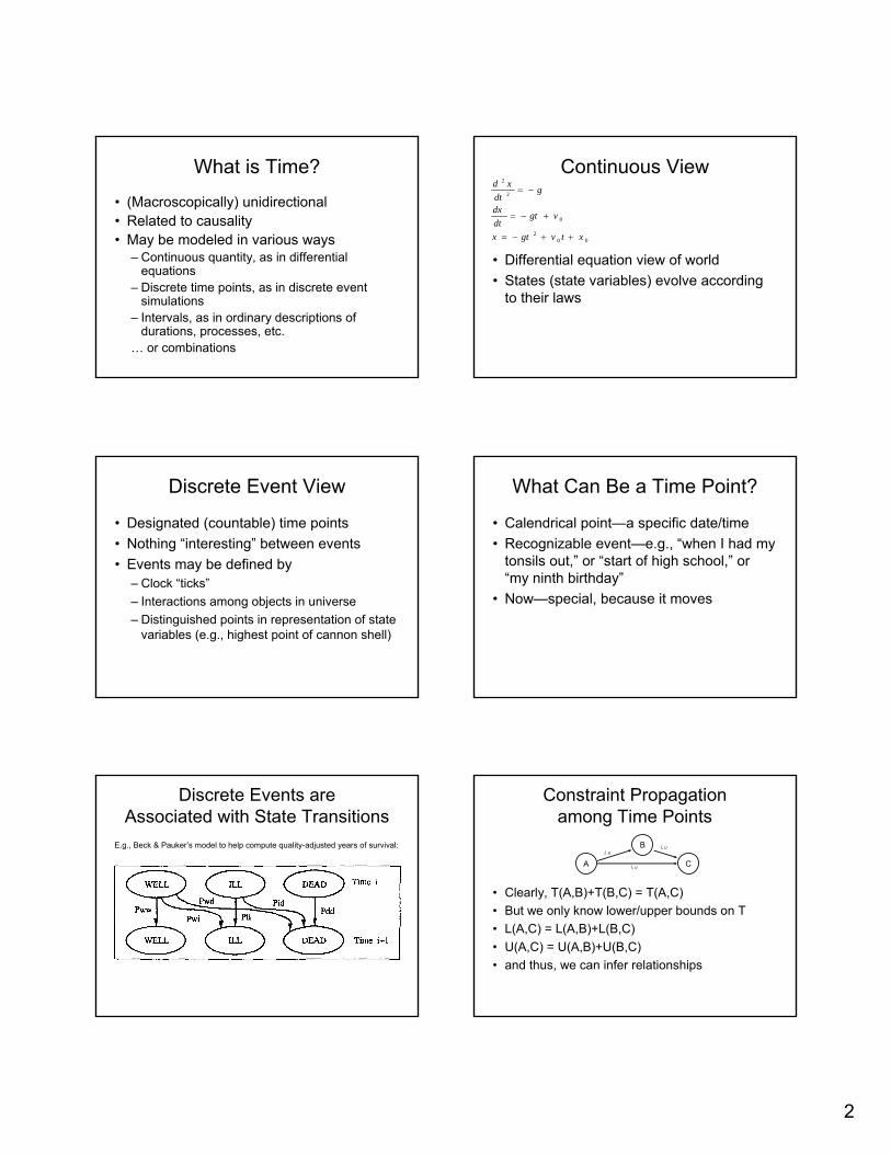
Discrete Events areAssociated with State Transitions
E.g., Beck & Pauker’s model to help compute quality-adjusted years of survival:
Constraint Propagationamong Time Points
• Clearly, T(A,B)+T(B,C) = T(A,C)• But we only know lower/upper bounds on T• L(A,C) = L(A,B)+L(B,C)• U(A,C) = U(A,B)+U(B,C)• and thus, we can infer relationships
A C
Bl, u
l, u
l, u
3
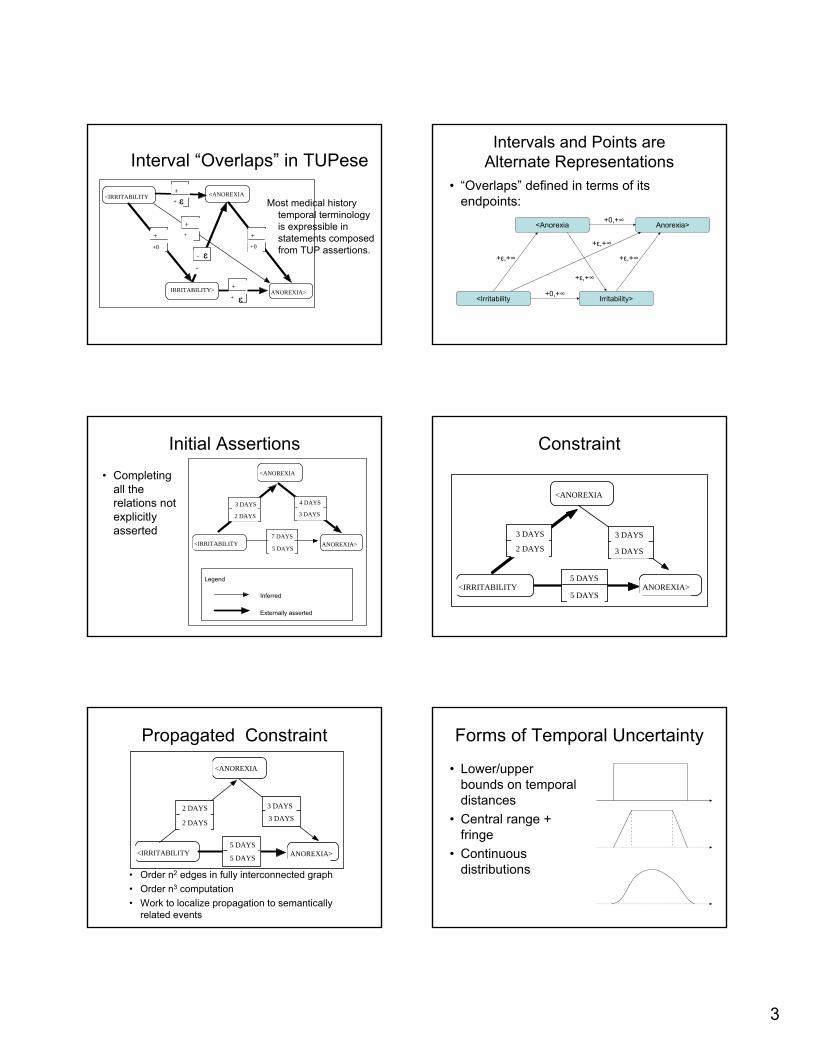
Interval “Overlaps” in TUPese
Most medical history temporal terminology is expressible in statements composed from TUP assertions.
ANOREXIA>
<IRRITABILITY <ANOREXIA
+�+́
+�+0
-�
-́
+�+0
+�+́
+�+́
IRRITABILITY>
ε
ε
ε
Intervals and Points areAlternate Representations
• “Overlaps” defined in terms of its endpoints:
<Irritability Irritability>
<Anorexia Anorexia>+0,+∞
+0,+∞
+ε,+∞ +ε,+∞
+ε,+∞
+ε,+∞
Initial Assertions• Completing
all the relations not explicitly asserted
ANOREXIA>
Externally asserted
<ANOREXIA
<IRRITABILITY
3 DAYS
2 DAYS
7 DAYS
5 DAYS
Legend
Inferred
3 DAYS
4 DAYS
Constraint
<ANOREXIA
<IRRITABILITY ANOREXIA>5 DAYS
5 DAYS
2 DAYS
3 DAYS
3 DAYS
3 DAYS
Propagated Constraint
• Order n2 edges in fully interconnected graph• Order n3 computation• Work to localize propagation to semantically
related events
<ANOREXIA
<IRRITABILITY ANOREXIA>5 DAYS
5 DAYS
3 DAYS2 DAYS
2 DAYS
3 DAYS
Forms of Temporal Uncertainty
• Lower/upper bounds on temporal distances
• Central range + fringe
• Continuous distributions
4
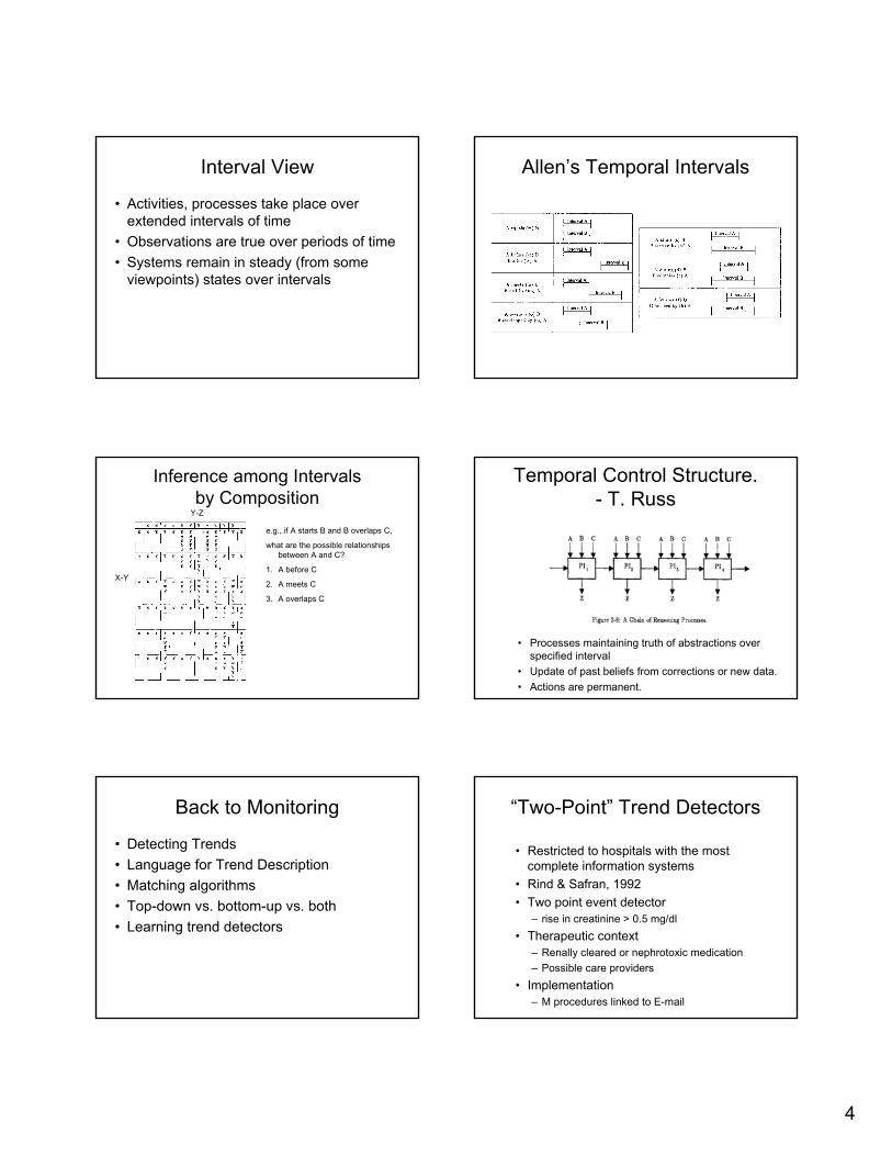
Interval View
• Activities, processes take place over extended intervals of time
• Observations are true over periods of time• Systems remain in steady (from some
viewpoints) states over intervals
Allen’s Temporal Intervals
Inference among Intervalsby Composition
X-Y
Y-Z
e.g., if A starts B and B overlaps C,
what are the possible relationships between A and C?
1. A before C
2. A meets C
3. A overlaps C
Temporal Control Structure. - T. Russ
• Processes maintaining truth of abstractions over specified interval
• Update of past beliefs from corrections or new data.• Actions are permanent.
Back to Monitoring
• Detecting Trends• Language for Trend Description• Matching algorithms• Top-down vs. bottom-up vs. both• Learning trend detectors
“Two-Point” Trend Detectors
• Restricted to hospitals with the most complete information systems
• Rind & Safran, 1992• Two point event detector
– rise in creatinine > 0.5 mg/dl• Therapeutic context
– Renally cleared or nephrotoxic medication– Possible care providers
• Implementation– M procedures linked to E-mail
5
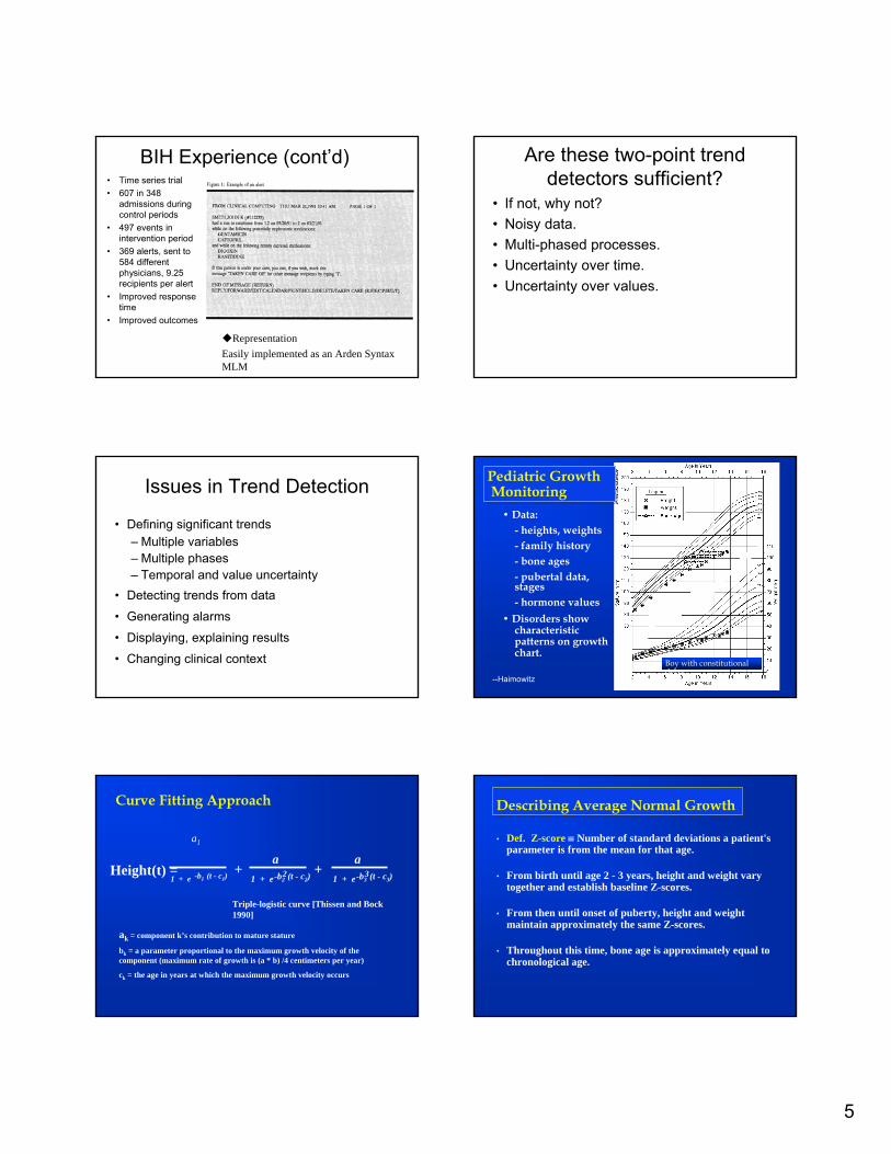
BIH Experience (cont’d)• Time series trial• 607 in 348
admissions during control periods
• 497 events in intervention period
• 369 alerts, sent to 584 different physicians, 9.25 recipients per alert
• Improved response time
• Improved outcomes
RepresentationEasily implemented as an Arden Syntax MLM
Are these two-point trend detectors sufficient?
• If not, why not?• Noisy data.• Multi-phased processes. • Uncertainty over time. • Uncertainty over values.
Issues in Trend Detection
• Defining significant trends– Multiple variables– Multiple phases– Temporal and value uncertainty
• Detecting trends from data
• Generating alarms
• Displaying, explaining results
• Changing clinical context
Pediatric GrowthMonitoring
Pediatric GrowthMonitoring
• Data:- heights, weights - family history - bone ages - pubertal data, stages- hormone values
• Disorders show characteristic patterns on growth chart.
Boy with constitutional delay
--Haimowitz
Curve Fitting Approach
a1
1 + e -b1 (t - c1)
a31 + e-b3 (t - c3)
a21 + e-b2 (t - c2)
+ +Height(t) =
ak = component k’s contribution to mature stature
bk = a parameter proportional to the maximum growth velocity of the component (maximum rate of growth is (a * b) /4 centimeters per year)
ck = the age in years at which the maximum growth velocity occurs
Triple-logistic curve [Thissen and Bock 1990]
Describing Average Normal GrowthDescribing Average Normal Growth
• Def. Z-score ≡ Number of standard deviations a patient's parameter is from the mean for that age.
• From birth until age 2 - 3 years, height and weight vary together and establish baseline Z-scores.
• From then until onset of puberty, height and weight maintain approximately the same Z-scores.
• Throughout this time, bone age is approximately equal to chronological age.
6
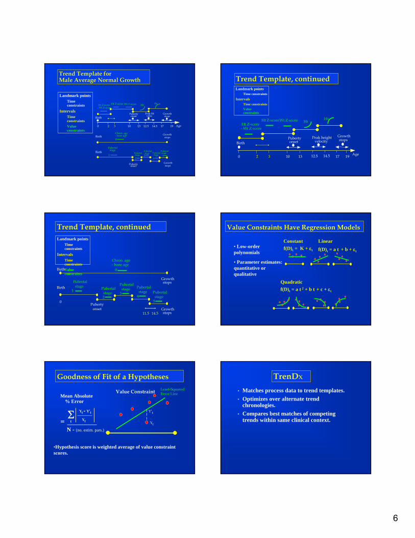
Trend Template for Male Average Normal GrowthTrend Template for Male Average Normal Growth
Landmark pointsTime constraints
IntervalsTime constraintsValue constraints
Age 0 2 3 10 13
Birth
17 19
Ht Z-score - Wt Z-score
Wt Z-score
Pubertyonset
Growthstops
Ht Z-score
BirthGrowth
stopsChron. age- bone age
Pubertyonset
Pubertalstage
Birth Pubertalstage
Growthstops
Ht Ht
12.5 14.5
Peak Htveloc
0
12
3
Pubertalstage Pubertal
stage
4
Pubertalstage5
Trend Template, continuedTrend Template, continued
Age 0
Birth
17 19
Ht Z-score- Wt Z-score
Wt Z-score
10 13
Pubertyonset
Growthstops
Ht Z-score
32
HtHt
12.5 14.5
Peak heightvelocity
Landmark pointsTime constraints
IntervalsTime constraintsValue constraints
Trend Template, continuedTrend Template, continued
Birth
Chron. age- bone age
Pubertyonset
PubertalstageBirth
Pubertalstage
Growthstops
0
Landmark pointsTime constraints
IntervalsTime constraintsValue constraints
1
5
Pubertalstage
4
Pubertalstage
3Pubertalstage2
Growthstops
0
11.5 14.5
Value Constraints Have Regression Models Value Constraints Have Regression Models
Quadraticf(D)t = a t 2 + b t + c + εt
Constantf(D)t = K + εt
Linear
f(D)t = a t + b + εt• Low-order polynomials
• Parameter estimates: quantitative or qualitative
Goodness of Fit of a HypothesesGoodness of Fit of a Hypotheses
Mean Absolute % Error
Least-Squared Error Line
Yt
Y’t
Value Constraint
Σ Yt - Y’t
Ytt=
•Hypothesis score is weighted average of value constraint scores.
N - (no. estim. pars.)
TrenDxTrenDx• Matches process data to trend templates.• Optimizes over alternate trend
chronologies. • Compares best matches of competing
trends within same clinical context.
7
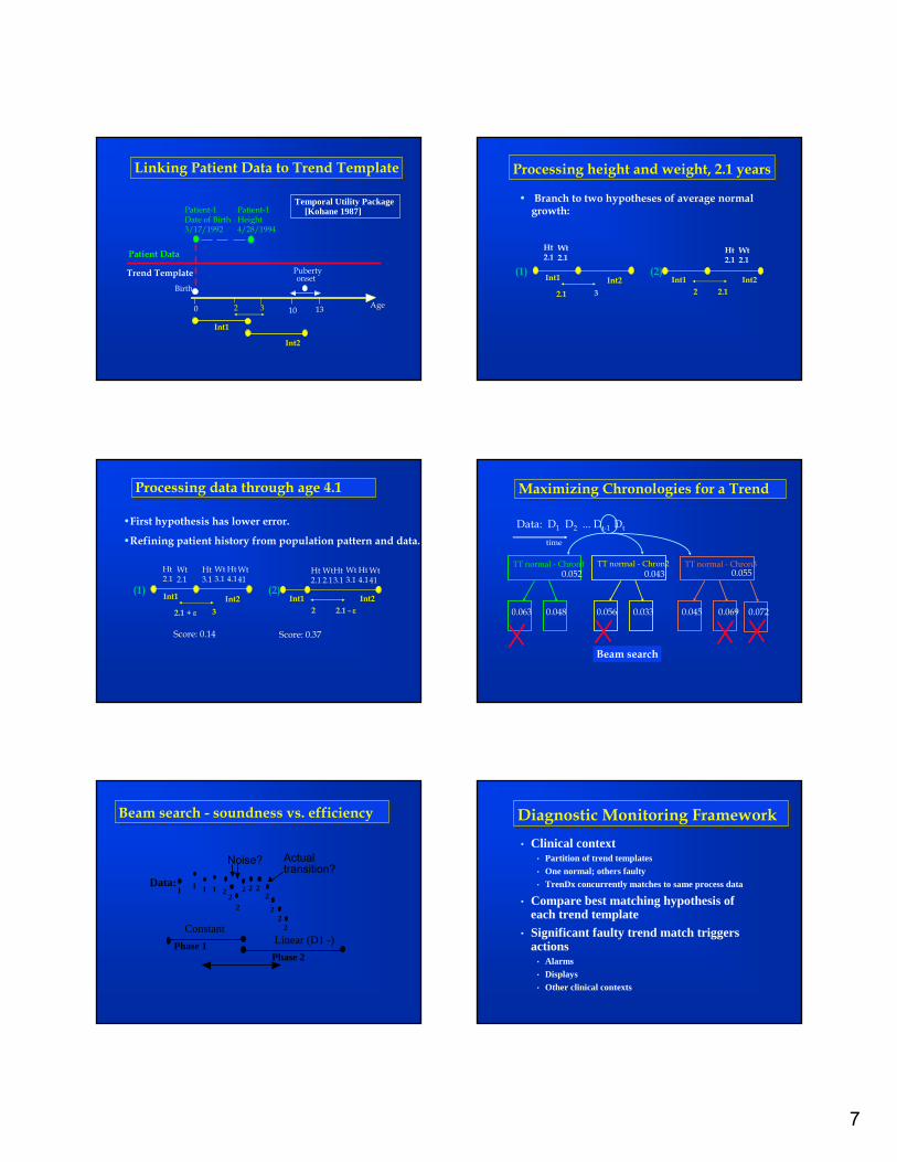
Linking Patient Data to Trend TemplateLinking Patient Data to Trend Template
Age 0
Birth
10 13
Pubertyonset
32
Int1
Int2
Patient-1Date of Birth3/17/1992
Patient Data
Trend Template
Patient-1Height4/28/1994
Temporal Utility Package [Kohane 1987]
Processing height and weight, 2.1 yearsProcessing height and weight, 2.1 years
• Branch to two hypotheses of average normal growth:
Int1 Int22.1 3
Wt2.1
Ht2.1
(1)Int1 Int2
2.12
Ht2.1
Wt2.1
(2)
Processing data through age 4.1 Processing data through age 4.1
Ht3.1
•First hypothesis has lower error.
•Refining patient history from population pattern and data.
Int1 Int22.1 + ε 3
Wt2.1
Ht2.1
(1)Int1 Int2
2.1 - ε2
Ht2.1
Wt2.1
(2)
Score: 0.37Score: 0.14
Wt3.1
Ht4.1
Wt41
Ht3.1
Wt3.1
Ht4.1
Wt41
Maximizing Chronologies for a Trend Maximizing Chronologies for a Trend
Beam search
Data: D1 D2 ... Dt-1 Dt
TT normal - Chron1 TT normal - Chron2 TT normal - Chron3
time
0.052 0.043 0.055
0.0480.063 0.0330.056 0.0720.0690.045
Beam search - soundness vs. efficiencyBeam search - soundness vs. efficiency
Linear (D1 -)Phase 1Phase 2
Data:1 1 1 1
2
22 22
22
2
Noise? Actual transition?
Constant
22
Diagnostic Monitoring FrameworkDiagnostic Monitoring Framework• Clinical context
• Partition of trend templates• One normal; others faulty• TrenDx concurrently matches to same process data
• Compare best matching hypothesis of each trend template
• Significant faulty trend match triggers actions
• Alarms• Displays• Other clinical contexts
8
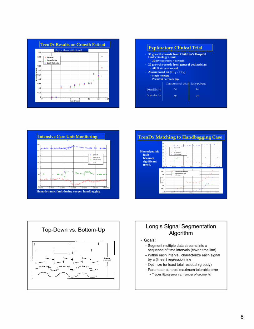
TrenDx Results on Growth Patient TrenDx Results on Growth Patient
B B
B BB B B B B
BB
B
J J
J J
JJ J
JJ J
JJ
H H
H HH H H H H
HH
H
0
0.05
0.1
0.15
0.2
0.25
0.3
0.35
0.4
0.45
0.5
0 2 4 6 8 10 12 14
Scor
e (%
err
or)
Age (years)
B NormalJ Cons DelayH Early Puberty
Patient 39, Const. DelayBoy with constitutional delay
Exploratory Clinical TrialExploratory Clinical Trial• 30 growth records from Children’s Hospital
Endocrinology Clinic• 26 have disorders; 4 normals.
• 20 growth records from general pediatrician • All 20 declared normal
• Alarm based on (TTF - TTN) • Single wide gap• Persistent narrower gap
Constitutional delay Early puberty
Sensitivity
Specificity
.52
.96
.67
.75
Intensive Care Unit MonitoringIntensive Care Unit Monitoring
Hemodynamic fault during oxygen handbagging
BBBB BBBBBBBB BBBB BB BBB B BB BBBBBBB BBBBBBBB
B
BBBBBBBBB
BBBB B B B B B BBB B B B B BBBBBBBB BBBBB BBBB B BBBBBB B
JJJJJ JJJJ JJJJ JJJ JJJ JJJJJ JJJJJ JJJ J J J JJ
JJ
JJJJJJJJJJJJJ J JJ J JJ JJ
JJJJJ JJJJJ JJJ
JJJJJJJJJJJJJJJJJ J
JJJJ
JJJJJJ
JJJJ
JJJJJJJ
JJJJJJ JJJJJJ
HH H HHHH HHHH
HHH
H H HHHHHH HHH HHHHH HHHHHHHHHHHH H HH HHHHHH HHHH H
1
150
70
90
110
130
150
170
190
12:00 AM 12:10 AM 12:20 AM 12:30 AM 12:40 AM 12:50 AM 01:00 AM
B ECG HR
J Mean Art BP
H O2 Saturation
1 FIO2
TrenDx Matching to Handbagging CaseTrenDx Matching to Handbagging Case
Hemodynamicfault becomes significant trend.
J J J J J J J J J J J J J J JJ J J J J J J
1
1
HH
HH H H H H
B B B BB B
B
B B BB B B B B B B B B B B
50
70
90
110
130
150
170
190
12:20 AM 12:22 AM 12:24 AM 12:26 AM 12:28 AM 12:30 AM 12:32 AM
J Mean Art BP
1 FIO2
H O2 Saturation
B ECG Heart Rate
BB B
B B BB
B B
BB B B B B B B B B B
B
B B
B B
B B
B
JJ J
J J JJ
J J
JJ J J J J J J J J J J J
J J J J J J
HH H H H H H H H H H H H H H H HH H H
H
HH
H H
H H
H
0
0.005
0.01
0.015
0.02
0.025
0.03
0.035
0.04
12:20:00 AM 12:22:00 AM 12:24:00 AM 12:26:00 AM 12:28:00 AM 12:30:00 AM 12:32:00 AM
Scor
e (%
Err
or)
Time
B Adequate HandbaggingJ Hemodynamic FaultH Difference
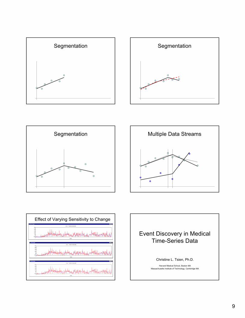
Top-Down vs. Bottom-Up Long’s Signal Segmentation Algorithm
• Goals:– Segment multiple data streams into a
sequence of time intervals (cover time line)– Within each interval, characterize each signal
by a (linear) regression line– Optimize for least total residual (greedy)– Parameter controls maximum tolerable error
• Trades fitting error vs. number of segments
9
Segmentation Segmentation
Segmentation Multiple Data Streams
Effect of Varying Sensitivity to Change
Event Discovery in Medical Time-Series Data
Christine L. Tsien, Ph.D.Harvard Medical School, Boston MA
Massachusetts Institute of Technology, Cambridge MA
10
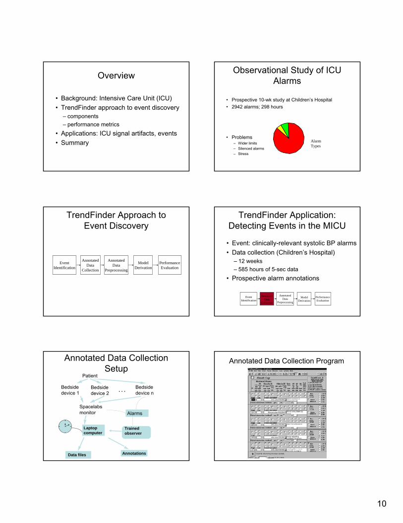
Overview
• Background: Intensive Care Unit (ICU)• TrendFinder approach to event discovery
– components– performance metrics
• Applications: ICU signal artifacts, events• Summary
Observational Study of ICU Alarms
• Prospective 10-wk study at Children’s Hospital• 2942 alarms; 298 hours
• Problems– Wider limits– Silenced alarms– Stress
86%
6%8%
AlarmTypes
TrendFinder Approach to Event Discovery
EventIdentification
AnnotatedData
Collection
AnnotatedData
Preprocessing
ModelDerivation
PerformanceEvaluation
AnnotatedData
Preprocessing
TrendFinder Application: Detecting Events in the MICU
• Event: clinically-relevant systolic BP alarms• Data collection (Children’s Hospital)
– 12 weeks– 585 hours of 5-sec data
• Prospective alarm annotations
AnnotatedData
Collection
EventIdentification
ModelDerivation
PerformanceEvaluation
Annotated Data Collection Setup
Patient
Bedsidedevice 1
Bedsidedevice 2
Bedsidedevice n
Spacelabsmonitor
Laptopcomputer
Data files Annotations
. . .
Alarms
Trainedobserver
Annotated Data Collection Program
11
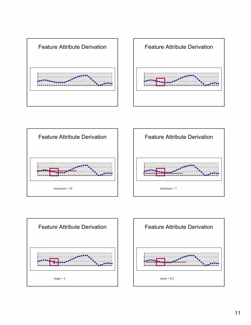
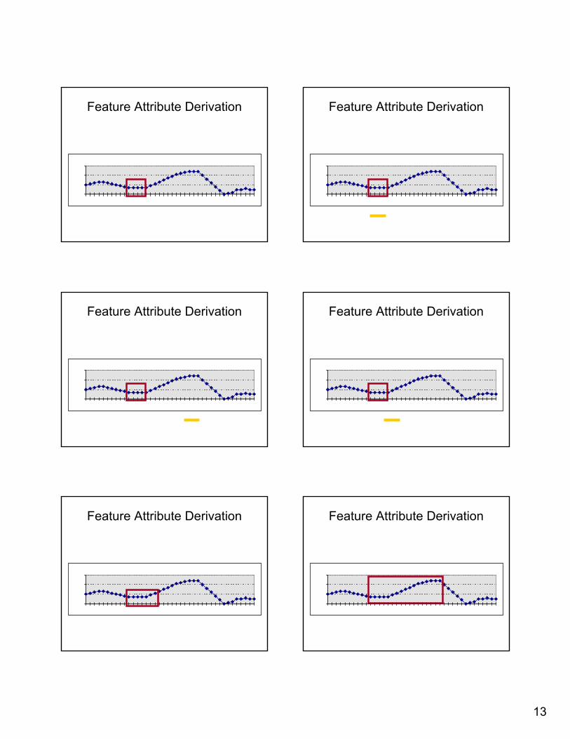
Feature Attribute Derivation Feature Attribute Derivation
Feature Attribute Derivation
maximum = 10
Feature Attribute Derivation
minimum = 7
Feature Attribute Derivation
range = 3
Feature Attribute Derivation
mean = 8.5
12
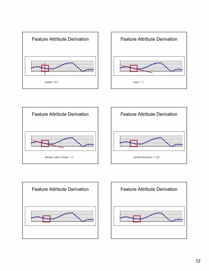
Feature Attribute Derivation
median = 8.5
Feature Attribute Derivation
slope = -1
Feature Attribute Derivation
absolute value of slope = +1
Feature Attribute Derivation
standard deviation = 1.29
Feature Attribute Derivation Feature Attribute Derivation
13
Feature Attribute Derivation Feature Attribute Derivation
Feature Attribute Derivation Feature Attribute Derivation
Feature Attribute Derivation Feature Attribute Derivation
14
Feature Attribute Derivation Feature Attribute Derivation
Feature Attribute Derivation Feature Attribute Derivation
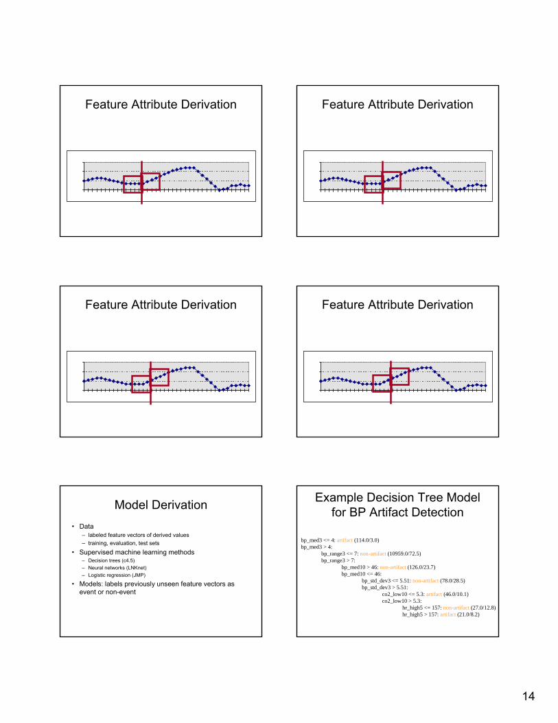
Model Derivation• Data
– labeled feature vectors of derived values– training, evaluation, test sets
• Supervised machine learning methods– Decision trees (c4.5)– Neural networks (LNKnet)– Logistic regression (JMP)
• Models: labels previously unseen feature vectors as event or non-event
Example Decision Tree Model for BP Artifact Detection
bp_med3 <= 4: artifact (114.0/3.0)bp_med3 > 4:
bp_range3 <= 7: non-artifact (10959.0/72.5)bp_range3 > 7:
bp_med10 > 46: non-artifact (126.0/23.7)bp_med10 <= 46:
bp_std_dev3 <= 5.51: non-artifact (78.0/28.5)bp_std_dev3 > 5.51:
co2_low10 <= 5.3: artifact (46.0/10.1)co2_low10 > 5.3:
hr_high5 <= 157: non-artifact (27.0/12.8)hr_high5 > 157: artifact (21.0/8.2)
15
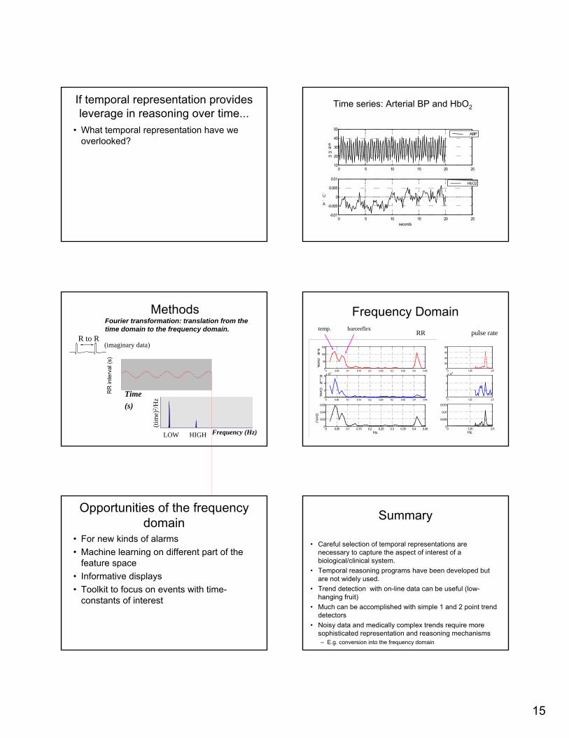
If temporal representation provides leverage in reasoning over time...
• What temporal representation have we overlooked?
0 5 10 15 20 2510
20
30
40
50
mmHg
ABP
0 5 10 15 20 25-0.01
-0.005
0
0.005
0.01
seconds
A.U.
HbO2
Time series: Arterial BP and HbO2
MethodsFourier transformation: translation from the time domain to the frequency domain.
RR
inte
rval
(s)
Time (s)
(imaginary data)
LOW HIGH
(tim
e)2 /H
z
Frequency (Hz)
R to R
0 0.05 0.1 0.15 0.2 0.25 0.3 0.35 0.4 0.450
50
100
150
PSD
BP
0 0.05 0.1 0.15 0.2 0.25 0.3 0.35 0.4 0.450
2
4
6x 10⁻⁵
PSD
NIR
0 0.05 0.1 0.15 0.2 0.25 0.3 0.35 0.4 0.450
0.02
0.04
0.06
Hz.
CSD
Frequency Domainpulse rateRR
baroreflextemp.
0 1.25 2.50
20
40
60
80
0 1.25 2.50
1
2
3x 10⁻⁶
0 1.25 2.50
0.005
0.01
0.015
Hz.
Opportunities of the frequency domain
• For new kinds of alarms• Machine learning on different part of the
feature space• Informative displays• Toolkit to focus on events with time-
constants of interest
Summary
• Careful selection of temporal representations are necessary to capture the aspect of interest of a biological/clinical system.
• Temporal reasoning programs have been developed but are not widely used.
• Trend detection with on-line data can be useful (low-hanging fruit)
• Much can be accomplished with simple 1 and 2 point trend detectors
• Noisy data and medically complex trends require more sophisticated representation and reasoning mechanisms– E.g. conversion into the frequency domain