problem solutions – chapter 2web.eng.fiu.edu/andrian/eel 5543/chapter2.pdf · problem solutions...
TRANSCRIPT
Problem Solutions – Chapter 2
Problem 2.2.1 Solution
(a) We wish to find the value of c that makes the PMF sum up to one.
PN (n) ={
c(1/2)n n = 0, 1, 20 otherwise
(1)
Therefore,∑2
n=0 PN (n) = c + c/2 + c/4 = 1, implying c = 4/7.
(b) The probability that N ≤ 1 is
P [N ≤ 1] = P [N = 0] + P [N = 1] = 4/7 + 2/7 = 6/7 (2)
Problem 2.2.2 SolutionFrom Example 2.5, we can write the PMF of X and the PMF of R as
PX (x) =
⎧⎪⎪⎪⎪⎨⎪⎪⎪⎪⎩
1/8 x = 03/8 x = 13/8 x = 21/8 x = 30 otherwise
PR (r) =
⎧⎨⎩
1/4 r = 03/4 r = 20 otherwise
(1)
From the PMFs PX(x) and PR(r), we can calculate the requested probabilities
(a) P [X = 0] = PX(0) = 1/8.
(b) P [X < 3] = PX(0) + PX(1) + PX(2) = 7/8.
(c) P [R > 1] = PR(2) = 3/4.
Problem 2.2.3 Solution
(a) We must choose c to make the PMF of V sum to one.4∑
v=1
PV (v) = c(12 + 22 + 32 + 42) = 30c = 1 (1)
Hence c = 1/30.
(b) Let U = {u2|u = 1, 2, . . .} so that
P [V ∈ U ] = PV (1) + PV (4) =130
+42
30=
1730
(2)
(c) The probability that V is even is
P [V is even] = PV (2) + PV (4) =22
30+
42
30=
23
(3)
(d) The probability that V > 2 is
P [V > 2] = PV (3) + PV (4) =32
30+
42
30=
56
(4)
35
Problem 2.2.4 Solution
(a) We choose c so that the PMF sums to one.
∑x
PX (x) =c
2+
c
4+
c
8=
7c
8= 1 (1)
Thus c = 8/7.
(b)
P [X = 4] = PX (4) =8
7 · 4 =27
(2)
(c)
P [X < 4] = PX (2) =8
7 · 2 =47
(3)
(d)
P [3 ≤ X ≤ 9] = PX (4) + PX (8) =8
7 · 4 +8
7 · 8 =37
(4)
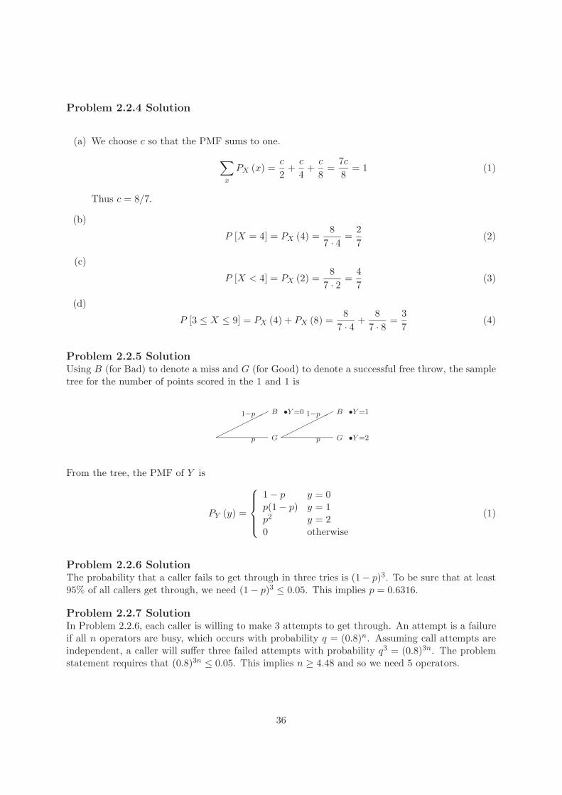
Problem 2.2.5 SolutionUsing B (for Bad) to denote a miss and G (for Good) to denote a successful free throw, the sampletree for the number of points scored in the 1 and 1 is
������ B1−p
Gp������ B1−p
Gp
•Y =0 •Y =1
•Y =2
From the tree, the PMF of Y is
PY (y) =
⎧⎪⎪⎨⎪⎪⎩
1 − p y = 0p(1 − p) y = 1p2 y = 20 otherwise
(1)
Problem 2.2.6 SolutionThe probability that a caller fails to get through in three tries is (1− p)3. To be sure that at least95% of all callers get through, we need (1 − p)3 ≤ 0.05. This implies p = 0.6316.
Problem 2.2.7 SolutionIn Problem 2.2.6, each caller is willing to make 3 attempts to get through. An attempt is a failureif all n operators are busy, which occurs with probability q = (0.8)n. Assuming call attempts areindependent, a caller will suffer three failed attempts with probability q3 = (0.8)3n. The problemstatement requires that (0.8)3n ≤ 0.05. This implies n ≥ 4.48 and so we need 5 operators.
36

Problem 2.2.8 SolutionFrom the problem statement, a single is twice as likely as a double, which is twice as likely as atriple, which is twice as likely as a home-run. If p is the probability of a home run, then
PB (4) = p PB (3) = 2p PB (2) = 4p PB (1) = 8p (1)
Since a hit of any kind occurs with probability of .300, p + 2p + 4p + 8p = 0.300 which impliesp = 0.02. Hence, the PMF of B is
PB (b) =
⎧⎪⎪⎪⎪⎪⎪⎨⎪⎪⎪⎪⎪⎪⎩
0.70 b = 00.16 b = 10.08 b = 20.04 b = 30.02 b = 40 otherwise
(2)
Problem 2.2.9 Solution
(a) In the setup of a mobile call, the phone will send the “SETUP” message up to six times.Each time the setup message is sent, we have a Bernoulli trial with success probability p. Ofcourse, the phone stops trying as soon as there is a success. Using r to denote a successfulresponse, and n a non-response, the sample tree is
����� rp
n1−p����� rp
n1−p����� rp
n1−p����� rp
n1−p����� rp
n1−p����� rp
n1−p
•K=1 •K=2 •K=3 •K=4 •K=5 •K=6
•K=6
(b) We can write the PMF of K, the number of “SETUP” messages sent as
PK (k) =
⎧⎨⎩
(1 − p)k−1p k = 1, 2, . . . , 5(1 − p)5p + (1 − p)6 = (1 − p)5 k = 60 otherwise
(1)
Note that the expression for PK(6) is different because K = 6 if either there was a success ora failure on the sixth attempt. In fact, K = 6 whenever there were failures on the first fiveattempts which is why PK(6) simplifies to (1 − p)5.
(c) Let B denote the event that a busy signal is given after six failed setup attempts. Theprobability of six consecutive failures is P [B] = (1 − p)6.
(d) To be sure that P [B] ≤ 0.02, we need p ≥ 1 − (0.02)1/6 = 0.479.
Problem 2.3.1 Solution
(a) If it is indeed true that Y , the number of yellow M&M’s in a package, is uniformly distributedbetween 5 and 15, then the PMF of Y , is
PY (y) ={
1/11 y = 5, 6, 7, . . . , 150 otherwise
(1)
37

(b)P [Y < 10] = PY (5) + PY (6) + · · · + PY (9) = 5/11 (2)
(c)P [Y > 12] = PY (13) + PY (14) + PY (15) = 3/11 (3)
(d)P [8 ≤ Y ≤ 12] = PY (8) + PY (9) + · · · + PY (12) = 5/11 (4)
Problem 2.3.2 Solution
(a) Each paging attempt is an independent Bernoulli trial with success probability p. The numberof times K that the pager receives a message is the number of successes in n Bernoulli trialsand has the binomial PMF
PK (k) ={ (
nk
)pk(1 − p)n−k k = 0, 1, . . . , n
0 otherwise(1)
(b) Let R denote the event that the paging message was received at least once. The event R hasprobability
P [R] = P [B > 0] = 1 − P [B = 0] = 1 − (1 − p)n (2)
To ensure that P [R] ≥ 0.95 requires that n ≥ ln(0.05)/ ln(1 − p). For p = 0.8, we must haven ≥ 1.86. Thus, n = 2 pages would be necessary.
Problem 2.3.3 SolutionWhether a hook catches a fish is an independent trial with success probability h. The the numberof fish hooked, K, has the binomial PMF
PK (k) ={ (
mk
)hk(1 − h)m−k k = 0, 1, . . . , m
0 otherwise(1)
Problem 2.3.4 Solution
(a) Let X be the number of times the frisbee is thrown until the dog catches it and runs away.Each throw of the frisbee can be viewed as a Bernoulli trial in which a success occurs if thedog catches the frisbee an runs away. Thus, the experiment ends on the first success and Xhas the geometric PMF
PX (x) ={
(1 − p)x−1p x = 1, 2, . . .0 otherwise
(1)
(b) The child will throw the frisbee more than four times iff there are failures on the first 4trials which has probability (1 − p)4. If p = 0.2, the probability of more than four throws is(0.8)4 = 0.4096.
38
Problem 2.3.5 SolutionEach paging attempt is a Bernoulli trial with success probability p where a success occurs if thepager receives the paging message.
(a) The paging message is sent again and again until a success occurs. Hence the number ofpaging messages is N = n if there are n−1 paging failures followed by a paging success. Thatis, N has the geometric PMF
PN (n) ={
(1 − p)n−1p n = 1, 2, . . .0 otherwise
(1)
(b) The probability that no more three paging attempts are required is
P [N ≤ 3] = 1 − P [N > 3] = 1 −∞∑
n=4
PN (n) = 1 − (1 − p)3 (2)
This answer can be obtained without calculation since N > 3 if the first three paging attemptsfail and that event occurs with probability (1 − p)3. Hence, we must choose p to satisfy1 − (1 − p)3 ≥ 0.95 or (1 − p)3 ≤ 0.05. This implies
p ≥ 1 − (0.05)1/3 ≈ 0.6316 (3)
Problem 2.3.6 SolutionThe probability of more than 500,000 bits is
P [B > 500,000] = 1 −500,000∑
b=1
PB (b) (1)
= 1 − p
500,000∑b=1
(1 − p)b−1 (2)
Math Fact B.4 implies that (1−x)∑500,000
b=1 xb−1 = 1−x500,000. Substituting, x = 1− p, we obtain:
P [B > 500,000] = 1 − (1 − (1 − p)500,000) (3)
= (1 − 0.25 × 10⁻⁵)500,000 ≈ exp(−500,000/400,000) = 0.29. (4)
Problem 2.3.7 SolutionSince an average of T/5 buses arrive in an interval of T minutes, buses arrive at the bus stop at arate of 1/5 buses per minute.
(a) From the definition of the Poisson PMF, the PMF of B, the number of buses in T minutes,is
PB (b) ={
(T/5)be−T/5/b! b = 0, 1, . . .0 otherwise
(1)
(b) Choosing T = 2 minutes, the probability that three buses arrive in a two minute interval is
PB (3) = (2/5)3e−2/5/3! ≈ 0.0072 (2)
39

(c) By choosing T = 10 minutes, the probability of zero buses arriving in a ten minute interval is
PB (0) = e−10/5/0! = e−2 ≈ 0.135 (3)
(d) The probability that at least one bus arrives in T minutes is
P [B ≥ 1] = 1 − P [B = 0] = 1 − e−T/5 ≥ 0.99 (4)
Rearranging yields T ≥ 5 ln 100 ≈ 23.0 minutes.
Problem 2.3.8 Solution
(a) If each message is transmitted 8 times and the probability of a successful transmission is p,then the PMF of N , the number of successful transmissions has the binomial PMF
PN (n) ={ (
8n
)pn(1 − p)8−n n = 0, 1, . . . , 8
0 otherwise(1)
(b) The indicator random variable I equals zero if and only if N = 8. Hence,
P [I = 0] = P [N = 0] = 1 − P [I = 1] (2)
Thus, the complete expression for the PMF of I is
PI (i) =
⎧⎨⎩
(1 − p)8 i = 01 − (1 − p)8 i = 10 otherwise
(3)
Problem 2.3.9 SolutionThe requirement that
∑nx=1 PX(x) = 1 implies
n = 1 : c(1)[11
]= 1 c(1) = 1 (1)
n = 2 : c(2)[11
+12
]= 1 c(2) =
23
(2)
n = 3 : c(3)[11
+12
+13
]= 1 c(3) =
611
(3)
n = 4 : c(4)[11
+12
+13
+14
]= 1 c(4) =
1225
(4)
n = 5 : c(5)[11
+12
+13
+14
+15
]= 1 c(5) =
1225
(5)
n = 6 : c(6)[11
+12
+13
+14
+16
]= 1 c(6) =
2049
(6)
As an aside, find c(n) for large values of n is easy using the recursion
1c(n + 1)
=1
c(n)+
1n + 1
. (7)
40

Problem 2.3.10 Solution
(a) We can view whether each caller knows the birthdate as a Bernoulli trial. As a result, L isthe number of trials needed for 6 successes. That is, L has a Pascal PMF with parametersp = 0.75 and k = 6 as defined by Definition 2.8. In particular,
PL (l) ={ (
l−15
)(0.75)6(0.25)l−6 l = 6, 7, . . .
0 otherwise(1)
(b) The probability of finding the winner on the tenth call is
PL (10) =(
95
)(0.75)6(0.25)4 ≈ 0.0876 (2)
(c) The probability that the station will need nine or more calls to find a winner is
P [L ≥ 9] = 1 − P [L < 9] (3)= 1 − PL (6) − PL (7) − PL (8) (4)
= 1 − (0.75)6[1 + 6(0.25) + 21(0.25)2] ≈ 0.321 (5)
Problem 2.3.11 SolutionThe packets are delay sensitive and can only be retransmitted d times. For t < d, a packet istransmitted t times if the first t− 1 attempts fail followed by a successful transmission on attemptt. Further, the packet is transmitted d times if there are failures on the first d − 1 transmissions,no matter what the outcome of attempt d. So the random variable T , the number of times that apacket is transmitted, can be represented by the following PMF.
PT (t) =
⎧⎨⎩
p(1 − p)t−1 t = 1, 2, . . . , d − 1(1 − p)d−1 t = d0 otherwise
(1)
Problem 2.3.12 Solution
(a) Since each day is independent of any other day, P [W33] is just the probability that a winninglottery ticket was bought. Similarly for P [L87] and P [N99] become just the probability that alosing ticket was bought and that no ticket was bought on a single day, respectively. Therefore
P [W33] = p/2 P [L87] = (1 − p)/2 P [N99] = 1/2 (1)
(b) Suppose we say a success occurs on the kth trial if on day k we buy a ticket. Otherwise, afailure occurs. The probability of success is simply 1/2. The random variable K is just thenumber of trials until the first success and has the geometric PMF
PK (k) ={
(1/2)(1/2)k−1 = (1/2)k k = 1, 2, . . .0 otherwise
(2)
41

(c) The probability that you decide to buy a ticket and it is a losing ticket is (1−p)/2, independentof any other day. If we view buying a losing ticket as a Bernoulli success, R, the number oflosing lottery tickets bought in m days, has the binomial PMF
PR (r) ={ (
mr
)[(1 − p)/2]r[(1 + p)/2]m−r r = 0, 1, . . . , m
0 otherwise(3)
(d) Letting D be the day on which the j-th losing ticket is bought, we can find the probabilitythat D = d by noting that j−1 losing tickets must have been purchased in the d−1 previousdays. Therefore D has the Pascal PMF
PD (d) =
{ (d−1j−1
)[(1 − p)/2]j [(1 + p)/2]d−j d = j, j + 1, . . .
0 otherwise(4)
Problem 2.3.13 Solution
(a) Let Sn denote the event that the Sixers win the series in n games. Similarly, Cn is the eventthat the Celtics in in n games. The Sixers win the series in 3 games if they win three straight,which occurs with probability
P [S3] = (1/2)3 = 1/8 (1)
The Sixers win the series in 4 games if they win two out of the first three games and theywin the fourth game so that
P [S4] =(
32
)(1/2)3(1/2) = 3/16 (2)
The Sixers win the series in five games if they win two out of the first four games and thenwin game five. Hence,
P [S5] =(
42
)(1/2)4(1/2) = 3/16 (3)
By symmetry, P [Cn] = P [Sn]. Further we observe that the series last n games if either theSixers or the Celtics win the series in n games. Thus,
P [N = n] = P [Sn] + P [Cn] = 2P [Sn] (4)
Consequently, the total number of games, N , played in a best of 5 series between the Celticsand the Sixers can be described by the PMF
PN (n) =
⎧⎪⎪⎨⎪⎪⎩
2(1/2)3 = 1/4 n = 32(31
)(1/2)4 = 3/8 n = 4
2(42
)(1/2)5 = 3/8 n = 5
0 otherwise
(5)
(b) For the total number of Celtic wins W , we note that if the Celtics get w < 3 wins, then theSixers won the series in 3 + w games. Also, the Celtics win 3 games if they win the series in3,4, or 5 games. Mathematically,
P [W = w] ={
P [S3+w] w = 0, 1, 2P [C3] + P [C4] + P [C5] w = 3
(6)
42
Thus, the number of wins by the Celtics, W , has the PMF shown below.
PW (w) =
⎧⎪⎪⎪⎪⎨⎪⎪⎪⎪⎩
P [S3] = 1/8 w = 0P [S4] = 3/16 w = 1P [S5] = 3/16 w = 21/8 + 3/16 + 3/16 = 1/2 w = 30 otherwise
(7)
(c) The number of Celtic losses L equals the number of Sixers’ wins WS . This implies PL(l) =PWS
(l). Since either team is equally likely to win any game, by symmetry, PWS(w) = PW (w).
This implies PL(l) = PWS(l) = PW (l). The complete expression of for the PMF of L is
PL (l) = PW (l) =
⎧⎪⎪⎪⎪⎨⎪⎪⎪⎪⎩
1/8 l = 03/16 l = 13/16 l = 21/2 l = 30 otherwise
(8)
Problem 2.3.14 SolutionSince a and b are positive, let K be a binomial random variable for n trials and success probabilityp = a/(a + b). First, we observe that the sum of over all possible values of the PMF of K is
n∑k=0
PK (k) =n∑
k=0
(n
k
)pk(1 − p)n−k (1)
=n∑
k=0
(n
k
)(a
a + b
)k ( b
a + b
)n−k
(2)
=∑n
k=0
(nk
)akbn−k
(a + b)n(3)
Since∑n
k=0 PK(k) = 1, we see that
(a + b)n = (a + b)nn∑
k=0
PK (k) =n∑
k=0
(n
k
)akbn−k (4)
Problem 2.4.1 SolutionUsing the CDF given in the problem statement we find that
(a) P [Y < 1] = 0
(b) P [Y ≤ 1] = 1/4
(c) P [Y > 2] = 1 − P [Y ≤ 2] = 1 − 1/2 = 1/2
(d) P [Y ≥ 2] = 1 − P [Y < 2] = 1 − 1/4 = 3/4
(e) P [Y = 1] = 1/4
43

(f) P [Y = 3] = 1/2
(g) From the staircase CDF of Problem 2.4.1, we see that Y is a discrete random variable. Thejumps in the CDF occur at at the values that Y can take on. The height of each jump equalsthe probability of that value. The PMF of Y is
PY (y) =
⎧⎪⎪⎨⎪⎪⎩
1/4 y = 11/4 y = 21/2 y = 30 otherwise
(1)
Problem 2.4.2 Solution
(a) The given CDF is shown in the diagram below.
−2 −1 0 1 2
00.20.40.60.8
1
x
FX(x
)
FX (x) =
⎧⎪⎪⎨⎪⎪⎩
0 x < −10.2 −1 ≤ x < 00.7 0 ≤ x < 11 x ≥ 1
(1)
(b) The corresponding PMF of X is
PX (x) =
⎧⎪⎪⎨⎪⎪⎩
0.2 x = −10.5 x = 00.3 x = 10 otherwise
(2)
Problem 2.4.3 Solution
(a) Similar to the previous problem, the graph of the CDF is shown below.
−3 0 5 7
00.20.40.60.8
1
x
FX(x
)
FX (x) =
⎧⎪⎪⎨⎪⎪⎩
0 x < −30.4 −3 ≤ x < 50.8 5 ≤ x < 71 x ≥ 7
(1)
(b) The corresponding PMF of X is
PX (x) =
⎧⎪⎪⎨⎪⎪⎩
0.4 x = −30.4 x = 50.2 x = 70 otherwise
(2)
44

Problem 2.4.4 SolutionLet q = 1 − p, so the PMF of the geometric (p) random variable K is
PK (k) ={
pqk−1 k = 1, 2, . . . ,0 otherwise.
(1)
For any integer k ≥ 1, the CDF obeys
FK (k) =k∑
j=1
PK (j) =k∑
j=1
pqj−1 = 1 − qk. (2)
Since K is integer valued, FK(k) = FK(�k�) for all integer and non-integer values of k. (If thispoint is not clear, you should review Example 2.24.) Thus, the complete expression for the CDFof K is
FK (k) ={
0 k < 1,
1 − (1 − p)�k� k ≥ 1.(3)
Problem 2.4.5 SolutionSince mushrooms occur with probability 2/3, the number of pizzas sold before the first mushroompizza is N = n < 100 if the first n pizzas do not have mushrooms followed by mushrooms on pizzan + 1. Also, it is possible that N = 100 if all 100 pizzas are sold without mushrooms. the resultingPMF is
PN (n) =
⎧⎨⎩
(1/3)n(2/3) n = 0, 1, . . . , 99(1/3)100 n = 1000 otherwise
(1)
For integers n < 100, the CDF of N obeys
FN (n) =n∑
i=0
PN (i) =n∑
i=0
(1/3)i(2/3) = 1 − (1/3)n+1 (2)
A complete expression for FN (n) must give a valid answer for every value of n, including non-integervalues. We can write the CDF using the floor function �x� which denote the largest integer lessthan or equal to X. The complete expression for the CDF is
FN (x) =
⎧⎨⎩
0 x < 01 − (1/3)�x�+1 0 ≤ x < 1001 x ≥ 100
(3)
Problem 2.4.6 SolutionFrom Problem 2.2.8, the PMF of B is
PB (b) =
⎧⎪⎪⎪⎪⎪⎪⎨⎪⎪⎪⎪⎪⎪⎩
0.70 b = 00.16 b = 10.08 b = 20.04 b = 30.02 b = 40 otherwise
(1)
45

The corresponding CDF is
−1 0 1 2 3 4 50
0.250.5
0.751
b
FB(b
)
FB (b) =
⎧⎪⎪⎪⎪⎪⎪⎨⎪⎪⎪⎪⎪⎪⎩
0 b < 00.70 0 ≤ b < 10.86 1 ≤ b < 20.94 2 ≤ b < 30.98 3 ≤ b < 41.0 b ≥ 4
(2)
Problem 2.4.7 SolutionIn Problem 2.2.5, we found the PMF of Y . This PMF, and its corresponding CDF are
PY (y) =
⎧⎪⎪⎨⎪⎪⎩
1 − p y = 0p(1 − p) y = 1p2 y = 20 otherwise
FY (y) =
⎧⎪⎪⎨⎪⎪⎩
0 y < 01 − p 0 ≤ y < 11 − p2 1 ≤ y < 21 y ≥ 2
(1)
For the three values of p, the CDF resembles
−1 0 1 2 3
00.250.5
0.751
y
FY(y
)
−1 0 1 2 3
00.250.5
0.751
y
FY(y
)
−1 0 1 2 3
00.250.5
0.751
y
FY(y
)
p = 1/4 p = 1/2 p = 3/4
(2)
Problem 2.4.8 SolutionFrom Problem 2.2.9, the PMF of the number of call attempts is
PN (n) =
⎧⎨⎩
(1 − p)k−1p k = 1, 2, . . . , 5(1 − p)5p + (1 − p)6 = (1 − p)5 k = 60 otherwise
(1)
For p = 1/2, the PMF can be simplified to
PN (n) =
⎧⎨⎩
(1/2)n n = 1, 2, . . . , 5(1/2)5 n = 60 otherwise
(2)
The corresponding CDF of N is
0 1 2 3 4 5 6 7
00.250.5
0.751
n
FN(n
)
FN (n) =
⎧⎪⎪⎪⎪⎪⎪⎪⎪⎨⎪⎪⎪⎪⎪⎪⎪⎪⎩
0 n < 11/2 1 ≤ n < 23/4 2 ≤ n < 37/8 3 ≤ n < 415/16 4 ≤ n < 531/32 5 ≤ n < 61 n ≥ 6
(3)
46

Problem 2.5.1 SolutionFor this problem, we just need to pay careful attention to the definitions of mode and median.
(a) The mode must satisfy PX(xmod) ≥ PX(x) for all x. In the case of the uniform PMF, anyinteger x′ between 1 and 100 is a mode of the random variable X. Hence, the set of all modesis
Xmod = {1, 2, . . . , 100} (1)
(b) The median must satisfy P [X < xmed] = P [X > xmed]. Since
P [X ≤ 50] = P [X ≥ 51] = 1/2 (2)
we observe that xmed = 50.5 is a median since it satisfies
P [X < xmed] = P [X > xmed] = 1/2 (3)
In fact, for any x′ satisfying 50 < x′ < 51, P [X < x′] = P [X > x′] = 1/2. Thus,
Xmed = {x|50 < x < 51} (4)
Problem 2.5.2 SolutionVoice calls and data calls each cost 20 cents and 30 cents respectively. Furthermore the respectiveprobabilities of each type of call are 0.6 and 0.4.
(a) Since each call is either a voice or data call, the cost of one call can only take the two valuesassociated with the cost of each type of call. Therefore the PMF of X is
PX (x) =
⎧⎨⎩
0.6 x = 200.4 x = 300 otherwise
(1)
(b) The expected cost, E[C], is simply the sum of the cost of each type of call multiplied by theprobability of such a call occurring.
E [C] = 20(0.6) + 30(0.4) = 24 cents (2)
Problem 2.5.3 SolutionFrom the solution to Problem 2.4.1, the PMF of Y is
PY (y) =
⎧⎪⎪⎨⎪⎪⎩
1/4 y = 11/4 y = 21/2 y = 30 otherwise
(1)
The expected value of Y is
E [Y ] =∑
y
yPY (y) = 1(1/4) + 2(1/4) + 3(1/2) = 9/4 (2)
47
Problem 2.5.4 SolutionFrom the solution to Problem 2.4.2, the PMF of X is
PX (x) =
⎧⎪⎪⎨⎪⎪⎩
0.2 x = −10.5 x = 00.3 x = 10 otherwise
(1)
The expected value of X is
E [X] =∑
x
xPX (x) = −1(0.2) + 0(0.5) + 1(0.3) = 0.1 (2)
Problem 2.5.5 SolutionFrom the solution to Problem 2.4.3, the PMF of X is
PX (x) =
⎧⎪⎪⎨⎪⎪⎩
0.4 x = −30.4 x = 50.2 x = 70 otherwise
(1)
The expected value of X is
E [X] =∑
x
xPX (x) = −3(0.4) + 5(0.4) + 7(0.2) = 2.2 (2)
Problem 2.5.6 SolutionFrom Definition 2.7, random variable X has PMF
PX (x) ={ (
4x
)(1/2)4 x = 0, 1, 2, 3, 4
0 otherwise(1)
The expected value of X is
E [X] =4∑
x=0
xPX (x) = 0(
40
)124
+ 1(
41
)124
+ 2(
42
)124
+ 3(
43
)124
+ 4(
44
)124
(2)
= [4 + 12 + 12 + 4]/24 = 2 (3)
Problem 2.5.7 SolutionFrom Definition 2.7, random variable X has PMF
PX (x) ={ (
5x
)(1/2)5 x = 0, 1, 2, 3, 4, 5
0 otherwise(1)
The expected value of X is
E [X] =5∑
x=0
xPX (x) (2)
= 0(
50
)125
+ 1(
51
)125
+ 2(
52
)125
+ 3(
53
)125
+ 4(
54
)125
+ 5(
55
)125
(3)
= [5 + 20 + 30 + 20 + 5]/25 = 2.5 (4)
48
Problem 2.5.8 SolutionThe following experiments are based on a common model of packet transmissions in data networks.In these networks, each data packet contains a cylic redundancy check (CRC) code that permitsthe receiver to determine whether the packet was decoded correctly. In the following, we assumethat a packet is corrupted with probability ε = 0.001, independent of whether any other packet iscorrupted.
(a) Let X = 1 if a data packet is decoded correctly; otherwise X = 0. Random variable X is aBernoulli random variable with PMF
PX (x) =
⎧⎨⎩
0.001 x = 00.999 x = 10 otherwise
(1)
The parameter ε = 0.001 is the probability a packet is corrupted. The expected value of X is
E [X] = 1 − ε = 0.999 (2)
(b) Let Y denote the number of packets received in error out of 100 packets transmitted. Y hasthe binomial PMF
PY (y) ={ (
100y
)(0.001)y(0.999)100−y y = 0, 1, . . . , 100
0 otherwise(3)
The expected value of Y isE [Y ] = 100ε = 0.1 (4)
(c) Let L equal the number of packets that must be received to decode 5 packets in error. L hasthe Pascal PMF
PL (l) ={ (
l−14
)(0.001)5(0.999)l−5 l = 5, 6, . . .
0 otherwise(5)
The expected value of L is
E [L] =5ε
=5
0.001= 5000 (6)
(d) If packet arrivals obey a Poisson model with an average arrival rate of 1000 packets persecond, then the number N of packets that arrive in 5 seconds has the Poisson PMF
PN (n) ={
5000ne−5000/n! n = 0, 1, . . .0 otherwise
(7)
The expected value of N is E[N ] = 5000.
Problem 2.5.9 SolutionIn this ”double-or-nothing” type game, there are only two possible payoffs. The first is zero dollars,which happens when we lose 6 straight bets, and the second payoff is 64 dollars which happensunless we lose 6 straight bets. So the PMF of Y is
PY (y) =
⎧⎨⎩
(1/2)6 = 1/64 y = 01 − (1/2)6 = 63/64 y = 640 otherwise
(1)
The expected amount you take home is
E [Y ] = 0(1/64) + 64(63/64) = 63 (2)
So, on the average, we can expect to break even, which is not a very exciting proposition.
49
Problem 2.5.10 SolutionBy the definition of the expected value,
E [Xn] =n∑
x=1
x
(n
x
)px(1 − p)n−x (1)
= np
n∑x=1
(n − 1)!(x − 1)!(n − 1 − (x − 1))!
px−1(1 − p)n−1−(x−1) (2)
With the substitution x′ = x − 1, we have
E [Xn] = np
n−1∑x′=0
(n − 1
x′
)px′
(1 − p)n−x′
︸ ︷︷ ︸1
= np
n−1∑x′=0
PXn−1 (x) = np (3)
The above sum is 1 because it is the sum of a binomial random variable for n − 1 trials over allpossible values.
Problem 2.5.11 SolutionWe write the sum as a double sum in the following way:
∞∑i=0
P [X > i] =∞∑i=0
∞∑j=i+1
PX (j) (1)
At this point, the key step is to reverse the order of summation. You may need to make a sketchof the feasible values for i and j to see how this reversal occurs. In this case,
∞∑i=0
P [X > i] =∞∑
j=1
j−1∑i=0
PX (j) =∞∑
j=1
jPX (j) = E [X] (2)
Problem 2.6.1 SolutionFrom the solution to Problem 2.4.1, the PMF of Y is
PY (y) =
⎧⎪⎪⎨⎪⎪⎩
1/4 y = 11/4 y = 21/2 y = 30 otherwise
(1)
(a) Since Y has range SY = {1, 2, 3}, the range of U = Y 2 is SU = {1, 4, 9}. The PMF of U canbe found by observing that
P [U = u] = P[Y 2 = u
]= P
[Y =
√u]+ P
[Y = −√
u]
(2)
Since Y is never negative, PU (u) = PY (√
u). Hence,
PU (1) = PY (1) = 1/4 PU (4) = PY (2) = 1/4 PU (9) = PY (3) = 1/2 (3)
For all other values of u, PU (u) = 0. The complete expression for the PMF of U is
PU (u) =
⎧⎪⎪⎨⎪⎪⎩
1/4 u = 11/4 u = 41/2 u = 90 otherwise
(4)
50
(b) From the PMF, it is straighforward to write down the CDF.
FU (u) =
⎧⎪⎪⎨⎪⎪⎩
0 u < 11/4 1 ≤ u < 41/2 4 ≤ u < 91 u ≥ 9
(5)
(c) From Definition 2.14, the expected value of U is
E [U ] =∑
u
uPU (u) = 1(1/4) + 4(1/4) + 9(1/2) = 5.75 (6)
From Theorem 2.10, we can calculate the expected value of U as
E [U ] = E[Y 2]
=∑
y
y2PY (y) = 12(1/4) + 22(1/4) + 32(1/2) = 5.75 (7)
As we expect, both methods yield the same answer.
Problem 2.6.2 SolutionFrom the solution to Problem 2.4.2, the PMF of X is
PX (x) =
⎧⎪⎪⎨⎪⎪⎩
0.2 x = −10.5 x = 00.3 x = 10 otherwise
(1)
(a) The PMF of V = |X| satisfies
PV (v) = P [|X| = v] = PX (v) + PX (−v) (2)
In particular,
PV (0) = PX (0) = 0.5 PV (1) = PX (−1) + PX (1) = 0.5 (3)
The complete expression for the PMF of V is
PV (v) =
⎧⎨⎩
0.5 v = 00.5 v = 10 otherwise
(4)
(b) From the PMF, we can construct the staircase CDF of V .
FV (v) =
⎧⎨⎩
0 v < 00.5 0 ≤ v < 11 v ≥ 1
(5)
(c) From the PMF PV (v), the expected value of V is
E [V ] =∑
v
PV (v) = 0(1/2) + 1(1/2) = 1/2 (6)
You can also compute E[V ] directly by using Theorem 2.10.
51

Problem 2.6.3 SolutionFrom the solution to Problem 2.4.3, the PMF of X is
PX (x) =
⎧⎪⎪⎨⎪⎪⎩
0.4 x = −30.4 x = 50.2 x = 70 otherwise
(1)
(a) The PMF of W = −X satisfies
PW (w) = P [−X = w] = PX (−w) (2)
This implies
PW (−7) = PX (7) = 0.2 PW (−5) = PX (5) = 0.4 PW (3) = PX (−3) = 0.4 (3)
The complete PMF for W is
PW (w) =
⎧⎪⎪⎨⎪⎪⎩
0.2 w = −70.4 w = −50.4 w = 30 otherwise
(4)
(b) From the PMF, the CDF of W is
FW (w) =
⎧⎪⎪⎨⎪⎪⎩
0 w < −70.2 −7 ≤ w < −50.6 −5 ≤ w < 31 w ≥ 3
(5)
(c) From the PMF, W has expected value
E [W ] =∑w
wPW (w) = −7(0.2) + −5(0.4) + 3(0.4) = −2.2 (6)
Problem 2.6.4 SolutionA tree for the experiment is
������� D=99.751/3
D=1001/3
������� D=100.251/3
•C=100074.75
•C=10100
•C=10125.13
Thus C has three equally likely outcomes. The PMF of C is
PC (c) ={
1/3 c = 100,074.75, 10,100, 10,125.130 otherwise
(1)
52
Problem 2.6.5 Solution
(a) The source continues to transmit packets until one is received correctly. Hence, the totalnumber of times that a packet is transmitted is X = x if the first x− 1 transmissions were inerror. Therefore the PMF of X is
PX (x) ={
qx−1(1 − q) x = 1, 2, . . .0 otherwise
(1)
(b) The time required to send a packet is a millisecond and the time required to send an acknowl-edgment back to the source takes another millisecond. Thus, if X transmissions of a packetare needed to send the packet correctly, then the packet is correctly received after T = 2X−1milliseconds. Therefore, for an odd integer t > 0, T = t iff X = (t + 1)/2. Thus,
PT (t) = PX ((t + 1)/2) ={
q(t−1)/2(1 − q) t = 1, 3, 5, . . .0 otherwise
(2)
Problem 2.6.6 SolutionThe cellular calling plan charges a flat rate of $20 per month up to and including the 30th minute,and an additional 50 cents for each minute over 30 minutes. Knowing that the time you spend onthe phone is a geometric random variable M with mean 1/p = 30, the PMF of M is
PM (m) ={
(1 − p)m−1p m = 1, 2, . . .0 otherwise
(1)
The monthly cost, C obeys
PC (20) = P [M ≤ 30] =30∑
m=1
(1 − p)m−1p = 1 − (1 − p)30 (2)
When M ≥ 30, C = 20 + (M − 30)/2 or M = 2C − 10. Thus,
PC (c) = PM (2c − 10) c = 20.5, 21, 21.5, . . . (3)
The complete PMF of C is
PC (c) ={
1 − (1 − p)30 c = 20(1 − p)2c−10−1p c = 20.5, 21, 21.5, . . .
(4)
Problem 2.7.1 SolutionFrom the solution to Quiz 2.6, we found that T = 120 − 15N . By Theorem 2.10,
E [T ] =∑
n∈SN
(120 − 15n)PN (n) (1)
= 0.1(120) + 0.3(120 − 15) + 0.3(120 − 30) + 0.3(120 − 45) = 93 (2)
Also from the solution to Quiz 2.6, we found that
PT (t) =
⎧⎨⎩
0.3 t = 75, 90, 1050.1 t = 1200 otherwise
(3)
53
Using Definition 2.14,
E [T ] =∑t∈ST
tPT (t) = 0.3(75) + 0.3(90) + 0.3(105) + 0.1(120) = 93 (4)
As expected, the two calculations give the same answer.
Problem 2.7.2 SolutionWhether a lottery ticket is a winner is a Bernoulli trial with a success probability of 0.001. If webuy one every day for 50 years for a total of 50 · 365 = 18250 tickets, then the number of winningtickets T is a binomial random variable with mean
E [T ] = 18250(0.001) = 18.25 (1)
Since each winning ticket grosses $1000, the revenue we collect over 50 years is R = 1000T dollars.The expected revenue is
E [R] = 1000E [T ] = 18250 (2)
But buying a lottery ticket everyday for 50 years, at $2.00 a pop isn’t cheap and will cost us a totalof 18250 · 2 = $36500. Our net profit is then Q = R − 36500 and the result of our loyal 50 yearpatronage of the lottery system, is disappointing expected loss of
E [Q] = E [R] − 36500 = −18250 (3)
Problem 2.7.3 SolutionLet X denote the number of points the shooter scores. If the shot is uncontested, the expectednumber of points scored is
E [X] = (0.6)2 = 1.2 (1)
If we foul the shooter, then X is a binomial random variable with mean E[X] = 2p. If 2p > 1.2,then we should not foul the shooter. Generally, p will exceed 0.6 since a free throw is usuallyeven easier than an uncontested shot taken during the action of the game. Furthermore, foulingthe shooter ultimately leads to the the detriment of players possibly fouling out. This suggeststhat fouling a player is not a good idea. The only real exception occurs when facing a player likeShaquille O’Neal whose free throw probability p is lower than his field goal percentage during agame.
Problem 2.7.4 SolutionGiven the distributions of D, the waiting time in days and the resulting cost, C, we can answer thefollowing questions.
(a) The expected waiting time is simply the expected value of D.
E [D] =4∑
d=1
d · PD(d) = 1(0.2) + 2(0.4) + 3(0.3) + 4(0.1) = 2.3 (1)
(b) The expected deviation from the waiting time is
E [D − μD] = E [D] − E [μd] = μD − μD = 0 (2)
54
(c) C can be expressed as a function of D in the following manner.
C(D) =
⎧⎪⎪⎨⎪⎪⎩
90 D = 170 D = 240 D = 340 D = 4
(3)
(d) The expected service charge is
E [C] = 90(0.2) + 70(0.4) + 40(0.3) + 40(0.1) = 62 dollars (4)
Problem 2.7.5 SolutionAs a function of the number of minutes used, M , the monthly cost is
C(M) ={
20 M ≤ 3020 + (M − 30)/2 M ≥ 30
(1)
The expected cost per month is
E [C] =∞∑
m=1
C(m)PM (m) =30∑
m=1
20PM (m) +∞∑
m=31
(20 + (m − 30)/2)PM (m) (2)
= 20∞∑
m=1
PM (m) +12
∞∑m=31
(m − 30)PM (m) (3)
Since∑∞
m=1 PM (m) = 1 and since PM (m) = (1 − p)m−1p for m ≥ 1, we have
E [C] = 20 +(1 − p)30
2
∞∑m=31
(m − 30)(1 − p)m−31p (4)
Making the substitution j = m − 30 yields
E [C] = 20 +(1 − p)30
2
∞∑j=1
j(1 − p)j−1p = 20 +(1 − p)30
2p(5)
Problem 2.7.6 SolutionSince our phone use is a geometric random variable M with mean value 1/p,
PM (m) ={
(1 − p)m−1p m = 1, 2, . . .0 otherwise
(1)
For this cellular billing plan, we are given no free minutes, but are charged half the flat fee. Thatis, we are going to pay 15 dollars regardless and $1 for each minute we use the phone. HenceC = 15 + M and for c ≥ 16, P [C = c] = P [M = c − 15]. Thus we can construct the PMF of thecost C
PC (c) ={
(1 − p)c−16p c = 16, 17, . . .0 otherwise
(2)
55
Since C = 15 + M , the expected cost per month of the plan is
E [C] = E [15 + M ] = 15 + E [M ] = 15 + 1/p (3)
In Problem 2.7.5, we found that that the expected cost of the plan was
E [C] = 20 + [(1 − p)30]/(2p) (4)
In comparing the expected costs of the two plans, we see that the new plan is better (i.e. cheaper)if
15 + 1/p ≤ 20 + [(1 − p)30]/(2p) (5)
A simple plot will show that the new plan is better if p ≤ p0 ≈ 0.2.
Problem 2.7.7 SolutionWe define random variable W such that W = 1 if the circuit works or W = 0 if the circuit isdefective. (In the probability literature, W is called an indicator random variable.) Let Rs denotethe profit on a circuit with standard devices. Let Ru denote the profit on a circuit with ultrareliabledevices. We will compare E[Rs] and E[Ru] to decide which circuit implementation offers the highestexpected profit.
The circuit with standard devices works with probability (1 − q)10 and generates revenue of kdollars if all of its 10 constituent devices work. We observe that we can we can express Rs as afunction rs(W ) and that we can find the PMF PW (w):
Rs = rs(W ) ={ −10 W = 0,
k − 10 W = 1,PW (w) =
⎧⎨⎩
1 − (1 − q)10 w = 0,(1 − q)10 w = 1,0 otherwise.
(1)
Thus we can express the expected profit as
E [rs(W )] =1∑
w=0
PW (w) rs(w) (2)
= PW (0) (−10) + PW (1) (k − 10) (3)
= (1 − (1 − q)10)(−10) + (1 − q)10(k − 10) = (0.9)10k − 10. (4)
For the ultra-reliable case,
Ru = ru(W ) ={ −30 W = 0,
k − 30 W = 1,PW (w) =
⎧⎨⎩
1 − (1 − q/2)10 w = 0,(1 − q/2)10 w = 1,0 otherwise.
(5)
Thus we can express the expected profit as
E [ru(W )] =1∑
w=0
PW (w) ru(w) (6)
= PW (0) (−30) + PW (1) (k − 30) (7)
= (1 − (1 − q/2)10)(−30) + (1 − q/2)10(k − 30) = (0.95)10k − 30 (8)
To determine which implementation generates the most profit, we solve E[Ru] ≥ E[Rs], yieldingk ≥ 20/[(0.95)10 − (0.9)10] = 80.21. So for k < $80.21 using all standard devices results in greater
56

revenue, while for k > $80.21 more revenue will be generated by implementing all ultra-reliabledevices. That is, when the price commanded for a working circuit is sufficiently high, we shouldbuild more-expensive higher-reliability circuits.If you have read ahead to Section 2.9 and learned about conditional expected values, you might preferthe following solution. If not, you might want to come back and review this alternate approach afterreading Section 2.9.
Let W denote the event that a circuit works. The circuit works and generates revenue of kdollars if all of its 10 constituent devices work. For each implementation, standard or ultra-reliable,let R denote the profit on a device. We can express the expected profit as
E [R] = P [W ] E [R|W ] + P [W c] E [R|W c] (9)
Let’s first consider the case when only standard devices are used. In this case, a circuit workswith probability P [W ] = (1 − q)10. The profit made on a working device is k − 10 dollars while anonworking circuit has a profit of -10 dollars. That is, E[R|W ] = k − 10 and E[R|W c] = −10. Ofcourse, a negative profit is actually a loss. Using Rs to denote the profit using standard circuits,the expected profit is
E [Rs] = (1 − q)10(k − 10) + (1 − (1 − q)10)(−10) = (0.9)10k − 10 (10)
And for the ultra-reliable case, the circuit works with probability P [W ] = (1−q/2)10. The profit perworking circuit is E[R|W ] = k − 30 dollars while the profit for a nonworking circuit is E[R|W c] =−30 dollars. The expected profit is
E [Ru] = (1 − q/2)10(k − 30) + (1 − (1 − q/2)10)(−30) = (0.95)10k − 30 (11)
Not surprisingly, we get the same answers for E[Ru] and E[Rs] as in the first solution by performingessentially the same calculations. it should be apparent that indicator random variable W in thefirst solution indicates the occurrence of the conditioning event W in the second solution. That is,indicators are a way to track conditioning events.
Problem 2.7.8 Solution
(a) There are(466
)equally likely winning combinations so that
q =1(466
) =1
9,366,819≈ 1.07 × 10⁻⁷ (1)
(b) Assuming each ticket is chosen randomly, each of the 2n − 1 other tickets is independently awinner with probability q. The number of other winning tickets Kn has the binomial PMF
PKn (k) ={ (
2n−1k
)qk(1 − q)2n−1−k k = 0, 1, . . . , 2n − 1
0 otherwise(2)
(c) Since there are Kn + 1 winning tickets in all, the value of your winning ticket is Wn =n/(Kn + 1) which has mean
E [Wn] = nE
[1
Kn + 1
](3)
57
Calculating the expected value
E
[1
Kn + 1
]=
2n−1∑k=0
(1
k + 1
)PKn (k) (4)
is fairly complicated. The trick is to express the sum in terms of the sum of a binomialPMF.
E
[1
Kn + 1
]=
2n−1∑k=0
1k + 1
(2n − 1)!k!(2n − 1 − k)!
qk(1 − q)2n−1−k (5)
=12n
2n−1∑k=0
(2n)!(k + 1)!(2n − (k + 1))!
qk(1 − q)2n−(k+1) (6)
By factoring out 1/q, we obtain
E
[1
Kn + 1
]=
12nq
2n−1∑k=0
(2n
k + 1
)qk+1(1 − q)2n−(k+1) (7)
=1
2nq
2n∑j=1
(2n
j
)qj(1 − q)2n−j
︸ ︷︷ ︸A
(8)
We observe that the above sum labeled A is the sum of a binomial PMF for 2n trials andsuccess probability q over all possible values except j = 0. Thus
A = 1 −(
2n
0
)q0(1 − q)2n−0 = 1 − (1 − q)2n (9)
This implies
E
[1
Kn + 1
]=
1 − (1 − q)2n
2nq(10)
Our expected return on a winning ticket is
E [Wn] = nE
[1
Kn + 1
]=
1 − (1 − q)2n
2q(11)
Note that when nq 1, we can use the approximation that (1− q)2n ≈ 1− 2nq to show that
E [Wn] ≈ 1 − (1 − 2nq)2q
= n (nq 1) (12)
However, in the limit as the value of the prize n approaches infinity, we have
limn→∞E [Wn] =
12q
≈ 4.683 × 10⁶ (13)
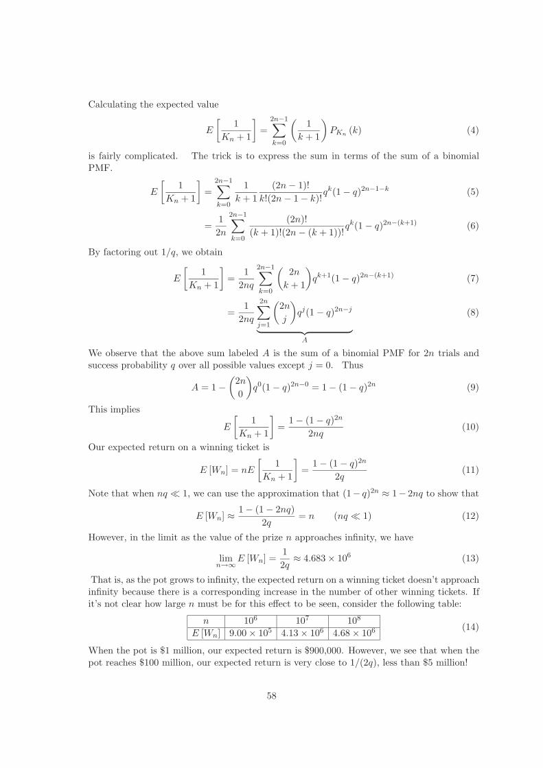
That is, as the pot grows to infinity, the expected return on a winning ticket doesn’t approachinfinity because there is a corresponding increase in the number of other winning tickets. Ifit’s not clear how large n must be for this effect to be seen, consider the following table:
n 106 107 108
E [Wn] 9.00 × 10⁵ 4.13 × 10⁶ 4.68 × 10⁶ (14)
When the pot is $1 million, our expected return is $900,000. However, we see that when thepot reaches $100 million, our expected return is very close to 1/(2q), less than $5 million!
58
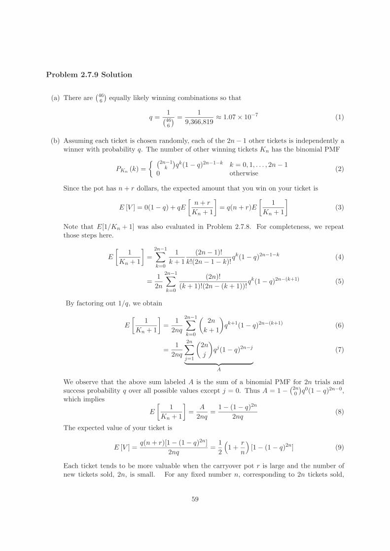
Problem 2.7.9 Solution
(a) There are(466
)equally likely winning combinations so that
q =1(466
) =1
9,366,819≈ 1.07 × 10⁻⁷ (1)
(b) Assuming each ticket is chosen randomly, each of the 2n − 1 other tickets is independently awinner with probability q. The number of other winning tickets Kn has the binomial PMF
PKn (k) ={ (
2n−1k
)qk(1 − q)2n−1−k k = 0, 1, . . . , 2n − 1
0 otherwise(2)
Since the pot has n + r dollars, the expected amount that you win on your ticket is
E [V ] = 0(1 − q) + qE
[n + r
Kn + 1
]= q(n + r)E
[1
Kn + 1
](3)
Note that E[1/Kn + 1] was also evaluated in Problem 2.7.8. For completeness, we repeatthose steps here.
E
[1
Kn + 1
]=
2n−1∑k=0
1k + 1
(2n − 1)!k!(2n − 1 − k)!
qk(1 − q)2n−1−k (4)
=12n
2n−1∑k=0
(2n)!(k + 1)!(2n − (k + 1))!
qk(1 − q)2n−(k+1) (5)
By factoring out 1/q, we obtain
E
[1
Kn + 1
]=
12nq
2n−1∑k=0
(2n
k + 1
)qk+1(1 − q)2n−(k+1) (6)
=1
2nq
2n∑j=1
(2n
j
)qj(1 − q)2n−j
︸ ︷︷ ︸A
(7)
We observe that the above sum labeled A is the sum of a binomial PMF for 2n trials andsuccess probability q over all possible values except j = 0. Thus A = 1 − (2n
0
)q0(1 − q)2n−0,
which implies
E
[1
Kn + 1
]=
A
2nq=
1 − (1 − q)2n
2nq(8)
The expected value of your ticket is
E [V ] =q(n + r)[1 − (1 − q)2n]
2nq=
12
(1 +
r
n
)[1 − (1 − q)2n] (9)
Each ticket tends to be more valuable when the carryover pot r is large and the number ofnew tickets sold, 2n, is small. For any fixed number n, corresponding to 2n tickets sold,
59
a sufficiently large pot r will guarantee that E[V ] > 1. For example if n = 107, (20 milliontickets sold) then
E [V ] = 0.44(1 +
r
107
)(10)
If the carryover pot r is 30 million dollars, then E[V ] = 1.76. This suggests that buying aone dollar ticket is a good idea. This is an unusual situation because normally a carryoverpot of 30 million dollars will result in far more than 20 million tickets being sold.
(c) So that we can use the results of the previous part, suppose there were 2n − 1 tickets soldbefore you must make your decision. If you buy one of each possible ticket, you are guaranteedto have one winning ticket. From the other 2n − 1 tickets, there will be Kn winners. Thetotal number of winning tickets will be Kn + 1. In the previous part we found that
E
[1
Kn + 1
]=
1 − (1 − q)2n
2nq(11)
Let R denote the expected return from buying one of each possible ticket. The pot hadr dollars beforehand. The 2n − 1 other tickets are sold add n − 1/2 dollars to the pot.Furthermore, you must buy 1/q tickets, adding 1/(2q) dollars to the pot. Since the cost ofthe tickets is 1/q dollars, your expected profit
E [R] = E
[r + n − 1/2 + 1/(2q)
Kn + 1
]− 1
q(12)
=q(2r + 2n − 1) + 1
2qE
[1
Kn + 1
]− 1
q(13)
=[q(2r + 2n − 1) + 1](1 − (1 − q)2n)
4nq2− 1
q(14)
For fixed n, sufficiently large r will make E[R] > 0. On the other hand, for fixed r,limn→∞ E[R] = −1/(2q). That is, as n approaches infinity, your expected loss will be quitelarge.
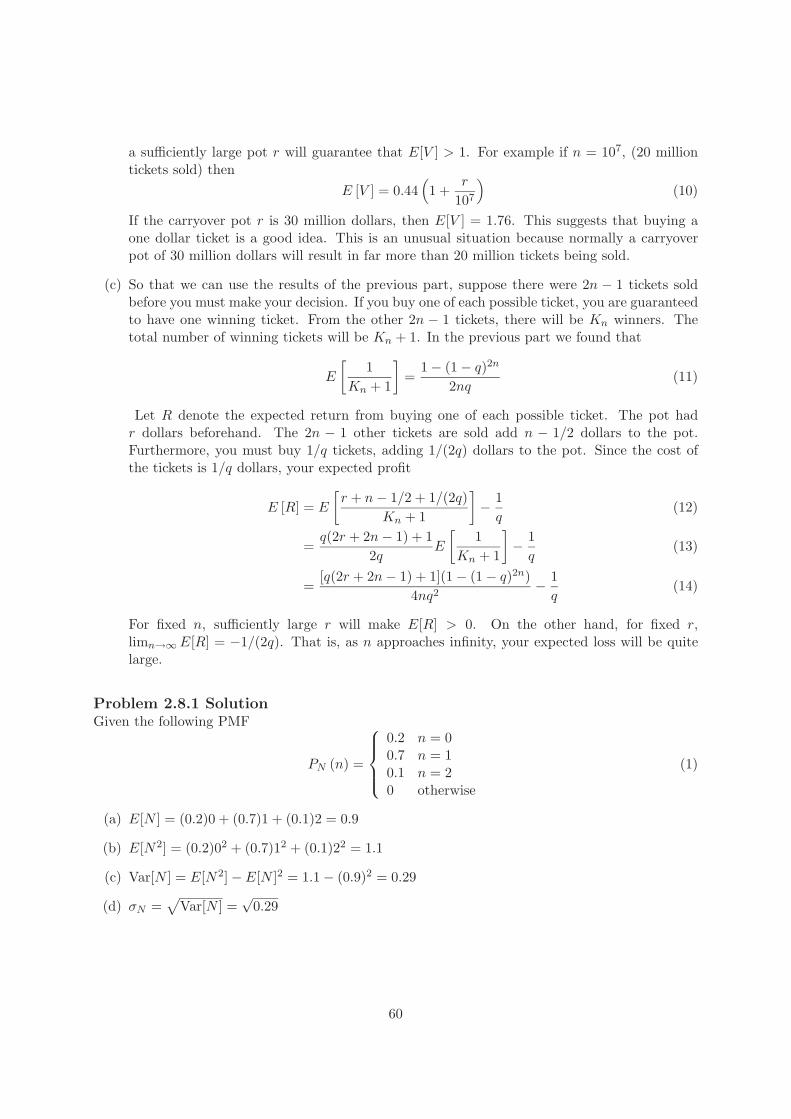
Problem 2.8.1 SolutionGiven the following PMF
PN (n) =
⎧⎪⎪⎨⎪⎪⎩
0.2 n = 00.7 n = 10.1 n = 20 otherwise
(1)
(a) E[N ] = (0.2)0 + (0.7)1 + (0.1)2 = 0.9
(b) E[N2] = (0.2)02 + (0.7)12 + (0.1)22 = 1.1
(c) Var[N ] = E[N2] − E[N ]2 = 1.1 − (0.9)2 = 0.29
(d) σN =√
Var[N ] =√
0.29
60
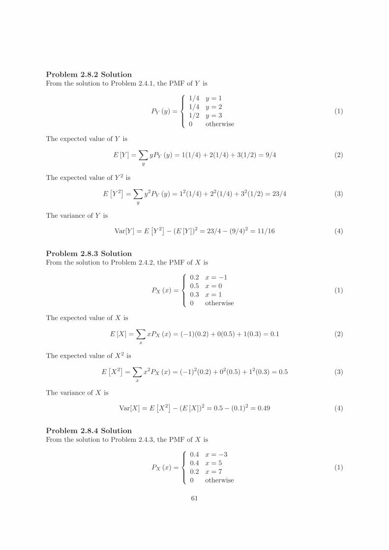
Problem 2.8.2 SolutionFrom the solution to Problem 2.4.1, the PMF of Y is
PY (y) =
⎧⎪⎪⎨⎪⎪⎩
1/4 y = 11/4 y = 21/2 y = 30 otherwise
(1)
The expected value of Y is
E [Y ] =∑
y
yPY (y) = 1(1/4) + 2(1/4) + 3(1/2) = 9/4 (2)
The expected value of Y 2 is
E[Y 2]
=∑
y
y2PY (y) = 12(1/4) + 22(1/4) + 32(1/2) = 23/4 (3)
The variance of Y is
Var[Y ] = E[Y 2]− (E [Y ])2 = 23/4 − (9/4)2 = 11/16 (4)
Problem 2.8.3 SolutionFrom the solution to Problem 2.4.2, the PMF of X is
PX (x) =
⎧⎪⎪⎨⎪⎪⎩
0.2 x = −10.5 x = 00.3 x = 10 otherwise
(1)
The expected value of X is
E [X] =∑
x
xPX (x) = (−1)(0.2) + 0(0.5) + 1(0.3) = 0.1 (2)
The expected value of X2 is
E[X2]
=∑
x
x2PX (x) = (−1)2(0.2) + 02(0.5) + 12(0.3) = 0.5 (3)
The variance of X is
Var[X] = E[X2]− (E [X])2 = 0.5 − (0.1)2 = 0.49 (4)
Problem 2.8.4 SolutionFrom the solution to Problem 2.4.3, the PMF of X is
PX (x) =
⎧⎪⎪⎨⎪⎪⎩
0.4 x = −30.4 x = 50.2 x = 70 otherwise
(1)
61
The expected value of X is
E [X] =∑
x
xPX (x) = −3(0.4) + 5(0.4) + 7(0.2) = 2.2 (2)
The expected value of X2 is
E[X2]
=∑
x
x2PX (x) = (−3)2(0.4) + 52(0.4) + 72(0.2) = 23.4 (3)
The variance of X is
Var[X] = E[X2]− (E [X])2 = 23.4 − (2.2)2 = 18.56 (4)
Problem 2.8.5 Solution
(a) The expected value of X is
E [X] =4∑
x=0
xPX (x) = 0(
40
)124
+ 1(
41
)124
+ 2(
42
)124
+ 3(
43
)124
+ 4(
44
)124
(1)
= [4 + 12 + 12 + 4]/24 = 2 (2)
The expected value of X2 is
E[X2]
=4∑
x=0
x2PX (x) = 02
(40
)124
+ 12
(41
)124
+ 22
(42
)124
+ 32
(43
)124
+ 42
(44
)124
(3)
= [4 + 24 + 36 + 16]/24 = 5 (4)
The variance of X isVar[X] = E
[X2]− (E [X])2 = 5 − 22 = 1 (5)
Thus, X has standard deviation σX =√
Var[X] = 1.
(b) The probability that X is within one standard deviation of its expected value is
P [μX − σX ≤ X ≤ μX + σX ] = P [2 − 1 ≤ X ≤ 2 + 1] = P [1 ≤ X ≤ 3] (6)
This calculation is easy using the PMF of X.
P [1 ≤ X ≤ 3] = PX (1) + PX (2) + PX (3) = 7/8 (7)
Problem 2.8.6 Solution
(a) The expected value of X is
E [X] =5∑
x=0
xPX (x) (1)
= 0(
50
)125
+ 1(
51
)125
+ 2(
52
)125
+ 3(
53
)125
+ 4(
54
)125
+ 5(
55
)125
(2)
= [5 + 20 + 30 + 20 + 5]/25 = 5/2 (3)
62

The expected value of X2 is
E[X2]
=5∑
x=0
x2PX (x) (4)
= 02
(50
)125
+ 12
(51
)125
+ 22
(52
)125
+ 32
(53
)125
+ 42
(54
)125
+ 52
(55
)125
(5)
= [5 + 40 + 90 + 80 + 25]/25 = 240/32 = 15/2 (6)
The variance of X is
Var[X] = E[X2]− (E [X])2 = 15/2 − 25/4 = 5/4 (7)
By taking the square root of the variance, the standard deviation of X is σX =√
5/4 ≈ 1.12.
(b) The probability that X is within one standard deviation of its mean is
P [μX − σX ≤ X ≤ μX + σX ] = P [2.5 − 1.12 ≤ X ≤ 2.5 + 1.12] (8)= P [1.38 ≤ X ≤ 3.62] (9)= P [2 ≤ X ≤ 3] (10)
By summing the PMF over the desired range, we obtain
P [2 ≤ X ≤ 3] = PX (2) + PX (3) = 10/32 + 10/32 = 5/8 (11)
Problem 2.8.7 SolutionFor Y = aX + b, we wish to show that Var[Y ] = a2 Var[X]. We begin by noting that Theorem 2.12says that E[aX + b] = aE[X] + b. Hence, by the definition of variance.
Var [Y ] = E[(aX + b − (aE [X] + b))2
](1)
= E[a2(X − E [X])2
](2)
= a2E[(X − E [X])2
](3)
Since E[(X − E[X])2] = Var[X], the assertion is proved.
Problem 2.8.8 SolutionGiven the following description of the random variable Y ,
Y =1σx
(X − μX) (1)
we can use the linearity property of the expectation operator to find the mean value
E [Y ] =E [X − μX ]
σX=
E [X] − E [X]σX
= 0 (2)
Using the fact that Var[aX + b] = a2 Var[X], the variance of Y is found to be
Var [Y ] =1
σ2X
Var [X] = 1 (3)
63
Problem 2.8.9 SolutionWith our measure of jitter being σT , and the fact that T = 2X − 1, we can express the jitter as afunction of q by realizing that
Var[T ] = 4 Var[X] =4q
(1 − q)2(1)
Therefore, our maximum permitted jitter is
σT =2√
q
(1 − q)= 2 msec (2)
Solving for q yields q2 − 3q + 1 = 0. By solving this quadratic equation, we obtain
q =3 ±√
52
= 3/2 ±√
5/2 (3)
Since q must be a value between 0 and 1, we know that a value of q = 3/2 − √5/2 ≈ 0.382 will
ensure a jitter of at most 2 milliseconds.
Problem 2.8.10 SolutionWe wish to minimize the function
e(x̂) = E[(X − x̂)2
](1)
with respect to x̂. We can expand the square and take the expectation while treating x̂ as aconstant. This yields
e(x̂) = E[X2 − 2x̂X + x̂2
]= E
[X2]− 2x̂E [X] + x̂2 (2)
Solving for the value of x̂ that makes the derivative de(x̂)/dx̂ equal to zero results in the value ofx̂ that minimizes e(x̂). Note that when we take the derivative with respect to x̂, both E[X2] andE[X] are simply constants.
d
dx̂
(E[X2]− 2x̂E [X] + x̂2
)= 2E [X] − 2x̂ = 0 (3)
Hence we see that x̂ = E[X]. In the sense of mean squared error, the best guess for a randomvariable is the mean value. In Chapter 9 this idea is extended to develop minimum mean squarederror estimation.
Problem 2.8.11 SolutionThe PMF of K is the Poisson PMF
PK (k) ={
λke−λ/k! k = 0, 1, . . .0 otherwise
(1)
The mean of K is
E [K] =∞∑
k=0
kλke−λ
k!= λ
∞∑k=1
λk−1e−λ
(k − 1)!= λ (2)
To find E[K2], we use the hint and first find
E [K(K − 1)] =∞∑
k=0
k(k − 1)λke−λ
k!=
∞∑k=2
λke−λ
(k − 2)!(3)
64
By factoring out λ2 and substituting j = k − 2, we obtain
E [K(K − 1)] = λ2∞∑
j=0
λje−λ
j!︸ ︷︷ ︸1
= λ2 (4)
The above sum equals 1 because it is the sum of a Poisson PMF over all possible values. SinceE[K] = λ, the variance of K is
Var[K] = E[K2]− (E [K])2 (5)
= E [K(K − 1)] + E [K] − (E [K])2 (6)
= λ2 + λ − λ2 = λ (7)
Problem 2.8.12 SolutionThe standard deviation can be expressed as
σD =√
Var[D] =√
E [D2] − E [D]2 (1)
where
E[D2]
=4∑
d=1
d2PD(d) = 0.2 + 1.6 + 2.7 + 1.6 = 6.1 (2)
So finally we haveσD =
√6.1 − 2.32 =
√0.81 = 0.9 (3)
Problem 2.9.1 SolutionFrom the solution to Problem 2.4.1, the PMF of Y is
PY (y) =
⎧⎪⎪⎨⎪⎪⎩
1/4 y = 11/4 y = 21/2 y = 30 otherwise
(1)
The probability of the event B = {Y < 3} is P [B] = 1−P [Y = 3] = 1/2. From Theorem 2.17, theconditional PMF of Y given B is
PY |B (y) =
{PY (y)P [B] y ∈ B
0 otherwise=
⎧⎨⎩
1/2 y = 11/2 y = 20 otherwise
(2)
The conditional first and second moments of Y are
E [Y |B] =∑
y
yPY |B (y) = 1(1/2) + 2(1/2) = 3/2 (3)
E[Y 2|B] =
∑y
y2PY |B (y) = 12(1/2) + 22(1/2) = 5/2 (4)
The conditional variance of Y is
Var[Y |B] = E[Y 2|B]− (E [Y |B])2 = 5/2 − 9/4 = 1/4 (5)
65
Problem 2.9.2 SolutionFrom the solution to Problem 2.4.2, the PMF of X is
PX (x) =
⎧⎪⎪⎨⎪⎪⎩
0.2 x = −10.5 x = 00.3 x = 10 otherwise
(1)
The event B = {|X| > 0} has probability P [B] = P [X = 0] = 0.5. From Theorem 2.17, theconditional PMF of X given B is
PX|B (x) =
{PX(x)P [B] x ∈ B
0 otherwise=
⎧⎨⎩
0.4 x = −10.6 x = 10 otherwise
(2)
The conditional first and second moments of X are
E [X|B] =∑
x
xPX|B (x) = (−1)(0.4) + 1(0.6) = 0.2 (3)
E[X2|B] =
∑x
x2PX|B (x) = (−1)2(0.4) + 12(0.6) = 1 (4)
The conditional variance of X is
Var[X|B] = E[X2|B]− (E [X|B])2 = 1 − (0.2)2 = 0.96 (5)
Problem 2.9.3 SolutionFrom the solution to Problem 2.4.3, the PMF of X is
PX (x) =
⎧⎪⎪⎨⎪⎪⎩
0.4 x = −30.4 x = 50.2 x = 70 otherwise
(1)
The event B = {X > 0} has probability P [B] = PX(5) + PX(7) = 0.6. From Theorem 2.17, theconditional PMF of X given B is
PX|B (x) =
{PX(x)P [B] x ∈ B
0 otherwise=
⎧⎨⎩
2/3 x = 51/3 x = 70 otherwise
(2)
The conditional first and second moments of X are
E [X|B] =∑
x
xPX|B (x) = 5(2/3) + 7(1/3) = 17/3 (3)
E[X2|B] =
∑x
x2PX|B (x) = 52(2/3) + 72(1/3) = 33 (4)
The conditional variance of X is
Var[X|B] = E[X2|B]− (E [X|B])2 = 33 − (17/3)2 = 8/9 (5)
66

Problem 2.9.4 SolutionThe event B = {X = 0} has probability P [B] = 1 − P [X = 0] = 15/16. The conditional PMF ofX given B is
PX|B (x) =
{PX(x)P [B] x ∈ B
0 otherwise={ (
4x
)115 x = 1, 2, 3, 4
0 otherwise(1)
The conditional first and second moments of X are
E [X|B] =4∑
x=1
xPX|B (x) = 1(
41
)115
2(
42
)115
+ 3(
43
)115
+ 4(
44
)115
(2)
= [4 + 12 + 12 + 4]/15 = 32/15 (3)
E[X2|B] =
4∑x=1
x2PX|B (x) = 12
(41
)115
22
(42
)115
+ 32
(43
)115
+ 42
(44
)115
(4)
= [4 + 24 + 36 + 16]/15 = 80/15 (5)
The conditional variance of X is
Var[X|B] = E[X2|B]− (E [X|B])2 = 80/15 − (32/15)2 = 176/225 ≈ 0.782 (6)
Problem 2.9.5 SolutionThe probability of the event B is
P [B] = P [X ≥ μX ] = P [X ≥ 3] = PX (3) + PX (4) + PX (5) (1)
=
(53
)+(54
)+(55
)32
= 21/32 (2)
The conditional PMF of X given B is
PX|B (x) =
{PX(x)P [B] x ∈ B
0 otherwise={ (
5x
)121 x = 3, 4, 5
0 otherwise(3)
The conditional first and second moments of X are
E [X|B] =5∑
x=3
xPX|B (x) = 3(
53
)121
+ 4(
54
)121
+ 5(
55
)121
(4)
= [30 + 20 + 5]/21 = 55/21 (5)
E[X2|B] =
5∑x=3
x2PX|B (x) = 32
(53
)121
+ 42
(54
)121
+ 52
(55
)121
(6)
= [90 + 80 + 25]/21 = 195/21 = 65/7 (7)
The conditional variance of X is
Var[X|B] = E[X2|B]− (E [X|B])2 = 65/7 − (55/21)2 = 1070/441 = 2.43 (8)
67
Problem 2.9.6 Solution
(a) Consider each circuit test as a Bernoulli trial such that a failed circuit is called a success.The number of trials until the first success (i.e. a failed circuit) has the geometric PMF
PN (n) ={
(1 − p)n−1p n = 1, 2, . . .0 otherwise
(1)
(b) The probability there are at least 20 tests is
P [B] = P [N ≥ 20] =∞∑
n=20
PN (n) = (1 − p)19 (2)
Note that (1 − p)19 is just the probability that the first 19 circuits pass the test, which iswhat we would expect since there must be at least 20 tests if the first 19 circuits pass. Theconditional PMF of N given B is
PN |B (n) =
{PN (n)P [B] n ∈ B
0 otherwise={
(1 − p)n−20p n = 20, 21, . . .0 otherwise
(3)
(c) Given the event B, the conditional expectation of N is
E [N |B] =∑
n
nPN |B (n) =∞∑
n=20
n(1 − p)n−20p (4)
Making the substitution j = n − 19 yields
E [N |B] =∞∑
j=1
(j + 19)(1 − p)j−1p = 1/p + 19 (5)
We see that in the above sum, we effectively have the expected value of J + 19 where J isgeometric random variable with parameter p. This is not surprising since the N ≥ 20 iff weobserved 19 successful tests. After 19 successful tests, the number of additional tests neededto find the first failure is still a geometric random variable with mean 1/p.
Problem 2.9.7 Solution
(a) The PMF of M , the number of miles run on an arbitrary day is
PM (m) ={
q(1 − q)m m = 0, 1, . . .0 otherwise
(1)
And we can see that the probability that M > 0, is
P [M > 0] = 1 − P [M = 0] = 1 − q (2)
68

(b) The probability that we run a marathon on any particular day is the probability that M ≥ 26.
r = P [M ≥ 26] =∞∑
m=26
q(1 − q)m = (1 − q)26 (3)
(c) We run a marathon on each day with probability equal to r, and we do not run a marathonwith probability 1− r. Therefore in a year we have 365 tests of our jogging resolve, and thus365 chances to run a marathon. So the PMF of the number of marathons run in a year, J ,can be expressed as
PJ (j) ={ (
365j
)rj(1 − r)365−j j = 0, 1, . . . , 365
0 otherwise(4)
(d) The random variable K is defined as the number of miles we run above that required for amarathon, K = M − 26. Given the event, A, that we have run a marathon, we wish to knowhow many miles in excess of 26 we in fact ran. So we want to know the conditional PMFPK|A(k).
PK|A (k) =P [K = k, A]
P [A]=
P [M = 26 + k]P [A]
(5)
Since P [A] = r, for k = 0, 1, . . .,
PK|A (k) =(1 − q)26+kq
(1 − q)26= (1 − q)kq (6)
The complete expression of for the conditional PMF of K is
PK|A (k) ={
(1 − q)kq k = 0, 1, . . .0 otherwise
(7)
Problem 2.9.8 SolutionRecall that the PMF of the number of pages in a fax is
PX (x) =
⎧⎨⎩
0.15 x = 1, 2, 3, 40.1 x = 5, 6, 7, 80 otherwise
(1)
(a) The event that a fax was sent to machine A can be expressed mathematically as the eventthat the number of pages X is an even number. Similarly, the event that a fax was sentto B is the event that X is an odd number. Since SX = {1, 2, . . . , 8}, we define the setA = {2, 4, 6, 8}. Using this definition for A, we have that the event that a fax is sent to A isequivalent to the event X ∈ A. The event A has probability
P [A] = PX (2) + PX (4) + PX (6) + PX (8) = 0.5 (2)
Given the event A, the conditional PMF of X is
PX|A (x) =
{PX(x)P [A] x ∈ A
0 otherwise=
⎧⎨⎩
0.3 x = 2, 40.2 x = 6, 80 otherwise
(3)
69

The conditional first and second moments of X given A is
E [X|A] =∑
x
xPX|A (x) = 2(0.3) + 4(0.3) + 6(0.2) + 8(0.2) = 4.6 (4)
E[X2|A] =
∑x
x2PX|A (x) = 4(0.3) + 16(0.3) + 36(0.2) + 64(0.2) = 26 (5)
The conditional variance and standard deviation are
Var[X|A] = E[X2|A]− (E [X|A])2 = 26 − (4.6)2 = 4.84 (6)
σX|A =√
Var[X|A] = 2.2 (7)
(b) Let the event B′ denote the event that the fax was sent to B and that the fax had no morethan 6 pages. Hence, the event B′ = {1, 3, 5} has probability
P[B′] = PX (1) + PX (3) + PX (5) = 0.4 (8)
The conditional PMF of X given B′ is
PX|B′ (x) =
{PX(x)P [B′] x ∈ B′
0 otherwise=
⎧⎨⎩
3/8 x = 1, 31/4 x = 50 otherwise
(9)
Given the event B′, the conditional first and second moments are
E[X|B′] =
∑x
xPX|B′ (x) = 1(3/8) + 3(3/8) + 5(1/4)+ = 11/4 (10)
E[X2|B′] =
∑x
x2PX|B′ (x) = 1(3/8) + 9(3/8) + 25(1/4) = 10 (11)
The conditional variance and standard deviation are
Var[X|B′] = E[X2|B′]− (E
[X|B′])2 = 10 − (11/4)2 = 39/16 (12)
σX|B′ =√
Var[X|B′] =√
39/4 ≈ 1.56 (13)
Problem 2.10.1 SolutionFor a binomial (n, p) random variable X, the solution in terms of math is
P [E2] =�√n�∑x=0
PX
(x2)
(1)
In terms of Matlab, the efficient solution is to generate the vector of perfect squares x =[0 1 4 9 16 ...] and then to pass that vector to the binomialpmf.m. In this case, the val-ues of the binomial PMF are calculated only once. Here is the code:
function q=perfectbinomial(n,p);i=0:floor(sqrt(n));x=i.^2;q=sum(binomialpmf(n,p,x));
For a binomial (100, 0.5) random variable X, the probability X is a perfect square is>> perfectbinomial(100,0.5)ans =
0.0811
70
Problem 2.10.2 SolutionThe random variable X given in Example 2.29 is just a finite random variable. We can generaterandom samples using the finiterv function. The code is
function x=faxlength8(m);sx=1:8;p=[0.15*ones(1,4) 0.1*ones(1,4)];x=finiterv(sx,p,m);
Problem 2.10.3 SolutionFirst we use faxlength8 from Problem 2.10.2 to generate m samples of the faqx length X. Nextwe convert that to m samples of the fax cost Y . Summing these samples and dividing by m, weobtain the average cost of m samples. Here is the code:
function y=avgfax(m);x=faxlength8(m);yy=cumsum([10 9 8 7 6]);yy=[yy 50 50 50];y=sum(yy(x))/m;
Each time we perform the experiment of executing the function avgfax, we generate m randomsamples of X, and m corresponding samples of Y . The sum Y = 1
m
∑mi=1 Yi is random. For m = 10,
four samples of Y are
>> [avgfax(10) avgfax(10) avgfax(10) avgfax(10)]ans =
31.9000 31.2000 29.6000 34.1000>>
For m = 100, the results are arguably more consistent:
>> [avgfax(100) avgfax(100) avgfax(100) avgfax(100)]ans =
34.5300 33.3000 29.8100 33.6900>>
Finally, for m = 1000, we obtain results reasonably close to E[Y ]:
>> [avgfax(1000) avgfax(1000) avgfax(1000) avgfax(1000)]ans =
32.1740 31.8920 33.1890 32.8250>>
In Chapter 7, we will develop techniques to show how Y converges to E[Y ] as m → ∞.
Problem 2.10.4 SolutionSuppose Xn is a Zipf (n, α = 1) random variable and thus has PMF
PX (x) ={
c(n)/x x = 1, 2, . . . , n0 otherwise
(1)
The problem asks us to find the smallest value of k such that P [Xn ≤ k] ≥ 0.75. That is, if theserver caches the k most popular files, then with P [Xn ≤ k] the request is for one of the k cached
71
files. First, we might as well solve this problem for any probability p rather than just p = 0.75.Thus, in math terms, we are looking for
k = min{k′|P [Xn ≤ k′] ≥ p
}. (2)
What makes the Zipf distribution hard to analyze is that there is no closed form expression for
c(n) =
(n∑
x=1
1x
)−1
. (3)
Thus, we use Matlab to grind through the calculations. The following simple program generatesthe Zipf distributions and returns the correct value of k.
function k=zipfcache(n,p);%Usage: k=zipfcache(n,p);%for the Zipf (n,alpha=1) distribution, returns the smallest k%such that the first k items have total probability ppmf=1./(1:n);pmf=pmf/sum(pmf); %normalize to sum to 1cdf=cumsum(pmf);k=1+sum(cdf<=p);
The program zipfcache generalizes 0.75 to be the probability p. Although this program is suffi-cient, the problem asks us to find k for all values of n from 1 to 103!. One way to do this is to callzipfcache a thousand times to find k for each value of n. A better way is to use the properties ofthe Zipf PDF. In particular,
P[Xn ≤ k′] = c(n)
k′∑x=1
1x
=c(n)c(k′)
(4)
Thus we wish to find
k = min{
k′| c(n)c(k′)
≥ p
}= min
{k′| 1
c(k′)≥ p
c(n)
}. (5)
Note that the definition of k implies that
1c(k′)
<p
c(n), k′ = 1, . . . , k − 1. (6)
Using the notation |A| to denote the number of elements in the set A, we can write
k = 1 +∣∣∣∣{
k′| 1c(k′)
<p
c(n)
}∣∣∣∣ (7)
This is the basis for a very short Matlab program:
function k=zipfcacheall(n,p);%Usage: k=zipfcacheall(n,p);%returns vector k such that the first%k(m) items have total probability >= p%for the Zipf(m,1) distribution.c=1./cumsum(1./(1:n));k=1+countless(1./c,p./c);
72
Note that zipfcacheall uses a short Matlab program countless.m that is almost the same ascount.m introduced in Example 2.47. If n=countless(x,y), then n(i) is the number of elementsof x that are strictly less than y(i) while count returns the number of elements less than or equalto y(i).
In any case, the commands
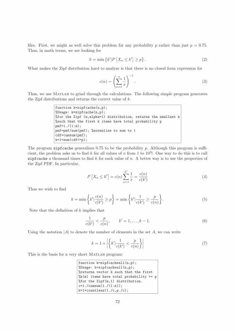
k=zipfcacheall(1000,0.75);plot(1:1000,k);
is sufficient to produce this figure of k as a function of m:
0 100 200 300 400 500 600 700 800 900 10000
50
100
150
200
n
k
We see in the figure that the number of files that must be cached grows slowly with the totalnumber of files n.
Finally, we make one last observation. It is generally desirable for Matlab to execute opera-tions in parallel. The program zipfcacheall generally will run faster than n calls to zipfcache.However, to do its counting all at once, countless generates and n × n array. When n is not toolarge, say n ≤ 1000, the resulting array with n2 = 1,000,000 elements fits in memory. For muchlarge values of n, say n = 106 (as was proposed in the original printing of this edition of the text,countless will cause an “out of memory” error.
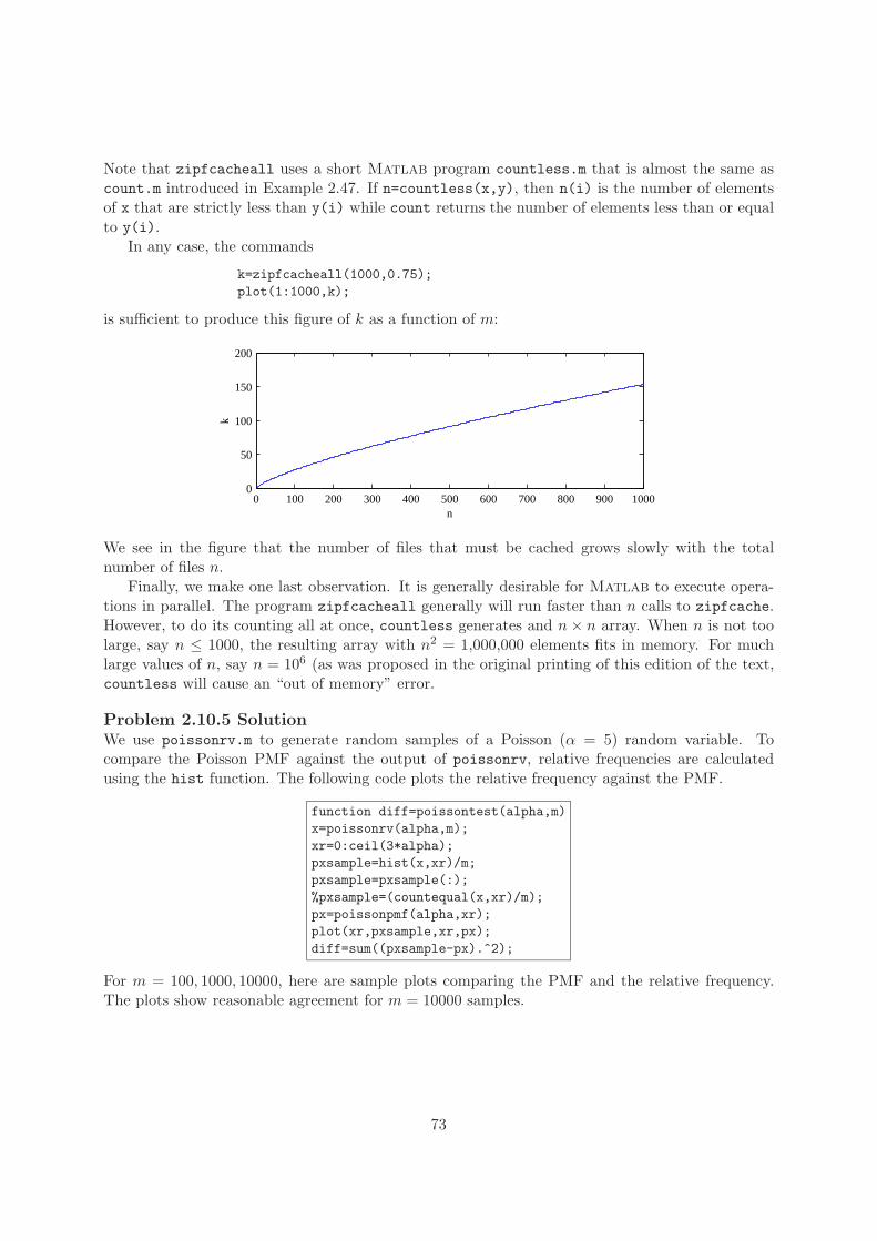
Problem 2.10.5 SolutionWe use poissonrv.m to generate random samples of a Poisson (α = 5) random variable. Tocompare the Poisson PMF against the output of poissonrv, relative frequencies are calculatedusing the hist function. The following code plots the relative frequency against the PMF.
function diff=poissontest(alpha,m)x=poissonrv(alpha,m);xr=0:ceil(3*alpha);pxsample=hist(x,xr)/m;pxsample=pxsample(:);%pxsample=(countequal(x,xr)/m);px=poissonpmf(alpha,xr);plot(xr,pxsample,xr,px);diff=sum((pxsample-px).^2);
For m = 100, 1000, 10000, here are sample plots comparing the PMF and the relative frequency.The plots show reasonable agreement for m = 10000 samples.
73

0 5 10 150
0.1
0.2
0 5 10 150
0.1
0.2
(a) m = 100 (b) m = 100
0 5 10 150
0.1
0.2
0 5 10 150
0.1
0.2
(a) m = 1000 (b) m = 1000
0 5 10 150
0.1
0.2
0 5 10 150
0.1
0.2
(a) m = 10,000 (b) m = 10,000
Problem 2.10.6 SolutionWe can compare the binomial and Poisson PMFs for (n, p) = (100, 0.1) using the following Matlabcode:
x=0:20;p=poissonpmf(100,x);b=binomialpmf(100,0.1,x);plot(x,p,x,b);
For (n, p) = (10, 1), the binomial PMF has no randomness. For (n, p) = (100, 0.1), the approxima-tion is reasonable:
0 5 10 15 200
0.2
0.4
0.6
0.8
1
0 5 10 15 200
0.05
0.1
0.15
0.2
(a) n = 10, p = 1 (b) n = 100, p = 0.1
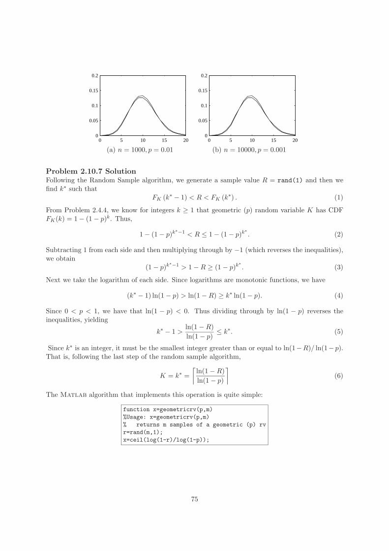
Finally, for (n, p) = (1000, 0.01), and (n, p) = (10000, 0.001), the approximation is very good:
74
0 5 10 15 200
0.05
0.1
0.15
0.2
0 5 10 15 200
0.05
0.1
0.15
0.2
(a) n = 1000, p = 0.01 (b) n = 10000, p = 0.001
Problem 2.10.7 SolutionFollowing the Random Sample algorithm, we generate a sample value R = rand(1) and then wefind k∗ such that
FK (k∗ − 1) < R < FK (k∗) . (1)
From Problem 2.4.4, we know for integers k ≥ 1 that geometric (p) random variable K has CDFFK(k) = 1 − (1 − p)k. Thus,
1 − (1 − p)k∗−1 < R ≤ 1 − (1 − p)k∗. (2)
Subtracting 1 from each side and then multiplying through by −1 (which reverses the inequalities),we obtain
(1 − p)k∗−1 > 1 − R ≥ (1 − p)k∗. (3)
Next we take the logarithm of each side. Since logarithms are monotonic functions, we have
(k∗ − 1) ln(1 − p) > ln(1 − R) ≥ k∗ ln(1 − p). (4)
Since 0 < p < 1, we have that ln(1 − p) < 0. Thus dividing through by ln(1 − p) reverses theinequalities, yielding
k∗ − 1 >ln(1 − R)ln(1 − p)
≤ k∗. (5)
Since k∗ is an integer, it must be the smallest integer greater than or equal to ln(1−R)/ ln(1− p).That is, following the last step of the random sample algorithm,
K = k∗ =⌈
ln(1 − R)ln(1 − p)
⌉(6)
The Matlab algorithm that implements this operation is quite simple:
function x=geometricrv(p,m)%Usage: x=geometricrv(p,m)% returns m samples of a geometric (p) rvr=rand(m,1);x=ceil(log(1-r)/log(1-p));
75

Problem 2.10.8 SolutionFor the PC version of Matlab employed for this test, poissonpmf(n,n) reported Inf for n =n∗ = 714. The problem with the poissonpmf function in Example 2.44 is that the cumulativeproduct that calculated nk/k! can have an overflow. Following the hint, we can write an alternatepoissonpmf function as follows:
function pmf=poissonpmf(alpha,x)%Poisson (alpha) rv X,%out=vector pmf: pmf(i)=P[X=x(i)]x=x(:);if (alpha==0)
pmf=1.0*(x==0);else
k=(1:ceil(max(x)))’;logfacts =cumsum(log(k));pb=exp([-alpha; ...
-alpha+ (k*log(alpha))-logfacts]);okx=(x>=0).*(x==floor(x));x=okx.*x;pmf=okx.*pb(x+1);
end%pmf(i)=0 for zero-prob x(i)
By summing logarithms, the intermediate terms are much less likely to overflow.
76