problem description - adina description ... stations along the crack front. actual crack propagation...

Problem 17: Analysis of a cracked body with ADINA-M/PS

ADINA R & D, Inc. 17-1

Problem description It is desired to analyze the cracked body shown using a 3D finite element mesh:

30

30

30 radius35 radius

50 radius

Cracked body dimensions

Top view

100

50

27.5

27.5

All dimensions in mm

Front view

10 N vertical loadapplied to top holes

6

Bottom holes fixed

Material properties:

E = 2.07 10 N/mm�5 2

� = 0.29

Crack front line

Crack front line


17-2 ADINA Primer

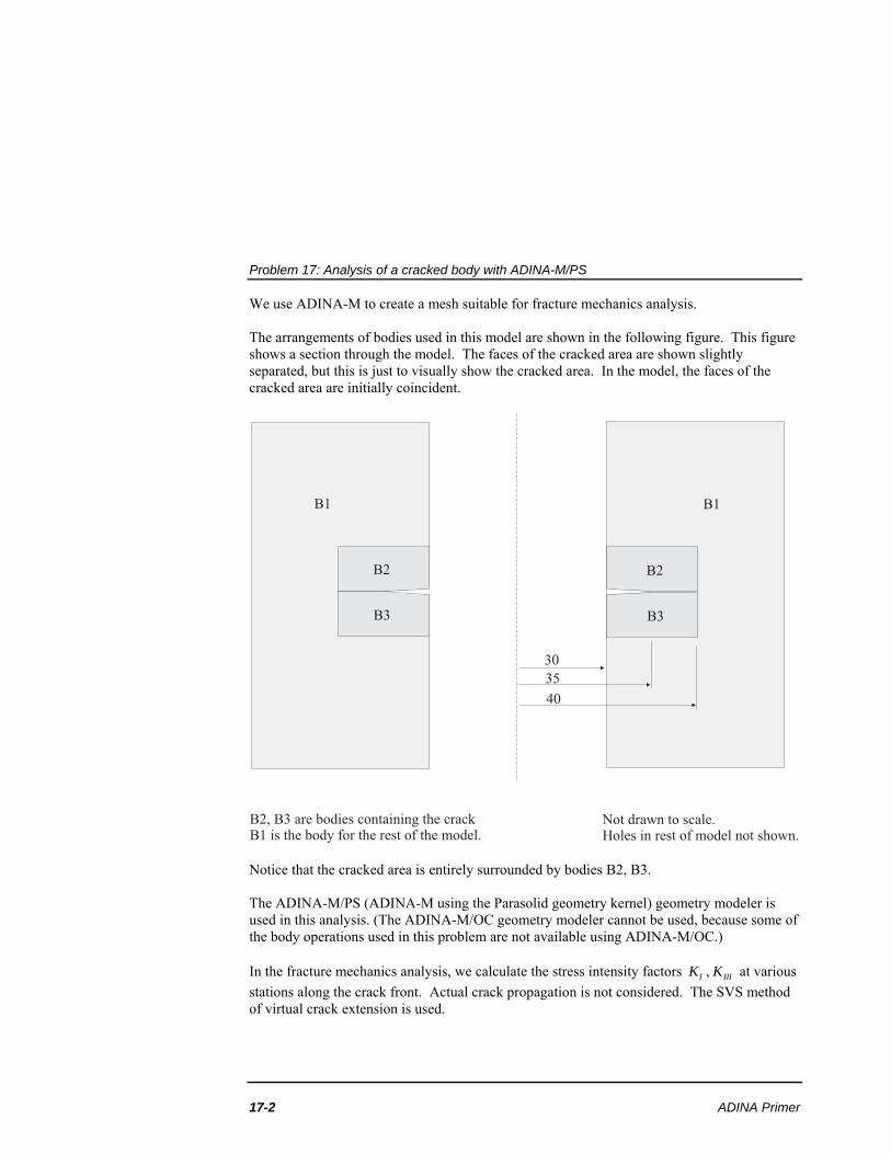
We use ADINA-M to create a mesh suitable for fracture mechanics analysis. The arrangements of bodies used in this model are shown in the following figure. This figure shows a section through the model. The faces of the cracked area are shown slightly separated, but this is just to visually show the cracked area. In the model, the faces of the cracked area are initially coincident.

B2

B3

30

35

40

B1

B2, B3 are bodies containing the crackB1 is the body for the rest of the model.

Not drawn to scale.Holes in rest of model not shown.

B2

B1

B3

Notice that the cracked area is entirely surrounded by bodies B2, B3. The ADINA-M/PS (ADINA-M using the Parasolid geometry kernel) geometry modeler is used in this analysis. (The ADINA-M/OC geometry modeler cannot be used, because some of the body operations used in this problem are not available using ADINA-M/OC.) In the fracture mechanics analysis, we calculate the stress intensity factors IK , IIIK at various

stations along the crack front. Actual crack propagation is not considered. The SVS method of virtual crack extension is used.



For the theory used in fracture mechanics, see Chapter 10 of the ADINA Structures Theory and Modeling Guide. In this problem solution, we will demonstrate the following topics that have not been presented in previous problems: • Projecting a line onto body faces • Linking faces of ADINA-M/PS geometry • Defining constraint sets • Generating free-form meshes with 27-node hexahedral elements • Splitting meshes • Creating CRACK-SVS definitions • Using cutting planes to examine the mesh and the results • Using the fracture mechanics analysis features. Before you begin Please refer to the Icon Locator Tables chapter of the Primer for the locations of all of the AUI icons. Please refer to the Hints chapter of the Primer for useful hints. Note that you must have a version of the AUI that includes the ADINA-M/PS geometry modeler. In addition you need to allocate at least 80 MB of memory to the AUI. This problem cannot be solved with the 900 nodes version of the ADINA System because the model contains more than 900 nodes. Invoking the AUI and choosing the finite element program Invoke the AUI and set the Program Module drop-down list to ADINA Structures. Choose EditMemory Usage and make sure that the ADINA/AUI memory is at least 80 MB. Defining model control data Problem heading: Choose ControlHeading, enter the heading “Problem 17: Analysis of a cracked body with ADINA-M/PS” and click OK. Overview of geometry definition The SVS method of virtual crack extension allows the mesh to be unstructured (free-form) adjacent to the crack front. This has the advantage that fewer steps need to be used in creating the mesh, as compared to the number of steps needed to create a structured mesh. Before proceeding with the geometry definition, we outline with sketches the steps used. You may want to refer to these steps when working through this problem.


17-4 ADINA Primer

Step 1) Define geometry without crack.

x y

Pipe body created

B1

B = body

Top holes created Bottom holes created

z

Step 2) Create crack bodies (bodies that will contain the crack).

B3

B1

Isometric view of bodies 2 and 3 Section view of bodies 1, 2, 3,bodies 2 and 3 overlap body 1,not to scale

B1

B2 B2

B3

B3B2

Step 3) Subtract crack bodies from the body created in step 1.

B3

B1 B1

B2 B2

B3



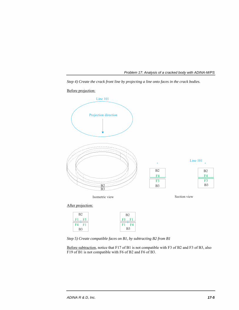
Step 4) Create the crack front line by projecting a line onto faces in the crack bodies. Before projection:

B3

Line 101

Line 101

Projection direction

B2 B2

F4F4

F3F3B3

B3

Isometric view Section view

B2

After projection:

B3

B2 B2

F5F5F1 F1

F1 F1F4 F4B3

Step 5) Create compatible faces on B1, by subtracting B2 from B1 Before subtraction, notice that F17 of B1 is not compatible with F3 of B2 and F3 of B3, also F19 of B1 is not compatible with F6 of B2 and F6 of B3.


17-6 ADINA Primer

F17F19

F4

F5

F1F4 F4

F1 F1

F1

F5

F6

F6

F3

F3

F5 F5

F4

Section view of B1, B2, B3

B3

B1 B1

B2 B2

B3

After subtraction, F1 of B1 is compatible with F3 of B2, F2 of B1 is compatible with F6 of B2, etc.

F1

F19

F2

F21

F4

F5

F1F4 F4

F1 F1

F1

F5

F6

F6

F3

F3

F5 F5

F4

B3

B1 B1

B2 B2

B3

Overview of crack definition In this model, we use the mesh split feature to create duplicate nodes on the cracked faces. Step 1) Split the meshes on B2 and B3, to create duplicate nodes on F5 of B2 and F1 of B3. Before mesh split:

Mesh on B3

Mesh on B2



After mesh split:

Duplicate nodes separated in this figure for clarity,in actual mesh, duplicate nodes overlap

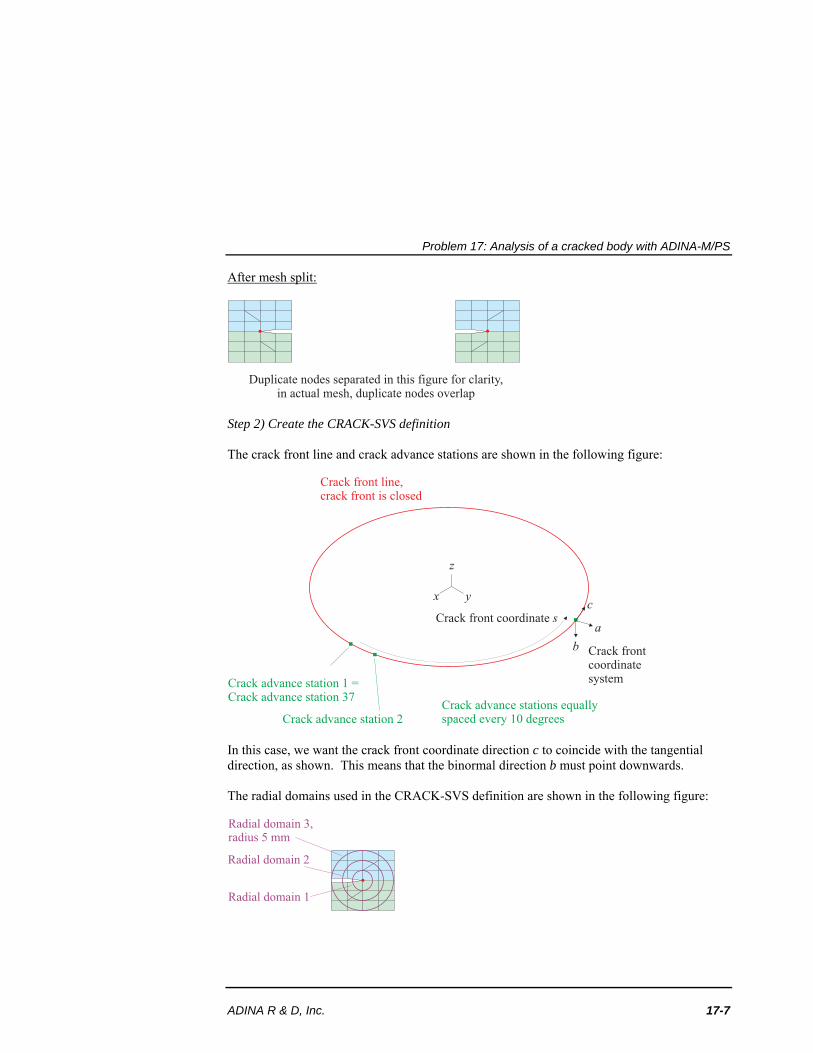
Step 2) Create the CRACK-SVS definition The crack front line and crack advance stations are shown in the following figure:

Crack frontcoordinatesystem

Crack front line,crack front is closed

Crack advance station 1 =Crack advance station 37

Crack advance station 2Crack advance stations equallyspaced every 10 degrees

Crack front coordinate s

x

a

b

cy

z

In this case, we want the crack front coordinate direction c to coincide with the tangential direction, as shown. This means that the binormal direction b must point downwards. The radial domains used in the CRACK-SVS definition are shown in the following figure:

Radial domain 1

Radial domain 2

Radial domain 3,radius 5 mm


17-8 ADINA Primer

Defining geometry, step 1: Define geometry without crack

Pipe: Click the Define Bodies icon , add body 1, set the Type to Pipe, the Outer Radius to 50, the Thickness to 20, the Length to 100, make sure that the Center Position is (0.0, 0.0, 0.0), set the Axis to Z and click Save. (We do not want to close the dialog box yet.) Creation of holes: To make the first set of holes, we create a cylinder and subtract it from the pipe body. Add body 2, set the Type to Cylinder, the Radius to 15, the Length to 150, the Center Position to (0.0, 0.0, 27.5), make sure that the Axis is X and click OK.

Now click the Boolean Operator icon , set the Operator Type to Subtract, set the Target Body to 1, enter 2 in the first row of the table and click OK.

We make the second set of holes in a similar way. Click the Define Bodies icon , add body 2, set the Type to Cylinder, the Radius to 15, the Length to 150, the Center Position to (0.0, 0.0, -27.5), the Axis to Y and click OK.

Now click the Boolean Operator icon , set the Operator Type to Subtract, set the Target Body to 1, enter 2 in the first row of the table and click OK. When you click the Wire Frame

icon , the graphics window should look something like this:

TIME 1.000

X Y

Z



Defining geometry, step 2: Create crack bodies (bodies that will contain the crack)

Click the Define Bodies icon , add body 2, set the Type to Pipe, the Outer Radius to 40, the Thickness to 10, the Length to 5, set the Center Position is (0.0, 0.0, 2.5), set the Axis to Z and click Save. Now add body 3, set the Type to Pipe, the Outer Radius to 40, the Thickness to 10, the Length to 5, the Center Position to (0.0, 0.0, -2.5), set the Axis to Z and click OK. The graphics window should look something like this:

TIME 1.000

X Y

Z

All three geometry bodies are shown in the graphics window. Now, in the Model Tree, expand the Zone entry, highlight 2. GB2 and 3. GB3, then right-click and choose Display. The graphics window should look something like the top figure on the next page. To show all of the geometry bodies again, in the Model Tree, right-click 4. WHOLE_MODEL and choose Display.


17-10 ADINA Primer

TIME 1.000

X Y

Z

Defining geometry, step 3: Subtract crack bodies from the body created in step 1

Click the Boolean Operator icon , set the Operator Type to Subtract, set the Target Body to 1, check the Keep the Subtracting Bodies button, enter 2, 3 in the first two rows of the table and click OK. The graphics window should look something like the top figure on the next page. Now, in the Model Tree, expand the Zone entry, right-click on 1. GB1 and choose Display. The graphics window should look something like the bottom figure on the next page.



TIME 1.000

X Y

Z

TIME 1.000

X Y

Z


17-12 ADINA Primer

Defining geometry, step 4: Create the crack front line by projecting a line onto faces in the crack bodies We need to create a geometry line that we can project onto the crack bodies in order to create

the crack front line. Click the Define Points icon and notice that less than 100 points are defined. In the first empty row of the table, add point 101 with coordinate (35, 0, 60) and click OK. This point is not displayed because we are still displaying only geometry body 1. In the Model Tree, right-click 4. WHOLE_MODEL and choose Display. Now point 101 is displayed, as shown in the following figure.

TIME 1.000

X Y

Z

Geometry point 101

Click the Define Lines icon , add line 1, set the Type to Revolved, the Initial Point to 101, the Angle of Rotation to 360, the Axis to Z and click OK. The graphics window should look something like the figure on the next page.



TIME 1.000

X Y

Z

Geometry line 1

Now click the Body Modifier icon , set the Modifier Type to Project, the Face to 4, the Body to 2, uncheck the 'Delete Lines after Projection' button, enter 1 in the first row of the table and click Save. Now make sure that the Modifier Type is set to Project, set the Face to 3, the Body to 3, check the 'Delete Lines after Projection' button, enter 1 in the first row of the table and click OK. To verify that the crack front line is created, in the Model Tree, right-click 2. GB2 and choose Display. The graphics window should look something like the top figure on the next page. Now, in the Model Tree, right-click 3. GB3 and choose Display. The graphics window should look something like the bottom figure on the next page.


17-14 ADINA Primer

TIME 1.000

X Y

Z

Edge corresponding to crack front line

TIME 1.000

X Y

Z

Edge corresponding to crack front line

The faces of bodies 2 and 3 have been split by line 1 in order to form the crack front line.



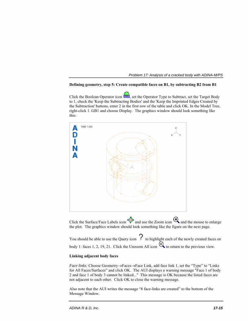
Defining geometry, step 5: Create compatible faces on B1, by subtracting B2 from B1

Click the Boolean Operator icon , set the Operator Type to Subtract, set the Target Body to 1, check the 'Keep the Subtracting Bodies' and the 'Keep the Imprinted Edges Created by the Subtraction' buttons, enter 2 in the first row of the table and click OK. In the Model Tree, right-click 1. GB1 and choose Display. The graphics window should look something like this:

TIME 1.000

X Y

Z

Click the Surface/Face Labels icon and use the Zoom icon and the mouse to enlarge the plot. The graphics window should look something like the figure on the next page.

You should be able to use the Query icon to highlight each of the newly created faces on

body 1: faces 1, 2, 19, 21. Click the Unzoom All icon to return to the previous view. Linking adjacent body faces Face links: Choose GeometryFacesFace Link, add face link 1, set the “Type” to “Links for All Faces/Surfaces” and click OK. The AUI displays a warning message "Face 1 of body 2 and face 1 of body 3 cannot be linked..." This message is OK because the listed faces are not adjacent to each other. Click OK to close the warning message. Also note that the AUI writes the message “8 face-links are created” to the bottom of the Message Window.


17-16 ADINA Primer

F1

F2

F3

F4

F5

F6

F7

F8

F9

F10

F11

F13

F14

F15

F17

F18

F19

F20

F21

F22

Labels for faces 1 and 19

Specifying the fixed boundaries In order to define the fixed boundaries, we need to know some of the face numbers on body 1. The following figure shows the faces that need to be fixed.

F17

F16

F18

F15

x y

z



Click the Apply Fixity icon , set the “Apply to” field to Face/Surface, enter the following information and click OK. Face/Surface Body #

15 1 16 1 17 1 18 1

Specifying the loads We constrain the faces upon which we apply the forces to points, then we apply the forces to the points. The following figure shows the faces and points:

Faces 11 and 12 are constrained to point 21.Faces 13 and 14 are constrained to point 22.

P21

P22

F13

F12

F14

F11

x y

z


17-18 ADINA Primer

Constraint equations:. Choose ModelConstraintsConstraint Equations, define the following constraint sets and click OK.

Constraint Set

Entity Type

Entity #

Body #

Slave DOF

Master Entity Type

Point # Master DOF

1 Face 11 1 Z-Trans Point 21 Z-Trans 2 Face 12 1 Z-Trans Point 21 Z-Trans 3 Face 13 1 Z-Trans Point 22 Z-Trans 4 Face 14 1 Z-Trans Point 22 Z-Trans

(we abbreviate Z-Translation by Z-Trans in this table)

Loads: Click the Apply Load icon , make sure that the Load Type is Force and click the Define... button to the right of the Load Number field. In the Define Concentrated Force dialog box, add force 1, set the Magnitude to 5E5, the Direction to (0, 0, 1) and click OK. In the Apply Load dialog box, make sure that the “Apply to” field is set to Point. In the first two rows of the table, set the Point # to 21 and 22 respectively, then click OK to close the dialog box.

When you click the Boundary Plot icon and the Load Plot icon , the graphics window should look something like this:

B

B

B

B

U1

U2

U3 1 2 3

B - - - - - -

TIME 1.000

X Y

Z

PRESCRIBEDFORCE

TIME 1.000

500000.



Defining the material

Click the Manage Materials icon and click the Elastic Isotropic button. In the Define Isotropic Linear Elastic Material dialog box, add material 1, set the Young’s Modulus to 2.07E5, the Poisson’s ratio to 0.29 and click OK. Click Close to close the Manage Material Definitions dialog box. Defining the element groups Although one element group could have been used in this model, we use two element groups instead , one element group for the crack bodies, and another element group for the rest of the model.

Element group definition: Click the Element Groups icon , add group number 1, set the Type to 3-D Solid and click Save. Then add group number 2, make sure that the Type is 3-D Solid and click OK. Subdividing the bodies We will specify a uniform element size in geometry body 1 and a smaller uniform element

size in the crack bodies (2 and 3). Click the Subdivide Bodies icon , make sure that the Body # is set to 1, set the Element Edge Length to 8 and click Save. Then set the Body # to 2, set the Element Edge Length to 3, enter 3 in the first row of the table and click OK. Meshing

First click the Hidden Surfaces Removed icon so that we don't see the dashed hidden lines in the mesh. Also in the Model Tree, right-click 7. WHOLE_MODEL and choose Display.

Click the Mesh Bodies icon , set the Element Group to 1 and set the Nodes per Element to 27. Now click the Advanced tab, set the “Int. Angle Deviation” to 40, “Even Subdivisions on” to “Every Edge on Linked Faces” and “Mid-Face Nodes” to “Mid-point on Diagonal of Quad Face”. Set the first two rows of the table to 2, 3 and click OK. You can ignore and close the Warning dialog box that appears. The graphics window should look something like the top figure on the next page.

Click the Mesh Bodies icon , make sure that the Element Group is set to 2 and set the Nodes per Element to 27. Now click the Advanced tab, set the “Int. Angle Deviation” to 40, “Even Subdivisions on” to “Every Edge on Linked Faces” and “Mid-Face Nodes” to “Mid-point on Diagonal of Quad Face”. Set the first row of the table to 1 and click OK. The graphics window should look something like the bottom figure on the next page.


17-20 ADINA Primer

B

U1

U2

U3 1 2 3

B - - - - - -

TIME 1.000

X Y

Z

PRESCRIBEDFORCE

TIME 1.000

500000.

C

B

B

B

B

B

C

C

B

B

B

BB

BB

BB

B

B

B

B

BB

B

B

B

C

C

C

C

CC

CC

C

C

CCC

B

BB

B

B

B

BB

B

B

B

C

CC

CC

B

B

BB

B

B

B

B

B

B

C

B

C

B

B

C

C

BB

C CC

CC

C

C

C

B

B

B

B

B

B

BB

C

C

BBB B

BBB

BBBB

BBB

BBBB

B

BBB B

BBB B

BBB

BBB

BBB

B

BB

BB

B

BBB

BBBBB

BB

CC

CCC

CCCC

CC

CCCC

CCCC

CCCC

CC

CC

C

CC

B

C

BB

C

U1

U2

U3 1 2 3

B CC - - - - - -

TIME 1.000

X Y

Z

PRESCRIBEDFORCE

TIME 1.000

500000.



Crack definition, step 1: Split the meshes on B2 and B3

In the Model Tree, right-click 2. EG1 and choose Display. Click the Boundary Plot icon

to hide the boundary conditions. Then use the Pick icon and the mouse to enlarge the mesh. The graphics window should look something like this:

TIME 1.000

X Y

Z

Now click the Shading icon , the Cull Front Faces icon and the No Mesh Lines icon

. The graphics window should look something like the top figure on the next page. No incompatibilities can be seen in the mesh. Now choose MeshingNodesSplit Mesh, set 'Split Interface Defined By' to 'Surfaces/Faces', make sure that 'At Boundary of Interface' is set to 'Split Only Nodes on External Boundary', enter the following information in the table and click OK. Face/Surface Body #

5 2 1 3

Now use the Pick icon and the mouse to rotate the mesh plot until the graphics window looks something like the bottom figure on the next page.


17-22 ADINA Primer

TIME 1.000

X Y

Z

TIME 1.000

X Y

Z

Faces with duplicate nodes are visible

The cracked faces (with duplicate nodes) are visible in the plot.



Crack definition, step 2: Create the CRACK-SVS definition Fracture control: Choose ModelFractureFracture Control, check the Fracture Analysis field, set the Dimension to 3-D Crack, set the Method to 'Virtual Crack Extension (SVS)' and click OK. CRACK-SVS definition: Choose ModelFracture3-D SVS Crack and add Crack Number 1. In the Crack Advance Stations box, set the 'Option' to 'Equally Spaced at Number of Locations' and set the 'Number of Crack Advance Stations' to 37. In the Radial Domains box, set the 'Maximum Outer Radius' to 5 and the 'Number of Domains' to 3. Set the 'Binormal Direction of Crack Front' to 'Down'. In the Closed Crack Front box, set 'Starts At' to 'Node Closest to Given Coordinate' and the Coordinate to (35, 0, 0). Then make sure that 'Side' is set to Top, enter 5, 2 in the first row of the table, then set 'Side' to Bottom, and enter 1, 3 in the first row of the table. Then click OK.

When you click the Redraw icon , the graphics window should look something like this:

TIME 1.000

X Y

Z

The symbol is plotted for each virtual shift. This symbol is interpreted as shown in the figure on the next page.


17-24 ADINA Primer

Position of crack advance stationon crack front

Domain radius

Direction ofvirtual shift,

directiona

There are 37 crack advance stations and three radial domains, for a total of 111 virtual shifts.

You can use the Query icon to click on each virtual shift symbol, to determine the crack advance station number, radial domain number and virtual shift number for the virtual shift. Generating the data file, running ADINA Structures, loading the porthole file

Click the Save icon and save the database to file prob17. Click the Data File/Solution

icon , set the file name to prob17, make sure that the Run Solution button is checked and click Save. When ADINA Structures is finished, close all open dialog boxes, set the Program Module drop-down list to Post-Processing (you can discard all changes), click the Open icon

and open porthole file prob17. Plotting the deformed mesh

We need to magnify the plotted displacements. Click the Scale Displacements icon . The displacement magnification factor appears to be too large for this model, so we will reduce it.

Click the Modify Mesh Plot icon and click the Model Depiction… button. Set the “Magnification Factor” to 40 and click OK twice to close both dialog boxes.

Now click the Shading icon . The graphics window should look something like the figure on the next page.



TIME 1.000 DISP MAG 40.00

X Y

Z

Determining the maximum displacement Choose ListExtreme ValuesZone, set Variable 1 to (Displacement:Z-DISPLACEMENT) and click Apply. The AUI reports that the maximum Z-displacement is 1.57003E-01 (mm) at node 12631 (your node number may be different, but the Z-displacement should be very close to ours). Click Close to close the dialog box. Plotting the element groups in different colors In the remaining mesh plots, we do not want to view the constraint equations. Choose DisplayGeometry/Mesh PlotDefine Style, set the Constraint Depiction to OFF and click

OK. Click the Clear icon , then the Mesh Plot icon . Notice that the constraint

equation lines are not displayed. Now click the Cut Surface icon , set the Type to Cutting Plane, the “Below the Cutplane” field to “Display as Usual”, the “Above the Cutplane” field to “Do not Display” and click OK.

Click the Color Element Groups icon . The graphics window should look something like the figure on the next page.


17-26 ADINA Primer

TIME 1.000

X Y

Z

Click the Color Element Groups icon to turn off the element group colors. Examining the meshing near the crack front line

Click the Clear icon , then the Mesh Plot icon . In the Model Tree, expand the Zone keyword, right click on 2. EG1 and choose Display. Let=s magnify the displacements so that we can see the crack opening under the load. Click

the Scale Displacements icon . The graphics window should look something like the top figure on the next page. Let's plot just the elements in element group 1 that are below the crack. Click the Split Zone

icon . In the Split Zone dialog box, click the ... button to the right of the 'With Cutting Plane' field. In the Define Cutsurface Depiction dialog box, set 'Defined by' to Z-Plane, the Coordinate Value to 0.01 and click OK. In the Split Zone dialog box, set 'Consider Only Elements in Zone' to EG1, set the field 'Place Elements Below Cutting Plane into Zone' to BELOW (you need to type this word, the case doesn't matter), and click OK. In the Model Tree, right click on 2. BELOW and choose Display. Then click the Node

Symbols icon and the Scale Displacements icon (to unscale the displacements). The graphics window should look something like the bottom figure on the next page.



TIME 1.000 DISP MAG 59.06

X Y

Z

TIME 1.000

X Y

Z

The thick blue line represents the crack front.


17-28 ADINA Primer

Now use the Zoom icon to zoom into the graphics window. The graphics window should look something like this:

Observe that the crack advance stations do not coincide with nodes. Also observe that the nodes are not shifted to the quarter-points near the crack front. Graphing the stress intensity factors The following diagram shows the crack front as viewed from above. The crack advance stations and the crack front coordinate are displayed.

Crack advance stations 1, 37

Crack advance station 2

Crack advance station 36

x

s�

y



Notice that crack advance stations 1 and 37 are at the same position. Clearly

(in degrees) 360length of crack front line

s

We can define a resultant that gives the angle for each virtual shift. Choose DefinitionsVariableResultant, add Resultant Name ANGLE_ON_CRACK_FRONT, define it as 360*<SVS_CRACK_FRONT_DISTANCE>/<SVS_CRACK_FRONT_LENGTH> and click OK. Now choose DefinitionsModel LineVirtual Shift, and add Model Line RADIAL_DOMAIN_1. Click the Auto... button, edit the table as follows and click Save (do not close the dialog box yet).

Virtual Shift # Crack # Radial Domain # Advance Station # Factor From 1 1 1 Step To 1 1 37 Now add Model Line RADIAL_DOMAIN_2, click the Auto... button, edit the table as follows and click Save (do not close the dialog box yet).

Virtual Shift # Crack # Radial Domain # Advance Station # Factor From 1 2 1 Step To 1 2 37 Finally add Model Line RADIAL_DOMAIN_3, click the Auto... button, edit the table as follows and click OK.

Virtual Shift # Crack # Radial Domain # Advance Station # Factor From 1 3 1 Step To 1 3 37


17-30 ADINA Primer

Now we graph the stress intensity factor IK along the crack front line. Click the Clear icon

, choose GraphResponse CurveModel Line), make sure that the Model Line Name is set to RADIAL_DOMAIN_1, set the X Coordinate to (User Defined: ANGLE_ON_CRACK_FRONT), the Y Coordinate to (Fracture: K-I) and click Apply. Set the Model Line Name to RADIAL_DOMAIN_2, the X Coordinate to (User Defined: ANGLE_ON_CRACK_FRONT), the Y Coordinate to (Fracture: K-I), the Plot Name to PREVIOUS and click Apply. Finally set the Model Line Name to RADIAL_DOMAIN_3, the X Coordinate to (User Defined: ANGLE_ON_CRACK_FRONT), the Y Coordinate to (Fracture: K-I), the Plot Name to PREVIOUS and click OK. The graphics window should look something like this:

0. 50. 100. 150. 200. 250. 300. 350. 400.9.

10.

11.

12.

13.

14.

15.

16.

*10

2

LINE GRAPH

Line RADIAL_DOMAIN_1



ANGLE_ON_CRACK_FRONT

K-I

The results change very little between radial domains 2 and 3. Choose GraphList and scroll to the bottom of the list. The value of K-I for angle

3.60000E+02 (degrees) should be around 1.59389E+03 MPa- mm . Your results might be slightly different due to free meshing. Let's repeat this procedure to determine the stress intensity factor IIIK along the crack front

line . Click the Clear icon , choose GraphResponse CurveModel Line), make sure that the Model Line Name is set to RADIAL_DOMAIN_1, set the X Coordinate to (User Defined: ANGLE_ON_CRACK_FRONT), the Y Coordinate to (Fracture: K-III) and click Apply. Set the Model Line Name to RADIAL_DOMAIN_2, the X Coordinate to (User Defined: ANGLE_ON_CRACK_FRONT), the Y Coordinate to (Fracture: K-III), the Plot



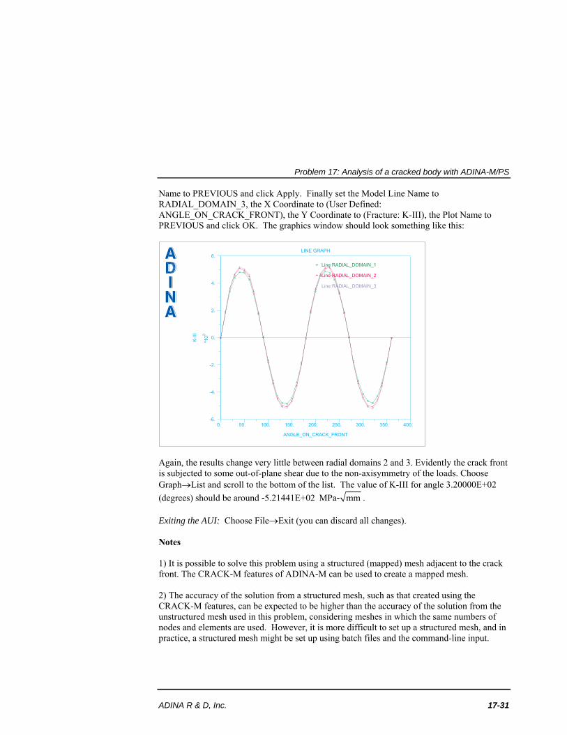
Name to PREVIOUS and click Apply. Finally set the Model Line Name to RADIAL_DOMAIN_3, the X Coordinate to (User Defined: ANGLE_ON_CRACK_FRONT), the Y Coordinate to (Fracture: K-III), the Plot Name to PREVIOUS and click OK. The graphics window should look something like this:

0. 50. 100. 150. 200. 250. 300. 350. 400.-6.

-4.

-2.

0.

2.

4.

6.

*10

2

LINE GRAPH




ANGLE_ON_CRACK_FRONT

K-I

II

Again, the results change very little between radial domains 2 and 3. Evidently the crack front is subjected to some out-of-plane shear due to the non-axisymmetry of the loads. Choose GraphList and scroll to the bottom of the list. The value of K-III for angle 3.20000E+02

(degrees) should be around -5.21441E+02 MPa- mm . Exiting the AUI: Choose FileExit (you can discard all changes). Notes 1) It is possible to solve this problem using a structured (mapped) mesh adjacent to the crack front. The CRACK-M features of ADINA-M can be used to create a mapped mesh. 2) The accuracy of the solution from a structured mesh, such as that created using the CRACK-M features, can be expected to be higher than the accuracy of the solution from the unstructured mesh used in this problem, considering meshes in which the same numbers of nodes and elements are used. However, it is more difficult to set up a structured mesh, and in practice, a structured mesh might be set up using batch files and the command-line input.


17-32 ADINA Primer

3) In the meshing for this problem, although 27-node hexahedral elements are specified in the input, a mixture of 27-node hexahedral elements and 10-node tetrahedral elements is generated. 4) For an unstructured mesh, shifting the nodes to the quarter-points can cause the elements to become overdistorted. Therefore the nodes are not shifted to the quarter-points in this CRACK-SVS definition. 5) The stress intensity factor IIK can also be graphed, but its value is negligible compared to

the other stress intensity factors.

problem description - adina description ... stations along the crack front. actual crack propagation...

Documents