HAL Id: tel-00817612https://tel.archives-ouvertes.fr/tel-00817612

Submitted on 25 Apr 2013

HAL is a multi-disciplinary open accessarchive for the deposit and dissemination of sci-entific research documents, whether they are pub-lished or not. The documents may come fromteaching and research institutions in France orabroad, or from public or private research centers.

L’archive ouverte pluridisciplinaire HAL, estdestinée au dépôt et à la diffusion de documentsscientifiques de niveau recherche, publiés ou non,émanant des établissements d’enseignement et derecherche français ou étrangers, des laboratoirespublics ou privés.

Probing the nuclear structure in the vicinity of 78Ni viabeta decay spectroscopy of 84Ga

Karolina Kolos

To cite this version:Karolina Kolos. Probing the nuclear structure in the vicinity of 78Ni via beta decay spectroscopyof 84Ga. Other [cond-mat.other]. Université Paris Sud - Paris XI, 2012. English. <NNT :2012PA112201>. <tel-00817612>

UNIVERSITE PARIS-SUD

ÉCOLE DOCTORALE : École Doctoral Particules, Noyaux, CosmosLaboratoire de Institut de Physique Nucléaire d'Orsay

DISCIPLINE Physique Nucléaire

THÈSE DE DOCTORAT

soutenue le 24/09/2012

par

Karolina KOLOS

Probing the nuclear structure in the vicinity of 78Ni

via beta decay spectroscopy of 84Ga

Directeur de thèse : Fadi IBRAHIM Directeur de Recherche, CNRS, IPN OrsayCo-directeur de thèse : David VERNEY Charge de Recherche, CNRS, IPN Orsay

Composition du jury :

Président du jury : Elias KHAN Professeur, Universite Paris SudRapporteurs : Bertram BLANK Directeur de Recherche,CNRS, CENBG Bordeaux

Volker WERNER Associate Professor, Yale UniversityExaminateurs : Jaen-Charles THOMAS Charge de Recherche,CNRS, GANIL

Fadi IBRAHIM Directeur de Recherche, CNRS, IPN OrsayDavid VERNEY Charge de Recherche, CNRS, IPN Orsay

Abstract

Thanks to advances in production of radioactive nuclear beams in the last two decades,we are able to study nuclear systems very far from stability. The region of the nu-clear landscape in the vicinity of 78Ni remains still unexplored. This region, with veryneutron-rich 78Ni hypothetically considered as a doubly magic core, is interesting interms of nuclear structures. The experimental information is equally important toguide the emerging shell-model effective interactions in this region. We have studiedβ-decay of a neutron rich 84Ga isotope at the ALTO facility in IPN Orsay (France).The fission fragments were produced with photo-fission reaction induced by 50 MeVelectron beam in a thick UCx target. For the first time the maximum electron driverbeam intensity at ALTO - 10µA - was used. The gallium atoms were selectively ionizedwith a newly developed laser ion source. With this ion source the ionization of thegallium was more than ten times higher compared to the surface ion source previouslyused by our group. The ions were separated with the PARRNe mass separator andimplanted on a movable mylar tape. Two germanium detectors in close geometry wereused for the detection of γ-rays and γ-γ coincidence measurement, and a plastic 4πβ

for beta tagging. We present the results of our experiment: the improved level schemesof the neutron-rich 83,84Ge and 84As isotopes. We discuss their structure and comparethe experimental results with the shell model calculations made with the new effectiveinteraction ni78− jj4b with 78Ni core, constructed in the framework of this thesis.

Keywords : ISOL technique, photofission. uranium carbide target, radioactivity, laserion source, magic numbers, shell model, nuclear structure.

Résumé

Grâce aux progrés de la production de faisceaux radioactifs au cours des deux dernièresdécennies, nous sommes à présent capables d’étudier les systèmes nucléaires très loinde la vallée de stabilité. La région de 78Ni, noyau encore inconnu supposé double-ment magique, reste encore inexplorée. Cette région est très intéressante en termesde structure nucléaire. En effet, les informations expérimentales obtenues sur l’espacede valence ouvert au dessus de 78Ni, nous permettront de construire des intéractionseffectives pour cette région. Nous avons étudié la désintégration de l’isotope 84Ga richeen neutrons auprès de l’installation ALTO à l’IPN d’Orsay. Les fragments de fissionont été produites par photo-fission induite par l’interaction d’un faisceau d’électron de50 MeV avec une cible épaisse de carbure d’uranium. Pour la première fois, ALTO aété utilisé dans ses conditions optimales, tant du point de vue de l’intensité du fais-ceau primaire (10µA d’électrons à 50 MeV) que de la méthode d’ionisation. En effet,les atomes de gallium ont été sélectivement ionisés à l’aide d’une source d’ions laser.Grâce à cette nouvelle source l’ionisation du gallium était plus de dix fois supérieurà celui de la source à ionisation de surface utilisée précédemment par notre groupe.Les ions séparés par le séparateur de masse PARRNe ont été implantés sur une bandede mylar mobile, entourée de deux détecteurs germanium placés en géométrie rap-prochés d’un détecteur plastique pour le marquage des désintégrations béta. Danscette thèse je présente les résultats de notre expérience obtenus pour les noyaux richesen neutrons 83,84Ge et 84As. Nous discuterons de leur structure et les compareronsaux résultats obtenus avec des calculs modèle en couches effectués avec la nouvelleinteraction ni78− jj4b construite dans le cadre de cette thèse.

Mot-clès : technique d’ISOL, photo-fission. carbure d’uranium, radioactivité, sourced’ionisation laser, numberes magiques, modèle en couches, structure nucléaire.

Remerciements

Tout d’abord, je remercie l’ancienne directrice de l’IPN Mme Dominique Guillemaud-Mueller et le nouveau directeur M. Faiçal Azaiez de m’avoir permis de mener ma thèsedans l’Institut de Physique Nucléaire.

Je souhaite remercier les membres de mon jury : mes deux rapporteurs Bertam Blanket Volker Werner pour leurs commentaires et questions et pour avoir apporteé leurcontribution à ce manuscrit avec attention et gentillesse, Elias Khan pour avoir ac-cepté la présidence et Jean-Charles Thomas pour l’étude scrupuleuse mon manuscritet aussi pour les discussions scientifiques.

Je tiens à remercier sincèrement mes deux directeurs de thèse : Fadi Ibrahim et DavidVerney. Je les remercie pour l’environnement exceptionel de travail qu’ils m’ont ap-porté grace à leur enthousiasme et leur bonne humeur. Je remercie Fadi pour laconfiance qu’il m’a accordée pendent ce travail de thèse et pour m’avoir guidée et ori-entée au moment des choix difficiles au cours de ma thèse. Merci également à Davidpour sa disponibilité, pour ses conseils très enchichissants, ses encouragements, pourla qualité de son encadrement scientifique et pour sa super lettre de recommendation :p

Je remercie Brigitte Roussière pour son encadrement pendent la premiére année dema thèse et de m’avoir donné l’opportinuté de participer à des mesures de radioactiv-ité de la cible de carbure d’uranium. Je voudrais remercier également à ChristopheLau pour le temps qu’il a consacré à examiner le partie de mon manuscrit concernantle travail sur la cible.

Je remercie le groupe NESTER dans son ensemble qui m’a accueilli. Merci à MegumiNiikura et Iulian Stefan pour leur conseils et nos discussions. Je voudrais remercieraux theésard : Benoit Tastet, Adrien Matta, Baptist Mouginot, Sandra Giron, DmitriTestov et Mathieu Ferraton (MERCI Mathieu!). Je ne peux pas oublier l’incroyableéquipe du Tandem-ALTO qui a permis le déroulement de l’expérience de cette theèse.L’équipe du laser: Franois LeBlanc, Serge Franchoo et Celine Bonnin pour le développe-ment d’une source d’ionisation laser. Merci à Sebastien Ancelin et Gauillame Mavillapour leur remarquable travail. Merci aussi à Kane vrai ami de travail qui m’a sauvéla vie plusieurs fois :)

Je veux aussi remercier chaleureusement Kamila Sieja et Fredèric Nowacki, experts duModèle en Couches, pour l’opportunité de travailler ensemble sur des intéractions effec-tives, nos discussions, leur disponibilité et pour notre excellent collaboration. Dziekuje,

że mnie “zaadoptowaliscie” :) oraz za wasze niesamowite wsparcie szczególnie w czasieostatnich miesiecy mojego doktoratu. Niezaprzeczalnie ogromna cześć mojego dok-toratu to Wasza zasługa!

Merci à ma famille : mojej Mamie, Tacie i siostrze za ich ogromne wsparcie w ciagutyh ostatnich kilku lat które spedziłam wiele kilometrów od nich. Ich miłość, dobrerady i optymizm które zawsze dodaja mi otuchy i siły. Chciałabym im podziékowaćza ich przeogromne zaufanie jakim mnie darza i poparcie w decyzjach jakie podej-muje nawet jeśli oznacza to troche wiécej kilometrów jakie nas dziela. Dziekuje mojejsiostrze Michasi za dojrzałość i wyrozumialość i za nasze wszystkie prześmiane roz-mowy telefoniczne. Dziekuje Danielowi za ogromne wsparcie w czasie mojej obrony,za jego obecność i pomoc w przygotowywaniach a w szczególności za opieke nad mojasiostra :)

Daavid, kiitos siitä, että saimme kasvaa yhdessä joka päivä. Kiitos jokaisesta yhdessävietetysthetkestä ja yhteisistä seikkailuista Ranskassa :) Kiitos kärsivällisyydestäsi kunolin kaikkein kärsimattömin, ymmärtäväisyydestäsi kun minulla oli vaikea päivä, kan-nustuksestasi, rakkaudestasi. Nämä kolme vuotta olivat sen arvoiset, koska vietin nesinun kanssasi.

Karolina

Contents

1 Introduction 11.1 Evolution of the N = 50 gap towards 78Ni . . . . . . . . . . . . . . . . 11.2 Evolution of collectivity in germanium isotopes (Z = 32) . . . . . . . 51.3 Single-particle energies in N = 51 isotonic chain . . . . . . . . . . . . . 7

2 Nuclear theory 112.1 Nuclear force . . . . . . . . . . . . . . . . . . . . . . . . . . . . . . . . 112.2 Shell model and residual interactions . . . . . . . . . . . . . . . . . . . 13

2.2.1 Independent particle model . . . . . . . . . . . . . . . . . . . . 132.3 Collectivity and deformations . . . . . . . . . . . . . . . . . . . . . . . 16

2.3.1 Rotational state in even atomic nuclei . . . . . . . . . . . . . . 172.3.2 4+

1 /2+1 ratio . . . . . . . . . . . . . . . . . . . . . . . . . . . . . 20

2.4 Reduced transition probabilities . . . . . . . . . . . . . . . . . . . . . . 20

3 Modern Shell Model Approach 233.1 Nuclear Shell Model . . . . . . . . . . . . . . . . . . . . . . . . . . . . 23

3.1.1 Structure of the effective interaction . . . . . . . . . . . . . . . . 253.1.2 The ANTOINE code . . . . . . . . . . . . . . . . . . . . . . . . 27

3.2 New effective interaction . . . . . . . . . . . . . . . . . . . . . . . . . . 28

4 Development of an experimental setup to characterize the release ofUCx target prototypes 354.1 Study of the feasibility of the experiment . . . . . . . . . . . . . . . . . 35

4.1.1 Simulation . . . . . . . . . . . . . . . . . . . . . . . . . . . . . . 384.1.2 The simulated spectrum and its interpretation . . . . . . . . . . 43

4.2 The experiment . . . . . . . . . . . . . . . . . . . . . . . . . . . . . . . 454.2.1 Description of the experiment . . . . . . . . . . . . . . . . . . . 454.2.2 Exploitation of the calculations and measured spectra . . . . . . 46

5 Production of radioactive ion beams 515.1 Production methods . . . . . . . . . . . . . . . . . . . . . . . . . . . . 515.2 Production of radioactive nuclei with fission reaction . . . . . . . . . . 53

5.2.1 Neutron-induced fission . . . . . . . . . . . . . . . . . . . . . . . 535.2.2 Photo-fission . . . . . . . . . . . . . . . . . . . . . . . . . . . . 54

5.3 Ion sources . . . . . . . . . . . . . . . . . . . . . . . . . . . . . . . . . . 575.4 The ALTO facility . . . . . . . . . . . . . . . . . . . . . . . . . . . . . 61

5.4.1 LINAC . . . . . . . . . . . . . . . . . . . . . . . . . . . . . . . . 62

5.4.2 Target and the ion source . . . . . . . . . . . . . . . . . . . . . 635.4.3 The laser ion source at ALTO . . . . . . . . . . . . . . . . . . . 645.4.4 Mass separator PARRNe . . . . . . . . . . . . . . . . . . . . . . 68

6 Experimental set-up 696.1 Experimental details . . . . . . . . . . . . . . . . . . . . . . . . . . . . 696.2 Detection system . . . . . . . . . . . . . . . . . . . . . . . . . . . . . . 70

6.2.1 The tape system . . . . . . . . . . . . . . . . . . . . . . . . . . 706.2.2 Electronics . . . . . . . . . . . . . . . . . . . . . . . . . . . . . . 726.2.3 Acquisition system . . . . . . . . . . . . . . . . . . . . . . . . . 74

6.3 Performance of the detection set-up . . . . . . . . . . . . . . . . . . . . 746.3.1 Germanium detectors . . . . . . . . . . . . . . . . . . . . . . . . 766.3.2 BGO shield . . . . . . . . . . . . . . . . . . . . . . . . . . . . . 786.3.3 Veto detector . . . . . . . . . . . . . . . . . . . . . . . . . . . . 81

7 Data analysis and results 837.1 Analysis procedure . . . . . . . . . . . . . . . . . . . . . . . . . . . . . 83

7.1.1 Time spectra . . . . . . . . . . . . . . . . . . . . . . . . . . . . 847.1.2 Determination of the half-life . . . . . . . . . . . . . . . . . . . 857.1.3 The γ-γ coincidences . . . . . . . . . . . . . . . . . . . . . . . . 88

7.2 Experimental results . . . . . . . . . . . . . . . . . . . . . . . . . . . . 907.2.1 The β-gated energy spectrum . . . . . . . . . . . . . . . . . . . 907.2.2 Results for 84Ge . . . . . . . . . . . . . . . . . . . . . . . . . . . 907.2.3 Results for 83Ge . . . . . . . . . . . . . . . . . . . . . . . . . . . 957.2.4 Results for 84As . . . . . . . . . . . . . . . . . . . . . . . . . . . 98

7.3 Spin assignment . . . . . . . . . . . . . . . . . . . . . . . . . . . . . . . 104

8 Discussion 1118.1 Nuclear structure of 84Ge . . . . . . . . . . . . . . . . . . . . . . . . . . 1118.2 Nuclear structure of 83Ge . . . . . . . . . . . . . . . . . . . . . . . . . . 125

9 Conclusions and outlook 1339.1 Conclusions . . . . . . . . . . . . . . . . . . . . . . . . . . . . . . . . . 1339.2 Outlook . . . . . . . . . . . . . . . . . . . . . . . . . . . . . . . . . . . 135

Bibliography 137

List of Figures

1.1 Chart of nuclei . . . . . . . . . . . . . . . . . . . . . . . . . . . . . . . 21.2 Experimental E(2+) and the ratios of 4+/2+ energies for Z = 30 − 38

and N = 46− 54 . . . . . . . . . . . . . . . . . . . . . . . . . . . . . . 31.3 Evolution of the N = 50 shell gap from the difference in the two

neutron binding energies between N = 50 , 52 isotones. . . . . . . . . 41.4 The excitation energies of the 5+, 6 + 7+ states with (νg9/2)−1(νd5/2)+1

configuration in the even-even N = 50 isotonic chain. . . . . . . . . . . 51.5 Systematics of the low-lying positive parity states of 72−84Ge. . . . . . . 61.6 Experimental B(E2) values for the Se, Ge and Zn isotopes. . . . . . . . 71.7 Systematics of the low-lying positive parity states in theN = 51 isotonic

chain. . . . . . . . . . . . . . . . . . . . . . . . . . . . . . . . . . . . . 8

2.1 The energy of the first 2+ excited state. . . . . . . . . . . . . . . . . . 132.2 The sequence of single-particle energies for the harmonic-oscillator po-

tential, with an additional orbit-orbit l2 term and with the spin-orbitterm. . . . . . . . . . . . . . . . . . . . . . . . . . . . . . . . . . . . . . 15

2.3 a) A potential surfaces for the first four multipole order distortions.b) A schematic illustration of the spherical and the two quadrupole-deformation shapes. c) A scheme of a vibrational motion. . . . . . . . . 18

2.4 Normal and anomalous levels of the triaxial rotor . . . . . . . . . . . . 192.5 The ratios of 4+

1 to 2+1 energies against N for the nuclei with N >= 30 20

3.1 Schematic view of the 78Ni core and the valence orbitals. . . . . . . . . 283.2 Calculated evolution of the N = 51 neutron effective single-particle

energies between 79Ni and 101Sn. . . . . . . . . . . . . . . . . . . . . . . 293.3 Schematic view of the wave function compositions in 87Kr and 89Sr. . . 303.4 Experimental E(2+) in the N = 50 isotonic chain compared with the

theoretical calculations . . . . . . . . . . . . . . . . . . . . . . . . . . . 303.5 The B(E2; 2+→ 0+) values in the N = 50 isotonic chain compared to

the shell model calculations . . . . . . . . . . . . . . . . . . . . . . . . 313.6 The experimental and calculated energy spectra for even-even N=50

isotones. . . . . . . . . . . . . . . . . . . . . . . . . . . . . . . . . . . . 323.7 The experimental and calculated energy spectra for even-odd N=50

isotones. . . . . . . . . . . . . . . . . . . . . . . . . . . . . . . . . . . . 333.8 The experimental and calculated energy spectra for even-even N=52

isotones. . . . . . . . . . . . . . . . . . . . . . . . . . . . . . . . . . . . 34

4.1 Decay chains . . . . . . . . . . . . . . . . . . . . . . . . . . . . . . . . 40

4.2 The simulated spectrum . . . . . . . . . . . . . . . . . . . . . . . . . . 444.3 Up: Scheme of steps for experimental procedure. Middle: a UCx pellet

in the oven. Bottom: germanium detector with pellet placed on thesupport system in front of the crystal . . . . . . . . . . . . . . . . . . . 47

4.4 Measurement spectrum of one of pellet prototypes . . . . . . . . . . . . 484.5 Comparison of the release fraction of krypton from pellets: COM30,

PARRNe and ARC-melting . . . . . . . . . . . . . . . . . . . . . . . . 49

5.1 (Left) Neutron production at 0 as a function of deuteron beam energy.(Right) Fission cross section of 238U as a function of neutron energy. . . 54

5.2 Distribution of fission fragments as a function of the excitation energyof 238U. . . . . . . . . . . . . . . . . . . . . . . . . . . . . . . . . . . . . 55

5.3 (a) (The solid lines (the left-hand scale) is the γ-quanta spectrum pro-duced by electrons with various energies (indicated in the figure). Theexperimental points (the right-hand scale) represent the 238U photo-fission cross section. (b) The fission yield per electron for 238U as afunction of electron energy. . . . . . . . . . . . . . . . . . . . . . . . . . 56

5.4 Schematic representation of surface ionization, resonant photo ioniza-tion and ionization by electron impact. . . . . . . . . . . . . . . . . . . 57

5.5 The evolution of the first ionization energy as a function of atomic number. 585.6 Drawing of the MK5 ion source. . . . . . . . . . . . . . . . . . . . . . . 595.7 Schematic of different methods of ionization and the corresponding cross

sections. . . . . . . . . . . . . . . . . . . . . . . . . . . . . . . . . . . . 605.8 The scheme of the ALTO facility. . . . . . . . . . . . . . . . . . . . . . 615.9 Time structure of the electron beam at the entrance of the accelerator. 625.10 Photo of the uranium carbide pellets . . . . . . . . . . . . . . . . . . . 635.11 The melting and boiling point . . . . . . . . . . . . . . . . . . . . . . . 645.12 Two step ionization scheme for gallium. . . . . . . . . . . . . . . . . . . 655.13 Schematic view of the laser ion source at ALTO . . . . . . . . . . . . . 665.14 Schematic view of the ionization source . . . . . . . . . . . . . . . . . . 675.15 Energy spectrum measured for mass 84 with surface ionization ion

source and wit the newly developed at ALTO laser ion source . . . . . 68

6.1 Schematic view of the tape station and the detection system . . . . . . 706.2 Simulation of the activity of 84Ga and its descendants on the tape during

the cycle of 4 s of “collection time“ and 1 s ”decay time“. . . . . . . . . 716.3 Schematic view of the electronic system. . . . . . . . . . . . . . . . . . 736.4 Top: Picture of the detection system. Bottom: Schematic view of the

detection system. . . . . . . . . . . . . . . . . . . . . . . . . . . . . . . 756.5 Efficiency of the germanium detectors measured with 152Eu, 137Cs and

60Co sources . . . . . . . . . . . . . . . . . . . . . . . . . . . . . . . . . 76

6.6 The precision plot of the energy calibration for GFOC24, GV1 germa-nium detectors. . . . . . . . . . . . . . . . . . . . . . . . . . . . . . . . 77

6.7 Resolution of the germanium detectors as a function of the energy. Theresolution is measured with the spectrum from 84Ga β-decay. . . . . . . 78

6.8 Pictures of the BGO crystals and the carbon cell. . . . . . . . . . . . . 796.9 Measured γ-ray spectrum of 60Co with and without Compton suppression 806.10 The suppression factor of the BGO shield as a function of incident γ-ray

energy . . . . . . . . . . . . . . . . . . . . . . . . . . . . . . . . . . . . 806.11 Picture of the Veto plastic detector . . . . . . . . . . . . . . . . . . . . 816.12 The β − γ coincidence spectra with background rejection. . . . . . . . . 82

7.1 Time distributions of β−γ coincidence events for the GFOC24 detector(upper) and the GV1 detector (lower plot). . . . . . . . . . . . . . . . . 85

7.2 Example of the determination of the half-life . . . . . . . . . . . . . . . 867.3 Procedure for the determination of the half-life. . . . . . . . . . . . . . 877.4 The γ-γ coincidence energy matrix . . . . . . . . . . . . . . . . . . . . 887.5 The coincidence spectra for line 624 keV. . . . . . . . . . . . . . . . . . 897.6 Single γ spectrum conditioned with β and BGO detectors. . . . . . . . 917.7 The results of the half-life determination for the lines of 84Ge. . . . . . 927.8 Single β gated energy spectrum zoomed to show the region of interest

(1370− 1400 keV) and the peak at 1389 keV . . . . . . . . . . . . . . . 937.9 The resulting level scheme of 84Ge . . . . . . . . . . . . . . . . . . . . . 947.10 The results of the half-life determination for the lines of 83Ge. . . . . . 957.11 Top: The coincidence spectra for line at 247 keV. Bottom: The coinci-

dence spectra for line at 1045 keV. . . . . . . . . . . . . . . . . . . . . . 977.12 The resulting level scheme of 83Ge . . . . . . . . . . . . . . . . . . . . . 987.13 The results of the half-life determination for the lines of 84As. . . . . . 997.14 The results of the half-life determination for the lines of 84As. . . . . . 1007.15 The coincidence spectra for γ-line at 42.7 keV, 100 keV and 242 keV. . 1017.16 The resulting level scheme of 84As. . . . . . . . . . . . . . . . . . . . . 1027.17 Intensity estimation as a function of time. . . . . . . . . . . . . . . . . 1057.18 Schematic picture of the determination of the Pn ratio from the mea-

sured intensities of γ-lines in 83,84As and known branching ratios. . . . . 1067.19 The final level scheme of the 83Ge, 84Ge isotopes with proposed spin

assignement. . . . . . . . . . . . . . . . . . . . . . . . . . . . . . . . . . 108

8.1 The systematics of the excitation energies in the N = 48 isotonic chain. 1128.2 The systematics of the excitation energies in the N = 52 isotonic chain. 1138.3 The experimental energy levels in N = 52 isotones compared with our

shell model calculation . . . . . . . . . . . . . . . . . . . . . . . . . . . 114

8.4 The experimental energies of 2+1 , 2

+2 and 4+

1 states for Z = 32 − 38

compared with theoretical calculation . . . . . . . . . . . . . . . . . . . 1158.5 The resulting level scheme of 84Ge in comparison in theoretical calcula-

tion. . . . . . . . . . . . . . . . . . . . . . . . . . . . . . . . . . . . . . 1158.6 The schematic view of the possible electric and magnetic mode transi-

tions assuming the 2+ spin for the third excited state. . . . . . . . . . . 1178.7 The pictorial comparison of the low lying energy states in 80Ge and 84Ge.1208.8 The schematic view of the possible electric and magnetic mode transi-

tions assuming 1+ and 2+ spin for the highest energy observed excitedstate. . . . . . . . . . . . . . . . . . . . . . . . . . . . . . . . . . . . . . 122

8.9 The experimental level scheme of 84Ge in comparison with low-spinstates obtained in theoretical calculation. . . . . . . . . . . . . . . . . 123

8.10 The experimental level scheme of 84Ge in comparison with with thetheoretical calculations . . . . . . . . . . . . . . . . . . . . . . . . . . 124

8.11 The systematics of the energy level of N = 51 even-odd nuclei comparedwith the shell model calculation . . . . . . . . . . . . . . . . . . . . . . 125

8.12 The resulting level scheme of 83Ge in comparison in theoretical calcula-tion. . . . . . . . . . . . . . . . . . . . . . . . . . . . . . . . . . . . . . 127

8.13 The schematic view of the possible electric and magnetic mode tran-sitions assuming the 1/2+ or 3/2+ spin for the third excited state in83Ge. . . . . . . . . . . . . . . . . . . . . . . . . . . . . . . . . . . . . . 128

8.14 The experimental level scheme of 83Ge in comparison with low-spinstates obtained in theoretical calculation. . . . . . . . . . . . . . . . . 131

8.15 Search for the core-coupled states in the experimental and theoreticallevel scheme of 83Ge . . . . . . . . . . . . . . . . . . . . . . . . . . . . 131

8.16 The composition of the wave functions to investigate the core-coupledstates . . . . . . . . . . . . . . . . . . . . . . . . . . . . . . . . . . . . 132

List of Tables

4.1 Radioactive nuclids used in the simulation . . . . . . . . . . . . . . . . 424.2 The γ -lines of the elements of interest identified in the spectrum . . . 43

7.1 The final list of γ-lines observed in the β-decay of 84Ga assigned to thede-excitation from the excited states of 84Ge. . . . . . . . . . . . . . . . 92

7.2 Contribution of the activities of rubidium isotopes in peaks at 1385 keVand 1389 keV. . . . . . . . . . . . . . . . . . . . . . . . . . . . . . . . . 93

7.3 The list of γ-lines observed in the β-decay of 84Ga belonging to theexcited states of 83Ge. . . . . . . . . . . . . . . . . . . . . . . . . . . . 96

7.4 The final list of γ-lines observed in the β-decay of 84Ga assigned to thede-excitation from the excited states of 84As. . . . . . . . . . . . . . . . 103

7.5 The intensities of the most intense four γ-lines in 84As relative to 247.7keV1067.6 The relative population, the logft values and the spin assignements of

the excitation levels in 84Ge. . . . . . . . . . . . . . . . . . . . . . . . . 1077.7 The relative population, the logft values and the spin assignements of

the excitation levels in 83Ge. . . . . . . . . . . . . . . . . . . . . . . . . 107

8.1 The experimental energies of excitation levels in 84Ge and proposedcalculated ones with the spin assignements and wave functions. . . . . . 116

8.2 The calculated reduced transition probabilities and the partial γ-raytransition probabilities for the assignement of the spin and parity of theexperimental level at 1389 keV. . . . . . . . . . . . . . . . . . . . . . . 118

8.3 Calculated spectroscopic quadrupole moments for the first two 2+ andone 3+states in 84Ge . . . . . . . . . . . . . . . . . . . . . . . . . . . . 119

8.4 The calculated reduced transition probabilities and the partial γ-raytransition probabilities for the assignement of the spin and parity of theexperimental level at 3502 keV. . . . . . . . . . . . . . . . . . . . . . . 122

8.5 Wave functions of the calculated ground state 0+ and the first 2+ excitedstate in 82Ge . . . . . . . . . . . . . . . . . . . . . . . . . . . . . . . . . 126

8.6 The experimental energies of excitation levels in 83Ge and proposedcalculated ones with the spin assignements and wave functions. . . . . . 126

8.7 The calculated reduced transition probabilities and the partial γ-raytransition probabilities for the assignement of the spin and parity of theexperimental level at 1045 keV. . . . . . . . . . . . . . . . . . . . . . . 129

8.8 The calculated reduced transition probabilities and the partial γ-raytransition probabilities for the assignement of the spin and parity of theexperimental level in 83Ge at 2026 keV . . . . . . . . . . . . . . . . . . 130

Chapter 1

Introduction

Contents1.1 Evolution of the N = 50 gap towards 78Ni . . . . . . . . . . . . 1

1.2 Evolution of collectivity in germanium isotopes (Z = 32) . . 5

1.3 Single-particle energies in N = 51 isotonic chain . . . . . . . . 7

1.1 Evolution of the N = 50 gap towards 78Ni

Recent advances in the production and purification of radioactive ion beams have madea region of nuclei near 78Ni more accessible for the experimental studies. The veryneutron-rich 78Ni (N/Z ' 1.8) is hypothetically considered as doubly magic nucleuswith 28 protons and 50 neutrons. It was synthesized and identified in-flight usingthe projectile fragmentation method [1] but its excitation modes remain unknown andrely on the extrapolation of the properties of its neighbors. The region around 78Ni isinteresting in terms of nuclear structures. Firstly, as this nucleus (in some scenarios)is one of the waiting-points in the r-process, testing the rigidity of its gaps remains ofa special interest. Secondly, the experimental information is important to guide theemerging shell-model effective interactions in this region. The knowledge of the singleparticle energies of 78Ni is crucial for shell model studies which utilize this nucleus asa core [2] and to validate the empirical universal monopole interactions [3, 4, 5].

From the evolution of the effective single-particle energy of the proton in Cu isotopesis was shown that the 1f5/2 orbital goes down and crosses the 2p3/2 orbital at N =

44 − 46 [6] when approaching the more neutron-rich region. It was interpreted asan indication of the reduction of the Z = 28 shell gap due to the tensor part of thenucleon-nucleon interaction [7, 4]. The magic number 50 originates from the spin-orbitpart of the nuclear interaction which lowers the energy of g9/2 orbit from the N = 4

major shell and locates it close to the orbits from N = 3 major shell. Its partner,the g7/2 orbit, is pushed to the upper edge of the gap, above/below the d5/2 orbit.The 78

28Ni50 isotope belongs to the same family as other doubly spin-orbit nuclei as206 C14, 42

14Si28 and 13250 Sn82. The latter has the major characteristics of a doubly-magic

7828Ni50

4214Si28

13250 Sn82

sd-pf : deformed

gds-hfp : magic

pf-gds : ?

d5/2

s1/2d3/2

8

14

20

f7/2

f5/228

p3/2p1/2g9/2

❳H.O.

❳H.O.

4214Si28

Figure 1.1: Left top: Schematic representation of the orbitals in 42Si. Right: Chart ofnuclei. The position of very neutron rich 42Si,78Ni and 132Sn is pointed on thechart.

spherical nucleus [8, 9] while the two others are deformed [10, 11]. The magic numbers14 and 28 are not a major harmonic oscillator closures but come from the additionalspin-orbit interaction (Figure 1.1). In 42Si, the first excited state was measured to beat low energy and explained as an indication of the existence of the erosion of boththe Z = 14 and N = 28 shell closures caused by action of the mutual proton andneutron forces and to the quadrupole correlations between states bounding the twogaps [10]. Such a deformed configuration could be found for the ground state of 78Nior a low-lying state [12].

The evolution of the size of the N = 50 shell gap between Z = 28 and Z = 38 de-pends on proton-neutron interactions between the proton πf5/2, πp3/2 orbitals and theneutron νg9/2 and νd5/2 orbitals [13]. The 2+ states in the N = 50 isotonic chainare expected to be formed by proton excitations within πfp shells. The experimen-tal energies of 2+ excited states and the ratios of the energies of 4+ to 2+ statesfor Z = 30 − 38 (N = 46 − 54) are plotted in Figure 1.2. The high energies of the2+ states (and low 4+/2+ ratio at N = 50) point to the persistence of the N = 50 gap .

Neutron number46 48 50 52 54

E(2

+)

[MeV

]

0

0.2

0.4

0.6

0.8

1

1.2

1.4

1.6

1.8

2

Sr

Kr

Se

Ge

Zn

Neutron number46 48 50 52 54

E(4

+)/

E(2

+)

0

0.5

1

1.5

2

2.5

3

3.5

4

Kr

Se

Ge

Zn

Figure 1.2: (Left:) Experimental E(2+) and (right:) the ratios of 4+/2+ energies for Z =

30− 38 and N = 46− 54.

The behavior of the two-nucleon separation energies is a widely used indicator ofstructural evolution as for the emergence of magic numbers. The gap derived fromthe difference of two-neutron binding energies (BE2n(N = 52) − BE2n(N = 50)) isplotted in Figure 1.3. It displays a staggering as a function of the parity of Z anda change of slope at Z = 32. Two-neutron separation energies provide evidence forthe reduction of the N = 50 shell gap energy towards germanium (Z = 32, whichwas not expected from the systematics of the 2+ energies or the B(E2) values) and asubsequent increase at gallium (Z = 31) which was interpreted by Hakala et al. [14]as an indication of the persistent rigidity of the shell gap towards nickel (Z = 28).The reduction of the spherical gap at Z = 32 was described by Bender et al. [15] interms of beyond mean-field dynamic collective quadrupole correlations, and confirmedwith the empirical evaluation of one or two-neutron separation energies of ground orisomeric state by Porquet et al. [12].

The size of a gap is related to the energy of the states arising from the 1p− 1h excita-tions across it. As the N = 50 shell gap is formed between the g9/2 and d5/2 orbits, thecorresponding 1p − 1h states have a (νg9/2)−1(νd5/2)+1 configuration. This gives riseto a multiplet of six states with spin values J ranging from 2 to 7. All the membersof this multiplet were successfully identified in 90

40Zr using the neutron pick-up reaction9040Zr(3He,α) [16] and in 88

38Sr using the neutron stripping reaction 8838Sr(d, p) [17]. The

high-spin states of 8636Kr and 84

34Se were studies via 82Se(7Li,p2n) reaction[18] and infusion fission reaction [19]. More recently, the excited states in 82

32Ge were studied byspontaneous fission of 248Cm and two states with spins 5+ and 6+ were proposed [20].The energies of the 5+, 6+ and 7+ states for N = 50 isotones as a function of protonnumber Z are drawn in Figure 1.4. Since the excitation energy is related to the size of

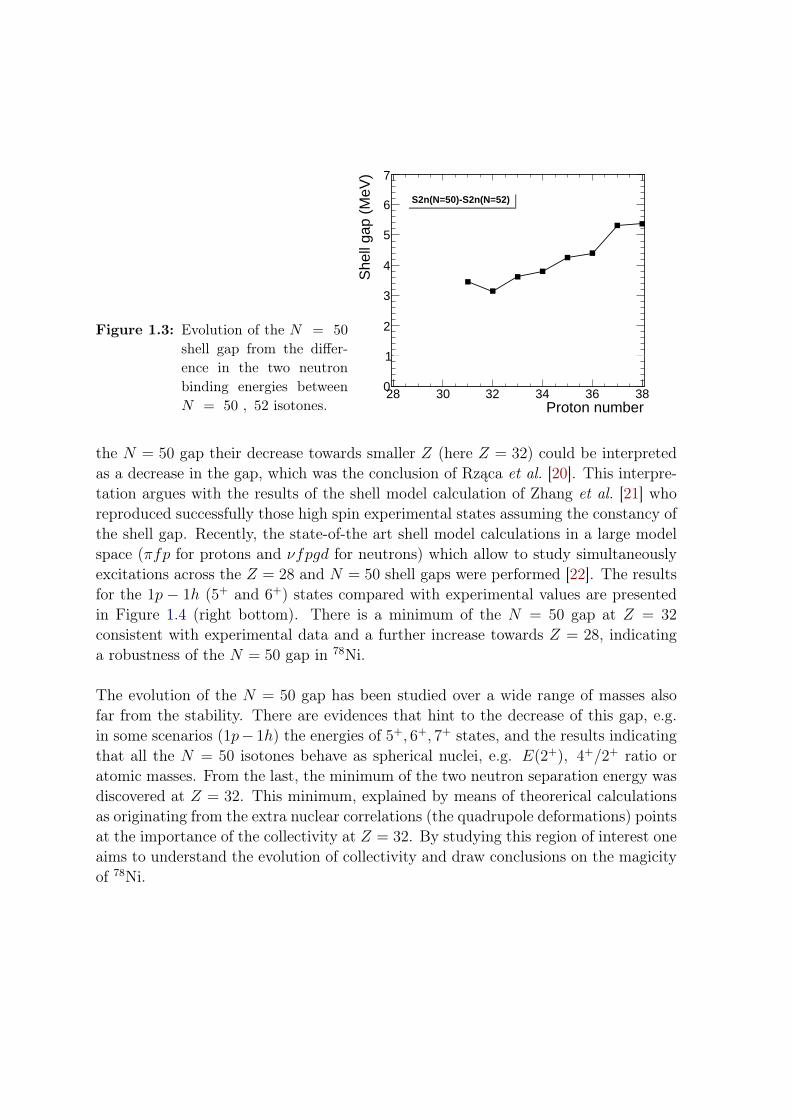
Figure 1.3: Evolution of the N = 50

shell gap from the differ-ence in the two neutronbinding energies betweenN = 50 , 52 isotones. Proton number

28 30 32 34 36 38

She

ll ga

p (M

eV)

0

1

2

3

4

5

6

7

S2n(N=50)-S2n(N=52)

the N = 50 gap their decrease towards smaller Z (here Z = 32) could be interpretedas a decrease in the gap, which was the conclusion of Rząca et al. [20]. This interpre-tation argues with the results of the shell model calculation of Zhang et al. [21] whoreproduced successfully those high spin experimental states assuming the constancy ofthe shell gap. Recently, the state-of-the art shell model calculations in a large modelspace (πfp for protons and νfpgd for neutrons) which allow to study simultaneouslyexcitations across the Z = 28 and N = 50 shell gaps were performed [22]. The resultsfor the 1p − 1h (5+ and 6+) states compared with experimental values are presentedin Figure 1.4 (right bottom). There is a minimum of the N = 50 gap at Z = 32

consistent with experimental data and a further increase towards Z = 28, indicatinga robustness of the N = 50 gap in 78Ni.

The evolution of the N = 50 gap has been studied over a wide range of masses alsofar from the stability. There are evidences that hint to the decrease of this gap, e.g.in some scenarios (1p− 1h) the energies of 5+, 6+, 7+ states, and the results indicatingthat all the N = 50 isotones behave as spherical nuclei, e.g. E(2+), 4+/2+ ratio oratomic masses. From the last, the minimum of the two neutron separation energy wasdiscovered at Z = 32. This minimum, explained by means of theorerical calculationsas originating from the extra nuclear correlations (the quadrupole deformations) pointsat the importance of the collectivity at Z = 32. By studying this region of interest oneaims to understand the evolution of collectivity and draw conclusions on the magicityof 78Ni.

Figure 1.4: The excitation energies of the 5+, 6 + 7+ states with (νg9/2)−1(νd5/2)

+1 con-figuration in the even-even N = 50 isotonic chain. Left: Experimental datafrom [16, 17, 18, 19, 20]. Right: Calculated values from [22] compared with theexperimental energies of the 5+ states.

1.2 Evolution of collectivity in germanium isotopes(Z = 32)

The intriguing features of the low-lying states in the even-even neutron-rich germa-nium isotopes have been discussed in a number of experimental and theoretical papers.The Ge isotopes around A ' 72 − 80 are well known to exhibit the shape coexis-tence phenomenon characterized by prolate-oblate and spherical-deformed competition[26, 27, 28, 29, 30, 24, 31]. The systematics of the low-lying positive parity states of72−84Ge is presented in Figure 1.5. In neutron-rich Ge isotopes (A = 72−80) neutronsoccupy the g9/2 orbit, which separates the N = 40 sub-shell gap and the N = 50 shellgap. This unique parity neutron orbit plays a distinctive role in the strength of theshell gap and in the development of collectivity in this mass region. Starting fromN = 40, the 2+ state in 72Ge isotope was measured to be lower as compared to 70Geat N = 38. The reduced transition probability was also measured higher indicating anincrease in collectivity around N = 40. This enhanced collectivity leads to a deformed

Neutron number40 42 44 46 48 50 52

Ene

rgy

(keV

)

0

500

1000

1500

2000

2500

3000

35002_1+2_2+4_1+4_2+ 6_1+0_2+3_1+

Figure 1.5: Systematics of the low-lying positive parity states of 72−84Ge.

ground state configuration in 72Ge which was found to be γ-soft [32]. The maximumof deformation is reached at N = 42 and then decreases with increasing number ofneutrons. Several experiments (two neutron transfer e.g. [33], Coulomb excitation[29]) were performed to study the structure of 74Ge. The first 0+,2+ and 4+ stateswere found to belong to the rotational ground-state band, the 0+

2 to be an intruderwhile the 2+

2 was interpreted as a band-head of the gamma vibration band [29]. The76−78Ge isotopes were also found to show the characteristics of an asymmetric rotorwith γ ∼ 30 [27]. The excitation levels in 80Ge located at N = 48 (with two holes inthe g9/2 orbit) were populated with β-decay of 80Ga by Hoff and Fogelberg [34], andrecently at ALTO [35, 36]. From the measurement of reduced transition probabilities[31] and comparison with the shell model calculations the 2+

1 and the 2+2 states in the

nucleus were shown to have different configurations. The structure of the semi-magic82Ge isotope (N = 50) was studied via β-decay of 82Ga [34, 37]. The 1p − 1h stateswith spins 5+, 6+ were identified with the spontaneous fission of 248Cm [20]. From therecent measurement of the reduced transition probabilities towards N = 50 a smoothdecrease in the B(2+

1 → 0+1 ) values (Figure 1.6) has been reported [24]. The slope of

the reduced transition probabilities is similar to the one in Se or Zn isotopes. The high(1348.17(12) keV) 2+ energy of 82Ge and low B(E2) value at the N = 50 indicate thepersistence of the magic 50 for germanium isotopes. When passing the neutron num-ber 50, the first attempt to study the 84Ge isotope was made at ISOLDE-CERN by

Neutron number40 42 44 46 48 50

B(E

2+->

0+)

(e2f

m4)

0

100

200

300

400

500

600

700

800

900

Se

Ge

Zn

Figure 1.6: Experimental B(E2)

values for the Se,Ge and Zn isotopes[23, 24, 25]. Asmooth decrease ofthe B(2+

1 → 0+1 )

values at N = 50 in-dicates a persistenceof the magic numberN = 50 (at Z =

30, 32).

Koster et al. [38] and at IPN Orsay by Lebois et al. [39]. The two γ-rays (624.3(7)keVand 1046.1(7)keV) were attributed as the de-excitation rays from the 2+

1 and 4+1 states.

Because of high 4+1 to 2+

1 energy ratio (R4/2 = E(4+1 )/E(2+

1 ) = 2.67) a sudden increaseof collectivity in 84Ge with two neutrons above N = 50 was proposed by Lebois. Thelocation of the 4+

1 state was not confirmed by Winger [37] who proposed the 4+1 state

at 1389.0(10)keV. This 4+1 state was not yet confirmed and more information is needed

on the excitation levels of this very neutron-rich isotope. It is extremely interestingto study how the nuclear collectivity evolves in this neutron-rich region while crossingthe magic number N = 50 and the rigidity of this magic number.

When following the systematics of the germanium isotopes in the N = 40− 50 regionone could expect to see a collective behavior in 84Ge. The nature of the collectivity canbe probed by measuring the excitation energies of the first 2+, 4+, 0+ excited states.In the experiment performed in the framework of this thesis we aimed to populate theexcited states in 84Ge via β-decay of 84Ga to study the evolution of the collectivity inthis neutron-rich nucleus beyond N = 50.

1.3 Single-particle energies in N = 51 isotonic chain

Systematics of the low-lying positive parity states in the N = 51 isotonic chain ispresented in Figure 1.7. The valence space that opens above 78Ni corresponds to theproton π(f5/2, p3/2, p1/2, g9/2) orbits and the neutron ν(g7/2, d5/2, d3/2, s1/2, h11/2) orbits.The spin of the ground-state of the N = 51 odd-even isotones from 81Zn up to 101Snare well established to be 5/2+ originating from the occupation by the valence neutronof the ν2d5/2 orbital [13, 40]. In the low-lying spectra of odd-even N = 51 isotonesstates correspond to the coupling of the ν2d5/2 neutron to the first 2+ excitation of thesemi-magic N = 50 core which gives rise to a multiplet of states with spins ranging

from 1/2+ to 9/2+. The second kind of states are the neutron quasi-particle states:1/2+, 3/2+, 7/2+ and at higher energy 11/2−, corresponding to the coupling of theN = 50 core 0+ ground state with the neutron. Those excited states are well identifiedin 89Sr (Z = 38, N = 51) and described in the framework of the core-particle couplingmodel [41, 42, 43]. An attempt to locate the neutron single-particle centroids by usingdirect (d, p) reaction with radioactive beams of 84Se and 82Ge has been made [44].The ν2d5/2 nature of ground state and the ν3s1/2 nature of the first excited state inboth 85Se and 83Ge were confirmed, but the results remained inconclusive for otherlow-lying states due to limited statistics.

SF=1.0SF=0.56

SF=0.9

SF=0.46

SF=0.35

SF=0.46

SF=0.9

SF=0.3

SF=0.49

SF=0.38SF=0.53

SF=0.52

2+ state of the even-even core

0

500

1000

1500

2000

2500

EHkeV

L

5ê2+ 5ê2+

1ê2+

H7ê2+L

5ê2+

1ê2+

H7ê2+L

H9ê2+L

H11ê2+L

H11ê2+LH13ê2+L

5ê2+

1ê2+

H7ê2+LH3,5ê2+L9ê2+

H9ê2+LH3,5ê2+LH3,5ê2+L11ê2+H1ê2+L7ê2+

5ê2+

1ê2+

H7ê2+L

5ê2+3ê2+9ê2+

3ê2+7ê2+

2+

2+

1ê2+

3081Zn51 32

83Ge51 3485Se51 36

87Kr51 3889Sr51

N=51

SF=0.32

Figure 1.7: Systematics of the low-lying positive parity states in the N = 51 isotonic chain.The spectroscopic factors “SF” from [44, 45, 46]

Due to the experimentally hard to reach region our knowledge on the low-lying states

in the N = 51 isotonic chain is poor. Up to now, 83Ge is the most exotic N = 51

isotone studied in terms of excitation energies but only few transitions were assigned toits level scheme. The low-lying excited states of 83Ge were populated in (d, p) reactionwith 82Ge beam at the Holifield Radioactive Ion Beam Facility (HRIBF) at Oak RidgeNational Laboratory (ORNL) [44, 47] and with the β-decay of 83Ga performed at IPNOrsay [48, 49] and at HRIBF [37] (β-decay of 83Ga, β − n decay of 84Ga). We studiedβ − n decay of 84Ga in order to populate yet unknown excited states of 83Ge. Theknowledge on the low-lying excited state in 83Ge would be extremely valuable in orderto perform a correct tuning of the monopole part of the residual interactions used inshell model to help us to understand the nuclear structures beyond N = 50.

N = 51 odd-odd 84As

From the β-decay study of 80−86As isotopes the ground state spin assignment (3−) wasproposed by Kratz et al. [50]. The first transitions in arsenic were identified first byOmtvedt et al. [51] who studied β-decay of 84−85Ge isotopes. The level scheme waslater updated by Winger et al. [52] and Lebois et al. [49]. The latest updated levelscheme of 84As was presented by Tastet [35]. He confirmed already known γ-transitionsat 42.7 keV, 100 keV, 242 keV, 386 keV and 608 keV [49, 51, 52], added two γ-lines,one at 346.5 keV the other at 794 keV, both in coincidence with 242 keV, and madean assignement of low-lying spins.

84As is the most exotic odd-odd N = 51 isotone of which a few excitation levelsand γ-transitions are identified. This nucleus is very interesting to study in terms ofproton-neutron interactions of the two valence particles. We populated the excitationlevels in 84As in the subsequent β-decay of 84Ge (originating from the decay of 84Ga).

Structure of thesis

In Chapter 2 a brief description of the current understanding of nuclear structure bymeans of various nuclear models with an accent on the shell model is described. Thereader can find the details of the structure of the shell model effective interactionsin Chapter 3 where we also present the result of work on the new shell model inter-action ni78 − jj4b. Chapter 4 is dedicated to the experimental study of the releaseproperties of different uranium carbide targets. This study was performed at IPNOrsay a priori to the β-decay study described later in this work. The ALTO facilityand the experimental approach to study β-decay of 84Ga are described in Chapter 5.The experimental details and the detection system are presented in Chapter 6. Inthe following Chapter 7 the procedure of data analysis is detailed and the results are

presented. In Chapter 8 the experimental results are compared with the shell modelcalculations. We discuss the structure of the exotic neutron-rich 83,84Ge. In the lastChapter 9 the conclusions and future perspectives are listed.

.

Chapter 2

Nuclear theory

Contents2.1 Nuclear force . . . . . . . . . . . . . . . . . . . . . . . . . . . . . 11

2.2 Shell model and residual interactions . . . . . . . . . . . . . . . 13

2.2.1 Independent particle model . . . . . . . . . . . . . . . . . . . . . 13

2.3 Collectivity and deformations . . . . . . . . . . . . . . . . . . . 16

2.3.1 Rotational state in even atomic nuclei . . . . . . . . . . . . . . . 17

2.3.2 4+1 /2

+1 ratio . . . . . . . . . . . . . . . . . . . . . . . . . . . . . . 20

2.4 Reduced transition probabilities . . . . . . . . . . . . . . . . . 20

2.1 Nuclear force

Nuclei are formed by composition of neutrons and positively charged protons. Thereis a repulsive Coulomb force between protons, therefore, in order for nuclei to exist,one can deduce immediately that there must be a strong attractive interaction thatcan overcome that repulsion and binds nucleons together. This interaction is calledthe strong interaction and has following properties [53]:

• At distances larger than 0.7 fm the force becomes attractive between spin-alignednucleons, becoming maximal at a center-center distance of about 0.9 fm. Beyondthis distance the force drops exponentially, until about 2.0 fm (beyond 2 to 2.5 fmCoulomb repulsion becomes the only significant force between protons). At thatdistance the nuclear force is negligibly feeble.

• At short distances it is stronger than the Coulomb force. Although predomi-nantly attractive, it becomes repulsive at nucleon separation of less than ∼ 0.7 fmbetween their centers. It keeps the nucleons at a certain average separation, evenif they are of different types. It is to be understood in terms of the Pauli exclu-sion force for identical nucleons (such as two neutrons or two protons), and alsoa Pauli exclusion between quarks of the same type within nucleons, when thenucleons are different (proton and neutron).

• It has a noncentral (a tensor) component (which does not conserve the orbitalangular momentum).

• It depends on whether the spins of the nucleons are parallel or antiparallel (nu-cleons as fermions have an intrinsic spin of 1/2~).

• It is nearly independent of whether the nucleons are neutrons or protons (charge-independence). Taking into account the correction for a repulsive Coulomb in-teraction between charged protons it implies that proton-proton and neutron-neutron interactions must have the same strength.

• There is only one bound state of the deuteron, a system with one proton and oneneutron, with the angular momentum J = 1 (parallel spins) and the total isospincoupling T = 0 suggesting that this proton-neutron interaction is the strongest.

The first nuclear model (called liquid-dropmodel) was first proposed by George Gamowin 1928 [54, 55] and later developed by Niels Bohr and John Wheeler [56, 57]. Theliquid-drop model was based on the assumption that a nucleus can be described asan incompressible, charged liquid-drop with volume proportional to the number ofnucleons A. According to this model, the nucleons move around at random and bumpinto each other frequently in the nuclear interior. Their mean free path is substantiallyless than the nuclear radius. The binding energy that keeps nucleons together isexpressed by the semi-emphirical Bethe-Weizsäcker mass formula [58]:

B(Z,A) = avA− asA2/3 − aCZ(Z − 1)A−1/3 − aA(A− 2A)2/A± δapA−1/2 (2.1)

where is av a volume, as a surface, aC Coulomb repulsion, aA asymmetry and appairing constant (they have following values: av = 15.85 MeV, as = 18.34 MeV,aC = 0.71 MeV, aA = 23.21 MeV and ap = 12 MeV). For most nuclei the binding en-ergy is about 8 MeV, however, there are exceptions at certain numbers of protons andneutrons, called magic numbers N/Z = 2, 8, 20, 40, 50, 82, 126. Although the liquid-drop model permits to correlate many facts about nuclear masses and binding energiesit does not give an explanation for the higher value of the nuclear binding energy ofmagic nuclei.

The importance of the magic numbers can be illustrated with the single-particle sepa-ration energy, which is defined as an energy required to remove one proton or neutronfrom the nucleus. The neutron/proton separation energy for doubly magic nuclei islargest (similarly to electrons in nobel gases) implying that paired neutrons/protonsresult in larger total binding per nucleon. Another proof of this shell effect can beillustrated by the evolution of the energy of the first excited 2+ states in the even-even nuclei. Figure 2.1 highlights the enormous differences in the energy of the 2+

excited states of magic nuclei in comparison with the non-magic ones. The same trend

is represented by the transition probabilities B(E2) which are correlated with the en-ergy of the first 2+ excited states. The occurrence of the magic numbers, from theexperimental point of view, was one of the strongest motivations for the formation ofthe nuclear shell model.

Figure 2.1: The energy of the first 2+ excited state [23].

2.2 Shell model and residual interactions

The nuclear shell model is based on an assumption that nucleons move in orbitalsclustered into shells (in analogy with electron shells in atom). The nucleons (protonor neutron) are characterized by their intrinsic spin and isospin. As fermions they aresubject to the Pauli principle which excludes two fermions being in the same state atthe same time. [53]

2.2.1 Independent particle model

In the simplest approach, the independent particle model, each nucleon is consideredas a quasi-independent particle moving in a certain spherically symmetric potentialU(r) produced by all the other nucleons. This central potential depends only on theradial distance from the origin to a given point. Then, the angular dependence of a

particle wave function Ψ is independent of the detailed radial behavior of the centralpotential. The Schrödinger equation for such a potential can be written as:

HΨ =

(p2

2m+ U(r)

)Ψnlm(r) = EnlmΨnlm , (2.2)

where U → 0 as r → 0. This equation is separable into radial, R(r), and angular,Y (θφ), part:

Ψnlm(r) = Ψnlm(rθφ) =1

rRnl(r)Ynl(θφ) . (2.3)

Here, n is the radial quantum number, l the orbital angular momentum quantumnumber and m is the eigenvalue of z-component of the orbital angular momentum, lz.For a given l, m has the values l, i− 1, l− 2, . . . , 0,−1,−2, . . . ,−(l− 1),−l. Since thenuclear potential is spherically symmetric, l is a good quantum number and each levelhas a degeneracy of 2(2l+1)1. The number of levels with certain l values is representedby n. There is a centrifugal force associated with each angular momentum L whichgenerates an additional centrifugal part of the nuclear potential:

Ucent =

∫Fcentdr =

∫L2

mr3dr = −~2l(l + 1)

2mr2. (2.4)

Then the radial Schrödinger equation becomes:

~2

2m

d2Rnl(r)

dr2+

[Enl − U(r)− ~2

2m

l(l + 1)

r2

]Rnl(r) = 0 . (2.5)

In the first approximation this central potential can be written as a harmonic oscillatorpotential

U(r) =1

2mω2r2 . (2.6)

The eigenvalues are Enl = (2n + l − 12)~ω. The energy levels fall into degenerate

multiplets defined by 2n+ 1 and a given multiplet contains more than one value of theprinciple quantum number n and of the orbital angular momentum l. These groupingsof degenerate levels appear as a result of the interplay of the harmonic-oscillator andcentrifugal potentials. Each energy level has 2(2l + 1) degenerate m states and, bythe Pauli principle, each nl level can contain 2(2l + 1) particles. The central partof the nuclear potential should have a rather uniform distribution in the interior ofthe nucleus due to an obvious saturation of the nuclear force. It is possible to otainby adding an attractive term l2 to the harmonic oscillator potential. The effects ofthis term increase with the orbital angular momentum of the particle. A strongerattractive interaction between high angular momentum particles lowers their energies.

1(2l+ 1) arises from the m degeneracy as there is (2l+ 1) values of m, the factor of 2 comes fromthe degeneracy of the intrinsic spin which has two possible values.

Those particles, because of the centrifugal force, spend a larger fraction of their timeat larger radii. Therefore, the addition of the l2 term is equivalent to a more attractivepotential at larger radii and comes closer to the desired effect of a more constantinterior potential. The consequence of adding the l2 term to the harmonic oscillatorpotential on the single particle level is illustrated in the middle panel of Figure 2.2.The degeneracy of the harmonic oscillator levels is broken as high angular momentumlevels are brought down in energy.

H.O. l2 ~l · ~s

Figure 2.2: The sequence of single-particle energies for the harmonic-oscillator potential,with an additional orbit-orbit l2 term and with the spin-orbit term [59].

However, it was an empirical modification to the harmonic oscillator potential (an in-troduction of a spin-orbit interaction term) by Göppert-Mayer [60], and independently,by Haxel [61], Jensen, and Suess, that enabled to reproduce the empirical magic num-bers. As protons and neutrons have an intrinsic spin 1/2, the total angular momentumof a nucleon in any orbit is given by the vector coupling of the orbital angular mo-mentum l with a spin angular momentum s = 1/2. The force felt by a given particlediffers according to whether its spin and orbital angular momenta are aligned parallelor antiparallel. In case of the parallel alignment the spin-orbit terms affects more

higher l values. The spin-orbit term can be written as Ul·s = −Uls 1r∂U(r)∂r

l · s, whereU(r) is a central potential and Uls is a strength constant. Finally, the potential hasform:

U(r) =1

2mω2r2 + Cl × l2 − CSO × l · s , (2.7)

where Cl and CSO are the angular momentum and spin-orbit coupling constants, re-spectively. The effects of this potential on the energy splittings are illustrated on thefar right in Figure 2.2. The spin-orbit potential can bring down the energy of thej = l + 1/2 orbit among the levels of the next lower shell what allows to reproducethe magic numbers. At the same time, it causes that each shell contains a majority oflevels of one parity, called normal-parity orbits, and one level of the opposite parity,called unique-parity (intruders) orbits. The unique-parity orbits are situated quite faraway from its original multiplets. In case of configuration mixing between differentlevels, the levels of different parity cannot be mixed (neglecting the very weak parity-nonconserving part of the weak interaction). This is why the unique-parity orbitsprovide an ideal testing ground for various nuclear models.

For double magic nuclei the sum of all magnetic substates m is coupled to zero, theground state of any doubly-magic nucleus is always 0+ (its total wave function isspherically symmetric with no preferred direction in space). In case of nuclei with oneparticle/hole outside/inside a closed shell, the spin and parity of the ground state isdetermined by the last filled particle/hole. The independent particle model is how-ever applicable in principle only to nuclei with a single nucleon outside a closed shell.To extend the applicability of the theoretical model one has to refer to nuclei withmore than one valence nucleon and that includes residual interactions between thesenucleons and allows for the breaking of closed shells.

2.3 Collectivity and deformations

The further from the closed shell and the more valence protons and neutrons areadded, the more collective motions appear. It causes a nucleus to collectively vibrate orrotate. Many nuclei, in the midshell, undergo permanent deformations (the quadrupoledeformation) even in the ground states. This deviation of the nuclear surface radiusfrom an average value R0 of the spherical nucleus of the same volume is parameterizedby expressing the nuclear radius in the direction Ω = (θ, φ):

R = R0 +∞∑λ=1

λ∑µ=−λ

αλµYλµ(θ, φ) , (2.8)

where Yλµ are spherical harmonics and αµ are deformation parameters. The constantterm λ = 0 is incorporated in R0. The dipole term (λ = 1), corresponding to a geomet-rical shift in the center of mass of the nucleus, gives rise to giant dipole resonances from

an oscillation of protons relative to neutrons in the nucleus at considerable energies(8 to 20 MeV). The lowest applicable shape component is the quadrupole deformation(λ = 2). The corresponding spherical harmonic amplitudes can be expressed in termsof Euler angles and two intrinsic variables α and β:

α21 = α2−1 = 0, α20 = β cos γ, α22 = α2−2 = β sin γ , (2.9)

where β represents the extent of the quadrupole deformation and γ gives the degreeof axial asymmetry. The relation between β, γ and the nuclear radius can be seenby representing the quadrupole shape in Cartesian coordinate system with the Z axischosen as a symmetry axis. Then, β = 0 represents spherical shape, β > 0 (γ = 0)prolate deformation (an expansion in one and compression in two directions, Ameri-can baseball) and β < 0 (γ = 60, 180) oblate deformation (an expansion in two andcompression in one directions, a disc), see Figure 2.3. Intermediate values of γ, forinstance 30, correspond to axially asymmetric shapes (in one of the two directionsperpendicular to the symmetry axis).

Due to the deformations there is a non-spherical distribution of nuclear matter of thenucleus which leads to a non-sphericity in the distribution of the overall electric chargeof the protons. Thus, the deformed nucleus has the electric quadrupole moment [53]:

Q0 =3

5πZR2

0β(1 + 0.16β) , (2.10)

where Q0 is the intrinsic quadrupole moment that would only be observed in the frameof reference in which the nucleus was at rest.

2.3.1 Rotational state in even atomic nuclei

The best known model of fixed asymmetry (triaxiallity) is Davydov and Filippovmodel [62]. The assignment of nuclear excited state to the so-called γ-vibrations isbased on the spin values of these levels and on the large probability of electromagnetictransitions which confirm the collective nature of the levels. Those rotational statesdo not entail changes of the internal state of the nucleus. The violation of the axialsymmetry of the even nuclei only slightly affects the rotational spectrum of the axialnucleus and some new rotational states appear. As the deviations from axial symmetryincrease some of those levels become much lower in energy (Figure 2.4). In practicalapplications of the Davydov model, one can extract the values of γ from the energyratio E2+2

/E2+1. It can be calculated for any γ from the expression:

E2+2

E2+1

=1 +X

1−X , (2.11)

Figure 2.3: a) A potential surfaces for the first four multipole order distortions. b) Aschematic illustration of the spherical and the two quadrupole-deformationshapes. c) A scheme of a vibrational motion.

where X =√

1− 89

sin2(3γ). Thus, E2+2/E2+1

→ ∞ for γ → 0 and E2+2/E2+1

→ 2 forγ → 30 (as seen in Figure 2.4).

Measurements of the transition probabilities between electric states in nucleus yieldimportant information on the nature of the excited states. One can study the prob-ability of the transition from the second excited 2+

2 state to the ground state and tothe first excited 2+

1 state. The first 2+1 state is referred to as a one-photon state while

the second 2+2 state is the two-phonon vibration of the nuclear surface. In this case

the transition from the second 2+1 state to the ground state takes place if the violation

of the oscillator approximation occurs. Assuming that one can assign two 2+ statesas the rotational levels, the value of γ can be obtained from the ratio of the transitionprobabilities [62, 53]

B(E2; 2+γ → 2+

y )

B(E2; 2+γ → 0+

y )=

107

(sin2(3γ)

9X2

)12

[1− 3−2 sin2(3γ)

3X

] . (2.12)

Figure 2.4: Normal and anomalous lev-els of the triaxial rotor. Forγ = 0 the energy spec-trum is identical to thatof an axially-symmetric nu-cleus. The violation of theaxial symmetry of the evennuclei leads to the appear-ance of some new energylevels (2+

2 , 3+1 , 4

+2 ). One

can obtain the value of γfrom the ratio of energiesE2+2

/E2+1[62].

The rotational energy of the nuclei or the transition probability between rotationalstates do not give us the information whether the nucleus is an elongated or oblateellipsoid. This information can be obtained from the electric moments in stationarystates (J,M = J), the so-called spectroscopic quadrupole moments:

Qspec = Q0

(3K2 − J(J + 1)

(J + 1)(2J + 3)

), (2.13)

here Q0 represents the intrinsic quadrupole moment. K is the projection of the totalangular momentum J along the z axis (symmetry axis). The most common distortionof spherical nuclei is quadrupole in nature. Therefore, the most common low-lyingvibrational excitations in deformed nuclei are quadrupole vibrations. They carry twounits of angular momentum and can be of two types with K = 0 and K = 2. Theformer are known as β vibrations, when K = 0 the vibration is aligned along thesymmetry axis and therefore preserves axial symmetry. The latter, with K = 2,is called γ vibration and represents a dynamic time dependent excursion from axialsymmetry. In even nuclei the mean values of the spectroscopic quadrupole momentin the ground state are equal to zero. A state of zero angular momentum can haveno preferred direction of the time averaged distribution in space and therefore noquadrupole moment. In the first and the second excited state of spin 2 the mean valueof the quadrupole moment has an opposite sign

Qspec22= −Qspec21

. (2.14)

2.3.2 4+1 /2+1 ratio

The ratio of 4+1 /2

+1 energies (Figure 2.5) can bring some structural signatures and its

absolute value is directly meaningful, especially in the region of heavy nuclei. Theratio can be devided into three parts: below 2.0 near magic nuclei, between 2.0 and2.4 slightly further away from magic numbers and values very close to 3.33 in midshellregions corresponding to rotational motion.

Figure 2.5: The ratios of 4+1 to 2+

1 energies against N for the nuclei with N ≤ 180. [53]

2.4 Reduced transition probabilities

In the β-decay of nuclei, a given initial nuclear state AXZi is converted into the groundstate or an excited state of the final nucleus AXZf , where Zf = Zi + 1. The transitionrate for nuclear beta decay is determined by the Qβ value (or energy release) and thestructure of the initial and final nuclear states. Beta decays with the fastest rates occurwhen the leptons carry away l = 0 angular momentum and are referred to as allowedtransitions. Decays with l > 0 are referred to as forbidden transitions. After the β-decay the final nucleus in an excited state can emit part or all of its excitation energyby electromagnetic radiation. These electromagnetic transitions are classified in terms

of multipole orders of electric and magnetic fields. The electromagnetic transitionbetween them can take place only if the emitted γ-ray carries away an amount ofangular momentum ~l such that ~Jf = ~Ji + ~l which means that |Ji − Jf | ≤ l ≤ Ji + Jfwhere J = ~J . Since the photon has an intrinsic spin of one, transitions with l = 0 areforbidden, and hence gamma transitions with Ji = 0 → Jf = 0 are not allowed. Aspecific l value determines the multipolarity of the gamma radiation: l = 1 is calleddipole, l = 2 is called quadrupole, etc.. In addition, when states can be labeled witha defined parity πi = ±1 and πf = ±1, the transitions between them are restrictedto the electric type of radiation when πiπf (−1)l is even and the magnetic type ofradiation when πiπf (−1)l is odd. The lowest allowed multipolarity in the decay ratedominates over the next higher one (when more than one is allowed) by several ordersof magnitude. The most common types of transitions are electric dipole (E1), magneticdipole (M1), and electric quadrupole (E2). Electromagnetic transition rates provideone of the most unambiguous tests for models of nuclear structure. The interactionof the electromagnetic field with the nucleons can be expressed in terms of a sum ofelectric, O(Eλ), and magnetic, O(Mλ), multipole operators with tensor rank λ [63]:

O =∑λµ

[O(Eλ)µ +O(Mλ)µ] (2.15)

For a given E or M operator of rank λ the electromagnetic transition rate WMi,Mf ,µ

(the probability for absorption or emission of a photon by a nucleus) can be expressedin terms of the matrix elements of the corresponding multipole operator as

WMi,Mf ,µ =

(8π(λ+ 1)

λ[(2λ+ 1)!!]2

)(k2λ+1

~

)|〈JfMf |O(λ)µ|JiMi〉|2 , (2.16)

where k is the wave-number for the electromagnetic transition of energy Eγ given byk = Eγ/~c = Eγ/(197 MeVfm) . The total rate for a specific set of states and a givenoperator is obtained by averaging over the Mi states and summing over Mf and µ:

Wi,f,λ =1

(2Ji + 1)

∑Mi,Mf ,µ

WMi,Mf ,µ =

(8π(λ+ 1)

λ[(2λ+ 1)!!]2

)(k2λ+1

~

) |〈Jf ||O(λ)||Ji〉|2(2Ji + 1)

.

(2.17)The last factor in this equation is referred to as a reduced transition probability B:

B =|〈Jf ||O(λ)||Ji〉|2

(2Ji + 1). (2.18)

It depends upon the direction of the transition. For electromagnetic transitions theinitial state is the higher-energy state. But in Coulomb excitation the initial state isthe lower-energy state (let us denote it Ja) while the final state is the higher-energystate (Jb). From the transition from lower to higher state one often uses the notation

B(↑). Then the value used for the electromagnetic transitions is B(b → a) = (2Ja +

1)/(2Jb + 1)B(↑ a→ b) . As an example, in case of an E2 transition between groundstate 0+

gs and the first excited state 2+1 , one obtains B(0+

gs → 2+1 ) = 5 ·B(↑ 2+

1 → 0+gs).

Often not only one transition from the initial to the final state is possible and weneed to consider mixed transitions of the form (E1 and M1) or (M1 and E2), etc..Each transition is characterized by its partial mean lifetime (τMλ, τEλ). The relationbetween the mean lifetime of the transition and the reduced transition probability forthe first two orders of magnetic transitions can be expressed as:

B(M1) =56.8

E3γτM1

µ2N MeV3 fs , (2.19)

B(M2) =74.1

E5γτM2

µ2N fm2 MeV5 ns . (2.20)

The values of the magnetic matrix elements are usually taken to be in units µN fmλ−1,where µN = e~/(2mpc) = 0.105 e fm is the nuclear magneton and mp is the mass ofthe proton. For the electric transitions:

B(E1) =0.629

E3γτE1

e2 fm2 MeV3 fs , (2.21)

B(E2) =816

E5γτE2

e2 fm4 MeV5 ps . (2.22)

A mean lifetime corresponds to the transition probability of the decaying state, therelation is given by τωλ = 1/Pi→f where (ω = M or E) [64]. The partial γ-raytransition probability Pi→f can be obtained from

Pi→f =

∑ω,λ

1

τi→fωλ∑ω,λ,l

1

τi→lωλ

, (2.23)

which is the sum of the inverse of the mean lifetime from the initial level, i, to thefinal level, f (summing over all possible transitions ωλ), divided by the sum over allpossible γ transitions from the same initial level to all possible final levels, l (with allpossible ωλ transitions).

Chapter 3

Modern Shell Model Approach

Contents3.1 Nuclear Shell Model . . . . . . . . . . . . . . . . . . . . . . . . . 23

3.1.1 Structure of the effective interaction . . . . . . . . . . . . . . . . 25

3.1.2 The ANTOINE code . . . . . . . . . . . . . . . . . . . . . . . . . 27

3.2 New effective interaction . . . . . . . . . . . . . . . . . . . . . . 28

3.1 Nuclear Shell Model

The basic assumption of the nuclear shell model is that to a first approximation eachnucleon moves independently in a potential that represents the average interactionwith the other nucleons in a nucleus. This independent motion can be understoodqualitatively from a combination of the weakness of the long-range nuclear attractionand the Pauli exclusion principle [65]. The Hamiltonian for a system of A nucleonscan be written as

H = T + V =A∑i=1

p2i

2mi

+A∑

k>i=1

V (i, k) +A∑

j>k>i=1

V (i, k, j) , (3.1)

where i denotes all the relevant coordinates ~ri, ~si,~ti for a given particle (i = 1, 2, 3....A).It contains nucleon kinetic energy, a nucleon-nucleon potential generated through theinteraction between the i − th and k − th nucleons V (i, k) and the three-body forceV (i, k, j). The potential consists of a repulsive core and a strongly attractive part.This simplification is an assumption from the Pauli exclusion principle as the mean freepath of a nucleon is large compared to the nucleus size, the probability of interactionbetween three nucleons is to be neglected (the consequence of this neglect will bediscussed later). The nucleon-nucleon potentials can be transformed altogether intoa total nuclear potential with a dominant spherically-symmetric part by adding andsubtracting a one-body potential

∑Ai=1 = U(ri) (e.g., the harmonic oscillator potential,

the Woods-Saxon potential or the square-well), which is experienced by all A nucleons

and which approximates the combined effects of all A(A−1)/2 two-body interactions:

H =A∑i=1

[p2i

2mi

+ U(ri)

]+

[A∑

i>k=1

V (i, k)−A∑i=1

U(ri)

]= H0 +Hresidual . (3.2)

Here, the H0 Hamiltonian describes the system of nearly independent A nucleons or-biting in a spherically-symmetric mean field potential Ui(r), while Hresidual is a smallperturbation term describing the residual interactions between nucleons. Solving theSchrödinger equation only with the H0 Hamiltonian gives the eigenfunctions withoutresidual interaction and the eigenenergies are determined by the sum of the energiesof individual states of nucleons. It does not describe well the nuclei further from theclosed shell. Therefore, it is necessary to consider the residual interaction Hresidual

which introduces configuration mixing and collective effects such as vibration and de-formations of the nuclei.

The most fundamental two-nucleon interaction to be exploited in the many-body cal-culations can be derived from a bare NN potential for free nucleons in a vacuum takinginto account in-medium effects, the Pauli principle and truncated model space (calledan effective interaction). In the shell model approach it is necessary to determine foreach mass region the effective interaction that can reproduce many properties of thecorresponding nuclei. Starting from the Hilbert space, the problem is simplified tothe sub-space and the corresponding effective interaction and effective operators. Thissub-space contains a reduced number of “basic states” Ψ

(0)i . Effective wave function

can be written:Ψeff =

∑i∈M

aiΨ(0)i . (3.3)

Using the effective interaction Veff one can solve the Schrödinger equation for a modelwave function and obtain realistic energies E. In the Hilbert space the Schrödingerequation becomes equivalent to the one in the sub-space using an effective force:

HΨ = EΨ⇒ HeffΨeff = (H0 + Veff )Ψeff = EeffΨeff . (3.4)

The traditional way to get the effective shell-model interaction was via calculationof the so-called G-matrix and then computation of the effective interaction betweentwo nucleons in the valence space [65]. This nucleon-nucleon interaction in the atomicmedium is calculated starting from the known interaction between two free nucleons.Using this microscopic description of the nuclei one faces certain problems, for instance,the complexity of the numerical calculation for N body problem and the repulsive partof nucleon-nucleon interaction at short distances. The G-matrix of Brückner allows toeliminate the repulsive part at the short distances and describes the diffusion of twofree nucleons in the nuclear matter. By definition, it gives a transition amplitude forthe two nucleon states which propagate independently in the nuclei before and after

collision. The elements of this matrix are defined as state of two independent nucleonsinside the nuclei and represent the effective interaction for nucleons in independentstates. A huge problem of this realistic interaction is that it has spectroscopic behav-ior that degrades as the number of particles in the valence space increases. A modernalternative to the G-matrix is a low-momentum interaction Vlow−k. Since the efficientlow energy degrees of freedom for nuclear structure are not quarks and gluons, but thecolorless hadrons of traditional nuclear phenomenology in the low-momentum interac-tion Vlow−k, the high-momentum component of the bare NN -interaction is integratedout down to a given cut-off momentum within the renormalization group approach[66]. Shell-model applications were one of the main motivations for developing thelow-momentum interactions [67, 68]. Up to now, either microscopic interaction basedon the G-matrix, or on Vlow−k, derived from two-nucleon potential, leads to a reason-able description of nuclei with two or a few valence nucleons beyond a closed shellcore in a one-oscillator shell valence space. As soon as the number of valence particles(holes) increases, the agreement with experimental data deteriorates. The plausiblereason is the absence of many-body forces, in particular, the lack of a three-body force.

In spite of the progress in recent years, the three-nucleon potentials are still underdevelopement and effective interactions with the three-nucleon forces are not yet avail-able. The Shell Model practitioners account for the missing three-body forces in anempirical manner, i.e. by the adjustement of the effective interaction (based no a real-istic NN one) to the experimental data (energy levels). The two-body matrix elements(TBME) of such interaction are obtained either by the monopole corrections[69, 70, 71](see the next paragraph for more details) or by least square fit [72, 73] of all TBMEby minimizing the deviations between SM and experimental energies for nuclei of in-terest. The latter procedure gives the more accurate results, however, the link withthe underlying theory becomes difficult to establish.

3.1.1 Structure of the effective interaction

Dufour and Zuker [74] demonstrated that any effective interaction Heff can be written:

Heff = Hmonopole +HMultipole = Hm +HM . (3.5)

This effective Hamiltonian is split into two parts:

- Hmonopole contains all the terms affected by a spherical Hartree-Fock variation,hence, is responsible for global saturation properties and evolution of the spher-ical single particle field,

- HMultipole is responsible for correlations beyond the mean field (in the valencespace) such as, for instance, pairing, quadrupole and octupole terms.

HM contains two-body terms which cancel for doubly magic nuclei and for closed shellplus one particle/hole nuclei. The monopole Hamiltonian Hm represents a spheri-cal mean field and is responsible for global saturation properties and spherical singleparticle energies. This important property can be written as:

〈CS ± 1|Heff |CS ± 1〉 = 〈CS ± 1|Hm|CS ± 1〉 . (3.6)

where CS is a closed shell. The single-particle states in this average potential are calledeffective single particle energies (ESPE’s). They can be defined as a nucleon separationenergy for an unoccupied orbital or the extra energy necessary to extract a nucleonfrom a fully occupied orbital (taken with an opposite sign). In the particle-particleformalism it can be written

V =∑JT

= V JTijkl[(a

+i a

+j )JT (akal)

JT ]00 . (3.7)

One can express the number of particles operators ni = a+i ai ∝ (a+

i ai)0 and write this

two-body potential in particle-hole recoupling:

V =∑λτ

= ωλτijkl[(a+i ak)

λτ (a+j al)

λτ ]00 , (3.8)

where

ωλτijkl ∝∑JT

V JTijkl

i k λ

j l λ

J J 0

12

12

τ12

12

τ

T T 0

. (3.9)

where index represents total angular momentum of particle, Hmonopole corresponds onlyto the terms λτ = 00 and 01 (HMultipole corresponds to all other combinations of λτ)which implies that i = j and k = l. Using a Racah transformation Hmonopole can bewritten as:

Hm = E0 + εi∑i

ni +∑i≤j

Vijni(nj − δij)

1 + δij, (3.10)

where

Vij =

∑JT (2J + 1)(2T + 1)V JT

ijij∑JT (2J + 1)(2T + 1)

. (3.11)

It is important to note that nuclei with one particle or one hole beyond the closedshell core are the best examples to check the monopole field, since in these cases otherparticle-particle correlations are often negligible and one can associate single-particlecentroids with the eigenstates of the monopole Hamiltonian.

The multipole part HM of the shell-model Hamiltonian can be defined as the totalHamiltonian minus its monopole part. It contains basically all multipoles of the two-body interaction: isoscalar and isovector pairing, quadrupole-quadrupole interaction,hexadecapole-hexadecapole term, spin-flip term and others [74]. This term is universalfor all realistic NN interactions.

3.1.2 The ANTOINE code

The shell model code ANTOINE [75, 76] was used to perform calculations in theframework of this thesis. The coupling scheme in the shell model calculations inANTOINE code is a m − scheme which means that the basis is formed by all theSlater determinants contained in the valence space. In order to obtain the relevanteigenvalues and eigenvectors the Lanczos method is used. Starting from initial pivot(starting vector) with a given (good) J by repeated action of the Hamiltonian H onthis basic state, the final tridiagonal matrix is created. The Lanczos iteration processhas variational properties and the convergence for the lowest (and highest) eigenvaluesis very efficient [76].

The valence space

The individual space is divided into three parts:

• inert core, the orbits that are always full (the core nucleus),

• valence space, the orbits available to the valence particles, those orbits will bepopulated according to the effective interaction,

• external space, the orbits above the valence space, not involved in the calcula-tions, that remain always empty.

It is the task of the theory to find the valence spaces that contain the relevant degrees offreedom for a given problem as demanded by the effective interaction. The definition ofthe core and the valence space is usually defined by the natural boundaries formed bythe gaps between shells associated with magic numbers. For isotopes with Z ≥ 28 andN ≥ 50 (considered in this thesis) the inert core could be 78Ni considered as a doublymagic nucleus. Thus, the proton valence space includes orbitals 2p3/2, 1f5/2, 2p1/2 and1g9/2. For neutrons, the valence space consists of orbitals 1g7/2, 2d5/2, 2d3/2, 3s1/2, 1h11/2

(Figure 3.1).

Figure 3.1: Schematic view of the 78Ni core with N = 50, Z = 28 and the valence orbitals.

3.2 New effective interaction

The emerging shell-model effective interactions can provide us the microscopic de-scription of the structure of the neutron-rich nuclei in the vicinity of the very ex-otic 78Ni. Although still more experimental information is needed, the first attemptshave been already made to create the effective interactions that could describe thisregion, e.g., the ni78− lis interaction of Sieja [2]. This interaction (with the 78Ni as aninert core and the proton valence space: 2p3/2, 1f5/2, 2p1/2 and 1g9/2, and for neutrons:1g7/2, 2d5/2, 2d3/2, 3s1/2, 1h11/2) reproduces very well the low-lying spectra of zirconiumisotopes (Z = 40) with neutron numbers from N = 50 to N = 58. However, there aresome discrepancies in the energies and spins for the ground and the excited states ofN = 50 isotones (Figure 3.6). As for the even-even nuclei: 2+ excited state in 84Se and0+

2 in 86Kr are too low, additionally, the 4+ excited state in 82Ge is too high. In caseof even-odd isotopes: spin of the ground state of 83As is 3/2− while the experimentalone is 5/2− [77] and the 9/2− state in 81Ga is too high. Those differences come fromthe proton-proton part of the ni78− lis interaction and could be ameliorated.

The calculations for the N = 50 isotones were also made with another available in-teraction, jj4b [78], with 56Ni as an inert core and the 2p3/2, 1f5/2, 2p1/2 and 1g9/2 asa valence space for protons and neutrons. The jj4b interaction reproduces well thenuclear spectra in this valence space. For N = 50 (Figure 3.6) one obtains the energyof the 2+ state in 80Zn and 84Se very close to the experimental value, a good agreementfor 0+

2 , 2+2 and 4+ excited energies for 82Ge, and correct (5/2−) spin of the ground state

of 83As. There are no big discrepancies in the spectra for the other N = 50 isotones(except 0+

2 excited state in 84Se) and the proton part of this interaction looks reliable.

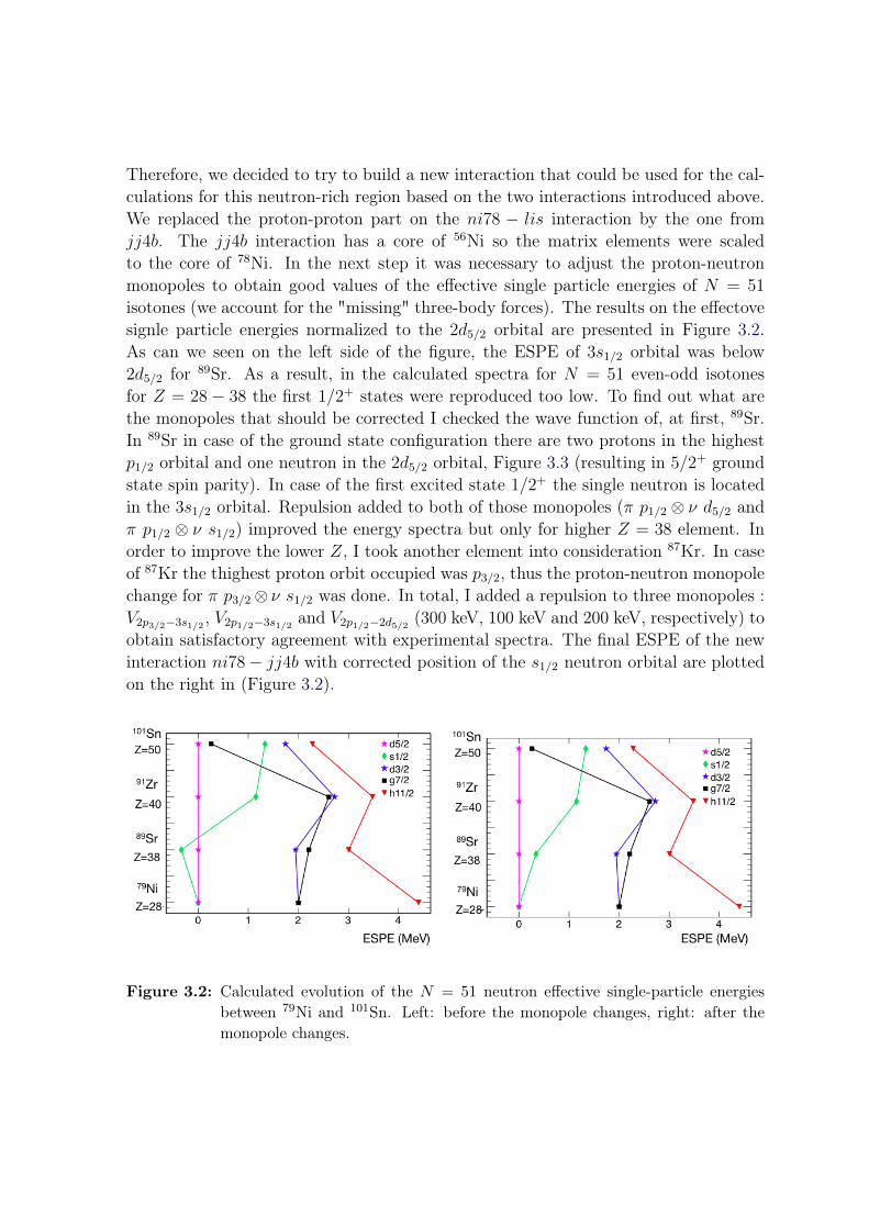
Therefore, we decided to try to build a new interaction that could be used for the cal-culations for this neutron-rich region based on the two interactions introduced above.We replaced the proton-proton part on the ni78 − lis interaction by the one fromjj4b. The jj4b interaction has a core of 56Ni so the matrix elements were scaledto the core of 78Ni. In the next step it was necessary to adjust the proton-neutronmonopoles to obtain good values of the effective single particle energies of N = 51

isotones (we account for the "missing" three-body forces). The results on the effectovesignle particle energies normalized to the 2d5/2 orbital are presented in Figure 3.2.As can we seen on the left side of the figure, the ESPE of 3s1/2 orbital was below2d5/2 for 89Sr. As a result, in the calculated spectra for N = 51 even-odd isotonesfor Z = 28 − 38 the first 1/2+ states were reproduced too low. To find out what arethe monopoles that should be corrected I checked the wave function of, at first, 89Sr.In 89Sr in case of the ground state configuration there are two protons in the highestp1/2 orbital and one neutron in the 2d5/2 orbital, Figure 3.3 (resulting in 5/2+ groundstate spin parity). In case of the first excited state 1/2+ the single neutron is locatedin the 3s1/2 orbital. Repulsion added to both of those monopoles (π p1/2 ⊗ ν d5/2 andπ p1/2 ⊗ ν s1/2) improved the energy spectra but only for higher Z = 38 element. Inorder to improve the lower Z, I took another element into consideration 87Kr. In caseof 87Kr the thighest proton orbit occupied was p3/2, thus the proton-neutron monopolechange for π p3/2⊗ ν s1/2 was done. In total, I added a repulsion to three monopoles :V2p3/2−3s1/2 , V2p1/2−3s1/2 and V2p1/2−2d5/2 (300 keV, 100 keV and 200 keV, respectively) toobtain satisfactory agreement with experimental spectra. The final ESPE of the newinteraction ni78− jj4b with corrected position of the s1/2 neutron orbital are plottedon the right in (Figure 3.2).

Figure 3.2: Calculated evolution of the N = 51 neutron effective single-particle energiesbetween 79Ni and 101Sn. Left: before the monopole changes, right: after themonopole changes.

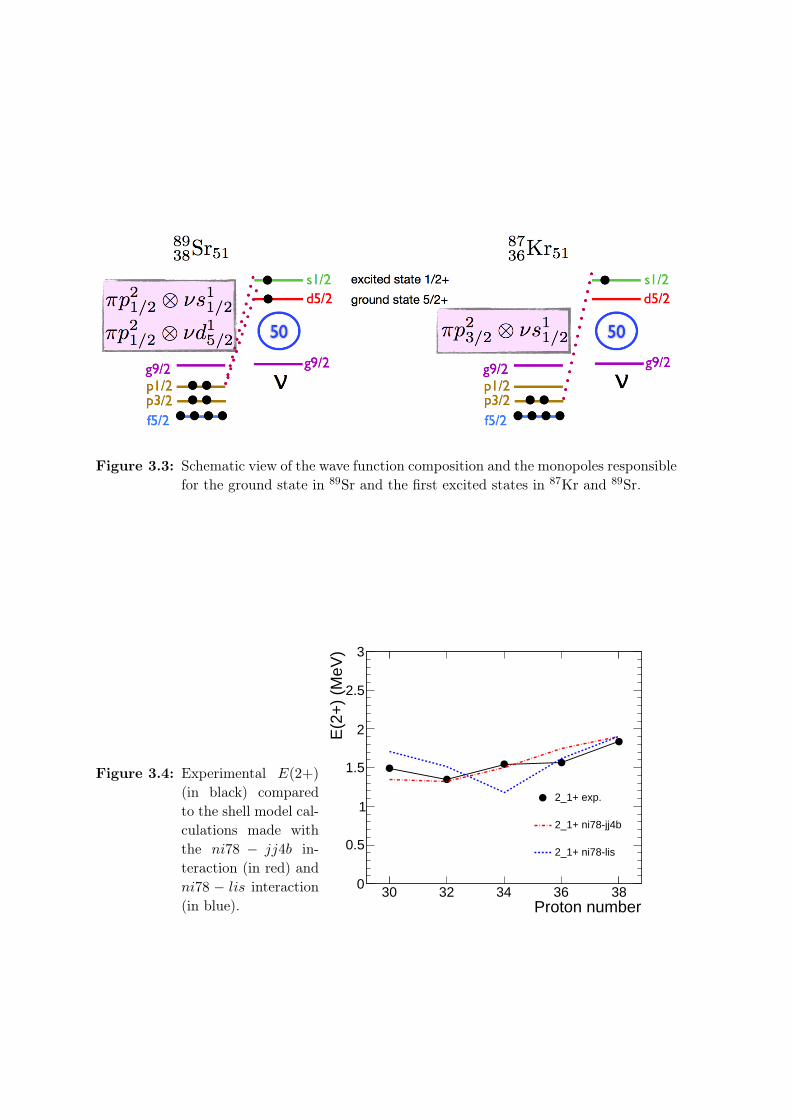
Figure 3.3: Schematic view of the wave function composition and the monopoles responsiblefor the ground state in 89Sr and the first excited states in 87Kr and 89Sr.

Figure 3.4: Experimental E(2+)

(in black) comparedto the shell model cal-culations made withthe ni78 − jj4b in-teraction (in red) andni78 − lis interaction(in blue). Proton number

30 32 34 36 38

E(2

+)

(MeV

)

0

0.5

1

1.5

2

2.5

3

2_1+ exp.

2_1+ ni78-jj4b

2_1+ ni78-lis

Proton number30 32 34 36 38

B(E

2+->

0+)

(e2f

m4)

0

50

100

150

200

250

300

experiment

ni78-jj4b p=1.6 n=0.6

ni78-lis p=1.5 n=0.5

Figure 3.5: The B(E2; 2+→ 0+)

values in the N = 50

isotonic chain com-pared to the shellmodel calculationsmade with theni78 − jj4b inter-action in red andni78 − lis interactionin blue. To reproducethe experimentalresults the effectivecharge of protonsin the ni78 − jj4b

interaction was set to1.6.

The spectra for N = 50 isotones are presented in Figure 3.4 and Figure 3.6. As ex-pected the spectra obtained with the ni78− jj4b interaction does not differ a lot fromthose with the jj4b interaction (as they have the same proton part). The differencescome only from the density dependence which is present in the jj4b interaction but notin ni78− jj4b. The new ni78− jj4b interaction reproduced well the low lying spectraof N = 50 even-even and even-odd systematics. It gives also satisfactory results forN = 52 isotonic chain (Figure 3.8). It reproduces well the ground state spins andparities for N = 50, 52 isotones as well as the low-lying excited states. The perfor-mance of the new interaction was also tested with the reduced transition probabilitiesfor N = 50 isotonic chain (Figure 3.5). To reproduce well the B(E2) values the ef-fective charges for proton and neutron were set to πe = 1.6 πν = 0.6. Through thoseeffective charges one accounts for the effect of core polarization so the contribution ofthe protons and neutrons from the core to the excitations of valence quasi-particles.

To conclude, we consider the ni78− jj4b interaction as a good interaction which willbe used in the proceeding chapters to describe the low-lying states in energy spectraof our nuclei of interest.

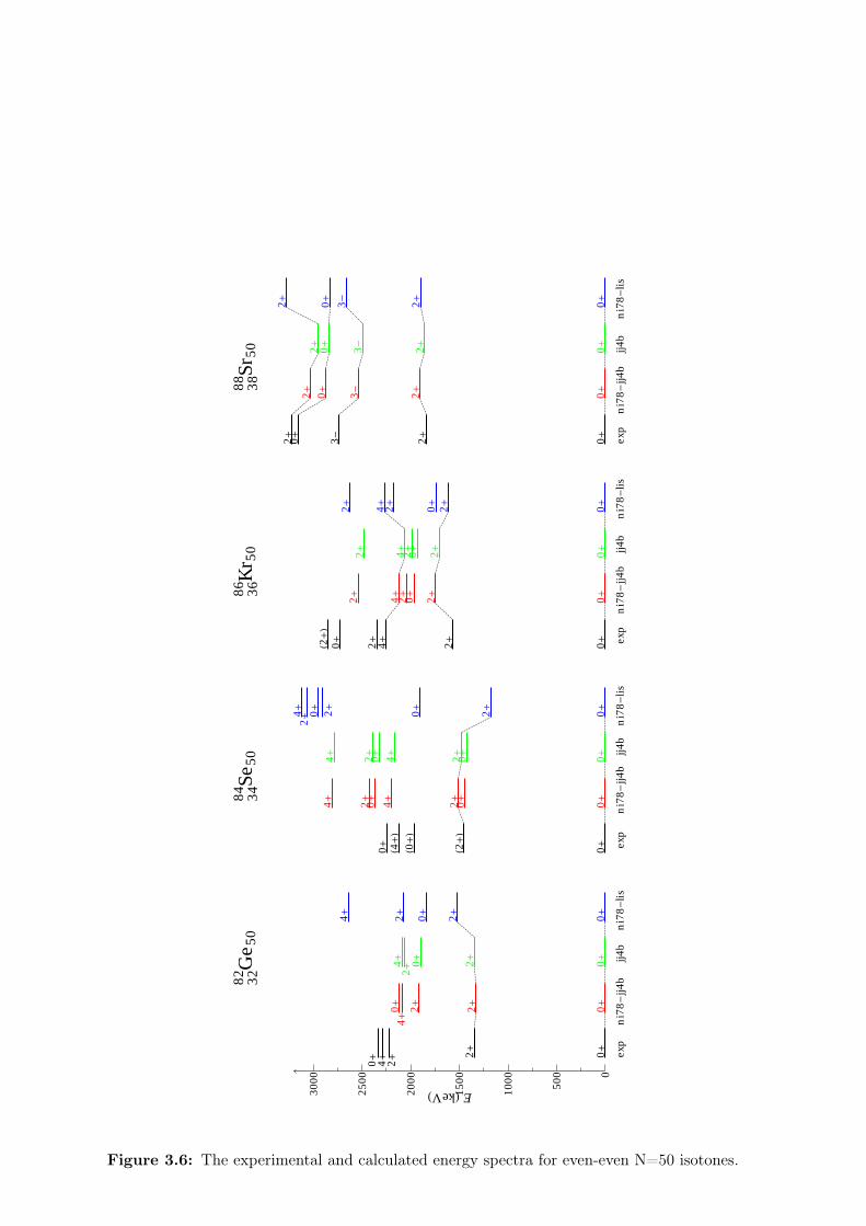
0

500

1000

1500

2000

2500

3000

EHkeVL

0+2+

0+2+2+0+

0+2+0+4+

0+2+0+2+4+

0+H2+L

H0+L

H4+L

0+

0+0+2+4+0+2+4+

0+0+2+4+0+2+4+

0+2+0+0+4+

0+2+4+2+0+H2+L

0+2+0+2+4+2+

0+2+0+2+4+2+

0+2+0+2+4+2+

0+2+3-0+2+

0+2+3-0+2+

0+2+3-0+2+

0+2+3-0+2+

2+4+0+

4+2+

2+

2+

exp

ni7

8-jj4

bjj4

bn

i78-

lis

exp

ni7

8-jj4

bjj4

bn

i78-

lis

exp

ni7

8-jj4

bjj4

bn

i78-

lis

exp

ni7

8-jj4

bjj4

bn

i78-

lis

3282G

e 50

3484Se

503686

Kr 5

03888

Sr50

Figure 3.6: The experimental and calculated energy spectra for even-even N=50 isotones.

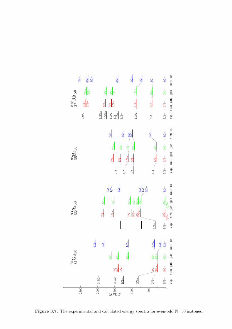
0

500

1000

1500

2000

2500

EHkeVL

52-

32-

32-

92-

3,52

-

3,52

-

52-

32-

32-

12-

92-

72-

52-

32-

32-

52-

92-

52-

52-

32-

32-

12-

72-

92-

52-

12-

32-

12-

32-

72-

12-

72-

32-

12-

32-

72-

12-

72-

32-

12-

32-

52-

72-

32-

52-

32-

12-

72-

32-

52-

32-

12-

52-

72-

32-

52-

32-

12-

52-

72-

32-

52-

32-

12-

52-

72-

32-

52-

1,32

-

32-

12-

1,32

-

3,52

-

1,32

-

7,92

-

32-

52-

12-

32-

52-

72-

32-

52-

12-

32-

52-

72-

32-

52-

12-

12-

32-

52-

32-

72-

52-

12-

52-52

-

52-52

-

92-

12-

32-

12-

32-

exp

ni7

8-jj4

bjj4

bn

i78-

lis

exp

ni7

8-jj4

bjj4

bn

i78-

lis

exp

ni7

8-jj4

bjj4

bn

i78-

lis

exp

ni7

8-jj4

bjj4

bn

i78-

lis

3181G

a 50

3383A

s 50

3585B

r 50

37878 R

b50

Figure 3.7: The experimental and calculated energy spectra for even-odd N=50 isotones.

0

500

1000

1500

2000

2500

EHkeVL

0+2+

0+2+2+4+0+2+3+0+3+

0+2+4+0+5+4+3+

0+H2+L

H4+L

H6+L

0+2+4+2+0+2+0+4+4+6+

0+2+4+2+0+2+0+4+6+

0+2+2+4+2+H3,4+

L

0+2+4+2+0+2+4+4+

0+2+4+0+2+0+4+4+

0+2+4+2+3-

0+2+4+2+0+2+4+3-

0+2+4+2+2+0+4+0+3-

4+

2+3+

0+

2+

0+

exp

ni7

8-jj4

bn

i78-

lis

exp

ni7

8-jj4

bn

i78-

lis

exp

ni7

8-jj4

bn

i78-

lis

exp

ni7

8-jj4

bn

i78-

lis

3284G

e 52

3486Se

523688

Kr 5

23890

Sr52

Figure 3.8: The experimental and calculated energy spectra for even-even N=52 isotones.From left: experimental values, calculated with ni78 − lis and ni78 − jj4b

interactions.

Chapter 4

Development of an experimentalsetup to characterize the release of

UCx target prototypes

Contents4.1 Study of the feasibility of the experiment . . . . . . . . . . . . 35

4.1.1 Simulation . . . . . . . . . . . . . . . . . . . . . . . . . . . . . . . 38

4.1.2 The simulated spectrum and its interpretation . . . . . . . . . . . 43

4.2 The experiment . . . . . . . . . . . . . . . . . . . . . . . . . . . 45

4.2.1 Description of the experiment . . . . . . . . . . . . . . . . . . . . 45

4.2.2 Exploitation of the calculations and measured spectra . . . . . . 46

4.1 Study of the feasibility of the experiment

Over the last two decades, facilities using ISOL (Isotope Separation On-Line) havebeen developing around the world: ISOLDE (CERN), TRIUMF (Canada), SPIRAL(France), HRIBF (USA) etc. Those facilities have proved their capability to efficientlyproduce a variety of beams. This is confirmed by today’s international projects forthe construction of second generation ISOL facilities: SPIRAL2, EURISOL-DS, SPESetc. These projects focus on the development of neutron-rich isotope beams obtainedfrom the irradiation of well-designed fission targets. The target is indeed the elementat the heart of an ISOL installation. In 2002, a European project TARGISOL wasdedicated to the creation of a general database for the optimization of ISOL targets.Experimental work has been initiated to develop UC targets in the framework of theEuropean projects SPIRAL2 and EURISOL-DS.

The research and development (R&D) programme PARRNe (Production d’AtomesRadioactifs Riches en Neutrons) at the Institute of Nuclear Physics in Orsay (IPNO)is devoted to studying the production of neutron-rich fission fragment beams extracted

from the thick targets [79] produced to an ISOL design (e.g. [80]). The continuousdevelopment of the targets is required since all chemically “easy” beams are alreadyin use and the experiments are pursued far from the valley of beta-stability, where of-ten one has to work with extremely short half-lives and low production cross-sections.This development concentrates at present on creating a more solid understanding ofthe performance of the target in order to reduce the decay losses and make beams ofthe remaining elements available [81]. Various materials have been tested and used asISOL targets. The release properties of UCx and molten U thick targets have beenstudied at PARRNe [82, 83]. Such developments are fundamental for the next gen-eration of ISOL facilities. The current study carried out at IPNO is in particularsupported by the SPIRAL2 project.

At present, the target PARRNe used at ALTO consists of 160 pellets of UCx (x indi-cates an excess of graphite), each 1 mm thick. The geometrical density of the pellet is3.5 g/cm3 (measured volume includes pores). The design of the standard fission targetfor SPIRAL2 is based on the pellets used at ALTO. This standard target would becomposed of 19 x 80 UCx pellets. For this target the fission yield is estimated to bein the order of 1013 fission/s [84]. One of the goals of the R&D programme at IPNOrsay in collaboration with Laboratory of Chemical Science in Renne, is to produce amaterial which would allow one to obtain up to 1014 fission/s. The amount of uraniumand the porosity of the target influence essentially the final flux of the fission products.The higher density of the uranium increases the production rate and at the same timeprohibits the radioactive elements from easily leaving the target, while the efficiencyof the release of elements depends on the porosity of the material. Thus the bestcompromise between these two factors will be found to design the target of interest.This compromise requires an investigation of the manufacturing processes. The pel-lets differ from each other by the amount of uranium and the structure. Those pelletsare produced within an internal collaboration between ALTO and the radiochemistrygroup at IPN Orsay.

We aimed to perform an experiment which would allow us to compare the releaseproperties of differently manufactured UCx pellets. In order to find out which of thepellets has better release properties and could be used in future experiments with ra-dioactive beams.The basic procedure is as follows:

1. Production of radioactive species in the UCx target.Two identical UCx pellets are irradiated with fast neutrons to induce fission (seeChapter 5). Those fast neutrons are produced by impinging the 26 MeV deuteronbeam delivered by the tandem accelerator on the graphite converter placed infront of the first pellet.

2. Heating one of the pellets up to high temperature.The radioactive fission product does not leave the target of its own accord. Inorder for the elements of interest to effuse from the target the pellet should beheated to a high enough temperature. In this step of the experiment one ofthe pellets is placed in a tubular oven and heated for about 30 min to allowthe elements to effuse. The second pellet is placed in a plastic container, thusprepared for the further measurement as a reference.

3. Measurement of the radioactivities and data analysis.After heating, each pellet is placed in front of a germanium detector and theactivities are measured. The pop-tops of the detectors are covered with leadshields in order to avoid background radiation. The pellet which has been heatedis expected to be less radioactive than the non-heated one, since due to theheating some elements effused from it. Thus the gamma spectra should not beidentical and some differences are expected to be visible. An identification ofthe isotopes is made through their γ−lines. From further analysis of the dataone should be able to deduce which elements effused during heating and howabundantly. Moreover, since the same experimental procedure is used for thedifferent sets of UCx pellets, we shall find out which manufacturing method isthe most efficient when it comes to production of the target with the best releaseproperties.

The short-lived (ns to s) radioactive species created by fission induced by fast neutronswill decay towards longer-lived isobars emitting β and γ radiations. The experimentwas planned to be performed without mass selection, thus, one must be aware of thecomplexity of the spectra which will contain γ -lines from all the radioactive elementspresent in the target at the time of measurement. The measurement of the radioactiv-ities is done after heating, that is, when the initial fission products will already havedecayed to their daughters.

Several aspects had to be considered before the experiment as many fission productswere expected. Will it be possible to find well identified γ -lines with high statistics toidentify the elements? After over about half-hour heating will there be enough activityin the pellets? There are also other factors, like the time of irradiation or the time ofmeasurement, that should be planned and optimized:

• tirr (tirradiation): the time for which two pellets are irradiated. The irradiationtime should be long enough to produce many radioactive elements but not toolong for the activity of the pellets to be too high for manipulation and counting.The measurement with germanium detectors will be performed at least half anhour after the irradiation so only the radioactive elements with half-lives of afew minutes and longer will be counted. Taking all these factors into accountthe time of irradiation was first estimated to be 30 minutes.

• twait: the total time needed for the manipulation of the pellets after the irradi-ation and heating one of them in the oven for approximately 30 min. A priorithe "waiting" time was foreseen to be 45 minutes.

• tmeas (tmeasurement): the time required to measure the pellets using two HPGedetectors. Taking into account the duration of heating we are considering ele-ments with few minutes half-lives. The time of counting should be long enoughto have sufficient statistics while the activity of the pellets is still high enough.

• detection system: two HPGe detectors will be used to measured both pelletssimultaneously. The acceptance of the detector is about 20000 c/s and too highan activity of the pellets can disable the detector. This factor may be controlledby putting the pellet further from the crystal.

To demonstrate feasibility and plan the experiment, a simulation of the γ-spectrumwas made. It played a crucial role before making the measurement. The goal of thesimulation was to study the feasibility of the experiment by evaluating the complexityof the spectrum and determining the release of which elements of interest we can expectto study. We needed to predict how the spectrum recorded after heating would lookwhen measured for 1 h if there are enough radioactive elements and if the various peakswould be identifiable, thus, if the identification of certain elements of interest will bepossible. Furthermore, the calculations would prove whether an irradiation time of30 minutes is feasible and whether the counting rate will be below the acceptance ofthe detector.

4.1.1 Simulation

Production of radioactive species

During the irradiation, radioactive elements are produced at a given rate. This rate Rwill depend on the number of target atoms Na, of the flux of incident particle I andon the reaction cross section σ:

R = NaσI .

After the nuclei are formed they decay according to the exponential law of radioactivedecay

N(t) = N0 · eλt

where N0 gives the original number of nuclei present at time t = 0 and λ = ln2t1/2

wheret1/2 is the half-live, the time necessary for half of the nuclei to decay.

Let us assume the following situation: we have a target of stable nuclei and we bom-bard it with the beam of particles. NA is the number of nuclei that are formed as a

result of reactions. Those nuclei decay with decay constant λA to the nuclei denotedby B. The number of nuclei A present increases due to the production rate R anddecreases due to the radioactive decay:

dNA(t)

dt= RA − λANA . (4.1)

Integration of this equation over the time of irradiation (0, tirr) gives the result:

NA(tirr) =RA

λA(1− e−λAtirr) . (4.2)

Since no new activity is formed after irradiation, the radioactive nuclei will decayaccording to the exponential law

NA(twait) =RA

λA(1− e−λAtirr) e−λAtwait , (4.3)

where twait is the time from the end of irradiation until the beginning of the measure-ment. Finally, during the period of the measurement the number of nuclei present isgiven by

NA(tmeas) =RA

λA(1− e−λAtirr) e−λAtwait e−λAtmeas . (4.4)

We are interested in the number of decays of nuclei A during the whole period ofmeasurement (t0, tend) where t0 is the end of the waiting time (t0 = twait) and tend isthe time at the end of the measurement. This can be found by integrating Eq. (4.4):

NA(t0, tend) =

∫ tend

t0

λANA(t) dt , (4.5)

here t0 = 0. Therefore, the total number of disintegrations for nuclei A is:

NA(tend) =RA

λA(1− e−λAtirr) e−λAtwait (1− e−λAtend) . (4.6)

Let us consider the second generation of nuclei which in this case is also radioactiveand has a decay constant λB. The number of daughter nuclei NB present increases asa result of decays of the parent and decreases as a result of its own decay:

dNB(t)

dt= λANA − λBNB . (4.7)

Solving Eq. (4.7) in the same manner as for mother nuclei one obtains the solution forthe number of decays of the daughter nucleus during the whole measurement period:

NB(tend) =RAλB

λA(λB − λA)(1− e−λAtirr) e−λAtwait (1− e−λAtend)

− RAλAλB(λB − λA)

(1− e−λBtirr) e−λBtwait (1− e−λBtend) .(4.8)

The same equations can be solved for the third, fourth and nth generations until onereaches the stable nucleus or, as in our case, the half-live of the nth daughter is longenough to be ignored.

Figure 4.1: Production of radioactive species. Scheme of decay chains.

In our target not only nuclei A are produced but also B, C .. up to a few generations.The direct production of the daughter in the target should also be taken into accountfor the final number of disintegrations of this element during the measurement. In thiscase the total number of disintegrations will consists of both : decay of the elementsproduced by the decay of the parent and decay of the elements which were produced inthe target (Figure 4.1). Thus, in the next step B will be the primary nuclei producedin the target with the production rate RB. One can apply the same procedure for thecalculation starting from the equation (4.1) this time for the nuclide B. The samecan be done for all the generations of interest and the final number of disintegrationsof the elements of interest will be the sum of disintegrations calculated from all theconsidered chains.

Case of several generations: Bateman equations

If we assume that there are several succeeding generations of radioactive nuclei wecan write

dNi(t)

dt= λi−1Ni−1 − λiNi . (4.9)

We consider the simplified case where at the initial time t = 0 only the parent nuclideis present Ni=1,0 6= 0 and none of the other types. Bateman [85] has given the solution

for a chain of n members with this assumption:

Nn(t) =n∑i=A

Cie−λit

= (CAe−λAt + CBe

−λBt + . . . Cne−λnt) ,

(4.10)

where C is a constant having the form

Cm =

n∏i=A

λi

n∏i=A

(λi − λm)

Ni=1,0 (i 6= m)

=λAλB . . . λn

(λA − λm)(λB − λm) . . . (λn − λm)Ni=1,0 .

(4.11)

Let us demonstrate it for the case studied before:

Ni=A,0 = NA(twait)

=RA

λA(1− e−λAtirr) e−λAtwait .

(4.12)

NA(t) = NA(tmeas) =RA

λA(1− e−λAtirr) e−λAtwait e−λAtmeas . (4.13)

Integrating over the period of measurement (t, tend) one recovers Eq. (4.6). The samecan be applied for the subsequent generations.

Details of the simulation

The conditions for the simulation were taken as follows: tirr=30 min, twait=45 minand tmeas=60 min. As mentioned before, the fission products are very short-livedand most of them will decay before the detection. What will be measured in thespectrum are γ-lines coming not from the parents but their decay products (daughtersand grand-daughters even up to a few generations). The nuclei taken into accountfor calculation must be γ emitters with half-lives of minutes. The spectrum containsγ -lines from 62 radioactive elements (Tab.4.1). For the calculation of the number ofdisintegrations of the elements of interest the Bateman equations were used. The γ -lines were simulated as gaussian-shaped peaks. The simulation was made with ROOTin a first approximation of the full energy peak (without Compton, backscattering,Bremsstrahlung). For the simulation the resolution of the detector was assumed to bea linear function of energy y = a · Eγ + b where a = 0.0003 and b = 0.6497. Thosecoefficients were calculated assuming that the resolution of the germanium detector is1.6 keV and 2.5 keV at 100 keV and 1.3 MeV γ -rays, respectively.

Table 4.1: Radioactive nuclids used in the simulation. Half-lives are taken from ([86]) andthe independent yields from [87].

Element Half-life Independent yield [%] Element Half-life Independent yield [%]87Kr 76.3 m 8.28E-002 128mSb 10.4 m 1.02E-00188Kr 2.84 h 5.57E-001 129Sb 2.23 m 5.56E-00188Rb 17.77 m 1.50E-002 129Te 69.6 m 4.19E-00389Rb 15.15 m 1.11E-001 130Sb 39.5 m 7.43E-00191Sr 9.34 h 6.95E-002 131Sb 23.3 m 2.49E+000

91mY 49.71 m 0.00E+000 131Te 25 m 9.78E-00292Sr 2.71h 2.63E-001 132Te 3.204 d 1.46E+00092Y 3.54 h 0.00E+000 132I 2.29 h 1.86E-00193Y 10.18 h 3.06E-002 133mTe 55.4 m 2.54E+00094Y 18.7 m 1.65E-001 133Te 12.4 m 5.58E-00195Y 10.3 m 5.98E+000 133mI 9 s 0.00E+00097Zr 16.91 h 3.46E-001 133I 20.8 h 4.68E-001

97mNb 52.7 s 4.34E-004 134Te 41.8 m 3.72E+00097Nb 72.1 m 3.51E-003 134I 52.5 m 5.97E-00199Mo 65.04 h 1.13E-003 135I 6.57 h 2.57E+000101Mo 14.61 m 6.02E-002 135mXe 15.29 m 2.02E-001101Tc 14. 2m 2.14E-004 135Xe 9.13 h 2.02E-001102Mo 11.3 m 2.08E-001 138Xe 14.08 m 1.85E+000102Tc 5.28 s 9.33E-004 138Cs 33.41 m 1.74E-001104Tc 18.3 m 6.75E-002 139Cs 9.27 m 1.39E+000105Ru 4.44 h 2.82E-003 139Ba 83.06 m 2.72E-001

105mRh 45 s 1.11E-007 141Ba 18.27 m 5.19E-001107Rh 21.7 min 1.35E-004 141La 3.92 h 7.98E-003117Cd 2.49 h 2.62E-004 142Ba 10.6 m 1.11E+000

117mIn 116.2 m 3.46E-006 142La 91.1 m 4.62E-002117In 43.2 m 3.46E-006 143La 14.2 m 1.88E-001118In 5 s 4.70E-005 143Ce 33.03 h 1.80E-003

123mSn 40.06 m 1.02E-003 146Ce 13.5 m 2.19E-002125mSn 9.52 m 2.19E-002 146Pr 22.15 m 3.57E-003

127Sn 2.1 h 5.46E-001 147Pr 13.4 m 2.22E-002128Sn 59.07 m 1.13E+000 149Nd 1.7 h 6.28E-003

4.1.2 The simulated spectrum and its interpretation

The simulated spectrum corrected for the efficiency of the detector is presented inFigure 4.2. Although the spectrum contains many peaks, there are several that arewell separated, pure and of high statistics. The estimated counting rate was 12000 c/swhich is high enough to get good statistics during the measurement and at the sametime not too high for detection (the acceptance of HPGe detectors 20000 c/s). Theirradiation time estimated for the purpose of the simulation is sufficient and there arewell separated peaks which can be identified from the measured spectra. Thus onecan conclude that these experimental conditions are sufficient to perform successfulmeasurements.

Table 4.2: The γ -lines ([86]) of the elements of interest identified in the spectrum Figure 4.2.

Element Energy [keV] T 12[86] Element Energy [keV] T 1

2[86]

135Xe 249.77 9.13 h 129Te 27.81 69.6 m138Xe 1768.26 15.29 m 134Te 79.45 41.8 m138Cs 1435.8 33.41 m 134Te 201.24 41.8 m138Cs 2218 33.41 m 134Te 565.99 41.8 m138Cs 2639.59 33.41 m 133mTe 334.27 55.4 m134I 235.47 52.5 m 133mTe 863.96 55.4 m135I 288.45 6.57 h 133mTe 1683.23 55.4 m134I 514.4 52.5 m 133Te 1881.52 12.5 m134I 595.36 52.5 m 88Kr 196.3 2.84 h134I 847.03 52.5 m 87Kr 402.59 76.3 m134I 884.09 52.5 m 88Kr 1529.77 76.3 m132I 954.55 2.29 h 88Kr 2195.84 2.84 h134I 974.67 52.5 m 88Kr 2392.11 2.84 h134I 1072.55 52.5 m 87Kr 2554.8 76.3 m135I 1131.51 6.57 h 88Rb 1836.06 17.77 m134I 1613.8 52.5 m 89Rb 2570.19 15.15 m135I 1791.2 6.57 h135I 1791.2 6.57 h134I 1806.84 52.5 m

Not all elements can escape from the target in the same way (see Chapter 5). Therelease of a given element depends on various physico-chemical parameters which aredifficult to characterize at high temperature. Nevertheless, at a temperature of 1200 Cwe expect to observe the release of the most volatile elements such as alkalis andnoble gases. Other less volatile elements which are produced in great amounts arealso expected. At 1200 C the elements that can evaporate from the target are mostly

alkalies (e.g. Rb, Cs) and noble gases (e.g. Kr, Xe) Figure5.11. The gamma peaks ofidentified elements are indicated in the spectrum (Fig. 4.2, Table 4.2) and are potentialcandidates for identification in the experimental spectra.

Figure 4.2: The simulated spectrum of the fission products produced in the uranium car-bide target. It presents the prediction of the target activity measured 45 minafter irradiation. The measurement time is one hour. The spectrum has beencorrected for the detector efficiency. γ -lines of Kr (?), Xe (5), Te (4), Cs (©),I () and Rb (×) are identified.

4.2 The experiment

4.2.1 Description of the experiment

The deuteron beam of energy 26 MeV and intensity 20 nA was delivered using the15MV tandem accelerator. The 3 mm graphite (neutron) converter was placed infront of the first UCx pellet. The pellets were irradiated in pairs placed one behindthe other. The scheme of the experimental procedure is presented in Figure 4.3.

Different methods of target synthesis must be investigated. Indeed, the physico-chemical properties of the pellet depends directly on the synthesis process. It wasfirst decided to explore two different synthesis methods:

• UCx pellets synthesized by the carbo-reduction method

• UC pellets synthesized by the arc melting method

The advantage of the first method is that it is possible to have a large variety ofdifferent compositions depending on the chemical components involved. For instance,standard pellets used at ALTO and named PARRNe have been obtained by the carbo-reduction of uranium oxide and carbon. To improve the porous structure of the targeta prototype has been developed by inserting a certain amount of carbon fibers. Theprototype containing 30% of those fibers has been named COM30. In the secondmethod an electric arc is used to melt a blend of carbon and uranium (ARC melting).The interest of this method is to have a pure UC target in order to reach the highestconcentration of uranium in the target. The disadvantage however is, as mentionedbefore, that the higher the uranium density in the target the more compact the targetwill be, which is not favorable for release.

Step 1. The irradiation.In the first step the targets were irradiated in couples (e.g. COM30.P1 andCOM30.P2). The first couple of pellets was irradiated as previously plannedfor 30 min. Unfortunately, the overall activity generated in the setup did notallow us to extract safely the pellets for identification and heating for 1 hour.For safety reasons the extraction was allowed only when the overall dose ratewas below 20 mSv/h. In fact, when it became possible to extract the pellets, wefound that the strong radioactivity observed was in great part coming from themetallic system used as a fast removable support for the pellets. The decisionwas made to shorten the irradiation time to 20 min with a beam intensity of20 nA.

Step 2. Measurement of the activities.The radioactivities of two pellets were measured for 10 min with HPGe detectors.

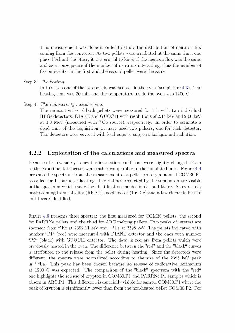
This measurement was done in order to study the distribution of neutron fluxcoming from the converter. As two pellets were irradiated at the same time, oneplaced behind the other, it was crucial to know if the neutron flux was the sameand as a consequence if the number of neutrons interacting, thus the number offission events, in the first and the second pellet were the same.

Step 3. The heating.In this step one of the two pellets was heated in the oven (see picture 4.3). Theheating time was 30 min and the temperature inside the oven was 1200 C.

Step 4. The radioactivity measurement.The radioactivities of both pellets were measured for 1 h with two individualHPGe detectors: DIANE and GUOC11 with resolutions of 2.14 keV and 2.66 keVat 1.3 MeV (measured with 60Co source); respectively. In order to estimate adead time of the acquisition we have used two pulsers, one for each detector.The detectors were covered with lead cups to suppress background radiation.

4.2.2 Exploitation of the calculations and measured spectra

Because of a few safety issues the irradiation conditions were slightly changed. Evenso the experimental spectra were rather comparable to the simulated ones. Figure 4.4presents the spectrum from the measurement of a pellet prototype named COM30.P1recorded for 1 hour after heating. The γ -lines predicted by the simulation are visiblein the spectrum which made the identification much simpler and faster. As expected,peaks coming from: alkalies (Rb, Cs), noble gases (Kr, Xe) and a few elements like Teand I were identified.

Figure 4.5 presents three spectra: the first measured for COM30 pellets, the secondfor PARRNe pellets and the third for ARC melting pellets. Two peaks of interest arezoomed: from 88Kr at 2392.11 keV and 142La at 2398 keV. The pellets indicated withnumber “P1“ (red) were measured with DIANE detector and the ones with number“P2“ (black) with GUOC11 detector. The data in red are from pellets which werepreviously heated in the oven. The difference between the ”red” and the ”black“ curvesis attributed to the release from the pellet during heating. Since the detectors weredifferent, the spectra were normalized according to the size of the 2398 keV peakin 142La. This peak has been chosen because no release of radioactive lanthanumat 1200 C was expected. The comparison of the ”black” spectrum with the ”red“one highlights the release of krypton in COM30.P1 and PARRNe.P1 samples which isabsent in ARC.P1. This difference is especially visible for sample COM30.P1 where thepeak of krypton is significantly lower than from the non-heated pellet COM30.P2. For

P2

P1

Figure 4.3: Up: Scheme of steps for experimental procedure. Middle: a UCx pellet in theoven. Bottom: germanium detector with pellet placed on the support systemin front of the crystal

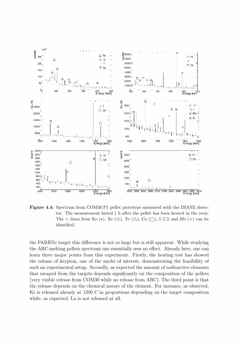
Figure 4.4: Spectrum from COM30.P1 pellet prototype measured with the DIANE detec-tor. The measurement lasted 1 h after the pellet has been heated in the oven.The γ -lines from Kr (?), Xe (5), Te (4), Cs (©), I () and Rb (×) can beidentified.

the PARRNe target this difference is not so large but is still apparent. While studyingthe ARC-melting pellets spectrum one essentially sees no effect. Already here, one canlearn three major points from this experiment. Firstly, the heating test has showedthe release of krypton, one of the nuclei of interest, demonstrating the feasibility ofsuch an experimental setup. Secondly, as expected the amount of radioactive elementsthat escaped from the targets depends significantly on the composition of the pellets(very visible release from COM30 while no release from ARC). The third point is thatthe release depends on the chemical nature of the element. For instance, as observed,Kr is released already at 1200 C in proportions depending on the target compositionwhile, as expected, La is not released at all.

Figure 4.5: Comparison of the release fraction of krypton from pellets: COM30, PAR-RNe and ARC-melting. Left peak 88Kr (2392.11 keV) and right peak 142La(2398 keV). The data from the two detectors were normalized according to thesize of the peak of lanthanum.

The feasibility of the experiment studied with the simulation was confirmed and thesimulated spectrum was found to be very useful when studying the measured ones.The second experiment to study the release properties of different prototypes of UCx tar-gets have been carried out with 1500 C heating temperature. The first results withthe detailed release fractions from the first and the second experiment were recentlypublished [88]. The three pellets OXA, COM30 and PARRNe were found to havethe highest release fraction but the interpretation of the material properties is still inprogress. Most importantly, it was demonstrated that the experimental method tostudy differently pellets was confirmed.

For the future developement of the target more new prototypes will be developedand the heating temperature should be increased to be as close as possible to the op-erating temperature at ALTO and SPIRAL2 (2000 C). A big part of any future workwill concentrate on the material synthesis for new target prototypes.

Chapter 5

Production of radioactive ion beams

Contents5.1 Production methods . . . . . . . . . . . . . . . . . . . . . . . . . 51

5.2 Production of radioactive nuclei with fission reaction . . . . . 53

5.2.1 Neutron-induced fission . . . . . . . . . . . . . . . . . . . . . . . 53

5.2.2 Photo-fission . . . . . . . . . . . . . . . . . . . . . . . . . . . . . 54

5.3 Ion sources . . . . . . . . . . . . . . . . . . . . . . . . . . . . . . 57

5.4 The ALTO facility . . . . . . . . . . . . . . . . . . . . . . . . . . 61

5.4.1 LINAC . . . . . . . . . . . . . . . . . . . . . . . . . . . . . . . . 62

5.4.2 Target and the ion source . . . . . . . . . . . . . . . . . . . . . . 63

5.4.3 The laser ion source at ALTO . . . . . . . . . . . . . . . . . . . . 64

5.4.4 Mass separator PARRNe . . . . . . . . . . . . . . . . . . . . . . . 68

5.1 Production methods

There are different methods to produce neutron or proton radioactive ion beams:multi-nucleon transfer reactions, induced fission, spallation and fragmentation reac-tions. The choice of reaction mechanism depends on the region of interest. After theirproduction, the nuclei of interest must be separated from other reaction products.There exist two separation techniques: In-Flight Separation and Isotope SeparationOn Line.

In-Flight Separation

The In-Flight (IF) separation method can be explained on the fragmentation reaction.The high-energy heavy-ion projectiles bombard a thin target (less than a gram/cm2)and radioactive isotopes are produced through the fragmentation reaction. The tar-get should be as thin as possible to avoid absorption of the reaction products and tonarrow their energy distribution. The nuclei leave the target highly ionized and areseparated in-flight by means of magnetic and/or electric fields. This method provides

us with so-called “cocktail“ beams and specific nuclides can be selected according totheir atomic number and atomic mass. In this method the produced nuclei are avail-able instantly. However, the products are often highly energetic (hundreds of MeVper nucleon) which is suitable for reaction studies but too high for nuclear structurestudies. They may have a broad energy distribution, often large angular divergenceand their purity is rather poor.

There are a number of facilities worldwide which are based on this technique, likethe FRS facility at GSI (Darmstadt, Germany), LISE at GANIL (France), COMBASat FLNR (Dubna, Russia), the fragmentation facilities at MSU (Michigan, USA) andat RIKEN (Japan).

Isotopic Separation On-Line

In the ISOL method an intermediate- or heavy-mass thick target is bombarded withlight beam (neutrons, protons, electrons or γ -rays). Various kinds of reaction can beinduced: if the energy of the primary beam is low (a few tens of MeV per nucleon)fusion-evaporation, fission, or multi-nucleon transfer reactions, or in case of a highlyenergetic projectiles (e.g., a few hundreds of MeV for neutrons or around 1 GeV forprotons) fragmentation and spallation. In this technique the radionuclides are stoppedin the target from which they are subsequently released by diffusion in the target ma-terial and desorption from the material surface while heating the target to sufficientlyhigh temperatures. The radionuclides can diffuse out of the target and effuse eventu-ally through a transfer line to the ion source where they are ionized. Using the ISOLtechnique one can produce good-quality beams of nuclei of interest. The beam has avery low energy spread, which allows for a possibility of post-acceleration of the beam,and small angular divergence. This method has also some disadvantages, for instance,a relatively long extraction time which makes the study of many short-lived nuclearspecies almost impossible. The exotic nuclides are produced in limited amounts, thusthe release has to be as efficient as possible, i.e. the radio-nuclides must reach the ionsource, be ionized, accelerated and mass separated before they decay. The chemicalselectivity introduced by the choice of target is limited.

Some of the most known and advanced beam facilities using proton beams are ISOLDEat CERN (Switzerland), IGISOL at Jyväskylä (Finland), HRIBF at ORNL (Oak-Ridge, USA), SPIRAL at GANIL (France), ISAC at TRIUMF (Vancouver, Canada)and ALTO (IPN Orsay, France).

5.2 Production of radioactive nuclei with fission re-action

Nuclear fission is a process in which a heavy nucleus splits into two lighter nuclei emit-ting several neutrons. The reaction is exothermal since the nuclear binding energy pernucleon for the produced medium mass nuclei is significantly higher than the bindingenergy of the original nucleus. To be able to fission, the nucleus has to first stretchto a very elongated shape. It requires energy to deform the nucleus to the so-calledsaddle point, after which the energy is released. The energy may be brought to thenucleus as electromagnetic radiation (photofission) or via a particle (e.g., protons orneutrons). There is a potential barrier against the fission which height for mediumheavy nuclei is of the order of 50 MeV, while for actinides (233U, 235U, 239Pu, 241Pu,241Am, etc. ), of the order of 5 MeV.

The research and development (R&D) program PARNNe (Production d’Atoms Ra-dioactifs Riches en Neutrons) was initiated at the Institut de Physique Nucléaired’Orsay (IPN Orsay, France) in 1997. This program was devoted to study the produc-tion of neutron-rich fission fragment beams extracted from the thick target producedwith ISOL method [79]. In the framework of the PARNNe program different tech-niques were used to characterize the release properties of the elements of interest froma UCx target [89, 90]. Together with the R&D program, the physics research of theneutron-rich elements was started [91, 92]. At first, the fission of 238U was inducedwith the deuteron beam provided by the Tandem accelerator (the Orsay Tandem Vande Graff accelerator with nominal voltage 15 MV). In 2005, the construction of theALTO (Accélérateur Linéaire auprès du Tandem d’Orsay) facility was completed andthe first tests with the electron beam were performed. Today, the ALTO acceleratorprovides 50 MeV electron beam of 10µA intensity.

5.2.1 Neutron-induced fission

Various experiments on the thick uranium carbide target (UCx ) bombarded withfast neutrons were performed in IPN Orsay with PARRNe separator [48, 78]. Fastneutrons were produced by impinging the 26 MeV deuteron beam, delivered by Tandemaccelerator, on the graphite converter placed 5 mm to 110 mm from the center of theuranium target. As deuteron has a low binding energy it can break on the converter(for the beam energy of 40 MeV, 0.013 neutrons per deuteron are produced [93]).The protons from the break-up are absorbed by the converter while the neutrons canescape and travel to the uranium carbide target (with an energy of about 0.4 times ofthe incident energy). To optimize the neutron beam energy many studies have beenmade. The measurements of 238U fission cross section were performed by Lestone andGavrin [94]. The results of the measurements are shown in Figure 5.1. The cross

section (Figure 5.1 (right)) for the reaction increases slowly up to 40 MeV neutron fluxenergy. However, there is a saturation in the production with increasing beam energy(Figure 5.1 (left)) [95]). Another important parameter is the selectivity of the fissionfragments. The fission of 238U at low excitation energy is very asymmetric (Figure 5.2).This asymmetry decreases with increasing energy. Simulations by Mirea et al. [96]show that in order to obtain the most neutron-rich fission fragments in the vicinity ofnickel, the energy of the primary neutron beam should not be higher than 20 MeV (eventhough the rate of the deuteron break up is lower than for higher energy). The Tandemaccelerator at IPN Orsay delivers a deuteron beam of energy 26 MeV and intensityof 1µA (which correspons to 10 MeV neutron beam). It allows the production of 109

fissions/s in the target.

Figure 5.1: (Left) Neutron production at 0 as a function of deuteron beam energy [95].(Right) Fission cross section of 238U as a function of neutron energy [94].

5.2.2 Photo-fission

In the photo-fission process fast electrons interact with the atoms and as a result oftheir deceleration continuous spectrum of γ-rays (Bremsstrahlung) is produced. Thoseγ-rays induce fission in the target. It was Diamond et al. [98] and Oganessian et al.[99] who proposed to use the electrons to induce photo-fission in the uranium tar-get. According to Diamond’s calculation with 30 MeV and 100 kW electron beam itis possible of induce more than 1013 fissions/s. It was experimentally validated byOganessian. In his experiment, an 25 MeV and a 0.5 kW electron beam was sent ona tantalum converter to induce fission in a sheet of uranium. The fission rate in the

Figure 5.2: Distribution of fission fragments as a function of the excitation energy of238U [97].

target was measured to be of the order of 1011 fissions/s.

The energy spectrum produced by the electron beam is presented in Figure 5.3 (a)(left-hand scale). As can be seen, the energy of γ generated by the Bremsstrahlungvaries up to a maximum corresponding to the energy of the incident electron beam.The trend increases gradually with the increase of the electron beam energy. To in-duce fission the photons energy must be greater than the fission threshold energy of238 uranium which is 6 MeV. On the right axis the fission cross section is plottedas a function of incident photon energy. The total photon absorption cross section238U has a giant dipole resonance peak (GDR) between 10 and 17 MeV photon energy.This curve shows that the yield of photo-fission is the convolution between the inci-dents γ-rays and the cross section for photo-fission. The convolution of the curves ispresented in Figure 5.3 (b) where the fission yield increases rapidly with the electronenergy up to 30 MeV, and then continues to increase slowly until reaching the satu-ration at 45 MeV. Thus, 50 MeV seems to be the optimal energy for the electron beam.

The ALTO facility using the old pre-injector CERN LEP can deliver an electron beamof 50 MeV which allows to achieve optimal conditions for the photo-fission reaction.

Figure 5.3: (a) The solid lines (the left-hand scale) is the γ-quanta spectrum producedby electrons with various energies (indicated in the figure). The experimentalpoints (the right-hand scale) represent the 238U photo-fission cross section. (b)The fission yield per electron for 238U as a function of electron energy [99].

5.3 Ion sources

After release from the target the radioactive atoms have to be ionized and acceleratedfor subsequent magnetic mass separation and electrostatic beam guiding. There arethree different types of ion sources used at ISOL facilities: surface ionization ion source,plasma ion source and laser ion source.

Figure 5.4: Schematic representation of surface ionization, resonant photo ionization andionization by electron impact [100].

Surface ionization ion source

The concept of surface ionization involves the ionization of an element with low ion-ization potential (IP < 6eV) on a high work function surface (q). When an atom hasa low first ionization potential and the tube surface is hot enough, it desorbs the ionthermally and the valence electron is lost to surface upon desorption. This process iscalled (positive) surface ionization and the created ion has charge 1+. An analogousprocess of negative surface ionization exists for elements with high electron affinity AE

which hits a hot surface of a material with low work function (q) and get negativelyionized. Although the surface ionization source cannot produce multi-charged ions theadvantage of this kind of ion source is its simplicity and selectivity. Only elementswith low ionization potential are ionized Figure 5.5. The ionization tube of the sourceused at ALTO has diameter of 3 mm and is 3 cm long. Ionization efficiency of thissource for alkalis vary between 50% to 100% [101]. For gallium the efficiency of thissource (measured at ISOLDE) is 1% [100].

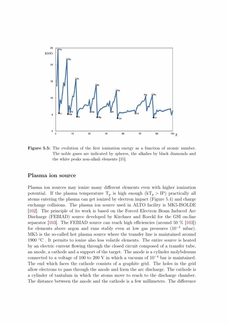
Figure 5.5: The evolution of the first ionization energy as a function of atomic number.The noble gases are indicated by spheres, the alkalies by black diamonds andthe white peaks non-alkali elements [35].

Plasma ion source

Plasma ion sources may ionize many different elements even with higher ionizationpotential. If the plasma temperature Tp is high enough (kTp > IP) practically allatoms entering the plasma can get ionized by electron impact (Figure 5.4) and chargeexchange collisions. The plasma ion source used in ALTO facility is MK5-ISOLDE[102]. The principle of its work is based on the Forced Electron Beam Induced ArcDischarge (FEBIAD) source developed by Kirchner and Roeckl for the GSI on-lineseparator [103]. The FEBIAD source can reach high efficiencies (around 50 % [103])for elements above argon and runs stably even at low gas pressures (10−5 mbar).MK5 is the so-called hot plasma source where the transfer line is maintained around1900 C . It permits to ionize also less volatile elements. The entire source is heatedby an electric current flowing through the closed circuit composed of a transfer tube,an anode, a cathode and a support of the target. The anode is a cylinder molybdenumconnected to a voltage of 100 to 200 V in which a vacuum of 10−4 bar is maintained.The end which faces the cathode consists of a graphite grid. The holes in the gridallow electrons to pass through the anode and form the arc discharge. The cathode isa cylinder of tantalum in which the atoms move to reach to the discharge chamber.The distance between the anode and the cathode is a few millimeters. The difference

in potential between the anode and cathode will remove electrons from the elements.At the output of the source the ions are subjected to a potential difference of 30 kVand transported to the mass separator.

Figure 5.6: Drawing of the MK5 ion source [102].

Laser ion source

The principle of the laser ion source is based on the resonant ionization method whichwas developed for resonance ionization spectroscopy (RIS) [104, 105]. The RIS methodis based on ionization by absorption of one or more photons (photoionzation) comingfrom laser beams. The absorption by an atom of one or more photon ejects an elec-tron from the electron cloud of the atom. In case of two steps ionization the first lightbeam is tuned to the frequency of the resonant transition of a given state (usually theelectronic ground state) to an intermediate state. The atom is then photoionized fromthis intermediate state with a second laser pulse. This method has two advantages.First of all, as the levels of the electrons vary for different elements it permits creationsof very pure radioactive beam of ions (high selectivity). This selective ionization ofatoms is due to the choice of the unique combination frequency laser to ionize theatoms of a selected item which prevents the ionization of other atoms. The secondadvantage is the ionization efficiency which is maximal if each atom in its ground stateexposed to the laser flux is ionized.

Figure 5.7: Schematic of different methods of ionization and the corresponding cross sec-tions (photo [35]).

Ionization schemes include two, three or more transitions (Figure 5.7) and are classifiedaccording to the nature of the last populated level before ionization:

• Ionization to the continuum:In the case of ionization to the continuum the last step of the ionization is non-resonant. The non-resonant cross-sections into the continuum are relatively small(σ = 10−17 − 10−18 cm2). The ionization efficiency depends strongly on the laserpower for the last transition. A strong non-tunable laser is used for this non-resonant step. The minimum energy of the beam of light required for ionizationis of the order of a few mJ/pulse. The ionization to the continuum is used whenthe autoionizing states are not known or too narrow.

• An autoionizing state (AIS):In the case of autoionization method, the ionization is resonant and the crosssection is higher than for the non-resonant ionization (σ = 10−15 − 10−16 cm2).An autoionizing state (AIS) is a two electron excitation above the atomic ion-ization potential Wi which decays in a radiationless transition into an ion andan electron. While one electron is ejected the other drops to the ground state orexcited state of the ion. Typical lifetimes of AIS are from 10−15 − 10−10 s. Allmany-electron atoms have autoionizing states but the knowledge of those states

is limited to few elements. The autoionizing states have very precise frequencyand require the use of lasers with high resolution.

• Transitions to a Rydberg state:The last type of ionization is ionization to Rydberg states [106, 107]. Usingthis ionization method high cross-sections can also be obtained (of the order ofσ = 10−14 cm2). However, to allow the ionization of the atom, the application ofa static electric field (approx. 10 kV/cm) is required to move by Stark effect theRydberg levels to the continuum [108, 109]. The necessity of a strong electricfield to induce the Stark effect makes this method difficult to implement.

5.4 The ALTO facility

The ALTO facility (Figure 5.8) can be decomposed into three main components: theelectron accelerator (LINAC), the target-ion-source unit and the mass separator (PAR-RNe).

Figure 5.8: The scheme of the ALTO facility.

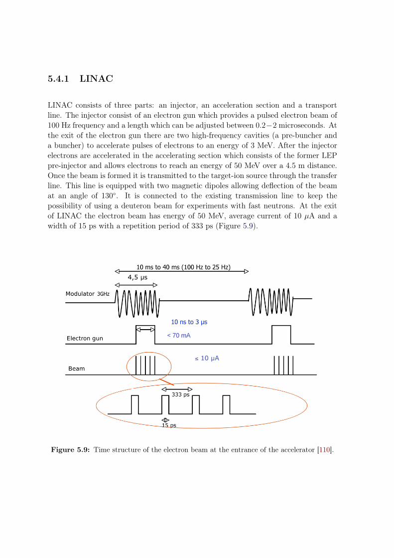
5.4.1 LINAC

LINAC consists of three parts: an injector, an acceleration section and a transportline. The injector consist of an electron gun which provides a pulsed electron beam of100 Hz frequency and a length which can be adjusted between 0.2−2 microseconds. Atthe exit of the electron gun there are two high-frequency cavities (a pre-buncher anda buncher) to accelerate pulses of electrons to an energy of 3 MeV. After the injectorelectrons are accelerated in the accelerating section which consists of the former LEPpre-injector and allows electrons to reach an energy of 50 MeV over a 4.5 m distance.Once the beam is formed it is transmitted to the target-ion source through the transferline. This line is equipped with two magnetic dipoles allowing deflection of the beamat an angle of 130. It is connected to the existing transmission line to keep thepossibility of using a deuteron beam for experiments with fast neutrons. At the exitof LINAC the electron beam has energy of 50 MeV, average current of 10 µA and awidth of 15 ps with a repetition period of 333 ps (Figure 5.9).

Figure 5.9: Time structure of the electron beam at the entrance of the accelerator [110].

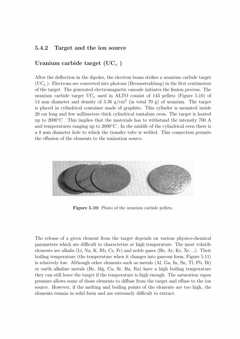
5.4.2 Target and the ion source

Uranium carbide target (UCx )

After the deflection in the dipoles, the electron beam strikes a uranium carbide target(UCx ). Electrons are converted into photons (Bremsstrahlung) in the first centimetersof the target. The generated electromagnetic cascade initiates the fission process. Theuranium carbide target UCx used in ALTO consist of 143 pellets (Figure 5.10) of14 mm diameter and density of 3.36 g/cm3 (in total 70 g) of uranium. The targetis placed in cylindrical container made of graphite. This cylinder is mounted inside20 cm long and few millimeters thick cylindrical tantalum oven. The target is heatedup to 2000C . This implies that the materials has to withstand the intensity 700 Aand temperatures ranging up to 2000C . In the middle of the cylindrical oven there isa 8 mm diameter hole to which the transfer tube is welded. This connection permitsthe effusion of the elements to the ionization source.

Figure 5.10: Photo of the uranium carbide pellets.

The release of a given element from the target depends on various physico-chemicalparameters which are difficult to characterize at high temperature. The most volatileelements are alkalis (Li, Na, K, Rb, Cs, Fr) and noble gases (He, Ar, Kr, Xe ...). Theirboiling temperature (the temperature when it changes into gaseous form, Figure 5.11)is relatively low. Although other elements such as metals (Al, Ga, In, Sn, Tl, Pb, Bi)or earth alkaline metals (Be, Mg, Ca, Sr, Ba, Ra) have a high boiling temperaturethey can still leave the target if the temperature is high enough. The saturation vaporpressure allows some of those elements to diffuse from the target and effuse to the ionsource. However, if the melting and boiling points of the elements are too high, theelements remain in solid form and are extremely difficult to extract.

Figure 5.11: The melting and the boiling point for different chemical elements.

5.4.3 The laser ion source at ALTO

Ionization scheme for gallium isotopes

In case of the ionization of gallium atoms one uses ionization to the continuum methodwhere two beams of laser are needed. The ionization scheme for gallium atoms, pre-sented in Figure 5.12, consists of two steps:

• the first transition is an excitation of the electron from the electronic groundstate 4s24p2P1/2 to the intermediate excited state 4s24d2D3/2. For this step theUV laser with a wavelength of 287.4 nm is used.

• the second step is the ionization from the 4s24d2D3/2 level to the continuum usinga green beam of 532 nm wavelength.

With the laser ion source the efficiency for the ionization of gallium atoms achieved atISOLDE (CERN) was 21% [100].

Figure 5.12: Two step ionizationscheme for gallium[35]. The maximumefficiency for the ion-ization of galliumatoms with the laserion source achievedat ISOLDE (CERN)was 21% [100].

Ionization of gallium atoms at ALTO

In order to insure maximum ionization of the gallium atoms in our experiment thenew laser ion source system was built. The schematic view of the system is presentedin Figure 5.13. It consisted of two lasers:

• the pump laser Edgewave Nd:Yag (model INNOSLAB IS2011-E). This laser pro-vides vertically polarized 532 nm beam with a pulse repetition rate of 10 kHzand a pulse duration of 10 ns. The maximum rated power of the laser is 100 W.

• the dye laser (commercial-type Lambda Physik model FL3002). The Lambda-Physik dye lasers can deliver wavelengths from 300 nm to 900 nm. To obtainthe wavelength of interest (UV light) a Rhodamine 6G dye was used. The dyelaser has an oscillator, a preamplifier and two amplifiers. The oscillator andthe preamplifier consist of a cell in which the dye flows at a high speed. Thisunit operates in two steps, the first is the oscillator (pumping the cell) thatgenerates the laser beam required wavelength, and the second, the preamplifierthat amplifies the beam.

Two laser beams are obtained in following procedure:

1. Inside the Nd:Yag laser, the cavity produces a light of a wavelength of 1064 nm.The frequency of this beam is doubled inside the laser with a nonlinear BBO(barium borate crystal BaB204) crystal to obtain at the exit a green laser beamof 532 nm. The beam coming out from the pump laser is split into two with abeam splitter (having 30% and 70% of the initial power for the first and secondbeam, respectively). The first beam of 532 nm is guided directly to the ionizationtube. Since the cross section for this transition is low (σ = 10−18 − 10−17 cm2)the power of the laser was relatively high (30 W). The transmission of the beamto the ionization tube was 67% , 20 W at the source.

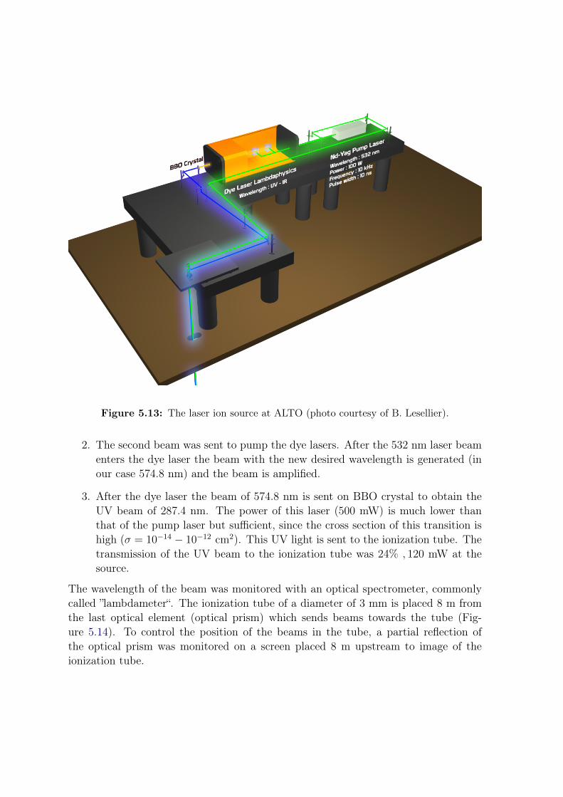
Figure 5.13: The laser ion source at ALTO (photo courtesy of B. Lesellier).

2. The second beam was sent to pump the dye lasers. After the 532 nm laser beamenters the dye laser the beam with the new desired wavelength is generated (inour case 574.8 nm) and the beam is amplified.

3. After the dye laser the beam of 574.8 nm is sent on BBO crystal to obtain theUV beam of 287.4 nm. The power of this laser (500 mW) is much lower thanthat of the pump laser but sufficient, since the cross section of this transition ishigh (σ = 10−14 − 10−12 cm2). This UV light is sent to the ionization tube. Thetransmission of the UV beam to the ionization tube was 24% , 120 mW at thesource.

The wavelength of the beam was monitored with an optical spectrometer, commonlycalled ”lambdameter“. The ionization tube of a diameter of 3 mm is placed 8 m fromthe last optical element (optical prism) which sends beams towards the tube (Fig-ure 5.14). To control the position of the beams in the tube, a partial reflection ofthe optical prism was monitored on a screen placed 8 m upstream to image of theionization tube.

electron beam

uranium carbide target

extracted ion beam

photofission

ionisation

8 m distance3 mm diameter

Isolde -type ion source

Figure 5.14: Schematic view of the ionization source (photo courtesy of B. Lesellier).

Performance of the laser ion source

The performance of the laser ion source was tested with a stable 69Ga beam duringa one week test run performed before the experiment to study 84Ga beta-decay (seeChapter 6). The number of ions was monitored by measuring the current with twoFaraday cups, one placed behind the mass separator and the second before the collec-tion point on the tape. The ionization of 69Ga with the laser was a factor of ten higherthan with the surface ionization (the measured current was 1 nA and 10 nA withoutand with the laser, respectively).

Figure 5.15 shows a part of the γ-ray spectrum measured with the surface ioniza-tion ion source (blue) compared to the spectrum measured in our experiment with thelaser ion source (red) for mass A = 84. The spectrum in blue was measured duringthe experiment performed in 2008 at ALTO [39, 49]. One can instantly notice a greatimprovement in the statistics and the purity of the spectrum achieved thanks to thelaser ion source, higher beam intensity (blue: 1 µA, red: 10 µA) and the lead shieldingof the mass separator to prevent the random coincidences of rubidium which was veryabundant in the previous experiment.

84Ge 2+→0+ 624 keV

84Ga→84GeT

1/2= 0.085(10) s

red: laser ionization ε~10%& 10 µA & improved shieldingblue: surface ionization ε~1%& 1 µA

84Se

84Ge

84Ge

83As

89-96Rb

94Rb83As94Rb

92-96Rb

Figure 5.15: Energy spectrum measured for mass 84 with surface ionization ion source andwit the newly developed at ALTO laser ion source.

5.4.4 Mass separator PARRNe

Ions affected by the 30 kV potential at the exit of the ion source travel to the massseparator (PARRNe). The mass separator is isolated from the target-ion source unitwith a 1.5 m thick concrete wall and the experimental room with a 20 cm thick concretewall. It shields from background radiation (γ’s) and neutrons coming from the targetor accumulated in the magnet. The beam has a good optical quality and is well focusedto optimize the transmission and the resolution of the mass separator. The ions areseparated in mass with a H-shaped electromagnetic dipole separator [111, 112]. It hasa homogeneous magnetic field B which is adjustable, a deflection angle of 65 and aradius of curvature ρ of 60 cm. The mass selection is proportional to the mass numberA of the nuclei and inversely proportional to the charge of the ion q · e (ρ · B =

√2·E·Mq·e

where M is the mass of the isotope). As most of the ions are of charge 1+, those aremass separated. The separation between two beams ∆x of masses m and m + ∆m isexpressed by the equality ∆x = D · ∆m

mwhere D = 1370 mm is the dispersion of the

magnet. As an example, the resolution of the separation of the masses 100 and 101 is13.7 mm [89].

Chapter 6

Experimental set-up

Contents6.1 Experimental details . . . . . . . . . . . . . . . . . . . . . . . . . 69

6.2 Detection system . . . . . . . . . . . . . . . . . . . . . . . . . . . 70

6.2.1 The tape system . . . . . . . . . . . . . . . . . . . . . . . . . . . 70

6.2.2 Electronics . . . . . . . . . . . . . . . . . . . . . . . . . . . . . . 72

6.2.3 Acquisition system . . . . . . . . . . . . . . . . . . . . . . . . . . 74

6.3 Performance of the detection set-up . . . . . . . . . . . . . . . 74

6.3.1 Germanium detectors . . . . . . . . . . . . . . . . . . . . . . . . 76

6.3.2 BGO shield . . . . . . . . . . . . . . . . . . . . . . . . . . . . . . 78

6.3.3 Veto detector . . . . . . . . . . . . . . . . . . . . . . . . . . . . . 81

6.1 Experimental details

The experiment dedicated to study β-decay of neutron-rich gallium isotopes was per-formed at ALTO in 2011. It was the test run of the facility dedicated to the safetymeasurements in the phase of the commissioning of ALTO. The fission fragments wereproduced with the photo-fission reaction induced by 50-MeV electron beam in a thickUCx PARRNe type target. It was the first experiment performed at ALTO whereelectron beam intensity was 10 µA which is the maximum electron intensity providedby the LINAC. The uranium carbide target was heated up to 2000 C to allow thediffusion of fission products. The elements diffused to the transfer tube where thegallium atoms were ionized with the selective laser ion source newly installed at theALTO facility. Those gallium ions were extracted with the 30 kV electric field andtraveled to the mass separator. The field in the PARRNe mass separator was set topass only the atomic mass 84 (to obtain desirable pure beam of 84Ga). At the laststage, those ions were implanted on aluminum-coated mylar tape.

Figure 6.1: Schematic view of the tape sta-tion and the detection system.Figure courtesy of G. Germogli.

6.2 Detection system

6.2.1 The tape system

The nuclei of interest were implanted into the aluminum-coated mylar tape. Thetape is rolled on two reels above the detection system. As it goes down it interceptsthe beam, extends a bit farther down and turns up again ending in the second reel(Figure 6.1). The system is kept under the same vacuum as the beam transport line.The implanted radioactive nuclei and their descendants undergo β-decay. In orderto obtain the clean spectrum (meaning not polluted by the γ-rays from the daughternuclei) the tape has to be moved in cycles so that the implantation position changesand the previous one in far enough (∼ 1.3m) to not to contribute as a backgroundradiation source. The average time required for one tape move is 2 s. The tapemovement was set and controlled with an automatic system which sends the signalto the acquisition system (“coding enable”) once the tape is stable, to allow for theacquisition.

Choice of the measurement cycles

The choice of the time of the cycle obviously depends on the half-life of the element ofinterest and the half-lives of the daughters, as well as precision required for the half-life determination. The number of nuclei present on the tape increases owing to theproduction rate and decreases owing to the radioactive decay (Eq. 4.1). The numberof parent nuclei decreases with time and the number of daughter nuclei increases as aresult of the decay of the parent and decreases as a result of its own decay (Eq. 4.7).The relative production of 84Ga on the tape (assuming that the neutron emissionprobability for gallium is 74(14) %[37]) and the descendants as a function of time isschematically presented in Figure 6.2.

Figure 6.2: Simulation of the activity of 84Ga and its descendants on the tape during thecycle of 4 s of “collection time“ and 1 s ”decay time“.

The collection time was chosen to last three seconds:

• to discriminate the half-lives of the peaks. This information permits us to knowthe origin of the γ-line. If the half-life of the chosen line is compatible withthe half-life of 84Ga (half-live of 84Ga 0.085(10) s [113]) one can believe this linebelongs to the β/β n-decay of this element.

• in order to obtain as much as possible γ − γ coincidences from 84Ga β-decay.As seen in Figure 6.2 the production of gallium saturates already after 1 s ofcollection. The 84Ga isotope is short lived and will decay during very short time(1 s). The longer the time when collecting ions the more decays and thus, themore γ − γ coincidence recorded by the detection system.

• to have the least contribution from the descendants possible. The short-lived84Ga β/β n-decays to 83,84Ge isotopes which then decay to arsenic. The longerthe collection time the more descendants are created and the more peaks appearon the spectra recorded with germanium detectors. In order to minimize thiscontribution on the spectrum the production of the daughter nuclei (productionthrough the decay of the mother) should not be higher than the one of the mothernuclei.

The time required for the decay of gallium (as seen in Figure 6.2) is only one second,and it was set to be the “decay time”.

6.2.2 Electronics

The schematic view of the electronic system is drawn in Figure 6.3.

• germanium detectors: The signal from the detector was first connected to thepreamplifier placed close to the crystal (to reduce the thermal noise and achievean optimum charge collection). From the preamplifier the signal was sent tothe Linear Amplifier where it was amplified and its shape was formed into semi-Gaussian shape. The decay part of the signal is determined by the feedbackcircuit of the preamlifier. To avoid so called undershoots (which is the differen-tiation of exponential tail from the preamplifier), which may cause an amplitudedefect in case if the second signal arives just after the first one, the pole-zerocancelation circuit was used. The time signal from the detector was sent first tothe Fast Timing Amplifier (FTA). It provided voltage pulses which amplitudesare proportional to the incident amplitudes. This signal was then changed intoa logical signal by Constant Fraction Discriminator (CFD). The rising edge ofthis logic signal was used to trigger the acquisition of the energy channel. Sincethe Linear Amplifier process is much slower than the FTA or the CFD, in orderto fulfill the condition of coincidence, the signal was delayed before entering tothe acquisition card.

• BGO detector: Each of 10 crystals was connected to a photomultiplier. Thesignal from each PMT was sent to the Dual Gate Generator (DGG) where thethreshold (the minimum energy of the incident gamma) for each of them wasset independently. The signal from BGO shield was recorded as “marker“ byacquisition card if there was an event detected in one of the crystals. Thisevent was used to build a coincidence (when two signals, one from BGO and thesecond from germanium detector occur in short time interval) with the GFOC24germanium detector.

• plastic detector 4πβ: The signal from the plastic detector 4πβ was sent to theConstant Fraction Discriminator and then directly to acquisition card. Thislogic signal was used in the analysis process to built the coincidences with thegermanium detector.

• Veto: The time signal from the plastic detector Veto was amplified with theTFA and then double with Fan In/OUT module. One of the signals traveledto the Dual Gate Generator and from there to acquisition card (as ”marker“for GV1 germanium detector), the second was used as a timing signal to buildcoincidences with germanium detectors.

Figure 6.3: Schematic view of the electronic system.

6.2.3 Acquisition system

The analog signals from the electronics were transmitted to the acquisition cardCOMET-6x (Coding Marked Time) where they were converted into numeric format.The card has 6 channels, each channel has three inputs: one for energy signal, thesecond for time signal and the third input for the marker. The energy signal is codedin 15 bits, the time 47 bits and the marker is a logic NIM 1-bit signal. The COMETsystem is a trigger-less system. Each detector (plastic scintillator, germanium detec-tor) is considered as an independent source for which the physical signal associatedwith an absolute time is coded. The time accuracy is 400 ps. The COMET cardcan encode up to 20000 events per second per channel (which is well above the countrate usually observed at ALTO when studying very neutron-rich species). During theexperiment the CODEN (Coding Enable) signal was used. It is a TTL signal sent bythe tape station system which inhibits the coding while the tape is moving (0 V codinginhibited, 5 V coding enable). Each cycle the absolute COMET time is reset to zero.Only the radiation from the cycles sent to the tape station system are measured. Thedata are transmitted and stored on the server. The data can be monitored on-lineduring the experiment with the computer program “cvisu”. This program creates theenergy spectra of 15 bits and time spectra of 47 bits.

6.3 Performance of the detection set-up

The detection system is presented in Figure. 6.4:

• two germanium detectors GV1 and GFOC24 (the energy resolution of 2.6 keVand 2.3 keV at 1 MeV, respectively) cooled down with liquid nitrogen usingautomatic cooling system,

• cylindrical shape 4πβ plastic detector, providing an angular acceptance of 4πsr,was used to detect β particle from β−decay,

• to reject the background radiation (Compton contiuum), the detector GFOC24was shielded with BGO shield (which is the prototype for the ORGAM2 projectunder construction in IPN Orsay). The BGO shield was used for the rejectionof the Compton scattered γ-rays.

• plastic detector Veto was placed in front of the second germanium GV1. Thisdetector was used to reject the electron continuum produced in the germaniumcrystal.

Figure 6.4: Top: Picture of the detection system. Bottom: Schematic view of the detectionsystem.

6.3.1 Germanium detectors

Efficiency

The efficiency of germanium detectors was measured with calibrated 152Eu, 137Cs and60Co sources placed at the position of the collection point. The total efficiency of ourdetection system and a fit function with several adjustable parameters are plotted inFigure 6.5. The efficiency of the detection system was 2% at 1 MeV.

Figure 6.5: Efficiency of the germanium detectors measured with 152Eu, 137Cs and 60Cosources.

Energy calibration and resolution

The energy calibration for germanium detectors was performed using the calibrated152Eu source and, additionally, for better precision at the higher energy, the tabulatedpeaks of 84Ge [114] were used. As a fit for the energy calibration, second polyno-mial was used. The precision of the energy calibration is plotted in Figure 6.6. Theresolution of the germanium detectors system as a function of energy is presented inFigure 6.7 for detectors GFOC24 and GV1. The energy resolution of the detectionsystem was 2.8 keV at 1 MeV.The timing resolution for β-γ coincidences, calculated from the full width at half maximum, was 20 ns and 40 ns for GFOC24 and GV1 at 1 MeV, respectively (for moredetails see Chapter 7, Figure 7.1).

Channel0 500 1000 1500 2000 2500 3000 3500

Ekn

own-

Eca

lib [k

eV] G

FO

C24

-0.4

-0.2

0

0.2

0.4

0.6

0.8

1

Channel0 500 1000 1500 2000 2500 3000 3500

Ekn

own-

Eca

lib [k

eV] G

V1

-0.8

-0.6

-0.4

-0.2

0

0.2

0.4

0.6

Figure 6.6: The precision plot of the energy calibration for GFOC24, GV1 germaniumdetectors. The energy precision is 0.4 keV and 0.5 keV for GFOC24 and GV1,respectively.

Energy [keV]0 500 1000 1500 2000 2500 3000 3500

sigm

a

0.6

0.8

1

1.2

1.4

1.6

1.8

2

2.2

/ ndf 2χ 78.91 / 32

p0 0.01158± 0.4988

p1 4.726e-05± 0.0009629

/ ndf 2χ 78.91 / 32

p0 0.01158± 0.4988

p1 4.726e-05± 0.0009629

Figure 6.7: Resolution of the germanium detectors as a function of the energy. The resolu-tion is measured with the spectrum from 84Ga β-decay.

6.3.2 BGO shield

Of the various ways γ-rays can interact in matter photoelectric absorption, pair pro-duction, and Compton scattering are the most significant. Photoelectric absorptionpredominates for γ-rays up to several hundred keV, pair production predominates forenergy above 5− 10 MeV, and Compton scattering is the most probable process overthe range of energies between those extremes [115]. Partial absorption of γ-ray energydue to Compton scattering results in continous background (Compton continuum)which extends up to its maximum called Compton edge.

In our experiment bismuth germanate (B4G3O12) scintillator detector was used asa shielding against Compton scattered γ-radiation. It consisted of five high-efficiencycrystals mounted in pentahedral shaped carbon cell (Figure 6.8). Each of the crystalswas connected to two photomultipliers. The signal from each photomultiplier was sentto the input of the Constant Fraction Discriminator. The threshold in the ConstantFraction Discriminator was adjusted for each photomultiplier, with 60Co source placedin front of the germanium detector, in order to obtain the same counting rate in eachof them.

Figure 6.8: Left top: BGO crystals. Right top: two photomultipliers connected to BGOcrystal. Bottom: the pentahedral carbon cell. Courtesy of T. Zerguerras.

The performance of the shield (the so-called rejection factor) was tested with thecalibrated 60Co source, with the source placed 2 cm in front of detector. The photo-peak to total ratio, the number of counts in the two cobalt peaks compared to thenumber of counts in the spectrum with and without the Compton rejection give thequantitative factor for the rejection. The results of the measurement is presentedin Figure 6.9. Without the Compton rejection the ratio peak/total = 0.269. Whenwe included BGO shield the ratio was 0.414 what indicates that a great part of thebackground was rejected. The suppression factor of the BGO shield as a function ofincident γ energy is plotted in Figure 6.10. The suppression factor is the ratio betweencounts in the unsuppressed and suppressed spectra. The factor was on average 2,except for the high energy γ-rays going forward. Since the shield was placed aroundthe germanium crystal forward and backward angles were not covered, thus highlyenergetic γ-rays are not rejected.

No rejection:

Nphotopeaks/Ntot= 0.269

AC rejection:

Nphotopeaks/Ntot= 0.414

10mm 60Co

20mm

Ge

Figure 6.9: Measured γ-ray spectrum of 60Co with and without Compton suppression. Fig-ure courtesy of T. Zerguerras.

Figure 6.10: The suppression factor of the BGO shield as a function of incident γ-ray energy.

6.3.3 Veto detector

The primary electrons, β− particles or electrons produced through various mecha-nisms of interaction of γ-radiation with matter, continuously lose their kinetic energyin the detector absorber material. Large deviation of their path are possible becauseits mass is equal to that of the orbital electron with which it is interacting and muchlarger fraction of its energy can be lost in a single encounter [115]. Electrons maylose their energy through radiative processes. The major component of such losses isBremsstrahlung, which is an electromagnetic radiation produced by the interaction offast electrons with the Coulomb field of a nucleus in the absorbing material and canbe emitted from any position along the electron track. The fraction lost by this pro-cess increases sharply with electrons energy and becomes dominant for electrons withenergy over few MeV [115]. The electron energy deposition through Bremsstrahlungin the germanium detector may extend to the maximum energy of the β-particle, butsignificant yields can be seen as a continuous low-energy background. In our experi-ment, the electrons interacting in the detectors originate from the β-decay of the ionsimplanted on the tape (in case of 84Ga decay Qβ = 13690 keV [116]) or from the cosmicradiation in the detector (typically ionization muons). Because of close geometry ofthe detection system the backscattered electrons can also bring the contribution to theenergy spectrum. The Bremsstrahlung contribution cannot be simply substracted asa background and its inclusion may lead to errors in measurements of peak areas. Inorder to minimize this background the plastic Veto detector (Figure 6.11) was placedin front of germanium detector GV1 to serve as a marker for the events created by theelectrons.

Figure 6.11: Left: Picture of the Veto plastic detector. Right: Veto detector installed infront on the germanium GV1 detector. Courtesy of S. Ancelin.

The result of the background subtraction with the Veto plastic detector in presentedin the coincidence spectra in Figure 6.12. The black line is the β − γ spectrum of the

detector GFOC24 and the 4πβ plastic detector. With the β−γ coincidence one ensuresto have in the spectrum the γ-lines which belong to the β-decay. The blue line presentsthe result of β-γ-BGO anticoincidence where the coincidence with the BGO shield isincluded (one can clearly see the disappearance of the Compton-scattering part ofthe spectrum). However, even after Compton rejection the low energy background isstill present. It most probably originates from Bremsstrahlung process. In order tofind out what is the origin of this background the third spectrum was built with thecoincidence with the Veto detector (red line). In this case the accepted events wherethose that occured in detector GFOC24 in coincidence with 4πβ and anticoincidencewith BGO shield if at the same time the electron was detected on the other side of theinteraction point: in the Veto plastic detector. Obviously, since the Veto detector wasplaced in front of GV1 detector, the acceptance angle was small and the statistics onthe spectrum is low. The optimal position would be to mount it in front of GFOC24and use in anti-coincidence procedure. Nevertheless, the data analysis described abovehelped us to understand the origin of this background. The lower-energy continuousbackground, greately minimized on the red spectrum, as suspected comes from theelectron contribution in the germanium detector.

Sun Apr 1 16:57:35 2012 Energy (keV)100 200 300 400 500 600 700

coun

t/keV

0200400600800

100012001400160018002000

Compton

β−γ

β−γ BGO

242keV

peak/bkg. = 2

peak/bkg. = 4

β−γ BGO veto

peak/bkg. = 1.5

electron contribution

GV1 GFOC24

Figure 6.12: The β − γ coincidence spectra with background rejection. Thepeak/background ratios at 242 keV: without Compton rejection 1.5, withCompton rejection 2, including the coincidence with the Veto detector 4.

Chapter 7

Data analysis and results

Contents7.1 Analysis procedure . . . . . . . . . . . . . . . . . . . . . . . . . 83

7.1.1 Time spectra . . . . . . . . . . . . . . . . . . . . . . . . . . . . . 84

7.1.2 Determination of the half-life . . . . . . . . . . . . . . . . . . . . 85

7.1.3 The γ-γ coincidences . . . . . . . . . . . . . . . . . . . . . . . . . 88

7.2 Experimental results . . . . . . . . . . . . . . . . . . . . . . . . 90

7.2.1 The β-gated energy spectrum . . . . . . . . . . . . . . . . . . . . 90

7.2.2 Results for 84Ge . . . . . . . . . . . . . . . . . . . . . . . . . . . 90

7.2.3 Results for 83Ge . . . . . . . . . . . . . . . . . . . . . . . . . . . 95

7.2.4 Results for 84As . . . . . . . . . . . . . . . . . . . . . . . . . . . . 98

7.3 Spin assignment . . . . . . . . . . . . . . . . . . . . . . . . . . . 104

7.1 Analysis procedure

The data generated by COMET-Narval acquisition are registered, event by event, ina format specific for this acquitistion system [117]. Since we decided to perform theanalysis with software ROOT, the data generated by the COMET-Narval acquisitionwere converted with NarvalToRoot “Event Builder“ [49] to a format (ROOT) suit-able for their further treatment. The events were stored in the ROOT trees (TTree),each divided into several branches containing specific information (e.g. energy, time,marker). The type of each branch was declared depending on the information it con-tained. To optimize the size of the data each branch was compressed independently,this conversion reduced the volume of the data by at least one third compared to theCOMET-Narval format where the data are not compressed. The time required to re-read the data is also greatly reduced, especially when one wants to re-read only specificbranches. The branches could be read independently from each other, depending onthe needs.

Analysis of the data requires the reconstruction of the correlations between differ-ent events, e.g. in case of β-decay considered events are β particle and γ-ray. Theacquisition in the COMET system is triggerless which means that each detected eventis saved on the disk with a time stamp (an integer stored in 47 bits) where ”time”(in β-decay experiment with measurement cycles) is relative to the last coded signaland each signal resets the clock. The ROOT tree contains the raw data with thetime stamp conversted into double precision float (64 bits) and the events are listedin chronological order. The time of the event is used to build so-called “coincidences“which associate events in time when the time window for those events is less than atime window (”coincidence window”) specified by the user.

In the following subsections, the procedure of the data analysis is described. At first,the β-γ coincidences time spectra are presented and the time resolution of the ger-manium detectors is calculated. In the second part, we describe the procedure fordetermination of the half-life of γ-lines. Finally, the example of the analysis of γ-γcoincidences is shown.

7.1.1 Time spectra

It is essential to build a β-gated energy spectrum to assure that the γ-lines in thespectrum come from the β-decay. The coincidence of γ-ray detected in germaniumdetector and β particle seen by plastic detector allow us to built that kind of energyspectra. In order to obtain a proper energy spectrum one needs to investigate the timespectra for the coincidences. The plastic detectors are much faster than the germaniumdetector, thus in principle, one expects to see the γ events in the germanium after theβ particle as a trigger detected in the plastic. The time spectrum is the difference intime between those two events (β and γ), or in other words if the β detector is a triggerand its time is set as a start zero time then the time distribution follows the time ofthe γ-ray detected after β-particle. To build the coincidence events the “coincidencewindow“ was chosen to be 500 ns. The distribution of β-γ coincidence events, for eachenergy of γ, in time is presented in Figure 7.1. Once gating on the chosen energy (inFigure 7.1 the gate is set on 1000 keV) one obtains the time distribution (right sideof the figure). One can see the steep slope on the left side of the peak and the tail ofthe right side. This tail is an electronic effect coming most probably from badly setConstant Fraction Discriminator treshold and should not be considered for the furtheranalysis. The time resolution for β-γ coincidence calculated from the full width athalf maximum, was 20 ns and 40 ns for GFOC24 and GV1 at 1 MeV, respectively. Tobuild the β-gated γ-spectrum (presented in Figure 7.6) or for β-γ-γ events (Figure 7.4)those time gates were used.

GFOC 24

GV1

Figure 7.1: Time distributions of β−γ coincidence events for the GFOC24 detector (upper)and the GV1 detector (lower plot).

7.1.2 Determination of the half-life

The ”time-energy” matrix represents the energy as a function of time in the mea-surement cycle. To build this matrix the contribution of all channels of germaniumdetectors is summed. The time-energy matrix allows to monitor the activity of γ-linesover a period of time. Using this data one is able to discriminate the half-life of theγ-line of interest and assign it to the proper decaying element.

The example of the determination of half-life for line at 624 keV (2+ → 0+ transitionin 84Ge) is presented in Figure 7.3. The time-energy matrix was analyzed in partialtime of 20 ns. Each 20 ns the energy spectrum was built, the gaussian peaks and thepolynomial functions were used for fitting both to the peak and the background. Theresult of the integration of the peak was used to built the activity spectrum in time(right top in Figure 7.3). In the final step, the half-life was determined from the fit ofthe growing and decaying parts of the curve (see Figure 7.2).

Figure 7.2: Example of thedetermination ofthe half-life. Twofunction were fit:one to the grow-ing part and thesecond to the de-caying part.

If we consider the decay of the mother to the daughter the following equations hold:

Acoll = P · (1− e−λtcoll) , (7.1)

Adec = P · (1− e−λtcoll)e−λtdec , (7.2)

where Acoll, Adec are the activities during the collection and the decay time, P is theproduction of the mother nucleus and λ = ln2/T1/2 contains the half-life of interest.The times are chosen to be 0− 4 s collection and 1 s for the decay.If one needs to consider the decay of the second generation the half-life will be obtainedfrom:

Acoll = P · (1− e−λ1tcoll) + P · λ2

λ2 − λ1

(e−λ2tcoll − e−λ1tcoll) (7.3)

Adec = P · λ2

λ2 − λ1

[λ2(1− e−λ1tcoll)e−λ1tdec − λ1(1− e−λ2tcoll)e−λ2tdec

](7.4)

where the index 1 describes the mother and the index 2 the daughter nucleus.

As 624 keV is the γ-line from (2+ → 0+) transition in 84Ge, Eq. 7.1 and Eq.7.2 werefit to determine properly the half-life. The obtained results 0.097(17) s is consistentwith the tabulated value 0.085(10) s [113], thus, proving that the line comes from thedecay of 84Ga.

20 ns 20 ns 20 ns 20 ns

20 ns 20 ns 20 ns 20 ns

20 ns

20 ns

20 ns

20 ns 20 ns 20 ns 20 ns

20 ns 20 ns 20 ns

20 ns 20 ns 20 ns

20 ns 20 ns 20 ns

Energy [600-660 keV]

coun

ts/0

.2ke

V

Figure 7.3: Procedure for the determination of the half-life. Left top: gaussian fit on theγ-line of interest, right top: a result of the time distribution from the fittingprocedure, bottom: fitting of the peak and the background in different timeperiods.

7.1.3 The γ-γ coincidences

The “energy-energy” matrix contains the triple coincidence of the β-γ-γ events in thespecified “coincidence window”. It allows us to seach for the γ-γ coincidences in theβ-decay which would correspond to the γ cascade in the excited states of the nucleusof interest. The matrix in presented in Figure 7.4. Except for the clear points fromthe γ coincidences one can also see oblique line from the backscattered γ-rays (due toa very close detection geometry).

Figure 7.4: The γ-γ coincidence energy matrix.

With the energy-energy matrix one can search for the γ-γ coincidences. The procedureis as follows: after choosing a peak of interest and subtracting the background fromthe right and left side of the peak and correcting from the factor of the number ofchannels one obtains the coincidence spectrum. To confirm the coincidence it is im-portant to gate on the γ-line seen in the coincidence to check if the coincidence reallyexists. The example of the coincidences with line at 624 keV (2+ → 0+ transition in84Ge) is shown in Figure 7.5. One can clearly see three lines: at 765 keV, 1605 keV and2878 keV in coincidence with 624 keV. The concidences are confirmed while looking atgate on those three γ-lines: the peak at 624 keV is well visible.

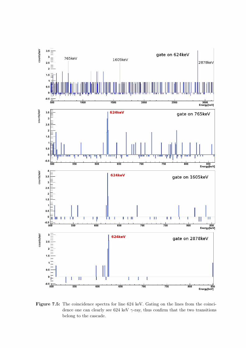
Figure 7.5: The coincidence spectra for line 624 keV. Gating on the lines from the coinci-dence one can clearly see 624 keV γ-ray, thus confirm that the two transitionsbelong to the cascade.

7.2 Experimental results

7.2.1 The β-gated energy spectrum

The β-gated γ-spectrum measured during three-day experiment is presented in Fig-ure 7.6. One can see the peaks belonging to 83,84Ge,83,84As and 84,83Se. There arealso γ-lines belonging to the neutron-rich Rb isotopes with mass ranging from 89 to96. The Rb isotopes are strongly favored in both the fission process and the ioniza-tion mechanism. For the ionization of gallium atoms the laser ion source was used,however, since the transfer tube is a W ionizer heated up to 2000 C which selectivelyionizes alkalies and also elements with particularly low first ionization potentials (seeFigure 5.5). The Rb isotopes were stopped within the separator chamber which wasadditionaly shielded with lead blicks. However, due to their high activity some ofthe γ-lines appear as random coincidences with β events. Despite this experimentaldifficulty the γ-lines characterizing the activity of nuclei of interest are clearly visibleproving that 84Ga was successfully ionized with the laser ion source and collected onthe tape.

7.2.2 Results for 84Ge

Thanks to higher electron beam intensity (10µA) and a laser ion source we were able toincrease the statistics. A new shielding around the focal plane of the magnet allowedus to have less contaminants from the Rb isotopes. We were able to discriminate thehalf-lives through γ-lines present in our spectrum and obtain γ−γ coicidence spectra.The population of the excited states of 84Ge through the β-decay of 84Ga allowedus to improve the level scheme of 84Ge. The first results from the β-decay studiesof 84Ga were observed at ISOLDE-CERN. The two short-lived elements with γ-lines:one at 624.3(7) keV and the other at 1046.1(7) keV [38, 39] were seen and assignedas belonging to the level scheme of 84Ge: as 2+

1 and 4+1 excited states. This result,

however, was not confirmed by Winger [37] who placed the 4+1 state at 1389.0(10) keV

and the γ-ray transition of 765.1(8) keV in coincidence with 623.9(6) keV.

The results of the half-life determination for four γ-rays assigned to the β-decay of84Ga are presented in Figure 7.7. Their determined half-lives: 0.097(17) s, 0.107(93) s,0.159(100)s, 0.086(29)s are all consistent with the half-life of 84Ga T1/2 = 0.085(10) s [113].From the coincidence spectra (presented in Figure 7.5) we were able to confirm theexistence of the state at 1389.1 keV and the coincidence with γ-ray of energy 623.9 keV,as well as improve the level scheme by adding two new coincidences (623.9 keV with1603.9 keV and 2878 keV) and the transitions to the ground state.

Due to the low statistics in the peaks at 1389 keV and 2878 keV, the determination of

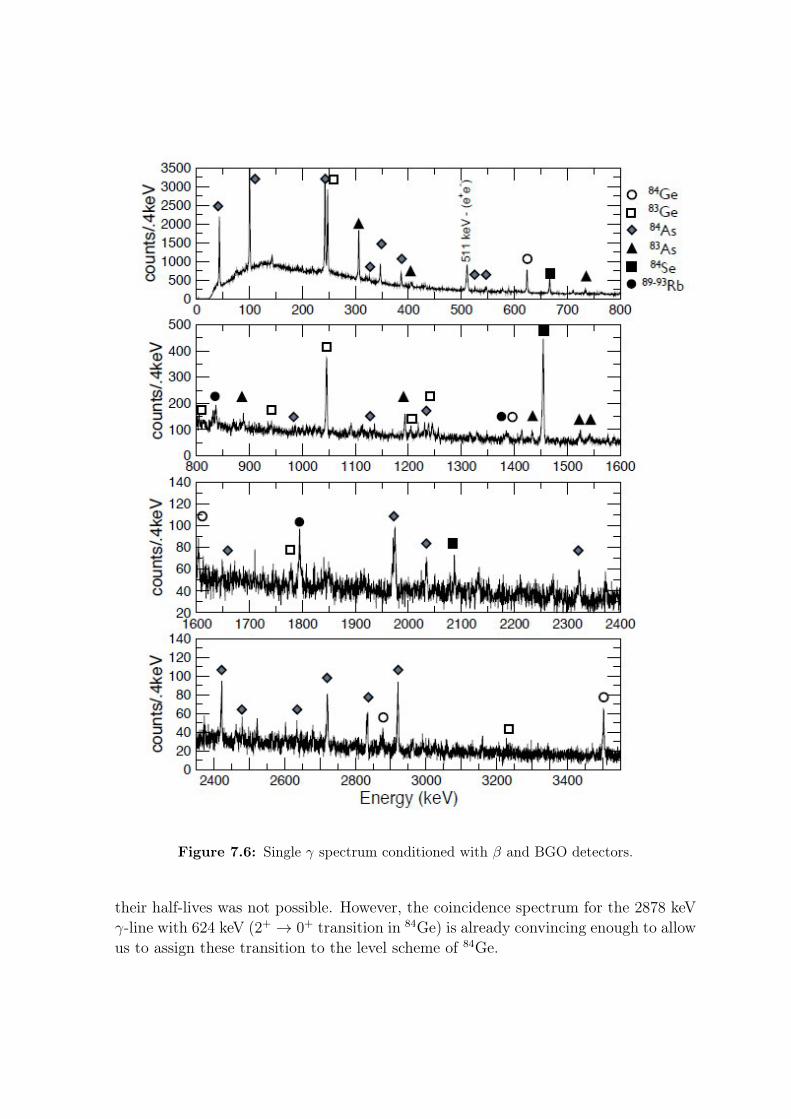
Figure 7.6: Single γ spectrum conditioned with β and BGO detectors.

their half-lives was not possible. However, the coincidence spectrum for the 2878 keVγ-line with 624 keV (2+ → 0+ transition in 84Ge) is already convincing enough to allowus to assign these transition to the level scheme of 84Ge.

Figure 7.7: The results of the half-life (in seconds) determination for the lines of 84Ge.

Table 7.1: The final list of γ-lines observed in the β-decay of 84Ga assigned to the de-excitation from the excited states of 84Ge. The list contains the energy of theγ-ray, the intensity as relative to the most intense γ-ray, the energy of the excitedlevel and the calculated half-life. The γ-ray with asterix to be confirmed.

Energy [keV] Relative intensity [%] Level [keV] Half-life [s]624.2(2) 100(5) 624.2(2) 0.097(17)765.1(3) 15(4) 1389.3(4) 0.107(93)*1389.3(4) 9(5) 1389.3(4)1603.9(2) 16(4) 2228.1(3) 0.159(100)2878.1(6) 21(7) 3502.3(6)3502(1) 50(7) 3502.3(6) 0.086(29)

To ensure the possibility of the transition at 1389 keV in 84Ge we performed carefullanalysis of the γ-peak 1389 keV. The zoom on the β-gated energy spectrum in theregion of the peak is presented in Figure 7.8. As one can see, the peak of interest issmall and located close to another peak at 1385 keV. The number of counts in peakswas estimated: 74(30) counts in the peak at 1385 keV and 28(9) counts in the peak at1389 keV (see Table 7.2).

Figure 7.8: Single β gated energy spec-trum zoomed to show theregion of interest (1370 −1400 keV) and the peak at1389 keV.

Table 7.2: Contribution of the activities of rubidium isotopes in peaks at 1385 keV and1389 keV.

Energypeak Counts Element T1/2 s Energy Intensity % Counts[keV] in peak [116] [keV] [116]

1385 74(30)92Rb 4.49(2) 1384.6(3) 3.6(7) 2(1)93Rb 5.84(2) 1385.21(8) 6.6(3) 74(32)

1389 28(9)91Rb 58.5(4) 1388.13(44) 0.22(3) 3(1)93Rb 5.84(2) 1388.7(6) 0.26(6) 1(1)

The peak at 1385 keV was identified as random coincidence γ-line from 93Rb iso-tope with half-life of 5.84(2) s [116]. This isotope has also very weak transition at1388.7(6) keV (intensity of 0.26(6)%). The estimation of the contribution from rubid-ium isotopes in those two peaks was done starting from the analysis of the biggestpeaks found in the spectrum. 93Rb has the strongest line at 432.61(2) keV (20.2(10)%

[116]) and the second strongest at 986.05(6) keV (7.9(4)%). We used those lines to es-timate the total activity of this isotope and further the contribution in the two peaks:1385.21(8) keV and 1388.7(6) keV. This contribution was found to be 74(32) countsand 1(1) counts, in those two peaks respectively (see Table 7.2).

Figure 7.9: The result-ing levelschemeof 84Ge.In black al-ready known[37, 38, 39],in red newlydiscoveredtransitions,the dottedtransition:tentativeassignmet. 32

84Ge52

3184Ga53

0+ 0.0

2+ 624.2H2L

H4+L 1389.3H4L

2228.1H3L

3502.3H6L

H0-L

624.

2H2L

@100

H5LD

765.

1H3L

@15H4L

D13

89.3

H4L@9H

5LD1603

.9H2L

@16H4D

L2878

.1H6L

@21H7L

D35

02H1L

@50H7L

D

92Rb (half-life of 4.49(2) s [116]) has line at 1384.6(3) keV with intensity of 3.6(7)%.The same procedure was done for this isotope starting from its strongest transitions:γ-lines of energy 814.98(3) keV (33(2)% intensity [116]) and 569.8(1) keV (5.6(3)%

intensity [116]) to estimate the total activity. Then the contribution of 92Rb in thepeak of interest at 1384.6(3) keV was calculated to be 2(1) counts. Third strongest γ-line of 91Rb was identified at 439.15(3) keV (2.09(10)% intensity [116]), using this linewe estimated the number of counts of this isotopes at the energy of 1388.13(24) keV(0.22(3)%) to be 3(1) counts.

The peak at 1385 keV was identified as 93Rb. Even summing the possible maximumactivities of 91Rb and 93Rb in the peak at 1389 keV (6 counts) there is still contributionfrom the other element (22 counts) which we assign as the transition in 84Ge. The finallevel scheme is presented in Figure 7.9 and the list of γ-lines, their relative intensitiesand half-lives are listed in Table 7.1.

7.2.3 Results for 83Ge

Up to now, only few transitions were assigned to the level scheme of the neutron-rich 83Ge. The low-lying excited states of 83Ge were populated in (d, p) reaction with82Ge beam at the Holifield Radioactive Ion Beam Facility (HRIBF) at Oak Ridge Na-tional Laboratory (ORNL) [47, 44], and with the β-decay of 83Ga performed at IPNOrsay [48, 49] and at HRIBF [37] (β-decay of 83Ga, β n-decay of 84Ga).

In our experiment we populated the excited states of 83Ge with β n-decay of 84Ga. Theresults of the discrimination of half-lives of few γ-lines are presented in Figure 7.10.

Figure 7.10: The results of the half-life (in seconds) determination for the lines of 83Ge.

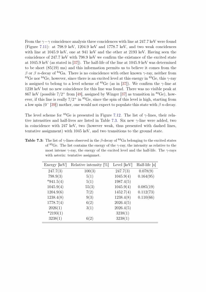
From the γ−γ coincidence analysis three concidences with line at 247.7 keV were found(Figure 7.11): at 798.9 keV, 1204.9 keV and 1778.7 keV, and two weak concidenceswith line at 1045.9 keV, one at 941 keV and the other at 2193 keV. Having seen thecoincidence of 247.7 keV with 798.9 keV we confirm the existance of the excited stateat 1045.9 keV (as stated in [37]). The half-life of the line at 1045.9 keV was determinedto be short (85(19) ms) and this information permits us to believe it comes from theβ or β n-decay of 84Ga. There is no coincidence with other known γ-ray, neither from83Ge nor 84Ge, however, since there is an excited level at this energy in 83Ge, this γ-rayis assigned to belong to a level scheme of 83Ge (as in [37]). We confirm the γ-line at1238 keV but no new coincidence for this line was found. There was no visible peak at867 keV (possible 7/2+ from [48], assigned by Winger [37] as transition in 82Ge), how-ever, if this line is really 7/2+ in 83Ge, since the spin of this level is high, starting froma low spin (0− [39]) mother, one would not expect to populate this state with β n-decay.

The level scheme for 83Ge is presented in Figure 7.12. The list of γ-lines, their rela-tive intensities and half-lives are listed in Table 7.3. Six new γ-line were added, twoin coincidence with 247 keV, two (however weak, thus presented with dashed lines,tentative assignment) with 1045 keV, and two transitions to the ground state.

Table 7.3: The list of γ-lines observed in the β-decay of 84Ga belonging to the excited statesof 83Ge. The list contains the energy of the γ-ray, the intensity as relative to themost intense γ-ray, the energy of the excited level and the half-life. The γ-rayswith asterix: tentative assignmet.

Energy [keV] Relative intensity [%] Level [keV] Half-life [s]247.7(3) 100(3) 247.7(3) 0.078(9)798.9(3) 5(1) 1045.9(4) 0.164(95)*941.5(4) 5(1) 1987.4(5)1045.9(4) 55(3) 1045.9(4) 0.085(19)1204.9(6) 7(2) 1452.7(4) 0.112(73)1238.4(8) 9(3) 1238.4(8) 0.110(66)1778.7(4) 6(2) 2026.4(5)2026(1) 3(1) 2026.4(5)*2193(1) 3238(1)3238(1) 6(2) 3238(1)

Figure 7.11: Top: The coincidence spectra for γ-line at 247 keV. Gating on the lines fromthe coincidence one can clearly see 247 keV γ-ray, thus confirm that the threetransitions belong to the cascade. Bottom: The coincidence spectra for γ-lineat 1045 keV.

3283Ge51

3184Ga53

Pn=74H14L%

52+ 0.0

12+ 247.7H3L

H72+L 867.4H5L1045.9H4L

H32+,52+L 1238.4H8L1452.7H4L

1987.4H5L2026.4H5L

3238H1L

H0-L

247.

7H3L

@100

H3LD

867.

4H5L

798.

9H3L

@5H1LD

1045

.9H4L

@54.9

H2.8LD

1238

.4H8L

@9H3LD

1204

.9H6L

@7H2LD

941.

5H4L

@5H1LD

1778

.7H4L

@6H2LD

2026

H1L@3H

1LD21

93H1L

3238

H1L@6H

2LD

Figure 7.12: The resulting level scheme of 83Ge. In black already known [37, 47, 44, 48], inred newly discovered transitions. The transition in blue was proposed by [48]but not confirmed yet. The level at 867 keV was not populated in this exper-iment. The two γ-lines drawn with the dotted lines (941 keV and 2193 keV),to be confirmed. The neutron emission probability from [37].

7.2.4 Results for 84As

The latest updated level scheme of 84As was presented by Tastet in thesis [35]. Heconfirmed already known γ-transitions at 42.7 keV, 100 keV, 242 keV, 386 keV and608 keV [51, 52, 49], added two γ-lines, one at 346.5 keV the other at 794 keV, bothin coincidence with 242 keV, and made spin assignement for low-lying states.

We confirmed the level scheme proposed by Tastet (except the line at 794 keV) andextend the scheme of excitation levels in 84As. The results for the discrimination ofthe half-life of the γ-lines are presented in Figure 7.13 and Figure 7.14. Many newcoincidences of γ-rays at 42.7 keV, 100 keV and 242 keV were found (Figure 7.15).

The final level scheme is presented in Figure 7.16. The list of γ-lines can be found inTable 7.4. Two new transitions to the ground state were assigned at 464.6 keV and589.9 keV, however, since the statistics for those peaks was poor, both of the weredrawn with the dashed lines (tentative assignement).

Figure 7.13: The results of the half-life (in seconds) determination for the lines of 84As.

Figure 7.14: The results of the half-life (in seconds) determination for the lines of 84As.

Figure 7.15: Top: the coincidence spectrum for γ-line at 43 keV, middle: the coincidencespectrum for γ-line at 100 keV, bottom: the coincidence spectrum for γ-lineat 242 keV.

3384As51

H3-L 0H2-L 43.2H5LH1-L 143.7H6L

242.7H4L

464.4H9LH0-L 530.5H7L569.4H8L589.9H8L809.7H5L

1119.7H6L1198.2H6L1273.7H6L

1375H6L

1905.7H5L

2565.3H8L2723.4H7L2877.7H7L2964.7H6L3130.2H8L

43.1

H3L@47

H5LD

100H3

L@59

H3LD

242.

7H3L

@100H5

LD32

0.6

H4L@5H

3LD46

4.4

H9L38

6.7

H4L@19

H2LD

326.

8H4L

@6H2LD

526.

1H4L

@5H2LD

546.

9H3L

@10H2D

L58

9H4L@5

H2LD

347.

2H6L

@23H2L

D56

7H1L

976H1

L60

8.8

H6L10

31H1L1231

.2H4L

@9H4LD

1135

H2L@5H

2LD16

63H1L

@8H2LD

1974

.6H4L

@25H3L

D23

23.2

H4L@12

H3LD

2421

.7H7L

@22H4L

D24

80.6

H7L@5H

2LD26

35H1L

@5H2LD

2834

.4H3L

@17H3L

D27

21.7

H7L@22

H7LD

2921

.5H4L

@33H9L

D30

87H1L

Figure 7.16: The resulting level scheme of 84As. In black already known[35, 49, 51, 52], inred a newly discovered transitions. The two γ-lines to the ground state drawnwith the dotted lines, to be confirmed. The assignement for the spin of theground state from [50], and the low-lying state from [35].

Table 7.4: The final list of γ-lines observed in the β-decay of 84Ga assigned to the de-excitation from the excited states of 84As. The list contains the energy of theγ-ray, the intensity as relative to the most intense γ-ray, the energy of the excitedlevel and the calculated half-life. The γ-rays with asterix: tentative assignment.

Energy [keV] Relative intensity [%] Level [keV] Half-life [s]43.1(3) 47(5) 43.2(5) 0.940(45)100(3) 59(3) 143.7(6) 0.957(52)242.7(3) 100(5) 242.7(4) 0.917(44)320.6(4) 5(3) 464.4(9)326.8(4) 6(2) 569.4(8)347.2(6) 23(2) 589.9(8) 0.903(110)386.7(4) 19(2) 530.5(7) 0.911(175)*464.4(9) 464.4(9)526.1(4) 5(2) 569.4(8)546.9(3) 10(2) 589.9(8) 1.008(308)567(1) 809.7(5)*589(4) 5(2) 589.9(8)608.8(6) 1198.2(6)976(1) 1119.7(6)1031(1) 1273.7(6)1135(2) 5(2) 1375(6)1231.2(4) 9(4) 1375(6)1663(1) 8(2) 1905.7(5)1974.6(4) 25(3) 2565.3(8) 1.120(345)2323.2(4) 12(3) 2565.3(8) 0.917(266)2421.7(7) 22(4) 2565.3(8) 1.044(285)*2480.6(7) 5(2) 2723.4(7)2635(1) 5(2) 2877.7(7)2721.7(7) 22(7) 2964.7(6) 1.029(185)2834.4(3) 17(3) 2877.7(7) 1.114(336)2921.5(4) 33(9) 2964.7(6) 1.038(290)3087(1) 3130.2(8)

7.3 Spin assignment

Determination of the Pn ratio

It is important to assess the branching ratios and logft values and assign the spins forthe excited levels. The neutron emission probability Pn for 84Ga was measured to be70(15)% [113] and 74(14)% [37] and theoretically predicted as 60% [118]. We use theγ-ray intensities obtained in our experiment and known branching ratios to calculatethe Pn value. Since the total production of gallium obtained in our experiment is notknown, the neutron emission probability is estimated from the number of decayingdaughter nuclei. The schematic decay scheme of 84Ga is presented in Figure 7.18. Theintensities of the γ-lines are relative to the one at 247.7keV (1/2+ → 5/2+ transitionin 83Ge).

The measurement cycles were short (4 s collection + 1 s decay) and not all of thedaughter nuclei, especially the longer lived ones, had time to decay and be detected.It is essential to know what was the loss in the spectra and take it into account forthe calculation. The activity of the parent nuclei during the collection time and thedecay time is governed by the equations:

A(t) =

Φ(1− e−λ1t

)if t ≤ tcoll,

Φ(1− e−λ1t

) (1− e−λ1(t−tcoll)

)if t > tcoll.

While for the daughter nuclei, the activity in time can be calculated from

A(t) =

Φ(

1− λ2λ2−λ1 e

−λ1t − λ1λ2−λ1 e

−λ2t)

if t ≤ tcoll,

Φ[

λ2λ2−λ1

(1− e−λ1tcolle−λ1(t−tcoll)

)− λ1

λ2−λ1

(1− e−λ2tcolle−λ2(t−tcoll)

)]if t > tcoll.

One can estimate the missing γ-rays ratio, which is the ratio of the activities duringthe time of collection and decay and the total production (including the γ-rays whichare emitted after the end of the cycle):

R =

∫ tcollt0

A(t) dt+∫ tdectcoll

A(t) dt∫∞A(t) dt

. (7.5)

Using Eq. 7.5 one obtains the ratio:

R(84Ga)∣∣∣T1/2=0.085(10)s

= 0.1111 ,

R(84Ge)∣∣∣T1/2=0.954(14)s

= 0.1727 ,

R(83Ge)∣∣∣T1/21.85(6)s

= 0.3743 .

(7.6)

t0 tcoll tdec

Figure 7.17: Intensity estimationas a function oftime for mothernucleus (84Ga) andthe daughter nuclei(83−84Ge). It isused to estimate thenumber of missingγ-rays.

the proportion of the γ-rays missing used to scale the intensities measured to obtainthe total value of activity.

To calculate the number of the 83Ge isotopes we use the most intensive line in thelevel scheme of 83As with the energy of 306.5 keV for which the branching ratio wasestimated by Winger [37] to be 15.3(11)%. The relative number of the 83Ge is es-timated as 109(4)/0.153(11) = 709(59). To know the total production of the 84Gaisotopes the same calculation should be performed for 84Ge. For this calculation fourlines in 84As are used. Their relative intensities, presented in Table 7.5, were found tobe somehow different from the ones found in [86] and the choice of one γ-line whichcould serve best for this calculation is inconclusive. We use the weighted average of therelative intensities Ipresent/Irelative, the ratio of 0.8833(0.0377) which normalized withthe factor for the intensity normalization 0.122(19) [86] which gives 724(117) decaysof 84Ge.

The resulting Pn ratio is 49(6)% which is a bit less that the values found in [113, 37]but still compatible within the lower (and its upper) error bar with 70(15)%[113].From the investigation of the Pn ratio, the total production of 84Ga was extractedto be 3.59(14)106 (Pn = 49(6)%). Assuming Pn = 74(14)% the total production is2.40(19)106.

Determination of the logft values

In order to assign the spins and parities to the excitation levels we calculate the logftvalues which are qualitative indicators of the type of the β transition. It is, however,important to remember that since the information acquired on the levels schemes andγ-transitions in β-decay is not complete (only partial level schemes are presented), we

Table 7.5: The intensities of the most intense four γ-lines in 84As relative to 247.7keVcompared with the values from [86].

Energyγ[keV] Intensitypresent Intensityrelative Intensitypt/Intensityrel

43.1(3) 71(5) 81(3) 0.873(65)100(3) 89(3) 79(5) 1.130(78)242.7(3) 151(4) 92(7) 1.638(131)386.7(4) 29(2) 53(5) 0.547(64)

3283Ge51

3383As50

3384As51

3284Ge52

3184Ga53

Pn=49H6L%

709H59L724H117L

1433 H130L

0.153H11L0.122H19L

0.122H19L0.122H19L0.122H19L

5ê2+ 0.0

1ê2+ 247.7H3L

306.51H5L0.0

0+ 0.0

530.5H7L

242.7H4L143.7H6L43.2H5L

0.0

H0-L

247.7H3L

@100H3LD

306.51H5L@

109H4LD

43.2H5L@

71H5LD

100H3L@89H

3LD242.7H4L

@151H4LD

386.7H4L

@29H2LD

intensity *

intensity *

intensity *

intensity *

Pn=49(6)%

Figure 7.18: Schematic picture of the determination of the Pn ratio from the measuredintensities of γ-lines in 83,84As and known branching ratios [39, 37]. Theestimated neutron emission probability: 49(6)%.

present here the relative populations of the levels.

The logft values are calculated using two approaches:

• Pn ratio of 49(6)% with the assumptions presented in the previous subsectionand the production calculated to be 3.59(14)106,

• Pn ratio of 74(14)% [37], and the total production of 2.40(19)106.

The logft values were calculated using the available logft calculator [116]. The popu-lation of the levels was calculated from the intensity of the γ-transitions. The relativepopulation of the levels, logft values and proposed spins are listed in Table 7.6 andTable 7.7. The results for the two different Pn ratios are very similar proving that thechange (of 20%) in the probability of neutron emission does not change the type ofthe transition.

Table 7.6: The relative population, the logft values and the spin assignements of the exci-tation levels in 84Ge.

Energy Spin and parity Pn = 49(6) Pn = 74(14)

[keV] Jπ Population [%] logft Population [%] logft0.0 0+ < 43(9) > 5.35(12) < 24(8) > 5.62(16)

624.2(2) 2+ 2.1(5) 6.56(13) 4.3(4) 6.26(7)1389.3(4) (1+, 2+) 1.2(4) 6.7(2) 1.8(6) 6.52(16)2228.1(3) (0+, 1+, 2+) 0.7(1) 6.78(13) 1.04(23) 6.62(11)3502.3(6) (1+, 2+) 3.0(5) 5.9(8) 5.05(61) 5.69(08)

Table 7.7: The relative population, the logft values and the spin assignements of the exci-tation levels in 83Ge.

Energy Spin and parity Pn = 49(6) Pn = 74(14)

[keV] Jπ Population [%] logft Population [%] logft0.0 5/2+ < 35(5) > 4.47(7) < 55(6) > 4.26(12)

247.7(3) 1/2+ 6.9(3) 5.1(1) 8.3(7) 5.03(12)1045.9(4) (1/2+, 3/2+) 3.7(2) 5.20(12) 5.2(5) 5.02(13)1238.4(8) (3/2+, 5/2+) 0.7(2) 5.85(15) 1.06(2) 5.6(4)1452.7(4) (1/2+, 3/2+, 5/2+) 0.5(1) 5.90(16) 0.8(2) 5.72(17)2026.4(5) (1/2+, 3/2+, 5/2+) 0.7(3) 5.6(2) 1.08(38) 5.4(2)3238(1) (1/2+, 3/2+, 5/2+) 0.5(1) 5.4(2) 0.8(2) 5.16(21)

The proposed spins and parity for the excitation levels in 83,84Ge are presented inFigure 7.19. The upper limits of the β-decay feedings for the ground state reflect(relative) potentially unobserved γ-ray transitions. The estimated logft values for84Ge vary between 5.3− 6.8 indicating the first-forbidden character of the transitionswhere the spin changes ∆J = 0,±1,±2 and the parity is not conserved. Thus, theexcitation levels may have Jπ = 0+, 1+, 2+ except if there is transition to the level withthe spin 0+ like in case of the γ-line at 3502.3 keV. The spin and parity of the thirdexcitation level (at 1389.3 keV) can be 1+, 2+.

3283Ge5132

84Ge52

3184Ga53

Pn=74H14L%

52+ 0.0

12+ 247.7H3L

H12+,32+L 1045.9H4LH32+,53+L 1238.4H8LH1,3,52+L 1452.7H4L

H1,3,52+L 1987.4H5LH1,3,52+L 2026.4H5L

H1,3,52+L 3238H1L

H0-L

0+ 0.0

2+ 624.2H2L

H1+,2+L 1389.3H4L

H0+,1+,2+L 2228.1H3L

H1+,2+L 3502.3H6L

247.

7H3L

@100

H3LD

798.

9H3L

@5H1LD

1045

.9H4L

@55H3L

D12

38.4

H8L@9H

3LD12

04.9

H6L@7H

2LD94

1.5

H4L@5H

1LD17

78.7

H4L@6H

2LD20

26H1L

@3H1LD

2193

H1L32

38H1L

@6H2LD

624.

2H2L

@61H3L

D76

5.1

H3L@9H

3LD13

89.3

H4L@5H

4LD1603

.9H2L

@10H2D

L28

78.1

H6L@13

H4LD

3502

H1L@36

H5LD

Figure 7.19: The final level scheme of the 83Ge, 84Ge isotopes with proposed spin assigne-ment. The intensities of the γ-lines are relative to the line at 247.7keV.

As mentioned already earlier, the population numbers presented here are relative andinclude only the observed transitions while there is no information on the amount ofthe less intense transitions of higher energy. The estimated logft values for 83Ge area bit smaller varying from value 5 to 6. This value of the logft would be an indicatorof the allowed transition (∆J = 0,±1 and Jπ = −), however, this is inconsistent withthe spin of the first excited state in 83Ge at 247.7 keV which is 1/2+. The spin andparity of the odd-odd mother nucleus is known to be 0− [39]. Since there is a changeof parity the allowed transition is not possible but the spin 1/2+ can be populatedwith the first-forbidden transition. The value of those logft should have higher errorbars as the estimation of the production was made taking into account the weightedaverage of the four γ-lines in 84As. The missing γ-transitions and wrong branchingratios could lead to a wrong estimation of the population. Assuming the big error onthe determination of the logft values the transitions are assumed as first-forbiddenand the populated levels have positive parities. The results of their assignement arepresented in Table 7.7.

The spin and parity of level at 1045.9 keV is proposed to be (1/2+) or (3/2+). This levelwas strongly populated in β n-decay of 84Ga and only weakly in β-decay of 83Ga [37].Since the spin and parity of 83Ga is 5/2− the most probable transition is to populatethe ground state of 83Ge with spin 5/2+. The transition from the ground state of 83Gato the (1/2+) state (e.g. the first excited state in 83Ge at 247.7 keV) requires a changein spin ∆J = 2 which is not favourable, while the transition to the state with spin3/2+ is more favourable since is requires a change in spin ∆J = 1. In the experimentwith 83Ga β-decay [37] the first excited state was populate very weakly (branchingratio of 0.42(10) %), the second at 1045 keV had a branching ratio of 0.65(13) andfor the third at 1237.9 keV the branching ratio was estimated to be 1.91(12). Thiscould give some indication for the assignement of the spins. In 84Ga β n-decay themost intense γ-lines in the level scheme of 83Ga are 247.7 keV and 1045.9 keV (andthe populations of those two levels are the highest). While the first has a spin 1/2+

this could be an indication of the (1/2+) spin for the state at 1045.9 keV. But sincethe populations of those two states is not identical and the spin (3/2+) for this statecannot be excluded.

Chapter 8

Discussion

Contents8.1 Nuclear structure of 84Ge . . . . . . . . . . . . . . . . . . . . . . 111

8.2 Nuclear structure of 83Ge . . . . . . . . . . . . . . . . . . . . . . 125

8.1 Nuclear structure of 84Ge

The systematics of the excitation energies in isotonic or isotopic chains gives firstclue which can help in assigning spins of the states and understanding their nature.Following the trends of 0+, 2+, 4+ states in even-even nuclei at N = 48 and N = 52 onecan try to understand the general behavior and collectivity around N = 50. Studyingthe systematics of the N = 48 isotonic chain excited states (see Figure 8.1) one findsparabolic shape of the energies of first 2+

1 and 4+1 excitation levels. The excited 2+

1

state goes down from Z = 38, reaches minimum at the mid-shell (80Ge and 82Se) andthen increases again at Z = 28. Very similar tendency appears for the 4+

1 states. The2+

2 state, identified for Z = 32 − 38 isotopes, also goes down with decreasing protonnumber and becomes the second excited state known in 80Ge. The systematics forthe N = 52 chain is presented in Figure 8.2. The 2+

1 state is identified in all itosopeswith Z = 32 − 38. The energy of this state slightly decreases with decreasing protonnumber but is rather constant. The trend of the 4+

1 states is very similar to the first2+ in N = 52. It is a slightly lower energy in 86Se. The 2+

2 state in 90Sr is located justabove 4+ while in 88Kr the 2+

2 state is already below 4+1 . This state, however, was not

identified in 86Se.

The systematics of the low-lying positive parity states in germanium isotopes (N =

40 − 52) is presented in Figure 1.5 (Chapter 1). The trend of the 2+1 state energy

is almost constant from N = 42 to N = 48 (80Ge) where the 2+1 state has energy

659.1 keV. This is very close to the energy of 2+1 state (624.2 keV) in 84Ge. The second

excited state in all germanium isotopes with N = 42− 48 has a spin 2+. The 2+2 state

in 84Ge has not yet been proposed.

0

500

1000

1500

2000

2500

3000

3500

EHke

VL

0+

H2+L

H4+L

H6+LH8+L

0+

H2+L

H4+L

H6+LH8+L

H4+ to 8+L

0+

2+

H2+LH4+L

H6+L

H8+L

0+

2+

0+

4+

H3,4+LH0+L

H6+LH4+L

H0+LH8+L

0+

2+

0+2+

4+

4+

H2+,3LH2+LH2+LH2+,3,4+LH2+,3,4+LH6+LH8+L

0+

2+

2+

0+

4+

2+

2+6+

H8+LH0+L

H4+L

2+

H4+L

0+

2876Ni48 30

78Zn48 3280Ge48 34

82Se48 3684Kr48 38

86Sr48

N=48

Figure 8.1: The systematics of the excitation energies in the N = 48 isotonic chain.

Shell model calculations for even-even nuclei at N = 52

As already explained in Chapter 3, in collaboration with the theory group from Stras-bourg, I have created the effective interaction ni78−jj4b. The goal was to perform theshell model calculations and obtain the spectroscopic description of our nuclei of ourinterest. The experimental energy spectra for three N = 52 isotones are compared tothe shell model calculations in Figure 8.3. I traced the 2+

2 states in calculated spectraof 88Kr and 90Sr using the known transitions from this state to the ground state 0+ andthe first excited state 2+. Two transitions are possible from the state 2+ to 2+ (M1

0

500

1000

1500

2000

2500E

HkeV

L

0+

H2+L

0+

H2+L

H4+L

H6+L

0+

2+

2+4+

H3-,4+L2+

H3,4+LH3,4+L4+

2+

0+

0+

2+

4+

2+

3-

H2,3L2+

H0+L

3284Ge52 34

86Se52 3688Kr52 38

90Sr52

N=52

Figure 8.2: The systematics of the excitation energies in the N = 52 isotonic chain.

and E2). From the state with spin 2+ to ground state 0+ one transition can occure:the electric quadrupole E2 transition. The candidate for the 2+

2 states were found fromthe calculated transition probabilities for γ-rays depopulating those states (details ofthe calculation of the probability are presented in next section). The identified statesfrom the calculation are connected with the blue dashed lines with the correcpondingexperimental states in Figure 8.3.

The evolution of the 2+1 , 2

+2 and 4+

1 with the proton number is drawn in Figure 8.4.The experimental energies (symbols) are compared with our calculation (lines). Theevolution of those states with different proton number is rather flat and the 2+

2 stateappear above 4+

1 (in 86Se and 90Sr) and below 4+1 state (in 84Ge and 88Kr).

0

500

1000

1500

2000

2500

EHke

VL

0+

H2+L

H4+L

H6+L

0+

2+

4+

2+

0+

2+0+

4+

4+

6+

0+

2+

2+

4+

H3-,4+L2+

H3,4+L

H4+L

0+

2+

4+

2+

0+

2+

2+

4+

4+

0+

2+

4+

2+

3-

2+

0+

2+

4+2+

0+

2+

4+

3-

exp ni78-jj4b exp ni78-jj4b exp ni78-jj4b

3486Se52 36

88Kr52 3890Sr52

Figure 8.3: The experimental energy levels in N = 52 isotones compared with our shellmodel calculation.

Shell model calculations for 84Ge

The results of the shell model calculations for 84Ge compared with the experimentallevel schemes are presented in Figure 8.5. The ground state 0+ is correctly reproducedwith the wave function dominated by two components:

- πp23/2πf

25/2 ⊗ νd2

5/2

- πf 45/2 ⊗ νd2

5/2

The first 2+ is predicted at close energy in comparison with the experimental valueand its vawe finction is a composition of

• πp23/2πf

25/2 ⊗ νd2

5/2,

• πp23/2πf

25/2 ⊗ νd1

5/2νs11/2,

where the second component represents the one neutron excitation to the νs1/2 orbit.

Proton number32 34 36 38

Ene

rgy(

MeV

)

0

0.2

0.4

0.6

0.8

1

1.2

1.4

1.6

1.8

22_1+ SM2_2+ SM4_1+ SM2_1+ exp.2_2+ exp.4_1+ exp.

Figure 8.4: The experimen-tal energies of2+

1 , 2+2 and 4+

1

states for Z =

32 − 38 com-pared with the-oretical calcula-tion.

0

500

1000

1500

2000

2500

3000

3500

4000

4500

EHke

VL

0+

2+

H1+,2+L

H0+,1+,2+L

H1+,2+L

0+

2+

4+

0+

0+

4+

3+

1+

1+

3-

1-

2+

2+

2+

2+

3+

2+

1+

0+

4+

3+5+2+

4+

3+2+5+

exp ni78-jj4b

3284Ge52

Figure 8.5: The resulting level schemeof 84Ge in comparison withtheoretical shell model cal-culation made with ni78−jj4b interaction.

The level at 1389.1 keV

Starting from the assumption of (0−) [39] spin of 84Ga and using calculated logft weassign two candidates for the second excited state spins 1+ and 2+. From the earliercomparison with the energy spectra of the N = 52 isotones and the N = 40 − 52

germanium isotopes there is no clear indication for this level to have a spin 1+. Thefirst 1+ state predicted with the calculation is located at 2322 keV. This energy is quitehigh to be considered as a good fit for our experimental third excites state. We shallthen consider two closest possible spin states: 2+

2 at 1584 keV and 2+3 at 1873 keV.

Their wave functions are presented in Table 8.1.

Table 8.1: The experimental energies of excitation levels in 84Ge and proposed calculatedones with the spin assignements and wave functions.

Energy exp. [keV] Energy calc. [keV] Jπ Wave function0.0 0.0 0+ 34% πp2

3/2πf25/2 ⊗ νd2

5/2

14% πf 45/2 ⊗ νd2

5/2

624.2(2) 755 2+ 25% πp23/2πf

25/2 ⊗ νd2

5/2

14% πp23/2πf

25/2 ⊗ νd1

5/2νs11/2

1389.3(4) 1584 2+ 23% πp23/2πf

25/2 ⊗ νd2

5/2

14% πp23/2πf

25/2 ⊗ νd1

5/2νs11/2

14% πp13/2πf

35/2 ⊗ νd2

5/2

1873 2+ 22% πp23/2πf

25/2 ⊗ νd2

5/2

22% πf 45/2 ⊗ νd2

5/2

unknown 1999 3+ 20% πp13/2πf

35/2 ⊗ νd2

5/2

15% πp23/2πf

25/2 ⊗ νd1

5/2νs11/2

11% πp23/2πf

25/2 ⊗ νd2

5/2

We consider two γ-ray transitions from this level, where one goes to the ground state0+ and the second to the first excited 2+ state (Figure 8.6). In order to find a goodcandidate for the second 2+ state in our theoretical spectrum we calculate the par-tial γ-ray transition probabilities for those γ-rays using Eq. 2.23. At first, to cal-culate the values for the mean-life we use the shell model calculation to obtain thereduced transition probabilities (B). The reduced transition probabilities for E2 tran-sitions were calculated with two different sets of effective charges (eπ = 1.5, eν = 0.5

and eπ = 1.6, eν = 0.6). As shown in Chapter 3 Figure 3.5, to reproduce well theB(E2; 2+ → 0+) values for the N = 50 isotonic chain the effective charges wereset to eπ = 1.6, eν = 0.6. Thus, the values obtained with those charges are usedin the preceding discussion. We present here the values calculated with standardcharge eπ = 1.5, eν = 0.5 only for comparison. As one can notice the small change

1389

624

00+

2+

(2+)

M1+E2

E234%

66%

Figure 8.6: The schematic viewof the possible electricand magnetic modetransitions assumingthe 2+ spin for thethird excited state.The numbers in redrepresent the partialγ-ray transition prob-abilities.

in the effective charges does not influence a lot on the values of reduced transitionprobabilities. To calculate the magnetic transition the effective gyromagnetic fac-tors were gπ = 4.1895, gν = −2.8695 (from the multiplication of the bare valuesgπ = 5.586, gν = −3.826 by the quenching factor 0.75 [119, 120, 121]).

Starting from the state with the spin and parity 2+ the γ-ray depopulating to thestate 2+

1 (no parity change and no change in spin) may undergo M1 and E2 transi-tions. The calculated reduced transition probabilities are 0.015 µN for the magneticand 227 e2 fm4 for the electric. We calculate the meanlifes using Eq. 2.19 and Eq. 2.22:

τM1 =56.8

(0.765)3 · 0.015µ2

N MeV3 fs = 84.6 · 10−12s ,

τE2 =816

(0.765)5 · 227e2 fm4 MeV5 ps = 13.69 · 10−12s .

In the second step we consider the transition from the 2+ to the ground state 0+ withenergy 1389 keV. In this case only E2 transition will be considered (∆J = 2). FromEq. 2.22 the meanlife for this γ-ray is 10.5 · 10−12 [s].

Using Eq. 2.23 one calculates the partial transition probabilities for those γ-rays (re-sults are presented in Table 8.2):

P2+2→0+ =

1τE2

2+2 →0+

1τE2

2+2 →0+

+ 1τE2

2+2 →2+1

+ 1τM1

2+2 →2+1

=10.14 · 1010

29.27 · 1010= 0.34 .

One can see that the probability for the transition from the second 2+2 state to the first

2+1 is 66% while to the ground state 0+

1 34%. The same calculation when we consider

Table 8.2: The calculated reduced transition probabilities and the partial γ-ray transitionprobabilities for the assignement of the spin and parity of the experimental levelat 1389 keV.

eπ = 1.5, gπ = 4.1895, eπ = 1.6,

eν = 0.5 gν = −2.8695 eν = 0.6

Transition B(E2) B(M1) B(E2) Pi→f ratioEnergylevel [keV] e2fm4 µN e2fm4 [1

s]

(2+1 → 0+

1 ) 235 – 288755

(2+2 → 0+

1 ) 15 – 16 10.14 · 1010 0.34(2+

2 → 2+1 ) 190 0.015 227 19.13 · 1010 0.66

1584

(2+3 → 0+

1 ) 45 – 50 31.67 · 1010 0.84(2+

3 → 2+1 ) 43 0.53 62 6.17 · 1010 0.16

1873

(3+1 → 2+

2 ) 430 126 5051999

the third 2+ state predicted at 1873 keV gives 84% to the ground state and 16% tothe first 2+ state (see Table 8.2).

From the experimental data we know that those two γ-ray transitions have relativeintensities: 15(4)% to the first 2+ state and 9(5)% to the ground state (relativelyto each other 63% and 27%). The calculation with the third excited 2+ gives resultwhich is not compatible with the experiment (transition to the ground state 5 timesstronger than to the first excited 2+ state) and we reject this possibility. We assignfor the third experimental excited level spin 2+

2 which is consistent with the calculatedspectrum where the second excited state is 2+

2 . The wave functions of the 2+1 and

2+2 excited states (see Table 8.1) are very similar with the biggest composition of the

configuration with two neutrons in νd25/2 and the second strongest with the excitation

of one neutron to νs1/2 obrital. The 2+2 state seems to be a more collective state with

the third component created by the excitation of one proton from πp3/2 to πf5/2 orbital.

In Davydov and Filippov model [62], described in Chapter 2, the second 2+ statecan appear at a lower energy in case of axial asymmetry of the nucleus. The γ param-eter (asymmetry parameter) can be extracted from the ratio of energies of those two2+ states, which in our case gives:

E2+2

E2+1

= 1389.3/624.2 = 2.23

Spin and parity Jπ Qspec [e fm2]

2+1 -20.98

2+2 20.16

3+1 -1.8

Table 8.3: Calculated spectroscopicquadrupole moments forthe first two 2+ and one 3+

states in 84Ge.

This values, in Davydov’s model, indicates γ = 26 deformation. The amount oftriaxiality can also be derived from the ratio of B(E2) values, Eq. 2.12. With thevalues of the B(E2)’s from our shell model calculation we extract

B(E2; 2+γ → 2+

y )

B(E2; 2+γ → 0+

y )=

227

16= 14.2 .

which confirms γ asymmetry. This ratio of transition probabilities in the Davydov’smodel corresponds to γ = 24.

As mentioned in Chapter 2, the spectroscopic quadrupole moments of the first twostates with spins 2+ for K = 0 and K = 2, J = 2 should have same value but theopposite sign. The Qspec obtained for the first and the second 2+ states predicted inour calculation are −20.98 [e fm2] and 20.16 [e fm2], respectively (see Table 8.3). Ascan be noticed they have very close values and opposite signs which indicates that the2+

2 state is a member of a γ-band.

Going even further into the search of the states from the γ deformation band weconsider the states of higher spin 3+, 4+, 5+. According to [62] the next members ofthe band have higher energies than the 2+

2 state and high transition probabilities insidethe band. We examine the structure of the 3+

1 state calculated at 1999 keV. The spec-troscpic quadrupole moment for K = 2, J = 3 of this state is zero which correspondsto the requirement of the 3+ state of the low-lying K = 2 γ-band. The compositionof its wave function, presented in Table 8.1, is very similar to the one for 2+

2 state andthe reduced transition probabilities to the 2+

2 (Table 8.2) are high. Thus, the 3+1 state

is the second member of the γ-band predicted by our shell model calculation.

Similarities in the dynamic of 80Ge and 84Ge

We compare the low-lying energy spectrum of 80Ge and 84Ge. The former has 48

neutrons, two holes in the νg9/2 orbital, while the later has two particles in νd5/2

orbital. We use the relations of the energy and transition probabilities ratio given bythe Davydov’s model to show the similarities in the dynamic of those two isotopes.

The pictorial comparison of the spectra of 80Ge and 84Ge, and the tables with theenergies of their excited states and B(E2) values are presented in Figure 8.7.

50

g9/2

d5/2

ν

50

g9/2

d5/2

ν

N=52N=48

1573

659

00+

2+

2+

17434+

1389

624

00+

2+

(2+)

80Ge 84Ge

B(E2) [e2fm4]

80Ge 84Ge

21-01 200(26) 288

22-01 23(7) 16

22-21 227

E [keV] 80Ge 84Ge

21+ 659 624

22+ 1573 1389

E(22+)/E(21+) 2.39 2.23

41+ 1743

E(41+)/E(21+) 2.65

Figure 8.7: The pictorial comparison of the low lying energy states in 80Ge and 84Ge. TheB(E2) value for 80Ge from [31]. The reduced transition probabilities for 84Ge(in red) calculated with the shell model code.

The energies of the first and (in the hypothesis of the second 2+ state in 84Ge at1389 keV) the second 2+ excited states are close to each other. For both of those nu-clei the ratio of the 2+ energies (E2+2

/E2+1) gives indication of γ deformation, according

to Davydov’s model. This deformation reaches γ = 25 in case of 80Ge and γ = 26 for84Ge. The reduced transition probabilities calculated with the shell model interactionfor 84Ge, are presented in the blue table (in red) in Figure 8.7. These values indicat-ing strong transition from the first excited to the ground state and weak transitionfrom the second 2+

2 state to the ground state. Another practically used value for thedescription of the nuclear structure in 4+

1 /2+1 ratio (Chapter 2). The energy of the 4+

1

state is known only for 80Ge and the ratio with the 2+1 energy is 2.65 which suggests

axial asymmetry in this nucleus.

From the comparison of the low-lying spectra of 80Ge and 84Ge we can conclude onsimilarities in the dynamics of those nuclei. With two holes in 80Ge and two-particlein 84Ge below and above N = 50, those two nuclei, using the Davydov’s model, are

γ-deformed nuclei with the deformation parameter γ ≈ 25.

It should be stressed however, that the model chosen for the γ parameter calcula-tion served us as a tool to get an approximate possible deformation parameter. Thismodel assumes the rigidity of the nuclei which is not expected in case of our nucleiof interest. There exist other models that can be used to calculate the deformationparameters , e.g. the shape invariants in terms of the interacting boson model (IBM)[122, 123, 124]. With this algebraic model and using the B(E2) values from the shellmodel calculation one can obtain γ and β deformation without assumption of theshape of the nucleus.

The level at 2228.1 keV

The candidates for the spin and parity of the level at 2228.1 keV are 0+, 1+, 2+. Fromthe systematics of the germanium isotopes we know that in 74−76Ge the spins 1+ statesare located at 2402, 2600 keV and 2204 keV, respectively. Therefore, there is no clearreason to omit the possibility for the 1+ as well as any other spin considered. Theshell model calculation predict high density of low-spin levels with energies close to thecorresponding level. Not much can be concluded from the wave functions neither thereduced transition probabilities as there is only one transition found from this stateto the ground state. We shall, thus, conclude that there are three possibilities left forthe spin assignement of this state.

The level at 3502.3 keV

The highest in energy observed in our experiment state in 84Ge is located at 3502.3 keV.Two possibilities were discussed for the spin assignement of this level: (1+, 2+). Noclear restrictions can be made from the evolution of the levels in the systematics inthe N = 52 chain, not in the systematics of germanium isotopes N = 40 − 50. Fromthe spectrum of the shell model calculations one can be tempted to notice that thereare 1+ and 2+ states predicted at this (or close) energy.

There are two transitions experimentally observed, one to the ground state and thesecond to the first excited state. It is usefull to calculate the partial γ-ray transitionprobabilities for this level, like in the discussion for the level at 1389 keV. For thiscalculations we consider the closest in energy to the experimental states with spins1+ and 2+. We consider both magnetic M1 and electric E2 transitions. The B(M1),B(E2) values and the partial transition probabilities for all the states with calculatedtransition probabilities compatible with the experiment are listed in Table 8.4. Twostates were found (Figure 8.8) with the partial transition probabilities in quite satisfac-

Figure 8.8: The schematicview of the pos-sible electric andmagnetic modetransitions as-suming 1+ (left)and 2+ (right)spin for thehighest energyobserved excitedstate. In bothcases the partialγ-ray transitionprobabilities arein quite goodagreement withthe experimentaldata.

3502

624

00+

2+

(15+)

M1+E2

59%

41%

3502(26+)

M1+E2

E251%

49%

624

00+

2+

M1+E2

tory, however not excellent, agreement with experimental data (experimental relativeintensities are: 77(9)% and 23(8)%). The energies of both of those calculated states are400− 500 keV lower than the experimental state, thus, they cannot be firmly assignedto correspond to this state, even with the transition probabilities and the possibilitiesof the spins remain open.

Table 8.4: The calculated reduced transition probabilities and the partial γ-ray transitionprobabilities for the assignement of the spin and parity of the experimental levelat 3502 keV.

Transition B(M1) B(E2) Pi→f ratioEnergylevel [keV] µN e2fm4 [1

s]

(1+4 → 0+

1 ) 0.21 0.0 1.6 · 1013 0.59(1+

4 → 2+1 ) 0.026 0.0 1.1 · 1011 0.41

3060

(2+6 → 0+

1 ) – 3 1.8 · 1012 0.49(2+

6 → 2+1 ) 0.026 0.02 1.9 · 1013 0.51

2640

Summary

The signatures of collectivity were found in 84Ge which has only 2 neutrons abovemagic N = 50 number. The final level scheme of 84Ge compared with the theoreticalcalculation is presented in Figure 8.9. Two possible corresponding states were assignedfor the 3rd and the 5th excited states. The possibility of the γ deformation in 84Ge(with γ ≈ 25 according to [62]) was discussed. The two excitation levels predicted bythe shell model calculation to belong to the γ-band are also drawn in Figure 8.9.

0

500

1000

1500

2000

2500

3000

3500

4000

4500

EHke

VL

0+

2+

H2+L

H0+,1+,2+L

H1+,2+L

2+

3+

0+

2+

4+

0+2+0+2+

1+

2+

1+2+

2+1+

3-2+

1-

0+1+

1+2+

exp

Γ-band

ni78-jj4b

3284Ge52

Figure 8.9: The experimental level scheme of 84Ge in comparison with low-spin states ob-tained in theoretical calculation made with ni78− jj4b interaction.

Comparison with the Beyond Mean Field calculations

To get the idea on the quality of the shell model calculation we compare our resultsto the results of the Beyond Mean Field calculations [125, 126] with Hartree-Fock-Bogoliubov mean field potential and Gogny force. The experimental and theoreticalenergy spectra of 84Ge are presented in Figure 8.10. As one can notice the calculatedshell model spectrum agrees nicely with the beyond mean field calculation predicting

same parity states as similar energies for the first few states of our interest. Thetriaxial map of the potential (from the beyond mean field calculation) is presentedon the right in Figure 8.10. The γ deformation is clearly visible indication predictionof completely γ soft nuclei. With the projection of the good quantum number oneobtains the mean γ parameter which in this case is 30. This result is consistent withthe discussion made on the base of the shell model calculations.

γ

HFB+Gogny

triaxial map

mean value forgamma

deformation~30°

Shell Model Beyond Mean-field

Figure 8.10: The experimental level scheme of 84Ge in comparison with with the theoreticalcalculations : shell model calculations made with ni78− jj4b interaction andbeyond mean field "HFB+Gogny" calculations. Data from [126].

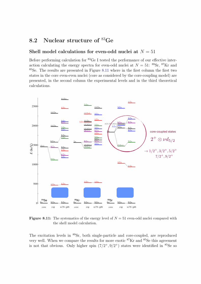
8.2 Nuclear structure of 83Ge

Shell model calculations for even-odd nuclei at N = 51

Before performing calculation for 83Ge I tested the performance of our effective inter-action calculating the energy spectra for even-odd nuclei at N = 51: 89Sr, 87Kr and85Se. The results are presented in Figure 8.11 where in the first column the first twostates in the core even-even nuclei (core as considered by the core-coupling model) arepresented, in the second column the experimental levels and in the third theoreticalcalculations.

Shell Model results at N=51

0

500

1000

1500

2000

2500

EHkeV

L

0+

H2+L

5ê2+

1ê2+

7ê2+

9ê2+

11ê2+

11ê2+

5ê2+

1ê2+

3ê2+9ê2+1ê2+5ê2+

7ê2+5ê2+3ê2+7ê2+9ê2+3ê2+

1ê2+

11ê2+

0+

2+

5ê2+

1ê2+

H7ê2+LH3,5ê2+L9ê2+

H9ê2+LH3,5ê2+LH3,5ê2+L11ê2+H1ê2+L

7ê2+

5ê2+

1ê2+

3ê2+9ê2+5ê2+1ê2+7ê2+9ê2+3ê2+7ê2+1ê2+3ê2+11ê2+

0+

2+

5ê2+

1ê2+

H7ê2+L

5ê2+9ê2+

3ê2+

5ê2+

1ê2+

7ê2+

3ê2+5ê2+9ê2+3ê2+

1ê2+

H1ê2+,3ê2+,5ê2+L3ê2+

1ê2+

core exp n i78-jj4b core exp n i78-jj4b core exp n i78-jj4b

3485Se51 36

87Kr51 3889Sr51

2+ d5/2

8938Sr51

8736Kr51

8534Se51

core-coupled states

88Sr86Kr84Se

! 1/2+, 3/2+, 5/2+, 7/2+, 9/2+

7/2+, 9/2+

Figure 8.11: The systematics of the energy level of N = 51 even-odd nuclei compared withthe shell model calculation.

The excitation levels in 89Sr, both single-particle and core-coupled, are reproducedvery well. When we compare the results for more exotic 87Kr and 85Se this agreementis not that obvious. Only higher spin (7/2+, 9/2+) states were identified in 85Se so

it is difficult to discuss the reliability of our calculation for its excitation states butobviously the 7/2+ is predicted to be too high while 9/2+ is reproduced quite well.The same happens for the 7/2+ state in 87Kr, but the lower spin states and the statewith spin 9/2+ are in relatively good agreement with experiment.

Shell model calculations for 83Ge

The experimental energy spectrum for 83Ge is compared with the shell model calcula-tion in Figure 8.12. On the right side of the figure one can see the calculated groundstate and the first excited 2+ state in 82Ge which has one neutron less than discussed83Ge (and in the weak-coupling model is considered as a core for 83Ge). The wavefunctions of those two states are presented in Table 8.5. One can see that both stateshave contribution from two configurations of protons in the πf 4

5/2 orbit and πp23/2πf

25/2.

Table 8.5: Wave functions of the calculated ground state 0+ and the first 2+ excited statein 82Ge.

Energy exp. [keV] Energy calc. [keV] Jπ Wave function0.0 0.0 0+ 50% πf 4

5/2

33% πp23/2πf

25/2

1347.51(7) 1328 2+ 53% πf 45/2

18% πp23/2πf

25/2

Table 8.6: The experimental energies of excitation levels in 83Ge and proposed calculatedones with the spin assignements and wave functions.

Energy exp. [keV] Energy calc. [keV] Jπ Wave function0.0 0.0 5/2+ 40% πp2

3/2πf25/2 ⊗ νd1

5/2

33% πf 45/2 ⊗ νd1

5/2

247.7(3) 428 1/2+ 40% πp23/2πf

25/2 ⊗ νs1

1/2

20% πf 45/2 ⊗ νs1

1/2

1045.9(4) 1180 3/2+ 35% πf 45/2 ⊗ νd1

5/2

16% πp23/2πf

25/2 ⊗ νd1

5/2

1450 1/2+ 33% πf 45/2 ⊗ νd1

5/2

13% πp23/2πf

25/2 ⊗ νd1

5/2

With our interaction we reproduce well the ground state 5/2+ spin. The wave functionof this state has two components:

• πp23/2πf

25/2 ⊗ νd1

5/2

• πf 45/2 ⊗ νd1

5/2

each with a single neutron in νd5/2 orbital (see Table 8.6). When we compare theproton part of the wave function between 82Ge and 83Ge their compositions differwith the importance of the two components. In case of even-even 82Ge the mostfavourable configuration was of four protons in πf5/2, while when we add one neutronand form 83Ge the configuration of two protons in πp3/2 and two in πf5/2 dominates.This proton configuration is favoured also in the first excited 1/2+ state, also wellreproduced (in terms of spin and energy) by our interaction. This state is formedfrom the excitation of the neutron to the νs1/2 orbital. In the following paragraphs wediscuss the possible spins and parities of the higher excitation levels in 83Ge using theshell model calculations.

0

500

1000

1500

2000

2500

EHke

VL

52+

12+

H12+,32+LH32+,52+LH12+,32+,52+L

H12+,32+,52+L

52+

12+

32+

12+

52+

32+

52+

12+

12+

52+

0+

2+

exp

92+

72+

52+

32+52+72+

92+H12+,32+,52+L

ni78-jj4b Ge "core"

3283Ge51

3282Ge50

Figure 8.12: The resulting level scheme of 83Ge in comparison with theoretical shell modelcalculation made with ni78− jj4b interaction.

Figure 8.13: The schematicview of thepossible electricand magneticmode transi-tions assumingthe 1/2+ or3/2+ spinfor the thirdexcited statein 83Ge. Thenumbers inred representthe partialγ-ray transitionprobabilities.

1045

247.7

05/2+

1/2+

(1/22+)

M1

E2100%

0%

(3/21+) 1045

247.7

05/2+

1/2+

M1+E2

M1+E289%

11%

The level at 1045.9 keV

Two possibilities for the spins for this state are (1/2+) and (3/2+) (as discussed alreadyin Chapter 7). We consider the first calculated 1/2+ state at 1450 keV and the first3/2+ calculated state at 1180 keV as possible candidates for this state. Their wavefunctions are presented in Table 8.6. In both of them the single neutron is in the νd5/2

orbital while protons form similar configurations to the ones seen in 82Ge. There aretwo transitions from the state at 1045.9 keV, one to the ground state and the second tothe first excited state. We proceed with the calculation of the partial γ-ray transitionprobabilities, which can be helpful for the spin assignment.

The two possible scenarios are presented in Figure 8.13 where the considered tran-sitions are of the magnetic M1 and the electric E2 character. The results of thecalculated reduced transition probabilities and the partial γ-ray transition probabili-ties are presented in Table 8.7. From the experimental data, the relative intensitiesof the transition from the state at 1045 keV to the ground state is 90(6)% while theintensity to the first excited state is only 10(2)%. This result is compatible with thecalculated value obtained for the 3/2+ spin state predicted at 1180 keV (89% and 11%).We use this argument for the assignment of the spin 3/2+ for the level at 1045 keV.

The level at 1238 keV

The spin and parity of this level was proposed by Perru [48] to be the 3/2+ or the5/2+ member of the core-particle coupling multiplet since its energy is very close tothe one of the 2+

1 state of 82Ge (1348 keV). The population of this state in β-decay of

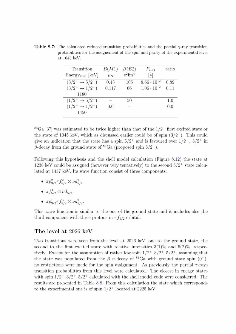
Table 8.7: The calculated reduced transition probabilities and the partial γ-ray transitionprobabilities for the assignement of the spin and parity of the experimental levelat 1045 keV.

Transition B(M1) B(E2) Pi→f ratioEnergylevel [keV] µN e2fm4 [1

s]

(3/2+ → 5/2+) 0.43 105 8.66 · 1012 0.89(3/2+ → 1/2+) 0.117 66 1.06 · 1012 0.11

1180

(1/2+ → 5/2+) – 50 1.0(1/2+ → 1/2+) 0.0 – 0.0

1450

83Ga [37] was estimated to be twice higher than that of the 1/2+ first excited state orthe state of 1045 keV, which as discussed earlier could be of spin (3/2+). This couldgive an indication that the state has a spin 5/2+ and is favoured over 1/2+, 3/2+ inβ-decay from the ground state of 83Ga (proposed spin 5/2−).

Following this hypothesis and the shell model calculation (Figure 8.12) the state at1238 keV could be assigned (however very tentatively) to the second 5/2+ state calcu-lated at 1437 keV. Its wave function consist of three components:

• πp23/2πf

25/2 ⊗ νd1

5/2

• πf 45/2 ⊗ νd1

5/2

• πp13/2πf

35/2 ⊗ νd1

5/2.

This wave function is similar to the one of the ground state and it includes also thethird component with three protons in πf5/2 orbital.

The level at 2026 keV

Two transitions were seen from the level at 2026 keV, one to the ground state, thesecond to the first excited state with relative intensities 3(1)% and 6(2)%, respec-tively. Except for the assumption of rather low spin 1/2+, 3/2+, 5/2+, assuming thatthe state was populated from the β n-decay of 84Ga with ground state spin (0−),no restrictions were made for the spin assignment. As previously the partial γ-raystransition probabilities from this level were calculated. The closest in energy stateswith spin 1/2+, 3/2+, 5/2+ calculated with the shell model code were considered. Theresults are presented in Table 8.8. From this calculation the state which correspondsto the experimental one is of spin 1/2+ located at 2225 keV.

Table 8.8: The calculated reduced transition probabilities and the partial γ-ray transitionprobabilities for the assignement of the spin and parity of the experimental levelsin 83Ge at 2026 keV.

Transition B(M1) B(E2) Pi→f ratioEnergylevel [keV] µN e2fm4 [1

s]

(1/2+3 → 5/2+) – 3.38 8.27 · 1010 0.53

(1/2+3 → 1/2+) 0.0007 – 7.42 · 1010 0.471820

(1/2+4 → 5/2+) – 0.16 1.07 · 1010 0.04

(1/2+4 → 1/2+) 0.012 – 2.33 · 1012 0.962225

(3/2+3 → 5/2+) 0.21 3 31.07 · 1012 0.99

(3/2+3 → 1/2+) 0.0001 0.4 0.009 · 1012 0.11812

(5/2+5 → 5/2+) 0.002 0.006 33.69 · 1010 0.17

(5/2+5 → 1/2+) – 56 180.4 · 1010 0.832000

(5/2+6 → 5/2+) 0.02 2 231.8 · 1010 0.99

(5/2+6 → 1/2+) – 0.32 0.71 · 1010 0.012400

Summary

The final level scheme of 83Ge compared with the theoretical calculation is presentedin Figure 8.14. The possible states were assigned for the 3rd, 4th and 7th excitedstates.

Core-coupled states

As mentioned already earlier, in case of even-odd nuclei we consider single-particle andcore-coupled states. Having assinged the spins and parities of the levels of interest onecan try to make discussion of which of the states in 83Ge is formed by the neutronweak coupling with the even-even core (see Figure 8.15).

We start from the identification of the 9/2+ core-coupled states in N = 51 isotones. Wecompare the wave functions of the first excited 2+ state of even-even core and the core-coupled 9/2+ state in even-odd nuclei (see Figure 8.16). In case of 88,89Sr and 86,87Krthere are two same dominant proton configuration. For 84Se there if one dominant

0

500

1000

1500

2000

2500

EHke

VL

52+

12+

H32+LH52+LH12+,32+,52+L

H12+L

52+

12+

32+

12+

52+

32+

52+

12+

12+

52+

exp

92+

72+

52+

32+52+72+

92+H12+,32+,52+L

ni78-jj4b

3283Ge51

Figure 8.14: The experimental level schemeof 83Ge in comparison with low-spin states obtained in theo-retical calculation made withni78− jj4b interaction.

coupling of the νd5/2 neutron to the first 2+ excitation of the

semi-magic Ν=50 core

2+ d5/2

?

Figure 8.15: Search forthe core-coupledstates inthe experi-mental andtheoreticallevel schemeof 83Ge.

proton configuration and the same in 85Se with one neutron more. We can see thatfor those three nuclei the core-coupling model holds. The same cannot be concludedwhen investigating the wave functions of 83,83Ge and 80,81Zn. The wave function of2+ and 9/2+ states differ and new components appear when one adds neutron to theeven-even core. This new component is dominant (in 83Ge) indicating rahter strongthan weak coupling in this nucleus. One added neutron destroys proton configurationand the connection to the weak core-coupling model is lost. The calculated with theshell model wave functions indicate changes at Z = 32 and Z = 30.

f2 5/2

f4 5/2

p2 3/2

f6 5/2

p2 3/2

f4 5/2

p4 3/2

f5 5/2

p4 3/2

p1 1/2

f6 5/2

p3 3/2

p1 1/2

f2 5/2

p2 3/2

f4 5/2

88Sr 89Sr2+ 9/2+

30%

86Kr 87Kr2+ 9/2+

84Se 85Se2+ 9/2+

82Ge 83Ge2+ 9/2+

60%

80Zn 81Zn2+ 9/2+

f2 5/2

f1 5/2

p1 3/2

f4 5/2

p2 3/2

f6 5/2

p2 3/2

f4 5/2

p4 3/2

f2 5/2

p2 3/2

f5 5/2

p4 3/2

p1 1/2

f6 5/2

p3 3/2

p1 1/2

core configuration same in Sr, Kr, Se

f3 5/2

p1 3/2

→ core-coupling modelcollapse of core-coupling

scheme (ni78-jj4b)

Z=32 Z=30

d5/2

d5/2

d5/2

d5/2

d5/2

proton configuration

%

Figure 8.16: The composition of the wave functions to investigate the core-coupled states.

Chapter 9

Conclusions and outlook

Contents9.1 Conclusions . . . . . . . . . . . . . . . . . . . . . . . . . . . . . . 133

9.2 Outlook . . . . . . . . . . . . . . . . . . . . . . . . . . . . . . . . 135

9.1 Conclusions

The optimization of various steps allowing production of the high-intensity radioactivebeams is necessary and of particular interest for the future radioactive beam facilitieslike SPIRAL2 (GANIL) or EURISOL-DS. The production and separation process in-volves several important steps like powerful primary beam, feasible target material,good extraction and transport, rapidity and selectivity. In order to perform success-fully the experiment of β-decay study we studied and optimized:

• primary beam: The primary beam of electrons used in our experiment to in-duce photo-fission in uranium carbide target intensity 10 µA. The experimentdescribed in this thesis was the commissioning experiment for the ALTO facilityand the first experiment where the electron beam intensity was maximal.

• target: Study of the release properties of different UCx targets was discussed inChapter 4. We studied different samples of uranium carbide targets in order tofind the most optimal one that will be used, at first in our experiment, and laterin SPIRAL2. The samples were first irradiated with deuteron beam of energy26 MeV and intensity 20 nA and in the next step heated in the oven up to1200 C. The activities from the pellets were measured after the heating with twogermanium detectors. I performed simulations of the expected γ-ray spectrumto determine the feasibility of the experiment and the estimation of the expectedcounting rate.

• selectivity: For the ionization of gallium atoms we used newly developed laserionization source. The gallium atoms were ionized in two steps: the first laserbeam was used to excite the electron which was then ejected with the secondlaser beam. The efficiency of this source was estimated to be 10 times higher

than the surface ionization source (from the test of the stable 69Ga beam). Thislaser ion souce was successfully used during our experiment. The comparisonspectrum between the data acquired with and without the laser was presentedin Figure 5.15.

Except for the optimization of the production, release and ionization of the fissionproducts the detection system in the low-count rate β-decay study plays a very im-portant role. Due to exoticity of the elements studied the statistics is low and it isdesirable to have detection system with high enough efficiency and shielded from thebackground. I tested the performance of newly designed BGO shield (prototype forthe ORGAM2 project at ALTO), and the Veto plastic detector. This study was per-formed in order to test the background subtraction in the configuration of germaniumdetector surrounded with BGO shield and the Veto plastic. This configuration withfive germanium detectors surrounding the collection point is done in the new detec-tion system BEDO (BEta Decay studies at Orsay). This detection system is currentlycommissioned at ALTO.

A priori to the experimental study of the β-decay of neutron rich gallium I built ashell model interaction in collaboration with K. Sieja and F. Nowacki from IPHC(Strasbourg). The new ni78− jj4b interaction has the following properties:

• 78Ni core,

• valence space for protons is 2p3/2, 1f5/2, 2p1/2 and 1g9/2,

• valence space for neutrons: 1g7/2, 2d5/2, 2d3/2, 3s1/2, 1h11/2.

I built the effective interaction which can reproduce well already known experimentaldata and which has predictive power for our nuclei of interest. I successfully used theni78 − jj4b interaction to perform theoretical calculation for excitation energies andreduced transition probabilities for 83−84Ge.

We performed experimental studies to probe the nuclear structure of the neutron-rich nuclei in the vicinity of 78Ni via β-decay spectroscopy of 84Ga. Using time spectraI discriminated half-lives of the mother nuclei. With γ−γ coincidences new transitionswere found which allowed us to improve levels schemes of:

• N = 51 even-odd 83Ge: The constraints were put for the spin assignment of allthe levels identified. Using shell model predictions I made tentative assignmentof spins and parities to three of the states.

• N = 52 even-even 84Ge: The third excitation state was assigned as 2+2 possibly

belonging to the γ-band, as predicted by the shell model calculation. From theDavydov’s model, 84Ge is seen to have rigid asymmetry of γ ≈ 25. Similaritiesin the dynamics were found when comparing with 80Ge.

• N = 51 odd-odd 84As: Many new excited states and γ-transitions were found inthis nucleus. This odd-odd nucleus is difficult to interpret with our shell modelinteraction and more theoretical work should be done in order to obtain reliableconclusions on the structure of 84As.

9.2 Outlook

The experiment of β-decay described in this thesis was one of the few commissioningtests performed at the ALTO facility. After this successful run the safety authorityhas given in May 2012 the official authorization for the exploitation of ALTO. A broadphysics program is planned for the up-coming years:

• work on the studies of differently manufactured UCx targets continues, new pro-totypes are manufactured and tested,

• experiments are planned with thorium carbide target in order to reach elementswith lower masses (close to N = 50) in fission reaction,

• the newly built detection system BEDO dedicated to study β-decay of radioac-tive species has been recently built and commissioned at ALTO. It has higherefficiency (absolute efficiency estimated to 5−6% as compared with 2% efficiencyof the system with two germanium detectors used in previous experiments). Thefuture experiment planned is β-decay study of 81Cu to populate excited statesin 81Zn,

• new neutron detector Tetra has been built at IPN Orsay in collaboration withDubna (Russia). Next experiments are planned with full intensity 10µA electronbeam and laser ion source to study the neutron emission probability of neutronrich gallium (85−86Ga) using this neutron detector and germanium detector.

Bibliography

[1] C. Engelmann, Z. Phys. A 352, 351 (1995). (Cited on page 1.)

[2] K. Sieja, F. Nowacki, K. Langanke and G. Martinez-Pinedoz, Physical ReviewC 79, 064310 (2009). (Cited on pages 1 and 28.)

[3] J. Duflo and A.P. Zuker, Phys. Rev. C 59, R2347 (1999). (Cited on page 1.)

[4] T. Otsuka, T. Matsuo and D. Abe, Phys. Rev. Lett. 97, 162501 (2006). (Citedon page 1.)

[5] T. Otsuka, T. Suzuki, M. Honma, Y. Utsuno, N. Tsun-oda, K. Tsukiyama andM. Hjorth-Jensen, Phys. Rev. Lett. 104, 012501 (2010). (Cited on page 1.)

[6] K.T. Flanagan, P. Vingerhoets, M. Avgoulea, J. Billowes, M.L. Bissell, K. Blaum,B. Cheal, M. De Rydt, V.N. Fedosseev, D.H. Forest, C. Geppert, U. Köster,M. Kowalska, J. Krämer, K.L. Kratz, A. Krieger, E. Mané, B.A. Marsh, T. Ma-terna, L. Mathieu, P.L. Molkanov, R. Neugart, G. Neyens, W. Nörtershäuser,M.D. Seliverstov, O. Serot, M. Schug, M.A. Sjoedin, J.R. Stone, N.J. Stone,H.H. Stroke, G. Tungate, D.T. Yordanov and Y.M. Volkov, Phys. Rev. Lett.103, 142501 (2009). (Cited on page 1.)

[7] T. Otsuka, T. Suzuki, R. Fujimoto, H. Grawe and Y. Akaishi, Phys. Rev. Lett.95, 232502 (2005). (Cited on page 1.)

[8] B. Fogelberg, Phys. Rev. Lett. 73, 2413 (1994). (Cited on page 2.)

[9] K.L. Jones, A.S. Adekola, D.W. Bardayan, J.C. Blackmon, K.Y. Chae, K.A.Chipps, J.A. Cizewski, L. Erikson, C. Harlin, R. Hatarik, R. Kapler, R.L. Kozub,J.F. Liang, R. Livesay, Z. Ma, B.H. Moazen, C.D. Nesaraja, F.M. Nunes, S.D.Pain, N.P. Patterson, D. Shapira, J.F.S. Jr, M.S. Smith, T.P. Swan and J.S.Thomas, Nature 465, 454 (2010). (Cited on page 2.)

[10] B. Bastin, S. Grévy, D. Sohler, O. Sorlin, Z. Dombrádi, N.L. Achouri, J.C.Angélique, F. Azaiez, D. Baiborodin, R. Borcea, C. Bourgeois, A. Buta,A. Bürger, R. Chapman, J.C. Dalouzy, Z. Dlouhy, A. Drouard, Z. Elekes, S. Fran-choo, S. Iacob, B. Laurent, M. Lazar, X. Liang, E. Liénard, J. Mrazek, L. Nalpas,F. Negoita, N.A. Orr, Y. Penionzhkevich, Z. Podolyák, F. Pougheon, P. Roussel-Chomaz, M.G. Saint-Laurent, M. Stanoiu, I. Stefan, F. Nowacki and A. Poves,Phys. Rev. Lett. 99, 022503 (2007). (Cited on page 2.)

[11] M. Stanoiu, D. Sohler, O. Sorlin, F. Azaiez, Z. Dombrádi, B.A. Brown, M. Bel-leguic, C. Borcea, C. Bourgeois, Z. Dlouhy, Z. Elekes, Z. Fülöp, S. Grévy,D. Guillemaud-Mueller, F. Ibrahim, A. Kerek, A. Krasznahorkay, M. Lewitow-icz, S.M. Lukyanov, S. Mandal, J. Mrázek, F. Negoita, Y.E. Penionzhkevich,Z. Podolyák, P. Roussel-Chomaz, M.G. Saint-Laurent, H. Savajols, G. Sletten,J. Timár, C. Timis and A. Yamamoto, Phys. Rev. C 78, 034315 (2008). (Citedon page 2.)

[12] M.G. Porquet and O. Sorlin, Phys. Rev. C 85, 014307 (2012). (Cited on pages 2and 3.)

[13] O. Sorlin and M. Porquet, Progress in Particle and Nuclear Physics 61, 602–673(2008). (Cited on pages 2 and 7.)

[14] J. Hakala, S. Rahaman, V.V. Elomaa, T. Eronen, U. Hager, A. Jokinen,A. Kankainen, I.D. Moore, H. Penttilä, S. Rinta-Antila, J. Rissanen, A. Saas-tamoinen, T. Sonoda, C. Weber and J. Äystö, Phys. Rev. Lett. 101, 052502(2008). (Cited on page 3.)

[15] M. Bender, G.F. Bertsch and P.H. Heenen, Phys. Rev. C 78, 054312 (2008).(Cited on page 3.)

[16] H. Fann, J. Schiffer and U. Stohbush, Phys. Lett. B 44, 19 (1973). (Cited onpages 3 and 5.)

[17] P. Li, W. Daehnick, S.K. Saha, J. Brown and R. Kouzes, Nulc. Phys. A 469,393–406 (1987). (Cited on pages 3 and 5.)

[18] G. Winter, R. Schwengner, J. Reif, H. Prade, L. Funke, R. Wirowski, N. Nicolay,A. Dewald, P. v Brentano, H. Grawe and R. Schubart, Phys. Rev. C 48, 1010–1019 (1993). (Cited on pages 3 and 5.)

[19] A. Prevost, M. Porquet, A. Astier, I. Deloncle, F. Azaiez, A. Buta, D. Curien,O. Dorvaux, G. Duchene, B. Gall, F. Khalfallah, I. Piqueras, M. Rousseau,M. Meyer, N. Redon, O. Stezowski, T. Venkova, R. Lucas and A. Bogachev,Eur. Phys. J. A 22, 391–395 (2004). (Cited on pages 3 and 5.)

[20] T. Rząca-Urban, W. Urban, J.L. Durell, A.G. Smith and I. Ahmad, Phys. Rev.C 76, 027302 (2007). (Cited on pages 3, 4, 5 and 6.)

[21] Y.H. Zhang, Z. Podolyàk, G.d. Angelis, A. Gadea, C. Ur, S. Lunardi,N. Marginean, C. Rusu, R. Schwengner, T. Kröll, D.R. Napoli, R. Menegazzo,D. Bazzacco, E. Farnea, S. Lenzi, T. Martinez, M. Axiotis, D. Tonev, W. Gel-letly, S. Langdown, P.H. Regan, J.J. Valiente Dobon, W. v Oertzen, B. Rubio,

B. Quintana, N. Medina, R. Broda, D. Bucurescu, M. Ionescu-Bujor and A. Ior-dachescu, Phys. Rev. C 70, 024301 (2004). (Cited on page 4.)

[22] F.N. K. Sieja, arXiv:1201.0373 (2012). (Cited on pages 4 and 5.)

[23] S. Raman, C.W.Nestor and P.Tikkanen, At. Data Nucl. Data Tables 78, 1 (2001).(Cited on pages 7 and 13.)

[24] E. Padilla-Rodal, A. Galindo-Uribarri, C. Baktash, J.C. Batchelder, J.R. Beene,R. Bijker, B.A. Brown, O. Castaños, B. Fuentes, J.G. d Campo, P.A. Hausladen,Y. Larochelle, A.F. Lisetskiy, P.E. Mueller, D.C. Radford, D.W. Stracener, J.P.Urrego, R.L. Varner and C.H. Yu, Phys. Rev. Lett. 94, 122501 (2005). (Citedon pages 5, 6 and 7.)

[25] A. Gade, T. Baugher, D. Bazin, B.A. Brown, C.M. Campbell, T. Glas-macher, G.F. Grinyer, M. Honma, S. McDaniel, R. Meharchand, T. Otsuka,A. Ratkiewicz, J.A. Tostevin, K.A. Walsh and D. Weisshaar, Phys. Rev. C 81,064326 (2010). (Cited on page 7.)

[26] R. Lecomte, M. Irshad, S. Landsberger, G. Kajrys, P. Paradis and S. Monaro,Phys. Rev. C 22, 2420–2423 (1980). (Cited on page 5.)

[27] W.T. Chou, D.S. Brenner, R.F. Casten and R.L. Gill, Phys. Rev. C 47, 157–162(1993). (Cited on pages 5 and 6.)

[28] A. Makishima, M. Asai, T. Ishii, I. Hossain, M. Ogawa, S. Ichikawa and M. Ishii,Phys. Rev. C 59, R2331–R2333 (1999). (Cited on page 5.)

[29] Y. Toh, T. Czosnyka, M. Oshima, T. Hayakawa, H. Kusakari, M. Sugawara,Y. Hatsukawa, J. Katakura, N. Shinohara and M. Matsuda, The Eur. Phys.Journal A - Hadrons and Nuclei 9, 353–356 (2000). (Cited on pages 5 and 6.)

[30] M. Sugawara, Y. Toh, T. Czosnyka, M. Oshima, T. Hayakawa, H. Kusakari,Y. Hatsukawa, J. Katakura, N. Shinohara, M. Matsuda, T. Morikawa, A. Sekiand F. Sakata, The Eur. Phys. Journal A - Hadrons and Nuclei 16, 409–414(2003). (Cited on page 5.)

[31] H. Iwasaki, S. Michimasa, M. Niikura, M. Tamaki, N. Aoi, H. Sakurai, S. Shi-moura, S. Takeuchi, S. Ota, M. Honma, T.K. Onishi, E. Takeshita, H.J. Ong,H. Baba, Z. Elekes, T. Fukuchi, Y. Ichikawa, M. Ishihara, N. Iwasa, S. Kanno,R. Kanungo, S. Kawai, T. Kubo, K. Kurita, T. Motobayashi, A. Saito, Y. Satou,H. Suzuki, M.K. Suzuki, Y. Togano and Y. Yanagisawa, Phys. Rev. C 78, 021304(2008). (Cited on pages 5, 6 and 120.)

[32] B. Kotliński, T. Czosnyka, D. Cline, J. Srebrny, C. Wu, A.B.L. Hasselgren,L. Westerberg, C. Baktash and S. Steadman, Nucl. Phys. A 519, 646–658 (1990).(Cited on page 6.)

[33] R. Lecomte, G. Kajrys, S. Landsberger, P. Paradis and S. Monaro, Phys. Rev.C 25, 2812–2814 (1982). (Cited on page 6.)

[34] P. Hoff and B. Fogelberg, Nucl. Phys. A 368, 210 (1981). (Cited on page 6.)

[35] B. Tastet, Structure des noyaux de gallium, de germanium et d’arsenic riches enneutrons autour de n=50 et dèveloppement d’une source d’ionisation laser à alto,Université Paris-Sud 11, (2011). (Cited on pages 6, 9, 58, 60, 65, 98 and 102.)

[36] D. Verney, B. Tastet, K. Kolos, F.L. Blanc, F. Ibrahim, M.C. Mhamed, E. Cot-tereau, P.V.Cuong, F. Didierjean, G. Duchene, S. Essabaa, M. Ferraton, S. Fran-choo, L. Khiem, C. Lau, J.F.L. Du, I. Matea, B. Mouginot, M. Niikura, B. Rouss-siére, I. Stefan, D. Testov and J.C. Thomas. Study of the β-decay of 80ga: addi-tional elements on the proton structure on n=48,49 isotones toards z=28. to bepublished. (Cited on page 6.)

[37] J.A. Winger, K.P. Rykaczewski, C.J. Gross, R. Grzywacz, J.C. Batchelder,C. Goodin, J.H. Hamilton, S.V. Ilyushkin, A. Korgul, W. Królas, S.N. Lid-dick, C. Mazzocchi, S. Padgett, A. Piechaczek, M.M. Rajabali, D. Shapira, E.F.Zganjar and J. Dobaczewski, Phys. Rev. C 81, 044303 (2010). (Cited on pages 6,7, 9, 70, 90, 94, 95, 96, 98, 104, 105, 106, 109 and 129.)

[38] U. Koster. Workshop on neutron rich nuclei, 16-20 Mars 2008. (Cited on pages 7,90 and 94.)

[39] M. Lebois, D. Verney, F. Ibrahim, S. Essabaa, F. Azaiez, M.C. Mhamed, E. Cot-tereau, P.V. Cuong, M. Ferraton, K. Flanagan, S. Franchoo, D. Guillemaud-Mueller, F. Hammache, C. Lau, F. Le Blanc, J.F. Le Du, J. Libert, B. Mouginot,C. Petrache, B. Roussière, L. Sagui, N. d Séréville, I. Stefan and B. Tastet, Phys.Rev. C 80, 044308 (2009). (Cited on pages 7, 67, 90, 94, 96, 106, 108 and 116.)

[40] S. Padgett, M. Madurga, R. Grzywacz, I.G. Darby, S.N. Liddick, S.V.Paulauskas, L. Cartegni, C.R. Bingham, C.J. Gross, K. Rykaczewski, D. Shapira,D.W. Stracener, A.J. Mendez, J.A. Winger, S.V. Ilyushkin, A. Korgul,W. Królas, E. Zganjar, C. Mazzocchi, S. Liu, J.H. Hamilton, J.C. Batchelderand M.M. Rajabali, Phys. Rev. C 82, 064314 (2010). (Cited on page 7.)

[41] T.A. Hughes, Phys. Rev. 181, 1586–1596 (1969). (Cited on page 8.)

[42] E.A. Henry, W.L. Talbert and J.R. McConnell, Phys. Rev. C 7, 222–238 (1973).(Cited on page 8.)

[43] S.M. Abecasis, J. Davidson and M. Davidson, Phys. Rev. C 22, 2237–2242(1980). (Cited on page 8.)

[44] J.S. Thomas, G. Arbanas, D.W. Bardayan, J.C. Blackmon, J.A. Cizewski, D.J.Dean, R.P. Fitzgerald, U. Greife, C.J. Gross, M.S. Johnson, K.L. Jones, R.L.Kozub, J.F. Liang, R.J. Livesay, Z. Ma, B.H. Moazen, C.D. Nesaraja, D. Shapira,M.S. Smith and D.W. Visser, Phys. Rev. C 76, 044302 (2007). (Cited on pages 8,9, 95 and 98.)

[45] N.A. Detorie, P.L. Jolivette, C.P. Browne and A.A. Rollefson, Phys. Rev. C 18,991–1002 (1978). (Cited on page 8.)

[46] A. Saganek, V. Meyer, S. Mirowski, M. Oteski, M. Sieminski, E. Wesolowski andZ. Wilhelmi, J. Phys. 10, 549 (1984). (Cited on page 8.)

[47] J.S. Thomas, D.W. Bardayan, J.C. Blackmon, J.A. Cizewski, U. Greife, C.J.Gross, M.S. Johnson, K.L. Jones, R.L. Kozub, J.F. Liang, R.J. Livesay, Z. Ma,B.H. Moazen, C.D. Nesaraja, D. Shapira and M.S. Smith, Phys. Rev. C 71,021302 (2005). (Cited on pages 9, 95 and 98.)

[48] O. Perru, Eur. Phys. J. A 28, 307 – 312 (2006). (Cited on pages 9, 53, 95, 96,98 and 128.)

[49] M. Lebois, Structure des noyaux de germanium et de gallium riches en neutronsau-delà de N = 50 à alto, Université Paris-Sud 11, (2008). (Cited on pages 9,67, 83, 95, 98 and 102.)

[50] J.V. Kratz, Nucl. Phys. A 250, 13 (1975). (Cited on pages 9 and 102.)

[51] J. Omtvedt, B. Fogelberg and P. Hoff, Z. Phys. A 339, 349 (1991). (Cited onpages 9, 98 and 102.)

[52] J.A. Winger. Failure of the 78Ni core for Z > 28, N > 50, 2007. (Cited onpages 9, 98 and 102.)

[53] R. Casten, Nuclear Structures from a Simple Perspective, Oxford UniversityPress, (1990). (Cited on pages 11, 13, 17, 18 and 20.)

[54] G. Gamow, Proc. Roy. Soc. [A] 136, 386–387 (1929). (Cited on page 12.)

[55] G. Gamow, Proc. Roy. Soc. [A] 126, 632–644 (1930). (Cited on page 12.)

[56] N. Bohr, Nature 137, 344–348 (1936). (Cited on page 12.)

[57] N. Bohr and J.A. Wheeler, Phys.Rev. 56, 426–450 (1939). (Cited on page 12.)

[58] C. Weizsacker, Z.Phys. 96, 431–458 (1935). (Cited on page 12.)

[59] F. Nowacki. Structure en couche des noyaux: de la stabilité à la limited’existance, jolie-curies school, 2002. (Cited on page 15.)

[60] M. Goeppert-Mayer, Phys. Rev. 75, 1969 (1949). (Cited on page 15.)

[61] O. Haxel, J. Hans, D. Jensen and H.E. Suess, Phys. Rev. 75, 1766 (1949). (Citedon page 15.)

[62] A. Davydov and G. Filippov, Nucl .Phys. 8, 237–249 (1958). (Cited on pages 17,18, 19, 118, 119 and 123.)

[63] B.A. Brown, Lecture Notes in Nuclear Structure Physics, National Superconduct-ing Cyclotron Laboratory and Department of Physics and Astronomy, MichiganState University, (2005). (Cited on page 21.)

[64] B.J. Brussaard and P.W.M. Glaudemans, Shell Model applications in nuclearspectroscopy, North Holland Publishing Company, (1977). (Cited on page 22.)

[65] N. Smirnova. Shell structure evolution and effective in-medium nn interaction,ecole jolie curie, 2009. (Cited on pages 23 and 24.)

[66] S. Bogner, R. Furnstahl and A. Schwenk, Progress in Particle and NuclearPhysics 65, 94–147 (2010). (Cited on page 25.)

[67] S. Bogner, T. Kuo and L. Coraggio, Nuclear Phys. A 684, 432 (2001). (Citedon page 25.)

[68] S. Bogner, Phys. Rev. C 2002, 051301 (65). (Cited on page 25.)

[69] A. Poves and A. Zuker, Phys. Rep. 70, 235 (1981). (Cited on page 25.)

[70] G. Martinez-Pinedo, A. Zuker, A. Poves and E. Caurier, Phys. Rev. C 55, 187(1997). (Cited on page 25.)

[71] F. Nowacki, Description microscopique des processus faibles dans les noyauxspheriques, IReS Strasbourg school, (1996). (Cited on page 25.)

[72] M. Homna, T. Otsuka, B.A. Brown and T. Mizusaki, Phys. Rev. C 65,061301(R) (2002). (Cited on page 25.)

[73] T. Otsuka, M. Homna and T. e al., Prog. Part. Nucl. Phys. 47, 319 (2001).(Cited on page 25.)

[74] M. Dufour and A. Zuker, Phys. Rev. C 54, 1641 (1996). (Cited on pages 25and 26.)

[75] E. Caurier and F. Nowacki, Acta Physica Polonica B 30, 705 (1999). (Cited onpage 27.)

[76] A. Poves and F. Nowacki, Lecture Notes in Physics 581, 70 (2001). (Cited onpage 27.)

[77] J.A. Winger, J.C. Hill, F.K. Wohn, R.L. Gill, X. Ji and B.H. Wildenthal, Phys.Rev. C 38, 285–294 (1988). (Cited on page 28.)

[78] D. Verney, F. Ibrahim, C. Bourgeois, S. Essabaa, S. Galès, L. Gaudefroy,D. Guillemaud-Mueller, F. Hammache, C. Lau, F.L. Blanc, A.C. Mueller,O. Perru, F. Pougheon, B. Roussière, J. Sauvage and O. Sorlin, Phys. Rev.C 76, 054312 (2007). (Cited on pages 28 and 53.)

[79] F. Clapier, A.C. Mueller, J. Obert, O. Bajeat, M. Ducourtieux, A. Ferro, A. Hor-bowa, L. Kotfila, C. Lau, H. Lefort, S. Kandri-Rody, N. Pauwels, J.C. Potier,J. Proust, J.C. Putaux, C.F. Liang, P. Paris, A.C.C. Villari, R. Lichtenthäler,L. Maunoury and J. Lettry, Phys. Rev. ST Accel. Beams 1, 013501 (1998). (Citedon pages 36 and 53.)

[80] H. Ravn and B. Allardyce, Treatise on Heavy-Ion Science; Plenum Press, NewYork 8 (1989). (Cited on page 36.)

[81] K. Peräjärvi, U.C. Bergmann, V.N. Fedoseyev, A. Joinet, U. Köster, C. Lau,J. Lettry, H. Ravn and M. Santana-Leitner, Nucl. Inst.and Meth. in PhysicsResearch Section B: Beam Interactions with Materials and Atoms 204, 272 –277 (2003). (Cited on page 36.)

[82] B. Roussière, F. Ibrahim, J. Sauvage, O. Bajeat, N. Barré, F. Clapier, E. Cot-tereau, C. Donzaud, M. Ducourtieux, S. Essabaa, D. Guillemaud-Mueller,C. Lau, H. Lefort, C.F. Liang, F.L. Blanc, A.C. Mueller, J. Obert, N. Pauwels,J.C. Potier, F. Pougheon, J. Proust, O. Sorlin, D. Verney and A. Wojtasiewicz,Nucl. Inst. and Meth. in Physics Research Section B: Beam Interactions withMaterials and Atoms 194, 151 – 163 (2002). (Cited on page 36.)

[83] B. Roussière, O. Bajeat, N. Barré, C. Bourgeois, F. Clapier, E. Cottereau,C. Donzaud, M. Ducourtieux, S. Essabaa, D. Guillemaud-Mueller, F. Ibrahim,C. Lau, F.L. Blanc, H. Lefort, C. Liang, A. Mueller, J. Obert, N. Pauwels,J. Potier, F. Pougheon, J. Proust, J. Sauvage, O. Sorlin, D. Verney and A. Wo-jtasiewicz, Nucl. Instr. and Meth. in Physics Research Section B: Beam Interac-tions with Materials and Atoms 246, 288 – 296 (2006). (Cited on page 36.)

[84] CEA/CNRS. Technical report of the radioactive beam section, 2007. (Cited onpage 36.)

[85] H. Bateman, Proc. Cambridge Phil. Soc. 16, 423 (1910). (Cited on page 40.)

[86] Nuclear data sheets. http://www.nndc.bnl.gov/nds/. (Cited on pages 42, 43,105 and 106.)

[87] T. England and B. Rider. Fission product yields per 100 fissions for 238u high-energy neutron fission decay. LA-UR-94-3106, ENDF-349. (Cited on page 42.)

[88] B. Hy, N. Barre-Boscher, A. Ozgumus, B. Roussiere, S. Tusseau-Nenez, C. Lau,M.C. Mhamed, M. Raynaud, A. Said, K. Kolos, E. Cottereau, S. Essabaa,O. Tougait and M. Pasturel, Nuclear Instruments and Methods in Physics Re-search Section B: Beam Interactions with Materials and Atoms 288, 34 – 41(2012). (Cited on page 49.)

[89] C. Lau, Etude de la production de faisceaux riches en neutrons par fission induitepar neutrons rapides, ph. d. thesis, Université Denis Diderot - Paris VII, (2000).(Cited on pages 53 and 68.)

[90] C. Lau, B. Roussière, D. Verney, O. Bajeat, F. Ibrahim, F. Clapier, E. Cottereau,C. Donzaud, M. Ducourtieux, S. Essabaa, D. Guillemaud-Mueller, F. Hosni,H. Lefort, F.L. Blanc, A. Mueller, J. Obert, N. Pauwels, J. Potier, F. Pougheon,J. Proust, J. Sauvage and A. Wojtasiewicz, Nucl. Instr. and Meth. in PhysicsResearch B 204, 246–250 (2003). (Cited on page 53.)

[91] F. Ibrahim, Eur. Phys. J. A 15, 357 (2002). (Cited on page 53.)

[92] F. Ibrahim, D. Verney, M. Lebois, B. Roussiére, S. Essabaa, S. Franchoo,S. Gales, D.G. Mueller, C. Lau, F.L. Blanc, J.L. Du, M. Mhamed, A. Muellerand J. Sauvage, Nuclear Physics A 787, 110 – 117 (2007). (Cited on page 53.)

[93] T. v Egidy, F.J. Hartmann, D. Habs, K. Lobner and H. Niefneker, World Scien-tific, Singapore, 54 (1997). (Cited on page 53.)

[94] P. Lestone and A. Gavron, Phys. Rev. C 49, 372 (1994). (Cited on pages 53and 54.)

[95] N. Pauwels, University Paris Sud 11, (1998). (Cited on page 54.)

[96] M. Mirea, R. V. A. al. Il Nuovo Cimento A 111, 267 (1998). (Cited on page 54.)

[97] C.M. Zoller, Fachbereich Physik der Technischen Hochschule Darmstadt, (1995).(Cited on page 55.)

[98] W. Diamond, Nucl. Inst. and Meth. A 432, 471 (1999). (Cited on page 54.)

[99] Y. Oganessian, Nuclear Physics A 701, 87 – 95 (2002). (Cited on pages 54and 56.)

[100] U. Köster, Ausbeuten und spektroskopie radioaktiver isotope bei lohengrin undisolde, Physik-Department der Technischen Universität München, (1999). (Citedon pages 57, 64 and 65.)

[101] R. Kirchner, Nucl. Instr. and Meth. in Physics Research Section A: Accelerators,Spectrometers, Detectors and Associated Equipment 292, 203 – 208 (1990).(Cited on page 57.)

[102] S. Sundell, Nucl. Instr. and Meth. B 70, 160 (1992). (Cited on pages 58 and 59.)

[103] R. Kirchner and E. Roecki, Nucl. Inst. Meth. A 133, 187 – 204 (1976). (Citedon page 58.)

[104] W. Jesse and J. Sadauskis, Phys. Rev. 100, 1755 (1955). (Cited on page 59.)

[105] G. Hurst, Rev. Mod. Phys. 51 (1979). (Cited on page 59.)

[106] H. Friedrich, Theoretical Atomic Physics, Springer, Berlin, Heidelberg, (1998).(Cited on page 61.)

[107] L.J. Radziemski, Reference data on atoms, molecules end ions, Springer, (1985).(Cited on page 61.)

[108] R.V. Ambartsumyan, JETP Lett. 21, 276 (1975). (Cited on page 61.)

[109] E.F. Worden, R.W. Solarz, J.A. Paisner and J.G. Conway, J. Opt. Soc. Am. 68,52 –61 (1978). (Cited on page 61.)

[110] M.C. Mhamed, Production des noyaux exotiques par photofission. le projectalto : Premieres resultats, Universite d’Evry Val d’Essone, (2006). (Cited onpage 62.)

[111] P. Paris, C. Liang, D. Lecouturier, M. Arianer, J. Obert, A. Caruette, A. Ferro,J. Fournet, J. Putaux and J. Sarrouy, Nucl. Inst. and Meth. in Physics Research186, 91 – 98 (1981). (Cited on page 68.)

[112] J.C. Putaux, Nucl. Instr. and Meth., 321 (1981). (Cited on page 68.)

[113] K.-L.Kratz, H.Gabelmann, P.Mollear, B.Pfeiffer, H.L.Ravn, A.Wohr andt ISOLDE Collaboration, Z.Phys. A 340, 419 (1991). (Cited on pages 71, 86,90, 104 and 105.)

[114] D. Abriola, M. Bostan, S. Erturk, M. Fadil, M. Galan, S. Juutinen, T. Kibédiand F. Kondev, Nuclear Data Sheets 110, 2815–2944 (2009). (Cited on page 76.)

[115] G.F. Knoll, Radiation detection and measurement, John Wiley & Sons, (1979).(Cited on pages 78 and 81.)

[116] National nuclear data center, logft calculator. http://www.nndc.bnl.gov/logft/. (Cited on pages 81, 93, 94 and 107.)

[117] J. Bris, R. Sellem, J. Artiges, J.F. Clavelin, S. Du, X. Grave, O. Hubert,J. Sauvage and B. Roussire. Notice de l’acquisition comet-narval. institut dephysique nucléaire, 2005. (Cited on page 83.)

[118] I.N. Borzov, Phys. Rev. C 71, 065801 (2005). (Cited on page 104.)

[119] E. Caurier, A. Poves and A.P. Zuker, Phys. Rev. Lett. 74, 1517–1520 (1995).(Cited on page 117.)

[120] P. v Neumann-Cosel, Phys. Lett. B443, 1 (1996). (Cited on page 117.)

[121] E. Caurier, G. Martinez-Pinedo, F. Nowacki, A. Poves and A. Zuker, Reviewsof Modern Physics 77, 427–488 (2005). (Cited on page 117.)

[122] V. Werner, N. Pietralla, P. v Brentano, R.F. Casten and R.V. Jolos, Phys. Rev.C 61, 021301 (2000). (Cited on page 121.)

[123] V. Werner, P. v Brentano and R. Jolos, Physics Letters B 521, 146 – 152 (2001).(Cited on page 121.)

[124] V. Werner, C. Scholl and P.v. Brentano, Phys. Rev. C 71, 054314 (2005). (Citedon page 121.)

[125] J.P. Delaroche, M. Girod, J. Libert, H. Goutte, S. Hilaire, S. Peru, N. Pillet andG.F. Bertsch, Phys. Rev. C 81, 014303 (2010). (Cited on page 123.)

[126] CEA. Beyond mean field calculations www.phynu.cea.fr. (Cited on pages 123and 124.)