probably the best simple pid tuning rules in the...
TRANSCRIPT
Probably the best simple PID tuning rules in the world
Sigurd Skogestad�
Department of Chemical Engineering
Norwegian University of Science and Technology
N–7491 Trondheim Norway
Submitted to Journal of Process Control July 3, 2001This version: July 17, 2001
Abstract
The aim of this paper is to present analytic tuning rules which are as simple as possible and stillresult in a good closed-loop behavior. The starting point has been the IMC PID tuning rules of Rivera,Morari and Skogestad (1986) which have achieved widespread industrial acceptance. The integral termhas been modified to improve disturbance rejection for integrating processes. Furthermore, rather thanderiving separate rules for each transfer function model, we start by approximating the process by afirst-order plus delay processes (e.g. using the “half method”), and then use a single tuning rule. This ismuch simpler and appears to give controller tunings with comparable performance.
1 Introduction
Hundreds, if not thousands, of papers have been written on tuning of PID controllers, and one must questionthe need for another one. The first justification is that PID controller is by far the most widely used controlalgorithm in the process industry, and that improvements in tuning of PID controllers will have a significantpractical impact. The second justification is that the simple rules and insights presented in this paper maycontribute to a significantly improved understanding into how the controller should be tuned.
The PID controller has three principal control effects. The proportional (P) action gives a change inthe input (manipulated variable) directly proportional to the control errorr. The integral (I) action gives achange in the input proportional to the integrated error, and its main purpose is to eliminate offset. Theless commonly used derivative (D) action is used in some cases to speed up the response or to stabilizethe system, and it gives a change in the input proportional to the derivative of the controlled variable. Theoverall controller output is the sum of the contributions from these three terms. The corresponding threeadjustable PID parameters are most commonly selected to be
� Controller gainKc (increased value gives more proportional action and faster control)
� Integral time�I [s] (decreased value gives more integral action and faster control)
� Derivative time�D [s] (increased value gives more derivative action and faster control)
�E-mail: [email protected]; Phone: +47-7359-4154
1
Although the PID controller has only three parameters, it is not easy, without a systematic procesure,to find good values (tunings) for them. In fact, a visit to a process plant will usually show that a largenumber of the PID controllers are poorly tuned. The objective of this paper is to simple model-based tuningrules that give insight into how the tuning depends on the process parameters based on very simple processinformation. These rules may then be used to assist in retuning the controller if, for example, the productionrate is changed. Another related objective is that the rules should be so simple that they can be memorized.
There has been previous work along these lines; most noteworthy the early paper by Ziegler and Nichols(1942), the IMC PID-tuning paper by Rivera, Morari and Skogestad (1986), and the book by Smith andCorripio (1985). The Ziegler-Nichols tunings result in a very good disturbance response for integratingprocesses, but are otherwise known to result in rather aggressive tunings (e.g., Tyreus and Luyben (1992)),and also give poor performance for processes with a dominant delay. On the other hand, the IMC-tunings ofRiveraet al. (1986) are known to result in poor disturbance response for integrating processes (e.g., Chienand Fruehauf (1990), Hornet al. (1996)), but generally give very good responses for setpoint changes.
ee q- - - -?
?
-6
ys y++
gd
gc-
+ u
d
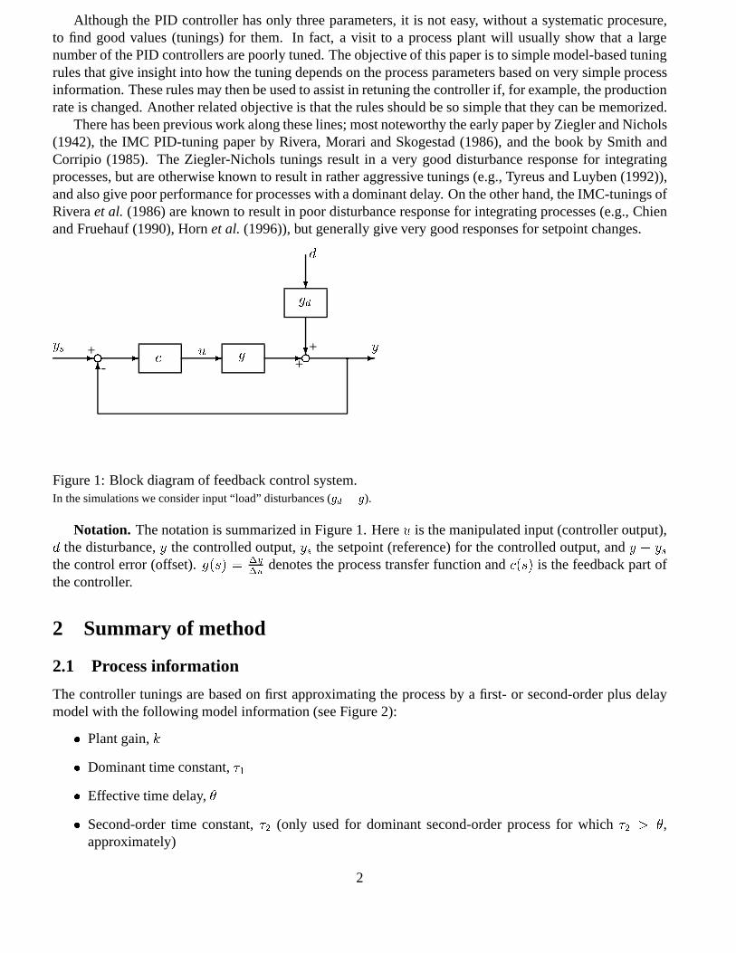
Figure 1: Block diagram of feedback control system.In the simulations we consider input “load” disturbances (gd = g).
Notation. The notation is summarized in Figure 1. Hereu is the manipulated input (controller output),d the disturbance,y the controlled output,ys the setpoint (reference) for the controlled output, andy � ysthe control error (offset).g(s) = �y
�udenotes the process transfer function andc(s) is the feedback part of
the controller.
2 Summary of method
2.1 Process information
The controller tunings are based on first approximating the process by a first- or second-order plus delaymodel with the following model information (see Figure 2):
� Plant gain,k
� Dominant time constant,�1
� Effective time delay,�
� Second-order time constant,�2 (only used for dominant second-order process for which�2 > �,approximately)
2
0 5 10 15 20 25 30 35 400
0.1
0.2
0.3
0.4
0.5
0.6
0.7
0.8
0.9
1
0 5 10 15 20 25 30 35 400
0.1
0.2
0.3
0.4
0.5
0.6
0.7
0.8
0.9
1
θ τ1
y(t)
u(t)
0.63
k = ∆ y(∞) / ∆ u
0 5 10 15 20 25 30 35 400
0.1
0.2
0.3
0.4
0.5
0.6
0.7
0.8
0.9
1
0 5 10 15 20 25 30 35 400
0.1
0.2
0.3
0.4
0.5
0.6
0.7
0.8
0.9
1
θ τ1
y(t)
u(t)
0.63
k = ∆ y(∞) / ∆ u
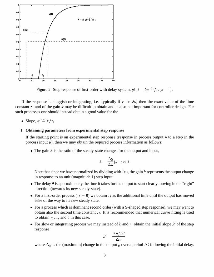
Figure 2: Step response of first-order with delay system,g(s) = ke��s=(�1s + 1).
If the response is sluggish or integrating, i.e. typically if�1 > 8�, then the exact value of the timeconstant�1 and of the gaink may be difficult to obtain and is also not important for controller design. Forsuch processes one should instead obtain a good value for the
� Slope,k0 def= k=�1
1. Obtaining parameters from experimental step response
If the starting point is an experimental step response (response in process outputy to a step in theprocess inputu), then we may obtain the required process information as follows:
� The gaink is the ratio of the steady-state changes for the output and input,
k =�y
�u(t!1)
Note that since we have normalized by dividing with�u, the gaink represents the output changein response to an unit (magnitude 1) step input.
� The delay� is approximately the time it takes for the output to start clearly moving in the “right”direction (towards its new steady-state).
� For a first-order process (�2 = 0) we obtain�1 as the additional time until the output has moved63% of the way to its new steady state.
� For a process which is dominant second order (with a S-shaped step response), we may want toobtain also the second time constant�2. It is recommended that numerical curve fitting is usedto obtain�1, �2 and� in this case.
� For slow or integrating process we may instead ofk and�1 obtain the initial slopek0 of the stepresponse
k0 =�y=�t
�u
where�y is the (maximum) change in the outputy over a period�t following the initial delay.
3
τ1 + θ
A0
A1
k
τ1+θ = (A
0/k)
τ1 = 2.71 (A
1/k)
τ1 + θ
A0
A1
k
τ1+θ = (A
0/k)
τ1 = 2.71 (A
1/k)
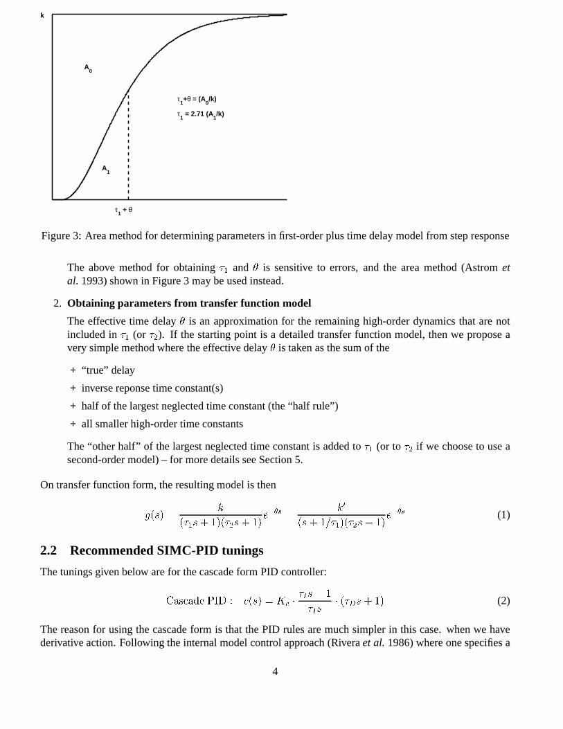
Figure 3: Area method for determining parameters in first-order plus time delay model from step response
The above method for obtaining�1 and � is sensitive to errors, and the area method (Astrometal. 1993) shown in Figure 3 may be used instead.
2. Obtaining parameters from transfer function model
The effective time delay� is an approximation for the remaining high-order dynamics that are notincluded in�1 (or �2). If the starting point is a detailed transfer function model, then we propose avery simple method where the effective delay� is taken as the sum of the
+ “true” delay
+ inverse reponse time constant(s)
+ half of the largest neglected time constant (the “half rule”)
+ all smaller high-order time constants
The “other half” of the largest neglected time constant is added to�1 (or to �2 if we choose to use asecond-order model) – for more details see Section 5.
On transfer function form, the resulting model is then
g(s) =k
(�1s+ 1)(�2s+ 1)e��s =
k0
(s+ 1=�1)(�2s+ 1)e��s (1)
2.2 Recommended SIMC-PID tunings
The tunings given below are for the cascade form PID controller:
Cascade PID : c(s) = Kc � �Is+ 1
�Is� (�Ds+ 1) (2)
The reason for using the cascade form is that the PID rules are much simpler in this case. when we havederivative action. Following the internal model control approach (Riveraet al.1986) where one specifies a
4
first-order closed-loop response with time constant�c, the following SIMC tunings1 are recommended forthe process in (1) (see derivation in Section 3):
Kc =1
k
�1�c + �
=1
k01
�c + �(3)
�I = minf�1; 4
k0 Kcg = minf�1; 4(�c + �)g (4)
�D = �2 (5)
where�� < �c <1 is the tuning parameter. The optimal value of�c is determined by a trade-off between
1. fast speed of response and good disturbance rejection (which are favored by a small value of�c), and
2. stability, robustness issues and small input usage (which are favored by a large value of�c).
For robust tunings it is recommended to use�c � �.The original IMC tuning rules (Riveraet al.1986) yield�I = �1, that is, the integral time is selected so
as to exactly cancel the dynamics correpsonding to the dominant (first-order) time constant�1. However,this gives a very sluggish response to input (load) disturbances for “slow” (�1 large) or integrating processes(Chien and Fruehauf 1990). Therefore, for such processes it is suggested to use a smaller integral time, andthe recommended value�I = 4
k0Kcjust avoids the slow oscillations that would otherwise result by using
“too much” integral action for such a process.Derivative action is primarily recommended for processes with dominant second order dynamics (with
�2 > �). Here the derivative time is selected so as to cancel the second-largest process time constant. Inaddition, derivative action is often needed to stabilize unstable processes, but such processes are not coveredhere.
2.3 Tuning for fast response with good robustness
The main limitation on achieving a fast closed-loop response is the time delay. Selecting the desired re-sponse time equal to the time delay,
SIMC : �c = � (6)
gives a reasonably fast response with moderate input usage and good robustness margins, and results in thefollowing SIMC-PID tunings which may be easily memorized:
Kc =0:5
k
�1�=
0:5
k01
�(7)
�I = minf�1; 8�g (8)
�D = �2 (9)
Two common robustness measures are the gain margin (GM) and phase margin (PM). Typical minimumrequirements are GM> 1:7 and PM> 30o (Seborget al. 1989), but for most control loops in the processindustries larger margins are recommended. Alternative robustness measures are the peak valueMs of thesensitivity functionS = 1=(1 + gc), and the peak valueMt of the complementary sensitivity, for whichsmall values are desirable. For example,Ms < 2 guarantees GM>2 and PM> 29:0o.
With the SIMC PID-tunings in (7)-(9) the gain margin is typically above 3, the phase margin is about50o � 60o, andMs is 1.7 or less (Holm and Butler 1998). Specifically, with�I = �1 the system always
1The S in “SIMC” denotes Skogestad, Simple or Super – pick your choice.
5

has a gain margin (GM) of 3.14, a phase margin (PM) of61:4o, Ms = 1:59, and a maximum allowed timedelay error of2:14� i.e., the tunings provide time delay error robustness in excess of 200% (see Table 1).As expected, the robustness margins are somewhat poorer for “sluggish” processes, where we in orderto improve the disturbance response use�I = 8�. For example, for an integrating process the suggestedtunings give a a gain margin of 2.96, a phase margin of46:9o, and a maximum allowed time delay error of1:49�.
Processg(s) k�1s+1
e��s k0
se��s
Controller gain,Kc0:5k
�1�
0:5k0
1�
Integral time,�I �1 8�Gain margin (GM) 3.14 2.96Phase margin (PM) 61.4o 46.9o
Allowed time delay error,��=� 2.14 1.59Sensitivity peak,Ms 1.59 1.70Complementary sensitivity peak,Mt 1.00 1.30Phase crossover frequency,!180 � � 1.57 1.49Gain crossover frequency,!c � � 0.50 0.51
Table 1: Robustness margins for first-order and integrating delay process using SIMC-tunings in (7) and (8)(�c = �). The same margins apply to second-order processes if we choose�D = �2.
Derivation: For the first-order delay process with�I = �1 the resulting loop transfer function isL(s) = gc = 0:5
�se��s. The
frequency!180 where the phase ofL is�180o is then6 L = �!180���
2= �� ) w180 =
�
2
1
�. The gain ofL as a function
of frequency is0:5=�! and by evaluating the gain at the frequency!180 we find that GM= 1=jL(j!180)j = � = 3:14. Similarly,
we can show that the frequency!c wherejLj = 1 is!c = 0:5=� og we find that PM= � � 6 L(j!c) = �=2� 0:5[rad] = 61:4o.
The maximum allowed time delay error is then�� = PM=!C = (� � 1)� = 2:14�.
These good margins come at the expense of a somewhat more sluggish time response compared to thatwhich can be achieved with more aggressive tunings. Note that for the case with�I = �1, increasingKc bya factor of 2 (corresponding to choosing�c = 0), reduces PM from 61o to 33o and reduces GM from 3.14 to1.57, which are rather poor robustness margins. Thus, to maintain resonable robustness, the controller gainshould be at most a factor of 2 larger than the value given in (7).
2.4 Tuning for slow response
In many cases the above choice�c = � may be unnecessary “aggressive” and we may want to increase�cor equivalently decreaseKc. In particular, this may be the case for processes with a small (effective) timedelay, for example, a pure first-order process. More generally, there are cases where we want to use as littlecontrol as possible, that is, we want a slow or smooth response. However, there is usally some performancerequirements in terms of the allowed output variation, and this gives a minimum controller gain needed toachieve satisfactory disturbance rejection. For example, for the case of input “load” disturbances we mustapproximately require that (see (37) below):
Kc � duymax
(10)
Hereymax is the allowed output error (y � ys), anddu is the magnitude of the input “load” disturbance. Asexpected, tight control withymax small requiresKc large, as does a large disturbances withdu large.
6
After deciding on a reasonable value forKc, one may from (3) back-calculate the corresponding valueof �c. For cases where the integral time is not equal to�1 one may then modify the integral time accordingto (4).
If the “minimum” controller gain given by (10) is larger than the “maximum” the controller gain givenin (7), then the process is not controllable – at least not with PID control with reasonably robust tunings. Inwords, the speed of response required for disturbance rejection is faster than what can be achieved with thegiven time delay.
Example. Consider a second-order with delay process with time constants�1 = 6 and�2 = 1:2, and timedelay� = 0:25:
g(s) = 4e�0:25s
(6s+ 1)(1:2s+ 1)(11)
The requirements is that the output deviation should be less thanymax = 1 in response to a load disturbancedu = 0:5. It is also desirable that the input usage is as smooth as possible.
Tuning for fast response. With �c = � = 0:25 the recommended tunings (7)-(9) for a cascade formPID controller are
Kc =0:5
k
�1�= 3; �I = 8� = 2; �D = �2 = 1:2 (12)
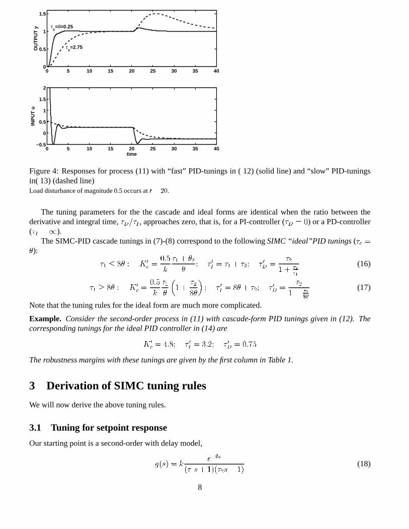
The load disturbance response in Figure 4 is much better than the requirement, with a output deviation inresponse to the load disturbance of less than 0.1. However, the input has some overshoot and oscillations.
Tuning for slow response.The above response is unecessary fast. To reject the disturbance we needa minimum gain, which from (10) is approximatelyKc =
duymax
= 0:51
= 0:5 (corresponding to�c = 2:75),and the resulting PID tunings are
Kc = 0:5; �I = �1 = 6; �D = �2 = 1:2 (13)
The load disturbance response in Figure 4 has an output deviationy � ys of about1:5� 1 = 0:5 which iswell below 1, and the input is smooth with no overshoot or oscillations. Thus, this tuning is preferred inpractice.
Remark: We may reduceKc further below 0.5 and still achieve an output deviation less than 1. Thereason why (10) is not tight, is that (1) the expression is derived for sinusoidal disturbances whereas we con-sider a step disturbance, and (2) the derivative time is quite close to the integral time so that the controllergain as a function of frequency does not come down to its asymptotic value ofKc.
2.5 Ideal PID controller
The above tunings (Kc; �I ; �D) are for the cascade form PID controller in (2). To derive the correspondingtunings for the “ideal” PID controller
Ideal PID : c0(s) = K 0c
1 +
1
� 0Is+ � 0Ds
!=
K 0c
� 0Is
�� 0I�
0Ds
2 + (� 0I + � 0D)s+ 1�
(14)
we use the formulas
K 0c = Kc
�1 +
�D�I
�; � 0I = �I
�1 +
�D�I
�; � 0D =
�D1 + �D
�I
(15)
Note that it isnotalways possible to do the reverse and obtain cascade tunings from the ideal tunings. Thisis because the ideal form is slightly more general as it also allows for complex zeros in the controller. Thus,if we want to derive PID-tunings for a second-order oscillatory process which has complex poles, then weshould start directly with the ideal PID controller.
7
0 5 10 15 20 25 30 35 400
0.5
1
1.5
OU
TP
UT
y
τc=2.75
0 5 10 15 20 25 30 35 40−0.5
0
0.5
1
1.5
2
INP
UT
u
time
τc=θ=0.25
0 5 10 15 20 25 30 35 400
0.5
1
1.5
OU
TP
UT
y
τc=2.75
0 5 10 15 20 25 30 35 40−0.5
0
0.5
1
1.5
2
INP
UT
u
time
τc=θ=0.25
Figure 4: Responses for process (11) with “fast” PID-tunings in ( 12) (solid line) and “slow” PID-tuningsin( 13) (dashed line)Load disturbance of magnitude 0.5 occurs att = 20.
The tuning parameters for the the cascade and ideal forms are identical when the ratio between thederivative and integral time,�D=�I , approaches zero, that is, for a PI-controller (�D = 0) or a PD-controller(�I =1).
The SIMC-PID cascade tunings in (7)-(8) correspond to the followingSIMC “ideal”PID tunings (�c =�):
�1 � 8� : K 0c =
0:5
k
�1 + �2�
; � 0I = �1 + �2; � 0D =�2
1 + �2�1
(16)
�1 � 8� : K 0c =
0:5
k
�1�
�1 +
�28�
�; � 0I = 8� + �2; � 0D =
�21 + �2
8�
(17)
Note that the tuning rules for the ideal form are much more complicated.
Example. Consider the second-order process in (11) with cascade-form PID tunings given in (12). Thecorresponding tunings for the ideal PID controller in (14) are
K 0c = 4:8; � 0I = 3:2; � 0D = 0:75
The robustness margins with these tunings are given by the first column in Table 1.
3 Derivation of SIMC tuning rules
We will now derive the above tuning rules.
3.1 Tuning for setpoint response
Our starting point is a second-order with delay model,
g(s) = ke��s
(�1s+ 1)(�2s+ 1)(18)
8
for which we want to derive analytical PID-settings. We use thedirect synthesisapproach of Riveraet al.(1986) where we specify the desired setpoint response. Under feedback control the closed-loop setpointresponse of the system in Figure1 is
y
ys=
gc
gc+ 1(19)
wherec is the feedback controller, and we have assumed that the measurement of the outputy is perfect.Following Riveraet al. (1986), we specify that we, after the delay, desire a simple first-order response
y
ys
!desired
=1
�cs+ 1e��s (20)
We have kept the delay in the “desired” response because it is unavoidable.�c is the desired closed-looptime constant, and is the sole tuning parameter for the controller. Combining (19) and (20) and solving withrespect to the controller gives a “Smith Predictor” controller (Smith 1957):
c(s) =(�1s+ 1)(�2s+ 1)
k
1
(�cs+ 1� e��s)(21)
To get a PID-controller we introduce in (21) the follwing first-order Taylor approximation for the delay
e��s � 1� �s (22)
and derive
c(s) =(�1s+ 1)(�2s + 1)
k
1
(�c + �)s(23)
which is a cascade form PID-controller (2) with
Kc =1
k
�1�c + �
; �I = �1; �D = �2 (24)
Alternative approximations of the delay
1. We may instead of (22) use the more exact 1st order Pade approximation,
e��s =e��=2s
e��=2s� � �
2s+ 1
�2s+ 1
With the choice�c = � this results in the same PID-controller (23) found above, but in addition weget a term
�2s+ 1
0:5 �2s+ 1
(25)
which may be viewed as an additional derivative term which is effective over only a very small range,and increases the controller gain by a factor 2 at high frequencies. Simulations show that performanceis only slightly improved by adding this term (at least with the choice�c = �; see Figure 5)), and thusdoes not justify the increased complexity of the controller.
2. Original IMC PID tunings for first-order with delay process. Riveraet al. (1986) introducedthe Pade approximation in the process itself, before deriving the controller. By specifying a closed-loop responsey=ys = �(�=2)s+1
"s+1(note that�c is denoted" in their notation) and choosing" = 2�,
their resulting “(unimproved) IMC PI-tunings” for a first-order with delay process are identical to the
9

tunings (24) just derived. They also propose some variations. One is the “improved IMC PI-tuning”where the integral time is changed from�1 to �1 + �=2:
IMC PI : Kc =1
k
�1 + �=2
"; �I = �1 + �=2 (26)
with " � 1:7�. This improvement has some effect for dominant time delay processes (with�1=�small), but it is minor and probably does not justify the added complication in the rule.
Riveraet al. (1986) also propose for a first-order with delay process to use an additional derivativeterm with time constant�=2 resulting in the “IMC PID-tunings”:
IMC cascade � PID : Kc =1
k
�1"+ �=2
; �I = �1; �D =�
2(27)
with " � 0:8�. With their recommended value" = 0:8� (tight control) this gives some improvementwith less overshoot in the setpoint response, but the load disturbance response is almost unchanged.For larger values of" (more robust tuning corresponding to the SIMC-rules), there is very littleimprovement also in the setpoint response; see Figure 5.
0 5 10 15 20 25 30 35 400
0.2
0.4
0.6
0.8
1
1.2
1.4
t/θ
OU
TP
UT
y
Kc = (0.5 / k ) ⋅ (τ
1 / θ )
τI = τ
1
τD=0
τD=θ/2
0 5 10 15 20 25 30 35 400
0.2
0.4
0.6
0.8
1
1.2
1.4
t/θ
OU
TP
UT
y
Kc = (0.5 / k ) ⋅ (τ
1 / θ )
τI = τ
1
τD=0
τD=θ/2
Figure 5: Introduction of derivative action (solid line) has only a minor effect for first-order with delayprocess,g(s) = ke��s=(�1 + 1)Note: Controller gain corresponds to�c = � in (24) and" = 2� in (27)Load disturbance of magnitude 0.5 occurs att = 20.
In summary, the tunings proposed in this paper are similar to the IMC-tunings of Riveraet al. (1986).Riveraet al. (1986) proposed some modifications to improve the response, which have only a minor effect,and do not seem worthwhile. However, for a process with�1=� large, there is a significant scope forimprovement when it comes to disturbance rejection (Chien and Fruehauf 1990). This is discussed next.
3.2 Modifying the integral term for improved disturbance rejection
Above we derived PI- and PID tunings based on considering thesetpointresponse. We found that we shouldeffectively cancel the first order dynamics of the process by selecting the integral time�I = �1. This is a
10

robust setting which results in very good responses when it comes to setpoint changes and disturbancesoccuring directly at the processoutput. However, it is well known that for processes where�1 is “large”(e.g. an integrating processes), this choice results in a long settling time forinput “load” disturbances(Chien and Fruehauf 1990). The reason is that the controller cancels the process dynamics, whereas for adisturbance occuring at the input we actually want to keep the dynamics. To improve the load disturbanceresponse we therefore want to reduce the integral time. However, we must not reduce the integral timetoo much, because otherwise we will encounter slow oscillations caused by almost having two integratorsin series (one from the slow dynamics in the process and one from the controller). This is illustrated inFigure 6 for a “slow” process with�1 = 30:
� �I = �1 = 30 (IMC) gives slow settling for a load disturbance.
� �I = 8� = 8 (SIMC) gives faster settling.
� �I = 4 gives even faster settling, but the setpoint response (and robustness) is poorer.
� �I = 2 gives poor response with oscillations.
0 10 20 30 40 50 600
0.2
0.4
0.6
0.8
1
1.2
1.4
1.6
1.8
time
τI=30
8
4
2
τI=2
8
4
30y
s=
y(t)
0 10 20 30 40 50 600
0.2
0.4
0.6
0.8
1
1.2
1.4
1.6
1.8
time
τI=30
8
4
2
τI=2
8
4
30y
s=
y(t)
Figure 6: Effect of changing the integral time�I for PI-control of “slow” processg(s) = e�s=(30s + 1)with Kc = 15.Load disturbance of magnitude 10 occurs att = 20.
A good trade-off between disturbance response and robustness is obtained by selecting the integral timesuch that we just avoid the oscillations (�I = 8� in the above example). Let us analyze this in more detail.First, note that these “slow” oscillations have a different origin and occur at a lower frequency than theusual fast oscillations which occur at about the frequency of the delay,1=�. Because of this, we neglect thedelay in the model when we analyze the slow oscillations. The process model then becomes
g(s) = ke��s
�1s+ 1� k
1
�1s+ 1� k
�1s=
k0
s
where the second approximation applies since the resulting frequency of oscillations! is such that(�1!)2
is much larger than 1 (see footnote). With a PI controllerc = Kc
�1 + 1
�Is�
the closed-loop characetristic
11

equation1 + gc then becomes�I
k0KCs2 + �Is+ 1
which is on standard second-order form� 20 s2 + 2�0�s+ 1 with
�0 =
s�I
k0 Kc; � =
1
2
qk0 Kc �I (28)
To avoid slow oscillations we must have a damping coefficient� � 1. Of course, some oscillations may betolerated, but nevertheless a good starting value is to have� = 1 (see also Marlin (1995) page 588), whichgives
Kc�I = 4=k0 (29)
or equivalently
�I =4
k0Kc
(30)
which is the value recommended in (4). The choiceKc =0:5k0
1�
in (7) gives�I = 8� as given in (8). For afirst-order with delay process this gives a gain margin better than 2.96 and a phase margin better than 46.9o;see Table 1.
We get slow oscillations if the product of the controller gainKc and the integral time�I is reducedcompared to the value given in (29). What is the periodP of these oscillations? From a standard analysisof second-order systems, we have that (e.g. Seborget al. (1989) page 118)
P =2�p1� �2
�0 > 2��0 = 2�
s�I
k0Kc
(31)
where the inequality applies since the presence of oscillations requires� � 1. With the suggested tuning�I = 4=k0Kc (30) this gives
P > � � �I (32)
Thus, the “slow” oscillations which result byreducingthe controller gain have a period larger than 3 timesthe integral time.2. On the other hand, the “usual” fast oscillations that appear byincreasingthe controllergain have a period of 6 times the delay. This is illustrated in Figure 7 for a “slow” process with�1 = 30,� = 1 and integral time�I = 4:
� Kc = 15 gives no detectable oscillations.
� Increasing the controller gain (Kc = 30) gives fast oscillations with a period of about 6 (about 6 timesthe delay).
� Decreasing the controller gain (Kc = 3) gives slow oscillations with a period of about 30 (larger than3 times the integral time).
2The corresponding normalized frequency of these slow oscillations is�1! = �1 � 2�=P � 2�1=�I which is larger than 2since we use�I � �1.
12

0 5 10 15 20 25 30 35 40 45 500
0.2
0.4
0.6
0.8
1
1.2
1.4
1.6
1.8
2K
c=30
time
OU
TP
UT
y
Kc=15 K
c=3
0 5 10 15 20 25 30 35 40 45 500
0.2
0.4
0.6
0.8
1
1.2
1.4
1.6
1.8
2K
c=30
time
OU
TP
UT
y
Kc=15 K
c=3
Figure 7: Effect of changing the gainKc for PI-control of “slow” processg(s) = e�s=(30s+1) with �I = 4.Setpoint responses.
3.3 Lower limit on controller gain
In many practical situations we do not require very fast control, and to reduce the use of manipulatedinputs and generally make operation smoother we may want to use lower controller gains. Are there anylower limits on the controller gain? Yes, there are, and to derive this we will consider the performancerequirements for disturbance rejection.
The linear transfer fuction model with deviation variables is
y = g(s)u+ gd(s)d (33)
wheregd(s) is the disturbance transfer function model. With feedback control,u = �c(s)y, the effect of adisturbanced on the control outputy is
y = S(s)gd(s)d
whereS(s) = 1=(1 + g(s))c(s) is the sensitivity function. Letd denote the disturbance magnitude, andymax the allowed output variation. We assume that this requirement applies on a frequency-by-frequencybasis, i.e., for a sinusoidal disturbance with frequency! [rad/min] and magnituded, the resulting sinusoidaloutput should have a magnitude less thanymax. Since the sinusoidal response is mathematically obtainedby settings = j!, the requirement becomes
jy(j!)j = jS(j!)j � jgd(j!)j � d � ymax
or
j1 + g(j!)c(j!)j � jgd(j!)j � dymax
At low frequencies (i.e., within the closed-loop bandwith) we have thatjgcj � 1 and we derive the followinglower limit on the frequency-dependent controller gain
jc(j!)j � jgd(j!)j � djg(j!)j � ymax
(34)
13
At lower frequencies, where this expression applies, we effectively have “perfect control” andy � 0. From(33) the required input to reject the disturbance (i.e., achievey = 0) is ud = (gd=g)d, and we derive thefollowing alternative expression
jc(j!)j � ud(j!)
ymax
(35)
whereud(j!) is the magnitude of the input change needed to reject the disturbances andymax is the maxi-mum allowed output deviation (y � ys). By constructing a controller which just satisfies the bound (34) or(35), we obtain the “slowest” acceptable controller (this is generally not a PID controller).
For the special case of aload disturbance (distubancedu at the input) we havegd = g and the require-ment (34) becomes
c(j!) � duymax
(36)
For a P-, PI- and PID-controller the controller gainjc(j!)j has a minimum asymptotic value3 of Kc, andwe derive the following lower limit on the controller gain,
Kc � duymax
(37)
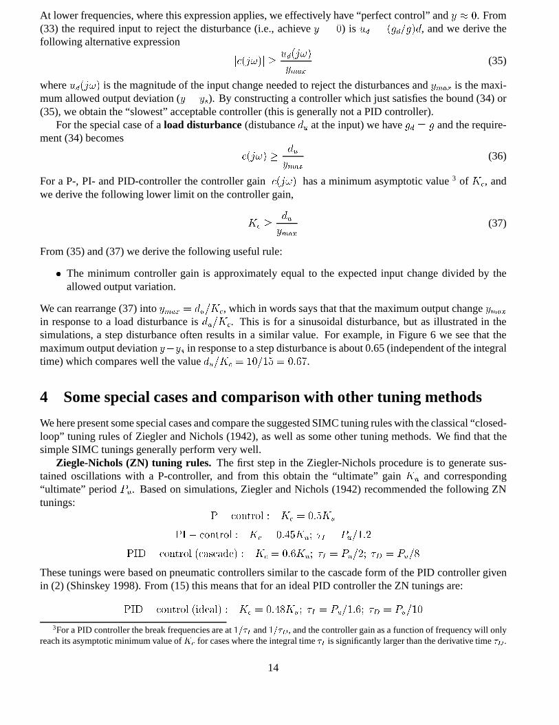
From (35) and (37) we derive the following useful rule:
� The minimum controller gain is approximately equal to the expected input change divided by theallowed output variation.
We can rearrange (37) intoymax = du=Kc, which in words says that that the maximum output changeymax
in response to a load disturbance isdu=Kc. This is for a sinusoidal disturbance, but as illustrated in thesimulations, a step disturbance often results in a similar value. For example, in Figure 6 we see that themaximum output deviationy�ys in response to a step disturbance is about 0.65 (independent of the integraltime) which compares well the valuedu=Kc = 10=15 = 0:67.
4 Some special cases and comparison with other tuning methods
We here present some special cases and compare the suggested SIMC tuning rules with the classical “closed-loop” tuning rules of Ziegler and Nichols (1942), as well as some other tuning methods. We find that thesimple SIMC tunings generally perform very well.
Ziegle-Nichols (ZN) tuning rules. The first step in the Ziegler-Nichols procedure is to generate sus-tained oscillations with a P-controller, and from this obtain the “ultimate” gainKu and corresponding“ultimate” periodPu. Based on simulations, Ziegler and Nichols (1942) recommended the following ZNtunings:
P� control : Kc = 0:5Ku
PI� control : Kc = 0:45Ku; �I = Pu=1:2
PID� control (cascade) : Kc = 0:6Ku; �I = Pu=2; �D = Pu=8
These tunings were based on pneumatic controllers similar to the cascade form of the PID controller givenin (2) (Shinskey 1998). From (15) this means that for an ideal PID controller the ZN tunings are:
PID� control (ideal) : Kc = 0:48Ku; �I = Pu=1:6; �D = Pu=10
3For a PID controller the break frequencies are at1=�I and1=�D, and the controller gain as a function of frequency will onlyreach its asymptotic minimum value ofKc for cases where the integral time�I is significantly larger than the derivative time�D .
14
Tyreus-Luyben modified ZN tuning rules. The ZN tunings were derived to give decay ratio of 1/4.This is too aggressive for most process control systems, where oscillations and overshoot is usually not de-sired at all. This lead Tyreus and Luyben (1992) to recommend the following PI-rules for more conservativeloops:
Kc = 0:313Ku; �I = 2:2Pu
Regressed analytic tuning rules.Many papers on PID control include comparisons with the tuningrules of Cohen and Coon (1953) where the tunings are given by analytical functions ofk; �1 and�. Thesetunings were also derived for a decay ratio of 1/4 and are generally too aggressive, and performance isusually poor (this is probably why it is popular to compare with them since anyoone can beat them). Later,there has been many papers along these lines, e.g. Hoet al. (1998).
Astrom PI tuning rules. Schei (1994) argued that in process control applications we usually want a ro-bust design with the highest possible attenuation of low-frequency disturbances, and suggested to maximizethe low-frequency controller gain
KI =Kc
�I(38)
subject to given robustness constraints onMs andMt. Astromet al. (1998) showed how to formulate thisas a convex optimization problem for the case with PI control and a constraint onMs. The value of thetuning parameterMs is typically between 1.4 (robust tuning) to 2 (more agressive tuning). To improve thesetpoint performance Astromet al. (1998) use a “two degrees of freedom controller” where they use only afractionb of the propotional action on the setpoint, but we do not use this here (i.e., we setb = 1).
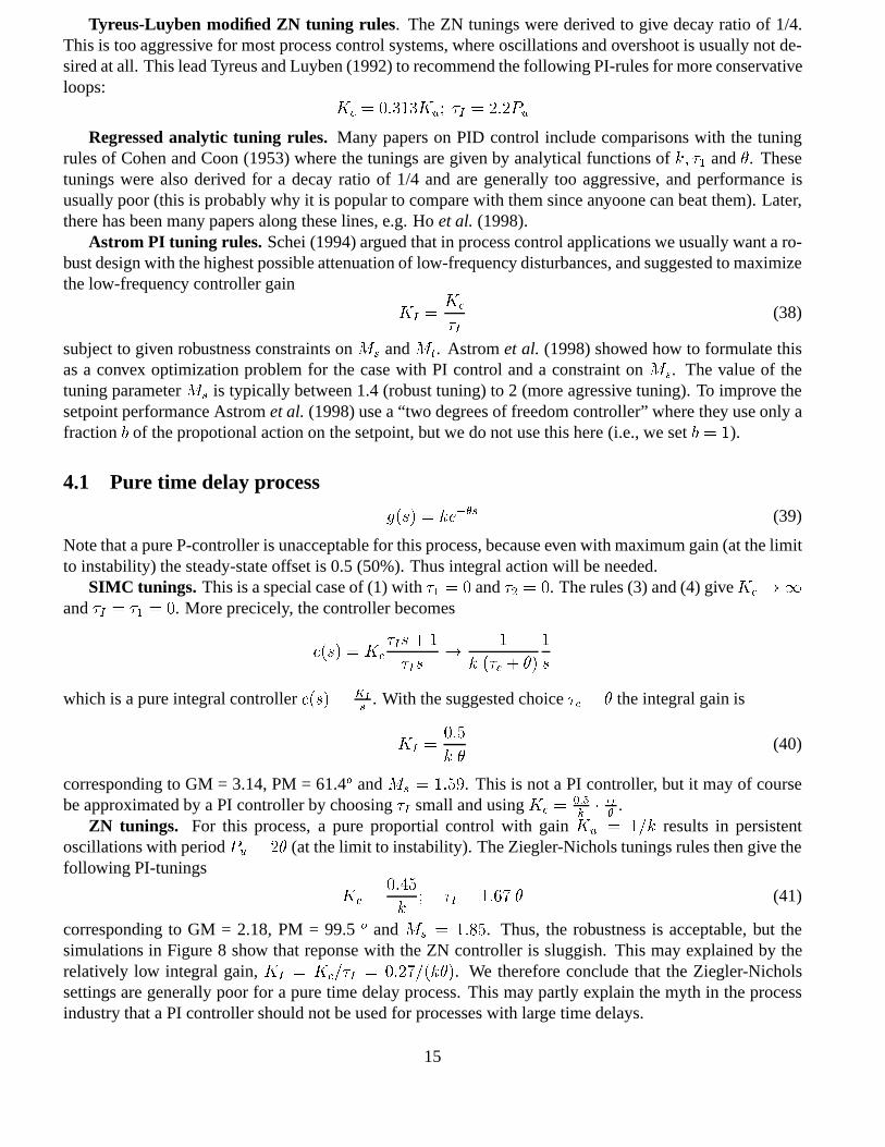
4.1 Pure time delay process
g(s) = ke��s (39)
Note that a pure P-controller is unacceptable for this process, because even with maximum gain (at the limitto instability) the steady-state offset is 0.5 (50%). Thus integral action will be needed.
SIMC tunings. This is a special case of (1) with�1 = 0 and�2 = 0. The rules (3) and (4) giveKc !1and�I = �1 = 0. More precicely, the controller becomes
c(s) = Kc�Is+ 1
�Is! 1
k (�c + �)
1
s
which is a pure integral controllerc(s) = KI
s. With the suggested choice�c = � the integral gain is
KI =0:5
k �(40)
corresponding to GM = 3.14, PM = 61.4o andMs = 1:59. This is not a PI controller, but it may of coursebe approximated by a PI controller by choosing�I small and usingKc =
0:5k� �I�
.ZN tunings. For this process, a pure proportial control with gainKu = 1=k results in persistent
oscillations with periodPu = 2� (at the limit to instability). The Ziegler-Nichols tunings rules then give thefollowing PI-tunings
Kc =0:45
k; �I = 1:67 � (41)
corresponding to GM = 2.18, PM = 99.5o andMs = 1:85. Thus, the robustness is acceptable, but thesimulations in Figure 8 show that reponse with the ZN controller is sluggish. This may explained by therelatively low integral gain,KI = Kc=�I = 0:27=(k�). We therefore conclude that the Ziegler-Nicholssettings are generally poor for a pure time delay process. This may partly explain the myth in the processindustry that a PI controller should not be used for processes with large time delays.
15
0 5 10 15 20 25 30 35 400
0.5
1
1.5
2
OU
TP
UT
y
0 5 10 15 20 25 30 35 400
0.5
1
1.5
INP
UT
u
time
Astrom
AstromSIMC
SIMC
ZN
ZN
ys=
0 5 10 15 20 25 30 35 400
0.5
1
1.5
2
OU
TP
UT
y
0 5 10 15 20 25 30 35 400
0.5
1
1.5
INP
UT
u
time
Astrom
AstromSIMC
SIMC
ZN
ZN
ys=
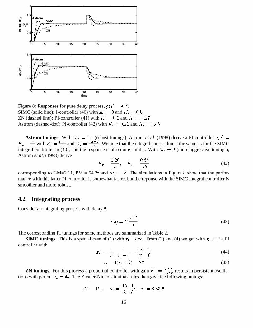
Figure 8: Responses for pure delay process,g(s) = e�s.SIMC (solid line): I-controller (40) withKc = 0 andKI = 0:5ZN (dashed line): PI-controller (41) withKc = 0:6 andKI = 0:27Astrom (dashed-dot): PI-controller (42) withKc = 0:26 andKI = 0:85
Astrom tunings. With Ms = 1:4 (robust tunings), Astromet al. (1998) derive a PI-controllerc(s) =Kc +
KI
swith Kc =
0:16k
andKI =0:4724k�
. We note that the integral part is almost the same as for the SIMCintegral controller in (40), and the response is also quite similar. WithMs = 2 (more aggressive tunings),Astromet al. (1998) derive
Kc =0:26
k; KI =
0:85
k�(42)
corresponding to GM=2.11, PM = 54.2o andMs = 2. The simulations in Figure 8 show that the perfor-mance with this latter PI controller is somewhat faster, but the reponse with the SIMC integral controller issmoother and more robust.
4.2 Integrating process
Consider an integrating process with delay�,
g(s) = k0e��s
s(43)
The corresponding PI tunings for some methods are summarized in Table 2.SIMC tunings. This is a special case of (1) with�1 ! 1. From (3) and (4) we get with�c = � a PI
controller with
Kc =1
k0� 1
�c + �=
0:5
k0� 1�
(44)
�I = 4(�c + �) = 8� (45)
ZN tunings. For this process a proportial controller with gainKu = �21k0
1�
results in persistent oscilla-tions with periodPu = 4�. The Ziegler-Nichols tunings rules then give the following tunings:
ZN� PI : Kc =0:71
k01
�; �I = 3:33 �
16

Kc � k0 � � �I=� GM PM Ms Mt
SIMC (�c = �) 0.5 8 2.96 46.9o 1.70 1.30IMC (�c = 1:7�) 0.59 1 2.66 56.2o 1.75 1.07ZN 0.71 3.33 1.86 24.8o 2.85 2.37Tyreus-Luyben 0.49 7.32 3.00 45.9o 1.70 1.33Astrom (Ms = 1:4) 0.28 7.0 5.24 47.5o 1.40 1.43Astrom (Ms = 2) 0.49 3.77 2.77 32.8o 2.00 1.81
Table 2: PI tunings for integrating process,g(s) = k0e��s=s
0 5 10 15 20 25 30 35 400
0.2
0.4
0.6
0.8
1
1.2
1.4
1.6
1.8
2
time
OU
TP
UT
y
ys=
SIMC
IMC
ZN
ZN
SIMC
0 5 10 15 20 25 30 35 400
0.2
0.4
0.6
0.8
1
1.2
1.4
1.6
1.8
2
time
OU
TP
UT
y
ys=
SIMC
IMC
ZN
ZN
SIMC
Figure 9: Responses for integrating process,g(s) = e�s=s.SIMC (solid line): PI-controller withKc = 0:5 and�I = 8.IMC (dashed line): P-controller withKc = 0:59 and�I =1.ZN (dashed-dot line): PI-controller withKc = 0:71 and�I = 3:33.
ZN� PID : Kc =0:94
k01
�; �I = 2 �; �D = �=2
The ZN tunings give (as usual) poor robustness, but as seen in Figure 9 the ZN tunings give considerablyfaster settling than the SIMC tunings for load disturbances.
The Astrom tunings withMs = 2 give responses somewhat in between SIMC and ZN.The Tyreus-Luyben modified (conservative) ZN tunings are almost indentical to the SIMC tunings for
this particular example.The IMC tunings of Riveraet al. (1986) result in a pure P-controller since�I = �1 +
�2! 1. This
P-controller is acceptable for setpoint changes, but load disturbances integrate and result in steady-stateoffset.
4.3 Integrating process with delay and lag
g(s) = k0e��s
s(�2s+ 1)(46)
17

SIMC tunings. This results in the same tunings and responses as for the process (43), but we must addderivative action to counteract the lag,
PID� cascade : Kc =1
k0� 1
�c + �; �I = 4(�c + �); �D = �2 (47)
If the time constant�2 for the lag is small, then one may approximate the process ask0 e�(�+�2)s=s andderive a PI-controller by using the rules for the integrating proces with delay in (43), but with� replaced by� + �2.
If the time constant�2 for the lag is large, such that we in effect have a double integrating process, thenthe load response is poor, and the controller needs (47) to be modified. This is discussed next.
4.4 Double integrating process
g(s) = k00e��s
s2(48)
SIMC tunings. By letting �2 ! 1 and introducingk00 = k0=�2 the PID-controller (47) obtained for theprocess (46) approaches a PD-controller with
Kc =1
k00� 1
4(�c + �)2; �D = 4(�c + �) (49)
This controller gives good setpoint responses for the process (48), but results in steady-state offset for loaddisturbances occuring at the input, see Figure 10. To remove this offset, we need to reintroduce integralaction, and as before propose to use�I = 4(�c + �). With the choice�c = � the resulting SIMC-PIDparameters are
PID� cascade : Kc =0:0625
k00� 1�2; �I = 8�; �D = 8� (50)
It should also be noted that derivative action is required in order to stabilize this process if we use integralaction in the controller.
ZN tunings can not be derived for this process because we get sustained oscillations with P-control evenwith Kc = 0.
5 The half rule: Obtaining the effective delay
In this paper we base the process information on a first-order or second-order plus delay process. Thismay seem restrictive, but more complex models can be handled by approximating the remaining high-orderdynamics by an effective delay.
The problem of obtaining the effective delay can be set up as a parameter estimation problem, forexample, by making an least squares approximation of the open-loop step response. However, our goal isto use the resulting effective delay to obtain controller tunings, so a better approach would be to find theapproximation which for a given tuning method results in the best closed-loop response (here “best” could,for example, by the in terms of the minimum integrated absolute error (IAE)).
However, our objective is not “optmality” but “simplicity”, so we choose to use a much simpler approachwhere we simply add all the “neglected” small time constants to the effective delay, except for the largestwhich we distribute evenly to the delay and the time constant using the “half method”. This extremelysimple rule has been applied to numerous examples, and leads to very good final PID tunings.
18
0 10 20 30 40 50 60 70 800
0.5
1
1.5
2
2.5
3
time
OU
TP
UT
y
SIMC−PI
SIMC−PID
0 10 20 30 40 50 60 70 800
0.5
1
1.5
2
2.5
3
time
OU
TP
UT
y
SIMC−PI
SIMC−PID
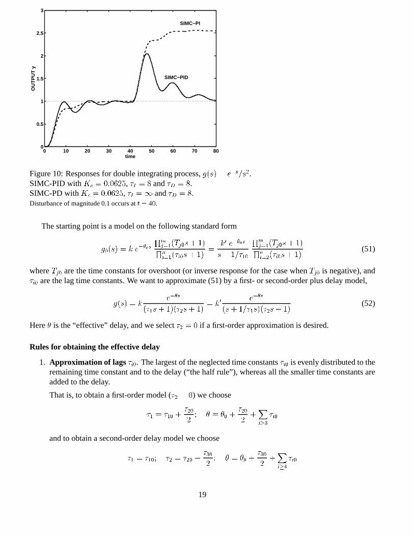
Figure 10: Responses for double integrating process,g(s) = e�s=s2.SIMC-PID withKc = 0:0625, �I = 8 and�D = 8.SIMC-PD withKc = 0:0625, �I =1 and�D = 8.Disturbance of magnitude 0.1 occurs att = 40.
The starting point is a model on the following standard form
g0(s) = k e��osQm
j=1(Tj0s+ 1)Qni=1(�i0s+ 1)
=k0 e��os
s+ 1=�10
Qmj=1(Tj0s+ 1)Qni=2(�i0s+ 1)
(51)
whereTj0 are the time constants for overshoot (or inverse response for the case whenTj0 is negative), and�i0 are the lag time constants. We want to approximate (51) by a first- or second-order plus delay model,
g(s) = ke��s
(�1s + 1)(�2s+ 1)= k0
e��s
(s+ 1=�1s)(�2s+ 1)(52)
Here� is the “effective” delay, and we select�2 = 0 if a first-order approximation is desired.
Rules for obtaining the effective delay
1. Approximation of lags �i0. The largest of the neglected time constants�i0 is evenly distributed to theremaining time constant and to the delay (“the half rule”), whereas all the smaller time constants areadded to the delay.
That is, to obtain a first-order model (�2 = 0) we choose
�1 = �10 +�202; � = �0 +
�202
+Xi�3
�i0
and to obtain a second-order delay model we choose
�1 = �10; �2 = �20 +�302; � = �0 +
�302
+Xi�4
�i0
19

2. Approximation of small or negativeTj0 as effective delay.Let �1 be the effective delay obtained sofar, and consider a numerator term withTj0 = T . ForT < �1=2 (approximately) we simply subtractT from the delay
� = �1 � T
A special case is a process with an inverse reponse (T negative), which then yields a larger effectivedelay (for example, the term(�3s+ 1) gives an effective delay� = 3)
3. Cancellation of largeTj0 by reducing time constant. ForT > �1=2 (i.e. for large positive valuesof T ) we cannot subtractT from the delay, so we instead cancel it be subtracting it from a larger timeconstant, e.g.Ts+1
�s+1� 1
(��T )s+1.
The rules are best understood by considering some examples. Simulations show that the subsequentapplication of the SIMC tuning rules result in good responses in all cases.
Example 1. The second-order process
g0(s) = 201
(10s+ 1)(s+ 1)(53)
is approximated as a first-order delay process (�2 = 0) with
�1 = 10 + 0:5 = 10:5; � = 0:5
The corresponding SIMC-PI controller tunings areKc =0:5k
�1�= 0:525 and�I = 8� = 4. The model (53)
is already second-order and the SIMC-PID tunings give�I = 10 and�D = 1, and since there is no delay wemay in theory use an infinite controller gain and achieve perfect responses (and perfect stability margins).However, in practiceKc will be limited due to uncertainty, unmodelled dynamics and limited input usage.
Example 2. The process
g0(s) = k(�0:3s+ 1)(0:08s+ 1)
(2s+ 1)(1s+ 1)(0:4s+ 1)(0:2s+ 1)(0:05s+ 1)3(54)
is approximated as a first-order delay process with
�1 = 2 + 1=2 = 2:5; � = 1=2 + 0:4 + 0:2 + 3 � 0:05 + 0:3� 0:08 = 1:47
or as a second-order delay process with
�1 = 2; �2 = 1 + 0:4=2 = 1:2; � = 0:4=2 + 0:2 + 3 � 0:05 + 0:3� 0:08 = 0:77
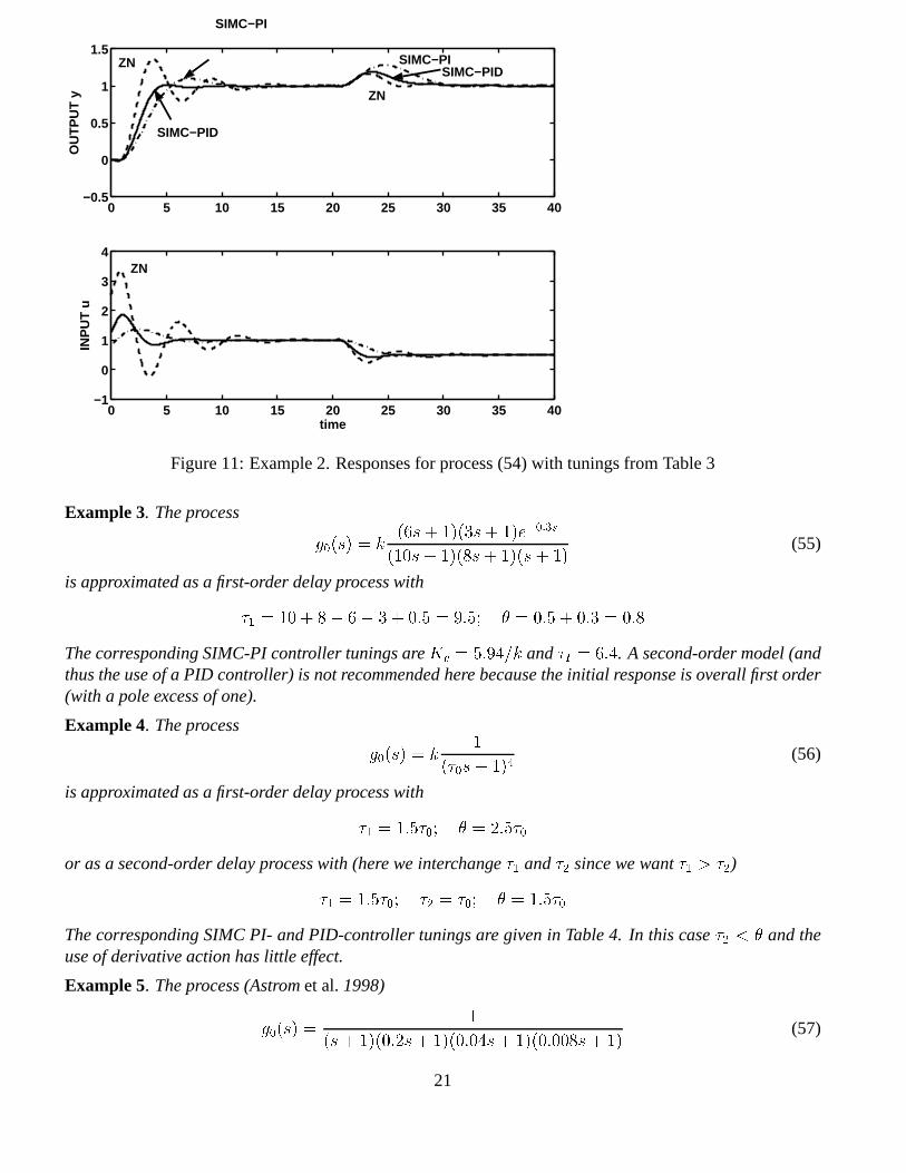
The corresponding tuning parameters for this process are given in Table 3. The responses with the SIMCtunings are very good as shown in Figure 11.
Kc � k �I �D GM PM Ms Mt
SIMC-PI 0.85 2.5 0 3.37 57.9o 1.66 1.04SIMC-PID 1.30 2 1.2 2.84 57.5o 1.74 1.05ZN-PID 2.56 2.65 0.66 1.84 30.8o 1.79 2.13
Table 3: Example 2. Tunings for process (54)
20
0 5 10 15 20 25 30 35 40−0.5
0
0.5
1
1.5
OU
TP
UT
yZN
SIMC−PID
SIMC−PI
ZN
SIMC−PID
0 5 10 15 20 25 30 35 40−1
0
1
2
3
4
INP
UT
u
time
SIMC−PI
ZN
0 5 10 15 20 25 30 35 40−0.5
0
0.5
1
1.5
OU
TP
UT
yZN
SIMC−PID
SIMC−PI
ZN
SIMC−PID
0 5 10 15 20 25 30 35 40−1
0
1
2
3
4
INP
UT
u
time
SIMC−PI
ZN
Figure 11: Example 2. Responses for process (54) with tunings from Table 3
Example 3. The process
g0(s) = k(6s+ 1)(3s+ 1)e�0:3s
(10s+ 1)(8s+ 1)(s+ 1)(55)
is approximated as a first-order delay process with
�1 = 10 + 8� 6� 3 + 0:5 = 9:5; � = 0:5 + 0:3 = 0:8
The corresponding SIMC-PI controller tunings areKc = 5:94=k and�I = 6:4. A second-order model (andthus the use of a PID controller) is not recommended here because the initial response is overall first order(with a pole excess of one).
Example 4. The process
g0(s) = k1
(�0s+ 1)4(56)
is approximated as a first-order delay process with
�1 = 1:5�0; � = 2:5�0
or as a second-order delay process with (here we interchange�1 and�2 since we want�1 > �2)
�1 = 1:5�0; �2 = �0; � = 1:5�0
The corresponding SIMC PI- and PID-controller tunings are given in Table 4. In this case�2 < � and theuse of derivative action has little effect.
Example 5. The process (Astromet al.1998)
g0(s) =1
(s+ 1)(0:2s+ 1)(0:04s+ 1)(0:008s+ 1)(57)
21

Kc � k �I=�0 �D=�0 GM PM Ms Mt
SIMC-PI 0.3 1.5 0 4.95 62.4o 1.46 1.00SIMC-PID 0.5 1.5 1 6.73 62.5o 1.43 1.00
Table 4: Example 4. Tunings for process (56)
is approximated as a first-order delay process with
�1 = 1:1; � = 0:148
or as a second-order delay process with
�1 = 1:0; �2 = 0:22; � = 0:028
The corresponding tunings are given in Table 5.As seen in Figure 12 the Ziegler-Nichols tunings almost give instability for this process, whereas the
SIMC tunings give nice closed-loop responses. A PID controller gives a significant improvement for thisprocess, which is expected since for the process is dominant second order with�2 = 0:22 much larger than� = 0:028.
Kc �I �D GM PM Ms Mt
SIMC-PI 3.72 1.1 0 6.69 51.1o 1.59 1.16ZN-PI 13.6 0.47 0 1.30 5.5o 11.3 10.9Astrom-PI(Ms = 2) 4.13 0.59 0 4.90 35.1o 2.00 1.66SIMC-PID 17.9 1.0 0.22 7.54 50.9o 1.58 1.16
Table 5: Example 5. Tunings for process (57)
Example 6. The process (Astromet al.1998)
g0(s) =(0:17s+ 1)2
s(s+ 1)2(0:028s+ 1)(58)
is approximated as an integrating process,e��s=s, with
� = 2 � 1 + 0:028� 2 � 0:17 = 1:69
or as an integrating process with lag,e��s=s(�2s+ 1), with
�2 = 1 + 1=2� 0:17 = 1:33; � = 1=2 + 0:028� 0:17 = 0:358
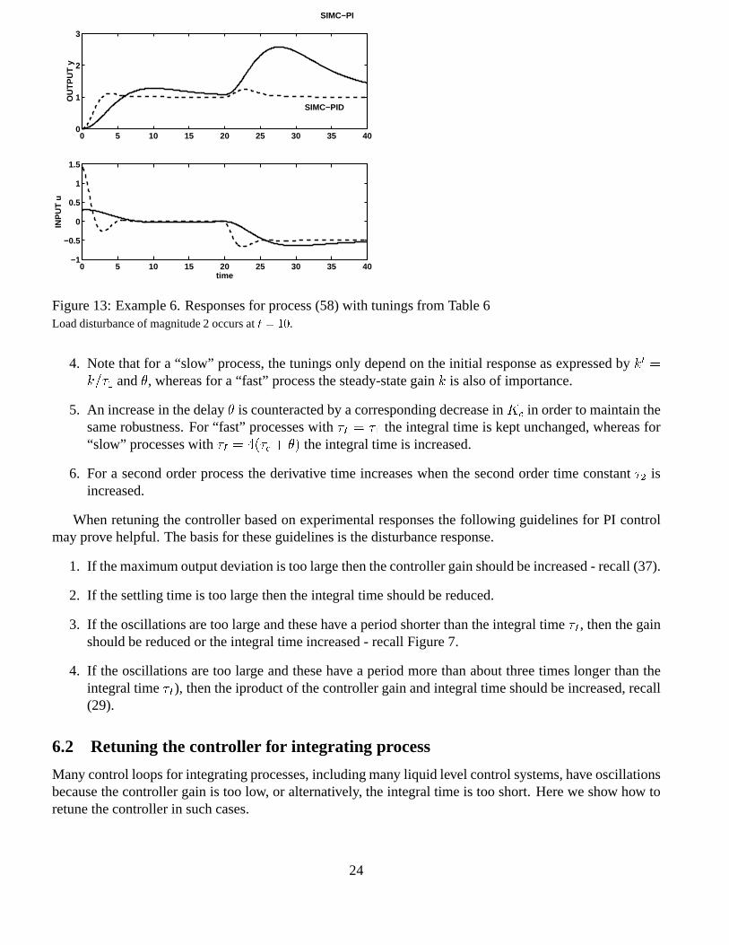
The corresponding SIMC PI- and PID-controller tunings are given in Table 6. The corresponding closed-loop responses (Figure 13) are again very good, especially for the PID-controller.
In summary, these examples illustrate that the simple SIMC tuning rules used in combination withthe simple half-rule for estimating the effective delay, result in good and robust tunings. The method forapproximating a first-order with delay model (“half rule”) and the PID tuning rules are not “optimal” in anymathematical sense, but they are simple and give surprisingly good robust performance. Furthermore, thereason for using a PID controller is simplicity, and if high performance control is desired, then one wouldnot use PID control in the first place.
A large number of additional comparisons have been performed, and there has been few cases (if any)where the proposed SIMC tuning rules perform poorly. In cases where there were large differences, theSIMC tunings could usually be improved by adjusting the tuning parameter�c.
22

0 2 4 6 8 10 12 14 16 18 200
0.2
0.4
0.6
0.8
1
1.2
1.4
1.6
1.8
2
time
OUT
PUT
y
SIMC−PI
SIMC−PI
SIMC−PID
SIMC−PID
ZN−PI
ZN−PI
Astrom−PI
Astrom−PI (Ms=2)
0 2 4 6 8 10 12 14 16 18 200
0.2
0.4
0.6
0.8
1
1.2
1.4
1.6
1.8
2
time
OUT
PUT
y
SIMC−PI
SIMC−PI
SIMC−PID
SIMC−PID
ZN−PI
ZN−PI
Astrom−PI
Astrom−PI (Ms=2)
Figure 12: Example 5. Responses for process (57) with tunings from Table 5Load disturbance of magnitude 2 occurs att = 10.
Kc �I �D GM PM Ms Mt
SIMC-PI 0.296 13.52 0 16.6 48.8o 1.48 1.29SIMC-PID 1.397 2.894 1.33 1 52.4o 1.23 1.30Astrom (Ms = 2) 0.47 7.01 0 8.2 33.1o 2.00 1.77
Table 6: Example 6. Tunings for process (58)
6 Insights
6.1 Guidelines for retuning
The tuning rules presented in this paper, see (3)-(5), give invalueable insights, for example, into how wemust change the tuning parameters in response to changes in the process model:
1. An increase in the process gaink is counteracted by reducing the controller gainKc such thatKckremains constant. (The integral time is kept constant, and the closed-loop response will remain un-changed unless there is also a change in the disturbance transfer function).
2. An increase in the process time constant�1 is counteracted by increasingKc such thatKc=�1 remainsconstant. For a “fast” process where we use�I = �1, we also need to incrase the integral time (theclosed-loop response will then remain unchanged). For a “slow” process where we use�I = 4(�c+�),we keep�I unchanged (but the closed-loop response will change somewhat in this case).
3. In many cases there is a direct correlation between the gain and the time constant such that the initialslopek0 = k=�1 remains constant. In this case we should keepKc constant. For “fast” processeswhere we use�I = �1 we should increase the integral time. For “slow” processes where we use�I = 4(�c + �) we should keep the integral time constant.
23
0 5 10 15 20 25 30 35 400
1
2
3
OU
TP
UT
y
SIMC−PID
0 5 10 15 20 25 30 35 40−1
−0.5
0
0.5
1
1.5
INP
UT
u
time
SIMC−PI
0 5 10 15 20 25 30 35 400
1
2
3
OU
TP
UT
y
SIMC−PID
0 5 10 15 20 25 30 35 40−1
−0.5
0
0.5
1
1.5
INP
UT
u
time
SIMC−PI
Figure 13: Example 6. Responses for process (58) with tunings from Table 6Load disturbance of magnitude 2 occurs att = 10.
4. Note that for a “slow” process, the tunings only depend on the initial response as expressed byk0 =k=�1 and�, whereas for a “fast” process the steady-state gaink is also of importance.
5. An increase in the delay� is counteracted by a corresponding decrease inKc in order to maintain thesame robustness. For “fast” processes with�I = �1 the integral time is kept unchanged, whereas for“slow” processes with�I = 4(�c + �) the integral time is increased.
6. For a second order process the derivative time increases when the second order time constant�2 isincreased.
When retuning the controller based on experimental responses the following guidelines for PI controlmay prove helpful. The basis for these guidelines is the disturbance response.
1. If the maximum output deviation is too large then the controller gain should be increased - recall (37).
2. If the settling time is too large then the integral time should be reduced.
3. If the oscillations are too large and these have a period shorter than the integral time�I , then the gainshould be reduced or the integral time increased - recall Figure 7.
4. If the oscillations are too large and these have a period more than about three times longer than theintegral time�I), then the iproduct of the controller gain and integral time should be increased, recall(29).
6.2 Retuning the controller for integrating process
Many control loops for integrating processes, including many liquid level control systems, have oscillationsbecause the controller gain is too low, or alternatively, the integral time is too short. Here we show how toretune the controller in such cases.
24
Consider a PI controller with (initial) tuningsKc0 and �I0 which results in “slow” oscillations withperiodP0 (by slow we mean thatP0 is larger than about3�I0). Then we most likely have an integratingprocess
g(s) = k0e��s
s
for which the product of the controller gain and integral time (Kc0�I0) is too low. Assuming�2 << 1(significant oscillations), (31) gives the following approximate expression forP0
P0 � 2��0 = 2�
s�I0 �1k0 Kc0
(59)
Thus, from (59) the product of the controller gain and integral time is approximately
Kc0�I0 = (2�)2�1k0
��I0P0
�2
To avoid oscillations (� � 1) we must from (30) require
Kc�I � 4�1k0
that is, we must require thatKc�IKc0�I0
� 1
�2��P0
�i0
�2(60)
Here1=�2 � 0:10, so we have the rule:
To avoid “slow” oscillations the product of the controller gain and integral time should beincreased by at least a factorf � 0:1(P0=�I0)
2.
The application of this simple rule should guarantee you immediate success and respect among plant oper-ators.
Example. A real industrial case study of a reboiler level control loop is shown in Figure 14. Herey is the reboiler level andu is the bottoms flow valve position. The PI tunings had been kept at theirdefault setting (Kc = �0:5 and�I = 1 min) since start-up several years ago, and resulted in an oscillatoryresponse as shown in the top part of the Figure. The control of the level (y) itself was acceptable, but thebottoms flowrate (inputu) showed large variations, and because it is the feed to the downstream columnthis caused poor temperature control in the downstream column.
From a closer analysis of the “before” response we find that the period of the slow oscillations isP0 = 0:85 h = 51 min. Since�I = 1 min, we get from the above rule we should increaseKc � �I by afactor f = 0:1 � (51)2 = 260 to avoid the oscillations. The plant personnel were somewhat sceptical toauthorize such large changes, but eventually accepted to increaseKc by a factor 7.7 and�I by a factor 24,that is,Kc�I was increased by7:7 � 24 = 185. The much improved response is shown in the “after” plot inFigure 14. There is still some minor oscillations, but these may be caused by disturbances outside the loop.In any case the control of the downstream distillation column was much improved, and the plant personnelwere very impressed by what the fresh engineer had learned in her control course in Trondheim.
7 Conclusion
The first step is to approximate the process as a first or second order process with effective delay, and thehalf rule is simple to use and gives good results. Based on this model with parametersk; �1 and�, the
25

Figure 14: Industrial case study of retuning reboiler level control system
following SIMC tunings are suggested:
Kc =1
k01
�c + �; �I = minf�1; 4(�c + �)g
If the process is second order (with�2 > �, approximately) and derivative action is acceptable we choose
Cascade PID : �D = �2
The parameter�c is the only tuning parameter, and a reasonably fast response with good robustness isobtained with�c = �. This gives robust (conservative) tunings when compared with most other tuning rules.If the response is too slow, then one may decrease the value of�c, and possibly further reduce the integraltime.
However, one may also want to increase�c to get a slower and smoother response. This results in asmaller controller gainKc, but we must require
Kc � du=ymax
(approximately) in order to keep the output deviation less thanymax in response to a load disturbance ofmagnitudedu.
Acknowledgement
Discussions with Professor David Clough from the University of Colorado at Boulder are gratefully acknowledged.
26

Simulations
In all simulations we have used a cascade PID controller with derivatice action effective over one decade (� = 0:1)and without taking the derivative of the setpoint:
u(s) = Kc�Is+ 1
�Is
�ys(s)�
�Ds+ 1
��Ds+ 1y(s)
�(61)
However, note that stability margins etc. are computed with� = 0. In most cases we use a PI controller, that is�D = 0, and the controller becomes
u(s) = Kc�Is+ 1
�Is(ys(s)� y(s)) (62)
or in the time domain
�u(t) = Kc
�(ys(t)� y(t)) +
1
�I
Z t
0(ys(�)� y(�))d�
�(63)
In the simulations a unit setpoint changeys = 1 is introduced at timet = 0, and an input “load” disturbance ofmagnitudedu = 0:5 occurs att = 20 (unless otherwise stated).
References
Astrom, K.J., H. Panagopoulos and T. Hagglund (1998). Design of PI controllers based on non-convexoptimization.Automatica34(5), 585–601.
Astrom, K.J., T. Hagglund, C.C. Hang and W.K Ho (1993). Automatic tuning and adaptation for PIDcontrollers - A survey.Control Eng. Practice1(4), 699–714.
Chien, I.L. and P.S. Fruehauf (1990). Consider IMC tuning to improve controller performance.ChemicalEngineering Progresspp. 33–41.
Cohen, G.H. and G.A. Coon (1953). Theoretical consideration of retarded control.Trans. ASME75, 827–834.
Ho, W.K., K.W. Lim and W. Xu (1998). Optimal gain and phase margin tuning for PID controllers.Auto-matica34(8), 1009–1014. See Automatica.
Holm, O. and A. Butler (1998). Robustness and performance analysis of PI and PID controller tunings.Technical report. 4th year project, Department of Chemical Engineering. Norwegian University ofScience and Technology, Trondheim. http://www.chembio.ntnu.no/users/skoge/diplom/reports/pid98-holm-butler/.
Horn, I.G., J.R. Arulandu, J. Gombas, J.G. VanAntwerp and R.D. Braatz (1996). Improved filter design ininternal model control.Ind. Eng. Chem. Res.35(10), 3437–3441.
Marlin, T.E. (1995).Process Control. McGraw-Hill.
Rivera, D.E., M. Morari and S. Skogestad (1986). Internal model control. 4. PID controller design.Ind.Eng. Chem. Res.25(1), 252–265.
Schei, T.S. (1994). Automatic tuning of PID controllers based on transfer function estimation.Automatica30(12), 1983–1989.
Seborg, D.E., T.F. Edgar and D.A. Mellichamp (1989).Process Dynamics and Control. John Wiley & Sons.
27

Shinskey, F.G. (1998). Personal communication.
Smith, C.A. and A.B. Corripio (1985).Principles and Practice of Automatic Process Control. John Wiley& Sons.
Smith, O.J. (1957). Closer control of loops with dead time.Chem. Eng. Prog.53, 217.
Tyreus, B.D. and W.L. Luyben (1992). Tuning PI controllers for integrator/dead time processes.Ind. Eng.Chem. Res.pp. 2628–2631.
Ziegler, J.G. and N.B. Nichols (1942). Optimum settings for automatic controllers.Trans. of the A.S.M.E.64, 759–768.
28