Probably Approximately Symmetric:

Fast Rigid Symmetry Detection with Global Guarantees

Simon Korman, Roee Litman, Shai Avidan and Alex Bronstein

School of Electrical Engineering, Tel Aviv University, Israel

Abstract

We present a fast algorithm for global rigid symme-

try detection with approximation guarantees. The al-

gorithm is guaranteed to find the best approximate

symmetry of a given shape, to within a user-specified

threshold, with very high probability. Our method

uses a carefully designed sampling of the transformation

space, where each transformation is efficiently evaluated

using a sub-linear algorithm. We prove that the den-

sity of the sampling depends on the total variation of

the shape, allowing us to derive formal bounds on the

algorithm’s complexity and approximation quality. We

further investigate different volumetric shape represen-

tations (in the form of truncated distance transforms),

and in such a way control the total variation of the

shape and hence the sampling density and the runtime

of the algorithm. A comprehensive set of experiments

assesses the proposed method, including an evaluation

on the eight categories of the COSEG data-set. This is

the first large-scale evaluation of any symmetry detec-

tion technique that we are aware of.

1 Introduction

Symmetry is “a distinction without a difference” in

the words of the renowned physicist and Nobel laure-

ate Frank Wilczek. Doubtlessly, symmetry along with

the related concepts of self-similarity and invariance is

an all-pervasive property of Nature and man-made art.

Engineering, architectural, and artistic designs charac-

terized by symmetry usually enjoy structural robust-

ness and efficiency, which also explains why evolution

led many biological constructions to assume symmetric

properties. Symmetry also plays an important role in

our visual perception, in particular that of beauty, and

according to modern physical theories, is incorporated

deeply into the laws of the universe itself.

Automatic detection of symmetries of a 3D geomet-

ric shape has received significant attention in computa-

tional geometry, computer graphics, and vision litera-

ture. However, despite the steady progress in the field,

the task remains computationally challenging. Existing

approaches to symmetry detection interpret symmetry

as invariance under a certain class of transformations

and they can be categorized according to several key

features. The taxonomy we present here is by no means

complete, and the reader is referred to [12, 5] for a com-

prehensive survey of symmetry detection in 3D shapes

and images.

First and foremost, symmetry is characterized by a

group of admissible transformations. While it is cus-

tomary to tacitly assume the Euclidean group (defin-

ing rigid symmetries or congruences further categorized

into reflections or involutions, rotations, and improper

rotations or roto-reflections including the former two),

more elaborate types of transformations involving uni-

form scaling (similarities), affine and projective trans-

formations, and even intrinsic symmetries have been

studied in the literature. Our main focus will be re-

stricted to rigid symmetries, though the proposed algo-

rithm and analysis can be extended to practically any

group with a finite (and reasonably small) number of

parameters, such as the affine group.

Second, symmetries can be classified as global, partial,

and local. Global symmetry is defined by a transforma-

tion that maps the whole shape onto itself. A shape

not possessing a global symmetry can still have partial

symmetries in the form of self-similar parts. Local sym-

metry usually refers to regular spatial arrangements of

a structural element into tilings and ornaments. Here,

we focus on global symmetries.

Finally, exact (perfect) and approximate (imperfect)

symmetries can be distinguished: the former map the

shape exactly to itself, whereas in case of the latter the

mapping leads to a distortion smaller than a pre-defined

threshold. Depending on the application, exact partial

symmetries can also be regarded as approximate global

ones. This work focuses on approximate symmetries.

1

arX

iv:1

403.

6637

v2 [

cs.C

G]

6 O

ct 2

014

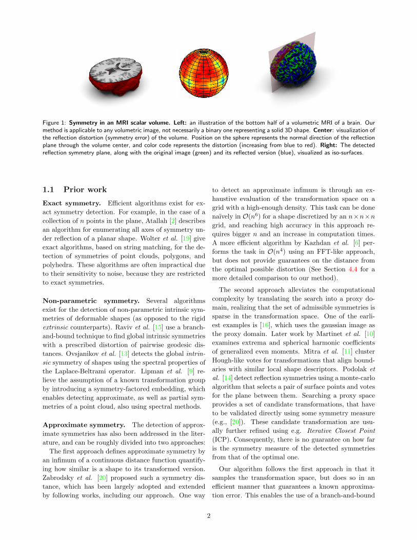
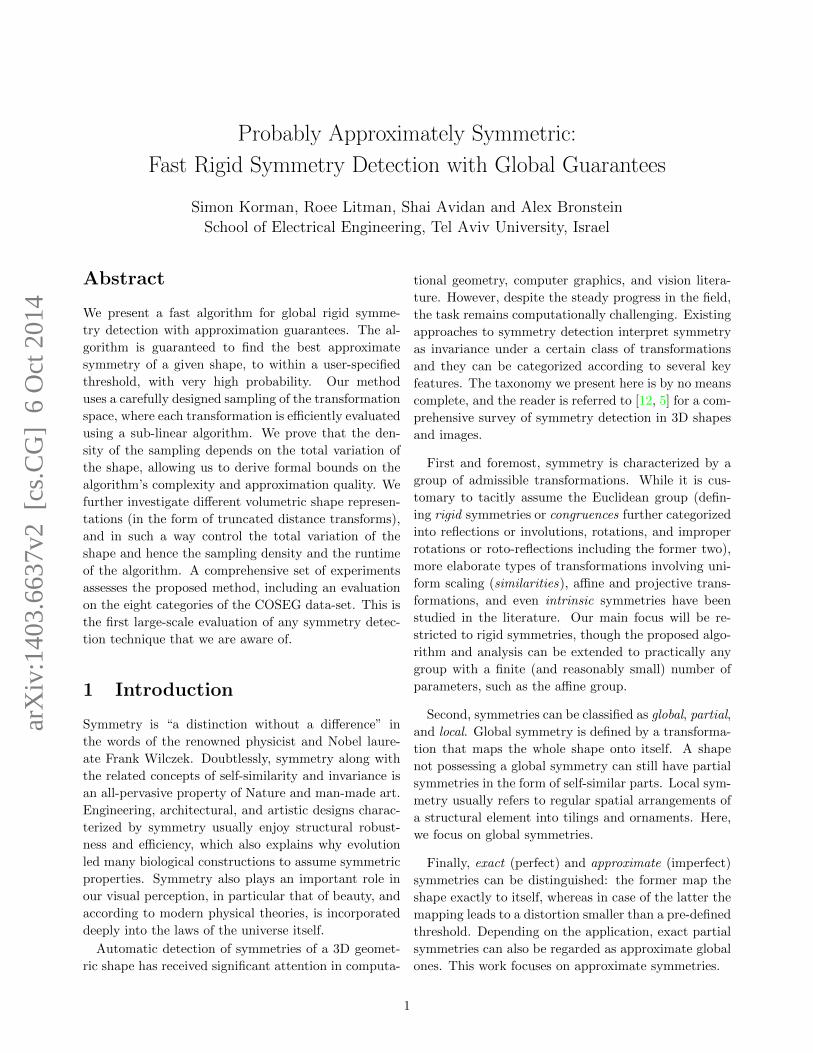
Figure 1: Symmetry in an MRI scalar volume. Left: an illustration of the bottom half of a volumetric MRI of a brain. Ourmethod is applicable to any volumetric image, not necessarily a binary one representing a solid 3D shape. Center: visualization ofthe reflection distortion (symmetry error) of the volume. Position on the sphere represents the normal direction of the reflectionplane through the volume center, and color code represents the distortion (increasing from blue to red). Right: The detectedreflection symmetry plane, along with the original image (green) and its reflected version (blue), visualized as iso-surfaces.

1.1 Prior work

Exact symmetry. Efficient algorithms exist for ex-

act symmetry detection. For example, in the case of a

collection of n points in the plane, Atallah [2] describes

an algorithm for enumerating all axes of symmetry un-

der reflection of a planar shape. Wolter et al. [19] give

exact algorithms, based on string matching, for the de-

tection of symmetries of point clouds, polygons, and

polyhedra. These algorithms are often impractical due

to their sensitivity to noise, because they are restricted

to exact symmetries.

Non-parametric symmetry. Several algorithms

exist for the detection of non-parametric intrinsic sym-

metries of deformable shapes (as opposed to the rigid

extrinsic counterparts). Raviv et al. [15] use a branch-

and-bound technique to find global intrinsic symmetries

with a prescribed distortion of pairwise geodesic dis-

tances. Ovsjanikov et al. [13] detects the global intrin-

sic symmetry of shapes using the spectral properties of

the Laplace-Beltrami operator. Lipman et al. [9] re-

lieve the assumption of a known transformation group

by introducing a symmetry-factored embedding, which

enables detecting approximate, as well as partial sym-

metries of a point cloud, also using spectral methods.

Approximate symmetry. The detection of approx-

imate symmetries has also been addressed in the liter-

ature, and can be roughly divided into two approaches:

The first approach defines approximate symmetry by

an infimum of a continuous distance function quantify-

ing how similar is a shape to its transformed version.

Zabrodsky et al. [20] proposed such a symmetry dis-

tance, which has been largely adopted and extended

by following works, including our approach. One way

to detect an approximate infimum is through an ex-

haustive evaluation of the transformation space on a

grid with a high-enough density. This task can be done

naıvely in O(n6) for a shape discretized by an n×n×ngrid, and reaching high accuracy in this approach re-

quires bigger n and an increase in computation times.

A more efficient algorithm by Kazhdan et al. [6] per-

forms the task in O(n4) using an FFT-like approach,

but does not provide guarantees on the distance from

the optimal possible distortion (See Section 4.4 for a

more detailed comparison to our method).

The second approach alleviates the computational

complexity by translating the search into a proxy do-

main, realizing that the set of admissible symmetries is

sparse in the transformation space. One of the earli-

est examples is [16], which uses the gaussian image as

the proxy domain. Later work by Martinet et al. [10]

examines extrema and spherical harmonic coefficients

of generalized even moments. Mitra et al. [11] cluster

Hough-like votes for transformations that align bound-

aries with similar local shape descriptors. Podolak et

al. [14] detect reflection symmetries using a monte-carlo

algorithm that selects a pair of surface points and votes

for the plane between them. Searching a proxy space

provides a set of candidate transformations, that have

to be validated directly using some symmetry measure

(e.g., [20]). These candidate transformation are usu-

ally further refined using e.g. Iterative Closest Point

(ICP). Consequently, there is no guarantee on how far

is the symmetry measure of the detected symmetries

from that of the optimal one.

Our algorithm follows the first approach in that it

samples the transformation space, but does so in an

efficient manner that guarantees a known approxima-

tion error. This enables the use of a branch-and-bound

2

scheme that allows to match the performance of the sec-

ond approach while maintaining approximation guaran-

tees.

Alignment methods A method related to ours is

the surface registration algorithm of [1] that uses a

clever sampling of transformation space. However, it

is not easily applicable to the problem of detecting all

approximate symmetries of a shape.

Our work follows that of [8], who proposed a fast

method for 2D affine template matching in images with

global guarantees. As opposed to their sampling den-

sity which depends on a generic image assumption (e.g.,

image smoothness), ours is determined adaptively ac-

cording to the specific shape ‘complexity’. Additionally,

we manipulate the shape representation to control the

sampling density, and hence the algorithm’s runtime.

Finally, while template matching focuses on finding a

single best transformation, our goal is to detect all such

transformations.

1.2 Contributions

We detect global rigid symmetries in volumetric rep-

resentations of 3D shapes, and introduce an algorithm

that is guaranteed, with high probability, to detect the

best symmetry within a given degree of approxima-

tion. This is inspired by the classical “probably ap-

proximately correct” (PAC) framework [17] in learning

theory (hence the title of the present paper). To the

best of our knowledge, this is the first symmetry de-

tection algorithm coming with such a guarantee. An

example output of the algorithm, detecting the bilat-

eral symmetry in a brain MRI image, can be seen in

Figure 1.

We provide a bound on the required sampling den-

sity of transformation space, which is the basis of our

algorithm. This bound depends on the desired approxi-

mation level as well as, surprisingly, on the ‘complexity’

of the specific shape, which is manifested through the

total variation of its volumetric representation. We fur-

ther show how to construct shape representations with

reduced total variation leading to reduced complexity,

and discuss the tradeoff between complexity and sensi-

tivity to noise.

A comprehensive experimental evaluation validates

that our approach is capable of detecting approximate

symmetries in a large data-set, as well as detecting all

symmetries in complicated shapes, all within state-of-

the-art execution times.

2 Approximate rigid symmetries

We start by defining our level-set based shape represen-

tation and approximate symmetry. We then bound the

sample density required to detect approximate symme-

tries with a user specified precision parameter δ. Gen-

erally speaking, although we keep all derivations in the

continuous setting, they are straightforwardly amenable

to any reasonable discretization of the volume, includ-

ing hierarchical subdivisions.

2.1 Shape representation

Let S be a three-dimensional rigid shape with the cen-

troid aligned at the origin. We represent the shape by

the 12 -sub-level set of a level set function s : R3 7→ [0, 1].

The simplest of such representations is the binary indi-

cator function of S (equalling 1 in the interior); other

representations such as truncated distance maps will be

discussed in Section 3.1. We will freely interchange be-

tween S and s referring to a shape. We will take the

radius of the shape to be the smallest scalar r such

that the function s is invariant to rotations outside the

Euclidean ball Br(0) of radius r centered at the origin,

r = infr{s(RRRxxx) = s(xxx) : xxx ∈ Br(0),RRR ∈ SO(3)}.(1)

The ball Br(0) defines the effective support of s, which

might be larger than the shape S.

We associate with the shape the total variation of s,

VS =1

VolBr

∫Br

‖∇s(xxx)‖dvol(xxx), (2)

where dvol denotes the standard volume element. When

s is not differentiable, total variation can be defined

using the weak derivative. In particular, for the case of

the indicator function VS is equal to the ratio between

the area of the boundary ∂S and the volume of the

bounding ball Br. Geometrically, total variation can

be related to the total curvature of the shape and the

amount of “features” it contains. Note that for the

case of O(3), one could have considered derivation and

integration only tangent to concentric spheres.

2.2 Rigid symmetries

Let T ∈ E(3) be a Euclidean transformation (a com-

bination of translation, rotation, and reflection). The

transformed shape TS will be represented by the indi-

cator function s(Txxx). T is said to be an exact global

symmetry of S if s(Txxx) = s(xxx). The collection of all

symmetries of S forms a group under function compo-

3

sition, which we refer to as the symmetry group of S,

denoted by Sym S. Each symmetry T ∈ Sym S defines

a collection of stationary points, {xxx = Txxx}, which is

known to be either a line or a plane. Such a line or plane

is called a symmetry axis (or plane) of the shape. The

set of symmetry axes and planes fully defines the sym-

metry group of a shape. Since translations have no sta-

tionary points, for compactly supported shapes, Sym Sis necessarily a subgroup of the orthogonal group O(3)

containing rotations and reflections around the shape’s

centroid. For this reason, we will henceforth denote the

admissible transformations as 3×3 rotation or reflection

matrices, RRR.

Exact symmetries are a mathematical idealization

rarely achieved in practice due to acquisition and rep-

resentation inaccuracies. In order to account for such

imperfections, we define the distortion

dissRRR =1

VolBr‖s−RRR−1(s)‖1 (3)

=1

VolBr

∫Br

|s(xxx)− s(RRRxxx)|dvol(xxx),

where RRR−1(s) is a short-hand notation for (s ◦RRR)(x) =

s(RRRxxx). Note that dissRRR is bounded to the interval

[0, 1], and equals zero in the case of perfect symmetry.

For solid shapes represented by indicator functions, the

distortion can be interpreted as the total amount of

mismatched volume and it coincides with the common

symmetry measure of [20]. Note that such an L1 for-

mulation is more robust to outliers compared to, e.g.,

the worst-case Hausdorff distance.

We say that RRR ∈ O(3) defines an ε-symmetry of S if

dissRRR ≤ ε, and denote by Sym εS the collection of all

ε-symmetries of S. Note that unlike their exact counter-

parts, approximate symmetries do not necessarily form

a group.

2.3 Sampling of the orthogonal group

In order to practically detect symmetries, one neces-

sarily has to work with a finite sample of the transfor-

mation space (i.e. the orthogonal group). The main

ingredient of our approach is an upper bound on the

sampling density controlled by the maximum allowed

distortion of an approximate symmetry.

We begin by defining a metric between any two trans-

formations in the space, which will be used later to de-

fine a net of transformations. The metric measures how

far apart any point in the ball Br may be mapped by

two different transformations, formally:

D(RRR1,RRR2) = max‖xxx‖≤r

‖RRR1xxx−RRR2xxx‖. (4)

Note that this distance does not depend on the shape,

but rather only on its support radius r.

A key observation is that the difference in the dis-

tortion of two transformations is upper bounded by the

product of the shape total-variation VS and the dis-

tance D between the transformations. This is formal-

ized in the following proposition, with the accompany-

ing illustration in Figure 2.

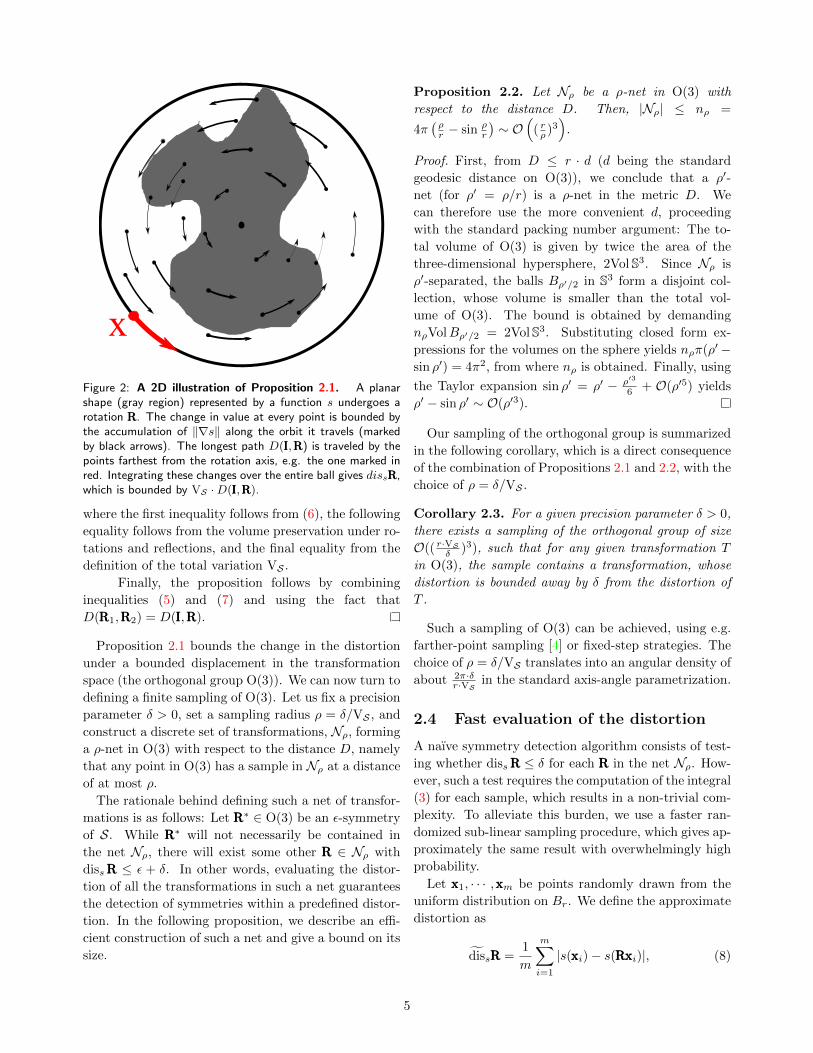
Proposition 2.1. |dissRRR1 − dissRRR2| ≤ VS ·D(RRR1,RRR2)

for any RRR1,RRR2 ∈ O(3).

Proof. First, observe that invoking the triangle inequal-

ity and using the group properties,

|dissRRR1 − dissRRR2| . . .

=1

VolBr· |‖s−RRR−11 (s)‖1 − ‖s−RRR−12 (s)‖1|

≤ 1

VolBr· ‖RRR−11 (s)−RRR−12 (s)‖1

=1

VolBr· ‖q −RRR−11 (q)‖1 = disqRRR (5)

with q = RRR−1(s) and RRR = RRR2RRR−11 . We can therefore

define a new shape Q = RRR1S with the corresponding

function q, and operate with dissRRR. Using the group

properties, it is also straightforward that D(RRR1,RRR2) =

D(III,RRR), with III being the identity transformation.

We define the flow ΦRRR : (xxx, t) → RRRtxxx, t ∈ [0, 1],

inducing the orbits C(xxx) = {RRRtxxx : xxx ∈ Br, t ∈ [0, 1]},whose length is upper-bounded by D(III,RRR) . Using the

triangle inequality,

|q(xxx)− q(RRRxxx)| = |q ◦ ΦRRR(xxx, 0)− q ◦ ΦRRR(xxx, 1)| (6)

≤∫ 1

0

‖∇(q ◦ ΦRRR(xxx, t))‖ ‖ΦRRR(xxx, t)‖dt

where ΦRRR(xxx, t) = ∂∂tΦRRR(xxx, t). We can now derive that

VolBr · disqRRR =

∫Br

|q(xxx)− q(RRRxxx)|dvol(xxx)

≤∫Br

∫ 1

0

‖∇(q ◦ ΦRRR(xxx, t))‖ ‖ΦRRR(xxx, t)‖dt dvol(xxx)

=

∫ 1

0

∫Br

‖∇(q ◦ ΦRRR(xxx, t))‖ ‖ΦRRR(xxx, t)‖dvol(ΦRRR(xxx, t)) dt

≤ D(III,RRR) ·∫Br

‖∇(q ◦ ΦRRR(xxx, t))‖dvol(ΦRRR(xxx, t))

= D(III,RRR) ·∫Br

‖∇q‖dvol(xxx) = D(III,RRR) ·VolBrVS ,(7)

4

x

Figure 2: A 2D illustration of Proposition 2.1. A planarshape (gray region) represented by a function s undergoes arotation RRR. The change in value at every point is bounded bythe accumulation of ‖∇s‖ along the orbit it travels (markedby black arrows). The longest path D(III,RRR) is traveled by thepoints farthest from the rotation axis, e.g. the one marked inred. Integrating these changes over the entire ball gives dissRRR,which is bounded by VS ·D(III,RRR).

where the first inequality follows from (6), the following

equality follows from the volume preservation under ro-

tations and reflections, and the final equality from the

definition of the total variation VS .

Finally, the proposition follows by combining

inequalities (5) and (7) and using the fact that

D(RRR1,RRR2) = D(III,RRR).

Proposition 2.1 bounds the change in the distortion

under a bounded displacement in the transformation

space (the orthogonal group O(3)). We can now turn to

defining a finite sampling of O(3). Let us fix a precision

parameter δ > 0, set a sampling radius ρ = δ/VS , and

construct a discrete set of transformations, Nρ, forming

a ρ-net in O(3) with respect to the distance D, namely

that any point in O(3) has a sample in Nρ at a distance

of at most ρ.

The rationale behind defining such a net of transfor-

mations is as follows: Let RRR∗ ∈ O(3) be an ε-symmetry

of S. While RRR∗ will not necessarily be contained in

the net Nρ, there will exist some other RRR ∈ Nρ with

dissRRR ≤ ε + δ. In other words, evaluating the distor-

tion of all the transformations in such a net guarantees

the detection of symmetries within a predefined distor-

tion. In the following proposition, we describe an effi-

cient construction of such a net and give a bound on its

size.

Proposition 2.2. Let Nρ be a ρ-net in O(3) with

respect to the distance D. Then, |Nρ| ≤ nρ =

4π(ρr − sin ρ

r

)∼ O

(( rρ )3

).

Proof. First, from D ≤ r · d (d being the standard

geodesic distance on O(3)), we conclude that a ρ′-

net (for ρ′ = ρ/r) is a ρ-net in the metric D. We

can therefore use the more convenient d, proceeding

with the standard packing number argument: The to-

tal volume of O(3) is given by twice the area of the

three-dimensional hypersphere, 2Vol S3. Since Nρ is

ρ′-separated, the balls Bρ′/2 in S3 form a disjoint col-

lection, whose volume is smaller than the total vol-

ume of O(3). The bound is obtained by demanding

nρVolBρ′/2 = 2VolS3. Substituting closed form ex-

pressions for the volumes on the sphere yields nρπ(ρ′−sin ρ′) = 4π2, from where nρ is obtained. Finally, using

the Taylor expansion sin ρ′ = ρ′ − ρ′3

6 + O(ρ′5) yields

ρ′ − sin ρ′ ∼ O(ρ′3).

Our sampling of the orthogonal group is summarized

in the following corollary, which is a direct consequence

of the combination of Propositions 2.1 and 2.2, with the

choice of ρ = δ/VS .

Corollary 2.3. For a given precision parameter δ > 0,

there exists a sampling of the orthogonal group of size

O(( r·VSδ )3), such that for any given transformation T

in O(3), the sample contains a transformation, whose

distortion is bounded away by δ from the distortion of

T .

Such a sampling of O(3) can be achieved, using e.g.

farther-point sampling [4] or fixed-step strategies. The

choice of ρ = δ/VS translates into an angular density of

about 2π·δr·VS

in the standard axis-angle parametrization.

2.4 Fast evaluation of the distortion

A naıve symmetry detection algorithm consists of test-

ing whether dissRRR ≤ δ for each RRR in the net Nρ. How-

ever, such a test requires the computation of the integral

(3) for each sample, which results in a non-trivial com-

plexity. To alleviate this burden, we use a faster ran-

domized sub-linear sampling procedure, which gives ap-

proximately the same result with overwhelmingly high

probability.

Let xxx1, · · · ,xxxm be points randomly drawn from the

uniform distribution on Br. We define the approximate

distortion as

dissRRR =1

m

m∑i=1

|s(xxxi)− s(RRRxxxi)|, (8)

5

input : Shape S represented by s; precisionparameter δ > 0; error probability p

output: Approximate symmetry RRR ∈ O(3);approximate distortion d

Construct a ρ = δ2VS

-net Nρ on O(3)

foreach RRR ∈ Nρ do

Sample mδ/2 = 2δ2 log 2

p random points from Br

Compute dissRRR = 1m

∑mi=1 |s(xxxi)− s(RRRxxxi)|

end

Return RRR with the minimal d = dissRRR

Algorithm 1: Best approximate symmetry detection.

where each of the summands is bounded on [0, 1]. Since

E{dissRRR} = dissRRR, we can use the Chernoff-Hoeffding

inequality to bound the probability P (|dissRRR−dissRRR| >ε), leading to the following

Proposition 2.4. For mε = 12ε2 log 2

p = O(ε−2 log 1p ),

|dissRRR− dissRRR| ≤ ε with probability higher than 1− p.

3 Symmetry detection algorithm

Putting the pieces together, we summarize in Algo-

rithm 1 the proposed method for detecting the best ap-

proximate symmetry. Combining the previous results,

we state the following

Theorem 3.1. The runtime complexity of Algorithm 1

is O((r · VS)3δ−5 log 1p ) and with probability 1 − p, it

holds that:

1. if d ≤ 0.5 · δ, then RRR is a δ-symmetry of S

2. if d > 1.5 · δ, then S has no δ-symmetries.

Observe that unless some elements of Nρ are re-

moved, the second condition will never happen, as the

algorithm will return a symmetry δ-close to the identity

transformation.

Algorithm 1 detects a single approximate symme-

try of S. In order to detect the entire Sym δS, we

run the algorithm sequentially, each time removing a

neighborhood of the detected transformation RRR from

Nρ. The neighborhood can be naturally defined as the

δ-component of RRR, computed by applying a flood-fill

procedure to Nρ. Alternatively, the neighborhood can

be defined as a ball of a fixed radius with respect to

input : Shape S represented by s; precisionparameter δ > 0; error probability p

output: Collection of δ-symmetries S = Sym δS

Initialize S = ∅Construct a ρ = δ

2VS-net Nρ on O(3)

while not all symmetries have been detected do

Run Algorithm 1 on Nρ to detect RRR withapproximate distortion d

if d > 1.5 · δ then stopif RRR is a rotation (and not a reflection) then

Let X be the set of n-fold symmetries alongits axis, with distortion ≤ δ(n = 2, · · · , N)

elseLet X = {RRR}

endAdd X to S and remove from Nρ a fixed-sizedneighborhood of each symmetry in X

end

Return all detected transformations RRR

Algorithm 2: Detection of all approximate symme-tries.

the standard geodesic distance on O(3). The latter ap-

proach was adopted in our experiments due to its sim-

plicity, despite the problems that may arise when using

a too small or too big radius (see Figure 3 for an illus-

tration).

Algorithm 2 summarizes the described procedure for

the detection of all approximate symmetries. When a

rotation symmetry is detected, we further investigate its

axis to find its n-fold symmetries (up to some integer

N). We report on an n-fold rotation if the distortion

of all its n members is below δ. A continuous (axial)

rotational symmetry is reported when the distortions of

all members of all n-fold rotations, n = 2, . . . , N , are

below δ.

too large radius too small radius flood-fill

Figure 3: Illustration of minima neighbourhood removal. A2D function, visualized using a heat-map. In our implemen-tation, we use a fixed-sized removal radius. Using a too largeradius may remove other minima, while a too small one leavesareas that might be detected in the next iteration. These phe-nomena may be avoided by applying a flood-fill procedure.

6

3.1 Manipulating the shape complexity

For a fixed precision δ, the complexity of our sym-

metry detection algorithm is governed by the term

(r · VS)3, which is the cube of the shape complexity

factor C = r · VS , a unit-less quantity that resembles

the isoperimetric quotient and describes the geometric

complexity of the function s representing the shape.

Through the total variation of s, C depends on the

function representing S and not directly on S itself.

This leads to the important issue of designing represen-

tation functions for shapes that minimize the computa-

tion complexity.

To this end, we suggest controlling the shape

complexity using truncated signed distance function

(TSDF) representations. The advantages of doing so

are two-fold: First, the TSDFs produce smoother shape

representations, which lead to faster running time.

Additionally, the resulting representation values have

lower variance (as a result of increased smoothness),

allowing use of tighter bounds than the one stated in

Proposition 2.4, which only assumes that the summands

are bounded but does not consider their variance.

Nevertheless, these advantages come at the cost of

the enhancement of thin structures (possibly amplify-

ing the effect of shot-noise) as well as the possible loss of

discriminativity, due to smoothing of fine details. The

effects (noise amplification and loss of discriminativity)

are studied below. Also, as part of our large-scale exper-

iment in Section 4.3, we analyze the influence of these

choices on discriminativity.

For a given (truncation) constant K, we define the

Euclidean TSDF by

dK(xxx, ∂S) = min{K,max{−K, d(xxx, ∂S)}} (9)

where d(xxx, ∂S) is the signed distance map from the

boundary ∂S of the shape S. Since d(xxx, ∂S) satisfies the

eikonal equation ‖∇d(xxx, ∂S)‖ = 1 almost everywhere,

the total variation of dK(xxx, ∂S) is bounded by

VS(dK) ≤ c ·K ·Area ∂SVolBr+K

, (10)

where c is a constant.

We construct a family of functions

sK(xxx) =1

2KdK(xxx, ∂S) +

1

2(11)

with the image in [0, 1], whose 12 -sub-level set is S. For

K = 0, s0 is simply the binary indicator function. De-

noting VSK = VS(sK) and CK = C(sK), we observe

that

CK ≤ (r +K) ·VSK ≤ (r +K)VS0 ·VolBr

VolBr+K

= C0

(r

r +K

)2

, (12)

which for K � r becomes CK ∼ O(K−2). Therefore,

from the point of view of the complexity factor alone,

it is advantageous to increase K without limits.

However, a largeK has a negative impact on the noise

resilience of the symmetry detection algorithm. To vi-

sualize this, assume that the shape is almost perfectly

symmetric, such that under a transformation RRR ∈ O(3),

s0 and s0RRR match except for on a small ball Bε resulting

from noise. Therefore, using s0, RRR has the distortion of

δ0 = dissRRR = VolBε/VolBr. Increasing K yields

δK =VolBε+KVolBr+K

=

(ε+K

r +K

)3

, (13)

which for K � r becomes δK ∼ 1, amplifying the noise

to unreasonable proportions.

The same effect also decreased the sensitivity to fine

features. Suppose two approximate symmetries R1 and

R2 maintain the shape invariant except for on small

balls Bε and B2ε, respectively. The corresponding dis-

tortions when using s0 are

δ1 =VolBεVolBr

=( εr

)3, δ2 =

VolB2ε

VolBr=

(2ε

r

)3

= 8δ1 .

That is, R2 is an order of magnitude ”worse” than

R1, which is typically an easily detectable situation.

When increasing K ,the discriminativity, viewed as

the ratio

δ2Kδ1K

=

(2ε+K

r +K

)3

/(ε+K

r +K

)3

=

(2ε+K

ε+K

)3

(14)

approaches 1 for K >> ε, meaning that features of size

K are smoothed out.

4 Experiments and applications

The code used to generate the reported results can be

downloaded from the project webpage [7].

Data-sets The main data-set we work with is the

COSEG data-set [18], which includes (among other)

190 shapes belonging to eight categories, that were orig-

inally purported for the evaluation of segmentation al-

gorithms. While the shapes were created using CAD

7

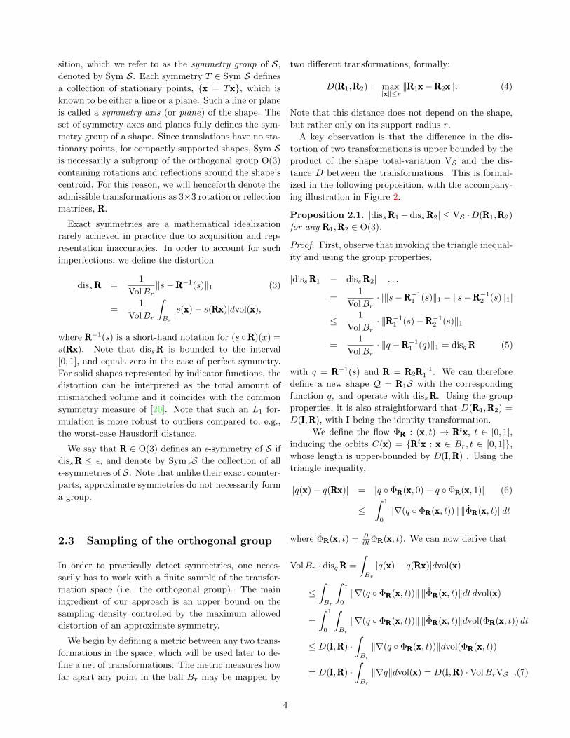
π/2 π000.10.20.30.40.50.60.70.80.9

K=0K=20K=50K=100

00

0.1

0.2

0.3

0.4

0.5

0.6

0.7

π/2 π

00

0.005

0.01

0.015

0.02

0.025

0.03

π/2 π

(a) shape (b) K=0 (binary) (c) K=20% (d) K=50% (e) K=100% (f) 1D profile along equator

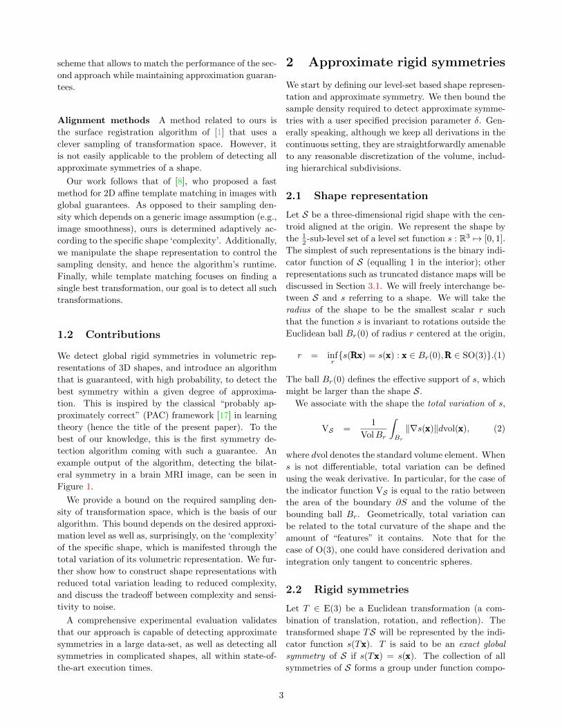
Figure 4: Distortion maps for different truncation levels. We consider only reflection symmetries in this illustration. Each rowshows one example in the following format: (a) the shape (b)-(e): distortion levels of the function sK for different truncationvalues K. Color-coding ranges from 0 (blue) to a clipped value of 0.2 (red) at each location and represents the respectivedistortion of the planar reflection symmetry, whose normal passes through the point. (f) a section of the distortion along theequator of the sphere. See text for interpretation.

tools, they are not completely synthetic in their na-

ture. Specifically, while most of the shapes have at

least one kind of symmetry, in the vast majority of the

cases the symmetry is far from being perfect, which

makes its detection challenging. We first rasterize a

randomly rotated version of each shape into a carte-

sian voxelized volume, where the maximal dimension is

taken to be 160 voxels. Since all COSEG shapes are

vertically aligned, a random rotation disables the ad-

vantage of any specific sampling location. Then, we

center the shape around its centroid and measure its

support. Finally, we pad and crop the volume to a

cube, with the side length twice the shape support ra-

dius r. This guarantees that the shape remains within

the volume under arbitrary rotations and reflections.

The final volume dimensions are around 2003.

We also created a small data-set of shapes that have

complex symmetry groups. These include the icosahe-

dron and the dodecahedron (See Figure 11 for an illus-

tration). Finding all the symmetries of such shapes is

computationally challenging. The third type of data we

use is a volumetric scalar MRI image taken from [3].

Symmetries and their notations We seek to find

approximate symmetries of different kinds. The first

kind are planar reflections, around a generally oriented

plane which passes through the centroid. We denote

such a symmetry by REFL and visualize it as a trans-

parent plane. The second kind are t-fold rotations

around an axis that passes through the centroid (where

we search for t between 2 and 20). Such a symmetry

(or a set of symmetries) includes rotation symmetries

of the set of angles {2πi/t} for i = 1, ..., t − 1. We de-

note such a symmetry by t-fold-ROT and visualize its

rotation axis in red. The third kind, axial-symmetries,

are fully-continuous rotation symmetries around some

axis. We denote these by CONT and visualize them

using a magenta colored axis.

Algorithm settings and implementation details

We represent a shape sK by applying a TSDF, where

the truncation parameter K is chosen adaptively such

that the total variation VS of the shape is approxi-

mately 3/r, as detailed in Section 4.2. When running

the main algorithm (Algorithm 2), we aim for high pre-

cision, which translates into invoking the (single sym-

metry detection) Algorithm 1 with low values of the pre-

cision parameter δ. For efficiency, we run Algorithm 1

in a branch-and-bound manner, which begins with an

initial (coarse) net defined by δ = 0.25 and iteratively

increases resolution only in ”promising” regions of the

transformation space, finally reaching the desired reso-

lution. Note that this can be done as in [8], based on our

net construction, while keeping the theoretical guaran-

8

10 20 30 40 50 60 70 80 90 1000

0.02

0.04

0.06

0.08

0.1

0.12

0.14To

tal−

Varia

tion

Truncation Parameter K [% of radius]0

0

5

10

15

20

25

30

35

40

Run

time

[sec

onds

]

RuntimeTotal-Variation (VS)AUTO Runtime medianAUTO VS median

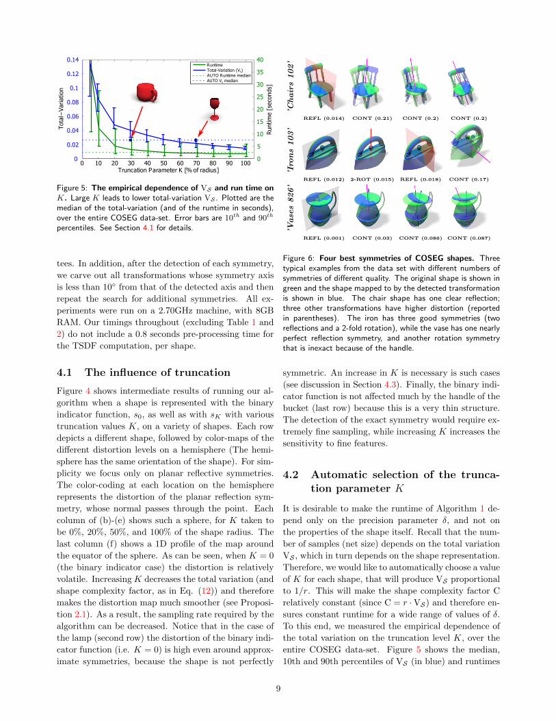
Figure 5: The empirical dependence of VS and run time onK. Large K leads to lower total-variation VS . Plotted are themedian of the total-variation (and of the runtime in seconds),over the entire COSEG data-set. Error bars are 10th and 90th

percentiles. See Section 4.1 for details.

tees. In addition, after the detection of each symmetry,

we carve out all transformations whose symmetry axis

is less than 10◦ from that of the detected axis and then

repeat the search for additional symmetries. All ex-

periments were run on a 2.70GHz machine, with 8GB

RAM. Our timings throughout (excluding Table 1 and

2) do not include a 0.8 seconds pre-processing time for

the TSDF computation, per shape.

4.1 The influence of truncation

Figure 4 shows intermediate results of running our al-

gorithm when a shape is represented with the binary

indicator function, s0, as well as with sK with various

truncation values K, on a variety of shapes. Each row

depicts a different shape, followed by color-maps of the

different distortion levels on a hemisphere (The hemi-

sphere has the same orientation of the shape). For sim-

plicity we focus only on planar reflective symmetries.

The color-coding at each location on the hemisphere

represents the distortion of the planar reflection sym-

metry, whose normal passes through the point. Each

column of (b)-(e) shows such a sphere, for K taken to

be 0%, 20%, 50%, and 100% of the shape radius. The

last column (f) shows a 1D profile of the map around

the equator of the sphere. As can be seen, when K = 0

(the binary indicator case) the distortion is relatively

volatile. Increasing K decreases the total variation (and

shape complexity factor, as in Eq. (12)) and therefore

makes the distortion map much smoother (see Proposi-

tion 2.1). As a result, the sampling rate required by the

algorithm can be decreased. Notice that in the case of

the lamp (second row) the distortion of the binary indi-

cator function (i.e. K = 0) is high even around approx-

imate symmetries, because the shape is not perfectly

’Chairs102’

REFL (0.014) CONT (0.21) CONT (0.2) CONT (0.2)

’Iro

ns103’

REFL (0.012) 2-ROT (0.015) REFL (0.018) CONT (0.17)

’Vase

s826’

REFL (0.001) CONT (0.03) CONT (0.086) CONT (0.087)

Figure 6: Four best symmetries of COSEG shapes. Threetypical examples from the data set with different numbers ofsymmetries of different quality. The original shape is shown ingreen and the shape mapped to by the detected transformationis shown in blue. The chair shape has one clear reflection;three other transformations have higher distortion (reportedin parentheses). The iron has three good symmetries (tworeflections and a 2-fold rotation), while the vase has one nearlyperfect reflection symmetry, and another rotation symmetrythat is inexact because of the handle.

symmetric. An increase in K is necessary is such cases

(see discussion in Section 4.3). Finally, the binary indi-

cator function is not affected much by the handle of the

bucket (last row) because this is a very thin structure.

The detection of the exact symmetry would require ex-

tremely fine sampling, while increasing K increases the

sensitivity to fine features.

4.2 Automatic selection of the trunca-

tion parameter K

It is desirable to make the runtime of Algorithm 1 de-

pend only on the precision parameter δ, and not on

the properties of the shape itself. Recall that the num-

ber of samples (net size) depends on the total variation

VS , which in turn depends on the shape representation.

Therefore, we would like to automatically choose a value

of K for each shape, that will produce VS proportional

to 1/r. This will make the shape complexity factor C

relatively constant (since C = r ·VS) and therefore en-

sures constant runtime for a wide range of values of δ.

To this end, we measured the empirical dependence of

the total variation on the truncation level K, over the

entire COSEG data-set. Figure 5 shows the median,

10th and 90th percentiles of VS (in blue) and runtimes

9

0 0.05 0.1 0.15 0.2 0.25Distortion

Groundtruth symmetriesGroundtruth asymmetries

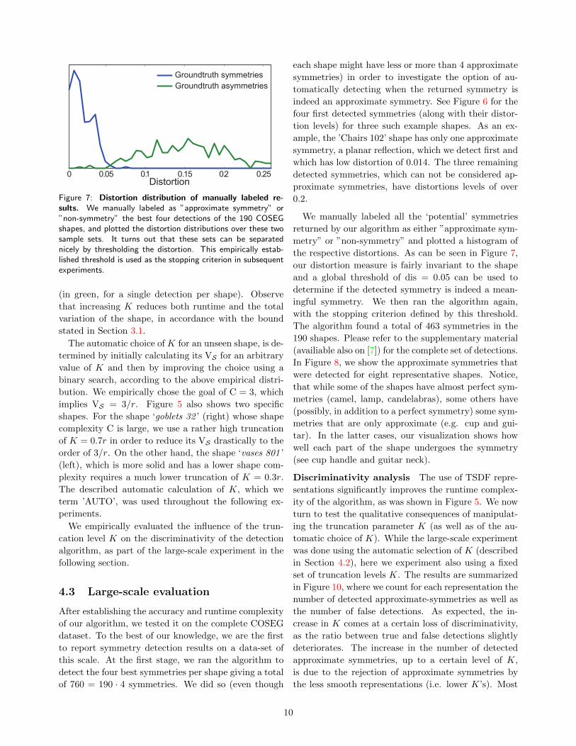
Figure 7: Distortion distribution of manually labeled re-sults. We manually labeled as ”approximate symmetry” or”non-symmetry” the best four detections of the 190 COSEGshapes, and plotted the distortion distributions over these twosample sets. It turns out that these sets can be separatednicely by thresholding the distortion. This empirically estab-lished threshold is used as the stopping criterion in subsequentexperiments.

(in green, for a single detection per shape). Observe

that increasing K reduces both runtime and the total

variation of the shape, in accordance with the bound

stated in Section 3.1.

The automatic choice of K for an unseen shape, is de-

termined by initially calculating its VS for an arbitrary

value of K and then by improving the choice using a

binary search, according to the above empirical distri-

bution. We empirically chose the goal of C = 3, which

implies VS = 3/r. Figure 5 also shows two specific

shapes. For the shape ‘goblets 32 ’ (right) whose shape

complexity C is large, we use a rather high truncation

of K = 0.7r in order to reduce its VS drastically to the

order of 3/r. On the other hand, the shape ‘vases 801 ’

(left), which is more solid and has a lower shape com-

plexity requires a much lower truncation of K = 0.3r.

The described automatic calculation of K, which we

term ’AUTO’, was used throughout the following ex-

periments.

We empirically evaluated the influence of the trun-

cation level K on the discriminativity of the detection

algorithm, as part of the large-scale experiment in the

following section.

4.3 Large-scale evaluation

After establishing the accuracy and runtime complexity

of our algorithm, we tested it on the complete COSEG

dataset. To the best of our knowledge, we are the first

to report symmetry detection results on a data-set of

this scale. At the first stage, we ran the algorithm to

detect the four best symmetries per shape giving a total

of 760 = 190 · 4 symmetries. We did so (even though

each shape might have less or more than 4 approximate

symmetries) in order to investigate the option of au-

tomatically detecting when the returned symmetry is

indeed an approximate symmetry. See Figure 6 for the

four first detected symmetries (along with their distor-

tion levels) for three such example shapes. As an ex-

ample, the ’Chairs 102’ shape has only one approximate

symmetry, a planar reflection, which we detect first and

which has low distortion of 0.014. The three remaining

detected symmetries, which can not be considered ap-

proximate symmetries, have distortions levels of over

0.2.

We manually labeled all the ‘potential’ symmetries

returned by our algorithm as either ”approximate sym-

metry” or ”non-symmetry” and plotted a histogram of

the respective distortions. As can be seen in Figure 7,

our distortion measure is fairly invariant to the shape

and a global threshold of dis = 0.05 can be used to

determine if the detected symmetry is indeed a mean-

ingful symmetry. We then ran the algorithm again,

with the stopping criterion defined by this threshold.

The algorithm found a total of 463 symmetries in the

190 shapes. Please refer to the supplementary material

(availiable also on [7]) for the complete set of detections.

In Figure 8, we show the approximate symmetries that

were detected for eight representative shapes. Notice,

that while some of the shapes have almost perfect sym-

metries (camel, lamp, candelabras), some others have

(possibly, in addition to a perfect symmetry) some sym-

metries that are only approximate (e.g. cup and gui-

tar). In the latter cases, our visualization shows how

well each part of the shape undergoes the symmetry

(see cup handle and guitar neck).

Discriminativity analysis The use of TSDF repre-

sentations significantly improves the runtime complex-

ity of the algorithm, as was shown in Figure 5. We now

turn to test the qualitative consequences of manipulat-

ing the truncation parameter K (as well as of the au-

tomatic choice of K). While the large-scale experiment

was done using the automatic selection of K (described

in Section 4.2), here we experiment also using a fixed

set of truncation levels K. The results are summarized

in Figure 10, where we count for each representation the

number of detected approximate-symmetries as well as

the number of false detections. As expected, the in-

crease in K comes at a certain loss of discriminativity,

as the ratio between true and false detections slightly

deteriorates. The increase in the number of detected

approximate symmetries, up to a certain level of K,

is due to the rejection of approximate symmetries by

the less smooth representations (i.e. lower K’s). Most

10

Candelab. 27 Candelab. 27 Candelab. 27 Candelab. 28 ’

REFL (0.004) REFL (0.010) 2-ROT (0.012) CONT (0.011)

Fourleg 393 Goblets 12 Guitars 427 Guitars 427

REFL (0.008) CONT (0.010) REFL (0.011) REFL (0.024)

Guitars 427 Lamps 18 ’ Vases 817 ’ Vases 817 ’

2-ROT (0.028) REFL (0.008) REFL (0.007) CONT (0.023)

Figure 8: Detected approximate symmetries on represen-tative COSEG shapes. Several examples - 8 shapes and the12 symmetries we detected for them, using the threshold fromFigure 7 as the largest admissible distortion. See the supple-mentary material for all 463 symmetries detected on the entiredataset.

noticeably, our automatic selection mode outperforms

any fixed selection of K in terms of the number of true

detections and the ratio of false detections as well as in

terms of runtime (see Figure 5).

4.4 Comparison with Kazhdan et al.[6]

As mentioned in Section 1.1, the work of Kazhdan et al

[6] bares some resemblance to the present work, mainly

because it also directly evaluates many transformations

using the measure of [20] and therefore some of our

bounds may apply to it. In spite of the similarities,

there are some major differences which make the com-

parison difficult. The methods mainly differ in the

choice of the set of transformations, as well as in the

1 2 3 4 5 6

Runtime (sec)

Figure 9: Distribution of runtime per detected symmetry,on the 463 detected symmetries in the COSEG data-set.

way by which they are evaluated.

The FFT-like approach in [6] requires a regular n×ngrid sampling of the latitude-longitude space of trans-

formations, where n is preferably a complete power of 2.

For this setting, the complexity of [6] is O(n4) , which is

dominated by an auto-correlation computation of order

O(n4), followed by a computation of order O(kn2) for

detecting k-fold symmetries for each k. In comparison,

our method’s complexity, O(n3 · ε−2 log 1p ), scales more

gracefully with n.

We first evaluated both methods on the task of de-

tecting the best symmetry in O(3) (including reflections

and rotations of up to 8 folds) for the shapes in the

COSEG data-set and compared several grid-size con-

figurations of [6] against our method. The publicly

available implementation of [6] does not allow access

to the O(n4) auto-correlation result and requires to re-

calculate it for each k-fold detection and therefore, for

fairness of comparison, we report the average time over

all k-fold computations for [6]. The results summarized

in Table 1 show that our method reaches lower distor-

tion values even when compared to a grid of 2562, which

takes much longer to evaluate. Note that all distortion

results are calculated on the original shape representa-

tion, following [20].

algorithmgridsize

numberoftrans.

distortion[20]

runtime[sec]

Kazhdanet al.[6]

322 1, 024 0.160 0.17642 4, 096 0.087 0.42

1282 16, 384 0.056 3.422562 65, 536 0.044 30.56

Proposedmethod

− 106, 054 0.040 2.62

Table 1: Best symmetry detection. The table summarizesperformance of two algorithms for best symmetry detection onthe COSEG data-set. Presented are median values for: (i)number of evaluated transformations (ii) symmetry measure[20] and (iii) run-time.

The sets of transformations used by both methods

are quite similar when limited to reflection symmetries,

therefore we were able to perform a more delicate com-

parison in this setting. We made several modifications

to our method so it would be directly comparable to

[6]. First, we set our net sizes to be equivalent to

the grid sizes in the code of [6], rather than follow-

ing Proposition 2.2 by using VS and δ. For the same

reason, we disabled the branch-and-bound procedure,

which allows reaching fine resolutions even with an ini-

tial coarse net. These modifications have a negative

impact on our algorithm. Note however that this com-

11

5 10 20 30 40 50 60 70 80 90 100 AUTO0

100

200

300

400

500

600

TruncationsparametersKs[bofsradius]

approximatessymmetries

falsesdetections

Tot

alsn

umbe

rsof

sdet

ectio

ns

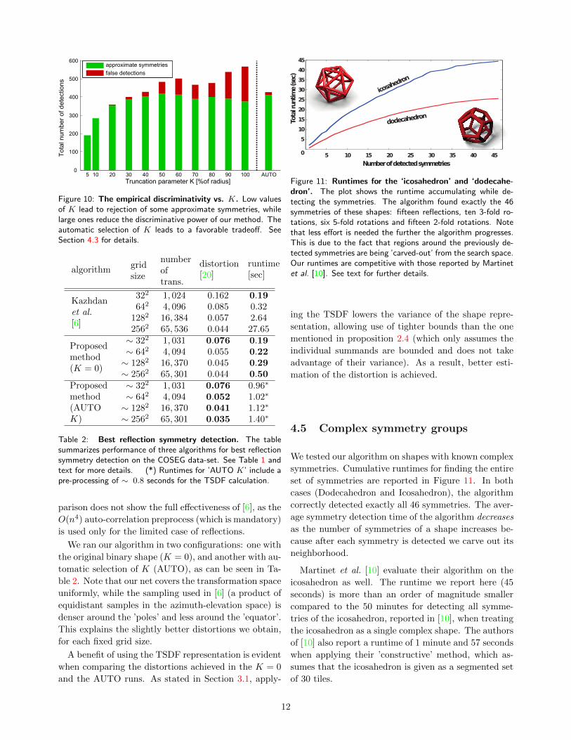
Figure 10: The empirical discriminativity vs. K. Low valuesof K lead to rejection of some approximate symmetries, whilelarge ones reduce the discriminative power of our method. Theautomatic selection of K leads to a favorable tradeoff. SeeSection 4.3 for details.

algorithmgridsize

numberoftrans.

distortion[20]

runtime[sec]

Kazhdanet al.[6]

322 1, 024 0.162 0.19642 4, 096 0.085 0.32

1282 16, 384 0.057 2.642562 65, 536 0.044 27.65

Proposedmethod(K = 0)

∼ 322 1, 031 0.076 0.19∼ 642 4, 094 0.055 0.22∼ 1282 16, 370 0.045 0.29∼ 2562 65, 301 0.044 0.50

Proposedmethod(AUTOK)

∼ 322 1, 031 0.076 0.96∗

∼ 642 4, 094 0.052 1.02∗

∼ 1282 16, 370 0.041 1.12∗

∼ 2562 65, 301 0.035 1.40∗

Table 2: Best reflection symmetry detection. The tablesummarizes performance of three algorithms for best reflectionsymmetry detection on the COSEG data-set. See Table 1 andtext for more details. (*) Runtimes for ’AUTO K’ include apre-processing of ∼ 0.8 seconds for the TSDF calculation.

parison does not show the full effectiveness of [6], as the

O(n4) auto-correlation preprocess (which is mandatory)

is used only for the limited case of reflections.

We ran our algorithm in two configurations: one with

the original binary shape (K = 0), and another with au-

tomatic selection of K (AUTO), as can be seen in Ta-

ble 2. Note that our net covers the transformation space

uniformly, while the sampling used in [6] (a product of

equidistant samples in the azimuth-elevation space) is

denser around the ’poles’ and less around the ’equator’.

This explains the slightly better distortions we obtain,

for each fixed grid size.

A benefit of using the TSDF representation is evident

when comparing the distortions achieved in the K = 0

and the AUTO runs. As stated in Section 3.1, apply-

5 10 15 20 25 30 35 40 450

5

10

15

20

25

30

35

40

45

Numberofdetectedsymmetries

Totalruntim

e(sec)

dodecahedron

icosahe

dron

Figure 11: Runtimes for the ‘icosahedron’ and ‘dodecahe-dron’. The plot shows the runtime accumulating while de-tecting the symmetries. The algorithm found exactly the 46symmetries of these shapes: fifteen reflections, ten 3-fold ro-tations, six 5-fold rotations and fifteen 2-fold rotations. Notethat less effort is needed the further the algorithm progresses.This is due to the fact that regions around the previously de-tected symmetries are being ’carved-out’ from the search space.Our runtimes are competitive with those reported by Martinetet al. [10]. See text for further details.

ing the TSDF lowers the variance of the shape repre-

sentation, allowing use of tighter bounds than the one

mentioned in proposition 2.4 (which only assumes the

individual summands are bounded and does not take

advantage of their variance). As a result, better esti-

mation of the distortion is achieved.

4.5 Complex symmetry groups

We tested our algorithm on shapes with known complex

symmetries. Cumulative runtimes for finding the entire

set of symmetries are reported in Figure 11. In both

cases (Dodecahedron and Icosahedron), the algorithm

correctly detected exactly all 46 symmetries. The aver-

age symmetry detection time of the algorithm decreases

as the number of symmetries of a shape increases be-

cause after each symmetry is detected we carve out its

neighborhood.

Martinet et al. [10] evaluate their algorithm on the

icosahedron as well. The runtime we report here (45

seconds) is more than an order of magnitude smaller

compared to the 50 minutes for detecting all symme-

tries of the icosahedron, reported in [10], when treating

the icosahedron as a single complex shape. The authors

of [10] also report a runtime of 1 minute and 57 seconds

when applying their ’constructive’ method, which as-

sumes that the icosahedron is given as a segmented set

of 30 tiles.

12

REFL (0.0068) REFL (0.0282) REFL (0.0496) 2-ROT (0.1004) CONT (0.1686)

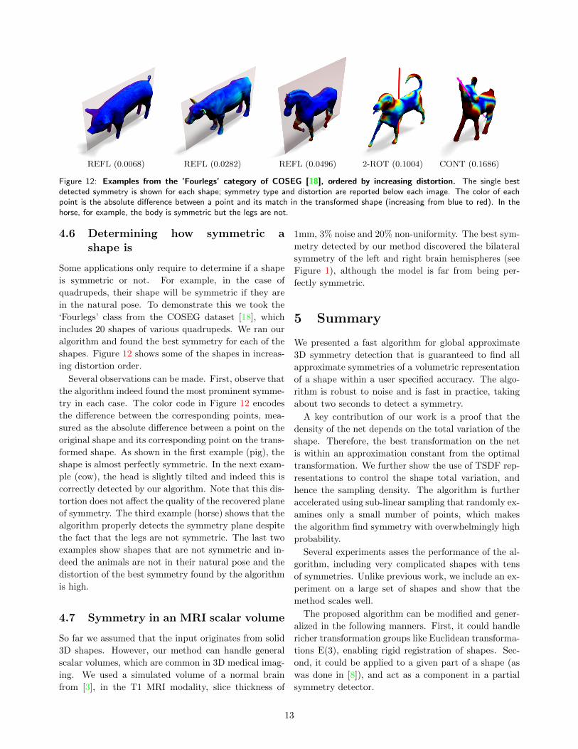
Figure 12: Examples from the ’Fourlegs’ category of COSEG [18], ordered by increasing distortion. The single bestdetected symmetry is shown for each shape; symmetry type and distortion are reported below each image. The color of eachpoint is the absolute difference between a point and its match in the transformed shape (increasing from blue to red). In thehorse, for example, the body is symmetric but the legs are not.

4.6 Determining how symmetric a

shape is

Some applications only require to determine if a shape

is symmetric or not. For example, in the case of

quadrupeds, their shape will be symmetric if they are

in the natural pose. To demonstrate this we took the

‘Fourlegs’ class from the COSEG dataset [18], which

includes 20 shapes of various quadrupeds. We ran our

algorithm and found the best symmetry for each of the

shapes. Figure 12 shows some of the shapes in increas-

ing distortion order.

Several observations can be made. First, observe that

the algorithm indeed found the most prominent symme-

try in each case. The color code in Figure 12 encodes

the difference between the corresponding points, mea-

sured as the absolute difference between a point on the

original shape and its corresponding point on the trans-

formed shape. As shown in the first example (pig), the

shape is almost perfectly symmetric. In the next exam-

ple (cow), the head is slightly tilted and indeed this is

correctly detected by our algorithm. Note that this dis-

tortion does not affect the quality of the recovered plane

of symmetry. The third example (horse) shows that the

algorithm properly detects the symmetry plane despite

the fact that the legs are not symmetric. The last two

examples show shapes that are not symmetric and in-

deed the animals are not in their natural pose and the

distortion of the best symmetry found by the algorithm

is high.

4.7 Symmetry in an MRI scalar volume

So far we assumed that the input originates from solid

3D shapes. However, our method can handle general

scalar volumes, which are common in 3D medical imag-

ing. We used a simulated volume of a normal brain

from [3], in the T1 MRI modality, slice thickness of

1mm, 3% noise and 20% non-uniformity. The best sym-

metry detected by our method discovered the bilateral

symmetry of the left and right brain hemispheres (see

Figure 1), although the model is far from being per-

fectly symmetric.

5 Summary

We presented a fast algorithm for global approximate

3D symmetry detection that is guaranteed to find all

approximate symmetries of a volumetric representation

of a shape within a user specified accuracy. The algo-

rithm is robust to noise and is fast in practice, taking

about two seconds to detect a symmetry.

A key contribution of our work is a proof that the

density of the net depends on the total variation of the

shape. Therefore, the best transformation on the net

is within an approximation constant from the optimal

transformation. We further show the use of TSDF rep-

resentations to control the shape total variation, and

hence the sampling density. The algorithm is further

accelerated using sub-linear sampling that randomly ex-

amines only a small number of points, which makes

the algorithm find symmetry with overwhelmingly high

probability.

Several experiments asses the performance of the al-

gorithm, including very complicated shapes with tens

of symmetries. Unlike previous work, we include an ex-

periment on a large set of shapes and show that the

method scales well.

The proposed algorithm can be modified and gener-

alized in the following manners. First, it could handle

richer transformation groups like Euclidean transforma-

tions E(3), enabling rigid registration of shapes. Sec-

ond, it could be applied to a given part of a shape (as

was done in [8]), and act as a component in a partial

symmetry detector.

13

References

[1] Dror Aiger, Niloy J Mitra, and Daniel Cohen-Or.

4-points congruent sets for robust pairwise surface

registration. In ACM Transactions on Graphics

(TOG), volume 27, page 85. ACM, 2008.

[2] Mikhail J. Atallah. On symmetry detection. Com-

puters, IEEE Transactions on, C-34(7):663–666,

1985.

[3] Chris A. Cocosco, Vasken Kollokian, Remi K.-S.

Kwan, G. Bruce Pike, and Alan C. Evans. Brain-

web: Online interface to a 3d mri simulated brain

database. NeuroImage, 5:425, 1997.

[4] Yuval Eldar, Michael Lindenbaum, Moshe Porat,

and Yehoshua Y Zeevi. The farthest point strategy

for progressive image sampling. Trans. on Imag.

Proc., 6(9):1305–1315, 1997.

[5] Hagit Hel-Or and Craig S Kaplan. Computational

symmetry in computer vision and computer graph-

ics. Now publishers Inc, 2010.

[6] Michael Kazhdan, Thomas Funkhouser, and Szy-

mon Rusinkiewicz. Symmetry descriptors and 3d

shape matching. In SGP, pages 115–123. ACM,

2004.

[7] Simon Korman, Roee Litman, Shai Avidan, and

Alex Bronstein. Probably approximately sym-

metric webpage. www.eng.tau.ac.il/~simonk/

ShapeSymmetry/index.html.

[8] Simon Korman, Daniel Reichman, Gilad Tsur, and

Shai Avidan. Fast-match: Fast affine template

matching. In CVPR, pages 2331–2338. IEEE, 2013.

[9] Yaron Lipman, Xiaobai Chen, Ingrid Daubechies,

and Thomas A. Funkhouser. Symmetry factored

embedding and distance. ACM Trans. Graph.,

29(4), 2010.

[10] A. Martinet, C. Soler, N. Holzschuch, and F. Sil-

lion. Accurate detection of symmetries in 3d

shapes. ACM Transactions on Graphics (TOG),

25(2):439–464, 2006.

[11] Niloy J. Mitra, Leonidas J. Guibas, and Mark

Pauly. Partial and approximate symmetry de-

tection for 3d geometry. ACM Trans. Graph.,

25(3):560–568, 2006.

[12] Niloy J. Mitra, Mark Pauly, Michael Wand, and

Duygu Ceylan. Symmetry in 3d geometry: Ex-

traction and applications. In EUROGRAPHICS

State-of-the-art Report, 2012.

[13] Maks Ovsjanikov, Jian Sun, and Leonidas Guibas.

Global intrinsic symmetries of shapes. In Proceed-

ings of the Symposium on Geometry Processing,

SGP ’08, pages 1341–1348, 2008.

[14] J. Podolak, P. Shilane, A. Golovinskiy,

S. Rusinkiewicz, and T. Funkhouser. A planar-

reflective symmetry transform for 3d shapes.

In ACM Transactions on Graphics (TOG),

volume 25, pages 549–559. ACM, 2006.

[15] Raviv, A. M. Bronstein, M. M. Bronstein, and

R. Kimmel. Full and partial symmetries of non-

rigid shapes. Intl. Journal of Computer Vision

(IJCV), 89(1):189–39, 2010.

[16] Changming Sun and Jamie Sherrah. 3d symmetry

detection using the extended gaussian image. IEEE

Trans. Pattern Anal. Mach. Intell., 19(2):164–168,

1997.

[17] Leslie G Valiant. A theory of the learnable. Com-

munications of the ACM, 27(11):1134–1142, 1984.

[18] Yunhai Wang, Shmulik Asafi, Oliver van Kaick,

Hao Zhang, Daniel Cohen-Or, and Baoquan Chen.

Active co-analysis of a set of shapes. ACM Trans-

actions on Graphics (TOG), 31(6), 2012.

[19] JanD. Wolter, TonyC. Woo, and RichardA. Volz.

Optimal algorithms for symmetry detection in two

and three dimensions. The Visual Computer,

1(1):37–48, 1985.

[20] Hagit Zabrodsky, Shmuel Peleg, and David Avnir.

Symmetry as a continuous feature. Pattern Anal-

ysis and Machine Intelligence, IEEE Transactions

on, 17(12):1154–1166, 1995.

14