probability: sequence overview - resolve | … · probability: sequence overview ... the sequence...
TRANSCRIPT
PROBABILITY: Sequence Overview Summary of learning goals The sequence begins by reviewing earlier ideas of probability and everyday situations where probability is relevant. Students calculate probabilities in a variety of situations where outcomes are equally likely, as fractions, decimals and percentages. They learn about the variability of the outcomes in an experiment with a small sample size, and the stability of the outcomes for a large number of trials; an instance of the law of large numbers which is the basis of statistics. They use this important knowledge in two situations where they sample to make predictions about the populations.
Australian Curriculum: Mathematics (Year 6)
ACMSP144: Describe probabilities using fractions, decimals and percentages. ACMSP145: Conduct chance experiments with both small and large numbers of trials using appropriate digital technologies. ACMSP146: Compare observed frequencies across experiments with expected frequencies.
Summary of lessons Who is this Sequence for?
This sequence is designed for students who have already encountered probability in simple situations, and know that a probability is a fraction between 0 and 1 that indicates the chance of an event occurring. Students need some familiarity with converting between fractions, decimals and percentages, and in finding a percentage of a number, and the sequence provides further practice for these skills. Lessons 3 and 4 are also suitable for older students to review the probability basis of making predictions from surveys.
Lesson 1: Four-tunate Fours
This lesson explores probability in some real world settings. Students examine (fictitious) magazine covers that show statements of chance in sport and money settings in everyday language and link to probability language. They represent probabilities as fractions, decimals and percentages. They discuss probabilities that arise in playing a game of chance, and use this information when creating their own unfair game of chance.
Lesson 2: 30 300 3000
After a brief introduction about ‘lucky’ and ‘unlucky’ numbers, students collect data by rolling dice themselves and later use a spreadsheet to simulate rolling dice from 30 to 300 to 3000 times. They see the effect that changing sample size has on the frequency of each outcome, and on percent frequency, and they calculate simple measures of the variation in the outcomes. They draw column graphs to show these differences.
Lesson 3: Alice
The task is to predict the number of times selected letters occur in the first 5000 letters from “Alice in Wonderland”. Students take samples from which to predict the number of times selected letters occur. From observed frequencies in the sample, they calculate relative frequencies as fractions, decimals and percent. They use the percent frequency to make the prediction of real frequency in all 5000 letters. They stop when they think the sample is large enough for the prediction to be reliable, and then compare with the actual distribution.
2
Lesson 4: Plenty More Fish in the Sea
Students gather data about a population by sampling. They start in a whole class introduction with a small set of unseen counters in a bag and work out the proportion of colours in the bag by sampling and replacing. ‘Tagged fish’ are introduced into the bag so that the numbers of counters in the bag can be estimated. This method is then applied to estimate the population of the school playground by releasing students as ‘tagged fish’ at break time.
Reflection on this Sequence
Rationale
This series of lessons is carefully sequenced to lead the students to a deeper understanding of the applications for probability. The sequence starts by looking at the expectations of certain outcomes of chance events occurring, expressing simple probabilities as fractions, decimals or percentages including in games. In the second lesson, students explore the idea of “short-run variability and long-run stability”. The students will quickly observe wide variation in their results when they conduct small-scale trials or sample a small set of data. They then see that the variation in percentage frequency reduces as the number of trials increases and their results conform to expected theoretical probabilities. This gives students practical experience of how variation in the results reduces as the number of trials in a chance experiment increases. In the final two lessons, the sequence concludes by turning this situation around. This time we have an unknown theoretical probability, and the students’ job is to find it. We gather information through a survey, calculate a probability from the sample, and use it to estimate the actual probability of these events.
“Chance and data” are often taught as two very separate topics. Much can be gained, however, by considering them together. This is especially the situation in surveys and opinion polls, which are used find out information about a whole population in the common situation when there is no capacity to ask everybody. If you use a random sample which is large enough, you can get a good estimate of the probabilities involved. An important thing is that to make a good prediction not everyone needs to be asked.
reSolve Mathematics is Purposeful
Problem solving encourages students to ask questions and then find solutions using their knowledge of probability. A wide range of real world situations are included in the sequence, from simple instances of interpreting common language about everyday events to estimating the distribution of letters in an English text and conducting a capture-mark-recapture experiment as is used by ecologists to estimate wild animal populations. This sequence of lessons also provides an opportunity for students to develop an understanding of the relationship between fractions, decimals and percentages, as well as understanding the nature of probability in making good predictions.
reSolve Tasks are Challenging Yet Accessible
The lessons presented here start with easily accessible games that provide a common experience and observations that students will be able to quickly understand in real world terms. Students with different home backgrounds will be able to contribute different understandings.
reSolve Classrooms Have a Knowledge Building Culture
Games and activities that involve chance are fun and enjoyable and provide students with opportunities to work together. Through interaction with others and by allowing students to discuss their experiences, a community of learners can be established and reinforced within the classroom.
We value your feedback after these lessons via http://tiny.cc/lesson-feedback
We value your feedback after this lesson via http://tiny.cc/lesson-feedback
PROBABILITY Lesson 1: Four-tunate Fours Australian Curriculum: Mathematics – Year 6 ACMSP144: Describe probabilities using fractions, decimals and percentages. ACMSP145: Conduct chance experiments with both small and large numbers of trials using appropriate digital technologies.
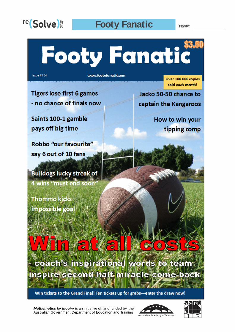
Lesson abstract This lesson explores probability in some real world settings. Students examine (fictitious) magazine covers that show statements of chance in sport and money settings in everyday language and link to probability language. They represent probabilities as fractions, decimals and percentages. They discuss probabilities that arise in playing a game of chance, and use this information when creating their own unfair game of chance.
Mathematical purpose (for students) Probabilities can be described using fractions, decimals and percentages.
Mathematical purpose (for teachers) This lesson builds a bridge to probability language through common situations and language. Students review their prior understanding of probability as the fraction of all outcomes that are favourable and apply this by counting outcomes for choosing numbers from a hundreds chart, and by finding some simple probabilities related to games. They consider whether the probabilities of winning are equal for all players in an interesting game, discuss fairness in probability terms and design a game where the probabilities of winning are not equal.
At the end of this lesson, students will be able to:
• Describe the probability of an event using fractions, decimals and percentages. • Define key language for use with probability activities. • Explain how a game can be unfair and biased in favour of one player.
Lesson Length 90 minutes approximately
Vocabulary Encountered • chance • probability • random • fair • biased • equally likely
Lesson Materials • large class 100s chart • dice – at least 2 per student (more is good) • Student Sheet 1 – Footy Fanatic (1 per 2 students) • Student Sheet 2 – Know More Money (1 per 2 students • Student Sheet 3 - Expressing Probabilities (1 per student) • Student Sheet 4 - Statements of Chance (1 per student) • Board games such as Ludo, Sorry etc.
2
Probability in Everyday Life
Provocation – statements of probability in advertising • Divide the class into pairs. Give to each pair the two fictitious magazine covers in Student Sheet 1 – Footy
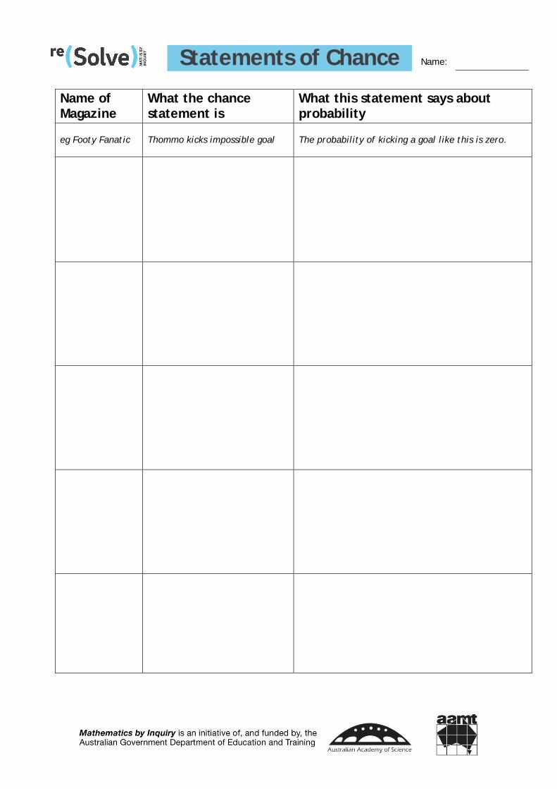
Fanatic and Student Sheet 2 – Know More Money. • Draw attention to some of the statements involving chance and uncertainty. • Ask students to complete the table in Student Sheet 4 - Statements of Chance to show:
o Name of magazine. o What the statement about chance (probability) is. o What this statement says about probability more precisely.
• Discuss student responses to each of the magazine cover statements.
Teacher Notes
• It would be good for students to have colour copies of the magazine covers to look at. • There are many interesting issues relating to probability that are represented in these (fictional)
advertisements. • This introduction is to link everyday words like chance, odds and luck to probability, to observe how
probability statements are expressed in common language, and how probability concepts are relevant in many walks of life.
• See Ideas about Chance from the Magazine Covers for more discussion of the ideas.
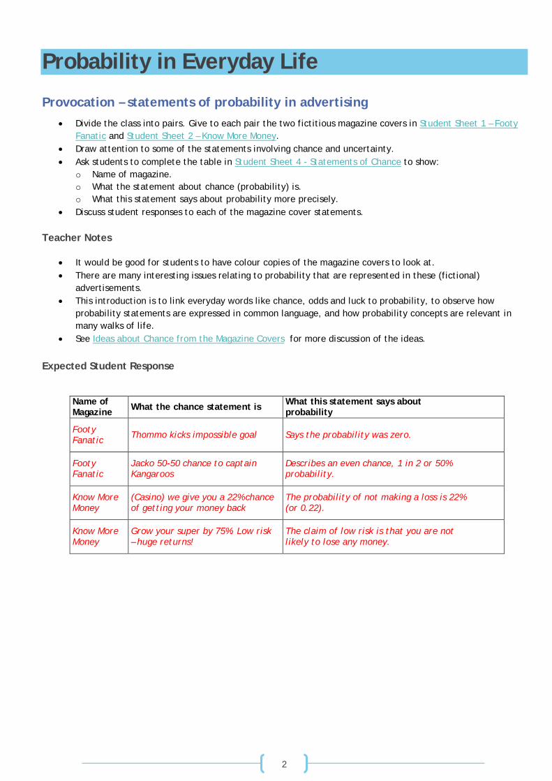
Expected Student Response
Name of Magazine What the chance statement is What this statement says about
probability
Footy Fanatic Thommo kicks impossible goal Says the probability was zero.
Footy Fanatic
Jacko 50-50 chance to captain Kangaroos
Describes an even chance, 1 in 2 or 50% probability.
Know More Money
(Casino) we give you a 22% chance of getting your money back
The probability of not making a loss is 22% (or 0.22).
Know More Money
Grow your super by 75%. Low risk – huge returns!
The claim of low risk is that you are not likely to lose any money.
3
Describing Probabilities
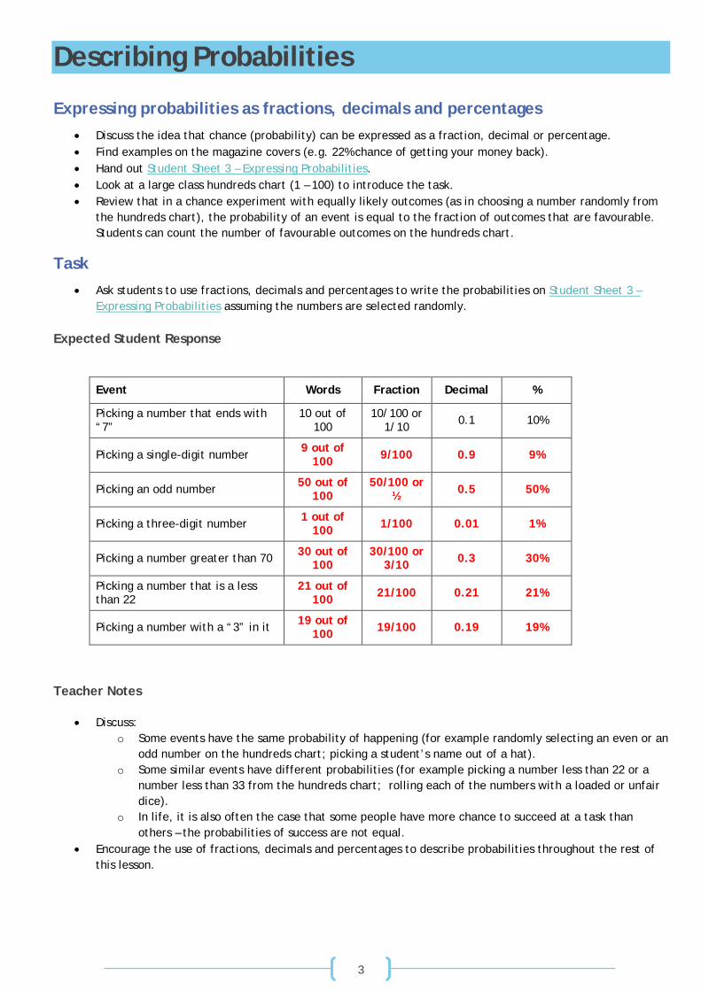
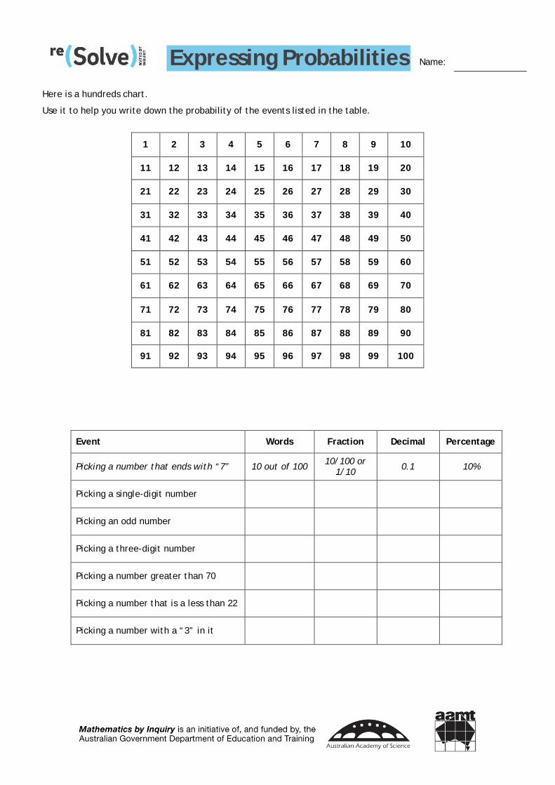
Expressing probabilities as fractions, decimals and percentages • Discuss the idea that chance (probability) can be expressed as a fraction, decimal or percentage. • Find examples on the magazine covers (e.g. 22% chance of getting your money back). • Hand out Student Sheet 3 – Expressing Probabilities. • Look at a large class hundreds chart (1 – 100) to introduce the task. • Review that in a chance experiment with equally likely outcomes (as in choosing a number randomly from
the hundreds chart), the probability of an event is equal to the fraction of outcomes that are favourable. Students can count the number of favourable outcomes on the hundreds chart.
Task • Ask students to use fractions, decimals and percentages to write the probabilities on Student Sheet 3 –
Expressing Probabilities assuming the numbers are selected randomly. Expected Student Response
Teacher Notes
• Discuss: o Some events have the same probability of happening (for example randomly selecting an even or an
odd number on the hundreds chart; picking a student’s name out of a hat). o Some similar events have different probabilities (for example picking a number less than 22 or a
number less than 33 from the hundreds chart; rolling each of the numbers with a loaded or unfair dice).
o In life, it is also often the case that some people have more chance to succeed at a task than others – the probabilities of success are not equal.
• Encourage the use of fractions, decimals and percentages to describe probabilities throughout the rest of this lesson.
Event Words Fraction Decimal %
Picking a number that ends with “7”
10 out of 100
10/100 or 1/10 0.1 10%
Picking a single-digit number 9 out of 100 9/100 0.9 9%
Picking an odd number 50 out of 100
50/100 or ½ 0.5 50%
Picking a three-digit number 1 out of 100 1/100 0.01 1%
Picking a number greater than 70 30 out of 100
30/100 or 3/10 0.3 30%
Picking a number that is a less than 22
21 out of 100 21/100 0.21 21%
Picking a number with a “3” in it 19 out of 100 19/100 0.19 19%
4
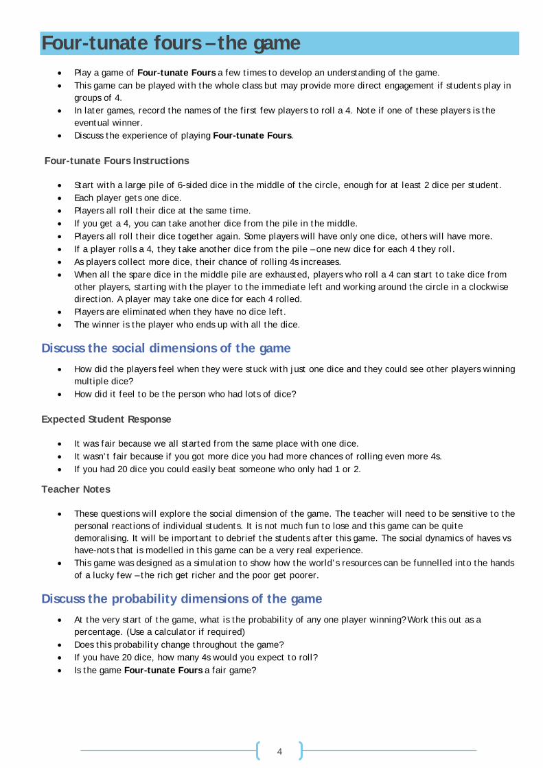
Four-tunate fours – the game
• Play a game of Four-tunate Fours a few times to develop an understanding of the game. • This game can be played with the whole class but may provide more direct engagement if students play in
groups of 4. • In later games, record the names of the first few players to roll a 4. Note if one of these players is the
eventual winner. • Discuss the experience of playing Four-tunate Fours.
Four-tunate Fours Instructions
• Start with a large pile of 6-sided dice in the middle of the circle, enough for at least 2 dice per student. • Each player gets one dice. • Players all roll their dice at the same time. • If you get a 4, you can take another dice from the pile in the middle. • Players all roll their dice together again. Some players will have only one dice, others will have more. • If a player rolls a 4, they take another dice from the pile – one new dice for each 4 they roll. • As players collect more dice, their chance of rolling 4s increases. • When all the spare dice in the middle pile are exhausted, players who roll a 4 can start to take dice from
other players, starting with the player to the immediate left and working around the circle in a clockwise direction. A player may take one dice for each 4 rolled.
• Players are eliminated when they have no dice left. • The winner is the player who ends up with all the dice.
Discuss the social dimensions of the game • How did the players feel when they were stuck with just one dice and they could see other players winning
multiple dice? • How did it feel to be the person who had lots of dice?
Expected Student Response
• It was fair because we all started from the same place with one dice. • It wasn’t fair because if you got more dice you had more chances of rolling even more 4s. • If you had 20 dice you could easily beat someone who only had 1 or 2.
Teacher Notes
• These questions will explore the social dimension of the game. The teacher will need to be sensitive to the personal reactions of individual students. It is not much fun to lose and this game can be quite demoralising. It will be important to debrief the students after this game. The social dynamics of haves vs have-nots that is modelled in this game can be a very real experience.
• This game was designed as a simulation to show how the world’s resources can be funnelled into the hands of a lucky few – the rich get richer and the poor get poorer.
Discuss the probability dimensions of the game • At the very start of the game, what is the probability of any one player winning? Work this out as a
percentage. (Use a calculator if required) • Does this probability change throughout the game? • If you have 20 dice, how many 4s would you expect to roll? • Is the game Four-tunate Fours a fair game?
5
Expected Student Response
• The probability of a player winning at the start is the same for each player. As a % it will be (1 ÷ the number of players) x 100.
• During the game, the probability of winning will increase for some and decrease for others. It will depend on how many dice the player has, and also on how many dice are held by close neighbours who might take from them.
• I would expect 1/6 of them to be a 4. If I had 20 dice that would be 20 ÷ 6 = 3r2 so I would expect about three 4s.
• While all players have the same probability of winning at the start of the game, this quickly changes as the game has a strong bias towards players who roll 4 early in the game.
Using Language Appropriately
The language of probability • Review the ideas of “probability” and “random” – discuss what these words mean and how we use them. • Brainstorm other words that are used to describe probability and discuss their meanings and use.
Teacher Notes
• It is important to clarify the correct meaning of “random” as the selection of objects from a set where each object has an equal chance of being selected. “Random” has taken on a modern variation where it can mean odd or peculiar in an amusing kind of way, or also unknown or unfamiliar.
• Here are the etymological roots of some words related to probability:
o chance - from Old French cheance "accident, chance, fortune, luck, situation, the falling of dice, from Vulgar Latin cadentia "that which falls out," a term used in dice
o fair – Old English fægere, early 13th century as "according with propriety; according with justice," and mid-14th century "equitable, impartial, just, free from bias"
o frequency – from Latin frequentia meaning a crowd, multitude, throng o luck - from early Middle Dutch luc, shortening of gheluc "happiness, good fortune," of unknown
origin. It has cognates in Dutch geluk, Middle High German g(e)lücke, German Glück "fortune, good luck”
o possibility - from Latin possibilis "that can be done," from posse "be able" o probability – from Latin probabilis meaning provable or credible o random – from Old French randon to rush; disorder and impetuosity; Old High German rennen to
run o These words and others can be sourced at http://www.etymonline.com
Make Your Own Game
The unfair game • Discuss the idea of a fair and unfair game. In a fair game, all players have the same probability of winning
at the start. • Ask students to design their own unfair game, where one player has greater chance of winning (or losing)
than the other players. However, everyone must be able to win sometimes. • They may wish to modify the rules of a well-known game such as Snakes and Ladders or Ludo to make it
unfair.
6
Teacher Notes
• Observing what the students produce will provide good evidence of their learning. If they can show how the game is biased and use the language of probability to explain the bias, they will demonstrate the depth of their understanding of the concepts involved.
• Students will need to play the game to check that the rules work as expected. They will also need to explain carefully what makes it unfair and that it is still possible for all players to win.
Expected Student Response
• We played Snakes and Ladders with 2 dice. Player 1 had to add the dice rolls together. Player 2 got to multiply them. The furthest Player 1 could move was 12 squares but Player 2 could move 36 squares if they got a double 6.
• We played Scissors, Paper, Rock. If there was a draw, Player 1 was the winner. Player 1 had 6 out of 9 chances to win, twice as many chances as Player 2 had.
• We played Snakes and Ladders. Player 1 could only move when an odd number was rolled. Player 2 could only move if even numbers were rolled. This meant that both players could only move for an expected 50% of their dice rolls but for each roll Player 2 would get to move 1 square further on average than Player 1.
Additional Tasks
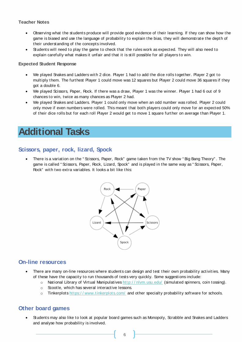
Scissors, paper, rock, lizard, Spock • There is a variation on the “Scissors, Paper, Rock” game taken from the TV show “Big Bang Theory”. The
game is called “Scissors, Paper, Rock, Lizard, Spock” and is played in the same way as “Scissors, Paper, Rock” with two extra variables. It looks a bit like this:
On-line resources • There are many on-line resources where students can design and test their own probability activities. Many
of these have the capacity to run thousands of tests very quickly. Some suggestions include: o National Library of Virtual Manipulatives http://nlvm.usu.edu/ (simulated spinners, coin tossing). o Scootle, which has several interactive lessons. o Tinkerplots https://www.tinkerplots.com/ and other specialty probability software for schools.
Other board games • Students may also like to look at popular board games such as Monopoly, Scrabble and Snakes and Ladders
and analyse how probability is involved.
7
Ideas about Chance from the Magazine Covers
“Footy Fanatic” discussion points
Tigers lose first 6 games – no chance of finals now • Even after such a poor start to the season, in most of the national football codes there are over 20 rounds
of games before the finals grouping is decided. So the Tigers should still have a chance (probability not zero) of making the finals.
• However, football success relies on player confidence and a team that loses regularly early on in the season has a low probability of turning this around very quickly.
• The early results show that at least 6 teams in the competition are better than the Tigers. Most finals play-off rounds involve 8 teams, so there are still 2 places left for the Tigers.
Saints 100-1 gamble pays off big time • A “gamble” indicates that there were some choices involved for the Saints and that these choices involved
a degree of uncertainty. • A 100-1 gamble is a long shot, very unlikely to occur. This means the probability of the action failing was
100 times more than the probability of success. Bulldogs lucky streak of 4 wins “must end soon”
• Describing the 4 wins as a “lucky streak” suggests that this result was unexpected (i.e. its estimated probability was low).
• Future results are not directly dependent on past results so there is the potential for the winning streak to continue for a long time – or to end next week.
Thommo kicks impossible goal
• If it was impossible, then Thommo could not have done it. Having kicked the goal, Thommo has proved that it wasn’t impossible.
Jacko 50-50 chance to captain the Kangaroos
• 50-50 means it is as likely that he will become the captain as that he won’t. • A 50% chance says the probability is one half (also 0.5 or 50%).
How to win your tipping comp
• A “tipping comp” involves people making predictions about the outcomes of future football games. There are many different systems that people use to make these predications. None of them are 100% successful. There is always an element of risk in making predictions about future outcomes.
Win tickets to the Grand Final! Ten tickets up for grabs – enter the draw now!
• “Up for grabs” means the tickets are available. • A “draw” means a lottery where the names of a winner will be selected at random. • If there is a circulation of 100 000 copies sold each month and only 10 tickets, your chances of winning are
less than 1 in 10 000.
8
“Know More Money” discussion points Grow your super by 75%. Low risk – huge returns!
• “Super” means superannuation, an arrangement where the government supports people to put money away during their working lives to live on when they retire.
• 75% return on a superannuation investment is very unlikely. High rates of return are typically associated with high risk, so not a wise choice for superannuation.
Improve your chances on the stock market by half!
• This might mean that the probability of making a profit on a stock is increased by 50%. Are casinos still a good bet? – we give you a 22% chance of getting your money back!
• Casinos survive because the probability is that they will win more money than they pay out at the games they offer. However, to entice people to play, they do offer some high returns for unlikely outcomes.
• 22% is a very low chance of getting your money back. Top investments for the year as picked by our astrologer
• Using astrology to make financial decisions is not a reliable strategy. Get rich quick – send us $1000 and we will give one lucky reader $1 million!
• A huge return for the investor that is prepared to put in $1000 but the chance of winning is uncertain. We don’t know how many other people will also be involved. There will need to be at least 1000 people for the magazine to come out ahead.
• Also, there are no details about how the lucky reader will be selected. Profit or loss – is it a 50-50 chance?
• This is an ‘experiment’ with two possible outcomes – profit or loss – but this does not mean that the probability of each is a half. The outcomes are not usually equally likely.
The #1 Investment magazine
• Having looked at the cover, a reader may be inclined to doubt this claim.
Footy Fanatic Name:
Student Sheet 1 - Footy Fan atic

Know More Money Name:
Student Sheet 2 – Know Mo re Money
Expressing Probabilities Name:
Student Sheet 3 – E xpre ssing P robabilit ies
Here is a hundreds chart.
Use it to help you write down the probability of the events listed in the table.
1 2 3 4 5 6 7 8 9 10
11 12 13 14 15 16 17 18 19 20
21 22 23 24 25 26 27 28 29 30
31 32 33 34 35 36 37 38 39 40
41 42 43 44 45 46 47 48 49 50
51 52 53 54 55 56 57 58 59 60
61 62 63 64 65 66 67 68 69 70
71 72 73 74 75 76 77 78 79 80
81 82 83 84 85 86 87 88 89 90
91 92 93 94 95 96 97 98 99 100
Event Words Fraction Decimal Percentage
Picking a number that ends with “7” 10 out of 100 10/100 or 1/10 0.1 10%
Picking a single-digit number
Picking an odd number
Picking a three-digit number
Picking a number greater than 70
Picking a number that is a less than 22
Picking a number with a “3” in it
Statements of Chance Name:
Student Sheet 4 – Statements of Ch ance
Name of Magazine
What the chance statement is
What this statement says about probability
eg Footy Fanatic Thommo kicks impossible goal The probability of kicking a goal like this is zero.
We value your feedback after this lesson via http://tiny.cc/lesson-feedback
PROBABILITY Lesson 2: 30 300 3000 Australian Curriculum: Mathematics – Year 6 ACMSP144: Describe probabilities using fractions, decimals and percentages. ACMSP145: Conduct chance experiments with both small and large numbers of trials using appropriate digital technologies. ACMSP146: Compare observed frequencies across experiments with expected frequencies.
Lesson abstract This lesson explores one of the most important aspects of probability. After a brief introduction about ‘lucky’ and ‘unlucky’ numbers, students collect data by rolling dice themselves and later use a spreadsheet to simulate rolling dice first 30, then 300, then 3000 times. They see the effect that changing sample size has on the frequency of each outcome, and on percent frequency, and they calculate simple measures of the variation in the outcomes. They draw column graphs to show these differences.
Mathematical purpose (for students) If you roll a dice many times, you can be confident that each number will occur about a sixth of the time. If you only roll it a few times, there is much more variation.
Mathematical purpose (for teachers) Students participate in data collection that demonstrates part of the ‘law of large numbers’ which is the basis of statistics. They see that the outcomes of a chance experiment with a small sample are unpredictable but outcomes from a large sample are close to the proportions predicted by probability. They calculate a simple measure of variation that shows the short-term variability but long-term stability in the percent frequency of outcomes. At the end of this lesson, students will be able to:
• Explain why it is important to know the size of a sample. • Describe what happens to data variability when you increase your sample size.
Lesson Length 90 minutes approximately
Vocabulary Encountered • sample size • outcome • frequency • prediction • variation
Lesson Materials • dice (one per student) • Slideshow – Increasing Sample Size 2a Probability 30 300 3000 powerpoint • Spreadsheet – 30 300 3000 2b Probability 30 300 3000 spreadsheet
• Student Sheet 1 – Individual Data (1 per student) • Student Sheet 2 – Class Data (1 per student) • Student Sheet 3 – Reflection 30 300 3000 (1 per student)
2
Introduction Slideshow – “Increasing sample size” The slide show: Increasing Sample Size 2a Probability 30 300 3000 powerpoint can be used to structure this lesson.
Slide 3 – lucky and unlucky numbers • Introduce class discussion about lucky and unlucky numbers around the world. • Some examples are on slide 2 (e.g. 8 is a lucky number in China because it sounds like ‘fortune’, 7 for some
people in Western countries).
Teacher Notes
• This conversation is to lead the students into an experiment where they will make predictions before they roll dice.
• Even though students know in their heads that each number on the dice has an equal chance of being rolled, they may still have some “superstitions” about what numbers are easier or more difficult to roll.
Exploring a Sample Discussion
What number is the hardest number to roll on a dice? Which is easiest?
Expected Student Response
• 6 because it’s the highest number. • 3 or 4 are easy because they are near the middle. • All are equally likely to be rolled.
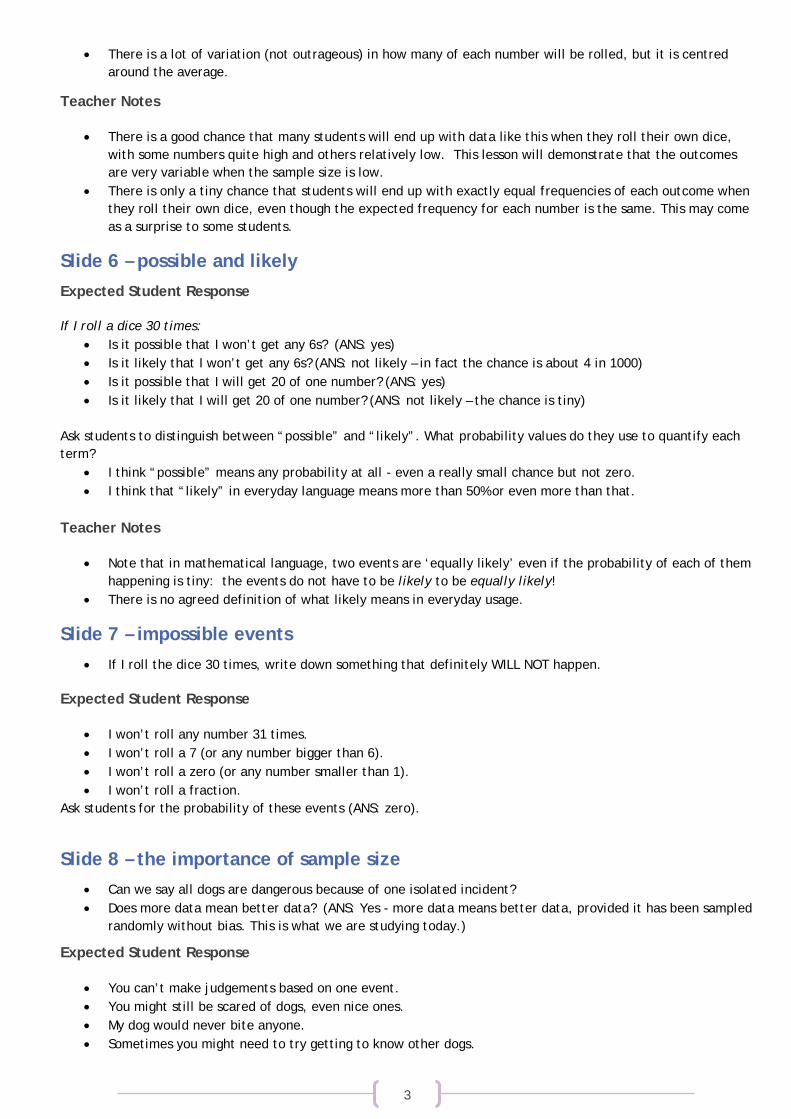
Slide 4 and 5 – common misconceptions
Teacher Notes
• Slide 4 identifies the misconception that 6 is a difficult number to roll on a dice. A related misconception some students have is that because 6 is “difficult”, then 1 must be easy.
• Slide 5 prompts students to consider what evidence is provided by rolling dice.
Expected Student Response
Do you agree with the two students? (first Slide 4 then Slide 5)
• I do not think that 6 was really “harder” to roll – I think 6 was just unlucky this time. • Even if some number got rolled more often than others, that doesn’t make it easy – it’s just probability and
chance. Each time you roll the dice, every number has an equal chance of getting rolled.
3
• There is a lot of variation (not outrageous) in how many of each number will be rolled, but it is centred around the average.
Teacher Notes
• There is a good chance that many students will end up with data like this when they roll their own dice, with some numbers quite high and others relatively low. This lesson will demonstrate that the outcomes are very variable when the sample size is low.
• There is only a tiny chance that students will end up with exactly equal frequencies of each outcome when they roll their own dice, even though the expected frequency for each number is the same. This may come as a surprise to some students.
Slide 6 – possible and likely Expected Student Response
If I roll a dice 30 times: • Is it possible that I won’t get any 6s? (ANS: yes) • Is it likely that I won’t get any 6s? (ANS: not likely – in fact the chance is about 4 in 1000) • Is it possible that I will get 20 of one number? (ANS: yes) • Is it likely that I will get 20 of one number? (ANS: not likely – the chance is tiny)
Ask students to distinguish between “possible” and “likely”. What probability values do they use to quantify each term?
• I think “possible” means any probability at all - even a really small chance but not zero. • I think that “likely” in everyday language means more than 50% or even more than that.
Teacher Notes
• Note that in mathematical language, two events are ‘equally likely’ even if the probability of each of them happening is tiny: the events do not have to be likely to be equally likely!
• There is no agreed definition of what likely means in everyday usage.
Slide 7 – impossible events • If I roll the dice 30 times, write down something that definitely WILL NOT happen.
Expected Student Response
• I won’t roll any number 31 times. • I won’t roll a 7 (or any number bigger than 6). • I won’t roll a zero (or any number smaller than 1). • I won’t roll a fraction.
Ask students for the probability of these events (ANS: zero).
Slide 8 – the importance of sample size • Can we say all dogs are dangerous because of one isolated incident? • Does more data mean better data? (ANS: Yes - more data means better data, provided it has been sampled
randomly without bias. This is what we are studying today.)
Expected Student Response
• You can’t make judgements based on one event. • You might still be scared of dogs, even nice ones. • My dog would never bite anyone. • Sometimes you might need to try getting to know other dogs.
4
• You need to make sure you ask a wide selection of people. If it is not a wide selection, you might have 1000 people who were all bitten by dogs when they were little.
Slide 9 – investigating with dice • If you rolled a six-sided dice 30 times, approximately how many times would you get a 6?
Expected Student Response
• 30 ÷ 6 = 5 so I would predict each number coming up approximately 5 times. • I would expect less 6s than other numbers because 6 is really hard to roll. • I would expect lots of 3s and 4s because they are near the middle of the range 1-6.
Teacher Notes
• This is a good place to link back to Lesson 1 - Four-tunate Fours, and the conversation that we expected to roll a 4 one sixth of the time: this is what the probability of 1/6 means.
• Getting students to commit to an expectation helps to engage them in the lesson. If they have an investment in a particular outcome, they will be keen to test their theory.
• Equally important is to get the students to say why they made their predictions, as in the examples above. Even if their logic is flawed or unreliable, it will useful to see what the thinking is behind their prediction, and to motivate the investigation.
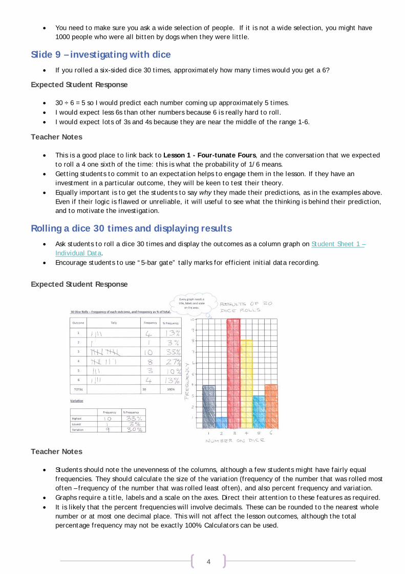
Rolling a dice 30 times and displaying results • Ask students to roll a dice 30 times and display the outcomes as a column graph on Student Sheet 1 –
Individual Data. • Encourage students to use “5-bar gate” tally marks for efficient initial data recording.
Expected Student Response
Teacher Notes
• Students should note the unevenness of the columns, although a few students might have fairly equal frequencies. They should calculate the size of the variation (frequency of the number that was rolled most often – frequency of the number that was rolled least often), and also percent frequency and variation.
• Graphs require a title, labels and a scale on the axes. Direct their attention to these features as required. • It is likely that the percent frequencies will involve decimals. These can be rounded to the nearest whole
number or at most one decimal place. This will not affect the lesson outcomes, although the total percentage frequency may not be exactly 100%. Calculators can be used.
5
Investigating Bigger Samples
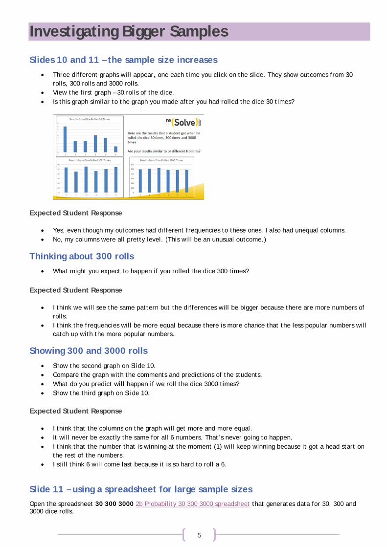
Slides 10 and 11 – the sample size increases • Three different graphs will appear, one each time you click on the slide. They show outcomes from 30
rolls, 300 rolls and 3000 rolls. • View the first graph – 30 rolls of the dice. • Is this graph similar to the graph you made after you had rolled the dice 30 times?
Expected Student Response
• Yes, even though my outcomes had different frequencies to these ones, I also had unequal columns. • No, my columns were all pretty level. (This will be an unusual outcome.)
Thinking about 300 rolls • What might you expect to happen if you rolled the dice 300 times?
Expected Student Response
• I think we will see the same pattern but the differences will be bigger because there are more numbers of rolls.
• I think the frequencies will be more equal because there is more chance that the less popular numbers will catch up with the more popular numbers.
Showing 300 and 3000 rolls • Show the second graph on Slide 10. • Compare the graph with the comments and predictions of the students. • What do you predict will happen if we roll the dice 3000 times? • Show the third graph on Slide 10.
Expected Student Response
• I think that the columns on the graph will get more and more equal. • It will never be exactly the same for all 6 numbers. That’s never going to happen. • I think that the number that is winning at the moment (1) will keep winning because it got a head start on
the rest of the numbers. • I still think 6 will come last because it is so hard to roll a 6.
Slide 11 – using a spreadsheet for large sample sizes Open the spreadsheet 30 300 3000 2b Probability 30 300 3000 spreadsheet that generates data for 30, 300 and 3000 dice rolls.
6
• Show students how data can be generated on the spreadsheet by clicking ctrl=. • Do several trials with each set so that students can see what is happening to the display looking at the
frequencies, frequency as a percent, and the size of the variation in both. • Observe the changes between the results as the sample size gets bigger:
o The relative frequencies (frequencies as percent of the total number of rolls) all get close to 16.67%, the theoretical probability of getting any particular outcome.
o The variation in the relative frequencies gets smaller as sample increases (for 3000 trials it is usually under 3%).
o Because of this, the visual column variation decreases as sample size increases. o The actual frequencies do NOT get closer to each other.
• This behaviour is part of “the law of large numbers”. When the sample size is large and the sample is properly chosen, the percent frequency of an event in the sample is close to the probability of the event.
Teacher Notes
• Prompt the students to use the correct language when talking about probability. • Ask students to explain what they mean and give reasons for their predictions. What do they mean by
“popular numbers”? What do they mean by “catch up”? • Students need to recognise that increasing sample size is an important step in dealing with data. There is a
danger in making predictions based on a small sample size. • An important point to notice is that while increasing a sample size causes the variation to shrink as a
percentage of the overall sample, the actual range of the variation increases in raw numbers. This means that we are more likely to get exactly five tails if we toss a coin ten times than we are to get exactly 500 tails if we toss the coin 1000 times.
• The numbers 30, 300, and 3000 have been chosen specifically because they are all easily divisible by 6, the number of possible outcomes for our experiment. This choice (30, 300, 3000) will mean that when the percentage frequencies are calculated, many of the percentages will be recurring decimals.
• The data for each graph is different. The data for the first 30 rolls is discarded and a new 300 rolls (or 3000 rolls) are done for the next set of tables. The virtual dice is rolled again every time.
• The dice rolls are only shown on one worksheet. For the 30, 300 and 3000 trials the actual dice rolls have been hidden. They are in Column A in a font colour that matches the background colour. You can view them by changing the font colour in that column to a different colour or by changing the background colour for that column and expanding the width of the column.
Pooling the Data Pooling individual 30 rolls data into a class set
• Invite all students to record their frequencies for 30 rolls from Student Sheet 1 – Individual Data on a table on the board.
• Ask students to add up the total frequency for each outcome. • Students use this data to complete Student Sheet 2 – Class Data and write a summary comment comparing
the frequencies and variation in the small and larger data sets. • End with a review of the main findings about how increasing the sample size influences the frequency of
each outcome, the percent frequency and the variation (the law of large numbers). • Student reflections can be recorded on Student Sheet 3 – Reflection 30 300 3000.
Teacher Notes
• The students were very keen to see what their class results would look like after they had seen the spreadsheet that generated 300 and 3000 dice rolls.
• There is still some obvious variation in relative frequency (percent frequency) even when results from 20 students are pooled (so 20 x 30 = 600 dice rolls). Students may note that 600 is closer to 300 than to 3000 rolls. There is still noticeable variation with 3000 rolls.
• Students only need to calculate decimals to one place, or just to the nearest whole number.
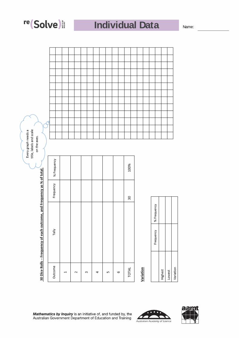
Individual Data Name:
Student Sheet 1 - Individu al Data
Class Data Name:
Student Sheet 2 – Class Data
Reflection 30 300 3000 Name:
Student Sheet 3 – Reflection 30 300 3000
Write down two things that you observe about the graph for your individual data.
1. ____________________________________________________________________________________________
____________________________________________________________________________________________
2. ____________________________________________________________________________________________
____________________________________________________________________________________________
What do you observe when you compare the data and graphs from your personal 30 rolls with the class data?
___________________________________________________________________________________________________
___________________________________________________________________________________________________
___________________________________________________________________________________________________
___________________________________________________________________________________________________
When you look at data, why is important to know the size of the sample it was taken from?
___________________________________________________________________________________________________
___________________________________________________________________________________________________
___________________________________________________________________________________________________
___________________________________________________________________________________________________
Why is this lesson called 30 300 3000?
___________________________________________________________________________________________________
___________________________________________________________________________________________________
___________________________________________________________________________________________________
___________________________________________________________________________________________________
Other comments about what you have discovered:
___________________________________________________________________________________________________
___________________________________________________________________________________________________
___________________________________________________________________________________________________
___________________________________________________________________________________________________
We value your feedback after this lesson via http://tiny.cc/lesson-feedback
PROBABILITY Lesson 3: Alice Australian Curriculum: Mathematics – Year 6 ACMSP144: Describe probabilities using fractions, decimals and percentages.
ACMSP146: Compare observed frequencies across experiments with expected frequencies.
Lesson abstract The task is to predict the number of times selected letters occur in the first 5000 letters from “Alice in Wonderland”. Students take samples from which to predict the number of times selected letters occur. From observed frequencies in the sample, they calculate relative frequencies as fractions, decimals and percent. They use the percent frequency to make the prediction of real frequency in all 5000 letters. They stop when they think the sample is large enough for the prediction to be reliable, and then compare with the actual distribution.
Mathematical purpose (for students) To make good predictions by collecting a sample, the sample has to be a random sample and sufficiently large.
Mathematical purpose (for teachers) This lesson builds on the important ideas from Lesson 2 on probability 30 300 3000. That lesson demonstrated that the more times a dice is thrown, the closer the percent frequency calculated from the experiment is likely to be to the real probability (in that case 1/6). This important phenomenon, part of the ‘law of large numbers’, is the basis of surveys. In this lesson this idea is used in reverse: students find the percent frequency of vowels (for example) in a sample from the text, and if the sample is random and large enough, we can assume that it is close to the real probability. Students calculate the percent frequencies progressively (as fractions, decimals and percent) as their sample size grows, and use the results to predict the number of vowels in the entire text. Finally, students compare their predictions against the actual number and reflect on their method.
At the end of this lesson, students will be able to:
• Collect a random data sample. • Make predictions about a population based on their sample.
Lesson Length 90 minutes approximately
Vocabulary Encountered
• survey • sample • bias • population
Lesson Materials
• Student Sheet 1 - Selection from Alice in Wonderland (2 pages, 1 per student)
• Student Sheet 2 – “Alice” Data Collection (1 per student) • Student Sheet 3 - Checking the Accuracy of the Survey (1 per
student) • Calculators as desired
2
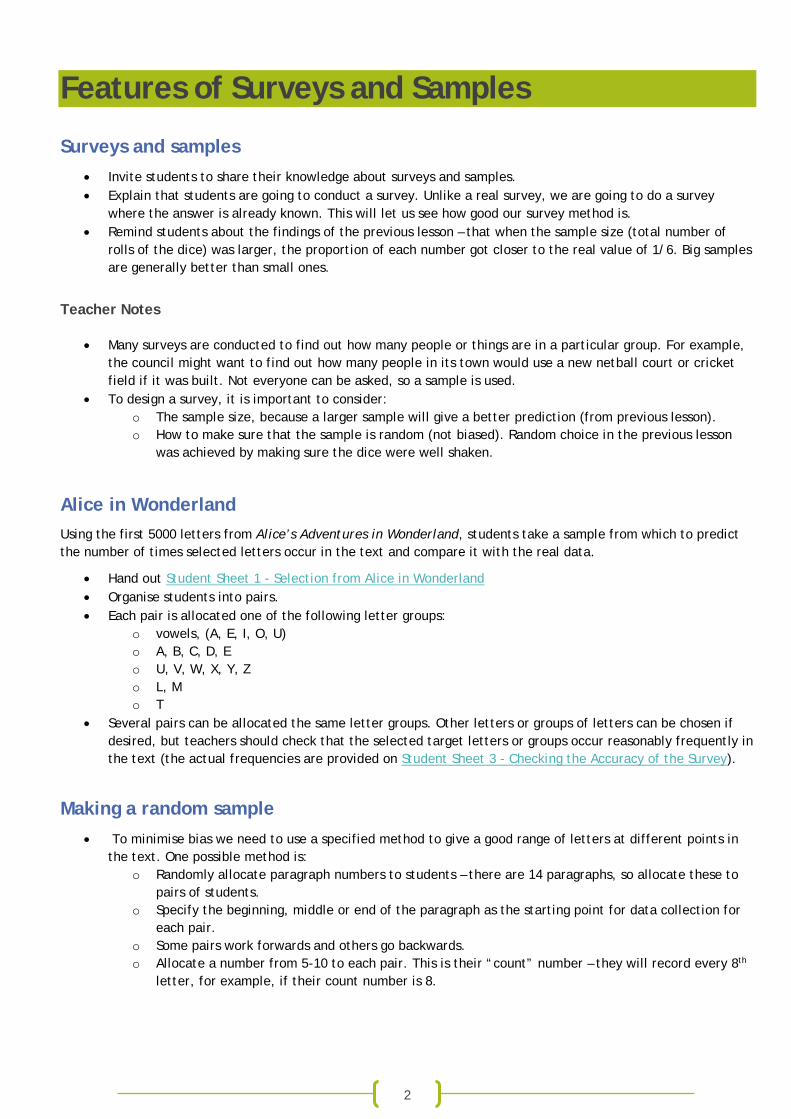
Features of Surveys and Samples
Surveys and samples • Invite students to share their knowledge about surveys and samples. • Explain that students are going to conduct a survey. Unlike a real survey, we are going to do a survey
where the answer is already known. This will let us see how good our survey method is. • Remind students about the findings of the previous lesson – that when the sample size (total number of
rolls of the dice) was larger, the proportion of each number got closer to the real value of 1/6. Big samples are generally better than small ones.
Teacher Notes
• Many surveys are conducted to find out how many people or things are in a particular group. For example, the council might want to find out how many people in its town would use a new netball court or cricket field if it was built. Not everyone can be asked, so a sample is used.
• To design a survey, it is important to consider: o The sample size, because a larger sample will give a better prediction (from previous lesson). o How to make sure that the sample is random (not biased). Random choice in the previous lesson
was achieved by making sure the dice were well shaken.
Alice in Wonderland Using the first 5000 letters from Alice’s Adventures in Wonderland, students take a sample from which to predict the number of times selected letters occur in the text and compare it with the real data.
• Hand out Student Sheet 1 - Selection from Alice in Wonderland • Organise students into pairs. • Each pair is allocated one of the following letter groups:
o vowels, (A, E, I, O, U) o A, B, C, D, E o U, V, W, X, Y, Z o L, M o T
• Several pairs can be allocated the same letter groups. Other letters or groups of letters can be chosen if desired, but teachers should check that the selected target letters or groups occur reasonably frequently in the text (the actual frequencies are provided on Student Sheet 3 - Checking the Accuracy of the Survey).
Making a random sample • To minimise bias we need to use a specified method to give a good range of letters at different points in
the text. One possible method is: o Randomly allocate paragraph numbers to students – there are 14 paragraphs, so allocate these to
pairs of students. o Specify the beginning, middle or end of the paragraph as the starting point for data collection for
each pair. o Some pairs work forwards and others go backwards. o Allocate a number from 5-10 to each pair. This is their “count” number – they will record every 8th
letter, for example, if their count number is 8.
3
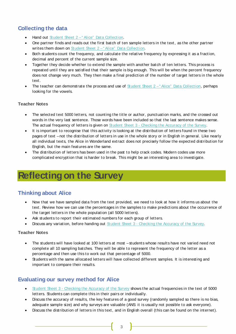
Collecting the data • Hand out Student Sheet 2 – “Alice” Data Collection. • One partner finds and reads out the first batch of ten sample letters in the text, as the other partner
writes them down on Student Sheet 2 – “Alice” Data Collection. • Both students count the frequency, and calculate the relative frequency by expressing it as a fraction,
decimal and percent of the current sample size. • Together they decide whether to extend the sample with another batch of ten letters. This process is
repeated until they are satisfied that their sample is big enough. This will be when the percent frequency does not change very much. They then make a final prediction of the number of target letters in the whole text.
• The teacher can demonstrate the process and use of Student Sheet 2 – “Alice” Data Collection, perhaps looking for the vowels.
Teacher Notes
• The selected text 5000 letters, not counting the title or author, punctuation marks, and the crossed out words in the very last sentence. Those words have been included so that the last sentence makes sense. The actual frequency of letters is given on Student Sheet 3 - Checking the Accuracy of the Survey.
• It is important to recognise that this activity is looking at the distribution of letters found in these two pages of text – not the distribution of letters in use in the whole story or in English in general. Like nearly all individual texts, the Alice in Wonderland extract does not precisely follow the expected distribution for English, but the main features are the same.
• The distribution of letters has been used in the past to help crack codes. Modern codes use more complicated encryption that is harder to break. This might be an interesting area to investigate.
Reflecting on the Survey
Thinking about Alice • Now that we have sampled data from the text provided, we need to look at how it informs us about the
text. Review how we can use the percentages in the samples to make predictions about the occurrence of the target letters in the whole population (all 5000 letters).
• Ask students to report their estimated numbers for each group of letters. • Discuss any variation, before handing out Student Sheet 3 - Checking the Accuracy of the Survey.
Teacher Notes
• The students will have looked at 100 letters at most – students whose results have not varied need not complete all 10 sampling batches. They will be able to represent the frequency of the letter as a percentage and then use this to work out that percentage of 5000.
• Students with the same allocated letters will have collected different samples. It is interesting and important to compare their results.
Evaluating our survey method for Alice • Student Sheet 3 - Checking the Accuracy of the Survey shows the actual frequencies in the text of 5000
letters. Students can complete this in their pairs or individually. • Discuss the accuracy of results, the key features of a good survey (randomly sampled so there is no bias,
adequate sample size) and why surveys are valuable (ANS: it is usually not possible to ask everyone). • Discuss the distribution of letters in this text, and in English overall (this can be found on the internet).
4
Teacher Notes
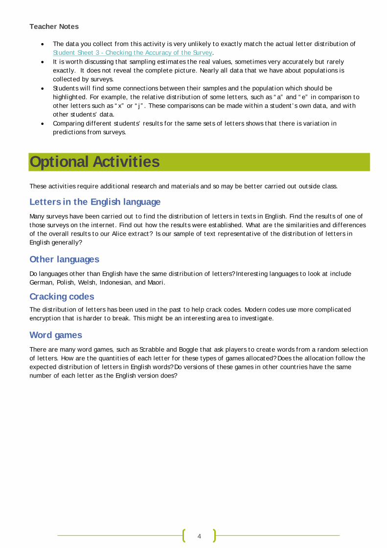
• The data you collect from this activity is very unlikely to exactly match the actual letter distribution of Student Sheet 3 - Checking the Accuracy of the Survey.
• It is worth discussing that sampling estimates the real values, sometimes very accurately but rarely exactly. It does not reveal the complete picture. Nearly all data that we have about populations is collected by surveys.
• Students will find some connections between their samples and the population which should be highlighted. For example, the relative distribution of some letters, such as “a” and “e” in comparison to other letters such as “x” or “j”. These comparisons can be made within a student’s own data, and with other students’ data.
• Comparing different students’ results for the same sets of letters shows that there is variation in predictions from surveys.
Optional Activities
These activities require additional research and materials and so may be better carried out outside class.
Letters in the English language Many surveys have been carried out to find the distribution of letters in texts in English. Find the results of one of those surveys on the internet. Find out how the results were established. What are the similarities and differences of the overall results to our Alice extract? Is our sample of text representative of the distribution of letters in English generally?
Other languages Do languages other than English have the same distribution of letters? Interesting languages to look at include German, Polish, Welsh, Indonesian, and Maori.
Cracking codes The distribution of letters has been used in the past to help crack codes. Modern codes use more complicated encryption that is harder to break. This might be an interesting area to investigate.
Word games There are many word games, such as Scrabble and Boggle that ask players to create words from a random selection of letters. How are the quantities of each letter for these types of games allocated? Does the allocation follow the expected distribution of letters in English words? Do versions of these games in other countries have the same number of each letter as the English version does?
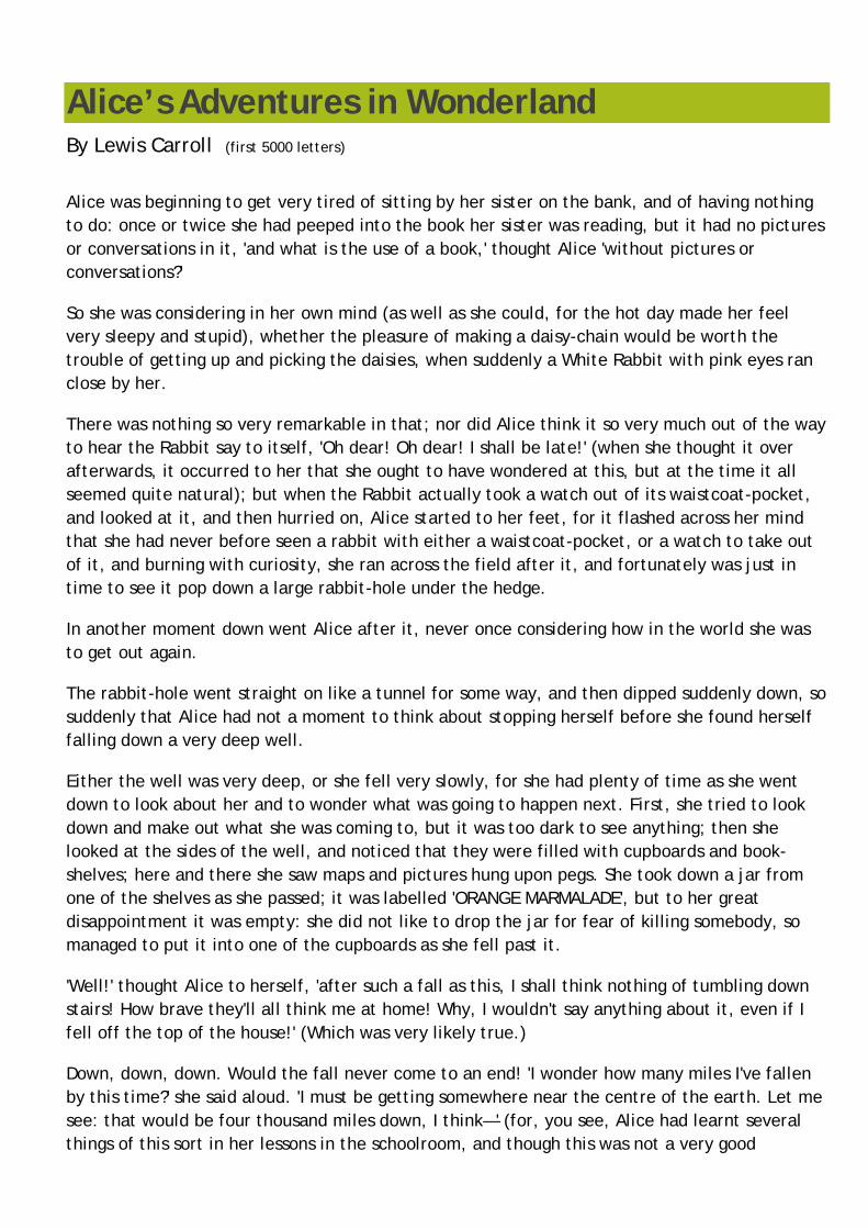
Alice’s Adventures in Wonderland Student Sheet 1 – Selection f rom Alice in Wonderland
By Lewis Carroll (first 5000 letters)
Alice was beginning to get very tired of sitting by her sister on the bank, and of having nothing to do: once or twice she had peeped into the book her sister was reading, but it had no pictures or conversations in it, 'and what is the use of a book,' thought Alice 'without pictures or conversations?'
So she was considering in her own mind (as well as she could, for the hot day made her feel very sleepy and stupid), whether the pleasure of making a daisy-chain would be worth the trouble of getting up and picking the daisies, when suddenly a White Rabbit with pink eyes ran close by her.
There was nothing so very remarkable in that; nor did Alice think it so very much out of the way to hear the Rabbit say to itself, 'Oh dear! Oh dear! I shall be late!' (when she thought it over afterwards, it occurred to her that she ought to have wondered at this, but at the time it all seemed quite natural); but when the Rabbit actually took a watch out of its waistcoat-pocket, and looked at it, and then hurried on, Alice started to her feet, for it flashed across her mind that she had never before seen a rabbit with either a waistcoat-pocket, or a watch to take out of it, and burning with curiosity, she ran across the field after it, and fortunately was just in time to see it pop down a large rabbit-hole under the hedge.
In another moment down went Alice after it, never once considering how in the world she was to get out again.
The rabbit-hole went straight on like a tunnel for some way, and then dipped suddenly down, so suddenly that Alice had not a moment to think about stopping herself before she found herself falling down a very deep well.
Either the well was very deep, or she fell very slowly, for she had plenty of time as she went down to look about her and to wonder what was going to happen next. First, she tried to look down and make out what she was coming to, but it was too dark to see anything; then she looked at the sides of the well, and noticed that they were filled with cupboards and book-shelves; here and there she saw maps and pictures hung upon pegs. She took down a jar from one of the shelves as she passed; it was labelled 'ORANGE MARMALADE', but to her great disappointment it was empty: she did not like to drop the jar for fear of killing somebody, so managed to put it into one of the cupboards as she fell past it.
'Well!' thought Alice to herself, 'after such a fall as this, I shall think nothing of tumbling down stairs! How brave they'll all think me at home! Why, I wouldn't say anything about it, even if I fell off the top of the house!' (Which was very likely true.)
Down, down, down. Would the fall never come to an end! 'I wonder how many miles I've fallen by this time?' she said aloud. 'I must be getting somewhere near the centre of the earth. Let me see: that would be four thousand miles down, I think—' (for, you see, Alice had learnt several things of this sort in her lessons in the schoolroom, and though this was not a very good
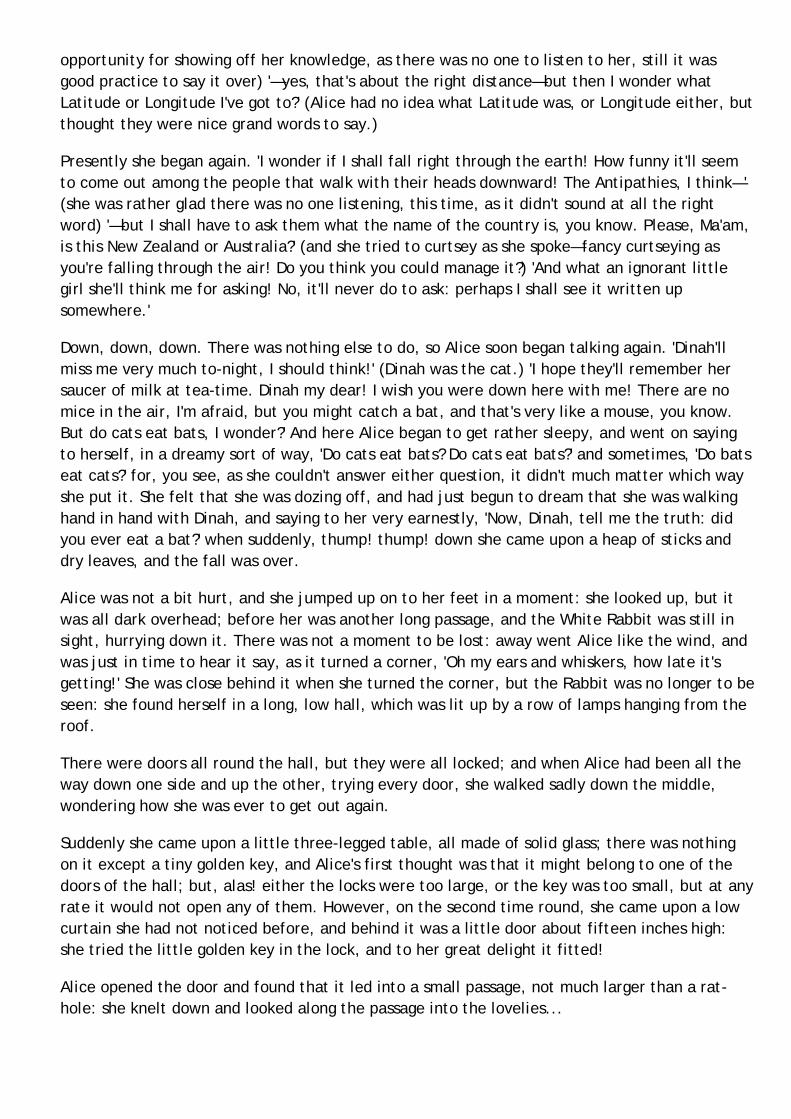
opportunity for showing off her knowledge, as there was no one to listen to her, still it was good practice to say it over) '—yes, that's about the right distance—but then I wonder what Latitude or Longitude I've got to?' (Alice had no idea what Latitude was, or Longitude either, but thought they were nice grand words to say.)
Presently she began again. 'I wonder if I shall fall right through the earth! How funny it'll seem to come out among the people that walk with their heads downward! The Antipathies, I think—' (she was rather glad there was no one listening, this time, as it didn't sound at all the right word) '—but I shall have to ask them what the name of the country is, you know. Please, Ma'am, is this New Zealand or Australia?' (and she tried to curtsey as she spoke—fancy curtseying as you're falling through the air! Do you think you could manage it?) 'And what an ignorant little girl she'll think me for asking! No, it'll never do to ask: perhaps I shall see it written up somewhere.'
Down, down, down. There was nothing else to do, so Alice soon began talking again. 'Dinah'll miss me very much to-night, I should think!' (Dinah was the cat.) 'I hope they'll remember her saucer of milk at tea-time. Dinah my dear! I wish you were down here with me! There are no mice in the air, I'm afraid, but you might catch a bat, and that's very like a mouse, you know. But do cats eat bats, I wonder?' And here Alice began to get rather sleepy, and went on saying to herself, in a dreamy sort of way, 'Do cats eat bats? Do cats eat bats?' and sometimes, 'Do bats eat cats?' for, you see, as she couldn't answer either question, it didn't much matter which way she put it. She felt that she was dozing off, and had just begun to dream that she was walking hand in hand with Dinah, and saying to her very earnestly, 'Now, Dinah, tell me the truth: did you ever eat a bat?' when suddenly, thump! thump! down she came upon a heap of sticks and dry leaves, and the fall was over.
Alice was not a bit hurt, and she jumped up on to her feet in a moment: she looked up, but it was all dark overhead; before her was another long passage, and the White Rabbit was still in sight, hurrying down it. There was not a moment to be lost: away went Alice like the wind, and was just in time to hear it say, as it turned a corner, 'Oh my ears and whiskers, how late it's getting!' She was close behind it when she turned the corner, but the Rabbit was no longer to be seen: she found herself in a long, low hall, which was lit up by a row of lamps hanging from the roof.
There were doors all round the hall, but they were all locked; and when Alice had been all the way down one side and up the other, trying every door, she walked sadly down the middle, wondering how she was ever to get out again.
Suddenly she came upon a little three-legged table, all made of solid glass; there was nothing on it except a tiny golden key, and Alice's first thought was that it might belong to one of the doors of the hall; but, alas! either the locks were too large, or the key was too small, but at any rate it would not open any of them. However, on the second time round, she came upon a low curtain she had not noticed before, and behind it was a little door about fifteen inches high: she tried the little golden key in the lock, and to her great delight it fitted!
Alice opened the door and found that it led into a small passage, not much larger than a rat-hole: she knelt down and looked along the passage into the lovelies...
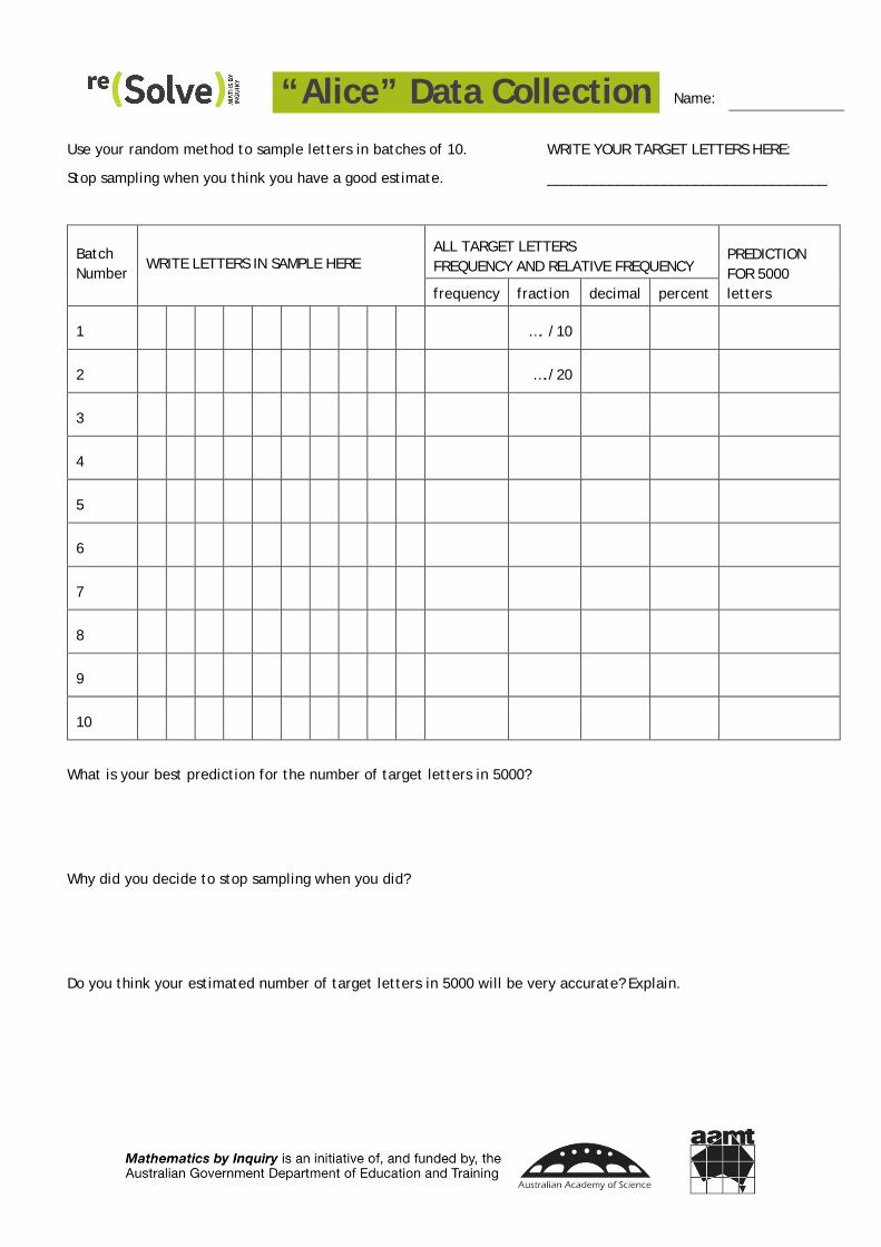
“Alice” Data Collection Name:
Student Sheet 2 – “ Alice” Data Collection
Use your random method to sample letters in batches of 10. WRITE YOUR TARGET LETTERS HERE:
Stop sampling when you think you have a good estimate. ____________________________________
Batch Number
WRITE LETTERS IN SAMPLE HERE ALL TARGET LETTERS FREQUENCY AND RELATIVE FREQUENCY
PREDICTION FOR 5000 letters frequency fraction decimal percent
1 …. /10
2 …./20
3
4
5
6
7
8
9
10
What is your best prediction for the number of target letters in 5000?
Why did you decide to stop sampling when you did?
Do you think your estimated number of target letters in 5000 will be very accurate? Explain.
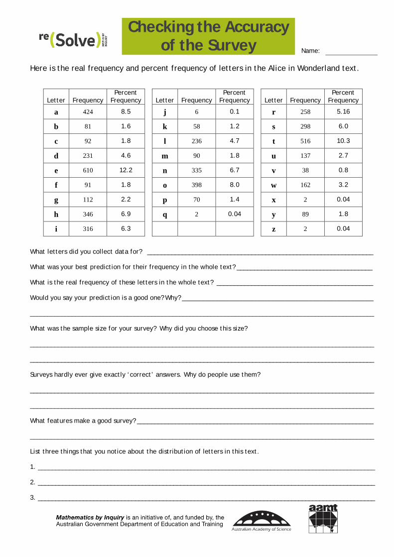
Checking the Accuracy of the Survey Name:
Student Sheet 3 – Checking the Accuracy of the Survey
Here is the real frequency and percent frequency of letters in the Alice in Wonderland text.
Letter Frequency Percent
Frequency Letter Frequency Percent
Frequency Letter Frequency Percent
Frequency
a 424 8.5 j 6 0.1 r 258 5.16
b 81 1.6 k 58 1.2 s 298 6.0
c 92 1.8 l 236 4.7 t 516 10.3
d 231 4.6 m 90 1.8 u 137 2.7
e 610 12.2 n 335 6.7 v 38 0.8
f 91 1.8 o 398 8.0 w 162 3.2
g 112 2.2 p 70 1.4 x 2 0.04
h 346 6.9 q 2 0.04 y 89 1.8
i 316 6.3 z 2 0.04
What letters did you collect data for? _________________________________________________________________
What was your best prediction for their frequency in the whole text? _______________________________________
What is the real frequency of these letters in the whole text? _____________________________________________
Would you say your prediction is a good one? Why? _______________________________________________________
___________________________________________________________________________________________________
What was the sample size for your survey? Why did you choose this size?
___________________________________________________________________________________________________
___________________________________________________________________________________________________
Surveys hardly ever give exactly ‘correct’ answers. Why do people use them?
___________________________________________________________________________________________________
___________________________________________________________________________________________________
What features make a good survey? ____________________________________________________________________
___________________________________________________________________________________________________
List three things that you notice about the distribution of letters in this text.
1. _________________________________________________________________________________________________
2. _________________________________________________________________________________________________
3. _________________________________________________________________________________________________
We value your feedback after this lesson via http://tiny.cc/lesson-feedback
PROBABILITY Lesson 4: Plenty More Fish in the Sea Australian Curriculum: Mathematics – Year 6 ACMSP144: Describe probabilities using fractions, decimals and percentages. ACMSP145: Conduct chance experiments with both small and large numbers of trials using appropriate digital technologies. ACMSP146: Compare observed frequencies across experiments with expected frequencies.
Lesson abstract Students gather data about a population by sampling. They start in a whole class introduction with a small set of unseen counters in a bag and work out the proportion of colours in the bag by sampling and replacing. ‘Tagged fish’ are introduced into the bag so that the numbers of counters in the bag can be estimated. This method is then applied to estimate the population of the school playground by releasing students as ‘tagged fish’ at break time.
Mathematical purpose (for students) To learn how the size of populations can be estimated.
Mathematical purpose (for teachers) Students engage in a practical experience of the important capture-mark-recapture method of estimating animal populations. In doing this, students apply the central idea of reSolve lesson 30 300 3000 that the probabilities related to a whole population can be estimated by the relative frequencies (e.g. percent frequencies) calculated from a good sample.
At the end of this lesson, students will be able to:
• Use sampling to estimate the composition of a population. • Recall the importance of sample size when collecting data. • Appreciate one way in which mathematics is used in environmental science.
Lesson Length 90 minutes approximately
Vocabulary Encountered
• survey • sample • population • fish tagging
Lesson Materials
• bag from which to draw counters • 18 red counters, 9 blue counters, 3 yellow counters • Student Sheet 1 – What’s in the Bag? (1 per student)
2
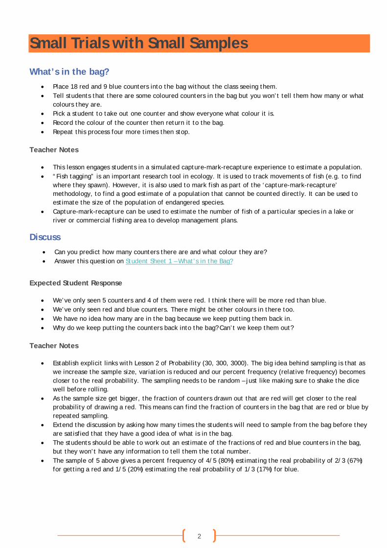
Small Trials with Small Samples
What’s in the bag? • Place 18 red and 9 blue counters into the bag without the class seeing them. • Tell students that there are some coloured counters in the bag but you won’t tell them how many or what
colours they are. • Pick a student to take out one counter and show everyone what colour it is. • Record the colour of the counter then return it to the bag. • Repeat this process four more times then stop.
Teacher Notes
• This lesson engages students in a simulated capture-mark-recapture experience to estimate a population. • “Fish tagging” is an important research tool in ecology. It is used to track movements of fish (e.g. to find
where they spawn). However, it is also used to mark fish as part of the ‘capture-mark-recapture’ methodology, to find a good estimate of a population that cannot be counted directly. It can be used to estimate the size of the population of endangered species.
• Capture-mark-recapture can be used to estimate the number of fish of a particular species in a lake or river or commercial fishing area to develop management plans.
Discuss • Can you predict how many counters there are and what colour they are? • Answer this question on Student Sheet 1 – What’s in the Bag?
Expected Student Response
• We’ve only seen 5 counters and 4 of them were red. I think there will be more red than blue. • We’ve only seen red and blue counters. There might be other colours in there too. • We have no idea how many are in the bag because we keep putting them back in. • Why do we keep putting the counters back into the bag? Can’t we keep them out?
Teacher Notes
• Establish explicit links with Lesson 2 of Probability (30, 300, 3000). The big idea behind sampling is that as we increase the sample size, variation is reduced and our percent frequency (relative frequency) becomes closer to the real probability. The sampling needs to be random – just like making sure to shake the dice well before rolling.
• As the sample size get bigger, the fraction of counters drawn out that are red will get closer to the real probability of drawing a red. This means can find the fraction of counters in the bag that are red or blue by repeated sampling.
• Extend the discussion by asking how many times the students will need to sample from the bag before they are satisfied that they have a good idea of what is in the bag.
• The students should be able to work out an estimate of the fractions of red and blue counters in the bag, but they won’t have any information to tell them the total number.
• The sample of 5 above gives a percent frequency of 4/5 (80%) estimating the real probability of 2/3 (67%) for getting a red and 1/5 (20%) estimating the real probability of 1/3 (17%) for blue.
3
Tag and test • How can we find out how many counters are in the bag? So far, we have no information. • Show students 3 yellow counters. These counters are going to be our “tagged fish” that we are going to
“release” into the bag. • Put the yellow counters into the bag. We now know that there are some red, some blue and 3 yellow
counters in the bag. • Draw a counter out of the bag, record the colour, then return it to the bag. • Stop after 10 “captures”. • How many of each colour have we “caught”?
Discuss • Can you predict how many counters are in the bag and what colour they are? • Answer this question on Student Sheet 1 – What’s in the Bag?
Expected Student Response
• Sample student response – “We caught 7 reds, 2 blues and 1 yellow.” • Looks like there are more reds than yellow or blue. • There are 3 yellows in there and I only caught one of them. I caught more than 3 times as many reds. So
there might be about 20 reds in the bag. • One tenth of the counters caught were yellow. So I estimate that the real probability of catching a yellow
was 1/10. There are 3 yellows, so I think there are 30 counters in the bag. • We only caught 10 counters. The variation in small samples means this is not very reliable.
Teacher Notes
• It is quite possible in this simulation of tag and release that you won’t draw out any of your “tagged” (yellow) fish. Increase your sample size.
• Emphasise links to probability and relative frequency (percent or fraction).
Discuss • Would taking more counters out of the bag increase your confidence in your prediction? • Answer this question on Student Sheet 1 – What’s in the Bag?
Expected Student Response
• A bigger sample might be a good idea. Then we could see more of the counters, and it would reduce the element of chance.
• There can’t be too many counters in that bag. I think we have pulled most of them out already so I can’t see what difference it would make to keep going.
4
Estimating the Population of the School
Fishing for the school population • Invite students to apply their knowledge of sampling and fish tagging to estimate the number of students in
their playground at a break time. • You will need 25 students to do this activity (see Teacher Notes). • 20 students from the class will be “tagged fish” and released into the playground at a break time. They will
need to circulate normally around the playground and behave in the ways they normally would. • The remaining 5 students will be the researchers who will collect samples. They each need to find a place
around the school where there will be moderate traffic from across all year levels and classes, so as not to bias the data sample. They might chose a particular doorway, a line on the playground or a crack in the footpath as their data collection point, recording people who pass over or through this designated position.
• It is important that the “tagged fish” do not know where the “researchers” will be or what location they choose as their data collection point.
• Researchers each fix a number to use as their “catching interval”. For example, if their interval number is 6, they record every sixth student who crosses this line, crack, doorway etc. This is to help eliminate bias – for example a whole class of students walking back late from the library may skew the data. The catching intervals need to be fixed in advance of data collection, but also need to be suitable for traffic at that position.
• Researchers only need to record whether the ‘caught’ student is a tagged fish (in their class) or not. • Researchers stop when they get 2 tagged fish. • The same fish may be caught more than once by the researchers. This is not a problem unless the fish
deliberately try to influence the results.
Teacher Notes
• For this activity you need 25 students. If you do not have that many in your class, “borrow” some students from another class to act as tagged fish. Having exactly 20 tagged fish and exactly 10 observations of tagged fish makes the final calculation easier. (See Variation 2 for a statistically stronger method.)
• If you have more than 25 students in your class, some students pair up as “researchers”. • The activity needs to be conducted on either side of a break time:
o Approximately 45 minutes before the break to do the introduction to the lesson and prepare the “tagging” activity
o The recess or lunch break to do the data collecting o Another 45 minutes after the break to calculate, discuss and record the results.
Reporting back • After the break, the researchers report the numbers of untagged fish they caught before getting 2 tagged
fish and report any difficulties with the data collection to the class. • Record results as a table (sample below). • The 10 tagged fish that were caught represent 50% of the total number of tagged fish (20), and so we
estimate that the untagged fish that were caught represent 50% of the playground population. How many students were in the playground?
5
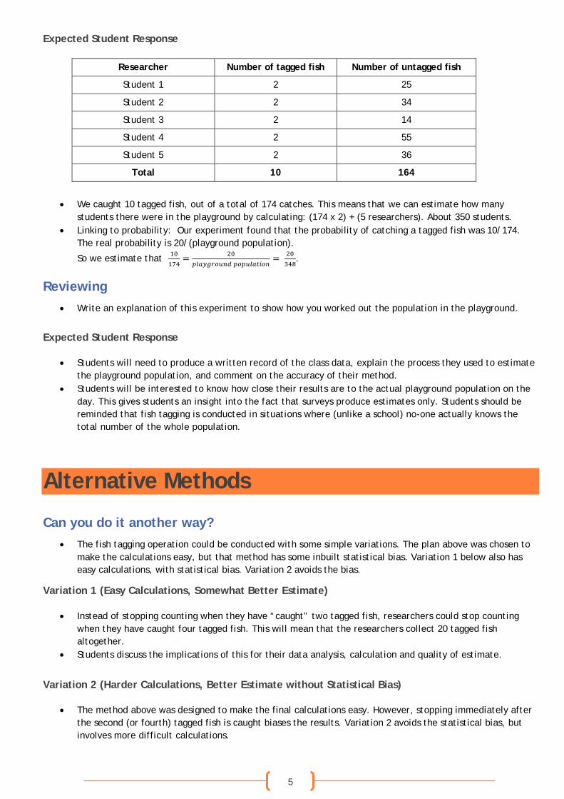
Expected Student Response
Researcher Number of tagged fish Number of untagged fish
Student 1 2 25
Student 2 2 34
Student 3 2 14
Student 4 2 55
Student 5 2 36
Total 10 164
• We caught 10 tagged fish, out of a total of 174 catches. This means that we can estimate how many students there were in the playground by calculating: (174 x 2) + (5 researchers). About 350 students.
• Linking to probability: Our experiment found that the probability of catching a tagged fish was 10/174. The real probability is 20/(playground population).
So we estimate that 10174
= 20𝑝𝑝𝑝𝑝𝑝𝑝𝑝𝑝𝑝𝑝𝑝𝑝𝑝𝑝𝑝𝑝𝑝𝑝𝑝𝑝 𝑝𝑝𝑝𝑝𝑝𝑝𝑝𝑝𝑝𝑝𝑝𝑝𝑝𝑝𝑝𝑝𝑝𝑝𝑝𝑝
= 20348
.
Reviewing • Write an explanation of this experiment to show how you worked out the population in the playground.
Expected Student Response
• Students will need to produce a written record of the class data, explain the process they used to estimate the playground population, and comment on the accuracy of their method.
• Students will be interested to know how close their results are to the actual playground population on the day. This gives students an insight into the fact that surveys produce estimates only. Students should be reminded that fish tagging is conducted in situations where (unlike a school) no-one actually knows the total number of the whole population.
Alternative Methods
Can you do it another way? • The fish tagging operation could be conducted with some simple variations. The plan above was chosen to
make the calculations easy, but that method has some inbuilt statistical bias. Variation 1 below also has easy calculations, with statistical bias. Variation 2 avoids the bias.
Variation 1 (Easy Calculations, Somewhat Better Estimate)
• Instead of stopping counting when they have “caught” two tagged fish, researchers could stop counting when they have caught four tagged fish. This will mean that the researchers collect 20 tagged fish altogether.
• Students discuss the implications of this for their data analysis, calculation and quality of estimate.
Variation 2 (Harder Calculations, Better Estimate without Statistical Bias)
• The method above was designed to make the final calculations easy. However, stopping immediately after the second (or fourth) tagged fish is caught biases the results. Variation 2 avoids the statistical bias, but involves more difficult calculations.
6
• Instead of stopping counting when they have each “caught” two tagged fish, researchers stop counting when they have each caught 20 fish in total, regardless of whether they were tagged or not.
• This will mean that between them, the researchers will have caught 100 fish, some of which will be tagged.
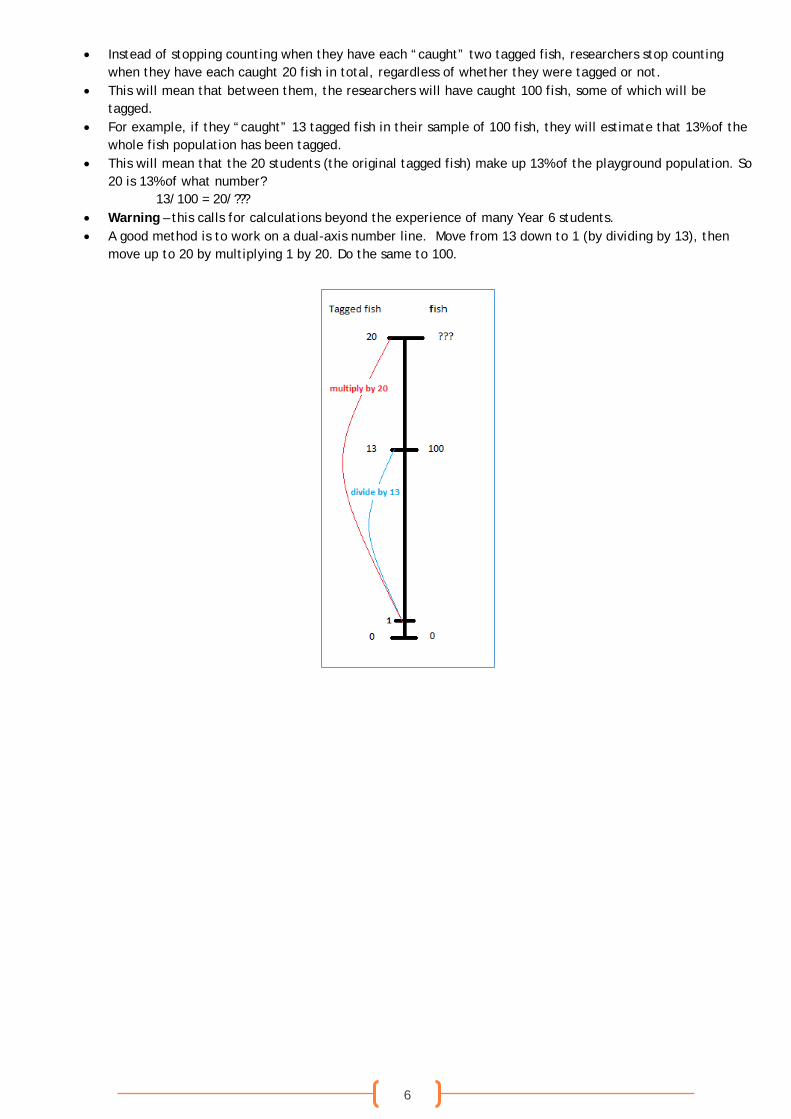
• For example, if they “caught” 13 tagged fish in their sample of 100 fish, they will estimate that 13% of the whole fish population has been tagged.
• This will mean that the 20 students (the original tagged fish) make up 13% of the playground population. So 20 is 13% of what number?
13/100 = 20/??? • Warning – this calls for calculations beyond the experience of many Year 6 students. • A good method is to work on a dual-axis number line. Move from 13 down to 1 (by dividing by 13), then
move up to 20 by multiplying 1 by 20. Do the same to 100.
7
Related Tasks
Spotto • Spotto is a game played by many families in their cars. • The first person to spot a yellow car and yell “Spotto!” gets one point. • Is yellow the least common colour of car on the road? Design a survey to answer this question. • How can you find the probability of seeing a yellow car on the road? • Someone told me that the chance of seeing a yellow car when you are playing Spotto is 1%. Explain
carefully what the person might really mean by this. Do you think it is correct? Give your reasons carefully.
“Yes” cars • All car number plates in the Australian Capital Territory start with the letter “Y”. A popular Canberra
tradition is to spot the “YES” cars, those that have the letters “YES” at the start of their number plate. • How many possible “YES” cars could there be in Canberra if the registration number is made up of 3 letters
followed by 2 numbers then a letter? • What information would you need to work out the probability of seeing one? • What number plate would be good to spot in your part of Australia?
Capture-mark-recapture • Finding out the number of animals that there are in an area is an important part of species conservation
and of responsibly managing resources. • A capture-mark-recapture method, as experienced in this lesson, is often used. • Animals don’t always have to be physically captured or physically marked to use this method. Visual
recognition was used to estimate the number of brumbies in the Australian Alps in 2015. • Find some recent examples in your region or state.
o What animal population was to be estimated? o How was it done? o Why is it important to know how many of these animals there are?
• A famous use of the capture-mark-recapture method was a study by Kettlewell that showed that peppered moths survive better if they blend in with their environment. As pollution increased in the industrial revolution, the proportion of darker peppered moths increased. https://www.biologycorner.com/worksheets/pepperedmoth.html
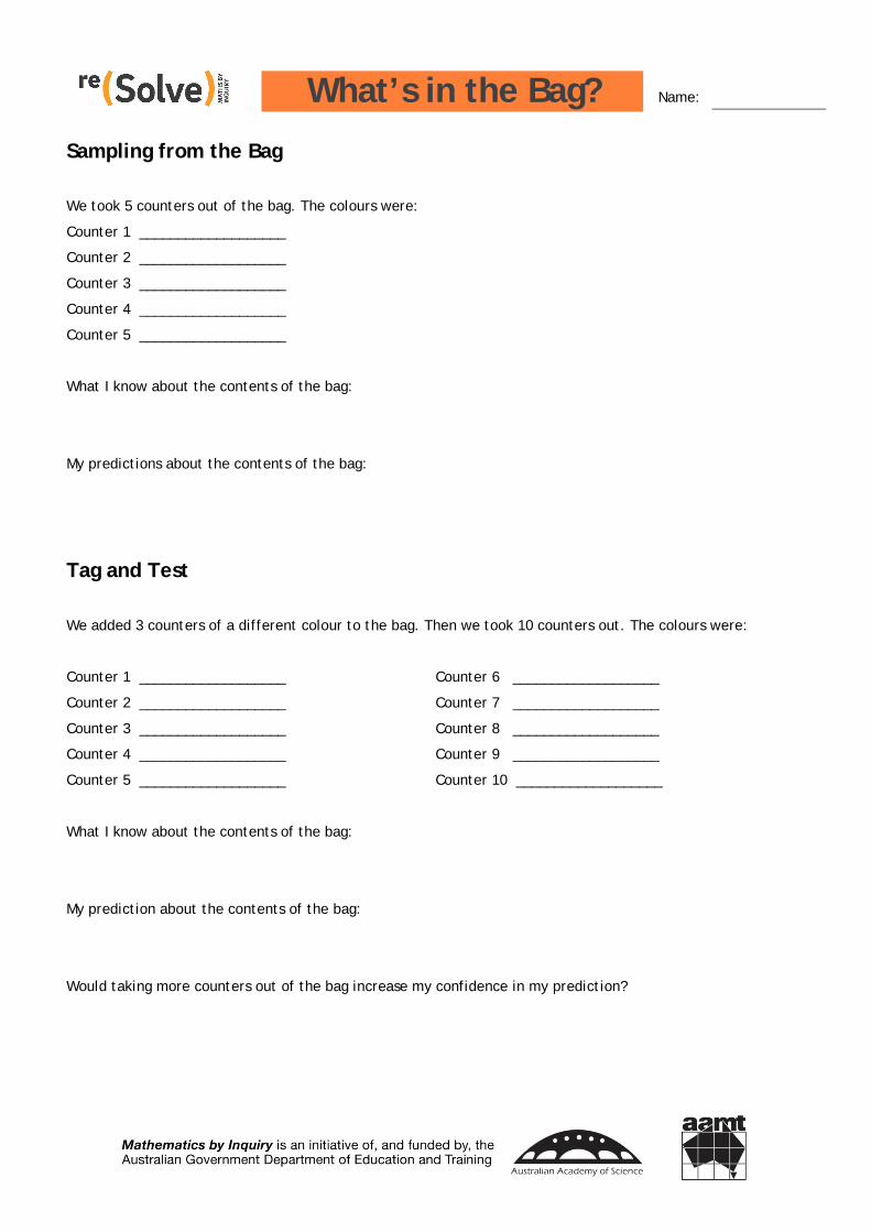
What’s in the Bag? Name:
Student Sheet 1 – What’s in the Bag?
Sampling from the Bag
We took 5 counters out of the bag. The colours were:
Counter 1 ___________________
Counter 2 ___________________
Counter 3 ___________________
Counter 4 ___________________
Counter 5 ___________________
What I know about the contents of the bag:
My predictions about the contents of the bag:
Tag and Test
We added 3 counters of a different colour to the bag. Then we took 10 counters out. The colours were:
Counter 1 ___________________ Counter 6 ___________________
Counter 2 ___________________ Counter 7 ___________________
Counter 3 ___________________ Counter 8 ___________________
Counter 4 ___________________ Counter 9 ___________________
Counter 5 ___________________ Counter 10 ___________________
What I know about the contents of the bag:
My prediction about the contents of the bag:
Would taking more counters out of the bag increase my confidence in my prediction?