Probability Primer

Seungjin Choi

Department of Computer Science and EngineeringPohang University of Science and Technology

77 Cheongam-ro, Nam-gu, Pohang 790-784, Koreaseungjin@postech.ac.kr

http://mlg.postech.ac.kr/∼seungjin

1 / 21

Why Probability?

Machine learning deals with uncertain quantities or stochasticquantities.

Sources of uncertainty:

I Inherent stochasticity in the system being modeled

I Incomplete observability

I Incomplete modeling

[Source: Chapter 3 in Deep Learning book by Goodfellow-Bengio-Couville, 2016]

2 / 21

Probabilistic Models in Machine Learning

I A probabilistic model is a joint distribution,

p(x, z),

over observed variables x and hidden variables z.

I Inference about unknowns is carried out by calculating theposterior distribution over hidden variables:

p(z|x) =p(x, z)

p(x).

I The evidence p(x) is not tractable in most of models of interest, weresort to approximate inference. (is NOT covered in this class, willbe handled in CSED 515)

3 / 21

Sets, Fields, Events

I A set is a collection of objects. The objects are called elements ofthe set.

I A sample space Ω is the set of all outcomes of an experiment.

I A subset of Ω is called event. A collection of subsets of Ω are calledevents.

I Consider a universal set Ω and a collection of subsets of Ω. LetE ,F , . . . denote subsets in this collection. This collection of subsetsof Ω forms a field M if

1. ∅ ∈ M, Ω ∈M.2. If E ∈M and F ∈M, then E ∪ F ∈M. and E ∩ F ∈M.3. If E ∈M, then E c ∈M.

I A σ-field F is a field that is closed under any countable set ofunions, intersections, and combinations.

4 / 21

Probability Measure

Given a sample space Ω, a function P defined on the subsets of Ω is aprobability measure if the following four axioms are satisfied:

1. P(A) ≥ 0 for any event A ∈ F .

2. P(∅) = 0.

3. P(Ω) = 1.

4. P(∪∞i=1Ai ) =∑∞

i=1 P(Ai ) if A1,A2, . . . are events that are mutuallyexclusive or pairwise disjoint.

The probability measure P : F 7→ [0, 1] is a function on F that assigns toan event A ∈ F a number in [0,1], such that above axioms are satisfied.

5 / 21

Probability Space

DefinitionA probability space is a triplet (Ω,F ,P) where Ω is a set, F is aσ-algebra, and P is a probability measure on (Ω,F).

A probability space (Ω,F ,P) is a mathematical model of a random experiment,

an experiment whose exact outcome cannot be told in advance. The set Ω

stands for the collection of all possible outcomes of the experiment. A subset F

is said to occur if the outcome of the experiment happens to belong to F .

Given our capabilities to measure, detect, and discern, and given the nature of

answers we seek, only certain subsets F are distinguished enough to be of

concern whether they occur. The σ-algebra F is the collection of all such

subsets whose occurrence are noteworthy and decidable; the elements of F are

called events. From this point of view, the conditions for F to be a σ-algebra

are logical consequences of the interpretation of the term ’event’. Finally, for

each event F , the chances that F occurs is modeled to be the number P(F ),

called the probability that F occurs.

6 / 21

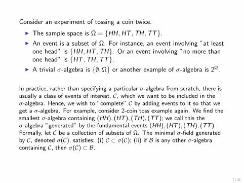
Consider an experiment of tossing a coin twice.

I The sample space is Ω = HH,HT ,TH,TT.I An event is a subset of Ω. For instance, an event involving ”at least

one head” is HH,HT ,TH. Or an event involving ”no more thanone head” is HT ,TH,TT.

I A trivial σ-algebra is ∅,Ω or another example of σ-algebra is 2Ω.

In practice, rather than specifying a particular σ-algebra from scratch, there isusually a class of events of interest, C, which we want to be included in theσ-algebra. Hence, we wish to ”complete” C by adding events to it so that weget a σ-algebra. For example, consider 2-coin toss example again. We find thesmallest σ-algebra containing (HH), (HT ), (TH), (TT ); we call this theσ-algebra ”generated” by the fundamental events (HH), (HT ), (TH), (TT ).Formally, let C be a collection of subsets of Ω. The minimal σ-field generatedby C, denoted σ(C), satisfies: (i) C ⊂ σ(C); (ii) if B is any other σ-algebracontaining C, then σ(C) ⊂ B.

7 / 21

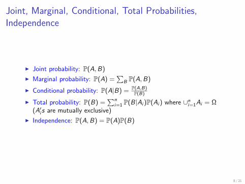
Joint, Marginal, Conditional, Total Probabilities,Independence

I Joint probability: P(A,B)

I Marginal probability: P(A) =∑

B P(A,B)

I Conditional probability: P(A|B) = P(A,B)P(B)

I Total probability: P(B) =∑n

i=1 P(B|Ai )P(Ai ) where ∪ni=1Ai = Ω(A′i s are mutually exclusive)

I Independence: P(A,B) = P(A)P(B)

8 / 21

P(X, Y) P(Y)

P(X)

=

[Figure source: Murphy’s]

9 / 21

Bayes Theorem

Theorem (Bayes’ theorem)Let Ai , i = 1, . . . , n be a set of disjoint and exhaustive events. Then∪ni=1Ai = Ω, Ai ∩ Aj = ∅, i 6= j . For any event B with P(B) > 0 andP(Ai ) 6= 0 ∀i ,

P(Aj |B) =P(B|Aj)P(Aj)

P(B)=

P(B|Aj)P(Aj)∑ni=1 P(B|Ai )P(Ai )

.

10 / 21

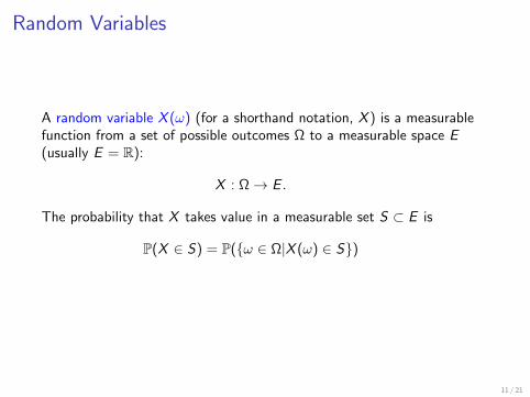
Random Variables

A random variable X (ω) (for a shorthand notation, X ) is a measurablefunction from a set of possible outcomes Ω to a measurable space E(usually E = R):

X : Ω→ E .

The probability that X takes value in a measurable set S ⊂ E is

P(X ∈ S) = P(ω ∈ Ω|X (ω) ∈ S)

11 / 21

Definition (Measure-theoretic definition)Let (Ω,F ,P) be a probability space and (E , E) a measurable space.Then an (E , E)-valued random variable is a measurable functionX : Ω→ E , which means that, for every subset B ∈ E , its preimage

X−1(B) = ω : X (ω) ∈ B ∈ F .

This definition enables us to measure any subset B ∈ E in the targetspace by looking at its preimage, which by assumption is measurable.

[Source: Wikipedia]

12 / 21

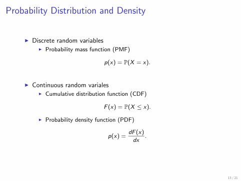
Probability Distribution and Density

I Discrete random variablesI Probability mass function (PMF)

p(x) = P(X = x).

I Continuous random varialesI Cumulative distribution function (CDF)

F (x) = P(X ≤ x).

I Probability density function (PDF)

p(x) =dF (x)

dx.

13 / 21

Gaussian Distribution

Univariate (x ∈ R)

p(x) = N (x |µ, σ2) =1√

2πσ2exp

− 1

2σ2(x − µ)2

.

(a) PDF (b) CDF

[Figure source: Wikipedia]

14 / 21

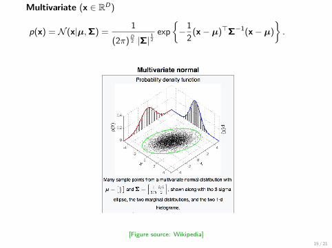
Multivariate (x ∈ RD)

p(x) = N (x|µ,Σ) =1

(2π)D2 |Σ|

12

exp

−1

2(x− µ)>Σ−1(x− µ)

.

[Figure source: Wikipedia]

15 / 21

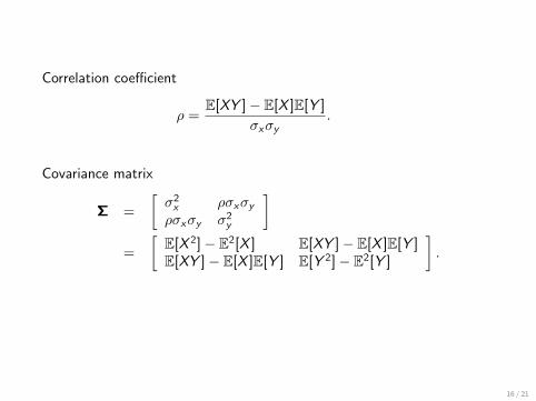
Correlation coefficient

ρ =E[XY ]− E[X ]E[Y ]

σxσy.

Covariance matrix

Σ =

[σ2x ρσxσyρσxσy σ2

y

]=

[E[X 2]− E2[X ] E[XY ]− E[X ]E[Y ]E[XY ]− E[X ]E[Y ] E[Y 2]− E2[Y ]

].

16 / 21

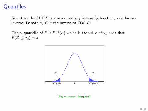
Quantiles

Note that the CDF F is a monotonically increasing function, so it has aninverse. Denote by F−1 the inverse of CDF F .

The α quantile of F is F−1(α) which is the value of xα such thatF (X ≤ xα) = α.

Φ−1(α/2) 0 Φ−1(1−α/2)

α/2 α/2

[Figure source: Murphy’s]

17 / 21

Product and Sum Rules

I Product rule

p(x , y) = p(x |y)p(y).

I Sum rule

p(x) =∑y

p(x , y)

=∑y

p(x |y)p(y).

18 / 21

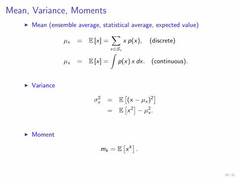
Mean, Variance, Moments

I Mean (ensemble average, statistical average, expected value)

µx = E [x ] =∑x∈Sx

x p(x), (discrete)

µx = E [x ] =

∫p(x) x dx . (continuous).

I Variance

σ2x = E

[(x − µx)2

]= E

[x2]− µ2

x .

I Moment

mk = E[xk].

19 / 21

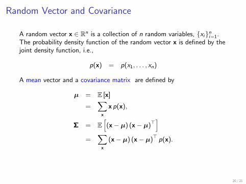
Random Vector and Covariance

A random vector x ∈ Rn is a collection of n random variables, xini=1.The probability density function of the random vector x is defined by thejoint density function, i.e.,

p(x) = p(x1, . . . , xn)

A mean vector and a covariance matrix are defined by

µ = E [x]

=∑

x

x p(x),

Σ = E[(x− µ) (x− µ)>

]=

∑x

(x− µ) (x− µ)> p(x).

20 / 21

Bernoulli & Categorical DistributionsI Bernoulli distribution is the distribution for a single binary random

variable x ∈ 0, 1 parameterized by µ = P(x = 1).

Bern(x |µ) = µx(1− µ)1−x .

I Categorical distribution is a discrete probability distribution thatdescribes the possible results of a random variable that can take onone of K possible elementary events, x ∈ 1, 2, . . . ,K.

p(x) =K∏i=1

P(x = i)I[x=i ].

Or using the 1− of − K encoded random vectors x = [x1, . . . , xK ]>

of dimension K ,

p(x) =K∏i=1

P(x = i)xi .

21 / 21