probability and measurement uncertainty in physic
DESCRIPTION
Probability and Measurement Uncertainty in PhysicTRANSCRIPT

arX
iv:h
ep-p
h/95
1229
5v2
14
Dec
199
5
Probability and Measurement Uncertainty inPhysics
- a Bayesian Primer∗]Notes based on lecturesgiven to graduate students in Rome (May
1995) and summer students at DESY(September 1995).
E-mail: [email protected] file:
http://zow00.desy.de:8000/zeus papers/ZEUS PAPERS/DESY-95-242.ps
-
Giulio D’AgostiniUniversita “La Sapienza” and INFN, Roma, Italy.
Abstract
Bayesian statistics is based on the subjective definition of proba-bility as “degree of belief” and on Bayes’ theorem, the basic tool forassigning probabilities to hypotheses combining a priori judgementsand experimental information. This was the original point of viewof Bayes, Bernoulli, Gauss, Laplace, etc. and contrasts with later“conventional” (pseudo-)definitions of probabilities, which implicitlypresuppose the concept of probability. These notes show that theBayesian approach is the natural one for data analysis in the mostgeneral sense, and for assigning uncertainties to the results of physicalmeasurements - while at the same time resolving philosophical aspects
∗[
1

of the problems. The approach, although little known and usually mis-understood among the High Energy Physics community, has becomethe standard way of reasoning in several fields of research and hasrecently been adopted by the international metrology organizations intheir recommendations for assessing measurement uncertainty.
These notes describe a general model for treating uncertaintiesoriginating from random and systematic errors in a consistent way andinclude examples of applications of the model in High Energy Physics,e.g. “confidence intervals” in different contexts, upper/lower limits,treatment of “systematic errors”, hypothesis tests and unfolding.
2

Contents
3

“The only relevant thing is uncertainty - the extent of ourknowledge and ignorance. The actual fact of whether or not
the events considered are in some sense determined, orknown by other people, and so on, is of no consequence”.
(Bruno de Finetti)
1 Introduction
The purpose of a measurement is to determine the value of a physical quan-tity. One often speaks of the true value, an idealized concept achieved byan infinitely precise and accurate measurement, i.e. immune from errors. Inpractice the result of a measurement is expressed in terms of the best esti-mate of the true value and of a related uncertainty. Traditionally the variouscontributions to the overall uncertainty are classified in terms of “statisti-cal” and “systematic” uncertainties, expressions which reflect the sources ofthe experimental errors (the quote marks indicate that a different way ofclassifying uncertainties will be adopted in this paper).
“Statistical” uncertainties arise from variations in the results of repeatedobservations under (apparently) identical conditions. They vanish if the num-ber of observations becomes very large (“the uncertainty is dominated bysystematics”, is the typical expression used in this case) and can be treated -in most of cases, but with some exceptions of great relevance in High EnergyPhysics - using conventional statistics based on the frequency-based defini-tion of probability.
On the other hand, it is not possible to treat “systematic” uncertaintiescoherently in the frequentistic framework. Several ad hoc prescriptions forhow to combine “statistical” and “systematic” uncertainties can be found intext books and in the literature: “add them linearly”; “add them linearly if. . . , else add them quadratically”; “don’t add them at all”, and so on (see,e.g., part 3 of [1]). The “fashion” at the moment is to add them quadrat-ically if they are considered independent, or to build a covariance matrixof “statistical” and “systematic” uncertainties to treat general cases. Theseprocedures are not justified by conventional statistical theory, but they areaccepted because of the pragmatic good sense of physicists. For example,an experimentalist may be reluctant to add twenty or more contributionslinearly to evaluated the uncertainty of a complicated measurement, or de-cides to treat the correlated “systematic” uncertainties “statistically”, inboth cases unaware of, or simply not caring about, about violating frequen-tistic principles.
4

The only way to deal with these and related problems in a consistent wayis to abandon the frequentistic interpretation of probability introduced atthe beginning of this century, and to recover the intuitive concept of proba-bility as degree of belief. Stated differently, one needs to associate the idea ofprobability to the lack of knowledge, rather than to the outcome of repeatedexperiments. This has been recognized also by the International Organi-zation for Standardization (ISO) which assumes the subjective definition ofprobability in its “Guide to the expression of uncertainty in measurement”[2].
These notes are organized as follow:
• sections 1-5 give a general introduction to subjective probability;
• sections 6-7 summarize some concepts and formulae concerning randomvariables, needed for many applications;
• section 8 introduces the problem of measurement uncertainty and dealswith the terminology.
• sections 9-10 present the analysis model;
• sections 11-13 show several physical applications of the model;
• section 14 deals with the approximate methods needed when the gen-eral solution becomes complicated; in this context the ISO recommen-dations will be presented and discussed;
• section 15 deals with uncertainty propagation. It is particularly shortbecause, in this scheme, there is no difference between the treatmentof “systematic” uncertainties and indirect measurements; the sectionsimply refers the results of sections 11-14;
• section 16 is dedicated to a detailed discussion about the covariancematrix of correlated data and the trouble it may cause;
• section 17 was added as an example of a more complicate inference(multidimensional unfolding) than those treated in sections 11-15.
5

2 Probability
2.1 What is probability?
The standard answers to this question are
1. “the ratio of the number of favorable cases to the number of all cases”;
2. “the ratio of the times the event occurs in a test series to the totalnumber of trials in the series”.
It is very easy to show that neither of these statements can define the conceptof probability:
• Definition (1) lacks the clause “if all the cases are equally probable”.This has been done here intentionally, because people often forget it.The fact that the definition of probability makes use of the term “prob-ability” is clearly embarrassing. Often in text books the clause is re-placed by “if all the cases are equally possible”, ignoring that in thiscontext “possible” is just a synonym of “probable”. There is no wayout. This statement does not define probability but gives, at most, auseful rule for evaluating it - assuming we know what probability is, i.e.of what we are talking about. The fact that this definition is labelled“classical” or “Laplace” simply shows that some authors are not awareof what the “classicals” (Bayes, Gauss, Laplace, Bernoulli, etc) thoughtabout this matter. We shall call this “definition” combinatorial.
• definition (2) is also incomplete, since it lacks the condition that thenumber of trials must be very large (“it goes to infinity”). But this is aminor point. The crucial point is that the statement merely defines therelative frequency with which an event (a “phenomenon”) occurred inthe past. To use frequency as a measurement of probability we have toassume that the phenomenon occurred in the past, and will occur in thefuture, with the same probability. But who can tell if this hypothesisis correct? Nobody: we have to guess in every single case. Notice that,while in the first “definition” the assumption of equal probability wasexplicitly stated, the analogous clause is often missing from the secondone. We shall call this “definition” frequentistic.
We have to conclude that if we want to make use of these statements toassign a numerical value to probability, in those cases in which we judge thatthe clauses are satisfied, we need a better definition of probability.
6

Probability
0,10 0,20 0,30 0,400 0,50 0,60 0,70 0,80 0,90 1
0 1
0
0
E
1
1
?
Event E
logical point of view FALSE
cognitive point of view FALSE
psychological(subjective)
point of view
if certain FALSE
if uncertain,withprobability
UNCERTAIN
TRUE
TRUE
TRUE
Figure 1: Certain and uncertain events.
2.2 Subjective definition of probability
So, “what is probability?” Consulting a good dictionary helps. Webster’sstates, for example, that “probability is the quality, state, or degree of be-ing probable”, and then that probable means “supported by evidence strongenough to make it likely though not certain to be true”. The concept ofprobable arises in reasoning when the concept of certain is not applicable.When it is impossible to state firmly if an event (we use this word as a syn-onym for any possible statement, or proposition, relative to past, present orfuture) is true or false, we just say that this is possible, probable. Differentevents may have different levels of probability, depending whether we thinkthat they are more likely to be true or false (see Fig. 1). The concept ofprobability is then simply
a measure of the degree of belief that an event will1 occur.
This is the kind of definition that one finds in Bayesian books[3, 4, 5, 6, 7]and the formulation cited here is that given in the ISO “Guide to Expressionof Uncertainty in Measurement”[2], of which we will talk later.
At first sight this definition does not seem to be superior to the combi-natorial or the frequentistic ones. At least they give some practical rules tocalculate “something”. Defining probability as “degree of belief” seems too
1The use of the future tense does not imply that this definition can only be applied forfuture events. “Will occur” simply means that the statement “will be proven to be true”,even if it refers to the past. Think for example of “the probability that it was raining inRome on the day of the battle of Waterloo”.
7
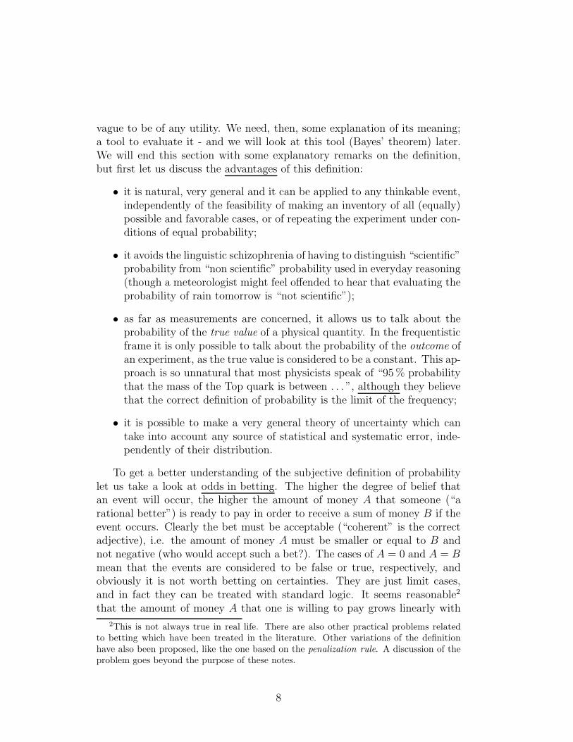
vague to be of any utility. We need, then, some explanation of its meaning;a tool to evaluate it - and we will look at this tool (Bayes’ theorem) later.We will end this section with some explanatory remarks on the definition,but first let us discuss the advantages of this definition:
• it is natural, very general and it can be applied to any thinkable event,independently of the feasibility of making an inventory of all (equally)possible and favorable cases, or of repeating the experiment under con-ditions of equal probability;
• it avoids the linguistic schizophrenia of having to distinguish “scientific”probability from “non scientific” probability used in everyday reasoning(though a meteorologist might feel offended to hear that evaluating theprobability of rain tomorrow is “not scientific”);
• as far as measurements are concerned, it allows us to talk about theprobability of the true value of a physical quantity. In the frequentisticframe it is only possible to talk about the probability of the outcome ofan experiment, as the true value is considered to be a constant. This ap-proach is so unnatural that most physicists speak of “95 % probabilitythat the mass of the Top quark is between . . . ”, although they believethat the correct definition of probability is the limit of the frequency;
• it is possible to make a very general theory of uncertainty which cantake into account any source of statistical and systematic error, inde-pendently of their distribution.
To get a better understanding of the subjective definition of probabilitylet us take a look at odds in betting. The higher the degree of belief thatan event will occur, the higher the amount of money A that someone (“arational better”) is ready to pay in order to receive a sum of money B if theevent occurs. Clearly the bet must be acceptable (“coherent” is the correctadjective), i.e. the amount of money A must be smaller or equal to B andnot negative (who would accept such a bet?). The cases of A = 0 and A = Bmean that the events are considered to be false or true, respectively, andobviously it is not worth betting on certainties. They are just limit cases,and in fact they can be treated with standard logic. It seems reasonable2
that the amount of money A that one is willing to pay grows linearly with
2This is not always true in real life. There are also other practical problems relatedto betting which have been treated in the literature. Other variations of the definitionhave also been proposed, like the one based on the penalization rule. A discussion of theproblem goes beyond the purpose of these notes.
8

the degree of belief. It follows that if someone thinks that the probabilityof the event E is p, then he will bet A = pB to get B if the event occurs,and to lose pB if it does not. It is easy to demonstrate that the condition of“coherence” implies that 0 ≤ p ≤ 1.
What has gambling to do with physics? The definition of probabilitythrough betting odds has to be considered operational, although there isno need to make a bet (with whom?) each time one presents a result. Ithas the important role of forcing one to make an honest assessment of thevalue of probability that one believes. One could replace money with otherforms of gratification or penalization, like the increase or the loss of scientificreputation. Moreover, the fact that this operational procedure is not to betaken literally should not be surprising. Many physical quantities are definedin a similar way. Think, for example, of the text book definition of the electricfield, and try to use it to measure ~E in the proximity of an electron. A niceexample comes from the definition of a poisonous chemical compound: itwould be lethal if ingested. Clearly it is preferable to keep this operationaldefinition at a hypothetical level, even though it is the best definition of theconcept.
2.3 Rules of probability
The subjective definition of probability, together with the condition of co-herence, requires that 0 ≤ p ≤ 1. This is one of the rules which probabilityhas to obey. It is possible, in fact, to demonstrate that coherence yields tothe standard rules of probability, generally known as axioms. At this pointit is worth clarifying the relationship between the axiomatic approach andthe others:
• combinatorial and frequentistic “definitions” give useful rules for eval-uating probability, although they do not, as it is often claimed, definethe concept;
• in the axiomatic approach one refrains from defining what the probabil-ity is and how to evaluate it: probability is just any real number whichsatisfies the axioms. It is easy to demonstrate that the probabilitiesevaluated using the combinatorial and the frequentistic prescriptionsdo in fact satisfy the axioms;
• the subjective approach to probability, together with the coherencerequirement, defines what probability is and provides the rules whichits evaluation must obey; these rules turn out to be the same as theaxioms.
9

C = A BD = A B = A B
c)
A BC
D
h)
E1
E2
Ei
En
F = i=1 (F Ei)n
F
e)
E AC
B
A (B C) = (A B) (A C)D = A B C; E = A B C
D
E E =
E E
a)
A B
b)
A B
C = A B = A B
d)
A BC
C
B
A (B C) = (A B) (A C)
f)
A
E1
E2
Ei
En
n i=1Ei = Ei Ej = O
g)
i,j
Figure 2: Venn diagrams and set properties.
10
Events setssymbol
event set Ecertain event sample space Ωimpossible event empty set ∅implication inclusion E1 ⊆ E2
(subset)opposite event complementary set E (E ∪ E = Ω)(complementary)logical product (“AND”) intersection E1 ∩ E2
logical sum (“OR”) union E1 ∪ E2
incompatible events disjoint sets E1 ∩ E2 = ∅complete class finite partition
Ei ∩ Ej = ∅ (i 6= j)∪iEi = Ω
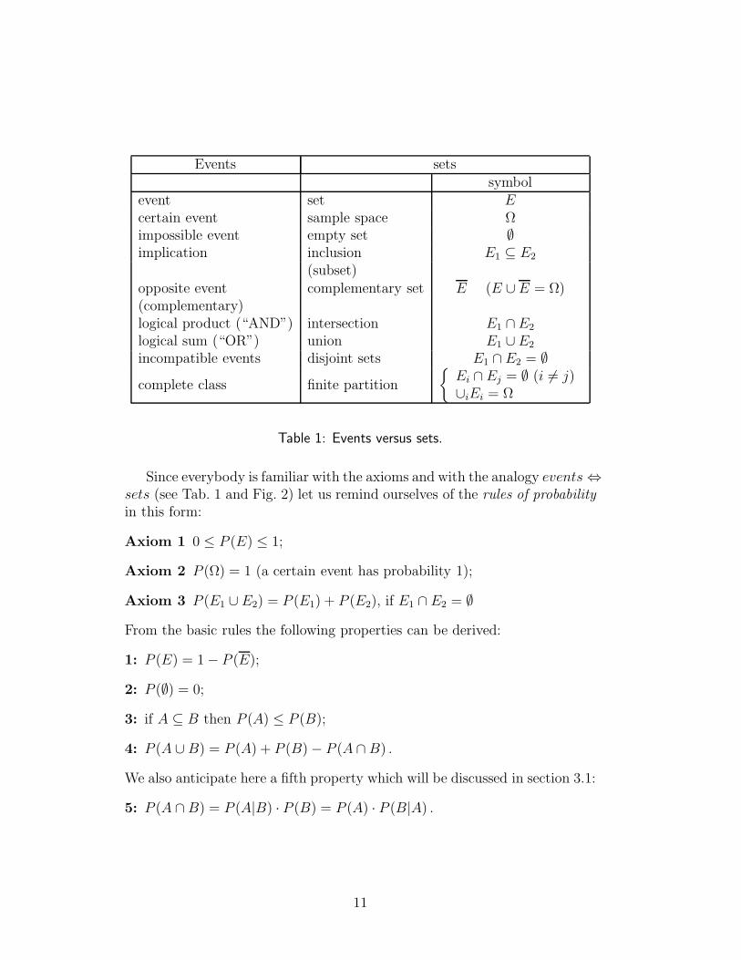
Table 1: Events versus sets.
Since everybody is familiar with the axioms and with the analogy events ⇔sets (see Tab. 1 and Fig. 2) let us remind ourselves of the rules of probabilityin this form:
Axiom 1 0 ≤ P (E) ≤ 1;
Axiom 2 P (Ω) = 1 (a certain event has probability 1);
Axiom 3 P (E1 ∪ E2) = P (E1) + P (E2), if E1 ∩ E2 = ∅
From the basic rules the following properties can be derived:
1: P (E) = 1 − P (E);
2: P (∅) = 0;
3: if A ⊆ B then P (A) ≤ P (B);
4: P (A ∪ B) = P (A) + P (B) − P (A ∩ B) .
We also anticipate here a fifth property which will be discussed in section 3.1:
5: P (A ∩ B) = P (A|B) · P (B) = P (A) · P (B|A) .
11

2.4 Subjective probability and “objective”descriptionof the physical world
The subjective definition of probability seems to contradict the aim of physi-cists to describe the laws of Physics in the most objective way (whateverthis means . . . ). This is one of the reasons why many regard the subjec-tive definition of probability with suspicion (but probably the main reason isbecause we have been taught at University that “probability is frequency”).The main philosophical difference between this concept of probability and anobjective definition that “we would have liked” (but which does not exist inreality) is the fact that P (E) is not an intrinsic characteristic of the eventE, but depends on the status of information available to whoever evaluatesP (E). The ideal concept of “objective” probability is recovered when every-body has the “same” status of information. But even in this case it wouldbe better to speak of intersubjective probability. The best way to convinceourselves about this aspect of probability is to try to ask practical questionsand to evaluate the probability in specific cases, instead of seeking refuge inabstract questions. I find, in fact, that, paraphrasing a famous statementabout Time, “Probability is objective as long as I am not asked to evaluateit”. Some examples:
Example 1: “What is the probability that a molecule of nitrogen at atmo-spheric pressure and room temperature has a velocity between 400 and500 m/s?”. The answer appears easy: “take the Maxwell distributionformula from a text book, calculate an integral and get a number. Nowlet us change the question: “I give you a vessel containing nitrogen anda detector capable of measuring the speed of a single molecule and youset up the apparatus. Now, what is the probability that the first moleculethat hits the detector has a velocity between 400 and 500 m/s?”. Any-body who has minimal experience (direct or indirect) of experimentswould hesitate before answering. He would study the problem carefullyand perform preliminary measurements and checks. Finally he wouldprobably give not just a single number, but a range of possible num-bers compatible with the formulation of the problem. Then he startsthe experiment and eventually, after 10 measurements, he may form adifferent opinion about the outcome of the eleventh measurement.
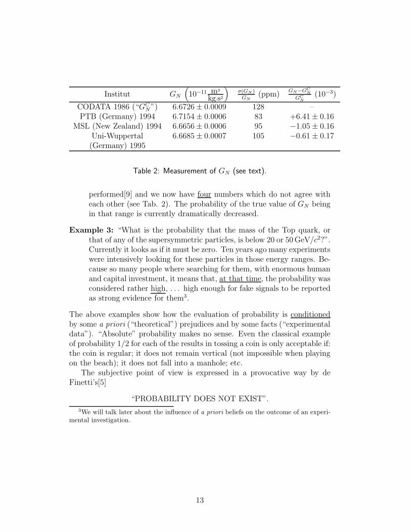
Example 2: “What is the probability that the gravitational constant GN
has a value between 6.6709 · 10−11 and 6.6743 · 10−11 m3kg−1s−2?”.Last year you could have looked at the latest issue of the ParticleData Book[8] and answered that the probability was 95 %. Since then- as you probably know - three new measurements of GN have been
12
Institut GN
(10−11 m3
kg·s2
)σ(GN )
GN(ppm)
GN−GCN
GCN
(10−3)
CODATA 1986 (“GCN”) 6.6726 ± 0.0009 128 –
PTB (Germany) 1994 6.7154 ± 0.0006 83 +6.41 ± 0.16MSL (New Zealand) 1994 6.6656 ± 0.0006 95 −1.05 ± 0.16
Uni-Wuppertal 6.6685 ± 0.0007 105 −0.61 ± 0.17(Germany) 1995
Table 2: Measurement of GN (see text).
performed[9] and we now have four numbers which do not agree witheach other (see Tab. 2). The probability of the true value of GN beingin that range is currently dramatically decreased.
Example 3: “What is the probability that the mass of the Top quark, orthat of any of the supersymmetric particles, is below 20 or 50 GeV/c2?”.Currently it looks as if it must be zero. Ten years ago many experimentswere intensively looking for these particles in those energy ranges. Be-cause so many people where searching for them, with enormous humanand capital investment, it means that, at that time, the probability wasconsidered rather high, . . . high enough for fake signals to be reportedas strong evidence for them3.
The above examples show how the evaluation of probability is conditionedby some a priori (“theoretical”) prejudices and by some facts (“experimentaldata”). “Absolute” probability makes no sense. Even the classical exampleof probability 1/2 for each of the results in tossing a coin is only acceptable if:the coin is regular; it does not remain vertical (not impossible when playingon the beach); it does not fall into a manhole; etc.
The subjective point of view is expressed in a provocative way by deFinetti’s[5]
“PROBABILITY DOES NOT EXIST”.
3We will talk later about the influence of a priori beliefs on the outcome of an experi-mental investigation.
13

3 Conditional probability and Bayes’ theo-
rem
3.1 Dependence of the probability from the status ofinformation
If the status of information changes, the evaluation of the probability also hasto be modified. For example most people would agree that the probabilityof a car being stolen depends on the model, age and parking site. To takean example from physics, the probability that in a HERA detector a chargedparticle of 1 GeV gives a certain number of ADC counts due to the energyloss in a gas detector can be evaluated in a very general way - using HighEnergy Physics jargon - making a (huge) Monte Carlo simulation which takesinto account all possible reactions (weighted with their cross sections), allpossible backgrounds, changing all physical and detector parameters withinreasonable ranges, and also taking into account the trigger efficiency. Theprobability changes if one knows that the particle is a K+: instead of verycomplicated Monte Carlo one can just run a single particle generator. Butthen it changes further if one also knows the exact gas mixture, pressure,. . . , up to the latest determination of the pedestal and the temperature ofthe ADC module.
3.2 Conditional probability
Although everybody knows the formula of conditional probability, it is usefulto derive it here. The notation is P (E|H), to be read “probability of E givenH”, where H stands for hypothesis. This means: the probability that E willoccur if one already knows that H has occurred4.
4P (E|H) should not be confused with P (E ∩ H), “the probability that both eventsoccur”. For example P (E ∩ H) can be very small, but nevertheless P (E|H) very high:think of the limit case
P (H) ≡ P (H ∩ H) ≤ P (H |H) = 1 :
“H given H” is a certain event no matter how small P (H) is, even if P (H) = 0 (in thesense of Section 6.2).
14

The event E|H can have three values:
TRUE: if E is TRUE and H is TRUE;
FALSE: if E is FALSE and H is TRUE;
UNDETERMINED: if H is FALSE; in this case we are merely uninter-ested as to what happens to E. In terms of betting, the bet is invali-dated and none loses or gains.
Then P (E) can be written P (E|Ω), to state explicitly that it is the proba-bility of E whatever happens to the rest of the world (Ω means all possibleevents). We realize immediately that this condition is really too vague andnobody would bet a cent on a such a statement. The reason for usually writ-ing P (E) is that many conditions are implicitly - and reasonably - assumedin most circumstances. In the classical problems of coins and dice, for exam-ple, one assumes that they are regular. In the example of the energy loss, itwas implicit -“obvious”- that the High Voltage was on (at which voltage?)and that HERA was running (under which condition?). But one has to takecare: many riddles are based on the fact that one tries to find a solutionwhich is valid under more strict conditions than those explicitly stated inthe question (e.g. many people make bad business deals signing contracts inwhich what “was obvious” was not explicitly stated).
In order to derive the formula of conditional probability let us assume fora moment that it is reasonable to talk about “absolute probability” P (E) =P (E|Ω), and let us rewrite
P (E) ≡ P (E|Ω) =a
P (E ∩ Ω)
=b
P(E ∩ (H ∪ H)
)
=c
P((E ∩ H) ∪ (E ∩ H)
)
=d
P (E ∩ H) + P (E ∩ H) , (1)
where the result has been achieved through the following steps:
(a): E implies Ω (i.e. E ⊆ Ω) and hence E ∩ Ω = E;
(b): the complementary events H and H make a finite partition of Ω, i.e.H ∪ H = Ω;
(c): distributive property;
(d): axiom 3.
15
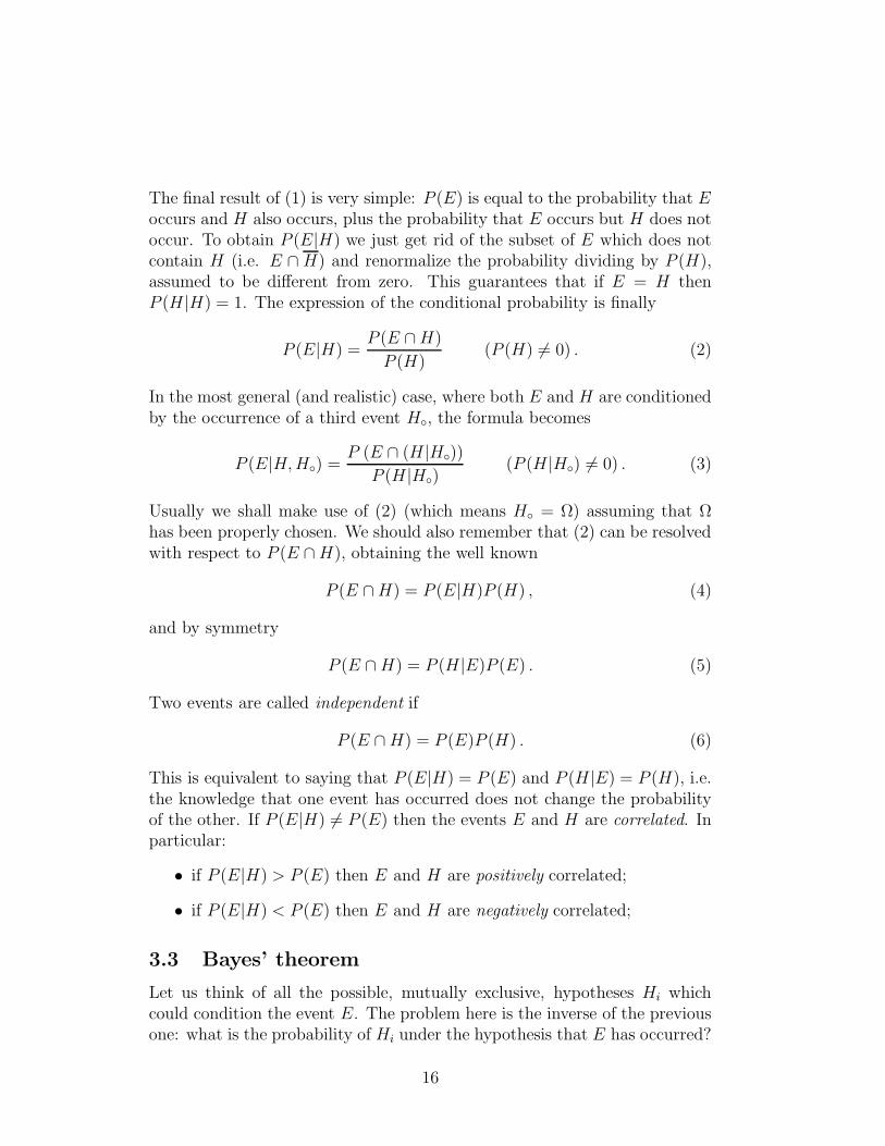
The final result of (1) is very simple: P (E) is equal to the probability that Eoccurs and H also occurs, plus the probability that E occurs but H does notoccur. To obtain P (E|H) we just get rid of the subset of E which does notcontain H (i.e. E ∩ H) and renormalize the probability dividing by P (H),assumed to be different from zero. This guarantees that if E = H thenP (H|H) = 1. The expression of the conditional probability is finally
P (E|H) =P (E ∩ H)
P (H)(P (H) 6= 0) . (2)
In the most general (and realistic) case, where both E and H are conditionedby the occurrence of a third event H, the formula becomes
P (E|H, H) =P (E ∩ (H|H))
P (H|H)(P (H|H) 6= 0) . (3)
Usually we shall make use of (2) (which means H = Ω) assuming that Ωhas been properly chosen. We should also remember that (2) can be resolvedwith respect to P (E ∩ H), obtaining the well known
P (E ∩ H) = P (E|H)P (H) , (4)
and by symmetry
P (E ∩ H) = P (H|E)P (E) . (5)
Two events are called independent if
P (E ∩ H) = P (E)P (H) . (6)
This is equivalent to saying that P (E|H) = P (E) and P (H|E) = P (H), i.e.the knowledge that one event has occurred does not change the probabilityof the other. If P (E|H) 6= P (E) then the events E and H are correlated. Inparticular:
• if P (E|H) > P (E) then E and H are positively correlated;
• if P (E|H) < P (E) then E and H are negatively correlated;
3.3 Bayes’ theorem
Let us think of all the possible, mutually exclusive, hypotheses Hi whichcould condition the event E. The problem here is the inverse of the previousone: what is the probability of Hi under the hypothesis that E has occurred?
16

For example, “what is the probability that a charged particle which went ina certain direction and has lost between 100 and 120 keV in the detector, is aµ, a π, a K, or a p?” Our event E is “energy loss between 100 and 120 keV”,and Hi are the four “particle hypotheses”. This example sketches the basicproblem for any kind of measurement: having observed an effect, to assessthe probability of each of the causes which could have produced it. Thisintellectual process is called inference, and it will be discussed after section 9.
In order to calculate P (Hi|E) let us rewrite the joint probability P (Hi ∩E), making use of (4-5), in two different ways:
P (Hi|E)P (E) = P (E|Hi)P (Hi) , (7)
obtaining
P (Hi|E) =P (E|Hi)P (Hi)
P (E), (8)
or
P (Hi|E)
P (Hi)=
P (E|Hi)
P (E). (9)
Since the hypotheses Hi are mutually exclusive (i.e. Hi ∩Hj = ∅, ∀ i, j) andexhaustive (i.e.
⋃i Hi = Ω), E can be written as E∪Hi, the union of E with
each of the hypotheses Hi. It follows that
P (E) ≡ P (E ∩ Ω) = P
(
E ∩⋃
i
Hi
)
= P
(⋃
i
(E ∩ Hi)
)
=∑
i
P (E ∩ Hi)
=∑
i
P (E|Hi)P (Hi) , (10)
where we have made use of (4) again in the last step. It is then possible torewrite (8) as
P (Hi|E) =P (E|Hi)P (Hi)∑j P (E|Hj)P (Hj)
. (11)
This is the standard form by which Bayes’ theorem is known. (8) and (9) arealso different ways of writing it. As the denominator of (11) is nothing but
17

a normalization factor (such that∑
i P (Hi|E) = 1), the formula (11) can bewritten as
P (Hi|E) ∝ P (E|Hi)P (Hi) . (12)
Factorizing P (Hi) in (11), and explicitly writing the fact that all the eventswere already conditioned by H, we can rewrite the formula as
P (Hi|E, H) = αP (Hi|H) , (13)
with
α =P (E|Hi, H)∑
i P (E|Hi, H)P (Hi|H). (14)
These five ways of rewriting the same formula simply reflect the importancethat we shall give to this simple theorem. They stress different aspects ofthe same concept:
• (11) is the standard way of writing it (although some prefer (8));
• (9) indicates that P (Hi) is altered by the condition E with the sameratio with which P (E) is altered by the condition Hi;
• (12) is the simplest and the most intuitive way to formulate the the-orem: ”the probability of Hi given E is proportional to the initialprobability of Hi times the probability of E given Hi”;
• (13-14) show explicitly how the probability of a certain hypothesis isupdated when the status of information changes:
P (Hi|H) (also indicated as P(Hi)) is the initial, or a priori, proba-
bility (or simply “prior”) of Hi, i.e. the probability of this hypoth-esis with the status of information available before the knowledgethat E has occurred;
P (Hi|E, H) (or simply P (Hi|E)) is the final, or “a posteriori”, prob-
ability of Hi after the new information;
P (E|Hi, H) (or simply P (E|Hi)) is called likelihood.
To better understand the terms “initial”, “final” and “likelihood”, let usformulate the problem in a way closer to the physicist’s mentality, referringto causes and effects: the causes can be all the physical sources which mayproduce a certain observable (the effect). The likelihoods are - as the word
18

says - the likelihoods that the effect follows from each of the causes. Usingour example of the dE/dx measurement again, the causes are all the possi-ble charged particles which can pass through the detector; the effect is theamount of observed ionization; the likelihoods are the probabilities that eachof the particles give that amount of ionization. Notice that in this examplewe have fixed all the other sources of influence: physics process, HERA run-ning conditions, gas mixture, High Voltage, track direction, etc.. This is ourH. The problem immediately gets rather complicated (all real cases, apartfrom tossing coins and dice, are complicated!). The real inference would beof the kind
P (Hi|E, H) ∝ P (E|Hi, H)P (Hi|H)P (H), . (15)
For each status of H (the set of all the possible values of the influenceparameters) one gets a different result for the final probability5. So, insteadof getting a single number for the final probability we have a distribution ofvalues. This spread will result in a large uncertainty of P (Hi|E). This iswhat every physicist knows: if the calibration constants of the detector andthe physics process are not under control, the “systematic errors” are largeand the result is of poor quality.
3.4 Conventional use of Bayes’ theorem
Bayes’ theorem follows directly from the rules of probability, and it can beused in any kind of approach. Let us take an example:
Problem 1: A particle detector has a µ identification efficiency of 95 %, anda probability of identifying a π as a µ of 2 %. If a particle is identifiedas a µ, then a trigger is issued. Knowing that the particle beam is amixture of 90 % π and 10 % µ, what is the probability that a trigger isreally fired by a µ? What is the signal-to-noise (S/N) ratio?
Solution: The two hypotheses (causes) which could condition the event (ef-fect) T (=“trigger fired”) are “µ” and “π”. They are incompatible
5The symbol ∝ could be misunderstood if one forgets that the proportionality factordepends on all likelihoods and priors (see (13)). This means that, for a given hypothesisHi, as the status of information E changes, P (Hi|E, H) may change if P (E|Hi, H)and P (Hi|H) remain constant, if some of the other likelihoods get modified by the newinformation.
19

(clearly) and exhaustive (90%+10%=100%). Then:
P (µ|T ) =P (T |µ)P(µ)
P (T |µ)P(µ) + P (T |π)P(π)(16)
=0.95 × 0.1
0.95 × 0.1 + 0.02 × 0.9= 0.84 ,
and P (π|T ) = 0.16.
The signal to noise ratio is P (µ|T )/P (π|T ) = 5.3. It is interesting torewrite the general expression of the signal to noise ratio if the effectE is observed as
S/N =P (S|E)
P (N |E)=
P (E|S)
P (E|N)· P(S)
P(N). (17)
This formula explicitly shows that when there are noisy conditions
P(S) ≪ P(N)
the experiment must be very selective
P (E|S) ≫ P (E|N)
in order to have a decent S/N ratio.(How does the S/N change if the particle has to be identified by twoindependent detectors in order to give the trigger? Try it yourself, theanswer is S/N = 251.)
Problem 2: Three boxes contain two rings each, but in one of them theyare both gold, in the second both silver, and in the third one of eachtype. You have the choice of randomly extracting a ring from one ofthe boxes, the content of which is unknown to you. You look at theselected ring, and you then have the possibility of extracting a secondring, again from any of the three boxes. Let us assume the first ringyou extract is a gold one. Is it then preferable to extract the secondone from the same or from a different box?
Solution: Choosing the same box you have a 2/3 probability of getting asecond gold ring. (Try to apply the theorem, or help yourself withintuition.)
The difference between the two problems, from the conventional statisticspoint of view, is that the first is only meaningful in the frequentistic ap-proach, the second only in the combinatorial one. They are, however, both
20

acceptable from the Bayesian point of view. This is simply because in thisframework there is no restriction on the definition of probability. In manyand important cases of life and science, neither of the two conventional defi-nitions are applicable.
3.5 Bayesian statistics: learning by experience
The advantage of the Bayesian approach (leaving aside the “little philosoph-ical detail” of trying to define what probability is) is that one may talk aboutthe probability of any kind of event, as already emphasized. Moreover, theprocedure of updating the probability with increasing information is verysimilar to that followed by the mental processes of rational people. Let usconsider a few examples of “Bayesian use” of Bayes’ theorem:
Example 1: Imagine some persons listening to a common friend having aphone conversation with an unknown person Xi, and who are tryingto guess who Xi is. Depending on the knowledge they have about thefriend, on the language spoken, on the tone of voice, on the subject ofconversation, etc., they will attribute some probability to several pos-sible persons. As the conversation goes on they begin to consider somepossible candidates for Xi, discarding others, and eventually fluctuat-ing between two possibilities, until the status of information I is suchthat they are practically sure of the identity of Xi. This experience hashappened to must of us, and it is not difficult to recognize the Bayesianscheme:
P (Xi|I, I) ∝ P (I|Xi, I)P (Xi|I) . (18)
We have put the initial status of information I explicitly in (18) toremind us that likelihoods and initial probabilities depend on it. Ifwe know nothing about the person, the final probabilities will be veryvague, i.e. for many persons Xi the probability will be different fromzero, without necessarily favoring any particular person.
Example 2: A person X meets an old friend F in a pub. F proposes thatthe drinks should be payed for by whichever of the two extracts thecard of lower value from a pack (according to some rule which is of nointerest to us). X accepts and F wins. This situation happens againin the following days and it is always X who has to pay. What is theprobability that F has become a cheat, as the number of consecutivewins n increases?
21

The two hypotheses are: cheat (C) and honest (H). P(C) is low be-cause F is an “old friend”, but certainly not zero (you know . . . ): letus assume 5 %. To make the problem simpler let us make the approxi-mation that a cheat always wins (not very clever. . . ): P (Wn|C) = 1).The probability of winning if he is honest is, instead, given by the rulesof probability assuming that the chance of winning at each trial is 1/2(”why not?”, we shall come back to this point later): P (Wn|H) = 2−n.The result
P (C|Wn) =P (Wn|C) · P(C)
P (Wn|C) · P(C) + P (Wn|H) · P(H)
=1 · P(C)
1 · P(C) + 2−n · P(H)(19)
is shown in the following table:
n P (C|Wn) P (H|Wn)(%) (%)
0 5.0 95.01 9.5 90.52 17.4 82.63 29.4 70.64 45.7 54.35 62.7 37.36 77.1 22.9
. . . . . . . . .
Naturally, as F continues to win the suspicion of X increases. It isimportant to make two remarks:
• the answer is always probabilistic. X can never reach absolutecertainty that F is a cheat, unless he catches F cheating, or Fconfesses to having cheated. This is coherent with the fact thatwe are dealing with random events and with the fact that anysequence of outcomes has the same probability (although there isonly one possibility over 2n in which F is always luckier). Makinguse of P (C|Wn), X can take a decision about the next action totake:
– continue the game, with probability P (C|Wn) of losing, withcertainty, the next time too;
22
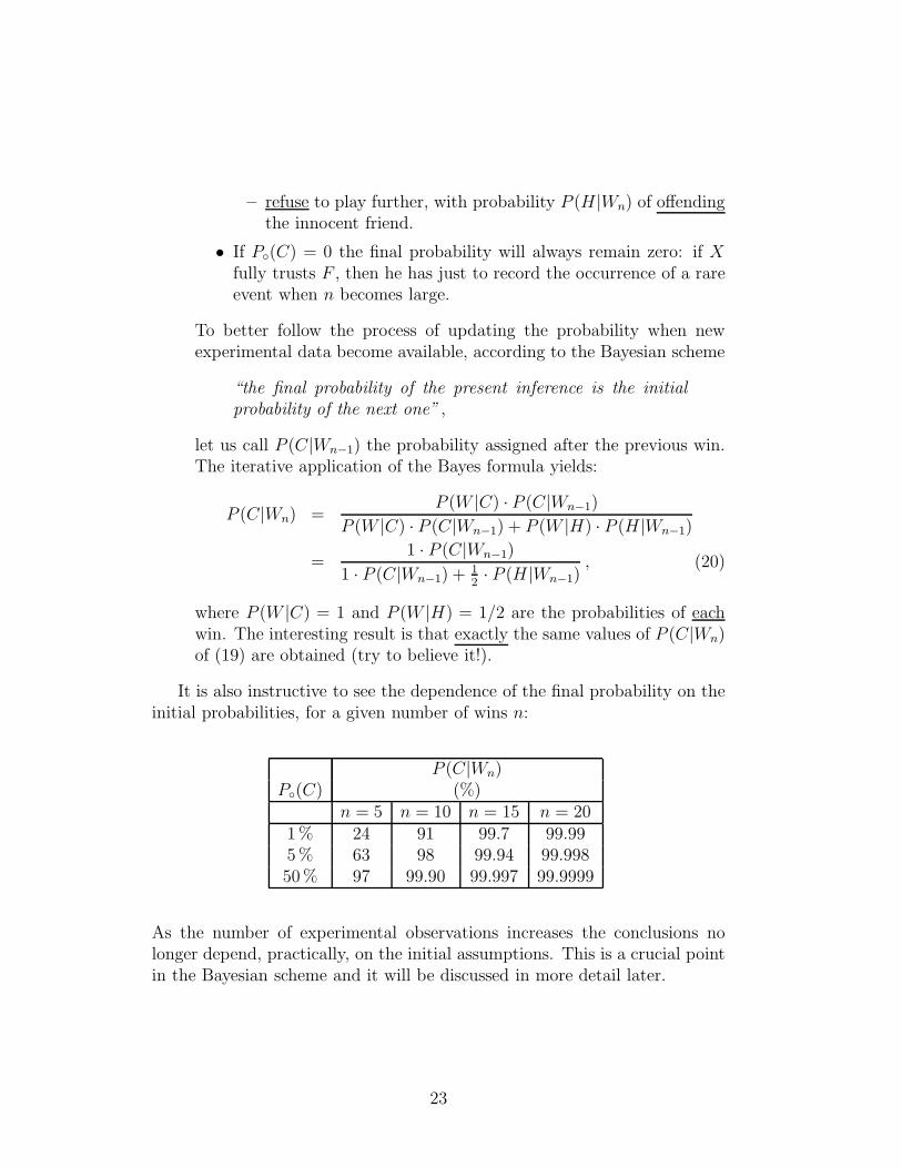
– refuse to play further, with probability P (H|Wn) of offendingthe innocent friend.
• If P(C) = 0 the final probability will always remain zero: if Xfully trusts F , then he has just to record the occurrence of a rareevent when n becomes large.
To better follow the process of updating the probability when newexperimental data become available, according to the Bayesian scheme
“the final probability of the present inference is the initialprobability of the next one” ,
let us call P (C|Wn−1) the probability assigned after the previous win.The iterative application of the Bayes formula yields:
P (C|Wn) =P (W |C) · P (C|Wn−1)
P (W |C) · P (C|Wn−1) + P (W |H) · P (H|Wn−1)
=1 · P (C|Wn−1)
1 · P (C|Wn−1) + 12· P (H|Wn−1)
, (20)
where P (W |C) = 1 and P (W |H) = 1/2 are the probabilities of eachwin. The interesting result is that exactly the same values of P (C|Wn)of (19) are obtained (try to believe it!).
It is also instructive to see the dependence of the final probability on theinitial probabilities, for a given number of wins n:
P (C|Wn)P(C) (%)
n = 5 n = 10 n = 15 n = 201 % 24 91 99.7 99.995 % 63 98 99.94 99.99850 % 97 99.90 99.997 99.9999
As the number of experimental observations increases the conclusions nolonger depend, practically, on the initial assumptions. This is a crucial pointin the Bayesian scheme and it will be discussed in more detail later.
23

4 Hypothesis test (discrete case)
Although in conventional statistics books this argument is usually dealt within one of the later chapters, in the Bayesian approach this is so natural thatit is in fact the first application, as we have seen in the above examples. Wesummarize here the procedure:
• probabilities are attributed to the different hypotheses using initial prob-abilities and experimental data (via the likelihood);
• the person who makes the inference - or the “user” - will take a decisionof which he is fully responsible.
If one needs to compare two hypotheses, as in the example of the signalto noise calculation, the ratio of the final probabilities can be taken as aquantitative result of the test. Let us rewrite the S/N formula in the mostgeneral case:
P (H1|E, H)
P (H2|E, H)=
P (E|H1, H)
P (E|H2, H)· P (H1|H)
P (H2|H), (21)
where again we have reminded ourselves of the existence of H. The ratiodepends on the product of two terms: the ratio of the priors and the ratio ofthe likelihoods. When there is absolutely no reason for choosing between thetwo hypotheses the prior ratio is 1 and the decision depends only on the otherterm, called the Bayes factor. If one firmly believes in either hypothesis, theBayes factor is of minor importance, unless it is zero or infinite (i.e. one andonly one of the likelihoods is vanishing). Perhaps this is disappointing forthose who expected objective certainties from a probability theory, but thisis in the nature of things.
5 Choice of the initial probabilities (discrete
case)
5.1 General criteria
The dependence of Bayesian inferences on initial probability is pointed to byopponents as the fatal flaw in the theory. But this criticism is less severethan one might think at first sight. In fact:
• It is impossible to construct a theory of uncertainty which is not af-fected by this “illness”. Those methods which are advertised as being
24

“objective” tend in reality to hide the hypotheses on which they aregrounded. A typical example is the maximum likelihood method, ofwhich we will talk later.
• as the amount of information increases the dependence on initial prej-udices diminishes;
• when the amount of information is very limited, or completely lacking,there is nothing to be ashamed of if the inference is dominated by apriori assumptions;
The fact that conclusions drawn from an experimental result (and sometimeseven the “result” itself!) often depend on prejudices about the phenomenonunder study is well known to all experienced physicists. Some examples:
• when doing quick checks on a device, a single measurement is usuallyperformed if the value is “what it should be”, but if it is not then manymeasurements tend to be made;
• results are sometimes influenced by previous results or by theoreti-cal predictions. See for example Fig. 3 taken from the Particle DataBook[8]. The interesting book “How experiments end”[10] discusses,among others, the issue of when experimentalists are “happy with theresult” and stop “correcting for the systematics”;
• it can happen that slight deviations from the background are inter-preted as a signal (e.g. as for the first claim of discovery of the Topquark in spring ’94), while larger “signals” are viewed with suspicion ifthey are unwanted by the physics “establishment”6;
• experiments are planned and financed according to the prejudices ofthe moment7;
These comments are not intended to justify unscrupulous behaviour or sloppyanalysis. They are intended, instead, to remind us - if need be - that scien-tific research is ruled by subjectivity much more than outsiders imagine. Thetransition from subjectivity to “objectivity” begins when there is a large con-sensus among the most influential people about how to interpret the results8.
In this context, the subjective approach to statistical inference at leastteaches us that every assumption must be stated clearly and all available in-formation which could influence conclusions must be weighed with the max-imum attempt at objectivity.
6A case, concerning the search for electron compositeness in e+e− collisions, is discussed
25

1950 1960 1970 1980 1990 2000
neut
ron
lifet
ime
(s)
1200
1150
1100
1050
1000
950
900
850
1950 1960 1970 1980 1990 2000
KS m
ean
lifet
ime
(ps)
0
105
85
80
100
95
90
Figure 3: Results on two physical quantities as a function of the publication date.
26

Figure 4: R = σL/σT as a function of the Deep Inelastic Scattering variable xas measured by experiments and as predicted by QCD.
27

What are the rules for choosing the “right” initial probabilities? As onecan imagine, this is an open and debated question among scientists andphilosophers. My personal point of view is that one should avoid pedanticdiscussion of the matter, because the idea of universally true priors remindsme terribly of the famous “angels’ sex” debates.
If I had to give recommendations, they would be:
• the a priori probability should be chosen in the same spirit as therational person who places a bet, seeking to minimize the risk of losing;
• general principles - like those that we will discuss in a while - mayhelp, but since it may be difficult to apply elegant theoretical ideas inall practical situations, in many circumstances the guess of the “expert”can be relied on for guidance.
• avoid using as prior the results of other experiments dealing with thesame open problem, otherwise correlations between the results wouldprevent all comparison between the experiments and thus the detectionof any systematic errors. I find that this point is generally overlookedby statisticians.
5.2 Insufficient Reason and Maximum Entropy
The first and most famous criterion for choosing initial probabilities is thesimple Principle of Insufficient Reason (or Indifference Principle): if thereis no reason to prefer one hypothesis over alternatives, simply attribute thesame probability to all of them. This was stated as a principle by Laplace9
in contrast to Leibnitz’ famous Principle of Sufficient Reason, which, in sim-ple words, states that ”nothing happens without a reason”. The indifferenceprinciple applied to coin and die tossing, to card games or to other simple andsymmetric problems, yields to the well known rule of probability evaluationthat we have called combinatorial. Since it is impossible not to agree with
in [11].7For a recent delightful report, see [12].8“A theory needs to be confirmed by experiments. But it is also true that an experi-
mental result needs to be confirmed by a theory”. This sentence expresses clearly - thoughparadoxically - the idea that it is difficult to accept a result which is not rationally jus-tified. An example of results “not confirmed by the theory” are the R measurements inDeep Inelastic Scattering shown in Fig. 4. Given the conflict in this situation, physiciststend to believe more in QCD and use the “low-x” extrapolations (of what?) to correct thedata for the unknown values of R.
9It may help in understanding Laplace’s approach if we consider that he called thetheory of probability “good sense turned into calculation”.
28
this point of view, in the cases that one judges that it does apply, the com-binatorial “definition” of probability is recovered in the Bayesian approachif the word “definition” is simply replaced by “evaluation rule”. We have infact already used this reasoning in previous examples.
A modern and more sophisticated version of the Indifference Principleis the Maximum Entropy Principle. The information entropy function of nmutually exclusive events, to each of which a probability pi is assigned, isdefined as
H(p1, p2, . . . pn) = −K
n∑
i=1
pi ln pi, (22)
with K a positive constant. The principle states that “in making inferenceson the basis of partial information we must use that probability distribu-tion which has the maximum entropy subject to whatever is known[13]”.Notice that, in this case, “entropy” is synonymous with “uncertainty”[13].One can show that, in the case of absolute ignorance about the events Ei,the maximization of the information uncertainty, with the constraint that∑n
i=1 pi = 1, yields the classical pi = 1/n (any other result would have beenworrying. . . ).
Although this principle is sometimes used in combination with the Bayes’formula for inferences (also applied to measurement uncertainty, see [14]), itwill not be used for applications in these notes.
6 Random variables
In the discussion which follows I will assume that the reader is familiar withrandom variables, distributions, probability density functions, expected val-ues, as well as with the most frequently used distributions. This section isonly intended as a summary of concepts and as a presentation of the notationused in the subsequent sections.
6.1 Discrete variables
Stated simply, to define a random variable X means to find a rule whichallows a real number to be related univocally (but not biunivocally) to anevent (E), chosen from those events which constitute a finite partition ofΩ (i.e. the events must be exhaustive and mutually exclusive). One couldwrite this expression X(E). If the number of possible events is finite thenthe random variable is discrete, i.e. it can assume only a finite number ofvalues. Since the chosen set of events are mutually exclusive, the probability
29

of X = x is the sum of the probabilities of all the events for which X(Ei) = x.Note that we shall indicate the variable with X and its numerical realizationwith x, and that, differently from other notations, the symbol x (in place ofn or k) is also used for discrete variables.
After this short introduction, here is a list of definitions, properties andnotations:
Probability function:
f(x) = P (X = x) . (23)
It has the following properties:
1) 0 ≤ f(xi) ≤ 1 ; (24)
2) P (X = xi ∪ X = xj) = f(xi) + f(xj) ; (25)
3)∑
i
f(xi) = 1 . (26)
Cumulative distribution function:
F (xk) ≡ P (X ≤ xk) =∑
xi≤xk
f(xi) . (27)
Properties:
1) F (−∞) = 0 (28)
2) F (+∞) = 1 (29)
3) F (xi) − F (xi−1) = f(xi) (30)
4) limǫ→o
F (x + ǫ) = F (x) (right side continuity) . (31)
Expected value (mean):
µ ≡ E[X] =∑
i
xif(xi) . (32)
In general, given a function g(X) of X:
E[g(X)] =∑
i
g(xi)f(xi) . (33)
E[·] is a linear operator:
E[aX + b] = aE[X] + b . (34)
30

Variance and standard deviation: Variance:
σ2 ≡ V ar(X) = E[(X − µ)2] = E[X2] − µ2 . (35)
Standard deviation:
σ = +√
σ2 . (36)
Transformation properties:
V ar(aX + b) = a2V ar(X) ; (37)
σ(aX + b) = |a|σ(X) . (38)
Binomial distribution: X ∼ Bn,p (hereafter “∼” stands for “follows”);Bn,p stands for binomial with parameters n (integer) and p (real):
f(x|Bn,p) =n!
(n − x)!x!px(1 − p)n−x ,
n = 1, 2, . . . ,∞0 ≤ p ≤ 1x = 0, 1, . . . , n
.(39)
Expected value, standard deviation and variation coefficient:
µ = np (40)
σ =√
np(1 − p) (41)
v ≡ σ
µ=
√np(1 − p)
np∝ 1√
n. (42)
1 − p is often indicated by q.
Poisson distribution: X ∼ Pλ:
f(x|Pλ) =λx
x!e−λ
0 < λ < ∞x = 0, 1, . . . ,∞ . (43)
(x is integer, λ is real.)Expected value, standard deviation and variation coefficient:
µ = λ (44)
σ =√
λ (45)
v =1√λ
(46)
Binomial → Poisson:
Bn,p −−−−−−−−→n → “∞′′
p → “0′′
(λ = np)
Pλ . (47)
31

6.2 Continuous variables: probability and density func-tion
Moving from discrete to continuous variables there are the usual problemswith infinite possibilities, similar to those found in Zeno’s “Achilles and thetortoise” paradox. In both cases the answer is given by infinitesimal calculus.But some comments are needed:
• the probability of each of the realizations of X is zero (P (X = x) = 0),but this does not mean that each value is impossible, otherwise it wouldbe impossible to get any result;
• although all values x have zero probability, one usually assigns differ-ent degrees of belief to them, quantified by the probability densityfunction f(x). Writing f(x1) > f(x2), for example, indicates that ourdegree of belief in x1 is greater than that in x2.
• The probability that a random variable lies inside a finite interval, forexample P (a ≤ X ≤ b), is instead finite. If the distance between aand b becomes infinitesimal, then the probability becomes infinitesimaltoo. If all the values of X have the same degree of belief (and not onlyequal numerical probability P (x) = 0) the infinitesimal probability issimply proportional to the infinitesimal interval dP = kdx. In thegeneral case the ratio between two infinitesimal probabilities aroundtwo different points will be equal to the ratio of the degrees of belief inthe points (this argument implies the continuity of f(x) on either sideof the values). It follows that dP = f(x)dx and then
P (a ≤ X ≤ b) =
∫ b
a
f(x)dx ; (48)
• f(x) has a dimension inverse to that of the random variable.
After this short introduction, here is a list of definitions, properties andnotations:
Cumulative distribution function:
F (x) = P (X ≤ x) =
∫ x
−∞f(x′)dx′ , (49)
or
f(x) =dF (x)
dx(50)
32

Properties of f(x) and F (x):
• f(x) ≥ 0 ;
•∫ +∞−∞ f(x)dx = 1 ;
• 0 ≤ F (x) ≤ 1;
• P (a ≤ X ≤ b) =∫ b
af(x)dx =
∫ b
−∞ f(x)dx −∫ a
−∞ f(x)dx= F (b) − F (a);
• if x2 > x1 then F (x2) ≥ F (x1) .
• limx→−∞ F (x) = 0 ;limx→+∞ F (x) = 1 ;
Expected value:
E[X] =
∫ +∞
−∞xf(x)dx (51)
E[g(X)] =
∫ +∞
−∞g(x)f(x)dx. (52)
Uniform distribution: 10 X ∼ K(a, b):
f(x|K(a, b)) =1
b − a(a ≤ x ≤ b) (53)
F (x|K(a, b)) =x − a
b − a. (54)
Expected value and standard deviation:
µ =a + b
2(55)
σ =b − a√
12. (56)
Normal (gaussian) distribution: X ∼ N (µ, σ):
f(x|N (µ, σ)) =1√2πσ
e−(x−µ)2
2σ2
−∞ < µ < +∞0 < σ < ∞−∞ < x < +∞
,(57)
where µ and σ (both real) are the expected value and standard devia-tion, respectively.
10The symbols of the following distributions have the parameters within parentheses toindicate that the variables are continuous.
33

Standard normal distribution: the particular normal distribution of mean0 and standard deviation 1, usually indicated by Z:
Z ∼ N (0, 1) . (58)
Exponential distribution: T ∼ E(τ):
f(t|E(τ)) =1
τe−t/τ
0 ≤ τ < ∞0 ≤ t < ∞ (59)
F (t|E(τ)) = 1 − e−t/τ (60)
we use of the symbol t instead of x because this distribution will beapplied to the time domain.Survival probability:
P (T > t) = 1 − F (t|E(τ)) = e−t/τ (61)
Expected value and standard deviation:
µ = τ (62)
σ = τ. (63)
The real parameter τ has the physical meaning of lifetime.
Poisson ↔ Exponential: If X (= “number of counts during the time ∆t”)is Poisson distributed then T (=“interval of time to be waited - startingfrom any instant - before the first count is recorded”) is exponentiallydistributed:
X ∼ f(x|Pλ) ⇐⇒ T ∼ f(x|E(τ)) (64)
(τ = ∆Tλ
) (65)
6.3 Distribution of several random variables
We only consider the case of two continuous variables (X and Y ). Theextension to more variables is straightforward. The infinitesimal element ofprobability is dF (x, y) = f(x, y)dxdy, and the probability density function
f(x, y) =∂2F (x, y)
∂x∂y. (66)
The probability of finding the variable inside a certain area A is∫∫
A
f(x, y)dxdy . (67)
34

Marginal distributions:
fX(x) =
∫ +∞
−∞f(x, y)dy (68)
fY (y) =
∫ +∞
−∞f(x, y)dx . (69)
The subscripts X and Y indicate that fX(x) and fY (y) are only functionof X and Y , respectively (to avoid fooling around with different symbolsto indicate the generic function).
Conditional distributions:
fX(x|y) =f(x, y)
fY (y)=
f(x, y)∫f(x, y)dx
(70)
fY (y|x) =f(x, y)
fX(x)(71)
f(x, y) = fX(x|y)fY (y) (72)
= fY (y|x)fY (x) . (73)
Independent random variables
f(x, y) = fX(x)fY (y) (74)
(it implies f(x|y) = fX(x) and f(y|x) = fY (y) .)
Bayes’ theorem for continuous random variables
f(h|e) =f(e|h)fh(h)∫f(e|h)fh(h)dh
. (75)
Expected value:
µX = E[X] =
∫ ∫ +∞
−∞xf(x, y)dxdy (76)
=
∫ +∞
−∞xfX(x)dx , (77)
and analogously for Y . In general
E[g(X, Y )] =
∫ ∫ +∞
−∞g(x, y)f(x, y)dxdy . (78)
35

Variance:
σ2X = E[X2] − E2[X] , (79)
and analogously for Y .
Covariance:
Cov(X, Y ) = E [(X − E[X]) (Y − E[Y ])] (80)
= E[XY ] − E[X]E[Y ] . (81)
If Y and Y are independent, then E[XY ] = E[X]E[Y ] and henceCov(X, Y ) = 0 (the opposite is true only if X, Y ∼ N (·)).
Correlation coefficient:
ρ(X, Y ) =Cov(X, Y )√
V ar(X)V ar(Y )(82)
=Cov(X, Y )
σXσY. (83)
(−1 ≤ ρ ≤ 1)
Linear combinations of random variables:If Y =
∑i ciXi, with ci real, then:
µY = E[Y ] =∑
i
ciE[Xi] =∑
i
ciµi (84)
σ2Y = V ar(Y ) =
∑
i
c2i V ar(Xi) + 2
∑
i<j
cicjCov(Xi, Xj) (85)
=∑
i
c2i V ar(Xi) +
∑
i6=j
cicjCov(Xi, Xj) (86)
=∑
i
c2i σ
2i +
∑
i6=j
ρijcicjσiσj (87)
=∑
ij
ρijcicjσiσj (88)
=∑
ij
cicjσij . (89)
σ2Y has been written in the different ways, with increasing levels of
compactness, that can be found in the literature. In particular, (89)uses the convention σii = σ2
i and the fact that, by definition, ρii = 1.
36

Figure 5: Example of bivariate normal distribution.
37

Bivariate normal distribution: joint probability density function of Xand Y with correlation coefficient ρ (see Fig 5):
f(x, y) =1
2πσxσy
√1 − ρ2
· (90)
exp
− 1
2(1 − ρ2)
[(x − µx)
2
σ2x
− 2ρ(x − µx)(y − µy)
σxσy
+(y − µy)
2
σ2y
].
Marginal distributions:
X ∼ N (µx, σx) (91)
Y ∼ N (µy, σy) . (92)
Conditional distribution:
f(y|x) =1√
2πσy
√1 − ρ2
exp
−
(y −
[µy + ρσy
σx(x − µx)
])2
2σ2y(1 − ρ2)
,(93)
i.e.
Y|x∼ N
(µy + ρ
σy
σx
(x − µx) , σy
√1 − ρ2
): (94)
the condition X = x squeezes the standard deviation and shifts themean of Y .
7 Central limit theorem
7.1 Terms and role
The well known central limit theorem plays a crucial role in statistics andjustifies the enormous importance that the normal distribution has in manypractical applications (this is the reason why it appears on 10 DM notes).
We have reminded ourselves in (84-85) of the expression of the mean andvariance of a linear combination of random variables
Y =
n∑
i=1
Xi
in the most general case, which includes correlated variables (ρij 6= 0). Inthe case of independent variables the variance is given by the simpler, andbetter known, expression
σ2Y =
n∑
i=1
c2i σ
2i (ρij = 0, i 6= j) . (95)
38

Figure 6: Central limit theorem at work: the sum of n variables, for two differentdistribution, is shown. The values of n (top-down) are: 1,2,3,5,10,20,50.
39

This is a very general statement, valid for any number and kind of variables(with the obvious clause that all σi must be finite) but it does not give anyinformation about the probability distribution of Y . Even if all Xi follow thesame distributions f(x), f(y) is different from f(x), with some exceptions,one of these being the normal.
The central limit theorem states that the distribution of a linear combi-nation Y will be approximately normal if the variables Xi are independentand σ2
Y is much larger than any single component c2i σ
2i from a non-normally
distributed Xi. The last condition is just to guarantee that there is no sin-gle random variable which dominates the fluctuations. The accuracy of theapproximation improves as the number of variables n increases (the theoremsays “when n → ∞”):
n → ∞ =⇒ Y ∼ N
n∑
i=1
ciXi,
(n∑
i=1
c2i σ
2i
)12
(96)
The proof of the theorem can be found in standard text books. For practicalpurposes, and if one is not very interested in the detailed behavior of thetails, n equal to 2 or 3 may already gives a satisfactory approximation, es-pecially if the Xi exhibits a gaussian-like shape. Look for example at Fig. 6,where samples of 10000 events have been simulated starting from a uniformdistribution and from a crazy square wave distribution. The latter, depictinga kind of “worst practical case”, shows that, already for n = 20 the distribu-tion of the sum is practically normal. In the case of the uniform distributionn = 3 already gives an acceptable approximation as far as probability inter-vals of one or two standard deviations from the mean value are concerned.The figure also shows that, starting from a triangular distribution (obtainedin the example from the sum of 2 uniform distributed variables), n = 2 isalready sufficient (the sum of 2 triangular distributed variables is equivalentto the sum of 4 uniform distributed variables).
7.2 Distribution of a sample average
As first application of the theorem let us remind ourselves that a sampleaverage Xnof n independent variables
Xn =
n∑
i=1
1
nXi, (97)
40

is normally distributed, since it is a linear combination of n variables Xi,with ci = 1/n. Then:
Xn ∼ N (µXn, σXn
) (98)
µXn=
n∑
i=1
1
nµ = µ (99)
σ2Xn
=n∑
i=1
(1
n
)2
σ2 =σ2
n(100)
σXn=
σ√n
. (101)
This result, we repeat, is independent of the distribution of X and is alreadyapproximately valid for small values of n.
7.3 Normal approximation of the binomial and of thePoisson distribution
Another important application of the theorem is that the binomial and thePoisson distribution can be approximated, for “large numbers”, by a normaldistribution. This is a general result, valid for all distributions which havethe reproductive property under the sum. Distributions of this kind are thebinomial, the Poisson and the χ2. Let us go into more detail:
Bn,p → N(np,√
np(1 − p))
The reproductive property of the binomial states
that if X1, X2, . . . , Xm are m independent variables, each following abinomial distribution of parameter ni and p, then their sum Y =
∑i Xi
also follows a binomial distribution with parameters n =∑
i ni and p.It is easy to be convinced of this property without any mathematics:just think of what happens if one tosses bunches of three, of five andof ten coins, and then one considers the global result: a binomial witha large n can then always be seen as a sum of many binomials withsmaller ni. The application of the central limit theorem is straight-forward, apart from deciding when the convergence is acceptable: theparameters on which one has to judge are in this case µ = np and thecomplementary quantity µc = n(1− p) = n − µ. If they are both & 10then the approximation starts to be reasonable.
Pλ → N(λ,
√λ)
The same argument holds for the Poisson distribution. In
this case the approximation starts to be reasonable when µ = λ & 10.
41
7.4 Normal distribution of measurement errors
The central limit theorem is also important to justify why in many casesthe distribution followed by the measured values around their average isapproximately normal. Often, in fact, the random experimental error e,which causes the fluctuations of the measured values around the unknowntrue value of the physical quantity, can be seen as an incoherent sum ofsmaller contributions
e =∑
i
ei , (102)
each contribution having a distribution which satisfies the conditions of thecentral limit theorem.
7.5 Caution
After this commercial in favour of the miraculous properties of the centrallimit theorem, two remarks of caution:
• sometimes the conditions of the theorem are not satisfied:
– a single component dominates the fluctuation of the sum: a typicalcase is the well known Landau distribution; also systematic errorsmay have the same effect on the global error;
– the condition of independence is lost if systematic errors affect aset of measurements, or if there is coherent noise;
• the tails of the distributions do exist and they are not always gaussian!Moreover, realizations of a random variable several standard deviationsaway from the mean are possible. And they show up without notice!
8 Measurement errors and measurement un-
certainty
One might assume that the concepts of error and uncertainty are well enoughknown to be not worth discussing. Nevertheless a few comments are needed(although for more details to the DIN[1] and ISO[2, 15] recommendationsshould be consulted):
• the first concerns the terminology. In fact the words error and uncer-tainty are currently used almost as synonyms:
42

– “error” to mean both error and uncertainty (but nobody says“Heisenberg Error Principle”);
– “uncertainty” only for the uncertainty.
“Usually” we understand what each other is talking about, but a moreprecise use of these nouns would really help. This is strongly calledfor by the DIN[1] and ISO[2, 15] recommendations. They state in factthat
– error is “the result of a measurement minus a true value of themeasurand”: it follows that the error is usually unkown;
– uncertainty is a “parameter, associated with the result of a mea-surement, that characterizes the dispersion of the values that couldreasonably be attributed to the measurand”;
• Within the High Energy Physics community there is an establishedpractice for reporting the final uncertainty of a measurement in theform of standard deviation. This is also recommended by these norms.However this should be done at each step of the analysis, instead ofestimating “maximum error bounds” and using them as standard de-viation in the “error propagation”;
• the process of measurement is a complex one and it is difficult to dis-entangle the different contributions which cause the total error. Inparticular, the active role of the experimentalist is sometimes over-looked. For this reason it is often incorrect to quote the (“nominal”)uncertainty due to the instrument as if it were the uncertainty of themeasurement.
9 Statistical Inference
9.1 Bayesian inference
In the Bayesian framework the inference is performed calculating the finaldistribution of the random variable associated to the true values of the physi-cal quantities from all available information. Let us call x = x1, x2, . . . , xnthe n-tuple (“vector”) of observables, µ = µ1, µ2, . . . , µn the n-tuple of thetrue values of the physical quantities of interest, and h = h1, h2, . . . , hnthe n-tuple of all the possible realizations of the influence variables Hi. Theterm “influence variable” is used here with an extended meaning, to indi-cate not only external factors which could influence the result (temperature,
43

atmospheric pressure, and so on) but also any possible calibration constantand any source of systematic errors. In fact the distinction between µ andh is artificial, since they are all conditional hypotheses. We separate themsimply because at the end we will “marginalize” the final joint distributionfunctions with respect to µ, integrating the joint distribution with respect tothe other hypotheses considered as influence variables.
The likelihood of the sample x being produced from h and µ and theinitial probability are
f(x|µ, h, H)
and
f(µ, h) = f(µ, h|H) , (103)
respectively. H is intended to remind us, yet again, that likelihoods and pri-ors - and hence conclusions - depend on all explicit and implicit assumptionswithin the problem, and in particular on the parametric functions used tomodel priors and likelihoods. To simplify the formulae, H will no longer bewritten explicitly.
Using the Bayes formula for multidimensional continuous distributions(an extension of ( 75)) we obtain the most general formula of inference
f(µ, h|x) =f(x|µ, h)f(µ, h)∫
f(x|µ, h)f(µ, h)dµdh, (104)
yielding the joint distribution of all conditional variables µ and h which areresponsible for the observed sample x. To obtain the final distribution of µone has to integrate (104) over all possible values of h, obtaining
f(µ|x) =
∫f(x|µ, h)f(µ, h)dh∫
f(x|µ, h)f(µ, h)dµdh. (105)
Apart from the technical problem of evaluating the integrals, if need be nu-merically or using Monte Carlo methods11, (105) represents the most generalform of hypothetical inductive inference. The word “hypothetical” remindsus of H.
When all the sources of influence are under control, i.e. they can beassumed to take a precise value, the initial distribution can be factorized by
11This is conceptually what experimentalists do when they change all the parameters ofthe Monte Carlo simulation in order to estimate the “systematic error”.
44

a f(µ) and a Dirac δ(h − h), obtaining the much simpler formula
f(µ|x) =
∫f(x|µ, h)f(µ)δ(h − h)dh∫
f(x|µ, h)f(µ)δ(h − h)dµdh
=f(x|µ, h)f(µ)∫f(x|µ, h)f(µ)dµ
. (106)
Even if formulae (105-106) look complicated because of the multidimensionalintegration and of the continuous nature of µ, conceptually they are identicalto the example of the dE/dx measurement discussed in Sec. 9.1
The final probability density function provides the most complete anddetailed information about the unknown quantities, but sometimes (almostalways . . . ) one is not interested in full knowledge of f(µ), but just in afew numbers which summarize at best the position and the width of thedistribution (for example when publishing the result in a journal in the mostcompact way). The most natural quantities for this purpose are the expectedvalue and the variance, or the standard deviation. Then the Bayesian bestestimate of a physical quantity is:
µi = E[µi] =
∫µif(µ|x)dµ (107)
σ2µi
≡ V ar(µi) = E[µ2i ] − E2[µi] (108)
σµi≡ +
√σ2
µi(109)
When many true values are inferred from the same data the numberswhich synthesize the result are not only the expected values and variances,but also the covariances, which give at least the (linear!) correlation coeffi-cients between the variables:
ρij ≡ ρ(µi, µj) =Cov(µi, µj)
σµiσµj
. (110)
In the following sections we will deal in most cases with only one value toinfer:
f(µ|x) = . . . , (111)
9.2 Bayesian inference and maximum likelihood
We have already said that the dependence of the final probabilities on theinitial ones gets weaker as the amount of experimental information increases.
45

Without going into mathematical complications (the proof of this statementcan be found for example in[3]) this simply means that, asymptotically, what-ever f(µ) one puts in (106), f(µ|x) is unaffected. This is “equivalent” todropping f(µ) from (106). This results in
f(µ|x) ≈ f(x|µ, h)∫f(x|µ, h)dµ
. (112)
Since the denominator of the Bayes formula has the technical role of properlynormalizing the probability density function, the result can be written in thesimple form
f(µ|x) ∝ f(x|µ, h) ≡ L(x; µ, h) . (113)
Asymptotically the final probability is just the (normalized) likelihood! Thenotation L is that used in the maximum likelihood literature (note that, notonly does f become L, but also “|” has been replaced by “;”: L has noprobabilistic interpretation in conventional statistics.)
If the mean value of f(µ|x) coincides with the value for which f(µ|x) hasa maximum, we obtain the maximum likelihood method. This does not meanthat the Bayesian methods are “blessed” because of this achievement, andthat they can be used only in those cases where they provide the same results.It is the other way round, the maximum likelihood method gets justified whenall the the limiting conditions of the approach (→ insensitivity of the resultfrom the initial probability → large number of events) are satisfied.
Even if in this asymptotic limit the two approaches yield the same nu-merical results, there are differences in their interpretation:
• the likelihood, after proper normalization, has a probabilistic meaningfor Bayesians but not for frequentists; so Bayesians can say that theprobability that µ is in a certain interval is, for example, 68 %, whilethis statement is blasphemous for a frequentist (“the true value is aconstant” from his point of view);
• frequentists prefer to choose µL the value which maximizes the likeli-hood, as estimator. For Bayesians, on the other hand, the expectedvalue µB = E[µ] (also called the prevision) is more appropriate. Thisis justified by the fact that the assumption of the E[µ] as best estimateof µ minimizes the risk of a bet (always keep the bet in mind!). For ex-ample, if the final distribution is exponential with parameter τ (let usthink for a moment of particle decays) the maximum likelihood methodwould recommend betting on the value t = 0, whereas the Bayesian ap-proach suggests the value t = τ . If the terms of the bet are “whoever
46

gets closest wins” what is the best strategy? And then, what is thebest strategy if the terms are “whoever gets the exact value wins”?But now think of the probability of getting the exact value and of theprobability of getting closest?
9.3 The dog, the hunter and the biased Bayesian esti-mators
One of the most important tests to judge how good an estimator is, is whetheror not it is correct (not biased). Maximum likelihood estimators are usuallycorrect, while Bayesian estimators - analysed within the maximum likelihoodframework - often are not. This could be considered a weak point - howeverthe Bayes estimators are simply naturally consistent with the status of in-formation before new data become available. In the maximum likelihoodmethod, on the other hand, it is not clear what the assumptions are.
Let us take an example which shows the logic of frequentistic inferenceand why the use of reasonable prior distributions yields results which thatframe classifies as distorted. Imagine meeting a hunting dog in the country.Let us assume we know that there is a 50 % probability of finding the dogwithin a radius of 100 meters centered on the position of the hunter (this isour likelihood). Where is the hunter? He is with 50 % probability within aradius of 100 meters around the position of the dog, with equal probabilityin all directions. “Obvious”. This is exactly the logic scheme used in thefrequentistic approach to build confidence regions from the estimator (thedog in this example). This however assumes that the hunter can be anywherein the country. But now let us change the status of information: “the dog isby a river”; “the dog has collected a duck and runs in a certain direction”;“the dog is sleeping”; “the dog is in a field surrounded by a fence throughwhich he can pass without problems, but the hunter cannot”. Given anynew condition the conclusion changes. Some of the new conditions changeour likelihood, but some others only influence the initial distribution. Forexample, the case of the dog in an enclosure inaccessible to the hunter isexactly the problem encountered when measuring a quantity close to theedge of its physical region, which is quite common in frontier research.
47

10 Choice of the initial probability density
function
10.1 Difference with respect to the discrete case
The title of this section is similar to that of Sec. 5, but the problem and theconclusions will be different. There we said that the Indifference Principle(or, in its refined modern version, the Maximum Entropy Principle) wasa good choice. Here there are problems with infinities and with the factthat it is possible to map an infinite number of points contained in a finiteregion onto an infinite number of points contained in a larger or smallerfinite region. This changes the probability density function. If, moreover,the transformation from one set of variables to the other is not linear (see,e.g. Fig. 7) what is uniform in one variable (X) is not uniform in anothervariable (e.g. Y = X2). This problem does not exist in the case of discretevariables, since if X = xi has a probability f(xi) then Y = x2
i has the sameprobability. A different way of stating the problem is that the Jacobian ofthe transformation squeezes or stretches the metrics, changing the probabilitydensity function.
We will not enter into the open discussion about the optimal choice of thedistribution. Essentially we shall use the uniform distribution, being carefulto employ the variable which “seems” most appropriate for the problem, butYou may disagree - surely with good reason - if You have a different kind ofexperiment in mind.
The same problem is also present, but well hidden, in the maximumlikelihood method. For example, it is possible to demonstrate that, in thecase of normally distributed likelihoods, a uniform distribution of the meanµ is implicitly assumed (see section 11). There is nothing wrong with this,but one should be aware of it.
10.2 Bertrand paradox and angels’ sex
A good example to help understand the problems outlined in the previoussection is the so-called Bertrand paradox:
Problem: Given a circle of radius R and a chord drawn randomly on it,what is the probability that the length L of the chord is smaller thanR?
Solution 1: Choose “randomly” two points on the circumference and drawa chord between them: ⇒ P (L < R) = 1/3 = 0.33 .
48

Figure 7: Examples of variable changes.
49

Solution 2: Choose a straight line passing through the center of the circle;then draw a second line, orthogonal to the first, and which intersectsit inside the circle at a “random” distance from the center: ⇒ P (L <R) = 1 −
√3/2 = 0.13 .
Solution 3: Choose “randomly” a point inside the circle and draw a straightline orthogonal to the radius that passes through the chosen point ⇒P (L < R) = 1/4 = 0.25;
Your solution: . . . . . . . . . ?
Question: What is the origin of the paradox?
Answer: The problem does not specify how to “randomly” choose the chord.The three solutions take a uniform distribution: along the circumfer-ence; along the the radius; inside the area. What is uniform in onevariable is not uniform in the others!
Question: Which is the right solution?
In principle you may imagine an infinite number of different solutions. Froma physicist’s viewpoint any attempt to answer this question is a waste of time.The reason why the paradox has been compared to the Byzantine discussionsabout the sex of angels is that there are indeed people arguing about it. Forexample, there is a school of thought which insists that Solution 2 is the rightone.
In fact this kind of paradox, together with abuse of the Indifference Prin-ciple for problems like “what is the probability that the sun will rise tomorrowmorning” threw a shadow over Bayesian methods at the end of last century.The maximum likelihood method, which does not make explicit use of priordistributions, was then seen as a valid solution to the problem. But in re-ality the ambiguity of the proper metrics on which the initial distributionis uniform has an equivalent on the arbitrariness of the variable used in thelikelihood function. In the end, what was criticized when it was stated ex-plicitly in the Bayes formula is accepted passively when it is hidden in themaximum likelihood method.
50

11 Normally distributed observables
11.1 Final distribution, prevision and credibility inter-vals of the true value
The first application of the Bayesian inference will be that of a normallydistributed quantity. Let us take a data sample q of n1 measurements, ofwhich we calculate the average qn1
. In our formalism qn1is a realization of
the random variable Qn1. Let us assume we know the standard deviation
σ of the variable Q, either because n1 is very large and it can be estimatedaccurately from the sample or because it was known a priori (we are not goingto discuss in these notes the case of small samples and unknown variance).The property of the average (see 7.2) tells us that the likelihood f(Qn1
|µ, σ)is gaussian:
Qn1∼ N (µ, σ/
√n1). (114)
To simplify the following notation, let us call x1 this average and σ1 thestandard deviation of the average:
x1 = qn1(115)
σ1 = σ/√
n1 , (116)
We then apply (106) and get
f(µ|x1,N (·, σ1)) =
1√2πσ1
e− (x1−µ)2
2σ21 f(µ)
∫1√
2πσ1e− (x1−µ)2
2σ21 f(µ)dµ
. (117)
At this point we have to make a choice for f(µ). A reasonable choice is totake, as a first guess, a uniform distribution defined over a “large” intervalwhich includes x1. It is not really important how large the interval is, for afew σ1’s away from x1 the integrand at the denominator tends to zero becauseof the gaussian function. What is important is that a constant f(µ) can besimplified in (117) obtaining
f(µ|x1,N (·, σ1)) =
1√2πσ1
e− (x1−µ)2
2σ21
∫∞−∞
1√2πσ1
e− (x1−µ)2
2σ21 dµ
. (118)
The integral in the denominator is equal to unity, since integrating withrespect to µ1 is equivalent to integrating with respect to x1. The final result
51

is then
f(µ) = f(µ|x1,N (·, σ1)) =1√
2πσ1
e− (µ−x1)2
2σ21 : (119)
• the true value is normally distributed around x1;
• its best estimate (prevision) is E[µ] = x1;
• its variance is σµ = σ1;
• the “confidence intervals”, or credibility intervals, in which there is acertain probability of finding the true value are easily calculable:
Probability level credibility interval(confidence level) (confidence interval)
(%)68.3 x1 ± σ1
90.0 x1 ± 1.65σ1
95.0 x1 ± 1.96σ1
99.0 x1 ± 2.58σ1
99.73 x1 ± 3σ1
11.2 Combination of several measurements
Let us imagine making a second set of measurements of the physical quantity,which we assume unchanged from the previous set of measurements. How willour knowledge of µ change after this new information? Let us call x2 = qn2
and σ2 = σ′/√
n2 the new average and standard deviation of the average (σ′
may be different from σ of the sample of numerosity n1). Applying Bayes’theorem a second time we now have to use as initial distribution the finalprobability of the previous inference:
f(µ|x1, σ1, x2, σ2,N ) =
1√2πσ2
e− (x2−µ)2
2σ22 f(µ|x1,N (·, σ1))
∫1√
2πσ2e− (x2−µ)2
2σ22 f(µ|x1,N (·, σ1))dµ
.(120)
The integral is not as simple as the previous one, but still feasible analytically.The final result is
f(µ|x1, σ1, x2, σ2,N ) =1√
2πσA
e− (µ−xA)2
2σ2A , (121)
52

where
xA =x1/σ
21 + x2/σ
22
1/σ21 + 1/σ2
2
, (122)
1
σ2A
=1
σ21
+1
σ22
. (123)
One recognizes the famous formula of the weighted average with the inverseof the variances, usually obtained from maximum likelihood. Some remarks:
• Bayes’ theorem updates the knowledge about µ in an automatic andnatural way;
• if σ1 ≫ σ2 (and x1 is not “too far” from x2) the final result is onlydetermined by the second sample of measurements. This suggests thatan alternative vague a priori distribution can be, instead of the uniform,a gaussian with a large enough variance and a reasonable mean;
• the combination of the samples requires a subjective judgement thatthe two samples are really coming from the same true value µ. Wewill not discuss this point in these notes, but a hint on how to proceedis: take the inference on the difference of two measurements, D, asexplained at the end of Section 13.1 and judge yourself if D = 0 isconsistent with the probability density function of D.
11.3 Measurements close to the edge of the physicalregion
A case which has essentially no solution in the maximum likelihood approachis when a measurement is performed at the edge of the physical region andthe measured value comes out very close to it, or even on the unphysicalregion. Let us take a numeric example:
Problem: An experiment is planned to measure the (electron) neutrinomass. The simulations show that the mass resolution is 3.3 eV/c2,largely independent of the mass value, and that the measured mass isnormally distributed around the true mass12. The mass value whichresults from the elaboration,13 and corrected for all known systematic
12In reality, often what is normally distributed is m2 instead of m. Holding this hypoth-esis the terms of the problem change and a new solution should be worked out, followingthe trace indicated in this example.
13We consider detector and analysis machinery as a black box, no matter how compli-cated it was, and treat the numerical outcome as a result of a direct measurement[1].
53

effects, is x = −5.41 eV/c2. What have we learned about the neutrinomass?
Solution: Our a priori value of the mass is that it is positive and not toolarge (otherwise it would already have been measured in other exper-iments). One can take any vague distribution which assigns a prob-ability density function between 0 and 20 or 30 eV/c2. In fact, if anexperiment having a resolution of σ = 3.3 eV/c2 has been planned andfinanced by rational people, with the hope of finding evidence of nonnegligible mass it means that the mass was thought to be in that range.If there is no reason to prefer one of the values in that interval a uniformdistribution can be used, for example
fK(m) = k = 1/30 (0 ≤ m ≤ 30) . (124)
Otherwise, if one thinks there is a greater chance of the mass havingsmall rather than high values, a prior which reflects such an assumptioncould be chosen, for example a half normal with σ = 10 eV
fN(m) =2√
2πσexp
[− m2
2σ2
](m ≥ 0) , (125)
or a triangular distribution
fT (m) =1
450(30 − x) (0 ≤ m ≤ 30) . (126)
Let us consider for simplicity the uniform distribution
f(m|x, fK) =
1√2πσ
exp[− (m−x)2
2σ2
]k
∫ 30
01√2πσ
exp[− (m−x)2
2σ2
]kdµ
(127)
=19.8√2πσ
exp
[−(m − x)2
2σ2
](0 ≤ m ≤ 30) .(128)
The value which has the highest degree of belief is m = 0, but f(m)is non vanishing up to 30 eV/c2 (even if very small). We can define aninterval, starting from m = 0, in which we believe that m should havea certain probability. For example this level of probability can be 95 %.One has to find the value m for which the cumulative function F (m)equals 0.95. This value of m is called the upper limit (or upper bound).The result is
m < 3.9 eV/c2 at 0.95 % C.L. . (129)
54

If we had assumed the other initial distributions the limit would havebeen in both cases
m < 3.7 eV/c2 at 0.95 % C.L. , (130)
practically the same (especially if compared with the experimental res-olution of 3.3 eV/c2).
Comment: Let us assume an a priori function sharply peaked at zero andsee what happens. For example it could be of the kind
fS(m) ∝ 1
m. (131)
To avoid singularities in the integral, let us take a power of m a bitgreater than −1, for example −0.99, and let us limit its domain to 30,getting
fS(m) =0.01 · 300.01
m0.99. (132)
The upper limit becomes
m < 0.006 eV/c2 at 0.95 % C.L. . (133)
Any experienced physicist would find this result ridiculous. The upperlimit is less then 0.2 % of the experimental resolution; like expecting toresolve objects having dimensions smaller than a micron with a designruler! Notice instead that in the previous examples the limit was alwaysof the order of magnitude of the experimental resolution σ. As fS(m)becomes more and more peaked at zero (power of x → 1) the limitgets smaller and smaller. This means that, asymptotically, the degreeof belief that m = 0 is so high that whatever you measure you willconclude that m = 0: you could use the measurement to calibratethe apparatus! This means that this choice of initial distribution wasunreasonable.
12 Counting experiments
12.1 Binomially distributed quantities
Let us assume we have performed n trials and obtained x favorable events.What is the probability of the next event? This situation happens frequently
55
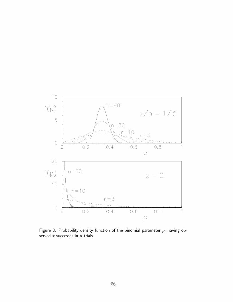
Figure 8: Probability density function of the binomial parameter p, having ob-served x successes in n trials.
56

when measuring efficiencies, branching ratios, etc. Stated more generally, onetries to infer the “constant and unknown probability”14 of an event occurring.
Where we can assume that the probability is constant and the observednumber of favorable events are binomially distributed, the unknown quantityto be measured is the parameter p of the binomial. Using Bayes’ theorem weget
f(p|x, n,B) =f(x|Bn,p)f(p)
∫ 1
0f(x|Bn,p)f(p)dp
=
n!(n−x)!x!
px(1 − p)n−xf(p)∫ 1
0n!
(n−x)!x!px(1 − p)n−xf(p)dp
=px(1 − p)n−x
∫ 1
0px(1 − p)n−xdp
, (134)
where an initial uniform distribution has been assumed. The final distri-bution is known to statisticians as β distribution since the integral at thedenominator is the special function called β, defined also for real values of xand n (technically this is a β with parameters a = x + 1 and b = n− x + 1).In our case these two numbers are integer and the integral becomes equal tox!(n − x)!/(n + 1)!. We then get
f(p|x, n,B) =(n + 1)!
x!(n − x)!px(1 − p)n−x . (135)
14This concept, which is very close to the physicist’s mentality, is not correct from theprobabilistic - cognitive - point of view. According to the Bayesian scheme, in fact, theprobability changes with the new observations. The final inference of p, however, does notdepend on the particular sequence yielding x successes over n trials. This can be seen inthe next table where fn(p) is given as a function of the number of trials n, for the threesequences which give 2 successes (indicated by “1”) in three trials (the use of (135) isanticipated):
Sequencen 011 101 1100 1 1 11 2(1 − p) 2p 2p2 6p(1 − p) 6p(1 − p) 3p2
3 12p2(1 − p) 12p2(1 − p) 12p2(1 − p)
This important result, related to the concept of interchangeability, “allows” a physicist whois reluctant to give up the concept “unknown constant probability”, to see the problemfrom his point of view, ensuring that the same numerical result is obtained.
57
The expected value and the variance of this distribution are:
E[p] =x + 1
n + 2(136)
V ar(p) =(x + 1)(n − x + 1)
(n + 3)(n + 2)2(137)
=x + 1
n + 2
(n
n + 2− x + 1
n + 2
)1
n + 3
= E[p]
(n
n + 2− E[p]
)1
n + 3. (138)
The value of p for which f(p) has the maximum is instead pm = x/n. Theexpression E[p] gives the prevision of the probability for the (n+1)-th eventoccurring and is called the “recursive Laplace formula”, or “Laplace’s rule ofsuccession”.
When x and n become large, and 0 ≪ x ≪ n, f(p) has the followingasymptotic properties:
E[p] ≈ pm =x
n; (139)
V ar(p) ≈ x
n
(1 − x
n
) 1
n=
pm(1 − pm)
n; (140)
σp ≈√
pm(1 − pm)
n: (141)
p ∼ N (pm, σp) . (142)
Under these conditions the frequentistic “definition” of probability (x/n) isrecovered.
Let us see two particular situations: when x = 0 and x = n. In thesecases one gives the result as upper or lower limits, respectively. Let us sketchthe solutions:
• x=n:
f(n|Bn,p) = pn; (143)
f(p|x = n,B) =pn
∫ 1
0pndp
= (n + 1) · pn; (144)
F (p|x = n,B) = pn+1 . (145)
To get the 95 % lower bound (limit):
F (p|x = n,B) = 0.05 ,
p =n+1√
0.05 . (146)
58

An increasing number of trials n constrain more and more p around 1.
• x=0:
f(0|Bn,p) = (1 − p)n; (147)
f(p|x = 0, n,B) =(1 − p)n
∫ 1
0(1 − p)ndp
= (n + 1) · (1 − p)n; (148)
F (p|x = 0, n,B) = 1 − (1 − p)n+1 . (149)
To get the 95 % upper bound (limit):
F (p|x = 0, n,B) = 0.95;
p = 1 − n+1√
0.05 . (150)
The following table shows the 95 % C.L. limits as a function of n. ThePoisson approximation, to be discussed in the next section, is also shown.
Probability level = 95 %n x = n x = 0
binomial binomial Poisson approx.( p = 3/n )
3 p ≥ 0.47 p ≤ 0.53 p ≤ 15 p ≥ 0.61 p ≤ 0.39 p ≤ 0.6
10 p ≥ 0.76 p ≤ 0.24 p ≤ 0.350 p ≥ 0.94 p ≤ 0.057 p ≤ 0.06
100 p ≥ 0.97 p ≤ 0.029 p ≤ 0.031000 p ≥ 0.997 p ≤ 0.003 p ≤ 0.003
To show in this simple case how f(p) is updated by the new information,let us imagine we have performed two experiments. The results are x1 = n1
and x2 = n2, respectively. Obviously the global information is equivalent tox = x1 + x2 and n = n1 + n2, with x = n. We then get
f(p|x = n,B) = (n + 1)pn = (n1 + n2 + 1)pn1+n2 . (151)
A different way of proceeding would have been to calculate the final distri-bution from the information x1 = n1
f(p|x1 = n1,B) = (n1 + 1)pn1 , (152)
59

and feed it as initial distribution to the next inference:
f(p|x1 = n1, x2 = n2,B) =pn2f(p|x1 = n1,B)
∫ 1
0pn2f(p|x1 = n1,B)dp
(153)
=pn2(n1 + 1)pn1
∫ 1
0pn2(n1 + 1)pn1dp
(154)
= (n1 + n2 + 1)pn1+n2 , (155)
getting the same result.
12.2 Poisson distributed quantities
As is well known, the typical application of the Poisson distribution is incounting experiments such as source activity, cross sections, etc. The un-known parameter to be inferred is λ. Applying Bayes formula we get
f(λ|x,P) =λxe−λ
x!f(λ)
∫∞0
λxe−λ
x!f(λ)dλ
. (156)
Assuming15 f(λ) constant up to a certain λmax ≫ x and making the integralby parts we obtain
f(λ|x,P) =λxe−λ
x!(157)
F (λ|x,P) = 1 − e−λ
(x∑
n=0
λn
n!
), (158)
where the last result has been obtained integrating (157) also by parts. Fig. 9shows how to build the credibility intervals, given a certain measured numberof counts x. Fig. 10 shows some numerical examples.
f(λ) has the following properties:
• the expected values, variance, value of maximum probability are
E[λ] = x + 1 (159)
V ar(λ) = x + 2 (160)
λm = x ; (161)15There is a school of thought according to which the most appropriate function is
f(λ) ∝ 1/λ. If You think that it is reasonable for your problem, it may be a goodprior. Claiming that this is “the Truth” is one of the many claims of the angels’ sexdeterminations. For didactical purposes a uniform distribution is more than enough.Some comments about the 1/λ prescription will be given when discussing the particularcase x = 0.
60

f( x2)
f( x1)
x1 x2
f( )
Figure 9: Poisson parameter λ inferred from an observed number x of counts.
the fact that the best estimate of λ in the Bayesian sense is not theintuitive value x but x + 1 should neither surprise, nor disappoint us:according to the initial distribution used “there are always more pos-sible values of λ on the right side than on the left side of x”, and theypull the distribution to their side; the full information is always givenby f(λ) and the use of the mean is just a rough approximation; thedifference from the “desired” intuitive value x in units of the standarddeviation goes as 1/
√n + 2 and becomes immediately negligible;
• when x becomes large we get:
E[λ] ≈ λm = x ; (162)
V ar(λ) ≈ λm = x ; (163)
σλ ≈ √x ; (164)
λ ∼ N (x,√
x) . (165)
(164) is one of the most familar formulae used by physicists to assessthe uncertainty of a measurement, although it is sometimes misused.
Let us conclude with a special case: x = 0. As one might imagine, theinference is highly sensitive to the initial distribution. Let us assume thatthe experiment was planned with the hope of observing something, i.e. thatit could detect a handful of events within its lifetime. With this hypothesisone may use any vague prior function not strongly peaked at zero. We havealready come across a similar case in section 11.3, concerning the upper limit
61

Figure 10: Examples of f(λ|xi).
of the neutrino mass. There it was shown that reasonable hypotheses basedon the positive attitude of the experimentalist are almost equivalent and thatthey give results consistent with detector performances. Let us use then theuniform distribution
f(λ|x = 0,P) = e−λ (166)
F (λ|x = 0,P) = 1 − e−λ (167)
λ < 3 at 95 % C.L. . (168)
13 Uncertainty due to unknown systematic
errors
13.1 Example: uncertainty of the instrument scale off-
set
In our scheme any quantity of influence of which we don’t know the exactvalue is a source of systematic error. It will change the final distribution of µand hence its uncertainty. We have already discussed the most general casein 9.1. Let us make a simple application making a small variation to theexample in section 11.1: the “zero” of the instrument is not known exactly,
62

1 -
1 2 3
95%
f( )
Figure 11: Upper limit to λ having observed 0 events.
owing to calibration uncertainty. This can be parametrized assuming thatits true value Z is normally distributed around 0 (i.e. the calibration wasproperly done!) with a standard deviation σZ . Since, most probably, thetrue value of µ is independent from the true value of Z, the initial jointprobability density function can be written as the product of the marginalones:
f(µ, z) = f(µ)f(z) = k1√
2πσZ
exp
[− z2
2σ2Z
]. (169)
Also the likelihood changes with respect to 114:
f(x1|µ, z) =1√
2πσ1
exp
[−(x1 − µ − z)2
2σ21
]. (170)
Putting all the pieces together and making use of (105) we finally get
f(µ|x1, . . . , f(z)) =
∫1√
2πσ1exp
[− (x1−µ−z)2
2σ21
]1√
2πσZexp
[− z2
2σ2Z
]dz
∫∫1√
2πσ1exp
[− (x1−µ−z)2
2σ21
]1√
2πσZexp
[− z2
2σ2Z
]dµdz
.
Integrating16 we get
f(µ) = f(µ|x1, . . . , f(z)) =1√
2π√
σ21 + σ2
Z
exp
[− (µ − x1)
2
2(σ21 + σ2
Z)
].(171)
16It may help to know that∫ +∞
−∞
exp
[bx − x2
a2
]dx =
√a2π exp
[a2b2
4
].
63

The result is that f(µ) is still a gaussian, but with a larger variance. Theglobal standard uncertainty is the quadratic combination of that due to thestatistical fluctuation of the data sample and the uncertainty due to theimperfect knowledge of the systematic effect:
σ2tot = σ2
1 + σ2Z . (172)
This result is well known, although there are still some “old-fashioned”recipes which require different combinations of the contributions to be per-formed.
One has to notice that in this framework it makes no sense to speak of“statistical” and “systematical” uncertainties, as if they were of a differentnature. They have the same probabilistic nature: Qn1
is around µ with astandard deviation σ1, and Z is around 0 with standard deviation σZ . Whatdistinguishes the two components is how the knowledge of the uncertaintyis gained: in one case (σ1) from repeated measurements; in the second case(σZ) the evaluation was done by somebody else (the constructor of the in-strument), or in a previous experiment, or guessed from the knowledge ofthe detector, or by simulation, etc. This is the reason why the ISO Guide [2]prefers the generic names Type A and Type B for the two kinds of contribu-tion to global uncertainty. In particular the name “systematic uncertainty”should be avoided, while it is correct to speak about “uncertainty due to asystematic effect”.
13.2 Correction for known systematic errors
It is easy to be convinced that if our prior knowledge about Z was of thekind
Z ∼ N (z, σZ) (173)
the result would have been
µ ∼ N(
x1 − z,√
σ21 + σ2
Z
), (174)
i.e. one has first to correct the result for the best value of the systematic errorand then include in the global uncertainty a term due to imperfect knowledgeabout it. This is a well known and practised procedure, although there arestill people who confuse z with its uncertainty.
64

13.3 Measuring two quantities with the same instru-ment having an uncertainty of the scale offset
Let us take an example which is a bit more complicated (at least from themathematical point of view) but conceptually very simple and also very com-mon in laboratory practice. We measure two physical quantities with thesame instrument, assumed to have an uncertainty on the “zero”, modeledwith a normal distribution as in the previous sections. For each of the quan-tities we collect a sample of data under the same conditions, which meansthat the unknown offset error does not change from one set of measurementsto the other. Calling µ1 and µ2 the true values, x1 and x2 the sample aver-ages, σ1 and σ2 the average’s standard deviations, and Z the true value ofthe “zero”, the initial probability density and the likelihood are
f(µ1, µ2, z) = f(µ1)f(µ2)f(z) = k1√
2πσZ
exp
[− z2
2σ2Z
]
(175)
and
f(x1, x2|µ1, µ2, z) =1√
2πσ1
exp
[−(x1 − µ1 − z)2
2σ21
]1√
2πσ2
exp
[−(x2 − µ2 − z)2
2σ22
]
=1
2πσ1σ2
exp
[−1
2
((x1 − µ1 − z)2
σ21
+(x2 − µ2 − z)2
σ22
)], (176)
respectively. The result of the inference is now the joint probability densityfunction of µ1 and µ2:
f(µ1, µ2|x1, x2, σ1, σ2, f(z)) =
∫f(x1, x2|µ1, µ2, z)f(µ1, µ2, z)dz∫∫∫
f(x1, x2|µ1, µ2, z)f(µ1, µ2, z)dµ1dµ2dz,(177)
where expansion of the functions has been omitted for the sake of clarity.Integrating we get
f(µ1, µ2) =1
2π√
σ21 + σ2
Z
√σ2
2 + σ2Z
√1 − ρ2
(178)
exp
− 1
2(1 − ρ2)
[(µ1 − x1)
2
σ21 + σ2
Z
− 2ρ(µ1 − x1)(µ2 − x2)√σ2
1 + σ2Z
√σ2
2 + σ2Z
+(µ2 − x2)
2
σ22 + σ2
Z
].
where
ρ =σ2
Z√σ2
1 + σ2Z
√σ2
2 + σ2Z
. (179)
65

If σZ vanishes then (178) has the simpler expression
f(µ1, µ2) −−−→σZ→0
1√2πσ1
exp
[−(µ1 − x1)
2
2σ21
]1√
2πσ2
exp
[−(µ2 − x2)
2
2σ22
],
(180)
i.e. if there is no uncertainty on the offset calibration the joint density func-tion then f(µ1, µ2) is equal to the product of two independent normal func-tions, i.e. µ1 and µ2 are independent. In the general case we have to concludethat:
• the effect of the common uncertainty σZ makes the two values correlated,since they are affected by a common unknown systematic error; thecorrelation coefficient is always non negative (ρ ≥ 0), as intuitivelyexpected from the definition of systematic error;
• the joint density function is a multinormal distribution of parametersx1, σµ1 =
√σ2
1 + σ2Z , x2, σµ2 =
√σ2
2 + σ2Z , and ρ (see example of
Fig. 5);
• the marginal distributions are still normal:
µ1 ∼ N(
x1,√
σ21 + σ2
Z
)(181)
µ2 ∼ N(
x2,√
σ22 + σ2
Z
); (182)
• the covariance between µ1 and µ2 is
Cov(µ1, µ2) = ρσµ1σµ2
= ρ√
σ21 + σ2
Z
√σ2
2 + σ2Z = σ2
Z . (183)
• the distribution of any function g(µ1, µ2) can be calculated using thestandard methods of probability theory. For example, one can demon-strate that the sum S = µ1 + µ2 and the difference D = µ1 − µ2 arealso normally distributed (see also the introductory discussion to thecentral limit theorem and section 16 for the calculation of averages andstandard deviations):
S ∼ N(
x1 + x2,√
σ21 + σ2
2 + (2σZ)2
)(184)
D ∼ N(
x1 − x2,√
σ21 + σ2
2
). (185)
The result can be interpreted in the following way:
66

– the uncertainty on the difference does not depend on the commonoffset uncertainty: whatever the value of the true “zero” is, itcancels in differences;
– in the sum, instead, the effect of the common uncertainty is some-what amplified since it enters “in phase” in the global uncertaintyof each of the quantities.
13.4 Indirect calibration
Let us use the result of the previous section to solve another typical problemof measurements. Suppose that after (or before, it doesn’t matter) we havedone the measurements of x1 and x2 and we have the final result, summarizedin (178), we know the “exact” value of µ1 (for example we perform themeasurement on a reference). Let us call it µ
1. Will this information providea better knowledge of µ2? In principle yes: the difference between x1 andµ
1 defines the systematic error (the true value of the “zero” Z). This errorcan then be subtracted from µ2 to get a corrected value. Also the overalluncertainty of µ2 should change, intuitively it “should” decrease, since weare adding new information. But its value doesn’t seem to be obvious, sincethe logical link between µ
1 and µ2 is µ1 → Z → µ2.
The problem can be solved exactly using the concept of conditional prob-ability density function f(µ2|µ
1) (see (93-94)). We get
µ2|µ
1∼N
x2 +σ2
Z
σ21 + σ2
Z
(µ1 − x1),
√
σ22 +
(1
σ21
+1
σ2Z
)−1
.(186)
The best value of µ2 is shifted by an amount ∆, with respect to the measuredvalue x2, which is not exactly x1 − µ
1, as was naıvely guessed, and theuncertainty depends on σ2, σZ and σ1. It is easy to be convinced that theexact result is more resonable than the (suggested) first guess. Let us rewrite∆ in two different ways:
∆ =σ2
Z
σ21 + σ2
Z
(µ1 − x1) (187)
=1
1σ21
+ 1σ2
Z
[1
σ21
· (x1 − µ1) +
1
σ2Z
· 0]
. (188)
• Eq. (187) shows that one has to apply the correction x1 − µ1 only if
σ1 = 0. If instead σZ = 0 there is no correction to be applied, since theinstrument is perfectly calibrated. If σ1 ≈ σZ the correction is half ofthe measured difference between x1 and µ
1;
67
• Eq. (188) shows explicitly what is going on and why the result isconsistent with the way we have modeled the uncertainties. In factwe have performed two independent calibrations: one of the offset andone of µ1. The best estimate of the true value of the “zero” Z is theweighted average of the two measured offsets;
• the new uncertainty of µ2 (see (186)) is a combination of σ2 and the un-certainty of the weighted average of the two offsets. Its value is smallerthan what one would have with only one calibration and, obviously,larger than that due to the sampling fluctuations alone:
σ2 ≤√
σ22 +
σ21σ
2Z
σ21 + σ2
Z
≤√
σ22 + σ2
Z . (189)
13.5 Counting measurements in presence of background
As an example of a different kind of systematic effect, let us think of countingexperiments in the presence of background. For example we are searchingfor a new particle, we make some selection cuts and count x events. Butwe also expect an average number of background events λB
± σB, where σB
is the standard uncertainty of λB, not to be confused with
√λB
. Whatcan we say about λS, the true value of the average number associated tothe signal? First we will treat the case on which the determination of theexpected number of background events is well known (σB/λB
≪ 1), andthen the general case:
σB/λB≪ 1 : the true value of the sum of signal and background is λ =
λS + λB. The likelihood is
P (x|λ) =e−λλx
x!. (190)
Applying Bayes’s theorem we have
f(λS|x, λB) =
e−(λB+λS)(λB
+ λS)xf(λS)∫∞0
e−(λB+λS)(λB
+ λS)xf(λS)dλS
. (191)
Choosing again f(λS) uniform (in a reasonable interval) this gets sim-plified. The integral at the denominator can be done easily by partsand the final result is:
f(λS|x, λB) =
e−λS(λB+ λS)x
x!∑x
n=0
λnB
n!
(192)
F (λS|x, λB) = 1 − e−λS
∑xn=0
(λB+λS)n
n!∑xn=0
λnB
n!
. (193)
68

From (192-193) it is possible to calculate in the usual way the bestestimate and the credibility intervals of λS. Two particular cases areof interest:
• if λB= 0 then formulae (157-158) are recovered. In such a case
one measured count is enough to claim for a signal (if somebody iswilling to believe that really λB
= 0 without any uncertainty. . . );
• if x = 0 then
f(λ|x, λB) = e−λS , (194)
independently of λB. This result is not really obvious.
Any g(λB) : In the general case, the true value of the average number of
background events λB is unknown. We only known that it is distributedaround λB
with standard deviation σB and probability density functiong(λB), not necessarily a gaussian. What changes with respect to theprevious case is the initial distribution, now a joint function of λS andof λB. Assuming λB and λS independent the prior density function is
f(λS, λB) = f(λS)g(λB) . (195)
We leave f in the form of a joint distribution to indicate that the resultwe shall get is the most general for this kind of problem. The likelihood,on the other hand, remains the same as in the previous example. Theinference of λS is done in the usual way, applying Bayes’ theorem andmarginalizing with respect to λS:
f(λS|x, g(λB)) =
∫e−(λB+λS)(λB + λS)xf(λS, λB)dλB∫∫
e−(λB+λS)(λB + λS)xf(λS, λB)dλSdλB
.(196)
The previous case (formula (192)) is recovered if the only value allowedfor λB is λB
and f(λS) is uniform:
f(λS, λB) = kδ(λB − λB) . (197)
14 Approximate methods
14.1 Linearization
We have seen in the above examples how to use the general formula (105)for practical applications. Unfortunately, when the problem becomes more
69

complicated one starts facing integration problems. For this reason approx-imate methods are generally used. We will derive the approximation rulesconsistently with the approach followed in these notes and then the resultingformulae will be compared with the ISO recommendations. To do this, let usneglect for a while all quantities of influence which could produce unknownsystematic errors. In this case (105) can be replaced by (106), which canbe further simplified if we remember that correlations between the resultsare originated by unknown systematic errors. In absence of these, the jointdistribution of all quantities µ is simply the product of marginal ones:
fRi(µi) =
∏
i
fRi(µi) , (198)
with
fRi(µi) = fRi
(µi|xi, h) =f(xi|µi, h)f(µi)∫f(xi|µi, h)f(µi)dµi
. (199)
The symbol fRi(µi) indicates that we are dealing with raw values17 evaluated
at h = h. Since for any variation of h the inferred values of µi will change,it is convenient, to name with the same subscript R the quantity obtainedfor h:
fRi(µi) −→ fRi
(µRi) . (200)
Let us indicate with µRiand σRi
the best estimates and the standarduncertainty of the raw values:
µRi= E[µRi
] (201)
σ2Ri
= V ar(µRi) . (202)
For any possible configuration of conditioning hypotheses h, corrected valuesµi are obtained:
µi = µRi+ gi(h) . (203)
The function which relates the corrected value to the raw value and to thesystematic effects has been denoted by gi not to be confused with a proba-bility density function. Expanding (203) in series around h we finally arriveat the expression which will allow us to make the approximated evaluationsof uncertainties:
µi = µRi+∑
l
∂gi
∂hl(hl − hl
) + . . . (204)
17The choice of the adjective “raw” will become clearer in a later on.
70

(All derivatives are evaluated at µRi, h. To simplify the notation a similar
convention will be used in the following formulae).Neglecting the terms of the expansion above the first order, and taking
the expected values, we get
µi = E[µi]
≈ µRi; (205)
σ2µi
= E[(µi − E[µi])
2]
≈ σ2Ri
+∑
l
(∂gi
∂hl
)2
σ2hl
+2∑
l<m
(∂gi
∂hl
)(∂gi
∂hm
)ρlmσhl
σhm
; (206)
Cov(µi, µj) = E [(µi − E[µi])(µj − E[µj ])]
≈∑
l
(∂gi
∂hl
)(∂gj
∂hl
)σ2
hl
+2∑
l<m
(∂gi
∂hl
)(∂gj
∂hm
)ρlmσhl
σhm
. (207)
The terms included within · vanish if the unknown systematic errors areuncorrelated, and the formulae become simpler. Unfortunately, very oftenthis is not the case, as when several calibration constants are simultaneouslyobtained from a fit (for example, in most linear fits slop and intercept havea correlation coefficient close to −0.9).
Sometimes the expansion (204) is not performed around the best valuesof h but around their nominal values, in the sense that the correction for theknown value of the systematic errors has not yet been applied (see section13.2). In this case (204) should be replaced by
µi = µRi+∑
l
∂gi
∂hl
(hl − hNl) + . . . (208)
where the subscript N stands for nominal. The best value of µi is then
µi = E[µi]
≈ µRi+ E
[∑
l
∂gi
∂hl(hl − hNl
)
]
= µRi+∑
l
δµil . (209)
71

(206) and (207) instead remain valid, with the condition that the derivativeis calculated at hN . If ρlm = 0 it is possible to rewrite (206) and (207) in thefollowing way, which is very convenient for practical applications:
σ2µi
≈ σ2Ri
+∑
l
(∂gi
∂hl
)2
σ2hl
(210)
= σ2Ri
+∑
l
u2il
; (211)
Cov(µi, µj) ≈∑
l
(∂gi
∂hl
)(∂gj
∂hl
)σ2
hl(212)
=∑
l
sijl
∣∣∣∣∂gi
∂hl
∣∣∣∣ σhl
∣∣∣∣∂gj
∂hl
∣∣∣∣ σhl(213)
=∑
l
sijluilujl
(214)
=∑
l
Covl(µi, µj) . (215)
uil is the component to the standard uncertainty due to effect hl. sijlis equal
to the product of signs of the derivatives, which takes into account whetherthe uncertainties are positively or negatively correlated.
To summarize, when systematic effects are not correlated with each other,the following quantities are needed to evaluate the corrected result, the com-bined uncertainties and the correlations:
• the raw µRiand σRi
;
• the best estimates of the corrections δµil for each systematic effect hl;
• the best estimate of the standard deviation uil due to the imperfectknowledge of the systematic effect;
• for any pair µi, µj the sign of the correlation sijldue to the effect hl.
In High Energy Physics applications it is frequently the case that thederivatives appearing in (209-213) cannot be calculated directly, as for ex-ample when hl are parameters of a simulation program, or acceptance cuts.Then variations of µ
iare usually studied varying a particular hl within a rea-
sonable interval, holding the other influence quantities at the nominal value.δµil and uil are calculated from the interval ±∆±
i of variation of the truevalue for a given variation ±∆±
hlof hl and from the probabilistic meaning of
72

the intervals (i.e. from the assumed distribution of the true value). This em-pirical procedure for determining δµil and uil has the advantage that it cantake into account non linear effects, since it directly measures the differenceµi − µRi
for a given difference hl − hNl.
Some examples are given in section 14.4, and two typical experimentalapplications will be discussed in more detail in section 16.
14.2 BIPM and ISO recommendations
In this section we compare the results obtained in the previous sectionwith the recommendations of the Bureau International des Poids et Mesures(BIPM) and the International Organization for Standardization (ISO) on“the expression of experimental uncertainty”.
1. The uncertainty in the result of a measurement generally consistsof several components which may be grouped into two categoriesaccording to the way in which their numerical value is estimated:
A: those which are evaluated by statistical methods;
B: those which are evaluated by other means.
There is not always a simple correspondence between the classifi-cation into categories A or B and the previously used classificationinto “random” and “systematic” uncertainties. The term “sys-tematic uncertainty” can be misleading and should be avoided.
The detailed report of the uncertainty should consist of a com-
plete list of the components, specifying for each the method used
to obtain its numerical result.
Essentially the first recommendation states that all uncertainties canbe treated probabilistically. The distinction between types A and Bis subtle and can be misleading if one thinks of “statistical methods”as synonymous with “probabilistic methods” - as currently done inHigh Energy Physics. Here “statistical” has the classical meaning ofrepeated measurements.
2. The components in category A are characterized by the estimated
variances s2i (or the estimated “standard deviations” si) and the
number of degrees of freedom νi. Where appropriate, the covari-
ances should be given.
The estimated variances correspond to σ2Ri
of the previous section. Thedegrees of freedom have are related to small samples and to the Stu-dent t distribution. The problem of small samples is not discussed in
73

these notes, but clearly this recommendation is a relic of frequentisticmethods. With the approach followed in theses notes there is no needto talk about degrees of freedom, since the Bayesian inference definesthe final probability function f(µ) completely.
3. The components in category B should be characterized by quan-
tities u2j , which may be considered as approximations to the cor-
responding variances, the existence of which is assumed. The
quantities u2j may the treated like variances and the quantities
uj like standard deviations. Where appropriate, the covariances
should be treated in a similar way.
Clearly, this recommendation is meaningful only in a Bayesian frame-work.
4. The combined uncertainty should be characterized by the numeri-
cal value obtained by applying the usual method for the combina-
tion of variances. The combined uncertainty and its components
should be expressed in the form of “standard deviations”.
This is what we have found in (206-207).
5. If, for particular applications, it is necessary to multiply the com-
bined uncertainty by a factor to obtain an overall uncertainty, the
multiplying factor used must always stated.
This last recommendation states once more that the uncertainty is “bydefault” the standard deviation of the true value distribution. Anyother quantity calculated to obtain a credibility interval with a certainprobability level should be clearly stated.
To summarize, these are the basic ingredients of the BIPM/ISO recommen-dations:
subjective definition of probability: it allows variances to be assignedconceptually to any physical quantity which has an uncertain value;
uncertainty as standard deviation
• it is “standard”;
• the rule of combination (85-88) applies to standard deviations andnot to confidence intervals;
combined standard uncertainty: it is obtained by the usual formula of“error propagation” and it makes use on variances, covariances andfirst derivatives;
74

central limit theorem: it makes, under proper conditions, the true valuenormally distributed if one has several sources of uncertainty.
Consultation of the Guide[2] is recommended for further explanationsabout the justification of the norms, for the description of evaluation proce-dures, as well for as examples. I would just like to end this section with someexamples of the evaluation of type B uncertainties and with some words ofcaution concerning the use of approximations and of linearization.
14.3 Evaluation of type B uncertainties
The ISO Guide states that
For estimate xi of an input quantity18 Xi that has not been obtainedfrom repeated observations, the . . . standard uncertainty ui is evalu-ated by scientific judgement based on all the available information onthe possible variability of Xi. The pool of information may include
• previous measurement data;
• experience with or general knowledge of the behaviour and prop-erties of relevant materials and instruments;
• manufacturer’s specifications;
• data provided in calibration and other certificates;
• uncertainties assigned to reference data taken from handbooks.
14.4 Examples of type B uncertainties
1. A manufacturer’s calibration certificate states that the uncertainty, de-fined as k standard deviations, is “±∆”:
u =∆
k.
2. A result is reported in a publication as x±∆, stating that the averagehas been performed on 4 measurements and the uncertainty is a 95 %confidence interval. One has to conclude that the confidence intervalhas been calculated using the Student t:
u =∆
3.18.
18By “input quantity” the ISO Guide mean any of the contributions hl or µRiwhich
enter into (206-207).
75
3. a manufacturer’s specification states that the error on a quantity shouldnot exceed ∆. With this limited information one has to assume auniform distribution:
u =2∆√12
=∆√3
;
4. A physical parameter of a Monte Carlo is believed to lie in the interval of±∆ around its best value, but not with uniform distribution: the proba-bility that the parameter is at center is higher than than that it is at theedges of the interval. With this information a triangular distributioncan be reasonably assumed:
u =∆√6
.
Note that the coefficient in front of ∆ changes from the 0.58 of the pre-vious example to the 0.41 of this. If the interval ±∆ were a 3σ intervalthen the coefficient would have been equal to 0.33. These variations -to be considered extreme - are smaller than the statistical fluctuationsof empirical standard deviations estimated from ≈ 10 measurements.This shows that one should not be worried that the type B uncertain-ties are less accurate than type A, especially if one tries to model thedistribution of the physical quantity honestly.
5. The absolute energy calibration of an electromagnetic calorimeter mod-ule is not exactly known and it is estimated to be between the nominalone and +10 %. The “statistical” resolution is known by test beammeasurements to be 18%/
√E/GeV. What is the uncertainty on the
energy measurement of an electron which has apparently released 30GeV?
• The energy has to be corrected for the best estimate of the cali-bration constant: +5 %:
ER = 31.5 ± 1.0 GeV .
– assuming a uniform distribution of the true calibration con-stant: u = 31.5 × 0.1/
√12 = 0.9 GeV:
E = 31.5 ± 1.3 GeV ;
– assuming a triangular distribution: u = 1.3 GeV:
E = 31.5 ± 1.6 GeV ;
76
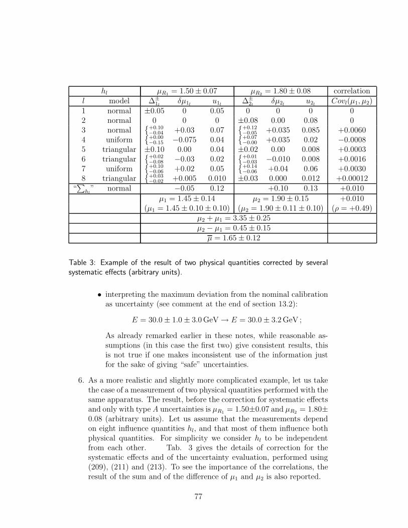
hl µR1 = 1.50 ± 0.07 µR2 = 1.80 ± 0.08 correlationl model ∆±
1lδµ1l
u1l∆±
2lδµ2l
u2lCovl(µ1, µ2)
1 normal ±0.05 0 0.05 0 0 0 02 normal 0 0 0 ±0.08 0.00 0.08 03 normal
+0.10−0.04 +0.03 0.07
+0.12−0.05 +0.035 0.085 +0.0060
4 uniform
+0.00−0.15 −0.075 0.04
+0.07−0.00 +0.035 0.02 −0.0008
5 triangular ±0.10 0.00 0.04 ±0.02 0.00 0.008 +0.00036 triangular
+0.02−0.08 −0.03 0.02
+0.01−0.03 −0.010 0.008 +0.0016
7 uniform
+0.10−0.06 +0.02 0.05
+0.14−0.06 +0.04 0.06 +0.0030
8 triangular
+0.03−0.02 +0.005 0.010 ±0.03 0.000 0.012 +0.00012
“∑
hl” normal −0.05 0.12 +0.10 0.13 +0.010
µ1 = 1.45 ± 0.14 µ2 = 1.90 ± 0.15 +0.010(µ1 = 1.45 ± 0.10 ± 0.10) (µ2 = 1.90 ± 0.11 ± 0.10) (ρ = +0.49)
µ2 + µ1 = 3.35 ± 0.25µ2 − µ1 = 0.45 ± 0.15
µ = 1.65 ± 0.12
Table 3: Example of the result of two physical quantities corrected by severalsystematic effects (arbitrary units).
• interpreting the maximum deviation from the nominal calibrationas uncertainty (see comment at the end of section 13.2):
E = 30.0 ± 1.0 ± 3.0 GeV → E = 30.0 ± 3.2 GeV ;
As already remarked earlier in these notes, while reasonable as-sumptions (in this case the first two) give consistent results, thisis not true if one makes inconsistent use of the information justfor the sake of giving “safe” uncertainties.
6. As a more realistic and slightly more complicated example, let us takethe case of a measurement of two physical quantities performed with thesame apparatus. The result, before the correction for systematic effectsand only with type A uncertainties is µR1 = 1.50±0.07 and µR2 = 1.80±0.08 (arbitrary units). Let us assume that the measurements dependon eight influence quantities hl, and that most of them influence bothphysical quantities. For simplicity we consider hl to be independentfrom each other. Tab. 3 gives the details of correction for thesystematic effects and of the uncertainty evaluation, performed using(209), (211) and (213). To see the importance of the correlations, theresult of the sum and of the difference of µ1 and µ2 is also reported.
77

In order to split the final result into “individual” and “common” un-certainty (between parenthesis in Tab. 3) we have to remember that,if the error is additive, the covariance between µ1 and µ2 is given bythe variance of the unknown systematic error (see 183).
The average µ between µ1 and µ2, assuming it has a physical meaning,can be evaluated either using the results of section 16, or simply calcu-lating the average weighted with the inverse of the variances due to theindividual uncertainties, and then adding quadratically the commonuncertainty at the end. Also µ is reported in Tab. 3.
14.5 Caveat concerning a blind use of approximate
methods
The mathematical apparatus of variances and covariances of (206-207) isoften seen as the most complete description of uncertainty and in most casesused blindly in further uncertainty calculations. It must be clear, however,that this is just an approximation based on linearization. If the functionwhich relates the corrected value to the raw value and the systematic effectsis not linear then the linearization may cause trouble. An interesting case isdiscussed in section 16.
There is another problem which may arise from the simultaneous use ofBayesian estimators and approximate methods. Let us introduce the problemwith an example.
Example 1: 1000 independent measurements of the efficiency of a detectorhave been performed (or 1000 measurements of branching ratio, if youprefer). Each measurement was carried out on a base of 100 events andeach time 10 favorable events were observed (this obviously strange -though not impossible - but it simplifies the calculations). The resultof each measurement will be (see (136-138)):
ǫi =10 + 1
100 + 2= 0.1078 (216)
σ(ǫi) =
√11 · 91
103 · 1022= 0.031 ; (217)
Combining the 1000 results using the standard weighted average pro-cedure gives
ǫ = 0.1078 ± 0.0010 . (218)
78

Alternatively, taking the complete set of results to be equivalent to100000 trials with 10000 favorable events, the combined result is
ǫ′ = 0.10001 ± 0.0009 . (219)
(the same as if one had used the Bayes theorem iteratively to infer f(ǫ)from the the partial 1000 results.) The conclusions are in disagreementand the first result is clearly mistaken.
The same problem arises in the case of inference of the Poisson distributionparameter λ and, in general, whenever f(µ) is not symmetrical around E[µ].
Example 2: Imagine an experiment running continuously for one year, search-ing for monopoles and identifying none. The consistency with zero canbe stated either quoting E[λ] = 1 and σλ = 2, or a 95 % upper limitλ < 3. In terms of rate (number of monopoles per day) the resultwould be either E[r] = 2.7 · 10−3, σ(r) = 5.5 · 10−3, or an upper limitr < 8.2 ·10−3. It easy to show that, if we take the 365 results for each ofthe running days and combine them using the standard weighted aver-age, we get r = 1.0± 0.1 monopoles/day! This absurdity is not causedby the Bayesian method, but by the standard rules for combining theresults (the weighted average formulae (122) and (123) are derived fromthe normal distribution hypothesis). Using Bayesian inference wouldhave led to a consistent and reasonable result no matter how the 365days of running had been subdivided for partial analysis.
This suggests that in some cases it could be preferable to give the result interms of the value of µ which maximizes f(µ) (pm and λm of sections 12.1 and12.2). This way of presenting the results is similar to that suggested by themaximum likelihood approach, with the difference that for f(µ) one shouldtake the final probability density function and not simply the likelihood.Since it is practically impossible to summarize the outcome of an inferencein only two numbers (best value and uncertainty), a description of the methodused to evaluate them should be provided, except when f(µ) is approximatelynormally distributed (fortunately this happens most of the time).
15 Indirect measurements
Conceptually this is a very simple task in the Bayesian framework, whereasthe frequentistic one requires a lot of gymnastics going back and forward fromthe logical level of true values to the logical level of estimators. If one accepts
79

that the true values are just random variables19, then, calling Y a functionof other quantities X, each having a probability density function f(x), theprobability density function of Y f(y) can be calculated with the standardformulae which follow from the rules probability. Note that in the approachpresented in these notes uncertainties due to systematic effects are treated inthe same way as indirect measurements. It is worth repeating that there isno conceptual distinction between various components of the measurementuncertainty. When approximations are sufficient, formulae (206) and (207)can be used.
Let us take an example for which the linearization does not give the rightresult:
Example: The speed of a proton is measured with a time-of-flight system.Find the 68, 95 and 99 % probability intervals for the energy, knowingthat β = v/c = 0.9971, and that distance and time have been measuredwith a 0.2 % accuracy.
The relation
E =mc2
√1 − β2
is strongly non linear. The results given by the approximated methodand the correct one are, respectively:
C.L. linearization correct(%) E (GeV) E (GeV)68 6.4 ≤ E ≤ 18 8.8 ≤ E ≤ 6495 0.7 ≤ E ≤ 24 7.2 ≤ E < ∞99 0. ≤ E ≤ 28 6.6 ≤ E < ∞
16 Covariance matrix of experimental results
16.1 Building the covariance matrix of experimental
data
In physics applications, it is rarely the case that the covariance betweenthe best estimates of two physical quantities20, each given by the arithmetic
19To make the formalism lighter, let us call both the random variable associated to thequantity and the quantity itself by the same name Xi (instead of µxi
).20In this section[16] the symbol Xi will indicate the variable associated to the i-th
physical quantity and Xik its k-th direct measurement; xi the best estimate of its value,
80

average of direct measurements (xi = Xi = 1n
∑nk=1 Xik), can be evaluated
from the sample covariance of the two averages
Cov(xi, xj) =1
n(n − 1)
n∑
k=1
(Xik − X i)(Xjk − Xj) . (220)
More frequent is the well understood case in which the physical quantitiesare obtained as a result of a χ2 minimization, and the terms of the inverseof the covariance matrix are related to the curvature of χ2 at its minimum:
(V −1
)ij
=1
2
∂2χ2
∂Xi∂Xj
∣∣∣∣xi,xj
. (221)
In most cases one determines independent values of physical quantitieswith the same detector, and the correlation between them originates fromthe detector calibration uncertainties. Frequentistically, the use of (220) inthis case would correspond to having a “sample of detectors”, with each ofwhich a measurement of all the physical quantities is performed.
A way of building the covariance matrix from the direct measurementsis to consider the original measurements and the calibration constants as acommon set of independent and uncorrelated measurements, and then to cal-culate corrected values that take into account the calibration constants. Thevariance/covariance propagation will automatically provide the full covari-ance matrix of the set of results. Let us derive it for two cases that happenfrequently, and then proceed to the general case.
16.1.1 Offset uncertainty
Let xi ± σi be the i = 1 . . . n results of independent measurements and VX
the (diagonal) covariance matrix. Let us assume that they are all affectedby the same calibration constant c, having a standard uncertainty σc. Thecorrected results are then yi = xi +c. We can assume, for simplicity, that themost probable value of c is 0, i.e. the detector is well calibrated. One has toconsider the calibration constant as the physical quantity Xn+1, whose bestestimate is xn+1 = 0. A term VXn+1,n+1 = σ2
c must be added to the covariancematrix.
The covariance matrix of the corrected results is given by the transfor-mation:
VY = MVXMT , (222)
obtained by an average over many direct measurements or indirect measurements, σi thestandard deviation, and yi the value corrected for the calibration constants. The weightedaverage of several xi will be denoted by x.
81

where Mij = ∂Yi
∂Xj
∣∣∣xj
. The elements of VY are given by
VYkl=∑
ij
∂Yk
∂Xi
∣∣∣∣xi
∂Yl
∂Xj
∣∣∣∣xj
VXij. (223)
In this case we get:
σ2(Yi) = σ2i + σ2
c (224)
Cov(Yi, Yj) = σ2c (i 6= j) (225)
ρij =σ2
c√σ2
i + σ2c
√σ2
j + σ2c
(226)
=1√
1 +(
σi
σc
)2√
1 +(
σj
σc
)2, (227)
reobtaining the results of section 13.3. The total uncertainty on the singlemeasurement is given by the combination in quadrature of the individual andthe common standard uncertainties, and all the covariances are equal to σ2
c .To verify, in a simple case, that the result is reasonable, let us consider onlytwo independent quantities X1 and X2, and a calibration constant X3 = c,having an expected value equal to zero. From these we can calculate thecorrelated quantities Y1 and Y2 and finally their sum (S ≡ Z1) and difference(D ≡ Z2). The results are:
VY =
(σ2
1 + σ2c σ2
c
σ2c σ2
2 + σ2c
)(228)
(229)
(230)
VZ =
(σ2
1 + σ22 + 4 · σ2
c σ21 − σ2
2
σ21 − σ2
2 σ21 + σ2
2
). (231)
It follows that
σ2(S) = σ21 + σ2
2 + (2 · σc)2 (232)
σ2(D) = σ21 + σ2
2 , (233)
as intuitively expected.
16.1.2 Normalization uncertainty
Let us consider now the case where the calibration constant is the scale factorf , known with a standard uncertainty σf . Also in this case, for simplicity
82

and without losing generality, let us suppose that the most probable value off is 1. Then Xn+1 = f , i.e. xn+1 = 1, and VXn+1,n+1 = σ2
f . Then
σ2(Yi) = σ2i + σ2
fx2i (234)
Cov(Yi, Yj) = σ2fxixj (i 6= j) (235)
ρij =xixj√
x2i +
σ2i
σ2f
√x2
j +σ2
j
σ2f
(236)
|ρij | =1√
1 +(
σi
σf xi
)2√
1 +(
σj
σf xj
)2(237)
. (238)
To verify the results let us consider two independent measurements X1 andX2, let us calculate the correlated quantities Y1 and Y2, and finally theirproduct (P ≡ Z1) and their ratio (R ≡ Z2):
VY =
σ2
1 + σ2f · x2
1 σ2f · x1 · x2
σ2f · x1 · x2 σ2
2 + σ2f · x2
(239)
(240)
(241)
VZ =
σ2
1 · x22 + σ2
2 · x21 + 4 · σ2
f · x21 · x2
2 σ21 − σ2
2 · x21
x22
σ21 − σ2
2 · x21
x22
σ21
x22
+ σ22 · x2
1
x42
. (242)
It follows that:
σ2(P ) = σ21 · x2
2 + σ22 · x2
1 + (2 · σf · x1 · x2)2 (243)
σ2(R) =σ2
1
x22
+ σ22 ·
x21
x42
. (244)
Just as an unknown common offset error cancels in differences and is en-hanced in sums, an unknown normalization error has a similar effect on theratio and the product. It is also interesting to calculate the standard uncer-tainty of a difference in case of a normalization error:
σ2(D) = σ21 + σ2
2 + σ2f · (x1 − x2)
2 . (245)
The contribution from an unknown normalization error vanishes if the twovalues are equal.
83

16.1.3 General case
Let us assume there are n independently measured values xi and m cali-bration constants cj with their covariance matrix Vc. The latter can also betheoretical parameters influencing the data, and moreover they may be corre-lated, as usually happens if, for example, they are parameters of a calibrationfit. We can then include the cj in the vector that contains the measurementsand Vc in the covariance matrix VX :
x =
x1...
xn
c1...
cm
, VX =
σ21 0 · · · 00 σ2
2 · · · 0· · · · · · · · · · · · 00 0 · · · σ2
n
0 Vc
.
(246)
The corrected quantities are obtained from the most general function
Yi = Yi(Xi, c) (i = 1, 2, . . . , n) , (247)
and the covariance matrix VY from the covariance propagation VY = MVXMT .As a frequently encountered example, we can think of several normaliza-
tion constants, each affecting a subsample of the data - as is the case whereeach of several detectors measures a set of physical quantities. Let us con-sider consider just three quantities (Xi) and three uncorrelated normalizationstandard uncertainties (σfj
), the first one common to X1 and X2, the secondto X2 and X3 and the third to all three. We get the following covariancematrix:
σ21 +
(σ2
f1+ σ2
f3
)· x2
1
(σ2
f1+ σ2
f3
)· x1 · x2 σ2
f3· x1 · x3
(σ2
f1+ σ2
f3
)· x1 · x2 σ2
2 +(σ2
f1+ σ2
f2+ σ2
f3
)· x2
2
(σ2
f2+ σ2
f3
)· x2 · x3
σ2f3· x1 · x3
(σ2
f2+ σ2
f3
)· x2 · x3 σ2
3 +(σ2
f2+ σ2
f3
)· x2
3
.
16.2 Use and misuse of the covariance matrix to fit
correlated data
16.2.1 Best estimate of the true value from two correlated values.
Once the covariance matrix is built one uses it in a χ2 fit to get the parametersof a function. The quantity to be minimized is χ2, defined as
χ2 = ∆TV−1∆ , (248)
84

where ∆ is the vector of the differences between the theoretical and theexperimental values. Let us consider the simple case in which two results ofthe same physical quantity are available, and the individual and the commonstandard uncertainty are known. The best estimate of the true value of thephysical quantity is then obtained by fitting the constant Y = k through thedata points. In this simple case the χ2 minimization can be performed easily.We will consider the two cases of offset and normalization uncertainty. Asbefore, we assume that the detector is well calibrated, i.e. the most probablevalue of the calibration constant is, respectively for the two cases, 0 and 1,and hence yi = xi
16.2.2 Offset uncertainty
Let x1 ± σ1 and x2 ± σ2 be the two measured values, and σc the commonstandard uncertainty. The χ2 is
χ2 =1
D
[(x1 − k)2 · (σ2
2 + σ2c ) + (x2 − k)2 · (σ2
1 + σ2c ) (249)
−2 · (x1 − k) · (x2 − k) · σ2c
], (250)
where D = σ21 ·σ2
2 +(σ21 +σ2
2) ·σ2c is the determinant of the covariance matrix.
Minimizing χ2 and using the second derivative calculated at the minimumwe obtain the best value of k and its standard deviation:
k =x1 · σ2
2 + x2 · σ21
σ21 + σ2
2
(= x) (251)
(252)
σ2(k) =σ2
1 · σ22
σ21 + σ2
2
+ σ2c . (253)
The most probable value of the physical quantity is exactly what one obtainsfrom the average x weighted with the inverse of the individual variances.Its overall uncertainty is the quadratic sum of the standard deviation of theweighted average and the common one. The result coincides with the simpleexpectation.
16.2.3 Normalization uncertainty
Let x1 ± σ1 and x2 ± σ2 be the two measured values, and σf the commonstandard uncertainty on the scale. The χ2 is
χ2 =1
D
[(x1 − k)2 · (σ2
2 + x22 · σ2
f ) + (x2 − k)2 · (σ21 + x2
1 · σ2f) (254)
−2 · (x1 − k) · (x2 − k) · x1 · x2 · σ2f
], (255)
85

where D = σ21 ·σ2
2 +(x21 ·σ2
2 +x22 ·σ2
1) ·σ2f . We obtain in this case the following
result:
k =x1 · σ2
2 + x2 · σ21
σ21 + σ2
2 + (x1 − x2)2 · σ2f
(256)
(257)
σ2(k) =σ2
1 · σ22 + (x2
1 · σ22 + x2
2 · σ21) · σ2
f
σ21 + σ2
2 + (x1 − x2)2 · σ2f
. (258)
With respect to the previous case, k has a new term (x1 − x2)2 · σ2
f in thedenominator. As long as this is negligible with respect to the individualvariances we still get the weighted average x, otherwise a smaller value isobtained. Calling r the ratio between k and x, we obtain
r =k
x=
1
1 + (x1−x2)2
σ21+σ2
2· σ2
f
. (259)
Written in this way, one can see that the deviation from the simple averagevalue depends on the compatibility of the two values and on the normalizationuncertainty. This can be understood in the following way: as soon as thetwo values are in some disagreement, the fit starts to vary the normalizationfactor - in a hidden way - and to squeeze the scale by an amount allowed byσf , in order to minimize the χ2. The reason the fit prefers, normalizationfactors smaller than 1 under these conditions lies in the standard formalism ofthe covariance propagation, where only first derivatives are considered. Thisimplies that the individual standard deviations are not rescaled by loweringthe normalization factor, but the points get closer.
Example 1. Consider the results of two measurements, 8.0 · (1 ± 2 %) and8.5 · (1 ± 2 %), having a 10 % common normalization error. Assumingthat the two measurements refer to the same physical quantity, thebest estimate of its true value can be obtained by fitting the points toa constant. Minimizing χ2 with V estimated empirically by the data,as explained in the previous section, one obtains a value of 7.87± 0.81,which is surprising to say the least, since the most probable result isoutside the interval determined by the two measured values.
Example 2. A real life case of this strange effect which occurred duringthe global analysis of the R ratio in e+e− performed by the CELLOcollaboration[17], is shown in Fig. 12. The data points represent theaverages in energy bins of the results of the PETRA and PEP experi-ments. They are all correlated and the error bars show the total error
86

Figure 12: R measurements from PETRA and PEP experiments with the bestfits of QED+QCD to all the data (full line) and only below 36 GeV (dashed line).All data points are correlated (see text).
(see [17] for details). In particular, at the intermediate stage of theanalysis shown in the figure, an overall 1 % systematic error due the-oretical uncertainties was included in the covariance matrix. The Rvalues above 36 GeV show the first hint of the rise of the e+e− crosssection due to the Z pole. At that time it was very interesting toprove that the observation was not just a statistical fluctuation. Inorder to test this, the R measurements were fitted with a theoreticalfunction having no Z contributions, using only data below a certainenergy. It was expected that a fast increase of χ2 per number of degreesof freedom ν would be observed above 36 GeV, indicating that a the-oretical prediction without Z would be inadequate for describing thehigh energy data. The surprising result was a “repulsion” (see Fig. 12)between the experimental data and the fit: including the high energypoints with larger R a lower curve was obtained, while χ2/ν remainedalmost constant.
To see the source of this effect more explicitly let us consider an alterna-tive way often used to take the normalization uncertainty into account. Ascale factor f , by which all data points are multiplied, is introduced to theexpression of the χ2:
χ2A =
(f · x1 − k)2
(f · σ1)2+
(f · x2 − k)2
(f · σ2)2+
(f − 1)2
σ2f
. (260)
87
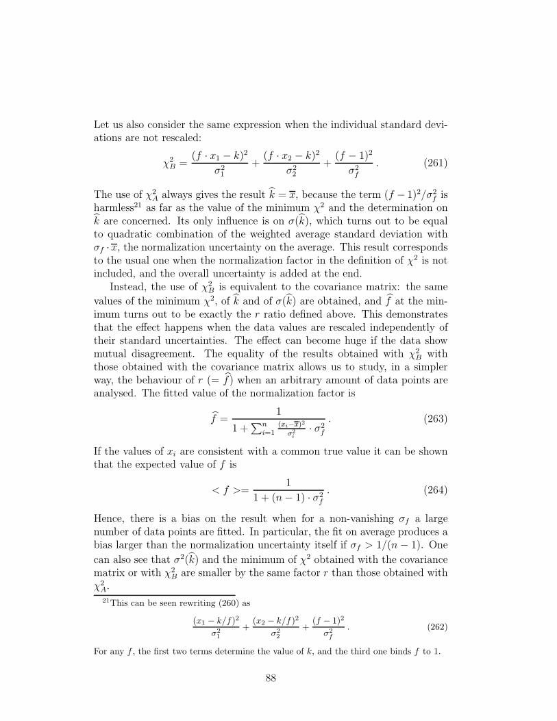
Let us also consider the same expression when the individual standard devi-ations are not rescaled:
χ2B =
(f · x1 − k)2
σ21
+(f · x2 − k)2
σ22
+(f − 1)2
σ2f
. (261)
The use of χ2A always gives the result k = x, because the term (f − 1)2/σ2
f isharmless21 as far as the value of the minimum χ2 and the determination onk are concerned. Its only influence is on σ(k), which turns out to be equalto quadratic combination of the weighted average standard deviation withσf ·x, the normalization uncertainty on the average. This result correspondsto the usual one when the normalization factor in the definition of χ2 is notincluded, and the overall uncertainty is added at the end.
Instead, the use of χ2B is equivalent to the covariance matrix: the same
values of the minimum χ2, of k and of σ(k) are obtained, and f at the min-imum turns out to be exactly the r ratio defined above. This demonstratesthat the effect happens when the data values are rescaled independently oftheir standard uncertainties. The effect can become huge if the data showmutual disagreement. The equality of the results obtained with χ2
B withthose obtained with the covariance matrix allows us to study, in a simplerway, the behaviour of r (= f) when an arbitrary amount of data points areanalysed. The fitted value of the normalization factor is
f =1
1 +∑n
i=1(xi−x)2
σ2i
· σ2f
. (263)
If the values of xi are consistent with a common true value it can be shownthat the expected value of f is
< f >=1
1 + (n − 1) · σ2f
. (264)
Hence, there is a bias on the result when for a non-vanishing σf a largenumber of data points are fitted. In particular, the fit on average produces abias larger than the normalization uncertainty itself if σf > 1/(n − 1). One
can also see that σ2(k) and the minimum of χ2 obtained with the covariancematrix or with χ2
B are smaller by the same factor r than those obtained withχ2
A.21This can be seen rewriting (260) as
(x1 − k/f)2
σ21
+(x2 − k/f)2
σ22
+(f − 1)2
σ2f
. (262)
For any f , the first two terms determine the value of k, and the third one binds f to 1.
88

16.2.4 Peelle’s Pertinent Puzzle
To summarize, where there is an overall uncertainty due to an unknown sys-tematic error and the covariance matrix is used to define χ2, the behaviourof the fit depends on whether the uncertainty is on the offset or on the scale.In the first case the best estimates of the function parameters are exactlythose obtained without overall uncertainty, and only the parameters’ stan-dard deviations are affected. In the case of unknown normalization errors,biased results can be obtained. The size of the bias depends on the fittedfunction, on the magnitude of the overall uncertainty and on the number ofdata points.
It has also been shown that this bias comes from the linearization per-formed in the usual covariance propagation. This means that, even thoughthe use of the covariance matrix can be very useful in analyzing the data ina compact way using available computer algorithms, care is required if thereis one large normalization uncertainty which affects all the data.
The effect discussed above has also been observed independently by R.W.Peelle and reported the year after the analysis of the CELLO data[17]. Theproblem has been extensively discussed among the community of nuclearphysicists, where it is presently known as “Peelle’s Pertinent Puzzle”[18].
A recent case in High Energy Physics in which this effect has been foundto have biased the result is discussed in [19].
17 Multi-effect multi-cause inference: unfold-
ing
17.1 Problem and typical solutions
In any experiment the distribution of the measured observables differs fromthat of the corresponding true physical quantities due to physics and detectoreffects. For example, one may be interested in measuring in the variables xand Q2 Deep Inelastic Scattering events. In such a case one is able to buildstatistical estimators which in principle have a physical meaning similar tothe true quantities, but which have a non-vanishing variance and are alsodistorted due to QED and QCD radiative corrections, parton fragmentation,particle decay and limited detector performances. The aim of the experimen-talist is to unfold the observed distribution from all these distortions so asto extract the true distribution (see also [20] and [21]). This requires a satis-factory knowledge of the overall effect of the distortions on the true physicalquantity.
89

When dealing with only one physical variable the usual method for han-dling this problem is the so called bin-to-bin correction: one evaluates ageneralized efficiency (it may even be larger than unity) calculating the ratiobetween the number of events falling in a certain bin of the reconstructedvariable and the number of events in the same bin of the true variable with aMonte Carlo simulation. This efficiency is then used to estimate the numberof true events from the number of events observed in that bin. Clearly thismethod requires the same subdivision in bins of the true and the experimen-tal variable and hence it cannot take into account large migrations of eventsfrom one bin to the others. Moreover it neglects the unavoidable correlationsbetween adjacent bins. This approximation is valid only if the amount of mi-gration is negligible and if the standard deviation of the smearing is smallerthan the bin size.
An attempt to solve the problem of migrations is sometimes made build-ing a matrix which connects the number of events generated in one bin tothe number of events observed in the other bins. This matrix is then in-verted and applied to the measured distribution. This immediately producesinversion problems if the matrix is singular. On the other hand, there isno reason from a probabilistic point of view why the inverse matrix shouldexist. This as can easily be seen taking the example of two bins of the truequantity both of which have the same probability of being observed in eachof the bins of the measured quantity. It follows that treating probability dis-tributions as vectors in space is not correct, even in principle. Moreover themethod is not able to handle large statistical fluctuations even if the matrixcan be inverted (if we have, for example, a very large number of events withwhich to estimate its elements and we choose the binning in such a way asto make the matrix not singular). The easiest way to see this is to think ofthe unavoidable negative terms of the inverse of the matrix which in someextreme cases may yield negative numbers of unfolded events. Quite apartfrom these theoretical reservations, the actual experience of those who haveused this method is rather discouraging, the results being highly unstable.
17.2 Bayes’ theorem stated in terms of causes and ef-
fects
Let us state Bayes’ theorem in terms of several independent causes (Ci, i =1, 2, . . . , nC) which can produce one effect (E). For example, if we considerDeep Inelastic Scattering events, the effect E can be the observation of anevent in a cell of the measured quantities ∆Q2
meas, ∆xmeas. The causesCi are then all the possible cells of the true values ∆Q2
true, ∆xtruei. Let us
90

assume we know the initial probability of the causes P (Ci) and the conditionalprobability that the i-th cause will produce the effect P (E|Ci). The Bayesformula is then
P (Ci|E) =P (E|Ci) · P (Ci)∑nC
l=1 P (E|Cl) · P (Cl). (265)
P (Ci|E) depends on the initial probability of the causes. If one has no betterprejudice concerning P (Ci) the process of inference can be started from auniform distribution.
The final distribution depends also on P (E|Ci). These probabilities mustbe calculated or estimated with Monte Carlo methods. One has to keep inmind that, in contrast to P (Ci), these probabilities are not updated by theobservations. So if there are ambiguities concerning the choice of P (E|Ci)one has to try them all in order to evaluate their systematic effects on theresults.
17.3 Unfolding an experimental distribution
If one observes n(E) events with effect E, the expected number of eventsassignable to each of the causes is
n(Ci) = n(E) · P (Ci|E) . (266)
As the outcome of a measurement one has several possible effects Ej (j =1, 2, . . . , nE) for a given cause Ci. For each of them the Bayes formula (265)holds, and P (Ci|Ej) can be evaluated. Let us write (265) again in the caseof nE possible effects22, indicating the initial probability of the causes withP(Ci):
P (Ci|Ej) =P (Ej|Ci) · P(Ci)∑nC
l=1 P (Ej|Cl) · P(Cl). (267)
One should note that:
• ∑nC
i=1 P(Ci) = 1, as usual. Notice that if the probability of a cause isinitially set to zero it can never change, i.e. if a cause does not exist itcannot be invented;
22The broadening of the distribution due to the smearing suggests a choice of nE largerthen nC . It is worth remarking that there is no need to reject events where a measuredquantity has a value outside the range allowed for the physical quantity. For example,in the case of Deep Inelastic Scattering events, cells with xmeas > 1 or Q2
meas < 0 giveinformation about the true distribution too.
91

• ∑nC
i=1 P (Ci|Ej) = 1 : this normalization condition, mathematicallytrivial since it comes directly from (267), indicates that each effectmust come from one or more of the causes under examination. Thismeans that if the observables also contain a non negligible amount ofbackground, this needs to be included among the causes;
• 0 ≤ ǫi ≡ ∑nE
j=1 P (Ej|Ci) ≤ 1 : there is no need for each cause toproduce at least one of the effects. ǫi gives the efficiency of finding thecause Ci in any of the possible effects.
After Nobs experimental observations one obtains a distribution of fre-quencies n(E) ≡ n(E1), n(E2), . . . , n(EnE
). The expected number of eventsto be assigned to each of the causes (taking into account only to the observedevents) can be calculated applying (266) to each effect:
n(Ci)|obs =
nE∑
j=1
n(Ej) · P (Ci|Ej) . (268)
When inefficiency23 is also brought into the picture, the best estimate of thetrue number of events becomes
n(Ci) =1
ǫi
nE∑
j=1
n(Ej) · P (Ci|Ej) ǫi 6= 0 . (269)
From these unfolded events we can estimate the true total number of events,the final probabilities of the causes and the overall efficiency:
Ntrue =
nC∑
i=1
n(Ci)
P (Ci) ≡ P (Ci|n(E)) =n(Ci)
Ntrue
ǫ =Nobs
Ntrue
.
If the initial distribution P(C) is not consistent with the data, it will not
agree with the final distribution P (C). The closer the initial distribution isto the true distribution, the better the agreement is. For simulated data onecan easily verify for simulated data that the distribution P (C) lies betweenP(C) and the true one. This suggests proceeding iteratively. Fig. 13 showsan example of a bidimensional distribution unfolding.
More details about iteration strategy, evaluation of uncertainty, etc. canbe found in [23]. I would just like to comment on an obvious criticism that
23If ǫi = 0 then n(Ci) will be set to zero, since the experiment is not sensitive to thecause Ci.
92
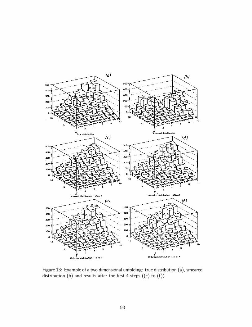
Figure 13: Example of a two dimensional unfolding: true distribution (a), smeareddistribution (b) and results after the first 4 steps ((c) to (f)).
93
may be made: “the iterative procedure is against the Bayesian spirit, sincethe same data are used many times for the same inference”. In principle theobjection is valid, but in practice this technique is a “trick” to give to theexperimental data a weight (an importance) larger than that of the priors. Amore rigorous procedure which took into account uncertainties and correla-tions of the initial distribution would have been much more complicated. Anattempt of this kind can be found in [22]. Examples of unfolding proceduresperformed with non-Bayesian methods are described in [20] and [21].
94

18 Conclusions
These notes have shown how it is possible to build a powerful theory of mea-surement uncertainty starting from a definition of probability which seems oflittle use at first sight, and from a formula that - some say - looks too trivialto be called a theorem.
The main advantages the Bayesian approach has over the others are (fur-ther to the non negligible fact that it is able to treat problems on which theothers fail):
• the recovery of the intuitive idea of probability as a valid concept fortreating scientific problems;
• the simplicity and naturalness of the basic tool;
• the capability of combining prior prejudices and experimental facts;
• the automatic updating property as soon as new facts are observed;
• the transparency of the method which allows the different assumptionson which the inference may depend to be checked and changed;
• the high degree of awareness that it gives to its user.
When employed on the problem of measurement errors, as a special ap-plication of conditional probabilities, it allows all possible sources of uncer-tainties to be treated in the most general way.
When the problems get complicated and the general method becomestoo heavy to handle, it is possible to use approximate methods based on thelinearization of the final probability density function to calculate the firstand second moments of the distribution. Although the formulae are exactlythose of the standard “error propagation”, the interpretation of the truevalue as a random variable simplifies the picture and allows easy inclusion ofuncertainties due to systematic effects.
Nevertheless there are some cases in which the linearization may causesevere problems, as shown in Section 14. In such cases one needs to go backto the general method or to apply other kinds of approximations which arenot just blind use of the covariance matrix.
The problem of unfolding dealt with in the last section should to be con-sidered a side remark with respect to the mainstream of the notes. It is infact a mixture of genuine Bayesian method (the basic formula), approxima-tions (covariance matrix evaluation) and ad hoc prescriptions of iteration andsmoothing, used to sidestep the formidable problem of seeking the generalsolution.
95

I would like to conclude with three quotations:
• “(. . . ) the best evaluation of the uncertainty (. . . ) must be given(. . . )The method stands, therefore, in contrast to certain older meth-ods that have the following two ideas in common:
– The first idea is that the uncertainty reported should be ’safe’or ’conservative’ (. . . ) In fact, because the evaluation of theuncertainty of a measurement result is problematic, it wasoften made deliberately large.
– The second idea is that the influences that give rise to un-certainty were always recognizable as either ’random’ or ’sys-tematic’ with the two being of different nature; (. . . )”
(ISO Guide[2])
• “Well, QED is very nice and impressive, but when everything isso neatly wrapped up in blue bows, with all experiments in exactagreement with each other and with the theory - that is when oneis learning absolutely nothing.”
“On the other hand, when experiments are in hopeless conflict -
or when the observations do not make sense according to conven-
tional ideas, or when none of the new models seems to work, in
short when the situation is an unholy mess - that is when one is
really making hidden progress and a breakthrough is just around
the corner!”
(R. Feynman, 1973 Hawaii Summer Institute, cited by D.Perkins at 1995 EPS Conference, Brussels)
• “Although this Guide provides a framework for assessing uncer-
tainty, it cannot substitute for critical thinking, intellectual hon-
esty, and professional skill. The evaluation of uncertainty is nei-
ther a routine task nor a purely mathematical one; it depends
on detailed knowledge of the nature of the measurand and of the
measurement. The quality and utility of the uncertainty quoted
for the result of a measurement therefore ultimately depend on
the understanding, critical analysis, and integrity of those who
contribute to the assignment of its value”. (ISO Guide[2])
96

Acknowledgements
It was a great pleasure to give the lectures on which these notes are based.I thank all the students for the active interests shown and for questions andcomments. Any further criticism on the text is welcome.
I have benefitted a lot from discussions on this subject with my Romeand DESY colleagues, expecially those of the ZEUS Collaboration. Specialacknowledgements go to Dr. Giovanna Jona-Lasinio and Prof. Romano Scoz-zafava of ‘’La Sapienza”, Dr. Fritz Frohner of FZK Karlsruhe (Germany),Prof. Klaus Weise of the PTB Braunschweig (Germany), and Prof. GunterZech of Siegen University (Germany) for clarifications on several aspects ofprobability and metrology. Finally, I would like to thank Dr. Fritz Frohner,Dr. Gerd Hartner of Toronto University (Canada), Dr. Jose Repond ofArgonne National Laboratory (USA) and Prof. Albrecht Wagner of DESY(Germany) for critical comments on the manuscript.
Bibliographic note
The state of the art of Bayesian theory is summarized in [7], where manyreferences can be found. A concise presentation of the basic principles caninstead been found in [24]. Text books that I have consulted are [4] and[6]. They contain many references too. As an introduction to subjectiveprobability de Finetti’s “Theory of probability”[5] is a must. I have foundthe reading of [25] particular stimulating and that of [26] very convincing(thanks expecially to the many examples and exercises). Unfortunately thesetwo books are only available in Italian for the moment.
Sections 6 and 7 can be reviewed in standard text books. I recommendthose familiar to you.
The applied part of these notes, i.e. after section 9, is, in a sense, “orig-inal”, as it has been derived autonomously and, in many cases, without theknowledge that the results have been known to experts for two centuries.Some of the examples of section 13 were worked out for these lectures. Thereferences in the applied part are given at the appropriate place in the text- only those actually used have been indicated. Of particular interest is theWeise and Woger theory of uncertainty[14], which differs from that of thesenotes because of the additional use of the Maximum Entropy Principle.
A consultation of the ISO Guide[2] is advised. Presently the BIPM recom-mendations are also followed by the american National Institute of Standardsand Technology (NIST), whose Guidelines[27] have the advantage, with re-spect to the ISO Guide, of being available on www too.
97

References
[1] DIN Deutsches Institut fur Normung, “Grunbegriffe der Messtechnick -Behandlung von Unsicherheiten bei der Auswertung von Messungen” (DIN1319 Teile 1-4), Beuth Verlag GmbH, Berlin, Germany, 1985. Only parts1-3 are published in English. An English translation of part 4 can be re-quested from the authors of [14]. Part 3 is going to be rewritten in orderto be made in agreement with [2] (private communication from K. Weise).
[2] International Organization for Standardization (ISO), “Guide to the ex-pression of uncertainty in measurement”, Geneva, Switzerland, 1993.
[3] H. Jeffreys, “Theory of probability”, Oxford University Press, 1961.
[4] R. L. Winkler, “An introduction to Bayesian inference and decision”, Holt,Rinehart and Winston, Inc., 1972.
[5] B. de Finetti, “Theory of probability”, J. Wiley & Sons, 1974.
[6] S. J. Press, “Bayesian statistics: principles, models, and applications”,John Wiley & Sons Ltd, 1989.
[7] J.M. Bernardo, A.F.M. Smith, “Bayesian theory”, John Wiley & Sons Ltd,Chichester, 1994.
[8] Particle Data Group, “Review of particle properties”, Phys. Rev. D, 50
(1994) 1173.
[9] New Scientist, April 28 1995, pag. 18 (“Gravitational constant is up in theair”). The data of Tab. 2 are from H. Meyer’s DESY seminar, June 281995.
[10] P.L. Gaison, “How experiments end”, The University of Chicago Press,1987.
[11] G. D’Agostini, “Limits on electron compositeness from the Bhabha scat-tering at PEP and PETRA”, Proceedings of the XXV th Rencontre deMoriond on “Z Physics”, Les Arcs (France), March 4-11, 1990, pag. 229(also DESY-90-093).
[12] A.K. Wroblewski, ”Arbitrariness in the development of physics”, after-dinner talk at the International Workshop on Deep Inelastic Scatteringand Related Subjects, Eilat, Israel, 6-11 February 1994, Ed. A. Levy (WorldScientific, 1994), pag. 478.
[13] E.T. Jaynes, “Information theory and statistical mechanics”, Phys. Rev.106 (1957) 620.
98
[14] K. Weise, W. Woger, “A Bayesian theory of measurement uncertainty”,Meas. Sci. Technol., 4 (1993) 1.
[15] International Organization for Standardization (ISO), “International vo-cabulary of basic and general terms in metrology”, Geneva, Switzerland,1993.
[16] G. D’Agostini, “On the use of the covariance matrix to fit correlated data”,Nucl. Instr. Meth. A346 (1994) 306.
[17] CELLO Collaboration, H.J. Behrend et al., “Determination of αs andsin2 θw from measurements of total hadronic cross section in e+e− annihi-lation”, Phys. Lett. 183B (1987) 400.
[18] S. Chiba and D.L. Smith, ”Impacts of data transformations on least-squaresolutions and their significance in data analysis and evaluation”, J. Nucl.Sc. Tech. 31 (1994) 770.
[19] M. L. Swartz, “Reevaluation of the hadronic contribution to α(M2Z)”,
SLAC-PUB-95-7001, September 1995, submitted to Phys. Rev. D.
[20] V. Blobel, Proceedings of the “1984 CERN School of Computing”,Aiguablava, Catalonia, Spain, 9-12 September 1984, Published by CERN,July 1985, pag. 88-127.
[21] G. Zech, “Comparing statistical data to Monte Carlo simulation - param-eter fitting and unfolding”, DESY 95-113, June 1995.
[22] K. Weise, “Matematical foundation of an analytical approach to bayesianMonte Carlo spectrum unfolding”, Physicalish Technische Bundesanstalt,Braunschweig, BTB-N-24, July 1995.
[23] G. D’Agostini, “A multidimensional unfolding method based on Bayes’ the-orem”, Nucl. Instr. Meth. A362 (1995) 487.
[24] C. Howson and P. Urbach, “Bayesian reasoning in science”, Nature, Vol.350, 4 April 1991, pag. 371.
[25] B. de Finetti, “Filosofia della probabilita”, il Saggiatore, 1995.
[26] R. Scozzafava, “La probabilita soggettiva e le sue applicazioni”, Masson,editoriale Veschi, Roma, 1993.
[27] B.N. Taylor and C.E. Kuyatt, “Guidelines for evaluating and expressinguncertainty of NIST measurement results”, NIST Technical Note 1297,September 1994;(www: http://physics.nist.gov/Pubs/guidelines/outline.html).
99