Probability and Measure

Stefan Grosskinsky

Cambridge, Michaelmas 2006

These notes and other information about the course are available onwww.statslab.cam.ac.uk/ ∼stefan/teaching/probmeas.html

The text is based on – and partially copied from – notes on the same course by James Nor-ris, Alan Stacey and Geoffrey Grimmett.

Contents

Introduction 3

1 Set systems and measures 51.1 Set systems. . . . . . . . . . . . . . . . . . . . . . . . . . . . . . . . . . . . 51.2 Measures . . . . . . . . . . . . . . . . . . . . . . . . . . . . . . . . . . . . . 61.3 Extension and uniqueness. . . . . . . . . . . . . . . . . . . . . . . . . . . . . 81.4 Lebesgue(-Stieltjes) measure. . . . . . . . . . . . . . . . . . . . . . . . . . . 101.5 Independence and Borel-Cantelli lemmas. . . . . . . . . . . . . . . . . . . . 13

2 Measurable Functions and Random Variables 152.1 Measurable Functions. . . . . . . . . . . . . . . . . . . . . . . . . . . . . . .152.2 Random Variables. . . . . . . . . . . . . . . . . . . . . . . . . . . . . . . . .172.3 Convergence of measurable functions. . . . . . . . . . . . . . . . . . . . . . 19

3 Integration 223.1 Definition and basic properties. . . . . . . . . . . . . . . . . . . . . . . . . . 223.2 Integrals and limits. . . . . . . . . . . . . . . . . . . . . . . . . . . . . . . .253.3 Integration inR and differentiation. . . . . . . . . . . . . . . . . . . . . . . . 283.4 Product measure and Fubini’s theorem. . . . . . . . . . . . . . . . . . . . . . 30

4 Lp-spaces 334.1 Norms and inequalities. . . . . . . . . . . . . . . . . . . . . . . . . . . . . .334.2 L2 as a Hilbert space. . . . . . . . . . . . . . . . . . . . . . . . . . . . . . .364.3 Convergence inL1 . . . . . . . . . . . . . . . . . . . . . . . . . . . . . . . .39

1

5 Characteristic functions and Gaussian random variables 415.1 Definitions. . . . . . . . . . . . . . . . . . . . . . . . . . . . . . . . . . . . .415.2 Properties of characteristic functions. . . . . . . . . . . . . . . . . . . . . . . 425.3 Gaussian random variables. . . . . . . . . . . . . . . . . . . . . . . . . . . . 43

6 Ergodic theory and sums of random variables 466.1 Motivation. . . . . . . . . . . . . . . . . . . . . . . . . . . . . . . . . . . . .466.2 Measure-preserving transformations. . . . . . . . . . . . . . . . . . . . . . . 466.3 Ergodic Theorems. . . . . . . . . . . . . . . . . . . . . . . . . . . . . . . . .496.4 Limit theorems for sums of random variables. . . . . . . . . . . . . . . . . . 51

Appendix A – Example sheets 53A.1 Example sheet 1 – Set systems and measures. . . . . . . . . . . . . . . . . . 53A.2 Example sheet 2 – Measurable functions and integration. . . . . . . . . . . . 55A.3 Example sheet 3 – Convergence, Fubini,Lp-spaces . . . . . . . . . . . . . . . 57A.4 Example sheet 4 – Characteristic functions, Gaussian rv’s, ergodic theory. . . 59

Appendix B – Hand-outs 61B.1 Hand-out 1 – Proof of Caratheodory’s extension theorem. . . . . . . . . . . . 61B.2 Hand-out 2 – Convergence of random variables. . . . . . . . . . . . . . . . . 63B.3 Hand-out 3 – Connection between Lebesgue and Riemann integration. . . . . 65B.4 Hand-out 4 – Ergodic theorems. . . . . . . . . . . . . . . . . . . . . . . . . . 66

2

Introduction

Motivation from two perspectives:

1. ProbabilityLet

(Ω,P(Ω), P

)be a probability space, whereΩ is a set,P(Ω) the set of events (power set in

this case) andP : P(Ω) → [0, 1] is the probability measure.If Ω is countable then we have for everyA ∈ P(Ω)

P(A) =∑ω∈A

P(ω

).

So calculating probabilities just involves (possibly infinite) sums.If Ω = [0, 1] andP is the uniform probability measure on[0, 1] then for everyω ∈ Ω it isP(ω) = 0. So

1 = P([0, 1]

)6= “

∑w∈[0,1]

P(ω

)“.

2. Integration (Analysis)WhenP can be described by a densityρ : Ω → [0,∞) we can handle the situation via

P(A) =∫

Aρ(x) dx =

∫Ω1A(x) ρ(x) dx , (∗)

where1A is the indicator function of the setA. In the example aboveρ(x) ≡ 1 and this leadsto P

([a, b]

)=

∫ 10 1[a,b](x) dx =

∫ ba dx = b− a.

In general this approach only makes sense if the integral(∗) exists. Using the theory ofRiemann-integration we are fine as long asA is a finite union or intersection of intervals andρ(x) is e.g. continuous. But e.g. forA = [0, 1] ∩ Q, the Riemann-integral

∫ 10 1A(x) dx is not

defined, although the probability for this event is intuitively0.Moreover, sinceA is countable, it can be written asA =

an : n ∈ N

. Define

fn := 1a1,...,an with fn → 1A for n → ∞. For everyn, fn is Riemann-integrable and∫ 10 fn(x) dx = 0. So it should be the case that

limn→∞

∫ 1

0fn(x) dx = 0 ?=

∫ 1

01A(x) dx ,

but the latter integral is not defined. Thus the concept of Riemann-integrals is not satisfac-tory for two reasons: The set of Riemann-integrable functions is not closed, and there are “toomany” functions which are not Riemann-integrable.

Goals of this course

• Generalisation of Riemann-integration to Lebesgue-integration using measure theory,involving a precise treatment of setsA and functionsρ for which (∗) is defined

• Using measure theory as the basis of advanced probability and discussing applicationsin that area

3

Official scheduleMeasure spaces,σ-algebras,π-systems and uniqueness of extension, statement * and proof *of Caratheodory’s extension theorem. Construction of Lebesgue measure onR. The Borelσ-algebra ofR. Existence of non-measurable subsets ofR. Lebesgue-Stieltjes measures andprobability distribution functions. Independence of events, independence ofσ-algebras. TheBorel-Cantelli lemmas. Kolmogorov’s zero-one law. [6]Measurable functions, random variables, independence of random variables. Construction ofthe integral, expectation. Convergence in measure and convergence almost everywhere. Fa-tou’s lemma, monotone and dominated convergence, differentiation under the integral sign.Discussion of product measure and statement of Fubini s theorem. [6]Chebyshev s inequality, tail estimates. Jensen’s inequality. Completeness ofLp for 1 ≤ p ≤ ∞. The Holder and Minkowski inequalities, uniform integrability. [4]L2 as a Hilbert space. Orthogonal projection, relation with elementary conditional probability.Variance and covariance. Gaussian random variables, the multivariate normal distribution. [2]The strong law of large numbers, proof for independent random variables with bounded fourthmoments. Measure preserving transformations, Bernoulli shifts. Statements * and proofs *of maximal ergodic theorem and Birkhoff s almost everywhere ergodic theorem, proof of thestrong law. [4]The Fourier transform of a finite measure, characteristic functions, uniqueness and inversion.Weak convergence, statement of Levy’s convergence theorem for characteristic functions. Thecentral limit theorem. [2]

Appropriate booksP. Billingsley,Probability and Measure. Wiley 1995 (hardback).R.M. Dudley,Real Analysis and Probability. CUP 2002 (paperback).R.L.Schilling,Measures, Integrals and Martingales. CUP 2005 (paperback).R.T. Durrett,Probability: Theory and Examples. Wadsworth a. Brooks/Cole 1991 (hardback).D. Williams, Probability with Martingales. CUP (paperback).

From the point of view of analysis, the first chapters of this book might be interesting:S. Kantorovitz,Introduction to Modern Analysis. Oxford 2003 (hardback).

Non-examinable material

• proof of Caratheodory’s extension theorem on hand-out 1

• part (a) of the proof of Skorohod’s representation theorem on hand-out 2

• connection between Lebesgue and Riemann integration on hand-out 3

• Proof of the maximal ergodic lemma and Birkhoff’s almost everywhere ergodic theoremon hand-out 4 and in Section 6

4

1 Set systems and measures

Let E be an arbitrary set andE ⊆ P(E) a set of subsets. To define a measureµ : E → [0,∞)(see section 1.2) we first need to identify a proper domain of definition.

1.1 Set systems

Definition 1.1. Say thatE is aring, if for all A,B ∈ E(i) ∅ ∈ E (ii) B \A ∈ E (iii) A ∪B ∈ E .

Say thatE is analgebra(or field), if for all A,B ∈ E(i) ∅ ∈ E (ii) Ac = E \A ∈ E (iii) A ∪B ∈ E .

Say thatE is aσ-algebra(or σ-field), if for all A andA1, A2, . . . ∈ E

(i) ∅ ∈ E (ii) Ac ∈ E (iii)⋃n∈N

An ∈ E .

Properties. (i) A (σ-)algebra is closed under (countably) finitely many set operations, since

A ∩B =(Ac ∪Bc

)c ∈ E ,⋂n∈N

An =( ⋃

n∈NAc

n

)c, 1

A \B = A ∩Bc ∈ E , A4B = (A \B) ∪ (B \A) ∈ E .

(ii) Thus: E is aσ-algebra ⇒ E is an algebra ⇒ E is a ringIn general the inverse statementss are false, but in special cases they hold:

⇐ (if E is finite) ⇐ (if E ∈ E)

Examples.(i) P(E) and∅, E are the largest and smallestσ-algebras onE, respectively

(ii) E = R,R =⋃n

i=1(ai, bi] : ai < bi, i = 1, . . . , n, n ∈ N0

is the

ring of half-open intervals (∅ is given by the empty intersectionn = 0).R is an algebra if we allow for infinite intervals and identifyR = (−∞,∞].

(iii) Beware:⋃∞

i=1(ai, bi] : ai, bi ∈ [−∞,∞], ai < bi, i ∈ N,

is anot aσ-algebra.

(see problem 1.9(a))

Lemma 1.1. LetEi : i ∈ I

be a (possibly uncountable) collection ofσ-algebras. Then⋂

i∈I Ei is aσ-algebra, whereas⋃

i∈I Ei in general is not.

Proof. Let E =⋂

i∈I Ei. We check (i) to (iii) in the above definition:(i) Since∅ ∈ Ei for all i ∈ I, ∅ ∈ E . (ii) Since for allA ∈ E , Ac ∈ Ei for all i ∈ I, Ac ∈ E .(iii) Let A1, A2, . . . ∈ E . ThenAk ∈ Ei for all k ∈ N andi ∈ I, hence

⋃n∈N An ∈ Ei for each

i ∈ I and so⋃

n∈N An ∈ E . For the second part see problem 1.1 (c). 2

Definition 1.2. LetA ⊆ P(E). Then theσ-algebra generated byA is

σ(A) :=⋂E⊃A

E σ−alg.

E , the smallestσ-algebra containingA.

1as long as (ii) is fulfilled “∪” and “∩” are equivalent

5

Remarks. (i) If E is aσ-algebra, thenσ(E) = E .

(ii) LetA1, A2 ⊆ P(E) with A1 ⊆ A2. Thenσ(A1) ⊆ σ(A2).

Examples. (i) Let ∅ 6= A ( E. Thenσ(A

)= ∅, E, A,Ac.

(ii) If E is aσ-algebra, so isA ∩ E = A ∩ B : B ∈ E for eachA ∈ E, called thetraceσ-algebraof A.

The next example is so important, that we spend an extra definition.

Definition 1.3. Let (E, τ) be atopological spacewith topologyτ ⊆ P(E) (set of open sets)2.Thenσ(τ) is called theBorel σ-algebraof E, denoted byB(E). A ∈ B(E) is called aBorelset. One usually denotesB(R) = B.

Lemma 1.2. Let E = R, R the ring of half-open intervals andI =(a, b] : a < b

the set of all half-open intervals. Thenσ(R) = σ(I) = B.

Proof. (i) I ⊆ R ⇒ σ(I) ⊆ σ(R). On the other hand, eachA ∈ R can be written asA =

⋃ni=1(ai, bi] ∈ σ(I). ThusR ⊆ σ(I) ⇒ σ(R) ⊆ σ(I).

(ii) EachA ∈ I can be written asA = (a, b] =⋂∞

n=1(a, b + 1n) ∈ B ⇒ σ(I) ⊆ B.

Let A ⊆ R be open, i.e.∀x∈A ∃ εx>0 : (x− εx, x + εx) ⊆ A. Thus

∀ x ∈ A ∃ ax, bx ∈ Q : x ⊆ (ax, bx] ⊆ A .

ThenA =⋃

x∈A(ax, bx] which is a countable union, sinceax, bx ∈ Q.ThusA ∈ σ(I) ⇒ B ⊆ σ(I). 2

Remarks. (i) The Borelσ-algebra onA ⊆ R isB(A) = A ∩ B (traceσ-algebra ofA).

(ii) Analogously,B(Rd) is generated byId = d∏

i=1

(ai, bi] : ai < bi, 1 = 1, . . . , d

and

this is consistent withd = 1 in the sense thatB(Rd) = Bd.

Definition 1.4. Let E ⊆ P(E) be aσ-algebra. The pair(E, E) is a measurable spaceandelements ofE aremeasurable sets.

If E is finite or countably infinite, one usually takesE = P(E) as relevantσ-algebra.

1.2 Measures

Definition 1.5. Let E be a ring onE. A set functionis anyµ : E → [0,∞] with µ(∅) = 0.

• µ is calledadditiveif for all A,B ∈ E with A ∩B = ∅: µ(A ∪B) = µ(A) + µ(B).

• µ is called countably additive(or σ-additive) if for all sequences(An)n∈N with

Ai ∩Aj = ∅ for i 6= j and⋃

n∈NAn ∈ E : µ

( ⋃

n∈NAn

)=

∑n∈N

µ(An).

2Having a direct definition of open sets forE = Rd, there is also an axiomatic definition of a topology, namely(i) ∅ ∈ τ andE ∈ τ (ii) ∀A, B ∈ τ : A ∩B ∈ τ (iii)

⋃i∈I Ai ∈ τ , givenAi ∈ τ for all i ∈ I

6

Note. µ countably additive⇒ µ additive[A1 = A,A2 = B,A3 = A4 = . . . = ∅

]Definition 1.6. Let (E, E) be a measurable space. A countably additive set functionµ : E → [0,∞] is called ameasure, the triple(E, E , µ) is calledmeasure space.If µ(E) < ∞, µ is calledfinite. If µ(E) = 1, µ is a probability measureand(E, E , µ) is aprobability space. If E is a topological space andE = B(E), thenµ is calledBorel measure.

Basic properties.Let (E, E , µ) be a measure space.

(i) µ is non-decreasing: For allA,B ∈ E , A ⊆ B it is µ(B) = µ(B \A) + µ(A) ≥ µ(A).(Note: The versionµ(B \A) = µ(B)− µ(A) only makes sense ifµ(A) < ∞).

(ii) µ is subadditive: For allA,B ∈ E , µ(A ∪B) ≤ µ(A) + µ(B) since

µ(A) + µ(B) = µ(A \B) + µ(A ∩B) + µ(B \A)︸ ︷︷ ︸=µ(A∪B)

+µ(A ∩B) =

= µ(A ∪B) + µ(A ∩B) ≥ µ(A ∪B) .

(Again: µ(A ∪B) = µ(A) + µ(B)− µ(A ∩B) only if µ(A ∩B) < ∞.)

(iii) µ is alsocountably subadditive(see problem 1.6 (b)).

(iv) Let E1 ⊆ E2 beσ-algebras. Ifµ is a measure onE2, then it is also onE1.

(v) ForA ∈ E therestrictionµ|A = µ(. ∩A) is a measure on(E, E).

Remark. These properties also hold for countably additive set functions (calledpre-measures)on a ring , (i) and (ii) also for additive set functions on a ring.

Examples. (i) For everyx ∈ E, theDirac measureis given by δx(A) =

1 , x ∈ A0 , x 6∈ A

.

(ii) Discrete measure theory:Let E be countable. Every measureµ on (E,P(E)) can be characterized by amassfunctionm : E → [0,∞],

µ =∑x∈E

m(x) δx or equivalently ∀ A ⊆ E : µ(A) =∑x∈A

µ(x

)=

∑x∈A

m(x) .

If m(x) ≡ 1 for all x ∈ E, µ is calledcounting measure.

(iii) Let E = R andR be the ring of half-open intervals. ForA ∈ R write A =⋃ n

i=1(ai, bi]with disjoint intervals,n ∈ N0. We call this astandard representationof A. Althoughit is not unique, the set functionµ : R → [0,∞] with µ(A) :=

∑ni=1(bi − ai) is

independent of the particular representation and thus well defined.Further,µ is additive andtranslation invariant, i.e.∀x∈R : µ(A + x) = µ(A), whereA + x := x + y : y ∈ A. The key question is:

Canµ be extended to a measure onB = σ(R)?

7

In order to attack this question in the next subsection, it is useful to introduce the followingproperty of set functions.

Definition 1.7. Let E be a ring onE andµ : E → [0,∞] an additive set function.µ iscontinuous atA ∈ E , if

(i) µ is continuous from below:given anyA1 ⊆ A2 ⊆ A3 ⊆ . . . in E with

⋃n∈N

An = A ∈ E (An A),

then limn→∞

µ(An) = µ(A)

(ii) µ is continuous from above:given anyA1 ⊇ A2 ⊇ A3 ⊇ . . . in E with

⋂n∈N

An = A ∈ E (An A) and

µ(An) < ∞ for somen ∈ N, then limn→∞

µ(An) = µ(A)

Lemma 1.3. LetE be a ring onE andµ : E → [0,∞] an additive set function. Then:

(i) µ is countably additive ⇒ µ is continuous at allA ∈ E

(ii) µ is continuous from below at allA ∈ E ⇒ µ is countably additive

(iii) µ is cont. from above at∅ andµ(A) < ∞ for all A ∈ E ⇒ µ is countably additive

Remark. The conditionµ(An) < ∞ for somen ∈ N in (ii) of the definition is necessary formeasures to be continuous. Consider e.g.E = N, Ak = k, k + 1, . . . andµ the countingmeasure. Thenµ(Ak) = ∞ for all k ∈ N, butµ(A) = µ(∅) = 0.

Proof. (i) GivenAn A in E , thenA = (A1 \A0) ∪ (A2 \A1) ∪ (A3 \A2) ∪ . . . (A0 = ∅)

⇒ µ(A) =∞∑

n=0

µ(An+1 \An) = limm→∞

µ( m−1⋃

n=0

(An+1 \An))

= limm→∞

µ(Am) .

GivenAn A in E andµ(Am) < ∞ for somem ∈ N. LetBn := Am \An for n ≥ m. ThenBn (Am \A) for n →∞ and thus, following the above,

µ(Am)− µ(An) = µ(Bn) n→∞−→ µ(Am \A) = µ(Am)− µ(A) .

Sinceµ(Am) < ∞ this implies limn→∞

µ(An) = µ(A).(ii) see problem 1.6 (a)(iii) analogous to (i) and (ii) 2

1.3 Extension and uniqueness

Theorem 1.4. Caratheodory’s extension theoremLet E be a ring onE and µ : E → [0,∞] be a countably additive set function. Then thereexists a measureµ′ on

(E, σ(E)

)such that µ′(A) = µ(A) for all A ∈ E .

8

Proof. The proof is not examinable and is given on Hand-out 1 in the appendix.

To formulate a result on uniqueness two further notions are useful.

Definition 1.8. Let E be a set.E ⊆ P(E) is called aπ-systemif ∀A,B ∈ A : A∩B ∈ A .E is called ad-systemif

(i) E ∈ E , (ii) ∀ A,B ∈ E , A ⊆ B : B \A ∈ E ,

(iii) ∀ A1, A2, . . . ∈ E : A1 ⊆ A2 ⊆ . . . ⇒⋃n∈N

An ∈ E .

Remarks.

(i) The setI ∪ ∅ =(a, b] : a < b

∪ ∅ is aπ-system onR and we have shown in

Lemma 1.2 thatσ(I) = B.

(ii) E is aσ-algebra⇔ E is aπ- and ad-system (see problem 1.8 (a)).

Lemma 1.5. Dynkin’sπ-system lemmaLetE be aπ-system. Then for anyd-systemD ⊇ E it is D ⊇ σ(E).

Proof. The intersection∆(E) =⋂D⊃E D of all d-systems containingE is itself ad-system.

We shall show that∆(E) is also aπ-system. Then it is also aσ-algebra and for anyd-systemD ⊇ E we haveD ⊇ ∆(E) ⊇ σ(E), thus proving the lemma. Consider

D′ =B ∈ ∆(E) : B ∩A ∈ ∆(E) for all A ∈ E

⊆ ∆(E) .

ThenE ⊆ D′ becauseE is aπ-system. We check thatD′ is ad-system, and henceD′ = ∆(E).(i) clearlyE ∈ D′;(ii) supposeB1, B2 ∈ D′ with B1 ⊆ B2, then forA ∈ E we have

(B2 \B1) ∩A = (B2 ∩A) \ (B1 ∩A) ∈ ∆(E) ,

because∆(E) is ad-system, soB2 \B1 ∈ D′;(iii) finally, if Bn ∈ D′ andBn B, then forA ∈ E

Bn ∩A B ∩A ∈ ∆(E) ⇒ B ∈ D′ .

Now consider

D′′ =B ∈ ∆(E) : B ∩A ∈ ∆(E) for all A ∈ ∆(E)

⊆ D′ .

ThenE ⊆ D′′ becauseD′ = ∆(E). We can check thatD′′ is ad-system, just as we did forD′.HenceD′′ = ∆(E) which shows that∆(E) is aπ-system. 2

Theorem 1.6. Uniqueness of extensionLet E ⊆ P(E) be a π-system. Suppose thatµ1, µ2 are measures onσ(E) withµ1(E) = µ2(E) < ∞. If µ1 = µ2 onE thenµ1 = µ2 onσ(E).Equivalently, ifµ(E) < ∞ the measureµ onσ(E) is uniquely determined by its values on theπ-systemE .

9

Proof. ConsiderD =A ∈ σ(E) : µ1(A) = µ2(A)

⊆ σ(E). By hypothesis,E ∈ D.

ForA,B ∈ D with A ⊆ B we have

µ1(B \A) = µ1(B)− µ1(A) = µ2(B)− µ2(A) = µ2(B \A) < ∞ ,

thus alsoB \A ∈ D. If An ∈ D, n ∈ N, with An A, then

µ1(A) = limn→∞

µ1(An) = limn→∞

µ2(An) = µ2(A) ⇒ A ∈ D .

ThusD ⊆ σ(E) is ad-system containing theπ-systemE , soD = σ(E) by Dynkin’s lemma.2

These theorems provide general tools for the construction and characterisation of measuresand will be applied in a specific context in the next subsection.

1.4 Lebesgue(-Stieltjes) measure

Theorem 1.7. There exists a unique Borel measureµ on (R,B) such that

µ((a, b]

)= b− a , for all a, b ∈ R with a < b.

The measureµ is calledLebesgue measureonR.

Proof. (Existence) LetR be the ring of half-open intervals. Consider the set functionµ(A) =

∑ni=1(bi − ai), whereA =

⋃ n

i=1(ai, bi], n ∈ N0. We aim to show thatµ is countablyadditive onR, which then proves existence by Caratheodory’s extension theorem.Sinceµ(A) < ∞ for all A ∈ R, by Lemma 1.3 (iii) it suffices to show thatµ is continuousfrom above at∅. Suppose not. Then there existsε > 0 andAn ∅ with µ(An) ≥ 2ε for all n.For eachn we can findCn ∈ R with Cn ⊆ An andµ(An \Cn) ≤ ε2−n (see problem 1.9 (b)).Then

µ(An \ (C1 ∩ . . . ∩ Cn)

)≤

n∑k=1

µ(An \ Ck) ≤n∑

k=1

µ(Ak \ Ck) ≤∞∑

k=1

ε2−k = ε ,

and sinceµ(An) ≥ 2ε we haveµ(C1∩ . . .∩Cn) ≥ ε and in particularC1∩ . . .∩Cn 6= ∅. ThusKn = C1 ∩ . . . ∩ Cn, n ∈ N is a monotone sequence of compact non-empty sets. Thus thereexists a sequence(xn)n∈N with xn ∈ Kn which has at least one accumulation pointx∗, since allxn ∈ K1 which is compact. SinceKn , x∗ ∈

⋂n∈N Kn. Thus∅ 6=

⋂n∈N Kn ⊆

⋂n∈N An

which is a contradiction toAn ∅.(Uniqueness) For eachn ∈ Z define

µn(A) := µ((n, n + 1] ∩A

)for all A ∈ B .

Thenµn is a probability measure on(R,B), so, by Theorem 1.6,µn is uniquely determindedby its values on theπ-systemI generatingB. Sinceµ(A) =

∑n∈Z µn(A) it follows thatµ is

also uniquely determined. 2

Definition 1.9. A ⊆ R is callednull if A ⊆ B ∈ B with µ(B) = 0. Denote byN theset of all null sets. ThenL =

B ∪N : b ∈ B, N ∈ N

is thecompletionof B and is called

Lebesgueσ-algebra. The sets inL are calledLebesgue-measurable setsor Lebesgue sets.

10

Remark. The Lebesgue measureµ can be extended toL via (see problem 1.10)

λ(B ∪N) := µ(B) for all B ∈ B, N ∈ N .

In some books onlyλ is calledLebesgue measure. This makes sense e.g. in analysis, whereone usually works with a fixed measure space(R,L, λ).

Theorem 1.8. B ( L ( P(R). Moreover3

card(B) = card(R) = c whereas card(L) = card(P(R)

)= 2c .

Proof. (i) According to problem 1.4,B is separable, i.e. generated by a countable set sys-tem E . Thuscard(B) ≤ card

(P(E)

)= c. On the other hand,x ∈ B for all x ∈ R

and thuscard(B) = c. With problem 1.10 the Cantor setC ⊆ R is uncountable and thuscard(C) = c. Since alsoµ(C) = 0, with Definition 1.9 we haveP(C) ⊆ L and thuscard(L) = card

(P(R)

)= 2c > c.

(ii) Using the axiom of choice we construct a subset ofU = [0, 1] which is not inL:Define the equivalence relation∼ onU by x ∼ y if x− y ∈ Q.Write Ei : i ∈ I for the equivalence classes of∼ and let R = ei : i ∈ I be acollection of representativesei ∈ Ei, chosen by the axiom of choice. ThenU can be partitioned

U =⋃

i∈I

Ei =⋃

i∈I

⋃

q∈Q∩[0,1)

(ei + q) =⋃

q∈Q∩[0,1)

⋃

i∈I

(ei + q)︸ ︷︷ ︸=R+q

=⋃

q∈Q∩[0,1)

(R + q) ,

where+ is to be understood modulo1. SupposeR ∈ L, thenR+q ∈ L andλ(R) = λ(R+q)for all q ∈ Q by translation invariance ofλ. But by countable additivity ofλ this means∑

q∈Q∩[0,1)

λ(R) = λ(U) = 1 ,

which leads to a contradiction for eitherλ(R) = 0 or λ(R) > 0. ThusR 6∈ L. 2

Remarks. (i) Every set of positive measure has non-measurable subsets and, moreover:

P(A) ⊆ L ⇔ λ(A) = 0 .

(ii) There exists no translation invariant, countably additive set function onP(R) withµ([0, 1]

)∈ (0,∞).

Definition 1.10. F : R → R is calleddistribution functionif

(i) F is non-decreasing (ii) F is right-continuous, i.e.limxx0

F (x) = F (x0) .

F is aprobability distribution functionif in addition

(iii) limx→∞

F (x) = 1 , limx→−∞

F (x) = 0 .

3Notation: Thecardinality of a countable set (such asN or Q) is ℵ0, for a continuous set (such asP(N), R orthe Cantor setC) it is 2ℵ0 = c. For power sets of the latter we just writecard

(P(R)

)= 2c.

11

Proposition 1.9. Letµ be a Radon measure4 on (R,B). Then for everyr ∈ R

Fr(x) :=

µ((r, x]

), x > r

−µ((x, r]

), x ≤ r

(in particular Fr(r) = −µ(∅) = 0

)is a distriburion function with µ

((a, b]

)= Fr(b)− Fr(a), a < b .

AlsoFr + C is a distribution function with that property for allC ∈ R.TheFr differ only in an additive constant, namelyFr(x) = F0(x)− F0(r) for all r ∈ R.

Proof. Fr by monotonicity ofµ andµ((a, b]

)= Fr(b) − Fr(a) for b > a by defini-

tion. Forxn x > r it is Fr(xn) = µ((r, xn]

) µ

((r, x]

)= Fr(x) by continuity of

measures. Forxn r we have(r, xn] ∅ such that Fr(xn) µ(∅) = 0 = Fr(r) .TheFr differ only in a constant, since for allx > r

µ(∅) = µ((r, x]

)− µ

((r, x]

)= F0(x)− F0(r)− Fr(x) + Fr(r) = 0 ,

andFr(r) = 0 = F0(r)− F0(r) . Both statements follow analogously forx < 0. 2

Remarks. (i) The distribution functions for the Lebesgue measure areFr(x) = x + r, r ∈ R.

(ii) Note that forxn x we have(xn, x] x 6= ∅, so thatFr as defined in Proposition1.9 is in general not left-continuous.

(iii) If µ is a probability measure one usually uses thecumulative distribution function

CDFµ(x) := F−∞(x) = µ((−∞, x]

).

E.g. for the Dirac measureδa concentrated ina ∈ R, CDFδa(x) =

0 , x < a1 , x ≥ a

.

On the other hand, a distribution function uniquely determines a Radon measure.

Theorem 1.10. Let F : R → R be a distribution function. Then there exists a unique RadonmeasureµF on (R,B), such that

µF

((a, b]

)= F (b)− F (a) for all a < b .

The measureµF is called theLebesgue-Stieltjes measureof F .

Proof. As for Lebesgue measure, the set functionµF is well defined on the ringR via

µ(A) :=n∑

i=1

(F (bi)− F (ai)

)where A =

n⋃

i=1

(ai, bi] .

The proof is then the same as that of Theorem 1.7 for Lebesgue measure. 2

Remark. Analogous to Definition 1.9,B can also be completed with respect to the Lebesgue-Stieltjes measureµF . However, the completionLµF depends on the measureµF . AlthoughLis much larger thanB (see Theorem 1.8), it is therefore preferable to work with the measurespace(R,B), since it is defined independent of the measure and allµF will have the samedomain of definition.

4i.e.µ(K) < ∞ for K ∈ B compact

12

1.5 Independence and Borel-Cantelli lemmas

Let (E, E , P) be a probability space. It provides a model for an experiment whose outcomeis random.E describes the set of possible outcomes,E the set of events (observable sets ofoutcomes) andP(A) is the probability of an eventA ∈ E .

Definition 1.11. The events(Ai)i∈I , Ai ∈ E , are said to beindependentif

P( ⋂

i∈J

Ai

)=

∏i∈J

P(Ai) for all finite, nonemptyJ ⊆ I .

Theσ-algebras(Ei)i∈I , Ei ⊆ E are said to beindependentif the events(Ai)i∈I are independentfor any choiceAi ∈ Ei.

A useful way to establish independence of twoσ-algebra is given below.

Theorem 1.11. LetE1, E2 ⊆ E beπ-systems and suppose that

P(A1 ∩A2) = P(A1) P(A2) wheneverA1 ∈ E1, A2 ∈ E2 .

Thenσ(E1) andσ(E2) are independent.

Proof. Fix A1 ∈ E1 and define the measuresµ, ν by

µ(A) = P(A1 ∩A) , ν(A) = P(A1) P(A) for all A ∈ E .

µ andν agree on theπ-systemE2 with µ(E) = ν(E) = P(A1) < ∞. So, by uniqueness ofextension (Theorem 1.6), for allA1 ∈ E1 andA2 ∈ σ(E2)

P(A1 ∩A2) = µ(A2) = ν(A2) = P(A1) P(A2) .

Now fix A2 ∈ σ(E2) and repeat the same argument with

µ′(A) := P(A ∩A2) , ν ′(A) := P(A) P(A2)

to show that for allA1 ∈ σ(E1) we have P(A1 ∩A2) = P(A1) P(A2). 2

Remark. In particular, theσ-algebrasσ(A1

)andσ

(A2

)generated by single events are

independent if and only ifA1 andA2 are independent.

Background. Let (an)n∈N be a sequence inR. Then limn→∞

an does not necessarily exist,

e.g. foran = (−1)n. To nevertheless study asymptotic properties of(an)n∈N consider

an = infk≥n

ak and an = supk≥n

ak .

Thenan andan are monotone and both have limits inR = R ∪ −∞,+∞. Define

lim infn→∞

an := limn→∞

infk≥n

ak and lim supn→∞

an := limn→∞

supk≥n

ak ,

which are equal to the smallest and largest accumulation point of(an)n∈N, respectively. Ingeneral lim inf

n→∞an ≤ lim sup

n→∞an since am ≤ am∨n ≤ an for all m,n ∈ N. They may be

13

different, as e.g. lim infn→∞

(−1)n = −1 < 1 = lim supn→∞

(−1)n . Both are equal if and only if

limn→∞

an exists. Note that a sequence may have much more than two accumulation points, e.g.

for an = sinn the set of accumulation points is[−1, 1], lim infn→∞

an = −1 andlim supn→∞

an = 1.

We use the same concept for a sequence(An)n∈N of subsets of a setE. Note that⋂

k≥n Ak and

⋃k≥n Ak are monotone inn.

Definition 1.12. Let (An)n∈N be a sequence of sets inE. Then define the sets

lim infn→∞

An :=⋃n∈N

⋂k≥n

Ak and lim supn→∞

An :=⋂n∈N

⋃k≥n

Ak .

Remark. This definition can be interpreted as

lim infn→∞

An =x : ∃n∈N ∀k≥n x ∈ Ak

=

x : x ∈ An for all but finitely manyn

lim sup

n→∞An =

x : ∀n∈N ∃k≥n x ∈ Ak

=

x : x ∈ An for infinitely manyn

.

One also writeslim infn→∞

An =’An ev.’ (eventually) andlim supn→∞

An =’An i.o.’ (infinitely often).

Properties. (i) Let E be aσ-algebra. IfAn ∈ E for all n ∈ N thenlim infn→∞

An, lim supn→∞

An ∈ E .

(ii) lim infn→∞

An ⊆ lim supn→∞

An since x ∈ An eventually⇒ x ∈ An infinitely often

(iii)(lim sup

n→∞An

)c = lim infn→∞

Acn since x ∈ An finitely often⇔ x ∈ Ac

n eventually.

Lemma 1.12. First Borel-Cantelli lemmaLet (E, E , µ) be a measure space and(An)n∈N a sequence of sets inE .

If∑n∈N

µ(An) < ∞ then µ(An i.o.) = 0 .

Proof. µ(An i.o.) = µ( ⋂

n∈N

⋃k≥n

Ak

)≤ µ

( ⋃k≥n

Ak

)≤

∑k≥n

µ(Ak) → 0 for n →∞. 2

Lemma 1.13. Second Borel-Cantelli lemmaLet (E, E , P) be a probability space and suppose that(An)n∈N are independent.

If∑n∈N

P(An) = ∞ , then P(An i.o.) = 1 .

Proof. We use the inequality1 − a ≤ e−a. With (An)n∈N also (Acn)n∈N are independent

(see problem 1.11). Then we have for alln ∈ N

P( ⋂

k≥n

Ack

)=

∏k≥n

(1− P(Ak)

)≤ exp

[−

∑k≥n

P(Ak)]

= 0 .

Hence P(An i.o.) = 1− P(

lim infn→∞

Acn

)= 1− P

( ⋃n∈N

⋂k≥n

Ack

)= 1 . 2

14

2 Measurable Functions and Random Variables

2.1 Measurable Functions

Definition 2.1. Let (E, E) and(F,F) be measurable spaces. A functionf : E → F is calledmeasurable (with respect toE andF) or E/F-measurableif

∀ A ∈ F : f−1(A) =x ∈ E : f(x) ∈ A

∈ E

(short:f−1(F) ⊆ E

).

Often (F,F) = (R,B) or (R,B) with the extended real lineR = R ∪ −∞,∞ andB =

B ∪ C : b ∈ B, C ⊆ −∞,∞

. If in addition E is a topological space with

E = B(E), f is calledBorel function.

Remarks. (i) Every functionf : E → F is measurable w.r.t.P(E) andF .

(ii) Preimages of functions preserve the set operations

f−1( ⋃

n∈NAn

)=

⋃n∈N

f−1(An) , f−1(Ac) =(f−1(A)

)c,

since e.g. x ∈ E : f(x) 6∈ A = x ∈ E : f(x) ∈ Ac . Note that this secondproperty does not hold for images since in generalf(Ac) ⊆

(f(A)

)cfor A ∈ E .

(iii) With (ii) the following holds for any functionf : E → F :If F is aσ-algebra onF thenσ(f) := f−1(F) is aσ-algebra onE, calledσ-algebragenerated byf . This is the smallestσ-algebra onE w.r.t. whichf is measurable.If E is aσ-algebra onE thenC =

A ⊆ F : f−1(A) ∈ E

is the largestσ-algebra on

F w.r.t. whichf is measurable. Note thatC 6= f(E), which is in general not aσ-algebra.

Lemma 2.1. Letf : E → F andF = σ(A) for someA ⊆ P(F ).Thenf is E/F-measurable if and only if f−1(A) ∈ E for all A ∈ A.

Proof. According to Remark (iii),C :=A ⊆ F : f−1(A) ∈ E

is a σ-algebra onF .

Now if A ⊆ C thenσ(A) = F ⊆ C andf is E/F-measurable. On the other hand, iff isE/F-measurable then certainlyf−1(A) ∈ E for all A ∈ A ⊆ F . 2

Lemma 2.2. f : E → R is E/B-measurable if and only if one of the following holds:

(i) f−1((−∞, c]

)=

x ∈ E : f(x) ≤ c

∈ E for all c ∈ R ,

(ii) f−1((−∞, c)

)=

x ∈ E : f(x) < c

∈ E for all c ∈ R ,

(iii) f−1([c,∞)

)=

x ∈ E : f(x) ≥ c

∈ E for all c ∈ R ,

(iv) f−1((c,∞)

)=

x ∈ E : f(x) > c

∈ E for all c ∈ R .

Proof. (i) In problem 1.3 it was shown thatB = σ((−∞, c] : c ∈ R

). The statement then

follows with Lemma 3.1.(ii) – (iv) Show analogously thatB is generated by the respective sets. 2

15

Lemma 2.3. Let E and F be topological spaces andf : E → F be continuous (i.e.f−1(U) ⊆ E open wheneverU ⊆ F open). Thenf is measurable w.r.t.B(E) andB(F ).

Proof. Let τF =U ⊆ F : U open

be the topology onF . Then for allU ∈ τF , f−1(U) is

open and thusf−1(U) ∈ B(E). SinceB(F ) = σ(τF ), f is measurable with Lemma 2.1. 2

However, not every measurable function is continuous. Next we introduce another importantclass of functions which turn out to be measurable.

Definition 2.2. Let 1A : E → R be the indicator function ofA ⊆ E.f : E → R is calledsimpleif

f =n∑

i=1

ci 1Ai for somen ∈ N, ci ∈ R andA1, . . . , An ⊆ E .

We call this astandard representationof f if the Ai 6= ∅, ci 6= cj andAi ∩Aj = ∅ for i 6= j. fis calledE-simpleif there exists a standard representation such thatAi ∈ E for all i = 1, . . . , n.Let S(E) denote the set of allE-simple functions.

Remark. (i) Simple fct’s are more general thanstep functions, where theAi are intervals.

(ii) Standard representations are not unique, the order of indices may change and aci mayor may not take the value0.

Lemma 2.4. Let (E, E) be a measurable space.

(i) A simple functionf : E → R is E/B-measurable if and only iff ∈ S(E).

(ii) S(E) is a vector space, i.e. iff1, f2 ∈ S(E) thenλ1f1 +λ2f2 ∈ S(E) for all λ1, λ2 ∈ R.In additionf1 f2 ∈ S(E).

Proof. (i) Let f =n∑

i=1ci 1Ai be a simple function in standard representation.

If Ai ∈ E for i = 1, . . . , n then for allB ∈ B , f−1(B) =⋃

i:ci∈B

Ai ∈ E .

On the other hand, ifAi 6∈ E for somei thenf−1(ci

)= Ai 6∈ E andf is not measurable.

(ii) Let f1, f2 ∈ S(E) with standard representationsf1 =∑n

i=1 ci 1Ai andf2 =∑m

i=1 di 1Bi .DefineCij = Ai ∩ Bj . Then theCij are disjoint and eachCij ∈ E as well as all possibleunions ofCijs. f1 f2 andλ1f1 + λ2f2 are constant on eachCij and thusE-simple. 2

Remark. In particular,1A : E → R is E/B-measurable if and only ifA ∈ E .

Lemma 2.5. Let f1 : E1 → E2 and f2 : E2 → E3. If f1 is E1/E2-measurable andf2 isE2/E3-measurable, thenf2 f1 : E1 → E3 is E1/E3-measurable.

Proof. For everyA ∈ E3, (f2 f1)−1(A) = f−11

(f−12 (A)

)∈ E1 sincef−1

2 (A) ∈ E2. 2

16

Proposition 2.6. Letfn : E → R, n ∈ N, beE/B-measurable. Then so are

(i) c f1 for all c ∈ R (ii) f1 + f2 (iii) f1 f2

(iv) infn∈N

fn (v) supn∈N

fn (vi) lim infn→∞

fn (vii) lim supn→∞

fn ,

whenever they are defined (∞−∞ and ±∞±∞ are not well defined).

Remarks. (i) Notation: infn∈N

fn : x 7→ inffn(x) : n ∈ N

∈ R and

lim infn→∞

fn : x 7→ limn→∞

(inf

fk(x) : k ≥ n

)∈ R .

(ii) In particularf1 ∨ f2 = maxf1, f2 andf1 ∧ f2 = minf1, f2 are measurable.Whenever it exists, alsolim

n→∞fn is measurable.

(iii) f = f+−f− meas.⇔ f+ = f ∨ 0 andf− = (−f)∨ 0 meas.⇒ |f | = f++f− meas.The inverse of the last implication is in general false, e.g.f+=1A andf−=1Ac for A 6∈E .

Proof. (i) If c 6= 0 we have for ally ∈ Rx ∈ E : c f1(x) ≤ y

=

x ∈ E : f1(x) ≤ y/c

∈ E since f1 measurable.

If c = 0 it isx ∈ E : 0 ≤ y

=

E , y ≥ 0∅ , y < 0

∈ E , soc f1 is measurable for allc ∈ R.

(ii) see example sheet(iii) f1 f2 = 1

4

((f1 + f2)2 − (f1 − f2)2

)is measurable with (i), (ii), Lemma 2.3 and 2.5,

sinceg : R → R, g(x) = x2 is continuous and thus measurable.(iv) – (vii) see example sheet 2

Definition 2.3. Let (E, E) and(F,F) be measurable spaces and letµ be a measure on(E, E).Then anyE/F-measurable functionf : E → F induces theimage measure ν = µ f−1

onF , given by ν(A) = µ(f−1(A)

)for all A ∈ F .

Remark. ν is a measure sincef−1(A) ∈ E for all A ∈ F and f−1 preserves set opera-tions as has been shown above.

2.2 Random Variables

Let (Ω,A, P) be a probability space and(E, E) a measurable space.

Definition 2.4. An A/E-measurable functionX : Ω → E is calledrandom variablein Eor simplyrandom variable(if E = R). The image measureµX = P X−1 on (E, E) is calledlaw or (probability) distributionof X.ForE = R the cumulative probability distribution functionFX = CDFµX : R → [0, 1] with

FX(x) = µX

((−∞, x]

)= P

(ω ∈ Ω : X(ω) ≤ x

)= P(X ≤ x)

is calleddistribution function ofX.

17

Remark. By Proposition 1.9 and Theorem 1.10,µX is characterised byFX . Usually ran-dom variables are given by their distribution function without specifying(Ω,A, P) and thefunctionX : Ω → R.

Definition 2.5. The random variables(Xn)n∈N defined on(Ω,A, P) and taking values in(E, E), are calledindependentif the σ-algebrasσ(Xn) = X−1

n (E) ⊆ A are independent.

Lemma 2.7. Real random variables(Xn)n∈N are independent if and only if

P(X1 ≤ x1, . . . , Xk ≤ xk

)= P

(X1 ≤ x1

)· · ·P

(Xk ≤ xk

)for all x1, . . . , xk ∈ R, k ∈ N.

Proof. see problem 2.5 for two random variablesX1, X2.This extends toX1, . . . , Xk, noting that by continuity of measures e.g. fork = 3

P(X1 ≤ x1, X3 ≤ x3

)= lim

x2→∞P(X1 ≤ x1, X2 ≤ x2, X3 ≤ x3

)=

= limx2→∞

P(X1 ≤ x1)P(X2 ≤ x2)P(X3 ≤ x3) = P(X1 ≤ x1)P(X3 ≤ x3) . 2

Remark. This Lemma provides a characterisation of independence using only distributionfunctions. But to relate this to the definition, the functionsXn have to be defined on the sameprobability space. Although one usually does not bother to define them, at least it has to bepossible to do so. This is guaranteed by the next theorem which is, although rarely used inpractice, of great conceptual importance. It is split in two parts, the secon is Theorem 2.?.

Theorem 2.8. Skorohod representation theorem – part 1For all probability distribution functionsF1, F2, . . . : R → [0, 1] there exists a probabilityspace(Ω,A, P) and random variablesX1, X2, . . . : Ω → R such thatFn is the distributionfunction ofXn for eachn. TheXn can be chosen to be independent.

Proof. see problem 2.4, for independence see hand-out 2

Remark. (Xn)n≥0 is often regarded as astochastic processwith state spaceE and discretetimen. Theσ-algebra generated byX0, . . . , Xn,

Fn = σ(X0, . . . , Xn) = σ( n⋃

i=0

X−1i (E)

)⊆ A ,

contains events depending measurably onX0, . . . , Xn and represents what is known about theprocess by timen. Fn ⊆ Fn+1 for eachn and the family(Fn)n∈N is called thefiltrationgenerated by the process(Xn)n≥0.

Definition 2.6. Let (Xn)n∈N be a sequence of random variables. Define

Tn = σ(Xn+1, Xn+2, . . .) ( in n) and T =⋂n∈N

Tn ⊆ A .

ThenT is called thetail σ-algebraof (Xn)n∈N and elements inT are calledtail events.

18

Example. A =ω : lim

n→∞Xn(ω) exists

∈ T since A =

ω : lim

n→∞XN+n(ω) exists

for every fixedN ∈ N. Similarly,

ω : lim sup

n→∞Xn(ω) = 137

∈ T .

Theorem 2.9. Kolmogorov’s0-1-lawSuppose(Xn)n∈N is a sequence of independent random variables. Then every tail event hasprobability0 or 1. Moreover, anyT -measurable random variableY is almost surely constant,i.e. P(Y = c) = 1 for somec ∈ R.

Proof. Theσ-algebraFn = σ(X1, . . . , Xn) is generated by theπ-system of events

A =X1 ≤ x1, . . . , Xn ≤ xn

,

whereasTn is generated by theπ-system of events

B =Xn+1 ≤ xn+1, . . . , Xn+k ≤ xn+k

, k ∈ N .

SinceP(A∩B) = P(A) P(B) for all suchA andB by independence,Fn andTn are indepen-dent by Theorem 1.11 for alln ∈ N. HenceFn andT are independent, sinceT ⊆ Tn+1.Since

⋃nFn is aπ-system generating theσ-algebra F∞ = σ(Xn : n ∈ N) , F∞ andT

are independent, again by Theorem 1.11. ButT ⊆ F∞ and thus everyA ∈ T is independentof itself, i.e.

P(A) = P(A ∩A) = P(A) P(A) ⇒ P(A) ∈ 0, 1 .

Let Y be aT -measurable random variable. ThenFY (y) = P(Y ≤ y) takes values in0, 1,soP(Y = c) = 1 for c = infy ∈ R : FY (y) = 1. 2

Remark. Kolmogorov’s0-1-law involves theσ-algebras generated by random variables, ratherthan the random variables themselves. Thus it can be formulated without using r.v.’s:Let (Fn)n∈N be a sequence of independentσ-algebras inA. LetA be a tail event, i.e.

A ∈ T , where T =⋂n∈N

Tn with Tn = σ( ⋃

n≥m

Fm

).

ThenP(A) = 0 or P(A) = 1.

2.3 Convergence of measurable functions

Let (E, E , µ) be a measure space.

Remark. ’Convergence’ to infinityLet (xn)n∈N be a sequence inR. Here and in the following we say that

xn →∞ if ∀ y ∈ R ∃N ∈ N ∀n ≥ N : xn ≥ y ,

andxn ∞ if in additionxn+1 ≥ xn for all n ∈ N (analogouslyxn → −∞ andxn −∞).Remember thatxn is unbounded form aboveif ∀ y ∈ R ∀N ∈ N ∃n ≥ N : xn ≥ y, i.e.∀ y ∈ R : xn ≥ y for infinitely manyn, whereasxn →∞ means that∀ y ∈ R : xn ≥ y forall but finitely manyn. This is not convergence in the usual sense, since either|∞− xn| is notwell defined or is equal to∞.

19

Definition 2.7. We say thatA ∈ E holdsalmost everywhere(shorta.e.), if µ(Ac) = 0. Ifµ is a probability measure (µ(E) = 1) one usesalmost surely(shorta.s.) instead.Let f, f1, f2, . . . : E → R be measurable functions. Say that

(i) fn → f everywhereor pointwiseif fn(x) → f(x) for all x ∈ E ,

(ii) fn → f almost everywhere(fna.e.−→ f ), almost surely(fn

a.s.−→ f ) for µ(E) = 1, if

µ(x ∈ E : fn(x) 6→ f(x)

)= µ(fn 6→ f) = 0 ,

(iii) fn → f in measure, in probability (fnP−→ f ) for µ(E) = 1, if

∀ ε > 0 : µ(|fn − f | > ε) → 0 for n →∞ .

Theorem 2.10. Let (fn)n∈N be a sequence of measurable functions.

(i) Assume thatµ(E) < ∞. If fn → f a.e. thenfn → f in measure.

(ii) If fn → f in measure then there exists a subsequence(nk)k∈N such thatfnk→ f a.e..

Proof. (i) Setgn = fn − f and supposegn → 0 a.e.. Then for everyε > 0

µ(|gn| ≤ ε

)≥ µ

( ⋂m≥n

|gm| ≤ ε) µ

(|gn| ≤ ε ev.

)≥ µ(gn → 0) = µ(E) .

Henceµ(|gn| > ε) → 0 asn →∞ andfn → f in measure.(ii) Supposegn = fn − f → 0 in measure. Thusµ(|gn| > 1

k ) → 0 for everyk ∈ N and wecan find a subsequence(nk)k∈N such that

µ(|gnk

| > 1k

)< 2−k and thus

∑k∈N

µ(|gnk

| > 1k

)< ∞ .

So, by the first Borel-Cantelli lemma (Lemma 1.12)µ(|gnk

| > 1k i.o.

)= 0.

|gnk| > 1

k i.o.c ⊆ gnk

→ 0 and thus

µ(gnk

6→ 0)≤ µ

(|gnk

| > 1k i.o.

)= 0 ,

sognk→ 0 a.e.. 2

Definition 2.8. LetX, X1, X2, . . . be random variables with distribution functionsF, F1, F2, . . ..Say thatX1 andX2 areidentically distributed, written asX1 ∼ X2, if F1(x) = F2(x), x ∈ R.

Say thatXn → X in distribution(shortXnD−→ X) if for all continuity pointsx of F ,

Fn(x) = P(Xn ≤ x) → P(X ≤ x) = F (x) asn →∞ .

Proposition 2.11. LetX, X1, X2, . . . be random variables on the probability space(Ω,A, P).Then Xn

P−→ X ⇒ XnD−→ X and Xn

D−→ c ∈ R ⇒ XnP−→ c .

20

Proof. The first statement is proved on hand-out 2, the second follows directly from

P(|Xn − c| > ε

)= P

(Xn > c + ε

)+ P

(Xn < c− ε

) n→∞−→ 0 for all ε > 0 . 2

Theorem 2.12. Skorohod representation theorem – part 2LetX, X1, X2, . . . be random variables such thatXn → X in distribution. Then there exists aprobability space(Ω,A, P) and random variablesY ∼ X, Y1 ∼ X1, Y2 ∼ X2, . . . defined onΩ such that Yn → Y a.s. .

Proof. see problem 2.4

Example. Let X1, X2, . . . ∈ 0, 1 be independent random variables with

P(Xn = 0) = 1− 1/n and P(Xn = 1) = 1/n .

Then ∀ ε > 0 : P(|Xn| > ε

)= 1/n → 0 asn →∞ , i.e.Xn → 0 in measure.

On the other hand,∑

n P(Xn = 1) = ∞ and Xn = 1 are independent events.Thus with the second Borel-Cantelli lemma

P(Xn 6→ 0) ≥ P(Xn = 1 i.o.) = 1 , and thus Xn 6→ 0 a.s..

21

3 Integration

3.1 Definition and basic properties

Let (E, E , µ) be a measure space.

Theorem 3.1. Letf : E → [0,∞] beE/B-measurable. Thenfn(x) =bf(x) 2nc

2n∧ n defines

a sequence ofE-simple, non-negative functions, such thatfn f pointwise asn →∞.

Proof. We can write fn(x) =2nn∑k=0

1Ak,n(x) 2−n k where

Ak,n = f−1([

2−n k , 2−n(k + 1)))

for k < 2nn and A2nn,n = f−1([

n , ∞])

.

Sincef is measurable, so are the setsAk,n, and thusfn ∈ S(E) for all n ∈ N.From the first representation it follows immediately thatfn+1(x) ≥ fn(x) for all x ∈ E andthat|fn(x)− f(x)| ≤ 2−n for n ≥ f(x), or fn(x) ↑ ∞ for f(x) = ∞. Thusfn f . 2

This motivates the following definition.

Definition 3.1. Let f : E → [0,∞] be anE/B-measurable function. We define theinte-

gral of f , written as µ(f) =∫

Ef dµ =

∫f dµ =

∫E

f(x) µ(dx) , by∫E

f dµ := sup∫

Eg dµ : g ∈ S(E), 0 ≤ g ≤ f

,

where∫

Eg dµ :=

n∑k=1

ck µ(Ak) is the integral of anE-simple functiong : E → R with

standard representationg(x) =n∑

k=1

ck 1Ak. We adopt∞ · 0 = 0 · ∞ = 0.

Remarks. (i)∫

g dµ is independent of the representation of theE-simple functiong.

(ii) If f, g : E → R areE-simple then: f ≤ g ⇒∫

Ef dµ ≤

∫E

g dµ and

∫E

(c1 f + c2 g

)dµ = c1

∫E

f dµ + c2

∫E

g dµ for all c1, c2 ∈ R .

Lemma 3.2. Let f : E → [0,∞] be measurable and(fn)n∈N a sequence inS(E) with

0 ≤ fn f . Then∫

Efn dµ

∫E

f dµ .

Proof.∫E fn dµ ≤

∫E f dµ for all n ∈ N by definition of

∫E f dµ. It remains to show

that for anyE-simpleg =∑n

k=1 ak1Ak≤ f (with standard representation andak 6= 0)

limn→∞

∫E

fn dµ ≥∫

Eg dµ .

22

Chooseε > 0 and setBn :=x ∈ E : fn(x) ≥ g(x)− ε

. ThusBn E and for anyA ∈ E :

µ(Bn ∩A) µ(A).Case (i):

∫E g dµ = ∞ ⇒ µ(Ar) = ∞ for somer ∈ 1, . . . , n andar > 0. Then∫

Efn dµ ≥

∫E

fn 1Bn∩Ar dµ ≥∫

E(g − ε)1Bn∩Ar dµ = (ar − ε) µ(Bn ∩Ar) →∞

asn →∞, providedε < ar.Case (ii):

∫E g dµ < ∞ ⇒ for A =

⋃nk=1 Ak it is µ(A) < ∞. Then∫

Efn dµ≥

∫E

fn 1Bn∩A dµ ≥∫

E(g − ε)1Bn∩A dµ =

=∫

Eg 1Bn∩A dµ− ε µ(Bn ∩A) −→

∫E

g dµ− ε µ(A) asn →∞ .

This is true forε arbitrarily small and thus limn→∞

∫E

fn dµ ≥∫

Eg dµ . 2

Definition 3.2. Let f : E → R be a measurable function. Thenf+ andf− are measurablewith Proposition 2.6.f is called(µ-)integrableif

∫E f+ dµ < ∞ and

∫E f− dµ < ∞

and theintegralof f is defined as∫E

f dµ =∫

Ef+ dµ−

∫E

f− dµ ∈ R .

For random variablesX : Ω → R the integral∫

ΩX dP = E(X) is also calledexpectation.

ForA ∈ E andf integrable,f 1A is integrable and we write∫

Af dµ :=

∫E

f 1A dµ.

Remark. The integral can be well defined even iff is not integrable, namely if either∫E f+ dµ = ∞ or

∫E f− dµ = ∞, it takes a value±∞. In particular a measurable func-

tion f : E → [0,∞] is integrable if and only if∫E f dµ < ∞.

Theorem 3.3. Basic properties of integrationLetf, g : E → R be integrable functions on(E, E , µ).

(i) Linearity: f + g and, for anyc ∈ R, c f are integrable with∫E(f + g) dµ =

∫E

f dµ +∫

Eg dµ ,

∫E(c f) dµ = c

∫E

f dµ .

(ii) Monotonicity: f ≥ g ⇒∫

Ef dµ ≥

∫E

g dµ .

(iii) f ≥ 0 and∫

Ef dµ = 0 ⇒ f = 0 a.e. ⇒

∫E

f dµ = 0 .

Letf : E → R be measurable. Then

(iv) f integrable ⇔ |f | integrable, and in this case∫

E|f | dµ ≥

∣∣∣ ∫E

f dµ∣∣∣ .

23

Proof. (i) If f, g ≥ 0 choose sequences ofE-simple functions with0 ≤ fn f and0 ≤gn g. Thenfn + gn is E-simple for alln ∈ N and∫

E(fn + gn) dµ =

∫E

fn dµ +∫

Egn dµ .

Since0 ≤ fn + gn f + g it follows by Lemma 3.2:∫

E(f + g) dµ =

∫E

f dµ +∫

Eg dµ .

Forf, g : E → R we have (f + g)+ − (f + g)− = f+ − f− + g+ − g− and thus

(f + g)+ + f− + g− = (f + g)− + f+ + g+ .

Since each of the terms is non-negative we also have∫E(f + g)+ dµ +

∫E

f− dµ +∫

Eg− dµ =

∫E(f + g)− dµ +

∫E

f+ dµ +∫

Eg+ dµ

and the statement follows by reordering the terms.

For c f , c ≥ 0, analogously, and forc < 0 use 0 =∫

E(f − f) dµ =

∫E

f dµ +∫

E(−f) dµ .

(ii) With f ≥ g using (i):∫

Ef dµ =

∫E(f − g) dµ︸ ︷︷ ︸

≥0

+∫

Eg dµ ≥

∫E

g dµ .

(iii) Let f ≥ 0 and suppose thatµ(f > 0) > 0. Then, sincef > 0 =⋃

m∈Nf ≥ 1/m,we haveµ(f ≥ 1/n) = ε > 0 for somen ∈ N. Thusf ≥ 1

n 1f≥1/n and∫E f dµ ≥ ε/n > 0 .

On the other hand letf = 0 a.e. ⇒ f+, f− = 0 a.e. ⇒∫E f+ dµ =

∫E f− dµ = 0

by definition, since∫E g dµ = 0 for all E-simple0 ≤ g ≤ f .

(iv) Follows with |f | = f+ + f− ≥

f+ − f− = ff− − f+ = −f

and (i), (ii). 2

Remark. Let f, g : E → R be measurable andf = g a.e.. Thenf is integrable if and only ifgis integrable, and then

∫E f dµ =

∫E g dµ, which is a direct consequence of (iii). In particular,

wheneverf ≥ 0 a.e. the integral∫E f dµ ∈ [0,∞] is well defined.

Proposition 3.4. Let(E, E , µ) and(F,F , ν) be measure spaces and suppose thatν = µf−1

is the image measure of a measurablef : E → F . Then∫F

g dν =∫

E(g f) dµ for all integrableg : F → R .

Remark. In particular for random variablesX with distributionµX this leads to the useful

formula E(g(X)

)=

∫R

g(x) µX(dx) .

Proof. Forg = 1A, A ∈ F , the identityν(A) = µ(f−1(A)

)is the definition ofν.

The identity extends to allF-simple functions by linearity of integration, then to all measurableg : F → [0,∞] with Lemma 3.2, using the approximationsgn = 2−nb2ngc ∧ n, and finally toall integrableg = g+ − g− : F → R again by linearity. 2

24

Examples. This notion of integration includes in particular Riemann integrals as is discussedin section 3.3, but is much more general than the latter.

(i)∫E f dδy = f(y) for all integrablef : E → R andy ∈ E.

For g =n∑

k=1

ck1Ak∈ S(E) ,

∫E g dδy =

n∑k=1

ckδy(Ak) = g(y) , since in standard

representationδy(Ak) = 1 for exactly onek. So forE-simplefn f : E → [0,∞]∫E

f dδy = limn→∞

∫E

fn dδy = limn→∞

fn(y) = f(y) by Lemma 3.2,

which extends tof : E → R by linearity of integration.

(ii) Let (E, E) =(N,P(N)

)andµ be the counting measure. Then for allf : N → R

∫E

f dµ = limn→∞

∫E

f 11,...,n dµ = limn→∞

n∑k=1

f(k) µ(k

)=

∞∑k=1

f(k) .

By our definition: f integrable ⇔ |f | integrable ⇔∞∑

k=1

|f(k)| < ∞ .

Sof(k) = (−1)k/k is not integrable, although∞∑

k=1

(−1)k/k = ln 2 (′=′ ∞−∞).

3.2 Integrals and limits

We are interested under which conditionsfn → f implies∫

fn dµ →∫

lim fn dµ.Let (E, E , µ) be a measure space.

Theorem 3.5. Monotone convergenceLet f, f1, f2, . . . : E → R be measurable withfn ≥ 0 a.e. for all n ∈ N andfn f a.e..

Then∫

Efn dµ

∫E

f dµ.

Proof. Suppose first thatfn ≥ 0 andfn f pointwise.For eachn ∈ N let (fk

n)k∈N be a sequence ofE-simple functions with0 ≤ fkn fn ask →∞

and letgn := maxfn1 , . . . , fn

n

. Thengn is an increasing sequence ofE-simple functions

with fnm ≤ gn ≤ fn for eachm ≤ n, n ∈ N. Taking the limitn →∞ we get

fm ≤ g ≤ f for eachm ∈ N with g = limn→∞

gn : E → [0,∞] .

Taking the limitm →∞ givesg = f . Hence∫

Ef dµ = lim

n→∞

∫E

gn dµ by Lemma 3.2. But∫E

fnm dµ≤

∫E

gn dµ ≤∫

Efn dµ for eachm ≤ n, n ∈ N and so with

n →∞ :∫

Efm dµ ≤

∫E

f dµ ≤ limn→∞

∫E

fn dµ

m →∞ : limm→∞

∫E

fm dµ ≤∫

Ef dµ ≤ lim

n→∞

∫E

fn dµ .

25

Now, letfn ≥ 0 a.e. andfn f a.e.. SinceN =⋃

n

(fn < 0∪fn > fn+1

)∪fn 6→ f

is a countable union of null sets,µ(N) = 0. Then use monotone convergence onN c to get∫E

fn dµ =∫

Nc

fn dµ ∫

Nc

f dµ =∫

Ef dµ . 2

Lemma 3.6. Fatou’s lemmaLetf1, f2, . . . : E → R be measurable functions withfn ≥ 0 a.e. for all n ∈ N. Then∫

Elim inf

nfn dµ ≤ lim inf

n

∫E

fn dµ .

Proof. As previously,N =⋃

nfn < 0 is a null set, so supposefn ≥ 0 pointwise w.l.o.g..Let gn := inf

k≥nfk. Then thegn are measurable by Proposition 2.6 andgn lim inf

nfn.

So sincefn ≥ gn and by monotone convergence:∫

Efn dµ ≥

∫E

gn dµ →∫

Elim inf

nfn dµ

which proves the statement, takinglim infn on the left-hand side. 2

Theorem 3.7. Dominated convergenceLet f, f1, f2, . . . : E → R be measurable andg, g1, g2, . . . : E → [0,∞] be integrable withfn → f a.e., gn → g a.e., |fn| ≤ gn a.e. for all n ∈ N and

∫E gn dµ →

∫E g dµ < ∞.

Thenf and thefn are integrable and∫

Efn dµ →

∫E

f dµ .

Proof. f, fn are integrable since with|fn| ≤ gn and|f | ≤ g,∫|fn| dµ,

∫|f | dµ < ∞.

As before,N =⋃

nfn > |gn| ∪ fn 6→ f ∪ gn 6→ g is a null set which does not affectthe integral, so we assume pointwise validity of the assumptions w.l.o.g..We have 0 ≤ gn ± fn → g ± f , so lim infn(gn ± fn) = g ± f . By Fatou’s lemma,∫

g dµ+∫

f dµ =∫

lim infn

(gn+fn) dµ ≤ lim infn

∫(gn+fn) dµ =

∫g dµ+ lim inf

n

∫fn dµ ,∫

g dµ−∫

f dµ =∫

lim infn

(gn−fn) dµ ≤ lim infn

∫(gn−fn) dµ =

∫g dµ− lim sup

n

∫fn dµ .

Since∫

g dµ < ∞ it follows that∫f dµ ≤ lim inf

n

∫fn dµ ≤ lim sup

n

∫fn dµ ≤

∫f dµ ,

proving that∫

fn dµ →∫

f dµ asn →∞ . 2

Remark. If gn = g for all n ∈ N this isLebesgue’s dominated convergence theorem.

Corollary 3.8. Bounded convergenceLet µ(E) < ∞ andf, f1, f2 : E → R be a measurable withfn → f a.e. and |fn| ≤ C a.e.

for someC ∈ R and alln ∈ N. Thenf and thefn are integrable and∫

Efn dµ →

∫E

f dµ .

Proof. Apply dominated convergence withgn ≡ C, noting that∫

g dµ = C µ(E) < ∞.

26

The following example shows that the inequality in Lemma 3.6 can be strict and that domi-nation by an integrable function in Theorem 3.7 is crucial.

Example. On (R,B, µ) with Lebesgue measureµ take fn = n21(0,1/n).

Thenfn f ≡ 0 pointwise, but∫

f dµ = 0 <∫

fn dµ = n →∞ .

Remarks. Equivalent series versions of Theorems 3.5 and 3.7:

(i) Let (fn)n∈N, fn : E → [0,∞] measurable. Then∞∑

n=1

∫E

fn dµ =∫

E

( ∞∑n=1

fn

)dµ .

(ii) Let (fn)n∈N, fn : E → R measurable. If∞∑

n=1fn converges and

∣∣∣ n∑k=1

fk

∣∣∣ ≤ g, whereg is

integrable, then∞∑

n=1fn, fn are integrable and

∞∑n=1

∫E

fn dµ =∫

E

( ∞∑n=1

fn

)dµ .

Definition 3.3. Let µ, µ1, µ2, . . . be measures on(R,B). Say thatµn converges weaklyto µ,writtenµn ⇒ µ, if∫

Rf dµn →

∫R

f dµ for all f ∈ Cb(R, R) , i.e. f : R → R bounded and continuous.

Theorem 3.9. LetX, X1, X2, . . . be random variables with distributionsµ, µ1, µ2, . . ..

Then XnD−→ X ⇔ µn ⇒ µ

(⇔ E

(f(Xn)

)→ E

(f(X)

)by Prop. 3.4

).

Proof. SupposeXnD−→ X. Then by the Skorohod theorem 2.12 there existY ∼ X and

Yn ∼ Xn on a common probability space(Ω,A, P) such that, f(Yn) → f(Y ) a.e. sincef ∈ Cb(R, R) (see also problem 2.6). Thus by bounded convergence∫

Rf dµn =

∫Ω

f(Yn) dP →∫

Ωf(Y ) dP =

∫R

f dµ so µn ⇒ µ .

Supposeµn → µ and lety be a continuity point ofFX .

For δ > 0, approximate1(−∞,y] by fδ(x) =

1(−∞,y](x) , x 6∈ (y, y + δ)1 + (y − x)/δ , x ∈ (y, y + δ)

such that

∣∣∣ ∫R(1(−∞,y]−fδ) dµ

∣∣∣ ≤ ∣∣∣ ∫R

gδ dµ∣∣∣ where gδ(x) =

1+(x−y)/δ , x 6∈ (y−δ, y)1+(y−x)/δ , x ∈ [y, y+δ)

0 , otherwise.

The same inequality holds forµn for all n ∈ N. Then asn →∞∣∣FXn(y)− FX(y)∣∣ =

∣∣∣ ∫R1(−∞,y] dµn −

∫R1(−∞,y] dµ

∣∣∣ ≤≤

∣∣∣ ∫R

gδ dµn

∣∣∣ +∣∣∣ ∫

Rgδ dµ

∣∣∣ +∣∣∣ ∫

Rfδ dµn −

∫R

fδ dµ∣∣∣ → 2

∣∣∣ ∫R

gδ dµ∣∣∣ ,

sincefδ, gδ ∈ Cb(R, R). Now,∣∣ ∫

R gδ dµ∣∣ ≤ µ

((y − δ, y + δ)

)→ 0 asδ → 0 , since

µ(y

)= 0, soXn

D−→ X. 2

27

3.3 Integration in R and differentiation

Theorem 3.10. Differentiation under the integral signLet (E, E , µ) be a measure space,U ⊆ R be open and suppose thatf : U × E → R satisfies:

(i) x 7→ f(t, x) is integrable for allt ∈ U ,

(ii) t 7→ f(t, x) is differentiable for allx ∈ E,

(iii)∣∣∣∂f

∂t (t, x)∣∣∣ ≤ g(x) for some integrableg : E → R and allx ∈ E, t ∈ U .

Then∂f∂t (t, .) is integrable for allt, the functionF : U → R defined by F (t) =

∫E

f(t, x) µ(dx)

is differentiable andd

dtF (t) =

∫E

∂f

∂t(t, x) µ(dx).

Proof. Take a sequencehn → 0 and set

gn(t, x) :=f(t + hn, x)− f(t, x)

hn− ∂f

∂t(t, x) .

Then for allx ∈ E, t ∈ U , gn(t, x) → 0 and|gn(t, x)| ≤ 2 g(x) for all n ∈ N by the MVT.∂f∂t (t, .) is measurable as the limit of measurable functions, and integrable since

∣∣∂f∂t

∣∣ ≤ g.Then by dominated convergence, asn →∞

F (t + hn)− F (t)hn

−∫

E

∂f

∂t(t, x) µ(dx) =

∫E

gn(t, x) µ(dx) → 0 . 2

Remarks. (i) The integral onR w.r.t. Lebesgue measureµ is calledLebesgue integral.

We write∫

Rf dµ =

∫ ∞

−∞f(x) dx and

∫R

f 1(a,b] dµ =∫ b

af(x) dx .

(ii) Linearity of the integral then implies:∫ b

af(x) dx =

∫ c

af(x) dx +

∫ b

cf(x) dx

for all c ∈ R, using the convention∫ a

bf(x) dx = −

∫ b

af(x) dx.

Theorem 3.11. Fundamental theorem of calculus

(i) Letf : [a, b] → R be a continuous function and setFa(t) =∫ t

af(x) dx .

ThenFa is differentiable on[a, b] with F ′a = f .

(ii) LetF : [a, b] → R be differentiable with continuous derivativef . Then∫ b

af(x) dx = F (b)− F (a) .

28

Proof. (i) Fix t ∈ [a, b). ∀ ε>0 ∃ δ>0 : |x−y|<δ ⇒ |f(x)−f(t)|<ε. So for0<h≤δ,∣∣∣Fa(t + h)− Fa(t)h

− f(t)∣∣∣ =

1h

∣∣∣ ∫ t+h

t

(f(x)− f(t)

)dx

∣∣∣ ≤ ε

h

∫ t+h

tdx = ε .

Analogous for negativeh andt ∈ (a, b], thusF ′a = f .

(ii) (F − Fa)′(t) = 0 for all t ∈ (a, b) so by the MVT

F (b)− F (a) = Fa(b)− Fa(a) =∫ b

af(x) dx . 2

So the methods of calculating Riemann integrals also apply to Lebesgue integrals.

Proposition 3.12. Partial integration and change of variable

(i) Letu, v ∈ C1([a, b], R

), i.e. differentiable with continuous derivative, then

∫ b

au(x) v′(x) dx =

[u(b) v(b)− u(a) v(a)

]−

∫ b

au′(x) v(x) dx .

(ii) Letφ ∈ C1([a, b], R

)be strictly increasing. Then

∫ φ(b)

φ(a)f(y) dy =

∫ b

af(φ(x)

)φ′(x) dx for all f ∈ C

([φ(a), φ(b)], R

).

Proof. see problems 2.12 and 2.13

Definition 3.4. Let (E, E , µ) be a measure space andf : E → [0,∞) be integrable. Wesay a measureν on (E, E) hasdensityf with respect toµ, shortν = f · µ, if

ν(A) =∫

Af dµ for all A ∈ E .

Lemma 3.13. Let (E, E , µ) be a measure space. For every integrablef : E → [0,∞),ν : A 7→

∫A f dµ is a measure on(E, E) with µ-densityf and∫

Eg dν =

∫E

f g dµ for all integrableg : E → R .

Let µ be a Radon measure on(R,B) with distribution functionF ∈ C1(R, R). Thenµ hasdensityf = F ′ with respect to Lebesgue measure.

Proof. For the first part see problem 2.15(a).

With Theorem 1.10 and 3.11,µ((a, b]

)= F (b)− F (a) =

∫ b

af(x) dx .

Soν coincides withf · µ on theπ-systemI ∪ ∅ =(a, b] : a < b

∪ ∅ that generatesB.

Thus by uniqueness of extension,ν = f · µ onB andν hasµ-densityf . 2

29

3.4 Product measure and Fubini’s theorem

Let (E1, E1, µ1) and(E2, E2, µ2) be finite measure spaces andE = E1 × E2.

Definition 3.5. Theproductσ-algebra E = E1 ⊗ E2 := σ(A) is generated by theπ-system

A =A1 ×A2 : A1 ∈ E1, A2 ∈ E2

.

Example. If E1 = E2 = R andE1 = E2 = B thenE1 ⊗ E2 = B(R2).

Lemma 3.14. Letf : E → R beE-measurable. Then the following holds:

(i) f(x1, .) : E2 → R is E2-measurable for allx1 ∈ E1.

(ii) If f is bounded,f1(x1) :=∫

E2

f(x1, x2) µ2(dx2) is bounded andE1-measurable.

Proof. (i) For fixedx1 ∈ E1 define Tx1 : E2 → E by Tx1x2 = (x1, x2).

For A = A1 × A2 ∈ A , T−1x1

A =

A2 , x1 ∈ A1

∅ , x1 6∈ A1∈ E2 and thus with Lemma 2.1

Tx1 is E2/E-measurable. Sof(x1, .) = f(Tx1(.)) is E2/B-measurable with Lemma 2.5.(ii) By (i) and sincef is bounded,f1 is well defined and bounded, sinceµ2(E2) < ∞.For f = 1A , f1(x1) = µ2

(T−1

x1(A)

). Denote D =

A ∈ E : f1 is measurable

,

which can be checked to be ad-system. Since f1(x1) = 1A1(x1) µ2(A2) for A = A1×A2,A ⊆ D and thus E = σ(A) = D with Dynkin’s lemma (1.5).By linearity of integration the statement also holds for non-negativeE-simple functions, andby monotone convergence for all bounded, measurablef using

f1(x1) :=∫

E2

f+(x1, x2) µ2(dx2)−∫

E2

f−(x1, x2) µ2(dx2) . 2

Theorem 3.15. Product measureThere exists a unique measureµ = µ1 ⊗ µ2 onE , such that

µ(A1 ×A2) = µ1(A1) µ2(A2) for all A1 ∈ E1 andA2 ∈ E2 ,

defined as µ(A) :=∫

E1

∫E2

1A(x1, x2) µ2(dx2) µ1(dx1) .

Proof. With Lemma 3.14,µ is a well defined function ofA. Using monotone convergenceµcan be seen to be countably additive and is thus a measure.Since1A1×A2 = 1A1 1A2 the above property is fulfilled for allA1 ∈ E1 andA2 ∈ E2.SinceA = A1 × A2 : Ai ∈ Ei is aπ-system generatingE andµ(E) < ∞, µ is uniquelydetermined by its values onA following Theorem 1.6 (Uniqueness of extension). 2

Remark. f : E1 × E2 → R is measurable if and only iff : E2 × E1 → R with f(x2, x1) =

f(x1, x2) is measurable and for integrablef :∫

E2×E1

f dµ2 ⊗ µ1 =∫

E1×E2

f dµ1 ⊗ µ2 .

30

Theorem 3.16. Fubini’s theorem

(i) Letf : E → [0,∞] beE-measurable. Then∫E

f dµ =∫

E1

∫E2

f(x1, x2) µ2(dx2) µ1(dx1) =∫

E2

∫E1

f(x1, x2) µ1(dx1) µ2(dx2)

taking values in[0,∞].

(ii) Letf : E → R beE-measurable. If at least one of the following integrals is finite∫E|f | dµ,

∫E1

∫E2

|f(x1, x2)|µ2(dx2) µ1(dx1),∫

E2

∫E1

|f(x1, x2)|µ1(dx1) µ2(dx2)

then all three are finite andf is integrable. Furthermore,f(x1, .) is µ2-integrable forµ1-almost allx1 and

∫E2

f(., x2) µ2(dx2) is µ1-integrable,f(., x2) is µ1-integrable forµ2-almost allx2 and

∫E1

f(x1, .) µ1(dx1) is µ2-integrable,and the formula in (i) holds.

Proof. (i) If f = 1A for someA ∈ E the formula holds by definition ofµ and can be extendedto non-negative measurablef as in the proof of Lemma 3.14 (ii).(ii) Since |f | is non-negative, the formula in (i) holds and all integrals coincide and are finite.By Lemma 3.14f±(x1, .) is measurable andµ2-integrable since∫

E2

f±(x1, x2) µ2(dx2) ≤∫

E2

∣∣f(x1, x2)∣∣ µ2(dx2) < ∞ for µ1−a.e. x1 ∈ E1

Furthermore∫

E1

∫E2

f±(x1, x2) µ2(dx2) µ1(dx1) ≤∫

E|f | dµ < ∞ .

The same follows forf(., x2) and finally the formula in (i) holds forf± and thus forf =f+ − f− by linearity. 2

Remarks. (i) Product measures and Fubini can be extended toσ-finite measure spaces, i.e.for all A ∈ E1 there existAn ∈ E1, n ∈ N with µ1(An) < ∞ for all n andA =

⋃n An.

(ii) However, withoutσ-finiteness Fubini’s theorem does in general not hold. Consider e.g.the measureν(∅) = 0, ν(A) = ∞ for a 6= ∅ on (R,B). This is notσ-finite and withLebesgue measureµ on (R,B) we have∫

R

∫R1Q(x + y) µ(dx) ν(dy) = 0 whereas

∫R

∫R1Q(x + y) ν(dy) µ(dx) = ∞ .

(iii) The operation of taking products of measure spaces is associative

E1 ⊗ E2 ⊗ E3 :=(E1 ⊗ E2

)⊗ E3 = E1 ⊗

(E2 ⊗ E3

)(also for measures).

So products can be taken without specifying the order, e.g.(Rd,B(Rd), µd

).

31

Example. I =∫

Re−x2

dx =√

π, since by Fubini’s theorem and polar-doordinates

I2 =∫

R2

e−(x2+y2) dx dy =∫ ∞

r=0

∫ 2π

φ=0e−r2

r dr dφ = 2π[− e−r2

/2]∞0

= π .

Proposition 3.17. Let (E1, E1, µ1) be aσ-finite measure space. Then∫E

f dµ =∫ ∞

0µ(f ≥ x) dx for all E1/B-measurablef : E1 → [0,∞) .

Proof. see problem 2.15(b)

Remark. Together with Proposition 3.4, this consequence of Fubini’s theorem is particularlyuseful to calculate expectations of random variables.

32

4 Lp-spaces

4.1 Norms and inequalities

Let (E, E , µ) be a measure space.

Theorem 4.1. Chebyshev’s inequality

Letf : E → [0,∞] be measurable. Then for anyλ ≥ 0: λ µ(f ≥ λ) ≤∫

Ef dµ .

Proof. Integratef ≥ λ1f≥λ . 2

Example. Let X be a random variable withm = E(X) < ∞. Then takef = |X − m|2to get P(f ≥ λ2) = P

(|X −m| ≥ λ

)≤ Var(X)/λ2 for all λ > 0.

Definition 4.1. For 1 ≤ p ≤ ∞ we denote byLp = Lp(E, E , µ) the set of measurablefunctionsf : E → R with finite Lp-norm, ‖f‖p < ∞, where

‖f‖p =( ∫

E|f |p dµ

)1/pfor p < ∞ , ‖f‖∞ = inf

λ ∈ R : |f | ≤ λ a.e.

.

We say thatfn converges tof in Lp, fnLp

−→ f , if ‖f − fn‖p → 0 asn →∞.

Remarks. (i) At the end of this section we will see in what sense‖.‖p is a norm onLp.

(ii) Forf ∈ C(R), ‖f‖∞ = supx∈E |f(x)|.

(iii) For1 ≤ p < ∞: ‖f‖p ≤ µ(E)1/p ‖f‖∞ .

(iv) Let f ∈ Lp, 1 ≤ p < ∞. Then µ(|f | ≥ λ

)≤ (‖f‖p/λ)p for all λ > 0 by Cheby-

shev’s inequality.For f ∈ Lp(R) this includes thatf(x) essentially tends to zero as|x| → ∞ in thesense‖f 1|x|≥y‖∞ → 0 as y → ∞. For random variablesX ∈ Lp the relationP(|X| ≥ λ

)= O(λ−p) asλ →∞ is called atail estimate (see also problem 3.6) .

Definition 4.2. A functionf : R → R is convexif, for all x, y ∈ R andt ∈ [0, 1]

f(t x + (1− t) y

)≤ t f(x) + (1− t) f(y) .

Remark. Let f : R → R be convex. Thenf is continuous (in particular measurable) and

∀x0 ∈ R ∃ a ∈ R : f(x) ≥ a (x−x0) + f(x0) .

Theorem 4.2. Jensen’s inequalityLetX be an integrable r.v. andf : R → R convex. Then E

(f(X)

)≥ f

(E(X)

).

Proof. With m = E(X) < ∞ choosea ∈ R such that f(X) ≥ a (X − m) + f(m).In particularE

(f(X)−

)≤ |a|E(|X|) + |f(m)| < ∞ andE

(f(X)

)∈ R is well defined.

Moreover

E(f(X)

)≥ a

(E(X)−m

)+ f(m) = f(m) = f

(E(X)

). 2

33

Theorem 4.3. Holder’s inequalityLetp, q ∈ [1,∞] be conjugate indices, i.e.1p + 1

q = 1 or equivalentlyq = p/(p− 1). Then for

all measurablef, g : E → R ,∫

E|f g| dµ = ‖f g‖1 ≤ ‖f‖p ‖g‖q .

Equality holds if and only if|f(x)|p

‖f‖pp

=|g(x)|q

‖g‖qq

a.e. .

Proof. Forp = 1, q = ∞ the result follows with|f g| ≤ |f | ‖g‖∞ a.e.. If ‖f‖p, ‖g‖q = 0 or∞ the result is trivial, so in the followingp, q ∈ (1,∞) and‖f‖p, ‖f gq ∈ (0,∞).For given0 < a, b < ∞ let a = es/p, b = et/q and by convexity ofex we get

es/p+t/q ≤ es

p+

et

qand thus a b ≤ ap

p+

bq

q. (Young’s inequality)

By strict convexity ofex equality holds if and only if s = t ⇔ b = ap−1 .Now inserta = |f |/‖f‖p andb = |g|/‖g‖q and integrate

‖f g‖1 ≤ ‖f‖p ‖g‖q

(∫|f |p dµ

p ‖f‖pp

+∫|g|q dµ

q ‖g‖qq

)= ‖f‖p ‖g‖q

(1p + 1

q

)= ‖f‖p ‖g‖q .

After integration equality holds if and only ifb = ap−1 a.e., finishing the proof. 2

Corollary 4.4. Minkowski’s inequalityFor p ∈ [1,∞] and measurablef, g : E → R we have ‖f + g‖p ≤ ‖f‖p + ‖g‖p .

Remark. This is the triangle inequality forp-norms. For every norm this implies thenegativetriangle inequality‖fn− f‖ ≥

∣∣‖fn‖− ‖f‖∣∣, and thus‖fn‖ → ‖f‖ whenever‖fn− f‖ → 0.

Proof. The casesp = 1,∞ follow directly from the triangle inequality onR, so assumep ∈ (1,∞) and‖f‖p, ‖g‖p < ∞, ‖f + g‖p > 0.Then |f + g|p ≤

(2 (|f | ∨ |g|)

)p ≤ 2p(|f |p + |g|p

)so ‖f + g‖p < ∞.

The result then follows from

‖f + g‖pp =

∫E|f + g|p dµ ≤

∫E|f | |f + g|p−1 dµ +

∫E|g| |f + g|p−1 dµ ≤

≤(‖f‖p + ‖g‖p

)( ∫E|f + g|(p−1)q dµ

)1/qusing Holder withq = p

p−1

=(‖f‖p + ‖g‖p

)‖f + g‖p−1

p . 2

Corollary 4.5. Monotonicity of Lp-normsLet1 ≤ p < q ≤ ∞. Then for allf ∈ Lp(µ) we have ‖f‖p ≤ µ(E)1/p−1/q‖f‖q ,which includes Lq(µ) ⊆ Lp(µ) in the caseµ(E) < ∞ .

Proof. For q = ∞ the result follows from Remark (iii) on the previous page. Forq < ∞apply Holder with indicesp = q/p andq = p/(p− 1) = q/(q − p) to get

‖f‖pp =

∫E|f |p · 1 dµ ≤

( ∫E|f |pp dµ

)1/pµ(E)1/q = ‖f‖p

q µ(E)1−p/q .

Sincex 7→ xp is monotone increasing forx ≥ 0 this implies the result. 2

34

Examples. (i) There is no monotonicity ofLp-norms ifµ(E) = ∞. Take e.g.f(x) = 1/xon (0,∞) with Lebesgue measure. Then‖f1[1,∞)‖1 = ∞ > 1 = ‖f1[1,∞)‖2

and ‖√

f1(0,1)‖1 = 2 < ∞ = ‖√

f1(0,1)‖2 .

(ii) Consider the counting measureµ =∑

n δn on the measurable space(N,P(N)

). Then

‖f‖p =( ∞∑

n=1

∣∣f(n)∣∣p)1/p

for p < ∞ and ‖f‖∞ = supn∈N

∣∣f(n)∣∣ .

SoLp(N, µ) = `p is the space of sequences with finitep-norm.

Definition 4.3. For f, g ∈ Lp we say thatg is aversionof f if g = f a.e. . This defines anequivalence relation onLp and we denote byLp = Lp/[0] the quotient space of all equivalenceclasses[f ] = g ∈ Lp : g − f = 0 a.e..

Proposition 4.6. (Lp, ‖.‖p) is a normed vector space.

Proof. If f, g ∈ Lp with f = g a.e. then‖f‖p = ‖g‖p < ∞ by Theorem 3.3, so‖.‖p iswell defined onLp. In particularf = 0 a.e. implies‖f‖p = 0. Furthermore‖λf‖p = |λ| ‖f‖p

for all λ ∈ R by linearity of integration and‖f + g‖p ≤ ‖f‖p + ‖g‖p by Minkowski’s in-equality. These properties extend to equivalence classes. In particular[f ], [g] ∈ Lp impliesthatλ[f ] = [λf ] and[f ] + [g] = [f + g] are inLp, so thatLp is a vector space. 2

Remark. In the following we follow the usual abuse of notation and identifyLp with Lp.

Theorem 4.7. Completeness ofLp

(Lp, ‖.‖p) is a Banach space, i.e. a complete normed vector space, for everyp ∈ [1,∞].

Proof. The casep = ∞ is left as problem 3.3, in the followingp < ∞.Let (fn)n∈N be a Cauchy sequence inLp such that ‖fn − fm‖p → 0 asn, m →∞.

Choose a subsequence(nk)k∈N such that S :=∞∑

k=1

‖fnk+1− fnk

‖p < ∞ .

By Minkowski’s inequality, for anyK ∈ N,∥∥∥ K∑

k=1

|fnk+1− fnk

|∥∥∥

p≤ S .

By monotone convergence this bound holds also forK →∞, so∞∑

k=1

|fnk+1−fnk

| < ∞ a.e.

So for a.e.x ∈ R, fnk(x) is Cauchy and thus converges by completeness ofR. We define

f(x) :=

limk→∞ fnk(x) , if the limit exists

0 , otherwise.

Givenε > 0, we can findN ∈ N such that∫|fn − fm|p dµ < ε for all m ≥ n ≥ N , and

in particular∫|fn − fnk

|p dµ < ε for sufficiently largek. Hence by Fatou’s Lemma∫|fn−f |p dµ =

∫lim inf

k|fn−fnk

|p dµ ≤ lim infk

∫|fn−fnk

|p dµ < ε for all n ≥ N .

35

Hence‖fn − f‖p → 0 sinceε > 0 was arbitrary andf ∈ Lp since forn large enough

‖f‖p ≤ ‖f − fn‖p + ‖fn‖p ≤ 1 + ‖fn‖p < ∞ . 2

4.2 L2 as a Hilbert space

Let (E, E , µ) be a measure space andL2 = L2(E, E , µ).

Proposition 4.8. The form〈., .〉 : L2 × L2 → R with 〈f, g〉 =∫E f g dµ is an inner

product onL2, and the inner product space(L2, 〈., .〉) is a Hilbert space, i.e. complete withrespect to the norm‖f‖2 =

√〈f, f〉.

Proof. By Holder’s inequality we have for allf, g ∈ L2

∣∣〈f, g〉∣∣ ≤ ∫

E|f g| dµ ≤ ‖f‖2‖g‖2 (Cauchy-Schwarz inequality).

Thus〈., .〉 is finite and well defined onL2, symmetric by definition and bilinear by linearity ofintegration. Further〈f, f〉 = ‖f‖2

2 ≥ 0 with equality if and only iff = 0 a.e. and(L2, ‖.‖2)is complete by Theorem 4.7. 2

Proposition 4.9. For f, g ∈ L2 we havePythagoras’ rule

‖f + g‖22 = ‖f‖2

2 + 2 〈f, g〉+ ‖g‖22 ,

and theparallelogram law

‖f + g‖22 + ‖f − g‖2

2 = 2(‖f‖2

2 + ‖g‖22

).

Proof. Follows directly from‖f ± g‖22 = 〈f ± g, f ± g〉. 2

Definition 4.4. We sayf, g ∈ L2 areorthogonalif 〈f, g〉 = 0. ForV ⊆ L2, we define

V ⊥ =f ∈ L2 : 〈f, v〉 = 0 for all v ∈ V

.

V ⊆ L2 is calledclosedif, for every sequence(fn)n∈N in V , with fn → f in L2, we havef = v a.e., for somev ∈ V .

Remark. For allV ⊆ L2, V ⊥ is a closed subspace, sincef, g ∈ V ⊥ includesλ1f +λ2g ∈ V ⊥

for all λ1, λ2 ∈ R and for(fn)n∈N in V ⊥ with fn → f in L2 we have for allv ∈ V∣∣〈f, v〉∣∣ =

⟨f − fn, v〉

∣∣ ≤ ‖fn − f‖2‖v‖2 → 0 asn →∞ .

Theorem 4.10. Orthogonal projectionLet V be a closed subspace ofL2. Then eachf ∈ L2 has a decompositionf = v + u, withv ∈ V andu ∈ V ⊥. The decomposition is unique up to a version andv is called theorthog-onal projectionof f on V . Moreover,‖f − v‖2 ≤ ‖f − g‖2 for all g ∈ V , with equality iffg = v a.e. .

36

Proof. Uniqueness: Supposef = v + u = v + u a.e. with v, v ∈ V andu, u ∈ V ⊥.Then with Pythagoras’ rule

0 = ‖v − v + u− u‖22 = ‖v − v‖2

2 + ‖u− u‖22 ⇒ u = u, v = v a.e. .

Existence: Choose a sequencevn ∈ V such that, asn →∞,

‖f − vn‖2 → d(f, V ) := inf‖f − g‖2 : g ∈ V

.

By the parallelogram law,∥∥2(f − (vn + vm)/2

)∥∥2

2+ ‖vn − vm‖2

2 = 2(‖f − vn‖2

2 + ‖f − vm‖22

).

But∥∥2

(f − (vn + vm)/2

)∥∥2

2≥ 4 d(f, V )2 , so we must have‖vn − vm‖2 → 0 asn, m →∞.

By completeness,‖vn−g‖2 → 0, for someg ∈ L2, and by closureg = v a.e., for somev ∈ V .Hence

‖f − v‖2 = limn→∞

‖f − vn‖2 = d(f, V ) ≤ ‖f − h‖2 for all h ∈ V .

In particular, for allt ∈ R, h ∈ V , we have

d(f, V )2 ≤∥∥f − (v + t h)

∥∥2

2= d(f, V )2 − 2t 〈f − v, h〉+ t2 ‖h‖2

2 .

So we must have〈f − v, h〉 = 0 , andu = f − v ∈ V ⊥, as required. 2

Definition 4.5. For R-valued random variablesX, Y ∈ L2(P) with meansmX = E(X)andmY = E(Y ) we definevariance, covarianceandcorrelationby

var(X) = E((X −mX)2

), cov(X, Y ) = E

((X −mX)(Y −mY )

),

corr(X, Y ) = cov(X, Y )/√

var(X) var(Y ) .

For anRn-valued random variableX = (X1, . . . , Xn) ∈ L2(P) (this means that each coordi-nateXi ∈ L2(P)) the variance is given by thecovariance matrix

var(X) =(cov(Xi, Xj)

)i,j=1,..,n

.

Remarks. (i) var(X) = 0 if and only if X = mX a.s. .

(ii) cov(X, Y ) = cov(Y, X) , cov(X, X) = var(X) and if X andY are independent,then cov(X, Y ) = 0 .

(iii) By Holder∣∣cov(X, Y )

∣∣ ≤ ∣∣var(X) var(Y )∣∣ and thus corr(X, Y ) ∈ [−1, 1] .

Proposition 4.11. Every covariance matrix is symmetric and non-negative definite.

Proof. Symmetry by definition. ForX = (X1, . . . , Xn) ∈ L2(P) anda = (a1, . . . , an) ∈ Rn

aT var(X)a =n∑

i,j=1

aiajcov(Xi, Xj) = var(atX) ≥ 0 ,

sinceaT X =∑

i aiXi ∈ L2(P). 2

37

Revision. Let (Ω,A, P) be a probability space and letG ∈ A be some event. ForP(G) > 0theconditional probabilityP(. |G), given by

P(A |G) =P(A ∩G)

P(G)for all A ∈ A ,

is a probability measure on(Ω,A).

Definition 4.6. For a random variableX : Ω → R we denote

E(X |G) =∫

ΩX dP(.|G) =

( ∫Ω

X 1G dP)/

P(G) = E(X 1G)/P(G) ,

wheneverP(G) > 0, and we setE(X |G) = 0 whenP(G) = 0.Let (Gi)i∈I be a countable family of disjoint events with

⋃i Gi = Ω andG = σ(Gi : i ∈ I).

Then theconditional expectationof a r.v.X givenG is given by

E(X | G) =∑i∈I

E(X |Gi)1Gi .

Remarks. (i) E(X | G) is aG/B-measurable r.v., taking constant values on eachGi.In particular, forG = σ(Ω) = ∅,Ω, E

(X | ∅,Ω

)= E(X |Ω)1Ω = E(X) .

(ii) For everyA ∈ G it is A =⋃

i∈J Gi for someJ ⊆ I. Thus∫A

E(X | G) dP =∑i∈I

E(X 1Gi)∫

A1Gi dP

/P(Gi) =

∑i∈J

E(X 1Gi) =∫

AX dP .

In particular, ifE(X) < ∞, E(X | G) is integrable andE(E(X | G)

)= E(X).

(iii) For a σ-algebraG ⊆ A, L2(G, P) is complete and therefore a closed subspace ofL2(A, P). If X ∈ L2(A, P) thenE(X | G) ∈ L2(G, P).

Proposition 4.12. If X ∈ L2(A, P) thenE(X | G) is a version of the orthogonal projection ofX onL2(G, P).

Proof. see problem 3.10

Remarks on the general case

(i) For a generalσ-algebraF ⊆ A one can show, that for every integrable r.v.X thereexists anF-measurable, integrable r.v.Y with

∫F Y dP =

∫F X dP for everyF ∈ F . It

is unique up to a version, defining theconditional expectationY = E(X | F).ForX ∈ L2(A, P), E(X | F) is the orthogonal projection ofX onL2(F , P).

(ii) If X isF-measurable,E(X | F) = X. In particularE(X | A) = X.

(iii) Forσ-algebrasF1 ⊆ F2 ⊆ A we have

E(E(X | F2)

∣∣F1

)= E(X | F1) = E

(E(X | F1)

∣∣F2

).

38

4.3 Convergence inL1

Let (Ω,A, P) be a probability space and considerL1 = L1(Ω,A, P).By monotonicity ofLp-normsXn

Lp

−→ X impliesXnLq

−→ X for all 1 ≤ q ≤ p, so conver-

gence inL1 is the weakest. From problem 3.4 we know thatXnL1

−→ X implies convergencein probability. The converse holds only under additional assumptions.

Theorem. 4.13. Bounded convergenceLet (Xn)n∈N be a sequence of random variables withXn → X in probability. If in addition|Xn| ≤ C a.s. for all n ∈ N and someC < ∞, thenXn → X in L1.

Proof. By Theorem 2.10(ii)X is the almost sure limit of a subsequence, so|X| ≤ C a.s. .For ε > 0 there existsN ∈ N such that for alln ≥ N : P

(|Xn −X| > ε/2

)≤ ε/(4C) . Then

E(|Xn −X|

)= E

(|Xn −X|1|Xn−X|>ε/2

)+ E

(|Xn −X|1|Xn−X|≤ε/2

)≤

≤ 2 C(ε/(4C)

)+ ε/2 = ε . 2

Remark. Corollary 3.8 on bounded convergence gives a similar statement under the strongerassumptionXn → X a.s.. Although the assumptions in 4.13 are weaker, they are still not nec-essary for the conclusion to hold. The main motivation of this section is to provide a necessaryand sufficient extra condition, such that convergence in probability implies convergence inL1.

Lemma 4.14. For X ∈ L1(A, P) set IX(δ) = supE(|X|1A) : A ∈ A, P(A) ≤ δ

.

ThenIX(δ) 0 asδ 0.

Proof. Suppose not. Then, for someε > 0, there existAn ∈ A, with P(An) ≤ 2−n andE

(|X|1An

)≥ ε for all n ∈ N. By the first Borel-Cantelli lemma,P(An i.o.) = 0. But then

by dominated convergence

ε ≤ E(|X|1∪m≥nAm

)→ E

(|X|1An i.o.

)= 0 asn →∞ ,

which is a contradiction. 2

Definition 4.7. Let X be a family of random variables on(Ω,A, P). For 1 ≤ p ≤ ∞ wesay thatX is uniformly bounded inLp if sup

‖X‖p : X ∈ X

< ∞ . Define

IX (δ) = supE(|X|1A) : X ∈ X , A ∈ A, P(A) ≤ δ

.

We say thatX is unif. integrable(UI) if X is unif. bounded inL1 andIX (δ) 0, asδ 0.

Remarks. (i) X is unif. bounded inL1 if and only if IX (1) = sup‖X‖1 : X ∈ X

< ∞ .

(ii) With Lemma 4.14, any single, integrable random variable is UI, which can easily beextended to finitely many.

(iii) If (Ω,A, P) =((0, 1],B((0, 1]), µ

)then if IX (δ) 0 there existsδ > 0 such that

E(|X|

)=

n−1∑k=0

E(|X|1(k/n,(k+1)/n]

)≤ n for n = d1/δe and allX ∈ X ,

which includes thatX is uniformly bounded. In general this does not hold.

39

(iv) Some sufficient conditions:X is UI, if

– there existsY ∈ L1(A, P) such that|X| ≤ Y for all X ∈ X[E

(|X|1A

)≤ E

(Y 1A

)for all A ∈ A, then use (ii)

]– there existsp > 1 such thatX is uniformly bounded inLp[

by Holder, for conjugate indicesp andq < ∞, E(|X|1A

)≤ ‖X‖p P(A)1/q

]Example. Xn = n1(0,1/n) is uniformly bounded inL1

((0, 1],B((0, 1]), µ

)but not UI.

Proposition 4.15. A familyX of random variables on(Ω,A, P) is UI if and only if

supE

(|X|1|X|≥K

): X ∈ X

→ 0 , asK →∞ .

Proof. SupposeX is UI. Givenε > 0, chooseδ > 0 so thatIX (δ) < ε, then chooseK < ∞so thatIX (1) ≤ Kδ. Then withA =

|X| ≥ K

we have‖X‖1 ≥ P(A) K so thatP(A) ≤ δ

andE(|X|1A

)< ε for all X ∈ X . Hence, asK →∞,

supE

(|X|1|X|≥K

): X ∈ X

→ 0 .

On the other hand, if this condition holds,IX (1) < ∞, sinceE(|X|

)≤ K + E

(|X|1|X|≥K

).

Givenε > 0, chooseK < ∞ so that E(|X|1|X|≥K

)< ε/2 for all X ∈ X .

Then chooseδ > 0 so thatKδ < ε/2. For allX ∈ X andA ∈ A with P(A) < δ, we have

E(|X|1A

)≤ E

(|X|1|X|≥K

)+ K P(A) < ε .

HenceX is UI. 2

Theorem 4.16. LetXn, n ∈ N andX be random variables. The following are equivalent:

(i) Xn ∈ L1 for all n ∈ N, X ∈ L1 andXn → X in L1 ,

(ii) Xn : n ∈ N is UI andXn → X in probability.

Proof. Suppose (i) holds. ThenXn → X in probability, following problem 3.4.Moreover, givenε > 0, there existsN such thatE

(|Xn −X|

)< ε/2 whenevern ≥ N . Then

we can findδ > 0 so thatP(A) ≤ δ implies, using Lemma 4.14,

E(|X|1A

)≤ ε/2 , E

(|Xn|1A

)≤ ε, for all n = 1, . . . , N .

Then, also forn ≥ N andP(A) ≤ δ, E(|Xn|1A

)≤ E

(|Xn −X|

)+ E

(|X|1A

)≤ ε .

HenceXn : n ∈ N is UI and we have shown that (i) implies (ii).Now suppose that (ii) holds. Then there is a subsequence(nk) such thatXnk

→ X a.s..So, by Fatou’s lemma,E

(|X|

)≤ lim infk E

(|Xnk

|)

< ∞ .Now with Proposition 4.15, givenε > 0, there existsK < ∞ such that, for alln,

E(|Xn|1|Xn|≥K

)< ε/3 , E

(|X|1|X|≥K

)< ε/3 .

Consider the unif. bounded sequenceXKn = (−K)∨Xn ∧K and setXK = (−K)∨X ∧K.

ThenXKn → XK in probability, so, by bounded convergence, there existsN ∈ N such that,

for all n ≥ N , E(|XK

n −XK |)

< ε/3 . But then, for alln ≥ N ,

E(|Xn −X|

)≤ E

(|Xn|1|Xn|≥K

)+ E

(|XK

n −XK |)

+ E(|X|1|X|≥K

)< ε .

Sinceε > 0 was arbitrary, we have shown that (ii) implies (i). 2

40

5 Characteristic functions and Gaussian random variables

5.1 Definitions

Definition 5.1. For a finite measureµ on(Rn,B(Rn)

), define theFourier transform

µ : Rn → C by

µ(u) =∫

Rn

ei〈u,x〉 µ(dx) , for all u ∈ Rn .

Here 〈u, x〉 =n∑

i=1

ui xi denotes the usual inner product onRn.

For a random variableX in Rn, thecharacteristic functionφX : Rn → C is given by

φX(u) = E(ei〈u,X〉) , for all u ∈ Rn .

ThusφX = µX whereµX is the distribution ofX in Rn.

Remark. For measurability off : R → C identify f = (Ref, Imf) ∈ R2 and useB(R2).The integral of such functions is to be understood as∫

Rn

f µ(dx) =∫

Rn

Ref µ(dx) + i

∫Rn

Imf µ(dx) .

Sinceeix = cos x + i sinx has bounded real and imaginary part it is integrable with respect toevery finite measure. Thus alsoµ(u) andφX(u) are well defined for allu ∈ Rn (in contrast tomoment generating functionsMX , see problem 3.13).

Definition 5.2. A random variableX in Rn is calledstandard Gaussianif

P(X ∈ A) =∫

A

1(2π)n/2

e−|x|2/2 dx , for all A ∈ B(Rn) .

Example. For a standard Gaussian random variableX in R it is

φX(u) =∫

Reiux 1√

2πe−x2/2 dx = e−u2/2 I , where I =

∫R

e−(x−iu)2/2

√2π

dx .

I can be evaluated by considering the complex integral∫Γ e−z2/2 dz around the rectangular

contourΓ with cornersR,R− iu,−R− iu,−R. Sincee−z2/2 is analytic, the integral vanishesby Cauchy’s theorem for everyR > 0. In the limitR →∞, the contributions from the verticalsides ofΓ also vanish and thus

I =∫

R

1√2π

e−x2/2 dx = 1 ⇒ φX(u) = e−u2/2 .

In the next subsection we will also make use of the following.

Definition 5.3. For t > 0 andx, y ∈ Rn we define theheat kernel

p(t, x, y) =1

(2πt)n/2e−|x−y|2/(2t) ∈ R .

41

Remark. From the previous calculation we havee−w2/2 =∫

Reiwu 1√

2πe−u2/2 du.

With w = (x− y)/√

t and the change of variablev = u/√

t , we deduce forn = 1

p(t, x, y) =12π

∫R

eixv e−v2t/2 e−iyv dv .

Forn ≥ 1 we obtain analogously p(t, x, y) =1

(2π)n

∫Rn

ei〈x,v〉 e−|v|2t/2 e−i〈y,v〉 µ(dv) .

5.2 Properties of characteristic functions

The characteristic function of a random variable uniquely determines its distribution.

Theorem 5.1. Uniqueness and inversionLetX be a random variable inRn. The lawµX of X is uniquely determined by its character-istic functionφX . Moreover, ifφX is integrable, thenX has density functionfX(x), with

fX(x) =1

(2π)n

∫Rn

φX(u) e−i〈u,x〉 du .

Remark. The above formula is also called theinverse Fourier transformation.

Proof. Let Y be a standard Gaussian r.v. inRn, independent ofX, and letg : Rn → Rbe a bounded Borel function. Then, fort > 0, by change of variabley′ = x +

√ty and Fubini,

E(g(X +√

tY )) =∫

Rn

∫Rn

g(x +√

ty)(2π)−n/2 e−|y|2/2 dy µX(dx) =

=∫

Rn

∫Rn

p(t, x, y′) g(y′) dy′ µX(dx) =

=∫

Rn

( ∫Rn

1(2π)n

∫Rn

ei〈u,x〉 e−|u|2t/2 e−i〈u,y〉 du µX(dx)

)g(y) dy

=∫

Rn

(1

(2π)n

∫Rn

φX(u) e−|u|2t/2 e−i〈u,y〉 du

)g(y) dy .

By this formula,φX determinesE(f(X +

√tY )

). For any bounded continuousg, we have

E(g(X +

√tY )

)→ E

(g(X)

)ast 0 ,

soφX determinesE(g(X)

). HenceφX determinesµX due to problem 4.1.

If φX is integrable and ifg is continuous and bounded, then

(u, y) 7→∣∣φX(u)

∣∣ ∣∣g(y)∣∣ ∈ L1(du⊗ dy) .

So, by dominated convergence, ast 0, the last integral above converges to∫Rn

(1

(2π)n

∫Rn

φX(u) e−i〈u,y〉 du

)g(y) dy .

HenceX has the claimed density function. 2

42

Remark. Let X, Y be independent r.v.s inRn. Then the characteristic fct. of the sum is

φX+Y (u) = E(ei〈u,X+Y 〉) = E

(ei〈u,X〉 ei〈u,Y 〉) = φX(u) φY (u) .

The next result shows that independence of r.v.s is equivalent to factorisation of the joint char-acteristic function.

Theorem 5.2. LetX = (X1, . . . , Xn) be a r.v. inRn. Then the following are equivalent:

(i) X1, . . . , Xn are independent ,

(ii) µX = µX1 ⊗ . . .⊗ µXn ,

(iii) E( n∏

k=1

fk(Xk))

=n∏

k=1

E(fk(Xk)

), for all bounded Borel functionsf1, . . . , fn ,

(iv) φX(u) =n∏

k=1

φXk(uk) , for all u = (u1, . . . , un) ∈ Rn .

Proof. If (i) holds, µX(A1 × . . .×An) =∏

k µXk(Ak) for all Borel setsA1, . . . , An.

So (ii) holds, since this formula characterizes the product measure by Theorem 3.15.If (ii) holds, then, forf1, . . . , fn bounded Borel,

E( ∏

k

fk(Xk))

=∫

Rn

∏k

fk(xk) µX(dx) =∏k

∫R

fk(xk) µXk(dxk) =

∏k

E(fk(Xk)

),

so (iii) holds. Statement (iv) is a special case of (iii), withfk(xk) = ei ukxk .Suppose, finally, that (iv) holds and take independent r.v.sX1, . . . , Xn with µXk

= µXkfor

all k. ThenφXk= φXk

, and we know that (i) implies (iv) forX = (X1, . . . , Xn), so

φX(u) =∏k

φXk(uk) =

∏k

φXk(uk) = φX(u) ,

andµX = µX by uniqueness of characteristic functions. Hence (i) holds. 2

5.3 Gaussian random variables

Definition 5.4. A random variableX in R is Gaussianif it has density function

fX(x) =1√

2πσ2e−(x−µ)2/(2σ2) ,

for someµ ∈ R andσ2 ∈ (0,∞). We writeX ∼ N (µ, σ2) .We also admit as Gaussian the degenerate caseX = µ a.s., corresponding to takingσ2 = 0 .

Proposition 5.3. SupposeX ∼ N (µ, σ2) anda, b ∈ R. Then

(i) E(X) = µ , (ii) var(X) = σ2 ,

(iii) aX + b ∼ N (aµ + b, a2σ2) , (iv) φX(u) = eiuµ−u2σ2/2 .

43

Proof. see problem 4.7

Definition 5.5. A random variableX in Rn is Gaussianif 〈u, X〉 is Gaussian, for allu ∈ Rn .

Examples. (i) If X = (X1, . . . , Xn) is Gaussian, in particularXi is Gaussian for eachi.

(ii) Let X1, . . . , Xn be independentN (0, 1) random variables. ThenX = (X1, . . . , Xn) isGaussian, since for allu ∈ Rn

E(eiv〈u,X〉) = E

( n∏k=1

eivukXk

)= e−v2|u|2/2 , for all v ∈ R .

Thus〈u, X〉 ∼ N (0, |u|2) by uniqueness of characteristic functions.

Remark. Let X be a random variable inRn. Then the covariance matrix

Σ = var(X) =(cov(Xi, Xj)

)i,j=1,..,n

= E((X − E(X))(X − E(X))T

)is symmetric and non-negative definite by Proposition 4.11. ThusΣ hasn real eigenvaluesλi ≥ 0 and the eigenvectorsvi form an ortho-normal basis ofRn, i.e. 〈vi, vj〉 = δi,j . So

x = 〈vi, x〉vi = (vTi x)vi and Σx =

n∑i=1

λivi(vTi x) for all x ∈ Rn .

So we can write Σ =n∑

i=1

λi vi vTi , and we define Σ1/2 :=

n∑i=1

√λi vi v

Ti .

Pi = vivTi ∈ Rn×n is the projection on the one-dimensional eigenspace corresponding to the

eigenvectorλi. SincePiPj = δi,jPi, it follows thatΣ =(Σ1/2

)2.

Theorem 5.4. LetX : Ω → Rn be a Gaussian random variable. Then

(i) AX + b is Gaussian, for allA ∈ Rn×n and all b ∈ Rn ,

(ii) X ∈ L2(Ω) (coordinatewise) and its distribution is determined by the meanµ =E(X) ∈ Rn and the covariance matrixΣ = var(X) ∈ Rn×n , we writeX ∼ N (µ,Σ),

(iii) φX(u) = ei〈u,µ〉−〈u,Σu〉/2 ,

(iv) if Σ is invertible, thenX has a density function onRn, given by

fX(x) =1√

(2π)n det Σexp

[−

⟨x− µ,Σ−1(x− µ)

⟩/2

],

(v) if X = (Y, Z), with Y in Rm andZ in Rp (m+p=n), then the block structure

var(X) =(

var(Y ) 00 var(Z)

)implies that Y andZ are independent.

44

Proof. We use〈u, v〉 = uT v and(Av)T = vT AT for all u, v ∈ Rn andA ∈ Rn×n.(i) For all u ∈ Rn, 〈u, AX + b〉 = 〈AT u, X〉+ 〈u, b〉 is Gaussian, by Proposition 5.3.(ii),(iii) Each Xk is Gaussian, soX ∈ L2. For allu ∈ Rn we haveE

(〈u, X〉

)= 〈u, µ〉 and

var(〈u, X〉

)= E

(uT (X − µ)(X − µ)T u

)=

⟨u, E

((X − µ)(X − µ)T

)u⟩

= 〈u,Σu〉 .

Since〈u,X〉 is Gaussian, by Proposition 5.3, we must have〈u, X〉 ∼ N(〈u, µ〉, 〈u, Σu〉

)and

φX(u) = E(ei〈u,X〉) = φ〈u,X〉(1) = ei〈u,µ〉−〈u,Σu〉/2 .

This is (iii) and (ii) follows by uniqueness of characteristic functions.(iv) Let Y1, . . . , Yn be independentN (0, 1) r.v.s. ThenY = (Y1, . . . , Yn) has density

fY (y) =1√

(2π)ne−|y|

2/2 .

SetX = Σ1/2Y + µ, thenX is Gaussian, withE(X) = µ andvar(X) = Σ, since

cov(Xi, Xj) = E((Σ1/2Y )i(Σ1/2Y )j

)= E

( n∑k,l=1

Σ1/2ik YkΣ

1/2jl Yl

)= Σij

due toE(YkYl) = δk,l. SoX ∼ X. If Σ is invertible, thenX and henceX has the densityclaimed in (iv), by the linear change of variablesY = Σ−1/2(X − µ) leading to

|y|2 = 〈y, y〉 =⟨x− µ,Σ−1(x− µ)

⟩and dny = dnxdet Σ−1/2 =

dnx√det Σ

.

(v) Finally, if X = (Y, Z) andΣ = var(X) has the block structure given in (v) then, for allv ∈ Rm andw ∈ Rp,⟨

(v, w),Σ (v, w)⟩

= 〈v,ΣY v〉+ 〈w,ΣZ w〉 , whereΣY = var(Y ) andΣZ = var(Z) .

With µ = (µY , µZ), the joint characteristic functionφX then splits into a product

φX(v, w) = ei〈v,µY 〉−〈v,ΣY v〉/2 ei〈w,µZ〉−〈w,ΣZw〉/2 ,

soY andZ are independent by Theorem 5.2. 2

Remarks. Let X = (X1, . . . , Xn) ∼ N (µ,Σ) be a Gaussian.

(i) X1, . . . , Xn are independent if and only ifΣ is a diagonal matrix.

(ii) If Σ is invertible,Y = Σ−1/2(X − µ) ∼ N (0, In) are independentN (0, 1).

45

6 Ergodic theory and sums of random variables

6.1 Motivation

Theorem 6.1. Strong law of large numbersLet (Xn)n∈N be a sequence of independent random variables such that, for some constantsµ ∈ R, M > 0,

E(Xn) = µ , E(X4n) ≤ M , for all n ∈ N .

Then, withSn =n∑

i=1Xi we haveSn/n → µ a.s. asn →∞.

Proof. ForYn := Xn − µ we have

Y 4n ≤

(|Xn|+ |µ|

)4 ≤(2 max|Xn|, |µ|

)4 ≤ 16(|Xn|4 + |µ|4

),

and thus E(Y 4n ) ≤ 16(M + µ4) = M < ∞ for all n ∈ N. With Y 4

n alsoYn, Y 2n andY 3

n areintegrable and by independence andE(Y ) = 0

E(Yi Y

3j

)= E

(Yi Yj Y 2

k

)= E

(Yi Yj Yk Yl

)= 0 ,

for distinct indicesi, j, k, l. Hence

E((Sn − nµ)4

)= E

( ∑i,j,k,l

Yi Yj Yk Yl

)= E

( ∑i

Y 4i +

(42

) ∑i<j

Y 2i Y 2

j

),

and by Jensen’s inequalityM ≥ E((Y 2

i )2)≥ E

(Y 2

i

)2, so using independence

E((Sn − nµ)4

)≤ nM + 6

n(n− 1)2

M ≤ 3n2M .

Thus E( ∑

n

(Sn/n− µ)4)≤ 3M

∑n

1/n2 < ∞ by monotone convergence. Therefore∑n

(Sn/n− µ)4 < ∞ a.s. and thus Sn/n → µ a.s. . 2

Intuitively, the above result should also hold without the restrictive assumption on the fourthmoment of the random variables. One goal of this chapter is in fact to prove the above statementwith a much weaker assumption. For this purpose it is convenient to use a different approach,leading to ergodic theory which is introduced in the next two sections.

6.2 Measure-preserving transformations

Let (E, E , µ) and(F,F , ν) be aσ-finite measure space.

Definition 6.1. Let θ : E → E be measurable.A ∈ E is called invariant (underθ) ifθ−1(A) = A . A measurable functionf : E → F is calledinvariant (underθ) if f = f θ .

Remarks. (i) For generalA ⊆ E it is θ(θ−1(A)

)⊆ A ⊆ θ−1

(θ(A)

)(where the first

and second inclusion become equalities, ifθ is surjective and injective, respectively) .If A is invariant,θ(A) ⊆ A (motivating the definition), and alsoA = θ−1

(θ(A)

),

since in addition to the general relation we haveθ−1(θ(A)

)⊆ θ−1(A) = A .

46

(ii) Eθ :=A ∈ E : θ−1(A) = A

is aσ-algebra since pre-images preserve set operations.

(iii) A ∈ E is invariant⇔ 1A = 1A θ , since1A θ = 1θ−1(A) .

(iv) f : E → F is invariant⇔ ∀B ∈ F : f−1(B) = θ−1(f−1(B)

)⇔ ∀B ∈ F : f−1(B) ∈ Eθ , i.e.f is Eθ-measurable .

Definition 6.2. A measurable functionθ : E → E is calledmeasure-preservingif

µ(θ−1(A)

)= µ(A) for all A ∈ E .

Suchθ is ergodicif Eθ is trivial , i.e. contains only sets of measure0 and their complements.

Examples. (i) The constant functionθ(x) = c ∈ E is not measure preserving.The identityθ(x) = x is measure preserving, but not ergodic, sinceEθ = E .

(i) Translation map on the torus.TakeE = [0, 1)n with Lebesgue measure, fora ∈ E set

θa(x1, . . . , xn) = (x1 + a, . . . , xn + a) with addition modulo1 .

In problem 4.10 it is shown forn = 1 thatθ is measure-preserving, and also ergodic ifand only ifa is irrational.

(ii) Baker’s map.TakeE = (0, 1] with Lebesgue measure and setθ(x) = 2x− b2xc .In problem 4.11 it is shown thatθ is measure-preserving and ergodic.

Proposition 6.2. If f : E → R is integrable andθ : E → E is measure-preserving, thenf θ

is integrable and∫

Ef dµ =

∫E

f θ dµ .

Proof. For f = 1A, A ∈ E the statement reduces toµ(A) = µ(θ−1(A)

), which holds since

µ is measure-preserving. This extends to simple functions by linearity, to non-negative mea-surable functions by monotone convergence and to integrablef = f+−f− again by linearity.2

Proposition 6.3. If θ : E → E is ergodic andf : E → R is invariant, thenf = c a.e.for some constantc ∈ R .

Proof. For all A ∈ B, µ(f ∈ A) = 0 or µ(f ∈ Ac) = 0, sincef is Eθ-measurable andθ is ergodic. Setc := inf

a ∈ R : µ(f > a) = 0

. Soµ(f ≤ a) = 0 for all a < c and

µ(f ≥ a) = 0 for all a > c, and thusf = c a.e. . 2

Interpretation. θ : E → E defines a dynamical systemxn = xn(x0) = θn(x0) ∈ Ewith discrete timen ∈ N and initial conditionx0 ∈ E. The dynamics is defined on the abstractstate space(E, E , µ) and theobservablesare given by measurable functionsf : E → R.If µ is measure-preserving, then

∫E f(xn) µ(dx0) =

∫E f(x0) µ(dx0) for all f by Proposition

6.2 andµ can be interpreted as astationary distributionfor the process(xn)n. If f is invariantthenf(xn) = f(x0) for all n andf is a conserved quantity, such as energy in a physical system.If there exists such a non-constantf , the state space can be partitioned in subsetsf−1(y) ⊆ E

47

for all y ∈ f(E), which are non-communicating under the time evolution defined byθ. How-ever if θ is ergodic, Proposition 6.3 implies that the only invariant functions are constant a.e..So an ergodic dynamical system does not have conserved quantities which partition the statespace into non-communicating classes of non-zero measure (compare to Markov chains).

For the rest of this section we consider the infinite product space

E = RN =x = (xn)n∈N : xn ∈ R, n ∈ N

with σ-algebra E = σ(Xn : n ∈ N) generated by thecoordinate mapsXn : E → R withXn(x) = xn .

Remark. E = σ(C) generated by theπ-system

C = ⊗

n∈NAn : An ∈ B, An = R for all but finitely manyn

,

which consists of socalledcylinder sets, where only finitely many coordinates are specified.

Let (Yn)n∈N be a sequence of iidrv’s with distributionm. With the Skorohod theorem theycan be constructed on a common probability space(Ω,A, P). Y : Ω → RN defined asY (ω) =

(Yn(ω)

)n∈N isA/E-measurable and the distributionµ = P Y −1 of Y satisfies

µ(A) =∏n∈N

m(An) for all cylinder setsA =⊗n∈N

An ∈ C .

SinceC is aπ-system generatingE , this is the unique measure on(E, E) with this property.Therefore(Ω,A, P) = (RN, E , µ) is a generic example of such a common probability space.

Definition 6.3. On the probability space(RN, E , µ) the coordinate mapsXn : RN → Rthemselves are iidrv’s with distributionm, and this is called thecanonical modelfor such asequence. Theshift map θ : RN → RN is defined as θ(x1, x2, . . .) = (x2, x3, . . .) .

Theorem 6.4. The shift mapθ is ergodic.

Proof. θ is measurable and measure-preserving (see problem 4.9).To see thatθ is ergodic recall the tailσ-algebra

T =⋂n∈N

Tn where Tn = σ(Xm : m > n) ⊆ E .

For A =⊗

k∈N Ak ∈ C , θ−n(A) =x ∈ E : Xn+k(x) ∈ Ak for all k ≥ 1

∈ Tn .

SinceTn is aσ-algebra,θ−n(A) ∈ Tn for all A ∈ E . If A ∈ Eθ =B ∈ E : θ−1(B) = B

then A = θ−n(A) ∈ Tn for all n ∈ N and thusA ∈

⋂n Tn = T so that Eθ ⊆ T . By

Kolmogorov’s0-1-law T and thusEθ is trivial andθ is ergodic. 2

48

6.3 Ergodic Theorems

In the following let(E, E , µ) be aσ-finite measure space with a measure-preserving transfor-mationθ : E → E. Let f : E → R be integrable and defineSn : E → R by S0 = 0 and

Sn = Sn(f) = f + f θ + . . . + f θn−1 for n ≥ 1 .

Example. Let (RN, E , µ) be the canonical model for iidrv’s(Xn)n∈N, f = X1 : E → R the

first coordinate map andθ the shift map from the previous section. ThenSn(X1) =n∑

i=1Xi.

Lemma 6.5. Maximal ergodic lemma

Let S∗ = supn∈N

Sn : E → R . Then∫

S∗>0f dµ ≥ 0 .

Proof. Set S∗n = max0≤m≤n

Sm and An = S∗n > 0 . Then, form = 1, . . . , n,

Sm = f + Sm−1 θ ≤ f + S∗n θ .

OnAn we have S∗n = max1≤m≤n

Sm , so S∗n ≤ f + S∗n θ .

OnAcn we have S∗n = 0 ≤ S∗n θ . So, integrating and adding, we obtain∫

ES∗n dµ ≤

∫An

f dµ +∫

ES∗n θ dµ .

But S∗n is integrable andθ is measure-preserving, so∫E

S∗n θ dµ =∫

ES∗n dµ < ∞ which implies

∫An

f dµ ≥ 0 .

As n →∞, An S∗ > 0 so, by monotone convergence,∫S∗>0

f dµ ≥ 0 . 2

Theorem 6.6. Birkhoff’s almost everywhere ergodic theorem

There existsf : E → R invariant, with∫

E|f | dµ ≤

∫E|f | dµ and

Sn

n→ f a.e. asn →∞.

Proof. The functionslim infn(Sn/n) andlim supn(Sn/n) are invariant, since(lim inf

Sn

n

) θ = lim inf

(Sn θ

n

)= lim inf

(Sn+1 − f

n

)= lim inf

( Sn+1

n + 1

).

Therefore, fora < b,

D = D(a, b) =

lim infn

(Sn/n) < a < b < lim supn

(Sn/n)

.

is an invariant event. We shall show thatµ(D) = 0. First, by invariance, we can restricteverything toD and thereby reduce to the caseD = E. Note that eitherb > 0 or a < 0. Wecan interchange the two cases by replacingf by−f . Let us assume then thatb > 0.Let B ∈ E with µ(B) < ∞, theng = f − b1B is integrable and, for eachx ∈ D, for somen,

Sn(g)(x) ≥ Sn(f)(x)− n b > 0 .

49

HenceS∗(g) > 0 everywhere and, by the maximal ergodic lemma,

0 ≤∫

D(f − b1B) dµ =

∫D

f dµ− b µ(B) .

Sinceµ is σ-finite, we can letB D to obtain b µ(D) ≤∫

Df dµ .

In particular, we see thatµ(D) < ∞. A similar argument applied to−f and−a, this time with

B = D, shows that (−a)µ(D) ≤∫

D(−f) dµ . Hence b µ(D) ≤

∫D

f dµ ≤ aµ(D) .

Sincea < b and the integral is finite, this forcesµ(D) = 0.Back to generalE. Set

∆ =

lim infn

(Sn/n) < lim supn

(Sn/n)

,

then∆ is invariant. Also, ∆ =⋃

a,b∈Q,a<b D(a, b) , so µ(∆) = 0 . On the complement of

∆, Sn/n converges in[−∞,∞], so we can define an invariant functionf : E → R by

f =

limn(Sn/n) on∆c

0 on∆.

Finally, we have∫E |f θn| dµ =

∫E |f | dµ , so

∫E |Sn| dµ ≤ n

∫E |f | dµ for all n. Hence,

by Fatou’s lemma,∫E|f | dµ =

∫E

lim infn

|Sn/n| dµ ≤ lim infn

∫E|Sn/n| dµ ≤

∫E|f | dµ . 2

Theorem 6.7. von Neumann’sLp ergodic theoremAssume thatµ(E) < ∞ andp ∈ [1,∞) and letf be the invariant limit function of Theorem6.6. Then, forf ∈ Lp , Sn/n → f in Lp.

Proof. Sinceθ is measure-preserving we have

‖f θn‖p =( ∫

E|f |p θn dµ

)1/p

= ‖f θn−1‖p = . . . = ‖f‖p .

So, by Minkowski’s inequality, ‖Sn(f)/n‖p ≤ ‖f‖p .Given ε > 0 , chooseK < ∞ so that ‖f − g‖p < ε/3 , where g = (−K) ∨ f ∧K .By Birkhoff’s theorem, Sn(g)/n → g a.e. . We have |Sn(g)/n| ≤ K for all n so, bybounded convergence (µ(E) < ∞), there existsN such that, forn ≥ N ,

‖Sn(g)/n− g‖p < ε/3 .

By Fatou’s lemma,

‖f − g‖pp =

∫E

lim infn

∣∣∣Sn(f − g)n

∣∣∣p dµ ≤ lim infn

∫E

∣∣∣Sn(f − g)n

∣∣∣p dµ ≤ ‖f − g‖pp .

Hence, forn ≥ N ,∥∥∥Sn(f)n

− f∥∥∥

p≤

∥∥∥Sn(f − g)n

∥∥∥p+

∥∥∥Sn(g)n

− g∥∥∥

p+ ‖g − f‖p < 3ε/3 = ε . 2

50

Corollary 6.8. Let µ(E) < ∞, f ∈ L1 and f be the invariant limit function of Theorem 6.6.

Then∫

Ef dµ =

∫E

f dµ and ifθ is ergodic, f =∫

f dµ/µ(E) a.e. .

Proof.∣∣∣ ∫

E

Sn

ndµ −

∫E

f dµ∣∣∣ ≤ ∥∥Sn/n − f

∥∥1→ 0 by Theorem 6.7. By the definition of

Sn,∫

E

Sn

ndµ =

∫E

f dµ for all n ∈ N sinceθ is measure preserving and the first statement

follows.If θ is ergodic, the invariant functionf is constant a.e. by Proposition 6.3, and together withthe first this implies the second statement. 2

6.4 Limit theorems for sums of random variables

Theorem 6.9. Strong law of large numbersLetYn : Ω → R, n ∈ N be iidrv’s withE(Yn) = ν ∈ R andE

(|Yn|

)< ∞, i.e. Yn ∈ L1. For

Sn = Y1 + . . . + Yn we have

Sn/n → ν a.s. , as n →∞ .

Proof. Let (RN, E , µ) be the canonical model for the sequenceY := (Yn)n∈N ∈ RN withdistributionµ as in Def. 6.3. Takef = Y1 ∈ L1 to be the first coordinate map. Note that

Sn = Y1 + . . . + Yn = f + f θ + . . . + f θn−1 ,

whereθ : RN → RN is the shift map which is measure preserving and ergodic by Theorem 6.4.With µ(RN) = 1 we have by Theorem 6.6 and Corollary 6.8

Sn/na.s.−→ E(f) = E(Y1) = ν . 2

Remarks. (i) By Theorem 6.7 we also have convergence inL1 in Theorem 6.9.

(ii) Theorem 6.9 is stronger than Theorem 6.1 where we neededE(Y 4n ) ≤ M for all n ∈ N.

But here theYn have to be identically distributed forθ to be measure preserving.

(iii) With Thm 2.10 and Prop 2.11 the strong implies theweak law of large numbers:Sn/n → ν a.s. ⇒ Sn/n → ν in probability ⇔ Sn/n ⇒ ν asn →∞ .

Theorem 6.10. Levy’s convergence theorem for characteristic functionsLet Xn, n ∈ N and X be random variables inR with characteristic functionsφX(u) =E

(eiuX

)andφXn(u). Then

φXn(u) → φX(u) for all u ∈ R ⇔ Xn → X in distribution.

Proof. ‘⇐’: By Theorem 3.9,XnD−→ X ⇔ E

(f(Xn)

)→ E

(f(X)

)for all f ∈ Cb(R)

andeiux = cos(ux) + i sin(ux) is bounded and continuous for allu ∈ R.‘⇒’ is more involved, see e.g. Billingsley, Probability and Measure (3rd ed.), Thm 26.3.2

51

Theorem 6.11. Central limit theoremLet (Xn)n∈N be a sequence of iidrv’s with mean0 and variance1. SetSn = X1 + . . . + Xn.Then P(Sn/

√n ≤ .) ⇒ N (0, 1) , i.e. for all a < b,

P(Sn/

√n ∈ [a, b]

)→

∫ b

a

1√2π

e−y2/2 dy asn →∞ .

Proof. Setφ(u) = E(eiuX1

). SinceE(X2

1 ) < ∞, we can differentiateE(eiuX1

)twice under

the expectation, to show that (see problem 4.2(b))

φ(0) = 1 , φ′(0) = 0 , φ′′(0) = −1 .

Hence, by Taylor’s theorem,φ(u) = 1− u2/2 + o(u2) asu → 0.So, for the characteristic functionφn of Sn/

√n,

φn(u) = E(eiu(X1+...+Xn)/

√n)

=(E

(ei(u/

√n)X1

))n=

(1− u2/(2n) + o(u2/n)

)n.

The complex logarithm satisfieslog(1 + z) = z + o(|z|

)asz → 0, so, for eachu ∈ R,

log φn(u) = n log(1− u2/(2n) + o(u2/n)

)= −u2/2 + o(1) , asn →∞ .

Henceφn(u) → e−u2/2 for all u. But e−u2/2 is the characteristic function of theN (0, 1) dis-tribution, so Levy’s convergence theorem completes the proof. 2

Remarks. (i) This is only the simplest version of the central limit theorem. It holds inmore general cases, e.g. for non-independent or not identically distributed r.v.s.

(ii) Problem 4.5 indicates thatSn/n can also converge to other (socalledstable) distributionsthan the Gaussian.

52

Appendix

A Example sheets

A.1 Example sheet 1 – Set systems and measures

1.1 Let E be a set.(a) Let F ⊆ P(E) be the set of all finite sets and their complements (calledcofinitesets). Show

thatF is an algebra.

(b) Let G ⊆ P(E) be the set of all countable sets and their complements. Show thatG is aσ-algebra.

(c) Give a simple example ofE andσ-algebrasE1, E2, such thatE1 ∪ E2 is not aσ-algebra.

1.2 A non-empty setA in aσ-algebraE is called anatom, if there is no proper subsetB ⊆ A such thatB ∈ E . Let A1, . . . , AN be non-emtpy subsets of a setE.(a) If the An are mutually disjoint and

⋃n An = E, how many elements doesσ

(A1, . . . , AN

)have and what are its atoms?

(b) Show that in generalσ(A1, . . . , AN

)consists of only finitely many sets.

1.3 Show that the following families of subsets ofR generate the sameσ-algebraB:(i) (a, b) : a < b , (ii) (a, b] : a < b , (iii) (−∞, b] : b ∈ R .

1.4 A σ-algebra is calledseparableif it can be generated by a countable family of sets. Show that theBorelσ-algebraB of R is separable.

1.5 For whichσ-algebras onR are the following set-functions measures:

µ1(A) =

0 , if A = ∅1 , if A 6= ∅ , µ2(A) =

0 , if A = ∅∞ , if A 6= ∅ , µ3(A) =

0 , if A is finite1 , if Ac is finite

?

1.6 Let E be a ring onE andµ : E → [0,∞] an additive set function. Show that:(a) If µ is continuous from below at allA ∈ E it is also countably additive.

(b) If µ is countably additive it is also countablysubadditive.

1.7 Let (E, E , µ) be a measure space. Let(An)n∈N be a sequence of sets inE , and define

lim inf An =⋃n∈N

⋂m≥n

Am , lim supAn =⋂n∈N

⋃m≥n

Am .

(a) Show that µ(lim inf An) ≤ lim infn→∞

µ(An) .

(b) Show that µ(lim sup An) ≥ lim supn→∞

µ(An) if µ(E) < ∞ .

Give an example withµ(E) = ∞ when this inequality fails.

1.8 (a) Show that aπ-system which is also ad-system is aσ-algebra.

(b) Give an example of ad-system that is not aσ-algebra.

1.9 (a) Find a Borel set that cannot be written as a countable union of intervals.

53

(b) Let B ∈ B be a Borel set withλ(B) < ∞, whereλ is the Lebesgue measure. Show that, foreveryε > 0, there exists a finite union of disjoint intervalsA = (a1, b1] ∪ . . . ∪ (an, bn] suchthatλ(A4B) < ε , whereA4B = (A \B) ∪ (B \A).(Hint: First consider all bounded setsB for which the conlusion holds and show that they formad-system.)

1.10 CompletionLet (E, E , µ) be a measure space. A subsetN of E is callednull if N ⊆ B for someB ∈ E withµ(B) = 0. WriteN for the set of all null sets.(a) Prove that the family of subsetsC =

A ∪N : A ∈ E , N ∈ N

is aσ-algebra.

(b) Show that the measureµ may be extended to a measureµ′ onC with µ′(A ∪N) = µ(A).

Theσ-algebraC is called thecompletionof E with respect toµ.

1.11 Let (An)n∈N be a sequence of events in the probability space(Ω,A, P), i.e. An ∈ A for all n.Show that theAn, n ∈ N, are independent if and only if theσ-algebras which they generate,An = ∅, An, Ac

n,Ω, are independent.

1.12 (a) Let µF be the Lebesgue-Stieltjes measure onR associated with the distribution functionF .Show thatF is continuous atx if and only if µF

(x

)= 0.

(b) Let (Fn)n∈N, be a sequence of distribution functions onR such thatF (x) = limn→∞

Fn(x) exists

for all x ∈ R. Show thatF need not be a distribution function.

1.13 Cantor setLet C0 = [0, 1], and letC1, C2, . . . be constructed iteratively by deletion of middle-thirds.

Thus C1 = [0, 13 ] ∪ [23 , 1] , C2 = [0, 1

9 ] ∪ [29 , 13 ] ∪ [23 , 7

9 ] ∪ [89 , 1] and so on.

The setC = limn→∞

Cn =⋂n∈N

Cn is called theCantor set.

Let Fn be the distribution function of the uniform probability measure concentrated onCn.(a) Show thatC is uncountable and has Lebesgue measure0.

(b) Show that the limitF (x) = limn→∞

Fn(x) exists for allx ∈ [0, 1].

(Hint: Establish a recursion relation forFn(x) and use the contraction mapping theorem.)

(c) Show thatF is continuous on[0, 1] with F (0) = 0, F (1) = 1.

(d) Show thatF is differentiable except on a set of measure0, and thatF ′(x) = 0 whereverF isdifferentiable.

1.14 Riemann zeta function

TheRiemann zeta functionis given by ζ(s) =∞∑

n=1

n−s , s > 1 .

Let s>1 andPf : P(N) → [0, 1] be the probability measure with mass functionf(n) = n−s/ζ(s).Forp ∈ 1, 2, . . . let Ap = n ∈ N : p | n (p dividesn).(a) Show that the eventsAp : p prime are independent. Deduce Euler’s formula

1ζ(s)

=∏

p prime

(1− 1

ps

).

(b) Show that Pf

(n ∈ N : n is square-free

)=

1ζ(2s)

.

54

A.2 Example sheet 2 – Measurable functions and integration

Unless otherwise specified, let(E, E), (F,F) be measurable spaces and(Ω,A, P) be a probability space.

2.1 Let f : E → F be any function (not necessarily measurable).

(a) Show thatf−1(σ(A)

)= σ

(f−1(A)

)for all A ⊆ P(F ).

(b) Let f beE/F-measurable. Under which circumstances isf(E) ⊆ P(F ) aσ-algebra?

(c) Take(E, E) = (F,F) = (R,B). Find theσ-algebrasσ(fi) generated by the functionsf1(x) = x , f2(x) = x2 , f3(x) = |x| , f4(x) = 1Q(x) .

2.2 Let fn : E → R, n ∈ N beE/B-measurable functions. Show that also the following functions aremeasurable, whenever they are well defined:

(a) f1 + f2 (b) infn∈N

fn (c) supn∈N

fn (d) lim infn→∞

fn (e) lim supn→∞

fn .

(f) Deduce further that:x ∈ E : fn(x) converges asn →∞

∈ E

2.3 Let f : E → Rd be written in the formf(x) =(f1(x), . . . , fd(x)

). Show thatf is measurable

w.r.t. E andB(Rd) if and only if eachfi : E → R is measurable w.r.t.E andB.

2.4 Skorohod representation theoremLet Fn : R → [0, 1], n ∈ N be probability distribution functions. Consider the probability space(Ω,A, P) whereΩ = (0, 1], A = B((0, 1]) are the Borel sets on(0, 1] andP is the restriction ofLebesgue measure toA. For eachn defineXn : (0, 1] → R , Xn(ω) = inf

x : ω ≤ Fn(x)

.

(a) Show that theXn are random variables with distributionsFn. Are theXn independent?

(b)* SupposeF (x) is a probability distribution function such thatlimn→∞

Fn(x) = F (x) for all x ∈ Rat whichF is continuous. LetX : (0, 1] → R be a random variable with distributionF definedanalogously to theXn. Show thatXn → X a.s..

2.5 Let X1, X2, . . . be random variables on(Ω,A, P).

(a) Show thatX1 andX2 are independent if and only if

P(X1 ≤ x, X2 ≤ y

)= P(X1 ≤ x) P(X2 ≤ y) for all x, y ∈ R . (∗)

(b) Suppose(∗) holds for all pairsXi, Xj , i 6= j. Is this sufficient for the(Xn)n∈N to be indepen-dent? Justify your answer.

(c) Let X1, X2 be independent and identically distributed. Show thatX1 = X2 almost surelyimplies thatX1 andX2 are almost surely constant.

2.6 Let X1, X2, . . . be random variables withXnD−→ X. Show that then alsoh(Xn) D−→ h(X) for

all continuous functionsh : R → R. (Hint: Use the Skorohod representation theorem)

2.7 Let X1, X2, . . . be random variables on(Ω,A, P) andT the tailσ-algebra of(Xn)n∈N.For eachn ∈ N let Sn = X1 + . . . + Xn. Which of the following are tail events inT ,

Xn ≤ 0 ev. , Sn ≤ 0 i.o. ,

lim infn→∞

Sn ≤ 0

, limn→∞

Sn exists

?

55

2.8 Let X1, X2, . . . be random variables with Xn =

n2 − 1 with probability1/n2

−1 with probability1− 1/n2 .

Show thatE(X1 + · · ·+ Xn

n

)= 0 for eachn , but

X1 + · · ·+ Xn

n→ −1 almost surely.

2.9 Let X, X1, X2, . . . be random variables on(Ω,A, P).

(a) Show thatω ∈ Ω : Xn(ω) → X(ω)

∈ A .

(b) Show that Xn → X almost surely ⇔ supm≥n

|Xm −X| → 0 in probability .

2.10 Let X1, X2, . . . be independent random variables with distributionN (0, 1). Prove that

lim supn→∞

(Xn/

√2 log n

)= 1 a.s.

(Hint: Consider the eventsAn =Xn > α

√2 log n

for α ∈ (0,∞).)

2.11 Show that, asn →∞,

(a)∫ ∞

0sin(ex)/

(1 + nx2

)dx → 0 , (b)

∫ 1

0(n cos x)/

(1 + n2x3/2

)dx → 0 .

2.12 Let u, v : R → R be differentiable on[a, b] with continuous derivativesu′ andv′.Show that fora < b∫ b

au(x) v′(x) dx =

[u(b) v(b)− u(a) v(a)

]−

∫ b

au′(x) v(x) dx .

2.13 Let φ : [a, b] → R be continuously differentiable and strictly increasing. Show that for all continu-ous functionsg on

[φ(a), φ(b)

]∫ φ(b)

φ(a)g(y) dy =

∫ b

ag(φ(x)

)φ′(x) dx .

2.14 Show that the function f(x) = x−1 sinx is not Lebesgue integrable over[1,∞) but that

limy→∞

∫ y

0f(x) dx =

π

2. (use e.g. Fubini’s theorem andx−1 =

∫∞0 e−xt dt)

2.15 (a) Let µ be a measure on(E, E) andf : E → [0,∞) beE/B-measurable with∫E f dµ < ∞.

Defineν(A) =∫A f dµ for eachA ∈ E . Show thatν is a measure on(E, E) and that∫

Eg dν =

∫E

f g dµ for all integrableg : E → R .

(b) Let µ be aσ-finite measure on(E, E). Show that for allE/B-measurableg : E → [0,∞)∫E

g dµ =∫ ∞

0µ(g ≥ λ) dλ .

56

A.3 Example sheet 3 – Convergence, Fubini,Lp-spaces

Unless otherwise specified, let(E, E , µ) be a measure space and(Ω,A, P) be a probability space.

3.1 Let µ be the Lebesgue measure on(R2,B(R2)

).

(a) For f(x, y) = x2−y2

(x2+y2)2calculate the iterated Lebesgue integrals∫ 1

0

∫ 10 f(x, y) dx dy and

∫ 10

∫ 10 f(x, y) dy dx .

What does the result tell about the double integral∫(0,1)2 f dµ ?

(b) Show that for f(x, y) =

x y

(x2+y2)2, (x, y) 6= (0, 0)

0 , (x, y) = (0, 0)the iterated integrals∫ 1

−1

∫ 1−1 f(x, y) dx dy and

∫ 1−1

∫ 1−1 f(x, y) dy dx

coincide, but that the double integral∫(−1,1)2 f dµ does not exist.

(c) Let ν be the counting measure on(R,B), i.e. ν(A) is equal to the number of elements inAwheneverA is finite, andν(A) = ∞ otherwise. Denote by∆ =

(x, y) ∈ (0, 1)2 : x = y

the diagonal in(0, 1)2 and calculate the iterated integrals∫ 1

0

∫ 10 1∆(x, y) dx ν(dy) and

∫ 10

∫ 10 1∆(x, y) ν(dy) dx .

Does the result contradict Fubini’s theorem?

3.2 (a) Are the following statements equivalent? (Justify your answer.)(i) f is continuous almost everywhere, (ii)f = g a.e. for a continuous functiong.

(b) Let Xn ∼ U([−1/n, 1/n]

)be uniform random variables on[−1/n, 1/n] for n ∈ N.

Do theXn converge, and if yes in what sense?

3.3 Prove that the spaceL∞(E, E , µ) is complete.

3.4 Let p ∈ [1,∞] and letfn, f ∈ Lp(E, E , µ) for n ∈ N. Show that:

fn → f in Lp ⇒ fn → f in measure, but the converse is not true.

3.5 Read hand-out 2 carefully. Find examples which show that the reverse implications, concerningthe concepts of convergence on page 1, are in general false. How does the picture change if themeasure space(Ω,A, P) is not finite?

3.6 Let X be a random variable inR and let1 ≤ p < q < ∞. Show that

E(|X|p

)=

∫ ∞

0p λp−1 P

(|X| ≥ λ

)dλ

and deduce: X ∈ Lq(P) ⇒ P(|X| ≥ λ

)= O(λ−q) ⇒ X ∈ Lp(P) .

Remark on questions 3.7(a) and 3.8(a): Start with an indicator function and extend your argument to thegeneral case, analogous to the proof of Lemma 3.14(ii).

3.7 A stepfunctiong : R → R is any finite linear combination of indicator functions of finite intervals.

(a) Show that the set of stepfunctionsI is dense inLp(R) for all p ∈ [1,∞),i.e. for allf ∈ Lp(R) and everyε > 0 there existsg ∈ I such that‖f − g‖p < ε.(Hint: Use the result of question 1.9.)

57

(b) Using (a), argue that the set of continuous functionsC(R) is dense inLp(R), p ∈ [1,∞).

3.8 (a) Show that, ifX andY are independent random variables, then‖X Y ‖1 = ‖X‖1 ‖Y ‖1 ,but that the converse is in general not true.

(b) Show that, ifX andY are independent and integrable, thenE(X Y ) = E(X) E(Y ) .

3.9 Let V1 ⊆ V2 ⊆ . . . be an increasing sequence of closed subspaces ofL2 = L2(E, E , µ).Forf ∈ L2, denote byfn the orthogonal projection off onVn. Show thatfn converges inL2.

3.10 Given a countable family of disjoint events(Gi)i∈I , Gi ∈ A , with⋃

i∈I Gi = Ω .Set G = σ

(Gn : n ∈ N

)and V = L2(Ω,G, P) .

Show that, for X ∈ L2(Ω,A, P), the conditional expectationE(X | G) is a version of theorthogonal projection ofX onV .

3.11 (a) Find a sequence of random variables(Xn)n∈N which is not bounded inL1, but satisfies theother condition for uniform integrability, i.e.

∀ ε > 0 ∃ δ > 0 ∀ A ∈ A ∀ i ∈ I : P(A) < δ ⇒ E(|Xi|1A

)< ε .

(b) Find a uniformly integrable sequence of random variables(Xn)n∈N such that

Xn → 0 a.s. and E(sup

n|Xn|

)= ∞ .

3.12 Let (Xn)n∈N be a sequence of identically distributed r.v.s inL2(P). Show that, asn →∞,

(a) for all ε > 0 , n P(|X1| > ε

√n)→ 0 ,

(b) n−1/2 maxk≤n

|Xk| → 0 in probability ,

(c) n−1/2 maxk≤n

|Xk| → 0 in L1 .

3.13 Themoment generating functionMX of a real-valued random variableX is defined by

MX(θ) = E(eθX

), θ ∈ R.

(a) Show that the maximal domain of definitionI =θ ∈ R : MX(θ) < ∞

is an interval

and find examples forI = R, 0 and(−∞, 1).

Assume for simplicity thatX ≥ 0 from now on.

(b) Show that ifI contains a neighbourhood of 0 thenX has finite moments of all orders given by

E(Xn) =( d

dθ

)n∣∣∣θ=0

MX(θ) .

(c) Find a necessary and sufficient condition on the sequence of momentsmn = E(Xn) for I tocontain a neighbourhood of 0.

58

A.4 Example sheet 4 – Characteristic functions, Gaussian rv’s, ergodic theory

4.1 Let µ1, µ2 be finite measures on(R,B) such that∫

Rg dµ1 =

∫R

g dµ2 for all bounded continuous

functionsg : R → R. Show thatµ1 = µ2.

4.2 Let µ be a finite measure on(R,B) with Fourier transformµ. Show the following:

(a) µ is a bounded continuous function.

(b) If∫

R|x|k µ(dx) < ∞ , thenµ has ak-th continuous derivative, which at0 is given by

µ(k)(0) = ik∫

Rxk µ(dx) .

4.3 Let X be a real-valued random variable with characteristic functionφX .

(a) Show thatφX(u) ∈ R for all u ∈ R if and only if −X ∼ X , i.e. µ−X = µX .

(b) Suppose that|φX(u)| = 1 for all |u| < ε with someε > 0. Show thatX is a.s. constant.(Hint: Take an independent copyX ′ of X, calculateφX−X′ to see thatX = X ′ a.s..)

4.4 By considering characteristic functions or otherwise, show that there do not exist iidrv’sX, Y suchthat X − Y is uniformly distributed on[−1, 1] .

4.5 The Cauchy distribution has density functionf(x) =1

π(1 + x2), x ∈ R .

(a) Show that the corresponding characteristic function is given byφ(u) = e−|u|.

(b) Show also that, ifX1, . . . , Xn are independent Cauchy random variables, then(X1 + · · ·+ Xn)/n is also Cauchy.Comment on this in the light of the strong law of large numbers and the central limit theorem.

4.6 Let X, Y ∼ N (0, 1) andZ ∼ N (0, σ2) be independent Gaussian random variables. Calculate thecharacteristic function ofη = XY − Z .

4.7 SupposeX ∼ N (µ, σ2) anda, b ∈ R. Prove Proposition 5.3, i.e. show that

(a) E(X) = µ , (b) var(X) = σ2 ,

(c) aX + b ∼ N (aµ + b, a2σ2) , (d) φX(u) = eiuµ−u2σ2/2 .

4.8 Let X1, . . . , Xn be independentN (0, 1) random variables. Show that(X,

n∑m=1

(Xm −X)2)

and

(Xn/

√n,

n−1∑m=1

X2m

)have the same distribution, whereX = (X1 + · · ·+ Xn)/n.

4.9 Show that the shift mapθ of Definition 6.3 is measurable and measure-preserving.

4.10 Let E = [0, 1) with Lebesgue measure. Fora ∈ E consider the mapping

θa : E → E , θa(x) = (x + a) mod1 .

(a) Show thatθa is measure-preserving.

(b) Show thatθa is not ergodic whena is rational.

59

(c) Show thatθa is ergodic whena is irrational.(Hint: Consideran =

∫E f(x) e2πinx dx to show that every invariant function is constant.)

(d) Let f : E → R be integrable. Determine for eacha ∈ E the limit function

f = limn→∞

(f + f θa + . . . + f θn−1

a

)/n .

4.11 Show that θ(x) = 2x mod 1 is a measure-preserving transformation onE = [0, 1) withLebesgue measure, and thatθ is ergodic. Findf for each integrable functionf .(Hint: Consider the binary expansionx = 0.x1x2x3 . . . and use thatXn(x) = xn are iidrvs withP(Xn = 0) = P(Xn = 1) = 1

2 , which is proved on hand-out 2.)

4.12 Call a sequence of random variables(Xn)n∈N on a common probability spacestationaryif for eachn, k ∈ N the random vectors(X1, . . . , Xn) and(Xk+1, . . . , Xk+n) have the same distribution, i.e.for A1, . . . , An ∈ B,

P(X1 ∈ A1, . . . , Xn ∈ An) = P(Xk+1 ∈ A1, . . . , Xk+n ∈ An) .

Show that, if(Xn)n∈N is a stationary sequence andX1 ∈ Lp, for somep ∈ [1,∞), then

1n

n∑i=1

Xi → X a.s. and inLp ,

for some random variableX ∈ Lp, and findE(X).

4.13 Find a sequence(Xn)n∈N of independent random variables withE(|Xn|

)< ∞ andE(Xn) = 0

for all n ∈ N, such that(X1 + . . . + Xn)/n does not almost surely converge to0.

4.14 Let (Xn)n∈N be independent random variables withP(Xn = 0) = P(Xn = 1) = 12 , and define

Un = X1X2 + X2X3 + . . . + X2nX2n+1 .

Show that Un/n → c a.s. for somec ∈ R, and determinec.

60

B Hand-outs

B.1 Hand-out 1 – Proof of Caratheodory’s extension theorem

Theorem 1.4. Caratheodory’s extension theoremLet E be a ring onE and µ : E → [0,∞] be a countably additive set function. Then thereexists a measureµ′ on

(E, σ(E)

)such that µ′(A) = µ(A) for all A ∈ E .

Proof. For anyB ⊆ E, define theouter measure µ∗(B) = inf∑

n

µ(An) ,

where the infimum is taken over all sequences(An)n∈N in E such thatB ⊆⋃

n An and is takento be∞ if there is no such sequence. Note thatµ∗ is increasing andµ∗(∅) = 0. Let us say thatA ⊆ E is µ∗-measurableif, for all B ⊆ E,

µ∗(B) = µ∗(B ∩A) + µ∗(B ∩Ac) .

WriteM for the set of allµ∗-measurable sets.We shall show thatM is aσ-algebra containingE and thatµ∗ is a measure onM, extendingµ. This will prove the theorem.

Step I. We show thatµ∗ is countably subadditive.Suppose thatB ⊆

⋃n Bn. If µ∗(Bn) < ∞ for all n, then, givenε > 0, there exist sequences

(Anm)m∈N in E , with

Bn ⊆⋃m

Anm, µ∗(Bn) + ε/2n ≥∑m

µ(Anm) .

Then B ⊆⋃n

⋃m

Anm and thus µ∗(B) ≤∑

n

∑m

µ(Anm) ≤∑

n

µ∗(Bn) + ε .

Hence, in any caseµ∗(B) ≤∑

n

µ∗(Bn) .

Step II. We show thatµ∗ extendsµ.SinceE is a ring andµ is countably additive,µ is countably subadditive. Hence, forA ∈ E andany sequence(An)n∈N in E with A ⊆

⋃n An, we have µ(A) ≤

∑n

µ(An).

On taking the infimum over all such sequences, we see thatµ(A) ≤ µ∗(A). On the other hand,it is obvious thatµ∗(A) ≤ µ(A) for A ∈ E .

Step III. We show thatM containsE .Let A ∈ E andB ⊆ E. We have to show that

µ∗(B) = µ∗(B ∩A) + µ∗(B ∩Ac) .

By subadditivity ofµ∗, it is enough to show that

µ∗(B) ≥ µ∗(B ∩A) + µ∗(B ∩Ac) .

If µ∗(B) = ∞, this is trivial, so let us assume thatµ∗(B) < ∞. Then, givenε > 0, we canfind a sequence(An)n∈N in E such that

B ⊆⋃n

An , µ∗(B) + ε ≥∑

n

µ(An) .

61

Then B ∩A ⊆⋃n

(An ∩A) , B ∩Ac ⊆⋃n

(An ∩Ac) , so that

µ∗(B ∩A) + µ∗(B ∩Ac) ≤∑

n

µ(An ∩A) +∑

n

µ(An ∩Ac) =∑

n

µ(An) ≤ µ∗(B) + ε .

Sinceε > 0 was arbitrary, we are done.

Step IV. We show thatM is an algebra.ClearlyE ∈M andAc ∈ E wheneverA ∈ E . Suppose thatA1, A2 ∈M andB ⊆ E. Then

µ∗(B) = µ∗(B ∩A1) + µ∗(B ∩Ac1)

= µ∗(B ∩A1 ∩A2) + µ∗(B ∩A1 ∩Ac2) + µ∗(B ∩Ac

1)= µ∗(B ∩A1 ∩A2) + µ∗(B ∩ (A1 ∩A2)c ∩A1) + µ∗(B ∩ (A1 ∩A2)c ∩Ac

1)= µ∗(B ∩ (A1 ∩A2)) + µ∗(B ∩ (A1 ∩A2)c) .

HenceA1 ∩A2 ∈M.

Step V.We show thatM is aσ-algebra and thatµ∗ is a measure onM.We already know thatM is an algebra, so it suffices to show that, for any sequence of disjointsets(An)n∈N in M, for A =

⋃n An we have

A ∈M , µ∗(A) =∑

n

µ∗(An).

So, take anyB ⊆ E, then

µ∗(B) = µ∗(B ∩A1) + µ∗(B ∩Ac1) = µ∗(B ∩A1) + µ∗(B ∩A2) + µ∗(B ∩Ac

1 ∩Ac2)

= . . . =n∑

i=1

µ∗(B ∩Ai) + µ∗(B ∩Ac1 ∩ . . . ∩Ac

n) .

Note thatµ∗(B ∩Ac1 ∩ . . .∩Ac

n) ≥ µ∗(B ∩Ac) for all n. Hence, on lettingn →∞ and usingcountable subadditivity, we get

µ∗(B) ≥∞∑

n=1

µ∗(B ∩An) + µ∗(B ∩Ac) ≥ µ∗(B ∩A) + µ∗(B ∩Ac).

The reverse inequality holds by subadditivity, so we have equality. HenceA ∈M and, setting

B = A, we get µ∗(A) =∞∑

n=1

µ∗(An) . 2

62

B.2 Hand-out 2 – Convergence of random variables

Let X, Xn : Ω → R be random variables on a probability space(Ω,A, P) with distributionsµ, µn.There are several concepts of convergence of random variables, which are summarised in the following:

(i) Xn → X everywhereor pointwiseif Xn(ω) → X(ω) for all ω ∈ Ω asn →∞ .

(ii) Xna.s.−→ X almost surely(a.s.) if P(Xn 6→ X) = 0 .

(iii) XnP−→ X in probability if ∀ ε > 0 : P(|Xn −X| > ε) → 0 asn →∞ .

(iv) XnLp

−→ X in Lp for p ∈ [1,∞], if ‖Xn −X‖p → 0 asn →∞ .

(v) XnD−→ X in distributionor in law if P(Xn ≤ x) → P(X ≤ x) asn → ∞, for all continuity

points ofP(X ≤ x). Since equivalent to (vi), this is often also calledweak convergence.

(vi) µn ⇒ µ weaklyif∫

Rf dµn →

∫R

f dµ for all f ∈ Cb(R, R) .

The following implications hold (q ≥ p ≥ 1):

Xn → X ⇒ Xna.s.−→ X ⇒

XnP−→ X ⇒ Xn

D−→ X ⇔ µn ⇒ µ

XnLq

−→ X ⇒ XnLp

−→ X⇒

Proofs are given in Theorem 2.10, Proposition 2.11 (see below), Theorem 3.9 (see below), Corollary 5.3and example sheet question 3.2.

Proof. of Proposition 2.11: XnP−→ X ⇒ Xn

D−→ X

SupposeXnP−→ X and write Fn(x) = P(Xn ≤ x) , F (x) = P(X ≤ x) for the distr. fcts.

If ε > 0, Fn(x) = P(Xn ≤ x, X ≤ x+ ε

)+P

(Xn ≤ x, X > x+ ε

)≤ F (x+ ε)+P(|Xn−X| > ε) .

Similarly, F (x− ε) = P(X ≤ x− ε, Xn ≤ x

)+P

(X ≤ x− ε, Xn > x

)≤ Fn(x)+P(|Xn−X| > ε).

Thus F (x− ε)− P(|Xn −X| > ε) ≤ Fn(x) ≤ F (x + ε) + P(|Xn −X| > ε) , and asn →∞

F (x− ε) ≤ lim infn

Fn(x) ≤ lim supn

Fn(x) ≤ F (x + ε) for all ε > 0 .

If F is continuous atx, F (x− ε) F (x) andF (x + ε) F (x) asε → 0, proving the result. 2

Proof. of Theorem 3.9: XnD−→ X ⇔ µn ⇒ µ

SupposeXnD−→ X. Then by the Skorohod theorem 2.12 there existY ∼ X andYn ∼ Xn on a common

probability space(Ω,A, P) such that, f(Yn) → f(Y ) a.e. sincef ∈ Cb(R, R). Thus∫R

f dµn =∫

Ωf(Yn) dP →

∫Ω

f(Y ) dP =∫

Rf dµ and µn ⇒ µ by bounded convergence.

63

Supposeµn → µ and lety be a continuity point ofFX .

For δ > 0, approximate1(−∞,y] by fδ(x) =

1(−∞,y](x) , x 6∈ (y, y + δ)1 + (y − x)/δ , x ∈ (y, y + δ)

such that

∣∣∣ ∫R(1(−∞,y]−fδ) dµ

∣∣∣ ≤ ∣∣∣ ∫R

gδ dµ∣∣∣ where gδ(x) =

1+(x−y)/δ , x 6∈ (y−δ, y)1+(y−x)/δ , x ∈ [y, y+δ)

0 , otherwise.

The same inequality holds forµn for all n ∈ N. Then asn →∞∣∣FXn(y)− FX(y)∣∣ =

∣∣∣ ∫R1(−∞,y] dµn −

∫R1(−∞,y] dµ

∣∣∣ ≤≤

∣∣∣ ∫R

gδ dµn

∣∣∣ +∣∣∣ ∫

Rgδ dµ

∣∣∣ +∣∣∣ ∫

Rfδ dµn −

∫R

fδ dµ∣∣∣ → 2

∣∣∣ ∫R

gδ dµ∣∣∣ ,

sincefδ, gδ ∈ Cb(R, R). Now,∣∣ ∫

R gδ dµ∣∣ ≤ µ

((y − δ, y + δ)

)→ 0 asδ → 0 , sinceµ

(y

)= 0,

soXnD−→ X. 2

Skorohod representation theoremFor all probability distribution functionsF1, F2, . . . : R → [0, 1] there exists a probability space(Ω,A, P) and random variablesX1, X2, . . . : Ω → R such thatXn has distribution functionFn.

(a) TheXn can be chosen to be independent.

(b) If Fn → F for all continuity points of the probability distribution functionF , then theXn can alsobe chosen such thatXn → X a.s. with X : Ω → R having distribution functionF .

Proof. Consider the probability space(Ω,A, P) whereΩ = (0, 1],A = B((0, 1]

)andP is the restriction

of Lebesgue measure toA. For eachn ∈ N defineGn : (0, 1] → R , Gn(ω) = infx : ω ≤ Fn(x)

.

(b) In problem 2.4 it is shown thatXn = Gn are random variables with distribution functionsFn andthatXn → X a.s. under the assumption in (b), whereX(ω) = G(ω) is defined analogously.(a) Eachω ∈ Ω has a unique binary expansionω = 0.ω1ω2ω3 . . ., where we forbid infinite sequencesof 0’s. TheRademacher functionsRn : Ω → 0, 1 are defined asRn(ω) = ωn. Note that

R1 = 1( 12,1] , R2 = 1( 1

4, 12] + 1( 3

4,1] , R3 = 1( 1

8, 14] + 1( 3

8, 12] + 1( 5

8, 34] + 1( 7

8,1] , . . .

thus in general Rn = 1An where An =2n−1⋃k=1

In,k and In,k =(2k − 1

2n,2k

2n

].

With problem 1.11 theRn are independent if and only if theAn are. To see this, taken1 < . . . < nL forsomeL ∈ N and we see thatAn1 , . . . , AnL are independent by induction, using that

P(Inl,k ∩Anl+1) = 1

2P(Inl,k) = P(Inl,k) P(Anl+1) for all k = 1, . . . , 2nl−1 ,

and thus P(An1 ∩ . . . ∩Anl∩Anl+1

) = P(An1 ∩ . . . ∩Anl) P(Anl+1

) .

Now choose a bijection m : N2 → N and set Yk,n = Rm(k,n) and Yn =∞∑

k=1

2−kYk,n .

ThenY1, Y2, . . . are independent andP(i 2−k < Yn ≤ (i + 1) 2−k

)= 2−k for all n, k, i .

ThusP(Yn ≤ x) = x for all x ∈ (0, 1]. SoXn = Gn(Yn) are independent random variables withdistributionFn, which can be shown analogous to (b). 2

64

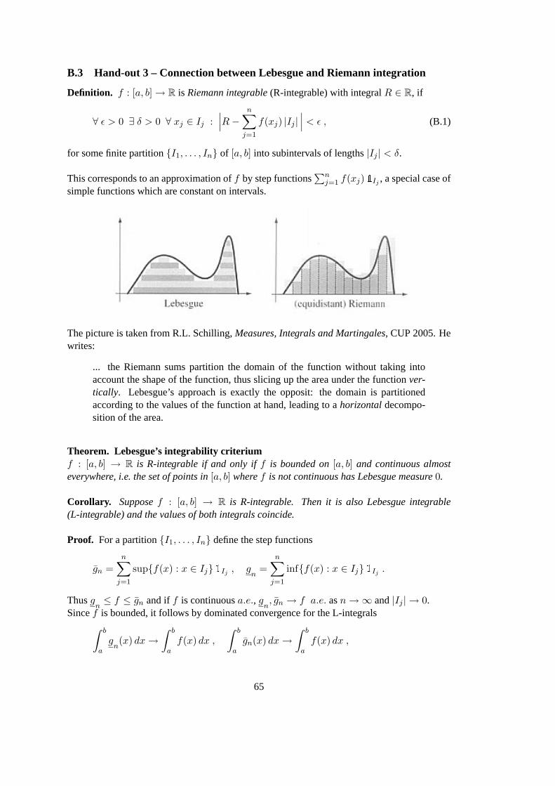
B.3 Hand-out 3 – Connection between Lebesgue and Riemann integration

Definition. f : [a, b] → R is Riemann integrable(R-integrable) with integralR ∈ R, if

∀ ε > 0 ∃ δ > 0 ∀ xj ∈ Ij :∣∣∣R−

n∑j=1

f(xj) |Ij |∣∣∣ < ε , (B.1)

for some finite partitionI1, . . . , In of [a, b] into subintervals of lengths|Ij | < δ.

This corresponds to an approximation off by step functions∑n

j=1 f(xj)1Ij , a special case ofsimple functions which are constant on intervals.

The picture is taken from R.L. Schilling,Measures, Integrals and Martingales, CUP 2005. Hewrites:

... the Riemann sums partition the domain of the function without taking intoaccount the shape of the function, thus slicing up the area under the functionver-tically. Lebesgue’s approach is exactly the opposit: the domain is partitionedaccording to the values of the function at hand, leading to ahorizontaldecompo-sition of the area.

Theorem. Lebesgue’s integrability criteriumf : [a, b] → R is R-integrable if and only iff is bounded on[a, b] and continuous almosteverywhere, i.e. the set of points in[a, b] wheref is not continuous has Lebesgue measure0.

Corollary. Supposef : [a, b] → R is R-integrable. Then it is also Lebesgue integrable(L-integrable) and the values of both integrals coincide.

Proof. For a partitionI1, . . . , In define the step functions

gn =n∑

j=1

supf(x) : x ∈ Ij1Ij , gn

=n∑

j=1

inff(x) : x ∈ Ij1Ij .

Thusgn≤ f ≤ gn and iff is continuousa.e., g

n, gn → f a.e. asn →∞ and|Ij | → 0.

Sincef is bounded, it follows by dominated convergence for the L-integrals∫ b

ag

n(x) dx →

∫ b

af(x) dx ,

∫ b

agn(x) dx →

∫ b

af(x) dx ,

65

so the sum in (B.1) converges and R =∫ ba f(x) dx .

On the other hand, if the sum in (B.1) converges, then∫ ba

∣∣gn(x)− gn(x)

∣∣ dx → 0 and thusfor the limit functionsg = g a.e., andf is continuousa.e. sinceg ≤ f ≤ g .If f was not bounded, one could choosexj in (B.1) such that the sum does not converge.2

On the other hand, not every L-integrable function is also R-integrable. The standard exampleis f = 1[0,1]∩Q , which can be made R-integrable by changing it on a set of L-measure0.This might suggest that for every L-integrablef there exists an R-integrableg with f = g a.e. .

This is not true as demonstrated by the following example:Let r1, r2 . . . be an enumeration of the rationals in(0, 1). For smallε > 0 and eachn ∈ Nchoose an open intervalIn ⊆ (0, 1) with rn ∈ In and L-measureµ(In) < ε 2−n. PutA =

⋃n In. ThenA is dense in(0, 1) with 0 < µ(A) < ε and thus for any non-degenerate

subintervalI of (0, 1), µ(A ∩ I) > 0.Takef = 1A and suppose thatf = g a.e.. LetIj be some decomposition of(0, 1) intosubintervals. Since for eachj, µ

(Ij ∩A∩ f = g

)= µ(Ij ∩A) > 0, g(xj) = f(xj) = 1 for

somexj ∈ Ij ∩A, and thus

n∑j=1

g(xj) µ(Ij) = 1 > µ(A) . (B.2)

If g were R-integrable, its integral would have to coincide with the L-integral∫ 10 f dµ = µ(A),

which is in contradiction to (B.2).

B.4 Hand-out 4 – Ergodic theorems

Hand-out 4 contains statements and proofs of Lemma 6.5 and Theorems 6.6 and 6.7, whichcan be found in Section 6.3.

66