probabilistic risk and safety
DESCRIPTION
this book gives fundamental knowledge of psaTRANSCRIPT


robabilistic Risk Assessmentand Managementfor Engineers and Scientists

IEEE Press445 Hoes Lane, ~O. Box ]331
Piscataway, NJ 08855-1331
Editorial BoardJ. B. Anderson, Editor in Chief
R. S. BlicqS. BlanchardM. EdenR. HerrickG. F. Hoffnagle
R. F. HoytS. V. KartalopoulosP. LaplanteJ. M. F. Moura
R. S. MullerI. PedenW. D. ReeveE. Sanchez-SinencioD. J. Wells
Dudley R. Kay, Director ofBook PublishingCarrie Briggs, Administrative Assistant
Lisa S. Mizrahi, Review and Publicity Coordinator
Valerie Zaborski, Production Editor
IEEE Reliability Society, Sponsor
RS-S Liaison to IEEE PressDev G. Raheja
Technical Reviewer
Yovan Lukic
Arizona Public Service Company
robabilistic RiskAssessment and Managementfor Engineers and Scientists
Hiromitsu KumamotoKyoto University
Ernest J. HenleyUniversity of Houston
IEEEPRESS
IEEE Reliability Society, Sponsor
The Institute of Electrical and Electronics Engineers, Inc., New York

This bookmaybepurchased at a discount from thepublisher when orderedinbulkquantities. Formore information contact:
IEEE PRESS MarketingAttn: Special Sales~O. Box 1331445 Hoes LanePiscataway, NJ 08855-1331Fax: +1 (732) 981-9334
©1996by the Institute of Electrical and Electronics Engineers, Inc.3 Park Avenue, 17th Floor, NewYork, NY 10016-5997
All rights reserved. No part of this book may be reproduced in any form,nor may it be stored in a retrieval system or transmitted in any form,without written permission from the publisher:
10 9 8 7 6 5 4 3 2
ISBN 0-7803-6017-6
IEEE Order Number: PP3533
The Library of Congress has catalogued the hard cover edition of this title as follows:
Kumamoto, Hiromitsu.Probabilistic risk assessment and management for engineers and
scientists I Hiromitsu Kumamoto, Ernest 1. Henley. -2nd ed.p. cm.
Rev. ed. of: Probabilistic risk assessment I Ernest 1. Henley.Includes bibliographical references and index.ISBN 0-7803-1004-7I. Reliability (Engineering) 2. Health risk assessment.
I. Henley, Ernest 1. II. Henley, Ernest 1. Probabilistic riskassessment. III. Title.
TS173.K86 1996 95-36502620'.00452-dc20 eIP
ontents
PREFACE xv
1 BASIC RISK CONCEPTS 1
1.1 Introduction 11.2 Formal Definition of Risk 1
1.2.1 Outcomes and Likelihoods 11.2.2 Uncertainty and Meta-Uncertainty 41.2.3 Risk Assessment and Management 61.2.4 Alternatives and Controllability of Risk 81.2.5 Outcome Significance 121.2.6 Causal Scenario 141.2.7 Population Affected 151.2.8 Population Versus Individual Risk 151.2.9 Summary 18
1.3 Source of Debates 181.3.1 Different Viewpoints Toward Risk 181.3.2 Differences in Risk Assessment 191.3.3 Differences in Risk Management 221.3.4 Summary 26
1.4 Risk-Aversion Mechanisms 261.4.1 Risk Aversion 271.4.2 Three Attitudes Toward Monetary Outcome 271.4.3 Significance of Fatality Outcome 301.4.4 Mechanisms for Risk Aversion 311.4.5 Bayesian Explanation of Severity Overestimation 311.4.6 Bayesian Explanation of Likelihood Overestimation 32
v
vi
1.4.7 PRAM Credibility Problem 351.4.8 Summary 35
1.5 Safety Goals 351.5.1 Availability, Reliability, Risk, and Safety 351.5.2 Hierarchical Goals for PRAM 361.5.3 Upper and Lower Bound Goals 371.5.4 Goals for Normal Activities 421.5.5 Goals for Catastrophic Accidents 431.5.6 Idealistic Versus Pragmatic Goals 481.5.7 Summary 52
References 53Problems 54
2 ACCIDENT MECHANISMS AND RISKMANAGEMENT 55
2.1 Introduction 552.2 Accident-Causing Mechanisms 55
2.2.1 Common Features of Plants with Risks 552.2.2 Negative Interactions Between Humans and the Plant 572.2.3 A Taxonomy of Negative Interactions 582.2.4 Chronological Distribution of Failures 622.2.5 Safety System and Its Malfunctions 642.2.6 Event Layer and Likelihood Layer 672.2.7 Dependent Failures and Management Deficiencies 722.2.8 Summary 75
2.3 Risk Management 752.3.1 Risk-Management Principles 752.3.2 Accident Prevention and Consequence Mitigation 782.3.3 Failure Prevention 782.3.4 Propagation Prevention 812.3.5 Consequence Mitigation 842.3.6 Summary 85
2.4 Preproduction Quality Assurance Program 852.4.1 Motivation 862.4.2 Preproduction Design Process 862.4.3 Design Review for PQA 872.4.4 Management and Organizational Matters 922.4.5 Summary 93
References 93Problems 94
3 PROBABILISTIC RISK ASSESSMENT 95
3.1 Introduction to Probabilistic Risk Assessment 953.1.1 Initiating-Event and Risk Profiles 953.1.2 Plants without Hazardous Materials 96
Contents

Contents
3.1.3 Plants with Hazardous Materials 973.1.4 Nuclear Power Plant PRA: WASH-1400 983.1.5 WASH-1400 Update: NUREG-1150 1023.1.6 Summary 104
3.2 Initiating-Event Search 1043.2.1 Searching for Initiating Events 1043.2.2 Checklists 1053.2.3 Preliminary Hazard Analysis 1063.2.4 Failure Mode and Effects Analysis 1083.2.5 FMECA 1103.2.6 Hazard and Operability Study 1133.2.7 Master Logic Diagram 1153.2.8 Summary 115
3.3 The Three PRA Levels 1173.3.1 Levell PRA-Accident Frequency 1173.3.2 Level 2 PRA-Accident Progression and Source Term 1263.3.3 Level 3 PRA-Offside Consequence 1273.3.4 Summary 127
3.4 Risk Calculations 1283.4.1 The Level 3 PRA Risk Profile 1283.4.2 The Level 2 PRA Risk Profile 1303.4.3 The Levell PRA Risk Profile 1303.4.4 Uncertainty of Risk Profiles 1313.4.5 Summary 131
3.5 Example of a Level 3 PRA 1323.6 Benefits, Detriments, and Successes of PRA 132
3.6.1 Tangible Benefits in Design and Operation 1323.6.2 Intangible Benefits 1333.6.3 PRA Negatives 1343.6.4 Success Factors of PRA Program 1343.6.5 Summary 136
References 136Chapter Three Appendices 138
A.l Conditional and Unconditional Probabilities 138A.1.1 Definition of Conditional Probabilities 138A.1.2 Chain Rule 139A.1.3 Alternative Expression of Conditional Probabilities 140A.1.4 Independence 140A.1.5 Bridge Rule 141A.1.6 Bayes Theorem for Discrete Variables 142A.1.7 Bayes Theorem for Continuous Variables 143
A.2 Venn Diagrams and Boolean Operations 143A.2.1 Introduction 143A.2.2 Event Manipulations via Venn Diagrams 144A.2.3 Probability and Venn Diagrams 145A.2.4 Boolean Variables and Venn Diagrams 146A.2.5 Rules for Boolean Manipulations 147
vii

viii Contents
A.3 A Level for 3 PRA-Station Blackout 148A.3.1 Plant Description 148A.3.2 Event Tree for Station Blackout 150A.3.3 Accident Sequences 152A.3.4 Fault Trees 152A.3.5 Accident-Sequence Cut Sets 153A.3.6 Accident-Sequence Quantification 155A.3.7 Accident-Sequence Group 156A.3.8 Uncertainty Analysis 156A.3.9 Accident-Progression Analysis 156A.3.10 Summary 163
Problems 163
4 FAULT-TREE CONSTRUCTION 165
4.1 Introduction 1654.2 Fault Trees 1664.3 Fault-Tree Building Blocks 166
4.3.1 Gate Symbols 1664.3.2 Event Symbols 1724.3.3 Summary 174
4.4 Finding Top Events 1754.4.1 Forward and Backward Approaches 1754.4.2 Component Interrelations and System Topography 1754.4.3 Plant Boundary Conditions 1764.4.4 Example of Preliminary Forward Analysis 1764.4.5 Summary 179
4.5 Procedure for Fault-Tree Construction 1794.5.1 Fault-Tree Example 1804.5.2 Heuristic Guidelines 1844.5.3 Conditions Induces by OR and AND Gates 1884.5.4 Summary 194
4.6 Automated Fault-Tree Synthesis 1964.6.1 Introduction 1964.6.2 System Representation by Semantic Networks 1974.6.3 Event Development Rules 2044.6.4 Recursive Three-Value Procedure for FT Generation 2064.6.5 Examples 2104.6.6 Summary 220
References 222Problems 223
5 QUALITATIVE ASPECTS OF SYSTEM ANALYSIS 227
5.1 Introduction 2275.2 Cut Sets and Path Sets 227
5.2.1 Cut Sets 2275.2.2 Path Sets (Tie Sets) 227
Contents
5.2.3 Minimal Cut Sets 2295.2.4 Minimal Path Sets 2295.2.5 Minimal Cut Generation (Top-Down) 2295.2.6 Minimal Cut Generation (Bottom-Up) 2315.2.7 Minimal Path Generation (Top-Down) 2325.2.8 Minimal Path Generation (Bottom-Up) 2335.2.9 Coping with Large Fault Trees 234
5.3 Common-Cause Failure Analysis 2405.3.1 Common-Cause Cut Sets 2405.3.2 Common Causes and Basic Events 2415.3.3 Obtaining Common-Cause Cut Sets 242
5.4 Fault-Tree Linking Along an Accident Sequence 2465.4.1 Simple Example 2465.4.2 A More Realistic Example 248
5.5 Noncoherent Fault Trees 2515.5.1 Introduction 2515.5.2 Minimal Cut Sets for a Binary Fault Tree 2525.5.3 Minimal Cut Sets for a Multistate Fault Tree 257
References 258Problems 259
6 QUANTIFICATIONOF BASIC EVENTS 263
6.1 Introduction 2636.2 Probabilistic Parameters 264
6.2.1 A Repair-to-Failure Process 2656.2.2 A Repair-Failure-Repair Process 2716.2.3 Parameters of Repair-to-Failure Process 2746.2.4 Parameters of Failure-to-Repair Process 2786.2.5 Probabilistic Combined-Process Parameters 280
6.3 Fundamental RelationsAmong Probabilistic Parameters 2856.3.1 Repair-to-Failure Parameters 2856.3.2 Failure-to-Repair Parameters 2896.3.3 Combined-Process Parameters 290
6.4 Constant-Failure Rate and Repair-Rate Model 2976.4.1 Repair-to-Failure Process 2976.4.2 Failure-to-Repair Process 2996.4.3 Laplace Transform Analysis 2996.4.4 Markov Analysis 303
6.5 Statistical Distributions 3046.6 General Failure and Repair Rates 3046.7 Estimating Distribution Parameters 309
6.7.1 Parameter Estimationfor Repair-to-Failure Process 309
6.7.2 Parameter Estimationfor Failure-to-Repair Process 318
ix

x
6.8 Components with Multiple Failure Modes 3226.9 Environmental Inputs 325
6.9.1 Command Failures 3256.9.2 Secondary Failures 325
6.10 Human Error 3266.11 System-Dependent Basic Event 326
References 327Chapter Six Appendices 327
A.l Distributions 327A.l.l Mean 328A.l.2 Median 328A.l.3 Mode 328A.l.4 Variance and Standard Deviation 328A.l.5 Exponential Distribution 329A.l.6 Normal Distribution 330A.l.7 Log-Normal Distribution 330A.l.8 Weibull Distribution 330A.l.9 Binomial Distribution 331A.l.lO Poisson Distribution 331A.l.ll Gamma Distribution 332A.l.12 Other Distributions 332
A.2 A Constant-Failure-Rate Property 332A.3 Derivation of Unavailability Formula 333A.4 Computational Procedure for Incomplete Test Data 334A.5 Median-Rank Plotting Position 334A.6 Failure and Repair Basic Definitions 335
Problems 335
7 CONFIDENCE INTERVALS 339
7.1 Classical Confidence Limits 3397.1.1 Introduction 3397.1.2 General Principles 3407.1.3 Types of Life-Tests 3467.1.4 Confidence Limits for Mean Time to Failure 3467.1.5 Confidence Limits for Binomial Distributions 349
7.2 Bayesian Reliability and Confidence Limits 3517.2.1 Discrete Bayes Theorem 3517.2.2 Continuous Bayes Theorem 3527.2.3 Confidence Limits 353
References 354Chapter Seven Appendix 354
A.l The x2, Student's t, and F Distributions 354A.l.l X2 Distribution Application Modes 355A.l.2 Student's t Distribution Application Modes 356
Contents

Contents
A.1.3 F Distribution Application Modes 357
Problems 359
xi
8 QUANTITATIVE ASPECTS OF SYSTEM ANALYSIS 363
8.1 Introduction 3638.2 Simple Systems 365
8.2.1 Independent Basic Events 3658.2.2 AND Gate 3668.2.3 OR Gate 3668.2.4 Voting Gate 3678.2.5 Reliability Block Diagrams 371
8.3 Truth-Table Approach 3748.3.1 AND Gate 3748.3.2 OR Gate 374
8.4 Structure-Function Approach 3798.4.1 Structure Functions 3798.4.2 System Representation 3798.4.3 Unavailability Calculations 380
8.5 Approaches Based on Minimal Cutsor Minimal Paths 3838.5.1 Minimal Cut Representations 3838.5.2 Minimal Path Representations 3848.5.3 Partial Pivotal Decomposition 3868.5.4 Inclusion-Exclusion Formula 387
8.6 Lower and Upper Boundsfor System Unavailability 3898.6.1 Inclusion-Exclusion Bounds 3898.6.2 Esary and Proschan Bounds 3908.6.3 Partial Minimal Cut Sets and Path Sets 390
8.7 System Quantification by KITT 3918.7.1 Overview ofKITT 3928.7.2 Minimal Cut Set Parameters 3978.7.3 System Unavailability Qs(t) 4028.7.4 System Parameter ws(t) 4048.7.5 Other System Parameters 4098.7.6 Short-Cut Calculation Methods 4108.7.7 The Inhibit Gate 4148.7.8 Remarks on Quantification Methods 415
8.8 Alarm Function and Two Types of Failure 4168.8.1 Definition of Alarm Function 4168.8.2 Failed-Safe and Failed-Dangerous Failures 4168.8.3 Probabilistic Parameters 419
References 420Problems 421

xii
9 SYSTEM QUANTIFICATIONFOR DEPENDENT EVENTS 425
9.1 Dependent Failures 4259.1.1 Functional and Common-Unit Dependency 4259.1.2 Common-Cause Failure 4269.1.3 Subtle Dependency 4269.1.4 System-Quantification Process 426
9.2 Markov Model for Standby Redundancy 4279.2.1 Hot, Cold, and Warm Standby 4279.2.2 Inclusion-Exclusion Formula 4279.2.3 Time-Dependent Unavailability 4289.2.4 Steady-State Unavailability 4399.2.5 Failures per Unit Time 4429.2.6 Reliability and Repairability 444
9.3 Common-Cause Failure Analysis 4469.3.1 Subcomponent-Level Analysis 4469.3.2 Beta-Factor Model 4499.3.3 Basic-Parameter Model 4569.3.4 Multiple Greek Letter Model 4619.3.5 Binomial Failure-Rate Model 4649.3.6 Markov Model 467
References 469Problems 469
10 HUMAN RELIABILITY 471
10.1 Introduction 47110.2 Classifying Human Errors for PRA 472
10.2.1 Before an Initiating Event 47210.2.2 During an Accident 472
10.3 Human and Computer Hardware System 47410.3.1 The Human Computer 47410.3.2 Brain Bottlenecks 47710.3.3 Human Performance Variations 478
10.4 Performance-Shaping Factors 48110.4.1 Internal PSFs 48110.4.2 External PSFs 48410.4.3 Types of Mental Processes 487
10.5 Human-Performance Quantification by PSFs 48910.5.1 Human-Error Rates and Stress Levels 48910.5.2 Error Types, Screening Values 49110.5.3 Response Time 49210.5.4 Integration of PSFs by Experts 49210.5.5 Recovery Actions 494
10.6 Examples of Human Error 49410.6.1 Errors in Thought Processes 49410.6.2 Lapse/Slip Errors 497
Contents

Contents
10.7 SHARP: General Framework 49810.8 THERP: Routine and Procedure-Following Errors 499
10.8.1 Introduction 49910.8.2 General THERP Procedure 502
10.9 HCR: Nonresponse Probability 50610.10 Wrong Actions due to Misdiagnosis 509
10.10.1 Initiating-Event Confusion 50910.10.2 Procedure Confusion 51010.10.3 Wrong Actions due to Confusion 510
References 511Chapter Ten Appendices 513
A.1 THERP for Errors During a Plant Upset 513A.2 HCR for Two Optional Procedures 525A.3 Human-Error Probability Tables from Handbook 530
Problems 533
xiii
11 UNCERTAINTY QUANTIFICATION 535
11.1 Introduction 53511.1.1 Risk-Curve Uncertainty 53511.1.2 Parametric Uncertainty and Modeling Uncertainty 53611.1.3 Propagation of Parametric Uncertainty 536
11.2 Parametric Uncertainty 53611.2.1 Statistical Uncertainty 53611.2.2 Data Evaluation Uncertainty 53711.2.3 Expert-Evaluated Uncertainty 538
11.3 Plant-Specific Data 53911.3.1 Incorporating Expert Evaluation as a Prior 53911.3.2 Incorporating Generic Plant Data as a Prior 539
11.4 Log-Normal Distribution 54111.4.1 Introduction 54111.4.2 Distribution Characteristics 54111.4.3 Log-Normal Determination 54211.4.4 Human-Error-Rate Confidence Intervals 54311.4.5 Product of Log-Normal Variables 54511.4.6 Bias and Dependence 547
11.5 Uncertainty Propagation 54911.6 Monte Carlo Propagation 550
11.6.1 Unavailability 55011.6.2 Distribution Parameters 55211.6.3 Latin Hypercube Sampling 553
11.7 Analytical Moment Propagation 55511.7.1 AND Gate 55511.7.2 OR Gate 55611.7.3 AND and OR Gates 55711.7.4 Minimal Cut Sets 558
xiv
11.7.5 Taylor Series Expansion 56011.7.6 Orthogonal Expansion 561
11.8 Discrete Probability Algebra 56411.9 Summary 566
References 566Chapter Eleven Appendices 567
A.1 Maximum-Likelihood Estimator 567A.2 Cut Set Covariance Formula 569A.3 Mean and Variance by Orthogonal Expansion 569
Problems 571
12 LEGAL AND REGULATORY RISKS 573
12.1 Introduction 57312.2 Losses Arising from Legal Actions 574
12.2.1 Nonproduct Liability Civil Lawsuits 57512.2.2 Product Liability Lawsuits 57512.2.3 Lawsuits by Government Agencies 57612.2.4 Worker's Compensation 57712.2.5 Lawsuit-Risk Mitigation 57812.2.6 Regulatory Agency Fines: Risk Reduction Strategies 579
12.3 The Effect of Government Regulationson Safety and Quality 58012.3.1 Stifling of Initiative and Abrogation of Responsibility 58112.3.2 Overregulation 582
12.4 Labor and the Safe Workplace 58312.4.1 Shaping the Company's Safety Culture 58412.4.2 The Hiring Process 584
12.5 Epilogue 587
INDEX 589
Contents
reface
Our previous IEEE Press book, Probabilistic Risk Assessment, was directed primarily atdevelopment of the mathematical tools required for reliability and safety studies. The titlewas somewhat a misnomer; the book contained very little material pertinent to the qualitativeand management aspects of the factors that place industrial enterprises at risk.
This book has a different focus. The (updated) mathematical techniques materialin our first book has been contracted by elimination of specialized topics such as vari-ance reduction Monte Carlo techniques, reliability importance measures, and storage tankproblems; the expansion has been entirely in the realm of management trade-offs of riskversus benefits. Decisions involving trade-offs are complex, and not easily made. Primi-tive academic models serve little useful purpose, so we decided to pursue the path of mostresistance, that is, the inclusion of realistic, complex examples. This, plus the fact that webelieve engineers should approach their work with a mathematical-not a trade school-mentality, makes this book difficult to use as an undergraduate text, even though all requiredmathematical tools are developed as appendices. We believe this book is suitable as an un-dergraduate plus a graduate text, so a syllabus and end-of-chapter problems are included.The book is structured as follows:
Chapter 1: Formal definitions of risk, individual and population risk, risk aversion,safety goals, and goal assessments are provided in terms of outcomes and likelihoods.Idealistic and pragmatic goals are examined.
Chapter 2: Accident-causing mechanisms are surveyed and classified. Coupling,dependency, and propagation mechanisms are discussed. Risk-management princi-ples are described. Applications to preproduction quality assurance programs arepresented.
Chapter 3: Probabilistic risk assessment (PRA) techniques, including event trees, pre-liminary hazard analyses, checklists, failure mode and effects analysis, hazard and
xv
xvi Preface
operability studies, and fault trees, are presented, and staff requirements and manage-ment considerations are discussed. The appendix includes mathematical techniquesand a detailed PRA example.
Chapter 4: Fault-tree symbols and methodology are explored. A new, automated,fault-tree synthesis method based on flows, flow controllers, semantic networks, andevent development rules is described and demonstrated.
Chapter 5: Qualitative aspects of system analysis, including cut sets and path sets andthe methods of generating them, are described. Common-cause failures, multistatevariables, and coherency are treated.
Chapter 6: Probabilistic failure parameters such as failure and repair rates are definedrigorously and the relationships between component parameters are shown. Laplaceand Markov analyses are presented. Statistical distributions and their properties areconsidered.
Chapter 7: Confidence limits of failure parameters, including classical and Bayesianapproaches, form the contents of this chapter.
Chapter 8: Methods for synthesizing quantitative system behavior in terms of theoccurrence probability of basic failure events are developed and system performanceis described in terms of system parameters such as reliability, availability, and meantime to failure. Structure functions, minimal path and cut representations, kinetic-treetheory, and short-cut methods are treated.
Chapter 9: Inclusion-exclusion bounding, standby redundancy Markov transitiondiagrams, beta-factor, multiple Greek letter, and binomial failure rate models, whichare useful tools for system quantification in the presence of dependent basic events,including common-cause failures, are given. Examples are provided.
Chapter 10: Human-error classification, THERP (techniques for human error-rateprediction) methodology for routine and procedure-following error, HeR (humancognitive reliability) models for nonresponse error under time pressure, and con-fusion models for misdiagnosis are described to quantitatively assess human-errorcontributions to system failures.
Chapter 11: Parametric uncertainty and modeling uncertainty are examined. TheBayes theorem and log-normal distribution are used for treating parametric uncer-tainties that, when propagated to system levels, are treated by techniques such asLatin hypercube Monte Carlo simulations, analytical moment methods, and discreteprobability algebra.
Chapter 12: Aberrant behavior by lawyers and government regulators are shownto pose greater risks to plant failures than accidents. The risks are described andloss-prevention techniques are suggested.
In using this book as a text, the schedule and sequence of material for a three-credit-hour course are suggested in Tables 1 and 2. A solutions manual for all end-of-chapterproblems is available from the authors. Enjoy.
Chapter 12 is based on the experience of one of us (EJH) as director of MaxximMedical Inc. The author is grateful to the members of the Regulatory Affairs, HumanResources, and Legal Departments of Maxxim Medical Inc. for their generous assistanceand source material.
Preface xvii
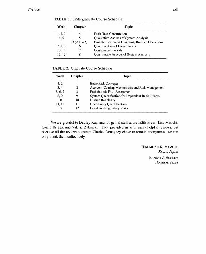
TABLE 1. Undergraduate Course Schedule
Week
1,2,34,5
67,8,910, 1112,13
Chapter
45
3(Al,A2)678
Topic
Fault-Tree ConstructionQualitative Aspects of System AnalysisProbabilities, Venn Diagrams, Boolean OperationsQuantification of Basic EventsConfidence IntervalsQuantitative Aspects of System Analysis
TABLE 2. Graduate Course Schedule
Week
1,23,4
5,6,78,910
11, 1213
Chapter
1239101112
Topic
Basic Risk ConceptsAccident-Causing Mechanisms and Risk ManagementProbabilistic Risk AssessmentSystem Quantification for Dependent Basic EventsHuman ReliabilityUncertainty QuantificationLegal and Regulatory Risks
We are grateful to Dudley Kay, and his genial staff at the IEEE Press: Lisa Mizrahi,Carrie Briggs, and Valerie Zaborski. They provided us with many helpful reviews, butbecause all the reviewers except Charles Donaghey chose to remain anonymous, we canonly thank them collectively.
HIROMITSU KUMAMOTO
Kyoto, Japan
ERNEST J. HENLEY
Houston, Texas

1asic Risk Concepts
1.1 INTRODUCTION
Risk assessment and risk management are two separate but closely related activities. Thefundamental aspects of these two activities are described in this chapter, which providesan introduction to subsequent developments. Section 1.2 presents a formal definition ofrisk with focus on the assessment and management phases. Sources of debate in currentrisk studies are described in Section 1.3. Most people perform a risk study to avoid seriousmishaps. This is called risk aversion, which is a kernel of risk management; Section 1.4describes risk aversion. Management requires goals; achievement of goals is checked byassessment. An overview of safety goals is given in Section 1.5.
1.2 FORMAL DEFINITION OF RISK
Risk is a word with various implications. Some people define risk differently from others.This disagreement causes serious confusion in the field of risk assessment and management.The Webster's Collegiate Dictionary, 5th edition, for instance, defines risk as the chanceof loss, the degree of probability of loss, the amount of possible loss, the type of lossthat an insurance policy covers, and so forth. Dictionary definitions such as these are notsufficiently precise for risk assessment and management. This section provides a formaldefinition of risk.
1.2.1 Outcomes and Likelihoods
Astronomers can calculate future movements of planets and tell exactly when thenext solar eclipse will occur. Psychics of the Delphi Temple of Apollo foretold the futureby divine inspiration. These are rare exceptions, however. Just as a TV weatherperson, most
1
2 Basic Risk Concepts • Chap. J
people can only forecast or predict the future with considerable uncertainty. Risk is aconcept attributable to future uncertainty.
Primary definition ofrisk. A weather forecast such as "30 percent chance of raintomorrow" gives two outcomes together with their likelihoods: (30%, rain) and (70%, norain). Risk is defined as a collection of such pairs of likelihoods and outcomes:*
{(30%, rain), (70%, no rain)}.
More generally, assume n potential outcomes in the doubtful future. Then risk isdefined as a collection of n pairs.
(1.1)
where 0; and L; denote outcome i and its likelihood, respectively. Throwing a dice yieldsthe risk,
Risk == {(1/6, 1), (1/6,2), ... , (1/6, 6)} (1.2)
where the outcome is a particular face and the likelihood is probability I in 6.In situations involving random chance, each face involves a beneficial or a harmful
event as an ultimate outcome. When the faces are replaced by these outcomes, the risk ofthrowing the die can be rewritten more explicitly as
(1.3)
Risk profile. The distribution pattern of the likelihood-outcome pair is called a riskprofile (or a risk curve); likelihoods and outcomes are displayed along vertical and horizontalaxes, respectively. Figure 1.1 shows a simple risk profile for the weather forecast describedearlier; two discrete outcomes are observed along with their likelihoods, 30% rain or 70%no rain.
In some cases, outcomes are measured by a continuous scale, or the outcomes are somany that they may be continuous rather than discrete. Consider an investment problemwhere each outcome is a monetary return (gain or loss) and each likelihood is a densityof experiencing a particular return. Potential pairs of likelihoods and outcomes then forma continuous profile. Figure 1.2 is a density profile j'(x) where a positive or a negativeamount of money indicates loss or gain, respectively.
Objective versus subjective likelihood. In a perfect risk profile, each likelihood isexpressed as an objective probability, percentage, or density per action or per unit time, orduring a specified time interval (see Table 1.1). Objective frequencies such as two occur-rences per year and ratios such as one occurrence in one million are also likelihoods; if thefrequency is sufficiently small, it can be regarded as a probability or a ratio. Unfortunately,the likelihood is not always exact; probability, percentage, frequency, and ratios may bebased on subjective evaluation. Verbal probabilities such as rare, possible, plausible, andfrequent are also used.
*Toavoid proliferationof technical terms,a hazard or a danger is definedin this bookas a particularprocessleading to an undesirable outcome. Risk is a whole distribution pattern of outcomes and likelihoods; differenthazards may constitute the risk "fatality," that is, various natural or man-made phenomena may cause fatalitiesthrough a varietyof processes. The hazardor danger is akin to a causal scenario, and is a moreelementaryconceptthan risk.

Sec. 1.2 • Formal Definition ofRisk 3
Figure 1.1. Simple risk profile from aweather forecast.
80 r-'
70 f-
60 f-
~ 50 f--~
'Ca
40 f-a£:Qj~ 30 f-::i
20 r-
10 r-
0
No Rain-
Outcome
Rain.---
.i?:''u;CQl
oQlUC~::J
8
-5 -4 -3 - 2 - 1Gain
1.0
0.9
0.8
0.7
0.6
0.5
0.4
0.3
0.2
0.1
o 2 x 3Loss
4 5
Monetary Outcome
~)(:c VIell'C.c Qla Ql.... Ua.. xVI QlVI VIQl VIu aX-lw~
-5 - 4 -3 - 2 -1Gain
o
p
2 x 3Loss
4 5
Monetary Outcome
Figure 1.2. Occurrence density and complementary cumulative risk profile.

4 Basic Risk Concepts • Chap. J
TABLE 1.1. Examples of Likelihood and Outcome
Measure
Likelihood
UnitOutcomeCategory
ProbabiIityPercentageDensityFrequencyRatioVerbal Expression
Per ActionPer Demand or OperationPer UnitTimeDuring LifetimeDuringTime IntervalPer Mileage
PhysicalPhysiologicalPsychologicalFinancialTime, OpportunitySocietal, Political
Complementary cumulative profile. The risk profile (discrete or continuous) isoften displayed in terms of complementary cumulative likelihoods. For instance, the like-lihood F(x) == fxoo
j'(u)du of losing x or more money is displayed rather than the densityj'(x) of just losing x. The second graph of Figure 1.2 shows a complementary cumulativerisk profile obtained from the density profile shown by the first graph. Point P on the ver-tical axis denotes the probability of losing zero or more money, that is, a probability of notgetting any profit. The complementary cumulative likelihood is a monotonously decreas-ing function of variable x, and hence has a simpler shape than the density function. Thecomplementary representation is informative because decision makers are more interestedin the likelihood of losing x or more money than in just x amount of money; for instance,they want to know the probability of "no monetary gain," denoted by point P in the secondgraph of Figure 1.2.
Farmer curves. Figure 1.3 shows a famous example from the Reactor Safety Study[1] where annual frequencies of x or more early fatalities caused by 100 nuclear powerplants are predicted and compared with fatal frequencies by air crashes, fires, dam failures,explosions, chlorine releases, and air crashes. Nonnuclear frequencies are normalizedby a size of population potentially affected by the 100 nuclear power plants; these arenot frequencies observed on a worldwide scale. Each profile in Figure 1.3 is called aFarmer curve [2]; horizontal and vertical axes generally denote the accident severity andcomplementary cumulative frequency per unit time, respectively.
Only fatalities greater than or equal to 10 are displayed in Figure 1.3. This is anexceptional case. Fatalities usually start with unity; in actual risk problems, a zero fatalityhas a far larger frequency than positive fatalities. Inclusion of a zero fatality in the Farmercurve requires the display of an unreasonably wide range of likelihoods.
1.2.2 Uncertainty and Meta-Uncertainty
Uncertainty. A kernel element of risk is uncertainty represented by plural out-comes and their future likelihoods. This point is emphasized by considering cases withoutuncertainty.
Outcome guaranteed. No risk exists if the future outcome is uniquely known (i.e.,n == I) and hence guaranteed. We will all die some day. The probability is equal to 1,so there would be no fatal risk if a sufficiently long time frame is assumed. The rain riskdoes not exist if there was 100% assurance of rain tomorrow, although there would be otherrisks such as floods and mudslides induced by the rain. In a formal sense, any risk exists ifand only if more than one outcome (n ~ 2) are involved with positive likelihoods during aspecified future time interval. In this context, a situation with two opposite outcomes with

Sec. 1.2 • Formal Definition ofRisk
>< 10-1
C>C=0Q)Q)oxW 10-2
en~(ij«iu..'0 10-3
~ocQ)::JCTQ)u: 10-4
(ij::JCC«
-------.-------,--
. . .------ ..-------,.------- .. ------
103 104
Number of Fatalities, x
Figure 1.3. Comparison of annual frequency of x or more fatalities.
5
equal likelihoods may be the most risky one. In less formal usage, however, a situationis called more risky when severities (or levels) of negative outcomes or their likelihoodsbecome larger; an extreme case would be the certain occurrence of a negative outcome.
Outcome localized. A 10-6 lifetime likelihood of a fatal accident to the U.S. pop-ulation of 236 million implies 236 additional deaths over an average lifetime (a 70-yearinterval). The 236 deaths may be viewed as an acceptable risk in comparison to the 2 millionannual deaths in the United States [3].
Risk = (10-6, fatality): acceptable (1.4)
On the other hand, suppose that 236 deaths by cancer of all workers in a factory arecaused, during a lifetime, by some chemical intermediary totally confined to the factoryand never released into the environment. This number of deaths completely localized in the

6 Basic Risk Concepts • Chap. J
factory is not a risk in the usual sense. Although the ratio of fatalities in the U.S. populationremains unchanged, that is, 10-6/lifetime, the entire U.S. population is no longer suitableas a group of people exposed to the risk; the population should be replaced by the group ofpeople in the factory.
Risk == (1, fatality): unacceptable (1.5)
Thus a source of uncertainty inherent to the risk lies in the anonymity of the victims.If the names of victims were known in advance, the cause of the outcome would be acrime. Even though the number of victims (about 11,000 by traffic accidents in Japan)can be predicted in advance, the victims' names must remain unknown for risk problemformulation purposes.
If only one person is the potential victim at risk, the likelihood must be smaller thanunity. Assume that a person living alone has a defective staircase in his house. Thenonly one person is exposed to a possible injury caused by the staircase. The populationaffected by this risk consists of only one individual; the name of the individual is knownand anonymity is lost. The injury occurs with a small likelihood and the risk concept stillholds.
Outcome realized. There is also no risk after the time point when an outcomeis realized. The airplane risk for an individual passenger disappears after the landing orcrash, although he or she, if alive, now faces other risks such as automobile accidents. Theuncertainty in the risk exists at the prediction stage and before its realization.
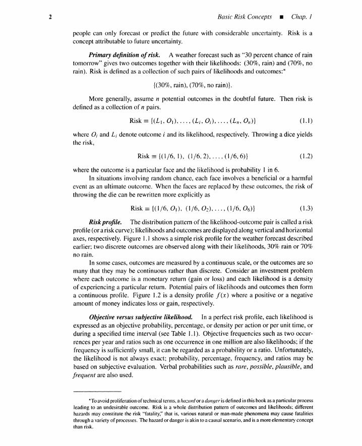
Meta-uncertainty. The risk profile itself often has associated uncertainties thatare called meta-uncertainties. A subjective estimate of uncertainties for a complementarycumulative likelihood was carried out by the authors of the Limerick Study [4]. Their resultis shown in Figure 1.4. The range of uncertainty stretches over three orders of magnitude.This is a fair reflection on the present state of the art of risk assessment. The error bandsare a result of two types of meta-uncertainties: uncertainty in outcome level of an accidentand uncertainty in frequency of the accident. The existence of this meta-uncertainty makesrisk management or decision making under risk difficult and controversial.
In summary, an ordinary situation with risk implies uncertainty due to plural out-comes with positive likelihoods, anonymity of victims, and prediction before realization.Moreover, the risk itself is associated with meta-uncertainty.
1.2.3 Risk Assessment and Management
Risk assessment. A principal purpose of risk assessment is the derivation of riskprofiles posed by a given situation; the weatherman performed a risk assessment when hepromulgated the risk profile in Figure 1.1. The Farmer curves in Figures 1.3 and 1.4 arefinal products of a methodology called probabilistic risk assessment (PRA), which, amongother things, enumerates outcomes and quantifies their likelihoods.
For nuclear power plants, the PRA proceeds as follows: enumeration of sequences ofevents that could produce a core melt; clarification ofcontainment failure modes, their prob-abilities and timing; identification of quantity and chemical form of radioactivity releasedif the containment is breached; modeling of dispersion of radionuclides in the atmosphere;modeling of emergency response effectiveness involving sheltering, evacuation, and med-ical treatment; and dose-response modeling in estimating health effects on the populationexposed [5].
Sec. 1.2 • Formal DefinitionofRisk 7
101 102 103 104
Number of Fatalities, x
10-10'------=----~--""----~--.;'----~----:.--~1
Figure 1.4. Example of meta-uncertainty of a complementary cumulative riskprofile.
Risk management. Risk management proposes alternatives, evaluates (for eachalternative) the risk profile, makes safety decisions, chooses satisfactory alternatives tocontrol the risk, and exercises corrective actions. *
Assessment versus management. When risk management is performed in relationto a PRA, the two activities are called a probabilistic risk assessment and management(PRAM). This book focuses on PRAM.
The probabilistic risk assessment phase is more scientific, technical, formal, quan-titative, and objective than the management phase, which involves value judgment andheuristics, and hence is more subjective, qualitative, societal, and political. Ideally, thePRA is based on objective likelihoods such as electric bulb failure rates inferred fromstatistical data and theories. However, the PRA is often compelled to use subjectivelikelihoods based on intuition, expertise, and partial, defective, or deceitful data, anddubious theories. These constitute the major source of meta-uncertainty in the riskprofile.
Considerable efforts are being made to establish a unified and scientific PRAMmethodology where subjective assessment, value judgment, expertise, and heuristics aredealt with more objectively. Nonetheless the subjective or human dimension does consti-tute one of the two pillars that support the entire conceptual edifice [3].
*Terms such as risk estimation and risk evaluation only cause confusion,and shouldbe avoided.
8 Basic Risk Concepts _ Chap. J
1.2.4 Alternatives and Controllability ofRisk
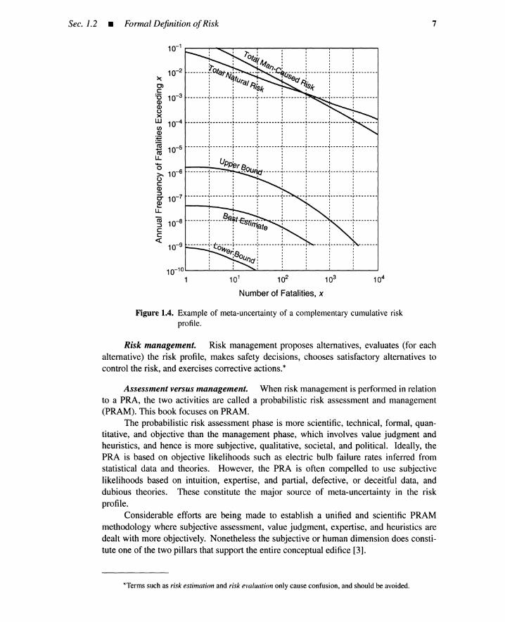
Example I-Daily risks. An interesting perspectiveon the risks of our daily activity wasdeveloped by Imperial Chemical Industries Ltd. [6]. The ordinate of Figure 1.5 is the fatal accidentfrequencyrate (FAFR),the averagenumberof deaths by accidents in 108 hoursof a particularactivity.An FAFRof unity corresponds to one fatality in 11,415years, or 87.6 fatalities per one million years.Thus a motor driver according to Figure 1.5 would, on the average, encounter a fatal accident if shedrove continuously 17years and 4 months, while a chemical industry workerrequires more than 3000years for his fatality. •
Key81 r,- a: eepmq irnel-
I- b: Eating, washing, dressing, etc., at home 660 660I- ...I- c: Driving to or from work by carI--
I- d: The day's work
l-e: The lunch breakf: Motorcycling
I- g: Commercial entertainment
-Construction Industry--- 57 57- ..- ......
---
-
--l-
I-
I-
r-- Chemical IndustryI- 3.5 3.5
3.0I- 2.5 2.5 2.5 2.5
r-- ~ I---- t0o-
l-
1.0~
I-- a b c d e d c b f 9 f b a
I I I I I I I I I I I I I I I I I I
0.5
100
Q) 50coa:>-oc:Q)::JsrQ)...u.E 10Q)
"C·0o 5«(ij15u.
500
2 4 6 8 10 12 14
Time (hour)
16 18 20 22 24
Figure 1.5. Fatal accident frequency rates of daily activities.
Risk control. The potential for plural outcomes and single realization by chancerecur endlessly throughout our lives. This recursion is a source of diversity in human affairs.Our lives would be monotonous if future outcomes were unique at birth and there were norisks at all; this book wouldbe useless too. Fortunately,enough or even an excessiveamountof risk surrounds us. Many people try to assess and manage risks; some succeed and oth-ers fail.
Sec. 1.2 • Formal DefinitionofRisk 9
Active versuspassive controllability. Although the weatherperson performs a riskassessment, he cannot alter the likelihood, because rain is an uncontrollable natural phe-nomenon. However, he can perform a risk management together with the assessment; hecan passively control or mitigate the rain hazard by suggesting that people take an umbrella;the outcome "rain" can be mitigated to "rain with umbrella."
Figure 1.5 shows seven sources (a to g) of the fatality risk. PRA deals with risksof human activities and systems found in engineering, economics, medicine, and so forth,where likelihoods of some outcomes can be controlled by active intervention, in additionto the passive mitigation of other outcomes.
Alternatives and controllability. Active or passive controllability of risks inherentlyassumes that each alternative chosen by a decision maker during the risk-management phasehas a specific risk profile. A baseline decision or action is also an alternative. In some cases,only the baseline alternative is available, and no room is left for choice. For instance, ifan umbrella is not available, people would go out without it. Similarly, passengers in acommercial airplane flying at 33,000 feet have only the one alternative of continuing theflight. In these cases, the risk is uncontrollable. Some alternatives have no appreciableeffect on the risk profile, while others bring desired effects; some are more cost effectivethan others.
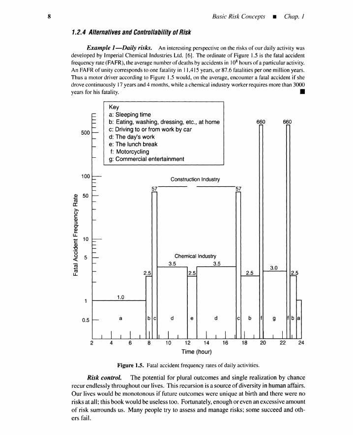
Example 2-Alternatives for rain hazard mitigation. Figure 1.6 shows a simple treefor the rain hazard mitigation problem. Two alternatives exist: 1) going out with an umbrella (A 1),
and 2) going out without an umbrella (A2). Four outcomes are observed: 1) 011 = rain, with um-brella; 2) 0 21 = no rain, with umbrella; 3) 0 12 = rain, without umbrella; and 4) 0 22 = no rain,without umbrella. The second subscript denotes a particular alternative, and the first a specific out-come under the alternative. In this simple example, the rain hazard is mitigated by the umbrella,though the likelihood (30%) of rain remains unchanged. Two different risk profiles appear, depend-ing on the alternative chosen, where R1 and R2 denote the risks with and without the umbrella,respectively:
R1 = {(30%, all), (70%, 02d}
R2 = {(30%, 012), (700/0, 0 22) }
------011: Rain, with Umbrella
"'------°21: No Rain, with Umbrella
r-------012: Rain, without Umbrella
...-.------ 022: No Rain,without Umbrella
Figure 1.6. Simple branching tree for rain hazard mitigation problem.
(1.6)
(1.7)
•

10 Basic Risk Concepts _ Chap. J
In general, a choice of particular alternative Aj yields risk profile Rj where likelihoodl-u- outcome Oi], and total number nj of outcomes vary from alternative to alternative:
j == 1, ... , m (1.8)
The subscript j denotes a particular alternative. This representation denotes an explicitdependence of the risk profile on the alternative.
Choices and alternatives exist in almost every activity: product design, manufacture,test, maintenance, personnel management, finance, commerce, health care, leisure, and soon. In the rain hazard mitigation problem in Figure 1.6, only outcomes could be mod-ified. In risk control problems for engineering systems, both likelihoods and outcomesmay be modified, for instance, by improving plant designs and operation and maintenanceprocedures. Operating the plant without modification or closing the operation are alsoalternatives.
Outcome matrix. A baseline risk profile changes to a new one when a differentalternative is chosen. For the rain hazard mitigation problem, two sets of outcomes exist, asshown in Table 1.2. The matrix showing the relation between the alternative and outcomeis called an outcome matrix. The column labeled utility will be described later.
TABLE 1.2. Outcome Matrix of Rain Hazard Mitigation Problem
Alternative Likelihood Outcome Utility
A 1: With umbrella L 11 = 30% 0 11: Rain, with umbrella U11 = I
L21 = 70% 0 21: No rain, with umbrella UZJ = 0.5
A2: Without umbrella L 12 = 30% 0 12: Rain, without umbrella U12 = 0
L 22 = 70% 0 22 : No rain, without umbrella U22 = 1
Lotteries. Assume that m alternatives are available. The choice of alternativeAj is nothing but a choice of lottery R, among the m lotteries, the term lottery beingused to indicate a general probabilistic set of outcomes. Two lotteries, R1 and R2, areavailable for the rain hazard mitigation problem in Figure 1.6; each lottery yields a particularstatistical outcome. There is a one-to-one correspondence among risk, risk profile, lottery,and alternative; these terms may be used interchangeably.
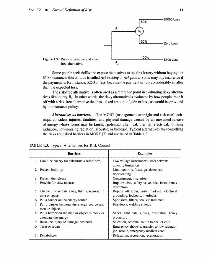
Risk-free alternatives. Figure 1.7 shows another situation with two exclusive al-ternatives A 1 and A2• When alternative A 1 is chosen, there is a fifty-fifty chance of losing$1000 or nothing; the expected loss is (1000 x 0.5) + (0 x 0.5) == $500. The secondalternative causes a certain loss of $500. In other words, only one outcome can occur whenalternative A2 is chosen; this is a risk-free alternative, as a payment for accident insuranceto compensate for the $1000 loss that occurs with probability 0.5. Alternative A 1 has twooutcomes and is riskier than alternative A2 because of the potential of the large $1000 loss.
It is generally believed that most people prefer a certain loss to the same amount ofexpected loss; that is, they will buy insurance for $500 to avoid lottery R I. This attitude iscalled risk aversion; they would not buy insurance, however, if the payment is more than$750, because the payment becomes considerably larger than the expected loss.
Sec. 1.2 • Formal Definition ofRisk 11
~----- $1000 Loss
'------- Zero Loss
100%"'------------- $500 LossFigure 1.7. Risky alternative and risk-
free alternative.
Some people seek thrills and expose themselves to the first lottery without buying the$500 insurance; this attitude is called risk seeking or risk prone. Some may buy insurance ifthe payment is, for instance, $250 or less, because the payment is now considerably smallerthan the expected loss.
The risk-free alternative is often used as a reference point in evaluating risky alterna-tives like lottery R I • In other words, the risky alternative is evaluated by how people trade itoff with a risk-free alternative that has a fixed amount of gain or loss, as would be providedby an insurance policy.
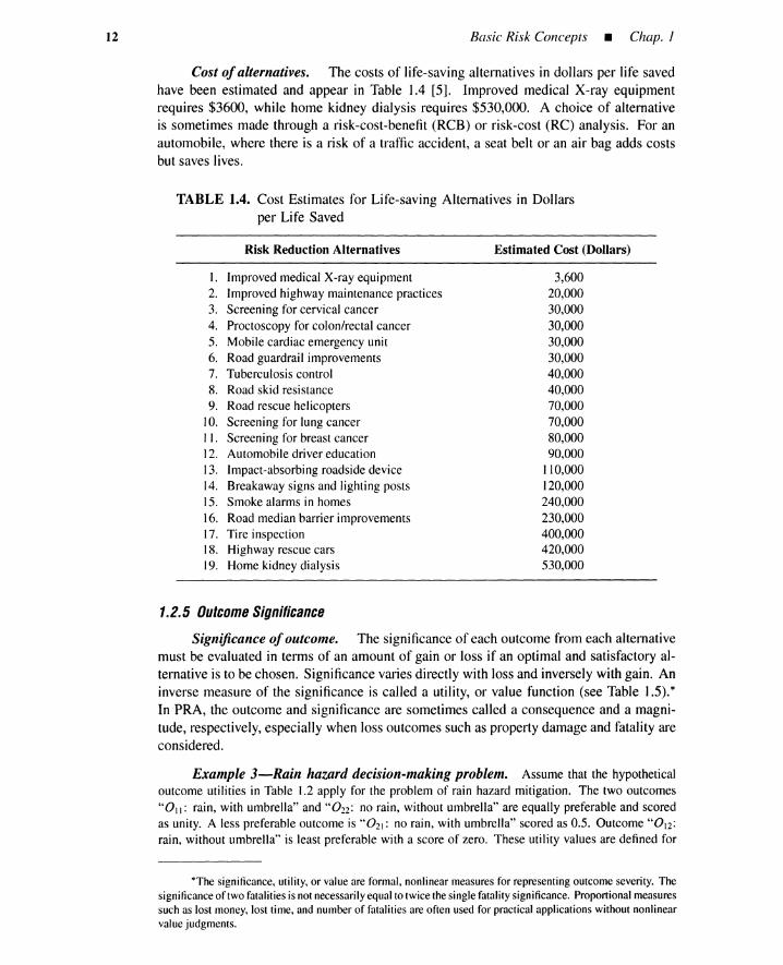
Alternatives as barriers. The MORT (management oversight and risk tree) tech-nique considers injuries, fatalities, and physical damage caused by an unwanted releaseof energy whose forms may be kinetic, potential, chemical, thermal, electrical, ionizingradiation, non-ionizing radiation, acoustic, or biologic. Typical alternatives for controllingthe risks are called barriers in MORT [7] and are listed in Table 1.3.
TABLE 1.3. Typical Alternatives for Risk Control
Barriers Examples
1. Limit the energy (or substitute a safer form)
2. Prevent build-up
3. Prevent the release4. Provide for slow release
5. Channel the release away, that is, separate intime or space
6. Put a barrier on the energy source7. Put a barrier between the energy source and
men or objects8. Put a barrier on the man or object to block or
attenuate the energy9. Raise the injury or damage threshold
10. Treat or repair
11. Rehabilitate
Low voltage instruments, safer solvents,quantity limitationLimit controls, fuses, gas detectors,floor loadingContainment, insulationRupture disc, safety valve, seat belts, shockabsorptionRoping off areas, aisle marking, electricalgrounding, lockouts, interlocksSprinklers, filters, acoustic treatmentFire doors, welding shields
Shoes, hard hats, gloves, respirators, heavyprotectorsSelection, acclimatization to heat or coldEmergency showers, transfer to low radiationjob, rescue, emergency medical careRelaxation, recreation, recuperation
12 Basic Risk Concepts • Chap. J
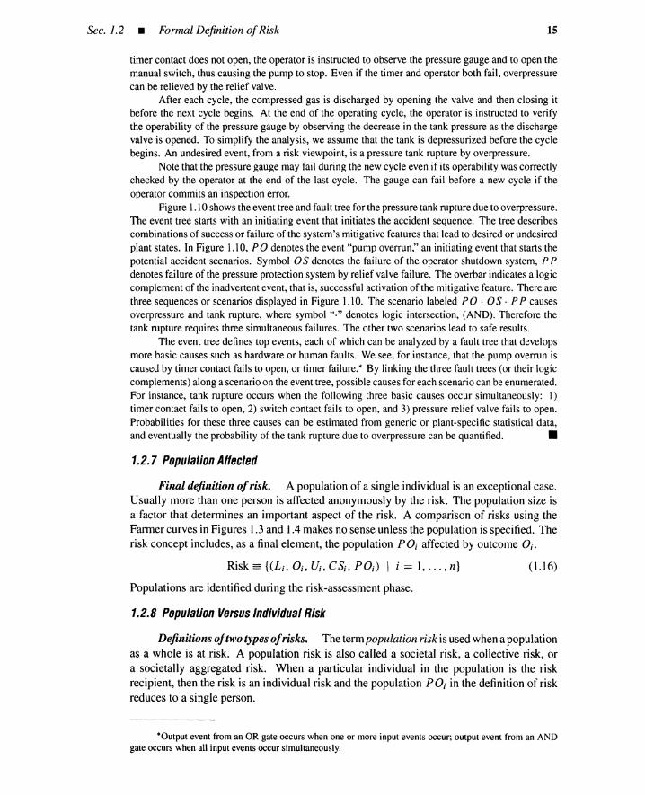
Cost ofalternatives. The costs of life-saving alternatives in dollars per life savedhave been estimated and appear in Table 1.4 [5]. Improved medical X-ray equipmentrequires $3600, while home kidney dialysis requires $530,000. A choice of alternativeis sometimes made through a risk-cost-benefit (RCB) or risk-cost (RC) analysis. For anautomobile, where there is a risk of a traffic accident, a seat belt or an air bag adds costsbut saves lives.
TABLE 1.4. Cost Estimates for Life-saving Alternatives in Dollarsper Life Saved
Risk Reduction Alternatives
I. Improved medical X-ray equipment2. Improved highway maintenance practices3. Screening for cervical cancer4. Proctoscopy for colon/rectal cancer5. Mobile cardiac emergency unit6. Road guardrail improvements7. Tuberculosis control8. Road skid resistance9. Road rescue helicopters
10. Screening for lung cancerI I. Screening for breast cancer12. Automobile driver education13. Impact-absorbing roadside device14. Breakaway signs and lighting posts15. Smoke alarms in homes16. Road median barrier improvements17. Tire inspection18. Highway rescue cars19. Home kidney dialysis
1.2.5 Outcome Significance
Estimated Cost (Dollars)
3,60020,00030,00030,00030,00030,00040,00040,00070,00070,00080,00090,000
110,000120,000240,000230,000400,000420,000530,000
Significance ofoutcome. The significance of each outcome from each alternativemust be evaluated in terms of an amount of gain or loss if an optimal and satisfactory al-ternative is to be chosen. Significance varies directly with loss and inversely with gain. Aninverse measure of the significance is called a utility, or value function (see Table 1.5).*In PRA, the outcome and significance are sometimes called a consequence and a magni-tude, respectively, especially when loss outcomes such as property damage and fatality areconsidered.
Example 3-Rain hazard decision-making problem. Assume that the hypotheticaloutcome utilities in Table 1.2 apply for the problem of rain hazard mitigation. The two outcomes"011: rain, with umbrella" and "022: no rain, without umbrella" are equally preferable and scoredas unity. A less preferable outcome is "021: no rain, with umbrella" scored as 0.5. Outcome "012:
rain, without umbrella" is least preferable with a score of zero. These utility values are defined for
*The significance,utility,or value are formal, nonlinear measures for representing outcome severity. Thesignificanceof two fatalitiesis not necessarilyequal to twice the single fatalitysignificance. Proportionalmeasuressuch as lost money, lost time, and number of fatalities are often used for practical applications without nonlinearvaluejudgments.

Sec. 1.2 • Formal Definition ofRisk
TABLE 1.5. Examples of Outcome Severity and Risk Level Measure
13
Outcome Severity Measure
SignificanceUtility, valueLost moneyFatalitiesLongevity lossDoseConcentrationLost time
Risk Level Measure
Expected significanceExpected utility or valueExpected money lossExpected fatalitiesExpected longevity lossExpected outcome severitySeverity for fixed outcomeLikelihood for fixed outcome
outcomes, not for the risk profile of each alternative. As shown in Figure 1.8, it is necessary tocreate a utility value (or a significance value) for each alternative or for each risk profile. Because theoutcomes occur statistically, an expected utility for the risk profile becomes a reasonable measure tounify the elementary utility values for outcomes in the profile.
P1°1,51
P2° 2,52
P3° 3,53
Figure 1.8. Risk profile significance de-rived from outcome signifi-cance.
5 i : Outcome Significance
Risk Profile Significance5= f(P 1, 51' P2 , 52' P3, 53)
The expected utility EUI for alternative A I is
EVI = (0.3 x VII) + (0.7 x VZI)
= (0.3 x 1) + (0.7 x 0.5) = 0.65
while the expected utility EUz for alternative Az is
EUz = (0.3 x Ul2 ) + (0.7 x Vzz)
= (0.3 x 0) + (0.7 x 1) = 0.7
(1.9)
(1.10)
(1.11)
(1.12)
The second alternative, without the umbrella, is chosen because it has a larger expected utility.A person would take an umbrella, however, if elementary utility U2I is increased, for instance, to 0.9,which indicates that carrying the useless umbrella becomes a minor burden. A breakeven point forV21 satisfies 0.3 + 0.7U2I = 0.7, that is, U21 = (0.7 - 0.3) /0.7 = 0.57.
Sensitivity analyses similar to this can be performed for the likelihood of rain. Assume againthe utility values in Table 1.2. Denote by P the probability of rain. Then, a breakeven point for Psatisfies
E VI = P x 1 + (1 - P) x 0.5 = P x 0 + (1 - P) x 1 = EVz (1.13)
yielding P = 0.5. In other words, a person should not take the umbrella as long as the chance of rainis less than 50%. •

14 Basic Risk Concepts • Chap. J
The risk profile for each alternative now includes the utility Vi (or significance):
(1.14)
This representation indicates an explicit dependence of a risk profile on outcome signifi-cance: the determination of the significance is a value judgment and is considered mainly inthe risk-management phase. The significance is implicitly assumed when minor outcomesare screened out during the risk-assessment phase.
1.2.6 Causal Scenario
The likelihood as well as the outcome significance can be evaluated more easily whena causal scenario for the outcome is in place. Thus risk may be rewritten as
( 1.15)
where C S, denotes the causal scenario that specifies I) causes of outcome OJ and 2) eventpropagations for the outcome. This representation expresses an explicit dependence of riskprofile on the causal scenario identified during the risk-assessment phase.
Causal scenarios and PRA. PRA uses, among other things, event tree and faulttree techniques to establish outcomes and causal scenarios. A scenario is called an accidentsequence and is composed of various deleterious interactions among devices, software,information, material, power sources, humans, and environment. These techniques are alsoused to quantify outcome likelihoods during the risk-assessment phase.
Example 4-Pressure tank PRA. The system shown in Figure 1.9discharges gas froma reservoir into a pressure tank [8]. The switch is normallyclosed and the pumping cycle is initiatedby an operator who manually resets the timer. The timer contact closes and pumping starts.
DischargeValve
PressureGauge
Tank
Pump
Operator
Timer
PowerSupply
Figure 1.9. Schematic diagram of pressure tank system.
Wellbefore any over-pressurecondition exists the timer times out and the timer contact opens.Current to the pumpcuts off and pumpingceases (to preventa tank rupturedue to overpressure). If the
Sec. 1.2 • Formal Definition ofRisk 15
timer contact does not open, the operator is instructed to observe the pressuregauge and to open themanual switch, thus causing the pump to stop. Even if the timer and operatorboth fail, overpressurecan be relievedby the relief valvee
After each cycle, the compressed gas is discharged by opening the valve and then closing itbefore the next cycle begins. At the end of the operating cycle, the operator is instructed to verifythe operabilityof the pressuregauge by observing the decrease in the tank pressure as the dischargevalve is opened. To simplify the analysis, we assume that the tank is depressurized before the cyclebegins. An undesiredevent, from a risk viewpoint, is a pressure tank rupture by overpressure.
Note that the pressuregauge may fail during the newcycleeven if its operabilitywascorrectlychecked by the operator at the end of the last cycle. The gauge can fail before a new cycle if theoperatorcommits an inspectionerror.
Figure 1.10showstheeventtreeandfault tree for thepressuretank rupturedue to overpressure.The event tree starts with an initiatingevent that initiates the accident sequence. The tree describescombinations of successor failureof the system's mitigative featuresthat lead to desiredor undesiredplant states. In Figure 1.10, PO denotes the event "pump overrun," an initiatingevent that starts thepotential accident scenarios. Symbol 0 S denotes the failure of the operator shutdown system, P Pdenotesfailureof the pressureprotectionsystemby relief valvefailure. The overbarindicatesa logiccomplementof the inadvertentevent, that is, successful activation of the mitigative feature. Therearethree sequencesor scenariosdisplayed in Figure 1.10. The scenario labeled PO· 0 S . P P causesoverpressure and tank rupture, where symbol "." denotes logic intersection, (AND). Therefore thetank rupture requires three simultaneous failures. The other two scenarios lead to safe results.
The event tree defines top events, each of which can be analyzedby a fault tree that developsmore basic causes such as hardwareor human faults. Wesee, for instance, that the pump overruniscaused by timer contact fails to open, or timer failure.* By linkingthe three fault trees (or their logiccomplements) alonga scenarioon theeventtree,possiblecausesfor each scenariocan beenumerated.For instance, tank rupture occurs when the following three basic causes occur simultaneously: 1)timer contact fails to open, 2) switch contact fails to open, and 3) pressure relief valve fails to open.Probabilities for these three causes can be estimated from generic or plant-specific statistical data,and eventually the probabilityof the tank rupturedue to overpressure can be quantified. •
1.2.7 Population Affected
Final definition ofrisk. A population of a single individual is an exceptional case.Usually more than one person is affected anonymously by the risk. The population size isa factor that determines an important aspect of the risk. A comparison of risks using theFarmer curves in Figures 1.3 and 1.4 makes no sense unless the population is specified. Therisk concept includes, as a final element, the population PO; affected by outcome 0;.
Risk == {(L;, 0;, U;, CS;, PO;) I i == 1, ... , n}
Populations are identified during the risk-assessment phase.
1.2.8 Population Versus Individual Risk
(1.16)
Definitions oftwo types ofrisks. The term population risk is used when a populationas a whole is at risk. A population risk is also called a societal risk, a collective risk, ora societally aggregated risk. When a particular individual in the population is the riskrecipient, then the risk is an individual risk and the population PO; in the definition of riskreduces to a single person.
*Outputevent from an OR gate occurs when one or more input events occur; output event from an ANDgate occurs whenall inputeventsoccur simultaneously.

PressureReliefValveFails
to Open
0: DR GateCurrentThroughManualSwitchContact
Too Long
Switch ContactClosed when
Operator Opens It
16 Basic Risk Concepts • Chap. J
Initiating Operator Pressure Plant AccidentEvent Shutdown Protection State Sequence
OS No PO'OSSucceeds Rupture
PO
Pump PP NoPO·OS·pp
Overrun OS Succeeds Rupture
Fails ppRupture PO'OS'PP
Fails
Figure 1.10. Event-tree and fault-tree analysesfor pressure tank system.
Risk level measures. A riskprofileis formallymeasuredbyanexpectedsignificanceor utility (Table 1.5). A typical measure representing the level of individual risk is thelikelihood or severity of a particular outcome or the expected outcome severity. Measuresfor the level of population risk are, for example, an expected number of people affected bythe outcome or the sum of expected outcome severities.

Sec. 1.2 • Formal DefinitionofRisk 17
If the outcome is a fatality, the individual risk level may be expressed by a fatalfrequency (i.e., likelihood) per individual, and the population risk level by an expectednumber of fatalities. For radioactive exposure, the individual risk level may be measuredby an individual dose (rem per person; expected outcome severity), and the population risklevel by a collective dose (person rem; expected sum of outcome severities). The collectivedose (or population dose) is the summation of individual doses over a population.
Population-size effect. Assume that a deleterious outcome brings an average in-dividual risk of one fatality per million years, per person [9]. If 1000 people are affectedby the outcome, the population risk would be 10-3 fatalities per year, per population. Thesame individual risk applied to the entire U.S. population of 235 million produces the riskof 235 fatalities per year. Therefore the same individual risk brings different societal riskdepending on the size of the population (Figure 1.11).
.......: : :- : : : ... .. .. .. .... .. .. .. .... .. .. .. .... .. .. .. .... .. .. .. .... .. .. .. .. .. .. ................. , ... .. .. .. .. .. .. .... .. .. .. .. .. .. .... .. .. .. .. .. .. .... .. .. .. .. .. .. .... .. .. .. .. .. .. ..
.. .. .. .. .. .. .........: : : ~?+ .. ; : : : ........j j ~ ..~~..;······i·······j········j·······j·······
.. .. .. .. .. .. .. ..
.. .. .. .. .. .. .. ..
.. .. .. .. .. .. .. ..
.. .. .. .. .. .. .. ................................................ _ .
.. .. .. .. .. .. .. ..
.. .. .. .. .. .. .. .... .. .. .. .. .. .. .... .. .. .. .. .. .. ..
r-ns~ 101
en~(ij 10-010U.'s 10-1
~r-
~ 10-2
E::JZ 10-3
"0Q)
!::: :;I,~~,r~~j:::::::!:::::::i:::::::!::::::::!:::::::i:::::::10-6------------------~
1 101 102 103 104 105 106 107 108 109
Population Size x
103 ,....---------------------:11
Figure 1.11. Expected number of annual fatalities under 10-6 individual risk.
Regulatory response (or no response) is likely to treat these two population riskscomparably because the individual risk remains the same. However, there is a differencebetween the two population risks. There are severe objections to siting nuclear powerplants within highly populated metropolitan centers; neither those opposed to nuclearpower nor representatives from the nuclear power industry would seriously consider thisoption [3].
Individual versus populationapproach. An approach based on individual risk isappropriate in cases where a small number of individuals face relatively high risks; henceif the individual risk is reduced to a sufficiently small level, then the population risk alsobecomes sufficiently small. For a population of ten people, the population risk measured by
18 Basic Risk Concepts • Chap. J
the expected number of fatalities is only ten times larger than the individual risk measuredby fatality frequency. But when a large number of people faces a low-to-moderate risk,then the individual risk alone is not sufficient because the population risk might be a largenumber [9].*
1.2.9 Summary
Risk is formally defined as a combination of five primitives: outcome, likelihood,significance, causal scenario, and population affected. These factors determine the risk pro-file. The risk-assessment phase deals with primitives other than the outcome significance,which is evaluated in the risk-management phase.
Each alternative for actively or passively controlling the risk creates a specific riskprofile. The profile is evaluated using an expected utility to unify the outcome significance,and decisions are made accordingly. This point is illustrated by the rain hazard mitigationproblem. One-to-one correspondences exist among risk, risk profile, lottery, and alternative.A risk-free alternative is often used as a reference point in evaluating risky alternatives.Typical alternatives for risk control are listed in Table 1.3.
The pressure tank problem illustrates some aspects of probabilistic risk assessment.Here, the fault-tree technique is used in combination with the event-tree technique.
Two important types of risk are presented: individual risk and population risk. Thesize of the population is a crucial parameter in risk management.
1.3 SOURCE OF DEBATES
The previous section presents a rather simplistic view of risks and associated decisions. Inpractice, risk-assessment and -management viewpoints differ considerably from site to site.These differences are a major source of debate, and this section describes why such debatesoccur.
1.3.1 Different Viewpoints Toward Risk
Figure 1.12 shows perspectives toward risk by an individual affected, a populationaffected, the public, a company that owns and/or operates a facility, and a regulatory agency.Each has a different attitude toward risk assessment and management.
The elements of risk are likelihood, outcome, significance, causal scenario, and pop-ulation. Risk assessment determines the likelihood, outcome, causal scenario, and popu-lation. Determination of significance involves a value judgment and belongs to the risk-management phase. An important final product of the management phase is a decision thatrequires more than outcome significances; the outcome significances must be synthesizedinto a measure that evaluates a risk profile containing plural outcomes (see Figure 1.8).
In the following sections, differences in risk assessment are described first by focusingon all risk elements except significance. Then the significance and related problems suchas risk aversion are discussed in terms of risk management.
"The Nuclear Regulatory Commission recently reduced the distance for computing the populationcancerfatality risk to 10 mi from 50 mi [10]. The average individual risk for the 10-midistance is larger than the valuefor the 50-mi distance because the risk to people beyond 10 mi will be less than the risk to the people within 10mi. Thus it makes sense to make regulationsbased on the conservative 10-miindividualrisk. However, the 50-mipopulation risk could be significantly larger than the 10-mi population risk unless individual risk or populationdensity diminish rapidly with distance.

Sec. 1.3 • Source ofDebates
Figure 1.12. Five views of risk.
19
1.3.2 Differences in Risk Assessment
Outcome and causal scenario. Different people usually select different sets ofoutcomes because such sets are only obtainable through prediction. It is easy to missnovel outcomes such as, in the early 1980s, the transmission of AIDS by blood transfusionand sexual activity. Some question the basic premise of PRA-that is, the feasibility ofenumerating all outcomes for new technologies and novel situations.
Event-tree and fault-tree techniques are used in PRA to enumerate outcomes andscenarios. However, each PRA creates different trees and consequently different outcomesand scenarios, because tree generation is an art, not a science. For instance, Figure 1.10only analyzes tank rupture due to overpressure and neglects 1) a rupture of a defective tankunder normal pressure, 2) an implosion due to low pressure, or 3) sabotage.
The nuclear power plant PRA analyzes core melt scenarios by event- and fault-treetechniques. However, these techniques are not the only ones used in the PRA. Contain-ment capability after the core melt is evaluated by different techniques that model compli-cated physical and chemical dynamics occurring inside the containment and reactor vessels.Source terms (i.e., amount and types of radioactive materials released from the reactor site)from the containment are predicted as a result of such analyses. Different sets of assump-tions and models yield different sets of scenarios and source terms.
Population affected. At intermediate steps of the PRA, only outcomes inside or ona boundary of the facility are dealt with. Examples of outcomes are chemical plant ex-plosions, nuclear reactor core melts, or source terms. A technique called a consequenceanalysis is then performed to convert these internal or boundary outcomes into outside con-sequences such as radiation doses, property damage, and contamination of the environment.The consequence analysis is also based on uncertain assumptions and models. Figure 1.13shows transport of the source term into the environment when a wind velocity is given.
Outcome chain termination. Outcomes engender new outcomes. The space shuttleschedule was delayed and the U.S. space market share reduced due to the Challengeraccident. A manager of a chemical plant in Japan committed suicide after the explosion ofhis plant. Ultimately, outcome propagations terminate.
Likelihood. PRA uses event-tree and fault-tree techniques to search for basic causesof outcomes. It is assumed that these causes are so basic that historic statistical dataare available to quantify the occurrence probabilities of these causes. This is feasiblefor simple hardware failures such as a pump failing to start and for simple human errors

20 Basic Risk Concepts • Chap. 1
N
~~~~~~;..<::....------- Ew---------
s
Figure 1.13. Schematic description of source term transport .
such as an operator inadvertently closing a valve. For novel hardware failures and forcomplicated cognitive human errors, however, available data are so sparse that subjectiveprobabilities must be guesstimated from expert opinions. This causes discrepancies inlikelihood estimates for basic causes.
Consider a misdiagnosis as the cognitive error. Figure 1.14 shows a schematic fora diagnostic task consisting of five activities: recollection of hypotheses (causes and theirpropagations) from symptoms, acceptance/rejection of a hypothesis in using qualitative orquantitative simulations, selection of a goal such as plant shutdown when the hypothesis isaccepted, selection of means to achieve the goal, and execution of the means. A misdiagnosisoccurs if an individual commits an error in any of these activities. Failure probabilities in thefirst four activities are difficult to quantify, and subjective estimates called expert opinionsare often used.
Hypotheses Recollection
Acceptance/Rejection
GoalSelection
Means Selection
MeansExecutionFigure 1.14. Typical steps of diagnosis ( )task. .....--------------'

Sec. 1.3 • Source ofDebates 21
The subjective likelihood is estimated differently depending on whether the risk iscontrolled by individuals or systems. Most drivers believe in their driving skills and under-estimate likelihoods of their involvement in automobile accidents in spite of the fact that thestatistical accident rate is derived from a population that largely includes the skilled drivers.
Quantification of basic causes must be synthesized into the outcome likelihood throughAND and OR causal propagation logic. Again, event- and fault-tree techniques are used.There are various types of dependencies, however, among the basic and intermediate causesof the outcome. For instance, several valves may have been simultaneously left closed ifthe same maintenance person incorrectly manipulated them. Evaluation of this dependencyis crucial in that it causes significant differences in outcome likelihood estimates.
By a nuclear PRA consequence analysis, the source term is converted into a radiationdose in units of rems or millirems (mrems) per person in a way partly illustrated in Fig-ure 1.13. The individual or collective dose must be converted into a likelihood of cancerswhen latent fatality risk is quantified; a conservative estimate is a ratio of 135 fatalitiesper million person-rems. Figure 1.15 shows this conversion [11], where the horizontal andvertical axes denote amount of exposure in terms of person-rems and probability of cancer,respectively. A linear, nonthreshold, dose-rate-independent model is typical. Many radiol-ogists, however, believe that this model yields an incorrect estimate of cancer probability.Some people use a linear-quadratic form, while others support a pure quadratic form.
Figure 1.15. Individual dose and lifetimecancer probability.
O-~-,"",,--~_....I.-..----"_--L-----I'---L-_L.---
oDose/lndividual
The likelihood may not be a unique number. Assume the likelihood is ambiguous andsomewhere between 3 in 10 and 7 in 10. A likelihood of likelihoods (Le., meta-likelihood)must be introduced to deal with the meta-uncertainty of the likelihood itself. Figure 1.4included a meta-uncertainty as an error bound of outcome frequencies. People, however,may have different opinions about this meta-likelihood; for instance, any of 90%, 95%, or99% confidence intervals of the likelihood itself could be used. Furthermore, some peoplechallenge the feasibility of assigning likelihoods to future events; we may be completelyignorant of some likelihoods.

22 Basic Risk Concepts • Chap. J
1.3.3 Differences in Risk Management
The risk profilemust beevaluatedbeforedecision making begins. Such an evaluationfirstrequiresanevaluationof profileoutcomes. Asdescribedearlier,outcomesareevaluatedin terms of significance or utility. The outcome significances must be synthesized into aunifiedmeasure to evaluate the risk profile. In this way, each alternativeand its risk profileis evaluated. In particular, people are strongly sensitive to catastrophic outcomes. Thisattitude toward risk is called risk aversion and manifests itself when we buy insurance. Aswill be discussed in Section 1.4, decision making under risk requires an understanding ofthis attitude.
This section first discusses outcome significances, available alternatives, and risk-profile significance. Then other factors such as outcome incommensurability, risk/costtrade-off, equity value concepts, and risklcostlbenefittrade-offs for decision making underrisk arediscussed. Finally,boundedrationalityconceptsand risk homeostasisare presented.
Loss or gain classification. Each outcome should be classified as a gain or loss.The PRA usually focuses on outcomes with obvious negativity(fatality,property damage).For other problems, however, the classification is not so obvious. People have their ownreferencepoint belowwhichan outcome is regardedas a loss. Some referencesare objectiveand others are subjective. For investmentproblems, for instance, these references may bevery complex.
Outcome significance. Each lossor gain mustbeevaluatedby a significanceor util-ity scale. Verbal and ambiguous measures such as catastrophic, severe, and minor may beused instead of quantitative measures. People have difficulty in evaluating the significanceof an outcome never experienced; a habitual smoker can evaluate his lung cancer onlypostoperatively. The outcome significance depends on pairs of fuzzy antonyms: volun-tary/involuntary, old/new, natural/man-made, random/nonrandom, accidental/intentional,forgettable/memorable, fair/unfair. Extreme categories (e.g., a controllable, voluntary, oldoutcome versus an uncontrollable, involuntary, new one) differ by many orders of magni-tude on a scale of perceived risk [3]. The significancealso depends on cultural attributes,ethics, emotion, reconciliation,media coverage,context, or litigability. People estimate theoutcome significancedifferently when population risk is involvedin addition to individualrisk.
Available alternatives. Only one alternative is available for most people; the riskis uncontrollable, and they have to face it. Some people understand problems better andhave more alternatives to reduce the risks. Gambles and business ventures are differentfields of risk taking. In the former, risks are largely uncontrollable; in the latter, the risksare often controllable and avoidable. Obviously, different decisions are made dependingon how many alternativesare available.
Risk-profile significance. Individuals may reach different decisions even if com-mon sets of alternatives and associated risk profiles are given. Recall in the rain hazardmitigation problem in Section 1.2 that each significanceis related to a particular outcome,not to a total risk profile. Because each alternative usually has two or more outcomes, theseelementary significances must be integrated into a scalar by a suitable procedure, if thealternatives are to be arranged in a linear order. In the rain hazard mitigation problem anexpected utility is used to unify significancesof two outcomes for each alternative. In otherwords, a risk-profilesignificanceof an alternative is measured by the expected utility. The
Sec. 1.3 • Source ofDebates 23
operation of taking an expected value is a procedure yielding the unified scalar significance.The alternative with a larger expected utility or a smaller expected significance is usuallychosen.
Expected utility. The expected utility concept assumes that outcome significancecan be evaluated independently of outcome likelihood. It also assumes that an impact ofan outcome with a known significance decreases linearly with its occurrence probabilitywhen the outcome significance is given: [probability] x [significance]. The outcomes maybe low likelihood-high loss (fatality), high likelihood-low loss (getting wet), or of inter-mediate severity. Some people claim that for the low-probability and high-loss events, theindependence or the linearity in the expected utility is suspicious; one million fatalities withprobability 10-6 may yield a more dreadful perception than one tenth of the perception ofthe same fatalities with probability 10- 5 . This correlation between outcome and likelihoodyields different evaluation approaches for risk-profile significance for a given alternative.
Incommensurability ofoutcomes. It is difficult to combine outcome significanceseven if a single-outcome category such as fatalities or monetary loss is being dealt with.Unfortunately, loss categories are more diverse, for instance, financial, functional, time andopportunity, physical (plant, environmental damage), physiological (injury and fatality),societal, political. A variety of measures are available for approximating outcome sig-nificances: money, longevity, fatalities, pollutant concentration, individual and collectivedoses, and so on. Some are commensurable, others are incommensurable. Unificationbecomes far more difficult for incommensurable outcomes because of trade-offs.
Risk/cost trade-off. Even if the risk level is evaluated for each alternative, thedecisions may not be easy. Each alternative has a cost.
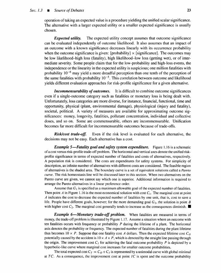
Example 5-Fatality goal and safety system expenditure. Figure 1.16 is a schematicof a cost versus risk-profile trade-off problem. The horizontal and vertical axes denote the unified risk-profile significance in terms of expected number of fatalities and costs of alternatives, respectively.A population risk is considered. The costs are expenditures for safety systems. For simplicity ofdescription, an infinite number of alternatives with different costs are considered. The feasible regionof alternatives is the shaded area. The boundary curve is a set of equivalent solutions called a Pareto
curve. The risk homeostasis line will be discussed later in this section. When two alternatives on thePareto curve are given, we cannot say which one is superior. Additional information is required toarrange the Pareto alternatives in a linear preference order.
Assume that G 1 is specified as a maximum allowable goal of the expected number of fatalities.Then point A in Figure 1.16 is the most economical solution with cost C1• The marginal cost at pointA indicates the cost to decrease the expected number of fatalities by one unit, that is, cost to save alife. People have different goals, however; for the more demanding goal Gz, the solution is point Bwith higher cost Cz. The marginal cost generally tends to increase as the consequences diminish.•
Example 6-Monetary trade-off problem. When fatalities are measured in terms ofmoney, the trade-off problem is illustrated by Figure 1.17. Assume a situation where an outcome withten fatalities occurs with frequency or probability P during the lifetime of a plant. The horizontalaxis denotes the probability or frequency. The expected number of fatalities during the plant lifetimethus becomes lOx P. Suppose that one fatality cost A dollars. Then the expected lifetime cost Copotentially caused by the accident is lOx A x P, which is denoted by the straight line passing throughthe origin. The improvement cost C I for achieving the fatal outcome probability P is depicted by ahyperbolic-like curve where marginal cost increases for smaller outcome probabilities.
The total expected cost CT = Co +C I is represented by a unimodal curve with global minimalat TC. As a consequence, the improvement cost at point IC is spent and the outcome probability

24 Basic Risk Concepts • Chap. /
Feasible Region
UioocoU-5 C:2Ql
a:.~n;n;u,
Pareto Curve
/ / msk Homeostasis
H
AC1 1- - -f-- - - - - -"""+--
G2 G1
Expected Number of Fatalities
O l.----Jl.- ---Jl.- _
oFigure 1.16. Trade-off problem betweenfatalities and reduction cost.
Figure 1.17. Trade-off problem when fa-tality is measured by mone-tary loss.
Uioo
o
/ Expected Total Cost
<,Co =10APExpectedOutcomeCost
r: Improvement/ Cost. C,
Popt
Outcome Probability P
is determined. Point OC denotes the expected cost of the potential fatal outcome. The marginalimpro vement cost at point / C is equal to the slope lO x A of the straight line O-OC ofexpected fataloutcome cost. In other words , the optimal slope for the improvement cost is determined as the cost often fatalities . Theoretically, the safety investment increases so long as the marginal cost with respectto outcome likelihood P is smaller than the cost of ten fatalities. Obviously. the optimal investmentcost increases when either fatality cost A or outcome size (ten fatalities in this example) increases.
In actual situations, the plant may cause multiple outcomes with different numbers of fatalitie s.For such cases, a diagram similar to Figure 1.17 is obtained with the exception that the horizontal axisnow denotes the number of expected fatalities from all plant scenarios. The optimal marginal im-provement cost with respect to the number of expected fatalities (i.e., the marginal cost for decreasingone expected fatality) is equal to the cost of one fatality.

Sec. J.3 • Source ofDebates 25
The cost versus risk-level trade-offs in Figures 1.16 and 1.17 make sense if and only if thesystem yields riskandbenefits; if no benefit is perceived, thetrade-off problem is moot. •
Equity value concept. Difficult problems arise in quantifying life in terms of dol-lars, and an "equity value of saving lives" has been proposed rather than "putting a priceon human life" [5]. According to the equity value theory, an alternative that leads togreater expenditures per life saved than numerous other alternatives for saving lives isan inequitable commitment of society's resources that otherwise could have been usedto save a greater number of lives. We have to stop our efforts at a certain slope of therisk-cost diagram of Figure 1.16 for any system we investigate [12], even if our risk unitconsists of fatalities. This slope is the price we can pay for saving a life, that is, the equityvalue.
This theory is persuasive if the resources are centrally controlled and can be allocatedfor any purpose whatsoever. The theory becomes untenable when the resources are privatelyor separately owned: a utilitycompany would not spend their money to improveautomobilesafety; people in advanced countries spend money to save people from heart diseases, whilethey spend far less money to save people from starvation in Africa.
Risklcostlbenefit (ReB) trade-off. According to Starr [13],
theelectricity generation options of coal, nuclear power, and hydroelectricity have been com-pared astobenefits and risks, andbeen persuasively defended bytheir proponents. Inretrospect,the past decade has shown that the comparative risk perspective provided by such quantita-tive analysis has notbeen an important component of thepastdecisions to build any of theseplants. Historically, initial choices have been made on the basis of performance economicsandpolitical feasibility, even in the nuclear power program.
Many technologies start with emphases on their positive aspects-their merits orbenefits. After a while, possibly after a serious accident, people suddenly face the problemof choosing one of twoalternatives, that is, accepting or rejecting the technology. Ideally,butnot always, they are shown a risk profile of the alternative together with the benefits fromthe technology. Decision making of this type occurs daily at hospitals before or duringa surgical operation; the risk profile there would be a Farmer curve with the horizontalaxis denoting longevity loss or gain, while the vertical axis is an excess probability peroperation.
Figure 1.18 shows another schematic relation between benefit and risk. The higherthe benefit, the higher the risk. A typical example is a heart transplant versus an anticlottingdrug.
Figure 1.18. Schematic relation betweenbenefits and acceptablerisks.
IINot Acceptable
Acceptable
More Benefits
26 Basic Risk Concepts • Chap. J
Bounded rationality concept. Traditional decision-making theory makes four as-sumptions about decision makers.
1. They have a clearly defined utility value for each outcome.
2. They possess a clear and exhaustive view of the possible alternatives open to them.
3. They can create a risk profile for the future associated with each alternative.
4. They will choose between alternatives to maximize their expected utility.
However, flesh and blood decision making falls short of these Platonian assumptions.In short, human decision making is severely constrained by its keyhole view of the problemspace that is called "bounded rationality" by Simon [14]:
The capacity of the human mind for formulating and solving complex problemsis very smallcompared with the size of the problems whose solutionsare required for objectively rationalbehaviorin therealworld-or evenfora reasonable approximation of suchobjectiverationality.
The fundamental limitation in human information processing gives rise to "satisficing"behavior, that is, the tendency to settle for satisfactory rather than optimal courses of action.
Risk homeostasis. According to risk homeostasis theory [15], the solution withcost C2 in Figure 1.16 tends to move to point H as soon as a decision maker changes thegoal from G I to G2; the former risk level G I is thus revisited. The theory states that peoplehave tendencies to keep a constant risk level even if a safer solution is available. Whena curved freeway is straightened to prevent traffic accidents, drivers tend to increase theirspeed, and thus incur the same risk level as before.
1.3.4 Summary
Different viewpoints toward risk are held by the individual affected, the populationaffected, the public, companies, and regulatory agencies. Disagreements arising in therisk-assessment phase encompass outcome, causal scenario, population affected, and like-lihood, while in the risk-management phase disagreement exists in loss/gain classification,outcome significance, available alternatives, risk profile significances, risk/cost trade-off,and risk/cost/benefit trade-off.
The following factors make risk management difficult: 1) incommensurability ofoutcomes, 2) bounded rationality, and 3) risk homeostasis. An equity value guideline isproposed to give insight for the trade-off problem between monetary value and life.
1.4 RISK-AVERSION MECHANISMS
PRAM involves both objective and subjective aspects. A typical subjective aspect arisingin the risk-management phase is an instinctive attitude called risk aversion, which is intro-duced qualitatively in Section 1.4.1. Section 1.4.2 describes three attitudes toward monetaryoutcomes: risk aversion, risk seeking, and risk neutral. Section 1.4.3 shows that the mon-etary approach can fail in the face of fatalities. Section 1.4.4 deals with an explanationof postaccident overestimation of outcome severity and likelihood. Consistent Bayesianexplanations are given in Sections 1.4.5 and 1.4.6 with emphasis on a posteriori distribu-tion. A public confidence problem with respect to the PRAM methodology is described inSection 1.4.7.

Sec. 1.4 • Risk-Aversion Mechanisms
1.4.1 Risk Aversion
27
It is believed that people have an ambivalent attitude toward catastrophic outcomes;small stimuli distributed over time or space are ignored, while the sum of these stimuli,if exerted instantly and locally, cause a significant response. For instance, newspapersignore ten single-fatality accidents but not one accident with ten fatalities. In order to avoidworst-case potential scenarios, people or companies buy insurances and pay amounts thatare larger than the expected monetary loss. This attitude is called risk aversion.
One reason for the dispute about nuclear power lies in attitude toward risk. In spite ofthe high population risk, people pay less attention to automobile accidents, which cause morethan ten thousand fatalities every year, because these accidents occur in an incremental anddispersed manner; however, people react strongly to a commercial airline accident whereseveral hundred people die simultaneously. In addition to the individual- versus population-risk argument, the risk-aversive attitude is an unavoidable subject in the risk-managementfield.
1.4.2 Three Attitudes Toward Monetary Outcome
Risk-aversive, -neutral, and -seeking, People perceive the significance of moneydifferently; its significance or utility is not necessarily proportional to the amount. Fig-ure 1.19 shows three attitudes in terms of loss or value function curves: risk-aversive(convex), risk-seeking (concave), and risk-neutral (linear). For the loss function curves,the positive direction of the horizontal axis denotes more loss, and the negative directionmore gain; the vertical axis denotes the loss significance of money. Each point on themonotonously increasing loss significance curve O-B-C-L in the upper-left-comer graphdenotes a significance value for each insurance premium dollar spent, that is, a loss withoutuncertainty. The smaller the significance value, the lower the loss. Each point on the thirdquadrant curve, which is also monotonously increasing, denotes a significance value for adollar gain.
Convex significance curve. A convex curve sex) is defined mathematically by theinequality holding for all Xl, x2, and probability P.
(1.17)
Insurance premium loss versus expected loss. Figure 1.20 shows an example ofa convex significance curve sex). Consider the risk scenario as a lottery where XI and X2
amounts of money are lost with probability 1 - P and P, respectively. As summarizedin Table 1.6, the function on the left-hand side of the convex curve definition denotes thesignificance of the insurance premium PX2 + (1 - P)XI. This premium is equal to theexpected amount of monetary loss from the lottery. Term PS(X2) + (1 - P)S(XI) on theright-hand side is the expected significance when two significances S(Xl) and S(X2) forloss Xl and X2 occur with the same probabilities as in the lottery; thus the right-hand sidedenotes a significance value of the lottery itself. The convexity implies that the insurancepremium loss is preferred to the lottery.
Avoidance ofworse case. Because the insurance premium PX2 +(1 - P)XI is equalto the expected loss of the lottery, one of the losses (say X2) is greater than the premiumloss, indicating that the risk-averse attitude avoids the worse case X2 in the lottery; in otherwords, risk-averse people will pay the insurance premium to compensate for the potentially
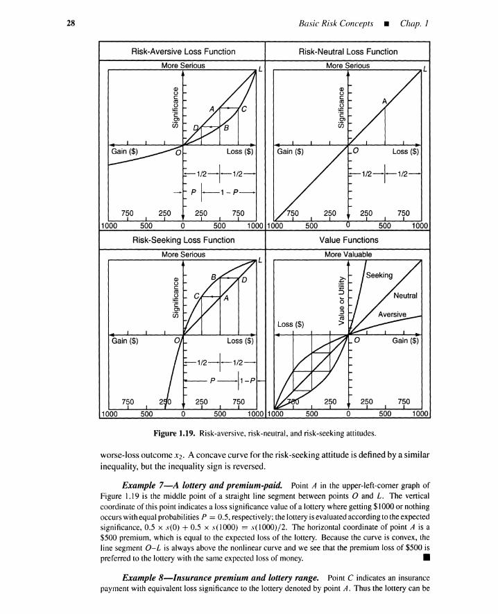
28
Risk-Aversive Loss Function
More Serious
Loss ($)
-1/2-1-1/2
p 1--1-P-750 250 250
1000 500 0 500
Risk-Seeking Loss Function
More Serious-------------------L
Basic Risk Concepts • Chap. 1
Risk-Neutral Loss Function
More Serious
1/2-1-1/2 -
Value Functions
More Valuable
Figure 1.19. Risk-aversive, risk-neutral, and risk-seeking attitudes.
worse-loss outcome X2. A concave curve for the risk-seeking attitude is defined by a similarinequality, but the inequality sign is reversed.
Example 7-A lottery and premium-paid. Point A in the upper-left-comer graph ofFigure 1.19 is the middle point of a straight line segment between points 0 and L. The verticalcoordinate of this point indicates a loss significancevalueof a lottery where getting $1000 or nothingoccurswithequal probabilities P = 0.5, respectively;the lotteryisevaluatedaccordingto theexpectedsignificance, 0.5 x s(O) + 0.5 x s(1000) = s( I000)/2. The horizontal coordinate of point A is a$500 premium, which is equal to the expected loss of the lottery. Because the curve is convex, theline segment O-L is always above the nonlinear curve and we see that the premium loss of $500 ispreferred to the lottery with the same expected loss of money. •
Example 8-lnsurance premium and lottery range. Point C indicates an insurancepayment with equivalent loss significance to the lottery denoted by point A. Thus the lottery can be
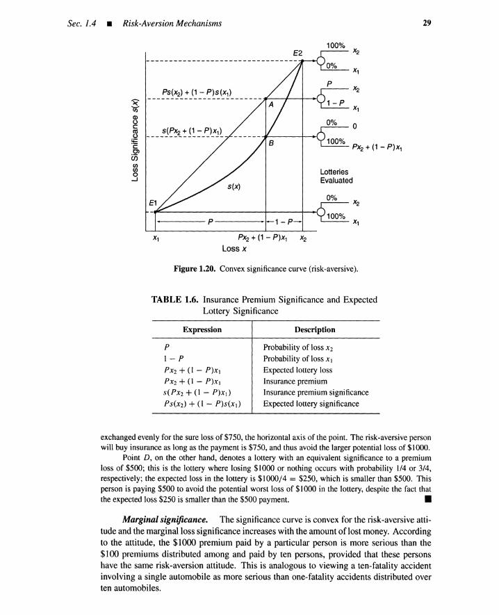
Sec. 1.4 • Risk-Aversion Mechanisms 29
100%X2
0%x,
PX2
1-P x,
0%0
100%PX2 + (1 - P)x,
100%
LotteriesEvaluated
~--x,,----- P-----""-1 - P-
S(PX2 + (1 - P)x,)-----------------
PS(X2) + (1 - P)s(x,)-------------------------4---~~~~')(
(;)Q)oc:Cd
~·20)
eneneno
...J
x, PX2 + (1 - P)x, X2
Loss x
Figure 1.20. Convex significance curve (risk-aversive).
TABLE 1.6. Insurance Premium Significance and ExpectedLottery Significance
Expression Description
P1- P
PX2+ (1 - P)XI
PX2+ (1 - P)Xl
S(PX2 + (1 - P)xd
PS(X2) + (1 - P)s(xd
Probability of loss X2
Probability of loss Xl
Expected lottery loss
Insurance premium
Insurance premium significance
Expected lottery significance
exchanged evenly for the sure loss of $750, the horizontal axis of the point. The risk-aversive personwill buy insurance as long as the payment is $750, and thus avoid the larger potential loss of $1000.
Point D, on the other hand, denotes a lottery with an equivalent significance to a premiumloss of $500; this is the lottery where losing $1000 or nothing occurs with probability 1/4 or 3/4,respectively; the expected loss in the lottery is $1000/4 = $250, which is smaller than $500. Thisperson is paying $500 to avoid the potential worst loss of $1000 in the lottery, despite the fact thatthe expected loss $250 is smaller than the $500 payment. •
Marginal significance. The significance curve is convex for the risk-aversive atti-tude and the marginal loss significance increases with the amount of lost money. Accordingto the attitude, the $1000 premium paid by a particular person is more serious than the$100 premiums distributed among and paid by ten persons, provided that these personshave the same risk-aversion attitude. This is analogous to viewing a ten-fatality accidentinvolving a single automobile as more serious than one-fatality accidents distributed overten automobiles.
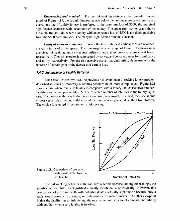
30 Basic Risk Concepts • Chap. J
Risk-seeking and -neutral. For the risk-seeking attitude in the lower-left-comergraph of Figure 1.19, the straight line segment is below the nonlinear concave significancecurve, and the fifty-fifty lottery is preferred to the premium loss of $500; the marginalsignificance decreases with the amount of lost money. The upper-right-comer graph showsa risk-neutral attitude, where a lottery with an expected loss of $500 is not distinguishablefrom the $500 premium loss. The marginal significance remains constant.
Utility ofmonetary outcome. When the horizontal and vertical axes are reversed,curves in terms of utility appear. The lower-right-comer graph of Figure 1.19 shows risk-aversive, risk-seeking, and risk-neutral utility curves that are concave, convex, and linear,respectively. The risk-aversion is represented by convex and concave curves for significanceand utility, respectively. For the risk-aversive curve, marginal utility decreases with theincrease of certain gain or the decrease of certain loss.
1.4.3 Significance ofFatality Outcome
When fatalities are involved, the previous risk-aversion and -seeking lottery problemdescribed in terms of monetary outcomes becomes much more complicated. Figure 1.21shows a case where one sure fatality is compared with a lottery that causes two and zerofatalities with equal probability 0.5. The expected number of fatalities in the lottery is justone. If a mother with two children is risk aversive, as is usually assumed, then she shouldchoose certain death of one child to avoid the more serious potential death of two children.The choice is reversed if the mother is risk seeking.
Figure 1.21. Comparison of one surefatality with 50% chance oftwo fatalities.
Q)oc:ctSo
't=·cen
Ci5CIJCIJo
...J
1
Numberof Fatalities2
The risk-seeking behavior is the intuitive outcome because, among other things, thesacrifice of one child is not justified ethically, emotionally, or rationally. However, thiscomparison of a certain death with potential deaths is totally sophomoric because only asadist would pose such a question, and only a masochist would answer it. Another viewpointis that the fatality has an infinite significance value, and we cannot compare one infinitywith another when a sure fatality is involveda
Sec. 1.4 • Risk-Aversion Mechanisms
1.4.4 Mechanisms forRisk Aversion
31
Overestimation offrequency and outcome. A more reasonable explanation of riskaversiveness for outcomes including fatalities was given by Bohnenblust and Schneider inSwitzerland [12]. According to them, misestimations of risks after severe accidents are oneof the major reasons for risk-aversive attitudes, which prefer ten single-fatality accidents toone accident with ten fatalities. Risks can be misestimated or overestimated with respectto size or likelihood of outcomes. This is similar to the error bands depicted in Figure 1.4,where the uncertainty is either due to errors of frequency or outcome severity estimation.
Overestimating outcome severity. Consider first the misestimation of an outcomeseverity such as the number of fatalities. Imagine a system that causes, on the average,one accident everyone hundred years. Most of these accidents have relatively small conse-quences, say one fatality for each. Once in a while there may be a catastrophic event withten fatalities. If the catastrophic event happens to occur, the public (or regulatory agen-cies) may believe that all accidents have catastrophic outcomes, thus they demand moresafety measures than are justified by the actual damage expectation. Such a claim is notrestricted to the particular facility that caused the accident; improvements are required forall other facilities of this type. As a consequence, all operators of this type of facility mustadopt a risk-averse behavior to avoid the excessive consequences caused by the one largeaccident.
Overestimation ofoutcome likelihood. Suppose that at a plant there is a one chancein ten thousand years for a serious accident. After the occurrence of such an accident,however, the public perception is no longer that the installation has an accident intervalof ten thousand years. The public might force the company to behave as if an accidentoccurred every thousand years, not every ten thousand years. This means that the risk andtherefore the safety costs are overestimated by a factor of ten.
Erosion ofpublic confidence. In the "Policy Statement on Safety Goals for theOperation of Nuclear Power Plants" published on August 4, 1986, the U.S. Nuclear Regula-tory Commission (NRC) recognizes that, apart from their health and safety consequences,severe core damage accidents can erode public confidence in the safety of nuclear power andcan lead to further instability and unpredictability for the industry. In order to avoid theseadverse consequences, the Commission intends to continue to pursue a regulatory programwith an objective of providing reasonable assurance, while giving appropriate considerationto the uncertainties involved [10].
1.4.5 Bayesian Explanation ofSeverity Overestimation
A priori distribution of defects. The public's and regulatory agencies' overesti-mation may not be a misestimation; it is consistent with a result from Bayesian statistics.*Assume that the accident occurs at a rate of once in one hundred years. Suppose that there isa debate about whether or not this type of facility poses a serious safety problem. The publicbelieves a priori that the existence and nonexistence of the defect are equally probable, thatis, P = 0.5; if the defect exists, the accident yields 10 fatalities with probability 0.99, and1 fatality with probability 0.01; if the defect does not exist, these probabilities are reversed.
*Theappendixof Chapter 3 describesthe Bayestheoremfor readers unfamiliarwith Bayesian statistics.
32 Basic Risk Concepts • Chap. J
A posteriori distribution ofdefects. Consider how the public belief about the defectchanges when the first accident yields ten fatalities. According to the Bayes theorem, wehave a posteriori probability of a defect conditioned by the occurrence of the ten-fatalityaccident.
Pr{Defect I 10} == Pr{Defect, 10}jPr{10} ==
Pr{Defect}Pr{ 10 I Defect}
Pr{Defect}Pr{ 10 I Defect} + Pr{No defect}Pr{ 10 I No defect}
0.5 x 0.99-------- == 0.990.5 x 0.99 + 0.5 x 0.01
(1.18)
(1.19)
(1.20)
Even if the first accident was simply bad luck, the public does not think that way;public belief is that in this type of facility the probability of a serious defect increasesto 0.99 from 0.5, yielding the belief that future accidents are almost certain to cause tenfatalities. An example is the Chemobyl nuclear accident. Experts alleviated the publicpostaccident shock by stating that the Chernobyl graphite reactor had a substantial defectthat U.S. reactors do not have.
Gaps between experts and public. It can be argued that the public a priori distri-bution
Pr{Defect} == Pr{No defect} == 0.5 (1.21 )
is questionable in view of the PRA that gives a far smaller a priori defect probability.However, such a claim will not be persuasive to the public that has little understandingof the PRA, and who places more emphasis on the a posteriori information after the realaccident, than on the a priori calculation before the accident. Spangler summarizes gapsin the treatment of technological risks by technical experts and the lay public, as given inTables 1.7 and 1.8 [5,16].
1.4.6 Bayesian Explanation ofLikelihood Overestimation
A priori frequency distribution. The likelihood overestimation can also be ex-plained by a Bayesian approach. Denote by F the frequency of the serious accident.Before the accident the public accepted the following a priori distribution of the frequency:Pr{F == 10-4
} == 0.99 and Pr{F == 10-2} == 0.01.
A posteriori distribution offrequency. Assume the first serious accident occurredafter one year's operation of the facility. Then the a posteriori distribution of the frequencyafter accident A is
Pr {F == 10-2 I A} == Pr{F == 10-2, A} IPr{ A} ==
Pr{F == 10-2}Pr{A I F = 10-2}----------------------- ==Pr{F = 10-2}Pr{A I F == 10-2} + Pr{F == 10-4}Pr{A I F == 10-4 }
0.01 x 0.01--------- ~ 0.5» 0.010.01 x 0.01 + 0.99 x 0.0001
(1.22)
(1.23)
(1.24)
An accident per one hundred years now becomes as plausible as an accident per tenthousand years. The public will not think that the first accident was simply bad luck.

Sec. 1.4 • Risk-Aversion Mechanisms
TABLE 1.7. Treatment of Technological Risks by Technical Experts
33
Approach
1. Criteria for risk acceptance
a. Absolutevs relativerisk
b. Risk-cost trade-offs
c. Risk-benefit comparisons of tech-nological options
d. Equityconsideration
2. Risk-assessment methods
a. Expression mode
b. Logic mode
c. Learningmode
3. Basis for trusting information
a. Sourcepreference
b. Source reliability
c. Accuracy of information
4. Risk-attribute evaluation
a. Low-frequency risk
b. Newnessof risk
c. Catastrophic vs disperseddeaths
d. Immediatevs delayed deaths
e. Statisticalvs knowndeaths
f. Dreadfulness of risk
g. Voluntary vs involuntary risk
5. Technological considerationa. Murphy's law (if anythingcan
go wrong, it will)
b. Reportsof technological failuresand accidents
Treatment Common to Experts
Riskjudged in both absoluteand relative terms
Essential to sound decision making because offinite societal resources for risk reduction andimpractability of achieving zero risk; tends toignore nondollar costs in such trade-offsEmphasizes total (net) benefits to society, neglect-ing benefits that are difficult to quantify; also ne-glects indirect and certain long-term benefits
Tends to treat shallowly withoutexplicit decisioncri-teria and structuredanalyses
Quantitative
Computational
• Risk = consequence x probability
• Fault trees/event trees
• StatisticalcalculationExperimental
• Laboratory animals• Clinicaldata for humans
• Engineering test equipmentand simulators
Establishedinstitutions
Qualification of experts
Robustness/uncertainty of scientific knowledge
Objective,conservative assessment
Broad range of high and low estimates
Givesequal weight
Diverse views over treatment of incommensurablesand discount rate
Givesequal weight
Generally ignores
Givesequal weight
Stimulus for redundancy and defense-in-depth insystem design and operating procedures; margins ofconservatism in design; quality assurance programsValued source of data for technological fixesand prioritizing research; increased attention toconsequence mitigation

34 Basic Risk Concepts • Chap. J
TABLE 1.8. Treatment of Technological Risks by Lay Public
Approach
1. Criteria for risk acceptance
a. Absolute vs relative risk
b. Risk-cost trade-offs
c. Risk-benefit comparisonsof tech-nological options
d. Equity consideration
2. Risk-assessmentmethods
a. Expression mode
b. Logic mode
c. Learning mode
3. Basis for trusting information
a. Source preference
b. Source reliability
c. Accuracy of information
4. Risk-attributeevaluation
a. Low-frequency risk
b. Newnessof risk
c. Catastrophic vs dispersed deaths
d. Immediate vs delayed deaths
e. Statistical vs knowndeaths
f. Dreadfulnessof risk
g. Voluntary vs involuntary risk
5. Technological consideration
a. Murphy's law (if anythingcango wrong, it will)
b. Reports of technological failuresand accidents
Treatment Common to the Public
Greater tendency to judge risk in absolute terms
Because human life is priceless, criteria involv-ing risk-cost trade-offs are immoral; ignoresrisks of no-action alternatives to rejected technol-ogy; gives greater weight to nondollar costs
Emphasizes personal rather than societal benefits;includes both qualitative and quantitative benefitsbut tends to neglect indirect and long-term benefits
Tends to distort equity considerations in favor ofpersonal interests to the neglect of the interests ofopposing parties or the common good of society
Qualitative
Intuitive
• Incompleterationale
• Emotional input to valuejudgments
Impressionistic
• Personal experience/memory
• Media accounts
• Cultural exchange
Nonestablishment sources
Limitedability to judge qualifications
Minimalunderstanding of strengthsand limitationsofscientificknowledge
Tends to exaggerateor ignore risk
Tends to exaggerateor ignore risk
Gives greater weight to catastrophicdeaths
Gives greater weight to immediate deaths except forknownexposure to cancer-producing agents
Gives greater weight to knowndeaths
Gives greater weight to dreaded risk
Gives greater weight to involuntary risk
Stimulus for what-if syndromes and distrust oftechnologies and technocrats; source of exaggeratedviews on risk levels using worst-case assumptions
Confirmsvalidityof Murphy's law; increaseddistrustof technocrats

Sec. 1.5 • Safety Goals
1.4.7 PRAM Credibility Problem
35
In Japan some people believe that the engineering approaches such as PRA are rela-tively useless for gaining public acceptance of risky facilities. Perhaps credibilities gainedby sharing a bottle of wine are more crucial to human relations. Clearly, the PRAM method-ology requires more psychosocial research to gain public credit.
According to Chauncey Starr of the Electric Power Research Institute [13]:
Science cannot prove safety, only the degree of existing harm. In the nuclear field emphasison PRA has focusedprofessional concernon the frequency of core melts. The arguments as towhetheracorecan meltwitha projectedprobability of onein a thousandperyear,or in a millionper year,representa misplacedemphasison thesequantitative outcomes. The virtueof the riskassessments is the disclosure of the system's causal relationships and feedback mechanisms,which might lead to technical improvements in the performance and reliabilityof the nuclearstations. When the probabilityof extremeevents becomesas small as these analysesindicate,the practical operating issue is the ability to manage and stop the long sequence of eventswhich could lead to extremeend results. Public acceptanceof any risk is more dependentonpublicconfidence in risk management than on the quantitative estimatesof risk consequences,probabilitiesand magnitudes.
1.4.8 Summary
Risk aversion is defined as the subjective attitude that prefers a fixed loss to a lotterywith the same amount of expected loss. When applied to monetary loss, risk aversionimplies convex significance curves, monotonously increasing marginal significance, andinsurance premiums larger than the expected loss. A risk-seeking or risk-neutral attitudecan be defined in similar ways. The comparison approach between the fixed loss andexpected loss, however, cannot apply to fatality losses.
Postaccident overestimation in outcome severity or in outcome frequency can beexplained by the Bayes theorem. The public places more emphasis on the a posterioridistribution after an accident than on the a priori PRA calculation.
1.5 SAFETY GOALS
When goals are given, risk problems become more tractable; risk management tries tosatisfy the goals, and the risk assessment checks the attainment of the goals. Goals for riskmanagement can be specified in terms of various measures including availability, reliability,risk, and safety. Aspects of these measures are clarified in Section 1.5.1. A hierarchicalarrangement of the goals is given in Section 1.5.2. Section 1.5.3 shows a three-layer decisionstructure with upper and lower bound goals. Examples of goals are given in Sections 1.5.4and 1.5.5 for normal activities and catastrophic accidents, respectively. Differences betweenidealistic and pragmatic lower bound goals are described in Section 1.5.6, where the conceptof regulatory cutoff level is introduced. The final section gives a model for varying theregulatory cutoff level as a function of population size.
1.5.1 Availability, Reliability, Risk, and Safety
Availability is defined as the characteristic of an item expressed by the probabilitythat it will be operational at a future instant in time (IEEE Standard 352). In this context, aprotection device such as a relief valve is designed to exhibit a high availability.

36 Basic Risk Concepts • Chap. J
Reliability is defined as a probability that an item will perform a required functionwhen used for its intended purpose, under the stated conditions, for a given period of time[4]. The availability is measured at an instant, and the reliability during a period of time.
Availability and reliability are independent of who is causing the loss outcome andwho is exposed to it. On the other hand, risk depends on the gain/loss assignment of theoutcome to people involved; shooting escaping soldiers is a gain for the guards, while beingshot is a loss for the escapees. Safety is only applicable to the people subject to the potentialloss outcome. That is, safety is originally a concept viewed from the aspect of people whoare exposed to the potential loss.
Fortunately, this subtle difference among availability, reliability, risk, and safety isusually irrelevant to PRAM where the people involved are supposed to be honest enoughto try to decrease potential losses to others. An alternative with less risk is thus consideredsafer; an instrument with a high availability or reliability is supposed to increase safety.Safety can thus be regarded as inversely proportional to the risk, and both terms are usedinterchangeably; it is, however, also possible for a company spending too much for safetyto face another risk: bankruptcy.
1.5.2 Hierarchical Goals forPRAM
Systems subject to PRA have a hierarchical structure: components, units, subsystems,plant, and site. Safety goals also form a hierarchy. For a nuclear power plant, for instance,goals can be structured in the following way [17] (see Figure 1.22):
1. Initiating event level: occurrence frequency
2. Safety system level: unavailability
3. Containment: failure probability
4. Accident sequence level: sequence frequency
5. Plant: damage frequency, source term
6. Site and environment: collective dose, early fatalities, latent cancer fatalities,property damage
The safety goals at the top of the hierarchy are most important. For the nuclear powerplant, the top goals are those on the site and environment level. When the goals on thetop level are given, goals on the lower levels can, in theory, be specified in an objectiveand systematic way. If a hierarchical goal system is established in advance, the PRAMprocess is simplified significantly; the probabilistic risk-assessment phase, given alterna-tives, calculates performance indices for the goals on various levels, with error bands. Therisk-management phase proposes the alternatives and evaluates the attainment of the goals.
To achieve goals on the various levels, a variety of techniques are proposed: suitableredundancy, reasonable isolation, sufficient diversity, sufficient independence, and suffi-cient margin [17]. Appendix A to Title 10 of the Code of Federal Regulations Part 50 (CFRPart 50) sets out 64 general design criteria for quality assurance; protection against fire,missiles, and natural phenomena; limitations on the sharing of systems; and other protectivesafety requirements. In addition to the NRC regulations, there are numerous supportingguidelines that contribute importantly to the achievement of safety goals. These includeregulatory guides (numbering in the hundreds); the Standard Review Plan for reactor li-cense applications, NUREG-75/087 (17 chapters); and associated technical positions andappendices in the Standard Review Plan [10].

Sec. J.5 • Safety Goals
Site and Environment
Early FatalitiesLatent Fatalities
Property DamagePopulation Exposure
I
Plant
Damage FrequencyReleased Material
IAccident Sequence
Frequency1
r I 1Initiating Safety Containment
Event System Barrier
Frequency Unavailability FailureProbability
Figure 1.22. Hierarchy of safetygoals.
1.5.3 Upper and Lower Bound Goals
37
Three-layer decision structure. Cyril Comar [18] proposed the following decisionstructure, as cited by Spangler [5]:
1. Eliminate any risk that carries no benefit or is easily avoided.
2. Eliminate any large risk ~ U that does not carry clearly overriding benefits.
3. Ignore for the time being any small risk S L that does not fall into category I.
4. Actively study risks falling between these limits, with the view that the risk oftaking any proposed action should be weighed against the risk of not taking thataction.
Of course , upper bound level U is greater than lower bound level L. The shaded areasin Figure 1.23 show acceptable risk regions with an elimination level L. The easily avoidedrisk in the first statement can, by definition, be reduced below L regardless of the merits .The term risk is used mainly to denote a risk level in terms of outcome likelihood. Theterm action in the fourth statement means an alternative ; thus action is not identical to a risksource such as a nuclear power plant or chemical plant; elimination of a particular actiondoes not necessarily imply elimination of the risk source; the risk source may continue toexist when other actions or alternatives are introduced.
In Comar's second statement, the large risk ~ U is reluctantly accepted if and onlyif it has overriding benefits such as risks incurred by soldiers at war (national security) orpatients undergoing operations (rescue from a serious disease) . Denote by R the risk levelof an action . Then the decision structure described above can be as stated in Figure 1.24.
We see that only risks with moderate benefits are subject to the main decision structure,which consists of three layers separated by upper and lower limits U and L, respectively:R ~ U,L < R < U,andR S L. In the top layer R ~ U,theriskisfirstreducedbelowU;

38 Basic Risk Concepts • Chap. I
No Moderate OverridingBenefit Benefits Benefits
Ben efit Leve l
BenefitsJustified
BenefitsNot
Justified..
:::J
Qi(ij0
> (9Q)
....J
.:£in -J
a: (ij0(9
Figure 1.23. Three-layer decision struc-ture.
Figure 1.24. Algorithm for three-layerdecision structure.
Prescreening Structure
beginif (risk carries no benefit)
reduce risk below L (inclusive);if (risk has overriding benefits)
reluctantly accept risk;if (risk has moderate benefits)
go to the main structure below;end
Ma in Decision Structure
r risk R has moderate benefits "lbeginif(R>= U )
risk is unacceptable;reduce risk below U (exclusive)
for justification or acceptance;if (L< R< U )
actively study risk for justification;beginif (risk is justified)
reluctantly accept risk;if (risk is not justified)
reduce risk until justifiedor below L (inclusive);
endif(R<= L)
accept risk;end
the resultant level may locate in the middle L < R < U or the bottom layer R ::: L. In themiddle layer, risk R is activelystudied by risk-cast-benefit (RC B) analyses for justification;if it is justified, then it is reluctantly accepted; if it is not justified, then it is reduced untiljustification in the middle layer or inclusion in the bottom layer. In the bottom layer, therisk is automatically accepted even if it carries no benefits.
Note that the term reduce does not necessarily mean an immediate reduction; ratherit denotes registration into a reduction list; some risks in the top layer or some risks not
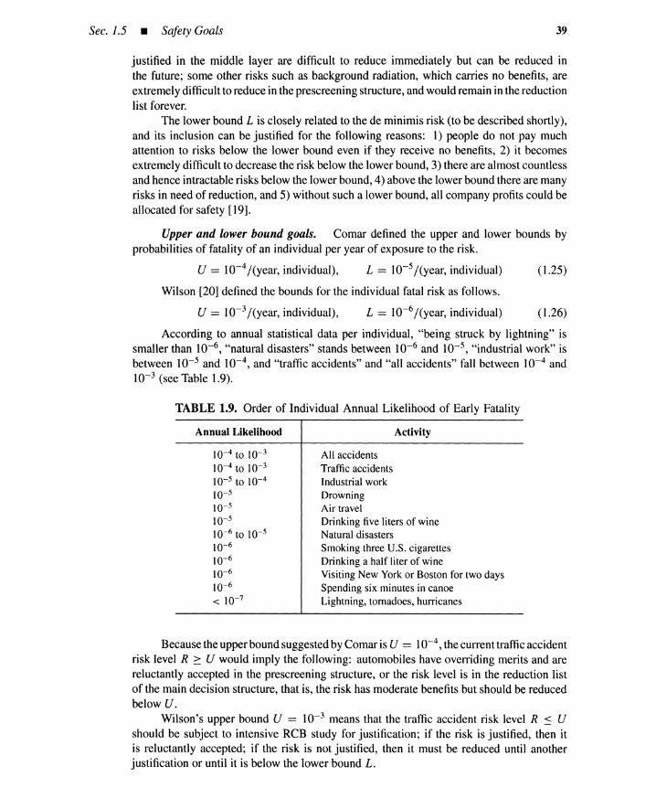
Sec. 1.5 • Safety Goals 39
justified in the middle layer are difficult to reduce immediately but can be reduced inthe future; some other risks such as background radiation, which carries no benefits, areextremely difficult to reduce in the prescreening structure, and would remain in the reductionlist forever.
The lower bound L is closely related to the de minimis risk (to be described shortly),and its inclusion can be justified for the following reasons: 1) people do not pay muchattention to risks below the lower bound even if they receive no benefits, 2) it becomesextremely difficult to decrease the risk below the lower bound, 3) there are almost countlessand hence intractable risks below the lower bound, 4) above the lower bound there are manyrisks in need of reduction, and 5) without such a lower bound, all company profits could beallocated for safety [19].
Upper and lower bound goals. Comar defined the upper and lower bounds byprobabilities of fatality of an individual per year of exposure to the risk.
U == 10-4/(year, individual), L == 10-5/(year, individual) (1.25)
Wilson [20] defined the bounds for the individual fatal risk as follows.
U == 10-3/(year, individual), L == 10-6/(year, individual) (1.26)
According to annual statistical data per individual, "being struck by lightning" issmaller than 10-6, "natural disasters" stands between 10-6 and 10-5, "industrial work" isbetween 10-5 and 10-4
, and "traffic accidents" and "all accidents" fall between 10-4 and10-3 (see Table 1.9).
TABLE 1.9. Order of Individual Annual Likelihood of Early Fatality
Annual Likelihood
10- 4 to 10- 3
10- 4 to 10- 3
10- 5 to 10- 4
10- 5
10-5
10-5
10-6 to 10- 5
10- 6
10- 6
10- 6
10-6
< 10- 7
Activity
All accidentsTraffic accidentsIndustrial workDrowningAir travelDrinking five liters of wineNatural disastersSmoking three U.S. cigarettesDrinking a half liter of wineVisiting New York or Boston for two daysSpending six minutes in canoeLightning, tornadoes, hurricanes
Because the upper bound suggested by Comar is U == 10-4, the current traffic accidentrisk level R 2: U would imply the following: automobiles have overriding merits and arereluctantly accepted in the prescreening structure, or the risk level is in the reduction listof the main decision structure, that is, the risk has moderate benefits but should be reducedbelow U.
Wilson's upper bound U == 10-3 means that the traffic accident risk level R :::: Ushould be subject to intensive RCB study for justification; if the risk is justified, then itis reluctantly accepted; if the risk is not justified, then it must be reduced until anotherjustification or until it is below the lower bound L.

40 Basic Risk Concepts • Chap. J
Wilson showed that the lower bound L == 10-6/(year, individual) is equivalent to therisk level of anyone of the following activities: smoking three U.S. cigarettes (cancer, heartdisease), drinking 0.5 liters of wine (cirrhosis of the liver), visiting New York or Boston fortwo days (air pollution), and spending six minutes in a canoe (accident). The lower boundL == 10-5 by Comar can be interpreted in a similar way; for instance, it is comparable todrinking five liters of wine per year.
Spangler claims that the Wilson's annual lower bound L == 10-6 is more acceptablethan Comar's bound L == 10-5 for the following situations [5]:
1. Whenever the risk is involuntary.
2. Whenever there is a substantial band of uncertainty in estimating risk at such lowlevels.
3. Whenever the risk has a high degree of expert and public controversy.
4. Whenever there is a reasonable prognosis that new safety information is morelikely to yield higher-than-current best estimates of the risk level rather than lowerestimates.
Accumulation problems for lower bound risks. The lower bound L == 10-6/(year,individual) would not be suitable if the risk level were measured not per year but peroperation. For instance, the same operation may be performed repetitively by a dangerousforging press. The operator of this machine may think that the risk per operation is negligiblebecause there is only one chance in one million of an accident, so he removes safetyinterlocks to speed up the operation. However, more than ten thousand operations may beperformed during a year, yielding a large annual risk level, say 10-2, of injury. Anothersimilar accumulation may be caused by multiple risk sources or by risk exposures to alarge population; if enough negligible doses are added together, the result may eventuallybe significant [11]; if negligible individual risks of fatality are integrated over a largepopulation, a sizable number of fatalities may occur.
ALARA-As low as reasonably achievable. A decision structure similar to theones described above is recommended by ICRP (International Commission on RadiologicalProtection) Report No. 26 for individual-related radiological protection [10]. Note thatpopulation-related protection is not considered.
1. Justification of practice: No practice shall be adopted unless its introduction pro-duces a positive net benefit.
2. Optimization of protection: All exposures shall be kept as low as reasonablyachievable (i.e., ALARA), economic and social factors being taken into account.
3. The radiation doses to individuals shall not exceed the dose equivalent limitsrecommended for the appropriate circumstances by ICRP.
The third statement corresponds to upper bound U in the three-layer decision structure.The ICRP report lacks lower bound L, however, and there is a theoretical chance that therisk would be overreduced to any small number, as long as it is feasible to do so by ALARA.
The NRC adoption of ALARA radiation protection standards for the design andoperation of light water reactors in May 1975 interpreted the term as low as reasonablyachievable to mean as low as is reasonably achievable taking into account the state oftechnology and the economics of improvements, in relation to benefits, to public health andsafety and other societal and socioeconomic considerations, and in relation to the utilizationof atomic energy in the public interest [10]. Note here that the term benefits does not denote
Sec. 1.5 • Safety Goals 41
the benefits of atomic energy but reduction of risk levels; utilizationofatomic energyin thepublic interestdenotes the benefits in the usual sense for RCB analyses.
For population-related protection, the NRC proposed a conservative value of $1000per total body person-rem (collective dose for population risk) averted for the risk/costevaluations for ALARA [10]. The value of $1000 is roughly equal to $7.4 million perfatality averted if one uses the ratio of 135 lifetime fatalities per million person-rems. ThisALARA value established temporarily by the commission is substantially higher than theequity value of $250,000 to $500,000 per fatality averted referenced by other agencies inrisk-reduction decisions. (The lower equity values apply, of course, to situations wherethere is no litigation, Le., to countries other than the United States.)
De minimis risk. The concept of de minimis risk is discussed in the book edited byWhipple [21]. A purpose of de minimis risk investigation is ajustification of a lower boundL below which no active study of the risk, including ALARA or RCB analyses, is required.Davis, for instance, describes in Chapter 13 of the book how the law has long recognizedthat there are trivial matters that need not concern it; the maxim de minimis non curat lex,"the law does not concern itself with trifles," expresses that principle [11]. (In practice, ofcourse, the instance of a judge actually dismissing a lawsuit on the basis of triviality is avery rare event.) She suggests the following applications of de minimis risk concepts [10].
1. For setting regulatory priorities
2. As a "floor" for ALARA considerations
3. As a cut-off level for collective dose assessments
4. For setting outer boundaries of geographical zones
5. As a floor for definition of low-level wastes
6. As a presumption of triviality in legal proceedings
7. To foster administrative and regulatory efficiency
8. To provide perspective for public understanding, including policy judgments
Some researchers of the de minimis say that 10-6/(year, individual) risk is trivial,acceptable, or negligible and that no more safety investment or regulation is required at allfor systems with the de minimis risk level. Two typical approaches for determining the deminimis radiation level are comparison with background radiation levels and detectabilityof radiation [11]. Radiation is presumed to cause cancers, and the radiation level can beconverted to a fatal cancer level.
ALARA versus de minimis. Cunningham [10] noted:
Wehave a regulatory scheme with upper limits abovewhich the calculatedhealth risk is gen-erally unacceptable. Below these upper limits are variousspecific provisionsand exemptionsinvolving calculatedrisks that are consideredacceptablebased on a balancingof benefits andcosts,andtheseneednotbeconsideredfurther. Regulatory requirements belowtheupperlimitsare based on the ALARAprinciple,and any risk involved is judged acceptablegiven not onlythe magnitudeof the healthrisk presentedbutalso varioussocialandeconomicconsiderations.A de minimis level,if adopted,wouldprovidea regulatory cutoff belowwhichany healthrisk,if present, could be considerednegligible. Thus, the de minimis level wouldestablish a lowerlimit for the ALARArange of doses.
The use of ALARA-type procedures can provide a basis for establishing an explicitstandard of de minimis risk beyond which no further analysis of costs and benefits needbe employed to determine the acceptability of risk [10]; in this context, the de minimis
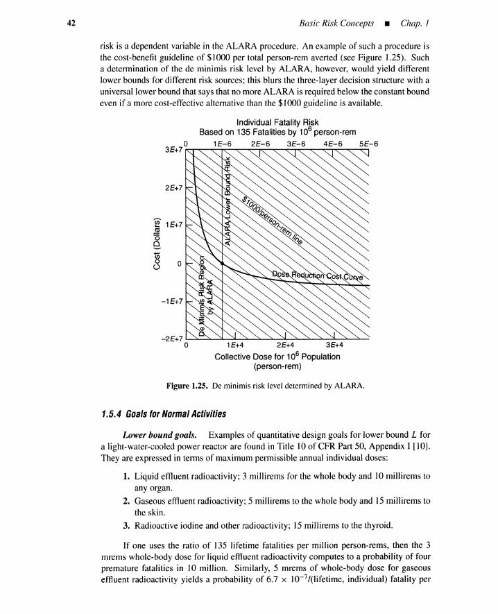
42 Basic Risk Concepts • Chap. 1
risk is a dependent variable in the ALARA procedure. An example of such a procedure isthe cost-benefit guideline of $1000 per total person-rem averted (see Figure 1.25). Sucha determination of the de minimis risk level by ALARA, however, would yield differentlower bounds for different risk sources; this blurs the three-layer decision structure with auniversal lower bound that says that no more ALARA is required below the constant boundeven if a more cost-effective alternative than the $1000 guideline is available.
1E+4 2E+4 3E+4
Collective Dose for 106 Population(person-rem)
o
-2E+7 L.--~~~--.-;a..~_~~--.llL----:O-~_~__--"""---"'-_
o
~ 1E+7~oe,(j)oo
-1E+7
Individual Fatality RiskBased on 135 Fatalities by 106 person-rem
o 1E-6 2E-6 3E-6 4E-6 5E-63E+7 ~~~~----':~~~~~--r"l:~~~~~---'::~
2E+7
Figure 1.25. De minimis risk level determined by ALARA.
1.5.4 Goals forNormal Activities
Lower bound goals. Examples of quantitative design goals for lower bound L fora light-water-cooled power reactor are found in Title 10 of CFR Part 50, Appendix I [10].They are expressed in terms of maximum permissible annual individual doses:
1. Liquid effluent radioactivity; 3 millirems for the whole body and 10 millirems toany organ.
2. Gaseous effluent radioactivity; 5 millirems to the whole body and 15 millirems tothe skin.
3. Radioactive iodine and other radioactivity; 15 millirems to the thyroid.
If one uses the ratio of 135 lifetime fatalities per million person-rems, then the 3mrems whole-body dose for liquid effluent radioactivity computes to a probability of fourpremature fatalities in 10 million. Similarly, 5 mrems of whole-body dose for gaseouseffluent radioactivity yields a probability of 6.7 x 10⁻⁷/(lifetime, individual) fatality per
Sec. 1.5 • Safety Goals 43
year of exposure. These values comply with the individual risk lower bound L == 10-6/(year,individual) proposed by Wilson or by the de minimis risk.
Upper bound goals. According to the current radiation dose rate standard, a maxi-mum allowable annual exposure to individuals in the general population is 500 mrems/year,excluding natural background and medical sources [1 I]. As a matter of fact, the averagenatural background in the United States is 100 mrem per year, and the highest is 310 mremper year. The 500 mrems/year standard yields a probability for a premature fatality of6.7 x 10-5 . This can be regarded as an upper bound V for an individual.
If the Wilson's bounds are used, the premature fatality likelihood lies in the middlelayer, L == 10-6 < 6.7 X 10⁻⁵ < V == 10-3. Thus the risk must be justified; otherwise,the risk should be reduced below the lower bound. A possibility is to reduce the risk belowthe maximum allowable exposure by using a safety-cost trade-off value such as the $1000person-rem in the NRC's ALARA concept [10].
A maximum allowable annual exposure to radiological industrial workers is 5 remsper year [11], which is much less stringent than for individuals in the general population.Thus we do have different upper bounds U's for different situations.
Having an upper bound goal as a necessary condition is better than nothing. Someunsafe alternatives are rejected as unacceptable; the chance of such a rejection is increasedby gradually decreasing the upper bound level. A similar goal for the upper bound hasbeen specified for N02 concentrations caused by automobiles and factories. Various upperbound goals have been proposed for risks posed by airplanes, ships, automobiles, buildings,medicines, food, and so forth.
1.5.5 Goals forCatastrophic Accidents
Lower bound goals. Some lower bound goals for catastrophic accidents are statedqualitatively. A typical example is the qualitative safety goals proposed by the NRC in1983 [22,10]. The first is related to individual risk, while the second is for population risk.
1. Individual risk: Individual members of the public should be provided a levelof protection from the consequences of nuclear power plant operation such thatindividuals bear no significant additional risk to life and health.
2. Population risk: Societal risks to life and health from nuclear power plant op-eration should be comparable to or less than the risks of generating electricity byviable competing technologies and should not be a significant addition to othersocietal risks.
The NRC proposal also includes quantitative design objectives (QDOs).
1. Prompt fatality QDO: The risk to an average individual in the vicinity of a nuclearpower plant of prompt fatalities that might result from reactor accidents shouldnot exceed one-tenth of one percent (0.1 percent) of the sum of prompt fatalityrisks resulting from other accidents to which members of the U.S. population aregenerally exposed.
2. Cancer fatality QDO: The risk to the population in the area near a nuclear powerplant of cancer fatalities that might result from nuclear power plant operationshould not exceed one-tenth of one percent (0.1 percent) of the sum of cancerfatality risks resulting from all other causes.
44 Basic Risk Concepts • Chap. J
3. Plant performance objective: The likelihood of a nuclear reactor accident thatresults in a large-scalecore melt should normally be less than ] in ]0,000 per yearof reactor operation.
4. Cost-benefit guideline: The benefit of an incremental reduction of societal mor-tality risks should be compared with the associatedcosts on the basis of $1000 perperson-rem averted.
The prompt (or accident) fatality rate from all causes in the United Statesin 1982 was 4 x 10- 4 per year; 93,000 deaths in a population of 231 million. At0.1% of this level, the prompt fatality QDO becomes 4 x 10- 7 per year, which issubstantially below the lower bound L == 10-6 for an individual [10]. In 1983,the rate of cancer fatalities was 1.9 x 10⁻³ . At 0.1% of this background rate, thesecond QDO is 1.9 x 10- 6 , which is less limiting than the lower bound.
On August 4, 1986, the NRC left unchanged the two proposed qualitativesafety goals (individual and population) and the two QDOs (prompt and cancer).It deleted the plant performance objective for the large-scale core melt. It alsodeleted the cost-benefit guideline. The following guideline was proposed forfurther examination:
5. General performance guideline: Consistentwiththe traditionaldefense-in-depthapproachand the accident mitigationphilosophyrequiringreliable performanceofcontainment systems, the overall mean frequency of a large release of radioactivematerials to the environment from a reactor accident should be less than 10-6 peryear of reactor operation.
The general performance guideline is also called an FP (fission products) large re-lease criteria. Offsite property damage and erosion of public confidence by accidents areconsidered in this criteria in addition to the prompt and cancer fatalities.
The International Atomic Energy Agency (IAEA) recommended other quantitativesafety targets in 1988 [23,24]:
1. For existing nuclear power plants, the probability of severe core damage shouldbe below 10-4 per plant operating year. The probability of large offsite releasesrequiring short-term responses should be below 10-5 per plant operating year.
2. For future plants, probabilities lower by a factor of ten should be achieved.
The future IAEA safety targets are comparable with the plant performance objectiveand the NRC general performance guideline.
Risk-aversion goals. Neither the NRC QDOs nor the IAEA safety targets considerrisk aversion explicitly in severe accidents; two accidents are treated equivalently if theyyield the same expected numbers of fatalities, even though one accident causes more fa-talities with a smaller likelihood. A Farmer curve version can be used to reflect the riskaversion. Figure 1.26 shows an example. It can be shown that a constant curve of expectednumber of fatalities is depicted by a straight line on a log j' versus log x graph, where x isthe number of fatalities and f is the frequency density around x.
Fatality excess curves have been proposed in the United States; more indirect curvessuch as dose excess havebeen proposed in other countries, although the latter can, in theory,be transformed into the former. The use of dose excess rather than fatality excess seems

Sec. 1.5 • Safety Goals
Figure 1.26. Constant fatality versusrisk-aversion goal in termsof Farmer curves.
s....i::''iiicQ)
o~cQ)::::l0-~
l.L
'0E-£.~
OJo
....J
10 100 1000
Logarithm of Number x of Fatalities
45
preferablein that it avoidsthe need to adopt a specific dose-riskcorrelation,to makeextrap-olations into areas of uncertainty, and to use upper limits rather than best estimates [11].
Risk profile obtained by cause-consequence diagram. Cause-consequence diagramswere invented at the RISIj> Laboratories in Denmark. This technology is a marriageof event trees (toshowconsequences) and fault trees (to showcauses), all takenin their naturalsequenceofoccurrence.Figure 1.27showsan example. Here,construction starts with the choice of a critical initiatingevent,motor overheating.
The block labeledA in the lowerleftof Figure 1.27is a compactwayof showingfaulttreesthatconsist of component failure events (motor failure, fuse failure, wiring failure, power failure), logicgates(OR, AND),and state-of-system events(motoroverheats,excessivecurrent to motor,excessivecurrent in circuit). An alternative representation (see Chapter4) of block A is given in Figure 1.28.
The consequencetracing part of the cause-consequence analysis involves taking the initiatingevent and following the resultingchain of events throughthe plant. At varioussteps, the chains maybranchinto multiplepaths. Forexample,the motoroverheating eventmayor may not lead to a motorcabinet local fire. The chains of events may take alternative forms, depending on conditions. Forexample,the progressof a firemay dependon whethera traffic jam prevents the firedepartment fromreaching the fire on time.
The procedurefor constructingthe consequence scenariois firstto take the initiatingeventandeach later event by asking:
1. Underwhat conditionsdoes this event lead to furtherevents?
2. What alternative plant conditions lead to differentevents?
3. Whatother components does the event affect? Does it affect more than one component?
4. What furtherevent does this event cause?
The cause tracingpart is represented by the fault tree. For instance,the event"motor overheat-ing" is tracedback to two pairsof concatenatedcauses: (fuse failure,wiringfailure) and (fuse failure,power failure).
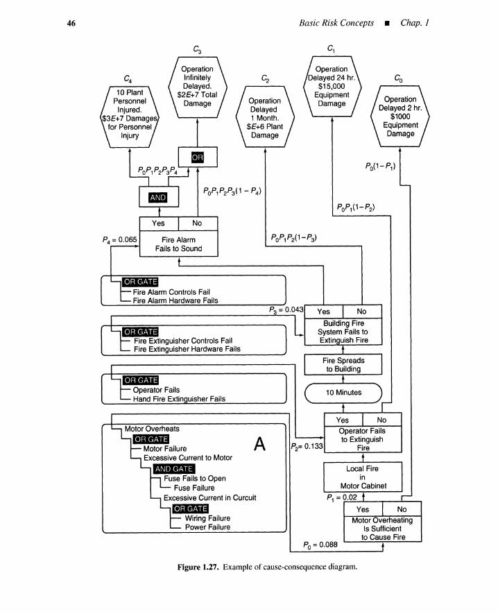
46 Basic Risk Concepts • Chap. J
P4 =0.065 Fire AlarmFails to Sound
Motor OverheatingIs Sufficient
to Cause Fire
Local Firein
Motor Cabinet
Operator Failsto Extinguish
Fire
Yes No
P1 = 0_.-02........---.------....Yes No
P2= 0.133'--__~po---_-.a
P3 = 0.043
AMotor Overheats
1·'i_l•Motor FailureExcessive Current to Motor
NII.&'IFuse Fails to Open
Fuse FailureExcessive Current in Curcuit
1·)i-14Wiring FailurePower Failure
1·]iIf41.Operator FailsHand Fire Extin uisher Fails
1.]jBn'I:!Fire Extinguisher Controls FailFire Extinguisher Hardware Fails
'.li_"Fire Alarm Controls FailFire Alarm Hardware Fails
Po =0.088
Figure 1.27. Exampleof cause-consequence diagram.
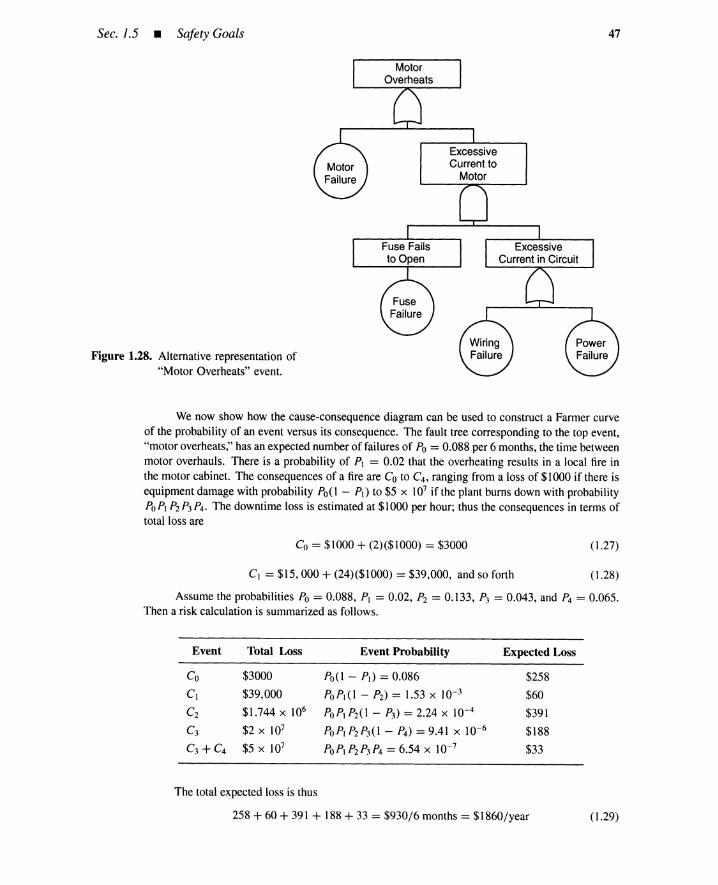
Sec. 1.5 • Safety Goals
Figure 1.28. Alternative representation of"Motor Overheats" event.
47
We now show how the cause-consequence diagram can be used to construct a Farmer curveof the probability of an event versus its consequence. The fault tree corresponding to the top event,"motor overheats," has an expected number of failures of Po = 0.088 per 6 months, the time betweenmotor overhauls. There is a probability of PI = 0.02 that the overheating results in a local fire inthe motor cabinet. The consequences of a fire are Co to C4 , ranging from a loss of $1000 if there isequipment damage with probability poe 1 - PI) to $5 x 10⁷ if the plant burns down with probabilityPo PI P2 P3 P4• The downtime loss is estimated at $1000 per hour; thus the consequences in terms oftotal loss are
Co = $1000 + (2)($1000) = $3000
CI = $15,000 + (24)($1000) = $39,000, and so forth
(1.27)
(1.28)
Assume the probabilities Po = 0.088, P, = 0.02, P2 = 0.133, P3 = 0.043, and P4 = 0.065.Then a risk calculation is summarized as follows.
Event Total Loss Event Probability Expected Loss
Co $3000 Po(1 - Pd = 0.086 $258
C I $39,000 POPt (1 - P2) = 1.53 x 10- 3 $60
C2 $1.744 x 10⁶ POPt P2( 1 - P3) = 2.24 x 10- 4 $391
C3 $2 x 10⁷ POPt P2 P3(1 - P4 ) = 9.41 x 10- 6 $188
C3 +C4 $5 X 10⁷ POPt P2P3 P4 = 6.54 X 10- 7 $33
The total expected loss is thus
258 + 60 + 391 + 188 + 33 = $930/6 months = $1860/year (1.29)
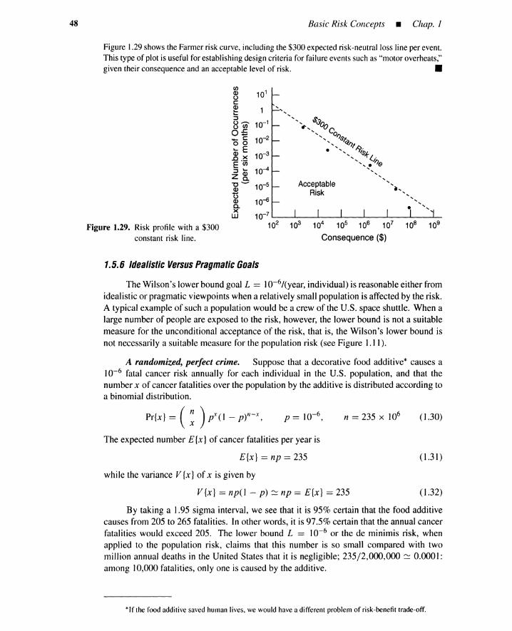
48 Basic Risk Concepts • Chap. J
Figure 1.29shows the Farmer risk curve, including the $300 expected risk-neutral loss line per event.This type of plot is useful for establishingdesign criteria for failureevents such as "motor overheats,"given their consequence and an acceptable level of risk. •
AcceptableRisk
104 105 106 107
Consequence($)Figure 1.29. Risk profile with a $300
constant risk line.
C/)Q)ocQ)~~
::J0-'oC/)O£~c00~ E~.~EC/)::J ~
z~"0"-'"Q)
t5Q)a.xw
10-5
10-6
10-7 '---_...a...-_-'---_--J.-_--'-_---'-_----l~_.L.._
102
1.5.6 Idealistic Versus Pragmatic Goals
The Wilson's lower bound goal L == 10-6/(year, individual) is reasonable either fromidealistic or pragmatic viewpoints when a relativelysmall population is affected by the risk.A typical example of such a population would be a crew of the U.S. space shuttle. When alarge number of people are exposed to the risk, however, the lower bound is not a suitablemeasure for the unconditional acceptance of the risk, that is, the Wilson's lower bound isnot necessarily a suitable measure for the population risk (see Figure 1.11).
A randomized, perfect crime. Suppose that a decorative food additive* causes a10-6 fatal cancer risk annually for each individual in the U.S. population, and that thenumber x of cancer fatalities over the population by the additive is distributed according toa binomial distribution.
Pr{x} = ( : ) pX(1 _ p)"-X,
The expected number E{x} of cancer fatalities per year is
E{x} == np == 235
while the variance V {x} of x is given by
n == 235 x 106 (1.30)
(1.31)
V{x} == np(l - p)::: np == E{x} == 235 (1.32)
By taking a 1.95 sigma interval, we see that it is 950/0 certain that the food additivecauses from 205 to 265 fatalities. In other words, it is 97.5% certain that the annual cancerfatalities would exceed 205. The lower bound L == 10-6 or the de minimis risk, whenapplied to the population risk, claims that this number is so small compared with twomillion annual deaths in the United States that it is negligible; 235/2,000,000 ::: 0.0001:among 10,000 fatalities, only one is caused by the additive.
*If the food additive saved human lives, we would have a different problem of risk-benefit trade-off.

Sec. J.5 • Safety Goals 49
In the de minimis theory, the size of the population at risk does not explicitly influencethe selection of the level of the lower bound risk. Indeed, the argument has been made thatit should not be a factor. The rationale for ignoring the size (or density) of the populationat risk when setting standards should be examined in light of the rhetorical question posedby Milvy [3]:
Why should the degree of protection that a person is entitled to differ according to how manyneighbors he or she has? Why is it all right to expose people in lightly populated areas to higherrisks than people in densely populated ones?
As a matter of fact, individual risk is viewed from the vantage point of a particularindividual exposed; if the ratio of potential fatalities to the size of the population remains aconstant, then the individual risk remains at the same level even if the population becomeslarger and the potential fatalities increase. On the other hand, population risk is a view froma risk source or a society that is sensitive to the increase of fatalities.
Criminal murders, in any country, are crimes. The difference between the 205 foodadditive murders and criminal murders is that the former are performed statistically. Acriminal murder requires that two conditions hold: intentional action to murder and evidenceof causal relations between the action and the death. For the food additive case, the firstcondition holds with a statistical confidence level of97.5%. However, the second conditiondoes not hold because the causal relation is probabilistic-l in 10,000 deaths in the UnitedStates. The 205 probabilistic deaths are the result of a perfect crime.
Let us now consider the hypothetical progress of a criminal investigation. Assumethat the fatal effects of the food additive can be individually traced by autopsy. Then thefood company using the additive would have to assume responsibility for the 205 cancerfatalities per year: there could even be a criminal prosecution. We see that for the foodadditive case there is no such concept as de minimis risk, acceptable risk level, or negligiblelevel of risk unless the total number of fatalities caused by the food additive is made muchsmaller than 205.
Necessity versus sufficiencyproblem. A risk from an alternative is rejected whenit exceeds the upper bound level U, which is all right because the upper bound goal is onlya necessary condition for safety. Alternatives satisfying this upper bound goal would not beaccepted if they neither satisfied the lower bound goal nor were justified by ReB analyses orALARA. A risk level is subject to justification processes when it exceeds the lower boundlevel L, which is also all right because the lower bound goal is also regarded as a necessarycondition for exemption from justification.
Many people in the PRA field, however, incorrectly think that considerably higherlower bound goals and even upper bound goals constitute sufficient conditions. They assumethat safety goals are solutions for problems of how safe is safe enough, acceptable levelof risks, and so forth. This failure to recognize the necessity feature of the lower andupper bound goals has caused confusion in PRA interpretations, especially for populationrisks.
Regulatorycutofflevel. An individual risk of 10-6/(year, individual) is sufficientlyclose to the idealistic, Platonic, lower bound sufficiency condition, that is, the de minimisrisk. Such a risk level, however, is far from idealistic for risks to large populations. Thelower bound L as a de minimis level for population risks must be a sufficiently smallfractional number; less than one death in the entire population per year. If some risk levelgreater than this de minimis level is adopted as a lower bound, the reason must come fromfactors outside the risk itself. A pragmatic lower bound is called a regulatory cutoff level.

50 Basic Risk Concepts • Chap. J
A pragmatic cutoff level is, in concept, different from the de minimis level: 1) theregulatory cutoff level is a level at or below which there are no regulatory concerns, and 2) ade minimis level is the lower bound level L at or below which the risks are accepted uncon-ditionally. Some risks below the regulatory cutoff level may not be acceptable, althoughthe risks are not regulated-the risks are only reluctantly accepted as a necessary evil. Con-sequently, the de minimis level for the population risk is smaller than the regulatory cutofflevel currently enforced.
Containment structures with IOO-foot-thick walls, population exclusion zones of hun-dreds of square miles, dozens of standby diesel generators for auxiliary feedwater sys-tems, and so on are avoided by regulatory cutoff levels implicitly involving cost consider-ations [IS].
Milvy [3] claims that a 10-6 lifetime risk to the U.S. population is a realistic andprudent regulatory cutoff level for the population risk. This implies 236 additional deathsover a 70-year interval (lifetime), and 3.4 deaths per year in the population of 236 million.This section briefly overviews a risk-population model as the regulatory cutoff level forchemical carcinogens.
Constant likelihood model. When the regulatory cutoff level is applied to an indi-vidual, or a discrete factory, or a small community population that is uniquely at risk, itsconsequences become extreme. A myriad of society's essential activities would have tocease. Certainly the X-ray technician and the short-order cook exposed to benzopyrene inthe smoke from charcoal-broiled hamburgers are each at an individual cancer risk consider-ably higher than the lifetime risk of 10- 6 . Indeed, even the farmer in an agricultural societyis at a 10-3 to 10-4 lifetime risk of malignant melanoma from pursuing his trade in thesunlight. The 10- 6 lifetime criterion may be appropriate when the whole U.S. populationis at risk, but to enforce such a regulatory cutoff level when the exposed population is smallis not a realistic option. Thus the following equation for regulatory cutoff level L I is toostrict for a small population
L I == 10-6 /Iifetirne (1.33)
Constant fatality model. On the other hand, if a limit of 236 deaths is selected asthe criterion, the equation for cutoff level L 2 for a lifetime is
L2 == (236/x)/lifetime, x: population size (1.34)
This cutoff level is too risky for a small population size of several hundred.
Geometric mean model. We have seen that, for small populations, L I from theconstant likelihood model is too strict and that L 2 from the constant fatality model is toorisky. On the other hand, the two models give the same result for the whole U.S. population.Multiplying the two cutoff levels and taking the square root yields the following equation,which is based on a geometric mean of L I and L 2•
L == 0.0151JX (1.35)
Using the equation with x == 100, the lifetime risk for the individual is 1.5 x 10- 3
and the annual risk is 2.14 x 10- 5• This value is nearly equal to the lowest annual fataloccupational rate from accidents that occur in the finance, insurance, and real estate oc-cupational category. The geometric mean risk-population model plotted in Figure 1.30 isdeemed appropriate only for populations of 100 or more because empirical data suggestthat smaller populations are not really relevant in the real world, in which environmental

Sec. 1.5 • Safety Goals 51
and occupational carcinogens almost invariably expose groups of more than 100 people.Figure 1.31 views the geometric mean model from expected number of lifetime fatalitiesrather than lifetime fatality likelihood.
Fatal Accident Rate:- -White-Coliar Workers
'-2 =236/x
10-7~---,_---,-_--,-_-",--_-..a..-_,"""",--_..A.-.._a..-101 102 103 104 105 106 107 108 109
Population, x
.....,J
-0 10-2
oo~ 10-3(J)~
~ 10-4
E2 10-5
:::i
Figure 1.30. Regulatory cutoff levelfrom geometric mean risk-population model.
.. . . .Constant-Fatality Model u.s. Risk
. . . .. .. . ".." .. .. .. .. . .. .:. . . . . .. .. :. .. .. . .. .. .. ..:. .. .. .. .. .. .. ~ .. . .. .. .. .. .. >. .. .. .. . .. ".. " .. . .. .. .. .. ; .. .. .. .. . .. ... .. .. .. .. .. . ... .. .. .. .. . .. .... .. .. .. .. .. .. .... .. . .. .. .. .. .... .. .. .. .. .. .. .... . .. .. .. .. .. ..
••••••• •••••••••• ••••••• '\ ••••••• • ••••••• 1 ••••••• •••••••••• ••••••• 1 •••••••
103 r----------------------,
10-6~-----------------~1 101 102 103 104 105 106 107 108 109
Population Size, x
Figure 1.31. Geometric mean model viewed from lifetime fatalities.
Pastregulatory decisions. Figure 1.32 compares the proposed cutoff level L withthe historical data of regulatory decisions by the Environmental Protection Agency. Solidsquares represent chemicals actively under study for regulation. Open circles representthe decision not to regulate the chemicals. The solid triangles provide fatal accident rates
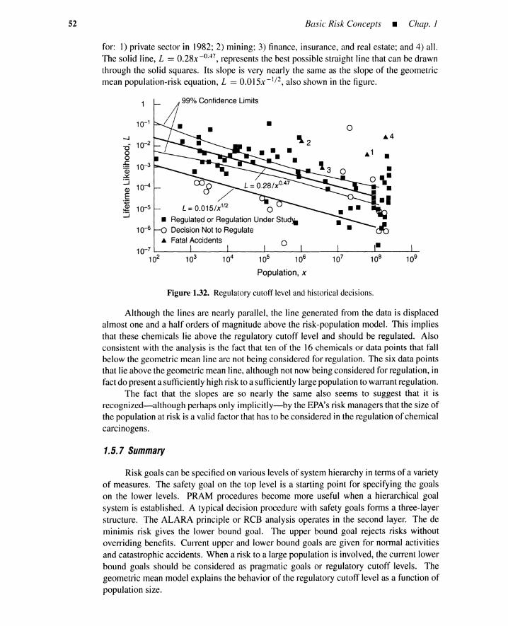
52 Basic Risk Concepts • Chap. J
for: 1) private sector in 1982; 2) mining; 3) finance, insurance, and real estate; and 4) all.The solid line, L == O.28x -0.47, represents the best possible straight line that can be drawnthrough the solid squares. Its slope is very nearly the same as the slope of the geometricmean population-risk equation, L == O.015x- I / 2, also shown in the figure.
10-1 • 0...,J 11 2
.4-0 10-2
0 .1 •0:f: 10-3CD •~ o ••::J
10-4 008 •Q) •E /~ 10-5 L =0.015/X1
/2
0::J
• Regulated or Regulation Under Stud~10-6 o Decision Not to Regulate
• Fatal Accidents10-7
102 103 104 105 106 107 108 109
Population, x
Figure 1.32. Regulatorycutoff level and historical decisions.
Although the lines are nearly parallel, the line generated from the data is displacedalmost one and a half orders of magnitude above the risk-population model. This impliesthat these chemicals lie above the regulatory cutoff level and should be regulated. Alsoconsistent with the analysis is the fact that ten of the 16 chemicals or data points that fallbelow the geometric mean line are not being considered for regulation. The six data pointsthat lie above the geometric mean line, although not now being considered for regulation, infact do present a sufficiently high risk to a sufficiently large population to warrant regulation.
The fact that the slopes are so nearly the same also seems to suggest that it isrecognized-although perhaps only implicitly-by the EPA's risk managers that the size ofthe population at risk is a valid factor that has to be considered in the regulation of chemicalcarcinogens.
1.5.7 Summary
Risk goals can be specified on various levels of system hierarchy in terms of a varietyof measures. The safety goal on the top level is a starting point for specifying the goalson the lower levels. PRAM procedures become more useful when a hierarchical goalsystem is established. A typical decision procedure with safety goals forms a three-layerstructure. The ALARA principle or RCB analysis operates in the second layer. The deminimis risk gives the lower bound goal. The upper bound goal rejects risks withoutoverriding benefits. Current upper and lower bound goals are given for normal activitiesand catastrophic accidents. When a risk to a large population is involved, the current lowerbound goals should be considered as pragmatic goals or regulatory cutoff levels. Thegeometric mean model explains the behavior of the regulatory cutoff level as a function ofpopulation size.
Chap. 1 • References
REFERENCES
53
[1] USNRC. "Reactor safety study: An assessment of accident risk in U.S. commercialnuclear power plants." USNRC, NUREG-75/014 (WASH-1400), 1975.
[2] Farmer, F. R. "Reactor safety and siting: A proposed risk criterion." Nuclear Safety,vo1.8,no.6,pp.539-548, 1967.
[3] Milvy, P. "De minimis risk and the integration of actual and perceived risks fromchemical carcinogens." In De Minimis Risk, edited by C. Whipple, ch. 7, pp. 75-86.New York: Plenum Press, 1987.
[4] USNRC. "PRA procedures guide: A guide to the performance of probabilistic riskassessments for nuclear power plants." USNRC, NUREG/CR-2300, 1983.
[5] Spangler, M. B. "Policy issues related to worst case risk analysis and the establishmentof acceptable standards of de minimis risk." In Uncertainty in Risk Assessment, RiskManagement, and Decision Making, pp. 1-26. New York: Plenum Press, 1987.
[6] Kletz, T. A. "Hazard analysis: A quantitative approach to safety." British Insititutionof Chemical Engineers Symposium, Sen, London, vol. 34,75,1971.
[7] Johnson, W. G. MORT Safety Assurance Systems. New York: Marcel Dekker, 1980.
[8] Lambert, H. E. "Case study on the use of PSA methods: Determining safety impor-tance of systems and components at nuclear power plants." IAEA, IAEA-TECDOC-590, 1991.
[9] Whipple, C. "Application of the de minimis concept in risk management." In DeMinimis Risk, edited by C. Whipple, ch. 3, pp. 15-25. New York: Plenum Press,1987.
[10] Spangler, M. B. "A summary perspective on NRC's implicit and explicit use of deminimis risk concepts in regulating for radiological protection in the nuclear fuelcycle." In De Minimis Risk, edited by C. Whipple, ch. 12, pp. 111-143. New York:Plenum Press, 1987.
[11] Davis, J. P. "The feasibility of establishing a de minimis level of radiation dose and aregulatory cutoffpolicy for nuclear regulation." In De Minimis Risk, edited by C. Whip-ple, ch. 13, pp. 145-206. New York: Plenum Press, 1987.
[12] Bohnenblust, H. and T. Schneider. "Risk appraisal: Can it be improved by formaldecision models?" In Uncertainty in Risk Assessment, Risk Management, and DecisionMaking, edited by V. T. Covello et al., pp. 71-87. New York: Plenum Press, 1987.
[13] Starr, C. "Risk management, assessment, and acceptability." In Uncertainty in RiskAssessment, Risk Management, and Decision Making, edited by V. T. Covello et al.,pp. 63-70. New York: Plenum Press, 1987.
[14] Reason, J. Human Error. New York: Cambridge University Press, 1990.
[15] Pitz, G. F. "Risk taking, design, and training." In Risk-Taking Behavior, edited byJ. F. Yates, ch. 10, pp. 283-320. New York: John Wiley & Sons, 1992.
[16] Spangler, M. "The role of interdisciplinary analysis in bringing the gap between thetechnical and human sides of risk assessment." Risk Analysis, vol. 2, no. 2, pp. 101-104, 1982.
[17] IAEA. "Case study on the use ofPSA methods: Backfitting decisions." IAEA, IAEA-TECDOC-591, April, 1991.
[18] Comar, C. "Risk: A pragmatic de minimis approach." In De Minimis Risk, edited byC. Whipple, pp. xiii-xiv. New York: Plenum Press, 1987.
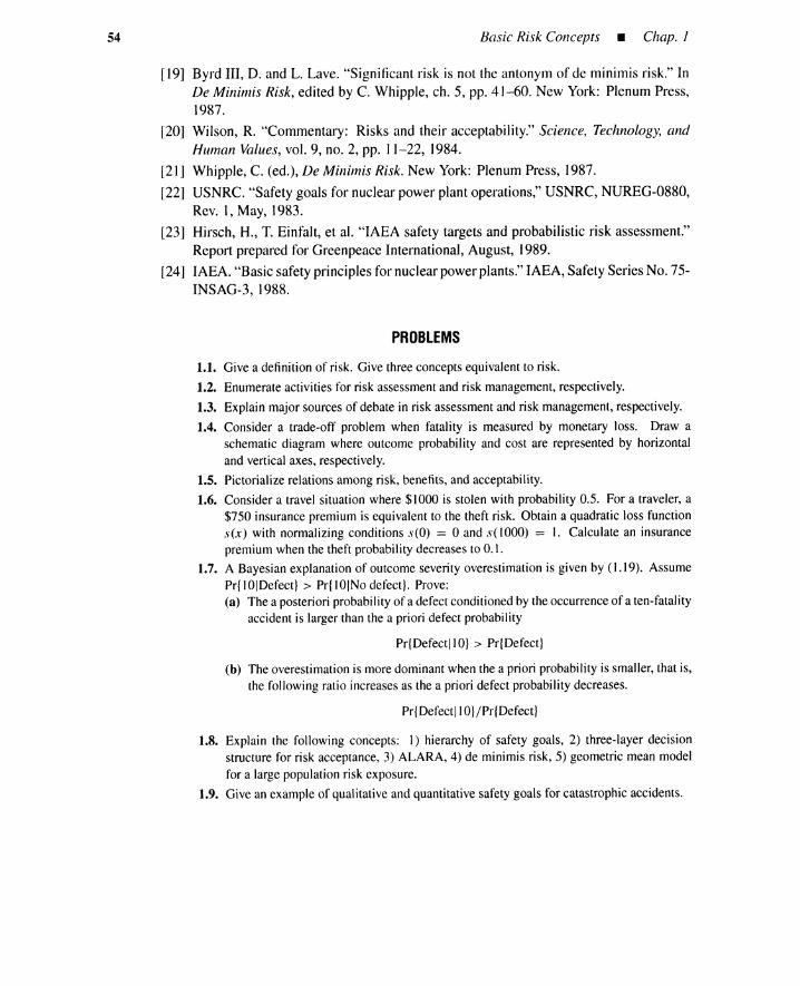
54 Basic Risk Concepts • Chap. J
[19] Byrd III, D. and L. Lave. "Significant risk is not the antonym of de minimis risk." InDe Minimis Risk, edited by C. Whipple, ch. 5, pp. 41-60. New York: Plenum Press,1987.
[20] Wilson, R. "Commentary: Risks and their acceptability." Science, Technology, andHuman Values, vol. 9, no. 2, pp. 11-22, 1984.
[21] Whipple, C. (ed.), De Minimis Risk. New York: Plenum Press, 1987.
[22] USNRC. "Safety goals for nuclear power plant operations," USNRC, NUREG-0880,Rev. 1, May, 1983.
[23] Hirsch, H., T. Einfalt, et al. "IAEA safety targets and probabilistic risk assessment."Report prepared for Greenpeace International, August, 1989.
[24] IAEA. "Basic safety principles for nuclearpower plants." IAEA, Safety Series No.7 5-INSAG-3, 1988.
PROBLEMS
1.1. Give a definition of risk. Give three concepts equivalent to risk.
1.2. Enumerate activities for risk assessment and risk management, respectively.
1.3. Explain major sources of debate in risk assessment and risk management, respectively.
1.4. Consider a trade-off problem when fatality is measured by monetary loss. Draw aschematic diagram where outcome probability and cost are represented by horizontaland verticalaxes, respectively.
1.5. Pictorialize relations among risk, benefits,and acceptability.
1.6. Consider a travel situation where $1000 is stolen with probability 0.5. For a traveler, a$750 insurance premium is equivalent to the theft risk. Obtain a quadratic loss functions(x) with normalizing conditions s(O) = a and s( 1000) = 1. Calculate an insurancepremium when the theft probabilitydecreases to 0.1.
1.7. A Bayesian explanation of outcome severity overestimation is given by (1.19). AssumePr{ la/Defect} > Pr{ 10lNodefect}. Prove:(a) The a posteriori probabilityof a defect conditioned by the occurrenceof a ten-fatality
accident is larger than the a priori defect probability
Pr{Defect/IO} > Pr{Defect}
(b) The overestimationis more dominant when the a priori probability is smaller, that is,the following ratio increases as the a priori defect probability decreases.
Pr{Defect/IO}/Pr{Defect}
1.8. Explain the following concepts: 1) hierarchy of safety goals, 2) three-layer decisionstructure for risk acceptance, 3) ALARA, 4) de minimis risk,S) geometric mean modelfor a large population risk exposure.
1.9. Give an example of qualitative and quantitativesafety goals for catastrophic accidents.

ccident Mechanismsand RiskManagement
2.1 INTRODUCTION
At first glance, hardware failures appear to be the dominant causes of accidents such asChemobyl, Challenger, Bhopal, and Three Mile Island. Few reliability analysts supportthis conjecture, however. Some emphasize human errors during operation, design, or main-tenance, others stress management and organizational factors as fundamental causes. Someemphasize a lack of safety culture or ethics as causes. This chapter discusses commonaccident-causing mechanisms.
To some, accidents appear inevitable because they occur in so many ways, but realityis more benign. The second half of this chapter presents a systematic risk-managementapproach for accident reduction.
2.2 ACCIDENT-CAUSING MECHANISMS
2.2.1 Common Features ofPlants with Risks
Features common to plants with potentially catastrophic consequences are physicalcontainment, stabilization of unstable phenomena, large size, new technology, componentvariety, complicated structure, large inertia, large consequence, and strict societal demandfor safety.
Physical containment. A plant is usually equipped with physical barriers or con-tainments to confine hazardous materials or shield hazardous effects. These containmentsare called physical barriers. For nuclear power plants, these barriers include fuel cladding,primary coolant boundary, and containment structure. For commercial airplanes, various
55
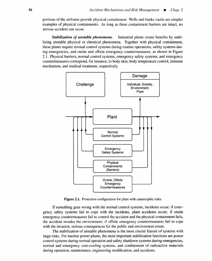
S6 Accident Mechanisms and Risk Management _ Chap. 2
portions of the airframe provide physical containment. Wells and banks vaults are simplerexamples of physical containments. As long as these containment barriers are intact, noserious accident can occur.
Stabilization of unstable phenomena. Industrial plants create benefits by stabi-lizing unstable physical or chemical phenomena. Together with physical containment,these plants require normal control systems during routine operations, safety systems dur-ing emergencies, and onsite and offsite emergency countermeasures, as shown in Figure2.1. Physical barriers, normal control systems, emergency safety systems, and emergencycountermeasurescorrespond, for instance, to body skin, body temperaturecontrol, immunemechanism, and medical treatment, respectively.
Damage
Challenge Individual, Society,Environment,
Plant
"
Plant
r" r"Normal
Control Systems
PhysicalContainments
(Barriers)
EmergencySafety Systems
1 _
Onsite,OffsiteEmergency
Countermeasures
Figure 2.1. Protection configuration for plant with catastrophic risks.
If something goes wrong with the normal control systems, incidents occur; if emer-gency safety systems fail to cope with the incidents, plant accidents occur; if onsiteemergency countermeasures fail to control the accident and the physical containment fails,the accident invades the environment; if offsite emergency countermeasures fail to copewith the invasion, serious consequences for the public and environmentensue.
The stabilization of unstable phenomena is the most crucial feature of systems withlarge risks. For nuclear power plants, the most important stabilization functions are powercontrol systems during normal operation and safety shutdownsystems during emergencies,normal and emergency core-cooling systems, and confinement of radioactive materialsduring operation, maintenance,engineering modification, and accidents.

Sec. 2.2 • Accident-Causing Mechanisms 57
Large size. Plants with catastrophic risks are frequently large in size. Examplesinclude commercial airplanes, space rockets and shuttles, space stations, chemical plants,metropolitan power networks, and nuclear power plants. These plants tend to be large forthe following reasons.
1. Economy of scale: Cost per product or service generally decreases with size. Thisis typical for ethylene plants in the chemical industry.
2. Demand satisfaction: Large commercial airplanes can better meet the demands ofair travel over great distances.
3. Amenity: Luxury features can be amortized over a larger economic base, that is,a swimming pool on a large ship.
New technology. Size increases require new technologies. The cockpit of a largecontemporary commercial airplane is as high as a three-story building. The pilots mustbe supported by new technologies such as autopilot systems and computerized displays tomaneuver the airplane for landing and takeoff. New technologies reduce airplane accidentsbut may introduce pitfalls during initial burn-in periods.
Component variety. A large number of system components of various types areused. Components include not only hardware but also human beings, computer programs,procedures, instructions, specifications, drawings, charts, and labels. Large-scale systemsconsist of millions of components. Failures of some components might initiate or enableevent propagations toward an accident. Human beings must perform tasks in this jungle ofhardware and software.
Complicated structure. A plant and its operating organization form a complicatedstructure with various lateral and vertical interactions. A composite hierarchy is formedthat encompasses the component, individual, unit, team, subsystem, department, facility,plant, corporation, and environment.
Inertia. An airplane cannot stop suddenly; it must remain in flight. A chemicalplant or a nuclear power plant requires a long time to achieve a quiescent state after initiationof a plant shutdown. A long period is also required for resuming plant operations.
Large consequence. An accident can have direct effects on individuals, society,environment, and plant and indirect effects on research and development, schedules, shareprices, public opposition, and company credibility.
Strict social demand for safety. Society demands that individual installations befar safer than, for example, automobiles, ski slopes, or amusement parks.
2.2.2 Negative Interactions Between Humans and the Plant
Human beings are responsible for the creation and improvement of plant safety andgain knowledge, abilities, and skills via daily operation. These are examples of positiveinteractions between human and plant. Unfortunately, as suggested by man-made accidents,most accidents are due to errors committed by humans [1]. It is thus necessary to investigatethe negative interactions between humans and plants.
Figure 2.2 shows these negative interactions when the plant consists of physicalcomponents such as hardware and software. The humans and the plant form an operatingorganization. This organization, enclosed by a general environment, is the risk-management
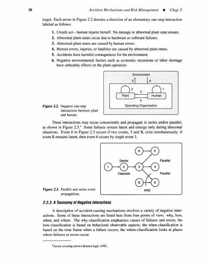
58 Accident Mechanisms and Risk Management _ Chap. 2
target. Each arrow in Figure 2.2 denotes a direction of an elementary one-step interactionlabeled as follows:
1. Unsafe act-human injures herself. No damage or abnormal plant state ensues.
2. Abnormal plant states occur due to hardware or software failures.
3. Abnormal plant states are caused by human errors.
4. Human errors, injuries, or fatalities are caused by abnormal plant states.
5. Accidents have harmful consequences for the environment.
6. Negative environmental factors such as economic recessions or labor shortagehave unhealthy effects on the plant operation.
Environment
Figure 2.2. Negative one-stepinteractions between plantand human.
5
plant)' ,[
6
Human )
These interactions may occur concurrently and propagate in series and/or parallel,as shown in Figure 2.3.* Some failures remain latent and emerge only during abnormalsituations. Event 6 in Figure 2.3 occurs if two events, 3 and B, exist simultaneously; ifevent B remains latent, then event 6 occurs by single event 3.
Series
0- 2
Cascade
Figure 2.3. Parallel and series eventpropagations.
2.2.3 ATaxonomy ofNegative Interactions
AND
Parallel
Parallel
A description of accident-causing mechanisms involves a variety of negative inter-actions. Some of these interactions are listed here from four points of view: why, how,when, and where. The why-classification emphasizes causes of failures and errors; thehow-classification is based on behavioral observable aspects; the when-classification isbased on the time frame when a failure occurs; the where-classification looks at placeswhere failures or errors occur.
•An arc crossingarrowsdenotes logic AND.

Sec. 2.2 • Accident-Causing Mechanisms
2.2.3.1 Why-Classification
59
Mechanical, functional, and interface failures. In mechanical failures, a devicebecomes unusable and fails to perform its function because some of its components fail.Forfunctional failures, a device is usable, but fails to perform its function because of causesnot attributable to the device or its components; a typical example is a perfect TV set whena TV station has a transmission problem. When devices interface, a failure of this interfaceis called an interface failure; this may cause a functional failure of one or two of the devicesinterfaced; a computer printer fails if its device driver has a bug.
Primary, secondary, and command failures. A primary failure is defined as thecomponent being in a nonworking state for which the component is held accountable, andrepair action on the component is required to return the component to the working state.A primary failure occurs under causes within the design envelope, and component naturalaging (wearout or random) is responsible for the failure. For example, "tank rupture due tometal fatigue" is a primary failure. The failure probability is usually time dependent.
A secondary failure is the same as a primary failure except that the component isnot held accountable for the failure. Past or present excessive stresses beyond the designenvelope are responsible for the secondary failure. These stresses involveout-of-toleranceconditions of amplitude, frequency, duration, or polarity, and energy inputs from thermal,mechanical, electrical, chemical, magnetic, or radioactiveenergy sources. The stresses arecaused by neighboring components or the environment, which includes meteorological orgeological conditions and other engineering systems.
Human beings such as operators and inspectors can cause secondary failures if theybreak component. Examples of secondary failures are "maintenance worker installs wrongcircuit breaker,""valve is damaged by earthquake," and "stray bullet cracks storage tank."Note that disappearance of the excessive stresses does not guarantee the working state ofthe component because the stresses have damaged the component that must be repaired.
A command failure is defined as the component being in a nonworking state due toimproper control signals or noise, and repair action is not required to return the componentto the working state; the component will function normally when a correct command isfed. Examples of command failures are "power is applied, inadvertently, to the relay coil,""switch fails to open because of electrical noise," "noisy input to safety monitor randomlygenerates spurious shutdown signals," and "operator fails to push panic button" (commandfailure for the panic button).
Secondary and command failures apply to human errors when the human is regardedas a device. Thus if an operator opens a valvebecause of an incorrect instruction, his failureis a command failure.
Basic and intermediatefailures. A basic failure is a lowest-level,highest resolutionfailure for which failure-rate (occurrence-likelihood)data are available. An example is amechanically stuck-closed failure of an electrical switch. Failures caused by a propagationof basic failures are called intermediate. An example is a lack of electricity caused bya switch failure. A primary or mechanical failure is usually considered a basic failure;occurrence-likelihooddata are often unavailablefor a secondary failure. When occurrencedata are guesstimated for secondary failures, these are treated as basic failures. Causesof command failure such as "area power failure" are also treated as basic failures whenoccurrence data are available.
60 Accident Mechanisms and Risk Management _ Chap. 2
Paralleland cascadefailures. Two or more failures may result from a single cause.This parallel or fanning-out propagation is called a parallel failure. Two or more failuresmay occur sequentially starting from a cause. This sequential or consecutive propagationis called a cascade or sequential failure. These propagations are shown in Figure 2.3. Anaccident scenario usually consists of a mixture of parallel and cascade failures.
Direct, indirect, and root causes. A direct cause is a cause most adjacent in timeto a device failure. A root cause is an origin of direct causes. Causes between a direct anda root cause are called indirect. Event 3 in Figure 2.3 is a direct cause of event 4; event 1is a root cause of event 4; event 2 is an indirect cause of event 4.
Main cause and supplemental causes. A failure may occur by simultaneous oc-currence of more than one cause. One cause is identified as a main cause, all others aresupplemental causes; event 3 in Figure 2.3 is a main cause of event 6 and event B is asupplemental cause.
Inducing factors. Some causes do not necessarily yield a device failure; they onlyincrease chances offailures. These causes are called inducingfactors. Smoking is an induc-ing factor for heart failure. Inducing factors are also called risk.factors. backgroundfactors,contributing factors, or shaping factors. Management and organizational deficiencies areregarded as inducing factors.
Hardware-induced, human-induced, and system-inducedfailures. This classifi-cation is based on what portions of a system trigger or facilitate failures. A human errorcaused by an erroneous indicator is hardware induced. Hardware failures caused by in-correct operations are human induced. Human and hardware failures caused by impropermanagement are termed system induced.
2.2.3.2 How-Classification
Random, wearout, and initial failures. A random failure occurs with a constantrate of occurrence; an example is an automobile water pump failing after 20,000 miles.A wearout failure occurs with an increasing rate of occurrence; an old automobile in abum-out period suffers from wearout failures. An initial failure occurs with a decreasingrate of occurrence; an example is a brand-new automobile failure in a bum-in period.
Demand and run failure. A demandfailure is a failure of a device to start or stopoperating when it receives a start or stop command; this failure is called a start or a stopfailure. An example is a diesel generator failing to start upon receipt of a start signal. Arun failure is one where a device fails to continue operating. A diesel generator failing tocontinue operating is a typical example of a run failure.
Persistent and intermittent failures. A persistent failure is one where a devicefailure continues once it has failed. For an intermittent failure, a failure only exists spo-radically. A relay may fail intermittently while closed. A typical cause of an intermittentfailure is electromagnetic circuit noise.
Active and latent failures. Active failures are felt almost immediately; as for latentfailures, their adverse consequences lie dormant, only becoming evident when they combinewith other factors to breach system defenses. Latent failures are most likely caused bydesigners, computer software, high-level decision makers, construction workers, managers,and maintenance personnel.

Sec. 2.2 • Accident-Causing Mechanisms 61
One characteristic of latent failures is that they do not immediately degrade a sys-tem, but in combination with other events-which may be active human errors or randomhardware failures-they cause catastrophic failure. Two categories of latent failures canbe identified: operational and organizational. Typical operational latent failures includemaintenance errors, which may make a critical system unavailable or leave the system in avulnerable state. Organizational latent failures include design errors, which yield intrinsi-cally unsafe systems, and management or policy errors, which create conditions inducingactive human errors. The latent failure concept is discussed more fully in Reason [1] andWagenaar et al. [2].
Omission and commission errors. When a necessary action is not performed, thisfailure is an omission error. An example is an operator forgetting to read a level indicatoror to manipulate a valve. A commission error is one where a necessary step is performed,but in an incorrect way.
Independent and dependentfailures. Failures A and B are independent when theproduct law of probability holds:
Pr{A and B} = Pr{A}Pr{B}
Failures are dependent if the probability of A depends on B, or vice versa:
Pr{A and B} # Pr{A}Pr{B}
(2.1)
(2.2)
Independent failures are sometimes called random failures; this is misleading becausefailures with a constant occurrence rate are also called random in some texts.
2.2.3.3 When-Classification
Recovery failure. Failure to return from an abnormal device state to a normal oneis called a recovery failure. This can occur after maintenance, test, or repair [3].
Initiating and enabling events. Initiating events cause system upsets that triggerresponses from the system's mitigative features. Enabling events cause failure of the sys-tem's mitigative features' ability to respond to initiating events; enabling events facilitateserious accidents, given occurrence of the initiating event [4].
Routine and cognitive errors. Errors in carrying out known, routine procedures arecalled routine or skill-based errors. Errors in thinking and nonroutine tasks are cognitiveerrors, which generate incorrect actions. A typical example of a cognitive error is an errorin diagnosis of a dangerous plant state.
Lapse, slip, and mistake. Suppose that specified, routine actions are known. Alapse is the failure to recall one of the required steps, that is, a lapse is an omission error. Aslip is a failure to correctly execute an action when it is recalled correctly. An example is adriver's inadvertently pushing a gas pedal when he intended to step on the brake. Lapses andslips are two types of routine errors. A mistake is a cognitive error, that is, it is a judgmentor analysis error.
2.2.3.4 Where-Classification
Internal and external events. An internal event occurs inside the system boundary,while an external event takes place outside the boundary. Typical examples of externalevents include earthquakes and area power failures.

62 Accident Mechanisms and Risk Management _ Chap. 2
Active andpassive failures. A device is called active when it functions by changingitsstate; anexample isanemergencyshutdownvalvethat is normallyopen. A devicewithouta state change is called passive; a pipe or a wire are typical examples. An active failure isan active device failure, while a passive failure is a passive device failure.
LOCA and transient. A LOCA (loss of coolant accident) is a breach in a coolantsystem that causes an uncontrollable loss of water. Transients are other abnormal conditionsof a plant that require that the plant be shut down temporarily [4]. A loss of offsite poweris an example of a transient. Another example is loss of feedwater to a steam generator. Acommon example is shutdown because of government regulatory action.
2.2.4 Chronological Distribution 01 Failures
Different types of failures occur at various chronological stages in the life of a plant.
1. Siting. A site is an area within which a plant is located [5]. Local characteristics,including natural factors and man-made hazards, can affect plant safety. Naturalfactors include geological and seismological characteristics and hydrological andmeteorological disturbances. Accidents take place due to an unsuitable plantlocation.
2. Design. This includes prototype design activities during research, development,and demonstration periods, and product or plant design. Design errors may becommitted during scaleup because of insufficientbudgets for pilot plant studies ortruncated research, development, and design. Keytechnologiessometimes remainblack boxes due to technology license contracts. Designers are given proprietarydata butdo not know where it came from. This can cause inadvertentdesign errors,especially when black boxes are used or modified and original specifications arehidden. Black box designs are the rule in the chemical industry where leased orrented process simulations are widely used.
In monitoring device recalls, the Food and Drug Administration (FDA) hascompiled data that show that from October 1983to November 1988approximately45% of all recalls were due to preproduction-related problems. These problemsindicate that deficiencies had been incorporated into the device design during apreproduction phase [6].
3. Manufacturing and construction. Defects may be introducedduring manufac-turingand construction; a plant could be fabricatedand constructed withdeviationsfrom original design specifications.
4. Validation. Errors indesign, manufacturing,andconstruction stages may persistafter plant validations that demonstrate that the plant is satisfactory for service. Asimple example of validation failures is a software package with bugs.
5. Operation. This is classified into normal operation, operationduring anticipatedabnormal occurrences, operation during complex events below the design basis,and operation during complex events beyond the design basis.(5·1) Normal operation. This stage refers to a period where no unusual chal-
lenge is posed to plant safety. The period includes start-up, steady-state,and shutdown. Normal operations include daily operation, maintenance,testing, inspection, and minor engineering modifications.

Sec. 2.2 • Accident-Causing Mechanisms 63
Tight operation schedules and instrumentation failures may induceoperator errors. Safety features may inadvertently be left nullified aftermaintenance because some valves may be incorrectly set; these types ofmaintenance failures typically constitute latent failures. Safety systems arefrequently intentionally disabled to avoid too many false alarms. Safetysystems become unavailable during a test interval.
(5·2) Anticipated abnormal occurrences. These occurrences are handled in astraightforward manner by appropriate control systems response as depictedin Figure 2.1. The term anticipated means such an event occurs more thanonce in a plant life. If normal control systems fail, anticipated abnormaloccurrences could develop into the complex events described below.
(5·3) Complex events below the design basis. System designers assume thathardware, software, and human failures are possible, and can lead to minorabnormal disturbances or highly unlikely accident sequences. Additionalprotection can be achieved by incorporating engineered features into theplant. These features consist of passive features such as physical barriersand active features such as emergency shutdown systems, standby electricgenerators, and water-tank systems.
Active systems are called engineered safety systems, and their per-formance is measured by on-demand performance and duration perfor-mance. The simplest forms of safety systems include circuit breakers andrupture disks. As shown in Figure 2.1, these safety features are required tosupplement protection afforded by normal control systems.
Design parameters of each engineered safety feature are defined byclassic, deterministic analyses that evaluate their effectiveness against com-plex events. The event in a spectrum of events that has the most ex-treme design parameters is used as the design basis. The engineeringsafety features are provided to halt progress of an undesirable event oc-curring below the design basis and, when necessary, to mitigate its conse-quences.
Safety features may fail to respond to complex events below the designbasis because something is wrong with the features themselves. High-stressconditions after a plant upset may induce human errors, and cause eventsthat occur below the design basis to propagate complex events beyond thedesign basis.
(5·4) Complex events beyond the design basis. Attention is directed to eventsof low likelihood but that are more severe than those explicitly considered inthe design. An event beyond the design basis can result in a severe accidentbecause some safety features have failed. For a chemical plant, these severeaccidents could cause a toxic release or a temperature excursion. These ac-cidents have a potential for major environmental consequences if chemicalmaterials are not adequately confined.
The classification of events into normal operation, anticipated abnor-mal occurrences, complex events below design basis, and complex eventsbeyond design basis is taken from IAEA No. 75-INSAG-3 [5]. It is usefulfor large nuclear power plants where it has been estimated that as much as
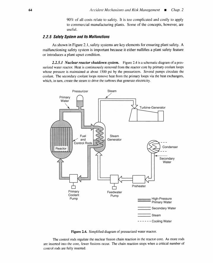
64 Accident Mechanisms and Risk Managemen t _ Chap. 2
90% of all costs relate to safety. It is too complicated and costly to applyto commercial manufacturing plants. Some of the concepts, however, areuseful.
2.2.5 Safety System and Its Malfunctions
As shown in Figure 2.1 , safety systems are key elements for ensuring plant safety. Amalfunctioning safety system is important because it either nullifies a plant safety featureor introduces a plant upset condition.
2.2.5.1 Nuclear reactor shutdown system. Figure 2.4 is a schematic diagramof a pres-surized water reactor. Heat is continuously removed from the reactor core by primary coolant loopswhose pressure is maintained at about 1500 psi by the pressurizers. Several pumps circulate thecoolant. The secondary coolant loops remove heat from the primary loops via the heat exchangers,which, in turn, create the steam to drive the turbines that generate electricity.
Pressur izer
PrimaryCoolantPump
Steam
/
SteamGenerator
FeedwaterPump
Turb ine-Generator
Condenser
SecondaryWater
[==:J High-PressurePrimary Water
___ Secondary Water
___ Steam
- - - - - - Cool ing Water
Figure 2.4. Simplified diagram of pressurized water reactor.
The control rods regulate the nuclear fission chain reaction in the reactor core. As more rodsare inserted into the core, fewer fissions occur. The chain reaction stops when a critical number ofcontrol rods are fully inserted.

Sec. 2.2 • Accident-Causing Mechanisms 65
Whenunsafeeventsin the reactorare detected,the shutdownsystemmustdrop enoughcontrolrods into the reactor to halt the chain reaction. This insertion is a reactor scram or reactor trip.The reactor monitoring system has sensors that continuously measure the following: neutron fluxdensity, coolant temperatureat the reactor core exit (outlet temperature), coolant temperature at thecore entrance (inlet temperature), coolant flow rate, coolant level in pressurizer, and on-off status ofcoolant pumps.
An inadvertentevent is defined as a deviation of a state variable from its normal trajectory.The simplest is an event where one of the measuredvariables goes out of a specified range. A morecomplicatedevent is a functionof one or more of the directly measuredvariables.
Figure 2.5 shows a diagram of a reactor shutdown system. Five features of the system arelisted.
1. Inadvertenteventsare monitoredby four identicalchannels,A, B, C, and D.
2. Each channel is physically independent of the others. For example, every channel has adedicatedsensor and a voting unit, a votingunit being definedas an action taken when mout of n sensorsgive identical indications.
3. Each channel has its own two-out-of-four:G voting logic. Capital G, standing for good,means that the logic can generate the trip signal if two or more sensors successfully detectan inadvertentevent. The logic unit in channel A has four inputs, XA, XB, Xc, XD, and oneoutput, TA • Input X A is a signal froma channelA sensor. This input is zero when the sensordetects no inadvertentevents, and unity when it senses one or more events. Inputs x B, Xc,
and xD are defined similarly. Note that a channel also receives sensor signals from otherchannels. Output TA representsa decision by the voting logic in channel A; zero valuesofTA indicate that the reactor should not be tripped; a value of I implies a reactor trip. Thevoting logic in channel B has the same inputs, XA, XB, xc, and XD, but it has output TB
specific to the channel. Similarly, channelsC and 0 have output Tc and TD, respectively.
4. A one-out-of-two:G twice logic with input TA , TB , Tc, and TD is used to initiate controlrod insertion, which is controlled by magnets energizedby two circuits. The two circuitsmust be cut off to deenergize the magnets; (TA , Tc) = (1, I), or (TA , TD ) = (1, I), or(TB , Tc ) = (1, 1), or (TB , TD) = (1, I). The rods are then released by the magnets anddropped into the reactorcore by gravity. •
2.2.5.2 Operating range and trip actions For nuclearpower plants, importantneutronand thermal-hydraulic variables are assigned operatingranges, trip setpoints,and safety limits. Thesafety limits are extreme valuesof the variables at which conservative analyses indicate undesirableor unacceptable damage to the plant. The trip setpointsare at lessextreme valuesof variables that, ifattained as a result of an anticipatedoperationaloccurrenceor an equipmentmalfunction or failure,would actuate an automaticplant protectiveaction such as a programmed power reduction, or plantshutdown. Trip setpoints are chosen such that plant variables will not reach safety limits. Theoperating range, which is the domain of normal operation, is bounded by values of variables lessextremethan the trip setpoints.
It is important that trip actions not be induced too frequently, especially when they are notrequired for protectionof the plant or public. A trip action could compromisesafety by sudden andprecipitouschanges,anditcouldinduceexcessivewearthatmightimpairsafetysystemsreliability[5].
Figure 2.6 showsa generalconfiguration of a safety system. The monitoringportion monitorsplant states; the judgment portion contains thresholdunits, votingunits, and other logic devices; theactuatorunit drives valves,alarms,and so on. Twotypes of failuresoccur in the safety system. •
2.2.5.3 Failed-Safe failure. The safety system is activated when no inadvertentevent exists and the system should not have been activated. A smoke detector false alarmor a reactor spurious trip is a typical failed-safe (FS) failure. It should be noted, however,that FS failures are not necessarily safe.
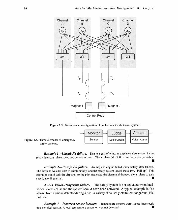
66 Accident Mechanisms and Risk Management • Chap. 2
ChannelA
ChannelB
Channe lC
ChannelD
Magnet 1 Magnet 2
Figure 2.5. Four-channel configuration of nuclear reactor shutdown system.
Figure 2.6. Three elements of emergencysafety systems.
-- Monitor - Judge I-- Actuate f--
Sensor Logic Circuit Valve, Alarm
Example I-Unsafe FS failure. Due to a gust of wind, an airplane safety system incor-rectly detects airplane speed and decreases thrust. The airplane falls 5000 m and very nearly crashes.
•Example 2-Unsafe FS failure. An airplane engine failed immediately after takeoff.
The airplane was not able to climb rapidly, and the safety system issued the alarm, "Pull up." Thisoperation could stall the airplane, so the pilot neglected the alarm and dropped the airplane to gainspeed, avoiding a stall. •
2.2.5.4 Failed-Dangerous failure. The safety system is not activated when inad-vertent events exist and the system should have been activated. A typical example is "noalarm" from a smoke detector during a fire. A variety of causes yield failed-d angerous (FD)failures.
Example I-Incorrect sensor location. Temperature sensors were spaced incorrectlyin a chemical reactor. A local temperature excursion was not detected. •
Sec. 2.2 • Accident-Causing Mechanisms 67
Example 2-Sensing secondaryinformation. Valve status was detected by monitoringan actuator signal to the valve. A mechanically stuck-closed failure was not detected because thevalve-open signal correctly reached the valve. •
Example 3-Sensorfailure.due to a seismic sensor biased low.
Train service incorrectly resumed after a severe earthquake
•Example 4-Excessive information load. A mainframe computer at a flood-warning
station crashed due to excessive information generated by a typhoon. •
Example 5-Sensor diversion. Sensors for normal operations were used for a safetysystem. A high temperature could not be detected because the normal sensors went out of range.Similar failures can occur if an inadvertent event is caused by sensor failures of plant controllers.•
Example 6-lnsufficient capacity. A large release of water from a safety water tankwashed poison materials into the Rhine due to insufficient capacity of the catchment basin. •
Example 7-Reputation. Malodorous gas generated by abnormal chemical reactions wasnot released to the environment because a company was nervous about lawsuits from neighbors. Thechemical plant exploded. •
Example 8-Too many alarms. At the Three Mile Island accident, alarm panels lookedlike Christmas trees, inducing operator errors, and eventually causing FO failures of safety systems .
•Example 9-Too little information. A pilot could not understand the alarms when his
airplane lost lift power. He could not cope with the situation. •
Example 10-1ntentional nullification. It has been charged that a scientist nullifiedvital safety systems to perform his experiment in the Chernobyl accident. •
Example l l-s-One-time activation. It is difficult to validate rupture disks and domesticfire extinguishers because they become useless once they are activated. •
Example 12-Simulated validation. Safety systems based on artificial intelligence tech-nologies are checked only for hypothetical accidents, not for real situations. •
2.2.6 Event Layer and Likelihood Layer
Given event trees and fault trees, various computer codes are available to calculateprobabilistic parameters for accident scenarios. However, risk assessment involves morethan a simple manipulation of probability formulas. Attention must be paid to evaluatingbasic occurrence probabilities used by these computer codes.
2.2.6.1 Event layer. Consider the event tree and fault tree in Figure 1.10. Weobserve that the tank rupture due to overpressure occurs if three events occur simultaneously:pump overrun, operator shutdown system failure, and pressure protection reliefvalve failure.The pump-overrun event occurs if either of two events occurs: timer contact fails to open,or timer itself fails. These causal relations described by the event and fault trees are on anevent layer level.
Event layer descriptions yield explicit causes of accident in terms of event occur-rences. These causes are hardware or software failures or human errors. Fault trees and theevent trees explicitly contain these failures. Failures are analyzed into their ultimate reso-lution by a fault-tree analysis and basic events are identified. However, these basic events
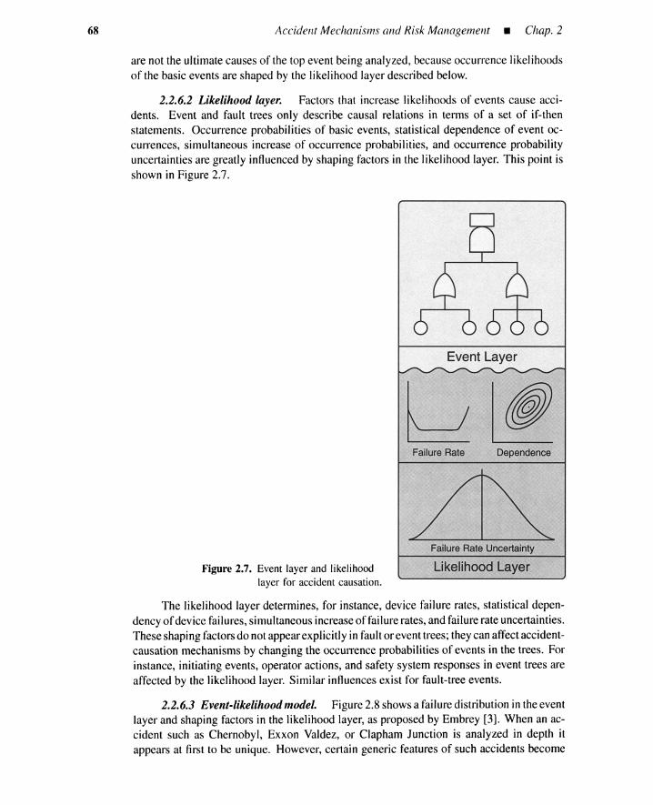
68 Accident Mechanisms and Risk Management _ Chap. 2
are not the ultimatecauses of the top event being analyzed, becauseoccurrence likelihoodsof the basic events are shaped by the likelihood layer described below.
2.2.6.2 Likelihood layer. Factors that increase likelihoods of events cause acci-dents. Event and fault trees only describe causal relations in terms of a set of if-thenstatements. Occurrence probabilities of basic events, statistical dependence of event oc-currences, simultaneous increase of occurrence probabilities, and occurrence probabilityuncertainties are greatly influencedby shaping factors in the likelihood layer. This point isshown in Figure 2.7.
Event Layer
Failure Rate Dependence
Figure 2.7. Event layer and likelihoodlayer for accident causation.
Failure Rate Uncertainty
Likelihood Layer
The likelihood layer determines, for instance, device failure rates, statistical depen-dencyof device failures, simultaneous increaseof failurerates,and failurerate uncertainties.These shaping factorsdo notappearexplicitly in faultor event trees; theycan affectaccident-causation mechanisms by changing the OCCUITence probabilitiesof events in the trees. Forinstance, initiating events, operator actions, and safety system responses in event trees areaffected by the likelihood layer. Similar influences exist for fault-treeevents.
2.2.6.3 Event-likelihood model. Figure 2.8showsa failuredistributionin theeventlayer and shaping factors in the likelihood layer, as proposed by Embrey [3]. When an ac-cident such as Chernobyl, Exxon Valdez, or Clapham Junction is analyzed in depth itappears at first to be unique. However, certain generic features of such accidents become
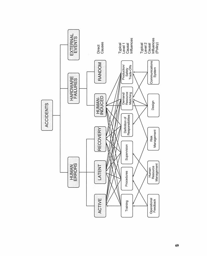
HUM
ANER
RO
RS
AC
CID
ENTS
HAR
DWAR
EFA
ILUR
ESEX
TERN
ALEV
ENTS
~ ~
ACTI
VE
Ope
ratio
nal
Fe
ed
ba
ck
LATE
NT
Hum
anR
esou
rce
Ma
na
ge
me
nt
REC
OV
ERY
Ris
kM
an
ag
em
en
t
HUM
AN-
INDU
CED
Des
ign
RAND
OM
Co
mm
un
ica
tion
sS
yste
m
Dire
ctC
ause
s
Typ
ical
Leve
l1
Cau
sal
Influ
ence
s
Typ
ical
Leve
l2C
ausa
lIn
fluen
ces
(Pol
icy)

70 Accident Mechanisms and Risk Management _ Chap. 2
apparent when a large number of cases are examined. Figure 2.8 is intended to indicate, ina simplified manner, how such a generic model might be represented. The generic modelis called MACHINE (model of accident causation using hierarchical influence networkelicitation). The direct causes, in the event layer, of all accidents are combinations ofhuman errors, hardware failures, and external events.
Human errors. Human errors are classified as active, latent, and recovery failures.The likelihoods of these failures are influenced by factors such as training, procedures, su-pervision, definition of responsibilities, demand/resource matching, and production/safetytrade-offs. These factors, in tum, are influenced by some of the higher-policy factors suchas operational feedback, human resource management, risk management, design, and com-munications system.
Hardware failures. Hardware failures can be categorized under two headings.Random (and wearout) failures are ordinary failures used in reliability models. Extensivedata are available on the distribution of such failures from test and other sources. Human-induced failures comprise two subcategories, those due to human actions in areas such asassembly, testing, and maintenance, and those due to inherent design errors that give riseto unpredicted failure modes or reduced life cycle.
As reliability engineers know, most failure rates for components derived from fielddata actually include contributions from human-induced failures. To this extent, such dataare not intrinsic properties of the components, but depend on human influences (manage-ment, organization) in systems where the components are employed.
External events. The third major class of direct causes is external events. Theseare characteristic of the environment in which the system operates. Such events are consid-ered to be independent of any human influence within the boundaries of the system beinganalyzed, although risk-management policy is expected to ensure that adequate defensesare available against external events that constitute significant threats to the system.
2.2.6.4 Event-tree analysis
Simple event tree. Consider the event tree in Figure 2.9, which includesan initiatingevent(IE), two operator actions, and two safety system responses [7]. In this oversimplified example,damage can be preventedonly if both operator actions are carried out correctly and both plant safetysystems function. The estimated frequency of damage (D) for this specific initiating event is
(2.3)
where .Ii) = frequency of damage (caused by this initiating event); .liE = frequency of the initiatingevent; Pi = probability of error of the ith operator action conditioned on prior events; and qiunavailabilityof the ith safety system conditioned on prior events.
Safety-system unavailability. Quality of organization and management should be re-flected in the parameters fIE, Pi, and qi. Denote by qi an average unavailabilityduring an intervalbetween periodic tests. The average unavailability is an approximation to time-dependent unavail-ability q., and is given by*
To 1qi = - + Y + Q+ -AT
T 2
*The time-dependent unavailability is fully described in Chapter 6.
(2.4)

Sec. 2.2 • Accident-Causing Mechanisms
Initiating Operator Safety Operator Safety StateEvent Action 1 System 1 Action 2 System 2
1 - q2OK1 - P2
q2 .----1 - q1
1 -P1 P2 Q)C>co
fiE q1 Ecoc
P1
"---
Figure 2.9. Simpleevent tree with two operatoractionsand two safetysystems.
71
where T = intervalbetweentests,To = durationof test,y = probabilityof failure due to testing,Q = probabilityof failure on demand,A = expectednumberof random failuresper unit time between tests.
Thus contributing to the averageunavailability are To/ T = test contribution while the safetysystem is disabledduring testing; y = human error in testing; Q = failure on demand; and ~ AT =randomfailuresbetweentests while the safety system is on standby.
Likelihood layer contributions. Asshownin Figure2.10,thesecontributions areaffectedby maintenance activities. These activities are, in turn, affected by the quality of all maintenanceprocedures. Qualityof variousproceduresis determinedby overallfactorssuchas safety knowledge,attitudetowardplant operationand maintenance, choiceof plant performancegoals, communication,responsibilities, and level of intelligenceand training. This figure is a simplified versionof the oneproposedby Wu,Apostolakis, and Okrent [7].
Safety knowledge. Safetyknowledge refersto everyonewho possessesknowledge of plantbehavior, severeaccidentconsequences, and related subjects,and whose combinedknowledge leadsto a total and pervasive safety ambiance.
Attitude. Uneventful, routine plant operation often makes the work environment boringrather than challenging. Plant personnelmay misinterpret stagnation for safety. A team with a slackand inattentiveattitude towardplant operationwill experiencedifficulty in bringingthe plant back tonormaloperationafter an abnormal occurrence.
Plant performance goal. Plant performancegoals are set by plant managers at a highorganizational level and influence plant personnel in making decisions during plant operation. Forexample, if an operatingteam constantlyreceivespressureand encouragementfrom high-level man-agers to achievehigh plant availability and to increasethe productionduring daily operations,opera-tors weighproductionconsequenceshigherthansafetyconsequences. Anotherextremeis a corporatepolicy that plant safety will help achieveefficiency and economy.
Communication and responsibility. It is not uncommon to find a situation where su-pervisors know operators sleep during their shifts but take no action (lack of responsibility). Somesupervisors do not have sufficient time to be in the plant to observe and supervise the efforts of theworkforce (lack of communication). Some companiestend to rely solely on writtencommunication
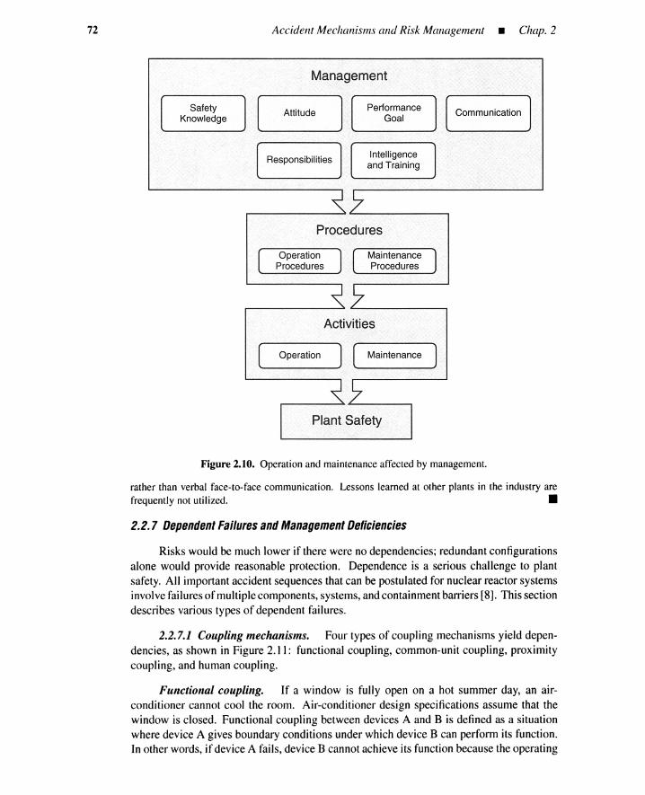
72 Accident Mechanisms and Risk Management _ Chap. 2
Management
Safety [ Attitude
1Performance I CommunicationKnowledge Goal
Responsibili ties Intelligenceand Training
~7Procedures
Operation MaintenanceProcedures Procedures
~~Activit ies
[ Operat ion ) [ Maintenance )
~7Plant Safety
Figure2.10. Operation and maintenance affected by management.
rather than verbal face-to-face communication. Lessons learned at other plants in the industry arefrequently not utilized. •
2.2.7 Dependent Failures and Management Deficiencies
Risks would be much lower if there were no dependencies; redundantconfigurationsalone would provide reasonable protection. Dependence is a serious challenge to plantsafety. All important accident sequences that can be postulated for nuclear reactor systemsinvolve failures of multiplecomponents,systems,andcontainmentbarriers[8]. This sectiondescribes various types of dependent failures.
2.2.7.1 Coupling mechanisms. Four types of coupling mechanisms yield depen-dencies, as shown in Figure 2.11 : functional coupling, common-unit coupling, proximitycoupling, and human coupling.
Functional coupling. If a window is fully open on a hot summer day, an air-conditioner cannot cool the room. Air-conditioner design specifications assume that thewindow is closed. Functional coupling between devices A and B is defined as a situationwhere device A gives boundaryconditions under which device B can perform its function.In other words, if device A fails, device B cannot achieve its function because the operating

Sec. 2.2 • Accident-Causing Mechanisms
« co « coQ) Q) Q)
CommonQ)
o Function o o o.S; .S; .S;Unit
os;Q) Q) Q) Q)
Cl c c c
73
«Q)o.S;Q)
c
Proximity
coQ)ooS;Q)
o
«Q)o.S;Q)
oHuman
coQ)o.S;Q)
c
Figure 2.11. Fourcouplingmechanisms of dependentfailures.
environment is outside the scope of device B's design specifications. Devices A and B failsequentially due to functional coupling.
An example is a case where systems A and B are a scram system and an emergencycore-cooling system (ECCS), respectively, for a nuclear power plant. Without terminatingchain reactions by insertion (scram) of control rods, the ECCS cannot achieve its func-tion even if it operates successfully. A dependency due to functional coupling is called afunctional dependency [8].
Common-unit coupling. Imagine a situation where devices A and B have a commonunit, for instance, a common power line. If the common unit fails, then the two devices failsimultaneously. This type of dependency is called a shared-equipment dependency [8].
Proximity coupling. Several devices may fail simultaneously because of proximity.Assume a floor plan with room numbers in Figure 2.12(a). Figures 2.12(b), (c), and (d)identify rooms influenced by five sources of impact, two sources of vibration, and twosources of temperature increase. Impact-susceptible devices in rooms 102 and 104 may faildue to impact source IMP-I.
The proximity coupling is activated either by external events or internal failures. Ex-ternal events usually result in severe environmental stresses on components and structures.Failures of one or more systems within a plant (internal failures) can create extreme en-vironmental stresses. For instance, sensors in one system might fail due to an excessivetemperature resulting from a second system's failure to cool a heat source [8]. The simulta-neous sensor failures are due to a proximity coupling triggered by a functional dependencyon the cooling system.
Human coupling. These are dependencies introduced by human activities, includ-ing errors of omission and commission. Persons involved can be anyone associated with aplant-life-cycle activity, including designers, manufacturers, constructors, inspectors, op-erators, and maintenance personnel. Such a dependency emerges, for example, when anoperator turns off a safety system when she fails to diagnose the plant condition-an event
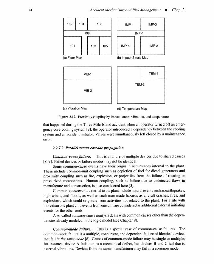
74 Accident Mechanisms and Risk Management _ Chap. 2
102 104 106
199
101 103 105
(a) Floor Plan
VIB-1
VIB-2
(c) Vibration Map
IMP-1 IMP-3
IMP-4
IMP-5 IMP-2
(b) Impact-Stress Map
TEM-1
TEM-2
(d) Temperature Map
Figure 2.12. Proximitycouplingby impact-stress, vibration, and temperature.
that happened during the Three Mile Island accident when an operator turned off an emer-gency core-cooling system [8]; the operator introduced a dependency between the coolingsystem and an accident initiator. Valves were simultaneously left closed by a maintenanceerror.
2.2.7.2 Parallel versus cascade propagation
Common-cause failure. This is a failure of multiple devices due to shared causes[8, 9]. Failed devices or failure modes may not be identical.
Some common-cause events have their origin in occurrences internal to the plant.These include common-unit coupling such as depletion of fuel for diesel generators andproximity coupling such as fire, explosion, or projectiles from the failure of rotating orpressurized components. Human coupling, such as failure due to undetected flaws inmanufacture and construction, is also considered here [5].
Common-cause events external to the plant include natural events such as earthquakes,high winds, and floods, as well as such man-made hazards as aircraft crashes, fires, andexplosions, which could originate from activities not related to the plant. For a site withmore than one plant unit, events from one unit are considered as additional external initiatingevents for the other units.
A so-called common-cause analysis deals with common causes other than the depen-dencies already modeled in the logic model (see Chapter 9).
Common-mode failure. This is a special case of common-cause failures. Thecommon-mode failure is a multiple, concurrent, and dependent failure of identical devicesthat fail in the same mode [8]. Causes of common-mode failure may be single or multiple;for instance, device A fails due to a mechanical defect, but devices Band C fail due toexternal vibrations. Devices from the same manufacturer may fail in a common mode.

Sec. 2.3 • Risk Management 75
Propagating failure. This occurs when equipment fails in a mode that causessufficient changes in operating conditions, environment, or requirements to cause otheritems of equipment to fail. The propagating failure (cascade propagation) is a way ofcausing common-cause failures (parallel propagation).
2.2.7.3 Management deficiency dependencies. Dependent-failure studies usuallyassume that multiple failures occur within a short time interval, and that components affectedare of the same type. Organizational and managerial deficiencies, on the other hand, canaffect various components during long time intervals. They not only introduce dependenciesbetween failure occurrences but also increase occurrence probabilities [7].
2.2.8 Summary
Features common to plants with catastrophic risks are presented: confinement byphysical containment and stabilization ofunstable phenomena are important features. Theseplants are protected by physical barriers, normal control systems, emergency safety systems,and onsite and offsite emergency countermeasures.
Various failures, errors, and events occur in hazardous plants, and these are seen asseries and parallel interactions between humans and plant. Some of these interactions arelisted from the points of view of why, how, when, and where. It is emphasized that thesenegative interactions occur during any time in the plant's life: siting, design, manufactur-ing/construction, validation, and operation. The plant operation period is divided into fourphases: normal operation, anticipated abnormal occurrences, complex events below thedesign basis, and complex events beyond the design basis.
A nuclear reactor shutdown system is presented to illustrate emergency safety systemsthat operate when plant states reach trip setpoints below safety limits, but above the operatingrange. Safety systems fail in two failure modes, failed-safe and failed-dangerous, andvarious aspects of these failures are given through examples.
Accident-causing mechanisms can be split into an event layer and a likelihood layer.Event and fault trees deal with the event layer. Recently, more emphasis has been placedon the likelihood layer, where management and organizational qualities play crucial rolesfor occurrence probabilities, dependence of event occurrences and dependent increasesof probabilities, and uncertainties of occurrence probabilities. Four types of couplingmechanisms that cause event dependencies are presented: functional coupling, common-unit coupling, proximity coupling, and human coupling. Events can propagate in seriesor in parallel by these coupling mechanisms. Management deficiencies not only introducedependencies but also increase occurrence probabilities.
2.3 RISK MANAGEMENT
2.3.1 Risk-Management Principles
Figure 2.13 shows risk-management principles according to IAEA document No.75-INSAG-3 [5]. The safety culture is at the base of risk management. Procedures areestablished and all activities are performed with strict adherence to these procedures. This,in tum, establishes the company's safety culture, because employees become aware ofmanagement's commitment.
The term procedure must be interpreted in a broad sense. It includes not only op-eration, maintenance, and training procedures but also codes, standards, formulas, speci-
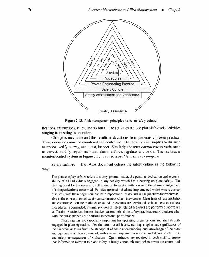
76 Accident Mechanisms and Risk Management _ Chap. 2
Proven Engineering Practice
Safety Culture
Safety Assessment and Verification
Quality Assuran ce
Figure 2.13. Risk management principles basedon safetyculture.
fications, instructions, rules, and so forth. The activities include plant-life-cycle activitiesranging from siting to operation.
Change is inevitable and this results in deviations from previously proven practice.These deviations must be monitored and controlled. The term monitor implies verbs suchas review, verify, survey, audit, test, inspect. Similarly, the term control covers verbs suchas correct, modify, repair, maintain, alarm, enforce, regulate, and so on. The multilayermonitor/control system in Figure 2.13 is called a quality assurance program.
Safety culture. The IAEA document defines the safety culture in the followingway:
The phrasesafety culture refers to a very general matter, the personal dedication and account-ability of all individuals engaged in any activity which has a bearing on plant safety. Thestarting point for the necessary full attention to safety matters is with the senior managementof all organizationsconcerned. Policiesare established and implemented which ensurecorrectpractices, with the recognition that their importance liesnotjust in the practices themselves butalso in theenvironment of safetyconsciousness which theycreate. Clearlinesof responsibilityand communication are established; sound procedures are developed; strictadherence to theseprocedures is demanded; internal reviews of safety related activities are performed; aboveall,staff training andeducation emphasize reasons behind thesafetypractices established, togetherwith the consequences of shortfalls in personal performance.
These matters arc especially important for operating organizations and staff directlyengaged in plant operation. For the latter, at all levels, training emphasizes significance oftheir individual tasks from the standpoint of basic understanding and knowledge of the plantand equipment at their command, with special emphasison reasons underlying safety limitsand safety consequences of violations. Open attitudes arc required in such staff to ensurethat information relevant to plant safety is freelycommunicated; whenerrors are committed,

Sec. 2.3 • Risk Management 77
their admissionis particularlyencouraged. By these means,an all pervadingsafetythinkingisachieved,allowingan inherentlyquestioningattitude,prevention ofcomplacency, commitmentto excellence, and fostering of both personal accountability and corporate self-regulation insafety matters.
Small group activities. Japanese industries make the best use of small-group activitiesto increase productivity and safety. From a safety point of view, such activities stimulate the safetycultureofacompany. Small-groupactivitiesimprovesafetyknowledge bysmall-groupbrainstorming,bottom-upproposal systemsto uncoverhiddencausal relationsand corresponding countermeasures,safety meetingsinvolving people from variousdivisions (R&D, design, production,and marketing),branch factory inspections by heads of other branches, safety exchanges between operation andmaintenance personnel, participation of future operators in the plant constructionand design phase,and voluntary elicitationof near-miss incidents.
The small-groupactivities also boost morale by voluntary presentation of illustrations aboutsafety matters, voluntary tests involving knowledge of plant equipment and procedures, inventingpersonalnicknames for machines,and Shinto purification ceremonies.
The safetyculture is further strengthened by creatingan environment that decreasesrushjobs,and encourages revision, addition, miniaturization, simplification, and systematization of variousprocedures. The culture is supported by management concepts such as 1) rules should be changedif violated,2) learningfrom modelcases rather than accidents,3) permission of small losses,and 4)safety is fundamental for existenceand continuation of the company. •
Proven engineering practices. Devices are designed, manufactured, and con-structed by technologies that are proven by tests and experience, which are reffected inapproved codes and standards and other appropriately documented statements, and that areimplemented by proper selection and training of qualified workers. The use of proven en-gineering methods should continue throughout the plant's life. GMP (good manufacturingpractices) must be vigilantly maintained.
Quality assurance. Quality assurance programs (QA) are a component of modemmanagement. They complement the quality control (QC) programs that normally reside inthe production department. Quality assurance is broader than quality control and has as itsgoal that all items delivered and services and tasks performed meet specified requirements.Organizational arrangements should provide a clear definition of the responsibilities andchannels of communication and coordination for quality assurance. These arrangementsare founded on the principle that the responsibility for achieving quality in a task rests withthose performing it, others verify that the task has been properly performed, and yet othersaudit the entire process. The authority of the quality assurance staff is established firmlyand independently within the organization.
When repairs and modifications are made, analyses are conducted and reviews madeto ensure that the system is returned to a configuration covered in the safety analysis andtechnical specifications. Engineering change orders must be QC and QA monitored. If op-portunities for advancement or improvement over existing practices are available and seemappropriate, changes are applied cautiously only after demonstration that the alternativesmeet the requirements.
Quality assurance practices thus cover validation of designs; supply and use of mate-rials; approval of master device files and manufacturing, inspection, and testing methods;and operational and other procedures to ensure that specifications are met. The associ-ated documents are subject to strict procedures for verification, issue, amendment, andwithdrawal.

78 Accident Mechanisms and Risk Management _ Chap. 2
The relationships between, and the existence of, separate QA, QC, loss prevention,and safety departments vary greatly between industries, large and small companies, andfrequently depend on government regulation. The FDA, the NRC, and the DoD (Departmentof Defense) aJllicense and inspect plants, and each has very detailed and different QA, QC,and safety protocol requirements. Unregulated companies that are not self-insured areusually told what they must do about QA, QC, and safety by their insurance companies'inspectors.
Ethnic and educational diversity; employee lawsuits; massive interference and threatsof closure, fines, and lawsuits by armies of government regulatory agencies (Equal Em-ployment Opportunity Commission, Occupational Safety & Health Administration, En-vironmental Protection Agency, fire inspectors, building inspectors, State Water and AirAgencies, etc.); and adversarial attorneys given the right by the courts to disrupt operationsand interrogate employees have made it difficult for American factory managers to imple-ment, at reasonable cost, anything resembling the Japanese safety and quality programs.Ironically enough, the American company that in 1990 was awarded the prestigious Mal-com Baldridge Award for the best total quality control program in the country declaredbankruptcy in 1991 (see Chapter 12).
Safety assessment and verification. Safety assessments are made before construc-tion and operation of a plant. The assessment should be well documented and independentlyreviewed. It is subsequently updated in the light of significant new safety information.
Safety assessment includes systematic critical reviews of the ways in which struc-tures, systems, and components fail and identifies the consequences of such failures. Theassessment is undertaken expressly to reveal any underlying design weaknesses. The resultsare documented in detail to allow independent audit of scope, depth, and conclusions.
2.3.2 Accident Prevention and Consequence Mitigation
Figure 2.14 shows the phases of accident prevention and accident management. Ac-cident prevention (upper left-hand box) is divided into failure prevention and propagationprevention, while accident management (lower left-hand box) focuses on onsite conse-quence mitigation and offsite consequence mitigation.
In medical terms, failure prevention corresponds to infection prevention, propagationprevention to outbreak prevention, and consequence mitigation to treatment and recoveryafter outbreak.
As shown in the upper right portion of Figure 2.14, neither anticipated disturbancesnor events below the design basis yield accidents if the propagation prevention workssuccessfully. On the other hand, if something is wrong with the propagation preventionor if extreme initiating events are involved, these disturbances or events would develop toevents beyond the design basis, which raises three possibilities: the onsite consequencemitigation works and prevents containment failures and hence offsite releases, the offsiteconsequence mitigation works and minimizes offsite consequences, or all features fail andlarge consequences occur.
2.3.3 Failure Prevention
The first means of preventing failures is to strive for such high quality in design, man-ufacture, construction, and operation of the plant that deviations from normal operations

Sec. 2.3 • Risk Management 79
CQl'C
'8«
CQlEQlCltilc:til~
(/)(/)
(/) '00 '00OJ til tilU eo eoc: c:til c: Cl-e Cl 'iii::J 'iii OJiii OJ 0015
3: "0"0 c:
0 0OJ Q) >0-ro eo OJ0. eo
:~(/)
(/)"E"E OJ "E-c > OJ
W >W
~ ~
-
- - 1-
OffsiteReleases
Risk
Accident
FailurePrevention
ContainmentFailures
Failures andDisturbances
ConsequenceMitigation(Onsite)
ConsequenceMitigation(Offsite)
c:.2CQl>~a..CQl'C
'8«
Consequences
Figure 2.14. Risk-management process.

80 Accident Mechanisms and Risk Management _ Chap. 2
are infrequent and quality products are produced. A deviation may occur from two sources:inanimate device and human. Device-related deviations include ones not only for the plantequipment butalso physical barriers, normalcontrol systems, and emergencysafety systems(see Figure 2.1); some deviations become initiatingevents while others are enabling events.Human-related deviations are further classified into individual, team, and organization.*
2.3.3.1 Device-failure prevention. Device failures are prevented, among otherthings, by proven engineering practice and quality assurance programs. Some examplesfoJlow.
Safety margins. Metal bolts with a larger diameter than predicted by theoreticalcalculation are used. Devices are designed by conservative rules and criteria according tothe proven engineering practice.
Standardization. Functions, materials, and specifications are standardized to de-crease device failure, to facilitatedevice inspection, and to facilitate prediction of remainingdevice lifetime.
Maintenance. A device is periodically inspected and replaced or renewed beforeits failure. This is periodic preventive maintenance. Devices are continuously monitored,and replaced or renewed before failure. This is condition-based maintenance. These typesof monitor-and-control activities are typical elements of the quality assurance program.
Change control. Formal methods of handling engineering and material changesare an important aspect of quality assurance programs. Failures frequently occur due toinsufficient review of system modification. The famous Flixborough accident occurred inEngland in 1974when a pipeline was temporarily installed to bypass one of six reactors thatwas under maintenance. Twenty-eight people died due to an explosion caused by ignitionof flammable material from the defective bypass line.
2.3.3.2 Human-prevention error. Serious accidents often result from incorrecthuman actions. Such events occur when plant personnel do not recognize the safety signif-icance of their actions, when they violate procedures, when they are unaware of conditionsin the plant, when they are misled by incomplete data or incorrect mindset, when they donot fully understand the plant, or when they consciously or unconsciouslycommit sabotage.The operating organizationmustensure that its staff is able to manage the plant satisfactorilyaccording to the risk-management principles iJlustratedin Figure 2.13.
The human-error component of events and accidents has, in the past, been too great.The remedy is a twofold attack: through design, includingautomation, and through optimaluseof human ingenuity when unusualcircumstances occur. This implieseducation. Humanerrors are made by individuals, teams, and organizations.
2.3.3.3 Preventing failures due to individuals. As described in Chapter 10, thehuman is an unbalanced time-sharing system consisting of a slow brain, life-support unitslinked to a large number of sense and motor organs and short- and long-term memoryunits. The human-brainbottleneckresults in phenomenasuch as "shortcut," "perseverance,""task fixation," "alternation," "dependence," "naivety," "queuing and escape," and "grossdiscrimination," which are fully discussed in Chapter 10. Human-machine systems shouldbe designed in such a way that machines help people achieve their potential by giving them
*Human reliability analysis is described in Chapter 10.
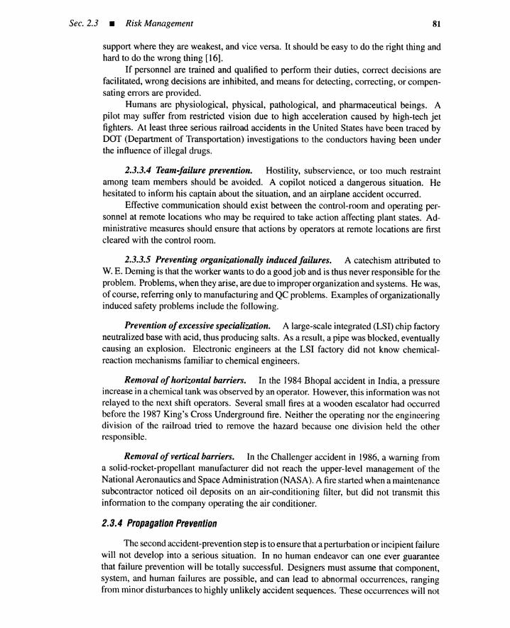
Sec. 2.3 • Risk Management 81
support where they are weakest, and vice versa. It should be easy to do the right thing andhard to do the wrong thing [16].
If personnel are trained and qualified to perform their duties, correct decisions arefacilitated, wrong decisions are inhibited, and means for detecting, correcting, or compen-sating errors are provided.
Humans are physiological, physical, pathological, and pharmaceutical beings. Apilot may suffer from restricted vision due to high acceleration caused by high-tech jetfighters. At least three serious railroad accidents in the United States have been traced byDOT (Department of Transportation) investigations to the conductors having been underthe influence of illegal drugs.
2.3.3.4 Team-failure prevention. Hostility, subservience, or too much restraintamong team members should be avoided. A copilot noticed a dangerous situation. Hehesitated to inform his captain about the situation, and an airplane accident occurred.
Effective communication should exist between the control-room and operating per-sonnel at remote locations who may be required to take action affecting plant states. Ad-ministrative measures should ensure that actions by operators at remote locations are firstcleared with the control room.
2.3.3.5 Preventing organizationally induced failures. A catechism attributed tow. E. Deming is that the worker wants to do a good job and is thus never responsible for theproblem. Problems, when they arise, are due to improper organization and systems. He was,of course, referring only to manufacturing and QC problems. Examples of organizationallyinduced safety problems include the following.
Prevention ofexcessive specialization. A large-scale integrated (LSI) chip factoryneutralized base with acid, thus producing salts. As a result, a pipe was blocked, eventuallycausing an explosion. Electronic engineers at the LSI factory did not know chemical-reaction mechanisms familiar to chemical engineers.
Removal ofhorizontal barriers. In the 1984 Bhopal accident in India, a pressureincrease in a chemical tank was observed by an operator. However, this information was notrelayed to the next shift operators. Several small fires at a wooden escalator had occurredbefore the 1987 King's Cross Underground fire. Neither the operating nor the engineeringdivision of the railroad tried to remove the hazard because one division held the otherresponsible.
Removal of vertical barriers. In the Challenger accident in 1986, a warning froma solid-rocket-propellant manufacturer did not reach the upper-level management of theNational Aeronautics and Space Administration (NASA). A fire started when a maintenancesubcontractor noticed oil deposits on an air-conditioning filter, but did not transmit thisinformation to the company operating the air conditioner.
2.3.4 Propagation Prevention
The second accident-prevention step is to ensure that a perturbation or incipient failurewill not develop into a serious situation. In no human endeavor can one ever guaranteethat failure prevention will be totally successful. Designers must assume that component,system, and human failures are possible, and can lead to abnormal occurrences, rangingfrom minor disturbances to highly unlikely accident sequences. These occurrences will not

82 Accident Mechanisms and Risk Management _ Chap. 2
cause serious consequences if physical barriers, normal control systems, and emergencysafety features remain healthy and operate correctly.
Physical barriers. Physical barriers include safety glasses and helmets, firewalls,trenches, empty space, and-in the extreme case of a nuclear power pIant-concrete bunkersenclosing the entire plant. Every physical barrier must be designed conservatively, its qualitychecked to ensure that margins against failure are retained, and its status monitored.
This barrier itself may be protected by special measures; for instance, a contain-ment structure at a nuclear power plant is equipped with devices that control pressure andtemperature due to accident conditions; such devices include hydrogen ignitors, filteredvent systems, and area spray systems [5]. Safety-system designers ensure to the extentpracticable that the different safety systems protecting physical barriers are functionallyindependent under accident conditions.
Normal control systems. Minor disturbances (usual disturbances and anticipatedabnormal occurrences) for the plant are dealt with through normal feedback control systemsto provide tolerance for failures that might otherwise allow faults or abnormal conditionsto develop into accidents. This reduces the frequency of demand on the emergency safetysystems. These controls protect the physical barriers by keeping the plant in a defined regionof operating parameters where barriers will not be jeopardized. Care in system designprevents runaways that might permit small deviations to precipitate grossly abnormal plantbehavior and cause damage.
Engineeredsafety features andsystems. High reliability in these systems is achievedby appropriate use of fail-safe design, by protection against common-cause failures, by in-dependence between safety systems (inter-independence) and between safety systems andnormal control systems (outer-independence), and by monitor and recovery provisions.Proper design ensures that failure of a single component will not cause loss of function ofthe safety system (a single-failure criterion).
Inter-independence. Complete safety systems can make use of redundancy, di-versity, and physical separations of parallel components, where appropriate, to reduce thelikelihood of loss of vital safety functions. For instance, both diesel-driven and steam-driven generators are installed for emergency power supply if the need is there and moneypermits; different computer algorithms can be used to calculate the same quantity.
The conditions under which equipment is required to perform safety functions maydiffer from those to which it is normally exposed, and its performance may be affected ad-versely by aging or by maintenance conditions. The environmental conditions under whichequipment is required to function are identified as part of a design process. Among theseare conditions expected in a wide range of accidents, including extremes of temperature,pressure, radiation, vibration, humidity, and jet impingement. Effects of external eventssuch as earthquakes should be considered.
Because of the importance of fire as a source of possible simultaneous damage toequipment, design provisions to prevent and combat fires in the plant should be givenspecial attention. Fire-resistant materials are used when possible. Fire-fighting capabilityis included in the design specifications. Lubrication systems use nonflammable lubricantsor are protected against initiation and effects of fires.
Outer-independence. Engineered safety systems should be independent of normalprocess control systems. For instance, the safety shutdown systems for a chemical plant
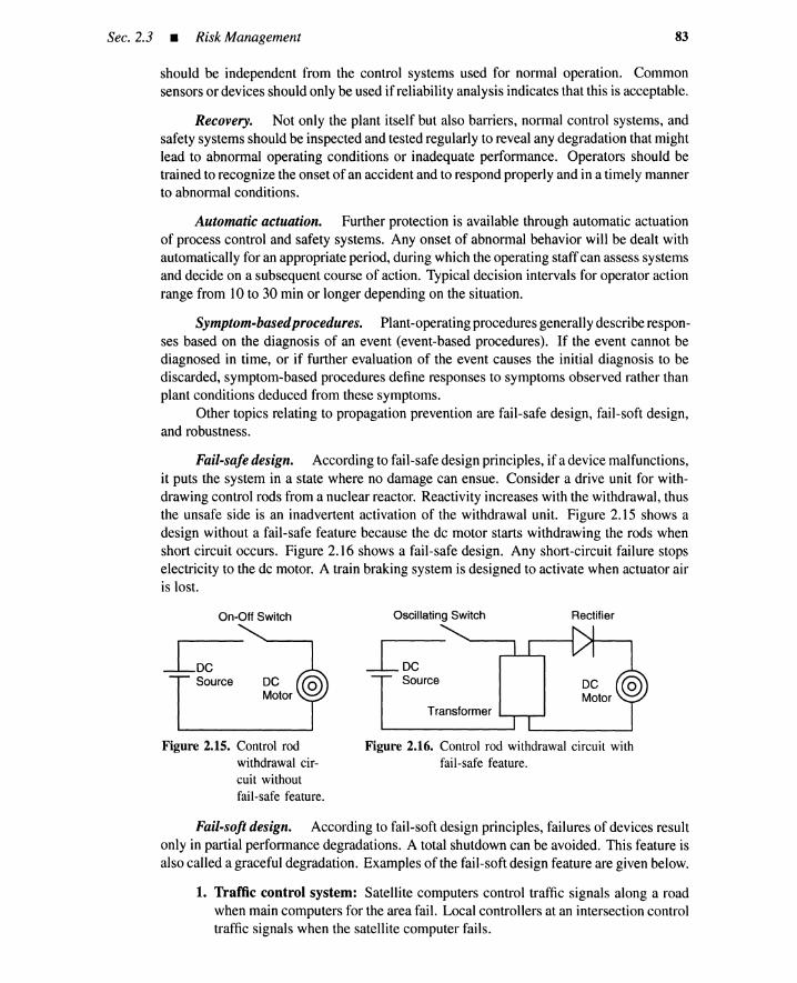
Sec. 2.3 • Risk Management 83
should be independent from the control systems used for normal operation. Commonsensors or devices should only be used if reliability analysis indicates that this is acceptable.
Recovery. Not only the plant itself but also barriers, normal control systems, andsafety systems should be inspected and tested regularly to reveal any degradation that mightlead to abnormal operating conditions or inadequate performance. Operators should betrained to recognize the onset of an accident and to respond properly and in a timely mannerto abnormal conditions.
Automatic actuation. Further protection is available through automatic actuationof process control and safety systems. Any onset of abnormal behavior will be dealt withautomatically for an appropriate period, during which the operating staff can assess systemsand decide on a subsequent course of action. Typical decision intervals for operator actionrange from 10 to 30 min or longer depending on the situation.
Symptom-basedprocedures. Plant-operating procedures generally describe respon-ses based on the diagnosis of an event (event-based procedures). If the event cannot bediagnosed in time, or if further evaluation of the event causes the initial diagnosis to bediscarded, symptom-based procedures define responses to symptoms observed rather thanplant conditions deduced from these symptoms.
Other topics relating to propagation prevention are fail-safe design, fail-soft design,and robustness.
Fail-safe design. According to fail-safe design principles, if a device malfunctions,it puts the system in a state where no damage can ensue. Consider a drive unit for with-drawing control rods from a nuclear reactor. Reactivity increases with the withdrawal, thusthe unsafe side is an inadvertent activation of the withdrawal unit. Figure 2.15 shows adesign without a fail-safe feature because the de motor starts withdrawing the rods whenshort circuit occurs. Figure 2.16 shows a fail-safe design. Any short-circuit failure stopselectricity to the de motor. A train braking system is designed to activate when actuator airis lost.
On-Off Switch Oscillating Switch Rectifier
IDeSource DC
Motor
IDeSource
Transformer ---",---.-.....1
Figure 2.15. Control rodwithdrawal cir-cuit withoutfail-safe feature.
Figure 2.16. Control rod withdrawal circuit withfail-safe feature.
Fail-soft design. According to fail-soft design principles, failures of devices resultonly in partial performance degradations. A total shutdown can be avoided. This feature isalso called a graceful degradation. Examples of the fail-soft design feature are given below.
1. Traffic control system: Satellite computers control traffic signals along a roadwhen main computers for the area fail. Local controllers at an intersection controltraffic signals when the satellite computer fails.

84 Accident Mechanisms and Risk Management _ Chap. 2
2. Restructurable flight-control system: If a rudder plate fails, the remaining rud-ders and thrusts are restructured as a new flight-control system, allowing continu-ation of the flight.
3. Animals: Arteries around open wounds contract and blood flows change, main-taining blood to the brain.
4. Metropolitan water supply: A water supply restriction is enforced during adrought, thus preventing rapid decrease of ground-water levels.
Robustness. A process controller is designed to operate successfully under un-certain environment and unpredictable changes in plant dynamics. Robustness generallymeans the capability to cope with events not anticipated.
2.3.5 Consequence Mitigation
Consequence mitigation covers the period after occurrence of an accident. The oc-currence of an accident means that events beyond a design basis occurred; events below thedesign basis, by definition, could never develop into the accident because normal controlsystems or engineered safety features are assumed to operate as intended.
Because accidents occur, procedural measures must be provided for managing theircourse and mitigating their consequences. These measures are defined on the basis ofoperating experience, safety analysis, and the results of safety research. Attention is givento design, siting, procedures, and training to control progressions and consequences ofaccidents. Limitation of accident consequences are based on safe shutdown, continuedavailability of utilities, adequate confinement integrity, and offsite emergency preparedness.High-consequence, severe accidents are extremely unlikely if they are effectively preventedor mitigated by defense-in-depth philosophy.
As shown in Figure 2.14, consequence mitigation consists of onsite consequencemitigation and offsite consequence mitigation.
Onsite consequence mitigation. This includes preplanned and ad hoc operationalpractices that, in circumstances in which plant design specifications are exceeded, makeoptimum use of existing plant equipment in normal and unusual ways to restore control.This phase would have the objective of restoring the plant to a safe state.
Offsite consequence mitigation. Offsite countermeasures compensate for the re-mote possibility that safety measures at the plant fail. In such a case, effects on the sur-rounding population or the environment can be mitigated by protective actions such assheltering or evacuation of the population. This involves closely coordinated activities withlocal authorities.
Accident management. Onsite and offsite consequence mitigation after occurrenceof an accident is called accident management (Figure 2.14). For severe accidents beyondthe design basis, accident management would come into full play, using normal plantsystems, engineered safety features, special design features, and offsite emergency measuresin mitigation of the effects of events beyond the design basis.
Critique ofaccident management. Events beyond the design basis may, however,develop in unpredictable ways. A Greenpeace International document [10], for instance,evaluates accident management in the following.

Sec. 2.4 • Preproduction Quality Assurance Program 85
The concept of accident managementhas been increasinglystudied and developedinrecent years, and is beginningto be introduced into PRA's. The idea is that even after vitalsafety systems have failed, an accident can still be "managed" by improvising the use ofother systemsfor safetypurposes,and/or by usingsafety systems in a differentcontext thanoriginally planned. The aim is to avoid severe core damage whenever possible; or, failingthat, at least to avoid early containment failure.
Accident management places increased reliance on operator intervention, since ac-cident management strategies must be implemented by plant personnel. The possibilitiesof simulator training, however, are limited. Hence, there is large scope for human errors.This is enhanced by a serious pressure of time in many cases, which will create high psy-chological stress. For this reason alone, the significant reductions in severe core damagefrequency and early containmentfailure probabilitywhichhave been claimed in PRA's (forexample, in the German Risk Study,Phase B) appear completely unrealistic.
Furthermore,accident management,even if performedas planned, might prove inef-fective, leading from one severe accident sequence to another just as hazardous. In somecases, it can even be counter-productive.
Many questions still remain in connection with accident management. In the caseof the German Risk Study, certain accident management measures are considered whichcannotbeperformedinpresent-dayGermanreactors,andrequirecomplicatedandexpensivebackfitting of safety systems.
2.3.6 Summary
Risk management consists of four phases: failure prevention, propagation preven-tion, onsite consequence mitigation, and offsite consequence mitigation. The first two arecalled accident prevention, and the second two accident management. Risk-managementprinciples are embedded in proven engineering practice and quality assurance, built on anurturedsafetyculture. Qualityassuranceconsistsof multilayermonitor/control provisionsthat remove and correct deviations, and safety assessment and verification provisions thatevaluatedeviations.
Failure prevention applies not only to failure of inanimate devices but also humanfailuresby individuals,teams,andorganizations. Onestrivesfor suchhighquality indesign,manufacture, construction,and operationof a plant that deviationsfrom normaloperationalstatesare infrequent. Propagationpreventionensures that a perturbationor incipientfailurewouldnotdevelopintoa moreserioussituationsuchas anaccident. Consequencemitigationcovers the period after occurrence of an accident and includes management of the courseof the accident and mitigating of its consequences.
2.4 PREPRODUCTION QUALITY ASSURANCE PROGRAM
Figure 2.13 showed an overviewof a quality assurance program based on monitor/controlprovisions together with a safety assessment and verification program. This section de-scribes in detail how such programs can be performed for a preproduction design periodthat focuseson the medicalequipment manufacturing industry [6]. In the United StatesandEurope, manufacturers of medical devices are required to have documented PQA (prepro-duction quality assurance) programs and are subject to onsite GMP inspections.
The previous discussions were focused largely on risk reduction from accidents atlarge facilities such as chemical, nuclear, or power plants. From the following, much

86 Accident Mechanisms and Risk Management _ Chap. 2
of the same methodology is seen to apply to reducing the risk of product failures. Muchof this material is adapted from FDAregulatorydocuments [6,11],whichexplains the ukaseprose.
2.4.1 Motivation
Designdeficiency cost. A designdeficiencycan be verycostly once a devicedesignhas been released to production and a device is manufactured and distributed. Costs mayinclude not only replacement and redesign costs, with resulting modifications to manufac-turing procedures and retraining (to enable manufacture of the modifieddevice), but alsoliability costs and loss of customer faith in the market [6].
Device-failure data. Analysis of recall and other adverseexperience data availableto theFDAfromOctober 1983to November 1988indicatesoneof the majorcausesof devicefailures is deficient design; approximately 45% of all recalls were due to preproduction-related problems.
Object. Quality is the composite of all the characteristics, including performance,of an item or product (MIL-STD-l09B). Quality assurance is a planned and systematicpattern of all actions necessary to provide adequate confidence that the device, its compo-nents, packaging, and labeling are acceptable for their intended use (MIL-STD-I09B). Thepurpose of a PQA program is to provide a high degree of confidence that device designsare proven reliable, safe, and effective prior to releasing designs to production for rou-tine manufacturing. No matter how carefully a device may be manufactured, the inherentsafety, effectiveness, and reliability of a device cannot be improvedexcept through designenhancement. It is crucial that adequate controls be established and implemented duringthe design phase to assure that the safety, effectiveness, and reliability of the device areoptimally enhanced prior to manufacturing. An ultimate purpose of the PQA program is toenhance product quality and productivity, while reducing quality costs.
Applicability. The PQA program is applicable to the development of new designsas well as to the adaptation of existing designs to new or improved applications.
2.4.2 Preproduction Design Process
The preproduction design process proceeds in the following sequence: I) establish-ment of specifications, 2) concept design, 3) detail design, 4) prototype production, 5) pilotproduction, and 6) certification (Figure 2.17). This process is followed by a postdesignprocess consisting of routine production, distribution, and use.
Specification. Design specifications are a description of physical and functionalrequirements for an article. In its initial form, the design specification is a statementof general functional requirements. The design specification evolves through the R&Dphase to reflect progressive refinements in performance, design, configuration, and testrequirements.
Prior to the actual design activity,the design specifications should be defined in termsof desired characteristics, such as physical, chemical, and performance. The performancecharacteristics include safety, durability/reliability, precision, stability, and purity. Ac-ceptable ranges or limits should be provided for each characteristic to establish allowablevariationsand these should be expressed in terms that are readily measurable. For example,the pulse-amplitude range for an external pacemaker could be established as 0.5 to 28mAat an electrical load of 1000ohms, and pulse duration could be 0.1 to 9.9ms.

Sec. 2.4 • Preproduction Quality Assurance Program
Preproduction Design PostdesignProcess Process
1 1Specifications [
Prototype[
RoutineProduction Production
t + t
Concept Pilot I DistributionDesign Product ion
t t t
Detail Certification UseDesign
l I
Figure 2.17. Preproduction design processfollowed by postdesign process.
87
The desig n aim should be translated into written design specifications. The expecteduse of the device, the user, and user environme nt should be considered.
Concept and detail design. The actual device evolves from concep t to detail de-sign to satisfy the specifications. In the deta il design, for instance, suppliers of parts andmateria ls (PIM ) used in the device; software clements developed in-house; custom softwarefrom contractors; manuals, charts, inserts, panels, display labels; packaging; and supportdocumentation such as test specifica tions and instruct ions are deter mined.
Prototype production. Prototypes are developed in the laboratory or machine shop.During this production, conditions are typically better controlled and personnel more knowl-edgeable about what needs to be done and how to do it than production personnel. Thusthe prototype production differs in conditions from pilot and routine productions.
Pilot production. Before the specifications are released for routine production,actual-finished devices should be manufactured using the approved specifications, the samematerials and components, the same or similar production and quality control equipment ,and the methods and procedures that will be used for routine production. This type ofproduction is essential for assuring that the routine manufacturing process will producethe intended devices without adverse ly affect ing the devices . The pilot production is anecessary part of process validation [II].
2.4.3 Design Review for paA
The design review is a planned, scheduled, and documented audit of all pertinentaspects of the design that can affect safety and effectiveness. Such a review is a kernel of thePQA program. Each manufacturer should estab lish and implement an independent reviewof the design at each stage as the design matures. The design review assures conformanceto design criteria and identifies design weaknesses. The objective of design review is theearly detection and remedy of des ign deficiencies. The earlier design review is initiated,the sooner problems can be identified and the less cost ly it will be to implement correctiveaction.

88 Accident Mechanisms and Risk Management _ Chap. 2
Checklist. A design review checklist could include the following.
1. Physical characteristics and constraints
2. Regulatory and voluntary standards requirements
3. Safety needs for the user, need for fail-safe characteristics
4. Producibility of the design
5. Functional and environmental requirements
6. Inspectability and testability of the design, test requirements
7. Permissible maximum and minimum tolerances
8. Acceptance criteria
9. Selection of components
10. Packaging requirements
11. Labeling, including warnings, identification,operation, and maintenance instruc-tions
12. Shelf-life, storage, stability requirements
13. Possible misuse of the product that can be anticipated, elimination of human-induced failures
14. Product serviceability/maintainability
Specification changes. Changes made to the specificationsduring R&D should bedocumented and evaluated to assure that they accomplish the intended result and do notcompromise safety or effectiveness. Manufacturers should not make unqualified, undoc-umented changes during preproduction trials in response to suggestions or criticism fromusers. In the manufacturer's haste to satisfy the user, changes made without an evaluationof the overall effect on the device could result in improving one characteristic of the devicewhile having an unforeseen adverse effect on another.
Concept and detail design. A device's compatibility with other devices in theintended operating system should be addressed in the design phase, to the extent that com-patibility is necessary to assure proper functioning of the system. The full operating rangeof within-tolerancespecificationsfor the mating device(s) should be considered, not merelynominal values.
A disposable blood tubing set was designed and manufactured by Company A foruse with Company B's dialysis machine. The tubing was too rigid, such that when theair-embolism occlusion safety system on the dialysis machine was at its lowest within-specification force, the tubing would not necessarily occlude and air could be passed to thepatient. The tubing occluded fully under the nominal occlusion force.
Quick fixes should be prohibited. These include adjustments that may allow thedevice to perform adequately for the moment, but do not address the underlying cause.All design defects should be corrected in a manner that will assure the problem will notrecur.
Identification ofdesign weakness. Potential design weakness should be identifiedby FMECA (failure mode effects criticality analysis) or PTA(fault-tree analysis). FMECAis described in MIL-STD-1629A [12].*
*See Chapter 3 of this book for FMEA and FMECA. See Chapter 4 for FTA.

Sec. 2.4 • Preproduction QualityAssurance Program 89
FMEA (failure mode and effects analysis) is a process of identifying potential designweaknesses through reviewing schematics, engineering drawings, and so on, to identifybasic faults at the partJmateriallevel and determine their effect at finished or subassemblylevel on safety and effectiveness. PTA is especially applicable to medical devices becausehuman/device interfaces can be taken into consideration, that is, a particular kind of adverseeffect on a user, such as electrical shock, can be assumed as a top event to be analyzed. Thedesign weakness is expressed in terms of a failure mode, that is, a manner or a combinationof basic human/component failures in which a device failure is observed.
FMEA, FMECA, or PTA should include an evaluation of possible human-inducedfailures or hazardous situations. For example, battery packs were recalled because of aninstance when the battery pack burst while being charged. The batteries were designed tobe trickle charged, but the user charged the batteries using a rapid charge. The result was arapid build-up of gas that could not be contained by the unvented batteries.
For those potential failure modes that cannot be corrected through redesign effort,special controls such as warning labels, alarms, and so forth, should be provided. Forexample, if a warning label had been provided for the burst batteries pack, or the batteriesvented, the incident probably would not have happened. As another example, one possiblefailure mode for an anesthesia machine could be a sticking valve. If the valve's stickingcould result in over- or underdelivery of the desired anesthesia gas, a fail-safe feature shouldbe incorporated into the design to prevent the wrong delivery, or if this is impractical, asuitable alarm system should be included to alert the user in time to take corrective action.
When a design weakness is identified, consideration should be made of other dis-tributed devices in which the design weakness may also exist. For example, an anomalythat could result in an incorrect output was discovered in a microprocessor used in a blood-analysis diagnostic device at a prototype-testing stage. This same microprocessor was usedin other diagnostic machines already in commercial distribution. A review should havebeen made of the application of the microprocessor in the already-distributed devices toassure that the anomaly would not adversely affect performance.
Reliability assessment. Prior to commercial distribution, reliability assessment maybe initiated by theoretical and statistical methods by first determining the reliability of eachcomponent, then progressing upward, establishing the reliability of each subassembly andassembly, until the reliability of the entire device or device system is established. References[13] and [14] apply to predicting the reliability of electronic devices. Component reliabilitydata sources are well reviewed in [15].*
This type of reliability assessment does not simulate the actual effect of interactionof system parts and the environment. To properly estimate reliability, complete devices anddevice systems should be tested under simulated-use conditions.
Parts and materials quality assurance. Parts and materials should be selectedon the basis of their suitability for the chosen application, compatibility with other PIMand the environment, and proven reliability. Conservative choices in selection of PIM arecharacteristic of reliable devices. Standard proven PIMshould be used as much as possiblein lieu of unproven P/M.
For example, a manufacturer used an unproven plastic raw material in the initialproduction of molded connectors. After distribution, reports were received that the tubing
*See Chapters 6 and 7 for quantification of component reliability. Chapters 8 and 9 describe quantificationof system reliability parameters.
90 Accident Mechanisms and Risk Management • Chap. 2
was separating from the connectors. Investigation and analysis by the manufacturer revealedthat the unproven plastic material used to mold the connectors deteriorated with time,causing a loss of bond strength. The devices were subsequently recalled.
The PIM quality assurance means not only assuring PIM will perform their functionsunder normal conditions but that they are not unduly stressed mechanically, electrically,environmentally, and so on. Adequate margins of safety should be established when nec-essary. A whole-body image device was recalled because screws used to hold the upperdetector head sheared off, allowing the detector head to fall to its lowest position. Thescrews were well within their tolerances for all specified attributes under normal condi-tions. However, the application was such that the screws did not possess sufficient shearstrength for the intended use.
When selecting PIM previously qualified, attention should be given to the currentnessof the data, applicability of the previous qualification to the intended application, andadequacy of the existing P/M specification. Lubricant seals previously qualified for use inan anesthesia gas circuit containing one anesthesia gas may not be compatible with anothergas. These components should be qualified for each specific environment.
Failure of PIM during qualification should be investigated and the result described inwritten reports. Failure analysis, when deemed appropriate, should be conducted to a levelsuch that the failure mechanism can be identified.
Software quality assurance. Software quality assurance (SQA) should begin witha plan, which can be written using a guide such as ANSI/IEEE Standard 730-1984, IEEEStandard for Software Quality Assurance Plans. Good SQA assures quality software fromthe beginning of the development cycle by specifying up front the required quality at-tributes of the completed software and the acceptance testing to be performed. In addition,the software should be written in conformance with a company standard using structuredprogramming. When device manufacturers purchase custom software from contractors, theSQA should assure that the contractors have an adequate SQA program.
Labeling. Labeling includes manuals, charts, inserts, panels, display labels, testand calibration protocols, and software for CRT display. A review of labeling should assurethat it is in compliance with applicable laws and regulations and that adequate directionsfor the product's intended use are easily understood by the end-user group. Instructionscontained in the labeling should be verified.
After commercial distribution, labeling had to be corrected for a pump because therewas danger of overflow if certain flow charts were used. The problem existed because anerror was introduced in the charts when the calculated flow rates were transposed onto flowcharts.
Manufacturers of devices that are likely to be used in a home environment and oper-ated by persons with a minimum of training and experience should design and label theirproducts to encourage proper use and to minimize the frequency of misuse. For example,an exhalation valve used with a ventilator could be connected in reverse position becausethe inlet and exhalation ports were the same diameter. In the reverse position the user couldbreathe spontaneously but was isolated from the ventilator. The valve should have beendesigned so that it could be connected only in the proper position.
Labeling intended to be permanently attached to the device should remain attachedand legible through processing, storage, and handling for the useful life of the device.Maintenance manuals should be provided where applicable and should provide adequateinstructions whereby a user or service activity can maintain the device in a safe and effectivecondition.

Sec. 2.4 • Preproduction QualityAssurance Program 91
Simulatedtestingfor prototype production. Use testing should not begin until thesafety of the device from the prototype production has been verified under simulated-useconditions, particularly at the expected performance limits. Simulated-use testing shouldaddress use with other applicabledevices and possiblemisuse. Devices in a home environ-ment should typically anticipate the types of operator errors most likely to occur.
Extensivetestingfor pilotproduction. Devices from the pilot production shouldbe qualified through extensive testing under actual- or simulated-useconditions and in theenvironment, or simulatedenvironment, in which the device is expected to be used.
Proper qualification of devices that are produced using the same or similar methodsand procedures as those to be used in routine production can prevent the distribution andsubsequent recall of many unacceptable products. A drainage catheter using a new ma-terial was designed, fabricated, and subsequently qualified in a laboratory setting. Oncethe catheter was manufactured and distributed, however, the manufacturer began receiv-ing complaints that the bifurcated sleeve was separating from the catheter shrink base.Investigation found the separation was due to dimensional shrinkage of the material andleeching of the plasticizers from the sleeve due to exposure to cleaning solutions duringmanufacturing. Had the device been exposed to actual production conditions during fab-rication of the prototypes, the problem may have been detected before routine productionand distribution.
When practical, testing should be conducted using devices produced from the pilotproduction. Otherwise, the qualified device will not be truly representative of productiondevices. Testingshould include stressing the device at its performance and environmentalspecification limits.
Storage conditions should be considered when establishingenvironmental test spec-ifications. For example, a surgical staple device was recalled because it malfunctioned.Investigation found that the device malfunctionedbecause of shrinkage of the plastic cut-ting ring due to subzero conditions to which the device was exposed during shipping andstorage.
Certification. Thecertificationisdefinedasadocumentedreviewofallqualificationdocumentation prior to releaseof thedesignfor production. Thequalification here isdefinedas a documented determination that a device (and its associated software), component,packaging, or labeling meet all prescribed design and performance requirements. Thecertification should include a determinationof the
1. resolutionof anydifferencebetweenthe proceduresand standardsusedto producethe design while in R&D and those approvedfor production
2. resolution of any differences between the approved device specifications and theactual manufacturedproduct
3. validity of test methods used to determine compliance with the approved specifi-cations
4. adequacy of specifications and specification change control program
5. adequacy of the complete quality assurance plan
Postproduction quality monitoring. The effort to ensure that the device and itscomponents have acceptable quality and are safe and effective must be continued in themanufacturing and use phase, once the design has been proven safe and effective anddevices are produced and distributed.

92 Accident Mechanisms and Risk Management • Chap. 2
2.4.4 Management and Organizational Matters
Authorities and responsibilities. A PQA program should be sanctioned by uppermanagement and should be considered a crucial part of each manufacturer's overall effortto produce only reliable, safe, and effective products. The organizational elements andauthorities necessary to establish the PQA program, to execute program requirements, andto achieve program goals, should be specified in formal documentation. Responsibilityfor implementing the overall program and each program element should also be formallyassignedand documented. The SQA representativeor department should have the authorityto enforce implementationof SQA policies and recommendations.
Implementation. The design reviewprogram should be established as a permanentpart of the PQA and the design review should be conducted periodically throughout thepreproductionlife-cyclephaseas thedesign maturestoassureconformancetodesigncriteriaand to identify design weaknesses. The PQA program including the design review shouldbe updated as experience is gained and the need for improvement is noted.
Design reviewsshould, whenappropriate, includeFMECAandFTAto identifypoten-tial design weaknesses. When appropriate and applicable, the reliabilityassessment shouldbe made for new and modifieddesigns and acceptable failure rates should be established.The review of labeling should be included as part of the design review process.
Each manufacturermusthavean effectiveprogramfor identification of failurepatternsor trends and analysis of quality problems, taking appropriate corrective actions to preventrecurrenceof theseproblems,and the timely internalreportingof problemsdiscoveredeitherin-houseor in the field. Specificinstructionsshouldbeestablishedto providedirectionaboutwhen and how problems are to be investigated, analyzed, and corrected, and to provideresponsibility for assuring initiation and completion of these tasks.
Procedures. Device design should progress through clearly defined and plannedstages, starting with the concept design and ending in the pilot production. A detailed,documented description of the design-review program should be established, includingorganizational units involved, procedures used, flow diagrams of the process, identificationof documentation required, a schedule, and a checklist of variables to be considered andevaluated. The SQA program should include a protocol for formal review and validationof device software to ensure overall functional reliability.
Testing should be performed according to a documented test plan that specifies theperformance parameters to be measured, test sequence, evaluation criteria, test environ-ment, and so on. Once the device is qualified, all manufacturing and quality assurancespecificationsshould be placed under formal change control.
Staffing. Reviews should be objective, unbiased examinations by appropriatelytrained, qualified personnel, which should include individualsother than those responsiblefor the design. For example, design review should be conducted by representatives ofManufacturing,Quality Assurance, Engineering, Marketing, Servicing, and Purchasing, aswell as those responsible for R&D.
Change control. When corrective action is required, the action should be appro-priately monitored, with responsibilityassigned to assure that a follow-up is properly con-ducted. Schedules should be established for completing corrective action. Quick fixesshould be prohibited.
Chap. 2 • References 93
When problem investigation and analysis indicate a potential problem in the design,appropriate design improvements must be made to prevent recurrence of the problem. Anydesign changes must undergo sufficient testing and preproduction evaluation to assure thatthe revised design is safe and effective. This testing should include testing under actual- orsimulated-use conditions and clinical testing as appropriate to the change.
Documentation and communication. Review results should be well documentedin report form and signed by designated individuals as complete and accurate. All changesmade as a result of review findings should be documented. Reports should include con-clusions and recommended follow-up and should be disseminated in a timely manner toappropriate organizational elements, including management.
Failure reports of PIM should be provided to management and other appropriatepersonnel in a timely manner to assure that only qualified PIMare used.
A special effort should be made to assure that failure data obtained from complaintand service records that may relate to design problems are made available and reviewed bythose responsible for design.
2.4.5 Summary
A preproduction quality assurance program is described to illustrate quality assurancefeatures based on monitor/control loops and safety assessment and verification activities.The program covers a preproduction design process consisting of design specifications,concept design, detail design, prototype production, pilot production, and certification. ThePQA program contains design review, which deals with checklist, specification, concept anddetail design, identification ofdesign weaknesses, reliability assessment, parts and materialsquality assurance, software quality assurance, labeling, prototype production testing, pilotproduction testing, and so forth. The PQA ensures smooth and satisfactory design transferto a routine production. Management and organizational matters are presented from thepoints of view ofauthorities and responsibilities, PQA program implementation, procedures,staffing requirements, documentation and communication, and change control.
REFERENCES
[1] Reason, J. Human Error. New York: Cambridge University Press, 1990.
[2] Wagenaar, W. A., P. T. Hudson, and J. T. Reason. "Cognitive failures and accidents."Applied Cognitive Psychology, vol. 4, pp. 273-294, 1990.
[3] Embrey, D. E. "Incorporating management and organizational factors into prob-abilistic safety assessment." Reliability Engineering and System Safety, vol. 38,pp. 199-208, 1992.
[4] Lambert, H. E. "Case study on the use of PSA methods: Determining safety impor-tance of systems and components at nuclear power plants." IAEA, IAEA- TECDOC-590,1991.
[5] International Nuclear Safety Advisory Group. "Basic safety principles for nuclearpower plants." IAEA, Safety series, No. 75-INSAG-3, 1988.
[6] FDA. "Preproduction quality assurance planning: Recommendations for medical de-vice manufacturers." The Food and Drug Administration, Center for Devices andRadiological Health, Rockville, MD, September 1989.
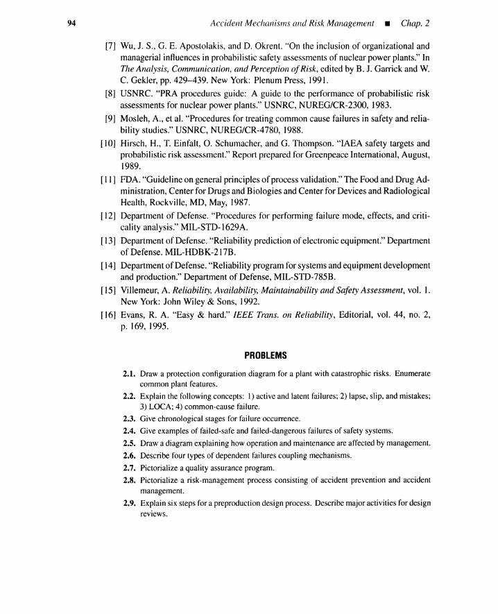
94 Accident Mechanisms and Risk Management _ Chap. 2
[7] Wu, J. S., G. E. Apostolakis, and D. Okrent. "On the inclusion of organizational andmanagerial influences in probabilistic safety assessments of nuclear power plants." InThe Analysis, Communication, and Perception ofRisk, edited by B. J. Garrick and W.C. Gekler, pp. 429-439. New York: Plenum Press, 1991.
[8] USNRC. "PRA procedures guide: A guide to the performance of probabilistic riskassessments for nuclear power plants." USNRC, NUREG/CR-2300, 1983.
[9] Mosleh, A., et al. "Procedures for treating common cause failures in safety and relia-bility studies." USNRC, NUREG/CR-4780, 1988.
[10] Hirsch, H., T. Einfalt, O. Schumacher, and G. Thompson. "IAEA safety targets andprobabilistic risk assessment." Report prepared for Greenpeace International, August,1989.
[ II] FDA. "Guideline on general principles of process validation." The Food and Drug Ad-ministration, Center for Drugs and Biologies and Center for Devices and RadiologicalHealth, Rockville, MD, May, 1987.
[12] Department of Defense. "Procedures for performing failure mode, effects, and criti-cality analysis." MIL-STD-1629A.
[13] Department of Defense. "Reliability prediction of electronic equipment." Departmentof Defense. MIL-HDBK-217B.
[14] Department of Defense. "Reliability program for systems and equipment developmentand production." Department of Defense, MIL-STD-785B.
[15] Villemeur, A. Reliability, Availability, Maintainability and Safety Assessment, vol. I.New York: John Wiley & Sons, 1992.
[16] Evans, R. A. "Easy & hard." IEEE Trans. on Reliability, Editorial, vol. 44, no. 2,p. 169, 1995.
PROBLEMS
2.1. Draw a protection configuration diagram for a plant with catastrophic risks. Enumeratecommonplant features.
2.2. Explainthe following concepts: I) activeand latent failures; 2) lapse, slip, and mistakes;3) LOCA;4) common-cause failure.
2.3. Givechronological stages for failureoccurrence.
2.4. Giveexamplesof failed-safe and failed-dangerous failuresof safety systems.
2.5. Drawa diagramexplaininghowoperationand maintenance are affectedby management.
2.6. Describefour types of dependent failures coupling mechanisms.
2.7. Pictorialize a quality assuranceprogram.
2.8. Pictorialize a risk-management process consisting of accident prevention and accidentmanagement.
2.9. Explainsix steps for a preproduction designprocess. Describemajoractivitiesfor designreviews.

robabilistic RiskAssessment
3.1 INTRODUCTION TO PROBABILISTIC RISK ASSESSMENT
3.1.1 Initiating-Event and Risk Profiles
Initiatingevents. From a risk-analysis standpoint there can be no bad ending if thereis a good beginning. There are, regrettably, a variety of bad beginnings. In probabilisticrisk assessment, bad beginnings are called initiating events or accident initiators. Withoutinitiating events, no accident can occur. PRA is a methodology that transforms initiatingevents into risk profiles.
A plant with four risk-mitigation features was shown in Figure 2.1. They are physicalbarriers, normal control systems, emergency safety systems, and onsite and offsite emer-gency countermeasures. Initiating events are denoted as a "challenge." Risk profiles for theplant result from correlating the damage done with the frequency of accident occurrence.
Onsite and offsite consequences can be prevented or mitigated by a risk-managementprocess consisting of the four phases shown in Figure 2.14. An initiating event is a fail-ure. Thus the four phases are initiating-event prevention, initiating-event-propagation pre-vention, onsite consequence mitigation, and offsite consequence mitigation. Occurrencelikelihoods of initiating events are decreased by prevention actions. An initiating event,once it occurs, is subject to initiating-event-propagation prevention. If an initiating eventdevelops into an accident, then onsite and offsite consequence mitigations to halt accidentprogression and to mitigate consequences take place.
For consequences to occur, an initiating event must occur; this event must progressto an accident, and this accident must progress sufficiently to yield onsite and offsite con-sequences. This chain is similar to an influenza outbreak. Contact with the virus is aninitiating event; an outbreak of flu is an accident; patient death is an onsite consequence;airborne infections have offsite consequences. Initiating events are transformed into riskprofiles that depend on the relevant risk-management process. PRA provides a systematicapproach for clarifying the transformation of an initiating event into a risk profile.
95

96 Probabilistic Risk Assessment _ Chap. 3
It should be noted that risk profilesare not the only products of a risk study. The PRAprocessanddata identify vulnerabilitiesinplantdesignand operation. PRApredictsgeneralaccident scenarios, although some specificdetails might be missed. No other approach hassuperior predictiveabilities [1].
3.1.2 Plants without Hazardous Materials
PRA is not restricted to a plant containing hazardous materials; PRA applies to allengineered systems or plants, with or without material hazards. The PRA approach issimpler for plants without hazardous materials. Additional steps are required for plantswith material hazards because material releases into the environment must be analyzed.Using the medical analogy, both infectious and noninfectious diseases can be dealt with.
Passenger railway. As an example of a system without material hazards, considera single track passenger railway consisting of terminals A and B and a spur between theterminals (Figure 3.1). An unscheduled departure from terminal A that follows failure toobserve red departure signal 1 is an initiating event. This type of departure occurred inJapan when the departure signal was stuck red because of a priority override from terminalB. This override was not communicated to terminal A personnel, who assumed that thered signal was not functioning. The traffic was heavy and the terminal A train conductorneglected the red signal and started the train.
A 1°1-1
Red
c
LSpur ~~ Green
FP~Green
Figure 3.1. A single track railway with departure-monitoringdevice.
The railway has a departure-monitoringdevice (DM), designed to prevent accidentsdue to unscheduleddepartures by changing trafficsignal 3 at the spur entrance to red, thuspreventing a terminal B train from entering region C between the spur and terminal A.However, this monitoring device was not functioning because it was under maintenancewhen the departure occurred. A train collision occurred in region C, and 42 people died.
The unscheduled departure as an initiating event would not have yielded a traincollision in region C if the departure monitoring device had functioned, and the terminal Btrain had remained on the main track between B and the spur until the terminal A train hadentered the spur.
Twocases are possible-collision and no collision. Suppose that the terminal B trainhas not passed the spur signal whenthe terminalA traincommits the unscheduleddeparture:this defines a particular type of initiating event. Another type of initiating event would bean unscheduled departure after the terminal B train crosses the spur signal. Suppose alsothat the railway has many curves and that a collision occurs whenever there are two trainsmoving in opposite directions in region C.
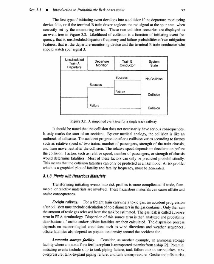
Sec. 3.1 • Introduction to Probabilistic Risk Assessment 97
The first type of initiating event develops into a collision if the departure-monitoringdevice fails, or if the terminal B train driver neglects the red signal at the spur area, whencorrectly set by the monitoring device. These two collision scenarios are displayed asan event tree in Figure 3.2. Likelihood of collision is a function of initiating-event fre-quency, that is, unscheduled departure frequency, and failure probabilities of two mitigationfeatures, that is, the departure-monitoring device and the terminal B train conductor whoshould watch spur signal 3.
Unscheduled Departure Train B SystemTrain A
DepartureMonitior Conductor State
Success No Collision
Success
FailureCollision
FailureCollision
Figure 3.2. A simplified event tree for a single track railway.
It should be noted that the collision does not necessarily have serious consequences.It only marks the start of an accident. By our medical analogy, the collision is like anoutbreak of a disease. The accident progression after a collision varies according to factorssuch as relative speed of two trains, number of passengers, strength of the train chassis,and train movement after the collision. The relative speed depends on deceleration beforethe collision. Factors such as relative speed, number of passengers, or strength of chassiswould determine fatalities. Most of these factors can only be predicted probabilistically.This means that the collision fatalities can only be predicted as a likelihood. A risk profile,which is a graphical plot of fatality and fatality frequency, must be generated.
3.1.3 Plants with Hazardous Materials
Transforming initiating events into risk profiles is more complicated if toxic, flam-mable, or reactive materials are involved. These hazardous materials can cause offsite andonsite consequences.
Freight railway. For a freight train carrying a toxic gas, an accident progressionafter collision must include calculation ofhole diameters in the gas container. Only then canthe amount of toxic gas released from the tank be estimated. The gas leak is called a sourceterm in PRA terminology. Dispersion of this source term is then analyzed and probabilitydistributions of onsite and/or offsite fatalities are then calculated. The dispersion processdepends on meteorological conditions such as wind directions and weather sequences;offsite fatalities also depend on population density around the accident site.
Ammonia storage facility. Consider, as another example, an ammonia storagefacility where ammonia for a fertilizer plant is transported to tanks from a ship [2]. Potentialinitiating events include ship-to-tank piping failure, tank failure due to earthquakes, tankoverpressure, tank-to-plant piping failure, and tank underpressure. Onsite and offsite risk

98 Probabilistic Risk Assessment _ Chap. 3
profilescan becalculatedby a proceduresimilar to theone usedfor the railwaytraincarryingtoxic materials.
Oil tanker. For an oil tanker, an initiating event could be a failure of the marineengine system. This can lead to a sequence of events, that is, drifting, grounding, oilleakage, and sea pollution. A risk profile for the pollution or oil leakage can be predictedfrom informationabout frequency of engine failure as an accident initiator; initiating-eventpropagation to the start of the accident, that is, the grounding; accident-progression analysisafter grounding; source-term analysis to determine the amount of oil released; released oildispersion; and degree of sea pollution as an offsite consequence.
3.1.4 Nuclear Power Plant PRA: WASH-1400
LOCA event tree. Consideras an example the reactorsafetystudy,WASH-1400, anextensive risk assessment of nuclear power plants sponsored by the United States AtomicEnergy Commission (AEC) that was completed in 1974. This study includes the sevenbasic tasks shown in Figure 3.3 [3]. It was determined that the overriding risk of a nuclearpower plant was that of a radioactive (toxic) fission product release, and that the criticalportion of the plant, that is, the subsystem whose failure initiates the risk, was the reactorcooling system. The PRA begins by following the potential course of events beginningwith (coolant) "pipe breaks," this initiating event having a probability or a frequency of PA
in Figure 3.4. This initiating event is called a loss of coolant accident. The second phasebegins, as shown in Figure 3.3, with the task of identifying the accident sequences: thedifferent ways in which a fission product release might occur.
1 3 4 5 6
Identification Fission Distribution Health Overallof Accident Product of Source Effects RiskSequences ~ Released --. in the --+- and ~ Assessment
from Environment PropertyContainment Damage
t t2 7
Assignment Analysisof of Other
Probability RisksValues
Figure 3.3. Sevenbasic tasks in a reactor safety study.
Fault-tree analysis. PTA was developed by H. A. Watson of the Bell TelephoneLaboratories in 1961 to 1962during an Air Force study contract for the MinutemanLaunchControl System. The first published papers were presented at the 1965 Safety Sympo-sium sponsored by the Universityof Washington and the Boeing Company, where a groupincluding D. F. Haasl, R. J. Schroder, W. R. Jackson, and others had been applying andextending the technique. Fault trees (FTs) were used with event trees (ETs) in the WASH-1400study.
Since the early 1970s when computer-basedanalysis techniques for FTs were devel-oped, their use has become very widespread.* Indeed, the use of PTA is now mandated bya number of governmental agencies responsible for worker and/or public safety. Risk-as-
*Computercodes are listed and described in reference [4].
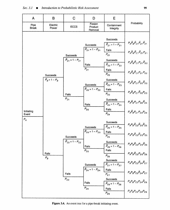
Sec. 3.1 • Introduction to Probabilistic Risk Assessment 99
A B C D E
Pipe Electric Fission ContainmentProbability
ECCS ProductBreak PowerRemoval
Integrity
Succeeds
Succeeds PE1=1 - PE1PAP8Pc 1Po1PE1
Po1=1 - Po1 Fails - - -PE1
PAPBPC1Po1PE1Succeeds
PC1=1 - PC1 SucceedsPAPBPC1Po1PE2
Fails PE2 =1 - PE2Po1 Fails
PAPBPc 1Po1PE2Succeeds PE2
PB= 1 - PB SucceedsPAPBPC1Po2PE3
Succeeds PE3 =1 - PE3
Po2 =1 - Po2 FailsPAPBPC1Po2PE3
Fails PE3
PC1 SucceedsPAP8PC1Po2PE4
Fails PE4 =1 - PE4
InitiatingPo2 Fails
PAP8PC1Po2PE4Event PE4
PASucceeds - - -
Succeeds PE5 =1 - PE5PAPBPC2Po3PE5
P03 =1 - P03 Fails - -Succeeds PE5
PAPBPC2Po3PE5
PC2 =1 - PC2 SucceedsPAPBPC2P03PE6
Fails PE6 =1 - PE6Po3 Fails
FailsPE6
PAPBPc 2Po3PE6
P8Succeeds
PAP8PC2Po4PE7Succeeds PE7 =1 - PE7
Po4 =1 - P04 FailsPAP8PC2P04PE7Fails PE7
PC2 Succeeds
Fails PE8 =1 - PE8PAPBPC2P04PE8
P04 Fails
PE8PAPBPC2P04PE8
Figure 3.4. An event tree for a pipe-breakinitiatingevent.

100 Probabilistic Risk Assessment _ Chap. 3
sessment methodologiesbasedon FTs and ETs (called a level I PRA) are widely used in var-ious industries including nuclear, aerospace, chemical, transportation, and manufacturing.
The WASH-1400study used fault-tree techniques to obtain, by backward logic, nu-merical values for the P's in Figure 3.4. This methodology, which is described in Chapter 4,seeks out the equipment or human failures that result in top events such as the pipe breakor electric power failure depicted in the headings in Figure 3.4. Failure rates, based on datafor component failures, operator error, and testing and maintenance error are combinedappropriately by means of fault-tree quantification to determine the unavailability of thesafety systems or an annual frequency of each initiating event and safety system failure.This procedure is identified as task 2 in Figure 3.3.
Accident sequence. Now let us return to box I of Figure 3.3, by considering theevent tree (Figure 3.4) for a LOCA initiating event in a typical nuclear power plant. Theaccident starts with a coolant pipe break having a probability (or frequency) of occurrencePA. The potential course of events that might follow such a pipe break are then examined.Figure 3.4 is the event tree, which shows all possible alternatives. At the first branch, thestatus of the electric power is considered. If it is available, the next-in-line system, theemergency core-cooling system, is studied. Failure of the ECCS results in fuel meltdownand varying amounts of fission product release, depending on the containment integrity.
Forward versus backward logic. It is important to recognize that event trees areused to defineaccident sequences that involvecomplex interrelationshipsamong engineeredsafety systems. They are constructed using forward logic: We ask the question "Whathappens if the pipe breaks?" Fault trees are developed by asking questions such as "Howcould the electric power fail?" Forward logic used in event-tree analysis and FMEA isoften referred to as inductive logic, whereas the type of logic used in fault-tree analysis isdeductive.
Event-tree pruning. In a binary analysis of a system that either succeeds or fails, thenumber of potential accident sequences is 2N , where N is the number of systemsconsidered.In practice, as will be shown in the followingdiscussion, the tree of Figure 3.4can bepruned,by engineering logic, to the reduced tree shown in Figure 3.5.
One of the first things of interest is the availability of electric power. The question is,what is the probability, PB, of electric power failing, and how would it affect other safetysystems? If there is no electric power, the emergency core-cooling pumps and sprays areuseless-in fact, none of the postaccident functions can be performed, Thus, no choicesare shown in the simplified event tree when electric power is unavailable and a very largerelease with probability PAX PB occurs. In the event that the unavailabilityof electric powerdepends on the pipe that broke, the probability PB should be calculated as a conditionalprobability to reflect such a dependency.* This can happen, for example, if the electricpower failure is due to flooding caused by the piping failure.
If electric power is available, the next choice for study is the availability of the ECCS.It can work or it can fail, and its unavailability, PC I , would lead to the sequence shownin Figure 3.5. Notice that there are still choices available that can affect the course ofthe accident. If the fission product removal systems operate, a smaller radioactive releasewould result than if they failed. Of course, their failure would in general produce a lowerprobability accident sequence than one in which they operated. By working through theentire event tree, we produce a spectrum of release magnitudes and their likelihoods for thevarious accident sequences (Figure 3.6).
*Conditional probabilities are described in Appendix A.I to this chapter.

Sec. 3.J • Introduction to Probabilistic Risk Assessment 101
A B C 0 E
Pipe Electric Fission Containment Probability State
Break Power ECCS Product IntegrityRemoval
SucceedsPAPaPC1 PD1 PEl Very Small
Succeeds PEl =1 - PEl Release
POl =1-POl FailsPAPaPC1 PD1 PEl Small
Succeeds PEl ReleasePCl =1- PCl Succeeds
PAPaPC1PD1PE2 Small
SucceedsFails IPE2=1 - PE2 Release
POl I FailsPa=1-Pa PAPaPC1PD1PE2 Medium
PE2 ReleaseInitiating Fails Succeeds
PAPaPC1Po2 LargeEvent PCl PD2 =1 - P02 ReleasePA Fails
PAPaPC1Po2 Very LargeP02 Release
Fails
PaPAPa Very Large
Release
Figure 3.5. Simplifying the event tree in Figure 3.4.
...IIIQ)
~cQ)>w
~:0III.0eo,Q)(J)IIIQ)
Qja:
PAPaPC1Po/'El
PAPaPCl POl PEl+
PAPaPc,P01PE2
PAPaPc,P01PE2 PAPaPC1P02+
PAPaPC1PD2
PAPa
IVerySmall
Release
Small Medium LargeRelease Release Release
Release Magnitude
VeryLarge
Release
Figure 3.6. Frequency histogram for release magnitude.

102 Probabilistic Risk Assessment _ Chap. 3
Deterministic analysis. The top line of the event tree is the conventional designbasis for LOCA. In this sequence, the pipe is assumed to break buteach of the safety systemsis assumed to operate. The classical deterministic method ensures that safety systems canprevent accidents for an initiating event such as LOCA. In more elaborate deterministicanalyses, when only a single failure of a safety system is considered, that is called a singlefailure criterion. In PRA all safety-system failures are assessed probabilistically togetherwith the initiating event.
Nuclear PRA with modifications. There are many lessons to be learned from PRAevolution in the nuclear industry. Sophisticated models and attitudes developed for nuclearPRAs have found their way to other industries [5]. With suitable interpretation of technicalterms, and with appropriate modificationsof the methodology, most aspects of nuclear PRAapply to other fields. For instance, nuclear PRA defines core damage as an accident, whilea train collision would be an accident for a railway problem. For an oil tanker problem, agrounding is an accident. For a medical problem, outbreak of disease would be an accident.Correspondences among PRAs for a nuclear power plant, a single track railway, an oiltanker, and a disease are shown in Table 3.1 for terms such as initiating event, mitigationsystem, accident, accident progression, progression factor, source term, dispersion andtransport, onsite consequence, consequence mitigation, and offsite consequence.
TABLE 3.1. Comparison of PRAs Among Different Applications
Concept Nuclear PRA Railway PRA Oil Tanker Disease Problem
Initiating LOCA Unscheduled Engine VirusEvent Departure Failure Contact
Mitigation ECCS Departure SOS ImmuneSystem Monitoring Signal System
Accident Core Damage Collision Grounding Flu
Accident Progression Progression Progression ProgressionProgression via Core Damage via Collision via Grounding via Flu
Progression Reactor Collision Ship MedicalFactor Pressure Speed Strength Treatment
Source Radionuclide Toxic Gas Oil VirusTerm Released Released Released Released
Dispersion, Dispersion, Dispersion, Dispersion, Dispersion,Transport Transport Transport Transport Transport
Onsite Personnel Passenger Crew PatientConsequence Death Death Death Death
Consequence Evacuation, Evacuation Oil Vaccination,Mitigation Decontamination Containment Isolation
Offsite Population Population Sea PopulationConsequence Affected Affected Pollution Infected
3.1.5 WASH· 1400 Update: NUREG·115o
Five steps in a PRA. According to the most recent study,NUREG-1150, PRA con-sists of the fivesteps showninFigure 3.7: accident-frequencyanalysis, accident-progression
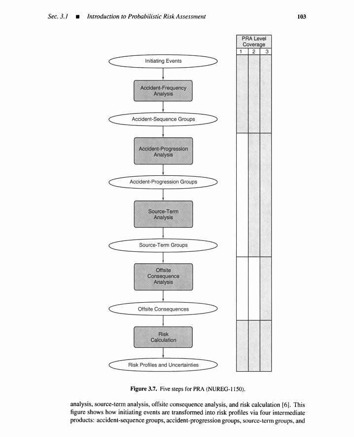
Sec.3.i • introduction to Probabilistic Risk Assessment 103
PRA LevelCoverage123
Initiating Eventsc -=::>
Accident-FrequencyAnalysis
Accident-Sequence Groups
Accident-ProgressionAnalys is
Accident-Progression Groups
Source-TermAnalysis
Source-Term Groups
OffsiteConsequence
Analysis
Offsite Consequences
RiskCalculation
Risk Protiles and Uncertainties
Figure 3.7. Five steps for PRA (NUREG-1150).
analysis, source-term analysis, offsite consequence analysis, and risk calculation [6]. Thisfigure shows how initiating events are transformed into risk profiles via four intermediateproducts: accident-sequence groups, accident-progression groups, source-term groups, and

104 Probabilistic Risk Assessment _ Chap. 3
offsite consequences.* Some steps can be omitted, depending on the application, but othersteps may have to be introduced. For instance, a collision accident scenario for passengertrains does not require a source-term analysis or offsite consequence analysis, but doesrequire an onsite consequence analysis to estimate passenger fatalities. Uncertainties in therisk profiles are evaluated by sampling likelihoods from distributions. t
3.1.6 Summary
PRA is a systematic method for transforming initiating events into risk profiles. Eventtrees coupled with fault trees are the kernel tools. PRAs for a passenger railway, a freightrailway, an ammonia storage facility, an oil tanker, and a nuclear power plant are presentedto emphasize that this methodology can apply to almost any plant or system for which riskmust be evaluated. A recent view of PRA is that it consists of five steps: 1) accident-frequency analysis, 2) accident-progression analysis, 3) source-term analysis, 4) offsiteconsequence analysis, and 5) risk calculation.
3.2 INITIATING-EVENT SEARCH
3.2.1 Searching for Initiating Events
Identification of initiating events (accident initiators) is an important task because riskprofiles can only be obtained through transformation of these events into consequences.Initiating events are any disruptions to normal plant operation that require automatic ormanual activation of plant safety systems. Initiating events due to failures of active andsupport systems are included. Thus a loss ofac power or cooling water becomes an initiatingevent. A full PRA deals with both internal and external initiating events.
A clear understanding of the general safety functions and features in the plant design,supplemented by a preliminary system review, provides the initial information necessary toselect and group initiating events [7].
Two approaches can be taken to identify initiating events.
1. The first is a general engineering evaluation, taking into consideration informationfrom previous risk assessments, documentation reflecting operating history, andplant-specific design data. The information is evaluated and a list of initiatingevents is compiled.
2. The second is a more formal approach. This includes checklists: preliminaryhazard analysis (PHA), failure mode and effects analysis (FMEA), hazard andoperability study (HAZOPS), or master logic diagrams (MLD). Although thesemethods (except for MLD) are not exclusively used for initiating-event identifica-tion, they are useful for identification purposes.
Initiating-event studies vary among industries and among companies. Unless specificgovernment regulations dictate the procedure, industrial practice and terminology will varywidely.
*In nuclear powerplant PRAs,accident-sequencegroups and accident-progressiongroupsare calledplant-damage states and accident-progression bins, respectively.
tUncertainty quantificationsare described in Chapter II.

Sec. 3.2 • Initiating-Event Search
3.2.2 Checklists
105
The only guideposts in achieving an understanding of initiators are sound engineeringjudgment and a detailed grasp of the environment, the process, and the equipment. Aknowledge of toxicity, safety regulations, explosive conditions, reactivity, corro siveness,and f1ammabilities is fundamental. Checklists such as the one used by Boeing Aircraft(shown in Figure 3.8) are a basic tool in identifying initiating events.
Hazardous Ene rgy Sources
1. Fuels 11. Gas Generators2. Propellants 12. Electrical Generators3. Initiators 13. Rapid·Fire Energy Sources4. Explosive Charges 14. Radioactive Energy Sources5. Charged Electrical Capacitors 15. Falling Objects6. Storage Batteries 16. Catapulted Objects7. Static Electrical Charges 17. Heating Devices8. Pressure Containers 18. Pumps, Blowers , Fans9. Spring-Loaded Devices 19. Rotating Machinery
10. Suspension Systems 20. Actuating Devices21. Nuclear Devices, etc.
Hazardous Process and Events
1. Accelerat ion 10. Moisture2. Contamination High Humidity3. Corrosion Low Humidity4. Chemical Dissociation 11. Oxidation5. Electricity 12. Pressure
Shock High PressureInadverten t Activation Low PressurePower Source Failure Rapid Pressure ChangesElectromagnetic Radiation 13. Radiation
6. Explosion Thermal7. Fire Electromagnetic8. Heat and Temperature Ionizing
High Temperature UltravioletLow Temperature 14. Chemical Replacement
9. Leakage 15. Mechanical Shock, etc.
Figure 3.8. Checklists of hazardous sources .
Initiating events lead to accidents in the form of uncontrollable releases of energy ortoxic materials. Certain parts of a plant are more likely to pose risks than others . Checklistsare used to identify uncontrollable releases (toxic release, explosion, fire, etc.) and todecompose the plant into subsystems to identify sections or components (chemical reactor,storage tank, etc .) that are likely sources of an accident or initiating event.
In looking for initiating events, it is necessary to bound the plant and the environmentunder study. It is not reasonable, for example, to include the probability of an airplanecrashing into a distillation column . However, airplane crashes, seismic risk, sabotage,adversary action, war, public utility failures, lightning, and other low-probability initiatorsdo enter into calculations for nuclear power plant risks because one can afford to protectagainst them and, theoretically, a nuclear power plant can kill more peop le than can adistillation column.

106 Probabilistic Risk Assessment _ Chap. 3
3.2.3 Preliminary Hazard Analysis
Hazards. An initiating event coupled with its potential consequence forms a haz-ard. If the checklist study is extended in a more formal (qualitative) manner to includeconsideration of the event sequences that transform an initiator into an accident, as well ascorrective measures and consequences of the accident, the study is a preliminary hazardanalysis.
In the aerospace industry, for example, the initiators, after they are identified, arecharacterized according to their effects. A common ranking scheme is
Class I Hazards:
Class II Hazards:
Class III Hazards:
Class IV Hazards:
Negligible effects
Marginal effects
Critical effects
Catastrophic effects
In the nuclear industry, Holloway classifies initiating events and consequences ac-cording to their annual frequenciesand severities,respectively[8]. The nth initiator groupsusually result in the nth consequence group if mitigation systems function successfully; aless frequent initiating event implies a more serious consequence. However, if mitigationsfail, the consequence group index may be higher than the initiator group index.
Initiator groups. These groups are classified according to annual frequencies.
1. IG1: O. 1 to 10 events per year.
2. IG2: 10-3 to 10- 1 events per year. These initiators are expected to be reasonably likely ina plant lifetime.
3. IG3: 10-5 to 10-3 events per year. These initiators often require reliably engineereddefenses.
4. IG4: 10-6 to 10-5 events per year. These initiators include light aircraft crashes and requiresome assurance of mitigation.
5. IGS: 10-7 to 10-6 events per year. These initiators include heavy aircraft crashes orprimary pressure vessel failure. Defenses are not required because of the low probabilitiesof occurrence.
Consequence groups. These groups, classified by severity of consequence, are
1. CG I: Trivial consequences expected as part of normal operation
2. CG2: Minor, repairable faults without radiological problems
3. CG3: Major repairable faults possibly with minor radiological problems
4. CG4: Unrepairable faults possibly with severe onsite and moderate offsite radiologicalproblems
5. CG5: Unrepairablefaults with major radiological releases
PHA tables. A common format for a PHA is an entry formulation such as shownin Tables 3.2 and 3.3. These are partially narrative in nature, listing both the events and the cor-rective actions that might be taken. During the process of making these tables, initiating events areidentified.
Column entries of Table 3.2 are defined as
1. Subsystem or function: Hardware or functional element being analyzed.
2. Mode: Applicable system phase or modes of operation.
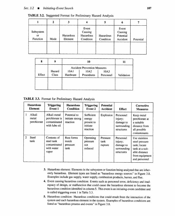
Sec. 3.2 • Initiating-Event Search
TABLE 3.2. Suggested Format for Preliminary Hazard Analysis
1 2 3 4 5 6 7
Event EventSubsystem Causing Causing
or Hazardous Hazardous Hazardous PotentialFunction Mode Element Condition Condition Accident Potential
8 9 10 11
Accident PreventionMeasuresHazard lOA! I IOA2 I IOA3
Effect Class Hardware Procedures Personnel Validation
TABLE 3.3. Format for Preliminary Hazard Analysis
107
Hazardous Triggering Hazardous Triggering Potential CorrectiveElement Event 1 Condition Event 2 Accident Effect Measures
I Alkali Alkali metal Potential to Sufficient Explosion Personnel Keep metalmetal perchlorate is initiate strong energy injury; perchlorate atperchlorate contaminated reaction present to damage to a suitable
with lube oil initiate surrounding distance fromreaction structures all possible
contaminants
2 Steel Contents of Rust forms Operating Pressure Personnel Use stainlesstank steel tank inside pressure tank injury; steel pressure
contaminated pressure not rupture damage to tank; locatewith water tank reduced surrounding tank at a suit-vapor structures able distance
from equipmentand personnel
3. Hazardous element: Elements in the subsystem or function being analyzed that are inher-ently hazardous. Element types are listed as "hazardous energy sources" in Figure 3.8.Examples include gas supply, water supply,combustion products, burner, and flue.
4. Event causing hazardous condition: Events such as personnel error, deficiency and inad-equacy of design, or malfunction that could cause the hazardous element to become thehazardouscondition identifiedin column 5. This event is an initiating-eventcandidate andis called triggering event 1 in Table 3.3.
5. Hazardous condition: Hazardous conditions that could result from the interaction of thesystem and each hazardous element in the system. Examples of hazardous conditions arelisted as "hazardous process and events" in Figure 3.8.
108 Probabilistic Risk Assessment _ Chap. 3
6. Eventcausingpotential accident: Undesired eventsor faultsthatcouldcausethehazardousconditionto becomethe identified potential accident. This event is called triggering event2 in Table3.3.
7. Potential accident: Anypotentialaccidentsthatcould result from the identified hazardousconditions.
8. Effect: Possibleeffectsof the potential accident,should it occur.
9. Hazardclass: Qualitative measureof significance for thepotentialeffectoneach identifiedhazardouscondition,according to the following criteria:
Class I (Safe)-Potential accidentsin column7 will not result in majordegradationand will not produceequipmentdamage or personnel injury.
Class II (Marginal)-Column 7 accidents will degrade performance but can becounteracted or controlledwithoutmajordamage or any injury to personnel.
ClassIII(Critical)-Theaccidentswilldegradeperformance, damageequipment,orresult in a hazardrequiringimmediate corrective action for personnel or equipmentsurvival.
Class IV (Catastrophic)-The accidents will severely degrade performance andcause subsequentequipment loss and/or death or multipleinjuries to personnel.
10. Accident-prevention measures: Recommended preventive measures toeliminateorcontrolidentified hazardous conditions and/or potential accidents. Preventive measures to berecommended should be hardwaredesign requirements, incorporation of safety devices,hardware design changes, special procedures, personnel requirements.
11. Record validated measures and keep aware of the status of the remaining recommendedpreventive measures. "Has the recommended solution been incorporated?" and "Is thesolutioneffective?" are the questionsansweredin validation. •
Support-system failures. Of particular importance in a PHA are equipment andsubsystem interface conditions. The interface is defined in MIL-STD-1629A as the sys-tems, external to the system beinganalyzed, that providea common boundaryor service andare necessaryfor the system to perform its mission in an undegradedmode(i.e., systems thatsupply power,cooling, heating, air services, or input signals are interfaces). Thus, an inter-face is nothing but a support system for the active systems. This emphasis on interfaces isconsistent with inclusionof initiatingevents involving support-systemfailures. Lambert [9]cites a classicexample thatoccurred in theearly stagesof ballisticmissiledevelopmentin theUnited States. Four major accidents occurred as the result of numerous interfaceproblems.In each accident, the loss of a multimillion-dollarmissile/silo launch complex resulted.
The failure of Apollo 13 was due to a subtle initiator in an interface (oxygen tank).During prelaunch, improper voltage was applied to the thermostatic switches leading to theheater of oxygen tank #2. This caused insulation on the wires to a fan inside the tank tocrack. During flight, the switch to the fan was turned on, a short circuit resulted, it causedthe insulation to ignite and, in tum, caused the oxygen tank to explode.
In general, a PHA represents a first attempt to identify the initiators that lead toaccidents while the plant is still in a preliminary design stage. Detailed event analysis iscommonly done by FMEA after the plant is fully defined.
3.2.4 Failure Mode and Effects Analysis
This isan inductiveanalysisthatsystematicallydetails, onacomponent-by-componentbasis, all possible failure modes and identifiestheir resulting effects on the plant [10]. Pos-sible single modes of failure or malfunctionof each component in a plant are identifiedandanalyzed to determine their effect on surrounding components and the plant.

Sec.3.2 • Initiating-Event Search 109
Failure modes. This technique is used to perform single-random-failure analysisas required by IEEE Standard 279-1971, 10 CFR 50, Appendix K, and regulatory guide1.70, Revision 2. FMEA considers every mode of failure of every component. A relay, forexample, can fail by [11]:
contacts stuck closedcontacts slow in openingcontacts stuck opencontacts slow in closingcontact short circuit
to groundto supplybetween contactsto signal lines
contacts chatteringcontacts arcing, generating noisecoil open circuitcoil short circuit
to supplyto contactsto groundto signal lines
coil resistancelowhigh
coil overheatingcoil overmagnetized or excessive hysteresis (same effect as contacts stuck closed or slow
in opening)Generic failure modes are listed in Table 3.4 [12].
TABLE 3.4. Generic Failure Modes
No. Failure Mode No. Failure Mode
1 Structural failure (rupture) 19 Fails to stop2 Physical binding or jamming 20 Fails to start3 Vibration 21 Fails to switch4 Fails to remain (in position) 22 Premature operation5 Fails to open 23 Delayed operation6 Fails to close 24 Erroneous input (increased)7 Fails open 25 Erroneous input (decreased)8 Fails closed 26 Erroneous output (increased)9 Internal leakage 27 Erroneous output (decreased)
10 External leakage 28 Loss of input11 Fails out of tolerance (high) 29 Loss of output12 Fails out of tolerance (low) 30 Shorted (electrical)13 Inadvertent operation 31 Open (electrical)14 Intermittent operation 32 Leakage (electrical)15 Erratic operation 33 Other unique failure condition16 Erroneous indication as applicable to the system17 Restricted flow characteristics, requirements18 False actuation and operational constraints

110 Probabilistic Risk Assessment _ Chap. 3
Checklists. Checklists for each category of equipment must also be devised. Fortanks, vessels, and pipe sections, a possible checklist is
1. Variables: flow, quantity, temperature, pressure, pH, saturation.
2. Services: heating, cooling, electricity, water, air, control, N2•
3. Special states: maintenance, start-up, shutdown, catalyst change.
4. Changes: too much, too little, none, water hammer, nonmixing, deposit, drift, os-cillation, pulse, fire, drop, crash, corrosion, rupture, leak, explosion, wear, openingby operator, overflow.
S. Instrument: sensitivity, placing, response time.
Table 3.5 offers a format for the FMEA. This format is similar to those used in apreliminary hazard analysis, the primary difference being the greater specificity and degreeof resolution of the FMEA (which is done after initial plant designs are completed).
3.2.5 FMECA
Criticality analysis (CA) is an obvious next step after an FMEA. The combination iscalled an FMECA-failure mode and effects and criticality analysis. CA is a procedure bywhich each potential failure mode is ranked according to the combined influence of severityand probability of OCCUITence.
Severity and criticality. In both Tables 3.3 and 3.5, each effect is labeled withrespect to its critical importance to mission operation. According to MIL-STD-1629A,severity and criticality are defined as follows [10,] 3].
1. Severity: The consequences of a failure mode. Severity considers the worst poten-tial consequence of a failure, determined by the degree of injury, property damage,or system damage that ultimately occurs.
2. Criticality: A relative measure of the consequences of a failure mode and itsfrequency of occurrences.
As with the consequence groups for the PHA used to rank initiating events, severityfor FMECA is rated in more than one way and for more than one purpose.
Severity classification. MIL-STD-1629A recommends the following severity clas-sification.
1. Category I: Catastrophic-A failure that may cause death or weapon system loss(i.e., aircraft, tank, missile, ship, etc.)
2. Category 2: Critical-A failure that may cause severe injury, major propertydamage, or major system damage that results in mission loss.
3. Category 3: Marginal-A failure that may cause minor injury, minor propertydamage, or minor system damage that results in delay or loss of availability ormission degradation.
4. Category 4: Minor-A failure not serious enough to cause injury, property damage,or system damage, but that results in unscheduled maintenance or repair.
Multiple-failure-mode probability levels. Denote by P a single-failure-mode prob-ability for a component during operation. Denote by Po an overall component failureprobability during operation. Note that the overall probability includes all failure modes.
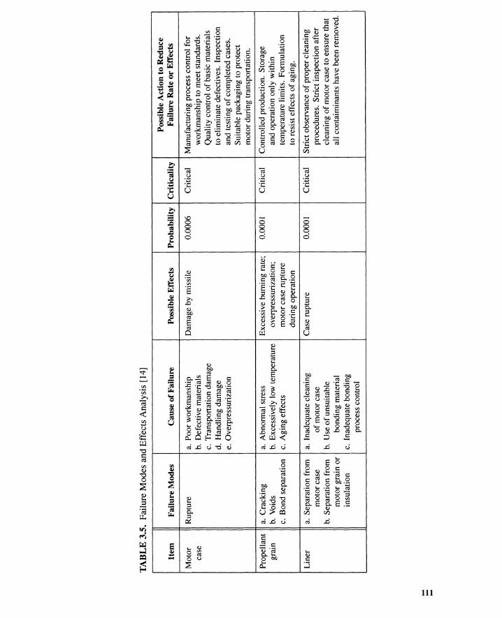
~ ~ ~
TA
BL
E3.
5.Fa
ilure
Mod
esan
dE
ffec
tsA
naly
sis
[14]
Poss
ible
Act
ion
toR
educ
eIt
emF
ailu
reM
odes
Cau
seof
Fai
lure
Poss
ible
Eff
ects
Pro
babi
lity
Cri
tica
lity
Fai
lure
Rat
eo
rE
ffec
ts
Mot
orR
uptu
rea.
Poo
rw
orkm
ansh
ipD
amag
eby
mis
sile
0.00
06C
riti
cal
Man
ufac
turi
ngpr
oces
sco
ntro
lfo
rca
seb.
Def
ecti
vem
ater
ials
wor
kman
ship
tom
eet
stan
dard
s.c.
Tra
nspo
rtat
ion
dam
age
Qua
lity
cont
rol
ofba
sic
mat
eria
lsd.
Han
dlin
gda
mag
eto
elim
inat
ede
fect
ives
.In
spec
tion
e.O
verp
ress
uriz
atio
nan
dte
stin
go
fcom
plet
edca
ses.
Sui
tabl
epa
ckag
ing
topr
otec
tm
otor
duri
ngtr
ansp
orta
tion
.
Pro
pell
ant
a.C
rack
ing
a.A
bnor
mal
stre
ssE
xces
sive
burn
ing
rate
;0.
0001
Cri
tica
lC
ontr
olle
dpr
oduc
tion
.S
tora
gegr
ain
b.V
oids
b.E
xces
sive
lylo
wte
mpe
ratu
reov
erpr
essu
riza
tion
;an
dop
erat
ion
only
wit
hin
c.B
ond
sepa
rati
onc.
Agi
ngef
fect
sm
otor
case
rupt
ure
tem
pera
ture
limits
.F
orm
ulat
ion
duri
ngop
erat
ion
tore
sist
effe
cts
ofag
ing.
Lin
era.
Sep
arat
ion
from
a.In
adeq
uate
clea
ning
Cas
eru
ptur
e0.
0001
Cri
tica
lS
tric
t obs
erva
nce
ofpr
oper
clea
ning
mot
orca
seof
mot
orca
sepr
oced
ures
.S
tric
tin
spec
tion
afte
rb.
Sep
arat
ion
from
b.U
seof
unsu
itab
lecl
eani
ngof
mot
orca
seto
ensu
reth
atm
otor
grai
nor
bond
ing
mat
eria
lal
lco
ntai
min
ants
have
been
rem
oved
.in
sula
tion
c.In
adeq
uate
bond
ing
proc
ess
cont
rol

112 Probabilistic Risk ASSeSSI11ent _ Chap. 3
Qualitative levels for probability P are dependent on what fraction of Po the failure modeoccupies. In other words, each level reflects a conditional probability of a failure mode,given a component failure.
1. Level A-Frequent: 0.20Po < P
2. Level B-Reasonably probable: O.IOPo < P :s 0.20Po3. Level C-Occasional: 0.0 I Po < P :s 0.1OPo4. Level D-Remote: 0.001 Po < P :s 0.01 Po
5. Level E-Extremely unlikely: P :s 0.001 Po
Failure-mode criticality number. Consider a particular severity classification scfor system failures. A ranking of failure mode In for severity classification purposes can beachieved by computing criticality number Cm,sc (see Figure 3.9). This criticality numberCm,sc is the number of system failures falling in severity classification sc per hour or trialcaused by component failure mode 111.
where
Cm.sc == fJscCtAp
== fJsc Ct AbJrAn E
(3.1)
(3.2)
1. Cm.sc == criticality number for failure mode 111, given severity classification sc forsystem failure.
2. fJsc == failure effect probability. The fJsc values are the conditional probabilities thatthe failure effect results in the identified severity classification sc, given that thefailure mode occurs. Values of fJ.\'C are selected from an established set of ranges:
Analyst's Judgment
Actual effectProbable effectPossible effectNone
Typical Value of f3sc
f3sc = 1.000.01 < f3sc < 1.000.00 < f3sc ~ 0.01e; = 0.00
3. a == failure mode ratio. This is the probability expressed as a decimal fractionthat the component fails in the identified mode. If all potential failure modes of acomponent are listed, the sum of the a values for that component equals one.
4. Ap == component failure rate in failures per hour or trial.Component failure rate Ap is calculated by
(3.3)
where
5. Ab == component basic failure rate in failures per hour or trial that is obtained, forinstance, from MIL-HDBK-217.
6. n A == application factor that adjusts Ab for the difference between operating stressesunder which Ab was measured and the operating stresses under which the compo-nent is used.
7. n E == environmental factor that adjusts Ab for differences between environmentalstresses under which Ab was measured and the environmental stresses under whichthe component is going to be used.

Sec. 3.2 • Initiating-Event Search 113
SystemFailureSeverityClasssc
Figure 3.9. Calculation of criticality number em.se •
As a result, the failure-mode criticality number Cm,sc is represented by:
Cm,sc == fJscCXAb TC ATCE (3.4)
Component criticality number. Assume a total number of n failure modes for acomponent. For each severity classification sc, component criticality number Csc is
m=n
c; == L c.:m=l
(3.5)
The component criticality number Csc is the number of system failures in severityclassification sc per hour or trial caused by the component. Note that m denotes a particularcomponent failure mode, sc is a specific severity classification for system failures, and n isa total number of failure modes for the component.
Note that this ranking method places value on possible consequences or damagethrough severity classification sc. Besides being useful for initiating event identification asa component failure mode, criticality analysis is useful for achieving system upgrades byidentifying [14]
1. which components should be given more intensive study for elimination of thehazard, and for fail-safe design, failure-rate reduction, or damage containment.
2. which components require special attention during production, require tight qualitycontrol, and need protective handling at all times.
3. special requirements to be included in specifications for suppliers concerning de-sign, performance, reliability, safety, or quality assurance.
4. acceptance standards to be established for components received at a plant fromsubcontractors and for parameters that should be tested intensively.
5. where special procedures, safeguards, protective equipment, monitoring devices,or warning systems should be provided.
6. where accident prevention efforts and funds could be applied most effectively.This is especially important, since every program is limited by the availability offunds.
3.2.6 Hazard and Operability Study
Guide words. In identifying subsystems of the plant that give rise to an accidentinitiator, it is useful to list guide words that stimulate the exercise of creative thinking. AHAZOPS [15-19] suggests looking at a process to see how it might deviate from designintent by applying the following guide words.
More ofNone ofLater thanReverseOther than
Less ofPart ofSooner thanWrong AddressAs well as
Examples of process parameter deviations are listed in Table 3.6 [18].

114 Probabilistic Risk Assessment _ Chap. 3
TABLE 3.6. Process Parameter Deviations for HAZOP
Process Parameter Deviation
Flow No flowReverse flowMore flowExtra flowChange in flow proportionsFlow to wrong place
Temperature Higher temperatureLower temperature
Pressure Higher pressureLower pressure
Volume Higher level (in a tank)Lower level (in a tank)Volume rate changes faster than expectedProportion of volumes is changed
Composition More component ALess component BMissing component CComposition changed
pH Higher pHLower pHFaster change in pH
Viscosity Higher viscosityLower viscosity
Phase Wrong phaseExtra phase
HAZOPS and FMEA. In a sense, a HAZOPS is an extended FMEA technique,the extension being in the direction of including process parameter deviations in additionto equipment failure modes. Any potential hazards or operability problems (e.g., loss ofautomatic control) are explored as consequences of such deviations. This can also be usedfor initiating-event identification.
The use of HAZOPS technique at the Imperial Chemical Industries is described asfollows.
HAZOPS is a detailed failure mode and effect analysis of the Piping and Instrument (P & I)line diagram. A team of four or five people study the P & I line diagram in formal andsystematical manner. The team includes the process engineer responsible for the chemicalengineeringdesign; the projectengineer responsiblefor the mechanicalengineeringdesign andhavingcontrol of the budget; the commissioning manager who has the greatest commitment tomaking the plant a good one and who is usually appointed at a very early stage of the projectdesign; a hazard analyst who guides the team through the hazard study and quantifiesany risksas necessary.

Sec. 3.2 • Initiating-Event Search 115
This team studieseach individual pipe and vessel in turn, using a series of guide wordsto stimulatecreativethinkingabout what wouldhappenif the fluid in the pipe were to deviatefrom the design intentionin any way. The guide wordswhich we use for continuouschemicalplantsincludehighflow, lowflow, no flow, reverseflow, highand lowtemperature andpressureand any other deviationof a parameterof importance. Maintenance, commissioning, testing,start-up, shutdown and failure of servicesare also consideredfor each pipe and vessel.
This in-depth investigation of the line diagram is a key feature of the whole projectand obviously takes a lot of time-about 200 man hours per $2,000,000 capital. It is verydemanding and studies, each lasting about 2.5 hours, can only be carried out at a rate ofabout two or three per week. On a multimillion dollar project, therefore, the studies couldextend over many weeks or months. Problems identified by the hazard study team are re-ferred to appropriatemembers of team or to experts in support groups. If, during the courseof this study, we uncover a major hazard which necessitates some fundamental redesign orchange in design concept, the study will be repeated on the redesigned line diagram. Manyoperability, maintenance, start-up and shutdown problemsare identified and dealt with satis-factorily.
Computerized versions of HAZOPS and FMEA are described in [19,20].
3.2.7 Master Logic Diagram
A fault-tree-based PRA uses a divide-and-conquer strategy, where an accident is de-composed into subgroups characterized by initiating events, and this is further decomposedinto accident sequences characterized by the event-tree headings. For each initiating eventor event-tree heading, a fault tree is constructed. This divide-and-conquer strategy is lesssuccessful if some initiating events are overlooked. An MLD uses the fault trees to searchfor accident initiators.
An example of an MLD for a nuclear power plant is shown in Figure 3.10 [7]. Thetop event on the first level in the diagram represents the undesired event for which the PRAis being conducted, that is, an excessive offsite release of radionuclides. This top event issuccessively refined by levels. The OR gate on level 2 answers the question, "How can arelease to the environment occur?" yielding "Release of core material" and "Release ofnoncore material." The AND gate on level 3 shows that a release of radioactive materialrequires simultaneous core damage and containment failure. The OR gate on level 4 below"Core damage" answers the question, "How can core damage occur?" After several morelevels of "how can" questions, the diagram arrives at a set of potential initiating events,which are hardware or people failures.
A total of 59 internal initiating events were eventually found by MLD for the sce-nario partly shown in Figure 3.10. These events are further grouped according to miti-gating system requirements. The NUREG-1150 PRA was able to reduce the number ofinitiating-event categories by combining several that had the same plant response. Forexample, the loss of steam inside and outside the containment was collapsed into lossof steam, resulting in a reduction of the initiating event categories for the NUREG-1150analysis.
3.2.8 Summary
Initiating-event identification is a most important PRA task because accidents haveinitiators. The following approaches can be used for identification: checklists; preliminary
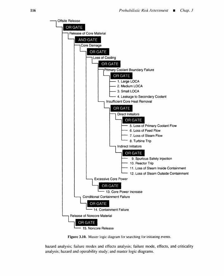
116 Probabilistic Risk Assessment _ Chap. 3
Offsite Release-Release of Core Material
AND GATE
Core Damage--Loss of Cooling-Primary Coolant Boundary Failure-1. Large LOCA
2. Medium LOCA
3. Small LOCA
4. Leakage to Secondary Coolant
Insufficient Core Heat Removal-Direct Initiators-5. Loss of Primary Coolant Flow
6. Loss of Feed Flow
7. Loss of Steam Flow
8. Turbine Trip
Indirect Initiators-9. Spurious Safety Injection10. Reactor Trip
11. Loss of Steam Inside Containment
12. Loss of Steam Outside Containment
Excessive Core Power
13. Core Power Increase
Conditional Containment Failure
14. Containment Failure
Release of Noncore Material-15. Noncore Release
Figure 3.10. Master logic diagram for searching for initiating events.
hazard analysis; failure modes and effects analysis; failure mode, effects, and criticalityanalysis; hazard and operability study; and master logic diagrams.

Sec. 3.3 • The Three PRA Levels
3.3 THE THREE PRA LEVELS
117
As shown by the "PRA Level Coverage" in Figure 3.7, a level 1 PRA consists of the first andlast of the five PRA steps, that is, accident-frequency analysis and risk calculation. A level2 PRA performs accident-progression and source-term analyses in addition to the level 1PRA analyses. A level 3 PRA performs a total of five analyses, that is, an offsite conse-quence analysis and level 2 PRA analyses. Each PRA performs risk calculations. Level1 risk profiles refer to accident occurrence, level 2 profiles to material release magnitudes,and level 3 profiles to consequence measures such as fatalities.
3.3.1 Leve/1 PRA-Accident Frequency
This PRA mainly deals with accident frequencies, that is, frequencies of core damage,train collisions, oil tanker groundings, and so forth. Accident sequences and their groups areidentified in a level 1 PRA. The plant states associated with these accident-sequence groupsare core damage by melting, train damage by collision, oil tanker damage by grounding,and so on. These accident-sequence groups are used as inputs to a level 2 PRA.
3.3.1.1 Accident-frequency analysis. A level 1PRA analyzes how initiating eventsdevelop into accidents. This transformation is called an accident- frequency analysis in PRAterminology. Level 1 PRAs identify combinations of events that can lead to accidents andthen estimate their frequency of occurrence. The definition of accident varies from appli-cation to application. Some applications involve more than one accident. For instance, fora railway it may include collision and derailment. Initiating events also differ for differentapplications. A loss of coolant is an initiating event for a nuclear power plant, while anunscheduled departure is an accident initiator for a railway collision.
A level 1 PRA consists of the activities shown in Figure 3.11.
1. Initiating-event analysis (see Section 3.3.1.3).
2. Event-tree construction (see Section 3.3.1.4).
3. Fault-tree construction (see Section 3.3.1.5).
4. Accident-sequence screening (see Section 3.3.1.6).
5. Accident-sequence quantification (see Section 3.3.1.6).
6. Grouping of accident sequences (see Section 3.3.1.10).
7. Uncertainty analysis (see Section 3.3.1.11).
These activities are supported by the following analyses.
1. Plant-familiarization analysis (see Section 3.3.1.2).
2. Dependent-failure analysis (see Section 3.3.1.7).
3. Human-reliability analysis (see Section 3.3.1.8).
4. Database analysis (see Section 3.3.1.9).
This section overviews these activities.
3.3.1.2 Plant-familiarization analysis. An initial PRA task is to gain familiaritywith the plant under investigation, as a foundation for subsequent tasks. Information is as-sembled from such sources as safety analysis reports, piping and instrumentation diagrams,
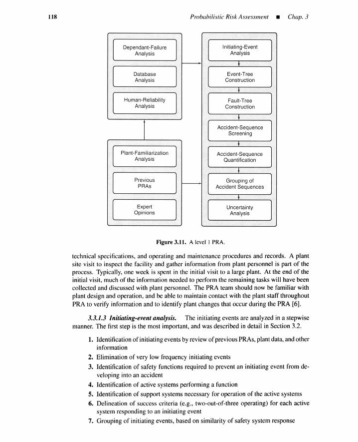
118 Probabilist ic Risk Assessment • Chap. 3
Dependant-Failure Initiating- EventAnalysis Analysis
l
Database Event-TreeAnalys is Construction
~
Human-Reliability Fault-TreeAnalysis Construction
~
Accident-SequenceScreening
l
Plant-Familiarization Acc ident -Seque nceAnalysis Quantification
~
Previous Grouping ofPRAs Accident Sequences
l
Expert UncertaintyOpinions Analysis
Figure 3.11. A level I PRA.
technical specifications, and operating and maintenance procedures and records. A plantsite visit to inspect the facility and gather information from plant personnel is part of theprocess. Typically, one week is spent in the initial visit to a large plant. At the end of theinitial visit, much of the information needed to perform the remaining tasks will have beencollected and discussed with plant personnel. The PRA team should now be familiar withplant design and operation, and be able to maintain contact with the plant staff throughoutPRA to verify information and to identify plant changes that occur during the PRA [6].
3.3.1.3 Initiating-event analysis. The initiating events are analyzed in a stepwisemanner. The first step is the most important, and was described in detail in Section 3.2.
1. Identification of initiating events by review of previous PRAs, plant data, and otherinformation
2. Elimination of very low frequency initiating events
3. Identification of safety functions required to prevent an initiating event from de-veloping into an accident
4. Identification of active systems performing a function
5. Identification of support systems necessary for operation of the active systems
6. Delineation of success criteria (e.g., two-out-of-three operating) for each activesystem responding to an initiating event
7. Grouping of initiating events, based on similarity of safety system response

Sec. 3.3 • The Three PRA Levels 119
Initiating-event and operation mode. For a nuclear power plant, a list of initiatingevents is available in NUREG-1150. These include LOCA, support-system initiators, andother transients. Different sets of initiating events may apply to modes of operation such asfull power, low power (e.g., up to 15% power), start-up, and shutdown. The shutdown modeis further divided into cold shutdown, hot shutdown, refueling, and so on. An inadvertentpower increase at low power may produce a plant response different from that at fullpower [21].
Grouping ofinitiating events. For each initiating event, an event tree is developedthat details the relationships among the systems required to respond to the event, in terms ofpotential system successes and failures. For instance, the event tree of Figure 3.2 considersan unscheduled departure of terminal A train when another train is between terminal Bandspur signal 3. If more than one initiating event is involved, these events are examined andgrouped according to the mitigation system response required. An event tree is developedfor each group of initiating events, thus minimizing the number of event trees required.
3.3.1.4 Event-tree construction
Event trees coupled with fault trees. Event trees for a level 1 PRA are calledaccident-sequence event trees. Active systems and related support systems in event-treeheadings are modeled by fault trees. Boolean logic expressions, reliability block diagrams,and other schematics are sometimes used to model these systems. A combination of eventtrees and fault trees is illustrated in Figure 1.10 where the initiating event is a pump overrunand the accident is a tank rupture. Figure 3.2 is another example of an accident-sequenceevent tree where the unscheduled departure is an initiating event. This initiator can also beanalyzed by a fault tree that should identify, as a cause of the top event, the human errorof neglecting a red departure signal because of heavy traffic. The departure-monitoringsystem failure can be analyzed by a fault tree that deduces basic causes such as an electronicinterface failure because of a maintenance error. The cause-consequence diagram describedin Chapter 1 is an extension of this marriage of event and fault trees.
Event trees enumerate sequences leading to an accident for a given initiating event.Event trees are constructed in a step-by-step process. Generally, a function event tree iscreated first. This tree is then converted into a system event tree. Two approaches areavailable for the marriage of event and fault trees: large ET/small FT approach, and smallET/large FT approach.
Function event trees. Initiating events are grouped according to safety system re-sponses; therefore, construction focuses on safety system functions. For the single trackrailway problem, the safety functions include departure monitoring and spur signal watch-ing. The first function is performed either by an automatic departure monitoring device orby a human.
A nuclear power plant has the following safety functions [7]. The same safety functioncan be performed by two or more safety systems.
1. Reactivity control: shuts reactor down to reduce heat production.
2. Coolant inventory control: maintains a coolant medium around the core.
3. Coolant pressure control: maintains the coolant in its proper state.
4. Core-heat removal: transfers heat from the core to a coolant.
5. Coolant-heat removal: transfers heat from the coolant.
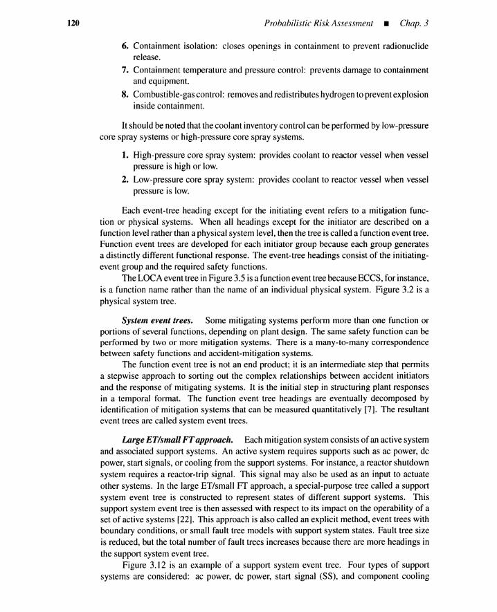
120 Probabilistic Risk Assessment _ Chap. 3
6. Containment isolation: closes openings in containment to prevent radionucliderelease.
7. Containment temperature and pressure control: prevents damage to containmentand equipment.
8. Combustible-gascontrol: removesand redistributeshydrogento preventexplosioninside containment.
It should be noted that thecoolant inventory controlcan be performedby low-pressurecore spray systems or high-pressure core spray systems.
1. High-pressure core spray system: provides coolant to reactor vessel when vesselpressure is high or low.
2. Low-pressure core spray system: provides coolant to reactor vessel when vesselpressure is low.
Each event-tree heading except for the initiating event refers to a mitigation func-tion or physical systems. When all headings except for the initiator are described on afunction levelrather than a physicalsystem level, then the tree is called a functionevent tree.Function event trees are developed for each initiator group because each group generatesa distinctly different functional response. The event-tree headings consist of the initiating-event group and the required safety functions.
The LOCAevent tree inFigure 3.5 isa functionevent treebecauseECCS, for instance,is a function name rather than the name of an individual physical system. Figure 3.2 is aphysical system tree.
System event trees. Some mitigating systems perform more than one function orportions of several functions, depending on plant design. The same safety function can beperformed by two or more mitigation systems. There is a many-to-many correspondencebetween safety functions and accident-mitigationsystems.
The function event tree is not an end product; it is an intermediate step that permitsa stepwise approach to sorting out the complex relationships between accident initiatorsand the response of mitigating systems. It is the initial step in structuring plant responsesin a temporal format. The function event tree headings are eventually decomposed byidentification of mitigation systems that can be measured quantitatively [7]. The resultantevent trees are called system event trees.
Large ET/small FTapproach. Each mitigationsystemconsistsof an activesystemand associated support systems. An active system requires supports such as ac power, depower, start signals, or cooling from the support systems. For instance, a reactor shutdownsystem requires a reactor-trip signal. This signal may also be used as an input to actuateother systems. In the large ET/small FT approach, a special-purpose tree called a supportsystem event tree is constructed to represent states of different support systems. Thissupport system event tree is then assessed with respect to its impact on the operability of aset of active systems [22]. This approach is also called an explicit method, event trees withboundary conditions, or small fault tree models with support system states. Fault tree sizeis reduced, but the total number of fault trees increases because there are more headings inthe support system event tree.
Figure 3.12 is an example of a support system event tree. Four types of supportsystems are considered: ac power, dc power, start signal (SS), and component cooling
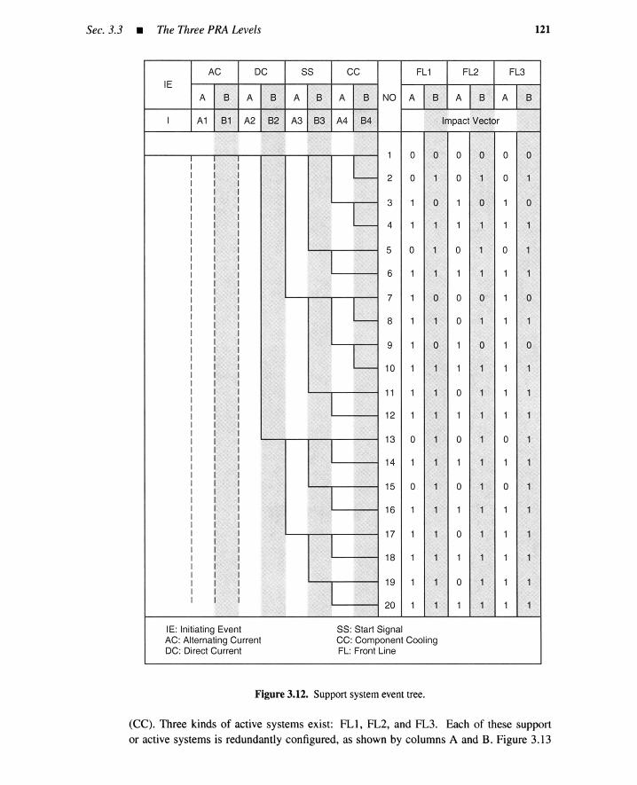
Sec. 3.3 • The Three PRA Levels 121
AC DC SS CC FL1 FL2 FL3IE
A 8 A 8 A 8 A 8 NO A 8 A 8 A 8
I A1 81 A2 82 A3 83 A4 84 Impact Vector
1 0 0 0 0 0 0I I
L 2 0 1 0 1 0 1
3 1 0 1 0 1 0
L 4 1 1 1 1 1 1
5 0 1 0 1 0 1
6 1 1 1 1 1 1
7 1 0 0 0 1 0
L 8 1 1 0 1 1 1
9 1 0 1 0 1 0
L 10 1 1 1 1 1 1
11 1 1 0 1 1 1
12 1 1 1 1 1 1
13 0 1 0 1 0 1
14 1 1 1 1 1 1
15 0 1 0 1 0 1
II 16 1 1 1 1 1 1III 17 1 1 0 1 1 1III 18 1 1 1 1 1 1III 19 1 1 0 1 1 1II
20 1 1 1 1 1 1
IE: Initiating Event SS: Start SignalAC: Alternating Current CC: Component CoolingDC: Direct Current FL: Front Line
Figure 3.12. Supportsystem event tree.
(CC) . Three kinds of active systems exist: FLl , FL2, and FL3. Each of these support
or active systems is redundantly configured, as shown by columns A and B. Figure 3.13
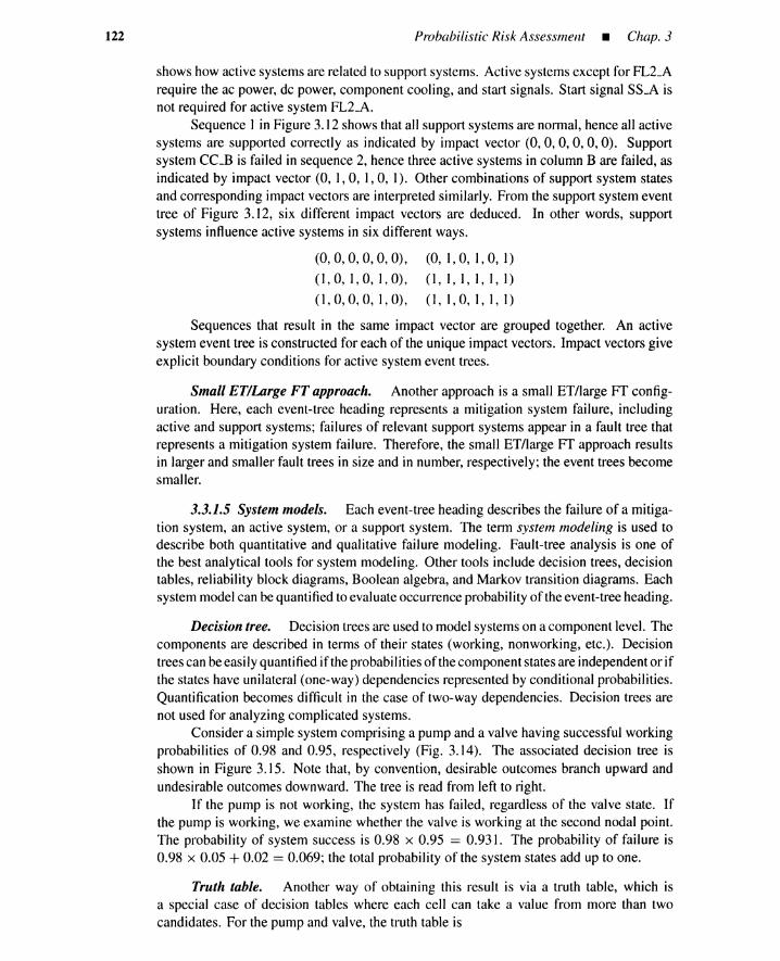
122 Probabilistic Risk Assessment _ Chap. 3
shows how active systems are related to support systems. Active systems except for FL2_Arequire the ac power, de power, component cooling, and start signals. Start signal SS_A isnot required for active system FL2_A.
Sequence I in Figure 3.12 shows that all support systems are normal, hence all activesystems are supported correctly as indicated by impact vector (0,0,0,0,0,0). Supportsystem CC_B is failed in sequence 2, hence three active systems in column B are failed, asindicated by impact vector (0, 1, 0, 1, 0, 1). Other combinations of support system statesand corresponding impact vectors are interpreted similarly. From the support system eventtree of Figure 3.12, six different impact vectors are deduced. In other words, supportsystems influence active systems in six different ways.
(0,0,0,0, 0, 0),
(1,0,1,0, 1,0),
(1,0,0,0,1,0),
(0, 1,0, I, 0, I)
(I, I, I, I, I, I)
(I, 1,0, I, 1, I)
Sequences that result in the same impact vector are grouped together. An activesystem event tree is constructed for each of the unique impact vectors. Impact vectors giveexplicit boundary conditions for active system event trees.
Small ET/Large FT approach. Another approach is a small ET/large FT config-uration. Here, each event-tree heading represents a mitigation system failure, includingactive and support systems; failures of relevant support systems appear in a fault tree thatrepresents a mitigation system failure. Therefore, the small ET/large FT approach resultsin larger and smaller fault trees in size and in number, respectively; the event trees becomesmaller.
3.3.1.5 System models. Each event-tree heading describes the failure of a mitiga-tion system, an active system, or a support system. The term system modeling is used todescribe both quantitative and qualitative failure modeling. Fault-tree analysis is one ofthe best analytical tools for system modeling. Other tools include decision trees, decisiontables, reliability block diagrams, Boolean algebra, and Markov transition diagrams. Eachsystem model can be quantified to evaluate occurrence probability of the event-tree heading.
Decision tree. Decision trees are used to model systems on a component level. Thecomponents are described in terms of their states (working, nonworking, etc.). Decisiontrees can be easily quantified if the probabilities of the component states are independent or ifthe states have unilateral (one-way) dependencies represented by conditional probabilities.Quantification becomes difficult in the case of two-way dependencies. Decision trees arenot used for analyzing complicated systems.
Consider a simple system comprising a pump and a valve having successful workingprobabilities of 0.98 and 0.95, respectively (Fig. 3.14). The associated decision tree isshown in Figure 3.15. Note that, by convention, desirable outcomes branch upward andundesirable outcomes downward. The tree is read from left to right.
If the pump is not working, the system has failed, regardless of the valve state. Ifthe pump is working, we examine whether the valve is working at the second nodal point.The probability of system success is 0.98 x 0.95 == 0.931. The probability of failure is0.98 x 0.05 + 0.02 == 0.069; the total probability of the system states add up to one.
Truth table. Another way of obtaining this result is via a truth table, which isa special case of decision tables where each cell can take a value from more than twocandidates. For the pump and valve, the truth table is
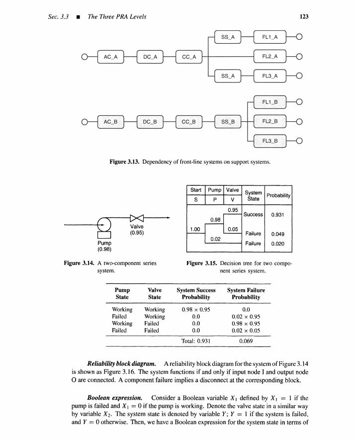
Sec. 3.3 • The Three PRA Levels 123
Figure 3.13. Dependency of front-line systems on support systems.
B[><]Valve(0.95)
Pump(0.98)
Figure 3.14. A two-component seriessystem.
Start Pump Valve SystemS P V State
Probability
0.95r- Success 0.931
0.98r--
1.00 0.05r-- '-- Failure 0.049
0.02Failure 0.020
Figure 3.15. Decision tree for two compo-nent series system.
Pump Valve System Success System FailureState State Probability Probability
Working Working 0.98 x 0.95 0.0Failed Working 0.0 0.02 x 0.95Working Failed 0.0 0.98 x 0.95Failed Failed 0.0 0.02 x 0.05
Total: 0.931 0.069
Reliability block diagram. A reliability block diagram for the system of Figure 3.14is shown as Figure 3.16. The system functions if and only if input node I and output nodeo are connected. A component failure implies a disconnect at the corresponding block.
Boolean expression. Consider a Boolean variable X I defined by X I = I if thepump is failed and Xl = 0 if the pump is working. Denote the valve state in a similar wayby variable X2. The system state is denoted by variable Y; Y = I if the system is failed,and Y = 0 otherwise. Then, we have a Boolean expression for the system state in terms of
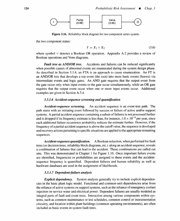
124 Probabilistic Risk Assessment _ Chap. 3
Figure 3.16. Reliabilityblockdiagram for two componentseries system.
the two component states:
(3.6)
where symbol v denotes a Boolean OR operation. Appendix A.2 provides a review ofBoolean operations and Venn diagrams.
Fault tree as AND/OR tree. Accidents and failures can be reduced significantlywhen possible causes of abnormal events are enumerated during the system design phase.As described in Section 3.1.4, an FTA is an approach to cause enumeration. An Ff isan AND/OR tree that develops a top event (the root) into more basic events (leaves) viaintermediate events and logic gates. An AND gate requires that the output event fromthe gate occur only when input events to the gate occur simultaneously, while an OR gaterequires that the output event occur when one or more input events occur. Additionalexamples are given in Section A.3.4.
3.3.1.6 Accident-sequence screening and quantification
Accident-sequence screening. An accident sequence is an event-tree path. Thepath starts with an initiating event followed by success or failure of active and/or supportsystems. A partial accident sequence containing a subset of failures is not processed furtherand is dropped if its frequency estimate is less than, for instance, 1.0 x 10⁻⁹ per year, sinceeach additional failure occurrence probability reduces the estimate further. However, if thefrequency of a partial accident sequence is above the cutoff value, the sequence is developedand recoveryactions pertaining tospecificsituationsare applied to the appropriateremainingsequences.
Accident-sequence quantification. A Boolean reduction, whenperformed for faulttrees (or decision trees, reliability block diagrams, etc.) along an accident sequence, revealsa combination of failures that can lead to the accident. These combinations are called cutsets. This was demonstrated in Chapter I for Figure 1.10. Once important failure eventsare identified, frequencies or probabilities are assigned to these events and the accident-sequence frequency is quantified. Dependent failures and human reliability as well ashardware databases are used in the assignment of likelihoods.
3.3.1.7 Dependent-failure analysis
Explicit dependency. System analysts generally try to include explicit dependen-cies in the basic plant logic model. Functional and common-unit dependencies arise fromthe reliance of active systems on support systems, such as the reliance of emergency coolantinjection on service water and electrical power. Dependent failures are usually modeled asintegral parts of fault and event trees. Interaction among various components within sys-tems, such as common maintenance or test schedules, common control or instrumentationcircuitry, and location within plant buildings (common operating environments), are oftenincluded as basic events in system fault trees.

Sec. 3.3 • The Three PRA Levels 125
Implicit dependency. Even though the fault- and event-tree models explicitly in-clude major dependencies, in some cases it is not possible to identify the specific mecha-nisms of a common-cause failure from available databases. In other cases, there are manydifferent types of common-cause failures, each with a low probability, and it is not practicalto model them separately. Parametric models (see Chapter 9) can be used to account for thecollective contribution of residual common-cause failures to system or component failurerates.
3.3.1.8 Human-reliability analysis. Human-reliability analysis identifies humanactions in the PRA process.* It also determines the human-error rates to be used in quan-tifying these actions. The NUREG-1150 analysis considers pre-initiator human errors thatoccur before an initiating event (inclusive), and post-initiator human errors after the initi-ating event. The post-initiator errors are further divided into accident-procedure errors andrecovery errors.
Pre-initiator error. This error can occur because of equipment miscalibrationsduring test and maintenance or failure to restore equipment to operability following testand maintenance. Calibration, test, and maintenance procedures and practices are reviewedfor each active and support system to evaluate pre-initiator faults. The evaluation includesidentification of improperly calibrated components and those left in an inoperable statefollowing test or maintenance activities. An initiating event may be caused by humanerrors, particularly during start-ups or shutdowns when there is a maximum of humanintervention.
Accident-procedure error. This includes failure to diagnose and respond appro-priately to an accident sequence. Procedures expected to be followed in responding toeach accident sequence modeled by the event trees are identified and reviewed for possi-ble sources of human errors that could affect the operability or function of the respondingsystems.
Recovery error. Recovery actions mayor may not be stated explicitly in emergencyoperating procedures. These actions that are taken in response to a failure include restoringelectrical power, manually starting a pump, and refilling an empty water storage tank. Arecovery error represents failure to carry out a recovery action.
Approaches. Pre-initiator errors are usually incorporated into system models. Forexample, a cause of the departure-monitoring failure of Figure 3.2 is included in the faulttree as a maintenance error before the unscheduled departure. Accident-procedure errorsare typically included at the event-tree level as a heading or a top event because they are anexpected plant/operator response to the initiating event. The event tree of Figure 3.2 includesa train B conductor human error after the unscheduled departure. Accident procedureerrors are included in the system models if they impact only local components. Recoveryactions are included either in the event trees or the system models. Recovery actions areusually considered when a relevant accident sequence without recovery has a nonnegligiblelikelihood.
To support eventual accident-sequence quantification, estimates are required forhuman-error rates. These probabilities can be evaluated using THERP techniques [23]and plant-specific characteristics.
"This topic is discussed in Chapter 10.

126 Probabilistic Risk Assessment _ Chap. 3
3.3.1.9 Database analysis. This task involves the development of a database forquantifying initiating-event frequencies and basic event probabilities for event trees andsystem models [6]. A generic database representing typical initiating-event frequenciesas well as plant-component failure rates and their uncertainties are developed. Data forthe plant being analyzed may differ significantly, however, from averaged industry-widedata. In this case, the operating history of the plant is reviewed to develop plant-specificinitiating-event frequencies and to determine whether any plant components have unusuallyhigh or low failure rates. Test and maintenance practices and plant experiences are alsoreviewed to determine the frequency and duration of these activities and component servicehours. This information is used to supplement the generic database via a Bayesian updateanalysis (see Chapter 11).
3.3.1.10 Grouping of accident sequences. There may be a variety of accidentprogressions even if an accident sequence is given; a chemical plant fire mayor may notresult in a storage tank explosion. On the other hand, different accident sequences mayprogress in a similar way. For instance, all sequences that include delayed fire departmentarrival would yield a serious fire.
Accident sequences are regrouped into sequences that result in similar accident pro-gressions. A large number of accident sequences may be identified and their groupingfacilitates accident-progression analyses in a level 2 PRA. This is similar to the groupingof initiating events prior to accident-frequency analysis.
3.3.1.11 Uncertainty analysis. Statistical parameters relating to the frequency ofan accident-sequence or an accident-sequence group can be accomplished by Monte Carlocalculations that sample basic likelihoods. Uncertainties in basic likelihoods are representedby distributions of frequencies and probabilities that are sampled and combined along anaccident-sequence or accident sequence group levels. Statistical parameters such as median,mean, 95% upper bound, and 5% lower bound are thus obtained.*
3.3.1.12 Products from a level 1 PRA. An accident-sequence analysis (level 1PRA) typically yields the following products.
1. Definition and estimated frequency of accident sequences
2. Definition and estimated frequency of accident-sequence groups
3. Total frequency of abnormal accident frequencies
3.3.2 Level 2 PHA-Accident Progression and Source Term
A level 2 PRA consists of accident progression and source-term analysis in additionto the level I PRA.
Accident-progression analysis. This investigates physical processes for accident-sequence groups. For the single track railway problem, physical processes before and aftera collision are investigated; for the oil tanker problem, grounding scenarios are investigated;for plant fires, propagation is analyzed.
The principal tool for an accident-progression analysis is an accident-progressionevent tree (APET). Accident-progression scenarios are identified by this extended version
*Uncertaintyanalysis is described in Chapter II.
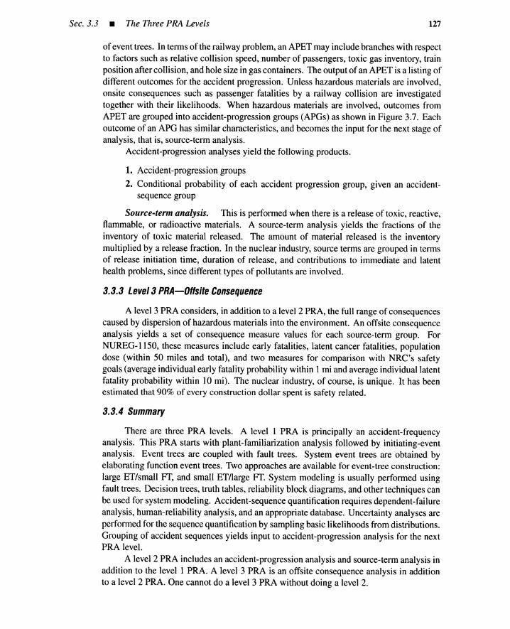
Sec. 3.3 • The Three PRA Levels 127
of event trees. In terms of the railway problem, an APET may include branches with respectto factors such as relative collision speed, number of passengers, toxic gas inventory, trainposition after collision, and hole size in gas containers. The output of an APET is a listing ofdifferent outcomes for the accident progression. Unless hazardous materials are involved,onsite consequences such as passenger fatalities by a railway collision are investigatedtogether with their likelihoods. When hazardous materials are involved, outcomes fromAPET are grouped into accident-progression groups (APGs) as shown in Figure 3.7. Eachoutcome of an APG has similar characteristics, and becomes the input for the next stage ofanalysis, that is, source-term analysis.
Accident-progression analyses yield the following products.
1. Accident-progression groups
2. Conditional probability of each accident progression group, given an accident-sequence group
Source-term analysis. This is performed when there is a release of toxic, reactive,flammable, or radioactive materials. A source-term analysis yields the fractions of theinventory of toxic material released. The amount of material released is the inventorymultiplied by a release fraction. In the nuclear industry, source terms are grouped in termsof release initiation time, duration of release, and contributions to immediate and latenthealth problems, since different types of pollutants are involved.
3.3.3 Leve/3 PRA-Offsite Consequence
A level 3 PRA considers, in addition to a level 2 PRA, the full range of consequencescaused by dispersion of hazardous materials into the environment. An offsite consequenceanalysis yields a set of consequence measure values for each source-term group. ForNUREG-1150, these measures include early fatalities, latent cancer fatalities, populationdose (within 50 miles and total), and two measures for comparison with NRC's safetygoals (average individual early fatality probability within 1 mi and average individual latentfatality probability within 10 mi). The nuclear industry, of course, is unique. It has beenestimated that 90% of every construction dollar spent is safety related.
3.3.4 Summary
There are three PRA levels. A level 1 PRA is principally an accident-frequencyanalysis. This PRA starts with plant-familiarization analysis followed by initiating-eventanalysis. Event trees are coupled with fault trees. System event trees are obtained byelaborating function event trees. Two approaches are available for event-tree construction:large ET/small Fl; and small ET/large Fr. System modeling is usually performed usingfault trees. Decision trees, truth tables, reliability block diagrams, and other techniques canbe used for system modeling. Accident-sequence quantification requires dependent-failureanalysis, human-reliability analysis, and an appropriate database. Uncertainty analyses areperformed for the sequence quantification by sampling basic likelihoods from distributions.Grouping of accident sequences yields input to accident-progression analysis for the nextPRA level.
A level 2 PRA includes an accident-progression analysis and source-term analysis inaddition to the level 1 PRA. A level 3 PRA is an offsite consequence analysis in additionto a level 2 PRA. One cannot do a level 3 PRA without doing a level 2.

128
3.4 RISK CALCULATIONS
3.4.1 The Level 3 PRA Risk Profile
Probabilistic Risk Assessment _ Chap. 3
The final result of a PRA is the risk profiles produced by assembling the results of allthree PRA risk-analysis studies.
Consequence measure. Consider a particular consequence measure denoted byCM divided into III small intervals I" l == I, ... , m.
Frequency andprobability. Define the following frequencies and conditional prob-abilities (see Figure 3.17):
1. !(IE/l): Annual frequency of initiating event h.
2. P(ASG; IIE/z): Conditional probability of accident-sequence group i, given oc-currence of initiating event h. This is obtained by an accident-frequency analysisusing accident-sequence event and fault trees.
3. P(APGj IASG;): Conditional probability of accident-progression group i. givenoccurrence of accident-sequence group i, This is obtained by accident-progressionanalysis using APETs.
4. P(STGkIAPGj ) : Conditional probability of source-term group k, given occur-rence of accident-progression group j. This is usually a zero-one probability.In other words, the matrix element for given values of j and k is 1.0 if APG j is
ACCident-FrequencyAnalysis
ASG;
Source-TermAnalysis
CM
Initiating-EventAnalysis
Accident-ProgressionAnalysis
P(CM 18TGk )
OffsiteConsequenceAnalysis
LegendsIE: Initiating EventASG: Accident Sequence Group
APG: Accident Progression GroupSTG: Source Term GroupeM: Consequence Measure Value
Figure 3.17. Frequency and conditional probabilities in PRA.
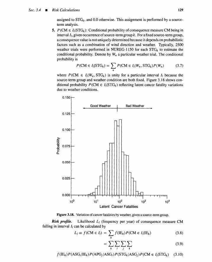
Sec.3.4 • Risk Calculations 129
assigned to STGk, and 0.0 otherwise. This assignment is performed by a source-term analysis.
5. P(CM E IIISTGk): Conditional probability of consequence measure CM being ininterval II, given occurrence of source-term group k, For a fixed source-term group,a consequence value is not uniquely determined because it depends on probabilisticfactors such as a combination of wind direction and weather. Typically, 2500weather trials were performed in NUREG-1150 for each STGk to estimate theconditional probability. Denote by Wn a particular weather trial. The conditionalprobability is
P(CM E It/STGk) == L P(CM E ItlWn , STGk)P(Wn ) (3.7)n
where P(CM E IIIWn , STGk) is unity for a particular interval I, because thesource-term group and weather condition are both fixed. Figure 3.18 shows con-ditional probability P(CM E I,ISTGk) reflecting latent cancer fatality variationsdue to weather conditions.
0.150
0.125
0.100
~
~:.0co 0.075.00'-a.
0.050
0.025
Good Weather Bad Weather
101 102 103
Latent Cancer Fatalities
o.000 t-----r---r--r-+...,..,...,."'Ti--".....A...-Ir-'--1'L......+-+-h..lr-T\-...........+-&-~_+_+....+n'-__,____y__~~
10°
Figure 3.18. Variation ofcancerfatalitiesby weather,givena source-term group.
Risk profile. Likelihood L, (frequency per year) of consequence measure CMfalling in interval II can be calculated by
L I == f(CM Ell) == L f(IEh)P(CM E I,IIEh) (3.8)h
== LLLL (3.9)h j k

130 Probabilistic Risk Assessment _ Chap. 3
A risk profile for consequence measure CM is obtained from pairs (L" I,), I ==I, ... ,111. A large number of risk profiles such as this are generated by uncertainty analysis.
Expected consequence. Denote by E(CMISTGk) a conditional expected value ofconsequence measure CM, given source-term group STGk. This value was calculated by a(weighted) sample mean of 2500 weather trials. An unconditional expected value E (CM)of consequence measure CM can be calculated by
E(CM) == LLLLh j k
f (IEh ) P(ASG; lIE,,)P(APGj IASG;) P(STGkIASGj ) E (CMISTGk )
3.4.2 The Level 2 PRA Risk Profile
(3.11 )
(3.12)
Release magnitude. Consider a level 2 PRA dealing with releases of a toxic ma-terial. Divide the release-magnitude range into small intervals I,. Denote by P(RM E
I,ISTGk) the conditional probability of release magnitude RM falling in interval I" givenoccurrence of source-term group k. This is a zero-one probability because each source-termgroup has a unique release magnitude.
Risk profile. Annual frequency L, of release magnitude RM falling in interval I, iscalculated in the same way as a consequence-measure likelihood. A risk profile for releasemagnitude RM is obtained from pairs (L" I,).
L, == f(RM E I,) == L L L L (3.13)" j k
Plant without hazardous materials. If hazardous materials are not involved, thena level 2 PRA only yields accident-progression groups; source-term analyses need notbe performed, Onsite consequences are calculated after accident-progression groups areidenti fied.
Consider, for instance, the single track passenger railway problem in Section 3.1.2.Divide a fatality range into small intervals I,. Each interval represents a subrange of fa-talities, NF. Denote by P(NF E I,IAPGj ) the conditional probability of the number offatalities falling in interval I" given occurrence of accident-progression group j. Thisis a zero-one probability where each accident-progression group uniquely determines thenumber of fatalities. Annual frequency L, of fatality interval I, is calculated as
L, == f(NF E I,) == LLL" j
A risk profile for the number of fatalities NF is obtained from pairs (L" I,).
3.4.3 The Leve/1 PRA Risk Profile
(3.15)
(3.16)
A level I PRA deals mainly with accident frequencies; for instance, the annual fre-quency of railway collisions. Denote by peA IASG;) the conditional probability of accidentA, given occurrence of accident-sequence group i . This is a zero-one probability. Annual

Sec. 3.4 • Risk Calculations
frequency L of accident A is given by
L == f(A) == L L f(IEh)P(ASG; \IEh)P(A\ASG;)h
3.4.4 Uncertainty ofRisk Profiles
131
(3.17)
Likelihood samples. The accident-frequency analyses, accident-progression anal-yses, and source-term analyses are performed several hundred times (200 in NUREG-1150) by sampling frequencies and probabilities from failure data distributions. Thisyields several hundred combinations of the three analyses. Each sample or observationuniquely determines initiating-event frequency f (IEh) , accident-sequence-group probabil-ity P(ASG; \IEh) , accident-progression-group probability P(APGj \ASG;), source-term-group probability P(STGkIASGj ) , and consequence probability P(CM E IllSTGk).
Uncertainty as distributions. Each observation yields a unique risk profile for aconsequence measure, and several hundred risk profiles are obtained by random sampling.Distribution patterns of these risk profiles indicate uncertainty in the risk profile. Figure3.19 shows a 95% upper bound, 5% lower bound, mean, and median risk profiles on a logarithmetic scale.
10-3"-ctSQ)
10-4>;-"- 95%00 10-5 MeanctSQ)
a:10-6
Median..........>- 5%UCQ) 10-7:::J0-Q)"-
10-8u..tI)tI)Q)
10-9ox
W10-10
100 101 102 103 104 105
Latent Cancer Fatalities
Figure 3.19. Distribution of latent cancer fatality risk profiles.
Samples of expected consequence E(CM) of consequence measure CM are obtainedin a similar way. If conditional expected values E(CM\STGk) obtained from weathertrials are used for a fixed source-term group, repetition of time-consuming consequencecalculations are avoided as long as an observation yields the source-term group. Variationsof expected consequence E(CM) are depicted in Figure 3.20, which includes 95% upperbound, 5% lower bound, median and mean values.
3.4.5 Summary
Risk profiles are calculated in three PRA levels by using conditional probabilities.Level 3 risk profiles refer to consequence measures, level 2 profiles to release magnitudes,and level 1 profiles to accident occurrence. Uncertainties in risk profiles are quantified interms of profile distributions.
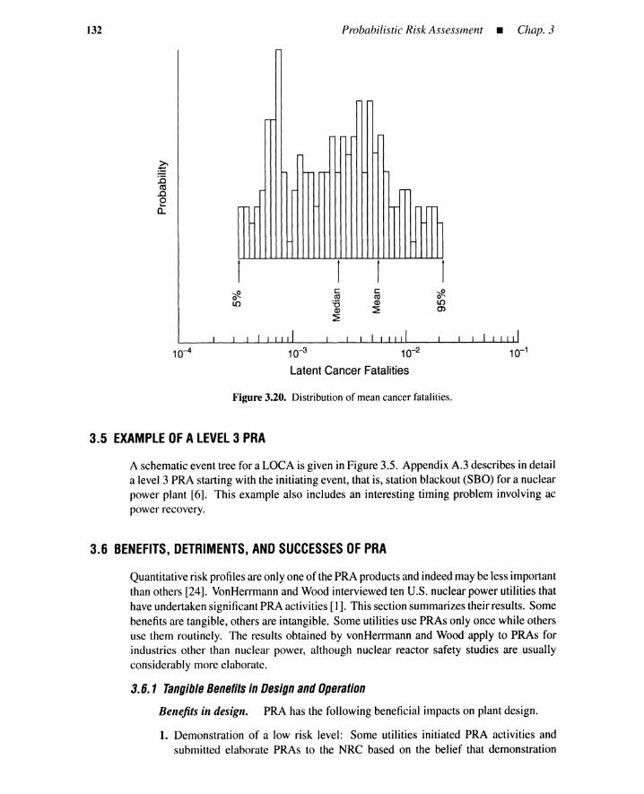
132
;:RoLO
Probabilistic Risk Assessment _ Chap. 3
;:RoLOen
10-3 10-2
Latent Cancer Fatalities
Figure 3.20. Distribution of mean cancer fatalities.
3.5 EXAMPLE OF A LEVEL 3 PRA
A schematicevent tree for a LOCA is given in Figure 3.5. AppendixA.3 describes in detaila level 3 PRA starting with the initiatingevent, that is, station blackout (SBO) for a nuclearpower plant [6]. This example also includes an interesting timing problem involving acpower recovery.
3.6 BENEFITS, DETRIMENTS, AND SUCCESSES OF PRA
Quantitativeriskprofilesare onlyone of the PRA productsand indeedmaybe less importantthan others [24]. VonHerrmann and Wood interviewedten U.S. nuclear power utilities thathave undertakensignificantPRA activities [I]. This sectionsummarizestheir results. Somebenefitsare tangible, others are intangible. Some utilities use PRAs only once while othersuse them routinely. The results obtained by vonHerrmann and Wood apply to PRAs forindustries other than nuclear power, although nuclear reactor safety studies are usuallyconsiderably more elaborate.
3.6.1 Tangible Benefits in Design and Operation
Benefits in design. PRA has the following beneficial impacts on plant design.
1. Demonstration of a low risk level: Some utilities initiated PRA activities andsubmitted elaborate PRAs to the NRC based on the belief that demonstration
Sec. 3.6 • Benefits, Detriments, and SuccessesofPRA 133
of a low level of risk from their plants would significantly speed their licensingprocess. (They were wrong. Regulatory malaise, public hearings, and lawsuitsare the major delay factors in licensing.)
2. Identification of hitherto unrecognized deficiencies in design.
3. Identification of cost-beneficial design alternatives. Some utilities routinely usePRAs to evaluate the cost and safety impact of proposed plant modifications. PRAscan be useful in industry-regulatory agency jousts:(a) To obtain exemption from an NRC proposed modification that would not
improve safety in a cost-beneficial manner.(b) Replacement of an NRC proposed modification with a significantly more
cost-beneficial modification.
Benefits in operation. This includes improvements in procedures and control.
1. Improved procedures: Some utilities identified specific improvements in mainte-nance, testing, and emergency procedures that have a higher safety impact thanhardware modifications. These utilities have successfully replaced an expensiveNRC hardware requirement with more cost-effective procedure upgrades.
2. Improved control: One utility was able to demonstrate that additional water-levelmeasuring would not enhance safety, and that the addition of another senior reactoroperator in the control room had no safety benefit.
3.6.2 Intangible Benefits
Staffcapabilities. PRA brings the following staff-capability benefits.
1. Improved plant knowledge: Engineering and operations personnel, when exposedto the integrated perspective of a PRA, are better able to understand overall plantdesign and operation, especially the interdependencies between and among sys-tems.
2. Improved operator training: Incorporation of PRA models and results in operatortraining programs has significantly enhanced ability to diagnose and respond toincidents.
Benefits in NRC interaction. PRA yields the following benefits in interactions withthe NRC.
1. Protection from NRC-sponsored studies: One utility performed their own studyto convince the NRC not to make their plant the subject of an NRC study. Theutility believes that:(a) NRC-sponsored studies, because they are performed by outside personnel
who may have insufficient understanding of the plant-specific features, mightidentify false issues or problems or provide the NRC with inaccurate infor-mation.
(b) The utility could much more effectively interact with the NRC in an intelligentmanner concerning risk issues if they performed their own investigation.
(c) Even where valid issues were identified by NRC-sponsored studies, the rec-ommended modifications to address these issues were perceived to be bothineffective and excessively costly.
134 Probabilistic Risk Assessment _ Chap. 3
2. Enhanced credibility with the NRC: Some utilities strongly believe that their PRAactivities haveallowed them to establish or enhance their reputation with the NRC,thus leading to a significantly improved regulatory process. The NRC now hasa higher degree of faith that the utility is actively taking responsibility for safeoperation of their plant.
3. Efficient response to the NRC: PRAs allow utilities to more efficiently and effec-tively respond to NRC questions and concerns.
3.6.3 PRA Negatives
Utilities cited potential negatives in the following areas. The first two can be resolvedby PRAs, although the resources expended in clearing up the issues could be excessive.
1. Identification of problems of little safety importance: A few utilities cited thedanger that, if PRAs were submitted to the NRC, NRC staff would inappropriatelyuse the study to magnify minor safety problems. The utilities stated that PRAprovided them with the means to identify effective resolutions to these problemsbut resources to clear up the issues were excessive and unwarranted.
For example, in response to a PRA submittal that focused on a problem,the NRC initiated inquiries into the adequacy of a plant's auxiliary feedwatersystem (AFWS) reliability. The AFWS was modeled in a conservative mannerin the submission. The NRC took the AFWS reliability estimate out of contextand required the utility to divert resources to convince the NRC that no problemsactually existed with the AFWS.
2. Familiarization with the study: The utilities must ensure that the individuals whointeract with the NRC are familiar with the PRA study. Failure to do this can pro-duce modest negative impacts on the utility-regulator relationship. The questionof whether a utility should send lawyers and/or engineers to deal with the NRC isdiscussed in Chapter 12.
Although the major focus in Section 3.6 has been on the nuclear field, NRC-typeprocedures and policies are being adopted by the EPA,FDA, and state air and water qualityagencies, whose budgets have more than quadrupled over the last twenty years (whilemanufacturing employment has dropped 15%).
3.6.4 Success Factors ofPRA Program
3.6.4.1 Three PRA levels. The PRA successescan bedefined in terms of the abilityto complete the PRA, ability to derive significantbenefits from a PRA after it is completed,and ability to produce additionalanalyses withoutdependence on outsidecontractor support.
The majority of level 3 PRAs were motivated by the belief that the nuclear reactorlicensing process would be appreciably enhanced by submittal of a PRA that demonstrateda low level of risk. No utility performed a full level 2 PRA to evaluate source terms. Thisindicates that utilities believe that the logical end points of a PRA are either an assessmentof core damage frequency (level I) or public health consequences (level 3).
PRA programs, whoseprimary motivationis to prioritize plant modificationactivities,deal with level I PRAs. It is generally believedthat a level 1PRA providesan adequate basisfor evaluating, comparing, and prioritizing proposed changes to plant design and operation.
Sec. 3.6 • Benefits, Detriments, and SuccessesofPRA
3.6.4.2 Staffing requirements
135
In-house versuscontractorstaff. All of the utilities used considerable contract sup-port in their initial studies and all indicated that this was important in getting their programsstarted in an efficient and successful manner. However, a strong corporate participation inthe development process is a necessary condition for success.
Attributes ofan in-house PRA team. Utilities that have assigned personnel withthe following characteristics to their PRA team report benefits from their PRA expenditures.
1. Possess detailed knowledge of plant design and dynamic behavior. Experiencedplant personnel have a more detailed knowledge of plant design and operation thancontractors.
2. Be known and respected by managers and decision makers throughout the orga-nization.
3. Have easy access to experienced personnel.
4. Possess the ability to communicate PRA insights and results in terms familiar todesigners, operators, and licensing personnel.
5. Understand the PRA perspective and be inclined toward investigative studies.
On the other hand, utilities that have assigned personnel who are disconnected fromother members of the utility staff in design, operations, and licensing and are unable toeffectively or credibly interact with other groups have experienced the least benefits fromtheir PRAs, regardless of the PRA training or skills of these individuals.
Roles ofin-house staff. Successful programs have used either of the following twoapproaches.
1. Use of company personnel in a detailed technical review role. This takes advantageof their plant-specific knowledge and their access to knowledgeable engineers andoperators. It also provides an effective mechanism for them to learn the details ofthe models and how they are consolidated into an overall risk model.
2. An evolutionary technology transfer process in which the utility personnel re-ceive initial training, and then perform increasingly responsible roles as the tasksprogress and as their demonstrated capabilities increase.
3.6.4.3 Technical tools and methods
Details ofmodels. Detailed plant models were essential because
1. these models were required for identifying unrecognized deficiencies in designand operation, and for identifying effective alternatives
2. the models created confidence outside the PRA group
Computer software. Utilities interviewed developed large, detailed fault-tree mod-els and used mainframe computer codes such as SETS or WAM to generate cut sets andquantify the accident sequences. Most utilities warned against overreliance on "intelli-gent" software; the computer software plus a fundamental understanding of the models byexperienced engineers are necessary.

136 Probabilistic Risk Assessment _ Chap. 3
Methodology. There are methodological options such as large versus small eventtrees, fault trees versus block diagrams, or SETS or WAM. The PRA successes are lessdependent on these methodological options.
Documentation. Clear documentation of the system models is essential. It is alsoimportant to provide PRA models, results, and insights written expressly for non-technicalgroups to present this information in familiar terms.
3.6.4.4 Visible senior management advocacy. This produces the following bene-fits.
1. Continued program funding
2. Availability of quality personnel
3. Evaluation of PRA potential in an unbiased manner by other groups
4. An increased morale and commitment of the PRA team to make the PRA producethe benefitsexpected by upper management
5. An increased commitment to modify the plant design and operation, even if thecost is significant, if the PRA analysis identifies such a need, and documents itscost-effectiveness
3.6.5 Summary
PRA providestangiblebenefitsin improvedplantdesignand operation,and intangiblebenefitsin strengtheningstaffcapabilityand interactionwithregulatoryagencies. PRA alsohas some detriments. Factors for a successful PRA are presented from points of view ofin-house versus contractor staff, attributes of in-house PRA teams, roles of in-house staff,depth of modeling detail, computer software, methodology and documentation, and seniormanagement advocacy.
REFERENCES[I] vonl-lerrmann, J. L., and P.J. Wood. "The practical applicationofPRA: An evaluation
of utility experience and USNRC perspectives," Reliability Engineering and SystemSafety, vol. 24, no. 2, pp. 167-198, 1989.
[2] Papazoglou, I. A., O. Aneziris, M. Christou, and Z. Nivoliantou. "Probabilistic safetyanalysis of an ammonia storage plant." In Probabilistic Safety Assessment and Man-agement, edited by G. Apostolakis, pp. 233-238. New York: Elsevier, 1991.
[3] USNRC. "Reactor safety study: An assessment of accident risk in U.S. commercialnuclear power plants." USNRC, WASH-1400, NUREG-75/014, 1975.
[4] IAEA. "Computer codes for level 1 probabilistic safety assessment." IAEA, IAEA-TECDOC-553, June 1990.
[5] Apostolakis, G. E., J. H. Bickel, and S. Kaplan. "Editorial: Probabilistic risk assess-ment in the nuclear powerutility industry," Reliability Engineering and System Safety,vol. 24, no. 2,pp.91-94, 1989.
[6] USNRC. "Severe accident risks: An assessment for five U.S. nuclear power plants."USNRC, NUREG-1150, vol. 2, 1990.
[7] USNRC. "PRA procedures guide: A guide to the performance of probabilistic riskassessments for nuclear power plants." USNRC, NUREGICR-2300, 1983.
Chap. 3 • References 137
[8] Holloway, N. J. "A method for pilot risk studies." In Implications ofProbabilistic RiskAssessment, edited by M. C. Cullingford, S. M. Shah, and J. H. Gittus, pp. 125-140.New York: Elsevier Applied Science, 1987.
[9] Lambert, H. E. "Fault tree in decision making in systems analysis." Lawrence Liver-
more Laboratory, UCRL-51829, 1975.
[10] Department of Defense. "Procedures for performing a failure mode, effects and criti-cality analysis." Department of Defense, MIL-STD-1629A.
[11] Taylor, R. RISfj> National Laboratory, Roskilde, Denmark. Private Communication.
[12] Villemeur, A. Reliability, Availability, Maintainability and Safety Assessment, vol. 1and 2. New York: John Wiley & Sons, 1992.
[13] Mckinney, B. T. "FMECA, the right way." In Proc. Annual Reliability and Maintain-ability Symposium, pp. 253-259,1991.
[14] Hammer, W. Handbook ofSystem and Product Safety. Englewood Cliffs, NJ: Prentice-
Hall, 1972.
[15] Lawley, H. G. "Operability studies and hazard analysis," Chemical EngineeringProgress, vol. 70, no. 4, pp. 45-56, 1974.
[16] Roach, J. R., and F. P. Lees. "Some features of and activities in hazard and operability(Hazop) studies," The Chemical Engineer, pp. 456-462, October, 1981.
[17] Kletz, T. A. "Eliminating potential process hazards," Chemical Engineering, pp. 48-68, April 1, 1985.
[18] Suokas, J. "Hazard and operability study (HAZOP)." In Quality Management ofSafetyand Risk Analysis, edited by J. Suokas and V. Rouhiainen, pp. 84-91. New York:
Elsevier, 1993.
[19] Venkatasubramanian, V., and R. Vaidhyanathan. "A knowledge-based framework forautomating HAZOP analysis," AIChE Journal, vol. 40, no. 3, pp. 496-505, 1994.
[20] Russomanno, D. J., R. D. Bonnell, and J. B. Bowles. "Functional reasoning in a failuremodes and effects analysis (FMEA) expert system." In Proc. Annual Reliability andMaintainability Symposium, pp. 339-347, 1993.
[21] Hake, T. M., and D. W. Whitehead. "Initiating event analysis for a BWR low powerand shutdown accident frequency analysis." In Probabilistic Safety Assessment andManagement, edited by G. Apostolakis, pp. 1251-1256. New York: Elsevier, 1991.
[22] Arrieta, L. A., and L. Lederman. "Angra I probabilistic safety study." In ImplicationsofProbabilistic Risk Assessment, edited by M. C. Cullingford, S. M. Shah, and J. H.Gittus, pp. 45-63. New York: Elsevier Applied Science, 1987.
[23] Swain, A. D. "Accident sequence evaluation program: Human reliability analysisprocedure." Sandia National Laboratories, NUREGICR-4722, SAND86-1996, 1987.
[24] Konstantinov, L. V. "Probabilistic safety assessment in nuclear safety: Internationaldevelopments." In Implications of Probabilistic Risk Assessment, edited by M. C.Cullingford, S. M. Shah, and J. H. Gittus, pp. 3-25. New York: Elsevier AppliedScience, 1987.
[25] Ericson, D. M., Jr., et al. "Analysis of core damage frequency: Internal events method-ology." Sandia National Laboratories, NUREGICR-4550, vol. 1, Rev. 1, SAND86-2084,1990.
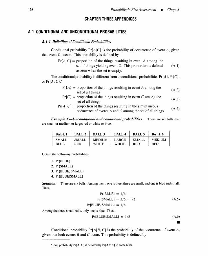
138 Probabilistic Risk Assessment _ Chap. 3
CHAPTER THREE APPENDICES
A.1 CONDITIONAL AND UNCONDITIONAL PROBABILITIES
A.1.1 Definition ofConditional Probabilities
(A.I)
(A.4)
(A.3)
(A.2)
Conditional probability Pr{AIC} is the probability of OCCUITence of event A, giventhat event C occurs. This probability is defined by
Pr{A IC} == proportion of the things resulting in event A among theset of things yielding event C. This proportion is definedas zero when the set is empty.
The conditional probability isdifferent from unconditionalprobabilitiesPr{A}, Pr{C},or Pr{A, C}:*
Pr{ A} == proportion of the things resulting in event A among theset of all things
Pr{C} == proportion of the things resulting in event C among theset of all things
Pr{A, C} == proportion of the things resulting in the simultaneousoccurrence of events A and C among the set of all things
Example A-Unconditional and conditional probabilities. There are six balls thatare small or medium or large; red or white or blue.
BALL 1 BALL 2 BALL 3 BALL 4 BALLS BALL 6
SMALLBLUE
SMALLRED
MEDIUMWHITE
LARGEWHITE
SMALLRED
MEDIUMRED
Obtain the following probabilities.
1. Pr{BLUE}
2. Pr{SMALL}
3. Pr{BLUE,SMALL}
4. Pr{BLUEISMALL}
Solution: There are six balls. Among them, one is blue, three are small, and one is blue and small.Thus,
Pr{BLUE} = 1/6
Pr{SMALL} = 3/6 = 1/2
Pr{BLUE,SMALL} = 1/6
Among the three small balls, only one is blue. Thus,
Pr{BLUEISMALL} = 1/3
(A.5)
(A.6)
•Conditional probability Pr{A IB, C} is the probability of the occurrence of event A,
given that both events Band C occur. This probability is defined by
*Joint probability Pr{A, C} is denoted by Pr{A n C} in some texts.

AppendixA.I • Conditional and Unconditional Probabilities 139
Pr{A \B, C} == proportion of the things yielding event A among theset of things resulting in the simultaneous (A.7)occurrence of events Band C
Example B-Conditional probability. Obtain
1. Pr{BALL 2}
2. Pr{SMALL, RED}
3. Pr{BALL 2, SMALL,RED}
4. Pr{BALL 2\SMALL,RED}
5. Pr{BALL IISMALL,RED}
Solution: Amongthe six balls, two are smalland red, and one is at the same time ball 2, smallandred. Thus,
Pr{BALL 2} = 1/6
Pr{SMALL, RED} = 2/6 = 1/3
Pr{BALL 2, SMALL,RED} = 1/6
Ball 2 is one of the two small red balls; therefore
Pr{BALL 2\SMALL,RED} = 1/2
Ball I does not belong to the set of the two small red balls. Thus
Pr{BALL IISMALL,RED} = 0/2 = 0
A.1.2 Chain Rule
(A.8)
(A.9)
(A.IO)
•The simultaneous existence of events A and C is equivalent to the existence of event
C plus the existence of event A under the occurrence of event C. Symbolically,
(A, C) ¢} C and (AIC)
This equivalence can be extended to probabilities:
Pr{A, C} == Pr{C}Pr{AIC}
(A.I I)
(A.12)
More generally,
Pr{A 1, A2 , ••. , An} == Pr{A I }Pr{A2IA I } ••• Pr{AnIA I , A2 , ••. , An-I} (A.I3)
If we think of the world (the entire population) as having a certain property W, then equation(A.I2) becomes:
Pr{A, C\W} == Pr{C\W}Pr{A\C, W} (A.I4)
These equations are the chain rule relationships. They are useful for calculating si-multaneous (unconditional) probabilities from conditional probabilities. Some conditionalprobabilities can be calculated more easily than unconditional probabilities, because con-ditions narrow the world under consideration.
Example C-Chain rule. Confirmthe chain rules:
1. Pr{BLUE, SMALL} = Pr{SMALL}Pr{BLUE\SMALL}
2. Pr{BALL 2, SMALL\RED} = Pr{SMALL\RED}Pr{BALL 2\SMALL,RED}

140 Probabilistic Risk Assessment _ Chap. 3
Solution: From Example A
Pr{BLUE,SMALL} = 1/6
Pr{SMALL} = 1/2
Pr{BLUEISMALL} = 1/3
The first chain rule is confirmed, because
1/6 = (1/2)(1/3)
(A. IS)
(A.16)
Among the three red balls, two are small, and one is at the same time small and ball 2. Thus
Pr{BALL2, SMALLIRED} = 1/3
Pr{SMALLIRED} = 2/3
Only one ball is ball 2 among the two small red balls.
Pr{BALL2ISMALL, RED} == 1/2
Thus the second chain rule is confirmed, because1
"3 = (2/3)(1/2)
A.1.3 Alternative Expression ofConditional Probabilities
(A.17)
(A.18)
(A.19)
•From the chain rule of equations (A.12) and (A.14), we have
Pr{AIC} = Pr{A, C} (A.20)Pr{C}
Pr{AIC W} = Pr{A, C1W} (A.21), Pr{CIW}
We see that the conditional probability is the ratio of the unconditional simultaneous prob-ability to the probability of condition C.
Example D-Conditional probability expression. Confirm:
1. Pr{BLUEISMALL} = Pr{BLUE,SMALL}/Pr{SMALLl
2. Pr{BALL2ISMALL, RED} = Pr{BALL 2, SMALLIREDI/Pr{SMALLIREDl
Solution: From Example C
1/3 == ~ == 1/3, for the first equation1/2
1/2 = ~j~ = 1/2, for the second equation
A.1.4 Independence
Event A is independent of event C if and only if
Pr{AIC} == Pr{A}
(A.22)
•
(A.23)
This means that the probability of event A is unchanged by the occurrence of event C.Equations (A.20) and (A.23) give
Pr{A, C} == Pr{A }Pr{C} (A.24)
This is another expression for independence. Wesee that if event A is independent of eventC, then event C is also independent of event A.
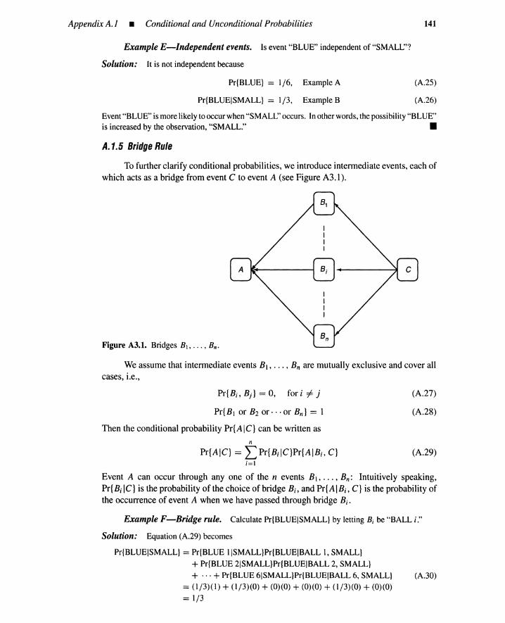
Appendix A.J • Conditional and Unconditional Probabilities
Example E-Independent events. Is event "BLUE" independent of "SMALL"?
Solution: It is not independent because
Pr{BLUE} = 1/6, Example A
Pr{BLUEISMALL} = 1/3, Example B
141
(A.25)
(A.26)
Event "BLUE" is more likely to occur when "SMALL" occurs. In other words, the possibility "BLUE"is increased by the observation, "SMALL." •
A.1.5 Bridge Rule
To further clarify conditional probabilities, we introduce intermediate events, each ofwhich acts as a bridge from event C to event A (see Figure A3.1).
Figure A3.1. Bridges B1, ••• , Bn•
We assume that intermediate events B1, ••• , B; are mutually exclusive and cover allcases, i.e.,
Pr{B;, Bj } = 0, for i i= j
Pr{B1 or B2 or·· -or Bn } = 1
Then the conditional probability Pr{AIC} can be written as
n
Pr{AIC} == LPr{B;\C}Pr{AIB;, C};=1
(A.27)
(A.28)
(A.29)
Event A can occur through anyone of the n events B1, ... , Bn : Intuitively speaking,Pr{B; IC} is the probability of the choice of bridge B;, and Pr{AIB;, C} is the probability ofthe occurrence of event A when we have passed through bridge B;.
Example F-Bridge rule. Calculate Pr{BLUEISMALL} by letting B; be "BALL i."
Solution: Equation (A.29) becomes
Pr{BLUEISMALL} = Pr{BLUE IISMALL}Pr{BLUEIBALL 1, SMALL}
+ Pr{BLUE 2ISMALL}Pr{BLUEIBALL 2, SMALL}
+ ... + Pr{BLUE 6ISMALL}Pr{BLUEIBALL 6, SMALL} (A.30)
= (1/3)(1) + (1/3)(0) + (0)(0) + (0)(0) + (1/3)(0) + (0)(0)
= 1/3
142 Probabilistic Risk Assessment _ Chap. 3
When there is no ball satisfying thecondition, the correspondingconditionalprobabilityis zero. Thus
Pr{BLUEIBALL 3, SMALL} == 0
Equation (A.30) confirms the result of Example A.
A.1.6 Bayes Theorem forDiscrete Variables
Bayes theorem, in a modified and useful form, may be stated as:
Posterior probabilities ex prior probabilities x likelihoods
(A.31)
•
(A.32)
where the symbol ex means "are proportional to." This relation may be formulated in ageneral form as follows: if
1. the Ai'S are a set of mutually exclusive and exhaustive events, for i == 1, ... , n;
2. Pr{A i} is the prior (or a priori) probability of Ai before observation;
3. B is the observation; and
4. Pr{B IAi} is the likelihood, that is, the probability of the observation, given that Aiis true, then
Pr{A i, B} Pr{A i }Pr{BIAi}Pr{A;IB} == == -----
Pr{B} L;Pr{A;}Pr{BIA;}(A.33)
where Pr{A; IB} is the posterior (or a posteriori) probability, meaning the proba-bility of A; now that B is known. Note that the denominator of equation (A.33) issimply a normalizing constant for Pr{A; IB}, ensuring L Pr{A; IB} == 1.
The transformation from Pr{A;} to Pr{A;I B} is called the Bayes's transform, Itutilizes the fact that the likelihood of Pr{BIA;} is more easily calculated than Pr{A; IB}.If we think of probability as a degree of belief, then our prior belief is changed, by theevidence observed, to a posterior degree of belief.
Example G-Bayes theorem. A randomly sampled ball turns out to be small. Use Bayestheorem to obtain the posterior probability that the ball is ball 1.
Solution: From Bayes theorem
Pr{SMALLIBALL 1}Pr{BALL I}Pr{BALL IISMALL} = -6-----------
Li=l Pr{SMALLIBALL i}Pr{BALL i}(A.34)
Because the ball is sampled randomly, we have prior probabilities before the small ball observation:
Pr{BALL i} = 1/6, i == 1, ... ,6
From the ball data of Example A, likelihoods of small ball observationare
(A.35)
{I ,
Pr{SMALLIBALL i} =0,
Thus the Bayes formula is calculated as
i = 1,2,5,
i == 3,4,6(A.36)
Pr BALL 1 SMALL = 1 x (1/6) = ~{ I } (I + 1+0+0+ 1 +0)(1/6) 3
This is consistent with the fact that ball 1 and two other balls are small.
(A.37)
•

Appendix A.2 • Venn Diagrams and Boolean Operations
A.1.7 Bayes Theorem forContinuous Variables
Let
143
(A.38)
1. x = the continuous valued parameter to be estimated;
2. p{x} = the prior probability density of x before observation;"
3. Y = (Yl, ... , YN): N observations of an attribute of x;
4. P{y[x] = likelihood, that is, the probability density of the observations given thatx is true; and
5. p{x IY} = the posterior probability density of x.
From the definition of conditional probabilities,
p{xIY} = p{x,y} = p{x,y}p{y} f [numerator]dx
The numerator can be rewritten as
p{x,y} = p{x}p{Ylx}
yielding Bayes theorem for the continuous valued parameter x.
p{x Lv} = p{x} pfylx}f [numerator]dx
Bayes theorem for continuous x and discrete B is
p{xIB} = p{x}Pr{Blx}f [numerator]dx
For discrete Ai and continuous y
{ }Pr{Ai }p{YIA i}
Pr Ai IY = -----Li [numerator]
A.2 VENN DIAGRAMS AND BOOLEAN OPERATIONS
A.2.1 Introduction
(A.39)
(A.40)
(A.41)
(A.42)
In Venndiagrams the set of all possible causes is denoted by rectangles, and a rectanglebecomes a universal set. Some causes in the rectangle result in an event but others do not.Because the event occurrence is equivalent to the occurrence of its causes, the event isrepresented by a closed region-that is, a subset-within the rectangle.
Example H-Venn diagram expression. Assumean experimentwhere we throwa diceand observe its outcome as a cause of events. Consider the events A, B, and C, which are definedas
A = {outcome = 3, 4, 6}
B = {3~ outcome .s 5}
C = {3~ outcome ~ 4}
Represent these events by a Venndiagram.
*Denote by X a continuous random variable having probability density p{x}. Quantity pIx }dx is theprobabilitythat randomvariableX has a value in a small interval (x, x + dx).
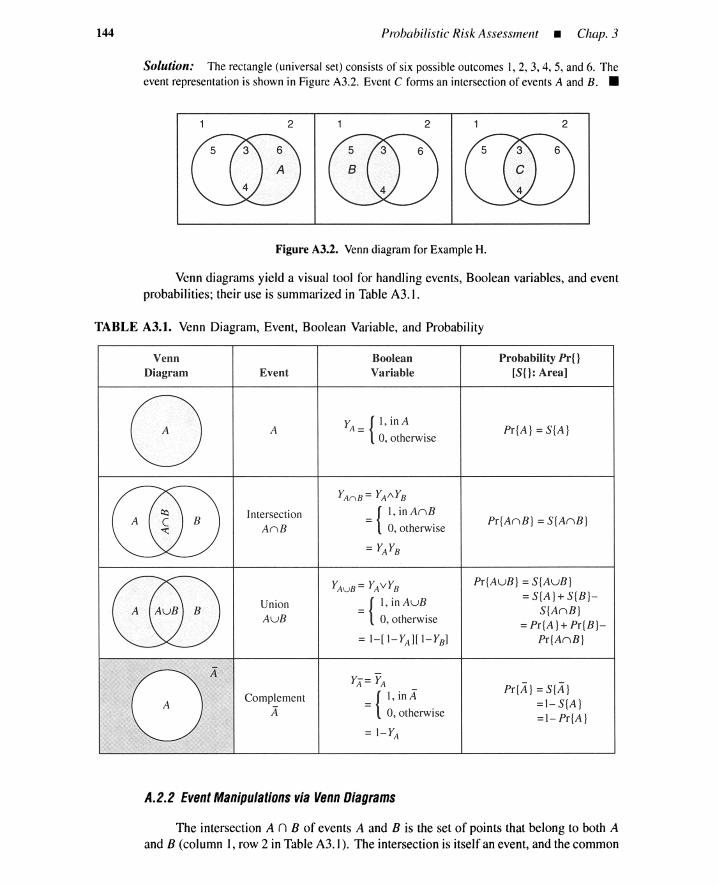
144 Probabilistic Risk Assessment • Chap. 3
Solution: The rectangle (universal set) consists of six possible outcomes 1,2,3,4,5, and 6. Theevent representation is shown in Figure A3.2. Event C forms an intersectionof events A and B. •
2 2 2
FigureA3.2. Venn diagram for Example H.
Venn diagrams yield a visual tool for handling events, Boolean variables, and eventprobabilities; their use is summarized in Table A3.1.
TABLE A3.1. Venn Diagram, Event, Boolean Variable, and Probability
VennDiagram
oEvent
A
IntersectionAnB
UnionAuB
ComplementA
BooleanVariable
Y {I , in AA=0, otherwise
YAn B = YAI\ YB
{I , in AnB
= 0, otherwise
=YAYB
Yx = YA
{I , inA
= 0, otherwise
= I- YA
Probability Pr(}
[SO: Area]
Pr( A} =SIA l
Pr {AnB} = S{AnB}
Pr {AuB} =StAuB }= S{A }+S{B}-
S{AnB }=Pr{ A} + Pr{B}-
Pr{ AnB}
Pr{A} =S{A}= I-S{A}=1-Pr{A}
A.2.2 Event Manipulations via Venn Diagrams
The intersection A n B of events A and B is the set of points that belong to both Aand B (column I, row 2 in Table A3.1). The intersection is itself an event, and the common
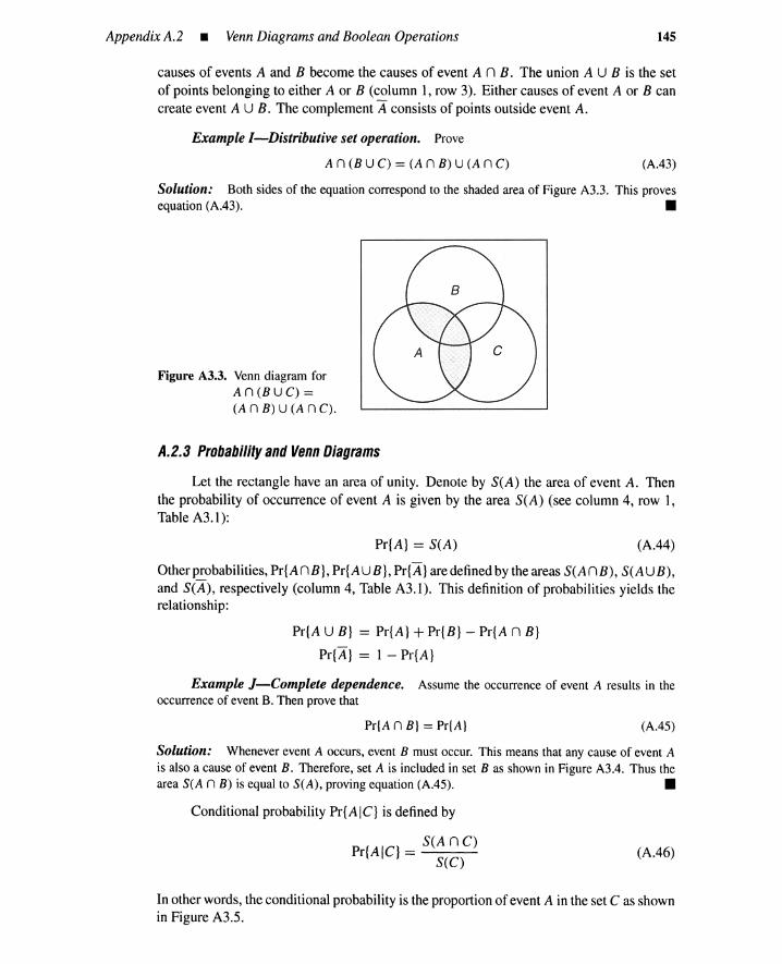
AppendixA.2 • Venn Diagrams and BooleanOperations 145
causes of events A and B become the causes of event A n B. The union A U B is the setof points belonging to either A or B (column I, row 3). Either causes of event A or B cancreate event AU B. The complement A consists of points outside event A.
Example I-Distributive set operation. Prove
An (B U C) = (An B) U (A n C) (A.43)
Solution: Both sides of the equation correspond to the shaded areaof Figure A3.3. This provesequation (A.43). •
Figure A3.3. Venn diagram forAn (B U C) =(A n B) U (A n C).
A.2.3 Probability and Venn Diagrams
Let the rectangle have an area of unity. Denote by SeA) the area of event A. Thenthe probability of occurrence of event A is given by the area SeA) (see column 4, row I,Table A3.1):
Pr{A} = S(A) (A.44)
Other probabilities, Pr{AnB}, Pr{AUB}, Pr{A} are defined by the areas S(AnB), S(AUB),and S(A), respectively (column 4, Table A3.1). This definition of probabilities yields therelationship:
Pr{A U B} = Pr{A) + Pr{B} - Pr{An B)
Pr{A} = I - Pr{A}
Example J-Complete dependence. Assume the occurrence of event A results in theoccurrence of event B. Thenprove that
Pr{A n B} = Pr{A} (A.45)
Solution: Whenever event A occurs, event B must occur. This means that any cause of event Ais also a cause of event B. Therefore, set A is included in set B as shown in Figure A3.4. Thus theareaS(A n B) is equal to S(A), proving equation (A.45). •
Conditional probability Pr{AIC} is defined by
Pr{AIC} = SeA n C)S(C)
(A.46)
In other words, the conditional probability is the proportion of event A in the set C as shownin Figure A3.5.
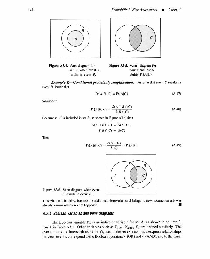
146
Figure A3.4. Venn diagram forA n B when event Aresults in event B.
Probabilistic Risk Assessment • Chap . 3
Figure A3.5. Venn diagram forconditional prob-ability Pr(AIC}.
Example K-Conditional probability simplification. Assume that event C results inevent B. Prove that
Pr(AIB. C}= Pr(AIC} (A.47)
Solution:
SeA n B n C)Pr(A IB. C } = S(B n C)
Because set C is included in set B, as shown in Figure A3.6, then
SeA n B n C) = SeA n C)
S(B n C) = S(C)
Thus
SeA n C)Pr(AIB . C} = = Pr(AIC}
S(C )
(A.48)
(A.49)
Figure A3.6. Venn diagram when eventC results in event B.
This relation is intuitive, because the additional observation of B brings no new information as it wasalready known when event C happened. •
A.2.4 Boolean Variables and Venn Diagrams
The Boolean variable YA is an indicator variable for set A, as shown in co lumn 3,row I in Table A3.1. Other variables such as YAUB, YAnB, YA are defined similarly. Theevent unions and intersections, U and n, used in the set expressions to express relat ionshipsbetwee n events, correspond to the Boolean operators v (OR) and 1\ (AND), and to the usual

AppendixA.2 • Venn Diagramsand Boolean Operations 147
algebraic operations - and x as shown in Table A3.2. Probability equivalences are alsoin Table A3.2; note that Pr{B;} = E{Y;} ; thus for zero-one variable Y;, EO is an expectednumber, or probability. Variables YAUB, YAnB, and YA are equal to YA V YB, YA /\ YB, and
YA, respectively .
TABLE A3.2. Event , Boolean, and Algebraic Operations
Event Boolean Algebraic Note
Bi Yi = 1 Yi = I Event i exists
B; Y; =0 Yi =0 Event i does not existB; n s, Y; /\Yj=1 Y;Yj = 1 Pr{B; n Bj} = E{Y; /\ Yj}B; U e, Y; vYj=1 I - [I - Y;)[I - Yj] = I Pr{B; U Bj) = E{Y; v Yj)B1 n ···n e, Y, /\ ... /\ Yn = 1 YI X • •• X Yn = I Pr{B I n .. ·n Bn)
= E{Y! /\ .. . /\ Ynln
B, U·· · U e, Y, v ·· · V Yn = I 1- TI[I - Y;l = I Pr{BI U · · · U Bn);=1 = E(YI V . .. V Yn)
Addition (+) and product (.) symbols are often used as Boolean operation symbolsv and r-; respectively, when there is no confusion with ordinary algebraic operations; theBoolean product symbol is often omitted.
YA V YB = YA+ YB
YA /\ YB = YA · YB = YAYB
Example L-De Morgan's law. Prove
(A.50)
(A.51)
(A.52)
Solution: By definition, YA v YB is the indicator for the set AU B, whereas Y A /\Y B is the indicatorfor the set 'A n li . Both sets are the shaded region in Figure A3.7 and de Morgan 's law is proven.•
Figure A3.7. Venn diagram forde Morgan's lawAUB ='Anli.
A.2.5 Rules forBoolean Manipulations
The operators v and /\ can be manipulated in accordance with the rules of Booleanalgebra. These rules and the corresponding algebraic interpretations are listed in Table A3.3.
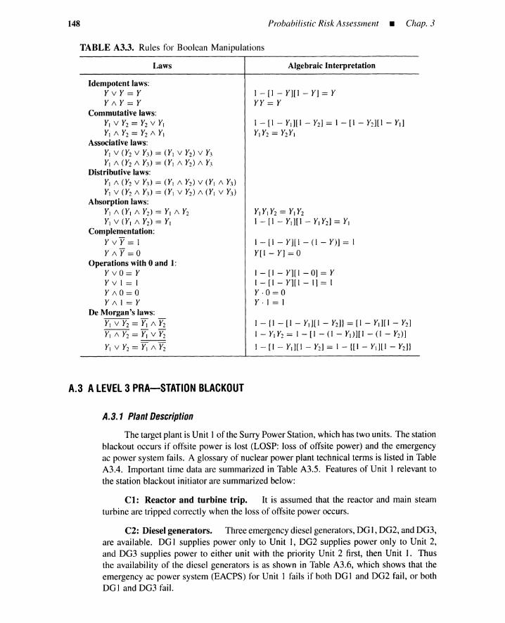
148 Probabilistic Risk Assessment _ Chap. 3
TABLE A3.3. Rules for Boolean Manipulations
Laws Algebraic Interpretation
Idempotent laws:YvY=YYI\Y=Y
Commutative laws:YI v Y2 = Y2 V YI
YI 1\ Y2 = Y2 1\ YI
Associative laws:YI v (Y2 V Y.~) = (Y I v Y2) v Y:~
YI 1\ (Y2 1\ Y3) = (Y I 1\ Y2) 1\ Y3
Distributive laws:YI 1\ (Y2 v Y3) = (Y I 1\ Y2) V (Y I 1\ Y3)
YI v (Y2 1\ Y3) = (Y I v Y2) 1\ (Y I v Y3)
Absorption laws:YI 1\ (Y I 1\ Y2) = YI 1\ Y2
YI V (YI 1\ Y2) = YI
Complementation:YvY = 1YI\Y=O
Operations with 0 and 1:YvO = YYvl=lYI\O=OYI\I=Y
De Morgan's laws:YI v Y2 = ~ 1\ Y2
YI 1\ Y2 = ~ V Y2
YI V Y2 = ~ 1\ Y2
1 - [I - Y][I - Y] = YYY = Y
1 - [I - Ytl[ 1 - Y2] = 1 - [I - Y2U1 - YtlYI Y2 = Y2YI
YI YI Y2 = YI Y2
1 - [I - Ytl[ 1 - YI Y2] = YI
1- [I - Y][I- (I - V)] = 1Y[I - Y] = 0
1 - [I - Y][I - 0] = Y1 - [I - YHI - 1] = IY -0=0Y-I = I
1- {I- [1- Ytl[l- Y2]} = [1- Ytl[l- Y2]
1- Y1Y2 = 1- [I - (1- YdHI - (1- Y2) ]
1 - [I - Yd[1 - Y2] = I - HI - Yd[l - Y2]}
A.3 ALEVEL 3 PRA-STATION BLACKOUT
A.3.1 Plant Description
The target plant is Unit 1of the Surry Power Station, which has two units. The stationblackout occurs if offsite power is lost (LOSP: loss of offsite power) and the emergencyac power system fails. A glossary of nuclear power plant technical terms is listed in TableA3.4. Important time data are summarized in Table A3.5. Features of Unit 1 relevant tothe station blackout initiator are summarized below:
Cl: Reactor and turbine trip. It is assumed that the reactor and main steamturbine are tripped correctly when the loss of offsite power occurs.
C2: Dieselgenerators. Three emergency diesel generators, DG 1, DG2, and DG3,are available. DG I supplies power only to Unit I, DG2 supplies power only to Unit 2,and DG3 supplies power to either unit with the priority Unit 2 first, then Unit 1. Thusthe availability of the diesel generators is as shown in Table A3.6, which shows that theemergency ac power system (EACPS) for Unit 1 fails if both DG 1 and DG2 fail, or bothDG] and DG3 fail.

Appendix A.3 • A Level 3 PRA-Station Blackout
TABLE A3.4. Glossary for Nuclear Power Plant PRA
149
Abbreviation
acAFWSAPETBWSCCICMCSTDOEACPSECCSFOFSFTOHPISHPMELOCALOSPNREC-AC-30OPPORVPWRRCIRCPRCSSBOSOSOlSRVTAFUTAFVB
Description
Alternating currentAuxiliaryfeedwatersystemAccidentprogression event treeBackupwater supplyCore-concrete interactionCore meltCondensatestorage tankDiesel generatorEmergency ac powersystemEmergency core-cooling systemFailureof operatorFailure to startFailure to operateHigh-pressure injectionsystemHigh-pressure melt ejectionLoss of coolant accidentLoss of offsitepowerFailure to restoreac power in 30 minOffsite powerPressure-operated relief valvePressurized water reactorReactorcoolant integrityReactorcoolant pumpReactorcoolant systemStation blackoutSteam generatorSteam generatorintegritySafety-reliefvalve(secondaryloop)Top of activefuelUncovering of top of active fuelVessel breach
TABLE A3.5. Time Data for Station Blackout PRA
Event
Condensatestorage tank (CST)depletionUncovering of top of activefuel
Start of core-coolantinjection
Time Span
1 hr1 hr
30 min
Condition
SRV sticks open1. Steam-driven AFWS failure2. Motor-driven AFWSfailureAfter ac power recovery
C3: Secondary loop pressure relief. In a station blackout (SBO), a certain amountof the steam generated in the steam generators (SGs) is used to drive a steam-driven AFWSpump (see description ofC5). The initiating LOSP causes isolation valves to close to preventthe excess steam from flowing to the main condenser. Pressure relief from the secondarysystem takes place through one or more of the secondary loop safety-relief valves (SRVs).
C4: AFWS heat removal. All systems capable of injecting water into the reactorcoolant system (RCS) depend on pumps driven by ac motors. Thus if decay heat cannot be

150 Probabilistic Risk Assessment • Chap. 3
TABLE A3.6. Emergency Power Availability for Units 1 and 2
DGI DG2 DG3 Unit 1 Power Unit 2 Power
UP UP UP OK OKUP UP DOWN OK OKUP DOWN UP OK OKUP DOWN DOWN OK NOT OKDOWN UP UP OK OKDOWN UP DOWN NOT OK OKDOWN DOWN UP NOT OK OKDOWN DOWN DOWN NOT OK NOT OK
removed from the RCS, the pressure and temperature of the water in the RCS will increaseto the point where it flows out through the pressure-operated relief valves (PORVs), andthere will be no way to replace this lost water. The decay heat removal after shutdown isaccomplished in the secondary loop via steamgenerators, that is, heatexchangers. However,if the secondary loop safety-relief valves repeatedly open and close, and the water is lostfrom the loop, then the decay heat is removed by the AFWS, which injects water into thesecondary loop to remove heat from the steam generators.
C5: AFWS trains. The AFWS consists of three trains, two of which have ac-motor-driven pumps, and one train that has a steam-turbine-driven pump. With the loss ofac power (SBO), the motor-driven trains will not work. The steam-driven train is availableas long as steam isgenerated in the steam generators (SGs), and de battery power is availablefor control purposes.
C6: Manual valve operation. If one or more of the secondary loop SRVs fails,water is lost from the secondary loop at a significant rate. The AFWS draws water fromthe 90,OOO-gallon condensate storage tank (CST). If the SRVsticks open, the AFWS drawsfrom the CST at 1500 gpm to replace the water lost through the SRV, thus depleting theCST in one hour. A 3oo,OOO-gallon backup water supply (BWS) is available, but the AFWScannot draw from this tank unless a valve is opened manually. If the secondary loop SRVcorrectly operates, then the water loss is not significant.
C7: Core uncovering. With the failure of the steam-driven AFWS, and no acpower to run the motor-driven trains, the ReS heats up until the pressure forces steamthrough the PORVs. Water loss through the PORVs continues, with the PORVs openingand closing, until enough water has been lost to reduce the liquid water level below the topof active fuel (TAF). The uncoveringof the top of active fuel (UTAF)occurs approximately60 min after the three AFWS train failures. The onset of core degradation follows shortlyafter the UTAF.
C8: AC power recovery. A 30-min time delay is assumed from the time that acpower is restored to the time that core-coolant injection can start. Thus, ac power mustbe recovered within 30 min after the start of an AFWS failure to prevent core uncovering.There are two recovery options from the loss of ac power. One is the restoration of offsitepower, and the other is recovery of a failed diesel generator (DG).
A.3.2 Event Tree forStation Blackout
Figure A3.8 shows a portion of an event tree for initiating event SBO at Unit 1.

Appendix A.3 • A Level 3 PRA-Station Blackout 151
I --~I
sao at NREC- RCI SGI AFWSUnit 1 AC-30
I - II I
T U a as L NO CoreI -- II I
1 OK
2 OK
I II II I
12 CM
13 OK
I II II I
19 CM
20 OK
I II II I
22 CM
I I---- I I
I I
25 CM
Figure A3.8. Station blackout event tree.
Event-tree headings. The event tree has the following headings and labels.
1. SBO at Unit 1 (T): This initiating event is defined by failure of offsite power, andfailure of emergency diesel power supply to Unit 1.
2. NREC-AC-30 (U): This is a failure to recover ac power within 30 min, wheresymbols N, REC, and AC denote No, Recovery, and ac power, respectively.
3. RCI (Q): This is a failure of reactor-coolant integrity. The success of RCI meansthat the PORVs operate correctly and do not stick open.
4. SGI (QS): This denotes steam-generator integrity at the secondary loop side. Ifthe secondary loop SRVs stick open, this failure occurs.
5. AFWS (L): This is an AFWS failure. Note that this failure can occur at differentpoints in time. If the steam turbine pump fails to start, then the AFWS failureoccurs at 0 min, that is, at the start of the initiating event. The description of C7 inSection A.3.1 indicates that the fuel uncovering occurs in approximately 60 min;C8 shows there is a 30-min time delay for re-establishing support systems; thus acpower must be recovered within 30 min after the start of the initiating event, whichjustifies the second heading NREC-AC-30. On the other hand, if the steam turbinepump starts correctly, the steam-driven AFWS runs until the CST is depleted inabout 60 min under SRV failures. The AFWS fails at that time if the operators failto switch the pump suction to the BWS. In this case, ac power must be recovered

152 Probabilistic Risk Assessment _ Chap. 3
within 90 min because the core uncovering statts in 120 min and there is a 3D-mintime delay for coolant injection to prevent the core uncovering.
Note that the event tree in Figure A3.8 includes support-system failure, that is, stationblackout and recovery failure of ac power sources. The inclusion of support-system failurescan be made more systematically if a large ET/small Ff approach is used.
A.3.3 AccidenlSequences
An accident sequence is an initiating event followed by failure of the systems torespond to the initiator. Sequences are defined by specifying what systems fail to respondto the initiator. The event tree of Figure A3.8 contains the following sequences, some ofwhich lead to core damage.
Sequence 1. Station blackout occurs and there is a recovery within 30 min. ThePORVs and SRVs operate correctly, hence reactor coolant integrity and steam generatorintegrity are both maintained. AFWS continuously removes heat from the reactor, thuscore uncovering will not occur. One hour from the start of the accident, feed and bleedoperations are re-established because the ac power is recovered within 30 min, thus coredamage is avoided.
Sequence 2. Similar to sequence 1 except that ac power is recovered 1 hr fromthe start of accident. Core uncovering will not occur because heat removal by the AFWScontinues. Core damage does not occur because feed and bleed operations start within 1.5 hr.
Sequence 12. Ac power is not re-established within 30 min. The AFWS fails atthe very start of the accident because of a failure in the steam-turbine-driven AFWS train. Acore uncovering occurs after 1 hr because the feed and bleed operation by primary coolantinjection cannot be re-established within 1 hr.
Sequence 13. Ac power is not restored within 30 min. The reactor coolant integrityis maintained but steam generator integrity is not. However, AFWS continuously removesthe decay heat, providing enough time to recover ac power. Core damage is avoided.
Sequence 19. Similar to sequence 12 except that AFWS fails after 1 hr becausethe operators did not open the manual valve to switch the AFWS suction to a BWS. Thissequence contains an operator error. A core uncovering starts at 2 hr after the initiatingevent. Core damage occurs because feed and bleed operation cannot be re-establishedwithin 2 hr if the ac power "is not re-established within 1.5 hr.
Sequence 20. Similar to sequence 13 except that RCI, instead of the SGI, fails.Core damage is avoided because the AFWS continuously removes heat, thus preventing thereactor coolant from overheating.
Sequence 22. Similar to sequence 19 except that RCI, instead of the SGI, fails.Failure of AFWS results in core damage if ac power is not re-established in time.
Sequence 25. This is a more severe accident sequence than 19 or 22 because theRCI and SGI both fail, in addition to the AFWS failure. Core damage occurs.
A.3.4 Faull Trees
In an accident-frequency analysis, fault trees, down to the hardware level of detail,are constructed for each event-tree heading. Failure rates for equipment such as pumps andvalves are developed ideally from failure data specific to the plant being analyzed.
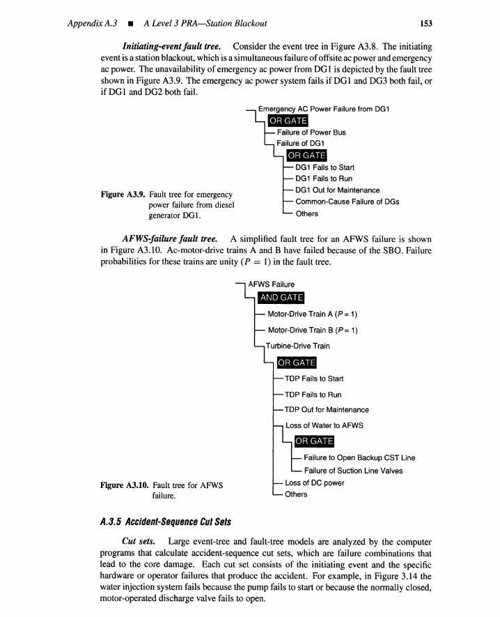
Appendix A.3 • A Level 3 PRA-Station Blackout 153
Initiating-event fault tree. Consider the event tree in Figure A3.8. The initiatingevent is a station blackout, which is a simultaneous failure of offsite ac power and emergencyac power. The unavailability of emergency ac power from DG 1 is depicted by the fault treeshown in Figure A3.9. The emergency ac power system fails if DG 1 and DG3 both fail, orif DG 1 and DG2 both fail.
Figure A3.9. Fault tree for emergencypower failure from dieselgenerator DG 1.
Emergency AC Power Failure from OG1...Failure of Power Bus
Failure of DG1-DG1 Fails to Start
DG1 Fails to Run
DG1 Out for Maintenance
Common-Cause Failure of DGs
Others
AFWS-failure fault tree. A simplified fault tree for an AFWS failure is shownin Figure A3.10. Ac-motor-drive trains A and B have failed because of the SBO. Failureprobabilities for these trains are unity (P = 1) in the fault tree.
AFWS Failure...Motor-Drive Train A (P = 1)
Motor-Drive Train B (P =1)
Turbine-Drive Train
TOP Fails to Start
TOP Fails to Run
TOP Out for Maintenance
Loss of Water to AFWS
Figure A3.10. Fault tree for AFWSfailure.
A.3.5 Accident-Sequence Cut Sets
Failure to Open Backup CST Line
Failure of Suction Line Valves
Loss of DC power
Others
Cut sets. Large event-tree and fault-tree models are analyzed by the computerprograms that calculate accident-sequence cut sets, which are failure combinations thatlead to the core damage. Each cut set consists of the initiating event and the specifichardware or operator failures that produce the accident. For example, in Figure 3.14 thewater injection system fails because the pump fails to start or because the normally closed,motor-operated discharge valve fails to open.

154 Probabilistic Risk Assessment _ Chap. 3
Sequence expression. Consider accident sequence 19 in Figure A3.8. The logicexpression for this sequence, according to the column headings, is
Sequence] 9 == T /\ V /\ Q /\ QS /\ L, (A.53)
where Qindicates not-Q, or success and symbol ,« is a logic conjunction (a Boolean AND).System-success states like Q are usually omitted during quantification if the state resultsfrom a single event, because the success values are close to 1.0 in a well-designed system.Success state Qmeans that all RCS PORVs successfully operate during the SBO, thusensuring reactor coolant integrity.
Heading analysis. Headings T, V, Q, QS, and L are now considered in more detail.
1. Heading T denotes a station blackout, which consists of offsite power failure andloss of emergency power. The emergency power fails if DG 1 and DG3 both failor if DG 1 and DG2 both fail. The fault tree in Figure A3.9 indicates that DG 1fails because of failure to start, failure to run, out of service for maintenance,common-cause failure, or others. DG3 fails similarly.
2. Heading V is a failure to restore ac power within 30 min. This occurs when neitheroffsite nor emergency ac power is restored. Emergency ac power is restored whenDG 1 OR (DG2 AND DG3) are functional.
3. Heading Q is a reactor coolant integrity failure.
4. Heading QS is a steam generator integrity failure at the secondary side. Thisoccurs if an SRV in the secondary system is stuck open.
5. Heading L is an AFWS failure. For accident sequence 19, this failure occurs 1hr after the start of the accident when the operators fail to open a manual valve toswitch the AFWS pump suction to backup condensate water storage tank, BWS.
Timing consideration. Note here that the AFWS time to failure is I hr for sequence19. A core uncovering starts after 2 hr. Thirty minutes are required for re-establishing thesupport systems after an ac power recovery. Thus accident sequence 19 holds only if acpower is not recovered within 1.5 hr. This means that NREC-AC-30 should be rewritten asNREC-AC-90. It is difficult to do a PRA without making mistakes.
Sequence cut sets. A cut set for accident sequence 19 defines a combination offailures that leads to the accident. There are 216 of these cut sets. From the above section,"Heading Analysis," starting with T, a cut set C I consisting of nine events is defined. Theevents-and their probabilities-are
1. LOSP (0.0994): An initiating-event element, that is, loss of offsite power, with anannual failure frequency of 0.0994.
2. FS-DG I (0.0133): DG 1 fails to start.
3. FTO-DG2 (0.966): Success of DG2. Symbol FTO (fails to operate) includes afailure to start. The DG2 failure implies additional SBO for Unit 2, yielding amore serious situation.
4. FS-DG3 (0.0133): DG3 fails to start.
5. NREC-OP-90 (0.44): Failure to restore offsite electric power within 1.5 hr.
6. NREC-DG-90 (0.90): Failure to restore DG within 1.5 hr.
7. R-PORV (0.973): RCS PORVs successfully close during SBO.
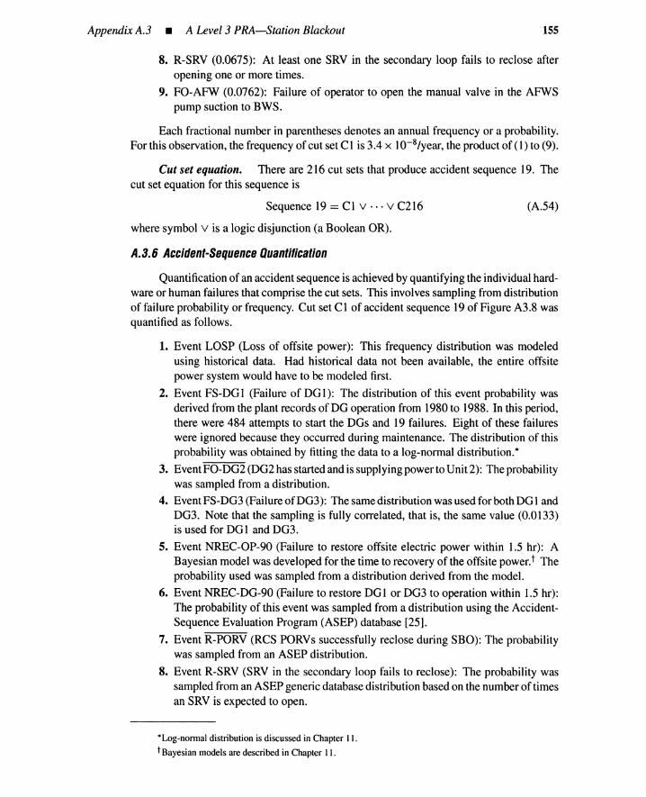
Appendix A.3 • A Level 3 PRA-Station Blackout 155
8. R-SRV (0.0675): At least one SRV in the secondary loop fails to reclose afteropening one or more times.
9. FO-AFW (0.0762): Failure of operator to open the manual valve in the AFWSpump suction to BWS.
Each fractional number in parentheses denotes an annual frequency or a probability.For this observation, the frequency of cut set C1 is 3.4 x 10⁻⁸/year, the product of (1) to (9).
Cut set equation. There are 216 cut sets that produce accident sequence 19. Thecut set equation for this sequence is
Sequence 19 = Cl v ... v C216
where symbol v is a logic disjunction (a Boolean OR).
A.3.6 Accident-Sequence Quantification
(A.54)
Quantification of an accident sequence is achieved by quantifying the individual hard-ware or human failures that comprise the cut sets. This involves sampling from distributionof failure probability or frequency. Cut set Cl of accident sequence 19 of Figure A3.8 wasquantified as follows.
1. Event LOSP (Loss of offsite power): This frequency distribution was modeledusing historical data. Had historical data not been available, the entire offsitepower system would have to be modeled first.
2. Event FS-DG 1 (Failure of DG 1): The distribution of this event probability wasderived from the plant records of DG operation from 1980 to 1988. In this period,there were 484 attempts to start the DGs and 19 failures. Eight of these failureswere ignored because they occurred during maintenance. The distribution of thisprobability was obtained by fitting the data to a log-normal distribution.*
3. Event FO-DG2 (DG2 has started and is supplying power to Unit 2): The probabilitywas sampled from a distribution.
4. Event FS-DG3 (Failure ofDG3): The same distribution was used for both DG 1andDG3. Note that the sampling is fully correlated, that is, the same value (0.0133)is used for DO 1 and D03.
5. Event NREC-OP-90 (Failure to restore offsite electric power within 1.5 hr): ABayesian model was developed for the time to recovery of the offsite power.t Theprobability used was sampled from a distribution derived from the model.
6. Event NREC-DG-90 (Failure to restore DG 1 or DG3 to operation within 1.5 hr):The probability of this event was sampled from a distribution using the Accident-Sequence Evaluation Program (ASEP) database [25].
7. Event R-PORV (RCS PORVs successfully reclose during SBO): The probabilitywas sampled from an ASEP distribution.
8. Event R-SRV (SRV in the secondary loop fails to reclose): The probability wassampled from an ASEP generic database distribution based on the number of timesan SRV is expected to open.
*Log-normal distribution is discussed in Chapter 11.
t Bayesian models are described in Chapter 11.

156 Probabilistic Risk Assessment _ Chap. 3
9. FO-AFW (Failure of operator to open the manual valve from the AFWS pumpsuction to BWS): The probability was sampled from a distribution derived usinga standard method for estimating human reliability. This event is a failure to suc-cessfully complete a step-by-step operation following well-designed emergencyoperating procedures under a moderate level of stress.*
A.3.7 Accident-Sequence Group
ASG. An accident-frequency analysis identifies significant accident sequences,whichcan be numerous. The accident-progressionanalysis, whichis a complexand lengthyprocess,can besimplifiedifaccidentsequencesthatprogressina similarfashionaregroupedtogether as ASGs. For example, sequences 12, 19, and 22 in Figure A3.8 can be groupedin the same ASG.
Cut sets and effects. A cut set consists of specific hardware faults and operatorfailures. Many cut sets on an accident sequence are essentially equivalent because thefailure mode is irrelevant. Thus equivalent cut sets can be grouped together in an ASG. Intheory, it is possible that the cut sets from a single accident sequence are separable into two(or more) different groups. However, this happens only rarely. Grouping into ASGs canusually be performed on an accident-sequence level.
For example, referring to Figure A3.9, it would make little difference whether thereis no ac power because DG1 is out of service for maintenance or whether DG1 failed tostart. The fault is different, and the possibilities for recoverymay be different, but the resulton a system level is the same. Exactly how DG1 failed must be known to determine theprobability of failure and recovery, but it is less important in determining how the accidentprogresses after UTAF. Most hardware failures underan OR gate are equivalent in that theylead to the same top event.
A.3.8 Uncertainty Analysis
Because component-failureand human-errorprobabilitiesare sampled from distribu-tions, the quantification process yields a distributionof occurrenceprobabilitiesfor each ac-cident sequence. Four measures are commonly used for the accident-sequence-probabilitydistribution: mean, median, 5th percentile value, and 95th percentile value.
A.3.9 Accident-Progression Analysis
A.3.9.1 Accident-progression event tree. This analysis is basedon an APET.Eachevent-tree heading on an APET corresponds to a question relating to an ASG. Branchingoperationsare performedafter each question. Branchingratiosand parameter valuesare de-termined by expert panels or computercodes. Examplesof parameters includecontainmentpressure before vessel breach, containment pressure rise at vessel breach, and containmentfailurepressure. The followingquestionsforsequence 19or accident-sequencegroupASG1illustrate accident-progression analysis based on APET. Some questions are not listed forbrevity. Each question is concerned with core recovery prior to vessel breach, in-vesselaccident progression, ex-vessel accident progression, or containment building integrity.
1. ReS integrity at UTAF? Accident-sequence group ASG1 involves no ReSpressure boundary failure. A relevant branch, "PORVs do not stick open," ischosen.
*Human reliability analysis is described in Chapter 10.

Appendix A.3 • A Level 3 PRA-Station Blackout 157
2. AC power status? ASG 1indicates that ac power is available throughout the plantif offsite power is recovered after UTAF. Recovery of offsite power after the onsetof core damage but before vessel failure is more likely than recovery of powerfrom the diesel generators. Recovery of power would allow the high-pressureinjection system (HPIS) and the containment sprays to operate and prevent vesselfailure. One progression path thus assumes offsite ac power recovery beforevessel failure; the other path does not.
3. Heat removal from SGs? The steam-turbine-driven AFWS must fail for acci-dent-sequence group ASG 1 to occur, but the electric-motor-driven AFWS isavailable when power is restored. A relevant branch is taken to reflect thisavailability.
4. Cooling for RCP seals? Accident-sequence group ASG 1 implies no coolingwater to the RCP seals, so there is a LOCA risk by seal failure unless ac poweris available.
5. Initial containment failure? The containment is maintained below atmosphericpressure. Pre-existing leaks are negligible and the probability of a containmentfailure at the start of the accident is 0.0002. There are two possible branches.The more likely branch, no containment failure, is followed in this example.
6. RCS pressure at UTAF? The RCS must be at the setpoint pressure of the PORVs,about 2500 psi. The branch indicating a pressure of 2500 psi is followed.
7. PORVs stick open? These valves will need to operate at temperatures well inexcess of design specifications in the event of an AFWS failure. They may fail.The PORVs reclose branch is taken.
8. Temperature-induced RCP seal failure? If a flow of relatively cool waterthrough the seal is not available, the seal material eventually fails. In accidentsequence 19, seal failure can only occur after UTAF, which starts at 2 hr. Whetherthe seals fail or not determines the RCS pressure when the vessel fails. Thecontainment loads at VB (vessel breach) depend strongly on the RCS pressure atthat time. There are two possibilities, and seal failure is chosen.
9. Temperature-induced steam generator tube rupture? If hot gases leaving thecore region heat the steam generator tubes sufficiently, failure of the tubes occurs.The expert panel concluded that tube rupture is not possible because the failureof the RCP seals has reduced the RCS pressure below the setpoint of the PORVs.
10. Temperature-induced hot leg failure? There is no possibility of this failurebecause the RCS pressure is below the setpoint of the PORVs.
11. AC power early? The answer to this question determines whether offsite poweris recovered in time to restore coolant injection to the core before vessel failure.A branch that proceeds to vessel breach is followed in this example.
12. RCS pressure at VB? It is equally likely that the RCS pressure at VB is in a highrange, an intermediate range, or a low range. In this example, the intermediaterange was selected.
13. Containment pressure before VB? The results of a detailed simulation indicatedthat the containment atmospheric pressure will be around 26 psi. Parameter PIis set at 26 psi.
14. Water in reactor cavity at VB? There is no electric power to operate the spraypumps in this blackout accident; the cavity is dry at VB in the path followed inthis example.

158 Probabilistic Risk Assessment _ Chap. 3
15. Alpha-mode failure? This is a steam explosion (fuel-coolant interaction) in thevessel. The path selected for this example is "no alpha-mode failure."
16. Type of vessel breach? The possible failure modes are pressurized ejection,gravity pour, or gross bottom head failure. Pressurized ejection after vesselbreach is selected.
17. Size of hole in vessel? The containment pressure rise depends on hole size.There are two possibilities: small hole and large hole. This example selects thelarge hole.
18. Pressure rise at VB? Pressure, P2 == 56.8 psi, is selected.
19. Ex-vessel steam explosion? A significant steam explosion occurs when thehot core debris falls into water in the reactor cavity after vessel breach. In thisexample, the cavity is dry, so there is no steam explosion.
20. Containment failure pressure? This example selects a failure pressure of P3 ==163.1 psi.
21. Containment failure? From question 13, containment pressure before VB isPI == 26 psi. From question 18, pressure rise at VB is P2 == 56.8 psi. Thus theload pressure, PI + P2 == 82.8 psi, is less than the failure pressure P3 == 163.1,so there is no containment failure at vessel breach.
22. AC power late? This question determines whether offsite power is recoveredafter vessel breach, and during the initial CCI (core-concrete interaction) period.The initial CCI period means that no appreciable amount of hydrogen has beengenerated by the CCI. This period is designated the "Late" period. Power recoveryis selected.
23. Late sprays? Containment sprays now operate because the power has beenrestored.
24. Late burn? Pressure rise? The restoration ofpower means that ignition sourcesmay be present. The sprays condense most of the steam in the containment andmay convert the atmosphere from one that was inert because of the high steamconcentration to one that is flammable. The pressure rise question asks "whatis the total pressure that results from the ensuing deflagration?" For the currentexample, the total load pressure is P4 == 100.2 psi.
25. Containment failure and type of failure? The failure pressure is P3 == 163.1psi. The load pressure is P4 == 100.2 psi, so there is no late containment failure.
26. Amount of core in CCI? The path being followed has pressurized ejection at VBand a large fraction of the core ejected from the vessel. Pressurized ejection meansthat a substantial portion of the core material is widely distributed throughout thecontainment. For this case, it is estimated that between 30% and 70% of the corewould participate in CCI.
27. Does prompt CCI occur? The reactor cavity is dry at VB because the spraysdid not operate before VB, so CCI begins promptly. If the cavity is dry atVB, the debris will heat up and form a noncoolable configuration; even if wateris provided at some later time, the debris will remain hot. Thus prompt CCIoccurs.
28. Very large ignition? Because an ignition source has been present since thelate bum, any hydrogen that accumulates after the bum will ignite whenever aflammable concentration is reached. Therefore, the ignition branch is not taken.

Appendix A.3 • A Level 3 PRA-Station Blackout 159
29. Basemat melt-through? It is judged that eventual penetration of the basemat bythe CCI has only a 5% probability. However, the basemat melt-through branchis selected because the source-term analysis in Section A.3.9.3 and consequenceanalyses in Section A.3.9.4 are not of much interest if there is no failure of thecontainment.
30. Final containment condition? This summarizes the condition of the contain-ment a day or more after the start of the accident. In the path followed through theAPET, there were no aboveground failures, so basemat melt-through is selected.
A.3.9.2 Accident-progression groups. There are so many paths through the APETthat they cannot all be considered individually in a source-term analysis. Therefore, thesepaths are condensed into APGs.
For accident sequence 19,22 APGs having probabilities above 10-7 exist. For ex-ample, the alpha-mode steam explosion probability is so low that all the alpha-mode pathsare truncated and there are no accident-progression groups with containment alpha-modefailures. The most probable group, with probability 0.55, has no VB and no containmentfailure. It results from offsite ac power recovery before the core degradation process hadgone too far (see the second question in Section A.3.9.1).
An accident-progression group results from the path followed in the example in Sec-tion A.3.9.1. It is the most likely (0.017) group that has both VB and containment failures.Basemat melt-through occurs a day or more after the start of the accident. The group ischaracterized by:
1. containment failure in the final period
2. sprays only in the late and very late periods
3. prompt CCI, dry cavity
4. intermediate pressure in the RCS at VB
5. high-pressure melt ejection (HPME) occurred at VB
6. no steam-generator tube rupture
7. a large fraction of the core is available for CCI
8. a high fraction of the Zr is oxidized
9. high amount of core in HPME
10. basemat melt-through
11. one effective hole in the RCS after VB
A.3.9.3 Source-term analysis
Radionuclide classes. A nuclear power plant fuel meltdown can release 60 ra-dionuclides. Some radionuclides behave similarly both chemically and physically, so theycan be considered together in the consequence analysis. The 60 isotopes comprise nine ra-dionuclide classes: inert gases, iodine, cesium, tellurium, strontium, ruthenium, lanthanum,cerium, and barium. There are two types of releases: an early release due to fission productsthat escape from the fuel while the core is still in the RCS, that is, before vessel breach; anda late release largely due to fission products that escape from the fuel after VB.
Early- and late-release fractions. The radionuclides in the reactor and their decayconstant are known for each class at the start of the source-term analysis. For an accident-progression group, the source-term analysis yields the release fractions for each radionuclide

160 Probabilistic Risk Assessment _ Chap. 3
class. These fractions are estimated for the early and late releases. Radionuclide inventorymultiplied by an early-release fraction gives the amount released from the containment inthe early period. A late release is calculated similarly.
Consider as an example the release fraction ST for an early release of iodine. Thisfraction consists of three subfractions and one factor that describes core, vessel, containment,and environment:
ST == [FCOR x FVES x FCONV/DFE] +OTHERS
where
1. FCOR: fraction of the core iodine released in the vessel before VB
2. FVES: fraction of the iodine released from the vessel
3. FCONV: fraction of the iodine released from the containment
4. DFE: decontamination factor (sprays, etc.)
(A.55)
These subfractions and the decontamination factor are established by an expert paneland reflect the results of computer codes that consider chemical and physical properties offission products, and flow and temperature conditions in the reactor and the containment.For instance, sample data such as FeOR =0.98, FVES = 0.86, FCONV = 10-6, OTHERS= 0.0, and DFE =34.0 result in ST =2.5 x ]0-8 . The release fraction ST is a very smallfraction of the original iodine core inventory because, for this accident-progression group,the containment failure takes place many hours after VB and there is time for natural andengineered removal processes to operate.
Early- and late-release fractions are shown in Table A3.7 for a source-term groupcaused by an accident-progression group dominated by a late release.
TABLE A3.7. Early and Late Release Fractionsfor a Source Term
Fission Early Late TotalProducts Release Release Release
Xe, Kr 0.0 1.0 1.0I 0.0 4.4£-3 4.4£-3CS,Rb 0.0 8.6£-8 8.6£-8Te,Sc,Sb 0.0 2.3£-7 2.3£-7Ba 0.0 2.8£-7 2.8£-7Sr 0.0 1.2£-9 1.2£-9Ru, etc. 0.0 3.0£-8 3.0£-8La, etc. 0.0 3.1£-8 3.1£-8Ce, Np, Pu 0.0 2.0£-7 2.0£-7
Other characteristics of source terms. The source-term analysis calculates forearly and late releases: start times, durations, height of release source, total energy. Eachrelease involves nine isotope groups.
Partitioning into source-term groups. The accident-frequency analysis yields acci-dent-sequence groups. Each accident-sequence group is associated with many accident-progression groups developed through APET. Each accident-progression group yields sourceterms. For instance, a NUREG-1150 study produced a total of 18,591 source terms from
Appendix A.3 • A Level 3 PRA-Station Blackout 161
all progression groups. This is far too many, so a reduction step must be performed beforea consequence analysis is feasible. This step is called a partitioning.
Source terms having similar adverse effects are grouped together. Two types ofadverse effects are considered here: early fatality and chronic fatality. These adverseeffects are caused by early and late fission product releases.
Early fatality weight. Each isotope class in a source term is converted into anequivalent amount of 131 I by considering the following factors for the early release and laterelease.
1. Isotope conversion factor
2. Inventory of the isotope class at the start of the accident
3. Release fraction
4. Decay constant for the isotope class
5. Start of release
6. Release duration
The early-fatality weight factor is proportional to the inventory and release fraction.Because a source term contains nine isotope classes, a total early fatality weight for thesource term is determined as a sum of 9 x 2 = 18 weights for early and late releases.
Chronic fatality weight. This is calculated for each isotope class in a source termby considering the following.
1. Inventory of the isotope class at the start of the accident
2. Release fractions for early and late releases
3. Number of latent cancer fatalities due to early exposure from an isotope class,early exposure being defined as happening in the first seven days after the accident
4. Number of latent cancer fatalities due to late exposure from an isotope class, lateexposure being defined as happening after the first seven days
Note that the early release, in theory, also contributes to the late exposure to a certainextent because of residual contamination.
The chronic-fatality weight factor is proportional to inventory, release fractions, andnumber of cancer fatalities. Each source term contains nine isotope classes, and thus hasnine chronic fatality weights. A chronic fatality weight for the source terms is a sum ofthese nine weights.
Evacuation timing. Recall that each source term is associated with early releasestart time and late release start time. The early and late releases in a source term are classifiedinto categories according to evacuation timings that depend on the start time of the release.(In reality everybody would run as fast and as soon as they could.)
1. Early evacuation: Evacuation can start at least 30 min before the release begins.
2. Synchronous evacuation: Evacuation starts between 30 min before and 1 hr afterthe release begins.
3. Late evacuation: Evacuation starts one or more hours after the release begins.
Stratified grouping. Each source term now has three attributes: early fatalityweight, chronic fatality weight, and evacuation timing. The three-dimensional space isnow divided into several regions. Source terms are grouped together if they are in the same
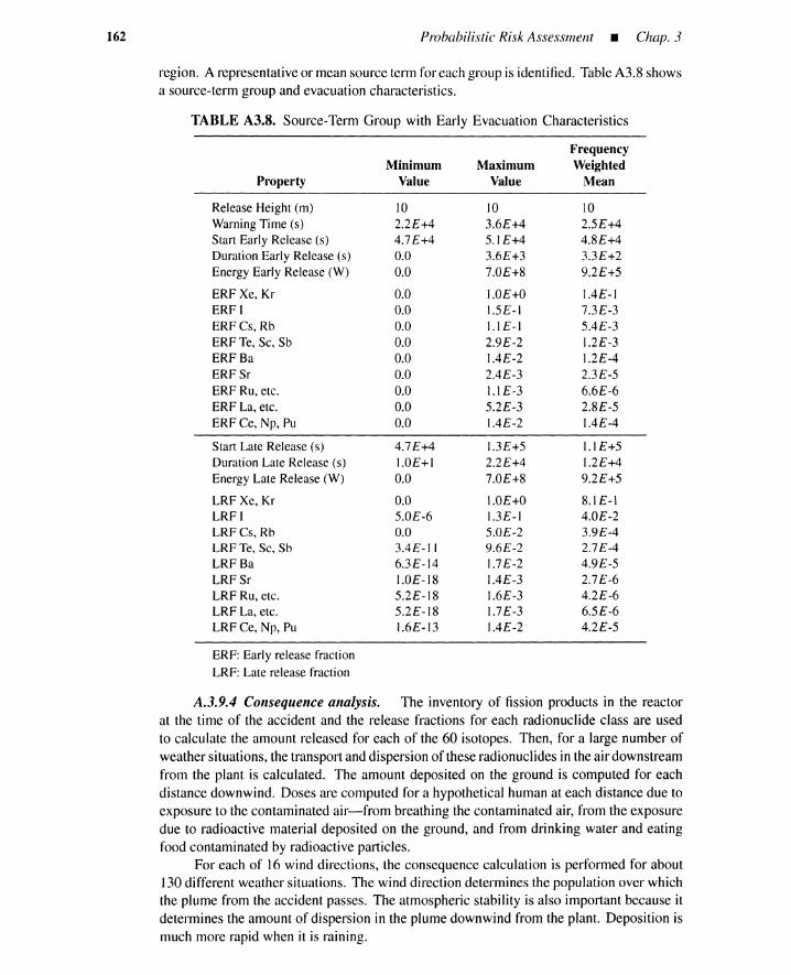
162 Probabilistic Risk Assessment • Chap. 3
region. A representativeor mean source term for each group is identified. TableA3.8 showsa source-term group and evacuation characteristics.
TABLE A3.8. Source-Term Group with Early Evacuation Characteristics
FrequencyMinimum Maximum Weighted
Property Value Value Mean
Release Height (m) 10 10 10Warning Time (s) 2.2£+4 3.6£+4 2.5£+4Start Early Release (s) 4.7£+4 5.1£+4 4.8£+4Duration Early Release (s) 0.0 3.6£+3 3.3£+2Energy Early Release (W) 0.0 7.0£+8 9.2£+5
ERF Xe, Kr 0.0 1.0£+0 1.4£-1ERFI 0.0 1.5£-1 7.3£-3ERFCs, Rb 0.0 1.1 £-1 5.4£-3ERF Te, Sc, Sb 0.0 2.9£-2 1.2£-3ERFBa 0.0 1.4£-2 1.2£-4ERF Sr 0.0 2.4£-3 2.3£-5ERF Ru, etc. 0.0 1.1 £-3 6.6£-6ERF La, etc. 0.0 5.2£-3 2.8£-5ERF Ce, Np, Pu 0.0 1.4£-2 1.4£-4
Start Late Release (s) 4.7£+4 1.3£+5 1.1 £+5Duration Late Release (s) 1.0£+1 2.2£+4 1.2£+4Energy Late Release (W) 0.0 7.0£+8 9.2£+5
LRF Xe, Kr 0.0 1.0£+0 8.1£-1LRFI 5.0£-6 1.3£-1 4.0£-2LRFCs, Rb 0.0 5.0£-2 3.9£-4LRF Te, Sc, Sb 3.4£-11 9.6£-2 2.7£-4LRFBa 6.3£-14 1.7£-2 4.9£-5LRFSr 1.0£-18 1.4£-3 2.7£-6LRF Ru, etc. 5.2£-18 1.6£-3 4.2£-6LRF La, etc. 5.2£-18 1.7£-3 6.5£-6LRF Ce, Np, Pu 1.6£-13 1.4£-2 4.2£-5
ERF: Early release fractionLRF: Late release fraction
A.3.9.4 Consequence analysis. The inventory of fission products in the reactorat the time of the accident and the release fractions for each radionuclide class are usedto calculate the amount released for each of the 60 isotopes. Then, for a large number ofweather situations, the transport and dispersion of these radionuclides in the air downstreamfrom the plant is calculated. The amount deposited on the ground is computed for eachdistance downwind. Doses are computed for a hypothetical human at each distance due toexposure to the contaminated air-from breathing the contaminated air, from the exposuredue to radioactive material deposited on the ground, and from drinking water and eatingfood contaminated by radioactive particles,
For each of 16 wind directions, the consequence calculation is performed for about130different weather situations. The wind direction determines the population over whichthe plume from the accident passes. The atmospheric stability is also important because itdetermines the amount of dispersion in the plume downwind from the plant. Deposition ismuch more rapid when it is raining.

Chap. 3 • Problems 163
Table A3.9 shows a result of consequence analysis for a source-term group. Theseconsequences assume that the source term has occurred. Different results are obtained fordifferent weather assumptions. Figure 3.19 shows latent cancer fatality risk profiles. Eachprofile reflects uncertainty caused by weather conditions, given a source-term group; the95%, 5%, mean, and median profiles represent uncertainty caused by variations of basiclikelihoods.
TABLE A3.9. Result of Consequence Analysis for a Source-Term Group
Early FatalitiesEarly InjuriesLatent Cancer FatalitiesPopulation Dose-SO miPopulation Dose-regionEconomic Cost (dollars)Individual Early Fatality Risk-l miIndividual Latent Cancer Fatality Risk-IO mi
A.3.10 Summary
0.04.2£-61.1£+22.7£+S person-rem6.9£+S person-rem1.8£+80.07.6£-S
A level 3 PRA for a station-blackout initiating event was developed. First, an event treeis constructed to enumerate potential accident sequences. Next, fault trees are constructedfor the initiating event and mitigation system failures. Each sequence is characterizedand quantified by accident sequence cut sets that include timing considerations. Accident-sequence groups are determined and an uncertainty analysis is performed for a level 1PRA.
An accident-progression analysis is performed using an accident-progression eventtree (APET), which is a question-answering technique to determine the accident-progressionpaths. The APET output is grouped in accident-progression groups and used as the inputto a source-term analysis. This analysis considers early and late releases. The relativelysmall number of source-term groups relate to early fatality weight, chronic fatality weight,and evacuation timing. A consequence analysis is performed for each source-term groupusing different weather conditions. Risk profiles and their uncertainty are determined.
PROBLEMS
3.1. Give seven basic tasks for a reactor safety study (WASH-1400).
3.2. Give five tasks for WASH-1400 update, NUREG-llS0. Identify three PRA levels.
3.3. Compare PRA applications to nuclear reactor, railway, oil tanker, and disease problems.
3.4. Enumerate seven major and three supporting activities for a level 1 PRA.
3.5. Briefly discuss benefits and detriments of PRA
3.6. Explain the following concepts: 1) hazardous energy sources, 2) hazardous process andevents, 3) generic failure modes.
3.7. Give examples of guide words for HAZOPS.
3.8. Figure P3.8 is a diagram of a domestic hot-water system (Lambert, UCID-16328, May1973). The gas valve is operated by the controller, which, in turn, is operated by thetemperature measuring and comparing device. The gas valve operates the main burnerin full-onlfull-off modes. The check valve in the water inlet prevents reverse flow due tooverpressure in the hot-water system, and the relief valve opens when the system pressureexceeds 100 psi.

164 Probabilisti c Risk Assessment _ Chap. 3
Hot Water Faucet(normally closed)
PressureRelief Valve
FlueGases
tCold
Water
CheckValve
TemperatureMeasuring
andCompa ring
Device
StopValve
Gas -:::::::====1t9<J================~
Figure P3.8. Schematicof domestic hot water system.
Control of the temperature is achieved by the controller opening and closing themaingas valvewhen the water temperature goes outside the preset limits (1400-1 80°F).The pilot light is alwayson.(a) Formulate a list of undesired safety and reliability events.(b) Do a preliminary hazardanalysis on the system.(c) Do a failure modesand effectsanalysis.(d) Do a qualitative criticality ranking.
3.9. (a) Suppose we are presented with two indistinguishable ums. Urn I contains 30 redballsand 70 green ones, and Urn2 contains50 red ballsand 50 green ones. One urnis selected at random and a ball withdrawn. What is the probability that the ball isred?
(b) Suppose the ball drawn was red. What is the probability of its being from Urn I?

ault-Tree Construction
4.1 INTRODUCTION
Accidentsand losses. The primary goal of any reliability or safety analysis is toreduce the probability of accidents and the attending human, economic, and environmentallosses. The human losses include death, injury, and sickness or disability and the economiclosses include production or service shutdowns, off-specification products or services, lossof capital equipment, legal costs, and regulatory agency fines. Typical environmental lossesare air and water pollution and other environmental degradations such as odor, vibration,and noise.
Basicfailureevents. Accidents occur when an initiating event is followed by safety-system failures. The three types of basic failure events most commonly encountered are(see Figure 2.8):
1. events related to human beings: operator error, design error, and maintenance error
2. events related to hardware: leakage of toxic fluid from a valve, loss of motorlubrication, and an incorrect sensor measurement
3. events related to the environment: earthquakes or ground subsidence; storm, flood,tornado, lightning; and outside ignition sources
Failure and propagation prevention. Accidents are frequently caused by a com-bination of failure events, that is, a hardware failure plus human error and/or environmentalfaults. Typical policies to minimize these accidents include
1. Equipment redundancies
2. Inspection and maintenance
3. Safety systems such as sprinklers, fire walls, and relief valves
4. Fail-safe and fail-soft design
165

166 Fault-Tree Construction _ Chap. 4
Identification ofcausality. A primary PRA objective is to identify the causal rela-tionships between human, hardware, and environmental events that result in accidents, andto find ways of ameliorating their impact by plant redesign and upgrades.
The causal relations can be developed by event and fault trees, which are analyzedboth qualitatively and quantitatively. After the combination of the basic failure events thatlead to accidents are identified, the plant can be improved and accidents reduced.
4.2 FAULT TREES
Fault-tree value. Fussell declares the value of a fault tree to be [1]:
1. directing the analysis to ferret out failures
2. pointing out the aspects of the system important to the system failure of interest
3. providing a graphic aid in giving visibility to those in systems management whoare removed from plant design changes
4. providing options for qualitative and quantitative system-reliability analysis
5. allowing the analyst to concentrate on one particular system failure at a time
6. providing an insight into system behavior
To this, one might add that a fault tree, like any other engineering report, is a com-munication tool and, as such, must be a clear and demonstratable record.
Fault-tree structure. The tree structure is shown in Figure 4.1. An undesiredsystem-failure event such as an initiating event or a safety-system failure appears as the topevent, and this is linked to more basic failure events by event statements and logic gates.The central advantage of the fault tree vis-a-vis other techniques such as FMEA is that theanalysis is restricted only to the identificationof the system and component causes that leadto one particular top event.
Fault-tree construction. In large fault trees, mistakes are difficult to find, and thelogic is difficult to follow or obscured. The construction of fault trees is perhaps as much ofan art as a science. Fault-tree structures are not unique; no two analysts construct identicalfault trees (although the trees should be equivalent in the sense that they yield the same cutset or combination of causes).
4.3 FAULT·TREE BUILDING BLOCKS
To find and visualize causal relations by fault trees, we require building blocks to classifyand connect a large number of events. There are two types of building blocks: gate symbolsand event symbols.
4.3.1 Gate Symbols
Gate symbols connect events according to their causal relations. The symbols for thegates are listed in Table4.1. A gate may have one or more input events but only one outputevent.
AND and OR gates. The AND gate output event occurs if all input events occursimultaneously,and the OR gate output event happens if anyone of the input events occurs.

Sec. 4.3 • Fault-Tree Building Blocks
SystemFailureor
Accident(Top Event)
IThe fault tree consistsofsequences of eventsthat
lead to the systemfailureor accident
IThe sequence of eventsare builtby AND,OR, or other logic gates
a 0I
The eventsabovethe gatesand all eventsthathave a more basiccause are denotedby
rectangles with the eventdescribed in the rectangle
I II
The sequences finally lead to a basiccomponentfailure for which there is failure rate data available.
The basiccausesare denotedby circlesand representthe limit of resolution of the fault treeo
Figure 4.1. Fundamental fault-tree structure.
167
Examples of OR and AND gates are shown in Figure 4.2. The system event "firebreaks out" happens when two events, "leak of flammable fluid" and "ignition source isnear the fluid," occur simultaneously. The latter event happens when either one of thetwo events, "spark exists" or "employee is smoking" occurs.* By showing these events asrectangles implies they are system states. If the event "flammable fluid leak," for example,were a basic cause it would be circled and become a basic hardware failure event.
The causal relation expressed by an AND gate or OR gate is deterministic because theoccurrence of the output event is controlled by the input events. There are causal relationsthat are not deterministic. Consider the two events: "a person is struck by an automobile"and "a person dies." The causal relation here is probabilistic, not deterministic, because anaccident does not always result in a death.
Inhibit gate. The hexagonal inhibit gate in row 3 of Table 4.1 is used to represent aprobabilistic causal relation. The event at the bottom of the inhibit gate in Figure 4.3 is aninput event, whereas the event to the side of the gate is a conditional event. The conditionalevent takes the form of an event conditioned by the input event. The output event occurs ifboth the input event and the conditional event occur. In other words, the input event causesthe output event with the (usually constant, time-independent) probability of occurrence ofthe conditional event. In contrast to the probability of equipment failure, which is usually
*Eventssuchas "sparkexists"are frequentlynotshownbecauseignitionsourcesare presumedto be alwayspresent.
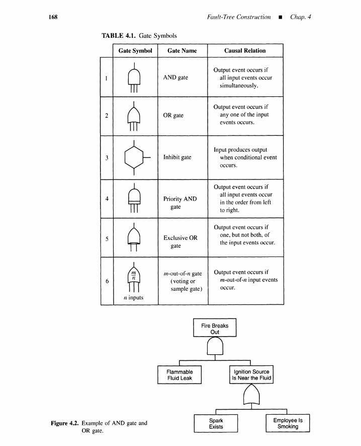
168
TABLE 4.1. Gate Symbols
Fault-Tree Construction _ Chap. 4
Gate Symbol Gate Name Causal Relation
Q Output event occurs if] AND gate all input events occur
simultaneously.
Q Output event occurs if2 OR gate anyone of the input
events occurs.
Input produces output3 Inhibit gate when conditional event
occurs.
g Output event occurs if
4 Priority ANDall input events occurin the order from left
gate to right.
QOutput event occurs if
5 Exclusive OR one, but not both, of
gate the input events occur.
~11l-out-of-n gate Output event occurs if
6n
(voting or m-out-of-n input events
sample gate) occur.
n inputs
Figure 4.2. Example of AND gate andOR gate.
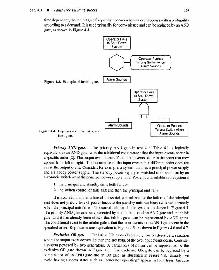
Sec. 4.3 • Fault-Tree Building Blocks 169
time dependent, the inhibit gate frequently appears when an event occurs with a probabilityaccording to a demand. It is used primarily for convenience and can be replaced by an ANDgate, as shown in Figure 4.4.
Operator Failsto Shut Down
System
Figure 4.3. Example of inhibit gate.
Figure 4.4. Expression equivalent to in-hibit gate.
Operator PushesWrong Switch when
Alarm Sounds
Operator Failsto Shut Down
System
Operator PushesWrong Switch when
Alarm Sounds
Priority AND gate. The priority AND gate in row 4 of Table 4.1 is logicallyequivalent to an AND gate, with the additional requirement that the input events occur ina specific order [2]. The output event occurs if the input events occur in the order that theyappear from left to right. The occurrence of the input events in a different order does notcause the output event. Consider, for example, a system that has a principal power supplyand a standby power supply. The standby power supply is switched into operation by anautomatic switch when the principal power supply fails. Power is unavailable in the system if
1. the principal and standby units both fail, or
2. the switch controller fails first and then the principal unit fails
It is assumed that the failure of the switch controller after the failure of the principalunit does not yield a loss of power because the standby unit has been switched correctlywhen the principal unit failed. The causal relations in the system are shown in Figure 4.5.The priority AND gate can be represented by a combination of an AND gate and an inhibitgate, and it has already been shown that inhibit gates can be represented by AND gates.The conditional event to the inhibit gate is that the input events to the AND gate occur in thespecified order. Representations equivalent to Figure 4.5 are shown in Figures 4.6 and 4.7.
Exclusive OR gate. Exclusive OR gates (Table 4.1, row 5) describe a situationwhere the output event occurs if either one, not both, of the two input events occur. Considera system powered by two generators. A partial loss of power can be represented by theexclusive OR gate shown in Figure 4.8. The exclusive OR gate can be replaced by acombination of an AND gate and an OR gate, as illustrated in Figure 4.8. Usually, weavoid having success states such as "generator operating" appear in fault trees, because
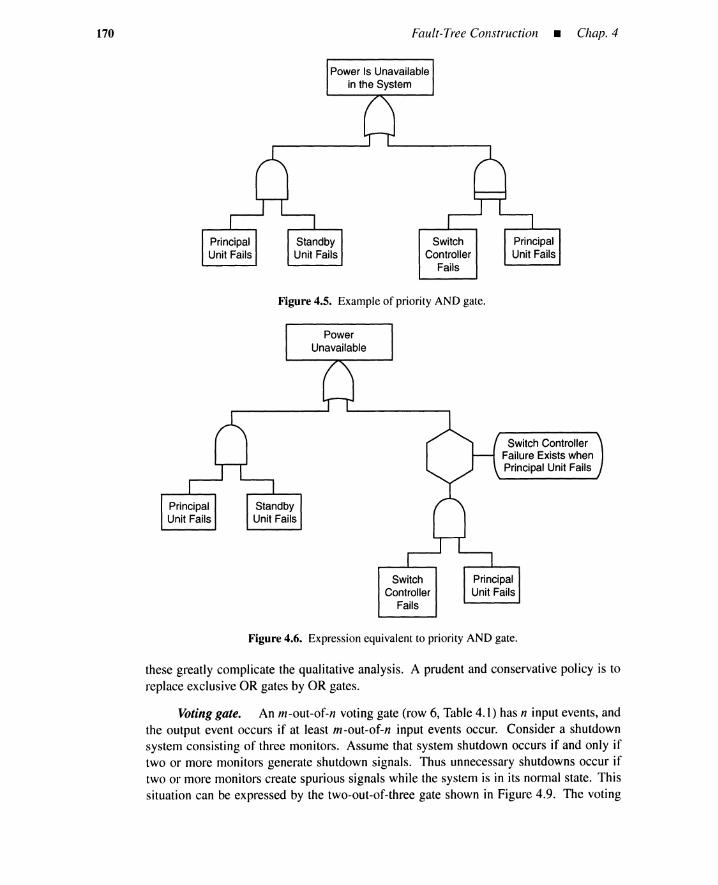
170 Fault-Tree Construction _ Chap. 4
Figure 4.5. Example of priority AND gate.
Switch ControllerFailure Exists whenPrincipal Unit Fails
Figure 4.6. Expressionequivalentto priority AND gate.
these greatly complicate the qualitative analysis. A prudent and conservative policy is toreplace exclusive OR gates by OR gates.
Voting gate. An m-out-of-n voting gate (row 6, Table 4.1) has n input events, andthe output event occurs if at least m-out-of-n input events occur. Consider a shutdownsystem consisting of three monitors. Assume that system shutdown occurs if and only iftwo or more monitors generate shutdown signals. Thus unnecessary shutdowns occur iftwo or more monitors create spurious signals while the system is in its normal state. Thissituation can be expressed by the two-out-of-three gate shown in Figure 4.9. The voting

Sec. 4.3 • Fault-Tree Building Blocks 171
PrincipalUnit Fails
StandbyUnit Fails
SwitchController
Fails
PrincipalUnit Fails
SwitchControllerFailureExistswhenPrincipal Unit Fails
Figure 4.7. Equivalent expression to priority AND gate.
Figure 4.8. Exampleof exclusiveOR gate and its equivalentexpression.
Figure 4.9. Example of two-out-of-threegate.
Monitor IGeneratesSpurious
Signal
Monitor IIGeneratesSpurious
Signal
Monitor IIIGeneratesSpurious
Signal
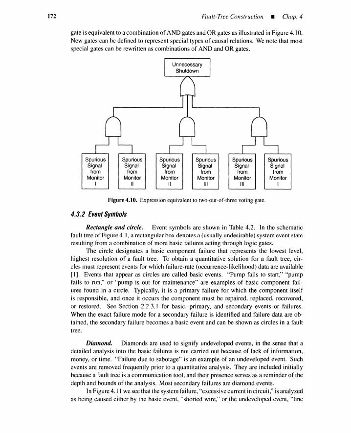
172 Fault-Tree Construction • Chap. 4
gate is equivalent to a combination of AND gates and OR gates as illustrated in Figure 4.10.New gates can be defined to represent special types of causal relations. We note that mostspecial gates can be rewritten as combinations of AND and OR gates.
Spurious Spurious Spurious Spurious Spurious SpuriousSignal Signal Signal Signal Signal Signal
from from from from from fromMonitor Monitor Monitor Monitor Monitor Monitor
I II II III III I
Figure 4.10. Expressionequivalent to two-out-of-three votinggate.
4.3.2 Event Symbols
Rectangle and circle. Event symbols are shown in Table 4.2. In the schematicfault tree of Figure 4.1, a rectangular box denotes a (usually undesirable) system event stateresulting from a combination of more basic failures acting through logic gates.
The circle designates a basic component failure that represents the lowest level,highest resolution of a fault tree. To obtain a quantitative solution for a fault tree, cir-cles must represent events for which failure-rate (occurrence-likelihood) data are available[1]. Events that appear as circles are called basic events. "Pump fails to start," "pumpfails to run," or "pump is out for maintenance" are examples of basic component fail-ures found in a circle. Typically, it is a primary failure for which the component itselfis responsible, and once it occurs the component must be repaired, replaced, recovered,or restored. See Section 2.2.3.1 for basic, primary, and secondary events or failures.When the exact failure mode for a secondary failure is identified and failure data are ob-tained, the secondary failure becomes a basic event and can be shown as circles in a faulttree.
Diamond. Diamonds are used to signify undeveloped events, in the sense that adetailed analysis into the basic failures is not carried out because of lack of information,money, or time. "Failure due to sabotage" is an example of an undeveloped event. Suchevents are removed frequently prior to a quantitative analysis. They are included initiallybecause a fault tree is a communication tool, and their presence serves as a reminder of thedepth and bounds of the analysis. Most secondary failures are diamond events.
In Figure 4.11 we see that the system failure, "excessive current in circuit," is analyzedas being caused either by the basic event, "shorted wire," or the undeveloped event, "line

Sec. 4.3 • Fault-Tree Building Blocks
TABLE 4.2. Event Symbols
Event Symbol Meaningof Symbol
6 Basic component
1 failure eventwith sufficient data
Circle
2 <> Undevelopedevent
Diamond
3 D State of system orcomponent event
Rectangle
4 CJ Conditional eventwith inhibit gate
Oval
0 House event.
5 Either occurringor not occurring
House
6 -D L Transfer symbol
Triangles
173
Figure 4.11. Example of event in dia-mond.
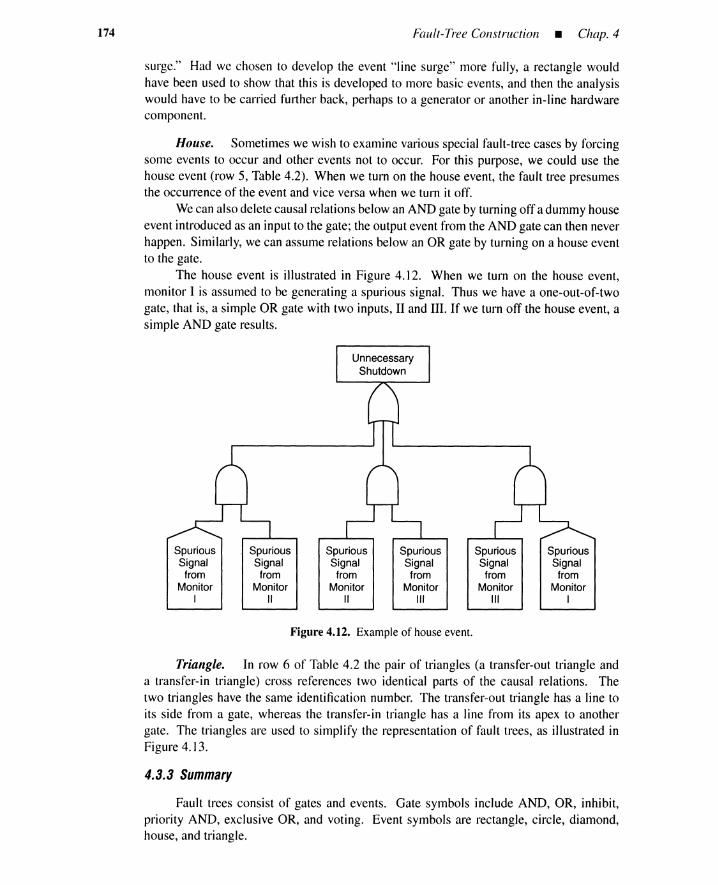
174 Fault-Tree Construction • Chap. 4
surge." Had we chosen to develop the event "line surge" more fully, a rectangle wouldhave been used to show that this is developed to more basic events, and then the analysiswould have to be carried further back, perhaps to a generator or another in-line hardwarecomponent.
House. Sometimes we wish to examine various special fault-tree cases by forcingsome events to occur and other events not to occur. For this purpose, we could use thehouse event (row 5, Table 4.2). When we turn on the house event, the fault tree presumesthe occurrence of the event and vice versa when we turn it off.
We can also delete causal relations below an AND gate by turning off a dummy houseevent introduced as an input to the gate; the output event from the AND gate can then neverhappen. Similarly, we can assume relations below an OR gate by turning on a house eventto the gate.
The house event is illustrated in Figure 4.12. When we turn on the house event,monitor I is assumed to be generating a spurious signal. Thus we have a one-out-of-twogate, that is, a simple OR gate with two inputs, II and III. If we turn off the house event, asimple AND gate results.
SpuriousSignal
fromMonitor
I
SpuriousSignal
fromMonitor
II
SpuriousSignal
fromMonitor
II
SpuriousSignalfrom
MonitorIII
SpuriousSignalfrom
MonitorIII
SpuriousSignalfrom
MonitorI
Figure 4.12. Exampleof houseevent.
Triangle. In row 6 of Table 4.2 the pair of triangles (a transfer-out triangle anda transfer-in triangle) cross references two identical parts of the causal relations. Thetwo triangles have the same identification number. The transfer-out triangle has a line toits side from a gate, whereas the transfer-in triangle has a line from its apex to anothergate. The triangles are used to simplify the representation of fault trees, as illustrated inFigure 4.13.
4.3.3 Summary
Fault trees consist of gates and events. Gate symbols include AND, OR, inhibit,priority AND, exclusive OR, and voting. Event symbols are rectangle, circle, diamond,house, and triangle.
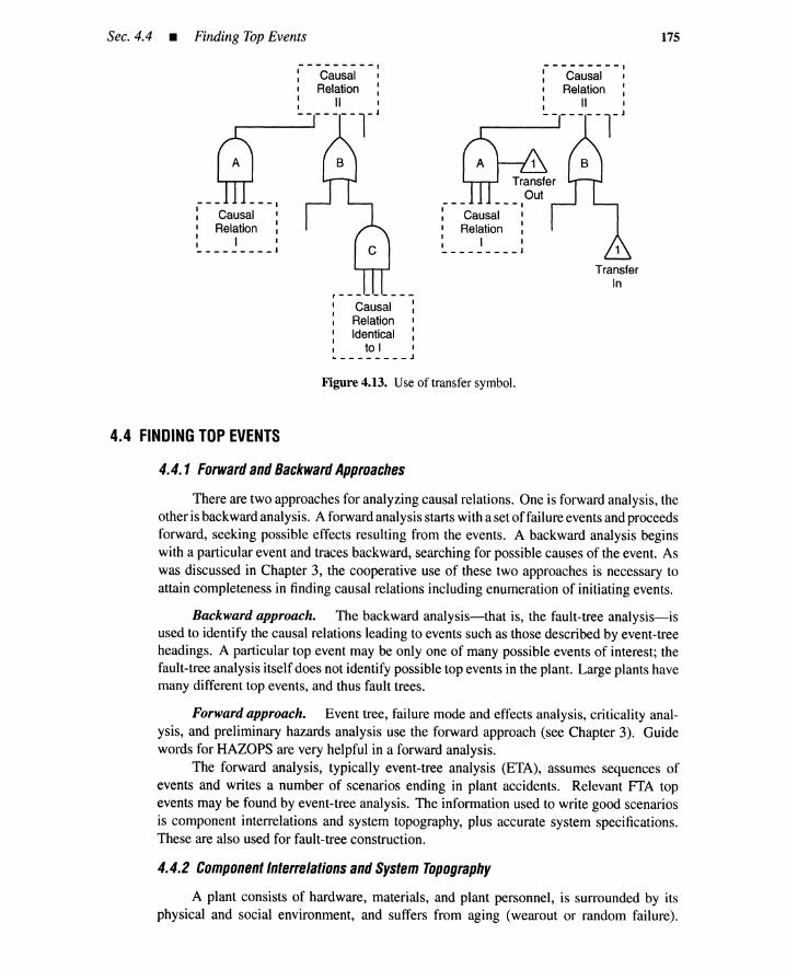
Sec. 4.4 • Finding Top Events
---------,: Causal I
• Relation :: II •____------------r I
- --.Causal •
I Relation :
: I •_________ J
r---------• Causal •• I
• Relation I
: Identical :I to I I~ J
---------,: Causal •• Relation :: II •_---------r l
TransferIn
175
Figure 4.13. Use of transfersymbol.
4.4 FINDING TOP EVENTS
4.4.1 Forward and Backward Approaches
There are two approaches for analyzing causal relations. One is forward analysis, theother is backward analysis. A forward analysis starts with a set of failure events and proceedsforward, seeking possible effects resulting from the events. A backward analysis beginswith a particular event and traces backward, searching for possible causes of the event. Aswas discussed in Chapter 3, the cooperative use of these two approaches is necessary toattain completeness in finding causal relations including enumeration of initiating events.
Backward approach. The backward analysis-that is, the fault-tree analysis-isused to identify the causal relations leading to events such as those described by event-treeheadings. A particular top event may be only one of many possible events of interest; thefault-tree analysis itself does not identify possible top events in the plant. Large plants havemany different top events, and thus fault trees.
Forward approach. Event tree, failure mode and effects analysis, criticality anal-ysis, and preliminary hazards analysis use the forward approach (see Chapter 3). Guidewords for HAZOPS are very helpful in a forward analysis.
The forward analysis, typically event-tree analysis (ETA), assumes sequences ofevents and writes a number of scenarios ending in plant accidents. Relevant FfA topevents may be found by event-tree analysis. The information used to write good scenariosis component interrelations and system topography, plus accurate system specifications.These are also used for fault-tree construction.
4.4.2 Component Interrelations and System Topography
A plant consists of hardware, materials, and plant personnel, is surrounded by itsphysical and social environment, and suffers from aging (wearout or random failure).

176 Fault-Tree Construction • Chap. 4
Accidents are caused by one or a set of physical components generating failure events.The environment, plant personnel, and aging affect the system only through the physi-cal components. Components are not necessarily the smallest constituents of the plant;they may be units or subsystems; a plant operator can be viewed as a physical compo-nent.
Each physical component in a system is related to the other components in a specificmanner, and identical components ITIay have different characteristics in different plants.Therefore, we must clarify component interrelations and system topography. The inter-relations and the topography are found by examining plant piping, electrical wiring, me-chanical couplings, information flows, and the physical location of components. Thesecan be best expressed by a plant schematic; plant word models and logic flow charts alsohelp.
4.4.3 Plant Boundary Conditions
Plant boundary. The system environment, in principle, includes the entire worldoutside the plant, so an appropriate boundary for the environment is necessary to preventthe initiating-eventand event-tree analyses from diverging. Only major,highly probable, orcritical events should be considered in the initial steps of the analysis. FMECA can be usedto identify these events. Wecan include increasingly less probable or less serious events asthe analysis proceeds, or choose to ignore them.
Initial conditions. System specification requires a careful delineation of compo-nent initial conditions. All components that have more than one operating state generateinitial conditions. For example, if the initial quantity of fluid in a tank is unspecified,the event "tank is full" is one initial condition, while "tank is empty" is another. Forthe railway in Figure 3.], the position of train B is an initial condition for the initiatingevent, "train A unscheduled departure," The time domain must also be specified; start-upor shutdown conditions, for example, can generate different accidents than a steady-stateoperation.
When enough information on the plant has been collected, we can write event-treescenarios and define fault-tree top events. Causal relations leading to each top event arethen found by fault-tree analysis. Combinations of failures (cut sets) leading to an accidentsequence are determined from these causal relations.
4.4.4 Example ofPreliminary Forward Analysis
System schematic. Consider the pumping system in Figure 4.14 [3,4]. This sche-matic gives the component relationships described by the following model:
Word model. In the start-up mode, to start the pumping, reset switch S] is closedand then immediately opened. This aIJows current to flow in the control branch circuit,activating relay coils KI and K2; relay K I contacts are closed and latched, while K2contacts close and start the pump motor.
In the shutdown mode, after approximately 20 s, the pressure switch contacts shouldopen (since excess pressure should be detected by the pressure switch), deactivating thecontrol circuit, de-energizing the K2 coil, opening the K2 contacts, and thereby shuttingthe motor off. If there is a pressure switch hang-up (emergency shutdown mode), the timer

Sec. 4.4 • Finding Top Events 177
Pressure Switch
OutletValve
II
r--------------~--II I I
I II I
ResetSwitch S1
K1 Contacts
CircuitB
- - - - - - - - - - - - - - - - - - - - _I
I
-------------~-------II
Reservoir
PressureTank
Figure 4.14. Systemschematic for a pumpingsystem.
relay contacts should open after 60 s, de-energizing the Kl coil, which in tum de-energizesthe K2 coil, shutting off the pump. We assume that the timer resets itself automaticallyafter each trial, that the pump operates as specified, and that the tank is emptied of fluidafter every run.
Sequence flow chart. We can also introduce the Figure 4.15 flow chart, showingthe sequential functioning of each component in the system with respect to each operationalmode.
Preliminary forward analysis. Forward analyses such as PHA and FMEA arecarried out, and we detect sequences of component-failure events leading to the accidents.For the pumping system of Figure 4.14:
1. Pressure switch fails to open ~ timer fails to time-out~ overpressure -+ ruptureof tank
2. Reset switch fails to open -+ pressure switch fails to open ~ overpressure ~rupture of tank
3. Reset switch fails to close -+ pump does not start ~ fluid from the tank becomesunavailable
4. Leak of flammable fluid from tank ~ relay sparks -+ fire

""""....J
QO
Tra
nsiti
onto
Pum
ping
K2
-E
nerg
ized
(Clo
sed)
T/R
-C
ont.
Clo
sed
PIS
-C
ont.
Clo
sed
Pum
p-
Sta
rts
DE
MA
ND
MO
DE
Sta
rt-u
pT
rans
ition
-P
UM
PIN
GM
OD
ET
rans
ition
toR
eady
SH
UT
DO
WN
MO
DE
~
Res
etS
witc
h-
Con
t.O
pen
Res
etR
IS-
Con
t.O
pen
K2
-D
e-en
ergi
zed
RIS
-C
ont.
Ope
nR
elay
K1
-C
ont.
Ope
nS
witc
h-
Mom
enta
rily
K1
-C
ont.
Clo
sed
(Op
en
)K
1-
Con
t.C
lose
dR
elay
K2
-C
ont.
Ope
nC
lose
dK
2-
Con
t.C
lose
dK
2-
Con
t.O
pen
Tim
erR
elay
-C
ont.
Clo
sed
T/R
-C
ont.
Clo
sed
T/R
-R
eset
sto
T/R
-C
ont.
Clo
sed
Zer
oT
ime
Pre
ssur
eS
witc
h-
Con
t.C
lose
dR
elay
and
Tim
ing
PIS
-C
ont.
Ope
nP
IS-
Con
t.O
pen
K1
-E
nerg
ized
PIS
-C
ont.
Clo
sed
Pum
p-
Sto
psan
dM
onito
ring
~an
dLa
tche
dan
dM
onito
ring
Rel
ayK
2-
Ene
rgiz
edan
dC
lose
d
Tim
erR
elay
-S
tart
sK
1-
Con
t.O
pen
Tim
ing
K2
-C
ont.
Ope
nT
/R-
Tim
esO
utan
dP
ress
ure
Mom
enta
rily
Ope
nsS
witc
h-
Mon
itorin
gPI
S-
Fai
led
Clo
sed
Pre
ssur
eP
ump
-S
tops
Em
erge
ncy
Shu
tdow
n(A
ssum
eP
ress
ure
Sw
itch
Han
gU
p)
EM
ER
GE
NC
YS
HU
TD
OW
N
RIS
-C
ont.
Ope
nK
1-
Con
t.O
pen
K2
-C
ont.
Ope
nT
/R-
Con
t.C
lose
dP
IS-
Con
t.C
lose
d
Fig
ure
4.15
.P
umpi
ngsy
stem
flow
char
t.
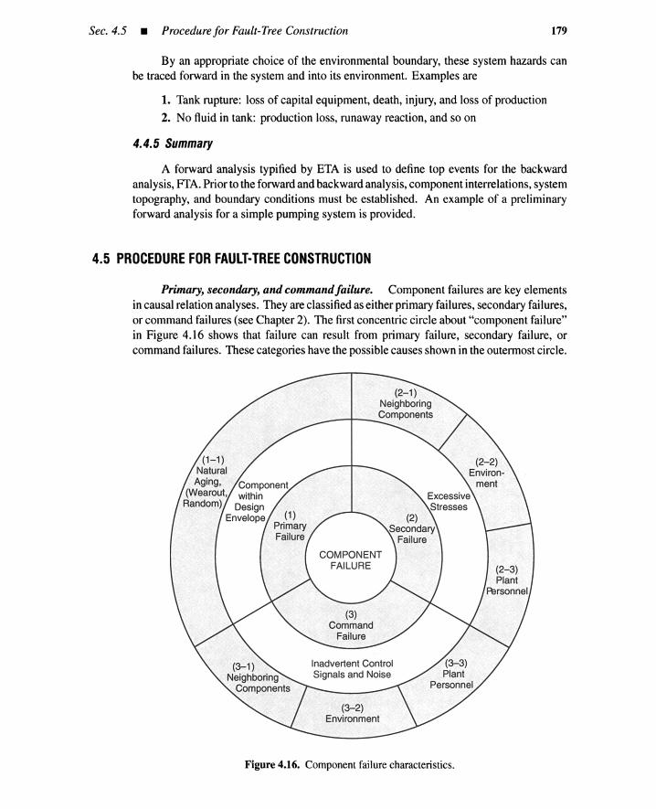
Sec. 4.5 • Procedure for Fault-Tree Construction 179
By an appropriate choice of the environmental boundary, these system hazards canbe traced forward in the system and into its environment. Examples are
1. Tank rupture: loss of capital equipment, death, injury, and loss of production
2. No fluid in tank: production loss, runaway reaction, and so on
4.4.5 Summary
A forward analysis typified by ETA is used to define top events for the backwardanalysis, FTA. Prior to the forward and backward analysis, component interrelations, systemtopography, and boundary conditions must be established. An example of a preliminaryforward analysis for a simple pumping system is provided.
4.5 PROCEDURE FOR FAULT·TREE CONSTRUCTION
Primary, secondary, and commandfailure. Component failures are key elementsin causal relation analyses. They are classified as either primary failures, secondary failures,or command failures (see Chapter 2). The first concentric circle about "component failure"in Figure 4.16 shows that failure can result from primary failure, secondary failure, orcommand failures. These categories have the possible causes shown in the outermost circle.
Figure 4.16. Component failure characteristics.
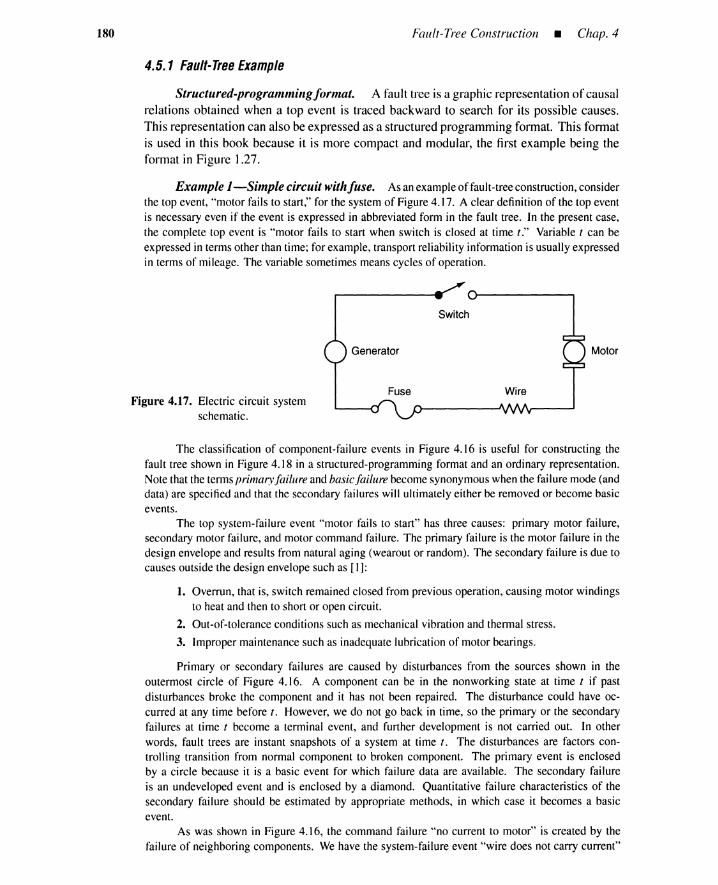
180 Fault-Tree Construction _ Chap. 4
4.5.1 Faull-Tree Example
Structured-programmingformat. A fault tree is a graphic representation of causalrelations obtained when a top event is traced backward to search for its possible causes.This representation can also be expressed as a structured programming format. This formatis used in this book because it is more compact and modular, the first example being theformat in Figure 1.27.
Example I-Simple circuit withfuse. Asan exampleof fault-treeconstruction,considerthe top event, "motor fails to start," for the system of Figure 4.17. A clear definition of the top eventis necessary even if the event is expressed in abbreviated form in the fault tree. In the present case,the complete top event is "motor fails to start when switch is closed at time t " Variable t can beexpressed in terms other than time; for example, transport reliability information is usuallyexpressedin terms of mileage. The variable sometimes means cycles of operation.
Generator
Switch
Motor
Figure 4.17. Electric circuit systemschematic.
Fuse Wire
The classification of component-failure events in Figure 4.16 is useful for constructing thefault tree shown in Figure 4.18 in a structured-programming format and an ordinary representation.Note that the termsprimary failure and basicfailure becomesynonymouswhen the failure mode (anddata) are specifiedand that the secondary failures will ultimately either be removed or become basicevents.
The top system-failure event "motor fails to start" has three causes: primary motor failure,secondary motor failure, and motor command failure. The primary failure is the motor failure in thedesign envelope and results from natural aging (wearout or random). The secondary failure is due tocauses outside the design envelope such as [I]:
1. Overrun, that is, switch remained closed from previousoperation, causing motor windingsto heat and then to short or open circuit.
2. Out-of-toleranceconditions such as mechanical vibration and thermal stress.
3. Improper maintenance such as inadequate lubricationof motor bearings.
Primary or secondary failures are caused by disturbances from the sources shown in theoutermost circle of Figure 4.16. A component can be in the nonworking state at time t if pastdisturbances broke the component and it has not been repaired. The disturbance could have oc-curred at any time before t. However, we do not go back in time, so the primary or the secondaryfailures at time t become a terminal event, and further development is not carried out. In otherwords, fault trees are instant snapshots of a system at time t. The disturbances are factors con-trolling transition from normal component to broken component. The primary event is enclosedby a circle because it is a basic event for which failure data are available. The secondary failureis an undeveloped event and is enclosed by a diamond. Quantitative failure characteristics of thesecondary failure should be estimated by appropriate methods, in which case it becomes a basicevent.
As was shown in Figure 4.16, the command failure "no current to motor" is created by thefailure of neighboring components. We have the system-failureevent "wire does not carry current"

MotorFails to Start-Primary MotorFailureSecondary MotorFailureNo Currentto Motor-Generator Doesnot SupplyCurrent-PrimaryGenerator Failure
Secondary Generator FailureCircuitDoesnot CarryCurrent-Wire~ Current-Primary Wire Failure (Open)
Secondary Wire Failure (Open)Switch Doesnot CarryCurrent-Primary Switch Failure (Open)
Secondary Switch Failure (Open)Open Fuse-Primary FuseFailure (Open)
Secondary FuseFailure (Open)
1
234
567891011
1213
1415
161718
1920212223
24
Figure 4.18. Electric circuit fault tree.
181
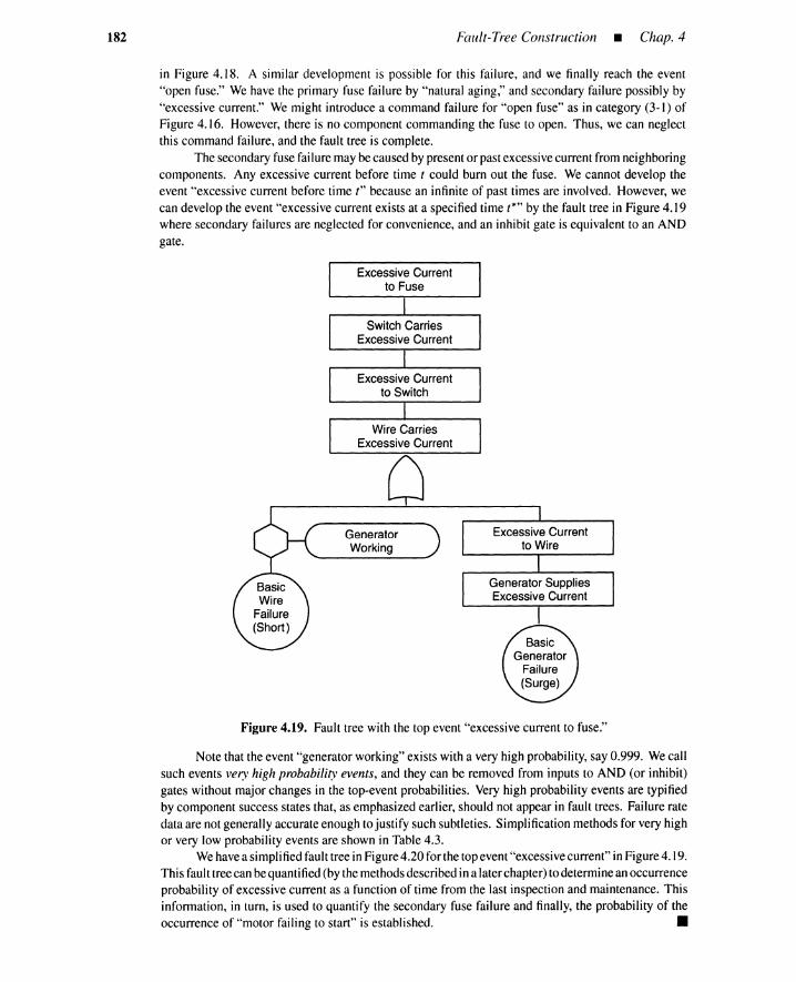
GeneratorWorking
182 Fault-Tree Construction • Chap. 4
in Figure 4.18. A similar development is possible for this failure, and we finally reach the event"open fuse." Wehave the primary fuse failure by "natural aging,"and secondary failure possiblyby"excessivecurrent." Wemight introducea command failure for "open fuse" as in category (3-1) ofFigure 4.16. However, there is no componentcommanding the fuse to open. Thus, we can neglectthis commandfailure, and the fault tree is complete.
The secondaryfusefailuremaybecausedbypresentor pastexcessive currentfromneighboringcomponents. Any excessive current before time t could burn out the fuse. Wecannot develop theevent "excessivecurrent before time t" becausean infiniteof past times are involved. However, wecan developthe event"excessivecurrent exists at a specified time t:" by the fault tree in Figure4.19where secondaryfailures are neglected for convenience, and an inhibitgate is equivalent to an ANDgate.
Figure 4.19. Fault tree with the top event "excessivecurrent to fuse."
Note that theevent"generatorworking"exists witha veryhighprobability, say 0.999. Wecallsuch events vel)' high probability events, and they can be removed from inputs to AND (or inhibit)gates without majorchanges in the top-event probabilities. Very high probability eventsare typifiedby componentsuccessstates that, as emphasizedearlier,should not appear in fault trees. Failureratedata are notgenerallyaccurateenoughtojustify such subtleties. Simplification methodsfor veryhighor very low probabilityeventsare shownin Table4.3.
Wehavea simplified faulttreeinFigure4.20for thetopevent"excessive current"inFigure4.19.Thisfaulttreecanbequantified (bythemethodsdescribedina laterchapter)todetermineanoccurrenceprobabilityof excessive current as a function of time from the last inspection and maintenance. Thisinformation, in turn, is used to quantify the secondaryfuse failure and finally, the probability of theoccurrenceof "motor failing to start" is established. •
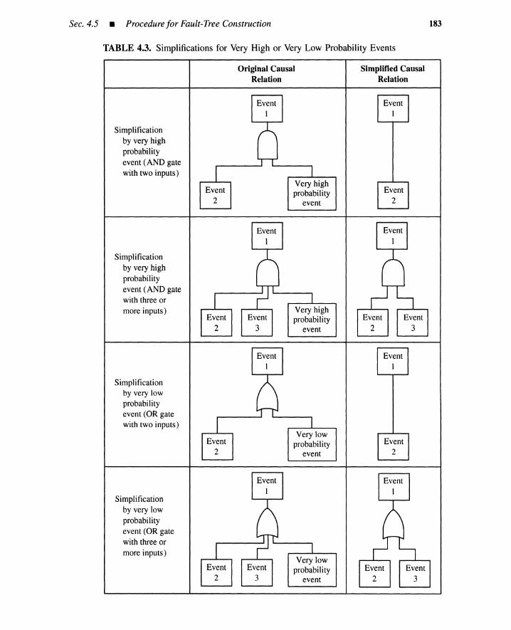
Sec. 4.5 • Procedure for Fault-Tree Construction
TABLE 4.3. Simplifications for Very High or Very Low Probability Events
183
Simplificationby very highprobabilityevent (AND gatewith two inputs)
Simplificationby very highprobabilityevent (AND gatewith three ormore inputs)
Simplificationby very lowprobabilityevent (OR gatewith two inputs)
Simplificationby very lowprobabilityevent (OR gatewith three ormore inputs)
OriginalCausalRelation
Very highprobability
event
SimplifiedCausalRelation

184 Fault-Tree Construction _ Chap. 4
ExcessiveCurrentto Fuse
Figure 4.20. Fault tree obtained by ne-glecting generator not deadevent.
4.5.2 Heuristic Guidelines
Guidelines. Heuristic guidelines for the construction of fault trees are summarizedin Table 4.4 and Figure 4.21, and given below.
1. Replace an abstract event by a less abstract event. Example: "motor operates toolong" versus "current to motor too long."
2. Classify an event into more elementary events. Example: "tank rupture" versus"rupture by overfilling" or "rupture due to runaway reaction."
3. Identify distinct causes for an event. Example: "runaway reaction" versus "largeexotherm" and "insufficient cooling."
4. Couple trigger event with "no protective action." Example: "overheating" versus"loss of cooling" coupled with "no system shutdown." Note that causal relationsof this type can be dealt with in an event tree that assumes an initiating event "lossof cooling" followed by "no system shutdown"; a single large fault tree can bedivided into two smaller ones by using event-tree headings.
5. Find cooperative causes for an event. Example: "fire" versus "leak of flammablefluid" and "relay sparks."
6. Pinpoint a component-failure event. Example: "no current to motor" versus "noCUITent in wire." Another example is "no cooling water" versus "main valve isclosed" coupled with "bypass valve is not opened."
7. Develop a component failure via Figure 4.21. As we trace backward to searchfor more basic events, we eventually encounter component failures that can bedeveloped recursively by using the Figure 4.21 structure.
State-of-component event. If an event in a rectangle can be developed in the formof Figure 4.21, Lambert calls it a state-of-component event [3]. In this case, a component tobe analyzed is explicitly specified. Otherwise, an event is called a state-of-system event. Forthe state-of-system event, we cannot specify a particular component to analyze. More thanone hardware component or subsystems are responsible for a state-of-system event. Suchevents should be developed by guidelines (1) through (6) until state-of-component eventsappear. The state-of-component events are developed further in terms of primary failures,secondary failures, and command failures. If the primary or secondary failures are notdeveloped further, they become terminal (basic) events in the fault tree under construction.The command failures are usually state-of-system failure events that are developed furtheruntil relevant state-of-component events are found. The resulting state-of-component eventsare again developed via Figure 4.21. The procedure is repeated, and the development iseventually terminated when there is no possibility of command failures.
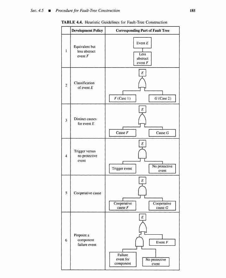
Sec. 4.5 • Procedure for Fault-Tree Construction
TABLE 4.4. Heuristic Guidelines for Fault-Tree Construction
185
2
3
4
5
6
Development Policy
Equivalentbutless abstractevent F
Classificationof event E
Distinct causesfor event E
Trigger versusno protectiveevent
Cooperative cause
Pinpoint acomponentfailure event
Corresponding Part of Fault Tree
Lessabstractevent F

186 Fault-Tree Construction _ Chap. 4
Figure 4.21. Development of a com-ponent failure (state-of-component event).
Component Failure--Primary Component Failure
Secondary Component Failure
Command Failure
Top event versus event tree. Top events are usually state-of-system failure events.Complicated top events such as "radioactivity release" and "containment failure" are de-veloped in top portions of fault trees. The top portion includes undesirable events andhazardous conditions that are the immediate causes of the top event. The top event must becarefully defined and all significant causes of the top event identified. The marriage of faultand event trees can simplify the top-event development because top events as event-treeheadings are simpler than analyzing the entire accident by a large, single fault tree. In otherwords, important aspects of the tree-top portions can be included in an event tree.
More guidelines. To our heuristic guidelines, we can add a few practical consider-ations by Lambert [3]. Note that the description about normal function is equivalent to theremoval of very high probability events from the fault tree (see Table 4.3).
Expect no miracles; if the "normal" functioning of a component helps to propagate a failuresequence, it must be assumed that the component functions "normally": assume that ignitionsources are always present. Write complete, detailed failure statements. Avoid direct gate-to-gate relationships. Think locally. Always complete the inputs to a gate. Include notes onthe side of the fault tree to explain assumptions not explicit in the failure statements. Repeatfailure statements on both sides of the transfer symbols.
Example 2-Afault tree without an event tree. This example shows how the heuristicguidelines of Table 4.4 and Figure 4.21 can be used to construct a fault tree for the pressure tanksystem in Figure 4.22. The fault tree is not based on an event tree and is thus larger in size than thosein Figure 1.10. This example also shows that the marriage of fault and event trees greatly simplifiesfault-tree construction.
A fault tree with the top event "tank rupture" is shown in Figures 4.23 and 4.24 in a structured-programming and ordinary representations, respectively. This tree shows which guidelines are usedto develop events in the tree. The operator in this example can be regarded as a system component,and the OR gate on line 23 is developed by using the guidelines of Figure 4.21 convenientlydenotedas imaginaryrow7 of Table4.4. A primaryoperator failuremeans that the operator functioningwithin

Sec. 4.5 • Procedurefor Fault-Tree Construction 187
Switch
r-- Power
Supply
Operator
Contacts
Timer
Tank
Figure 4.22. Schematic diagram for a pumping system.
1 PressureTank Rupture (Heuristic Guideline)
2 _(ROW7)3 PrimaryTank Failure: <Event 1>4 SecondaryTank Failure5 Overpressureto Tank6 Motor Operates too Long (Row 1)7 Current to Motor too Long (Row 1)8 _(ROW4)
9 Contacts Are Closed too Long
10 II1II (Row 7)
11 PrimaryContacts Failure: <Event 2>
12 SecondaryContacts Failure13 No Commandto Open Contacts14 _(ROW 7)15 PrimaryTimer Failure: <Event 3>16 SecondaryTimer Failure17 Switch Is Closed too Long18 _(ROW7)
19 Primary Switch Failure: <Event 4>
20 SecondarySwitch Failure21 No Command to Open Switch
22 Operator Does not Open Switch (Row 1)23 _(ROW7)
24 PrimaryOperator Failure: <Event 5>25 SecondaryOperator Failure
26 No Command to Operator27 _(ROW7)
28 PrimaryAlarm Failure: <Event 6>
29 Secondary Alarm Failure
Figure 4.23. Fault tree for pumping system.
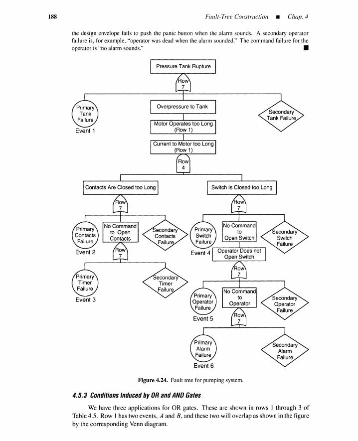
Event 1
188 Fault-Tree Construction • Chap. 4
the design envelope fails to push the panic button when the alarm sounds. A secondary operatorfailure is, for example, "operator was dead when the alarm sounded." The command failure for theoperator is "no alarm sounds." •
Event6
Figure 4.24. Fault tree for pumping system.
4.5.3 Conditions Induced byOR and AND Gates
We have three applications for OR gates. These are shown in rows I through 3 ofTable4.5. Row I has two events, A and B, and these two will overlap as shown in the figureby the corresponding Venn diagram.
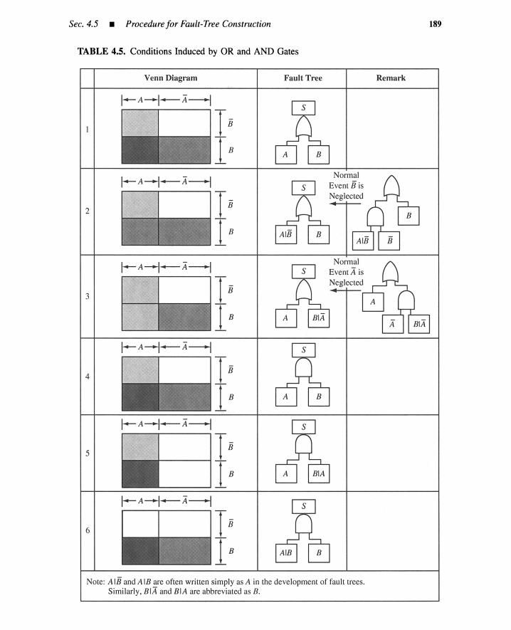
Sec. 4.5 • Procedure for Fault-Tree Construction
TABLE 4.5. Conditions Induced by OR and AND Gates
189
2
3
4
5
6
Venn Diagram Faul t Tre e
NormalEvent 8 isNeg lected
Remark
Note: A18 and A IB are often written simply as A in the deve lopment of fau lt trees.Similarly, B1 A and B1 A are abbreviated as B.
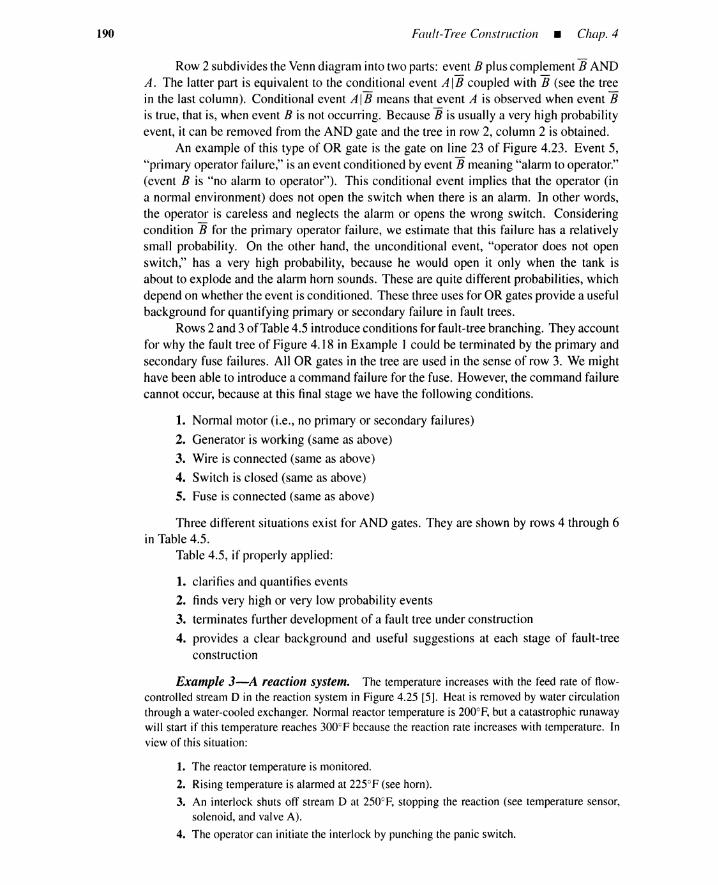
190 Fault-Tree Construction • Chap. 4
Row 2 subdivides the Venn diagram into two parts: event B plus complement BANDA. The latter part is equivalent to the conditional event A(S coupled with B (see the treein the last column). Conditional event A IB means that event A is observed when event Bis true, that is, when event B is not occurring. Because B is usually a very high probabilityevent, it can be removed from the AND gate and the tree in row 2, column 2 is obtained.
An example of this type of OR gate is the gate on line 23 of Figure 4.23. Event 5,"primary operator failure," is an event conditioned by event B meaning "alarm to operator."(event B is "no alarm to operator"). This conditional event implies that the operator (ina normal environment) does not open the switch when there is an alarm. In other words,the operator is careless and neglects the alarm or opens the wrong switch. Consideringcondition B for the primary operator failure, we estimate that this failure has a relativelysmall probability. On the other hand, the unconditional event, "operator does not openswitch," has a very high probability, because he would open it only when the tank isabout to explode and the alarm horn sounds. These are quite different probabilities, whichdepend on whether the event is conditioned. These three uses for OR gates provide a usefulbackground for quantifying primary or secondary failure in fault trees.
Rows 2 and 3 of Table 4.5 introduce conditions for fault-tree branching. They accountfor why the fault tree of Figure 4. ]8 in Example ] could be terminated by the primary andsecondary fuse failures. All OR gates in the tree are used in the sense of row 3. We mighthave been able to introduce a command failure for the fuse. However, the command failurecannot occur, because at this final stage we have the following conditions.
1. Normal motor (i.e., no primary or secondary failures)
2. Generator is working (same as above)
3. Wire is connected (same as above)
4. Switch is closed (same as above)
5. Fuse is connected (same as above)
Three different situations exist for AND gates. They are shown by rows 4 through 6in Table 4.5.
Table 4.5, if properly applied:
1. clarifies and quantifies events
2. finds very high or very low probability events
3. terminates further development of a fault tree under construction
4. provides a clear background and useful suggestions at each stage of fault-treeconstruction
Example 3-A reaction system. The temperature increases with the feed rate of flow-controlled stream 0 in the reaction system in Figure 4.25 [5]. Heat is removed by water circulationthrough a water-cooled exchanger. Normal reactor temperatureis 200°F, but a catastrophic runawaywill start if this temperature reaches 300cF because the reaction rate increases with temperature. Inviewof this situation:
I. The reactor temperatureis monitored.
2. Rising temperatureis alarmed at 225°F (see horn).
3. An interlock shuts off stream D at 250cF, stopping the reaction (see temperature sensor,solenoid, and valve A).
4. The operator can initiate the interlock by punching the panic switch.
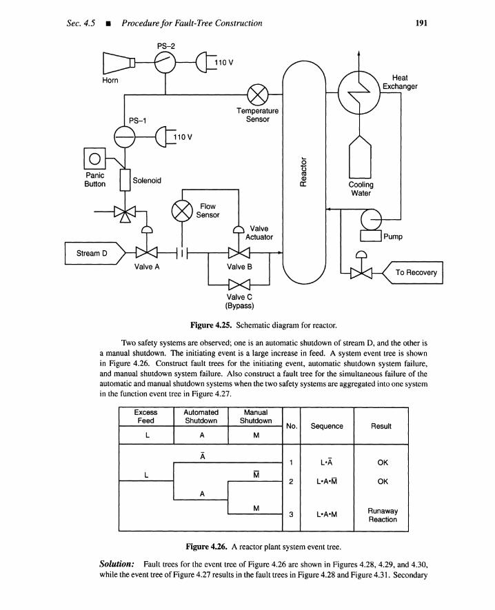
Sec.4.5 • Procedure for Fault-Tree Construction 191
PS-2
To Recovery
Pump
CoolingWater
'-ot5ttSQ)
CI:
ValveActuator
TemperatureSensorPS-1
Stream D
Valve C(Bypass)
Figure 4.25. Schematic diagram for reactor.
Two safety systems are observed; one is an automatic shutdown of stream D, and the other isa manual shutdown. The initiating event is a large increase in feed. A system event tree is shownin Figure 4.26. Construct fault trees for the initiating event, automatic shutdown system failure,and manual shutdown system failure. Also construct a fault tree for the simultaneous failure of theautomatic and manual shutdown systems when the two safety systems are aggregated into one systemin the function event tree in Figure 4.27.
Excess Automated ManualFeed Shutdown Shutdown
No. Sequence ResultL A M
AL*A1 OK
L ML*A*M2 OK
A
M Runaway3 L*A*MReaction
Figure 4.26. A reactor plant system event tree.
Solution: Fault trees for the event tree of Figure 4.26 are shown in Figures 4.28, 4.29, and 4.30,while the event tree of Figure 4.27 results in the fault trees in Figure 4.28 and Figure 4.31. Secondary
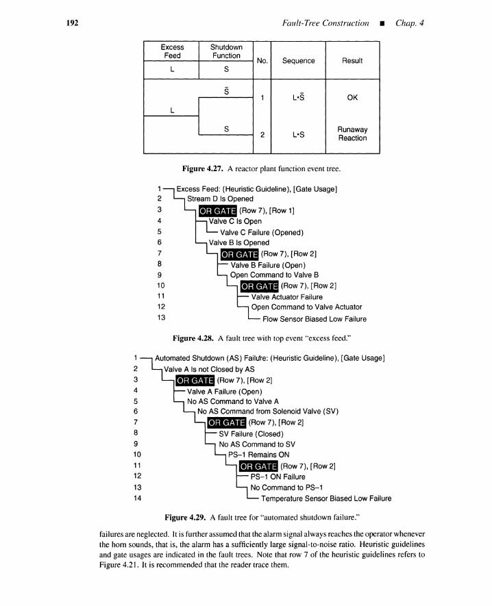
192 Fault-Tree Construction _ Chap. 4
Excess ShutdownFeed Function
No. Sequence ResultL S
SL*S1 OK
L
SL*S
Runaway2 Reaction
Figure 4.27. A reactor plant function event tree.
1 Excess Feed: (Heuristic Guideline), [Gate Usage]2 Stream D Is Opened
3 _ (Row 7), [Row 1]
4 Valve C Is Open
5 Valve C Failure (Opened)
6 Valve B Is Opened
7 __(Row 7), [Row 2]
8 Valve B Failure (Open)9 Open Command to Valve B
10 &DIll! (Row 7), [Row 2]
11 Valve Actuator Failure
12 Open Command to Valve Actuator
13 Flow Sensor Biased Low Failure
Figure 4.28. A fault tree with top event "excess feed."
1
2
34
56
7
8
9
10
11
12
13
14
Figure 4.29. A fault tree for "automated shutdown failure."
failuresare neglected. It is furtherassumed that thealarm signalalwaysreaches theoperator wheneverthe hom sounds, that is, the alarm has a sufficiently large signal-to-noise ratio. Heuristic guidelinesand gate usages are indicated in the fault trees. Note that row 7 of the heuristic guidelines refers toFigure 4.21. It is recommended that the reader trace them.

Sec. 4.5 • Procedurefor Fault-Tree Construction
1
2
34
5
678
9
10
1112
13
14
15
16
17
18
19
20
21
22
2324
Figure 4.30. A fault tree for "manual shutdown failure."
193
One might think that event "valve A is open" on line 4 of Figure 4.29 is a very high probabilityevent because the valve is open if the system is in normal operation. This is not true, because this openvalve is conditioned by the initiating event of the event tree in Figure 4.26. Under this circumstance,the shutdown system will operate, and "valve A is open" has a small probability of occurrence. Thisevent can be regarded as an input to an AND gate in accident sequence L*A*M in Figure 4.26, andshould not be neglected.
We note that a single large fault tree without an event tree is given in our previous text [6,7].In this fault tree, AND gates appear to show that the plant is designed so as to protect it from asingle failure event, that is, an initiating event in this case. The fault trees in Figures 4.28 to 4.30have no AND gate because protection features have been included in headings of the system eventtree. The fault tree in Figure 4.31 has an AND gate because this represents simultaneous failuresof automatic and manual shutdown features. The reaction system may have another initiating event,"loss of coolant," for which event trees and fault trees should be constructed in a similar way. •
Example 4-A pressure tank system. Consider the pressure tank system shown in Fig-ure 4.14. This system has been a bit of a straw-man since it was first published by Vesely in 1971[8]. It appears also in Barlow and Proschan [9]. A single large fault tree is given in our previoustext [6,7] and shown as Figure 4.32. It is identical to that given by Lambert [3] except for someminor modifications. The fault tree can be constructed by the heuristic guidelines of Table 4.4. Itdemonstrates the gate usages of Table 4.5.
We now show other fault trees for this system constructed by starting with event trees. Theplant in Figure 4.14 is similar to the plant in Figure 4.22. A marriage of event and fault trees considersas an initiating event, "pump overrun." Because the plant of Figure 4.14 has neither an operator nor arelief valve as safety systems, a relatively large fault tree for the initiating event would be constructed,
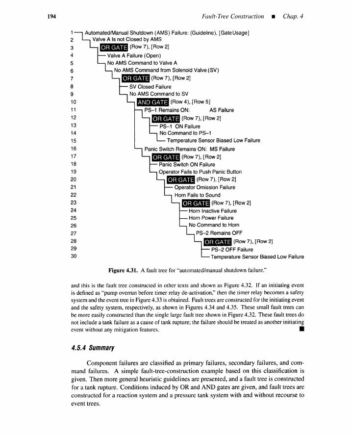
194 Fault-Tree Construction _ Chap. 4
1 Automated/Manual Shutdown(AMS) Failure: (Guideline), [GateUsage]2 Valve A Is not Closed by AMS3 &II1II (Row 7), [Row 2]
4 Valve A Failure (Open)5 No AMS Commandto Valve A6 No AMS Commandfrom SolenoidValve(SV)
7 11&1(Row 7), [Row 2]
8 SV Closed Failure9 No AMS Commandto SV
10 _(RoW4),[ROW5]
11 PS-1 RemainsON: AS Failure
12 IiDii (Row 7), [Row 2]
13 PS-1 ON Failure14 No Commandto PS-115 Temperature Sensor Biased Low Failure
16 Panic Switch RemainsON: MS Failure17 11&1 (Row 7), [Row 2]18 Panic SwitchON Failure19 Operator Fails to Push Panic Button20 &II1II (Row 7), [Row 2]
21 OperatorOmission Failure22 Horn Fails to Sound23 _ (Row 7), [Row 2]
24 Horn InactiveFailure25 Horn Power Failure26 No Command to Horn
27 PS-2 RemainsOFF
28 _ (Row 7), [Row 2]
29 PS-2 OFF Failure30 Temperature Sensor BiasedLow Failure
Figure 4.31. A fault tree for "automated/manual shutdownfailure."
and this is the fault tree constructed in other texts and shown as Figure 4.32. If an initiating eventis defined as "pump overrun before timer relay de-activation," then the timer relay becomes a safetysystemand the event tree in Figure4.33 is obtained. Fault treesare constructedfor the initiatingeventand the safety system, respectively, as shown in Figures 4.34 and 4.35. These small fault trees canbe more easily constructed than the single large fault tree shown in Figure 4.32. These fault trees donot include a tank failure as a cause of tank rupture; the failure should be treated as another initiatingevent without any mitigationfeatures. •
4.5.4 Summary
Component failures are classified as primary failures, secondary failures, and com-mand failures. A simple fault-tree-construction example based on this classification isgiven. Then more general heuristic guidelines are presented, and a fault tree is constructedfor a tank rupture. Conditions induced by OR and AND gates are given, and fault trees areconstructed for a reaction system and a pressure tank system with and without recourse toevent trees.

Sec. 4.5 • Procedurefor Fault-Tree Construction 195
Pressure Tank Rupture(Heuristic Guideline), [Usage of Gate]
_ (Row 7), [Row 3]
Primary Tank Failure
Secondary Tank Failure
Excessive Pressure to TankPump Operates too Long (Row 1)
K2 Relay Contacts Are Closed Too Long
&1&11 (Row 7), [Row 3]
K2 Relay Contacts Primary Failure
K2 Relay Contacts Secondary Failure
Current to K2 Relay Coil too Long_ (Row 4), [Row 5]
Pressure Switch (PIS) Contacts Are Closed too Long_ (Row 7), [Row 3]
Primary PIS FailureSecondary PIS Failure
Circuit B Carries Current too Long
&1&1 (Row 2 or 3), [Row 1]
Switch S1 Is Closedliliiii (Row 3 or 7), [Row 1]
Primary S1 Failure
Secondary S1 FailureK1 Relay Contacts Are Closed too Long
1&11 (Row 7), [Row 3]
K1 Relay Contacts Primary Failure
K1 Relay Contacts Secondary FailureCurrent to K1 Relay Coil too Long
Timer Relay (T/R) Contacts Are Closed too Long (Row 1)
&1&1 (Row 7), [Row 3]
Primary TIR Contacts Failure
Secondary TIR Contacts FailureCurrent to TIR Coil too Long
TIR Does not Time Out (Row 1)
12
34
567
89
10
11
12
13
14
15
16
1718
19
2021
22
23242526
27
2829
30
31
323334
Figure 4.32. A single, large fault tree for pressure tank system.
Pump TimerOverrun Relay
Number Sequence ResultPO TM
TMPO*TM1 OK
PO
TM2 PO*TM
TankRupture
Figure 4.33. Event tree for pressure tank system.

196 Fault-Tree Construction _ Chap. 4
Figure 4.34. Fault tree for "pump over-run due to pressure switchfailure."
1 Pump Overrun Is Not Arrested by Timer Relay (T/R)2 (Heuristic Guideline), [Gate Usage]3 T/R Fails to Stop Pump (Row 1)4 T/R Fails to Disconnect Circuit B (Row 1)5 _
6 Switch S1 Is Closed7 _ (Row 2 or Row 3), [Row 1]
8 Primary S1 Failure9 Secondary S1 Failure
10K1 Relay Contacts Are Closed too Long11 _ (Row 7), [Row 3]
12 K1 Relay Contacts Primary Failure
13 K1 Relay Contacts Secondary Failure
14 Current to K1 Relay Coil too Long
15 Timer Relay (T/R) Contacts Are Closed too Long (Row 1)16 &l1li (Row 7), [Row 3]
17 Primary T/R Contacts Failure18 Secondary T/R Contacts Failure19 Current to T/R Coil too Long
20 T/R Does not Time Out (Row 1)
Figure 4.35. Fault tree for "pump overrun is not arrested by timer relay."
4.6 AUTOMATED FAULT-TREE SYNTHESIS
4.6.1 Introduction
Manual generation of fault trees is a tedious, time-consuming and error-prone task.To create an FT, the system must be modeled by a suitable representation method, becauseno FT-generation method can extract more information than that contained in the model. AnFT expert would use heuristics to locally analyze an upper-level event in terms of lower-levelevents. The expert also has a global procedural framework for a systematic application ofheuristics to generate, truncate, and decompose FTs. A practical, automated FT-generationapproach requires three elements: I) a system representation, 2) expert heuristics, and 3) aprocedural framework for guiding the generation. This section describes a new automatedgeneration method based on a semantic network representation of the system to be analyzed,a rule-based event development, and a recursive three-value procedure with normal- andimpossible-event truncations and modular FT decompositions.
Automated FT-generation methods have been proposed and reviewed in Andrewsand Brennan [10], Chang et al. [11,12] and in a series of papers by Kelly and Lees [13],Mullhi et al. [14], and Hunt et al. [15]. Some of the earliest works include Fussell [16],

Sec. 4.6 • Automated Fault-Tree Synthesis 197
Salem, Apostolakis, and Okrent [17], and Henley and Kumamoto [18] . None of the methodsproposed to date is in general use.
4.6.2 System Representation bySemantic Networks
4.6.2.1 Flows.
Flow andevent propagation. A flow is defined as any material, information, energy,activity, or phenomenon that can move or propagate through the system. A system can beviewed as a pipeline structure of flows and pieces of equipment along flow paths. A varietyof flows travel the flow paths and cause events specific to the system. Typical flows are
1. material flow; liquid, gas, steam
2. information flow; signal, data, command, alarm
3. energy flow; light, heat, sound, vibration
4. activity and phenomenon; manual operation, fire, spark, high pressure
Light as a flow is generated when an electric flow is supplied to a bulb. Activities andphenomena are regarded as flows because they propagate through the system to cause events.
Flow rate, generation rate, and aperture. We focus mainly on the three attributesof a flow: flow rate, generation rate, and aperture. The aperture and generation rate aredetermined by plant equipment in the flow path. The flow rate is determined from apertureand generation rate.
The flow aperture is defined similarly to a valve; an open valve corresponds to an onswitch, whereas a closed valve corresponds to an off switch. The flow aperture is closed if,for instance, one or more valve apertures in series are closed, or at least one switch in seriesis off. The generation rate is a potential. The potential causes the positive flow rate whenthe aperture is open. The positive flow rate implies existence of a flow, and a zero flow rateimplies a nonexistence.
Flow rate, generation rate, and aperture values. Aperture attribute values areFully.Closed (F_CI), Increase (Inc), Constant (Cons), Decrease (Dec), Fully.Open (F_Op),Open, and Not.Fully .Open (Not.F.Op), The values Inc, Cons, and Dec, respectively, meanthat the aperture increases, remains constant, and decreases between F_CI (excluded) andF_Op (excluded), as shown in Figure 4.36. In a digital representation, only two attributevalues are considered, that is, F_CI and F.Op.
0F_Op
Q)
:;1:::Q) Inc Decc.«
01---------.Figure 4.36. Five aperture values. Time

198 Fault- Tree Construction • Chap. 4
In Table 4.6 aperture values are shown in column A. Attribute values Open andN_F_Op are composite, while values F_CI, Inc, Cons, Dec, and F_Op are basic.
TABLE 4.6. Flow Rate as a Function of Aperture and Generation Rate
Positive
+A_ Zero Inc Cons Dec Max
0.. F_CL Zero Zero Zero Zero Zero0l:I.' Inc Zero Inc Inc Inc, Dec Inc
~I Cons Zero Inc Cons Dec Cons c::(1)
0 0..Z Dec Zero Inc, Dec Dec Dec Dec 0F_Op Zero Inc Cons Dec Max
Not_Max
Generation Rate
As shown in row A of Table 4.6, the generation rate has attribute values Zero, Inc,Cons, Dec, Max, Positive, and Not.Max, The first five values are basic, while the last twoare composite. The flow rate has the same set of attribute values as the generation rate. SeeTable 4.6 where each cell denotes a flow rate value.
Relations between aperture, generation rate, and flow rate. The three attributesare not independent of each other. The flow rate of a flow becomes zero if its aperture isclosed or its generation rate is zero. For instance, the flow rate of electricity through a bulbis zero if the bulb has a filament failure or the battery is dead.
The flow rate is determined when the aperture and the generation rate are specified.Table 4.6 shows the relationship. Each row has a fixed aperture value, which is denoted incolumn A, and each column has a fixed generation rate value denoted in row A. Each cellis a flow rate value. The flow rate is Zero when the aperture is F.Cl or the generation rate isZero. The flow rate is not uniquely determined when the aperture is Inc and the generationrate is Dec. A similar case occurs for the Dec aperture and the Inc generation rate. In thesetwo cases, the flow rate is either Inc or Dec; we exclude the rare chance of the flow ratebecoming Cons. The two opposing combinations of aperture and generation rate in Table4.6 become causes of the flow rate being Inc (or Dec).
Relations between flow apertures and equipment apertures. Table 4.7 shows therelationships between flow apertures and equipment apertures, when equipment 1 and 2are in series along the flow path. Each column has the fixed aperture value of equipment1, and each row has the fixed aperture value of equipment 2. Each cell denotes a flow-aperture value. The flow aperture is either Inc or Dec when one equipment aperture is Incand the other is Dec. Tables 4.6 and 4.7 will be used in Section 4.6.3.3 to derive a set ofevent-development rules that search for causes of events related to the flow rate.
Flow triple event. A flow triple is defined as a particular combination (flow, at-tribute, value). For example, (electricity, flow rate, Zero) means that electricity does notexist.

Sec. 4.6 • Automated Fault-Tree Synthesis
TABLE 4.7. Flow Aperture as Function of Equipment Apertures in Series
199
Open
~ A---+- F_CI Inc Cons Dec F_Op
c, F_CI F_CI F_CI F_CI F_CI F_CI0
I Inc F_CI Inc Inc Inc, Dec Incu,~I Cons F_CI Inc Cons Dec Cons =0 (l)
c,Z Dec F_CI Inc, Dec Dec Dec Dec 0
F_Op F_CI Inc Cons Dec F_Op
Not_F_Op
Aperture 1
4.6.2.2 Basic equipment library. Equipment that controls an aperture or generationrate is catalogued in Figures 4.37 and 4.38 where a fragment of a semantic network isassociated with each piece (second column). Examples are given in the third column. Acircle represents a flow node, while a box, hexagon, or gate is an equipment node. A labeledarrow between flow and equipment node represents a relationship between the flow and theequipment. The effect to cause (backward) direction essential to fault-tree construction isrepresented by the arrow.
(A) Aperture controller. Two types of equipment, those with and those withoutcommand modes, are used for aperture control. Equipment 1 and 3 in Figure 4.37 aredevices without command. Flow F2 to equipment 2,4, 5, and 6 is the command. Equipment1 through 5 are digital devices with only two aperture values, F_CI or F.Op, while equipment6 is an analog device.
Aperture Controller without Command
1. Normally Closed Equipment (NCE): This is digital equipment that is normallyclosed (F_CI). It has no command mode and its F.Op state is caused by failureof the NCE itself. Examples include normally closed valve, normally off switch,plug, insulator, and oil barrier.
In the NCE semantic network, symbol F1 denotes a flow that is stopped bythe NCE. The vertical black stripe in the NCE box indicates a normally closedstate. The arrow labeled NCE points to the equipment that closes the F1 aperture.Suppose that the F1 flow aperture is Open. This can be traced back to an Openfailure of the NCE box.
2. Normally Open Equipment (NOE): This is digital equipment that is normallyopen (F_Op), a dual of NCE. Examples include normally open valve, normally onswitch, pipe, and electric wire.
Aperture Controller with Command. Some types of equipment can be com-manded to undergo an aperture change.
1. Closed to Open Equipment (COE): Normally this equipment is in an F_CI state.When a transition from an F_CI to an F.Op state occurs because of a command,
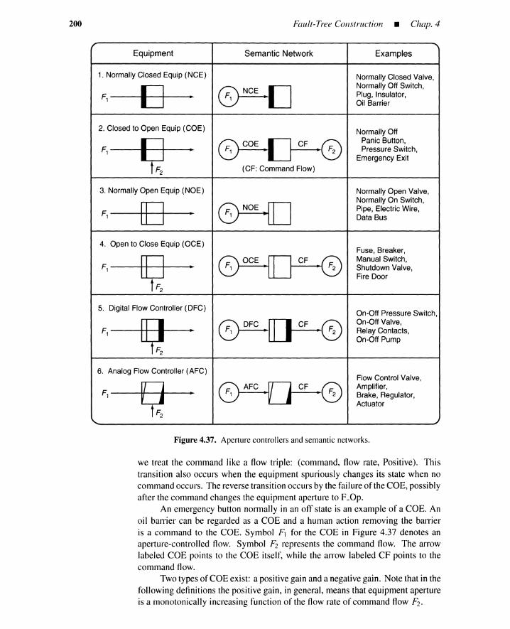
200 Fault- Tree Construction • Chap. 4
Equipment Semantic Network Examples
1. Normally Closed Equip (NCE) Normally Closed Valve,
B ~Normally Off Switch,
F1Plug, Insulator,Oil Barrier
2. Closed to Open Equip (COE) Normally Off
~Panic Button,
F1 Pressure Switch,Emergency Exit
(CF: Command Flow)
3. Normally Open Equip (NOE) Normally Open Valve,
tB ~Normally On Switch,
F1Pipe, Electric Wire,Data Bus
4. Open to Close Equip (OCE)Fuse, Breaker,
tB Manual Switch,F1 Shutdown Valve,
tF2
Fire Door
5. Digital Flow Controller (DFC)On-Off Pressure Switch,
~ ~On-Off Valve,
F1 Relay Contacts,On-Off Pump
6. Analog Flow Controller (AFC)Flow Control Valve,Amplifier,Brake, Regulator,Actuator
Figure 4.37. Aperturecontrollersand semanticnetworks.
we treat the command like a flow triple: (command, flow rate, Positive). Thistransition also occurs when the equipment spuriously changes its state when nocommand occurs. The reverse transition occurs by the failureof the COE, possiblyafter the command changes the equipment aperture to F.Op.
An emergency button normally in an off state is an example of a COE. Anoil barrier can be regarded as a COE and a human action removing the barrieris a command to the COE. Symbol F1 for the COE in Figure 4.37 denotes anaperture-controlled flow. Symbol F2 represents the command flow. The arrowlabeled COE points to the COE itself, while the arrow labeled CF points to thecommand flow.
Twotypes of COE exist: a positivegain and a negativegain. Note that in thefollowing definitions the positive gain, in general, means that equipment apertureis a monotonically increasing function of the flow rate of command flow F2•
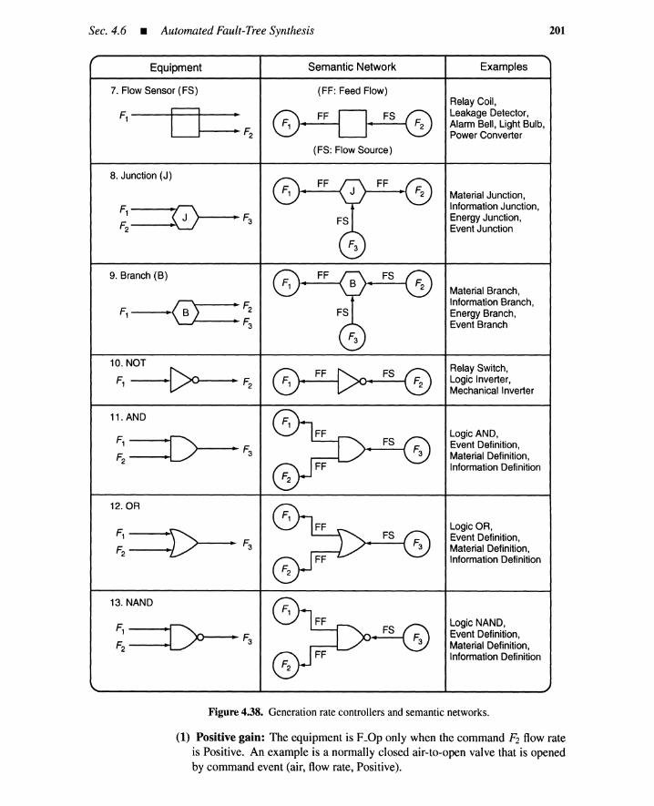
Sec. 4.6 • Automated Fault-Tree Synthesis 201
Equipment Semantic Network Examples
7. Flow Sensor (FS) (FF: Feed Flow)Relay Coil,Leakage Detector,Alarm Bell, Light Bulb,Power Converter
(FS: Flow Source)
Material Junction,Information Junction,Energy Junction,Event Junction
8. Junction (J)
9. Branch (B)
Material Branch,
·0 :F2Information Branch,
F1 Energy Branch,F3 Event Branch
10. NOT
.[>0 Relay Switch,F1
II F2Logic Inverter,Mechanical Inverter
11. AND
F1 :DLogic AND,
II F3
Event Definition,F2
Material Definition,Information Definition
12. OR
F1 :1>Logic OR,
II F3Event Definition,
F2Material Definition,Information Definition
13. NAND
F1 :[>-F3
Logic NAND,Event Definition,
F2 Material Definition,Information Definition
Figure 4.38. Generation rate controllers and semantic networks.
(1) Positive gain: The equipment is F.Op only when the command F2 flow rateis Positive. An example is a normally closed air-to-open valve that is openedby command event (air, flow rate, Positive).
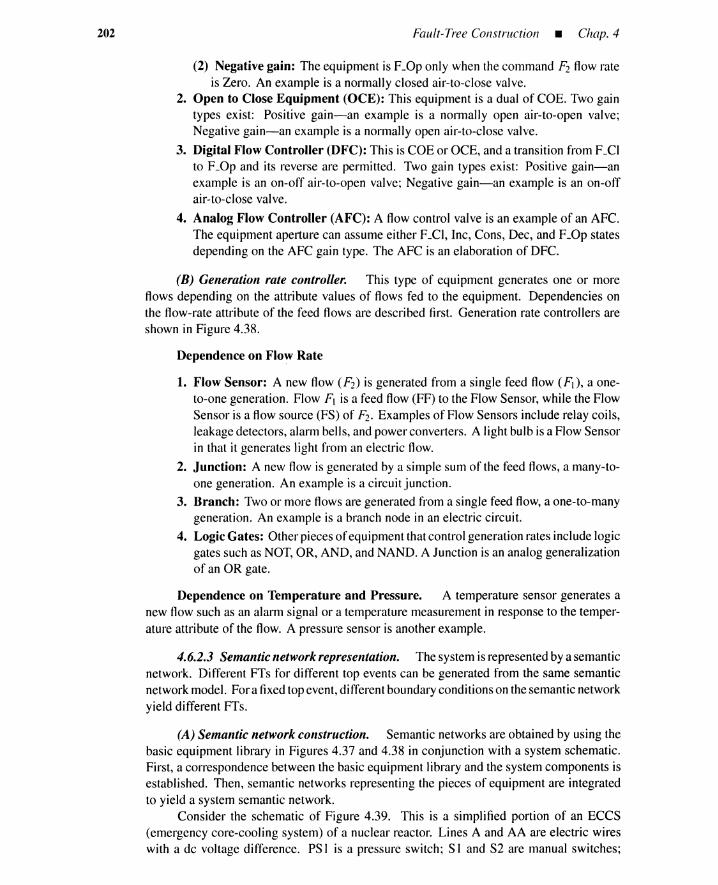
202 Fault-Tree Construction • Chap. 4
(2) Negative gain: The equipment is F_Oponly when the command F2 flowrateis Zero. An example is a normally closed air-to-close valve.
2. Open to Close Equipment (OCE): This equipment is a dual of COE. Two gaintypes exist: Positive gain-an example is a normally open air-to-open valve;Negative gain-an example is a normally open air-to-close valve.
3. Digital Flow Controller (DFC): This is COE or OCE, and a transition from F_CIto F_Op and its reverse are permitted. Two gain types exist: Positive gain-anexample is an on-off air-to-open valve; Negative gain-an example is an on-offair-to-close valve.
4. Analog Flow Controller (AFC): A flowcontrol valve is an example of an AFC.The equipment aperture can assume either F_CI, Inc, Cons, Dec, and F_Opstatesdepending on the AFC gain type. The AFC is an elaboration of DFC.
(B) Generation rate controller. This type of equipment generates one or moreflows depending on the attribute values of flows fed to the equipment. Dependencies onthe flow-rate attribute of the feed flows are described first. Generation rate controllers areshown in Figure 4.38.
Dependence on Flow Rate
1. Flow Sensor: A new flow (F2) is generated from a single feed flow (F1) , a one-to-one generation. Flow F1 is a feed flow (FF) to the Flow Sensor, while the FlowSensor is a flow source (FS) of F2. Examples of Flow Sensors include relay coils,leakage detectors, alarm bells, and power converters. A light bulb is a Flow Sensorin that it generates light from an electric flow.
2. Junction: A new flow is generated by a simple sum of the feed flows, a many-to-one generation. An example is a circuit junction.
3. Branch: Twoor more flows are generated from a single feed flow, a one-to-manygeneration. An example is a branch node in an electric circuit.
4. Logic Gates: Other pieces of equipment thatcontrol generation rates include logicgates such as NOT, OR, AND, and NAND. A Junction is an analog generalizationof an OR gate.
Dependence on Temperature and Pressure. A temperature sensor generates anew flow such as an alarm signal or a temperature measurement in response to the temper-ature attribute of the flow. A pressure sensor is another example.
4.6.2.3 Semantic network representation. The system is representedby a semanticnetwork. Different FTs for different top events can be generated from the same semanticnetwork model. Fora fixedtopevent,differentboundaryconditionson thesemantic networkyield different FTs.
(A) Semantic network construction. Semantic networks are obtained by using thebasic equipment library in Figures 4.37 and 4.38 in conjunction with a system schematic.First, a correspondence between the basic equipment library and the system components isestablished. Then, semantic networks representing the pieces of equipment are integratedto yield a system semantic network.
Consider the schematic of Figure 4.39. This is a simplified portion of an ECCS(emergency core-cooling system) of a nuclear reactor. Lines A and AA are electric wireswith a de voltage difference. PSI is a pressure switch; S I and S2 are manual switches;
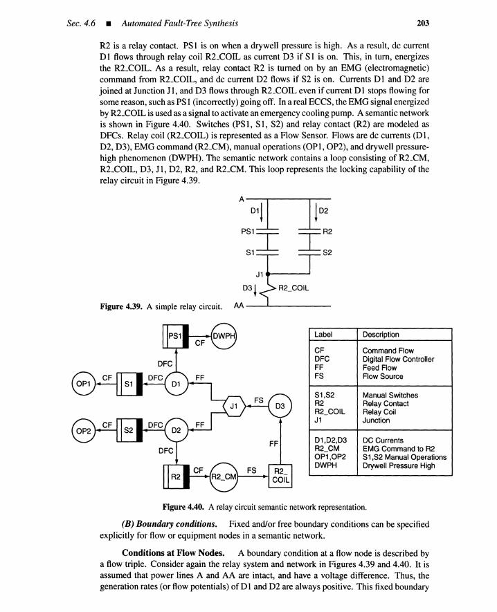
Sec.4.6 • Automated Fault-Tree Synthesis 203
R2 is a relay contact. PS 1 is on when a drywell pressure is high. As a result, de currentD1 flows through relay coil R2_COIL as current D3 if S1 is on. This, in tum, energizesthe R2_COIL. As a result, relay contact R2 is turned on by an EMG (electromagnetic)command from R2_COIL, and de current D2 flows if S2 is on. Currents DI and D2 arejoined at Junction Jl , and D3 flows through R2_COIL even if current Dl stops flowing forsome reason, such as PS 1 (incorrectly) going off. In a real ECCS, the EMG signal energizedby R2_COIL is used as a signal to activate an emergency cooling pump. A semantic networkis shown in Figure 4.40. Switches (PS1, S l , S2) and relay contact (R2) are modeled asDFCs. Relay coil (R2_COIL) is represented as a Flow Sensor. Flows are de currents (D1,D2, D3), EMG command (R2_CM), manual operations (OPl, OP2), and drywell pressure-high phenomenon (DWPH). The semantic network contains a loop consisting of R2_CM,R2_COIL, D3, J1, D2, R2, and R2_CM. This loop represents the locking capability of therelay circuit in Figure 4.39.
A--------
PS1
IS1
!02
IR2
S2
R2_COIL
J1-------'
D3~
Figure 4.39. A simple relay circuit. AA __.a..- _
Label Description
CF Command FlowDFC Digital Flow ControllerFF Feed FlowFS Flow Source
S1,S2 Manual SwitchesR2 Relay ContactR2_COIL Relay CoilJ1 Junction
01,02,03 DC CurrentsR2_CM EMG Command to R2OP1,OP2 81 ,82 Manual OperationsDWPH Drywell Pressure High
Figure 4.40. A relay circuit semanticnetworkrepresentation.
(B) Boundary conditions. Fixed and/or free boundary conditions can be specifiedexplicitly for flow or equipment nodes in a semantic network.
Conditions at Flow Nodes. A boundary condition at a flow node is described bya flow triple. Consider again the relay system and network in Figures 4.39 and 4.40. It isassumed that power lines A and AA are intact, and have a voltage difference. Thus, thegeneration rates (or flow potentials) ofDl and D2 are always positive. This fixed boundary
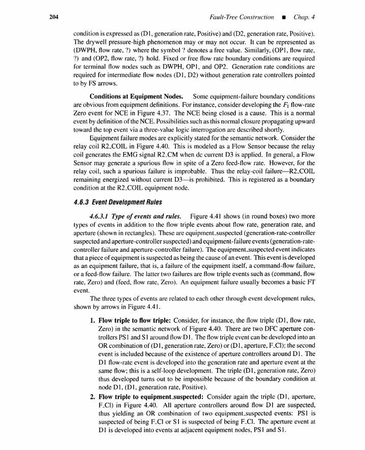
204 Fault-Tree Construction • Chap. 4
condition is expressed as (DI, generation rate, Positive) and (D2, generation rate, Positive).The drywell pressure-high phenomenon mayor may not occur. It can be represented as(DWPH, flow rate, 7) where the symbol 7 denotes a free value. Similarly, (OPI, flow rate,7) and (OP2, flow rate, 7) hold. Fixed or free flow rate boundary conditions are requiredfor terminal flow nodes such as DWPH, OPI, and OP2. Generation rate conditions arerequired for intermediate flow nodes (DI, D2) without generation rate controllers pointedto by FS arrows.
Conditions at Equipment Nodes. Some equipment-failure boundary conditionsare obvious from equipment definitions. For instance, consider developing the F1 flow-rateZero event for NCE in Figure 4.37. The NCE being closed is a cause. This is a normalevent by definitionof the NCE. Possibilities such as this normal closure propagating upwardtoward the top event via a three-value logic interrogation are described shortly.
Equipment failure modes are explicitly stated for the semantic network. Consider therelay coil R2_COIL in Figure 4.40. This is modeled as a Flow Sensor because the relaycoil generates the EMG signal R2_CM when de current D3 is applied. In general, a FlowSensor may generate a spurious flow in spite of a Zero feed-flow rate. However, for therelay coil, such a spurious failure is improbable. Thus the relay-coil failure-R2_COILremaining energized without current D3-is prohibited. This is registered as a boundarycondition at the R2_COIL equipment node.
4.6.3 Event Development Rules
4.6.3.1 Type of events and rules. Figure 4.41 shows (in round boxes) two moretypes of events in addition to the flow triple events about flow rate, generation rate, andaperture (shown in rectangles). These are equipment.suspected (generation-rate-controllersuspectedand aperture-controllersuspected) and equipment-failureevents (generation-rate-controller failure and aperture-controller failure). The equipment.suspected event indicatesthat a piece of equipment is suspected as being the cause of an event. This event isdevelopedas an equipment failure, that is, a failure of the equipment itself, a command-flow failure,or a feed-flow failure. The latter two failures are flow triple events such as (command, flowrate, Zero) and (feed, flow rate, Zero). An equipment failure usually becomes a basic FTevent.
The three types of events are related to each other through event development rules,shown by arrows in Figure 4.41.
1. Flow triple to flow triple: Consider, for instance, the flow triple (D1, flow rate,Zero) in the semantic network of Figure 4.40. There are two DFC aperture con-trollers PSI and S I around flow D I. The flow triple event can be developed into anOR combination of (DI, generation rate, Zero) or (DI, aperture, F_CI); the secondevent is included because of the existence of aperture controllers around D1. TheD1 flow-rate event is developed into the generation rate and aperture event at thesame flow; this is a self-loop development. The triple (D), generation rate, Zero)thus developed turns out to be impossible because of the boundary condition atnode D1, (D1, generation rate, Positive).
2. Flow triple to equipment-suspected: Consider again the triple (DI, aperture,F_CI) in Figure 4.40. All aperture controllers around flow D] are suspected,thus yielding an OR combination of two equipment.suspected events: PS1 issuspected of being F_CI or S1 is suspected of being F_CI. The aperture event atD1 is developed into events at adjacent equipment nodes, PS1 and S1.
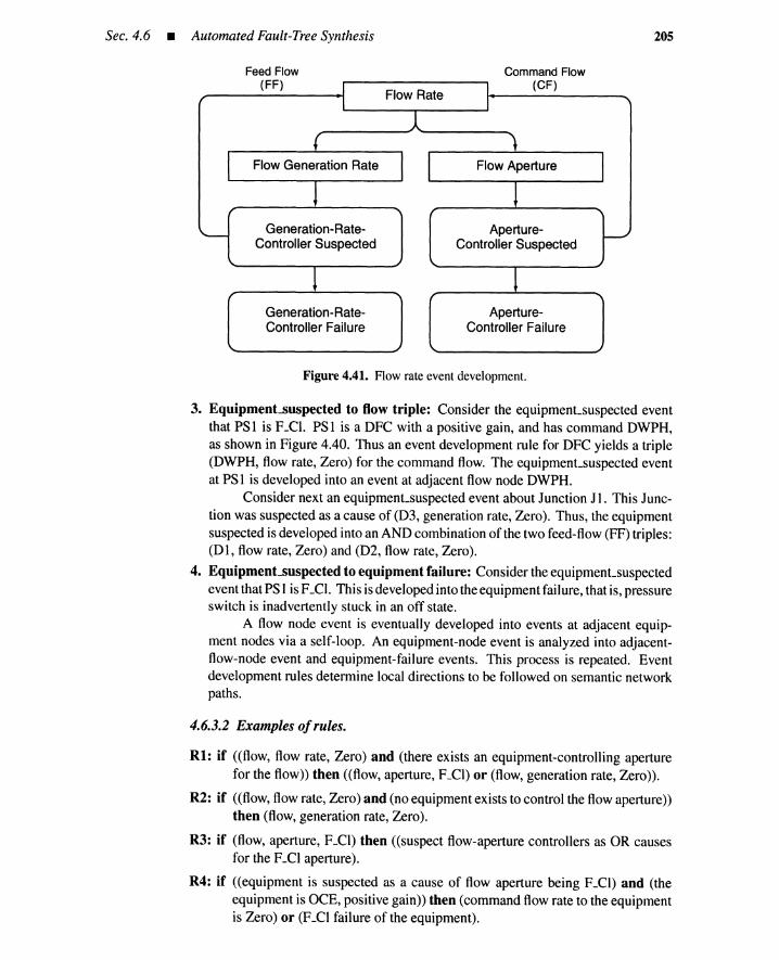
Sec.4.6 • Automated Fault-Tree Synthesis 205
Feed Flow(FF)
Command Flow(CF)
FlowGeneration Rate
Generation-Rate-ControllerSuspected
Generation-Rate-ControllerFailure
Flow Aperture
Aperture-ControllerSuspected
Aperture-ControllerFailure
Figure 4.41. Flow rate eventdevelopment.
3. Equipment-suspected to flow triple: Consider the equipment.suspected eventthat PS 1 is F.Cl. PS 1 is a DFC with a positive gain, and has command DWPH,as shown in Figure 4.40. Thus an event development rule for DFC yields a triple(DWPH, flow rate, Zero) for the command flow. The equipment.suspected eventat PS 1 is developed into an event at adjacent flow node DWPH.
Consider next an equipment.suspected event about Junction Jl. This Junc-tion was suspected as a cause of (D3, generation rate, Zero). Thus, the equipmentsuspected is developed into an AND combination of the two feed-flow (FF) triples:(D1, flow rate, Zero) and (D2, flow rate, Zero).
4. Equipment-suspected to equipment failure: Consider the equipment.suspectedevent that PS I is F_CI. This is developed into the equipment failure, that is, pressureswitch is inadvertently stuck in an off state.
A flow node event is eventually developed into events at adjacent equip-ment nodes via a self-loop. An equipment-node event is analyzed into adjacent-flow-node event and equipment-failure events. This process is repeated. Eventdevelopment rules determine local directions to be followed on semantic networkpaths.
4.6.3.2 Examples ofrules.
Rl: if ((flow, flow rate, Zero) and (there exists an equipment-controlling aperturefor the flow)) then ((flow, aperture, F_CI)or (flow, generation rate, Zero)).
R2: if ((flow, flow rate, Zero) and (no equipment exists to control the flow aperture))then (flow, generation rate, Zero).
R3: if (flow, aperture, F.Cl) then ((suspect flow-aperture controllers as OR causesfor the F.Cl aperture).
R4: if ((equipment is suspected as a cause of flow aperture being F_CI) and (theequipment is aCE, positive gain)) then (command flow rate to the equipmentis Zero) or (F_CI failure of the equipment).
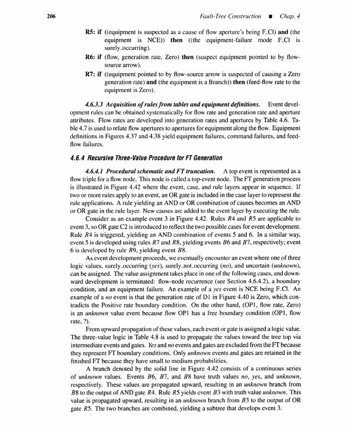
206 Fault-Tree Construction _ Chap. 4
R5: if «equipment is suspected as a cause of flow aperture's being F_Cl) and (theequipment is NCE» then «the equipment-failure mode F_Cl issurely.occurring).
R6: if (flow, generation rate, Zero) then (suspect equipment pointed to by flow-source arrow).
R7: if «equipment pointed to by flow-source arrow is suspected of causing a Zerogeneration rate) and (the equipment is a Branch» then (feed-flow rate to theequipment is Zero).
4.6.3.3 Acquisition ofrules from tables and equipment definitions. Event devel-opment rules can be obtained systematically for flow rate and generation rate and apertureattributes. Flow rates are developed into generation rates and apertures by Table 4.6. Ta-ble 4.7 is used to relate flow apertures to apertures for equipment along the flow. Equipmentdefinitions in Figures 4.37 and 4.38 yield equipment failures, command failures, and feed-flow failures.
4.6.4 Recursive Three-Value Procedure forFT Generation
4.6.4.1 Procedural schematic and FT truncation. A top event is represented as aflowtriple for a flow node. This node is called a top-event node. The FT generation processis illustrated in Figure 4.42 where the event, case, and rule layers appear in sequence. Iftwo or more rules apply to an event, an OR gate is included in the case layer to represent therule applications. A rule yielding an AND or OR combination of causes becomes an ANDor OR gate in the rule layer. New causes are added to the event layer by executing the rule.
Consider as an example event 3 in Figure 4.42. Rules R4 and R5 are applicable toevent 3, so OR gate C2 is introduced to reflect the two possible cases for event development.Rule R4 is triggered, yielding an AND combination of events 5 and 6. In a similar way,event 5 is developed using rules R7 and R8, yielding events B6 and B7, respectively; event6 is developed by rule R9, yielding event B8.
As event development proceeds, we eventuallyencounter an event where one of threelogic values, surely.occurring (yes), surely.not.occurring (no), and uncertain (unknown),can be assigned. The value assignment takes place in one of the followingcases, and down-ward development is terminated: flow-node recurrence (see Section 4.6.4.2), a boundarycondition, and an equipment failure. An example of a yes event is NCE being F_CI. Anexample of a no event is that the generation rate of D} in Figure 4.40 is Zero, which con-tradicts the Positive rate boundary condition. On the other hand, (OP}, flow rate, Zero)is an unknown value event because flow OPt has a free boundary condition (OP}, flowrate, ?).
From upwardpropagation of these values,each event or gate is assigned a logic value.The three-value logic in Table 4.8 is used to propagate the values toward the tree top viaintermediateevents and gates. Yesand no eventsand gates are excluded from the FT becausethey represent FT boundary conditions. Only unknown events and gates are retained in thefinished FT because they have small to medium probabilities.
A branch denoted by the solid line in Figure 4.42 consists of a continuous seriesof unknown values. Events B6, B7, and B8 have truth values no, yes, and unknown,respectively. These values are propagated upward, resulting in an unknown branch fromB8 to the output of AND gate R4. Rule R5 yields event B3 with truth value unknown. Thisvalue is propagated upward, resulting in an unknown branch from B3 to the output of ORgate R5. The two branches are combined, yielding a subtree that develops event 3.

Sec. 4.6 • AutomatedFault-Tree Synthesis 207
Rule
Rule
Rule
Case
Case
Event
Case
Event
Event
Event
u.........y::"\"\
[ C3 ':
n f··::::r::~...: y:"'."\ :,,1,,\
f R7 '~ f R8 ~·.··T· .....· .... ~ .....
n: :y, ........ , , .. _L_ ..,
( B6 :: ( B7 ::',- .....,' '........."
y: ....~ ..~
2 ~···fO··"y:
:,,1,,\
f R3 ':.... -;.....u r····~····: y# ..... ~, ,.-'-.,
:' B1 ': :' B2 ':, ,. ,'~._•• ,# '~•••• # •
Figure 4.42. Downward event development and upward truth propagation.
TABLE 4.8. Three-Value Logic for Upward Truth Value Propagation
A B AANDB AOR B
yesyesyesnononounknownunknownunknown
yesnounknownyesnounknownyesnounknown
yesnounknownnononounknownnounknown
yesyesyesyesnounknownyesunknownunknown
The general process illustrated in Figure 4.42 can be programmed into a recursiveprocedure that is a three-value generalization of a well-known backtracking algorithm [19].

208 Fault-Tree Construction _ Chap. 4
4.6.4.2 Flow-noderecurrence as house event. Consider the event, the flowrate ofR2_CMis Zero, in the network in Figure 4.40. A cause is a Zero-generation-rate event at thesame flow. This type of self-loop is required for a step-by-step eventdevelopment. However,because the flow node is in a loop, the same flow node, R2_CM, will be encountered forreasons other than the self-loop, that is, the recurrence occurs via other equipment or flownodes. To prevent infinite iterations of flow node, a truth value must be returned when aflow-node recurrence other than a self-loop type is encountered. The generation procedurereturns unknown. This means that a one-step-earlier event at the recurring flow node isincluded as a house event in the FT. As a result, one-step-earlier time series conditions arespecified for all recurrent flow nodes. The recurrence may occur for a flow node other thana top-event node.
As shown in Section 4.6.5.1, (R2_CM, flow rate, Zero) is included as a house eventfor the Zero R2_CM fault tree. If the house event is turned on, this indicates that the topevent continues to exist. On the other hand, turning off the house event means that theR2_CM flow rate changes from Positive to Zero. Different Ffs are obtained by assigningon-off values to house events.
4.6.4.3 FT module identification. Fault-tree modules considerably simplify Ffrepresentations, physical interpretations, and minimal cut set generations [20,2]].* Theproposed Ff generation approach enables us to identify Ff modules and their hierarchicalstructure.
Module flow node. Define the following symbols.
1. T: A top-event flow node.
2. N I: T: A flow node reachable from T. This ensures a possibility that the Ffgeneration procedure may encounter node N because the top-event developmenttraces the labeled arrows.
3. U(N): A set of flow nodes appearing in one or more paths from T to N. Node Nis excluded from the definition of U(N). Symbol U stands for upstream.
4. D(N): A set of flow nodes reachable from N where each reachability check pathis terminated immediately after it visits a node in U(N). Node N is removed fromthe definition of D(N). Symbol D stands for downstream.
5. R(N) == U(N) n D(N): A set of flow nodes commonly included in U(N) andD(N). This is a set of nodes in U(N) that may recur in D(N). Symbol R standsfor recurrence.
Consider, for instance, the semantic network in Figure 4.40. For top-event nodeT == R2_CM we observe:
U(01) == {R2_CM, D3},
U(D2) == {R2_CM, D3},
D(DI) == {aPI, DWPH},
D(D2) == {OP2, R2_CM},
R(D]) == 4> (4.1)
R(D2) == {R2_CM} (4.2)
Flow node N is called a module node when either condition C I or C2 holds. Modulenode N is displayed in Figure 4.43.
Cl: Sets U(N) and D(N) are mutually exclusive, that is, R(N) == 4>.C2: Each path from T to N has every node in R(N).
*Minimalcut sets are defined in Chapter 5.

Sec.4.6 • Automated Fault-Tree Synthesis
U(N)
00~-----+-----........
000000
:_-- -0 00-----' D(N)
Figure 4.43. Module flow node N.
209
Nodes D1 and D2 satisfy conditions C 1 and C2, respectively. Thus these are moduleflow nodes. The downstream development of a flow triple at node N remains identicalfor each access path through U(N) because neither node in U(N) recurs in D(N) whencondition Cl holds, and R(N) nodes recur in D(N) in the same way for each access pathfrom T to N when condition C2 holds. One or more identical subtrees may be generatedat node N, hence the name module flow node.
Repeated module node. Module node N is called a repeated module node whencondition C3 holds.
C3: Node N is reachable from T by two or more access paths. Neither node DI norD2 satisfies this condition.
Suppose that the FT generation procedure creates the same flow triple at node N bythe two or more access paths. This requirement is checked on-line, while conditions Clto C3 can be examined off-line by the semantic network before execution of FT genera-tion procedure. Two or more identical subtrees are generated for the same flow triple atnode N.
Another set of access paths may create a different flow triple. However, the uniqueflow triple is likely to occur because node N in a coherent system has a unique role incausing the top event. The repeated structure simplifies FT representation and Booleanmanipulations, although the structure cannot be replaced by a higher level basic eventbecause a subtree at node B of Figure 4.43 may appear both in node N subtree and node Asubtree. The repeated subtree is not a module in the sense of reference [20].
Solid-module node. Module node N is called a solid-module node when conditionC4 holds.
C4: Each node in D(N) is reachable from T only through N. In this case broken-line arrows do not exist in Figure 4.43. Nodes Dl and D2 are examples ofsolid-module nodes.
Suppose that the FT generation procedure creates a unique flow triple every time solid-module node N is visited through nodes in U(N). The uniqueness is likely to occur for a
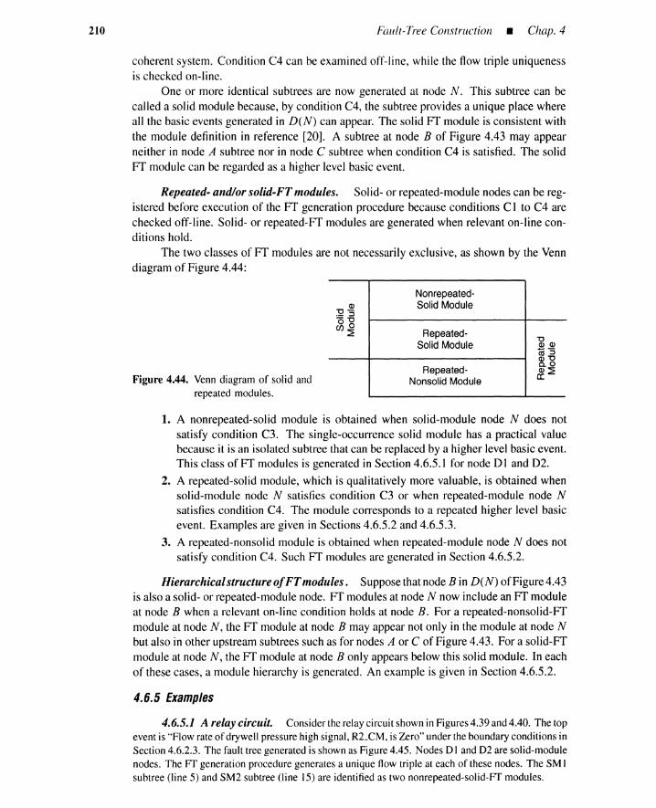
210 Fault-Tree Construction • Chap. 4
coherent system. Condition C4 can be examined off-line, while the flow triple uniquenessis checked on-line.
One or more identical subtrees are now generated at node N. This subtree can becalled a solid module because, by condition C4, the subtree provides a unique place whereall the basic events generated in D(N) can appear. The solid FT module is consistent withthe module definition in reference [20]. A subtree at node B of Figure 4.43 may appearneither in node A subtree nor in node C subtree when condition C4 is satisfied. The solidFT module can be regarded as a higher level basic event.
Repeated- and/or solid-FT modules. Solid- or repeated-module nodes can be reg-istered before execution of the FT generation procedure because conditions C I to C4 arechecked off-line. Solid- or repeated-FT modules are generated when relevant on-line con-ditions hold.
The two classes of FT modules are not necessarily exclusive, as shown by the Venndiagram of Figure 4.44:
Figure 4.44. Venn diagram of solid andrepeated modules.
Nonrepeated-0> Solid Module
"0-._ ::s0"8CJ)~ Repeated-
"0Solid Module 0> 0>co "3
0>"0
Repeated-0.0
Nonsolid Module£~
1. A nonrepeated-solid module is obtained when solid-module node N does notsatisfy condition C3. The single-occurrence solid module has a practical valuebecause it is an isolated subtree that can be replaced by a higher level basic event.This class of FT modules is generated in Section 4.6.5.1 for node D I and D2.
2. A repeated-solid module, which is qualitatively more valuable, is obtained whensolid-module node N satisfies condition C3 or when repeated-module node Nsatisfies condition C4. The module corresponds to a repeated higher level basicevent. Examples are given in Sections 4.6.5.2 and 4.6.5.3.
3. A repeated-nonsolid module is obtained when repeated-module node N does notsatisfy condition C4. Such FT modules are generated in Section 4.6.5.2.
Hierarchical structure ofFTmodules. Suppose that node B in D(N) of Figure4.43is also a solid- or repeated-module node. FT modules at node N now include an FT moduleat node B when a relevant on-line condition holds at node B. For a repeated-nonsolid-FTmodule at node N, the FT module at node B may appear not only in the module at node Nbut also in other upstream subtrees such as for nodes A or C of Figure 4.43. For a solid-FTmodule at node N, the FT module at node B only appears below this solid module. In eachof these cases, a module hierarchy is generated. An example is given in Section 4.6.5.2.
4.6.5 Examples
4.6.5.1 A relay circuit. Consider the relay circuit shown in Figures4.39 and 4.40. The topevent is "Flow rate of drywell pressure high signal, R2_CM, is Zero" under the boundary conditions inSection 4.6.2.3. The fault tree generated is shown as Figure 4.45. Nodes Oland 02 are solid-modulenodes. The Ff generation procedure generates a unique flow triple at each of these nodes. The SM1subtree (line 5) and SM2 subtree (line 15) are identified as two nonrepeated-solid-Ff modules.
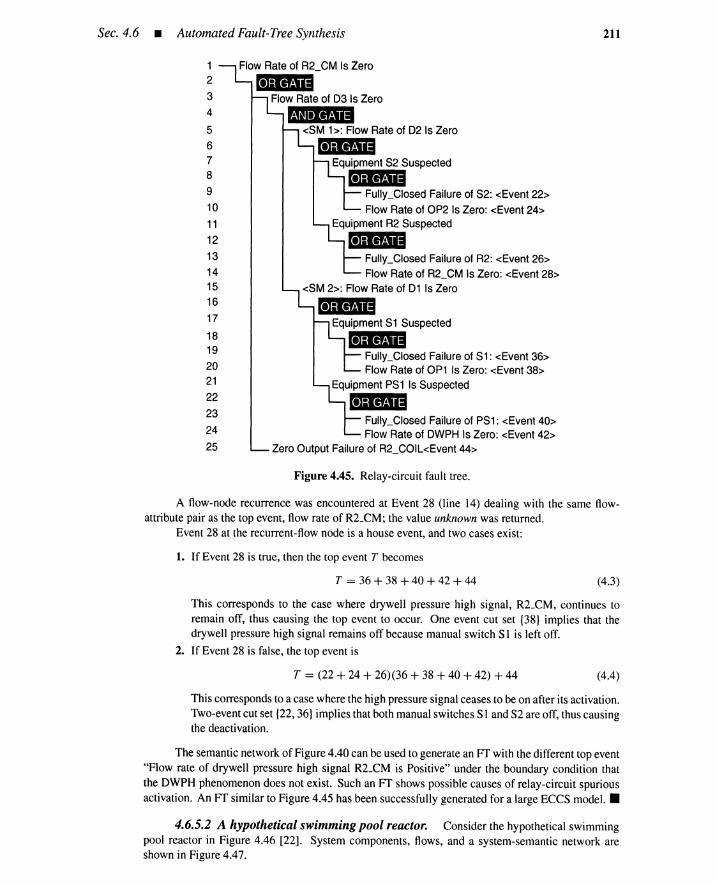
Sec. 4.6 • Automated Fault-Tree Synthesis 211
Flow Rateof R2_CM Is Zero
11&IIFlow Rateof 031s Zero-<SM 1>: Flow Rateof 02 Is Zero
11IIIEquipment S2 Suspected...
Fully_Closed Failureof S2: <Event22>Flow Rateof OP2 Is Zero: <Event24>
Equipment R2 Suspected...Fully_Closed Failureof R2: <Event26>Flow Rateof R2_CM Is Zero: <Event28>
<SM 2>: Flow Rateof 01 Is Zero-Equipment S1 Suspected...Fully_Closed Failureof S1: <Event36>Flow Rateof OP1 Is Zero: <Event38>
Equipment PS1 Is Suspected...Fully_Closed Failureof PS1:<Event40>Flow Rateof OWPH Is Zero: <Event42>
Zero Output Failureof R2_COIL<Event 44>
12
3
4
5
678
9
10
11
12
131415
16
17
1819
202122
23
24
25
Figure 4.45. Relay-circuit fault tree.
A flow-node recurrence was encountered at Event 28 (line 14) dealing with the same flow-attribute pair as the top event, flow rate of R2_CM; the value unknown was returned.
Event 28 at the recurrent-flow node is a house event, and two cases exist:
1. If Event 28 is true, then the top event T becomes
T = 36 + 38 + 40 + 42 + 44 (4.3)
This corresponds to the case where drywell pressure high signal, R2_CM, continues toremain off, thus causing the top event to occur. One event cut set {38} implies that thedrywell pressure high signal remains off because manual switch S1 is left off.
2. If Event 28 is false, the top event is
T = (22 + 24 + 26)(36 + 38 + 40 + 42) + 44 (4.4)
This corresponds to a case where the high pressure signal ceases to be on after its activation.Two-event cut set {22, 36} implies that both manual switches S 1and S2 are off, thus causingthe deactivation.
The semantic network of Figure 4.40 can be used to generate an FT with the different top event"Flow rate of drywell pressure high signal R2_CM is Positive" under the boundary condition thatthe DWPH phenomenon does not exist. Such an FT shows possible causes of relay-circuit spuriousactivation. An FT similar to Figure 4.45 has been successfully generated for a large ECCS model. •
4.6.5.2 A hypothetical swimming pool reactor. Consider the hypothetical swimmingpool reactor in Figure 4.46 [22]. System components, flows, and a system-semantic network areshown in Figure 4.47.
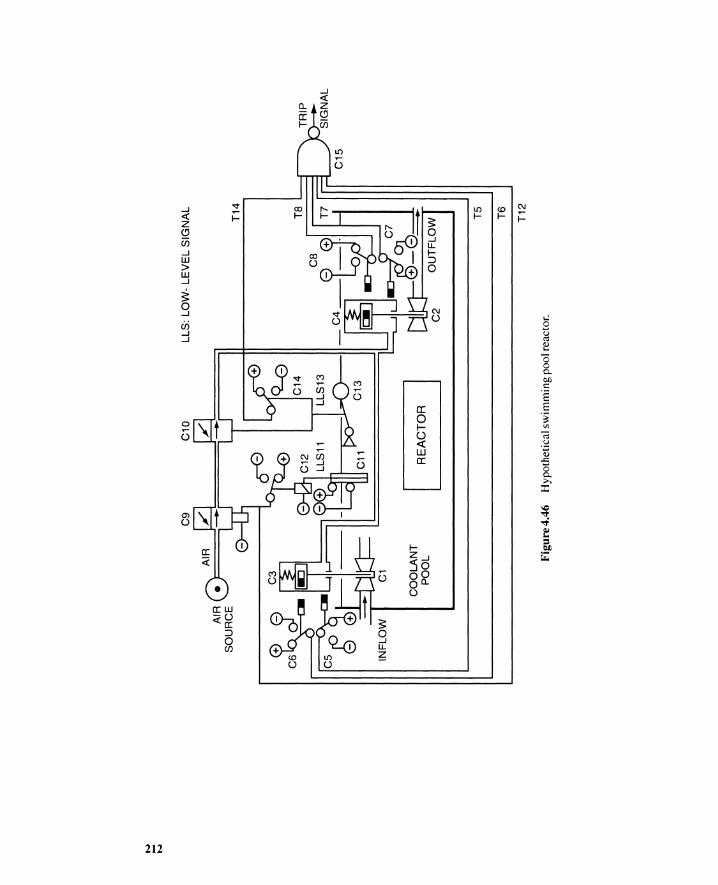
N ~ N
INF
LO
WI
C1
CO
OL
AN
TP
OO
L
C9
C10
IR
EA
CT
OR
I
LLS
:LO
W-
LE
VE
LS
IGN
AL
T14 T8
T5
T6
T12
C15
Fig
ure
4.46
Hyp
othe
tica
lsw
imm
ing
pool
reac
tor.
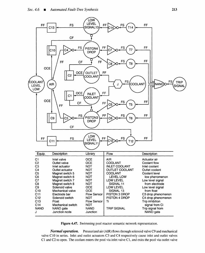
Sec. 4.6 • Automated Fault-Tree Synthesis 213
Equip. Description Library Flow Description
C1 Inlet valve aCE AIR Actuator airC2 Outlet valve aCE COOLANT Coolant flowC3 Inlet actuator NOT INLET COOLANT Inlet coolantC4 Outlet actuator NOT OUTLET COOLANT Outlet coolantC5 Magnet switch 5 NOT COOLANT Coolant levelC6 Magnet switch 6 NOT LEVEL LOW low phenomenonC7 Magnet switch 7 NOT LOW LEVEL Low level signalC8 Magnet switch 8 NOT SIGNAL 11 from electrodeC9 Solenoid valve aCE LOW LEVEL Low level signalC10 Mechanical valve aCE SIGNAL 13 from floatC11 Electrode bar Flow Sensor PISTON 3 DROP C3 drop phenomenonC12 Solenoid switch NOT PISTON 4 DROP C4 drop phenomenonC13 Float Flow Sensor Ti Trip inhibitionC14 Mechanical switch NOT signal from CiNAND NAND gate NAND TRIP SIGNAL Trip signal fromJ Junction node Junction NAND gate
Figure 4.47. Swimming pool reactor semantic network representation.
Normal operation. Pressurizedair (AIR) flows throughsolenoidvalveC9 and mechanicalvalve CIO in series. Inlet and outlet actuators C3 and C4 respectively cause inlet and outlet valvesCI and C2 to open. The coolant enters the pool via inlet valveCI, and exits the pool via outlet valve
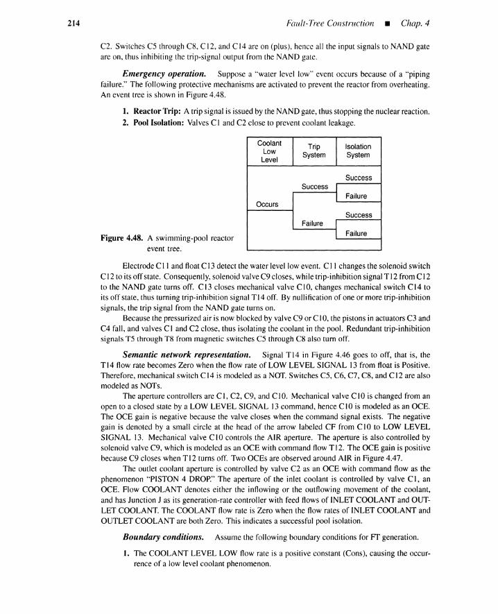
214 Fault-Tree Construction • Chap. 4
C2. Switches C5 through C8, C12,and C 14are on (plus), hence all the input signals to NAND gateare on, thus inhibiting the trip-signal output from the NAND gate.
Emergency operation. Suppose a "water level low" event occurs because of a "pipingfailure." The following protective mechanismsare activated to prevent the reactor from overheating.An event tree is shown in Figure 4.48.
1. Reactor Trip: A trip signal is issued by the NANDgate, thus stopping the nuclear reaction.2. Pool Isolation: Valves C I and C2 close to preventcoolant leakage.
Coolant Trip IsolationLow System SystemLevel
SuccessSuccess
FailureOccurs
SuccessFailure
FailureFigure 4.48. A swimming-pool reactorevent tree.
ElectrodeC I I and floatC13detect the water level lowevent. C II changes the solenoid switchC12to its off state. Consequently, solenoidvalveC9 closes, while trip-inhibitionsignalT 12from C12to the NAND gate turns off. C13 closes mechanical valve C I0, changes mechanical switch C14 toits off state, thus turning trip-inhibitionsignal TI4 off. By nullification of one or more trip-inhibitionsignals, the trip signal from the NAND gate turns on.
Because the pressurizedair is now blocked by valveC9 or CI0, the pistons in actuatorsC3 andC4 fall, and valvesC I and C2 close, thus isolating the coolant in the pool. Redundant trip-inhibitionsignals T5 through T8 from magnetic switches C5 through C8 also tum off.
Semantic network representation. Signal TI4 in Figure 4.46 goes to off, that is, theTI4 flow rate becomes Zero when the flow rate of LOW LEVEL SIGNAL 13 from float is Positive.Therefore, mechanical switch CI4 is modeled as a NOT. Switches C5, C6, C7, C8, and CI2 are alsomodeled as NOTs.
The aperture controllers are CI, C2, C9, and CIO. Mechanical valve CIO is changed from anopen to a closed state by a LOW LEVEL SIGNAL 13command, hence C lOis modeled as an OCE.The OCE gain is negative because the valve closes when the command signal exists. The negativegain is denoted by a small circle at the head of the arrow labeled CF from C I0 to LOW LEVELSIGNAL 13. Mechanical valve C10 controls the AIR aperture. The aperture is also controlled bysolenoid valveC9, which is modeled as an OCE with command flowT 12. The OCE gain is positivebecause C9 closes when T 12 turns off. Two OCEs are observed around AIR in Figure 4.47.
The outlet coolant aperture is controlled by valve C2 as an OCE with command flow as thephenomenon "PISTON 4 DROP." The aperture of the inlet coolant is controlled by valve C I, anOCE. Flow COOLANT denotes either the inflowing or the outflowing movement of the coolant,and has Junction J as its generation-rate controller with feed flows of INLET COOLANT and OUT-LET COOLANT. The COOLANT flow rate is Zero when the flow rates of INLET COOLANT andOUTLET COOLANT are both Zero. This indicates a successful pool isolation.
Boundary conditions. Assume the following boundary conditions for Fl' generation.
1. The COOLANT LEVEL LOW flow rate is a positive constant (Cons), causing the occur-rence of a low level coolant phenomenon.
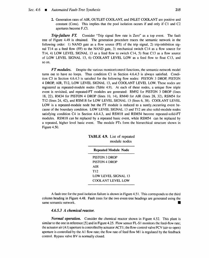
Sec. 4.6 • AutomatedFault-Tree Synthesis 215
2. Generation rates of AIR, OUTLET COOLANT, and INLET COOLANT are positive andconstant (Cons). This implies that the pool isolation occurs if and only if C 1 and C2apertures become F.Cl,
Trip-failure FT. Consider "Trip signal flow rate is Zero" as a top event. The faulttree of Figure 4.49 is obtained. The generation procedure traces the semantic network in thefollowing order: 1) NAND gate as a flow source (FS) of the trip signal, 2) trip-inhibition sig-nal T14 as a feed flow (FF) to the NAND gate, 3) mechanical switch C14 as a flow source forT14, 4) LOW LEVEL SIGNAL 13 as a feed flow to switch C14, 5) float C13 as a flow sourceof LOW LEVEL SIGNAL 13, 6) COOLANT LEVEL LOW as a feed flow to float C13, andso on.
FT modules. Despite the various monitor/control functions, the semantic-network modelturns out to have no loops. Thus condition C 1 in Section 4.6.4.3 is always satisfied. Condi-tion C3 in Section 4.6.4.3 is satisfied for the following flow nodes: PISTON 3 DROP, PISTON4 DROP, AIR, T12, LOW LEVEL SIGNAL 13, and COOLANT LEVEL LOW. These nodes areregistered as repeated-module nodes (Table 4.9). At each of these nodes, a unique flow tripleevent is revisited, and repeated-Ff modules are generated: RM92 for PISTON 3 DROP (lines18, 22), RM34 for PISTON 4 DROP (lines 10, 14), RM40 for AIR (lines 28, 32), RSM54 forT12 (lines 24, 42), and RSM18 for LOW LEVEL SIGNAL 13 (lines 6,38). COOLANT LEVELLOW is a repeated-module node but the FT module is reduced to a surely.occurring event be-cause of the boundary condition. LOW LEVEL SIGNAL 13 and T12 are also solid-module nodessatisfying condition C4 in Section 4.6.4.3, and RSM 18 and RSM54 become repeated-solid-FTmodules. RSM 18 can be replaced by a repeated basic event, while RSM54 can be replaced bya repeated, higher level basic event. The module FTs form the hierarchical structure shown inFigure 4.50.
TABLE 4.9. List of repeatedmodule nodes
Repeated Module Node
PISTON 3 DROPPISTON 4 DROP
AIR
T12LOW LEVEL SIGNAL 13
COOLANT LEVEL LOW
A fault tree for the pool isolation failure is shown in Figure 4.51. This corresponds to the thirdcolumn heading in Figure 4.48. Fault trees for the two event-tree headings are generated using thesame semantic network. •
4.6.5.3 A chemical reactor.
Normal operation. Consider the chemical reactor shown in Figure 4.52. This plant issimilar to the one in reference [5] and in Figure 4.25. Flow sensor FL-S 1 monitors the feed-flow rate;the actuator air (AI) aperture is controlled by actuator ACTl; the flow-control valve FCV (air-to-open)aperture is controlled by the A1 flow rate; the flow rate of feed flow M 1 is regulated by the feedbackcontrol. Bypass valve BV is normally closed.
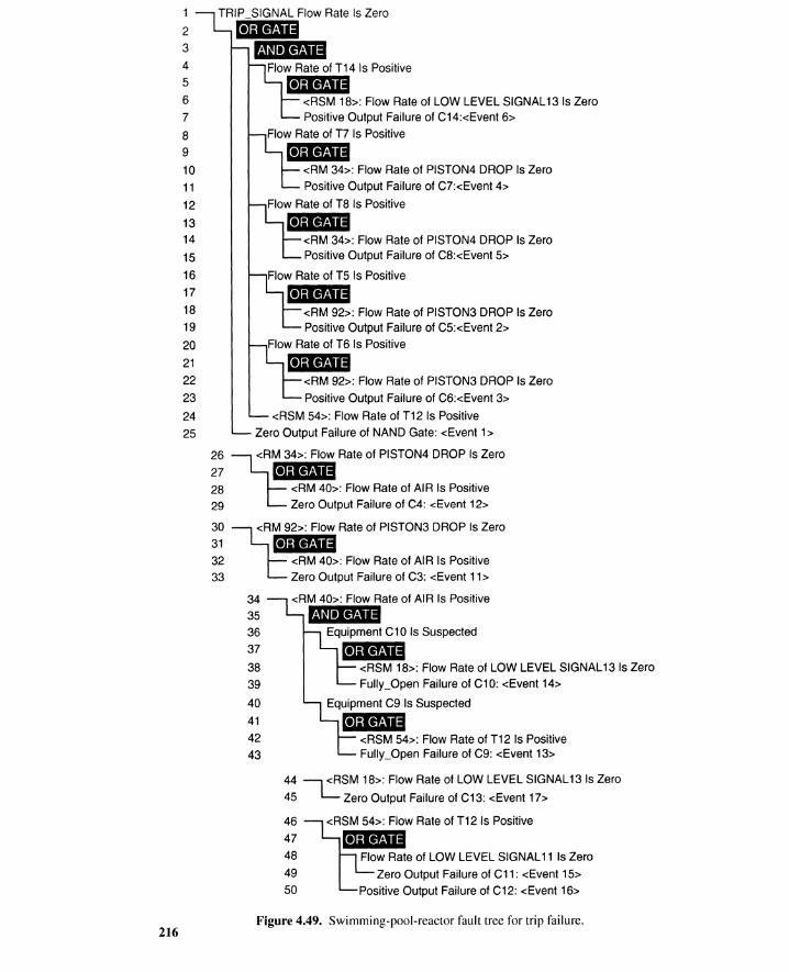
216
1 TRIP SIGNAL Flow Rate Is Zero2 _
3 ImIIim4 Flow Rate of T14 Is Positive
5 &JiI1ii6 <RSM 18>: Flow Rate of LOW LEVEL SIGNAL 13 Is Zero7 Positive Output Failure of C14:<Event 6>
8 Flow Rate of T7 Is Positive
9 &l1li10 <RM 34>: Flow Rate of PISTON4 DROP Is Zero
11 Positive Output Failure of C7:<Event 4>
12 Flow Rate of T8 Is Positive13 _
14 <RM 34>: Flow Rate of PISTON4 DROP Is Zero15 Positive Output Failure of C8:<Event 5>
16 Flow Rate of T5 Is Positive17 _
18 <RM 92>: Flow Rate of PISTON3 DROP Is Zero19 Positive Output Failure of C5:<Event 2>
20 Flow Rate of T6 Is Positive
21 &JiI1ii22 <RM 92>: Flow Rate of PISTON3 DROP Is Zero
23 Positive Output Failure of C6:<Event 3>
24 <RSM 54>: Flow Rate of T12 Is Positive
25 Zero Output Failure of NAND Gate: <Event 1>
26 ~RM34>: Flow Rate of PISTON4 DROP Is Zero27 _
28 <RM 40>: Flow Rate of AIR Is Positive29 Zero Output Failure of C4: <Event 12>
30 ~RM92>: Flow Rate of PISTON3 DROP Is Zero31 _
32 <RM 40>: Flow Rate of AIR Is Positive33 Zero Output Failure of C3: <Event 11>
34 <RM 40>: Flow Rate of AIR Is Positive35 _
36 Equipment C10 Is Suspected37 _
38 <RSM 18>: Flow Rate of LOW LEVEL SIGNAL 13 Is Zero39 Fully_Open Failure of C10: <Event 14>
40 Equipment C9 Is Suspected
41 BIll42 <RSM 54>: Flow Rate of T12 Is Positive43 Fully_Open Failure of C9: <Event 13>
44~SM 18>: Flow Rateof LOW LEVELSIGNAL13Is Zero
45 Zero Output Failure of C13: <Event 17>
46 <RSM 54>: Flow Rate of T12 Is Positive
47 &JiI1ii48 Flow Rate of LOW LEVEL SIGNAL 11 Is Zero
49 Zero Output Failure of C11: <Event 15>
50 Positive Output Failure of C12: <Event 16>
Figure 4.49. Swimming-pool-reactorfault tree for trip failure.
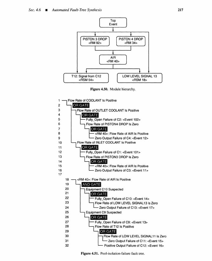
Sec.4.6 • Automated Fault-Tree Synthesis 217
T12: Signal from C12<RSM 54>
LOW LEVEL SIGNAL 13<RSM 18>
Figure 4.50. Modulehierarchy.
1
2
34
5
6
78
910
11
12
13
14
15
1617
18 <RM 40>: Flow Rate of AIR Is Positive19 _
20 Equipment C10 Suspected21 _
22 Fully_Open Failure of C10: <Event 14>
23 Flow Rate of LOW LEVEL SIGNAL 13 Is Zero
24 Zero Output Failure of C13: <Event 17>
25 Equipment C9 Suspected26 _
27 Fully_Open Failure of C9: <Event 13>28 Flow Rate of T12 Is Positive
29 &II1II30 Flow Rate of LOW LEVEL SIGNAL11 Is Zero
31 Zero Output Failure of C11: <Event 15>
32 Positive Output Failure of C12: <Event 16>
Figure 4.51. Pool-isolation-failure fault tree.

218
HORN PS2
Fault-Tree Construction • Chap. 4
ALARM
OP
FL-S1
BV
M4
•C3
.,...a:oI-U-cwa:
P1
TM-S1
C2
PUMP
Figure 4.52. Chemical reactor with control valve for feed shutdown.
Product PI from the reactor is circulated through heat exchanger HEXI by pump (PUMP).The product flow leaving the system through valve V is P3, which equals PI minus P2; flow PO is theproduct newly generated.
Automated emergency operation. Suppose that the feed M4 flow rate increases. Thechemical reaction is exothermic (releases heat) so a flowincreasecan create a dangerous temperatureexcursion. The temperature of product PI is monitored by temperature sensor TM-S1. A hightemperature activates actuator 2 (ACT2) to open the air A2 aperture, which in turn changes thenormally on pressure switch PSI (air-to-close) to its off state. The de current is cut off, and thenormally open solenoid valve (SLV; current-to-open) closes. Air AI is cut off, flow-control valveFCV is closed, feed M2 is cut off, and the temperature excursion is prevented. The FCV is used toshut down the feed, which, incidentally, is a dangerous design. It is assumed for simplicity that theresponse of the system to a feed shutdown is too slow to prevent a temperature excursion by loss ofheat exchanger cooling capability.
Manual emergency operation. A high-temperature measurement results in an air A4flow rate increase, which changes the normally off pressure switch PS2 (air-to-open) to an on state.The ac current activatesthe horn. The operator (OP) presses the normallyon panic button(BUTTON;operation-to-close) to change its state to off. The de current cut-off results in a feed shutdown.
New equipment and rules. A semantic network for the chemical reactor is shown inFigure 4.53. We see that heat exchanger HEXI cools product PI (CS: cold source), the coolant flowto the heat exchange is W (CLD_F: cold flow), product PO is generated by REACTORI (FS: flowsource), M4 is fed to the reactor (FF: feed flow), air A2 aperture is controlled by actuator ACT2, acommand flow of this actuator is command C3, this command is generated from temperature sensorTM-S I, and the temperature-sensorfeed flowis product PI.
Temperature sensor TM-SI, heat exchanger HEXI, and reactor REACTORI are three piecesof equipment not found in the equipment libraries. New event development rules specific to thesedevices are defined here. The proposed Fl-generation approach can be used for a variety of systemswith only the addition of new types of equipment and rules.
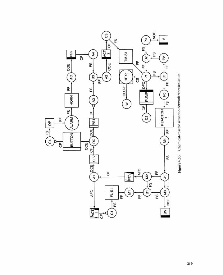
N ~ \C
AFC
FL
-S1
FS
Fig
ure
4.53
.C
hem
ical
-rea
ctor
sem
anti
c-ne
twor
kre
pres
enta
tion
.
TM
-S1
FS

220 Fault-Tree Construction • Chap. 4
Boundary conditions.
1. Flow rates of coolant Wand command C2 are subject to free boundary conditions.
2. Generation rates of M I, AI, A2, DC, and AC are positive constants (Cons).
Temperature-excursionFT with modules. Consider the topevent, temperatureincreaseof product P2. The semantic network of Figure 4.53 has three loops: one is loop P2-B2-PI-J2-P2;the other two start at PI and return to the same flow node via J2, J I, AI, DC, and B3.
The semantic network yields the following sets for node A2:
U(A2) = {P2,PI, PO, M4, M2, AI, DC, C4, ALARM, AC, A4, A3}D(A2) = {C3,PI}R(A2) = {PI}
Node A2 is a repeated-modulenode because conditions C2 and C3 are satisfied. We have long pathsfrom top-eventnode P2 to node A2. Fortunately,node AI turns out to be a nonrepeated-solid-modulenode satisfyingconditionsC2 and C4. These two module nodesare registered. The fault tree is shownin Figure 4.54. A nonrepeated-solid module SM65 for A1 is generated on line 16. Repeated-solidmodule RSM119appears twice in the SM65 tree (lines 41, 48).
The unknown house-event values generated at the flow-node recurrence are changed to no's,thus excluding one-step-earlier states. The top event occurs in the following three cases. The secondand the third correspond to cooling system failures.
1. Product PI temperature increase by feed-flow rate increase (line 3 of Figure 4.54)
2. Product P2 temperature increase by heat-exchangerfailure (line 17)
3. Product PI temperature increase by its aperture decrease (line 21)
The first case is divided into two causes: one is a feed M3 flow-rate increase because of abypass-valve failure (line 5), while the other is a feed M2 flow-rate increase (line 7) described byan AND gate (line 11), which has as its input a failure of protective action "closing valve Fey byshutting off air AI" (line 16). The protective-action failure is developed in the nonrepeated-solid-module tree labeled SM65 (line 25). Flow-rate values for free boundary-condition variables WandC2 are determined at event 200 (line 19) and 214 (line 24).
When cooling-system causes (200, 202, 212, and 214) are excluded, the top-eventexpressionbecomes
T = 49 + 165+ (182 + 192)[80 + 126+ 136+ (90 + III + 138+ 140) . 142)] (4.5)
One-event cut set {165} (line 9) implies a feed-flow-rate increase due to the FCY aperture increasefailure, a reflectionof the dangerous design. The largest cut set size is three; there are eight such cutsets. •
4.6.6 Summary
An automated fault-tree-generation method is presented. It is based on the flow,attribute, and value; an equipment library; a semantic-network representation of the system;event development rules; and a recursive three-value procedure with an Ff truncation andmodular-decomposition capability. Boundary conditions for the network can be specifiedat flow and equipment nodes. Event development rules are obtained systematically fromtables and equipment definitions. The three-value logic is used to truncate FTs accordingto boundary conditions. Only unknownevents or gates remain in the FT. Repeated- and/orsolid-FT modules and their hierarchies can be identified. From the same semantic-network-system model, different Fl's are generated for different top events and boundary conditions.
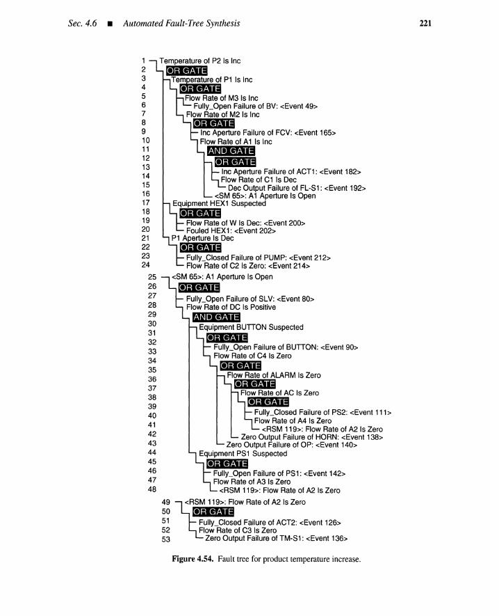
Sec. 4.6 • AutomatedFault-Tree Synthesis 221
Flow Rate of M3 Is IncFUlly_Open Failure of BV: <Event 49>
Flow Rate of M2 Is Inc[eli_j·,
Inc Aperture Failure of FCV: <Event 165>Flow Rate of A1 Is Inc
m" ••j':I[eli'.41·,
Inc Aperture Failure of ACT1: <Event 182>Flow Rate of C1 Is Dec
Dec Output Failure of FL-S1: <Event 192><SM 65>: A1 Aperture Is Open
Equipment HEX1 Suspected[eli_j·,
Flow Rate of W Is Dec: <Event 200>Fouled HEX1: <Event 202>
P1 Aperture Is Dec[elil"i.,
Fully_Closed Failure of PUMP: <Event 212>Flow Rate of C2 Is Zero: <Event 214>
<SM 65>: A1 Aperture Is Open
[eliB"Fully_Open Failure of SLV: <Event 80>Flow Rate of DC Is Positive
ml '••"!Equipment BUTTON Suspected
[eJi_"pFully_Open Failure of BUTTON: <Event 90>Flow Rate of C4 Is Zero
[eli_4.,Flow Rate of ALARM Is Zero
[elien·!Flow Rate of AC Is Zero[eli_4.,
Fully_Closed Failure of PS2: <Event 111>Flow Rate of A4 Is Zero
<RSM 119>: Flow Rate of A2 Is ZeroZero Output Failure of HORN: <Event 138>
Zero Output Failure of OP: <Event 140>Equipment PS1 Suspected
[el;Mj"Fully_Open Failure of PS1: <Event 142>Flow Rate of A31s Zero
<RSM 119>: Flow Rate of A2 Is Zero
49 ~RSM 119>: Flow Rate of A2 Is Zero50 [eli_41"51 Fully_Closed Failure of ACT2: <Event 126>52 Flow Rate of C3 Is Zero53 Zero Output Failure of TM-S1: <Event 136>
Temperature of P2 Is Inc[el.i••
Tern erature of P1 Is Inc.-123456789101112131415161718192021222324
252627282930313233343536373839404142434445464748
Figure 4.54. Fault tree for producttemperature increase.
222 Fault-Tree Construction _ Chap. 4
The generation method is demonstrated for a relay system, a hypothetical swimming-pool reactor, and a chemical reactor.
REFERENCES
[I] Fussell, J. B. "Fault tree analysis: Concepts and techniques." In Proc. of the NATOAdvanced Study Institute on Generic Techniques in Systems Reliability Assessment,edited by E. Henley and J. Lynn, pp. 133-162. Leyden, Holland: NoordhoffPublishingCo., 1976.
[2] Fussell, J. B., E. F. Aber, and R. G. Rahl. "On the quantitative analysis of priorityAND failure logic," IEEE Trans. on Reliability, vol. 25, no. 5, pp. 324-326, 1976.
[3] Lambert, H. E. "System safety analysis and fault tree analysis." Lawrence LivermoreLaboratory, UCID-16238, May 1973.
[4] Barlow, R. E., and F. Proschan. Statistical Theory of Reliability and Life TestingProbability Models. New York: Holt, Rinehart and Winston, 1975.
[5] Browning, R. L. "Human factors in fault trees," Chem. Engingeering Progress, vol. 72,no.6,pp. 72-75,1976.
[6] Henley, E. J., and H. Kumamoto. Reliability Engineering and Risk Assessment.Englewood Cliffs, NJ: Prentice-Hall, 1981.
[7] Henley, E. J., and H. Kumamoto. Probabilistic Risk Assessment. New York: IEEEPress, 1992.
[8] Vesely, W. E. "Reliability and fault tress applications at the NRTS," IEEE Trans. onNucl. Sci., vol. I, no. I, pp. 472-480,1971.
[9] Barlow, R. E., and E. Proschan. Statistical Theory of Reliability and Life TestingProbability Models. New York: Holt, Rinehart and Winston, 1975.
[10] Andrews, J., and G. Brennan. "Application of the digraph method of fault tree con-struction to a complex control configuration," Reliability Engineering and SystemSafety, vol. 28, no. 3, pp. 357-384, 1990.
[II] Chang, C. T., and K. S. Hwang. "Studies on the digraph-based approach for fault-treesynthesis. I. The ratio-control systems," Industrial Engineering Chemistry Research,vol. 33,no.6,pp. 1520-1529, 1994.
[12] Chang, C. T., D. S. Hsu, and D. M. Hwang. "Studies on the digraph-based approach forfault-tree synthesis. 2. The trip systems," Industrial Engineering Chemistry Research,vol. 33, no. 7,pp. 1700-1707, 1994.
[13] Kelly, B. E., and F. P. Lees. "The propagation of faults in process plants, Parts 1-4,"Reliability Engineering, vol. 16, pp. 3-38, pp. 39--62, pp. 63-86, pp. 87-108, 1986.
[14] Mullhi, J. S., M. L. Ang, F. P. Lees, and J. D. Andrews. "The propagation of faults inprocess plants, Part 5," Reliability Engineering and SystemSafety, vol. 23, pp. 31-49,1988.
[15] Hunt, A., B. E. Kelly, J. S. Mullhi, F. P. Lees, and A. G. Rushton. "The propagationof faults in process plants, Parts 6-10," Reliability Engineering and System Safety,vol. 39,pp. 173-194,pp. 195-209,pp.211-227,pp. 229-241,pp. 243-250, 1993.
[16] Fussell, J. B. "A formal methodology for fault tree construction," Nuclear ScienceEngineering, vol. 52, pp. 421-432, 1973.
[17] Salem, S. L., G. E. Apostolakis, and D. Okrent. "A new methodology for the computer-aided construction of fault trees," Annals ofNuclear Energy, vol. 4, pp. 417-433, 1977.
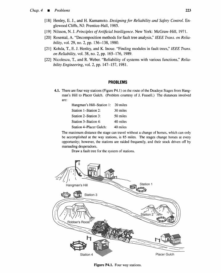
Chap. 4 • Problems 223
[18] Henley, E. J., and H. Kumamoto. Designing for Reliability and Safety Control . En-glewoodCliffs, NJ: Prentice-Hall, 1985.
[19] Nilsson, N. J. Principles ofArtificial Intelligence. New York: McGraw-Hill, 1971.
[20] Rosental, A. "Decomposition methods for fault tree analysis," IEEE Trans. on Relia-bility, vol. 29, no. 2, pp. 136-138, 1980.
[21] Kohda, T., E. J. Henley, and K. Inoue. "Finding modules in fault trees," IEEE Trans.on Reliability, vol. 38, no. 2, pp. 165-176, 1989.
[22] Nicolescu, T., and R. Weber. "Reliability of systems with various functions," Relia-bility Engineering, vol. 2, pp. 147-157, 1981.
PROBLEMS
4.1. There are four way stations (Figure P4.1) on the route of the Deadeye Stages from Hang-man's Hill to Placer Gulch. (Problem courtesy of J. Fussell.) The distances involvedare:
Hangman's Hill-Station I: 20 miles
Station I-Station 2: 30 miles
Station 2-Station 3: 50 miles
Station 3-Station 4: 40 miles
Station 4-Placer Gulch: 40 miles
The maximum distance the stage can travel without a change of horses, which can onlybe accomplished at the way stations, is 85 miles. The stages change horses at everyopportunity; however, the stations are raided frequently, and their stock driven off bymarauding desperadoes .
Draw a fault tree for the system of stations.
Hangman's Hill
Placer Gulch
Figure P4.1. Four way stations.
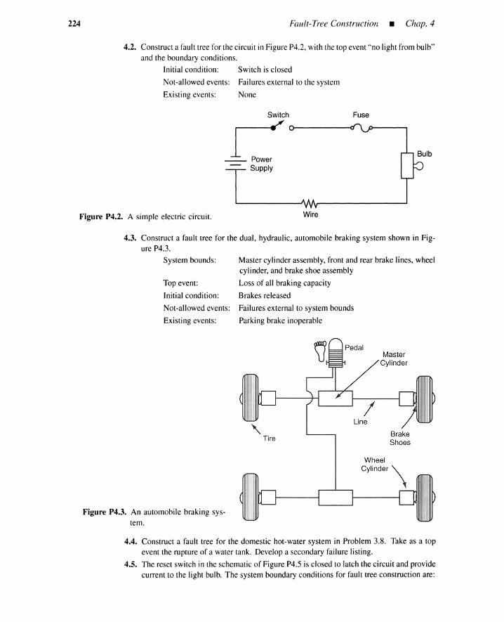
224 Fault-Tree Construction • Chap. 4
4.2. Constructa faulttree for thecircuit in FigureP4.2, with the topeventvno light from bulb"and the boundary conditions.
Initial condition: Switch is closed
Not-allowed events: Failuresexternal to the system
Existing events: None
Figure P4.2. A simple electric circuit.
Switch
CSupply
Wire
Fuse
4.3. Construct a fault tree for the dual, hydraulic, automobile braking system shown in Fig-ure P4.3.
System bounds: Master cylinderassembly, front and rear brake lines, wheelcylinder, and brakeshoe assembly
Topevent: Loss of all brakingcapacity
Initialcondition: Brakes released
Not-allowed events: Failuresexternal to system bounds
Existingevents: Parkingbrake inoperable
"- Ti re
Line
MasterCylinder
BrakeShoes
Figure P4.3. An automobile braking sys-tem.
4.4. Construct a fault tree for the domestic hot-watersystem in Problem 3.8. Take as a topevent the ruptureof a water tank. Develop a secondary failure listing.
4.5. The reset switch in the schematicof FigureP4.5 is closed to latch the circuit and providecurrent to the light bulb. The system boundaryconditionsfor fault tree construction arc:
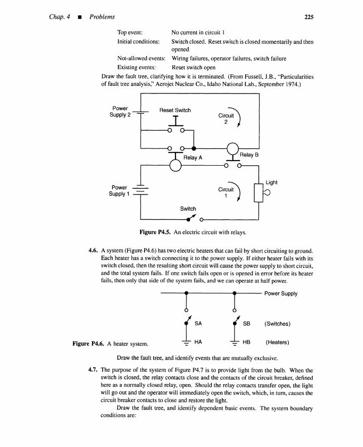
Chap. 4 • Problems 225
Top event:
Initial conditions:
No current in circuit 1
Switch closed. Reset switch is closed momentarily and thenopened
Not-allowed events: Wiring failures, operator failures, switch failure
Existing events: Reset switch open
Draw the fault tree, clarifying how it is terminated. (From Fussell, J.B., "Particularitiesof fault tree analysis," Aerojet Nuclear Co., Idaho National Lab., September 1974.)
PowerSupply 2
Reset Switch
.r, Cir~:;;;
Relay B
1 Switch____.' {}--__-.I
PowerSupply 1
Figure P4.5. An electric circuit with relays.
4.6. A system (Figure P4.6) has two electric heaters that can fail by short circuiting to ground.Each heater has a switch connecting it to the power supply. If either heater fails with itsswitch closed, then the resulting short circuit will cause the power supply to short circuit,and the total system fails. If one switch fails open or is opened in error before its heaterfails, then only that side of the system fails, and we can operate at half power.
(Heaters)
(Switches)
Figure P4.6. A heater system.
ri SA
- HA
r---- Power Supply
i S8
- HB
Draw the fault tree, and identify events that are mutually exclusive.
4.7. The purpose of the system of Figure P4.7 is to provide light from the bulb. When theswitch is closed, the relay contacts close and the contacts of the circuit breaker, definedhere as a normally closed relay, open. Should the relay contacts transfer open, the lightwill go out and the operator will immediately open the switch, which, in tum, causes thecircuit breaker contacts to close and restore the light.
Draw the fault tree, and identify dependent basic events. The system boundaryconditions are:
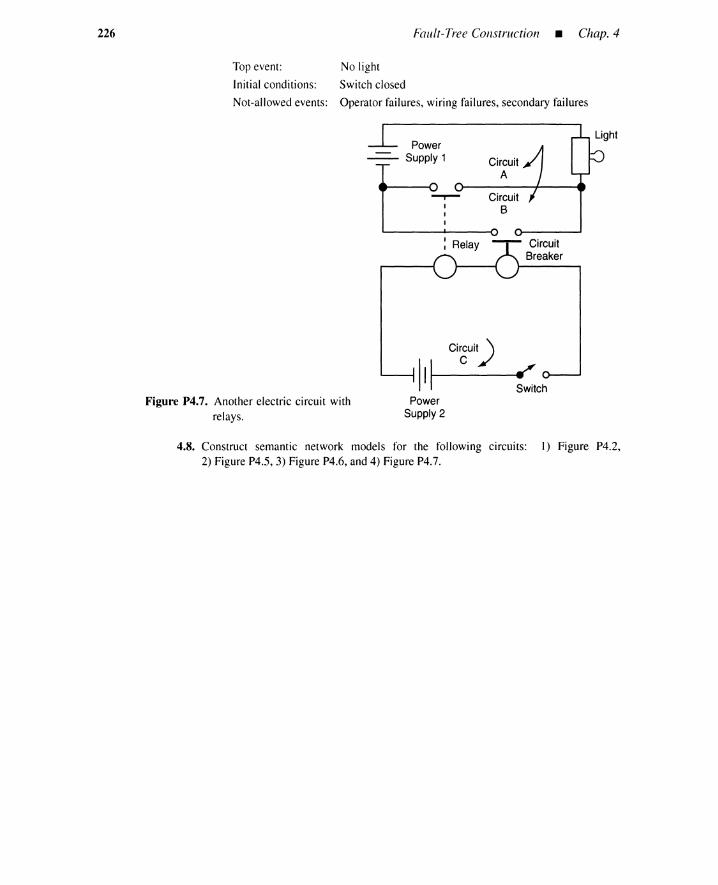
226
Top event:
Initial conditions:
Not-allowedevents:
Fault-Tree Construction • Chap. 4
No light
Switch closed
Operator failures, wiring failures, secondary failures
PowerSupply 1 Circuit
A
CircuitB
CircuitBreaker
Figure P4.7. Another electric circuit withrelays.
PowerSupply2
4.8. Construct semantic network models for the following circuits: 1) Figure P4.2,2) Figure P4.5, 3) Figure P4.6, and 4) Figure P4.7.
ualitative Aspectsof System Analysis
5.1 INTRODUCTION
System failures occur in many ways. Each unique way is a system-failure mode, involvingsingle- or multiple-component failures. To reduce the chance of a system failure, we mustfirst identify the failure modes and then eliminate the most frequently occurring and/orhighly probable. The fault-tree methods discussed in the previous chapter facilitate thediscovery of failure modes; the analytical methods described in this chapter are predicatedon the existence of fault trees.
5.2 CUT SETS AND PATH SETS
5.2.1 Cut Sets
For a given fault tree, a system-failure mode is clearly defined by a cut set, which isa collection of basic events; if all basic events occur, the top event is guaranteed to occur.Consider, for example, the fault tree of Figure 5.1, which is a simplified version of Figure4.24 after removal of secondary failures. If events 2 and 4 occur simultaneously, the topevent occurs, that is, if "contacts failure (stuck closed)" and "switch failure (stuck closed)"coexist, the top event, "pressure tank rupture," happens. Thus set {2,4} is a cut set. Also,{I} and {3,5} are cut sets.
Figure 5.2 is a reliability block-diagram representation equivalent to Figure 5.1. Weobserve that each cut set disconnects left and right terminal nodes denoted by circles.
5.2.2 Path Sets (Tie Sets)
A path set is the dual concept of a cut set. It is a collection of basic events, and ifnone of the events in the set occur, the non-occurrence of the top event is guaranteed. When
227

228 Qualitative Aspects ofSystem Analysis • Chap. 5
2 3 4
5 6
Figure 5.1. A pressure-tank-rupturefault tree.
I\ C J'------------
/--------------------~
I ----------- II II I
IIIII II \ E JI '- _
I \ 0 J II ,-------------------~l .-J
l,---------------------------------~
.: - ~- - -r---.:----------.:--.:---------------------------------- ~l: ----------- B:IIIIII
Figure 5.2. A pressure-tank-rupturereliability block diagram.
the system has only one top event, the non-occurrence of the basic failure events in a
path set ensures successful system operation. The non-occurrence does not guarantee
system success when more than one top event is specified. In such cases, a path set only

Sec. 5.2 • Cut Sets and Path Sets 229
ensures the non-occurrence of a particular top event. A path set is sometimes called atie set.
For the fault tree of Figure 5.1, if failure events 1, 2, and 3 do not occur, the top eventcannot happen. Hence if the tank, contacts, and timer are normal, the tank will not rupture.Thus {1,2,3} is a path set. Another path set is {I,4,5,6}, that is, the tank will not rupture ifthese failure events do not happen. In terms of the reliability block diagram of Figure 5.2,a path set connects the left and right terminal nodes.
5.2.3 Minimal Cut Sets
A large system has an enormous number of failure modes; hundreds of thousandsof cut sets are possible for systems having between 40 and 90 components. If there arehundreds of components, billions of cut sets may exist. To simplify the analysis, it isnecessary to reduce the number of failure modes. We require only those failure modes thatare general, in the sense that one or more of them must happen for a system failure to occur.Nothing is lost by this restriction. If it were possible to improve the system in such a wayas to eliminate all general failure modes, that would automatically result in the eliminationof all system-failure modes.
A minimal cut set clearly defines a general failure mode. A minimal cut set is suchthat, if any basic event is removed from the set, the remaining events collectively are nolonger a cut set. A cut set that includes some other sets is not a minimal cut set. Theminimal-cut-set concept enables us to reduce the number of cut sets and the number ofbasic events involved in each cut set. This simplifies the analysis.
The fault tree of Figure 5.1 has seven minimal cut sets {1}, {2,4}, {2,5}, {2,6}, {3,4},{3,5}, {3,6}. Cut set {1,2,4} is not minimal because it includes {I} or {2,4}. Both failuremodes {1} and {2,4} must occur for mode {1,2,4} to occur. All failure modes are preventedfrom occurring when the modes defined by the minimal cut sets are eliminated.
5.2.4 Minimal Path Sets
A minimal path set is a path set such that, if any basic event is removed from the set,the remaining events collectively are no longer a path set. The fault tree of Figure 5.1 hastwo minimal path sets, {1,2,3} and {1,4,5,6}. If either {1,2,3} or {1,4,5,6} do not fail, thetank operates.
5.2.5 Minimal Cut Generation (Top-Down)
The MOCUS (method of obtaining cut sets) computer code can be used to generateminimal cut sets [1]. It is based on the observation that OR gates increase the number ofcut sets, whereas AND gates enlarge the size of the cut sets. The MOCUS algorithm canbe stated as follows.
1. Alphabetize each gate.
2. Number each basic event.
3. Locate the uppermost gate in the first row of a matrix.
4. Iterate either of the fundamental permutations a or b below in a top-down fashion.(When intermediate events are encountered, replace them by equivalent gates orbasic events.)(a) Replace an OR gate by a vertical arrangement of the input to the gate, and
increase the number of cut sets.
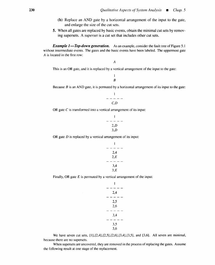
230 Qualitative Aspects of System Analysis _ Chap. 5
(b) Replace an AND gate by a horizontal arrangement of the input to the gate,and enlarge the size of the cut sets.
5. When all gates are replaced by basic events, obtain the minimal cut sets by remov-ing supersets. A superset is a cut set that includes other cut sets.
Example 1-Top-down generation. As an example, consider the fault tree of Figure 5.1without intermediate events. The gates and the basic events have been labeled. The uppermost gateA is located in the first row:
A
This is an OR gate, and it is replaced by a vertical arrangement of the input to the gate:
IB
Because B is an AND gate, it is permuted by a horizontal arrangement of its input to the gate:
C,D
OR gate C is transformed into a vertical arrangement of its input:
2,D3,D
OR gate D is replaced by a vertical arrangement of its input:
2,42,E
3,43,E
Finally,OR gate E is permuted by a vertical arrangement of the input:
2,4
2,5
2,6
3,4
3,53,6
We have seven cut sets, {I},{2,4},{2,5},{2,6},{3,4},{3,5}, and {3,6}. All seven are minimal,because there are no supersets.
When supersets are uncovered, theyare removedin the process of replacing the gates. Assumethe following result at one stage of the replacement.

Sec. 5.2 • Cut Sets and Path Sets
1,2,G1,2,3,G1,2,K
231
A cut set derived from {1,2,3,G} always includes a set from {I,2,G}. However, the cut set from{1,2,3,G} may not include any sets from {I,2,K} because the developmentof K may differ from thatof G. We have the following simplifiedresult:
1,2,G1,2,K
When an event appears more than two times in a horizontal arrangement, it is aggregated intoa single event. For example, the arrangement {1,2,3,2,H} should be changed to {1,2,3,H}. Thiscorresponds to the idempotence rule of Boolean algebra: 2 AND 2 =2.* •
Example 2-Boolean top-down generation. The fault tree of Figure 5.1 can be repre-sented by a set of Boolean expressions:
A= I +B,D =4+ E,
B=C·D,E = 5+6
C=2+3 (5.1)
The top-down algorithm corresponds to a top-down expansion of the top gate A.
A = 1 + B = I + C . D (5.2)
I + (2 + 3) . D = 1 + 2 . D + 3 . D (5.3)
= 1 + 2 . (4 + E) + 3 . (4 + E) = I + 2 ·4+ 2 . E + 3 ·4+ 3 . E (5.4)
= 1 + 2 ·4+ 2 . (5 + 6) + 3 ·4+ 3 . (5 + 6) (5.5)
= 1 + 2 . 4 + 2 . 5 + 2 . 6 + 3 . 4 + 3 . 5 + 3 . 6 (5.6)
where a centered dot (.) and a plus sign (+) stand for AND and OR operations, respectively. The dotsymbol is frequently omitted when there is no confusion.
The above expansion can be expressed in matrix form:
I2 43 5
6
I2·42·52·63·43·53·6
(5.7)
•5.2.6 Minimal Cut Generation (Bottom-Up)
MOCUS is based on a top-down algorithm. MICSUP (minimal cut sets, upward) [2] isa bottom-up algorithm. In the bottom-up algorithm, minimal cut sets of an upper-level gateare obtained by substituting minimal cut sets of lower-level gates. The algorithm starts withgates containing only basic events, and minimal cut sets for these gates are obtained first.
Example 3-Boolean bottom-up generation. Consider again the fault tree of Figure5.1. The minimal cut sets of the lowest gates, C and E, are:
C = 2+3
E = 5+6
*See appendix to Chapter 3 for Boolean operations and laws.
(5.8)
(5.9)
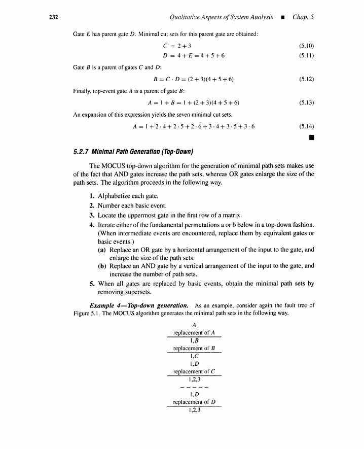
232 Qualitative Aspects ofSystem Analysis • Chap. 5
Gate E has parent gate D. Minimalcut sets for this parent gate are obtained:
C = 2+3
D = 4+£=4+5+6
Gate B is a parent of gates C and D:
B = C . D = (2 + 3)(4 + 5 + 6)
Finally, top-eventgate A is a parent of gate B:
A = 1 + B = 1 + (2 + 3)(4 + 5 + 6)
An expansion of this expressionyields the seven minimalcut sets.
A= 1+2·4+2·5+2·6+3·4+3·5+3·6
5.2.7 Minimal Path Generation (Top-Down)
(5.10)
(5.11)
(5.12)
(5.13)
(5.14)
•The MOCUS top-down algorithm for the generation of minimal path sets makes use
of the fact that AND gates increase the path sets, whereas OR gates enlarge the size of thepath sets. The algorithm proceeds in the following way.
1. Alphabetize each gate.
2. Number each basic event.
3. Locate the uppermost gate in the first row of a matrix.
4. Iterate either of the fundamental permutations a or b below in a top-down fashion.(When intermediate events are encountered, replace them by equivalent gates orbasic events.)(a) Replace an OR gate by a horizontal arrangement of the input to the gate, and
enlarge the size of the path sets.(b) Replace an AND gate by a vertical arrangement of the input to the gate, and
increase the number of path sets.
5. When all gates are replaced by basic events, obtain the minimal path sets byremoving supersets.
Example 4-Top-down generation. As an example, consider again the fault tree ofFigure 5.1. The MOCUS algorithm generates the minimal path sets in the following way.
Areplacementof A
I,Breplacementof B
I,CI,D
replacementof C1,2,3
I,Dreplacementof D
1,2,3
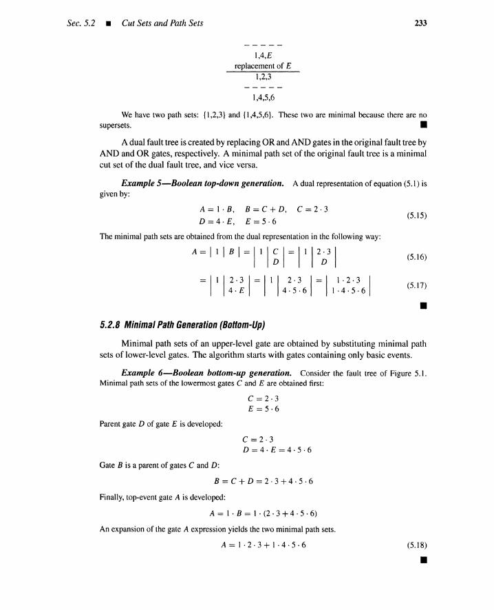
Sec. 5.2 • Cut Sets and Path Sets
1,4,Ereplacement of E
1,2,3
1,4,5,6
233
We have two path sets: {I,2,3} and {I,4,5,6}. These two are minimal because there are nosupersets. •
A dual fault tree is created by replacing OR and AND gates in the original fault tree byAND and OR gates, respectively. A minimal path set of the original fault tree is a minimalcut set of the dual fault tree, and vice versa.
Example 5-Boolean top-downgeneration. A dual representation of equation (5.1) isgiven by:
A = 1· B,
D=4·E,
B = C + D,
E = 5·6
C = 2· 3(5.15)
The minimal path sets are obtained from the dual representation in the following way:
A = I I B I = 11 I ~ I = 11 12~31 (5.16)
= 11 I;.' ~ 1= 11 I/; ~ 61 = 11 ~ / ; ~ 61 (5.17)
•5.2.8 Minimal Path Generation (Bottom-Up)
Minimal path sets of an upper-level gate are obtained by substituting minimal pathsets of lower-level gates. The algorithm starts with gates containing only basic events.
Example 6-Boolean bottom-up generation. Consider the fault tree of Figure 5.1.Minimal path sets of the lowermost gates C and E are obtained first:
C = 2·3E = 5·6
Parent gate D of gate E is developed:
C = 2·3D=4·E=4·5·6
Gate B is a parent of gates C and D:
B=C+D=2·3+4·5·6
Finally, top-event gate A is developed:
A = 1 . B = 1 . (2 . 3 + 4 . 5 . 6)
An expansion of the gate A expression yields the two minimal path sets.
A=1·2·3+1·4·5·6 (5.18)
•
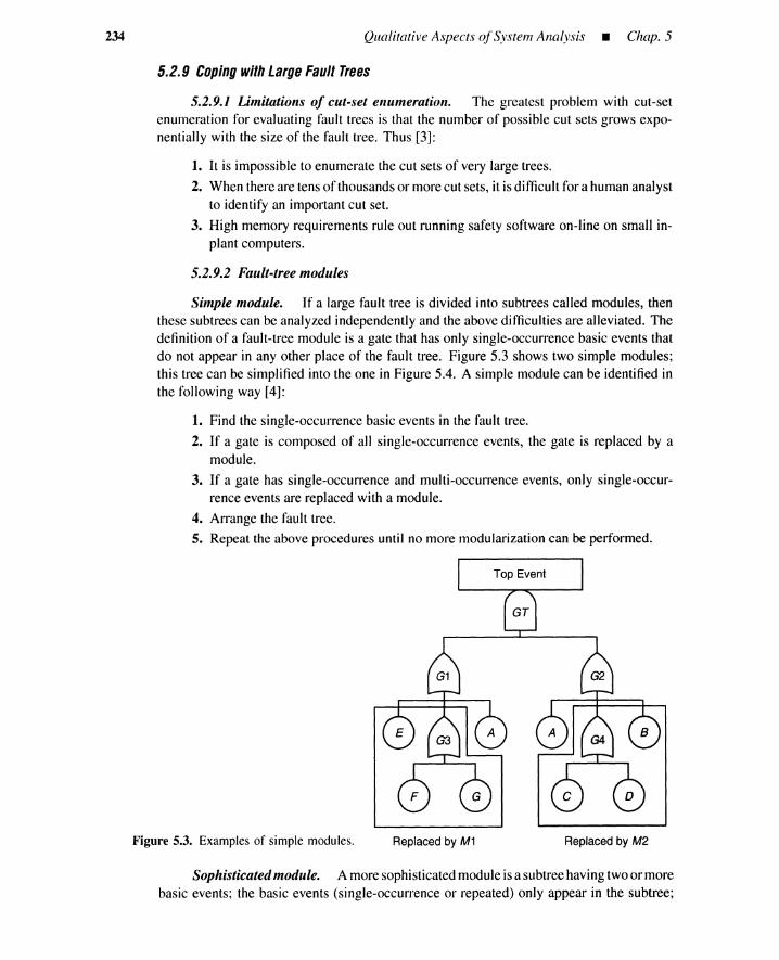
234 Qualitative Aspects ofSystem Analysis • Chap. 5
5.2.9 Coping with Large Fault Trees
5.2.9.1 Limitations of cut-set enumeration. The greatest problem with cut-setenumeration for evaluating fault trees is that the number of possible cut sets grows expo-nentially with the size of the fault tree. Thus [3]:
1. It is impossible to enumerate the cut sets of very large trees.
2. When there are tens of thousands or morecut sets, it isdifficult for a human analystto identify an important cut set.
3. High memory requirements rule out running safety software on-line on small in-plant computers.
5.2.9.2 Fault-tree modules
Simple module. If a large fault tree is divided into subtrees called modules, thenthese subtrees can be analyzed independently and the above difficulties are alleviated. Thedefinition of a fault-tree module is a gate that has only single-occurrence basic events thatdo not appear in any other place of the fault tree. Figure 5.3 shows two simple modules;this tree can be simplified into the one in Figure 5.4. A simple module can be identified inthe following way [4]:
1. Find the single-occurrence basic events in the fault tree.
2. If a gate is composed of all single-occurrence events, the gate is replaced by amodule.
3. If a gate has single-occurrence and multi-occurrence events, only single-occur-rence events are replaced with a module.
4. Arrange the fault tree.5. Repeat the above procedures until no more modularization can be performed.
Figure 5.3. Examples of simple modules. Replaced by M1 Replaced by M2
Sophisticated module. A moresophisticatedmodule isa subtreehavingtwoor morebasic events; the basic events (single-occurrence or repeated) only appear in the subtree;
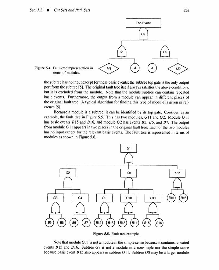
Sec. 5.2 • Cut Sets and Path Sets
Figure 5.4. Fault-tree representation interms of modules.
235
the subtree has no input except for these basic events; the subtree top gate is the only outputport from the subtree [5]. The original fault tree itself always satisfies the above conditions,but it is excluded from the module. Note that the module subtree can contain repeatedbasic events. Furthermore, the output from a module can appear in different places ofthe original fault tree. A typical algorithm for finding this type of module is given in ref-erence [5].
Because a module is a subtree, it can be identified by its top gate. Consider, as anexample, the fault tree in Figure 5.5. This has two modules, G 11 and G2. Module GIlhas basic events B 15 and B 16, and module G2 has events B5, B6, and B7. The outputfrom module GIl appears in two places in the original fault tree. Each of the two moduleshas no input except for the relevant basic events. The fault tree is represented in terms ofmodules as shown in Figure 5.6.
Figure 5.5. Fault-tree example.
Note that module GIl is not a module in the simple sense because it contains repeatedevents B 15 and B 16. Subtree G8 is not a module in a nonsimple nor the simple sensebecause basic event B 15 also appears in subtree GIl. Subtree G8 may be a larger module
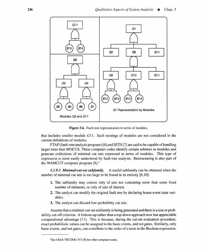
236 Qualitative Aspects ofSystem Analysis _ Chap. 5
G1 Representation by Modules
Modules G2 and G11
Figure 5.6. Fault-treerepresentation in terms of modules.
that includes smaller module G II. Such nestings of modules are not considered in thecurrent definitions of modules.
FTAP(fault-treeanalysis program) [6]and SETS [7]are said to becapable of handlinglarger trees than MOCUS. These computer codes identify certain subtrees as modules andgenerate collections of minimal cut sets expressed in terms of modules. This type ofexpression is more easily understood by fault-tree analysts. Restructuring is also part ofthe WAMCUTcomputer program [8].*
5.2.9.3 Minimal-cut-set subfamily. A useful subfamily can be obtained when thenumber of minimal cut sets is too large to be found in its entirety [6,10]:
1. The subfamily may consist only of sets not containing more than some fixednumber of elements, or only of sets of interest.
2. The analyst can modify the original fault tree by declaring house event state vari-ables.
3. The analyst can discard low-probability cut sets.
Assume that a minimal-cut-setsubfamily is beinggenerated and there is a size or prob-ability cut-off criterion. A bottom-up rather than a top-downapproach now has appreciablecomputational advantage [II]. This is because, during the cut-set evaluation procedure,exact probabilistic valuescan be assigned to the basic events, and not gates. Similarly,onlybasic events, and not gates, can contribute to the order of a term in the Boolean expression.
*See IAEA-TECDOC-553 [9] for other computer codes.

Sec. 5.2 • Cut Sets and Path Sets 237
In the case of the top-down approach, at an intermediate stage of computation, the Booleanexpression for the top gate contains mostly gates and so very few terms can be discarded.The Boolean expression can contain a prohibitive number of terms before the basic eventsare even reached and the cut-off procedure applied. In the bottom-up approach, the Booleanexpression contains only basic events and the cut-off can be applied immediately.
5.2.9.4 MOCUS improvement. The MOCUS algorithm can be improved by gatedevelopment procedures such as FATRAM (fault-tree reduction algorithm) [12]. OR gateswith only basic-event inputs are called basic-event OR gates. These gates are treateddifferently from other gates. Repeated events and nonrepeated events in the basic-event ORgates are processed differently:
1. Rule 1: The basic-event OR gates are not developed until all OR gates with oneor more gate inputs and all AND gates with any inputs are resolved.
2. Rule 2: Remove any supersets before developing the basic-event OR gates.
3. Rule 3: First process repeated basic events remaining in the basic-event OR gates.For each repeated event do the following:(a) Replace the relevant basic-event OR gates by the repeated event, creating
additional sets.(b) Remove the repeated event from the input list of the relevant basic-event OR
gates.(c) Remove supersets.
4. Rule 4: Develop the remaining basic-event OR gates without any repeated events.
All sets become minimal cut sets without any superset examinations.FATRAM can be modified to cope with a situation where only minimal cut sets up to
a certain order are required [12].
Example 7-FATRAM. Consider the fault tree in Figure 5.7. The top event is an ANDgate. The fault tree contains two repeated events, Band C. The top gate is an AND gate, and weobtain by MOCUS:
GI,G2
Gate G I is an AND gate. Thus by Rule I, it can be resolved to yield:
A,G3,G2
Both G3 and G2 are OR gates, but G3 is a basic-event OR gate. Therefore, G2 is developednext (Rule 1) to yield:
A,G3,BA,G3,E
A,G3,G4
G4 is an AND gate and is the next gate to be developed (Rule 1):
A,G3,BA,G3,E
A,G3,D,G5
The gates that remain, G3 and G5, are both basic-event OR gates. No supersets exist (Rule 2), sorepeated events (Rule 3) are handled next.

238 Qualitative Aspects ofSystem Analysis • Chap. 5
Figure 5.7. Example fault tree forMOCUS improvement.
Consider basic event B, which is input to gates G2 and G3. G2 has already been resolved butG3 has not. Everywhere G3 occurs in the sets it is replaced by B, thus creating additional sets:
A,G3,B
A,B,B~ A,B
A,G3,E
A,B,E
A,G3,D,G5
A,B,D,G5
Gate G3 (Rule 3-b) is altered by removing B as an input. Hence, G3 is now an OR gate withtwo basic-event inputs, C and H. Supersets are deleted (Rule 3-c):
A,B
A,G3,E
A,G3,D,G5
Basic event C is also a repeated event; it is an input to G3 and G5. By Rule 3-a replace G3and G5 by C, thus creating additional sets:
A,B
A,G3,E
A,C,E
A,G3,D,G5
A,C,D,C~ A,C,D
Gate G3 now has only input H, and G5 has inputs F and G. Supersets are removed at thispoint (Rule 3-c) but none exist and all repeated events have been handled. We proceed to Rule 4, toobtain all minimal cut sets:

Sec. 5.2 • Cut Sets and Path Sets 239
A,B
A,H,EA,C,E
A,H,D,FA,H,D,G
A,C,D
•Example 8-Boolean explanation ofFATRAM. The above procedure for developing
gates can be written in matrix form.
I TI = IGI I G21 = IA I G3 I G21 = IA I G3 B = IA I G3E
G4
BED I G5
(5.19)
Denote by X a Booleanexpression. The following identities hold:
X . A = (XIA = true) . A
X . A = (XIA = false) . A(5.20)
(5.21)
When expression X has no complement variables, then for Boolean variables A and B
A . X + B . X = A . (XIA = true) + B . (XIA = false)
Applying (5.22) to (5.19) with repeated event B as a condition,
T=IAI B B =IAIBG3 E G31E
D I G5 D I G5
Applying (5.22) with repeated event C as a condition,
(5.22)
(5.23)
(5.24)I~=IA B
CB
C IEG3 Die
G5
G31ED I G5
Replace G3 by Hand G5 by F and G to obtain all minimal cut sets:
T=IA B
CI~I(5.25)
HIEDI~
•5.2.9.5 Set comparison improvement. It can be proven that neither superset re-
moval by absorption x + xy = x nor simplification by idempotence xx = x is requiredwhen a fault tree does not contain repeated events [13]. The minimal cut sets are thoseobtained by a simple development using MOCUS. When repeated events appear in fault
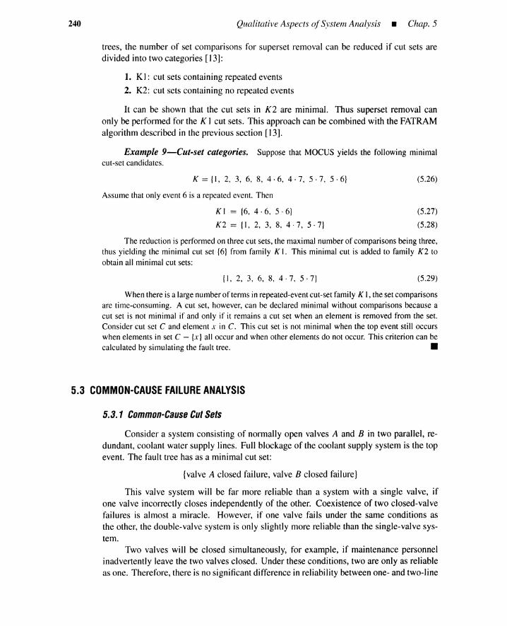
240 Qualitative Aspects ofSystem Analysis _ Chap. 5
trees, the number of set comparisons for superset removal can be reduced if cut sets aredivided into two categories [13]:
1. K1: cut sets containing repeated events
2. K2: cut sets containing no repeated events
It can be shown that the cut sets in K2 are minimal. Thus superset removal canonly be performed for the K I cut sets. This approach can be combined with the FATRAMalgorithm described in the previous section [13].
Example 9-Cut-set categories. Suppose that MOCUS yields the following minimalcut-set candidates.
K = {I, 2, 3, 6, 8, 4·6, 4·7, 5·7, 5· 6}
Assume that only event 6 is a repeatedevent. Then
K I = {6, 4·6, 5· 6}
K2 = {I, 2, 3, 8,4·7, 5·7}
(5.26)
(5.27)
(5.28)
The reductionis performedon three cut sets, the maximalnumberof comparisonsbeing three,thus yielding the minimal cut set {6} from family K I. This minimal cut is added to family K2 toobtain all minimal cut sets:
{I, 2, 3, 6, 8,4·7, 5·7} (5.29)
Whenthere is a largenumberof terms in repeated-event cut-set family K 1,the set comparisonsare time-consuming. A cut set, however, can be declared minimal without comparisons because acut set is not minimal if and only if it remains a cut set when an element is removed from the set.Consider cut set C and element x in C. This cut set is not minimal when the top event still occurswhen elements in set C - {x} all occur and when other elements do not occur. This criterion can becalculated by simulating the fault tree. •
5.3 COMMON-CAUSE FAILURE ANALYSIS
5.3.1 Common-Cause Cut Sets
Consider a system consisting of normally open valves A and B in two parallel, re-dundant, coolant water supply lines. Full blockage of the coolant supply system is the topevent. The fault tree has as a minimal cut set:
{valve A closed failure, valve B closed failure}
This valve system will be far more reliable than a system with a single valve, ifone valve incorrectly closes independently of the other. Coexistence of two closed-valvefailures is almost a miracle. However, if one valve fails under the same conditions asthe other, the double-valve system is only slightly more reliable than the single-valve sys-tem.
Two valves will be closed simultaneously, for example, if maintenance personnelinadvertently leave the two valves closed. Under these conditions, two are only as reliableas one. Therefore, there is no significantdifference in reliability between one- and two-line

Sec. 5.3 • Common-Cause Failure Analysis 241
systems. A condition or event that causes multiple basic events is called a common cause.An example of a common cause is a flood that causes all supposedly redundant componentsto fail simultaneously.
The minimal-cut-generation methods discussed in the previous sections give minimalcuts of various sizes. A cut set consisting of n basic events is called an n-event cut set.One-event cut sets are significant contributors to the top event unless their probability ofoccurrence is very small. Generally, hardware failures occur with low frequencies; hence,two-or-more-event cut sets can often be neglected if one-event sets are present becauseco-occurrence of rare events have extremely low probabilities. However, when a commoncause is involved, it may cause multiple basic-event failures, so we cannot always neglecthigher order cut sets because some two-or-more-event cut sets may behave like one-eventcut sets.
A cut set is called a common-cause cut set when a common cause results in theco-occurrence of all events in the cut set. Taylor reported on the frequency of commoncauses in the U.S. power reactor industry [14]: "Of 379 component failures or groupsof failures arising from independent causes, 78 involved common causes." In system-failure-mode analysis, it is therefore very important to identify all common-cause cutsets.
5.3.2 Common Causes and Basic Events
As shown in Figure 4.16, causes creating component failures come from one or moreof the following four sources: aging, plant personnel, system environment, and systemcomponents (or subsystems).
There are a large number of common causes in each source category, and these canbe further classified into subcategories. For example, the causes "water hammer" and "pipewhip" in a piping subsystem can be put into the category "impact." Some categories andexamples are listed in Table 5.1 [15].
For each common cause, the basic events affected must be identified. To do this,a domain for each common cause, as well as the physical location of the basic eventand component must be identified. Some common causes have only limited domainsof influence, and the basic events located outside the domain are not affected by thecauses. A liquid spill may be confined to one room, so electric components will notbe damaged by the spill if they are in another room and no conduit exists between thetwo rooms. Basic events caused by a common cause are common-cause events of thecause.
Consider the fault tree of Figure 5.8. The floor plan is shown in Figure 5.9. Thisfigure also includes the location of the basic events. We consider 20 common causes. Eachcommon cause has the set of common-cause events shown in Table 5.2. This table alsoshows the domain of each common cause.
Only two basic events, 6 and 3, are caused by impact 11, whereas basic events 1,2,7,8are caused by impact 12. This difference arises because each impact has its own domainof influence, and each basic event has its own location of occurrence. Neither event 4 norevent 12 are caused by impact 11 although they are located in domain 104 of 11. Thisis because these events occur independently of the impact, although they share the samephysical location as event 3; in other words, neither event 4 nor 12 are susceptible toimpact II.

242 Qualitative Aspects ofSystem Analysis - Chap. 5
TABLE 5.1. Categories and Examples of Common Causes
Source Symbol Category Examples
Environment, I Impact Pipe whip, water hammer, missiles,System, earthquake, structuralfailureComponents, V Vibration Machineryin motion,earthquakeSubsystems P Pressure Explosion, out-of-tolerance system changes
(pump overspeed, flow blockage)G Grit Airborne dust, metal fragments generated by
moving parts with inadequate tolerancesS Stress Thermal stress at welds of dissimilar
metals, thermal stresses and bendingmoments caused by high conductivity anddensity
T Temperature Fire, lightning, weld equipment,cooling-system fault, electrical shortcircuits
E Loss of energy Common drive shaft, same powersource supply
C Calibration Misprinted calibrationinstructionF Manufacturer Repeated fabrication error, such as neglect to
properly coat relay contacts. Poor work-manship. Damage during transportation
Plant IN Installation Same subcontractor or crewPersonnel contractor
M Maintenance Incorrect procedure, inadequately trainedpersonnel
0 Operation Operator disabled or overstressed, faultyoperating procedures
TS Test Fault test procedures that may affect allcomponents normally tested together
Aging A Aging Components of same materials
5.3.3 Obtaining Common-Cause Cut Sets
Assume a list of common causes, common-causeevents, and basic events. Common-cause cut sets are readily obtained if all the minimalcut sets of a given fault tree are known.Large fault trees, however, may have an astronomically large number of minimal cut sets,and it is time-consuming to obtain them. For such fault trees, the generation methodsdiscussed in the previous sections are frequently truncated to give, for instance, only two-or-less-eventcut sets. However, this truncationshouldnot be usedwhenthere is a possibilityof common-cause failures because three-or-more-event cut sets may behave like one-eventcut sets and hence should not be neglected.
One approach, due to Wagner et al. [15] is based on dissection of fault trees. Analternative method using a simplified fault tree is developed here.
A basic event is called a neutral event vis-a-vis a common cause if it is independentof the cause. For a given common cause, a basic event is thus either a neutral event or acommon-causeevent. The present approachassumesa probable situation for each common

Sec. 5.3 • Common-Cause Failure Analysis
Figure 5.8. Fault tree for the exampleproblem.
102 104
00 0 8 0)199
106
G103
0 G101 105 0
8 00Figure 5.9. Examplefloorplan and locationof basic events.
243
cause. This situation is defined by the statement: "Assume a common cause. Because mostneutral events have far smaller possibilities of occurrence than common-cause events, theseneutral events are assumed not to occur in the given fault tree." Other situations violatingthe above requirement can be neglected because they imply the occurrence of one or moreneutral events.
The probable-situation simplifies the fault tree. It uses the fundamental simplificationof Figure 5.10 in a bottom-up fashion. For the simplified fault tree, we can easily obtain theminimal cut sets. These minimal cut sets automatically become the common-cause cut sets.
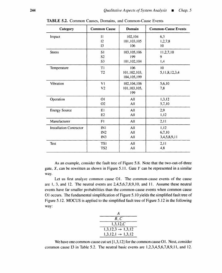
244 Qualitative Aspects of System Analysis _ Chap. 5
TABLE 5.2. Common Causes, Domains, and Common-Cause Events
Category Common Cause Domain Common-Cause Events
Impact II 102,104 6,312 101,103,105 1,2,7,813 106 10
Stress SI 103,105,106 11,2,7,10S2 199 9S3 101,102,104 1,4
Temperature TI 106 10T2 101,102,103, 5, II ,8,12,3,4
104,105,199
Vibration VI 102,104,I06 5,6,10V2 101,103,105, 7,8
199
Operation 01 All 1,3,1202 All 5,7,10
Energy Source EI All 2,9E2 All 1,12
Manufacturer FI All 2,11
Installation Contractor INI All 1,12IN2 All 6,7,10IN3 All 3,4,5,8,9,II
Test TSI All 2,11TS2 All 4,8
As an example, consider the fault tree of Figure 5.8. Note that the two-out-of-three
gate, X, can be rewritten as shown in Figure 5.11. Gate Y can be represented in a similarway.
Let us first analyze common cause 01. The common-cause events of the causeare 1,3, and 12. The neutral events are 2,4,5,6,7,8,9,10, and 11. Assume these neutral
events have far smaller probabilities than the common-cause events when common cause
01 occurs. The fundamental simplification of Figure 5.10 yields the simplified fault tree of
Figure 5.12. MOCUS is applied to the simplified fault tree of Figure 5.12 in the following
way:
A
B,C1,3,12,C
1,3,12,3 ~ 1,3,121,3,12,1 ~ 1,3,12
We have one common-cause cut set {1,3, 12}for the common cause 01. Next, consider
common cause 13 in Table 5.2. The neutral basic events are 1,2,3,4,5,6,7,8,9,11, and 12.
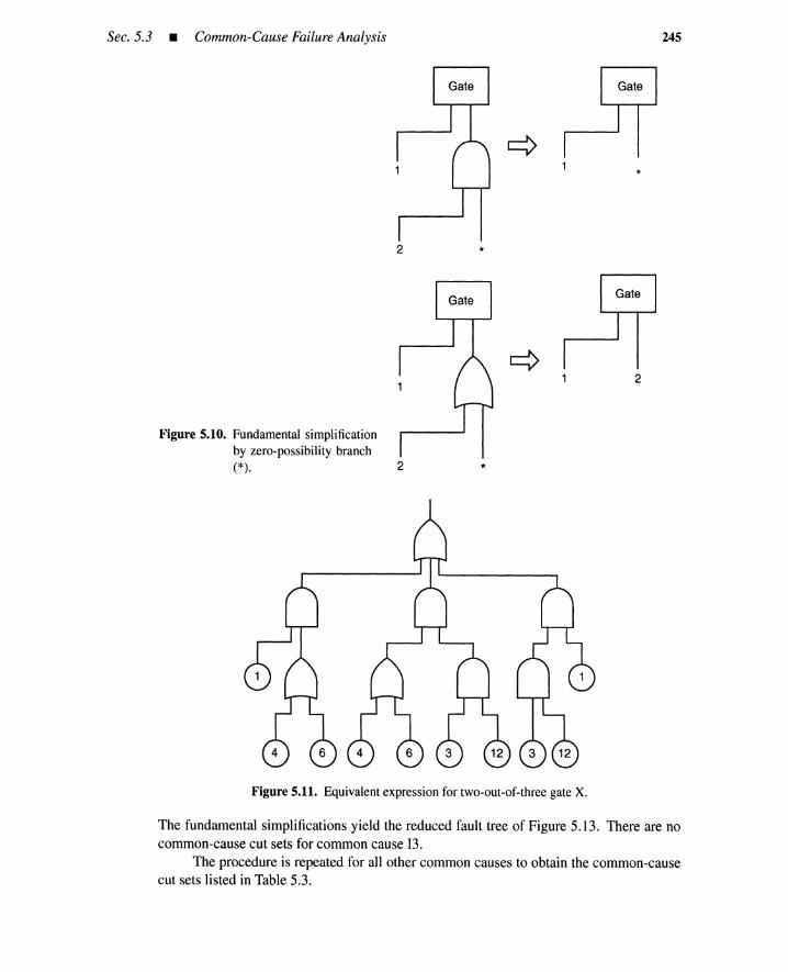
Sec. 5.3 • Common-Cause Failure Analysis 245
2
Figure 5.10. Fundamental simplificationby zero-possibility branch(*). 2
*
*
2
Figure 5.11. Equivalent expressionfor two-out-of-three gate X.
The fundamental simplifications yield the reduced fault tree of Figure 5.13. There are nocommon-cause cut sets for common cause 13.
The procedure is repeated for all other common causes to obtain the common-causecut sets listed in Table 5.3.

246 Qualitative Aspects ofSystem Analysis • Chap. 5
Figure 5.12. Simplified fault tree forcommon cause a I.
Zero Possibility
Figure 5.13. Simplified fault tree forcommon cause 13.
TABLE 5.3. Common Causes and Common-Cause Cut Sets
Common Cause
1212S3SIT201
Common-Cause Cut Set
{1,2}{1,7,8}{1,4}{2,10,11}{3,4,12}{1,3,12}
5.4 FAULT·TREE LINKING ALONG AN ACCIDENT SEQUENCE
5.4.1 Simple Example
Consider an event tree in Figure 5.14. Event-tree-failureheadings are represented by the faulttrees in Figure 5.15. Consider two families of minimal cut sets for accident sequence 52 and 54 [16].Other sequences are treated in a similar way.
5.4.1.1 Cut sets for event-tree headings. Denote by Fl failureof system I (Fig. 5.15).The minimal cut sets for this failure are:
FI=C+F+A·B+D·E
Similarly, failure F2 of system 2 can be expressed as:
F2 = A + F + G
(5.30)
(5.31)
•5.4.1.2 Cut sets for sequence 2. In the second sequence 52, system I functions while
system 2 is failed. Thus this sequence can be represented as:
52 = Fl· F2 (5.32)
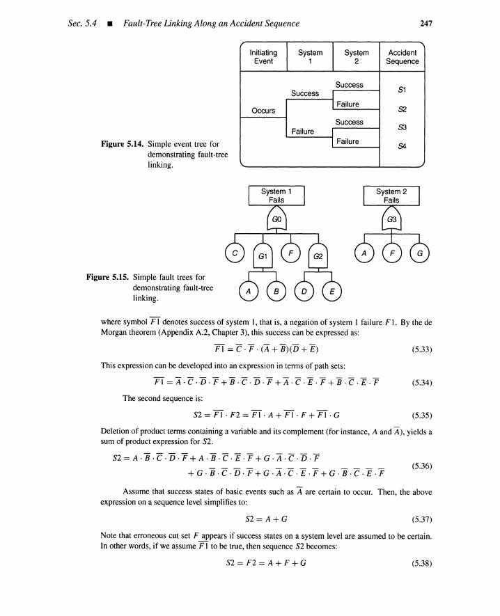
Sec. 5.4 • Fault-Tree Linking Along an Accident Sequence 247
Figure 5.14. Simple event tree fordemonstrating fault-treelinking.
"Initiating System System AccidentEvent 1 2 Sequence
Success51Success
FailureS2Occurs
Success53Failure
Failure54
Figure 5.15. Simple fault trees fordemonstrating fault-treelinking.
where symbol FT denotes success of system 1, that is, a negation of system 1 failure F I. By the deMorgan theorem (Appendix A.2, Chapter 3), this success can be expressed as:
FT= C.F . (X + Ii)(i5+E) (5.33)
This expression can be developed into an expression in terms of path sets:
FT = A .C .D .F +B .C .D .F + A .C .E .F + B .C .E .F (5.34)
The second sequence is:
S2 = FT. F2 =FT. A + FT . F +FT. G (5.35)
Deletion of product terms containing a variable and its complement (for instance, A and A), yields asum of product expression for S2.
S2 = A·Ii·c·[j ·F+A· Ii· C· E ·F+G· A·c·[j·F
+ G· Ii· c· [j. F+ G· A·C· E· F+G· Ii·c· E· F(5.36)
Assume that success states of basic events such as A are certain to occur. Then, the aboveexpression on a sequence level simplifies to:
S2=A+G (5.37)
Note that erroneous cut set F appears if success states on a system level are assumed to be certain.In other words, if we assume FT to be true, then sequence S2 becomes:
S2 = F2 = A + F + G (5.38)

248 Qualitative Aspects ofSystem Analysis _ Chap. 5
Negationsof events appear in equation (5.36) because sequence 2 contains the system successstate, that is, FT. Generally, a procedure for obtaining prime implicants must be followed for enu-merationof minimalcut sets containing success events. Simplificationstypifiedby the followingruleare required, and this is a complication (see Section 5.5).
AB+AB=A (5.39)
Fortunately, it can be shown that the following simplificationrules are sufficientfor obtainingthe accident-sequence minimal cut sets involvingcomponent success states if the original fault treescontain no success events. Note that success events are not included in fault trees F I or F2:
A2 = A, (Idempotent)
AB + AB = AB, (Idempotent)
A + AB = A, (Absorption)
A . A = false, (Complementation)
(5.40)
(5.41)
(5.42)
(5.43)
•5.4.1.3 Cut sets for sequence 4. In sequence 54, both systems fail and the sequence cut
sets are obtained by a conjunction of system I and 2 cut sets.
54 = Fl· F2 = FI . (A + F + G)
= Fl· A + Fl· F + Fl· G(5.44)
A manipulationbasedon equation(5.20) is simpler than thedirectexpansionof equation (5.44):
54 = (F IIA = true) . A + (F IIF = true) . F + (F IIG = true) . G
= (C + F + B + D . E) . A + (true) . F + (C + F + A . B + D . E) . G
= F + (C + F + B + D . E) . A + (C + F + A . B + D . E) . G
(5.45)
Minimal cut F consists of only one variable. It is obvious that all cut sets of the form F . Pwhere P is a product of Boolean variablescan be deleted from the second and the third expressionsof equation (5.45).
54 = F + (C + B + D . E) . A + (C + A . B + D . E) . G
This expression is now expanded:
54 = F + A . C + A . B + A . D . E + C . G + A . B . G + D . E . G
(5.46)
(5.47)
Cut set A . B . G is a superset of A . B, thus the family of minimal cut sets for sequence 54 is:
54 = F + A . C + A . B + A . D . E + C . G + D . E . G
5.4.2 AMore Realistic Example
(5.48)
•For the swimming pool reactor of Figure 4.46 and its event tree of Figure 4.48, consider the
minimal cut sets for sequence 53 consisting of a trip system failure and an isolation system success.The two event headings are represented by the fault trees in Figures4.49 and 4.51, and Table5.4 liststheir basic events. Events I through 6 appear only in the trip-system-failurefault tree, as indicated bysymbol "Yes" in the fourth column; events 101 and 102 appear only in the isolation-system-failurefault tree; events 11 through 17 appear in both fault trees. Since the two fault trees have commonevents, the minimal cut sets of accident sequence 53 must be enumerated accordingly. Table 5.4also shows event labels in the second column where symbols P, Z, and FO denote "Positive outputfailure," "Zero output failure," and "Fully.Open failure," respectively. Characters following each of

Sec. 5.4 • Fault-Tree Linking Along an Accident Sequence
TABLE 5.4. Basic Events of the Two Fault Trees Along an AccidentSequence
Event Label Description Trip Isolation
1 ZNAND Zero output failureof NANDgate Yes No2 PC5 Positiveoutput failureof C5 Yes No3 PC6 Positiveoutput failureof C6 Yes No4 PC7 Positiveoutput failureof C7 Yes No5 PC8 Positiveoutput failure of C8 Yes No6 PC14 Positiveoutput failureof C14 Yes No
11 ZC3 Zero output failureof C3 Yes Yes12 ZC4 Zero output failure of C4 Yes Yes13 FOC9 Fully.Open failure of C9 Yes Yes14 FOCIO Fully.Open failure of C10 Yes Yes15 ZCll Zero output failureof C11 Yes Yes16 PC12 Positiveoutput failure of C12 Yes Yes17 ZC13 Zero output failureof C13 Yes Yes
101 FOCI Fully.Open failure of C1 No Yes102 FOC2 Fully.Open failure of C2 No Yes
249
these symbolsdenote a relevantcomponent; for instance,ZC11 for event 15implies that componentC11 has a "Zero output failure." •
5.4.2.1 Trip system failure. The trip system failure is represented by the fault tree inFigure4.49, which has four nested modules,RSM54, RSM18,RM40, RM92, and RM34. Inclusionrelations are shown in Figure 4.50. Modules RSM54 and RSM18 are the most elementary; moduleRM40includesmodulesRSM54and RSMI8; modulesRM92 and RM34 contain moduleRM40.
Denote by T the top event of the fault tree, whichcan be representedas:
T = (M18 + 6)(M34 + 4)(M34 + 5)(M92 + 2)(M92 + 3)M54 + 1 (5.49)
where symbol M 18, for example, representsa top event for moduleRSM18.The following identity is used to expand the aboveexpression.
(A + X)(A + Y) = A + XY (5.50)
where A, X, and Y are any Boolean expressions. In equation (5.49), M34 and M92 correspond tocommonexpression A. Topevent T can be writtenas:
T = (M18 + 6)(M34 + 4· 5)(M92 + 2· 3)M54 + 1
Modules34 and 92 are expressedin terms of module40:
(5.51)
T = (M18 + 6)(M40 + 12+ 4· 5)(M40 + 11 + 2· 3)M54 + 1 (5.52)
Applyingequation (5.50) for A == M40:
T = (M18 + 6)[M40 + (12+ 4·5)(11 + 2· 3)]M54 + 1
Module40 is expressedin terms of modules 18and 54:
(5.53)
T = (M18 + 6)[(MI8 + 14)(M54 + 13)+ (12 + 4·5)(11 + 2· 3)]M54 + 1 (5.54)
Applyingequation (5.20) for A == M54:
T = (M18 + 6)[MI8 + 14+ (12 + 4·5)(11 + 2· 3)]M54 + 1 (5.55)
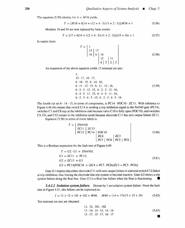
250 QualitativeAspects ofSystem Analysis • Chap. 5
The equation (5.50) identity for A = M 18yields:
T = {MI8+6[14+(12+4·5)(11 +2·3)]}M54+ I
Modules 18and 54 are now replaced by basic events:
T = {17+6[14+ (12+4·5)(11 +2·3)]}(15+ 16)+ I
In matrix form:
T= I15
1
1716 6 14
12 III415 21 3
An expansion of the above equation yields 13 minimal cut sets:
I,15·17, 16·17,6·14·15,6·14·16,6 . II . 12 . 15, 6· II . 12 . 16,6·2·3 ·12·15,6·2·3·12·16,6·4·5·11·15,6·4·5·11·16,6·2·3·4·5·15,6·2·3·4·5·16
(5.56)
(5.57)
(5.58)
(5.59)
(5.60)
The fourth cut set 6·14·15, in terms of components, is PCI4· FaCIO· ZCIl. With reference toFigure 4.46 this means that switch CI4 is sending a trip inhibition signal to the NAND gate (PCI4),switches C7 and C8 stay at the inhibition side because valveC lOis fully open (FOC10),and switchesC5, C6, and C12remain in the inhibition mode because electrode C II has zero output failure ZCII.
Equation (5.58) in terms of event labels is:
T = ZNAND
ZCII I ZCI3PCI2 PCI4 FOCIO
ZC4 IZC3PC7 I PC8 PC5 I PC6
This is a Boolean expression for the fault tree of Figure 4.49:
T = G2 . G I + ZNAND,
GI = ZCII + PCI2,
G2=ZCI3 +G3
G3 = PCI4[FOCIO + (ZC4 + PC7 . PC8)(ZC3 + PC5 . PC6)]
(5.61)
Gate G I implies thateither electrodeC II with zero output failureor solenoidswitchC12failedat trip inhibition, thus forcing the electrode line trip system to become inactive. Gate G2 shows a tripsystem failure along the float line. Gate G3 is a float line failure when the float is functioning. •
5.4.2.2 Isolation systemfailure. Denote by I an isolation system failure. From the faulttree in Figure 4.51, this failure can be expressed as:
I = 11+ 12+ 101 + 102+ M40, M40 = (14 + 17)(13 + 15 + 16) (5.62)
Ten minimal cut sets are obtained:
II, 12, 101, 10213. 14, 14· 15, 14· 1613·17, 15·17, 16· 17
(5.63)
•
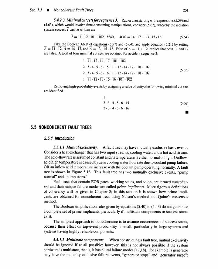
Sec. 5.5 • Noncoherent Fault Trees 251
5.4.2.3 Minimal cutsetsfor sequence 3. Ratherthanstartingwithexpressions (5.59)and(5.63), which would involve time-consuming manipulations, consider (5.62), whereby the isolationsystemsuccessI can be writtenas:
I = TI· 12·TOT· 102· M40, M40 =14·17 +13·15·16 (5.64)
Take the Boolean AND of equations (5.57) and (5.64), and apply equation (5.21) by settingA = IT·12, A == 14 ·17, and A = 13·15·16. False of A = II + 12 implies that both 11 and 12are false. A total of four minimal cut sets are obtainedfor accidentsequence3:
1 . TI ·12· 14·17· TOT· 102
2·3·4·5·6· I5·TI·T2·14·T7·TOT· 102
2·3·4·5·6· 16·TI·12·14·T7·TOT· 102
1 . IT .12 . T3 .15 .16 .TOT . 102
(5.65)
Removing high-probability eventsby assigning a valueof unity, the following minimal cut setsare identified.
5.5 NONCOHERENT FAULT TREES
5.5.1 Introduction
1
2·3·4·5·6·15
2·3·4·5·6·16(5.66)
•
5.5.1.1 Mutual exclusivity. A fault tree may have mutually exclusive basic events.Consider a heat exchanger that has two input streams, cooling water, and a hot acid stream.The acid-flow rate is assumed constant and its temperature is either normal or high. Outflow-acid high temperature is caused by zero cooling water flow rate due to coolant pump failure,OR an inflow acid temperature increase with the coolant pump operating normally. A faulttree is shown in Figure 5.16. This fault tree has two mutually exclusive events, "pumpnormal" and "pump stops."
Fault trees that contain EOR gates, working states, and so on, are termed noncoher-ent and their unique failure modes are called prime implicants. More rigorous definitionsof coherency will be given in Chapter 8; in this section it is shown how prime impli-cants are obtained for noncoherent trees using Nelson's method and Quine's consensusmethod.
The Boolean simplification rules given by equations (5.40) to (5.43) do not guaranteea complete set of prime implicants, particularly if multistate components or success statesexist.
The simplest approach to noncoherence is to assume occurrences of success states,because their effect on top-event probability is small, particularly in large systems andsystems having highly reliable components.
5.5.1.2 Multistate components. When constructing a fault tree, mutual exclusivityshould be ignored if at all possible; however, this is not always possible if the systemhardware is multistate, that is, it has plural failure modes [17,18]. For example, a generatormay have the mutually exclusive failure events, "generator stops" and "generator surge";

252 Qualitative Aspects ofSystem Analysis • Chap. 5
HighTemperatureof Outflow
Acid
NormalCoolingWater Flow
Rate toHeat Exchanger
NormalCoolingWaterPressure to Valve
2
Zero CoolingWaterFlow Rate to
Heat Exchanger
Zero CoolingWaterPressure to
Valve
3
Figure 5.16. Fault tree for heatexchanger.
a relay may be "shorted" or remain "stuck open," and a pump may, at times, be a four-state component: state I-no flow; state 2-flow equal to one third of full capacity; state3-flow at least equal to two thirds of, but less than, full capacity; state 4-pump fullyoperational.
5.5.2 Minimal Cut Sets for a Binary Fault Tree
When a fault tree contains mutually exclusive binary events, the MOCUS algorithmdoes not always produce the COITect minimal cut sets. MOCUS, when applied to the tree ofFigure 5.16, for example, yields the cut sets {I ,2} and {3}. Thus minimal cut set {I} cannotbe obtained by MOCUS, although it would be apparent to an engineer, and numerically,the probability of {I} and {I ,2} is the same for all practical purposes.
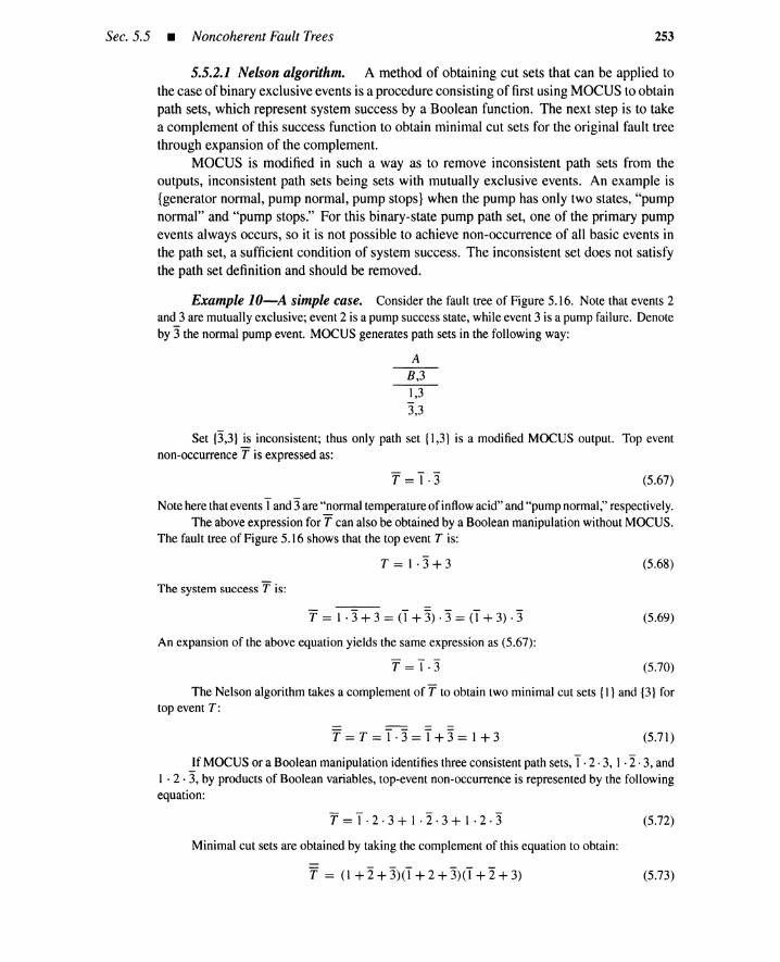
Sec. 5.5 • Noncoherent FaultTrees 253
5.5.2.1 Nelson algorithm. A method of obtaining cut sets that can be applied tothecase of binaryexclusive eventsis a procedureconsistingof firstusingMOCUSto obtainpath sets, which represent system success by a Boolean function. The next step is to takea complementof this success function to obtain minimal cut sets for the original fault treethroughexpansionof the complement.
MOCUS is modified in such a way as to remove inconsistent path sets from theoutputs, inconsistentpath sets being sets with mutually exclusive events. An example is{generator normal,pump normal, pump stops} when the pump has only two states, "pumpnormal" and "pump stops." For this binary-state pump path set, one of the primary pumpevents always occurs, so it is not possible to achieve non-occurrence of all basic events inthe path set, a sufficient conditionof system success. The inconsistentset does not satisfythe path set definition and should be removed.
Example lO-A simple case. Consider the fault tree of Figure 5.16. Note that events 2and 3 are mutuallyexclusive; event2 is a pump successstate,whileevent3 is a pumpfailure. Denoteby3 the normalpump event. MOCUSgeneratespath sets in the following way:
AB,31,3
3,3
Set {3,3} is inconsistent; thus only path set {1,3} is a modified MOCUS output. Top eventnon-occurrence T is expressedas:
T = 1· 3 (5.67)
Noteherethatevents1and3are"normaltemperatureof inflowacid"and"pumpnormal," respectively.The aboveexpressionforT can also be obtainedby a Booleanmanipulation withoutMOCUS.
The fault tree of Figure 5.16 shows that the top event Tis:
T=I·3+3
The system success Tis:
T = 1 ·3+ 3 = (1+ 3)·3= (1+ 3) ·3
An expansionof the aboveequation yields the same expression as (5.67):
T= 1·3
(5.68)
(5.69)
(5.70)
The Nelsonalgorithmtakes a complementofT to obtain two minimalcut sets {I} and {3} fortop event T:
(5.71)
If MOCUSor a Booleanmanipulation identifies threeconsistentpath sets,1.2 . 3, I ·2·3, and1 . 2 . 3, by productsof Boolean variables, top-eventnon-occurrence is represented by the followingequation:
T=I·2·3+1·2·3+1·2.3
Minimalcut sets are obtainedby taking the complementof this equation to obtain:
T = (I + 2: + 3)(1 + 2+ 3)(1 + 2+ 3)
(5.72)
(5.73)
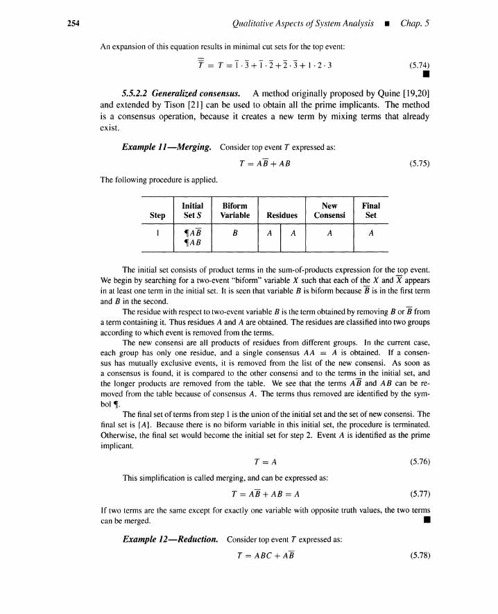
254 Qualitative Aspects ofSystem Analysis • Chap. 5
An expansion of this equation results in minimal cut sets for the top event:
T = T=1·3+1·2+2·3+1·2·3 (5.74)
•5.5.2.2 Generalizedconsensus. A method originally proposed by Quine [19,20]
and extended by Tison [21] can be used to obtain all the prime implicants. The methodis a consensus operation, because it creates a new term by mixing terms that alreadyexist.
Example II-Merging. Consider top event T expressed as:
T = AB+AB
The following procedure is applied.
Initial Biform New FinalStep SetS Variable Residues Consensi Set
I ,AB B A A A A'AB
(5.75)
The initial set consists of product terms in the sum-of-products expression for the top event.We begin by searching for a two-event "biform" variable X such that each of the X and X appearsin at least one term in the initial set. It is seen that variable B is biform becauseB is in the first termand B in the second.
The residue with respect to two-eventvariable B is the term obtained by removing B or Ii froma term containing it. Thus residues A and A are obtained. The residues are classified into two groupsaccording to which event is removed from the terms.
The new consensi are all products of residues from different groups. In the current case,each group has only one residue, and a single consensus AA = A is obtained. If a consen-sus has mutually exclusive events, it is removed from the list of the new consensi. As soon asa consensus is found, it is compared to the other consensi and to the terms in the initial set, andthe longer products are removed from the table. We see that the terms AB and AB can be re-moved from the table because of consensus A. The terms thus removed are identified by the sym-bol ,.
The final set of terms from step 1is the union of the initial set and the set of new consensi. Thefinal set is {A}. Because there is no biform variable in this initial set, the procedure is terminated.Otherwise, the final set would become the initial set for step 2. Event A is identified as the primeimplicant.
T=A
This simplificationis called merging, and can be expressed as:
T=AB+AB=A
(5.76)
(5.77)
If two terms are the same except for exactly one variable with opposite truth values, the two termscan be merged. •
Example I2-Reduction. Consider top event T expressed as:
T=ABC+AB (5.78)

Sec. 5.5 • NoncoherentFault Trees
The consensus procedure is:
Initial Biform New FinalStep SetS Variable Residues Consensi Set
,ABC B AC AC-
1 A ABAB AC
The top event is simplified:
T = ABC + AB = AB + AC
255
(5.79)
This relation is called reduction; if two terms are comparable except for exactly one variable withopposite truth values, the larger of the two terms can be reduced by that variable. •
The simplification operations (absorption, merging, reduction) are applied to the top-event expressions in cycles, until none of them is applicable. The resultant expression isthen no longer reducible when this occurs.
Example 13-Two-step consensus operation. Consider top event T:
T = ABC + ABC + ABC + ABC
The two-step consensus operation is:
Initial Biform New FinalStep SetS Variable Residues Consensi Set
1 ,ABC B AC AC AC AC,ABC AC AC AC AC,ABC,ABC
2 'AC C A A A A,AC
Thus, the top event is:
T=A
(5.80)
(5.81)
•5.5.2.3 Modularization. Because large trees lead to a large number of product-of-
variables terms that must be examined during prime-implicant generation, computationaltimes become prohibitive when all terms are investigated. Two approaches can be used[22].
Removal ofsingletons. Assume that a Boolean variable A is a cut set of top eventT represented by a sum of products of basic events. Such a variable is called a singleton.The following operations to simplify T can be performed.

256 Qualitative Aspects ofSystem Analysis • Chap. 5
1. All terms of the form A P, where P is a product of basic events other than A itself,are deleted by absorption, that is, A + AP == A.
2. All terms of the form AP are replaced by P, that is, A + AP == A + P.
Example 14-Simplification by singletons. Consider, as an example, top event T [22]:
T = Xg + XIg + X21 + X3 XlO + X6 X lO + XlOX13 + X3 X14 + X6 X14
+X13XI4 + XI X2XlO + X2XlOX24 + XI X2 XI4
+X2X14X24 + XI X5 XlO + XI XlOX25 + X5 XlOX24
+XlOX24X25 + XI X5 XI4 + XIXI4 X25 + XSXI4 X24 + XI4 X24X25
+X9X12X16X19X22X23 + XgX12 X16 Xlg X20 X21 + X9XI1X15X19X22X23 (5.82)
+XgXII XI5 Xlg X20 X21 + X9XlOX14X19X20X22X23 + X2X4X7X9X17X19X22X23X25
+X2X4X7XgX17XlgX20X21X25 + Xl X4 X5 X7 X9 X17 X19 X22 X23 X24
+Xl X4 X 5X7 Xg X 17X18X20 X21 X24
+XIX3X 6X 9X 13X 19X20 X 22X23 X 24 + X2 X 3X 5X 6X9 X 13X 19X20 X 22X23 X25
Because Xg, XIg, and X21 are singletons, the above equation becomes:
T = Xg + XIS + X21 + X3 XlO + X6 XlO + XlOX13 + X3X14 + X6 X14
+X13 XI4 + XI X2XlO + X2 XlOX24 + XI X2 X14
+X2X14X24 + XI X5 XlO + XI XlOX25 + X5 XlOX24
+XlOX24X25 + XI X5 XI4 + XI XI4 X25 + X5X14X24 + X14X24X25
+X9X12X16X19XnX23 + X12 X16 X20 + X9XI1X15X19X22X23
+XIIXI5X20 + X9XlOX14Xl9X2oXnX23 + X2X4X7X9X17X19X22X23X25
+X2X4X7X17X20X25 + XlX4X5X7X9X17X19X22X23X24 + XIX4X5X7X17X20X24
+XlX3X6X9X13XI9X2oXnX23X24 +X2X3X5X6X9Xn X19 X2o X22X23 X25
Modularization. Let A and B be two basic events for which:
(5.83)
•
(5.84)
1. All terms that include A also include B
2. Neither term includes AB3. For each term of the form AP, there also exists a term of the form BP
Then AB can be replaced by Y == (AB) or Z == (AB) in each term that includes AB,the term A P is replaced by Y P or Z P, and term B P is deleted. A or B can be unnegatedor negated variables and so modularization involves consideration of each of the pairs AB,AB, AB, or AB.
ABX + AP + BP == (AB)X + (AB)P == YX +YP == ZX + ZP
ABX + AP + BP == (AB)X + (AB)P == YX +YP == ZX + ZP
ABX + AP + BP == (AB)X + (AB)P == YX + YP == ZX + ZP
ABX + AP + BP == (AB)X + (AB)P == YX +YP == ZX + ZP
Modularization replaces two basic events by one, and can be repeated for all possibleparings of basic events, so that modularizing a group such as A I B I A2 B2 is possible.
Example 15-A modularization process. Consider equation (5.83). All terms thatinclude Xl also include X24, and for each term of the form Xl P, there also exists a term of the form

Sec. 5.5 • NoncoherentFaultTrees 257
X24P. Thus XIX24 can be replaced by Zl in each term that includes XIX24, the term Xl P is replacedby YI P, and the term X24P is deleted. Similar situations occur for pairs (X2, X2S), (X3' X6), (X4, X7),
(X9, XI9), and so on:
where
where
T = X8 + XIS + X2I + U3Z6 + Z6X13
+ZIZ2Z6
+ZIXSZ6
+uszsvs + ZSX20 + USZ7VS
+Z7X20 + USZ6X20VS + Z2U4USX17VS
+Z2U4X17X20 + ZtU4XSUSX17VS + ZI U4XSX17X20
+ZIU3USX13X20VS + Z2U3XSUSX13X20US
Zl = XIX24, Z2 = X2X2S, U3 = X3X6
U4 = X4X7, US = X9XI9, US = X22X23
Z6 = XlOXI4, Z7 = XllXtS, Zg = X12XI6
Relevant pairs are observed in equation (5.85):
T = Xg + XI8 + X2I + Z3Z6
+ZIZ2Z6
+ZIXSZ6
+ZSZg + ZgX20 + ZSZ7
+Z7X20 + ZSZ6X20 + Z2Z4ZS
+Z2Z4X20 + ZIZ4XSZS + ZIZ4XSX20
+ZIZ3ZSX20 + Z2Z3XSZS X20
(5.85)
(5.86)
(5.87)
(5.88)
Expression (5.87) is considerably easier to handle than (5.82). Furthermore, the sum of singletonsXs + XI8+ X2I can be treated as a module. •
Module fault trees. Modules of noncoherent fault trees can be identified similarlyto the coherent cases in Section 5.2.9.2 [5].
5.5.3 Minimal Cut Sets fora Multistate Fault Tree
Example 16-Nelson algorithm. Consider a top-event expression [18]:
T = X I2Z 13 + X2Z I23 + X l y 2Z2 (5.89)
Basic variables X and Y take values in set to, I, 2}and variable Z in [O, 1,2, 3}. Variable X I2 becomestrue when variable X is either 1 or 2. Other superfixed variables can be interpreted similarly. The topevent occurs, for instance, when variables X and Z take the value 1.
By negation, there ensues:
Then after development of the conjunctive form into the disjunctive form and simplifying,
T = (Xo + xozo + XOl Z02 + Zo)(X02 + yOl + Z013)
= (X o + XOIZ02+ ZO)(X02 + yOt + Z013)
= XO + ZO + XOI yOl Z02
(5.90)
(5.91 )
(5.92)
(5.93)
258 Qualitative Aspects ofSystem Analysis • Chap. 5
Negation of this equation results in:
T = T = X12Z123(X2 + y2 + Z13) (5.94)
(5.95)
•
Developmentof this conjunctive form and simplification lead to the top events expressed in terms ofthe disjunction of prime implicants:
T = X12Z 13 + X
2Z 123 + X 12Y2 Z 123
Term X 12 y2 Z123 covers a larger area than Xl y2 Z2 in (5.89).
Generalized consensus. The generalized consensus for binary variables can beextended to cases of multistate variables; however, the iterative process is time-consumingand tedious. The interested reader can consult reference [18].
REFERENCES
[1] Fussell, J. B., E. B. Henry, and N. H. Marshall. "MOCUS: A computer program toobtain minimal cut sets from fault trees." Aerojet Nuclear Company, ANCR-II56,1974.
[2] Pande, P. K., M. E. Spector, and P. Chatterjee. "Computerized fault tree analysis:TREEL and MICSUP." Operation Research Center, University ofCali fomi a, Berkeley,ORC 75-3, 1975.
[3] Rosenthal, A. "Decomposition methods for fault tree analysis," IEEE Trans. on Reli-ability, vol. 26, no. 2, pp. 136-138, 1980.
[4] Han, S. H., T. W. Kim, and K. J. Yoo. "Development of an integrated fault tree analysiscomputer code MODULE by modularization technique," Reliability Engineering andSystem Safety, vol. 21, pp. 145-154, 1988.
[5] Kohda, T., E. J. Henley, and K. Inoue. "Finding modules in fault trees," IEEE Trans.on Reliability, vol. 38, no. 2, pp. 165-176, 1989.
[6] Barlow, R. E. "FTAP: Fault tree analysis program," IEEE Trans. on Reliability, vol.30, no. 2, p. 116,1981.
[7] Worrell, R. B. "SETS reference manual," Sandia National Laboratories, SAND 83-2675, 1984.
[8] Putney, B., H. R. Kirch, and J. M. Koren. "WAMCUT II: A fault tree evaluationprogram." Electric Power Research Institute, NP-2421, 1982.
[9] IAEA. "Computer codes for level 1 probabilistic safety assessment." IAEA, IAEA-TECDOC-553, June, 1990.
[10] Sabek, M., M. Gaafar, and A. Poucet. "Use of computer codes for system reliabilityanalysis," Reliability Engineering and System Safety, vol. 26, pp. 369-383, 1989.
[11] Pullen, R. A. "AFTAP fault tree analysis program," IEEE Trans. on Reliability, vol.33, no. 2, p. 171,1984.
[12] Rasmuson, D. M., and N. H. Marshall. "FATRAM-A core efficient cut-set algo-rithm," IEEE Trans. on Reliability, vol. 27, no. 4, pp. 250-253, 1978.
[13] Limnios, N., and R. Ziani. "An algorithm for reducing cut sets in fault-tree analysis,"IEEE Trans. on Reliability, vol. 35, no. 5, pp. 559-562, 1986.
[14] Taylor, J. R. RIS¢ National Laboratory, Roskild, Denmark. Private Communication.
[15] Wagner, D. P., C. L. Cate, and J. B. Fussell. "Common cause failure analysis forcomplex systems." In Nuclear Systems Reliability Engineering and Risk Assessment,edited by J. Fussell and G. Burdick, pp. 289-313. Philadelphia: Society for Industrialand Applied Mathematics, 1977.

Chap. 5 • Problems 259
[16] USNRC. "PRA procedures guide: A guide to the performance of probabilistic riskassessments for nuclear power plants." USNRC, NUREGICR-2300, 1983.
[17] Fardis, M., and C. A. Cornell. "Analysis of coherent multistate systems," IEEE Trans.on Reliability, vol. 30, no. 2, pp. 117-122, 1981.
[18] Garribba, S., E. Guagnini, and P. Mussio. "Multiple-valued logic trees: Meaning andprime implicants," IEEE Trans. on Reliability, vol. 34, no. 5, pp. 463-472, 1985.
[19] Quine, W. V. "The problem of simplifying truth functions," American MathematicalMonthly, vol. 59, pp. 521-531,1952.
[20] Quine, W. V. "A way to simplify truth functions," American Mathematical Monthly,vol. 62,pp.627-631, 1955.
[21] Tison, P. "Generalization of consensus theory and application to the minimization ofBoolean functions," IEEE Trans. on Electronic Computers, vol. 16, no. 4, pp. 446-456,1967.
[22] Wilson, J. M. "Modularizing and minimizing fault trees," IEEE Trans. on Reliability,vol. 34, no. 4, pp. 320-322, 1985.
PROBLEMS
5.1. Figure P5.1 shows a simplified fault tree for a domestic hot-water system in Problem 3.8.1) Find the minimal cut sets. 2) Find the minimal path sets.
3 4 5
Figure P5.1. A simplified fault tree for a domestic hot-water system.
5.2. Figure P5.2 shows a simplified flow diagram for a chemical plant. Construct a fault tree,and find minimal path sets and cut sets for the event "plant failure."

260
StreamA
StreamB
Qualitative Aspects ofSystem Analysis _ Chap. 5
2
Figure P5.2. A simplifiedflow diagram for a chemical reactor.
5.3. Figure P5.3 shows a fault tree for the heater system of Problem4.6. Obtain the minimalcut sets, noting the exclusiveevents.
3 5 6
Figure P5.3. A fault tree for a heater system.
5.4. The relay system of Problem 4.7 has the fault tree shown in Figure P5.4. Obtain theminimalcut sets, noting mutuallyexclusiveevents.
5.5. Verify the common-modecut sets in Table5.3 for causes S3, S1, and T2.
5.6. Obtain minimal cut sets for sequence 3 of the Figure 5.14 event tree.
5.7. Provethe following equalityby 1)the Nelsonalgorithmand 2) the generalizedconsensus.
ABC + ABC + ABC + ABC + ABC + ABC = A + B
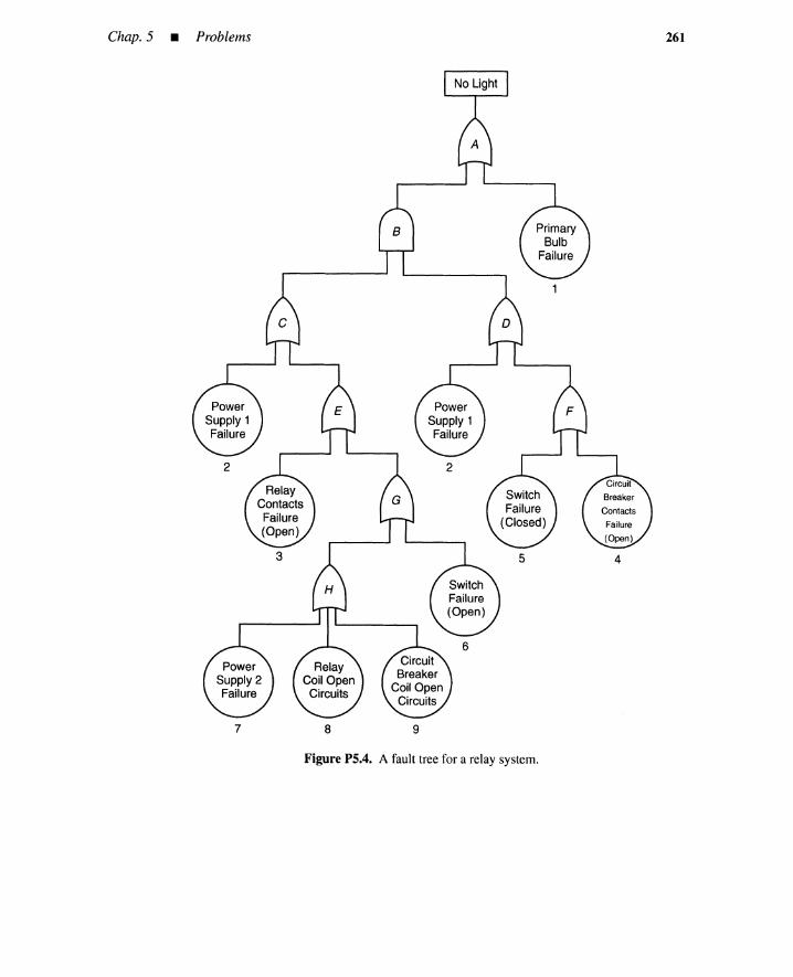
Chap. 5 • Problems
7 8 9
5 4
261
Figure P5.4. A fault tree for a relay system.
6uantification of BasicEvents
6.1 INTRODUCTION
All systems eventually fail; nothing is perfectly reliable, nothing endures forever. A relia-bility engineer must assume that a system will fail and, therefore, concentrate on decreasingthe frequency of failure to an economically and socially acceptable level. That is a morerealistic and tenable approach than are political slogans such as "zero pollution," "no risk,"and "accident-free."
Probabilistic statements are not unfamiliar to the public. We have become accus-tomed, for example, to a weather forecaster predicting that "there is a twenty percent risk ofthundershowers?" Likewise, the likelihood that a person will be drenched if her umbrellamalfunctions can be expressed probabilistically. For instance, one might say that there isa 80% chance that a one-year-old umbrella will work as designed. This probability is, ofcourse, time dependent. The reliability of an umbrella would be expected to decrease withtime; a two-year-old umbrella is more likely to fail than a one-year-old umbrella.
Reliability is by no means the only performance criterion by which a device such as anumbrella can be characterized. If it malfunctions or breaks, it can be repaired. Because theumbrella cannot be used while it is being repaired, one might also measure its performancein terms of availability, that is, the fraction of time it is available for use and functioningproperly. Repairs cost money, so we also want to know the expected number of failuresduring any given time interval.
Intuitively, one feels that there are analytical relationships between descriptions suchas reliability, availability, and expected number of failures. In this chapter, these relation-ships are developed. An accurate description of component failures and failure modes
*A comedianonceaskedwhetherthis statementmeantthat if youstoppedten peoplein the streetandaskedthem if it would rain, two of them would say "yes."
263

264 Quantification ofBasic Events - Chap. 6
is central to the identificationof system failures, because these are caused by combinationsof component failures. If there are no system-dependent component failures, then thequantification of basic (component) failures is independent of a particular system, andgeneralizations can be made. Unfortunately that is not usually the case.
In thischapter, we firstquantify basiceventsrelated to systemcomponents with binarystates, that is, normal and failed states. By components, we mean elementary devices,equipment, subsystems, and so forth. Then this quantification is extended to componentshaving plural failure modes. Finally,quantitativeaspects of human errors and impacts fromthe environment are discussed.
We assume that the reader has some knowledge of statistics. Statistical conceptsgeneric to reliability are developed in this chapter and additional material can be found inAppendix A.I to this chapter. A useful glossary of definitions appears as Appendix A.6.
There are a seemingly endless number of sophisticated definitions and equations inthis chapter, and the reader may wonder whether this degree of detail and complexity isjustified or whether it is a purely academic indulgence.
The first version of this chapter, which was written in 1975,was considerably simplerand contained fewerdefinitions. When this material wasdistributed at the NATO AdvancedStudy Institute on Risk Analysis in 1978, it became clear during the ensuing discussion thatthe (historical) absence of very precise and commonly understood definitions for failureparameters had resulted in theories of limited validity and computer programs that purportto calculate identical parameters but don't. In rewriting this chapter, we tried to set thingsright, and to label all parameters so that their meanings are clear. Much existing confusioncenters around the lack of rigor in defining failure parameters as being conditional orunconditional. Clearly, the probability of a person's living the day after their 30th birthdayparty is not the same as the probability of a person's living for 30 years and 1 day. Thelatter probability is unconditional, while the former is conditional on the person's havingsurvived to age thirty,
As alluded to in the preface, the numerical precision in the example problems is notwarranted in light of the normally very imprecise experimental failure data. The numbersare carried for ease of parameter identification.
6.2 PROBABILISTIC PARAMETERS
Weassume that, at any given time, a component is either functioning normally or failed, andthat the component state changes as time evolves. Possible transitions of state are shownin Figure 6.1. A new component "jumps" into a normal state and is there for some time,then fails and experiences a transition to the failed state. The failed state continues foreverif the component is nonrepairable. A repairable component remains in the failed state fora period, then undergoes a transition to the normal state when the repair is completed. Itis assumed that the component changes its state instantaneously when the transition takesplace. It is further assumed that, at most, one transition occurs in a sufficiently small timeinterval and that the possibility of two or more transitions is negligible.
The transition to the normal state is called repair, whereas the transition to the failedstate is failure. We assume that repairs restore the component to a condition as good asnew, so we can regard the factory production of a component as a repair. The entire cyclethus consists of repetitions of the repair-to-failureand the failure-to-repair process. We firstdiscuss the repair-to-failureprocess, then failure-to-repairprocess, and finallythe combinedprocess.
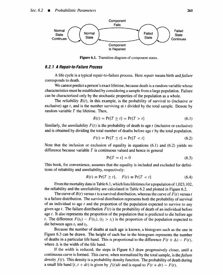
Sec. 6.2 • Probabilistic Parameters
ComponentFails
NormalState
Continues
ComponentIs Repaired
Figure 6.1. Transition diagram of component states.
6.2.1 ARepair-Io-Failure Process
FailedState
Continues
265
A life cycle is a typical repair-to-failure process. Here repair means birth andfailurecorresponds to death.
We cannot predict a person's exact lifetime, because death is a random variable whosecharacteristics must be established by considering a sample from a large population. Failurecan be characterized only by the stochastic properties of the population as a whole.
The reliability R(t), in this example, is the probability of survival to (inclusive orexclusive) age t, and is the number surviving at t divided by the total sample. Denote byrandom variable T the lifetime. Then,
R(t) == Pr{T 2: t} == Pr{T > t} (6.1)
Similarly, the unreliability F(t) is the probability of death to age t (inclusive or exclusive)and is obtained by dividing the total number of deaths before age t by the total population.
F(t) == Pr{T ::5 t} == Pr{T < t} (6.2)
Note that the inclusion or exclusion of equality in equations (6.1) and (6.2) yields nodifference because variable T is continuous valued and hence in general
Pr{T == t} == ° (6.3)
This book, for convenience, assumes that the equality is included and excluded for defini-tions of reliability and unreliability, respectively:
R(t) == Pr{T 2: t}, F(t) == Pr{T < t} (6.4)
From the mortality data in Table 6.1, which lists lifetimes for a population of 1,023, 102,the reliability and the unreliability are calculated in Table 6.2 and plotted in Figure 6.2.
The curve of R(t) versus t is a survival distribution, whereas the curve of F (z) versus t
is a failure distribution. The survival distribution represents both the probability of survivalof an individual to age t and the proportion of the population expected to survive to anygiven age t. The failure distribution F(t) is the probability of death of an individual beforeage t. It also represents the proportion of the population that is predicted to die before aget. The difference F(t2) - F(tl), (t2 > tl) is the proportion of the population expected todie between ages tl and tz-
Because the number of deaths at each age is known, a histogram such as the one inFigure 6.3 can be drawn. The height of each bar in the histogram represents the numberof deaths in a particular life band. This is proportional to the difference F(t + ~) - F(t),where t::. is the width of the life band.
If the width is reduced, the steps in Figure 6.3 draw progressively closer, until acontinuous curve is formed. This curve, when normalized by the total sample, is thefailuredensity f(t). This density is a probability density function. The probability of death duringa smalllife band [t, t + dt) is given by f(t)dt and is equal to F(t + dt) - F(t).

266 Quantification ofBasic Events - Chap. 6
TABLE 6.1. Mortality Data [I]
t L(t) t L(t) t L(t) t L(t)
0 1,023,102 15 962,270 50 810,900 85 78,221
1 1,000,000 20 951,483 55 754,191 90 21,577
2 994,230 25 939,197 60 677,771 95 3,011
3 990,114 30 924,609 65 577,822 99 125
4 986,767 35 906,554 70 454,548 100
5 983,817 40 883,342 75 315,982 0
10 971,804 45 852,554 80 181,765
t = age in yearsL(t) = number livingat age t
TABLE 6.2. Human Reliability
t L(t) R(t) = L(t)/N F(t) = 1 - R(t)
0 1,023,102 1.0000 0.0000
1 1,000,000 0.9774 0.0226
2 994,230 0.9718 0.0282
3 990,114 0.9678 0.0322
4 986,767 0.9645 0.0355
5 983,817 0.9616 0.0384
10 971,804 0.9499 0.0501
15 962,270 0.9405 0.0595
20 951,483 0.9300 0.0700
25 939,197 0.9180 0.0820
30 924,609 0.9037 0.0963
35 906,554 0.8861 0.1139
40 883,342 0.8634 0.1366
45 852,554 0.8333 0.1667
50 810,900 0.7926 0.2074
55 754,191 0.7372 0.2628
60 677,771 0.6625 0.3375
65 577,822 0.5648 0.4352
70 454,548 0.4443 0.5557
75 315,982 0.3088 0.6912
80 181,765 0.1777 0.8223
85 78,221 0.0765 0.9235
90 21,577 0.0211 0.9789
95 3,011 0.0029 0.9971
99 125 0.0001 0.9999
100 0 0.0000 1.0000
t = age in yearsL(t) = number livingat age t

Sec. 6.2 • Probabilistic Parameters 267
1.0
LL 0.9or;caQ) 0.8c-g 0.7ctS-~ 0.6
~ 0.5.~
~ 0.4....o~ 0.3
:0~ 0.2ctS.ce 0.1a..
Figure 6.2. Survival and failure distribu-tions.
o 10 20 30 40 50 60 70 80 90 100
Age in Years (t)
140
120
en"C 100c:ctSen::J0
or;
C 80en
or;caQ)
c 60'0Qi.0E::J 40Z
20
Figure 6.3. Histogram and smooth curve.o 20 40 60
Age in Years (t)80 100

268 Quantification ofBasic Events _ Chap. 6
The probability of death between ages tl and t: is the area under the curve obtainedby integrating the curve between the ages
F(t2) - F(tl) == 1" f(t)dt11
This identity indicates that the failure density j'(t) is
f(t) = dF(t)dt
(6.5)
(6.6)
and can be approximated by numerical differentiation when a smooth failure distribution isavailable, for instance, by a polynomial approximation of discrete values of F(t):
Letting
j' F(t + ~) - F(t)(t)::::-----
~(6.7)
(6.8)
(6.9)
N == total number of sample == 1,023,102
n (t) == number of deaths before age t
net + ~) == number of deaths before age t + ~
the quantity [net + ~) - n(t)]/N is the proportion of the population expected to die during[t, t + ~) and equals F(t + ~) - F(t). Thus
j' net + ~) - net)(t)::::----
/:1·N
The quantity [net + /:1) - net)] is equal to the height of the histogram in a life band[t, t + ~). Thus the numerical differentiation formula of equation (6.8) is equivalent to thenormalization of the histogram of Figure 6.3 divided by the total sample N and the bandwidth ~.
Calculated values for j'(t) are given in Table 6.3 and plotted in Figure 6.4. Column4 of Table 6.3 is based on a differentiation of curve F(t), and column 3 on a numericaldifferentiation (Le., the normalized histogram). Ideally, the values should be identical; inpractice, small sample size and numerical inaccuracies lead to differences in point val-ues.
Consider now a new population consisting of the individuals surviving at age t. Thefailure rate ret) is the probability of death per unit time at age t for the individual inthis population. Thus for sufficiently small ~, the quantity r(t) . ~ is estimated by thenumber of deaths during [t, t + ~) divided by the number of individuals surviving atage t:
number of deaths during [t, t + ~)ret) . ~ == -----------
number of survivals at age t
[net + ~) - net)]
L(t)
If we divide the numerator and the denominator by the total sample (N == 1,023,102),we have
r(t)tl = f(t)tlR(t)
(6.10)
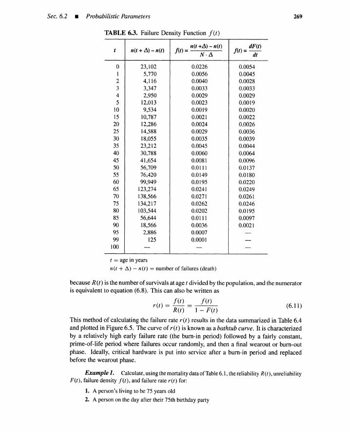
Sec. 6.2 • Probabilistic Parameters
TABLE 6.3. Failure Density Function I(t)
n(t + L\)- n(t) f(t) =n(t +L\) - n(t) ) dF(t)t
N·L\f(t =-
dt
0 23,102 0.0226 0.00541 5,770 0.0056 0.00452 4,116 0.0040 0.00283 3,347 0.0033 0.00334 2,950 0.0029 0.00295 12,013 0.0023 0.0019
10 9,534 0.0019 0.002015 10,787 0.0021 0.002220 12,286 0.0024 0.002625 14,588 0.0029 0.003630 18,055 0.0035 0.003935 23,212 0.0045 0.004440 30,788 0.0060 0.006445 41,654 0.0081 0.009650 56,709 0.0111 0.013755 76,420 0.0149 0.018060 99,949 0.0195 0.022065 123,274 0.0241 0.024970 138,566 0.0271 0.026175 134,217 0.0262 0.024680 103,544 0.0202 0.019585 56,644 0.0111 0.009790 18,566 0.0036 0.002195 2,886 0.0007 -99 125 0.0001 -
100 - - -
t = age in years
net + ~) - n(t) = number of failures (death)
269
because R (t) is the number of survivals at age t divided by the population, and the numeratoris equivalent to equation (6.8). This can also be written as
I(t) I(t)r(t) = R(t) = 1 - F(t) (6.11)
This method of calculating the failure rate r(t) results in the data summarized in Table 6.4and plotted in Figure 6.5. The curve of r(t) is known as a bathtub curve. It is characterizedby a relatively high early failure rate (the bum-in period) followed by a fairly constant,prime-of-life period where failures occur randomly, and then a final wearout or bum-outphase. Ideally, critical hardware is put into service after a bum-in period and replacedbefore the wearout phase.
Example 1. Calculate, using the mortality data of Table 6.1, the reliability R(t), unreliabilityF(t), failure density f'tt), and failure rate ret) for:
1. A person's living to be 75 years old
2. A person on the day after their 75th birthday party

270 Quantification ofBasic Events - Chap. 6
Figure 6.4. Failure density .1'(/).
1.4
1.2
1.0
-"---'to-.
~0.8
'(i)cQ)
cQ) 0.6....~'asLL
0.4
0.2
20 40 60 80
Age in Years (t)100
TABLE 6.4. Calculation of Failure Rate ret)
Age in Number of Failures Age in Number of FailuresYears (Death) r(t) =f(t)/R(t) Years (Death) r(t) =f(t)/R(t)
0 23,102 0.0226 40 30,788 0.00701 5770 0.0058 45 41,654 0.00982 4116 0.0041 50 56,709 0.01403 3347 0.0034 55 76,420 0.02034 2950 0.0030 60 99,949 0.02955 12,013 0.0024 65 123,274 0.0427
10 9534 0.0020 70 138,566 0.061015 10,787 0.0022 75 134,217 0.085020 12,286 0.0026 80 103,544 0.113925 14,588 0.0031 85 56,644 0.144830 18,055 0.0039 90 18,566 0.172135 23,212 0.0051 95 2886 0.2396
99 125 1.0000
Solution:
1. At age 75 (neglecting the additional day):
R(t) = 0.3088, F(t) = 0.6912 (Table 6.2)
.I'(t) = 0.02620 (Table 6.3)
r(l) = 0.08500 (Table 6.4)
(6.12)

Early Failures
Random Failures
Sec. 6.2 • Probabilistic Parameters
Figure 6.5. Failure rate ret) versus t.
0.2
-......~Q) 0.15caa:Q)~
.2
.(6 0.1u..
0.05
20
271
WearoutFailures
III
I I I I I I I I I I I I I60 80 100
t,Years
2. In effect, we start with a new population of N = 315,982 having the following character-istics, where t = 0 means 75 years.
n(t + Ll) - n(t)
L(t)/N 1- R(t) Table 6.3 N·Ll I(t)/R(t)
t L(t) R(t) F(t) n(t + Ll) - n(t) I(t) ret)
0 315,982 1.0000 0.0000 134,217 0.0850 0.08505 181,765 0.5750 0.4250 103,554 0.0655 0.1139
10 78,221 0.2480 0.7520 56,634 0.0358 0.144415 21,577 0.0683 0.9317 18,566 0.0118 0.172820 3,011 0.0095 0.9905 2,886 0.0023 0.242124 125 0.0004 0.9996 125 0.0004 1.000025 0 0.0000 1.0000 0 0.0000 -
By linear interpolation techniques, at 75 years and 1 day.
0.575 - 1R(t) = 1 + 5 x 365 = 0.9998
F(t) = 1 - R(t) = 0.0002
0.0655 - 0.0850j '(t ) = 0.085 + 6 = 0.0850, 5 x 3 5r(t) = 0.0850
Figure 6.6 shows the failure distribution for this population.
6.2.2 ARepair-Failure-Repair Process
(6.13)
•A repairable component experiences repetitions of the repair-to-failure and failure-
to-repair process. The characteristics of such components can be obtained by consideringthe component as a sample from a population of identical components undergoing similar
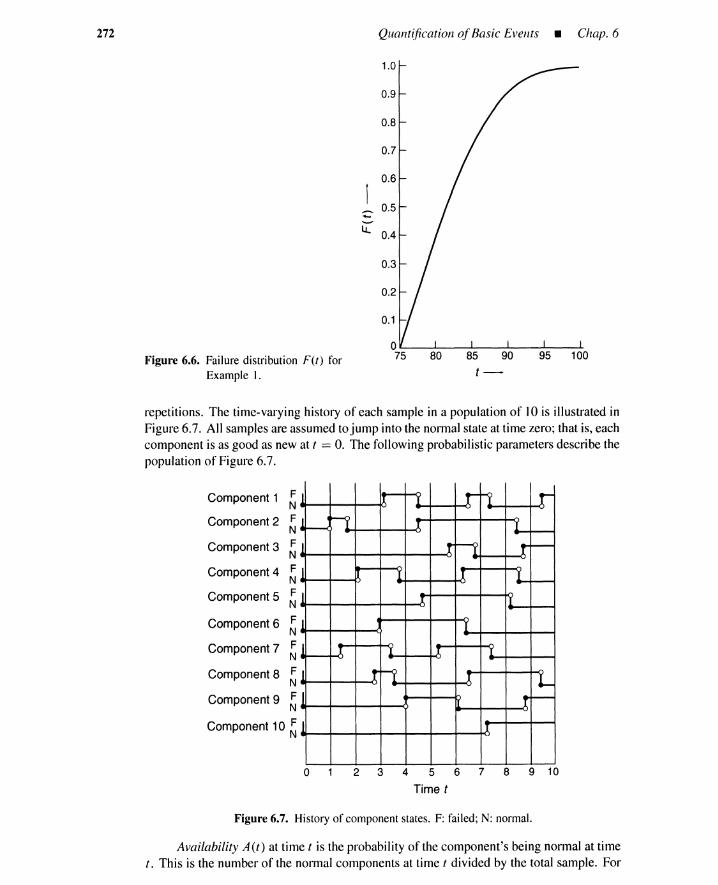
272 Quantification ofBasic Events - Chap. 6
1.0
0.9
0.8
0.7
0.6
- 0.5.....--LL 0.4
0.3
0.2
0.1
Figure 6.6. Failure distribution F(t) forExample I.
80 85 90
t-95 100
repetitions. The time-varying history of each sample in a population of lOis illustrated inFigure 6.7. All samples are assumed tojump into the normal state at time zero; that is, eachcomponent is as good as new at t == O. The following probabilistic parameters describe thepopulation of Figure 6.7.
Component 1 ~
Component 2 ~
Component 3 ~
Component 4 ~
Component 5 ~
Component 6 ~
Component 7 ~
Component 8 ~
Component 9 ~
Component 10 ~
1 I I r-~ r-J~H I I
1 tH r I---
-1 I I I L-I---1 I I
1 J I
j I I I I
1 t~ I 1-1 I t~
J I
o 2 3 4 5 6 7 8 9 10
Time t
Figure 6.7. Historyof componentstates. F: failed; N: normal.
Availability A(t) at time t is the probability of the component's being normal at timet. This is the number of the normal components at time t divided by the total sample. For

Sec. 6.2 • Probabilistic Parameters 273
our sample, we have A(5) == 6/10 == 0.6. Note that the normal components at time t havedifferent ages, and that these differ from t. For example, component 1 in Figure 6.7 has age0.5 at time 5, whereas component 4 has age 1.2.
Unavailability Q(t) is the probability that the component is in the failed state at timet and is equal to the number of the failed components at time t divided by the total sample.
Unconditionalfailure intensity w(t) is the probability that the component fails perunit time at time t. Figure 6.7 shows that components 3 and 7 fail during time period [5, 6),so w(5) is approximated by 2/10 == 0.2.
The quantity w(5) x 1 is equal to the expected number offailures W (5,6) during thetime interval [5,6). The expected number of failures W(O, 6) during [0,6) is evaluated by
W(O, 6) == w(O) x 1 + ... + w(5) x 1 (6.14)
The exact value of W (0, 6) is given by the integration
W(O, 6) =16
w(t)dt (6.15)
Unconditional repair intensity v(t) and expected number of repairs V (tl, t2) can bedefined similarly to w(t) and W(tl, t2), respectively. The costs due to failures and repairsduring [tl, t2) can be related to W(tl, t2) and V (tl, t2), respectively, if the production lossesfor failure and cost-to-repair are known.
There is yet another failure parameter to be obtained. Consider another population ofcomponents that are normal at time t. When t == 5, this population consists of components1,3,4,7,8, and 10. A conditional failure intensity A(t) is the proportion of the (normal)population expected to fail per unit time at time t. For example, A x 1 is estimated as2/6, because components 3 and 7 fail during [5,6). A conditional repair intensity /.L(t) isdefined similarly. Large values of A(t) mean that the component is about to fail, whereaslarge values .of /.L(t) state that the component will be repaired soon.
Example 2. Calculate values for R(t), F(t), j'(t), r(t), A(t), Q(t), w(t), W (0, t), and A(t)for the 10 components of Figure 6.7 at 5 hr and 9 hr.
Solution: We need times to failures (i.e., lifetimes) to calculate R(t), F(t), ,l(t), and r(t), becausethese are parameters in the repair-to-failure process.
Component Repair t Failure t TTF
1 0 3.1 3.11 4.5 6.6 2.11 7.4 9.5 2.12 0 1.05 1.052 1.7 4.5 2.83 0 5.8 5.83 6.8 8.8 2.04 0 2.1 2.14 3.8 6.4 2.65 0 4.8 4.86 0 3.0 3.07 0 1.4 1.47 3.5 5.4 1.98 0 2.85 2.858 3.65 6.7 3.059 0 4.1 4.19 6.2 8.95 2.75
10 0 7.35 7.35

274 Quantification ofBasic Events _ Chap. 6
The following mortality data is obtained from these times to failures.
t L(t) R(t) F(t) Il(t + L\) - Il(t) f(t) r(t) =f(t)/R(t)
0 18 1.0000 0.0000 0 0.0000 0.00001 18 1.0000 0.0000 3 0.1667 0.16672 15 0.8333 0.1667 10 0.5556 0.66673 7 0.3889 0.6111 3 0.1667 0.42864 4 0.2222 0.7778 2 0.1111 0.50005 2 0.1111 0.8889 1 0.0556 0.50056 I 0.0556 0.9444 0 0.0000 0.00007 I 0.0556 0.9444 1 0.0556 1.00008 0 0.0000 1.0000 0 0.0000 -9 0 0.0000 1.0000 0 0.0000 -
Thus at age 5,
R(5) = 0.1111,
and at age 9,
F(5) = 0.8889, .1'(5) = 0.0556, r(5) = 0.5005 (6.16)
R(9) = 0, F(9) = I, .1'(9) = 0, r(9): undefined (6.17)
Parameters A(t), Q(t), w(t), W(O, t), and A(t) are obtained from the combined repair-failure-repairprocess shown in Figure 6.7. At time 5,
and at time 9,
A(5) = 6/10 = 0.6, Q(5) = 0.4, w(5) = 0.2
W(O, 5) = [2 + 2 + 2 + 3] = 0.9, A(5) = 2/6 = 1/310
(6.18)
(6.19)
A(9) = 6/10 = 0.6, Q(9) = 0.4, w(9) == 0.1 (6.20)
W(O 9) == W(O 5) + [2+3+ 1 +2] == 1.7, , 10 ' A(5) == 1/6 (6.21)
•6.2.3 Paramelers ofRepair-la-Failure Process
Wereturn nowto the problem of characterizing the reliabilityparameters for repair-to-failure processes. These processes apply to nonrepairablecomponents and also to repairablecomponents if we restrict our attention to times to the first failures. We first restate someof the concepts introduced in Section 6.2.1, in a more formal manner, and then deduce newrelations.
Consider a process starting at a repair and ending in its first failure. Shift the timeaxis appropriately, and take t == 0 as the time at which the component is repaired, so thatthe component is then as good as new at time zero. The probabilistic definitions and theirnotations are summarized as follows:
R(t) == reliability at time t:
The probability that the component experiences no failure during thetime interval [0, t], given that the component was repaired at time zero.
The curve R(t) versus t is a survival distribution. The distribution is monotoni-cally decreasing, because the reliability gets smaller as time increases. A typical survivaldistribution is shown in Figure 6.2.
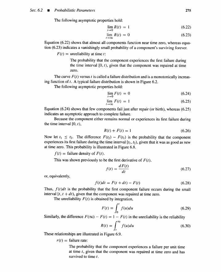
Sec. 6.2 • Probabilistic Parameters 275
The following asymptotic properties hold:
lim R(t) == 1t~O
lim R(t) == 0t~oo
(6.22)
(6.23)
Equation (6.22) shows that almost all components function near time zero, whereas equa-tion (6.23) indicates a vanishingly small probability of a component's surviving forever.
F(t) == unreliability at time t:
The probability that the component experiences the first failure duringthe time interval [0, t), given that the component was repaired at timezero.
(6.24)
(6.25)lim F(t) == 1t~oo
The curve F(t) versus t is called a failure distribution and is a monotonically increas-ing function of t. A typical failure distribution is shown in Figure 6.2.
The following asymptotic properties hold:
lim F(t) == 0t~O
Equation (6.24) shows that few components fail just after repair (or birth), whereas (6.25)indicates an asymptotic approach to complete failure.
Because the component either remains normal or experiences its first failure duringthe time interval [0, t),
R(t) + F(t) == 1 (6.26)
Now let t} :s tz- The difference F(t2) - F(tl) is the probability that the componentexperiences its first failure during the time interval [II, t2), given that it was as good as newat time zero. This probability is illustrated in Figure 6.8.
f(t) == failure density of F(t).
This was shown previously to be the first derivative of F(t).
J(t) = d F(t) (6.27)dt
or, equivalently,
f'(t)dt == F(t + dt) - F(t) (6.28)
Thus, f(t)dt is the probability that the first component failure occurs during the smallinterval [t, t + dt), given that the component was repaired at time zero.
The unreliability F(t) is obtained by integration,
F(t) = it j(u)du (6.29)
Similarly, the difference F(oo) - F(t) == 1 - F(t) in the unreliability is the reliability
R(t) =100
j(u)du (6.30)
These relationships are illustrated in Figure 6.9.
r(t) == failure rate:
The probability that the component experiences a failure per unit timeat time t, given that the component was repaired at time zero and hassurvived to time t.
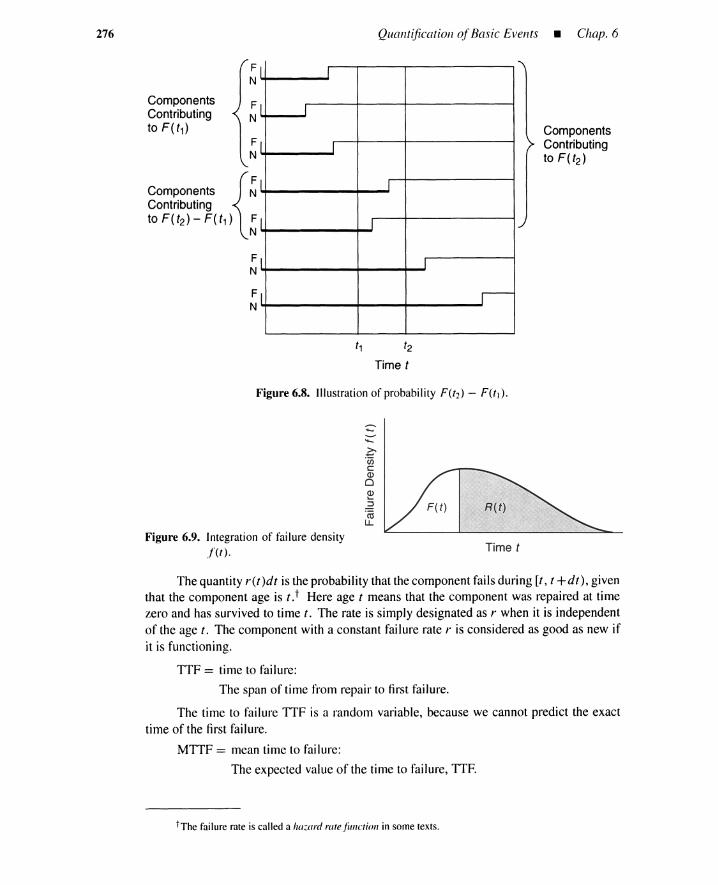
276 Quantification of Basic Events _ Chap. 6
{
FComponents NContributingtoF(t2)-F(t1l ~
ComponentsContributingto F(t1)
FN
FN
FN
FN
FN
I.,
I
I I
I I
I I
I I .J
I I
I r-
ComponentsContributingto F(t2)
Figure 6.8. Illustration of probability F(t2) - F(tt).
Figure 6.9. Integration of failure densitylet). Time t
The quantity r(t)dt is the probabilitythat thecomponent failsduring [t, t +dt), giventhat the component age is t. t Here age t means that the component was repaired at timezero and has survived to time t. The rate is simply designated as r when it is independentof the age t. The component with a constant failure rate r is considered as good as new ifit is functioning.
TTF = time to failure:
The span of time from repair to first failure.
The time to failure TTF is a random variable, because we cannot predict the exacttime of the first failure.
MTTF = mean time to failure:
The expected value of the time to failure, TIE
tThe failure rate is called a hazard ratefunction in some texts.
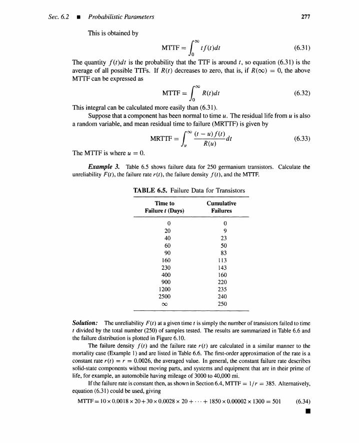
Sec. 6.2 • Probabilistic Parameters
This is obtained by
277
MTTF =100
tf(t)dt (6.31)
The quantity f(t)dt is the probability that the TTF is around t, so equation (6.31) is theaverage of all possible TTFs. If R(t) decreases to zero, that is, if R(oo) = 0, the aboveMTTF can be expressed as
MTTF =100
R(t)dt (6.32)
This integral can be calculated more easily than (6.31).Suppose that a component has been normal to time u. The residual life from u is also
a random variable, and mean residual time to failure (MRTfF) is given by
MRTIF = roo (t - u)f(t) dt (6.33)Ju R(u)
The MTTF is where u = o.Example 3. Table 6.5 shows failure data for 250 germanium transistors. Calculate the
unreliability F(t), the failure rate r(t), the failure density j'(t), and the MTIF.
TABLE 6.5. Failure Data for Transistors
Time toFailure t (Days)
o20406090
160230400900
12002500
00
CumulativeFailures
o9
235083
113143160220235240250
Solution: The unreliability F(t) at a given time t is simply the number of transistors failed to timet divided by the total number (250) of samples tested. The results are summarized in Table 6.6 andthe failure distribution is plotted in Figure 6.10.
The failure density j'(t) and the failure rate r(t) are calculated in a similar manner to themortality case (Example 1) and are listed in Table 6.6. The first-order approximation of the rate is aconstant rate r(t) = r = 0.0026, the averaged value. In general, the constant failure rate describessolid-state components without moving parts, and systems and equipment that are in their prime oflife, for example, an automobile having mileage of 3000 to 40,000 mi.
If the failure rate is constant then, as shown in Section 6.4, MTTF = 1/ r = 385. Alternatively,equation (6.31) could be used, giving
MTIF= 10 x 0.0018 x 20+30 x 0.0028 x 20 + ... + 1850 x 0.00002 x 1300 = 501 (6.34)
•
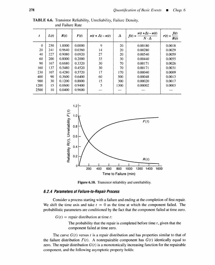
278 Quantification ofBasic Events - Chap. 6
TABLE 6.6. Transistor Reliability, Unreliability, Failure Density,and Failure Rate
t L(t) R(t) F(t) n(t + L\) - n(t) L\ f(t) =n(t +L\) - n(t) r(t) =f(t)
N·L\ R(t)
0 250 1.0000 0.0000 9 20 0.00180 0.001820 241 0.9640 0.0360 14 20 0.00280 0.002940 227 0.9080 0.0920 27 20 0.00540 0.005960 200 0.8000 0.2000 33 30 0.00440 0.005590 167 0.6680 0.3320 30 70 0.00171 0.0026
160 137 0.5480 0.4520 30 70 0.00171 0.0031230 107 0.4280 0.5720 17 170 0.00040 0.0009400 90 0.3600 0.6400 60 500 0.00048 0.0013900 30 0.1200 0.8800 15 300 0.00020 0.0017
1200 15 0.0600 0.9400 5 1300 0.00002 0.00032500 10 0.0400 0.9600 - - - -
1.2
-.....-lJ-. 1.0
~:0.~ 0.8Q)~
c:::::> 0.6-.....Cf
0.4~:.c.~ 0.2CDa:
200 400 600 800 1000 1200 1400 1600
Time to Failure (min)
Figure 6.10. Transistor reliability and unreliability.
6.2.4 Paramelers ofFailure-la-Repair Process
Consider a process starting with a failure and ending at the completion of first repair.We shift the time axis and take t == 0 as the time at which the component failed. Theprobabilistic parameters are conditioned by the fact that the component failed at time zero.
G(t) == repair distribution at time t:
The probability that the repair is completed before time t , given that thecomponent failed at time zero.
The curve G(t) versus t is a repair distribution and has properties similar to that ofthe failure distribution F(t). A nonrepairable component has G(t) identically equal tozero. The repair distribution G(t) is a monotonically increasing function for the repairablecomponent, and the following asymptotic property holds:
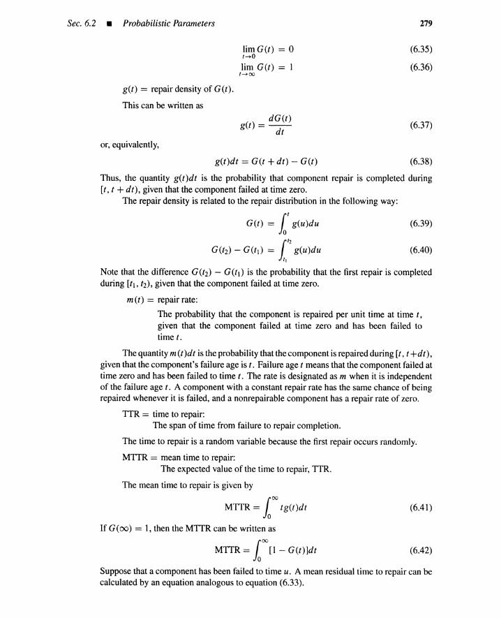
Sec. 6.2 • Probabilistic Parameters
lim G(t) = 01~O
lim G(t) = 11~oo
get) = repair density of G(t).
This can be written as
dG(t)get) =--
dt
or, equivalently,
g(t)dt = G(t + dt) - G(t)
279
(6.35)
(6.36)
(6.37)
(6.38)
(6.39)
(6.40)
(6.41)
(6.42)
Thus, the quantity get )dt is the probability that component repair is completed during[t, t + dt), given that the component failed at time zero.
The repair density is related to the repair distribution in the following way:
G(t) = 1t
g(u)du
112
G(t2) - G(tl) = g(u)du11
Note that the difference G(t2) - G(t}) is the probability that the first repair is completedduring [tl, ti), given that the component failed at time zero.
met) = repair rate:
The probability that the component is repaired per unit time at time t,given that the component failed at time zero and has been failed totime t.
The quantity m(t)dt is the probability that the component is repaired during [t , t +dt),given that the component's failure age is t. Failure age t means that the component failed attime zero and has been failed to time t. The rate is designated as m when it is independentof the failure age t. A component with a constant repair rate has the same chance of beingrepaired whenever it is failed, and a nonrepairable component has a repair rate of zero.
TTR = time to repair:The span of time from failure to repair completion.
The time to repair is a random variable because the first repair occurs randomly.
MTTR = mean time to repair:The expected value of the time to repair, TTR.
The mean time to repair is given by
MTTR =100
tg(t)dt
If G ((0) = 1, then the MTTR can be written as
MTIR = 100
[1 - G(t)]dt
Suppose that a component has been failed to time u. A mean residual time to repair can becalculated by an equation analogous to equation (6.33).
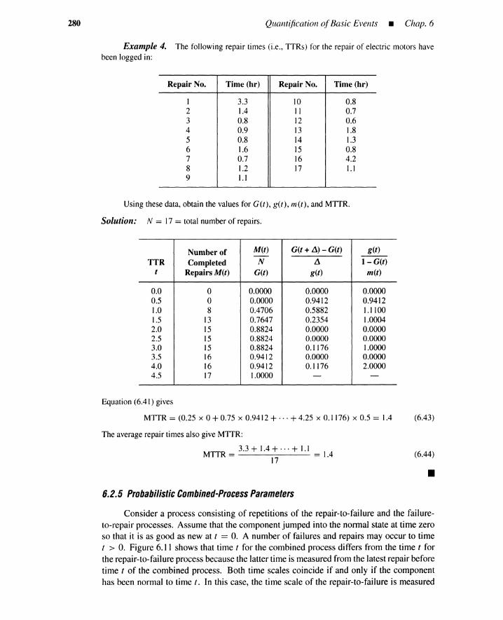
280 Quantification ofBasic Events _ Chap. 6
Example 4. The following repair times (i.e., TTRs) for the repair of electric motors havebeen logged in:
Repair No. Time (hr) Repair No. Time (hr)
1 3.3 10 0.82 1.4 11 0.73 0.8 12 0.64 0.9 13 1.85 0.8 14 1.36 1.6 15 0.87 0.7 16 4.28 1.2 17 1.19 1.1
Using these data, obtain the values for G(t), g(t), mtt ), and MITR.
Solution: N = 17 = total number of repairs.
Number of M(t) G(t + L\) - G(t) get)-
TTR Completed N L\ 1- G(t)t Repairs M(t) G(t) get) met)
0.0 0 0.0000 0.0000 0.00000.5 0 0.0000 0.9412 0.94121.0 8 0.4706 0.5882 1.11001.5 13 0.7647 0.2354 1.00042.0 15 0.8824 0.0000 0.00002.5 15 0.8824 0.0000 0.00003.0 15 0.8824 0.1176 1.00003.5 16 0.9412 0.0000 0.00004.0 16 0.9412 0.1176 2.00004.5 17 1.0000 - -
Equation (6.41) gives
MTTR = (0.25 x 0 + 0.75 x 0.9412 + ... + 4.25 x 0.1176) x 0.5 = 1.4 (6.43)
The average repair times also give MITR:
3.3 + 1.4 + ... + 1.1MITR = = 1.4
17
6.2.5 Probabilistic Combined-Process Parameters
(6.44)
•Consider a process consisting of repetitions of the repair-to-failure and the failure-
to-repair processes. Assume that the component jumped into the normal state at time zeroso that it is as good as new at t == O. A number of failures and repairs may occur to timet > O. Figure 6.11 shows that time t for the combined process differs from the time t forthe repair-to-failure process because the latter time is measured from the latest repair beforetime t of the combined process. Both time scales coincide if and only if the componenthas been normal to time t. In this case, the time scale of the repair-to-failure is measured

Sec. 6.2 • Probabilistic Parameters 281
from time zero of the combined process because the component is assumed to jump intothe normal state at time zero. Similarly, time t for the combined process differs from thetime t of the failure-to-repair process. The probabilistic concepts for the combined processare summarized as follows.
A (t) = availability at time t:
The probability that the component is normal at time t, given that it wasas good as new at time zero.
1.0
Figure 6.11. Schematic curves of avail-ability A(t).
o
Availability A(t)of Nonrepairable Component
Time t
Reliability generally differs from availability because the reliability requires the con-tinuation of the normal state over the whole interval [0, t]. A component contributes to theavailability A (t) but not to the reliability R (t) if the component failed before time t , is thenrepaired, and is normal at time t. Thus the availability A (t) is larger than or equal to thereliability R(t):
A(t) :::: R(t) (6.45)
The equality in equation (6.45) holds for a nonrepairable component because thecomponent is normal at time t if and only if it has been normal to time t. Thus
A(t) = R(t), for nonrepairable components (6.46)
The availability of a nonrepairable component decreases to zero as t becomes larger,whereas the availability ofthe repairable component converges to a nonzero positive number.Typical curves of A(t) are shown in Figure 6.11.
Q(t) = unavailability at time t:
The probability that the component is in the failed state at time t, giventhat it was as good as new at time zero.
Because a component is either in the normal state or in the failed state at time t, theunavailability Q(t) is obtained from the availability and vice versa:
A(t) + Q(t) = 1
From equations (6.26), (6.45), and (6.47), we have the inequality
Q(t) :::; F(t)
(6.47)
(6.48)
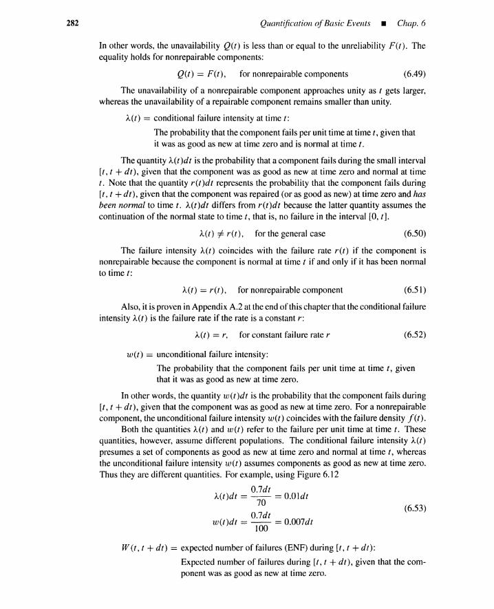
282 Quantification ofBasic Events - Chap. 6
In other words, the unavailability Q(t) is less than or equal to the unreliability F(t). Theequality holds for nonrepairablecomponents:
Q(t) == F(t), for nonrepairablecomponents (6.49)
The unavailability of a nonrepairable component approaches unity as t gets larger,whereas the unavailability of a repairable component remains smaller than unity.
A(t) == conditional failure intensity at time t:
The probability that the component fails per unit time at time t, given thatit was as good as new at time zero and is normal at time t.
The quantity A(t)dt is the probability that a component fails during the small interval[r, t + dt), given that the component was as good as new at time zero and normal at timet. Note that the quantity r(t)dt represents the probability that the component fails during[z, t +dt), given that the component was repaired (or as good as new) at time zero and hasbeen normal to time t. A(t)dt differs from r(t)dt because the latter quantity assumes thecontinuation of the normal state to time t, that is, no failure in the interval [0, t].
A(t) i= ret), for the general case (6.50)
The failure intensity A(t) coincides with the failure rate ret) if the component isnonrepairable because the component is normal at time t if and only if it has been normalto time t:
A(t) == ret), for nonrepairablecomponent (6.51 )
Also, it is provenin Appendix A.2 at the end of this chapter that the conditional failureintensity A(t) is the failure rate if the rate is a constant r:
A(t) == r, for constant failure rate r (6.52)
(6.53)
wet) == unconditional failure intensity:
The probability that the component fails per unit time at time t , giventhat it was as good as new at time zero.
In other words, the quantity w(t)dt is the probability that the component fails during[r , t + dt), given that the component was as good as new at time zero. For a nonrepairablecomponent, the unconditionalfailure intensity wet) coincides with the failure density J(t).
Both the quantities A(t) and wet) refer to the failure per unit time at time t. Thesequantities, however, assume different populations. The conditional failure intensity A(t)presumes a set of components as good as new at time zero and normal at time t, whereasthe unconditional failure intensity wet) assumes components as good as new at time zero.Thus they are different quantities. For example, using Figure 6.12
0.7dtA(t)dt == -- = O.Oldt
70
0.7dtw(t)dt == -- == 0.007dt
100
W (t, t + dt) == expected number of failures (ENF) during [z, t + dt):
Expected number of failures during [z, t + dt), given that the com-ponent was as good as new at time zero.

Sec. 6.2 • Probabilistic Parameters
Components Failingat Time t
Components Functioningat Time t
Figure 6.12. Conditional intensity A(t) and unconditional intensity w(t).
From the definition of the expected values, we have
00
W(t, t + dt) == L i . Pr{i failures during [t, t + dt)IC}i=l
283
(6.54)
where condition C means that the component was as good as new at time zero. At most,one failure occurs during [t, t + dt) and we obtain
or, equivalently,
W(t, t + dt) == Pr{one failure during [t, t + dt)IC}
W (t, t + dt) == w(t)dt
(6.55)
(6.56)
(6.57)
The expected number of failures during [tl , t2) is calculated from the unconditional failureintensity w(t) by integration.
W (tl' t2) == ENF over interval [tl, t2):
Expected number of failures during [tl, ti), given that the componentwas as good as new at time zero.
W (tl, tz) is the integration of W (t, t + dt) over the interval [tl, tz). Thus we have
112
W (tl, t2) == w(t)dt11
The W(O, t) of a nonrepairable component is equal to F(t) and approaches unity ast gets larger. The W (0, t) of a repairable component goes to infinity as t becomes infinite.Typical curves of W (0, t) are shown in Figure 6.13. The asymptotic behavior of Wandother parameters are summarized in Table 6.9.
j.,t(t) == conditional repair intensity at time t:
The probability that the component is repaired per unit time at time t,given that the component was as good as new at time zero and is failedat time t.
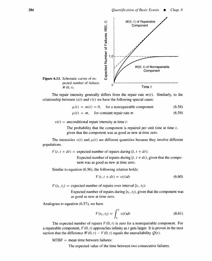
284 Quantification ofBasic Events _ Chap. 6
Figure 6.13. Schematic curves of ex-pected number of failuresW(O,t).
....--e-
ci~CI'JQ)~
~'(0u..'0~
Q).0 1.0E::JZ"CQ)
UQ)0-x
W
0
W(O, t) of RepairableComponent
W(O, t) of NonrepairableComponent
Time t
The repair intensity generally differs from the repair rate m(t). Similarly, to therelationship between A(I) and r(t) we have the following special cases:
Jl (I) == m(I) == 0, for a nonrepairable component
Jl(I) == m, for constant repair rate m
(6.58)
(6.59)
v(l) == unconditional repair intensity at time I:
The probability that the component is repaired per unit time at time I,
given that the component was as good as new at time zero.
The intensities v(l) and Jl(I) are different quantities because they involve differentpopulations.
V (t, I + dt) == expected number of repairs during [I, I + dtv:
Expected number of repairs during [t, I + dt), given that the compo-nent was as good as new at time zero.
Similar to equation (6.56), the following relation holds:
V (I, t + dt) == v(l)dl (6.60)
V (II, (2) == expected number of repairs over interval [II, (2):
Expected number of repairs during [II, (2), given that the component wasas good as new at time zero.
Analogous to equation (6.57), we have
1h
V (II, (2) == v(l)dl11
(6.61)
The expected number of repairs V (0, I) is zero for a nonrepairable component. Fora repairable component, V (0, I) approaches infinity as I gets larger. It is proven in the nextsection that the difference W (0, I) - V (0, I) equals the unavailability Q(I).
MTBF == mean time between failures:
The expected value of the time between two consecutive failures.
Sec. 6.3 • Fundamental Relations Among Probabilistic Parameters 285
The mean time between failures is equal to the sum of MTTF and MTTR:
MTBF = MTTF +MTTR (6.62)
MTBR == mean time between repairs:
The expected value of the time between two consecutive repairs.
The MTBR equals the sum of MTTF and MTTR and hence MTBF:
MTBR == MTBF == MTTF + MTTR (6.63)
•(6.64)
Example 5. For the data of Figure 6.7, calculate Jl(7), v(7), and V (0,5).
Solution: Six components are failed at t = 7. Among them, only two components are repairedduring unit interval [7, 8). Thus
Jl(7) = 2/6 = 1/3v(7) = 2/10 = 0.2
1 4
V(O,5) = 10 L {total number ofrepairs in [i, j + \)J;=0
1= W x (0+ 1 +0+3+ 1) =0.5
6.3 FUNDAMENTAL RELATIONS AMONG PROBABILISTICPARAMETERS
In the previous section, we defined various probabilistic parameters and their interrelation-ships. These relations and the characteristics of the probabilistic parameters are summarizedin Tables 6.7, 6.8, and 6.9. Table 6.7 refers to the repair-to-failure process, Table 6.8 tothe failure-to-repair process, and Table 6.9 to the combined process. These tables includesome new and important relations that are deduced in this section.
6.3. 1 Repair-la-Failure Paramelers
We shall derive the following relations:
(6.65)f(t)f(t)
r(t) - ---I - F(t) R(t)
F(t) = 1 - exp [-it r(U)dU] (6.66)
R(t) = exp [-it r(U)dU] (6.67)
f(t) = r(t) exp [-it r(U)dU] (6.68)
The first identity is used to obtain the failure rate r(t) when the unreliability F(t) andthe failure density j'(t) are given. The second through the fourth identities can be used tocalculate F(t), R(t), and f(t) when the failure rate r(t) is given.
The flow chart of Figure 6.14 shows general procedures for calculating the proba-bilistic parameters for the repair-to-failure process. The number adjacent to each arrow

286 Quantification ofBasic Events _ Chap. 6
TABLE 6.7. Relations Among Parameters for Repair-to-Failure Process
General Failure Rate ret)
1. R(t) + F(t) == I 7. R(t) = fX F(II)dll
2. R(O) == I, R(oo) == 0 8. MlTF == 100 t/(t)dt == 100 R(t)dto 0
3. F(O) == 0, F(oo) == I 9. r(t) == .l(t) .l(t)
I - F(t) R(t)
4.d F(t)
10. R(t) = exp [-1' r(lI)dll].I'(t) == dt
5. .l(t)dt == F(t + dt) - F(t) II. F(t) = I - exp [ -1' r(lI)dll]
6. F(t) = l' f iuvd u 12. I(t) = ret) exp [-1' r(U)dll]()
Constant Failure Rate ret)= A
13. R(t) == e- At
14. F(t) == I - e:"
15. lU) == Ae- A(
. I16. MTTF == -
A
TABLE 6.8. Relations Among Parameters for Failure-to-Repair Process
General Repair Rate mit)
1. G(O) == 0, G(oo) == I
dG(t)2. g(t) == dt
3. g(t)dt == G(t + tit) - G(t)
4. G(t) == l' g(lI)du()
5. G(t2) - G(tt) == 1" g(lI)dll(I
Ix IX6. MITR == tg(t)dt == [I - G(t)]dt() 0
g(t)7. m(t) == I _ G(t)
8. G(t) = I - exp [- l' m(U)dU]
9. g(t) = m(t)exp [ -1' m(U)du]
10. G(t) == I - e- ttt
I11. MITR == -
Il
Constant Repair Rate m(t) = J-L
12. g(t) == ue:"
13. Il == 0 (nonrepairable)

Sec. 6.3 • Fundamental Relations Among Probabilistic Parameters
TABLE 6.9. Relations Among Parameters for the Combined Process
287
Repairable
Fundamental Relations
Nonrepairable
1. A(t) + Q(t) = 1 A(t) + Q(t) == 12. A(t) > R(t) A (t) == R(t)
3. Q(t) < F(t) Q(t) = F(t)
4. wet) = f(t) +l' r« - u)v(u)du w(t) = .l(t)
5. v(t) = l' get - u)w(u)du v(t) = 0
6. W(t, t + dt) = w(t)dt W(t, t + dt) = w(t)dt
7. V(t, t + dt) = v(t)dt V(t,t+dt) == 0
1'28. W (t1, t2) = w(u)du W (t1, t2) == F(t2) - F(t1)tl
112
9. V (t1, t2) = v(u)du V (t1, t2) = 0tl
10. Q(t) = W(O, t) - V(O, t) Q(t) = W (0, t) = F(t)
11. A(t) = w(t) w(t)A(t)-
1 - Q(t) - 1- Q(t)
12. JL(t) = v(t)/Q(t) /1-(t) = 0
Stationary Values
13.14.
15.16.17.
MTBF = MTBR = MITF + MTTRo< A(oo) < 1, 0 < Q(oo) < 1
o < w(oo) < 00, 0 < v(oo) < 00
w(oo) = v(oo)
W(O, 00) = 00, V(O, 00) = 00
Remarks
MTBF = MTBR = 00
A(oo) = 0, Q(oo) = 1
w(oo) = 0, v(oo) = 0w(oo) = v(oo) = 0W(O, 00) = 1, V(O, 00) = 0
18.19.20.
w(t) f. A(t),
A(t) f. r(t),
w(t) f. f'tt),
v(t) f. /1-(t)
/1-(t) f. m(t)
v(t) f. g(t)
w(t) f. A(t),
A(t) = r(t),
w(t) = f'tt),
v(t) = /1-(t) = 0/1-(t) = m(t) = 0v(t) = g(t) = 0
corresponds to the relation identified in Table 6.7. Note that the first step in processingfailure data (such as the data in Tables 6.1 and 6.5) is to plot it as a histogram (Figure 6.3) orto fit it, by parameter estimation techniques, to a standard distribution (exponential, normal,etc.). Parameter-estimation techniques and failure distributions are discussed later in thischapter. The flow chart indicates that R(t), F(t), !(t), and r(t) can beobtained if anyoneof the parameters is known.
We now begin the derivation of identities (6.65) through (6.68) with a statement ofthe definition of a conditional probability [see equation (A.14), Appendix of Chapter 3].
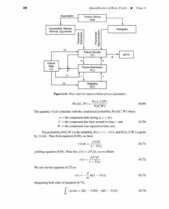
288 Quantification ofBasic Events - Chap. 6
Assumption
Exponential, Weibull,Normal, Log-normal
Time to FailureData
c-0m:;:;'E ~0,_c x>'000.Q..a.
«
FailureRater(t)
12
9
11
10 ReliabilityR(t)
Figure 6.14. Flow chart for repair-to-failureprocess parameters.
Pr{AIC W} = Pr{A, C1W}, Pr{CIW}
The quantity r(t)dt coincides with the conditional probability Pr{A IC, W} where
A == the component fails during [t, t + dt),
C == the component has been normal to time t, and
W == the component was repaired at time zero
(6.69)
(6.70)
(6.71)
The probability Pr{CI W} is the reliability R(t) == I - F(t), and Pr{A, CI W} is givenby j'(t)dt. Thus from equation (6.69), we have
j'(t)dtr(t)dt == ---
I - F(t)
yielding equation (6.65). Note that j'(t) == d Ffdt , so we obtain
dF/dtret) - ---
I - F(t)
We can rewrite equation (6.72) as
dret) == --In[1 - F(t)]
dt
Integrating both sides of equation (6.73),
l' r(u)du = In[1 - F(O)] - In[1 - F(t)]
(6.72)
(6.73)
(6.74)

Sec. 6.3 • Fundamental RelationsAmong Probabilistic Parameters 289
Substituting F(O) = 0 into equation (6.74)
1/ r(u)du = -In[1 - F(t)] (6.75)
(6.79)
(6.78)
(6.76)
(6.77)
yields equation (6.66). The remaining two identities are obtained from equations (6.26)and (6.27).
Consider, for example, failure density f(t).
f(t) = { t /2, 0 ~ t < 20, 2 ~ t
Failure distribution F(t), reliability R(t), and failure rate r(t) become
[
t 2/4, 0 < t < 2F(t) = -
1, 2 ~ t
R(t) = 1 _ F(t) == { 01,- (t2/4) , 0 ~ t < 2
2 ~ t
I t/2 0 < t < 2r(t) == f(t)/ R(t) == 1 - (t 2/ 4) , -
not defined, 2 ~ t
Mean time to failure MTTF is
MTTF =12
tf(t)dt =12
(t2/2)dt = [t
3/6]~ =4/3
This is also obtained from
(6.80)
MTTF = 12
R(t)dt = 12
I - (t2/4)dt = [t - (t 3/12)]~ = 4/3
6.3.2 Failure-to-Repair Parameters
(6.81)
Similar to the case of the repair-to-failure process, we obtain the following relationsfor the failure-to-repair process:
m(t) = g(t) (6.82)1 - G(t)
G(t) = I - exp [ -1/ m(U)du] (6.83)
g(t) = m(t) exp [ -1/ m(u)du ] (6.84)
The first identity is used to obtain the repair rate m(t) when the repair distributionG(t) and the repair density g(t) are given. The second and third identities calculate G(t)and g(t) when the repair rate m(u) is given.
The flow chart, Figure 6.15, shows the procedures for calculating the probabilisticparameters related to the failure-to-repair process. The number adjacent to each arrowcorresponds to Table 6.8. We can calculate G(t), g(t), and m(t) if anyone of them isknown.

290 Quantification ofBasic Events _ Chap. 6
Assumption
Exponential, Weibull,Normal, Log-normal
Time to RepairData
c-0co+::'E ~0._c x~o
00.a.. a.
«
RepairRatem(t)
9
7
8
6
Figure 6.15. Flow chart for failure-to-repair process parameters.
6.3.3 Combined-Process Parameters
General procedures for calculating combined-process probabilistic parameters areshown in Figure 6.16. The identification numbers in the flow chart are listed in Table 6.9.The chart includes some new and important relations that we now derive.
Densities f( t), g( t)
Unconditional Intensitiesw(t), v(t)
!8,9
Expected NumbersW(O, t), V(O, t)
!10
UnavailabilityO(t)
1 11, 12
Availability Conditional IntensitiesA(t) A(t), J.1( t)
Figure 6.16. Flow chart for the combined-process parameters.
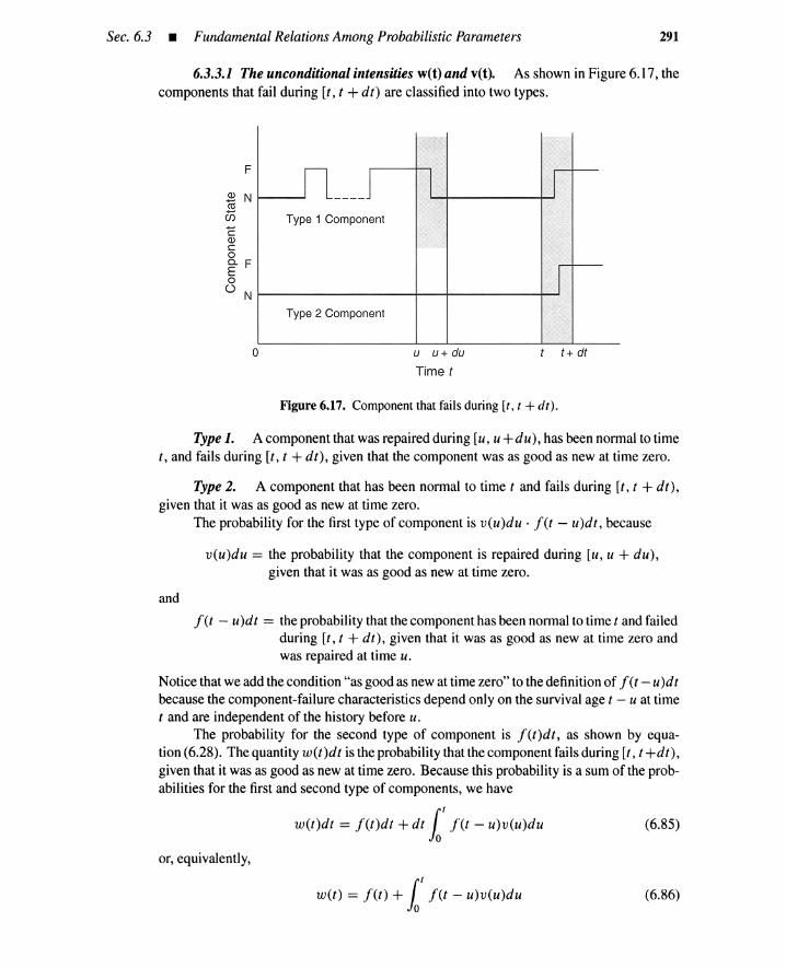
Sec. 6.3 • Fundamental Relations Among Probabilistic Parameters 291
6.3.3.1 The unconditional intensities w(t) and v(t). As shown in Figure 6.17,thecomponents that fail during [t, t + dt) are classified into two types.
F
OJ NiiiCi5COJCoEFoo N
___J I IType 1 Component
IType 2 Component
o u u+ du
Time t
Figure 6.17. Component that fails during [t, t + dt).
t + dt
(6.85)
Type 1. A component that was repaired during [u, u +du), has been normal to timet , and fails during [t, t + dt), given that the component was as good as new at time zero.
Type 2. A component that has been normal to time t and fails during [t, t + dt) ,given that it was as good as new at time zero.
The probability for the first type of component is v(u)du . f(t - u)dt, because
v(u)du = the probability that the component is repaired during [u, u + du),given that it was as good as new at time zero.
and
f(t - u)dt = the probability that the component has been normal to time t and failedduring [t, t + dt), given that it was as good as new at time zero andwas repaired at time u.
Notice that we add the condition "as good as new at time zero" to the definition of f(t -u)dtbecause the component-failure characteristics depend only on the survival age t - u at timet and are independent of the history before u.
The probability for the second type of component is f(t)dt, as shown by equa-tion (6.28) . The quantity w(t)dt is the probability that the component fails during [t, t +dt),given that it was as good as new at time zero . Because this probability is a sum of the prob-abilities for the first and second type of components, we have
w(t)dt = f(t)dt + dt 1/ f(t - u)v(u)du
or, equivalently,
w(t) = f(t) +1/f(t - u)v(u)du (6.86)
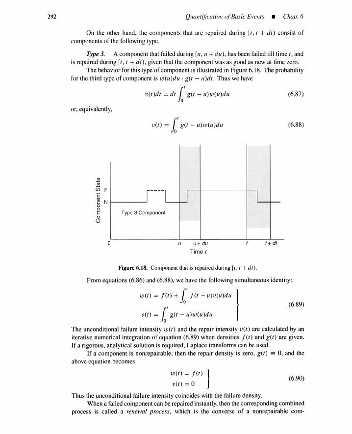
292 Quantification of Basic Events • Chap. 6
On the other hand, the components that are repaired during [r, t + dt) consist ofcomponents of the following type.
Type 3. A component that failed during [lI, 1I +dui, has been failed till time t, andis repaired during [t , t + dt], given that the component was as good as new at time zero.
The behaviorfor this type of component is illustratedin Figure6.18. The probabilityfor the third type of component is w(u)dll . get - uidt . Thus we have
v(t)dt = dt l' g(t - lI)w(lI)dll (6.87)
or, equivalently,
v(t) = l' g(t - lI)w(u)dll (6.88)
Q)
iiiCi5 F'E~ Noc.Eoo
----1 I IType 3 Component
o u u « du
Time tt+ dt
Figure6.18. Component that is repaired during [t, t + dt) .
From equations (6.86) and (6.88) , we have the following simultaneous identity:
w(t) = f(t) +l' f(t - lI)V(lI)dll 1(6.89)
v(t) = l' g(t - lI)w(lI)dll
The unconditional failure intensity w(t) and the repair intensity v(t) are calculated by aniterative numerical integration of equation (6.89) when densities f(t) and get) are given.If a rigorous, analytical solution is required, Laplace transformscan be used.
If a component is nonrepairable, then the repair density is zero, g(t) == 0, and theabove equation becomes
w(t) = f(t) I (6.90)vet) = 0
Thus the unconditional failure intensitycoincides with the failure density.Whena failedcomponentcan be repaired instantly, then the correspondingcombined
process is called a renewal process, which is the converse of a nonrepairable com-

Sec. 6.3 • Fundamental Relations Among ProbabilisticParameters 293
bined process. For the instant repair, the repair density becomes a delta function,g(t - u) = 8(t - u). Thus equation (6.89) becomes a so-called renewal equation, andthe expected number of renewals W (0, t) = V (0, t) can be calculated accordingly.
wet) = I(t) +11
I(t - u)w(u)du 1 (6.91)
v(t) = w(t)
6.3.3.2 Relations for calculating unavailability Q(t). Let x(t) be an indicatorvariable defined by
x(t) = 1,
x(t) = 0,
if the component is in a failed state, and
if the component is in a normal state
(6.92)
(6.93)
Represent by XO,l (t) and Xl,O(t) the numbers of failures and repairs to time t, respectively.Then we have
x(t) = XO,I (r) - XI,O(t) (6.94)
For example, if the component has experienced three failures and two repairs to time t , thecomponent state x (t) at time t is given by
x(t) = 3 - 2 = 1
As shown in Appendix A.3 of this chapter, we have
Q(t) = W(O, t) - V(O, t)
(6.95)
(6.96)
In other words, the unavailability Q(t) is given by the difference between the expectednumber of failures W (0, t) and repairs V (0, t) to time t. The expected numbers are obtainedfrom the unconditional failure intensity w(u) and the repair intensity v(u), according toequations (6.57) and (6.61). We can rewrite equation (6.96) as
Q(t) =11
[w(u) - v(u)]du (6.97)
6.3.3.3 Calculating the conditionalfailure intensity A(t). The simultaneous oc-currence of events A and C is equivalent to the occurrence of event C followed by event A[see equation (A.14), Appendix of Chapter 3]:
Pr{A, CIW} = Pr{CIW}P{AIC, W} (6.98)
(6.99)
Substitute the following events into equation (6.98):
C = the component is normal at time t,A = the component fails during [t, t + dt),W = the component was as good as new at time zero
At most, one failure occurs during a small interval, and the event A implies eventC. Thus the simultaneous occurrence of A and C reduces to the occurrence of A, andequation (6.98) can be written as
Pr{AIW} = Pr{CIW}P{AIC, W} (6.100)
According to the definition of availability A(t), conditional failure intensity )..,(t), andunconditional failure intensity w(t), we have
Pr{AIW} = w(t)dt (6.101)

294 Quantification ofBasic Events _ Chap. 6
Thus from equation (6.100),
or, equivalently,
and
Pr{A IC, W} == A(t)dt
Pr{C IW} == A(t )
wet) == A(t)A(t)
wet) == A(t)[1 - Q(t)]
(6.102)
(6.103)
(6.104)
(6.105)
A(t) = w(t) (6.106)1 - Q(t)
Identity (6.106) is used to calculate the conditional failure intensity A(t) when theunconditional failure intensity wet) and the unavailability Q(t) are given. Parameters wet)
and Q(t) can be obtained by equations (6.89) and (6.97), respectively.In the case of a constant failure rate, the conditional failure intensity coincides with
the failure rate r as shown by equation (6.52). Thus A(t) is known and equation (6.105) isused to obtain wet) from A(t) == rand Qtt),
6.3.3.4 Calculating fl{t). As in the case of A(t), we have the following identitiesfor the conditional repair intensity Jl(t):
vet)f1-(t) = Q(t) (6.107)
v(t) == Jl(t) Q(t) (6.108)
Parameter Jl(t) can be calculated using equation (6.107) when the unconditionalrepair intensity vet) and the unavailability Q(t) are known. Parameters vet) and Q(t) canbe obtained by equations (6.89) and (6.97), respectively.
When the component hasa constant repair rate m (t) == m, the conditional repair inten-sity is m and is known. In this case, equation (6.108) is used to calculate the unconditionalrepair intensity vet), given Jl(t) == m and Qtt),
If the component has a time-varying failure rate r(t), the conditional failure intensityA(t) does not coincide with ret). Similarly, a time-varying repair rate met) is not equal tothe conditional repair intensity Jl(t). Thus in general,
wet) i= r(t)[1 - Q(t)]
vet) i= n1(t)Q(t)
(6.109)
(6.110)
Example 6. Use the results of Examples 2 and 5 to confirm, in Table 6.9, relations (2), (3),(4), (5), (10), (11), and (12). Obtain the ITFs, TTRs, TBFs and TBRs for component 1.
Solution:
1. Inequality (2): From Example 2,
A(5) = 0.6 > R(5) = 0.1111
2. Inequality (3):
Q(5) = 0.4 < F(5) = 0.8889 (Example 2)
3. Equality (4): Weshall show that
w(5) = .1'(5) +15
f(5 - u)v(u)du()
(6.111)
(6.112)
(6.113)

Sec. 6.3 • Fundamental Relations Among Probabilistic Parameters
From Example 2,
w(5) = 0.2
295
(6.114)
The probability f'(5) x 1 refers to the component that has been normal to time 5 and failedduring [5,6), given that it was as good as new at time zero. Component 3 is identified, and we have
1./(5) = 10 (6.115)
The integral on the right-hand side of (6.113) refers to the components shown below.
Repaired Normal Failed Components
[0, 1) [1,5) [5,6) None[1, 2) [2,5) [5,6) None[2,3) [3,5) [5,6) None[3,4) [4,5) [5,6) Component 7[4,5) [5,6) None
Therefore,
is f(5 - u)v(u)du = 1/10
Equation (4) is confirmedbecause
1 10.2= - +-
10 10
4. Equality (5): We shall show that
v(7) = i7
g(5 - u)w(u)du
From Example 5,
v(7) = 0.2
The integral on the right-hand side refers to the components listed below.
Fails Failed Repaired Components
[0, 1) [1,7) [7,8) None[1,2) [2,7) [7,8) None[2,3) [3,7) [7,8) None[3,4) [4,7) [7,8) None[4,5) [5,7) [7,8) None[5,6) [6,7) [7,8) Component 7[6,7) [7,8) Component 1
Thus the integral is 2/10 = 0.2, and we confirm the equality.
5. Equality (10): We shall show that
Q(5) = W(O, 5) - V(O, 5)
(6.116)
(6.117)
(6.118)
(6.119)
(6.120)
From Example 2,
From Example 5,
Q(5) = 0.4, W(O, 5) = 0.9 (6.121)
V(O, 5) = 0.5 (6.122)

296 Quantification ofBasic Events - Chap. 6
Thus
0.4 = 0.9 - 0.5 (6.123)
Thus
and
6. Equality (11): From Example 2,
Q(S) = 0.4, w(S) = 0.2,
1 0.2
3 1 -0.4
w(S)A(S) = -1--Q-(-S)
A(5) = 1/3 (6.124)
(6.125)
(6.126)
is confirmed.
7. Equality (12): We shall show that
v(7)Jl(7) = Q(7)
From Example 5,
(6.127)
From Figure 6.7,
Jl(7) = 1/3, v(7) = 0.2 (6.128)
This is now confirmed, because
Q(7) = 6/10 = 0.6 (6.129)
1 0.2
3 0.6
8. TTFs, TTRs, TBFs, and TBRs are shown in Figure 6.19.
(6.130)
•
F
N
ITBR1 TBR2
4.5 2.9 - ~
TTF1 TTR1I-
TTF2I-
3.1 1.4 - 2.1 TTR20.8 TTF3
I+-2.1
10-
~- ~
3:1\ / \ V
4.5 6.6 7.4 9.5"
TBF1 TBF2f--
r- 3.5 2.9-r---
I Io 2 3 456
Time t7 8 9 10
Figure 6.19. Time history of component 1.
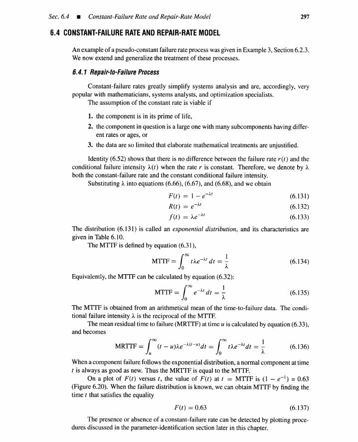
Sec. 6.4 • Constant-Failure Rate and Repair-Rate Model
6.4 CONSTANT-FAILURE RATE AND REPAIR-RATE MODEL
297
(6.131)
(6.132)
(6.133)
(6.135)
(6.134)
(6.136)
An exampleof a pseudo-constantfailure rate process wasgiven in Example 3, Section6.2.3.We now extend and generalize the treatment of these processes.
6.4.1 Repair-la-Failure Process
Constant-failure rates greatly simplify systems analysis and are, accordingly, verypopular with mathematicians, systems analysts, and optimization specialists.
The assumption of the constant rate is viable if
1. the component is in its prime of life,
2. the component in question is a large one with many subcomponentshavingdiffer-ent rates or ages, or
3. the data are so limited that elaborate mathematical treatments are unjustified.
Identity (6.52) shows that there is no difference between the failure rate r(t) and theconditional failure intensity A(t) when the rate r is constant. Therefore, we denote by Aboth the constant-failure rate and the constant conditional failure intensity.
Substituting Ainto equations (6.66), (6.67), and (6.68), and we obtain
F(t) == 1 - e-Af
R(t) == e-Af
j·(t) == Ae-Af
The distribution (6.131) is called an exponential distribution, and its characteristics aregiven in Table 6.10.
The MTTF is defined by equation (6.31),
100 1MTTF == o.e:" dt == -
o AEquivalently, the MTTF can be calculated by equation (6.32):
100 1MTTF == e-Af dt == -
o AThe MTTF is obtained from an arithmetical mean of the time-to-failure data. The condi-tional failure intensity Ais the reciprocal of the MTTF.
The mean residual time to failure (MRTTF)at time u is calculated by equation (6.33),and becomes
100 100 1MRTTF == (t - u)Ae-A(t-u)dt == tAe-Afdt == -u 0 A
When a component failure follows the exponentialdistribution,a normal component at timet is always as good as new. Thus the MRTTF is equal to the MTTF.
On a plot of F(t) versus t, the value of F(t) at t == MTTF is (1 - e- I ) = 0.63(Figure 6.20). When the failure distribution is known, we can obtain MTTF by finding thetime t that satisfies the equality
F(t) == 0.63 (6.137)
The presence or absence of a constant-failure rate can be detected by plotting proce-dures discussed in the parameter-identification section later in this chapter.
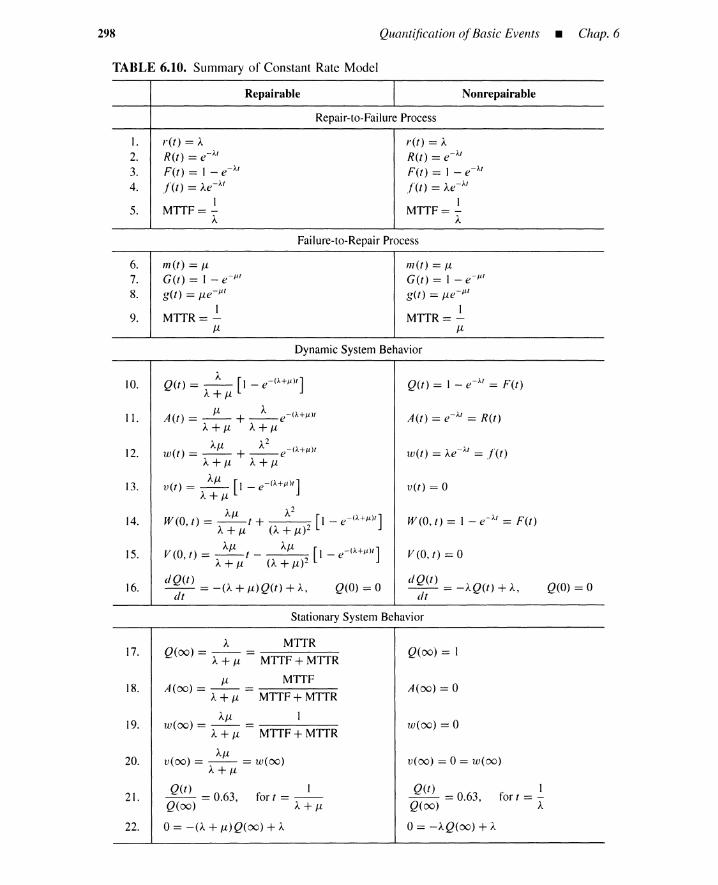
298
TABLE 6.10. Summary of Constant Rate Model
Repairable
QuantificationofBasic Events _ Chap. 6
Nonrepairable
I. r(t) = A2. R(t) = e- At
3. F(t) = 1 - e- A1
4. .l(t) = xe:"1
5. MTfF= -A
6. In(t) = J-l7. G(t) = 1 - «:"8. g(t) = ue:"
19. MTfR=-
J-l
Repair-to-Failure Process
r(t) = AR(t) = e- A1
F(t) = 1 - e- At
.l(t) = ie:"1
MTfF= -A
Failure-to-Repair Process
111(t) = J-lG(t) = 1 - «r'g(t) = ue:"
1MTTR= -
J-l
DynamicSystem Behavior
AQtt) = 1- e-
At = F(t)10. Q(t) = -- [1 - e-(A+/l)l]
A+J-l
II. A(t) = _11-_ + _A_ e- (A+ /l )l A(t) = e-At = R(t)A+J-l A+J-l
A A2
12. w(t) = _J-l_ + __ e-(A+/l)l w(t) = Ae- A1 = .l(t)A+J-l A+J-l
13. v(t) =~ [I - e-o,+;t)t] v(t) = 0A+J-l
A A2
14. W(O, t) = _11-_ t + . [I - e-(A+/1)l] W (0, t) = 1 - e - Al = F (t )A+ J-l (A+ J-l)2
15. V(O t) = ~t _ AJ1, [I - e-(A+IL)l] V (0, t) = 0, A+J1, (A+J1,)2
16. dQ(t) = -(A + J1,)Q(t) + A, Q(O) = 0 dQ(t) = -AQ(t) + A, Q(O) = 0dt dt
StationarySystem Behavior
A MTfR17. Q(oo) = A+ J1, = MTTF + MTTR Q(oo) = I
J1, MTTF18. A(oo) = A+ 11- = MTTF + MTTR A(oo) = 0
AJ-l 119.
1V(00) = A+ J-l = MTTF + MTfR w(oo) = 0
20.AJ1,
v(oo) = 0 = w(oo)v(oo) = -- = w(oo)A+J1,
Q(t) = 0.63 1 Q(t) = 0.63 121. fort =-- for t = -
Q(oo) , A+11- Q(oo) , A
22. o= -(A + J1,)Q(oo) + A o= -AQ(oo) + A
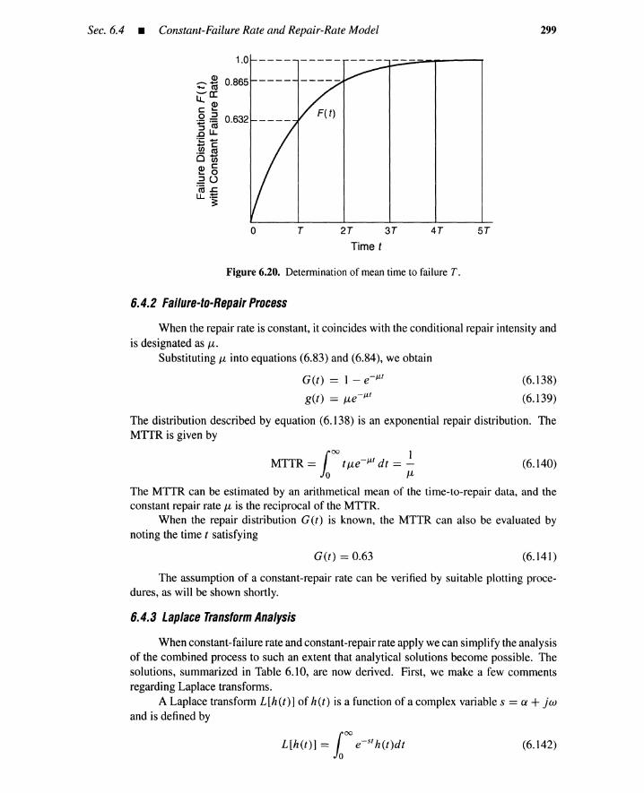
Sec. 6.4 • Constant-Failure Rate and Repair-RateModel
1.0
299
0.865
0.632 ----
o T 2T 3T
Time t
4T 5T
(6.138)
(6.139)
(6.140)
Figure 6.20. Determination of mean time to failure T.
6.4.2 Failure-la-Repair Process
When the repair rate is constant, it coincides with the conditional repair intensity andis designated as u:
Substituting Jvt into equations (6.83) and (6.84), we obtain
G(t) == 1 - e-/-Lf
get) == Jvte-J-if
The distribution described by equation (6.138) is an exponential repair distribution. TheMTfR is given by
100 1MTTR == tJvte-/-Lf dt == -
o Jvt
The MTTR can be estimated by an arithmetical mean of the time-to-repair data, and theconstant repair rate JL is the reciprocal of the MTfR.
When the repair distribution G(t) is known, the MTTR can also be evaluated bynoting the time t satisfying
G(t) == 0.63 (6.141)
The assumption of a constant-repair rate can be verified by suitable plotting proce-dures, as will be shown shortly.
6.4.3 Laplace Transform Analysis
When constant-failure rate and constant-repair rate apply we can simplify the analysisof the combined process to such an extent that analytical solutions become possible. Thesolutions, summarized in Table 6.10, are now derived. First, we make a few commentsregarding Laplace transforms.
A Laplace transform L[h(t)] of h(t) is a function of a complex variable s == ex + jtoand is defined by
L[h(t)) = 100
e-st h(t)dt (6.142)

300 Quantification ofBasic Events _ Chap. 6
For example, the transformation of e-a l is given by
100 1L[e-at ] == e-ste-atdt == --
o s+a(6.143)
(6.144)
(6.145)
An inverse Laplace transform L -I [R(s)] is a function of t having the Laplace trans-form R(s). Thus the inverse transformation of 1/(s + a) is «<.
L-I [s~a] =e-at
A significant characteristic of the Laplace transform is the following identity:
L [it hl(t -1l)h2(1l)dll] = L[h)(t)]· L[h2(t)]
In other words, the transformation of the convolution can be represented by the product ofthe two Laplace transforms L[hI(t)] and L[h2(t)]. The convolution integral is treated asan algebraic product in the Laplace-transformed domain.
Now we take the Laplace transform of equation (6.89):
L [w (t )] == L [j'(t )] + L [j' (t )] . L [v(t ) ] IL[v(t)] == L[g(t)] . L[w(t)]
The constant-failure rate A and the repair rate u. give
AL[j'(t)] == L[Ae-At
] == A . L[e-A/] == --
S+AJl
L[g(t)] == --s + Ji'
Thus equation (6.146) becomes
(6.146)
(6.147)
(6.148)
(6.149)
A AL[w(t)] == -- + --L[v(t)]
S+A S+A
L[v(t)] == _Jl-L[w(t)]s+Jl
Equation (6.149) is a simultaneous algebraic equation for L[w(t)] and L[v(t)] andcan be solved:
AJl ( 1) A2
( 1 )L[w(t)] == -- - +--A+Jl S A+Jl S+A+Jl
AJl ( 1) AJl ( 1 )L[v(t)] == -- - ---A+Jl S A+Jl S+A+Jl
Taking the inverse Laplace transform of equations (6.150) and (6.151) we have:
AJl ( 1) A2
( 1 )w(t) == --L- 1- + --L- 1
A+Jl S A+Jl S+A+Jl
All ( 1) All ( 1 )vet) == _I'-"'_L -I _ _ _I'-"'_L- I
A+Jl S A+Jl S+A+Jl
(6.150)
(6.151)
(6.152)
(6.153)
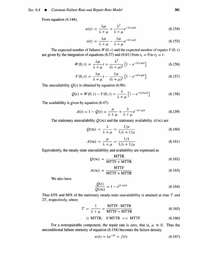
Sec. 6.4 • Constant-Failure Rate and Repair-RateModel
From equation (6.144),
301
(6.154)
(6.164)
AJ-t A2W(t) == -- + __ e-(A+t.t)1
A+J-t A+J-t
V(t) =~ - ~e-(A+Jl)1 (6.155)A+J-t A+J-t
The expected number of failures W (0, t) and the expected number of repairs V (0, t)
are given by the integration of equations (6.57) and (6.61) from tl == °to t: == t:
AJ-t A2
W(O, t) == --t + [1 - e-(A+t.t)I] (6.156)A+ J-t (A + J-t)2
V(O, t) = ~t - AIL [I - e-(A+Jl)I] (6.157)A+ J-t (A + J-t)2
The unavailability Q(t) is obtained by equation (6.96):
AQ(t) == W(O, t) - V(O, t) == -- [1 - e-(A+t.t)I] (6.158)
A+J-t
The availability is given by equation (6.47):
A(t) == 1 - Q(t) == _J-t_ + _A_ e - (A+ t.t)1 (6.159)A+J-t A+J-t
The stationary unavailability Q((0) and the stationary availability A (00) are
A I/J-tQ(oo) = A+ IL = IIA + IIIL (6.160)
J-t l/AA(oo) = A+ IL = IIA + 1IlL (6.161)
Equivalently, the steady-state unavailability and availability are expressed as
MTTRQ(oo) == MTTF + MTTR (6.162)
MTTFA(oo) - MTTF +MTTR (6.163)
We also have
Q(t) == 1 _ e(A+t.t)l
Q(oo)
Thus 63% and 86% of the stationary steady-state unavailability is attained at time T and2T, respectively, where
MTTF·MTTRT == -- == -----
A+ J-t MTTF + MTTR
~ MTTR, if MTTR < < MTTF
(6.165)
(6.166)
For a nonrepairable component, the repair rate is zero, that is, J-t == 0. Thus theunconditional failure intensity of equation (6.154) becomes the failure density.
w(t) == Ae-Af == j'(t) (6.167)
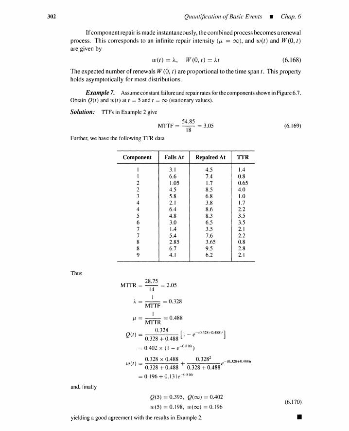
302 QuantificationofBasic Events - Chap. 6
Ifcomponentrepair is made instantaneously, thecombinedprocessbecomesa renewalprocess. This corresponds to an infinite repair intensity (J.l == (0), and w(t) and W(O,t)are given by
w(t) == A, W (0, t) == At (6.168)
The expected number of renewals W (0, t) are proportional to the time span t. This propertyholds asymptotically for most distributions.
Example 7. Assumeconstant failureandrepair ratesfor thecomponentsshowninFigure6.7.Obtain Q(t) and w(t) at t = 5 and t = 00 (stationary values).
Solution: TTFs in Example 2 give
54.85MTTF = -- = 3.05
18
Further, we have the followingTTR data
Component Fails At Repaired At TTR
1 3.1 4.5 1.4I 6.6 7.4 0.82 1.05 1.7 0.652 4.5 8.5 4.03 5.8 6.8 1.04 2.1 3.8 1.74 6.4 8.6 2.25 4.8 8.3 3.56 3.0 6.5 3.57 1.4 3.5 2.17 5.4 7.6 2.28 2.85 3.65 0.88 6.7 9.5 2.89 4.1 6.2 2.1
Thus28.75
MTfR = -- = 2.0514
1A = -- =0.328
MTTF1
J1 = MTTR = 0.488
0.328Q(t) = [1 - e-<O.J2S+0AS8)f]
0.328 + 0.488
= 0.402 x (I - e-O.816f)
w t _ 0.328 x 0.488 0.3282e-<O.328+0A88)f
( ) - 0.328 + 0.488 + 0.328 + 0.488
= 0.196 + 0.13Ie-o.816f
and,finally
Q(5) = 0.395, Q(oo) = 0.402
w(5) = 0.198, w(oo) = 0.196
yielding a good agreement with the results in Example 2.
(6.169)
(6.170)
•
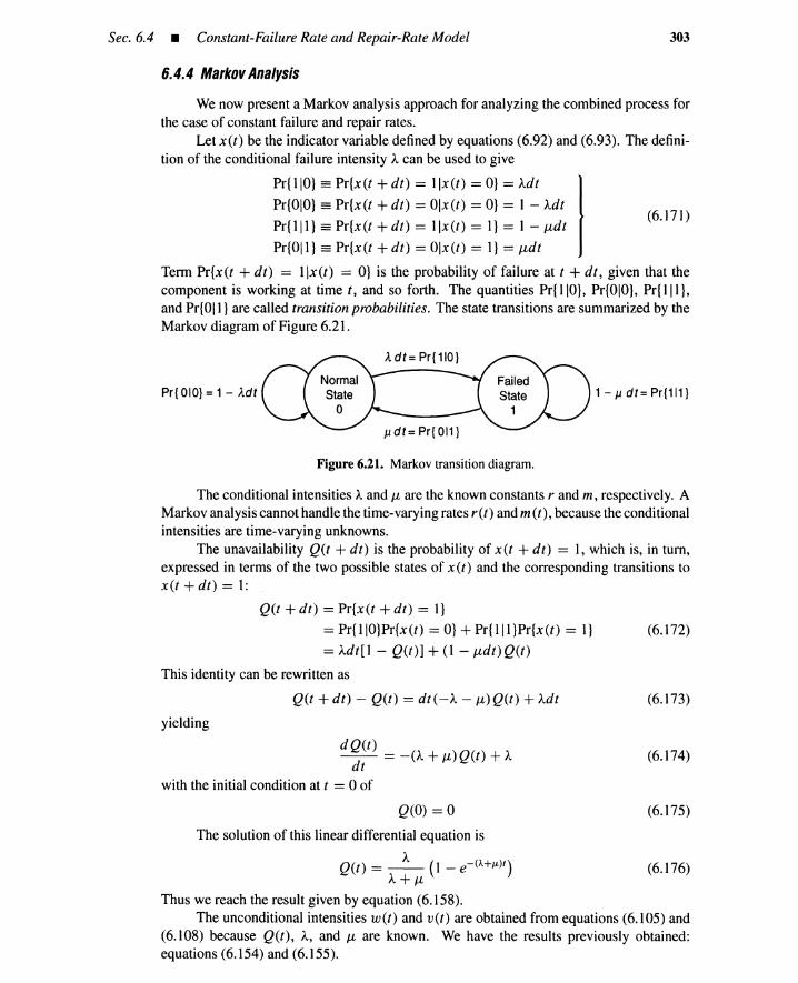
Sec. 6.4 • Constant-Failure Rate and Repair-Rate Model
6.4.4 Markov Analysis
303
(6.17] )
We now present a Markov analysis approach for analyzing the combined process forthe case of constant failure and repair rates.
Let x(t) be the indicator variable defined by equations (6.92) and (6.93). The defini-tion of the conditional failure intensity Acan be used to give
Pr{IIO} == Pr{x(t + dt) = Ilx(t) = O} = Adt
Pr{OIO} == Pr{x(t + dt) = Olx(t) = O} = 1 - Adt
Pr{Ill} == Pr{x (t + dt) = 11x (t) = I} = 1 - JLdt
Pr{OII} == Pr{x(t + dt) = Olx(t) = I} = udt
Term Pr{x(t + dt) = llx(t) = O} is the probability of failure at t + dt , given that thecomponent is working at time t, and so forth. The quantities Pr{110}, Pr{OIO}, Pr{Ill},and Pr{OII} are called transition probabilities. The state transitions are summarized by theMarkov diagram of Figure 6.21.
Pr{ OIO} = 1 - Adt
J1dt=Pr{OI1}
Figure 6.21. Markovtransition diagram.
1 - J1 d t=Pr{111 }
The conditional intensities Aand JL are the known constants rand m, respectively. AMarkov analysis cannot handle the time-varying rates r(t) and m(t), because the conditionalintensities are time-varying unknowns.
The unavailability Q(t + dt) is the probability of x(t + dt) = 1, which is, in tum,expressed in terms of the two possible states of x (t) and the corresponding transitions tox(t+dt)=I:
Q(t + dt) = Pr{x(t + dt) = I}
= Pr{IIO}Pr {x (t) = O} + Pr{Ill}Pr {x (t) = I}
= Adt[I - Q(t)] + (1 - udt) Q(t)
This identity can be rewritten as
Q(t + dt) - Q(t) = dt( -A - JL) Q(t) + Adt
yielding
dQ(t) = -(A + JL)Q(t) + Adt
with the initial condition at t = 0 of
Q(O) = 0
(6.172)
(6.173)
(6.174)
(6.175)
The solution of this linear differential equation is
AQ(t) =-- (1 - e-(A+JL)I) (6.176)
A+JL
Thus we reach the result given by equation (6.158).The unconditional intensities w(t) and v(t) are obtained from equations (6.105) and
(6.108) because Q(t), A, and JL are known. We have the results previously obtained:equations (6.154) and (6.155).
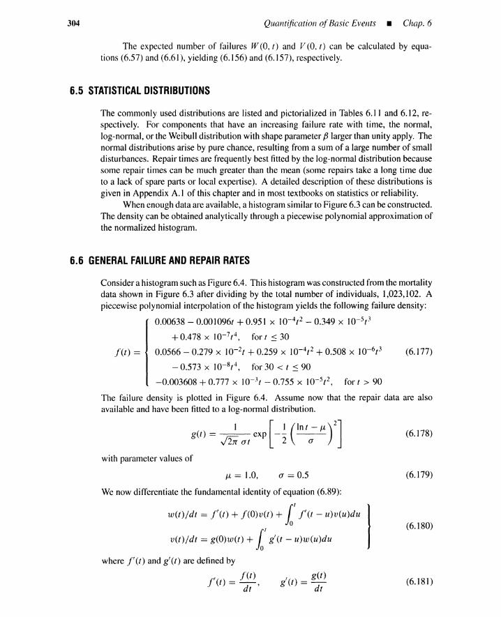
304 Quantification ofBasic Events - Chap. 6
The expected number of failures W (0, t) and V (0, t) can be calculated by equa-tions (6.57) and (6.61), yielding (6.156) and (6.157), respectively.
6.5 STATISTICAL DISTRIBUTIONS
The commonly used distributions are listed and pictorialized in Tables 6.11 and 6.12, re-spectively. For components that have an increasing failure rate with time, the normal,log-normal, or the Weibulldistribution with shape parameter f3 larger than unity apply. Thenormal distributions arise by pure chance, resulting from a sum of a large number of smalldisturbances. Repair times are frequently best fitted by the log-normal distribution becausesome repair times can be much greater than the mean (some repairs take a long time dueto a lack of spare parts or local expertise). A detailed description of these distributions isgiven in Appendix A.I of this chapter and in most textbooks on statistics or reliability.
When enough data are available, a histogram similar to Figure 6.3 can be constructed.The density can be obtained analytically through a piecewise polynomial approximation ofthe normalized histogram.
6.6 GENERAL FAILURE AND REPAIR RATES
Consider a histogram such as Figure 6.4. This histogram wasconstructed from the mortalitydata shown in Figure 6.3 after dividing by the total number of individuals, 1,023,102. Apiecewise polynomial interpolation of the histogram yields the following failure density:
0.00638 - 0.00 I096t + 0.951 x 10⁻⁴/ 2 - 0.349 x 10⁻⁵t 3
+0.478 x 10⁻⁷t 4 , fort:::; 30
j'(t) == 0.0566 - 0.279 x 10⁻²t + 0.259 x 10⁻⁴t2 + 0.508 x 10⁻⁶/ 3 (6.177)
- 0.573 x 10⁻⁸t 4 , for 30 < t ~ 90
-0.003608+0.777 x 10⁻³t -0.755 x 10⁻⁵/ 2 , fort> 90
The failure density is plotted in Figure 6.4. Assume now that the repair data are alsoavailable and have been fitted to a log-normal distribution.
[ ( )2]I I In/ - J.lg(t) == r;:c exp --
v2Jr at 2 a
with parameter values of
(6.178)
J.l == 1.0, a == 0.5 (6.179)
Ii (I) = g(/)d/
We now differentiate the fundamental identity of equation (6.89):
w(/)/dl = f'(/) + f(O)v(t) + it r« - u)v(u)du
v(/)/dl = g(O)W(/) + it g'(1 - u)w(u)du
where j" (t) and g' (t) are defined by
f'(/) = fd;),
(6.180)
(6.181)
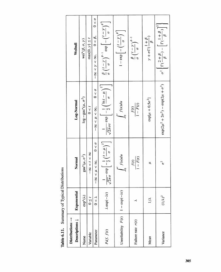
~ 5i
Tab
le6.
11.
Sum
mar
yof
Typ
ical
Dis
trib
utio
ns
Dis
trib
utio
ns-+
Des
crip
tion
sI
Exp
onen
tial
Nor
mal
Log
-Nor
mal
Wei
bull
Nam
eex
p*(A
)ga
u*(J
L,a
2)
log
- gau
*(JL
,a
2)
wei
*({3
,a,
y)
Var
iabl
eO~t
-0
0<
t<
00
O<
tm
ax{O
,y}
~t
Par
amet
erO
<A
-0
0<
JL<
00
,O
<a
-0
0<
JL<
00
,O
<a
-0
0<
y<
00
,o
<{3
,O
<a
ra].
ol(t
)A
exp
(-A
t)1
[1C-
JLf]
1[1
Cot-J
LY]
Pc-
yr-I
[C-y
)P]
-Jii
aex
p-2
"-a
----
exp
--
---
---
exp
---
-Jii
at
2a
aa
a
Unr
elia
bili
tyF
(t)
1-
exp
(-A
t)l'f
(u)d
ul'f
(u)d
ul-
exp[
-C~Y
)P]
Fai
lure
rate
r(t)
AjO
(t)n»
~c~yr-I
1-
F(t
)1
-F
(t)
Mea
nI/
Aex
plu
+0
.5a
2]
I+{
3JL
y+
ar(--)
{3
Var
ianc
e(I
/A)2
a2
exp(
2JL
2+
2a2
)-
exp(
2JL
+a
2)
a2[1(
2;p)-
[I(I;p
)rl
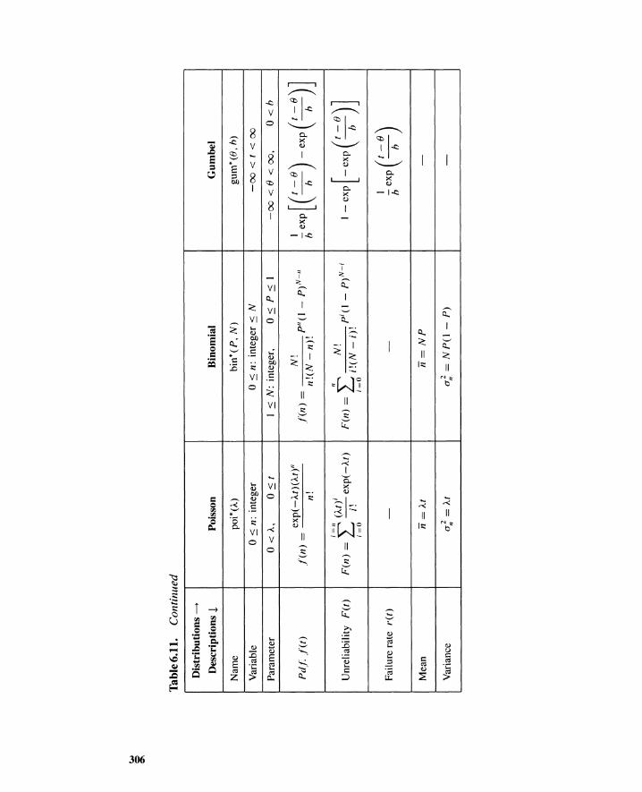
~ ~
Tab
le6.
11.
Con
tinu
ed
Dis
trib
utio
ns~
Des
crip
tion
sI
Nam
e
Var
iabl
e
Poi
sson
poi*
(A)
o:s
n:in
tege
r
Bin
omia
l
bin
*(P
,N
)
o:s
n:in
tege
r:s
N
Gu
mb
el
gum
*(O
,h)
-0
0<
t<
00
Par
amet
er0
<A
,o
:st
I::s
N:
inte
ger,
O:s
P:s
I-0
0<°<
00
,O
<h
Pd
f:.l
(t)
Unr
elia
bili
tyF
(t)
Fai
lure
rate
r(t)
Mea
n
Var
ianc
e
f'( n
)=
exp(
- At)
( At)
"
n!
i=1I
(At)
iF
(n)
=L
-.,-e
xp
(-A
t)i=
()I.
11=
At
a,;=
At
.N
!f(
n)
=P
Il(1
_p
) N- 1
ln
!(N
-n)!
IIN
'F
(n)
=L
.p
i(l
-ri
":'
i=()
i!(N
-i)
!
11=
NP
a,;=
NP
(I-
P)
1[(t
-O)
(t-O
)]h
exp
-h
--
exp
-h
-
I-
exp
[-
expC~
e)]
I(t
-0)
hex
p-h
-

YJ
Q '-I
Tab
le6.
11.
Con
tinu
ed
Dis
trib
utio
ns~
Des
crip
tion
s1
Inve
rse
Gau
ssia
nG
amm
aB
eta
Nam
ein
v-
gau*
(p, k
)ga
m*(
/3,
Y/)
beta
*(a,
/3)
Var
iabl
eo
<t
o<
tO
<x<
1
Par
amet
erp
=1=
0,O
<k
0<
/3,
O<
y/
-I
<a,
- 1<
/3
(_ky
/ 2ex
p[
-kp(t
_~)2]
(r-I
'(x
-re
a+
/3+
2)x
a1
_x
f3P
d,l
,l(t
)1
t-f
/1]
2rr
pt3
2ty/
r(/3
)~
ej
()
-r
(a+
1)r
(/3+
I)(
)
Unr
elia
bili
tyF
(t)
l'f(u
)du
l'f(u
)du
F(x
)=lx
f(u
)du
Fai
lure
rate
r(t)
j'(t
).l
(t)
()
f(x)
rx
=1
-F
(t)
1-
F(t
)I
-F
(x)
Mea
nt
=lip
Y//3
(a+
I)/(
a+
/3+
2)
Var
ianc
ea/
=I/
(kp2
)y/
2/3
2(a
+I)
(/3+
1)a
=x
(a+
/3+
2)2
(a+
/3+
3)
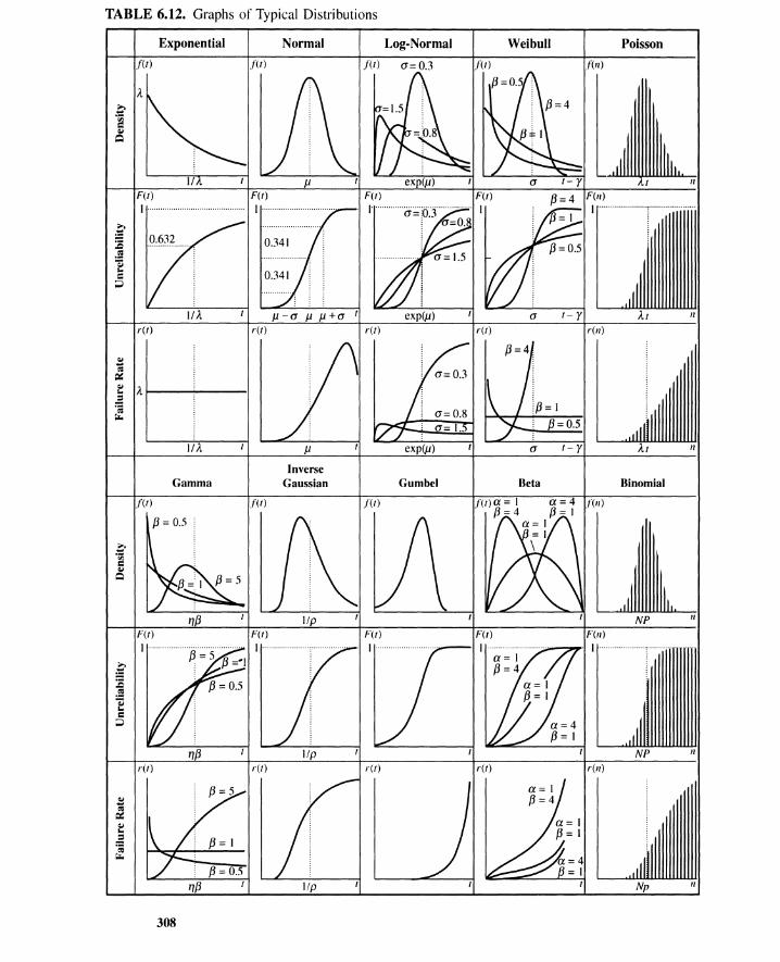
TABLE 6.12. Graphs of Typical Distributions
Exponential Normal Log-Normal Weibull Poisson
f(t) f(t) f(t) a= 0.3 f(l1)
A~...o~
QIQ
II J.l 11
F(t) F(t)I········..···· ............·..·..··..........· I·......··..............·......··· ..
~
== 0.341:E0$~r..C
;;)
J.l-a J.l J.l+a t exp(u) a t-y At 11
r(t) r(t) r(t) r(t) rtn)
QI
=~QI A-.a 1/3 = I0;"'- /3 =0.5
I/A J.l exp(u) a t- r 11
InverseGamma Gaussian Gumbel Beta Binomial
f(t) /(t) f(l1)
~o~
CQI
Q
NP 11
F(t) F(I1)I·.... ···· ..............··.... I
~:E.s~-c;;)
IIp NP 11
r(t) r(t) r(t) r(t) r(l1)
~~
~~r...a0;"'-
IIp Np 11
308

Sec. 6.7 • Estimating Distribution Parameters 309
The differential equation (6.180) is now integrated, yielding w(t) and v(t). The expectednumber of failures W(O, t) and repairs V(O, t) can be calculated by integration of equa-tions (6.57) and (6.61). The unavailability Q(t) is given by equation (6.96). The conditionalfailure intensity A(t) can be calculated by equation (6.106). Given failure and repair den-sities, the probabilistic parameters for any process can be obtained in this manner.
6.7 ESTIMATING DISTRIBUTION PARAMETERS
Given sufficient data, a histogram such as Figure 6.4 can be constructed and the failure orrepair distribution determined by a piecewise polynomial approximation, as demonstratedin Section 6.6. The procedure of Figure 6.16 is then applied, and the probabilistic conceptsare quantified.
When only fragmentary data are available we cannot construct the complete his-togram. In such a case, an appropriate distribution must be assumed and its parametersevaluated from the data. The component quantification can then be made using the flowchart of Figure 6.16.
In this section, parameter estimation (or identification) methods for the repair-to-failure and the failure-to-repair process are presented.
6.7.1 Parameter Estimation forRepair-to-Failure Process
In parameter estimation based on test data, three cases arise:
1. All components concerned proceed to failure and no component is taken out ofuse before failure. (All samples fail.)
2. Not all components being tested proceed to failure because they have been takenout of service before failure. (Incomplete failure data.)
3. Only a small portion of the sample is tested to failure. (Early failure data.)
Case1: Allsamples/ail. Consider the failure data for the 250germanium transistorsin Table 6.5. Assume a constant failure rate A. The existence ofthe constant Acan be checkedas follows.
The survival distribution is given by
R(t) == «:" (6.182)
This can be written as
In [_1_] == At (6.183)R(t)
So, if the natural In of 1j R(t) is plotted against t, it should be a straight line with slope A.Values of In[ljR(t)] versus t from Table 6.5 are plotted in Figure 6.22. The best
straight line is passed through the points and the slope is readily calculated:
A = Y2 - Yl = 1.08 - 0.27 = 0.0027 (6.184)X2-XI 400-100
Note that this A is consistent with constant rate r == 0.0026 in Example 3.
Case2: Incompletefailure data. In some tests, components are taken out of servicefor reasons other than failures. This will affect the number of components exposed to failure
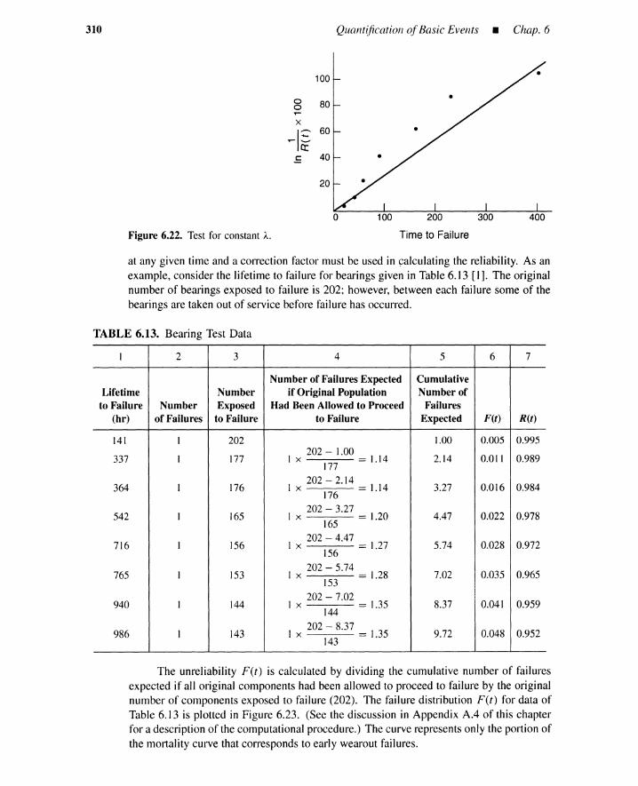
310 Quantification ofBasic Events - Chap. 6
Figure 6.22. Test for constant A.
100
0 800~
x
~I~60
.f: 40
20
0 100 200
Time to Failure
400
at any given time and a correction factor must be used in calculating the reliability. As anexample, consider the lifetime to failure for bearings given in Table 6.13 [1]. The originalnumber of bearings exposed to failure is 202; however, between each failure some of thebearings are taken out of service before failure has occurred.
TABLE 6.13. Bearing Test Data
I 2 3 4 5 6 7
Number of Failures Expected CumulativeLifetime Number if Original Population Number of
to Failure Number Exposed Had Been Allowed to Proceed Failures(hr) of Failures to Failure to Failure Expected F(t) R(t)
141 1 202 1.00 0.005 0.995202-1.00
2.14 0.011 0.989337 I 177 I x = 1.14177
176202 - 2.14
3.27 0.016 0.984364 I Ix = 1.14176
202 - 3.274.47 0.022 0.978542 I 165 Ix = 1.20
165202 - 4.47
0.028 0.972716 I 156 Ix = 1.27 5.74156
202 - 5.74 = 1.28 7.02 0.035 0.965765 I 153 Ix153
202 - 7.020.041 0.959940 I 144 Ix = 1.35 8.37
144
202 - 8.37 = 1.35 9.72 0.048 0.952986 I 143 Ix143
The unreliability F(t) is calculated by dividing the cumulative number of failuresexpected if all original components had been allowed to proceed to failure by the originalnumber of components exposed to failure (202). The failure distribution F(t) for data ofTable 6.13 is plotted in Figure 6.23. (See the discussion in Appendix A.4 of this chapterfor a description of the computational procedure.) The curve represents only the portion ofthe mortality curve that corresponds to early wearout failures.
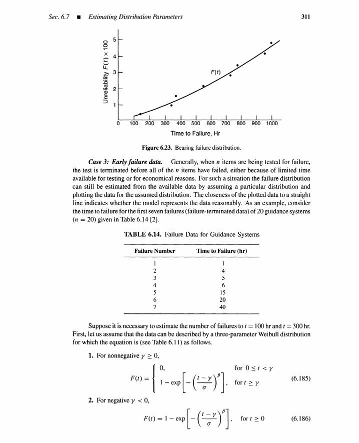
Sec. 6.7 • Estimating Distribution Parameters 311
0 50~
x 4...-.......i:L~
3
:0.~ 2CD~
c:::::>
a 100 200 300 400 500 600 700 800 900 1000
Time to Failure, Hr
Figure 6.23. Bearing failure distribution.
Case 3: Earlyfailure data. Generally, when n items are being tested for failure,the test is terminated before all of the n items have failed, either because of limited timeavailable for testing or for economical reasons. For such a situation the failure distributioncan still be estimated from the available data by assuming a particular distribution andplotting the data for the assumed distribution. The closeness of the plotted data to a straightline indicates whether the model represents the data reasonably. As an example, considerthe time to failure for the first seven failures (failure-terminated data) of20 guidance systems(n == 20) given in Table 6.14 [2].
TABLE 6.14. Failure Data for Guidance Systems
Failure Number
1234
567
Time to Failure (hr)
1456152040
Suppose it is necessary to estimate the number of failures to t == 100 hr and t == 300 hr.First, let us assume that the data can be described by a three-parameter Weibull distributionfor which the equation is (see Table 6.11) as follows.
1. For nonnegative y ~ 0,
F(t)=={ 0, [(t-y)fJ]l-exp - -- ,
a
for 0 ::s t < Y
for t ~ Y(6.185)
2. For negative y < 0,
F(t) = 1 - exp [ - C~ yrl for t ~ 0 (6.186)
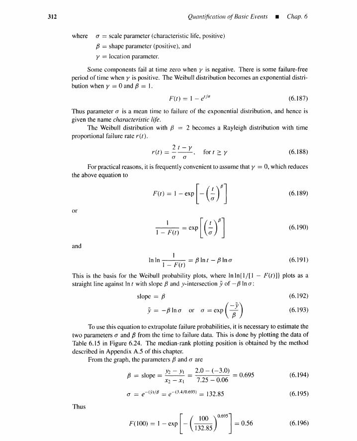
312 Quantification ofBasic Events - Chap. 6
where a == scale parameter (characteristic life, positive)
fJ == shape parameter (positive), and
y == location parameter.
Some components fail at time zero when y is negative. There is some failure-freeperiod of time when y is positive. The Weibull distribution becomes an exponential distri-bution when y == 0 and fJ == I.
F (t) == I - e'/a (6.187)
Thus parameter a is a mean time to failure of the exponential distribution, and hence isgiven the name characteristic life.
The Weibull distribution with fJ == 2 becomes a Rayleigh distribution with timeproportional failure rate rtt).
2 t - Yret) == ---, fort ~ y
a a(6.188)
For practical reasons, it is frequently convenient to assume that y == 0, which reducesthe above equation to
or
and
I - IF(t) = exp [ (~r]
(6.189)
(6.190)
(6.192)
(6.] 93)
IInln ==fJlnt-fJlna (6.191)
I - F(t)
This is the basis for the Weibull probability plots, where InIn{lj[1 - F(t)]} plots as astraight line against In t with slope fJ and y-intersection 5; of - fJ Ina:
slope == fJ
Y = -filna or a =exp (1)To use this equation to extrapolate failure probabilities, it is necessary to estimate the
two parameters a and fJ from the time to failure data. This is done by plotting the data ofTable 6.15 in Figure 6.24. The median-rank plotting position is obtained by the methoddescribed in Appendix A.5 of this chapter.
From the graph, the parameters fJ and a are
Thus
V2 - VI 2.0 - (-3.0)fJ == slope == --'--'- == == 0.695
X2 - Xl 7.25 - 0.06
a == e-Cv)/fJ == e-(3.4jO.695) == 132.85
[ (100 )0.695]
F(100) == I - exp - -- == 0.56132.85
(6.] 94)
(6.195)
(6.196)
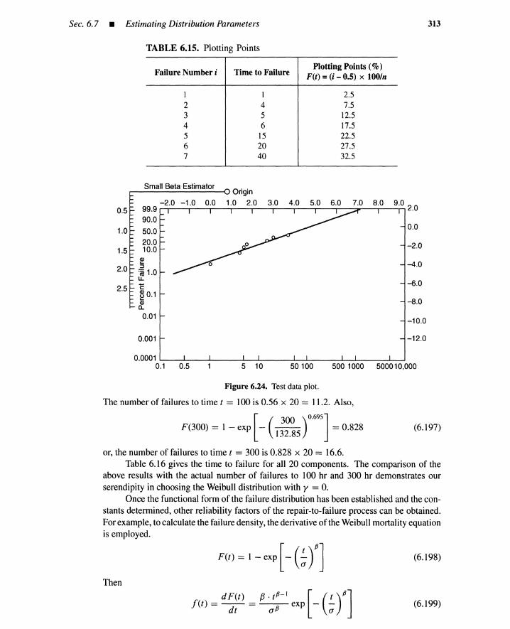
Sec. 6.7 • Estimating Distribution Parameters 313
TABLE 6.15. Plotting Points
Failure Number i Time to FailurePlotting Points (%)
F(t) =(i - 0.5) x 100/n
1234567
1456
152040
2.57.5
12.517.522.527.532.5
500 1000 500010,000
0.0
-10.0
-4.0
-6.0
-8.0
-12.0
-2.0
7.0 8.0 9.0 2.0
50100
3.0 4.0 5.0 6.0
5 10
Origin1.0 2.0
Small Beta Estimator
-2.0 -1.0 0.099.990.0
50.020.010.0
Q)
:;~ 1.0LL
'E~ 0.1CDa..0.01
0.001
0.0001 ~_.....L-_---a-__---L._..L.-..__--L----'--__---'-_.L..--__..L.-""""
0.1 0.5
0.5
2.0
2.5
1.0
1.5
Figure 6.24. Test data plot.
(6.197)
The number of failures to time t == 100 is 0.56 x 20 == 11.2. Also,
[ (300 )0.695]
F(300) == 1 - exp - 132.85 == 0.828
or, the number of failures to time t == 300 is 0.828 x 20 == 16.6.Table 6.16 gives the time to failure for all 20 components. The comparison of the
above results with the actual number of failures to 100 hr and 300 hr demonstrates ourserendipity in choosing the Weibull distribution with y == O.
Once the functional form of the failure distribution has been established and the con-stants determined, other reliability factors of the repair-to- failure process can be obtained.For example, to calculate the failure density, the derivative of the Weibull mortality equationis employed.
F(t) = 1- exp [ - (~r] (6.198)
Then
dF(t) fJ . t fJ -1
[( t )fJ]f(t) == -- == exp - -dt a fJ a
(6.199)

314 Quantification ofBasic Events _ Chap. 6
TABLE 6.16. More Data for Guidance System
Failure Number Time to Failure (hr) Failure Number Time to Failure (hr)
I I II 952 4 12 1063 5 13 1254 6 14 1515 15 15 2006 20 16 2687 40 17 4598 41 18 8279 60 19 840
10 93 20 1089
Substituting values for a and fJ gives
, 0.02324 [( t ) 0.695]/ (t) == to.305 exp - 132.85 (6.200)
The calculated values of /'(t) are given in Table 6.17 and plotted in Figure 6.25. Thesevalues represent the probability that the first component failure occurs per unit time at timet , given that the component was operating as good as new at time zero.
TABLE 6.17. Failure Density for Guidance System
Time to Failure Time to Failure(hr) f(l) (hr) f(l)
1 0.0225 95 0.00264 0.0139 106 0.00245 0.0128 125 0.00206 0.0120 151 0.0017
15 0.0082 200 0.001220 0.0071 268 0.000840 0.0049 459 0.000340 0.0049 827 0.000160 0.0037 840 -
93 0.0027 1089 -
The expected number of times the failures occur in the interval t to t +dt is w(t )dt,and its integral over an interval is the expected number of failures. Once the failure densityand the repair density are known, the unconditional failure intensity w(t) may be obtainedfrom equation (6.89).
Assume that the component is as good as new at time zero. Assume further that oncethe component fails at time t > 0 it cannot be repaired (nonrepairable component). Thenthe repair density is identically equal to zero, and the unconditional repair intensity v(t) ofequation (6.89) becomes zero. Thus
. 0.02324 [( t )0.695]w(t) == j (t) == to.305 exp - 132.85 (6.201 )
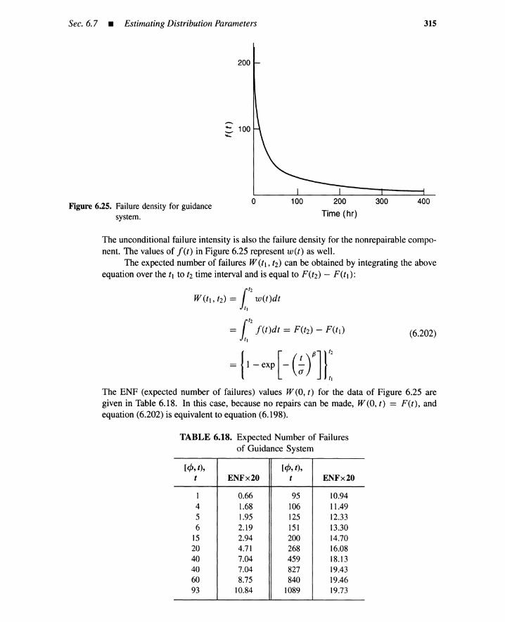
Sec. 6.7 • Estimating Distribution Parameters 315
Figure 6.25. Failure density for guidancesystem.
o 100 200
Time (hr)
300 400
The unconditional failure intensity is also the failure density for the nonrepairable compo-nent. The values of f(/) in Figure 6.25 represent w(/) as well.
The expected number of failures W(11, (2) can be obtained by integrating the aboveequation over the 11 to 12 time interval and is equal to F(/2) - F(/l):
(6.202)
The ENF (expected number of failures) values W(O, t) for the data of Figure 6.25 aregiven in Table 6.18. In this case, because no repairs can be made, W(O, t) = F(/), andequation (6.202) is equivalent to equation (6.198).
TABLE 6.18. Expected Number of Failuresof Guidance System
[cP, t), [cP, t),t ENFx20 t ENFx20
1 0.66 95 10.944 1.68 106 11.495 1.95 125 12.336 2.19 151 13.30
15 2.94 200 14.7020 4.71 268 16.0840 7.04 459 18.1340 7.04 827 19.4360 8.75 840 19.4693 10.84 1089 19.73
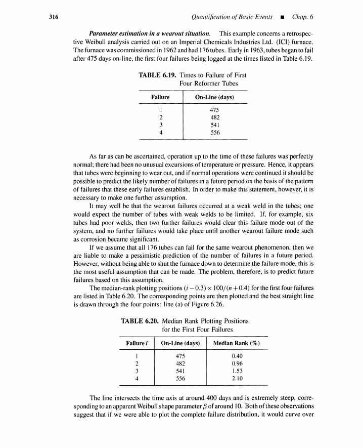
316 Quantification ofBasic Events _ Chap. 6
Parameter estimation in a wearout situation. This example concerns a retrospec-tive Weibull analysis carried out on an Imperial Chemicals Industries Ltd. (ICI) furnace.The furnace was commissioned in 1962 and had 176 tubes. Early in 1963, tubes began to failafter 475 days on-line, the first four failures being logged at the times listed in Table 6.19.
TABLE 6.19. Times to Failure of FirstFour Reformer Tubes
Failure
1234
On-Line (days)
475482541556
As far as can be ascertained, operation up to the time of these failures was perfectlynormal; there had been no unusual excursions of temperature or pressure. Hence, it appearsthat tubes were beginning to wear out, and if normal operations were continued it should bepossible to predict the likely number of failures in a future period on the basis of the patternof failures that these early failures establish. In order to make this statement, however, it isnecessary to make one further assumption.
It may well be that the wearout failures occurred at a weak weld in the tubes; onewould expect the number of tubes with weak welds to be limited. If, for example, sixtubes had poor welds, then two further failures would clear this failure mode out of thesystem, and no further failures would take place until another wearout failure mode suchas corrosion became significant.
If we assume that all 176 tubes can fail for the same wearout phenomenon, then weare liable to make a pessimistic prediction of the number of failures in a future period.However, without being able to shut the furnace down to determine the failure mode, this isthe most useful assumption that can be made. The problem, therefore, is to predict futurefailures based on this assumption.
The median-rank plotting positions (i - 0.3) x 100/(n +0.4) for the first four failuresare listed in Table 6.20. The corresponding points are then plotted and the best straight lineis drawn through the four points: line (a) of Figure 6.26.
TABLE 6.20. Median Rank Plotting Positionsfor the First Four Failures
Failure i On-Line (days) Median Rank (%)
1 475 0.402 482 0.963 541 1.534 556 2.10
The line intersects the time axis at around 400 days and is extremely steep, corre-sponding to an apparent Weibull shape parameter fJ of around 10. Both of these observationssuggest that if we were able to plot the complete failure distribution, it would curve over
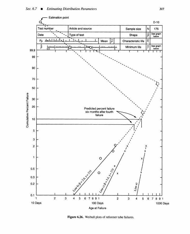
Sec. 6.7 • EstimatingDistribution Parameters 317
xI
x
5 6 7 8 9 1
1000 Days
43
0-10
Sample size N 176
Shape1\ Seegraphf3 below
Characteristic life1\11
Minimum life1\ Seegraphr below
2
Predicted percent failuresix months after fourth
failure
,,,,,,,,,,,,
, , , , , , , , , , , , , , , , , , , , , , , , , ,, I
" I, I
, I
" I, I
" I, I
, I
" I, I
, I
~/, I,
4567891
100 Days
Age at Failure
Article and source
32
, , , ' , , Type of test
,I I " , I , , , , , , I 116:! ' ,,,,,,, I rive' , " , I , I I , , " , I I I
0.5 1 2 3' 4 5
,I",I,II,I,I'~J ' I I' L '
, Estimation point
~,
"Test number
1
10 Days
0.1
0.5
0.3
0.2
Date
P,u1\
f399.9
99
90
70
50
Q)
~.(ij 30u..'EQ)
20eQ)Q..Q)
>~ 10"5E::Jo
5
3
2
Figure 6.26. Weibull plots of reformer tube failures.

318 Quantification ofBasic Events - Chap. 6
toward the time axis as failures accumulated, indicating a three-parameter Weibull modelrather than the simplest two-parameter model that can be represented by a straight line onthe plotting paper.
From the point of view of making predictions about the future number of failures, astraight line is clearly easier to deal with than a small part of a line of unknowncurvature.Physically, the three-parameterWeibull model
F(t) == II -exp [- c:yrl0,
for t ~ Y ~ 0
for 0 :::: t < Y
(6.203)
(6.204)
implies that no failure occurs during the initial period [0, y). Similar to equation (6.191),we have for t ~ y,
IInIn == tJ In(t - y) - tJ Ina
I - F(t)
Thus mathematically, the Weibull model can be reduced to the two-parametermodel and isrepresented by a straight line by making the transformation
t' == t - y (6.205)
Graphically, this is equivalent to plotting the failure data with a fixed time subtracted fromthe times to failure.
The correct time has been selected when the transformed plot
{ In(t - y), InIn [ I ] }I - F(t)
becomes the asymptote of the final part of the original curved plot
{In i, InIn [ I ] }I - F(t)
(6.206)
(6.207)
because Int ~ In(t - y) for large values of t.
In this case it is impossible to decide empirically what the transformation shouldbe because only the initial part of the curved plot is available. However, we are dealingwith a wearout phenomenon, and from experience we know that when these phenomenaare represented by a two-parameterWeibull model, the Weibull shape parameter generallytakes a value 2 S tJ :::: 3.4. Hence fixed times are subtracted from the four times to failuresuntil, by trial and error, the straight lines drawn through the plotted points have apparentvalues of tJ of 2 and 3.4. These are, respectively, lines (b) and (c) of Figure 6.26. Thetransformation formed by trial and error is shown in Table 6.21.
In Figure 6.26, the two lines havebeen projected forward to predict the likely numberof failures in the six monthsafter the fourth failure (i.e., to 182days after the fourth failure).The respective predictions are of 9 and 14 further failures.
The furnace was, in fact, operated for more than six months after the fourth failureand, in the six-month period referred to, 11 further failures took place.
6.7.2 Parameter Estimation for Failure-to-Repair Process
Time to repair (TTR), or downtime, consists not only of the time it takes to repaira failure but also of waiting time for spare parts, personnel, and so on. The availability
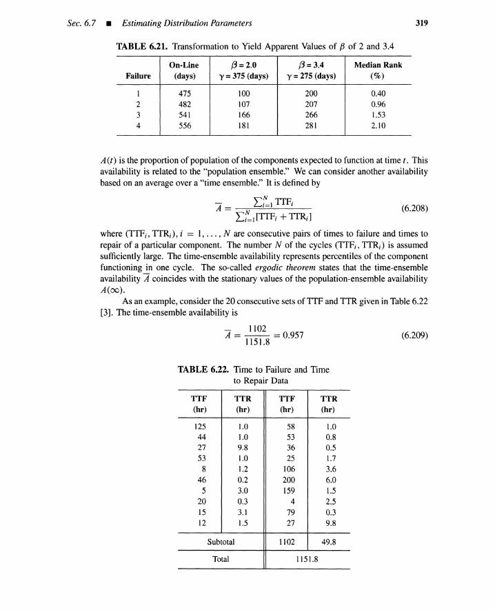
Sec. 6.7 • Estimating Distribution Parameters
TABLE 6.21. Transformation to Yield Apparent Values of f3 of 2 and 3.4
On-Line 13 =2.0 13 =3.4 Median RankFailure (days) y =375 (days) y =275 (days) (%)
1 475 100 200 0.402 482 107 207 0.963 541 166 266 1.534 556 181 281 2.10
319
(6.208)
(6.209)
A (t) is the proportion of population of the components expected to function at time t. Thisavailability is related to the "population ensemble." We can consider another availabilitybased on an average over a "time ensemble." It is defined by
A = 'L~l TIF;'L:I[TTFj +TTRj ]
where (TTF j , TTR j ) , i = 1, ... , N are consecutive pairs of times to failure and times torepair of a particular component. The number N of the cycles (TTFj , TTRj ) is assumedsufficiently large. The time-ensemble availability represents percentiles of the componentfunctioning in one cycle. The so-called ergodic theorem states that the time-ensembleavailability A coincides with the stationary values of the population-ensemble availabilityA(oo).
As an example, consider the 20 consecutive sets of TTF and TTR given in Table 6.22[3]. The time-ensemble availability is
- 1102A = -- =0.957
1151.8
TABLE 6.22. Time to Failure and Timeto Repair Data
TTF TTR TTF TTR(hr) (hr) (hr) (hr)
125 1.0 58 1.044 1.0 53 0.827 9.8 36 0.553 1.0 25 1.78 1.2 106 3.6
46 0.2 200 6.05 3.0 159 1.5
20 0.3 4 2.515 3.1 79 0.312 1.5 27 9.8
Subtotal 1102 49.8
Total 1151.8
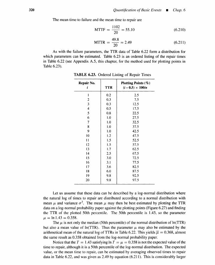
320 Quantification ofBasic Events - Chap. 6
The mean time to failure and the mean time to repair are
1102MTTF == - == 55.10
20
49.8MTTR == - == 2.49
20
(6.210)
(6.211)
As with the failure parameters, the TTR data of Table 6.22 form a distribution forwhich parameters can be estimated. Table 6.23 is an ordered listing of the repair timesin Table 6.22 (see Appendix A.5, this chapter, for the method used for plotting points inTable 6.23).
TABLE 6.23. Ordered Listing of Repair Times
Repair No. Plotting Points (%)i TTR (i - 0.5) x lOO/n
I 0.2 2.52 0.3 7.53 0.3 12.54 0.5 17.55 0.8 22.56 1.0 27.57 1.0 32.58 1.0 37.59 1.0 42.5
10 1.2 47.5II 1.5 52.512 1.5 57.513 1.7 62.514 2.5 67.515 3.0 72.516 3.1 77.517 3.6 82.518 6.0 87.519 9.8 92.520 9.8 97.5
Let us assume that these data can be described by a log-normal distribution wherethe natural log of times to repair are distributed according to a normal distribution withmean J.1 and variance a 2• The mean J.1 may then be best estimated by plotting the TTRdata on a log-normal probability paper against the plotting points (Figure 6.27) and findingthe TTR of the plotted 50th percentile. The 50th percentile is 1.43, so the parameterJ.1 == In 1.43 == 0.358.
The J.1 is not only the median (50th percentile) of the normal distribution of In(TTR)but also a mean value of In(TTR). Thus the parameter J.1 may also be estimated by thearithmetical mean of the natural log of TTRs in Table 6.22. This yields Ii == 0.368, almostthe same result as 0.358 obtained from the log-normal probability paper.
Notice that the T == 1.43 satisfying In T == J.1 == 0.358 is not the expected value of thetime to repair, although it is a 50th percentile of the log-normal distribution. The expectedvalue, or the mean time to repair, can be estimated by averaging observed times to repairdata in Table 6.22, and was given as 2.49 by equation (6.211). This is considerably larger
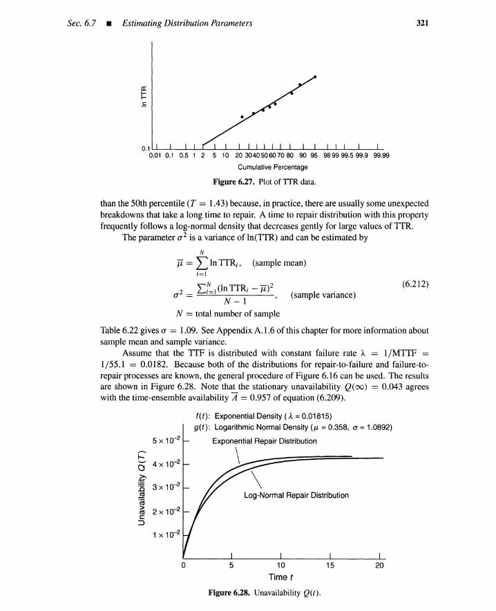
Sec. 6.7 • Estimating Distribution Parameters 321
0.1 L....I---.a.._-'--~_""---'""----'----'--""---L-""-"""""----'---""----'----I~-..L----IL....-..--'--
0.01 0.1 0.5 1 2 5 10 20 3040506070 80 90 95 9899 99.5 99.9 99.99
Cumulative Percentage
Figure 6.27. Plot ofTTR data.
than the 50th percentile (T = 1.43) because, in practice, there are usually some unexpectedbreakdowns that take a long time to repair. A time to repair distribution with this propertyfrequently follows a log-normal density that decreases gently for large values of TTR.
The parameter a 2 is a variance of In(TTR) and can be estimated by
N
Ji = L InTTR;, (sample mean);=1
(6.212)2 2:::1 (In TTR; - Ji)2a = N _ 1 (sample variance)
N = total number of sample
Table 6.22 gives a = 1.09. See Appendix A.1.6 of this chapter for more information aboutsample mean and sample variance.
Assume that the TTF is distributed with constant failure rate A = 1/MTTF =1/55.1 = 0.0182. Because both of the distributions for repair-to-failure and failure-to-repair processes are known, the general procedure of Figure 6.16 can be used. The resultsare shown in Figure 6.28. Note that the stationary unavailability Q( (0) = 0.043 agreeswith the time-ensemble availability A = 0.957 of equation (6.209).
2015
Log-Normal Repair Distribution
5 10
Time t
Figure 6.28. Unavailability Q(t).
f(t): Exponential Density (A = 0.01815)
g(t): Logarithmic Normal Density (/l = 0.358, a = 1.0892)
Exponential Repair Distribution
\
o
5 X 10⁻²
1 X 10⁻²
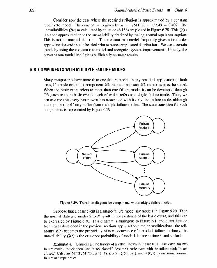
322 Quantification ofBasic Events _ Chap. 6
Consider now the case where the repair distribution is approximated by a constantrepair rate model. The constant m is given by m == I/MTTR == 1/2.49 == 0.402. Theunavailabilities Q(t) as calculated by equation (6.158) are plotted in Figure 6.28. This Q(t)
is a good approximation to the unavailability obtained by the log-normal repair assumption.This is not an unusual situation. The constant rate model frequently gives a first-orderapproximation and should be tried prior to more complicated distributions. Wecan ascertaintrends by using the constant rate model and recognize system improvements. Usually, theconstant rate model itself gives sufficiently accurate results.
6.8 COMPONENTS WITH MULTIPLE FAILURE MODES
Many components have more than one failure mode. In any practical application of faulttrees, if a basic event is a component failure, then the exact failure modes must be stated.When the basic event refers to more than one failure mode, it can be developed throughOR gates to more basic events, each of which refers to a single failure mode. Thus, wecan assume that every basic event has associated with it only one failure mode, althougha component itself may suffer from multiple failure modes. The state transition for suchcomponents is represented by Figure 6.29.
Figure 6.29. Transition diagram for components with multiple failure modes.
Suppose that a basic event is a single-failure mode, say mode 1 in Figure 6.29. Thenthe normal state and modes 2 to N result in nonexistence of the basic event, and this canbe expressed by Figure 6.30. This diagram is analogous to Figure 6.1, and quantificationtechniques developed in the previous sections apply without major modifications: the reli-ability R(t) becomes the probability of non-occurrence of a mode 1 failure to time t, theunavailability Q(t) is the existence probability of mode 1 failure at time t , and so forth.
Example 8. Consider a time history of a valve, shown in Figure 6.31. The valve has twofailure modes, "stuck open" and "stuck closed." Assume a basic event with the failure mode "stuckclosed." Calculate MTTF, MTTR, R(t), F(t), A(t), Qtt), w(t), and W(O, t) by assuming constantfailure and repair rates.

[82]
Sec. 6.8 • Components with Multiple Failure Modes
Mode 1 Occurs
Figure 6.30. Transition diagram for a basic event.
30 0.6 [106] (3.0)N - - - - -~ SO - - - - -~ N - - - - -~ SC - - - - -~ N
I
: [200]I
[159] 0.8 14 (0.3)'SC ......- - - - - N ......- - - - - SO ......- - - - - N ......- - - - - SC
I
(3.1) :I
, [4.5] (1.4) 18 0.7N - - - - -~ SC - - - - -~ N - - - - -~ SO - - - - -~ N
IIII
[28] 1.1 27 (1.0) ,SC ......- - - - - N ......- - - - - SO ......- - - - - N ......- - - - - SC
II
(1.7) II
, 89 2.1 [59] (0.8)N - - - - -~ SO - - - - -~ N - - - - -~ SC - - - - -~ N
Figure 6.31. A time history of a valve.
N : NormalSO : Stuck OpenSC : Stuck Closed
323
Solution: The "valve normal" and "valve stuck open" denote nonexistence of the basic event.Thus Figure 6.31 can be rewritten as Figure 6.32, where the symbol NON denotes the nonexistence.
136.6 + 200 + 173.8 + 4.5 + 100.7 + 56.1 + 150.1MTTF = = 117.4
7
MTTR = 3.0 + 0.3 + 3.1 + 1.4 + 1.0 + 1.7 + 0.8 = 1.61 (6.213)7
1 1A = MTTF = 0.0085, u. = MTTR = 0.619
Table 6.10 yields
F(t) = 1 - e-O.OO85t, R(t) = e-O.OO85t
0.0085Q(t) = [1 - e-(O.OO85+0.619)f]
0.0085 + 0.619
= 0.0135 x [1 - e-O.6275t]
A(t) = 0.9865 + 0.0135e-o.6275f
w(t = 0.0085 x 0.619 0.00852
1 _ e-(O.OO85+0.619)f
) 0.0085 + 0.619 + (0.0085 + 0.619) [ ]
= 0.0084 + 0.0001e-O.6275t
W(O t) = 0.0085 x 0.619 t 0.00852
1 _ e-(O.OO85+0.619)f
, 0.0085 + 0.619 + (0.0085 + 0.619)2 [ ]
= 0.0002 + 0.00841 - 0.0002e-O.6275t
(6.214)

324 Quantification ofBasic Events - Chap. 6
NON - _39:~·~:~~6__ ~ sc __ ~:.O__ • NON __ ~~O__ • SC 0:.3 ~ NON
: 14+0.8+159II
18+0.7+82 1.4 4.5 3.1 tSC ~ - - - - - - - - - - - NON • - - - - - - SC ...... - - - - - - NON • - - - - - - SC
1.0 :II
t 27+1.1+28 1.7 89 + 2.1 + 59 0.8NON - - - - - - - - - - - ~ SC- - - - - - • NON - - - - - - - - - - - ~ SC - - - - - -. NON
Figure 6.32. TTFs and TTRs of "stuck closed" event for the valve.
These calculations hold only approximately because the three-state valve is modeled by thetwo-statediagram of Figure6.32. However, MTTR for "stuck open" is usually small, and the approx-imation error is negligible. If rigorous analysis is required, we can start with the Markov transitiondiagram of Figure 6.33 and apply the differential equations described in Chapter 9 for the calculationof R(t), Qtt), w(t), and so on. •
o Normal
Figure 6.33. Markov transition diagram for the valve.
Some data on repairable component failure modes are available in the form of"frequency == failures/period." The frequency can be converted into the constant fail-ure intensity A in the following way.
From Table 6.10, the stationary value of the frequency is
AJ1-w(oo) == -- (6.215)
A+J1-Usually, MTTF is much greater than MTTR; that is,
A « J1- (6.216)
Thus
w(oo) == A (6.217)
The frequency itself can be used as the conditional failure intensity A,provided that MTTRis sufficiently small. When this is not true, equation (6.215) is used to calculate Afor givenMTTR and frequency data.
Example 9. The frequency w(t) in Example 8 yields w(oo) = 0.0084 ("stuck closed"failures/time unit). Recalculate the unconditional failure intensity A.

Sec. 6.9 • Environmental Inputs 325
Solution: A = w(oo) = 0.0084 by equation (6.217). This gives good agreement with A= 0.0085in Example 8. •
6.9 ENVIRONMENTAL INPUTS
System failures are caused by one or a set of system components generating failure events.The environment, plant personnel, and aging can affect the system only through the systemcomponents.
As to the environmental inputs, we have two cases.
1. Environmental causes of component command failures
2. Environmental causes of component secondary failures
6.9.1 Command Failures
Commands such as "area power failure" and "water supply failure" appear as basicevents in fault trees, and can be quantified in the same way as components.
Example 10. Assume MTTF = 0.5 yr and MTTR = 30 min for an area power failure.Calculate R(t) and Q(t) at t = 1 yr.
Solution:1
A= - = 2/year0.5
30MTTR = = 5.71 X 10⁻⁵ year
365 x 24 x 60
1J-L =-- = 1.75 x 10⁴/year
MTTR
R(I) = e-2 x l = 0.135
2Q(I) = [1 - e-(2+17500) x 1] = 1.14 x 10⁻⁴
2 + 17500
6.9.2 Secondary Failures
(6.218)
•In qualitative fault-tree analysis, a primary failure and the corresponding secondary
failure are sometimes aggregated into a single basic event. The event occurs if the primaryfailure or secondary failure occurs. If we assume constant failure and repair rates for thetwo failures, we have the transition diagram of Figure 6.34. Here A(p) and A(S) are condi-tional failure intensities for primary and secondary failures, respectively, and ~ is the repairintensity that is assumed to be the same for primary and secondary failures. The diagramcan be used to quantify basic events, including secondary component failures resulting fromenvironmental inputs.
Example 11. Assume that an earthquake occurs once in 60 yr. When it occurs, there is a50% chance of a tank being destroyed. Assume that MTTF = 30 (yr) for the tank under normalenvironment. Assume further that it takes 0.1 yr to repair the tank. Calculate R( 10) and Q( 10) forthe basic event, obtained by the aggregation of the primary and secondary tank failure.

326 Quantification ofBasic Events _ Chap. 6
A = It (P) +It (8)
Figure 6.34. Transition diagram for pri-mary and secondary fail-ures. J1
Solution: The tank is destroyedby the earthquakes once in 120 yr. Thus
I _~A(S) = 120 = 8.33 x 10 . /yr
Further,
I -2A(p) = - = 3.33 x 10 /yr
30
A = A(p) + A(S) = 4.163 x 10- 2/ yr
IJ1 = - = 10/yr
0.1
Thus at 10 years
R(IO) = e-4.163x 10-2
x 10 = 0.659
4.163 X 10- 2_1Q(IO) = [I _ e-(4.163xlO ~+IO)xlO]
4. 163 x 10- 2 + 10
= 4.15 X 10- 3
(6.219)
(6.220)
(6.221)
•In most cases, environmental inputs act as common causes. The quantification of
basic events involvedin common causes is developed in Chapter 9.
6.10 HUMAN ERROR
In a similar fashion to environmental inputs, human errors are causes of a componentcommand failure or secondary failure. Plant operators act in response to demands. Atypical fault-tree representation is shown in Figure 4.2. The operator error is included inFigures 4.24 and 4.30. As explained in Chapter 4, various conditions are introduced byOR and AND gates. We may use these conditions to quantify operator error because theoperator may be 99.99% perfect at a routine job, but useless if he panics in an emergency.Probabilities of operator error are usually time invariantand can be expressed as "error perdemand." Human-errorquantification is described in more detail in Chapter 10.
6.11 SYSTEM-DEPENDENT BASIC EVENT
Finally, we come to so-called system-dependent basic events, typified by the "secondaryfuse failure" of Figure 4.18. This failure can also be analyzed by a diagram similar toFigure 6.34. The parameter A(S) is given by the sum of conditional failure intensities for"wire shorted" and "generator surge" because "excessive current to fuse" is expressed byFigure 4.19.

Appendix A.l • Distributions
Example 12. Assume the following conditional failure intensities:
327
(6.222)
1Wire shorted =-- (hr-1
)10,000
1Generator surge = 50,000 (hr-
1)
1Primary fuse failure = 25,000 (hr")
1Repair rate j1, = 2 (hr)-l
To obtain conservative results, the mean repair time, 1/ j1" should be that to repair "broken fuse,""shorted wire," and "generator surge" because, without repairing all of them, we cannot return thefuse to the system. Calculate R(IOOO) and Q(IOOO).
Solution:I 1 1 1
A= 10,000 + 50,000 + 25,000 = 0.00016 (hr)-
R(IOOO) = e-O.OOO16x1OOO = 0.852
0.00016Q(IOOO) = [I - e-(O.00016+0.5) x 1000] = 3.20 x 10- 4
0.00016 + 0.5
REFERENCES
(6.223)
•
[1] Bompas-Smith, J. H. Mechanical Survival: The Use ofReliability Data. New York:McGraw-Hill, 1971.
[2] Hahn, G. J., and S. S. Shapiro. Statistical Methods in Engineering. New York: JohnWiley & Sons, 1967.
[3] Locks, M. O. Reliability, Maintainability, and Availability Assessment. New York:Hayden Book Co., 1973.
[4] Kapur, K. C., and L. R. Lamberson. Reliability in Engineering Design. New York:John Wiley & Sons, 1977.
[5] Weilbull, W. "A statistical distribution of wide applicability," J. ofApplied Mechanics,vol. 18,pp.293-297, 1951.
[6] Shooman, M. L. Probabilistic Reliability: An Engineering Approach. New York:McGraw Hill, 1968.
CHAPTER SIX APPENDICES
A.1 DISTRIBUTIONS
For a continuous random variable X, the distribution F(x) is defined by
F(x) = Pr{X ~ x} = Pr{X < x}= probability of X being less than (or equal to) x.
The probability density is defined as the first derivative of F(x).
f(x) = dF(x)dx
(A.l)
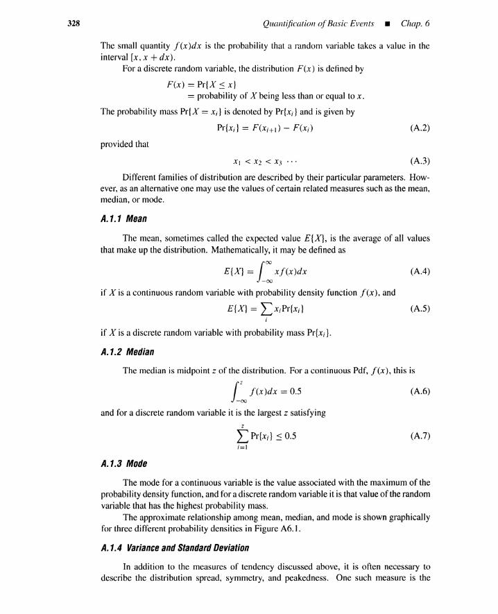
(A.2)
328 Quantification of Basic Events _ Chap. 6
The small quantity f t» )dx is the probability that a random variable takes a value in theinterval [x, x +dx).
For a discrete random variable, the distribution F(x) is defined by
F(x) == PrIX ~ x}== probability of X being less than or equal to x.
The probability mass PrIX == x;} is denoted by Pr{x;} and is given by
Pr{x;} == F(X;+I) - F(x;)
provided that
Xl < X2 < X3 ... (A.3)
Different families of distribution are described by their particular parameters. How-ever, as an alternative one may use the values of certain related measures such as the mean,median, or mode.
A.1.1 Mean
The mean, sometimes called the expected value E{X}, is the average of all valuesthat make up the distribution. Mathematically, it may be defined as
E{X} =i: xf(x)dx (AA)
if X is a continuous random variable with probability density function f tx), and
E{X} == Lx;Pr{x;} (A.5)
if X is a discrete random variable with probability mass Prlx»].
A.1.2 Median
The median is midpoint z of the distribution. For a continuous Pdf, [tx), this is
i~ f(x )dx = 0.5
and for a discrete random variable it is the largest z satisfyingz
L Pr{x;} ~ 0.5;=1
A.1.3 Mode
(A.6)
(A.7)
The mode for a continuous variable is the value associated with the maximum of theprobability density function, and for a discrete random variable it is that valueof the randomvariable that has the highest probability mass.
The approximate relationship among mean, median, and mode is shown graphicallyfor three different probability densities in Figure A6.1.
A.1.4 Variance and Standard Deviation
In addition to the measures of tendency discussed above, it is often necessary todescribe the distribution spread, symmetry, and peakedness. One such measure is the
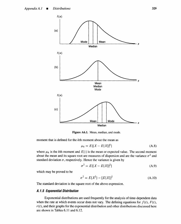
Appendix A.l • Distributions 329
f(x)
Mode Mean
Median
(a)
f(x)
(b)
~~-------_..I--_--------x
MeanMedianMode
f(x)
(c)
Mean
Median
Figure A6.1. Mean, median, and mode.
moment that is defined for the kth moment about the mean as
(A.8)
where J1;k is the kth moment and E{.} is the mean or expected value. The second momentabout the mean and its square root are measures of dispersion and are the variance a 2 andstandard deviation a, respectively. Hence the variance is given by
(A.9)
which may be proved to be
(A.IO)
The standard deviation is the square root of the above expression.
A.1.5 Exponential Distribution
Exponential distributions are used frequently for the analysis of time-dependent datawhen the rate at which events occur does not vary. The defining equations for f(t), F(t),r(t), and their graphs for the exponential distribution and other distributions discussed hereare shown in Tables 6.11 and 6.12.

330 Quantification ofBasic Events _ Chap. 6
A.1.6 Normal Distribution
The normal (or Gaussian) distribution is the best-known two-parameter distribution.All normal distributions are symmetric, and the two distribution parameters, /1 and a, areits mean and standard deviation.
Normal distributions are frequently used to describe equipment that has increasingfailure rates with time. The equations and graphs for j'(t), F(t), and ret) for a normaldistribution are shown in Tables 6.11 and 6.12. The mean time to failure, /1, is obtained bysimple averaging and is frequently called the first moment. The sample average Ji is calleda sample mean.
n- -1~/1 == n ~ t;
;=1(A.II)
where t; is the time to failure for sample t, and n is the total number of samples.The estimation of variance a 2 or standard deviation a depends on whether mean /1
is known or unknown. For a known mean /1, variance estimator a 2 is given by11
a 2 == n- I L(t; - /1)2
;=1(A.12)
For unknownmean /1, the sample meanJi is used in place of /1, and sample size n is replacedby n - 1.
n
a 2 == (n - 1)-1 L(t; _ji)2;=1
(A.13)
This sample variance is frequently denoted by S2. It can be proven that random variablesIi and S2 are mutually independent.
Normal distribution F(t) is difficult to evaluate; however, there are tabulations ofintegrals in statistics and/or reliability texts. Special graph paper, which can be used totransform an S-shaped F(t) curve to a straight line function, is available.
A.1.7 Log-Normal Distribution
A log-normal distribution is similar to a normal distribution with the exception thatthe logarithm of the values of random variables, rather than the values themselves, areassumed to be normally distributed. Thus all values are positive, the distribution is skewedto the right, and the skewness is a function of a. The availability of log-normal probabilitypaper makes it relatively easy to test experimental data to see whether they are distributedlog-normally.
Log-normal distributions are encountered frequently in metal-fatigue testing, main-tainability data (time to repair), and chemical-process equipment failures and repairs. Thisdistribution is used for uncertainty propagation in Chapter II.
A.1.8 Weibull Distribution
Among all the distributions available for reliability calculations, the Weibull distri-bution is the only one unique to the field. In his original paper, "A distribution of wideapplicability," Professor Weibull [5], who was studying metallurgical failures, argued thatnormal distributions require that initial metallurgical strengths be normally distributed andthat what was needed was a function that could embrace a great variety of distributions(including the normal).
Appendix A.l • Distributions 331
The Weibull distribution is a three-parameter (y, a, fJ) distribution (unlike the normal,which has only two), where:
y = the time until F(/) = 0, and is a datum parameter; that is, failures start occurring attime 1
a = the characteristic life, and is a scale parameterfJ = a shape parameter
As can be seen from Table 6.12, the Weibull distribution assumes a great variety ofshapes. If y = 0, that is, failures start occurring at time zero, or if the time axis is shiftedto conform to this requirement, then we see that
1. for fJ < 1, we have a decreasing failure rate (such as may exist at the beginningof a bathtub curve);
2. for fJ = 1, r(/) == A = fJ/a = Y]«, and we have an exponential reliability curve;
3. for 1 < fJ < 2 (not shown), we have a skewed normal distribution (failure rateincreases at a decreasing rate as t increases);
4. for fJ > 2, the curve approaches a normal distribution.
The gamma function I' (.) for the Weibull mean and variance in Table 6.11 is a gen-eralization of a factorial [f (x + 1) = x! for integer x], and is defined by
rex) = 100
tX-1e-tdt (A.14)
By suitable arrangement of the variables, a can be obtained by reading the value of(I - y) at F(/) = 0.63. Methods for obtaining y, which must frequently be guessed, havebeen published [2].
A.1.9 Binomial Distribution
Denote by P the probability of failure for a component. Assume N identical compo-nents are tested. Then the number of failures Y is a random variable with probability
N!Pr{y = n} = p n(1 - p)N-n (A.I5)
n!(N - n)!
The binomial distribution has mean N P and variance N P(1 - P).A generalization of this distribution is a multinomial distribution. Suppose that type
i event occurs with probability Pi. Assume k types of events and that a total of m trials areperformed. Denote by Yi the total number of type i events observed. Then, random vector(Yl, ... , Yk) follows a multinomial distribution
{ m! Yl YkPrYl,···,Yk}= PI ··.PkYl!··· Yk!
A.1.10 Poisson Distribution
(A.I6)
Consider a component that fails according to an exponential distribution. Assumethat the failed component can be repaired instantaneously, that is, a renewal process. Thenumber of failures n to time 1 is a random variable with a Poisson distribution probability(Tables 6.11 and 6.12).
n = 0,1, ... (A. I?)

(A.18)
(A.19)
332 Quantification ofBasic Events - Chap. 6
The Poisson distribution is an approximationto the binomialdistributionfunction fora large number of samples N, and small failure probability P with a constraint N P == At.
N! (At)ne-At
Pr{y == n} == pn(1 _ p)n :::: ---n!(N-n)! n!
Equation (A.18) is called a Poisson approximation.The Poisson distribution is used to calculate the probability of a certain number of
events occurring in a large system, given a constant failure rate Aand a time t.One would use the F(n) in Table 6.11 that is, the probability of having n or less
failures in time t. In an expansion for F(n),
(At)2 (At)nF(n) == e-Af + ue:" + __«:" + ... + __«"
2 n!
the first term defines the probability of no component failures, the second term defines theprobability of one component failure, and so forth.
A.1.11 Gamma Distribution
The gamma distribution probability density is (Table6.11)
I (t )13- 1-fir]
f/r(t3) ~ e , 13 > 0, f/ > 0 (A.20)
Assume an instantaneouslyrepairable component that fails according to an exponen-tial distribution with failure rate I/Yl. Consider for integer f3 an event that the componentfails f3 or more times. This event is equivalent to the occurrence of f3 or more shocks withrate I/Yl. Then thedensity j'(t) for such aneventat time t is givenby the gammadistributionwith integer fJ
. e-At (At)fJ- 1
j(t) = (13 _ I)! A (A.21)
This is called an Erlang probability density. The gammadensity of (A.20) is a mathematicalgeneralization of (A.21) because
A.1.12 Other Distributions
r(fJ) == (fJ - I)!, fJ: integer (A.22)
Tables6.11 and 6.12 include Gumbel, inverseGaussian, and beta distributions.
A.2 ACONSTANT-FAllURE-RATE PROPERTY
We first prove equation (6.52). The failure during [t, t +dt) occurs in a repair-to-failureprocess. Let s be a survival age of the component that is normal at time t. In other words,assume that the component has been normal since time t - s and is normal at time t. Thebridge rule of equation (A.29), appendix of Chapter 3, can be written in integral form as
Pr{AjC} =f Pr{Als, c}p{slC}ds (A.23)

Appendix A.4 • Distributions 333
where p{sIC} is the conditional probability density of s, given that event C occurs. Theterm p{sIC}ds is the probability of "bridge [s, s+ds)," and the term Pr{Als, C} is the prob-ability of the occurrence of event A when we have passed through the bridge. The integralin (A.23) is the representation of Pr{A IC} by the sum of all possible bridges. Define thefollowing events and parameter s.
A = Failure during [t, t + dt)s = The normal component has survival age s at time t
C = The component was as good as new at time zero and is normal at time t
Because the component failure characteristics at time t are assumed to depend onlyon the survival age s at time t, we have
Pr{Als, C} = Pr{Als} = r(s)dt
From the definition of A(t), we obtain
Pr{AIC} = A(t)dt
Substituting equations (A.24) and (A.25) into equation (A.23), we have
A(t)dt = dt ·f r(s)p{sIClds
For the constant-failure rate r,
A(t)dt = dt . r · f p{slClds = dt . r · 1
yielding equation (6.52).
A.3 DERIVATION OF UNAVAILABILITY FORMULA
(A.24)
(A.25)
(A.26)
(A.27)
We now prove equation (6.96). Denote by E {.} the operation of taking the expected value.In general,
E{x(t)} = E{XO,I(t)} - E{XI,O(t)}
holds. The expected value E{x(t)} of x(t) is
E{x(t)} = 1 x Pr{x(t) = I} + 0 x Pr{x(t) = O}= Pr{x(t) = I}
yielding
E{x(t)} = Q(t)
(A.28)
(A.29)
(A.30)
Because XOI (t) is the number of failures to time t, E{XO,l (t)} is the expected number offailures to that time.
E{XO,l(t)} = W(O,t)
Similarly,
E{Xl,O(t)} = V(O, t)
Equations (A.28), (A.30), (A.31), and (A.32) yield (6.96).
(A.31)
(A.32)

334 Quantification ofBasic Events - Chap. 6
A.4 COMPUTATIONAL PROCEDURE FOR INCOMPLETE TEST DATA
Suppose that N items fail, in turn, at discrete lives tl, t2, ... , tm . Denote by r, the numberof failures at lifetime t;. The probability of failure at lifetime tl can be approximated byP(tl) = rl / N, at lifetime t: by P(t2) = r2/N, and, in general, by P(t;) = r, / N.
The above approximation is applicable when all the items concerned continue to fail.In many cases, however, some items are taken out of use for reasons other than failures,hence affecting the numbersexposed to failuresat different lifetimes. Therefore a correctionto take this into account must be included in the calculation.
Suppose that N items have been put into use and failure occurs at discrete livestl, ti. t3, ... , the number of failures occurring at each lifetime are rl, r2, rs- ... , and thenumber of items actually exposed to failure at each lifetime are N I , N2, N3, ••••
Because rl failedat tl, theoriginal numberhas been reducedto N I -rl. The proportionactually failing at t: is r2/ N2, so the number that would have failed, had N I proceeded tofailure, is
r:(NI - rl)- (A.33)
N2
and the proportion of N I expected to fail at t: is
r:P(t2) = (NI - rl)-- (A.34)
N IN2
We now proceed in the same manner to estimate the proportion of NI that would fail at t3.
If the original number had been allowed to proceed to failure, the number exposed tofailure at t3 would be
N, - [rl + (NI - rd ~2]
and the proportion of N I expected to fail at t3 is
P(t3) = {NI - [r l + (NI - r l )!2- ] }~N2 N 1N3
The same process can be repeated for subsequent values.
A.5 MEDIAN-RANK PLOTTING POSITION
(A.35)
(A.36)
Suppose that n times to failure are arranged in increasing order: tl, ... , t;, ... , tn' Abscissavalues for plotting points are obtained from these times to failures. We also need the cor-responding estimate P; of the cumulative distribution function F(t). A primitive estimatori / n is unsuitable because it indicates that 100% of the population would fail prior to thelargest time to failure Is for the sample size n = 5.
For an unknown distribution function F(t), define P; by P; = F(t;). This P; isa random variable because t, varies from sample to sample. It can be shown that theprobability density function g(P;) of P; is given by [4]
n' . I .( ~. ) _ . pl- (1 _ ~.)"-1
g 1 - (i _ 1) !(n _ i)! ; 1
In other words, random variable P; follows a beta distribution.
(A.37)

Chap. 6 • Problems
The median Pi value of this beta distribution is its median rank.
1Ag(P;)dP; = 0.5
These values can be obtained from tables of incomplete beta functions.
s.c«. n) =1x
1"-1(1 - y)n-1dy
An approximation to the median-rank value is given by
A i - 0.311 == ---
n +0.4
A simpler form is
A i - 0.5Pi == - -
n
A.6 FAILURE AND REPAIR BASIC DEFINITIONS
Table A6.1 provides a summary of basic failure and repair definitions.
PROBLEMS
335
(A.38)
(A.39)
(A.40)
(A.41)
6.1. Calculate, using the mortality data of Table 6.1, the reliability R(t), failure density .I'(t),
and failure rate r(t) for:(a) a man living to be 60 years old (t = 0 means zero years);(b) a man living to be 15 years and I day after his 60th birthday (t = 0 means 60 years).
6.2. Calculate values for R(t), F(t), r(t), A(t), Q(t), w(t), W(O, t), and A(t) for the tencomponents of Figure 6.7 at 3 hr and 8 hr.
6.3. Prove MTTF equation (6.32).
6.4. Using the values shown in Figure 6.7, calculate G(t), g(t), m(t), and MITR.
6.5. Use the data of Figure 6.7 to obtain JL(t) and v(t) at t = 3 and also V (0, t).
6.6. Obtain f tt), r(t), g(t), and m(t), assuming
8 1F(t) = 1 - =je- t + =je-St
, G (t) = I - «"
6.7. Suppose that
1j'(t) = "2 (e- t + 3e- 3t) , g(t) = 1.5e-1.5t
(a) Show that the following w(t) and v(t) satisfy the (6.89) equations.
1 3w(t) = 4 (3 + 5e- 4t) , v(t) = 4 (1 - e-4t
)
(b) Obtain W (0, t), V (0, t), Q(t), A(t), and JL(t).
(c) Obtain r(t) to confirm (6.109).
6.8. A device has a constant failure rate of A = 10- 5 failures per hour.(a) What is its reliability for an operating period of 1000 hr?(b) If there are 1000 such devices, how many will fail in 1000 hr?(c) What is the reliability for an operating time equal to the MITF?
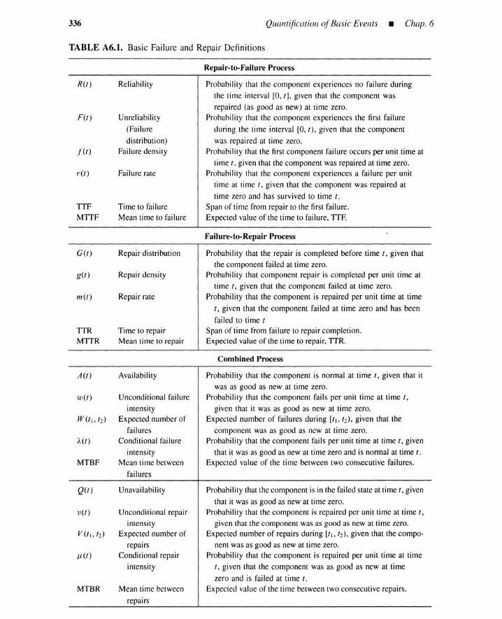
336
TABLE A6.1. Basic Failure and Repair Definitions
Quantification o.fBasic Events - Chap. 6
R(t) Reliability
F(t) Unreliability(Failuredistribution)
.l(t) Failure density
r(/) Failure rate
TTF Time to failureMTIF Mean time to failure
G(t) Repair distribution
g(t) Repair density
111 (t) Repair rate
TTR Time to repairMTTR Mean time to repair
A(t) Availability
w(l) Unconditional failureintensity
W(tI,12) Expected number offailures
A(t) Conditional failureintensity
MTBF Mean time betweenfailures
Q(t) Unavailability
v(l) Unconditional repairintensity
V (11, (2) Expected number ofrepairs
J-l(t) Conditional repairintensity
MTBR Mean time betweenrepairs
Repair-to-Failure Process
Probability that the component experiences no failure duringthe time interval [0, I], given that the component wasrepaired (as good as new) at time zero.
Probability that the component experiences the first failureduring the time interval [0, I), given that the componentwas repaired at time zero.
Probability that the first component failure occurs per unit time attime I, given that the component was repaired at time zero.
Probability that the component experiences a failure per unittime at time I, given that the component was repaired attime zero and has survived to time I.
Span of time from repair to the first failure.Expected value of the time to failure, TIF.
Failure-to-Repair Process
Probability that the repair is completed before time I, given thatthe component failed at time zero.
Probability that component repair is completed per unit time attime I, given that the component failed at time zero.
Probability that the component is repaired per unit time at timeI, given that the component failed at time zero and has beenfailed to time I
Span of time from failure to repair completion.Expected value of the time to repair, TIR.
Combined Process
Probability that the component is normal at time I, given that itwas as good as new at time zero.
Probability that the component fails per unit time at time I,
given that it was as good as new at time zero.Expected number of failures during [11, (2), given that the
component was as good as new at time zero.Probability that the component fails per unit time at time I, given
that it was as good as new at time zero and is normal at time I.
Expected value of the time between two consecutive failures.
Probability that the component is in the failed state at time I, giventhat it was as good as new at time zero.
Probability that the component is repaired per unit time at time I,
given that the component was as good as new at time zero.Expected number of repairs during [11, (2), given that the compo-
nent was as good as new at time zero.Probability that the component is repaired per unit time at time
I, given that the component was as good as new at timezero and is failed at time I.
Expected value of the time between two consecutive repairs.
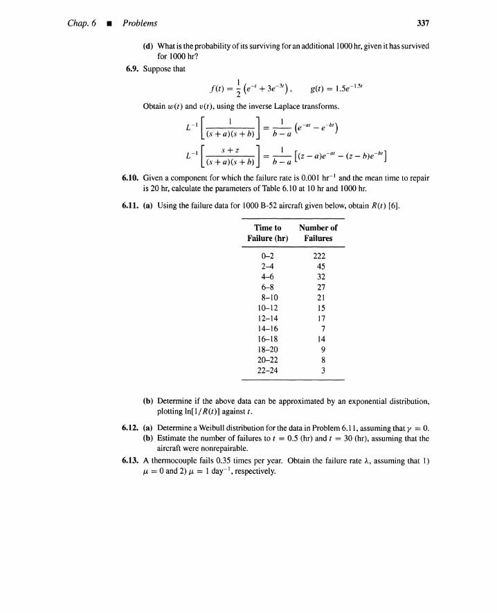
Chap. 6 • Problems 337
(d) What is the probability of its surviving for an additional 1000 hr, given it has survivedfor 1000 hr?
6.9. Suppose that
g(t) = 1.5e-1.5t
Obtain w(t) and v(t), using the inverse Laplace transforms.
L-1 [ I ] 1 (-at -ht(s + a)(s + b) = b _ a e - e )
L -1 [ S + z ] = _1_ [(z _ase" _ (z _ b)e-bt ]
(s+a)(s+b) b-a
6.10. Given a component for which the failure rate is 0.001 hr" and the mean time to repairis 20 hr, calculate the parameters of Table 6. 10 at 10 hr and 1000 hr.
6.11. (a) Using the failure data for 1000 8-52 aircraft given below, obtain R(t) [6].
Time toFailure (hr)
0-22-44-66-88-10
10-1212-1414-1616-18
18-2020-2222-24
Number ofFailures
2224532
272115177
14983
(b) Determine if the above data can be approximated by an exponential distribution,plotting In[l/R(t)] against t.
6.12. (a) Determine a Weibull distribution for the data in Problem 6.11, assuming that y = O.(b) Estimate the number of failures to t = 0.5 (hr) and t = 30 (hr), assuming that the
aircraft were nonrepairable.
6.13. A thermocouple fails 0.35 times per year. Obtain the failure rate A, assuming that 1)
Jvt = 0 and 2) Jvt = 1 day", respectively.
7onfidence Intervals
7.1 CLASSICAL CONFIDENCE LIMITS
7.1.1 Introduction
When the statistical distribution of a failure or repair characteristic (time to failureor time to repair) of a population is known, the probability of a population member'shaving a particular characteristic can be calculated. On the other hand, as mentioned in thepreceding chapter, measurement of the characteristic of every member in a population isseldom possible because such a determination would be too time-consuming and expensive,particularly if the measurement destroys the member. Thus methods for estimating thecharacteristics of a population from sample data are required.
It is difficult to generalize about a given population when we measure only the char-acteristic of a sample because that sample may not be representative of the population. Asthe sample size increases, the sample parameters and those of the population will, of course,agree more closely.
Although we cannot be certain that a sample is representative of a population, it isusually possible to associate a degree of assurance with a sample characteristic. That degreeof assurance is called confidence, and can be defined as the level of certainty associatedwith a conclusion based on the results of sampling.
To illustrate the above statements, suppose that a set of ten identical components arelife-tested for a specified length of time. At the end of the test, there are five survivors. Basedon these experiments, we would expect that the components have an average reliability of0.5 for the test time span. However, that is far from certain. We would not be surprised ifthe true reliability was 0.4, but we would deem it unlikely that the reliability was 0.01 or0.99.
339
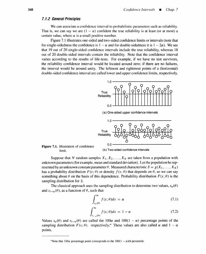
340 Confidence Intervals _ Chap. 7
7.1.2 General Principles
We can associate a confidence interval to probabilistic parameters such as reliability.That is, we can say we are (I - a) confident the true reliability is at least (or at most) acertain value, where a is a small positive number.
Figure 7.1 illustrates one-sided and two-sided confidence limits or intervals (note thatfor single-sidedness the confidence is I - a and for double-sidedness it is 1 - 2a). We seethat 19 out of 20 single-sided confidence intervals include the true reliability, whereas 18out of 20 double-sided intervals contain the reliability. Note that the confidence intervalvaries according to the results of life-tests. For example, if we have no test survivors,the reliability confidence interval would be located around zero; if there are no failures,the interval would be around unity. The leftmost and rightmost points of a (horizontal)double-sided confidence interval are called lower and upper confidence limits, respectively.
1.0 --------------
TrueReliability
(a) One-sided upper confidence intervals
1.0--------------
TrueReliability
Figure 7.1. Illustration of confidencelimit.
0.0 --------------
(b) Two-sided confidence intervals
Suppose that N random samples XI, X2, ... , XN are taken from a population withunknownparameters (forexample, meanand standarddeviation). Let the population be rep-resented byan unknownconstant parameter0 . Measuredcharacteristic S == g(X I, ... , XN)has a probability distribution F(s; 0) or density fts; 0) that depends on 0, so we can saysomething about 0 on the basis of this dependence. Probability distribution F (s; e) is thesampling distribution for S.
The classical approach uses the sampling distribution to determine two values, sa(e)and SI-ace), as a function of 0, such that
100 fts; (})ds = ex (7.1)su(O)
100 [ts: (})ds = I - ex (7.2)SI-u(O)
Values sa(O) and SI-a(O) are called the 100a and 100(1 - a) percentage points of thesampling distribution Fts; e). respectively;" These values are also called a and 1 - apoints.
*Note that 100a percentage point corresponds to the 100(1 - a )th percentile.
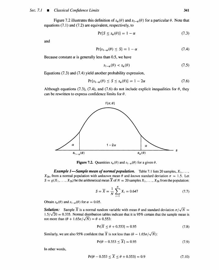
Sec. 7.1 • Classical Confidence Limits 341
Figure 7.2 illustrates this definition of sa(O) and sl-a(lJ) for a particular o. Note thatequations (7.1) and (7.2) are equivalent, respectively, to
Pr{S ~ sa(O)} = 1 - a
and
Because constant a is generally less than 0.5, we have
Sl-a(O) < sa(O)
Equations (7.3) and (7.4) yield another probability expression,
Pr{sl-a(O) ~ S ~ sa(O)} = 1 - 2a
(7.3)
(7.4)
(7.5)
(7.6)
Although equations (7.3), (7.4), and (7.6) do not include explicit inequalities for 0, theycan be rewritten to express confidence limits for o.
tis; 8)
5
(7.7)
Figure 7.2. Quantities sa«(}) and Sl-a«(}) for a given ().
Example I-Sample mean ofnormal population. Table 7.1 lists 20 samples, Xl, ... ,X20 , from a normal population with unknown mean () and known standard deviation a = 1.5. LetS = g(X1, .•. , X20) be the arithmetical mean Xof N = 20 samples Xl, ... , X20 from the population:
1 N
S = X= N L Xi = 0.647;=1
Obtain sa«(}) and Sl-a«(}) for ex = 0.05.
Solution: Sample X is a normal random variable with mean () and standard deviation a /,IN =1.5/ J20 = 0.335. Normal distribution tables indicate that it is 95% certain that the sample mean isnot more than «() + 1.65a /,IN) = () + 0.553:
PrIX ~ () + 0.553} = 0.95
Similarly, we are also 95% confident that Xis not less than «() - 1.65a/ ,IN):
Pr{(} - 0.553 ~ X} = 0.95
In other words,
Pr{(} - 0.553 :s X :s () + 0.553} = 0.9
(7.8)
(7.9)
(7.10)

342 Confidence Intervals _ Chap. 7
TABLE 7.1. Twenty Samples from aNormal Population (():unknown, a == 1.5)
Thus SI-aCO) and saCO) are given by
0.090-0.105
2.280-0.051
0.182-1.610
1.100-1.200
1.1300.405
0.0490.588
-0.6935.3101.2801.7900.4050.916
-1.2002.280
'\'l-aCO) = 0 - 0.553
Sa (0) = 0 + 0.553
(7.11)
(7.12)
•Assume that SI-a (.) and Sa (.) are the monotonically increasing functions of () shown
in Figure 7.3 (similar representations are possible for monotonically decreasing cases ormore general cases). Consider now rewriting equations (7.3), (7.4), and (7.6) in a formsuitable for expressing confidence intervals. Equation (7.3) shows that the random variableS == g(X I , ••. , X N ) is not more than sa(()) with probability (1 - ex) when we repeat alarge number of experiments, each of which yields possibly different sets of N observationsX I, ... , XNand S. We now define a new random variable Sa related to S, such that
(7.13)
where S is the observed characteristic and Sa (.) the known function of (). Or equivalently,
(7.14)
Variable Sa is illustrated in Figure 7.3. The inequality S < sa(') describes the factthat variable Sa, thus defined, falls on the left-hand side of constant ():
Hence from equation (7.3),
Pr{Sa:::: ()} == 1 - ex
(7.15)
(7.16)
This shows that random variable 8 a determined by S and curve sa(') is a (1 - ex) lowerconfidence limit; variable 8 a == s; I (S) becomes a lower confidence limit for unknownconstant (), with probability (I - ex).
Similarly, we define another random variable 81-a by
(7.17)
where S is the observed characteristic and S I-a (.) is the known function of(); or, equivalently,
(7.18)

Sec. 7.1 • Classical Confidence Limits 343
ooa
s
Sa (0) f---- - --- ------ - =-'--
Figure 7.3. Variable 8 determined from S and curves saO and SI -aO.
Random variable e l - a is illustrated in Figure 7.3. Equation (7.4) yields
Pr{O :s e l - a } = I - a (7.19)
Thus variable el-a gives an upper confidence limit for constant O.Combining equations (7.16) and (7.19), we have
Pr{ea :s 0 :s e l - a } = I - 2a (7.20)
Random interval [ea. e l - a] becomes the 100(1 - 2a) % confidence interval. In otherwords, the interval includes true parameter 0 with probability I - 2a. Note that inequalitiesare reversed for confidence limits and percentage points.
Sl-a < Sa (7.21)
For monotonically decreasing sa(O) and SI-a(O), the confidence interval is [e l - a • ea ] :
Increasing .I'ex. .1'1 _ a Decreasing .I'ex.SI -a
Interval
Example 2-Conjidence interval of population mean. Obtain the 95% single-sided upper and lower limits and the 90% double-sided interval for the population mean () in Ex-ample I.
Solution: Equations (7. I I) and (7.12) and the definition of 8 1- a and 8 a [see equations (7.13) and(7.17)] yield
8 1- a - 0.553 = X=} 8 1- a = X + 0.553 = 0.647 + 0.553 = 1.20 (7.22)
8 a + 0.553 = X=} 8 a = X - 0.553 = 0.647 - 0.553 = 0.094 (7.23)

344 Confidence Intervals _ Chap. 7
Variable(-)l-a and (-)a are the 95% upper and lower single-sided confidence limits, respectively. Thedouble-sided confidence interval is
[(-)a, (-)I-a] = [0.094, 1.20]
Equation (7.10) can be rewritten as
Pr{X - 0.553 :s () :s X +0.553} == 0.90
(7.24)
•(7.25)
(7.26)
Although () is an unknown constant in the classical approach, this expression is correctbecause X is a random variable. This shows that random interval [X - 0.553, X + 0.553]contains the unknown constant with probability 0.9. When sample value 0.647 is substitutedfor X, the expression is not correct any more because there is no random variable, that is,
Pr{0.647 - 0.553 :s () :s 0.647 + 0.553} == Pr{0.094 :s () :s 1.20}
== 0.90, (incorrect)
This expression is, however, convenient for confidence interval manipulations.
Example 3-Normal population with unknown variance. Assume that the N = 20samples in Example 1 are drawn from a normal population with unknown mean 0 and unknownstandard deviation a. Obtain the 90% confidence interval for the mean O.
Solution: Sample meanXand sample standard deviation0 are given by (Section A.I.6, Appendixof Chapter 6)
_ 1 N
X = N LX; =0.647;=1
1 N
(j = N _ I E(X; - X)2 = 1.54;=1
(7.27)
(7.28)
It is well known that the following variable t follows a Student's t distribution* with N - I degreesof freedom (see Case 3, Student's t column of Table A.2 in Appendix A.l to this chapter; note thatsample variance0 2 is denoted by S2 in this table).
t == v1V (X - O)/a 'V stu*(N - I) = stu*(19) (7.29)
Denote by ta .19 and tl-a.19 the ex and 1 - ex points of the Student's distribution, that is,
Pr{ta .19 ~ t} = ex = 0.05
Pr{tl-a .19 ~ t} = 1 - ex = 0.95
Then
Pr{tl-a .19 ~ v1V(X - O)/a ~ ta .19 } = 1 - 2ex
or, in terms of the sampling distribution percentage points of X,Pr{sl-a(O) ::s X ::s Sa(O)} = 1 - 2ex
where
(7.30)
(7.31)
(7.32)
atl-a.19SI-a(O) == (1+ v1V ' (7.33)
*These properties were first investigated by W. S. Gosset, who was one of the first industrial statisticians.He worked as a chemist for the Guinness Brewing Company. Because Guinness would not allow him to publishhis work, it appeared under the pen name "Student/'[J]

Sec. 7.1 • Classical Confidence Limits 345
Because function sa((}) and Sl-a((}) are monotonically increasing, we have the (1 - 2a) confidenceinterval
- atl-a,198 1- a == X - ,IN (7.34)
Equation (7.31) can be rewritten as
Pr {x- ta,19a< () < X - t 1- a,19a } = 1 - 2a,IN- -,IN , (7.35)
yielding the same confidence interval as equation (7.34).From a Student's t table we have ta,19 = 1.729. The Student's t distribution is symmetric
around t = 0, and we have tl-a,19 = -1.729. From sample values of X and a, we have a 90%confidence interval for mean () under an unknown standard deviation.
[0.052, 1.2] (7.36)
Notice that this interval is wider than that of Example 2 where the true standard deviation a isknown. •
Example 4-Student's t approximation by a normal distribution. For large degreesof freedom v, say v ::: 30, the Student's t distribution can be approximated by a normal distributionwith mean zero and variance unity. Repeat Example 3 for this approximation.
Solution: From normal distribution tables, we have ta,19 = -tl-a.19 = 1.65, yielding the 90%confidence interval for mean ()
() E [0.079, 1.22] (7.37)
Although the degrees of freedom, v = 19, is smaller than 30, this interval gives an approximation ofthe interval calculated in Example 3. •
Example 5-Hypothesis test ofequal means. Consider the 20 samples of Example 1.Assume that the first ten samples come from a normal population with mean (}1 and standard deviation01, while the remaining ten samples come from a second normal population with mean (}2 and standarddeviation 02. Evaluate the hypothesis that the two mean values are equal, that is,
(7.38)
Solution: From the two sets of samples, sample means (X 1 and X2) and sample standard deviationseat and 02) are calculated as follows.
Xl = 0.222,
01 = 1.13,
X2 = 1.07
02 = 1.83
(7.39)
(7.40)
From Case 2 of the Student's t column of Table A.2, Appendix A.l, we observe that, under hypothesisH, random variable
(7.41)
has a Student's t distribution with n1 + n: - 2 degrees of freedom. Therefore, we are 90% confidentthat variable t lies in interval [tl-a,lS, ta.18], a = 0.05. From a Student's t distribution table, to.05.18 =1.734 = -to.95.18' Thus
Pr{-1.734 ~ t ~ 1.734} = 0.90 (7.42)

(7.44)
346 Confidence Intervals • Chap. 7
On the other hand, a sample value of t is calculated as
0.222 - 1.07t = I = -1.25 (7.43)
[(10 - 1)(1.13)2 + (10 - 1)(1.83)2]2 I
10+ 10 _ 2 [(1/10) + (1/10)]2
This value lies in the 90% interval of equation (7.42), and the hypothesis cannot be rejected; if a tvalue is not included in the interval, the hypothesis is rejected because the observed t value is toolarge or too small in view of the hypothesis. •
Example 6-Hypothesis test of equal variances. For two normal populations, equalvariance hypothesis can be tested by an F distribution. From the Case 2 row of the F distri-bution column of Table A.3, Appendix A.I, we see that a ratio of two sample variances followan F distribution. An equal variance hypothesis can be evaluated similarly to the equal meanhypothesis. •
Example 7-Variance confidence interval. Obtain the 90% confidence interval forunknown variancea 2 in Example 3.
Solution: As shownin Case 2 of the X2 distributioncolumn of TableA7.1, AppendixA.l, randomvariable (N - I )a2/a 2 is X2 distributed with N - 1degrees of freedom, that is,
(N - l)a2
--- rv csq*(n - 1) = csq*(19)
or
19 X 1.542
---- = 45.I/a 2rv csq2(19) (7.45)
Let X(;.05.19 and X(;.95.19 be the 5 and 95 percentage points of the chi-square distribution, respectively.Then from standard chi-square tables X(;.05.19 = 30.14 and Xl95.19 = 10.12. Thus
or, equivalently,
Pr{IO.12 ~ 45.1/a 2 ~ 30.14} = 0.9
Pr{I. 22 :::: a :::: 2. I I} = 0.9
(7.46)
(7.47)
Again, expressions (7.45), (7.46), and (7.47) are used only for convenience because they involve norandom variables. This interval includes the true standard variation,a = 1.5 of Example 1. •
7.1.3 Types 01 Lile-Tests
Suppose N identicalcomponents are placed on life-testsand no components are takenout for service before test termination. The two test options are [2]:
1. Time-terminated test. Life-test is terminated at time T before all N componentshave failed.
2. Failure-terminated test. Test is terminated at the time of the rth, r ~ N failure.
In time-terminated tests, T is fixed, and the number of failures r and all the failuretimes tl ~ t: ~ ... ~ t,. sTare random variables. In failure-terminated tests, the numberof failures r is fixed, and the r failure times and T == tr are random variables.
7.1.4 Confidence Limits forMean Time to Failure
Assume failure-terminated test for N components, with an exponential time-to-fail-ure distribution for each component. A point estimate e for the true mean time to
Sec. 7.1 • Classical Confidence Limits
failure 8 = 1IA, is
A (N - r)tr + L:;=l t;8 = -------
r
= S, the observed characteristic
347
(7.48)
(7.49)
(7.50)
This estimate is called the maximum-likelihood estimator for MTTF. It can be shown that2r SI8 follows a chi-square distribution with 2r degrees of freedom [2,3] (see the lastexpression in Case 3 of the X2 distribution column of Table A7.1, Appendix A.l). Let X;,2r
and Xr-cx,2r be the 100a and 100(1 - a) percentage points of the chi-square distributionobtained from standard chi-square tables [2-5]. From the definition of percentage points,
{2 2r S } { 2 2r S}
Pr Xcx,2r S T = a, Pr XI-cx,2r S T = 1 - a
These two expressions can be rewritten as
(7.51)
(7.52)
yielding
2rS 2rS8 cx == x~(2r)' 8 1- cx == 2
~ XI_cx (2r )
Quantities 8 cx and 8 1- cx give 100(1 - a)% the lower and upper confidence limits, whereasthe range [8 cx , 8 1- cx ] becomes the 100(1 - 2a)% confidence interval.
Example 8-MTTF ofexponential distribution. Assume 30 identical components areplaced on failure-terminated test with r = 20. The 20th failure has a time to failure of 39.89 min.,that is, T = 39.89, and the other 19 times to failure are listed in Table 7.2, along with times to failurethat would occur if the test were to continue after the 20th failure, assuming the failures follow anexponential distribution. Find the 95% two-sided confidence interval for the MTTF.
Solution: N = 30, r = 20, T = 39.89, ex = 0.025.
{) = s = (30 - 20) x 39.89 + 291.09 = 34.520
From the chi-square table in reference [3]:
X;.2r = X5.025.40 = 59.34
X;-a.2r = X5.975.40 = 24.43
Equation (7.52) yields
34.5Sa = 2 x 30 X -- = 23.3
59.34
34.58 1- a = 2 X 30 X -- = 56.5
24.43
Then
23.3 ::: fJ ::: 56.5
(7.53)
(7.54)
(7.55)
(7.56)
(7.57)
(7.58)
that is, we are 95% confident that the mean time to failure (fJ) is in the interval [23.3, 56.5]. As a matterof fact, TTFs in Table 7.2 were generated from an exponential distribution with the MTIF = 26.6.The confidence interval includes this true MTTF. •

348 Confidence Intervals _ Chap. 7
TABLE 7.2. TTF Data for Example 8
TTFs up to TTFs after20th Failure 20th Failure
t) 0.26 tIl 11.04 t2] 40.84t: 1.49 t)2 12.07 t22 47.02t3 3.65 t]3 13.61 t23 54.75t4 4.25 t]4 15.07 t24 61.08ts 5.43 tIS 19.28 t2S 64.36t6 6.97 t]6 24.04 t26 64.45
h 8.09 t17 26.16 t27 65.92tx 9.47 tn~ 31.15 t2X 70.82t9 10.18 t)9 38.70 t29 97.32tlO 10.29 t20 39.89 t30 164.26
Example 9-Reliability andfailure rate. The reliabilityofcomponentswithexponentialdistributions was shown to be
(7.59)
Confidence intervals can be obtained by substituting ("')]-0' and (...)0' for 0; hence
(7.60)
Thus for the data in Example 8,
Similarly, the confidence interval for failure rate A is given by
I I--<A<-("'))_0' - - (--)0'
(7.61)
(7.62)
•Example lO-AII components fail. Calculate the 95% confidence interval from the 30
TTFs in Table 7.2 where all 30 components failed.
Solution: Let t), ... .t, be a sequence of n independent and identically distributed exponentialrandom variables. As shown in Case 3 of the X2 column of Table A.I, the quantity (2/0) L:;=] t, ischi-squaredistributed with 2n degrees of freedom, where0 = I/A is a true mean time to failure of theexponential distribution. From a chi-square table, we have X(~.97S.60 = 40.47 and Xl(X)2S.60 = 83.30.Thus
Pr{40.47 ~ (2/0) x 1021.8 ~ 83.30} = 0.9 (7.63)
yielding a slightly narrowerconfidence interval than Example 8 because all 30 TTFs are utilized.
[24.5, 50.5] (7.64)
•Example II-Abnormally long failure times. Consider independentlyand identically
distributed exponential random variablesTTFs denoted by T], ... , T". Suppose that these variableshave not been ordered. Then, as shown in row Case 3 and F distributioncolumn of TableA.3, a ratioof these random variables follows an F distribution. Abnormally long failure times such as T] canbe evaluated by checking whether the F variable is excluded from a confidence interval. In a similar

Sec. 7.J • Classical Confidence Limits 349
way, failure rates for two sets of exponential TTFs can be evaluated. Note that TTFs should not beorderedbecause an increasedorder violates the independence assumption. •
7. 1.5 Confidence Limits for Binomial Distributions
Assume N identical components placed in a time-terminated test with r failures intest period T. We wish to obtain confidence limits for the component reliability R(T) attime T. We begin by replacing static S by discrete random variable r, where
S==r
The S sampling distribution is given by the binomial distribution
N! N (' ,Pr{S == s; R} == R -"[1 - Rr
(N - s)!s!
with R == R(T) corresponding to unknown parameter (3 in Section 7.1.2.Equation (7.3) thus becomes
sa(R) N! .Pr{S :s sa(R)} = L (N _ )' ,RN-"[l - RY 2: 1 - ex
s=o s .s.
(7.65)
(7.66)
(7.67)
Here inequality ~ 1- ex is necessary because S is discrete. The parameter Sa (R) is definedas the smallest satisfying equation (7.67).
A schematic graph of sa(R) is shown in Figure 7.4. Notice that the graph is a mono-tonically decreasing step function in R. We can define Ra for any observed characteristicS, as shown in Figure 7.4, with the exception that Ra is defined as unity when S == 0 isobserved. This Ra corresponds to the Sa in Figure 7.3, where function sa«(3) is monotoni-cally increasing. The event S :::; sa(R) occurs if and only if Ra falls on the right-hand sideof R.
Thus
Pr {R ::s Ra } :::: 1 - ex
(7.68)
(7.69)
and Ra gives 1 - ex, the upper confidence limit for reliability R.Point (Ra , S - 1) is represented by A in Figure 7.4. We notice that, at point A,
inequality (7.67) reduces to an equality for S i= 0 because the value Sa (R) decreases byone. Thus the value of Ra can beobtained for any given S by solving the following equation.
N N'~ . RN - S[l - R ]S == ex for S -I.. 0 (7.70)L.J (N _ )' , a a , -r-s=s s .s.
s; == 1, for S == 0 (7.71)
The above equation can be solved for R by iterative methods, although tables have beencompiled [6]. (See also Problems 7.8 to 7.10.)
Similar to equation (7.70), the lower confidence limit RI-a for R is given by thesolution of the equation
s N'~ . RN
-s[1 - R ]S == ex for S -I.. N (7.72)L.J (N _ )" I-a I-a , -r-s=o s .s.
RI - a == 0, forS == N (7.73)
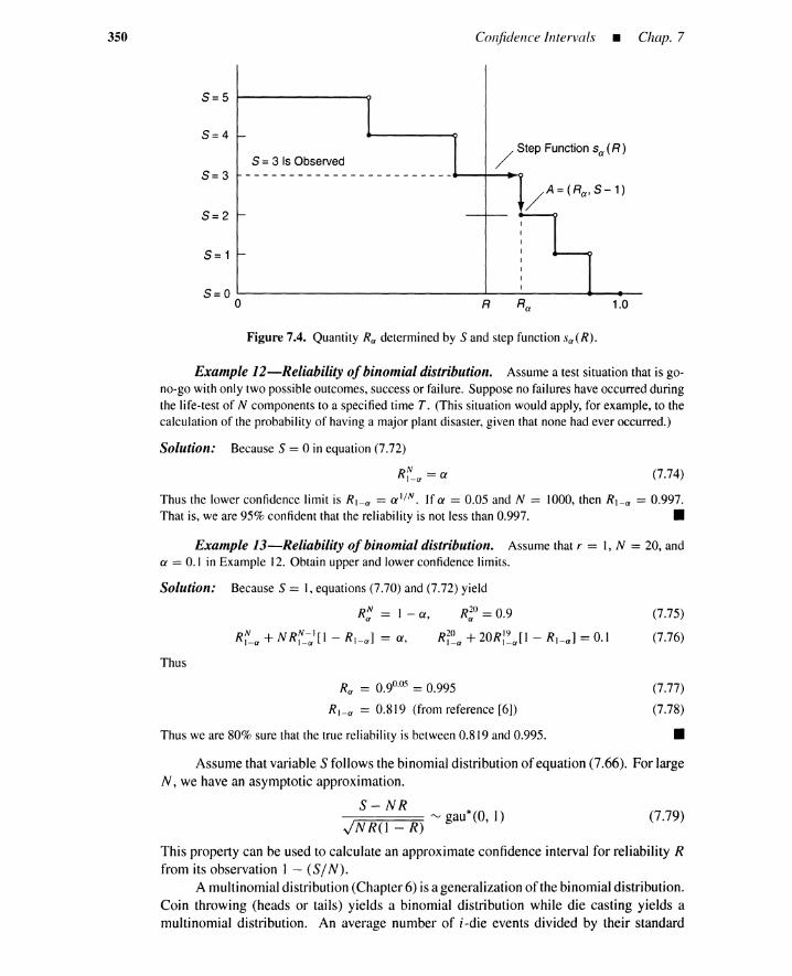
350 Confidence Intervals • Chap. 7
5=5
5=4
------------------------~~--~5=35 =3 Is Observed
/ Step Function sa(R)
5=2
5=1
1.0R5 =0 '------------------'-------...e---.---
o
Figure 7.4. Quantity Ra determined by S and step function Sa (R).
Example 12-Reliability ofbinomial distribution. Assume a test situation that is go-no-go with only two possible outcomes, success or failure. Suppose no failures have occurred duringthe life-test of N components to a specified time T. (This situation would apply, for example, to thecalculation of the probability of having a major plant disaster, given that none had ever occurred.)
Solution: Because S = ain equation (7.72)
R~_a = a (7.74)
Thus the lower confidence limit is R I - a = a'!", If a = 0.05 and N = 1000, then R l - a = 0.997.That is, we are 95% confident that the reliability is not less than 0.997. •
Example 13-Reliability ofbinomial distribution. Assume that r = I, N = 20, anda = 0.1 in Example 12. Obtain upper and lower confidence limits.
Solution: Because S = 1,equations (7.70) and (7.72) yield
R: = 1 - a, R~o = 0.9 (7.75)
R~_a + N R~_~I [1 - R1- a] = a, R~~a + 20R:~a[ 1 - R1- a] = 0.1 (7.76)
Thus
R; = 0.9°·05 = 0.995
R I - a = 0.819 (from reference [6])
Thus we are 80% sure that the true reliability is between 0.819 and 0.995.
(7.77)
(7.78)
•
(7.79)
Assume that variable S follows the binomial distribution ofequation (7.66). For largeN, we have an asymptotic approximation.
S-NR--;:::=;=====::::;::::: ""'V gau*(0 1)JNR(1 - R) ,
This property can be used to calculate an approximate confidence interval for reliability Rfrom its observation 1 - (S/ N).
A multinomial distribution (Chapter 6) is a generalization of the binomial distribution.Coin throwing (heads or tails) yields a binomial distribution while die casting yields amultinomial distribution. An average number of i-die events divided by their standard
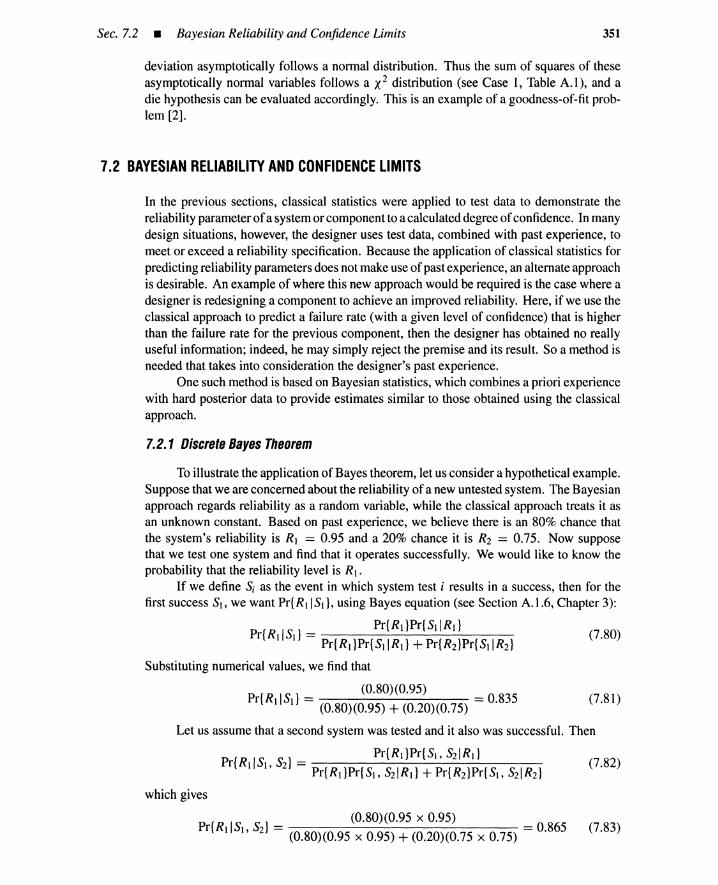
Sec. 7.2 • Bayesian Reliability and Confidence Limits 351
deviation asymptotically follows a normal distribution. Thus the sum of squares of theseasymptotically normal variables follows a X2 distribution (see Case I, Table A.I), and adie hypothesis can be evaluated accordingly. This is an example of a goodness-of-fit prob-lem [2].
7.2 BAYESIAN RELIABILITY AND CONFIDENCE LIMITS
In the previous sections, classical statistics were applied to test data to demonstrate thereliability parameter ofa system or component to a calculated degree of confidence. In manydesign situations, however, the designer uses test data, combined with past experience, tomeet or exceed a reliability specification. Because the application of classical statistics forpredicting reliability parameters does not make use of past experience, an alternate approachis desirable. An example of where this new approach would be required is the case where adesigner is redesigning a component to achieve an improved reliability. Here, if we use theclassical approach to predict a failure rate (with a given level of confidence) that is higherthan the failure rate for the previous component, then the designer has obtained no reallyuseful information; indeed, he may simply reject the premise and its result. So a method isneeded that takes into consideration the designer's past experience.
One such method is based on Bayesian statistics, which combines a priori experiencewith hard posterior data to provide estimates similar to those obtained using the classicalapproach.
7.2.1 Discrete Bayes Theorem
To illustrate the application of Bayes theorem, let us consider a hypothetical example.Suppose that we are concerned about the reliability of a new untested system. The Bayesianapproach regards reliability as a random variable, while the classical approach treats it asan unknown constant. Based on past experience, we believe there is an 80% chance thatthe system's reliability is R1 = 0.95 and a 20% chance it is R2 = 0.75. Now supposethat we test one system and find that it operates successfully. We would like to know theprobability that the reliability level is R I.
If we define S; as the event in which system test i results in a success, then for thefirst success Sl, we want Pr{R1IS1}, using Bayes equation (see Section A.l.6, Chapter 3):
Pr{RdSd = Pr{RdPr{SdRdPr{R I }Pr{SIIR1} + Pr{R2}Pr{SIIR2}
Substituting numerical values, we find that
Pr{R IS } = (0.80)(0.95) = 0.8351 1 (0.80)(0.95) + (0.20)(0.75)
(7.80)
(7.81)
Let us assume that a second system was tested and it also was successful. Then
Pr{R\IS\. Sz} = Pr{RdPr{S). SzlRd (7.82)Pr{R1}Pr{SI, S21 R I} + Pr{R2}Pr{SI, S21 R2}
which gives
P { IS S}(0.80)(0.95 x 0.95)
rRI 1,2= =0.865(0.80)(0.95 x 0.95) + (0.20)(0.75 x 0.75)
(7.83)
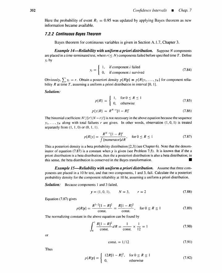
352 Confidence Intervals • Chap. 7
Here the probability of event R, == 0.95 was updated by applying Bayes theorem as newinformation became available.
7.2.2 Continuous Bayes Theorem
Bayes theorem for continuous variables is given in Section A.I.?, Chapter 3.
Example 14-Reliability with uniform a priori distribution. Suppose N componentsare placed in a time-terminated test, wherer(~ N) components failed before specified time T. DefineYi by
v. = { I,.1 0,
if component i failed
if component i survived(7.84)
Obviously, LYi = r. Obtain a posteriori density p{RIY} == p{RIYI, ... , YN} for component relia-bility R at time T, assuming a uniform a priori distribution in interval [0, I].
Solution:
{I, for°~ R ~ I
p{R} =0, otherwise
p{yIR} = RN-'[l - RY
(7.85)
(7.86)
The binomial coefficient N !/[r! (N - r)!] is not necessary in the above equation because the sequenceYI, ... ,YN along with total failures r are given. In other words, observation (I, 0, I) is treatedseparately from (I, 1,0) or (0, I, I).
RN-'[I - R]'p{RIY} = , forO ~ R ~ I (7.87)f [numerator]dR
This a posteriori density is a beta probability distribution [2,3] (see Chapter 6). Note that the denom-inator of equation (7.87) is a constant when y is given (see Problem 7.5). It is known that if the apriori distribution is a beta distribution, then the a posteriori distribution is also a beta distribution; inthis sense, the beta distribution is conserved in the Bayes transformation. •
Example IS-Reliability with uniform a priori distribution. Assume that three com-ponents are placed in a 10 hr test, and that two components, I and 3, fail. Calculate the a posterioriprobability density for the component reliability at 10 hr, assuming a uniform a priori distribution.
Solution: Because components I and 3 failed,
y=(I,O,I),
Equation (7.87) gives
R3- 2[1 _ R]2p{RlYl = ----
const.
N =3,
R[l - R]2
const.
r=2
for°~ R ~ I
(7.88)
(7.89)
The normalizing constant in the above equation can be found by
11 R[l - Rf I I----dR= -- x - = 1
() const. const. 12
or
const. = 1/12
Thus
(7.90)
(7.91)
{12R[1 - R]2,
p{RIY} =0,
forO ~ R ~ 1
otherwise(7.92)
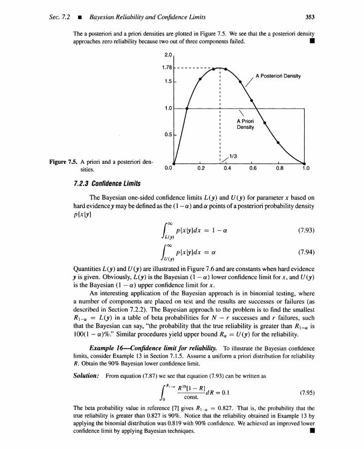
Sec. 7.2 • Bayesian Reliability and Confidence Limits 353
The a posteriori and a priori densities are plotted in Figure 7.5. We see that the a posteriori densityapproaches zero reliability because two out of three components failed. •
2.0
1.00.80.6
/ A Posteriori Density
\A PrioriDensity
0.4
-: 1/3
0.20.0
0.5
1.0 ....-- -----4------~-----__,
1.5
1.78
Figure 7.5. A priori and a posteriori den-sities.
7.2.3 Confidence Limits
The Bayesian one-sided confidence limits L(y) and U(y) for parameter x based onhard evidence y may be defined as the (1 - ex) and ex points of a posteriori probability densityp{xIY}
tx) p{xlYldx = 1 - ex (7.93)lL(Y)
100 p{xlYldx = ex (7.94)U(y)
Quantities L (y) and U(y) are illustrated in Figure 7.6 and are constants when hard evidencey is given. Obviously, L(y) is the Bayesian (1 - ex) lower confidence limit for x, and U (y)is the Bayesian (1 - ex) upper confidence limit for x.
An interesting application of the Bayesian approach is in binomial testing, wherea number of components are placed on test and the results are successes or failures (asdescribed in Section 7.2.2). The Bayesian approach to the problem is to find the smallestR1- ex == L(y) in a table of beta probabilities for N - r successes and r failures, suchthat the Bayesian can say, "the probability that the true reliability is greater than RI-.o is1OO( 1 - ex)%." Similar procedures yield upper bound Rex == U (y) for the reliability.
Example 16-Confidence limit for reliability. To illustrate the Bayesian confidencelimits, consider Example 13 in Section 7.1.5. Assume a uniform a priori distribution for reliabilityR. Obtain the 90% Bayesian lower confidence limit.
(7.95)
Solution: From equation (7.87) we see that equation (7.93) can be written ast R19[1 - R]----dR=O.1
o const.
The beta probability value in reference [7] gives R1- a = 0.827. That is, the probability that thetrue reliability is greater than 0.827 is 90%. Notice that the reliability obtained in Example 13 byapplying the binomial distribution was 0.819 with 90% confidence. We achieved an improved lowerconfidence limit by applying Bayesian techniques. •

354 Confidence Intervals _ Chap. 7
Upper1 Confidence11- Limit
1111111
Confidence1 -2a
LowerConfidence 1 Confidence Interval
Limit ----I·
'---_-...:;__--I""- -"--'__..-.;a, X
L(y) U(y)
Figure 7.6. Bayesian confidence limits.
The Bayesian approach applies to confidence limits for reliability parameters such asreliability, failure rate, and mean time to failure. The reader is referred to [3,8] for details.
REFERENCES
[1] John, P. W. M. Statistical Methods in Engineering and Quality Assurance. New York:John Wiley & Sons, 1990.
[2] Kececioglu, D. Reliability & Life Testing Handbook, Volume J. Englewood Cliffs, NJ:Prentice Hall, 1993.
[3] Mann, N. R. R., R. E. Schafer, and N. D. Singpurwalla. Methodsfor Statistical AnalysisofReliability and Life Data. New York: John Wiley & Sons, 1974.
[4] Catherine, M. T. "Tables of the percentage points of the X2 distribution," Biometrika,vol. 32, pp. 188-189, 1941.
[5] Bayer, W. H. (ed.). Handbook ofTables for Probability and Statistics (2d ed.). Cleve-land, OH: The Chemical Rubber Company, 1968.
[6] Burington, M. Handbook of Probability and Statistics, with Tables. New York:McGraw-Hill, 1953.
[7] Harter, H. L. New Tables ofthe Incomplete Gamma-Function Ratio and ofPercentagePoints ofthe Chi-Square and Beta Distribution. Washington, D.C.: U.S. GovernmentPrinting Office, 1964.
[8] Maltz, H. F., and R. A. Waller. Bayesian Reliability Analysis. New York: John Wiley& Sons, 1992.
CHAPTER SEVEN APPENDIX
A.1 THEX-, STUDENT'S t, AND FDISTRIBUTIONS
These three distributions are summarized in Tables A7.1, A7.2, and A7.3, which show theheadings of distribution, random variable, degrees of freedom, probability density function(Pdf.), mean, variance, three application modes (Case I to Case 3), and asymptotic distri-

Appendix A.l • The x2, Student's t, and F Distributions 355
bution for large degrees of freedom. For the application mode rows, random variables areassumed to be independent. Figures A7.1, A7.2, and A7.3 show probability density graphsand percentage points.
TABLE A7.1. Summary of X2 Distributions
Distributions ~Descriptions ~ x: Distribution
Name csq*(v)Variable o :s X2
Degrees of freedom o < v: integer
ra]. 1 (2) J-1 e-(x2)/22v/ 2r(v/2) X
Mean X2 = v
Variance a 22 = 2v
x
Case 1 Xl, ... , X; '" gau*(O, I)-U-
X2 == Xi + ... + X; '" csq*(n)
Case 2 Xl, ... , X; '" gau*(jl, a)- 1 z=nX ==;; ;=1 Xi: sample mean
s2 == n~l Z=;==l (Xi - X)2: sample var.
-U-
(n - I)S2/a 2 '" csq*(n - I)
Case 3 TI , ••• .T; rv exp*()...)
-U-
2ATI '" csq*(2)
2)", Z=;=2 T; '" csq* (2n - 2)
2)... Z=;=1 T; '" csq*(2n)
2)", [(n - -vt; + Z=~=1 T;] '" csq*(2r), T; : ordered
( 2Y/3 (2 2)v ~ 00 !:- '" gau* I - -, -v 9v 9v
(2X 2)1/2 rv gau*«2v - 1)1/2, 1), v ~ 100
A. 1.1 t Distribution Application Modes
Case1. The sum of squares of normal random variables follows a X2 distribution.This fact is used, for example, for a goodness-of-fit problem. Note that many randomvariables are approximated asymptotically by a normal random variable. Variable symbolX2 suggests the random variable squared.
Case 2. A ratio of sample variance to true variance for a normal population followsa X2 distribution. A confidence interval of the true variance is obtained.
Case 3. The sum of an exponentially distributed random variable follows a X2
distribution. A confidence interval of the mean time to failure is obtained. Notice thatthe exponential variables in the first three equations are not ordered in ascending order. On
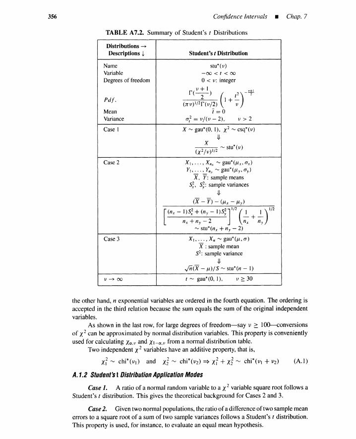
356 Confidence Intervals • Chap. 7
TABLE A7.2. Summary of Student's t Distributions
Distributions --+
Descriptions ~ Student's t Distribution
Name stu*(v)Variable -00 < t < 00
Degrees of freedom o< v: integer
r(v+ 1) _I'tl
ra]. 2 ( (2).1+-(rrv) 1/2r(v/2) v
Mean 1=0Variance a? = v/(v - 2), v > 2
Case 1 X "'-.; gau*(O, I), X2 "'-.; csq*(v)
-U-
X *2 1/2 "'-.; stu (v)
(X Iv)
Case 2 XI, ... , Xnx "'-.; gau*(JLx, ax)Yl , ... , Yn y "'-.; gau*(JLy, ay)
X, Y: sample means5.;, 5;: sample variances
-U-
(X- Y) - (JLx - JLy)
[ 2 2f2 ( y/2(nx - 1)5.t + (fly - 1)5y ~ + ~
fl x + fly - 2 n; fly"'-.; StU*(flx + fly - 2)
Case 3 Xl, ... , Xn "'-.; gau*(JL, a)
X :sample mean52: sample variance
-U-~(X - JL)/5 "'-.; stu*(n - I)
v ~ 00 t "'-.; gau*(O, I), v ~ 30
the other hand, n exponential variables are ordered in the fourth equation. The ordering isaccepted in the third relation because the sum equals the sum of the original independentvariables.
As shown in the last row, for large degrees of freedom-say v :::: 1DO-conversionsof X2can be approximated by normal distribution variables. This property is convenientlyused for calculating Xa,v and XI-a,v from a normal distribution table.
Two independent X2 variables have an additive property, that is,
x~ ~ chi*(vl) and xi rv chi*(v2) => X~ + xi r<» chi*(vi + V2) (A.I)
A.1.2 Student's t Distribution Application Modes
Case1. A ratio of a normal random variable to a X2 variable square root follows aStudent's t distribution. This gives the theoretical background for Cases 2 and 3.
Case2. Giventwo normalpopulations, the ratio of a differenceof two sample meanerrors to a square root of a sum of two sample variances follows a Student's t distribution.This property is used, for instance, to evaluate an equal mean hypothesis.
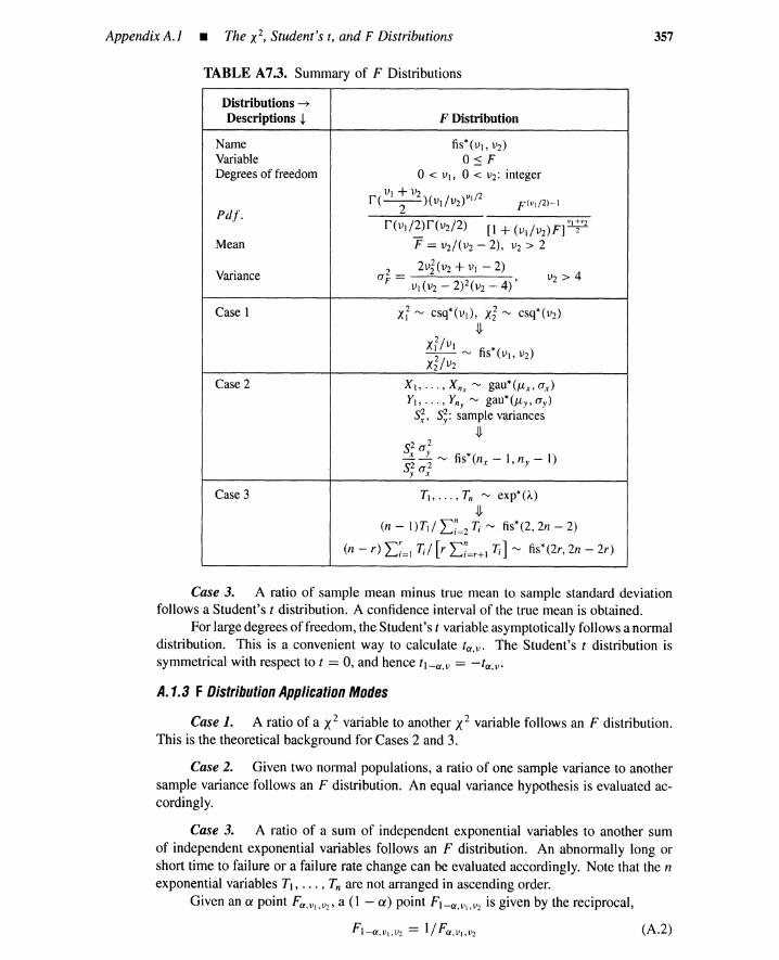
Appendix A.l • The X2, Student's t, and F Distributions
TABLE A7.3. Summary of F Distributions
357
Distributions --+
Descriptions ~
NameVariableDegrees of freedom
Pdf·
Mean
Variance
Case 1
Case 2
Case 3
F Distribution
fis* (VI, V2)o~ F
o< VI, 0 < V2: integer
r(VI + V2)(VI/V2)V1/22 F(V1/2)-I
r(vI/2)f(V2/2) [I + (Vl/V2)F] \'1;\02
F = V2/ (V2 - 2), V2 > 2
2 2vl(V2 + VI - 2)a F = , v2>4
VI(V2 - 2)2(V2 -4)
Xl, ... , X nx "'V gau*(Jlx, ax)Y1, ••• , Yn y "'V gau*(Jly,a y)
s.;, S;: sample variances-U-
S2 a 2
--:!.-L"'V fis*(nx-l,ny-l)S; a;T1, ••• .T; "'V exp*(),,)
-U-(n - 1)T1/ I:;=2 T; "'V fis*(2,2n - 2)
(n - r) I:~=l T;/ [r I:;=r+l T;] "'V fis*(2r, 2n - 2r)
Case 3. A ratio of sample mean minus true mean to sample standard deviationfollows a Student's t distribution. A confidence interval of the true mean is obtained.
For large degrees of freedom, the Student's ( variable asymptotically follows a normaldistribution. This is a convenient way to calculate ta ,v- The Student's t distribution issymmetrical with respect to t == 0, and hence tl-a,v == -(a,v.
A.1.3 FDistribution Application Modes
Case 1. A ratio ofaX2 variable to another X2 variable follows an F distribution.This is the theoretical background for Cases 2 and 3.
Case 2. Given two normal populations, a ratio of one sample variance to anothersample variance follows an F distribution. An equal variance hypothesis is evaluated ac-cordingly.
Case 3. A ratio of a sum of independent exponential variables to another sumof independent exponential variables follows an F distribution. An abnormally long orshort time to failure or a failure rate change can be evaluated accordingly. Note that the nexponential variables T1, ••• , T; are not arranged in ascending order.
Given an a point Fa , V 1, V2 ' a (1 - a) point FI - a , V1 , V2 is given by the reciprocal,
(A.2)
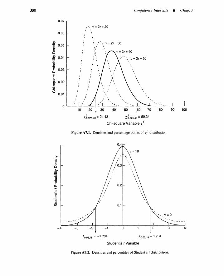
358
0.07
0.06
~'en 0.05c0)
0
~ 0.04:0
ct:S.c0 0.03...
C-O)
co::J 0.020-cr:co
0.01
o
,-, v =2r= 20, \
1 \
I \I \I \
: ", v =2r= 30I \'
I )'
I I'I 1 \
I I \I \
I : \
I I \I \
I " \I \
I I' \
I II II I
I II ,
, I1 ,I ,, ,, ,
, I
Confidence Intervals • Chap. 7
" v =2r= 50,,,,,,,,,,,,\ ,,, ,
" "
X~.975,40 =24.43 X~.025,40 =59.34
Chi-square Variable X2
Figure A7.1. Densities and percentage points of X2 distribution.
0.4
-4 -3 -2 -1
0.2
0.1
o
v =18,,,,,,
\\,,,
\
\ ,,,,,,\
\
"
2
v=2
3 4
t0.95,18 = -1.734 t0.05,18 = 1.734
Student's t Variable
Figure A7.2. Densities and percentiles of Student's t distribution.
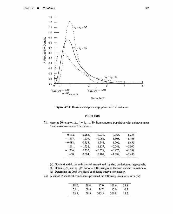
359
F O.05,15,15 =2.40
5432
, ,I \
I \
l, v1= v2=35I \
I II ,I ,
I II ,
I \
\
I
v1'.=v2 =15\I
\\\\\\
\
0.0 0
FO.95.15.15 =0.42=1/ FO.05,15,15
Chap. 7 • Problems
1.3
1.2
1.1
1.0
?:- 0.9'wc 0.8OJ0g 0.7
:c 0.6ell.ce 0.5o,u, 0.4
0.3
0.2
0.1
Var iable F
Figure A7.3. Densities and percentage points of F distribution.
PROBLEMS
7.1. Assume 30 samples, Xi, i = 1, ... ,30, from a normal population with unknown mean() and unknown standard deviation a :
-0.112, - 0.265, -0.937, 0.064, 1.236-1.317, -1 .239, -0.061, 1.508, -1.165-0.082, 0.254, 1.742, 1.706, -1 .659
1.211, -1 .532, 1.127, -0.741, -0.097-1.736, 0.252, -0.379, -0.875, -0.598
1.600, 0.694, 0.401, -1 .098, -0.430
(a) Obtain eand (j, the estimates of mean () and standard deviat ion a, respectively.(b) Obtain .l'a«() and .l'1- a «() for ex =0.05, using ii as the true standard deviation a .(c) Determine the 90% two-sided confidence interval for mean ().
7.2. A test of 15 identical components produced the following times to failures (hr):
118.2,55.1,25.5,
128.4,68.5,
158.5,
17.0,74.7,
335.5,
161.6,15.0,
306.8,
33.80.7
15.2
360 ConfidenceIntervals _ Chap. 7
(a) Obtain the times to failures for time-terminated test with T = 70.
(b) Obtain the times to failures for failure-terminated test with r = 10.
(e) Find the 90% two-sided confidence interval of MTfF for failure-terminated test,assuming an exponential failure distribution and the chi-square table:
Pr{x2~~(V)} = a
ex = 0.975 ex = 0.950 ex = 0.05 ex = 0.025
v = 10 3.247 3.940 18.31 20.48
v = 15 6.262 7.261 25.00 27.49
v = 20 9.591 10.851 31.41 34.17
(d) Obtain 90% confidence intervals for the component failure rate A and componentreliability at t = 100, assuming a failure-terminated test.
7.3. A total of ten identical components were tested using time-terminatedtest with T = 40(hr). Four components failed during the test. Obtain algebraic equations for 95% upperand lower confidence limits of the component reliability at t = 40 (hr).
7.4. Assume that we are concerned about the reliability of a new system. Past experiencegives the followinga priori information.
Reliability Probability
R1 = 0.98
R2 = 0.78
R) = 0.63
0.6
0.3
0.1
1 ::sNO::s r S N,
Now suppose that we test the two systems and find that the first system operates suc-cessfully and the second one fails. Determine the probability that the reliability level isR; (i = I, 2, 3), based on these two test results.
7.5. An a priori probability density of reliability R is given by
RN-r[l - R)'p{R} = ,
const.
Prove that the constant is
r!(N + I)N(N - I) x ... x (N - r + 1)
7.6. A failure-terminated test of 100 components resulted in a component failure within 200hr.(a) Obtain an a posterioriprobabilitydensity p{ Rly} of the component reliabilityat 200
hr, assuming an a priori density information:
R28[1 - R)2p{R}=----
const.
(b) Obtain the mean values of the reliability that distributes according to p{R} andp{ Rly}, respectively.
(e) Obtain reliabilities Rand RIY that maximize p{R} and p{Rly}, respectively.(d) Graph p{R} and p{RIY}.
Chap. 7 • Problems
7.7. Consider an a posteriori probability density
RN-'[l - RYp{Rly} =----
const.
Prove that:(a) The mean value Rly of R is
- N-r+lRly= N+2
(b) The value R\y that maximizes p{R Iy} is
A N-rR Iy = ---;;;-
7.8. Prove the identities
N N'I - " . RN-s[l - RaY
L.J (N - s)!s! as=s
N! iRa= uN-S(1 _ u)S-ldu,(N - S)! (S - I)! 0
S N'1 - " . RN-s[1 - R ]SL.J (N _ )' ,I-a I-a
s=O S .s.
N! i I-
R1-
a
= uS(1 _ U)N-S-IduS!(N-S-I)! 0 '
7.9. The beta probability density with integer parameters ex, f3 is defined by
p{u} = (a +a~f3~ I)! u"[1 - u]fJ, 0 < u < I
361
(S =1= 0)
(5 =1= N)
Prove that:(a) The upper confidence limit R; in (7.70) satisfies the following probability equation,
where X is a beta distribution variable with parameters [N - S, S - I]. (For upperbound R; for Problem 7.3, the beta distribution has parameters 6 and 3.)
PrIX ~ Ral = I - ex
(b) The lower confidence limit R I - a in (7.72) satisfies the following probability equa-tion, where X is a beta distribution variable with parameters [5, N - 5 - I]. (Forlower bound R I - a for Problem 7.3, the beta distribution has parameters 4 and 5.)
PrIX ~ I - RI-al = I - ex
7.10. The F distribution with 2k and 2[ degrees of freedom has the probability density
(k + [ - I)' ( k ) k k{F} = . - Fk-I(I + _F)-k-lP (k - I)!([ - I)! [ /
Show that when V is distributed with the beta distribution with parameters k - 1 andl - I, then the distribution of the new random variable
[ VU=-x--
k 1- V
is an F distribution with 2k and 2/ degrees of freedom.
7.11. Obtain the upper and lower bounds of the component reliability in Problem 7.3, usingthe results of Problems 7.9 and 7.1O. Assume an F distribution table with VI and V2
degrees of freedom. Interpolate FO.05 values if necessary:

362 Confidence Intervals - Chap. 7
Pr{F ::: Fo.os} =0.05
V2 = 8V2 = 10
V2 = 12
VI = 10
3.347
2.978
2.753
VI = 12
3.284
2.913
2.687
VI = 15
3.218
2.845
2.617
7.12. A component reliability has the a posteriori distribution
R5 ( 1 - R)4p{RIY}=---
const.
Obtain the 90% confidence reliability for R.
uantitative Aspectsof System Analysis
8.1 INTRODUCTION
Chapters 6 and 7 deal with the quantification of basic events. We now extend these methodsto systems.
System success or failure can be described by a combination of top events definedby an OR combination of all system hazards into a composite fault tree (Figure 8.1). Thenon-occurrence of all system hazards implies system success. In general, we can analyzeeither a particular system hazard or a system success by an appropriate top event and itscorresponding fault tree.
The following probabilistic parameters describe the system. Their interpretationdepends on whether the top event refers to a system hazard or an OR combination of thesehazards.
1. System availability As(t) = probability that the top event does not exist at timet. Subscript s stands for system. This is the probability of the system's operat-ing successfully when the top event refers to an OR combination of all systemhazards. It is the probability of the non-occurrence of a particular hazard whenthe top event is a single system hazard.
2. System unavailability Qs(t) = probability that the top event exists at time t.This is either the probability of system failure or the probability of a particularsystem hazard at time t, depending on the definition of the top event. The systemunavailability is complementary to the availability, and the following identityholds:
(8.1)
363
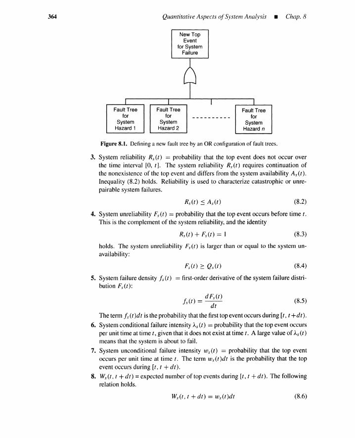
364 Quantitative Aspects ofSystem Analysis _ Chap. 8
New TopEvent
for SystemFailure
Fault Treefor
SystemHazard 1
Fault Treefor
SystemHazard 2
Fault Treefor
SystemHazard n
Figure 8.1. Defininga new fault tree by an OR configurationof fault trees.
3. System reliability R.\. (t) == probability that the top event does not occur overthe time interval [0, tl. The system reliability Rs(t) requires continuation ofthe nonexistence of the top event and differs from the system availability As(r).Inequality (8.2) holds. Reliability is used to characterize catastrophic or unre-pairable system failures.
(8.2)
4. System unreliability F'.\. (t) == probability that the top event occurs before time t.This is the complement of the system reliability, and the identity
Rs (t) + F'.11 (t) == 1 (8.3)
holds. The system unreliability Fs(t) is larger than or equal to the system un-availability:
(8.4)
5. System failure density !\. (t) == first-orderderivative of the system failure distri-bution Fs(t):
d F'.\.(t)I. (t) == --;Jt (8.5)
The term !\.(t)dt is the probability that the first top event occurs during [r, t +dt).
6. System conditional failure intensity A.\. (z) == probability that the top event occursper unit time at time t, given that it does not exist at time t. A large value of As(t)means that the system is about to fail.
7. System unconditional failure intensity ws(t) == probability that the top eventoccurs per unit time at time t. The term ws(t)dt is the probability that the topevent occurs during [t, t +dt).
8. W\' it, t +dt) = expected number of top events during [t, t +dt). The followingrelation holds.
(8.6)

Sec. 8.2 • Simple Systems 365
(8.9)
9. Ws(tl, t2) = expected number of top events during [tl, tz). This is given byintegration of the unconditional failure intensity ws(t):
Ws(tl, t2) = 1" ws(t)dt (8.7)t1
10. MTTFs = mean time to failure =expected length of time to the first occurrenceof the top event. The M1TFs corresponds to average lifetime and is a suitableparameter for catastrophic system hazards. It is given by
MTTFs =100
tfs(t)dt (8.8)
or
MTTFs = 100
Rs(t)dt, if Rs(oo) = 0
In this chapter we discuss mainly the system availability and unavailability: systemreliability and unreliability is quantified by Markov methods in Chapter 9. Unless otherwisestated, all basic events are assumed to be mutually independent. Dependent failures are alsodescribed in Chapter 9. We first demonstrate availability As(t) or unavailability Qs(t) =1 - As (r) calculations, given relatively simple fault trees. Quantification methods apply toreliability block diagrams and fault trees because both are modeled by Boolean functions.Next we discuss methods for calculating lower and upper bounds for the system unavailabil-ity Qs(r). Then we give a brief summary of the so-called kinetic tree theory [1], which is usedto quantify system parameters for large and complex fault trees. Two types of sensor system-failure probabilities, that is, failed-safe and failed-dangerous probabilities are developed.
As shown in Figure 4.16, each basic event is a component primary failure, a componentsecondary failure, or a command failure.
To simplify the nomenclature, we use capital letters B, BI, C, and so on, to representboth the basic events and their existence at time t. When event B is a component failure,the probability Pr{B} is the component unavailability Q(t).
Failure modes should be defined for component failures. Primary failures are causedby natural aging (random or wearout) within the design envelope. Environmental impacts,human error, or system-dependent stresses should be identified as possible causes of thesecondary failures that create transitions to the failed state. These failure modes and possiblecauses clarify the basic events and are necessary for successful reliability quantification.
8.2 SIMPLE SYSTEMS
8.2.1 Independent Basic Events
The usual assumption regarding basic events B I , ••• , B; is that they are independent,which means that the occurrence of a given basic event is in no way affected by the occur-rence of any other basic event. For independent basic events, the simultaneous existenceprobability Pr{B I n B2n ... n Bn } reduces to
Pr{B I n B2n··· n Bn } = Pr{B I}Pr{B2}·· ·Pr{Bn }
where the symbol n represents the intersection of events B I, ... , Bn •
(8.10)
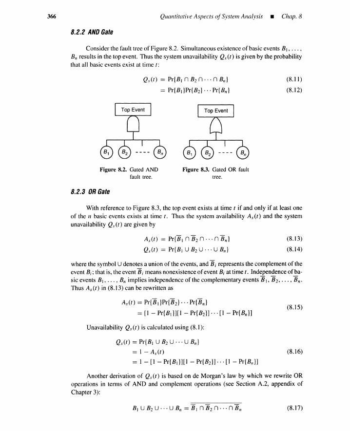
366 Quantitative Aspects ofSystem Analysis • Chap. 8
8.2.2 AND Gate
Consider the fault tree of Figure 8.2. Simultaneous existence of basic events B I , ••• ,
B; results in the top event. Thus the system unavailability Q.\. (t) is given by the probabilitythat all basic events exist at time t:
Q.\,(t) == Pr{B I n B2 n··· n Bn}
== Pr{B I }Pr{B2} ..• Pr{Bn }
(8.11)
(8.12)
Figure 8.2. Gated ANDfault tree.
8.2.3 OR Gate
Figure 8.3. Gated OR faulttree.
With reference to Figure 8.3, the top event exists at time t if and only if at least oneof the n basic events exists at time t. Thus the system availability As (z) and the systemunavailability Qs(t) are given by
As(t) == Pr(BI nB2n ... nBnl
Qs(t) == Pr{B I UB2U···UBn }
(8.13)
(8.14)
where the symbol U denotes a union of the events, and Bi represents the complement of theevent Bi ; that is, the event Bi means nonexistence of event B, at time t. Independence ofba-sic events B I , ••• , B; implies independence of the complementary events BI , B2' ... ,Bn .
Thus As(t) in (8.13) can be rewritten as
As(t) == Pr{B I }Pr{B2} •.• Pr{Bn}
== [1 - Pr{B I } ] [I - Pr{B2}] ••• [1 - Pr{e.}]Unavailability Qs(t) is calculated using (8.1):
(8.15)
Qs(t) == Pr{B I U B2 U··· U Bn}
== I - As(t) (8.16)
== I - [1 - Pr{B I }][1 - Pr{B2 } ] ••• [1 - Pr{Bn }]
Another derivation of Qs(t) is based on de Morgan's law by which we rewrite ORoperations in terms of AND and complement operations (see Section A.2, appendix ofChapter 3):
BI U B2 U··· U s, == B I n B2 n··· n s, (8.17)

Sec. 8.2 • Simple Systems
Thus
Qs(t) == Pr{EI n E2 n··· n En}== 1-Pr{EI nE2n ... nEn }
== 1 - [1 - Pr{BI}][1 - Pr{B2}]... [1 - Pr{Bn}]
For n == 2,
Qs(t) == Pr{BI U B2}
== Pr{BI} + Pr{B2} - Pr{BI1Pr{B21
367
(8.18)
(8.19)
(8.20)
(8.21)
In other words, the probability Qs(t) that at least one of the events BI and B2exists is equalto the sum of the probabilities of each event minus the probability of both events existingsimultaneously. This is shown by the Venn diagram of Figure 8.4. For n == 3,
Qs(t) == Pr{BI U B2 U B3}
== Pr{BI} + Pr{B21 + Pr{B31 - Pr{B I }Pr{B2} - Pr{B2}Pr{B31- Pr{B3}Pr{BI}+ Pr{BI}Pr{B2}Pr{B31
This unavailability is depicted in Figure 8.5. Equations (8.20) and (8.21) are special casesof the inclusion-exclusion formula described in Section 8.5.4.
Figure 8.4. Pr{Bd + Pr{B2} -Pr{BdPr{B2}'
8.2.4 Voting Gate
Figure 8.5. Illustration of formulafor Pr{B} U B2 U B3}.
The fault tree of Figure 8.6 appears in a voting system that produces an output ifm or more components out of n generate a command signal. A common application ofthe m-out-of-n system is in safety systems, where it is desirable to avoid expensive plantshutdowns by a spurious signal from a single safety monitor.
As an example, consider the two-out-of-three shutdown device of Figure 8.7. Plantshutdown occurs when two out of three safety monitors generate shutdown signals. Considera case where the plant is normal and requires no shutdown. An unnecessary shutdownoccurs if two or more safety monitors produce spurious signals. Denote by B; a false signalfrom monitor i, The resulting fault tree is shown in Figure 8.8, which is a special case ofFigure 8.6.
Although an m-out-of-n gate such as Figure 8.6 can always be decomposed intoequivalent AND and OR gates, direct application of the binomial Bernoulli distributionequations represents an alternative analytical approach.

368 Quantitative Aspects ofSystem Analysis _ Chap. 8
TopEvent
Figure 8.6. nz-out-of-n voting system.
PlantState
Monitor 1 CommandSignal 1
Command Voting ShutdownMonitor2
Signal 2 2/3
Monitor3 CommandSignal 3
Figure 8.7. Two-out-of-three shutdown system.
Figure 8.8. Fault tree for two-out-of-three shutdown system.
Assume that all basic events have the probability Q.
Pr{B1} = Pr{B2} = ... = Pr{Bn } = Q (8.22)
The binomial distribution gives the probability that a total of m outcomes will occur, giventhe outcome probability Q of anyone trial and the number of trials n:
Pr{m; n, QJ = ( ; ) Qm(l _ ar: (8.23)
This equation is derived by considering that one way of achieving In outcomes is tohavem consecutiveoccurrences,then (n -m) consecutivenon-occurrences. Theprobabilityof this sequence is Qm(1 - Q)n-m. The total number of sequences is the number of
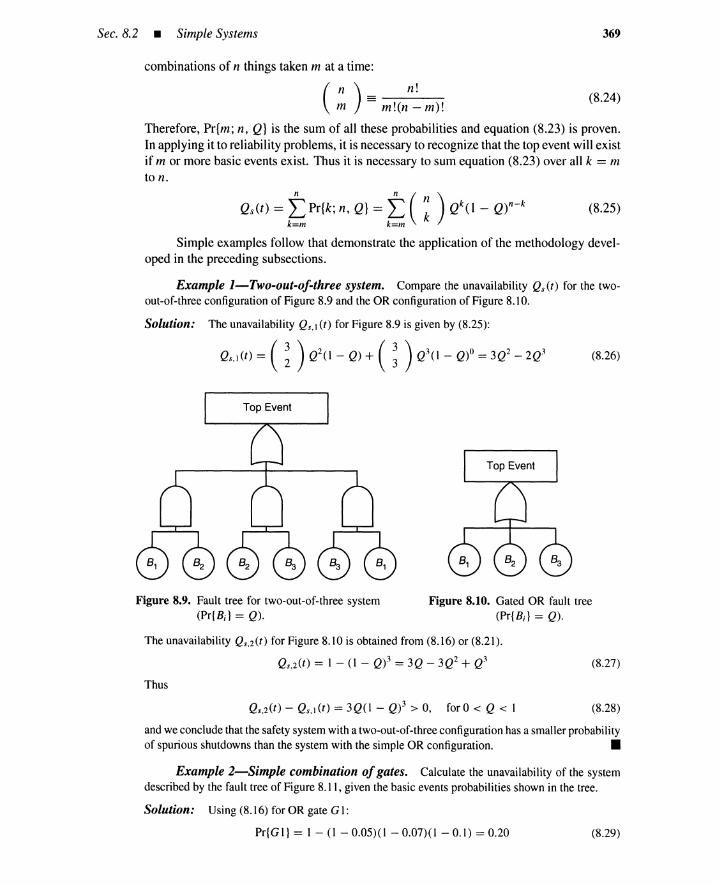
Sec. 8.2 • Simple Systems 369
(8.25)
combinations of n things taken m at a time:
( ; ) == m!(nn~ m)! (8.24)
Therefore, Pr{m; n, Q} is the sum of all these probabilities and equation (8.23) is proven.In applying it to reliability problems, it is necessary to recognize that the top event will existif m or more basic events exist. Thus it is necessary to sum equation (8.23) over all k == m
to n.
Qs(t) = 1;;, Pr{k; n, Q} = 1;;, ( : ) Qk(l - or:Simple examples follow that demonstrate the application of the methodology devel-
oped in the preceding subsections.
Example I-Two-out-of-three system. Compare the unavailability Qs(t) for the two-out-of-three configuration of Figure 8.9 and the OR configuration of Figure 8.10.
Solution: The unavailability Qs.1(t) for Figure 8.9 is given by (8.25):
Qs.I(t) = ( ~ ) Q2(l - Q) + ( ~ ) Q3(l - Q)o = 3Q2 - 2Q3 (8.26)
Figure 8.9. Fault tree for two-out-of-three system(Pr{ B;} = Q).
Figure 8.10. Gated OR fault tree(Pr{B;} = Q).
The unavailability Qs,2(t) for Figure 8.10 is obtained from (8.16) or (8.21).
Qs,2(t) = I - (I - Q)3 = 3Q - 3Q2 + Q3
Thus
Qs,2(t) - Qs,1 (t) = 3Q(1 - Q)3 > 0, for 0 < Q < I
(8.27)
(8.28)
and we conclude that the safety system with a two-out-of-three configuration has a smaller probabilityof spurious shutdowns than the system with the simple OR configuration. •
Example 2-Simple combination ofgates. Calculate the unavailability of the systemdescribed by the fault tree of Figure 8.11, given the basic events probabilities shown in the tree.
Solution: Using (8.16) for OR gate G 1:
Pr{Gl} = 1 - (1 - 0.05)(1 - 0.07)(1 - 0.1) = 0.20 (8.29)

370 Quantitative Aspects ofSystem Analysis _ Chap. 8
0.01
0.09 0.09 0.09 0.05 0.07 0.1
Figure 8.11. Simple combination of gates.
For the two-out-of-threegate G2, by (8.25):
Pr{G2) == t (i )0.09*(1 - 0.09)3-*
_(3) 2 (3) 3 0- 2 0.09 (I - 0.09) + 3 0.09 (I - 0.09)
= 0.023
Using (8.12) for AND gate G3:
Qs(t) = Pr{G3} = Pr{GI}Pr{G2}Pr{D}
= (0.20)(0.023)(0.01) = 4.6 x 10- 5
(8.30)
(8.31)
(8.32)
•Example 3-Tail-gas quench and clean-up system [2]. The system in Figure 8.12 is
designed to: I) decrease the temperatureof a hot gas by a waterquench, 2) saturate the gas with watervapor,and 3) remove solid particles entrained in the gas.
A hot "tail" gas from a calciner is first cooled by contacting it with water supplied by quenchpumps B or C. It then passes to a prescrubber where it is contacted with more fresh water suppliedby feedwater pump D. Water from the bottom of the prescrubber is either recirculated by pumps Eor F or removed as a purge stream. Mesh pad G removes particulates from the gases that flow to anabsorber after they leave the prescrubber.
A simplifiedfault tree is shown in Figure 8.13. The booster fan (A), both of the quench pumps(B and C), the feedwater pump (D), both of the circulation pumps (E and F), or the filter system (G)must fail for the top event T to occur. The top event expression for this fault tree is
T = A U (8 n C) U D U (E n F) U G
Calculate the system unavailability Qs(t) = Pr{T} using as data:
(8.33)
Pr{A} = 0.9,
Pr{E} = 0.5,
Pr{B} = 0.8,
Pr{F} = 0.4,
Pr{C} = 0.7,
PriG} = 0.3
Pr{D} = 0.6,(8.34)
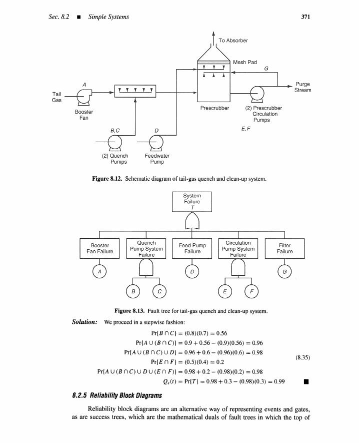
Sec. 8.2 • Simple Systems 371
PurgeStream
(2) Prescru bberCirculationPumps
Prescrubber
T T T T T I----t--~
~====::::::=l Mesh Pad
Booste rFan
Tai lGas
o E,F
(2) QuenchPumps
FeedwaterPump
Figure 8.12. Schematic diagram of tail-gas quench and clean-up system.
SystemFailure
T
FilterFailure
CirculationPump System
Failure
Feed PumpFailure
QuenchPump System
Failure
BoosterFan Failure
Figure 8.13. Fault tree for tail-gas quench and clean-up system.
Solution: We proceed in a stepwise fashion:
Pr(B n C} = (0.8)(0.7) = 0.56
Pr(A U (B n C)} = 0.9 + 0.56 - (0.9)(0.56) = 0.96
Pr(A U (B n C) U D} = 0.96 + 0.6 - (0.96)(0 .6) = 0.98
Pr(E n F} = (0.5)(0.4) =0.2
Pr(A U (B n C) U D U (E n F)} = 0.98 + 0.2 - (0.98)(0 .2) =0.98
Qs(t) = Pr(T} = 0.98 + 0.3 - (0.98)(0 .3) = 0.99
(8.35)
•8.2.5 Reliability Block Diagrams
Reliability block diagrams are an alternative way of representing events and gates,as are success trees, which are the mathematical duals of fault trees in which the top of
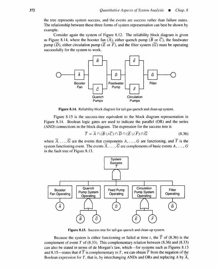
372 Quantitative Aspects ofSystem Analysis • Chap. 8
the tree represents system success, and the events are success rather than failure states.The relationship between these three forms of system representation can best be shown byexample.
Consider again the system of Figure 8.12. The reliability block diagram is givenas Figure 8.14, where the booster fan (A), either quench pump (8 or C), the feedwaterpump (D), either circulation pump (E or F), and the filter system (G) lTIUSt be operatingsuccessfully for the system to work.
BoosterFan
FeedwaterPump
Filter
QuenchPumps
CirculationPumps
Figure 8.14. Reliability block diagram for tail-gas quench and clean-up system.
Figure 8.15 is the success-tree equivalent to the block diagram representation inFigure 8.14. Boolean logic gates are used to indicate the parallel (OR) and the series(AND) connections in the block diagram. The expression for the success tree is
T == An (8 U C) n D n (E U F) n G (8.36)
where A, ... , G are the events that components A, ... , G are functioning, and T is thesystem functioning event. The events A, ... , G are complements of basic events A, ... , Gin the fault tree of Figure 8.13.
SystemSuccessr
FilterOperating
CirculationPump System
Operating
Feed PumpOperating
QuenchPump System
Operating
BoosterFan Operating
Figure 8.15. Success tree for tail-gas quench and clean-up system.
Because the system is either functioning or failed at time t, the T of (8.36) is thecomplement of event T of (8.33). This complementary relation between (8.36) and (8.33)can also be stated in terms of de Morgan's law, which-for systems such as Figures 8.13and 8.15-states that if T is complementary to T, we can obtain T from the negation of theBoolean expression for T, that is, by interchanging ANDs and ORs and replacing A by A,

Sec. 8.2 • Simple Systems 373
B by E, and so forth. This is proven by examining (8.33) and (8.36) or Figures 8.13 and8.15.
The system availability As(t) is calculated from the probability Pr{T} in the followingway.
From (8.34) in Example 3:
Hence
Pr{A} == 0.1,
Pr{E} == 0.5,
Pr{E} == 0.2,
Pr{F} == 0.6,
Pr{el == 0.3,
Pr{G} == 0.7
Pr{D} == 0.4,(8.37)
As(t) == Pr{T}
== (0.1)[0.3 + 0.2 - (0.3)(0.2)](0.4)[0.6 + 0.5 - (0.6)(0.5)](0.7) (8.38)
== 0.0099
The availability and the unavailability in the preceding example agree with identity (8.1)within round-off errors:
As(t) + Qs(t) == 0.0099 + 0.99 == 0.9999 ~ 1 (8.39)
The foregoing examples show that:
1. A parallel reliability block diagram corresponds to a gated AND fault tree, and aseries block diagram to a gated OR fault tree (Table 8.1).
TABLE 8.1. Reliability Block Diagram Versus Fault Tree
Reliability Block Diagram Fault Tree
Pr{B1nB2 } =Pr{BdPr{B-;} Pr{B 1uB2} =Pr{Bd+ Pr{B2}- Pr{B1}Pr{B2}
Pr{B1uB2} =Pr{B~} + Pr(B2} Pr{B 1nB2} =Pr{BdPr{B2}- Pr{B1}Pr{B2l

374 Quantitative Aspects ofSystem Analysis _ Chap. 8
2. The unavailability calculation methods for fault trees can be extended directlyto availability calculations for success trees when basic events B}, ... , B; arereplaced by their complementary events B}, ... ,», in (8.10) and (8.16):
n
Pr{BI n B2 n··· n B n} == DPr{B;};=}
n
Pr{B} UB2U ... UBn} == 1- D[I-Pr{B;}];=}
n
1- DPr{B;};=1
(8.40)
(8.41)
(8.42)
8.3 TRUTH·TABLE APPROACH
A truth table is a listing of all combinations of basic event states, the resulting existence ornonexistence of a top event, and the corresponding probabilities for these combinations. Asummation of a set of probabilities in the table yields the system unavailability Q.\, (t), anda complementary summation gives the system availability A.\, (t).
8.3.1 AND Gate
Table 8.2 is a truth table for the system of Figure 8.16. The system unavailabilityQ.\.(t) is given by row I:
TABLE 8.2. Truth Table for Gated AND Fault Tree
Basic Event B 1 Basic Event B2 Top Event Probability
1 Exists Exists Exists Pr{BdPr{B2}
2 Exists Not Exist Not Exist Pr{B t}Pr{B2}3 Not Exist Exists Not Exist Pr{B t}Pr{B2}4 Not Exist Not Exist Not Exist Pr{B tIPr{B2}
(8.43)
Figure 8.16. Gated AND fault tree.
8.3.2 OR Gate
Figure 8.17. Gated OR fault tree.
The system of Figure 8.17 is represented by the truth table of Table 8.3. The unavail-ability Q.\. (t) is obtained by a summation of the probabilities of the mutually exclusive rows1,2, and 3.

Sec.8.3 • Truth-Table Approach
TABLE 8.3. Truth Table for Gated OR Fault Tree
Basic Event B1 Basic Event B2 Top Event Probability
I Exists Exists Exists Pr{B}}Pr{B2 }
2 Exists Not Exist Exists Pr{B} }Pr{B2 }
3 Not Exist Exists Exists Pr{BdPr{B2 }
4 Not Exist Not Exist Not Exist Pr{B} }Pr{B2 }
Qs(t) = Pr{BI1Pr{B21 + Pr{BI1Pr{B2} + Pr{Bl}Pr{B21
=Pr{B l }Pr{B2} + Pr{Bl }[1 - Pr{B2}] + [1 - Pr{Bl }]Pr{B2}
= Pr{B 1} + Pr{B21- Pr{B11Pr{B21
This confirms equation (8.20).
375
(8.44)
Example 4-Pump-filter system. A truth table provides a tedious but reliable techniquefor calculating the availability and unavailability for moderately complicated systems, as illustratedby the following example.*
A plant has two identical, parallel streams, A and B, consisting of one transfer pump and onerotary filter (Figure 8.18). The failure rate of the pumps and filters are, respectively, 0.04 and 0.08failures per day, whether equipment is in operation or standby. Assume MTTRs for the pumps andfilters of 5 and 10 hr, respectively.
Stream APump A' Filter A"
Output
Stream BPump a' Filter a"
Figure 8.18. Two parallel process streams.
Two alternative schemes to increase plant availability are:
1. Add a third identical stream, C (Figure 8.19).
2. Install a third transfer pump capable of pumping slurry to either filter (Figure 8.20).
Stream APump A'
Stream BPump a'
Stream CPump e'
Filter A"
Filter a"
Filter c'
Output
Figure 8.19. Three parallel process streams.
*Courtesy of B. Bulloch, ICI Ltd., Runcom, England.
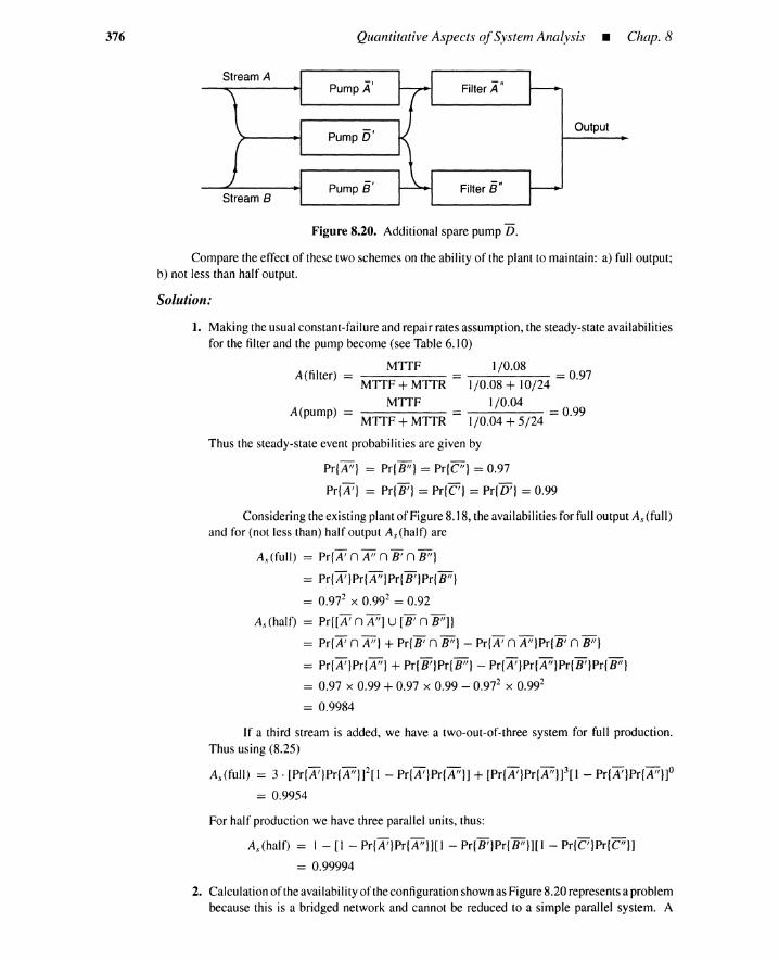
376 Quantitative Aspects ofSystem Analysis _ Chap. 8
Pump A'
Pump 0'
Pump a'
Filter A"
Filter a"
Output
Figure 8.20. Additional spare pump D.
Compare the effect of these two schemes on the ability of the plant to maintain: a) full output;b) not less than half output.
Solution:
1. Making the usual constant-failure and repair rates assumption, the steady-state availabilitiesfor the filter and the pump become (see Table 6.10)
A(filter) = MlTF 1/0.08 = 0.97MTTF + MTTR 1/0.08 + 10/24
MlTF 1/0.04A(pump) = MTTF + MTTR = 1/0.04 + 5/24 = 0.99
Thus the steady-state event probabilities are given by
Pr{A"} = Pr{B"} = Pr{C"} = 0.97
Pr{A'} = Pr{B'} = Pr{C'} = Pr{D'} = 0.99
Considering the existing plant of Figure 8.18, the availabilitiesfor full output As(full)and for (not less than) half output A.\, (half) are
As(full) = Pr{A'n A" n B' n B"}
= Pr{A'}Pr{A"}Pr{B'}Pr{B"}
= 0.972 x 0.992 = 0.92
As(half) = Pr{[A'n A"] U [B' n B"]}
= Pr{A' n A"} + Pr{B' n B"} - Pr{A' n A"}Pr{B' n B"}
= Pr{A'}Pr{A"} + Pr{B'}Pr{B"} - Pr{A'}Pr{A"}Pr{B'}Pr{B"}
= 0.97 x 0.99 + 0.97 x 0.99 - 0.972 x 0.992
= 0.9984
If a third stream is added, we have a two-out-of-three system for full production.Thus using (8.25)
As(full) = 3 . [Pr{A'}Pr{A,,}]2[1 - Pr{A'}Pr{A"}] + [Pr{A'}Pr{A,,}]3[1 - Pr{A'}Pr{A"}]o
= 0.9954
For half production we have three parallel units, thus:
As(halt) = 1 - [1 - Pr{A'}Pr{A"}][1 - Pr{B'}Pr{B"}][1 - Pr{C'}Pr{C"}]
= 0.99994
2. Calculationof theavailabilityof theconfigurationshownas Figure8.20 representsa problembecause this is a bridged network and cannot be reduced to a simple parallel system. A

Sec. 8.3 • Truth-Table Approach 377
truth table is used to enumerate all possible component states and select the combinationsthat give full and half output (Table 8.4). The availabilityfor full production is given by
As(full) = LPr{rows 1,2,5, 17}
= Pr{A'}Pr{A"}Pr{B'lPr{B"}Pr{D'l + Pr{A'lPr{A"}Pr{B'}Pr{B"HI - Pr{D'll
+ Pr{A'}Pr{A"}[l - Pr{B'}]Pr{B"}Pr{D'}
+ [1 - Pr{A'}]Pr{A"}Pr{B'}Pr{B"}Pr{D'l
= 0.94
TABLE 8.4. State Enumeration for System with AdditionalSpare Pump D'
Full HalfState A' A" B' B" D' Output Output
1 W W W W W W W2 W W W W F W W3 W W W F W F W4 W W W F F F W
5 W W F W W W W6 W W F W F F W7 W W F F W F W8 W W F F F F W9 W F W W W F W
10 W F W W F F W11 W F W F W F F12 W F W F F F F13 W F F W W F W14 W F F W F F F15 W F F F W F F
16 W F F F F F F17 F W W W W W W18 F W W W F F W19 F W W F W F W20 F W W F F F F21 F W F W W F W22 F W F W F F F23 F W F F W F W24 F W F F F F F25 F F W W W F W26 F F W W F F W27 F F W F W F F28 F F W F F F F29 F F F W W F W30 F F F W F F F31 F F F F W F F32 F F F F F F F
W: working, F: failed
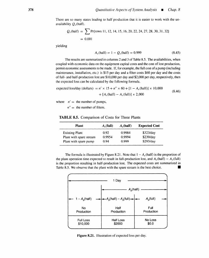
378 Quantitative Aspects ofSystemAnalysis - Chap. 8
There are so many states leading to half production that it is easier to work with the un-availability Q,\. (half).
Qs(half) = LPr{rows II, 12, 14, IS, 16,20,22,24,27,28,30,3I,32}
= 0.001
yielding
As(halt) = I - Qs(half) = 0.999 (8.45)
(8.46)
The results are summarized in columns 2 and 3 of Table8.5. The availabilities,whencoupled with economic data on the equipment capital costs and the cost of lost production,permiteconomicassessments to be made. If, for example, the full cost of a pump (includingmaintenance, installation, etc.) is $15 per day and a filter costs $60 per day and the costsof full- and half-production lost are $10,000 per day and $2,000 per day, respectively, thenthe expected loss can be calculated by the following formula.
expected loss/day (dollars) = n' x IS + n" x 60 + [I - As (half)] x 10,000
+ [As(half) - As(full)] x 2,000
where n' = the number of pumps,
n" = the number of filters.
TABLE 8.5. Comparison of Costs for Three Plants
Plant
Existing PlantPlant with spare streamPlant with spare pump
0.920.99540.94
As(half)
0.99840.99940.999
Expected Cost
$323/day$239/day$293/day
The formula is illustrated by Figure 8.21. Note that 1- A,\' (half) is the proportion ofthe plant operation time expected to result in full-production lost, and As(half) - As (full)is the proportion resulting in half-production lost. The expected costs are summarized inTable 8.5. Weobserve that the plant with the spare stream is the best choice. •
r "'1 Day
As(half)
....-. 1 - As(half) ~~As(half) - As(full) ......~ As(fulI) ~
No Half FullProduction Production Production
Full Loss Half Loss No Loss$10,000 $2000 $0.0
'- ~
Figure 8.21. Illustration of expected loss per day.

Sec. 8.4 • Structure-Function Approach
8.4 STRUCTURE-FUNCTION APPROACH
8.4.1 Structure Functions
379
It is possible to describe the state of the basic event or the system by a binary indicatorvariable. If we assign a binary indicator variable Y; to the basic event i, then
Y; == { 1, when the basic event exists0, when the event does not exist (8.47)
Similarly, the top event is associated with a binary indicator variable 1/J (Y) related tothe state of the system by
(Y)__ { 1, when the top event exists
1/J (8.48)0, when the top event does not exist
Here Y = (Y1, Y2, ... , Yn ) is the vector of basic event states. The function 1/J(Y) is knownas the structure function for the top event.
8.4.2 System Representation
8.4.2.1 Gated AND tree. The top event of the gated AND tree in Figure 8.2 existsif and only if all basic events BI, ... , B; exist. In terms of the system structure function,
n
1/J(Y) == 1/J(YI, Y2, ... , Yn ) == 1\ Y; == YI /\ Y2 /\ ... /\ Yn (8.49);=1
where Y; is an indicator variable for the basic event B;.The structure function can be expressed in terms of algebraic operators (see Table
A.2, appendix of Chapter 3):
n
1/J(Y) == nY; = Y1Y2... Yn;=1
(8.50)
8.4.2.2 Gated OR tree. The gated OR tree of Figure 8.3 fails (the top event exists)if any of the basic events BI, B2, ... , B; exist. The structure function is
n
1/J(Y) == VY; == Y1V Y2 V ... V Yn;=1
and its algebraic form is
n
1/J(Y) == 1 - n[1 - Y;];=1
= 1 - [1 - YIJ[1 - Y2] ... [1 - Yn ]
If the n in Figure 8.3 is two, that is, for a two-event series structure
1/J(Y) = YI V Y2 == 1 - [1 - Y1][1 - Y2]
= Y1 + Y2 - Y1Y2
(8.51)
(8.52)
(8.53)
(8.54)
(8.55)
This result is analogous to (8.20): Here Y1Y2 represent the probability of the intersectingportion of the two events B1 and B2.
380 Quantitative Aspects ofSystem Analysis • Chap. 8
8.4.2.3 Two-out-of-three system. A slightly more sophisticated example is thetwo-out-of-three voting system of Figure 8.8. The structure function is
(8.56)
(8.59)
(8.60)
and its algebraic expression is obtained in the following way:
1/I(Y) == ] - [I - (Y1 1\ Y2)][1 - (Y2 1\ Y3)][1 - (Y3 1\ Y1) ] (8.57)
== I - [I - Y1Y2][1 - Y2Y3][1 - Y3Yt ] (8.58)
This equationcan beexpandedand simplifiedby the absorptionlawof TableA.3, Chapter 3:
1/I(Y) == I - [1 - Y1Y2 - Y2Y3 - Y3Y1 + Y1Y2Y2Y3+ Y2Y3Y3Yt
+ Y3 Yt Yt Y2 - YI Y2 Y2 Y3 Y3 Ytl== YtY2+ Y2Y3+ Y3Yt - 2Y1 Y2Y3
where the absorption law
YtY2Y2 Y3 == Y2 Y3Y3 Yt == Y3YtY1Y2 == YtY2Y2Y3Y3Yt == YtY2Y3 (8.61)
was used in going from (8.59) to (8.60).
8.4.2.4 Tail-gas quench and clean-up system. Structure functionscan be obtainedinastepwise way. Denoteby 1/11 (Y) and 1/12 (Y) the structurefunctionsfor the firstandsecondAND gates of Figure 8.13:
(8.62)
Here, YB is an indicator variable for basic event B, and so on. The structure function forthe fault tree is
1fJ(Y) = YA V 0/1 (Y) V YD v 1fJ2(Y) V YG
== I - [I - YA][l -1/It(Y)][1 - YD][I -1/I2(Y)][1 - YG] (8.63)
== 1 - [I - YA][l - YBYc][l - YD][I - YEYF][l - YG]
8.4.3 Unavailability Calculations
It is of significanceto recognize the probabilisticnature of expressionssuch as (8.55),(8.60), and (8.63). If we examine the system at some point in time, and the state of thebasic event Yi is assumed to be a Bernoulli or zero-one random variable, then 1/1 (Y) is alsoa Bernoulli random variable. The probability of existence of state Yi == 1 is equal to theexpected value of Yi and to the event B, probability.
Pr{Yi == I} == Pr{B i } == E{Yi } (8.64)
(8.65)
(8.66)
(8.67)
Notice that this probabilityis the unavailability Qi (t), orexistenceprobability, dependingonwhether basicevent B, is a component failureor humanerror or environmentalimpact. Theprobabilityof the topevent, that is, the unavailability Qs (t) is the probabilityPr{1/1 (Y) == I},or expectation E {1/1 (Y)}. An alternative way of stating this is as follows:
Qs(t) == Pr{topevent}
== Pr{1/1 (Y) == I} == E {1/1 (Y) }
== L 1/I(Y)Pr{Y}y
The next three examples demonstrate the use of structure functions in system analysis.

Sec. 8.4 • Structure-Function Approach 381
Example 5-Two-out-of-three system. Compare the unavailability for a two-out-of-three votingsystem with that of a two-component series systemfor
(8.68)
Solution: For the two-out-of-three system,accordingto (8.60)
Qs(t) = E{l/J(Y)}
= E{YlY2} + E{Y2Y3 } + E{Y3Yd - 2E{YlY2Y3 } (8.69)
= E{YdE{Y2} + E{Y2}E{Y3 } + E{Y3}E{Ytl- 2E{YtlE{Y2}E{Y3 } (8.70)
= 3 x 0.62- 2 X 0.63 = 0.65 (8.71)
Notethat theexpectationof the productof independentvariables is equal to theproductofexpectationof these variables. This property is used in going from (8.69) to (8.70).
For the series system, from equation (8.55),
Qs(t) = E{l/J(Y)} = E{Y l } + E{Y2} - E{Y t}E{Y2}
= 2 x 0.6 - 0.62 = 0.84
Hence a one-out-of-two system has an 84% chance of being in the top event state, and thetwo-out-of-three systemhas a smaller,64.8% probability. •
Example 6--Tail-gas quench and clean-up system. CalculatethesystemunavailabilityQs (t) for the fault tree of Figure 8.13, assumingcomponentunavailabilities of (8.34).
Solution: Accordingto (8.63) we have
Qs(t) = E{l/J(Y)}
= I - E{[I - YAHI - YBYcHI - YDHI - YEYFHI - YGll(8.72)
Each factor in the expected value operator E of this equation has different indicator variables, andthese factors are independentbecause the indicator variables are assumed to be independent. Thus(8.72) can be written as
Qs(t) = 1 - E{l - YA}E{l - YBYc}E{1 - YD}E{l - YEYF}E{I - YG}
= 1 - [I - E{YA}][I - E{YB}E{Yc}]x [I - E{YD}][I - E{YE}E{YF}][I - E{YG}]
The componentunavailabilities of (8.34) give
Qs(t) = I - [1 - 0.9][1 - (0.8)(0.7)][1 - 0.6][1 - (0.5)(0.4)][1 - 0.3]
= 0.99
(8.73)
(8.74)
(8.75)
This confirmsthe result of (8.35).Contraryto (8.72), each indicatorvariableappearsmorethanonce in theproductsof (8.58), the
structurefunction for a two-out-of-three system. For example, the variable Y2 appears in [I - Yt Y2]and [1- Y2Y3]. Herewe cannotproceedas we did in goingfrom (8.72) to (8.74) becausethesefactorsare no longer independent. This is confirmed by the following derivation, which gives an incorrectresult:
Qs(t) = 1- E{I - YtY2}E{1 - Y2Y3}E{1 - Y3Yd
= I - [I - E{YdE{YdHI - E{Y2}E{Y3}][1 - E{Y3}E{Yl }]
Substituting(8.68) into the above,
This contradicts (8.71).
(8.76)
•
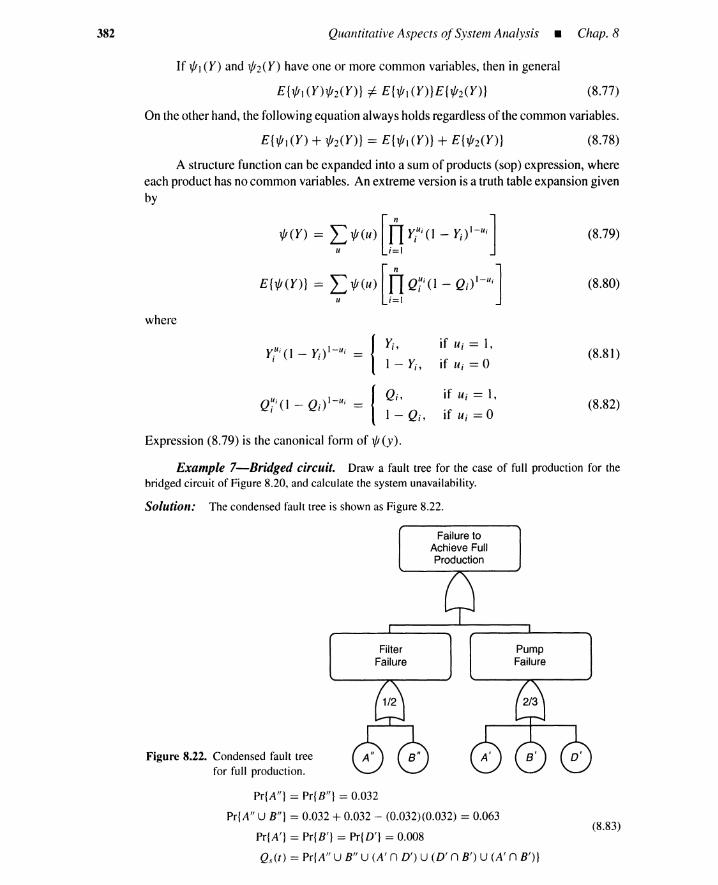
382 Quantitative Aspects ofSystem Analysis _ Chap. 8
If ljJl (Y) and ljJ2(Y) have one or more common variables, then in general
(8.77)
On the other hand, the followingequation alwaysholds regardlessof the common variables.
(8.78)
A structure function can be expanded into a sum of products (sop) expression, whereeach product has no common variables. An extreme version is a truth table expansiongivenby
ljJ(Y) == L ljJ(u) [n yt i (I - y;)I-Ui]u 1=1
E{1{!(Y)} = ~ 1{!(u)[0 Q~i(l - Q;)I-Ui]
where
yt; (I - Yi ) I-u; IYi , if u, == 1,
1 - Yi , if u, == 0
Q7i(1 - Qi)l-u; Io.. if u, == 1,==
l-Qi, if u, == 0
Expression (8.79) is the canonical form of ljJ(y).
(8.79)
(8.80)
(8.81)
(8.82)
Example 7-Bridged circuit. Draw a fault tree for the case of full production for thebridged circuit of Figure 8.20, and calculate the system unavailability.
Solution: The condensed fault tree is shown as Figure 8.22.
Failure toAchieve FullProduction
Figure 8.22. Condensed fault treefor full production.
FilterFailure
PumpFailure
Pr{A"} = Pr{B"} = 0.032
Pr{A" U B"} = 0.032 + 0.032 - (0.032)(0.032) = 0.063
Pr{A'} = Pr{B'} = Pr{D'} = 0.008
Qs(t) = Pr{A" U B" U (A' n D') U (D' n B') U (A' n B')}
(8.83)
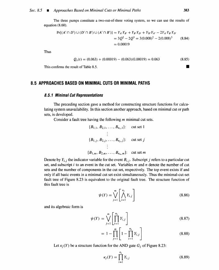
Sec. 8.5 • ApproachesBased on Minimal Cuts or Minimal Paths 383
The three pumps constitute a two-out-of-three voting system, so we can use the results ofequation (8.60).
Pr{(A' n D') U (D' n B') U (A' n B')} = YA,YB, + YB,YD, + YD,YA, - 2YA,YB,YD,
=3Q2 - 2Q3 = 3(0.008)2 - 2(0.008)3 (8.84)
= 0.00019
Thus
Qs(t) = (0.063) + (0.00019) - (0.063)(0.00019) = 0.063
This confirms the result of Table 8.5.
8.5 APPROACHES BASED ON MINIMAL CUTS OR MINIMAL PATHS
8.5.1 Minimal Cut Representations
(8.85)
•
The preceding section gave a method for constructing structure functions for calcu-lating system unavailability. In this section another approach, based on minimal cut or pathsets, is developed.
Consider a fault tree having the following m minimal cut sets.
{Bl,l,B2,1, ... ,Bn 1,1}: cutset!
{B1,m, B2,m, ... , Bnm,m}: cut set m
Denote by Y;,j the indicator variable for the event B;,j. Subscript j refers to a particular cutset, and subscript i to an event in the cut set. Variables m and n denote the number of cutsets and the number of components in the cut set, respectively. The top event exists if andonly if all basic events in a minimal cut set exist simultaneously. Thus the minimal-cut-setfault tree of Figure 8.23 is equivalent to the original fault tree. The structure function ofthis fault tree is
and its algebraic form is
o/(Y) = 2[tJ Yi,j]
= 1-Ii [1 -nYi,j]j=1 ;=1
Let Kj (Y) be a structure function for the AND gate Gj of Figure 8.23:
nj
Kj(Y) == Il Y;,j;=1
(8.86)
(8.87)
(8.88)
(8.89)
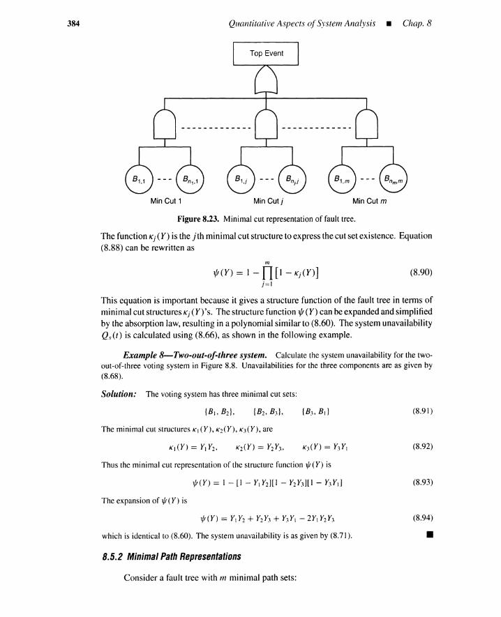
384 Quantitative Aspects ofSystem Analysis - Chap. 8
Min Cut 1 Min Cutj Min Cut m
Figure 8.23. Minimal cut representation of fault tree.
The functionKj(Y) is the jth minimalcut structureto express thecut set existence. Equation(8.88) can be rewritten as
III
l/J(Y) == 1- n[l-Kj(Y)]j=1
(8.90)
This equation is important because it gives a structure function of the fault tree in terms ofminimalcut structuresKj(Y) 'so The structurefunction l/J (Y) can beexpandedand simplifiedby the absorption law,resulting in a polynomialsimilar to (8.60). The system unavailabilityQ.\. (t) is calculated using (8.66), as shown in the following example.
Example 8-Two-out-of-three system. Calculate the system unavailability for the two-out-of-three voting system in Figure 8.8. Unavailabilities for the three components are as given by(8.68).
Solution: The voting system has three minimal cut sets:
(8.91)
The minimal cut structures K)(Y), K2(Y), K3(Y), are
(8.92)
Thus the minimal cut representation of the structure function ljJ(Y) is
The expansion of ljJ (Y) is
which is identical to (8.60). The system unavailability is as given by (8.71).
8.5.2 Minimal Path Representations
Consider a fault tree with In minimal path sets:
(8.93)
(8.94)
•
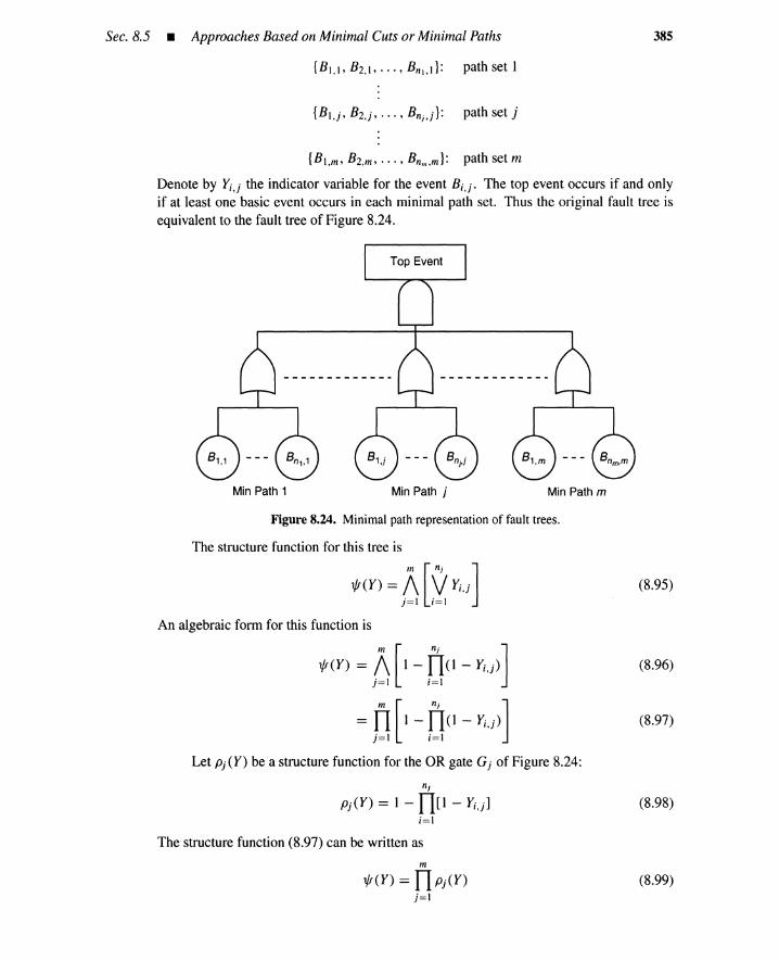
Sec. 8.5 • Approaches Based on Minimal Cuts or Minimal Paths 385
{B l,m, B2,m, ... ,Bnm,m}: path set m
Denote by Yi,j the indicator variable for the event Bi]. The top event occurs if and onlyif at least one basic event occurs in each minimal path set. Thus the original fault tree isequivalent to the fault tree of Figure 8.24.
Min Path 1 Min Path j Min Path m
Figure 8.24. Minimalpath representation of fault trees.
The structure function for this tree is
~(Y) = 6[2 Yi,j]
An algebraic form for this function is
~(Y) = 6[1 -DO -Yi,j)]
=D[1 -00 - Yi,j)]
Let Pj (Y) be a structure function for the OR gate Gj of Figure 8.24:
nj
Pj(Y) == 1 - n[1 - Yi,j];=1
The structure function (8.97) can be written as
m
l/J(Y) == nPj(Y)j=1
(8.95)
(8.96)
(8.97)
(8.98)
(8.99)
386 Quantitative Aspects ofSystem Analysis • Chap. 8
This 1/1 (Y) is a minimal path representation, and the Pi (Y) is the jth minimal path structureto express the existence of path set failure. The minimal path representation 1/I(Y) can beexpanded and simplified via the absorption law. The system unavailability Qs(t) can becalculated by using (8.66), as shown in the next example.
Example 9-Two-out-of-three system. Calculate the system unavailabilityfor the two-out-of-three voting system of Figure 8.8. Unavailabilities for the three components are given by(8.68).
Solution: The voting system has three minimal path sets:
(8.100)
The minimal path structures are
PI (Y) = I - [I - Yd[ I - Y2] = YI + Y2 - YIY2
P2 (Y) = I - [I - Y2][ I - Y3] = Y2+ Y3 - Y2Y3
P3(Y) = I - [I - Y3][1 - Yd = Y3+ YI - Y3YI
The minimal path representation ljJ(Y) is
ljJ(Y) = [YI + Y2 - YIY2][Y2 + Y3 - Y2Y3][Y3+ YI - Y3Yd
Expanding ljJ(Y),
ljJ(Y) = YI Y2 + Y2Y3+ Y3YI - 2YIY2Y3
which is identical to (8.60). The system unavailability is again given by (8.71).
8.5.3 Partial Pivotal Decomposition
(8.101)
(8.102)
(8.103)
•Ifbasic events appear in more than one minimal cut set, factors [1 - Kj(Y)]'S in (8.90)
are no longer independent, and the equality
III
E{1/I(Y)} == 1 - n[I - E{Kj(Y)}]j=l
does not hold. For the same reason, (8.99) does not imply that
III
E{1/I(Y)} == nE{pj(Y)}j=l
(8.104)
(8.105)
One way of calculating E {1/1 (Y)} is to expand 1/1 (Y) and simplify the results by theabsorption law. This is a tedious process, however, when the expansion contains a largenumber of terms. The process can be simplified by partial pivotal decomposition.
The structure function 1/1 (Y) is first rewritten as
(8.106)
where 1/1 (1;, Y) and 1/1 (0;, Y) are binary functions obtained by setting the ith indicatorvariable Y; to unity and zero, respectively. These binary functions can be pivoted aroundother indicator variables until the resulting binary functions consist only of independentfactors; then E {1/1 (Y)} can be easily calculated.
In terms of Boolean operators, equation (8.106) becomes
1/1 (Y) == [Y; /\ 1/1 (1;, Y)] v (r; /\ 1/1 (0;, Y)]
== Y; . 1/1 (true., Y) V Y; . 1/1 (false., Y)
(8.107)
(8.108)
Sec. 8.5 • Approaches Based on Minimal Cuts or Minimal Paths 387
A Boolean AND operation is denoted by symbol /\, which is often replaced by the equivalentmultiplication operation, that is, Y1 /\ Y2 = Y1 • Y2 = Y1Y2. Values 1; and 0; denote trueandfalse values of ith indicator variable Y;, respectively.
These algebraic or Boolean pivotal decomposition techniques are demonstrated bythe following example.
Example 10-Two-out-of-three system.(8.102).
'l/J(Y) = Yt[Y2+ Y3 - Y2Y3]
+ [1 - YtlY2[Y2+ Y3 - Y2Y3]Y3
= Yt[Y2+ Y3 - Y2Y3]
+ [1 - YtlY2Y3
+[I-Yt][I-Y2]·0
Thus
Consider the minimal path representation of
'l/J(Y) = Yt'l/J(I t , Y)
+ [1 - Yd'l/J(Ot, Y)
= Yt'l/J(l t, Y)
+ [1 - YdY2'l/J(Ot, 12, Y)
+ [1 - Ytl [1 - Y2]'l/J (Ot , O2, Y)
(8.109)
Note that Yt and [Y2+ Y3 - Y2Y3] have different indicator variables. Similarly, [1 - Yt], Y2, and Y3have no common variables. Thus each product in (8.109) consists of independent factors, and theexpected value E{'l/J(Y)} is given by
To confirm (8.110), we substitute (8.68)
Qs(t) = E{'l/J(Y)} = (0.6)[0.6 + 0.6 - 0.62] + [1 - 0.6](0.6)2
= 0.65
The results of (8.71) are obtained; thus the methodology is confirmed.A Boolean decomposition yields
ljJ(Y) = YIY2 V Y2Y3 V Y3YI
= Yt (Y2 V Y2Y3 v Y3) V VI (Y2Y3)
= Yt (Y2 v Y3) V VI (Y2Y3)
Because the two terms in the last equation are mutually exclusive, we have
Pr{Yt(Y2 v Y3) = I} = Pr{YtV2V3 = I}
= Qt [1 - (1 - Q2)(I - Q3)]
Pr{V t(Y2Y3) = I} = (1 - Qt)Q2Q3
Pr{'l/J(Y) = I} = Qt[l - (I - Q2)(1 - Q3)] + (I - Qt)Q2Q3
Qs (t) = Pr{'l/J (Y) = I} = (0.6) [I - 0.42] + [I - 0.6] (0.6)2
= 0.65
The results of (8.71) are obtained again.
8.5.4 Inclusion-Exclusion Formula
Define event dj by
dj = all basic events exist in the jth minimal cut set at time t.
(8.110)
(8.111)
(8.112)
(8.113)
(8.114)
(8.115)
(8.116)
(8.117)
(8.118)
(8.119)
•
388 Quantitative Aspects ofSystem Analysis _ Chap. 8
The top event T can be expressed in terms of d, as
m
T == Ud., (In == total number of minimal cuts)j=1
Thus
m Ill-I III
== LPr{dj}- L L Pr{djndk }
.i=1 .i=1 k=j+1
+ ... + (_1),-1
(8.120)
(8.121)
(8.122)
Equation (8.122) is an expansion of (8.121) obtained by the so-called inclusion-exclusion
formula. The rth term on the right-hand side of (8.122) implies the contribution to Qs(r)from r out of III minimal cut sets being simultaneously failed at time t; that is, all the basicevents in these r minimal cut sets exist. A very useful property of (8.122) is that the topevent probability is given in terms of intersections, which are easier to calculate than theunions in (8.121).
For small systems it is relativelyeasy to get exact values for Qs(r), and this is demon-strated by the following example.
Example 11-Two-out-of-three system. Calculate Qs (t) for the two-out-of-three votingsystem of Figure 8.8 by assuming the component unavailabilities of (8.68), using (8.122).
Solution: From the three minimal cut sets of the system, we have
(8.123)
The exact expression for Q.\, (t) from (8.122) is
3 2 3 ] 2 3
Qs(t) = LPr{dj } - L L Pr{dj ndk } + L L L Pr{dj ndk nd,}j =] j =) k=j + ) j =] k= j +) I=k +)
= Pr{d]} + Pr{(h} + Pr{d3 }
- [Pr{d) n {hI + Pr{d] n d3 } + Pr{d2 n d3 }] + Pr{d] n d: n d3 }
[A] == [Pr{dd + Pr{(h} + Pr{d3 }] = Q2 + Q2 + Q2 = 1.08
[B] == [Pr{d] n d2 } + Pr{d) n d3 } + Pr{d2 n d3 }] = Q3 + Q3 + Q3 = 0.65
[C] == Pr{d] n d: n d3 } = Q3 = 0.22
Thus
Qs(t) = [A] - [B] + [C] = 0.65
This confirms (8.71).
(8.124)
(8.125)
(8.126)
•
Sec. 8.6 • Lower and Upper Boundsfor System Unavailability
We note here an expression of Qs(t) in terms of coverage a(Y) of cut sets.
m
a(Y) == L Kj(Y)j=l
389
(8.127)
(8.128)m
Qs(t) == L L[I/a(Y)]Kj(Y)Pr{Y}Y,a(Y)2:1 j=l
This is called a coverageformula for Qs(t). Function a denotes how many cut sets exist atstate vector Y.
8.6 LOWER AND UPPER BOUNDS FOR SYSTEM UNAVAILABILITY
For a large, complicated fault tree, exact system unavailability calculation by the methodsof the preceding sections are time consuming. When computing time becomes a factor,unavailability lower and upper bounds can be calculated by the short-cut methods in thissection.
8.6.1 Inclusion-Exclusion Bounds
Equation (8.122) can be bracketed by
m m-l m m
LPr{dj} - L L Pr{dj ndk} S Qs(t) ~ LPr{dj}j=l j=l k=j+l j=l
(8.129)
Example 12-Two-out-of-three system. For Example 11 in the preceding section wehave
Qs(t)min = [A] - [B] = 0.43
Qs(t)max = [A] = 1.08
The exact value of Qs (r) is 0.65, so these lower and upper bounds are approximate. However, thebrackets are normally within three significant figures of one another because component unavailabil-ities are usually much less than 1. •
Example 13-Two-out-of-three system. Calculate Qs(t), Qs(t)min, and Qs(t)max byassuming Q = 0.001 in Example 12.
Solution: From (8.125)
[A] = Q2 + Q2 + Q2 = 3.0 X 10⁻⁶
[B] = Q3 + Q3 + Q3 = 3.0 X 10⁻⁹
[C] = Q3 = 1.0 X 10⁻⁹
Thus
Qs(t) = [A] - [B] + [C] = 2.998 X 10⁻⁶
Qs(t)min = [A] - [B] = 2.997 x 10- 6
Qs(t)max = [A] = 3.0 x 10⁻⁶
We have tight lower and upper bounds. •In general, the formula gives a lower bound when r is even; the formula yields an
upper bound when r is odd.

(8.130)
390 Quantitative Aspects ofSystem Analysis - Chap. 8
8.6.2 Esary and Proschan Bounds
We now restrict our attention to structure functions that are coherent (monotonic).The engineering interpretation of this is that, in a coherent system, the occurrence of acomponent failure always results in system degradation. Formally, l/J(Y) is coherent if [3]:
1. l/J(Y) == 1 if Y == (1,1, ,1)
2. l/J(Y) == 0 if Y == (0,0, ,0)
3. l/J(Y) ~ l/J(X) if Yi ~ Xi for all i == 1, ... , n
4. each basic event appears in at least one minimal cut set
For a coherent structure function, the right-hand sides of (8.104) and (8.105) giveupper and lower bounds for the system unavailability Q.\,(t) [4]:
m(p) m(c)nE{pj(Y)} ::s Qs(t) ::s I-n[1 -E{Kj(Y)}]j=l j=1
where mt p) and mic) are total numbers of minimal path sets and cut sets, respectively.
Example 14-Two-out-of-three system. Calculate Esary and Proschan bounds for theproblem in Example 13 of the preceding section.
Solution:
KI = Y1Y2, K2 = Y2Y3,
p) = Y1 + Y2 - Y1Y2
P2 = Y2 + Y3 - Y2 Y3
P3 = Y3 + Y1 - Y3 Y1
Because E{Y)} = E{Y2} = E{Y3 } = Q = 0.001, we have
Qs(t)min = [Q + Q - Q2]3 = 8.0 X 10- 9
Qs(t)max = I - [I - Q2]3 = 3.0 X 10- 6(8.131)
The upper bound is as good as that obtained by bracketing, while the lower bound is extremelyconservativee •
8.6.3 Partial Minimal Cut Sets and Path Sets
Pick up In (c)' minimal cut sets and nz(p)' minimal path sets. Here m(c)' and m(p)'
are less than the actual number of minimal cut sets m(c) and path sets m(p), respectively.The structure function l/JL (Y) with these In (c)' cut sets is
m(c)'
l/JL(Y) == 1 - n[1 - Kj(Y)]j=1
(8.132)
(8.133)
where Kj(Y) is the jth minimal cut structure. Similarly, the structure function l/Ju (Y) withthe In (p)' path sets is
m(p)'
l/Ju(Y) == n Pj(Y)j=1
Because the structure function l/JL (Y) has fewer minimal cut sets than l/J (Y), we have
(8.134)
Sec. 8.7 • System Quantification by KIT[
Similarly,
1/Iu (Y) 2: 1/1 (Y)
Thus
E {1/1L (Y)} :::: E {1/1 (Y)} :::: E {1/Iu (Y)}
or
391
(8.135)
(8.136)
(8.137)
Example IS-Tail-gas quench and clean-up system. Calculate Qs(t)min, Qs(t), andQs (t)max for the fault tree of Figure 8.13. Assume the component unavailabilities at time t to be0.001.
Solution: The fault tree has five minimalcut sets,
fA}, fD}, fG}, fB, C}, fE, F}
and four minimalpath sets:
fA, D, G, C, F}, fA, D, G, C, E}, fA, D, G, B, F}, fA, D, G, B, E}
(8.138)
(8.139)
(8.142)
(8.143)
(8.140)
(8.141)
Take only the cut sets fA}, fD}, and fG} (ignore the higher-order ones) and only two path setsfA, D, G, C, F} and fA, D, G, B, E}. Then,
1/J(Y) = 1 - [I - YAHI - YDHI - YGHI - YBYcHI - YEYF ]
1/JL(Y) = I - [1 - YAHI - YDHI - YG]
1/Ju(Y) = [1 - (1 - YA)(I - YD)(I - YG)(I - Yc )( 1 - YF ) ]
x [1 - (1 - YA)(I - YD)(1 - YG)(I - YB)(I - YE)]
= 1 - (1 - YA)(I - YD)(I - YG)( 1 - YB)(I - YE)
- (1 - YA)( 1 - YD)(I - YG)(I - Yc)(1 - YF )
+ (I - YA)( 1 - YD)(I - YG)( 1 - YB)( 1 - YE)( 1 - Yc )( 1 - YF )
Thus
Qs(t) = 1 - (0.999)3(0.999999)2 = 2.999 X 10- 3
Qs (t)min = 1 - (0.999)3 = 2.997 x 10⁻³
Qs(t)max = 1 - (0.999)5 - (0.999)5 + (0.999)7 = 3.001 X 10⁻³
Good upper and lowerboundsare obtained.
(8.144)
•As a first approximation, it is reasonable to include only the one- or two-event minimal
cut sets in the m(c)' cut sets. Similarly, we take as the m(p)' path sets, minimal path setscontaining the fewest number of basic events. Because fewer cut sets and path sets areinvolved, the calculation can be simplified. Further simplifications are possible if we pick outnearly disjoint cut sets or path sets because the structure functions 1/Iu (Y) and 1/1L (Y) can beexpanded into polynomials with fewer terms, each of which consists of independent factors.
8.7 SYSTEM QUANTIFICATION BY KITT
The previous sections covered availability and unavailability quantification methods forrelatively simple systems. This section develops the theory and techniques germane toobtaining unavailabilities, availabilities, expected number of failures and repairs, and con-ditional failure and repair intensities, starting with minimal cut sets or path sets of large

392 Quantitative Aspects ofSystem Analysis _ Chap. 8
and complicated fault trees. We discuss, in some detail, the KITT (kinetic tree theory), andshow how system parameters can be guesstimated by approximation techniques based oninclusion-exclusion formulae. To be consistent with previous chapters, we present here arevised version of Vesely's original derivation [5]. A KITT improvement is described inreference [6]. Other computer codes are surveyed in IAEA-TECDOC- 553 [7].
8.7.1 Overview ofKITT
The code is an application of kinetic tree theory and will handle independent basicevents that are nonrepairable or repairable, provided they have constant failure rates andconstant repair rates. However, the exponential failure and/or repair distribution limitationcan be circumvented by using the "phased mission" version of the program (KITT-2), whichallows for tabular input of time-varying failure and repair rates. KITT also requires as inputthe minimal cut sets or the minimal path sets. Inhibit gates are permitted.
Exact, time-dependent reliability parameters are determined for each basic event andcut set, but for the system as a whole the parameters are obtained by upper- or lower-boundapproximations, or by bracketing. The upper and lower bounds are generally excellentapproximations to the exact parameters. In the bracketing procedure the various upper andlower bounds can be obtained as close to each other as desired, and thus exact values forsystem parameters are obtained if the user so chooses.
The probability characteristics, their definitions, the nomenclature, and the expected(mostly asymptotic) behavior of the variables are summarized in Tables 8.6 and 8.7. A flowsheet of the KITT computation is given as Figure 8.25. The numbers on the flow sheetrepresent the equations in Table 8.8 used to obtain the parameters.
TABLE 8.6. System Parameters Calculated by KITT
Symbols
Cut KITTComponent Set System Symbol Definition Name
Q(t) Q*(t) Qs(t) Q Probabilityof a failed state Unavailabilityat time t
w(t) w*(t) ws(t) W Expected numberof failures Unconditionalper unit time at time t failure intensity
v(t) v* (t) Vs (t) V Expectednumber of repairs Unconditionalper unit time at time t repair intensity
)..(t) )..*(t) )..s(t) L Probabilityof a failure Conditionalper unit time at time t, failure intensitygiven no failures at time t
J-l(t) J-l*(t) J-ls(t) M Probabilityof a repair Conditionalper unit time at time t, repair intensitygiven no repairs at time t
W(O, t) W*(O, t) W\·(O, t) WSUM Expected number of Expected numberfailures in time interval [0, t) of failures
V (0, t) V*(O, t) Vs(O, t) VSUM Expected number of Expected numberrepairs in time interval [0, t) of repairs
F(t) F*(t) Fs(t) Not Probabilityof one or more UnreliabilityAvailable failures in time interval [0, t)

Sec. 8.7 • System Quantification by K/TT
TABLE 8.7. Behavior of System Parameters with Constant Rates A and J.L
Component Level
Parameter Repairable Nonrepairable
Q(t) Constant Q(t) after t > 3MTTR, Q(t) --+ 1 as t --+ 00,
Q(t) « 1 Q(t) = F(t) = W(O, t) = 1 - e-At
wet) Constant wet) after t > 3MTTR, wet) decreaseswith time,w(t) :::: A w(t) = !(t) = Ae-At
A(t) Constant A. ConstantAA:::: wet) after t > 3 MTTR
W(O, t) W (0, t) --+ 00 as t --+ 00 W (0, t) --+ 1 as t --+ 00,
W(O, t) = F(t) = Q(t)
F(t) F (r) --+ 1 as t --+ 00 F (t) --+ 1 as t --+ 00,
F(t) = W(O, t) = Q(t)
Cut Set Level
Parameter Repairable Nonrepairable
Q*(t) Constant Q*(t) after t > 3MTTR, Q*(t) --+ 1 as t --+ 00,
Q*(t) « 1 Q*(t) = F*(t) = W*(O, t)
w*(t) Constant w*(t) after t > 3MTTR, w* (r) increases, then decreaseswithw*(t) :::: A"(r) time, w*(t) = f*(t)
A*(t) ConstantA*(t) after t > 3MTTR, A*(t) increaseswith timeA*(t) :::: w*(t)
W*(O, t) W*(O, t) --+ 00 as t --+ 00 W*(O, t) --+ 1 as t --+ 00,
W*(O, t) = F*(t) = Q*(t)
F*(t) F*(t) --+ 1 as t --+ 00 F *(r) --+ 1 as t --+ 00,
F*(t) = W*(O, t) = Q*(t)
System Level
Parameter Repairable Nonrepairable
Qs(t) Constant Qs(t) after t > 3MTTR, Qs(t) --+ 1as t --+ 00,
Qs(t) « 1 Qs(t) = Fs(t) = Ws(O, t)
ws(t) Constant ws(t) after t > 3MTTR, ws(t) increases,then decreaseswithws(t) :::: As(t) time, ws(t) = !s(t)
As(t) Constant As(t) after t > 3MTTR, As(t) increaseswith timeAs(t) :::: ws(t)
Ws(O, t) Ws(0, t) --+ 00 as t --+ 00 Ws(0, t) --+ 1 as t --+ 00,
Ws(O, t) = Fs(t) = Qs(t)
Fs(t) F, (t) --+ 1 as t --+ 00 F,(t) --+ 1 as t --+ 00,
Fs(t) = Ws(O, t) = Qs(t)
393
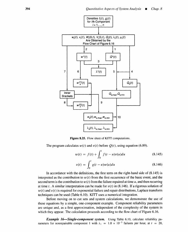
394 Quantitative Aspects ofSystem Analysis _ Chap. 8
Densities f;(t), g;(t)for ith Component
;= 1, ... , n
w;(t), v;(t), W;(O,t), V;(O,t), O;(t), A;(t), Jl;(t)Are Obtained by the
Flow Chart of Figure 6.16
7 6
9
5 ....-----44
°s,max,Os,min
10
Figure 8.25. Flowsheet of KITT computations.
The program calculates w(t) and v(t) before Q(t), using equation (6.89).
w(t) = f(t) +11
f(t - u)v(u)du (8.145)
u(r) =11
g(t - u)w(u)du (8.146)
In accordance with the definitions, the first term on the right-hand side of (8.145) isinterpreted as the contribution to wet) from the first occurrence of the basic event, and thesecond term is the contributionto w(t) from the failure repairedat time u, and then recurringat time t. A similar interpretationcan be made for v(t) in (8.146). If a rigorous solution ofw(t) and v(t) is required for exponential failure and repair distributions,Laplace transformtechniques can be used (Table6.10). KITT uses a numerical integration.
Before moving on to cut sets and system calculations, we demonstrate the use ofthese equations by a simple, one-component example. Component reliability parametersare unique and, as a first approximation, independent of the complexity of the system inwhich they appear. The calculation proceeds according to the flow chart of Figure 6.16.
Example 16-Single-component system. Using Table 6.10, calculate reliability pa-rameters for nonrepairable component 1 with AI = 1.0 x 10- 3 failures per hour, at t = 20,
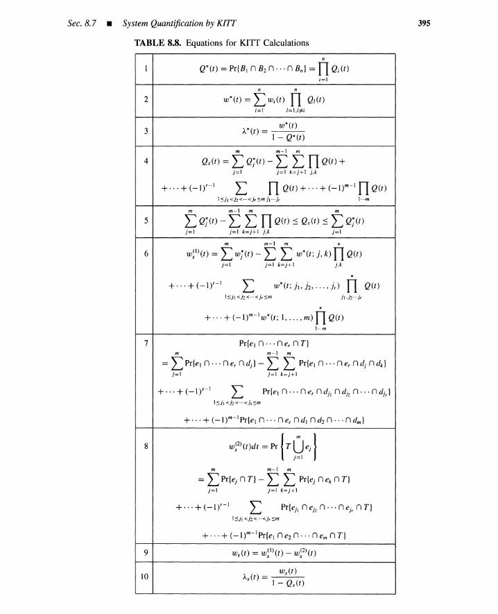
Sec. 8.7 • System Quantification by K/1T
TABLE 8.8. Equations for KITT Calculations
n
Q*(t) = Pr{B 1n B2 n··· n Bn } =nQ;(t);=1
395
2
3
4
n n
w*(t) = L w;(t) n Ql(t);=1 1=1.Ii=;
* w*(t)A (r) -
- 1 - Q*(t)
m m-l m
as» = L Qj(t) - L L nQ(t) +j=1 j=1 k=j+l j.k
+ ... + (_1)'-1 L no» + ... + (_I)m-l nQ(t)
l~h <h<···<jr~mh···jr 1···m
m m-l m m
5 L Qj(t) - L L nQ(t) ~ Qs(t) ~ L Qj(t)j=1 j=1 k=j+l j.k j=1
m m-l m *
6 w~1)(t) = L wj(t) - L L w*(t; j, k) nQ(t)j=1 j=1 k=j+l jk
*+ ... +(-1)'-1 L W*(t;jl,j2,· .. .L) n Q(t)
l~h <h<···<jr~m is.h-:»
*+ ... + (_I)m-l W*(t; 1, ... , m) nQ(t)
1..-m
7 Pr{el n ... n e, n T}m m-l m
= L Pr{el n ... n e, n dj} - L L Pr{el n ... n e, n dj n dk}j=l j=1 k=j+l
+... + (_Iy-l
8 w~2)(t)dt = PrITQejIm m-l m
= LPr{ej n T} - L L Pr{ej nek n T}j=1 j=1 k=j+l
+···+(-1)'-1
9
10ws(t)
As(t) = -I---Q-s(-t)

396 Quantitative Aspects ofSystem Analysis _ Chap. 8
t = 500, and t = 1100 hr. Repeat the calculations, assuming that the component is repairablewith MTTR = I/Jll = 10 hr.
Solution: For the nonrepairablecomponent
wet) = Ae-A' , v(t) = 0
Q(t) = l' [w(u) - v(u)]du = I - e-J..' = F(t)o
W(O, t) = l' w(u)du = I - e-J..' = F(t)o
V(O, t) = l' v(u)du = 0o
For the repairable case
AJl A2
-(A+J.L)'wet) = -- + --e
A+Jl A+Jl
vet) = ~[I - e-(A+J.L)']
A+Jl
l ' AQ(t) = [w(u) - v(u)]du = --[I - e-(A+J.L)']
o A+Jl
l ' A ' A2W(O, t) = w(u)du = _/1_ t + [I - e-(A+J.L)']
o A+Jl (A+Jl)2
l ' A AV(O, t) = v(u)du = _Jl_ t - Jl [I _ e-(A+J.L)']
o A+ Jl (A+ Jl)2
The values of Q(t), w(t), and Wen, t) are listed in Table 8.9.
TABLE 8.9. Results of Example 16
Nonrepairable Component, MTTR. =00
t w(t) Q(t) W(O, t) V(O, t)
20 9.80 X 10- 4 1.98 X 10- 2 1.98 X 10- 2 0.0500 6.06 X 10- 4 3.93 X 10- 1 3.93 X 10- 1 0.0
1100 3.33 x 10- 4 6.32 X 10- 1 6.32 X 10- 1 0.0
Repairable Component, MTTR. = 10
t w(t) Q(t) W(O, t) V (0, t)
20 9.91 X 10- 4 8.59 X 10- 3 1.99 x 10- 2 1.13 X 10- 2
500 9.90 x 10--4 9.90 X 10- 3 4.95 X 10- 1 4.85 X 10- 1
1100 9.90 x 10- 4 9.90 X 10- 3 1.09 x 10+0 1.08 x 10+0
Failure Rate AI = 0.001
(8.147)
(8.148)
(8.149)
(8.150)
(8.151)
(8.152)
(8.153)
(8.154)
(8.155)
At t = 1100, 63.2% of the steady-state unavailability Q(00) is attained for the nonrepairablecase, which is consistent with a mean time to failure of 1000 hr. Further,parameter W(O, t) coincideswith unreliability or unavailability Q(t). For the repairable case, steady state is generally reached in
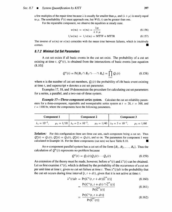
Sec. 8.7 • System Quantification by KIIT 397
a few multiplesof the repair time becauseAis usually far smaller than u, and (A + Jl) is nearlyequalto u, The unreliability F(t) must approachone, but W(O, t) can be greater than one.
For the repairablecomponent,we observe the equalitiesat steady state.
AJlw(oo) = v(oo) = --
A+Jl
l/w(oo) = l/v(oo) = MTTF+ MTTR
(8.156)
(8.157)
The inverse of w (00) or v( 00) coincides with the mean time between failures, which is intuitivelycorrect. •
8.7.2 Minimal Cut Set Parameters
A cut set exists if all basic events in the cut set exist. The probability of a cut setexisting at time t, Q*(t), is obtained from the intersections of basic events [see equation(8.10)]
n
Q*(t) == Pr{Bl n B2 n··· n Bn } == nQ;(t);=1
(8.158)
where n is the number of cut set members, Q;(t) the probability of ith basic event existingat time t, and superscript *denotes a cut set parameter.
Examples 17, 18, and 19 demonstrate the procedure for calculating cut set parametersfor a series, a parallel, and a two-out-of-three system.
Example 17-Three-component series system. Calculatethe cut set reliability param-eters for a three-component, repairable and nonrepairable series system at t = 20, t = 500, andt = 1100hr, where the componentshave the following parameters.
Component 1 Component 2 Component 3
Jl3 = 1/60
Solution: For this configuration there are three cut sets, each component being a cut set. ThusQi(t) = QI (t), Q;(t) = Q2(t), Q3(t) = Q3(t), and so on. The parameters for component 1 werecalculatedin Example 16. For the three components(cut sets) we haveTable8.10. •
An n-component parallel system has a cut set of the form {BI, B2, ... , Bn }. Thus thecalculation of Q* (r) represents no problem because
(8.159)
(8.161)
(8.162)
An extension of the theory must be made, however, before w* (t) and A*(t) can be obtained.Let us first examine A*(t), which is defined by the probability of the occurrence of a cut setper unit time at time t, given no cut set failure at time t. Thus A*(t)dt is the probability thatthe cut set occurs during time interval [t, t +dt), given that it is not active at time t:
A* (t )d t == Pr{C*(t, t +d t ) IC* (t )} (8.160)
Pr{C* (t , t +dt) nC* (t )}-*Pr{C (t)}
Pr{C*(t , t + d t )}
Pr{C* (t)}
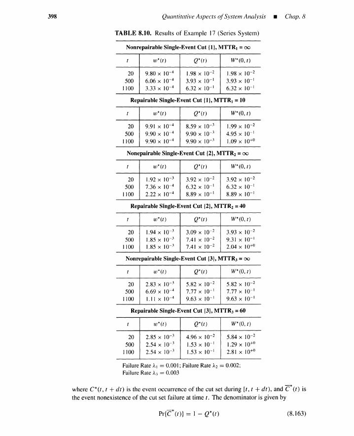
398 Quantitative Aspects ofSystem Analysis • Chap. 8
TABLE 8.10. Results of Example 17 (Series System)
Nonrepairable Single-Event Cut {I}, MTTR. = 00
t w*(t) Q*(t) W* (0, t)
20 9.80 x 10- 4 1.98 X 10- 2 1.98 x 10- 2
500 6.06 X 10- 4 3.93 X 10- 1 3.93 X 10- 1
1100 3.33 x 10⁻⁴ 6.32 X 10- 1 6.32 X 10- 1
Repairable Single-Event Cut {I}, MTTR. = 10
t w*(t) Q*(t) W*(O, t)
20 9.91 x 10- 4 8.59 X 10- 3 1.99 x 10- 2
500 9.90 X 10- 4 9.90 X 10- 3 4.95 X 10- 1
1100 9.90 x 10⁻⁴ 9.90 X 10- 3 1.09 x 10+0
Nonepairable Single-Event Cut {2},MTTR2 = 00
t w*(t) Q*(t) W*(O, t)
20 1.92 x 10- 3 3.92 X 10- 2 3.92 X 10- 2
500 7.36 x 10- 4 6.32 X 10- 1 6.32 X 10- 1
1100 2.22 x 10- 4 8.89 X 10- 1 8.89 X 10- 1
Repairable Single-Event Cut {2},MTTR2 =40
t w*(t) Q*(t) W*(O, t)
20 1.94 x 10- 3 3.09 X 10- 2 3.93 X 10⁻²
500 1.85 x 10- 3 7.41 X 10- 2 9.31 X 10- 1
1100 1.85 x 10- 3 7.41 X 10- 2 2.04 x 10+0
Nonrepairable Single-Event Cut {3}, MTTR3 = 00
t w*(t) Q*(t) W*(O, t)
20 2.83 x 10- 3 5.82 X 10- 2 5.82 X 10- 2
500 6.69 X 10⁻⁴ 7.77 X 10- 1 7.77 X 10- 1
1100 1.11 x 10⁻⁴ 9.63 X 10- 1 9.63 X 10- 1
Repairable Single-Event Cut {3},MTTR3 = 60
t w*(t) Q*(t) W*(O, t)
20 2.85 x 10- 3 4.96 X 10- 2 5.84 X 10- 2
500 2.54 X 10- 3 1.53 X 10- 1 1.29 x 10+0
1100 2.54 x 10- 3 1.53 X 10- 1 2.81 x 10+0
Failure Rate Al = 0.001; Failure Rate A2 = 0.002;Failure Rate A3 = 0.003
where C*(I, 1 + dt) is the event occurrence of the cut set during [1,1 + dt), and C*(I) isthe event nonexistence of the cut set failure at time I. The denominator is given by
Pr{C* (I)} == 1 - Q*(I ) (8.163)

Sec. 8.7 • System Quantification by KI1T 399
Consider the numerator of (8.162). The cut set failure occurs if and only if one of thebasic events in the cut set does not exist at t and then occurs during [t, t +dt), and all otherbasic events exist at t. Thus
n
Pr{C'tt , t + dt)} == L Pr{event i occurs during [t, t + dt), andi=l
the other events exist at t}
Because the basic events are mutually independent,n
Pr{C*(t, t + dt)} == LPr{event i occurs during [t, t +dt)};=1
x Pr{the other events exist at t}n n
== L w;(t)dt n os»;=1 l=l,l¥=;
Consequently, (8.162) can be writtenn n
L w;(t)dt n Ql(t)
'A*(t)dt == i=l l=l,l¥=i1 - Q*(t)
(8.164)
(8.165)
(8.166)
(8.167)
(8.168)
The denominator on the right-hand side of (8.167) represents the probability of thenonexistence of the cut set failure at time t. Each term of the summation is the probabilityof the ith basic event during [t, t +dt) with the remaining basic events already existing attime t. At most, one basic event occurs during the small time interval [t, t + dt), and theterms describing the probability of two or more basic events can be neglected.
The expected number of times the cut set occurs per unit time at time t, that is, w*(t),
is equal to the numerator of (8.167) divided by dt, and given byn n
w*(t) == L w;(t) n Ql(t);=1 l=l,l¥=i
Thus 'A*(t) in (8.167) is calculated from w*(t) and Q*(t):
w*(t)'A*(t) == (8.169)
1 - Q*(t)
Similar equations hold for j1,*(t) and v*(t), that is, v*(t) can be calculated by
and j1,*(t) is given by
n n
v*(t) == L v;(t) n Ql(t);=1 l=l,l¥=i
(8.170)
* v* (t)JL (t) = Q*(t) (8.171)
The integral values W*(O, t) and V*(O, t) are, as before, obtained from the differen-tials w*(t) and v*(t):
W*(O, t) = 1/ w*(u)du
V*(O, t) = 1/ v*(u)du
(8.172)
(8.173)

400 Quantitative Aspects ofSystem Analysis • Chap. 8
Theseequationsare applied inExample 18toa simpleparallelsystem,and inExample19 to a two-out-of-three voting configuration.
Example 18-Two-component parallel system. Calculate the cut set parameters for arepairable and nonrepairable parallel system consisting of components I and 2 of Example 17 att = 20, 500, and 1100.
Solution: Applying (8.158) to the two-component cut set {I, 2} we have
Q*(t) = Q](t)Q2(t)
For the repairablecase, at 20 hr
Q*(t) = (8.59 x 10⁻³)(3.09 x 10- 2) = 2.65 X 10⁻⁴
(8.174)
(8.175)
(8.176)
From (8.168), w*(t) = w) (t)Q2(t) + W2(t)Q] (r); thus for the repairablecase, at 20 hr,
w*(t) = (9.91 x 10⁻⁴)(3.09 x 10⁻² ) + (1.94 x 10⁻³)(8.59 x 10⁻³ )
= 4.73 X 10⁻⁵
From (8.169), A*(t) = w*(t)/[I - Q*(t)]. At 20 hr, for the repairablecase,
4.73 x 10⁻⁵
A*(t) = = 4.73 X 10⁻⁵ (8.177)I - 2.65 X 10⁻⁴
Other differentials v* (z) and J.L *(t) are calculated by (8.170) and (8.171). The integral parametersW*(O, t) and V*(O, t) are readily obtained by equations (8.172) and (8.173). Part of the final resultsare listed in Table8.11.
TABLE 8.11. Results of Example 18
Nonrepairable System
t w*(t) Q*(t) W*(O, t) A*(t)
20 7.65 X 10⁻⁵ 7.76 X 10⁻⁴ 7.73 X 10⁻⁴ 7.65 X 10⁻⁵
500 6.73 X 10⁻⁴ 2.49 X 10-) 2.49 X 10-] 8.96 X 10⁻⁴
1100 4.44 x 10⁻⁴ 5.93 X 10-) 5.93 X 10-] 1.09 X 10- 3
Repairable System
t w*(t) Q*(t) W*(O, t) A*(t)
20 4.73 X 10- 5 2.65 X 10⁻⁴ 5.78 x 10- 4 4.73 X 10⁻⁵
500 9.17xI0-5 7.33 X 10⁻⁴ 4.30 X 10- 2 9.17 X 10⁻⁵
1100 9.17 x 10⁻⁵ 7.33 X 10⁻⁴ 9.80 X 10⁻² 9.17x 10⁻⁵
As expected, the parallel (redundant)configuration is more reliable than the single-componentsystemof Example 16. For the nonrepairablecase, Q* (r) equals W* (0, t) and, for the repairablecase,A*(t) ::::: w*(t) because Q*(t) « 1. •
Example 19-Two-out-of-three system. Calculatethecut set parametersfor a repairableand nonrepairable two-out-of-three votingsystemconsistingof the three componentsof Example 17at t = 20, 500, and 1100 hr.
Solution: The fault tree for this system is given in Figure 8.8, and the cut sets are easily identifiedas K] = {I, 2}, K2 = {2,3}, K3 = {3, I}. Reliabilityparametersfor K] are obtained in Example 18.Parameters for the three cut sets are listed in Table8.12.

Sec. 8.7 • System Quantification by KITI
TABLE 8.12. Results of Example 19 (Two-out-of-Three System)
Nonrepairable System K.(I, 2)
t w*(t) Q*(t) W*(O, t) A*(t)
20 7.65 X 10⁻⁵ 7.76 X 10⁻⁴ 7.73 X 10⁻⁴ 7.65 X 10⁻⁵
500 6.73 X 10⁻⁴ 2.49 X 10- 1 2.49 X 10- 1 8.96 X 10⁻⁴
1100 4.44 x 10⁻⁴ 5.93 X 10- 1 5.93 X 10- 1 1.09 X 10⁻³
Repairable System K.(I, 2)
t w*(t) Q*(t) W*(O, t) A*(t)
20 4.73 X 10⁻⁵ 2.65 X 10⁻⁴ 5.78 X 10⁻⁴ 4.73 X 10⁻⁵
500 9.17 X 10⁻⁵ 7.33 X 10⁻⁴ 4.30 X 10⁻² 9.17x 10⁻⁵
1100 9.17 x 10⁻⁵ 7.33 X 10⁻⁴ 9.80 X 10⁻² 9.17 X 10⁻⁵
Nonrepairable System K2(2, 3)
t w*(t) Q*(t) W*(O, t) A*(t)
20 2.23 X 10⁻⁴ 2.28 X 10⁻³ 2.27 X 10⁻³ 2.23 X 10⁻⁴
500 9.95 X 10⁻⁴ 4.91 X 10- 1 4.91 X 10- 1 1.95 x 10⁻³
1100 3.12 x 10⁻⁴ 8.56 X 10- 1 8.56 X 10- 1 2.17 X 10⁻³
Repairable System K2(2, 3)
t w*(t) Q*(t) W*(O, t) A*(t)
20 1.84 X 10⁻⁴ 1.53 X 10⁻³ 1.97 X 10⁻³ 1.85 x 10⁻⁴
500 4.71 X 10⁻⁴ 1.13 X 10⁻² 2.15 X 10- 1 4.76 X 10⁻⁴
1100 4.71 x 10⁻⁴ 1.13 X 10⁻² 4.98 X 10- 1 4.76 X 10⁻⁴
Nonrepairable System K3(3, 1)
t w*(t) Q*(t) W*(O, t) A*(t)
20 1.13 X 10⁻⁴ 1.15 x 10⁻³ 1.48 x 10⁻³ 1.13 X 10⁻⁴
500 7.35 X 10⁻⁴ 3.06 X 10- 1 3.06 X 10- 1 1.06 x 10⁻³
1100 3.94 x 10⁻⁴ 6.43 X 10- 1 6.42 X 10- 1 1.10 X 10⁻³
Repairable System K3(3, 1)
t w*(t) Q*(t) W*(O, t) A*(t)
20 7.37 X 10⁻⁵ 4.26 X 10⁻⁴ 8.23 X 10⁻⁴ 7.37 X 10⁻⁵
500 1.76 X 10⁻⁴ 1.51 X 10⁻³ 8.03 X 10⁻² 1.76 x 10⁻⁴
1100 1.76 x 10⁻⁴ 1.51 X 10⁻³ 1.86 X 10- 1 1.76 X 10⁻⁴
401
These resultscontainno surprises. The meantime to failure for the components is MTTF3 <
MTTF2 < MTTF1; thus we wouldexpect Qr(t) < Qj(t) < Qi(t) for the nonrepairable case, andthatresultis confirmed at 1100hr:* 0.593 < 0.643 < 0.856. For the repairable case,we alsosee that
*Suffix j attached to the cut set parameters refers to the jth cut set. Cut set 1 = {I, 2}, cut set 2 = {2, 3},cut set 3 = {3, I}.

402 Quantitative Aspects ofSystem Analysis • Chap. 8
Qr(t) < Q;(t) < Q;(t); 7.33 x 10- 4 < l.SI X 10-J < l.13 X 10- 2 because of the shorter repairtimes for the more reliable components.
Another point to note is that a system composed of components having constant failure ratesor constant conditional failure intensities A will not necessarily have a constant conditional failureintensity A* on a cut set level. We see also that, unlike for a nonrepairable component where wet)
decreases with time, w* (r ) increases briefly, and then decreases. •
The KITT program accepts as input path sets as well as cut sets, the calculations beingdone in much the same way. We do not discuss this option.
8.7.3 System Unavailability Qs(t)
As in Section 8.5.4, we define event dj as
dj = all basic events exist in the jth minimal cut set at time t
= the jth minimal cut set failure exists at time t,
The expansion (8.122) in Section 8.5.4 was obtained by the inclusion-exclusion formula,The rth term on the right-hand side of (8.122) is the contribution to Qs (z) from r minimalcut set failures existing simultaneously at time t. Thus (8.122) can be rewritten as
m Ill-I m
Qs(t) == L Qj(t) - L L nQ(t)j=1 j=1 k=j+1 j.k
+ ... + (-I)r-I L n Q(t)
l:s;jl <h< ..<i-sm iv-],
+···+(-I)m-I nQ(t)
I···m
(8.178)
where njl ..-jr is the product of Q(t)'s for the basic events in cut set i.. or j2, ... , or jr.The lower and upper bounds of (8.129) can be rewritten as
m m-I m m
L Q.i(t) - L L Il Q(t) ~ o;« ~ L Qj(t)j=1 j=1 k=j+1 j.k j=1
(8.179)
where n· k is the product of Q(t)'s for the basic event that is a member of cut set j or k.t.
Because Q(t) is usually much less than one, the brackets are within three significant figuresof one another.
The Esary and Proschan upper bound of (8.130) can be written as
True Value Upper Bound
m
~ 1 - n[l -Qj(t)]j=l
(8.180)
This is exact when the cut sets are disjoint sets of basic events.
Example 20--Two-component series system. Find the upper and lower brackets forQs(t) at t = 20 hr for a two-component, series, repairable system. The components are 1 and 2 ofExample 17.

Sec. 8.7 • System Quantification by K/1T
Solution: From Table8.10, the cut set and componentvaluesat 20 hr are
Qr(t) = Ql (t) = 8.59 X 10- 3
Q;(t) = Q2(t) = 3.09 x 10- 2
From (8.179),
Qs(t)max = Qr(t) + Q;(t)
= 8.59 x 10- 3 + 3.09 X 10- 2
= 3.95 X 10⁻²
Qs(t)min = Qr(t) + Q;(t) - Ql (t) Q2(t)
= 3.92 x 10- 2
403
The lowerbound, the last bracket, is the best. It coincideswith the exact systemunavailability Qs (t)
becauseall terms in the expansionare included. •
Example 21-Two-component parallel system. Obtain the upper and lower bracketsof Qs(t) for the parallel, two-component systemof Example 18.
Solution: Here we haveonly one cut set, and so Qs (t) is exactlyequal to Q*(t) and the upperandlower boundsare identical. •
Example 22-Two-out-of-three system. Find the upper and lowerbracketsfor Qs(t) at500 hr for the two-out-of-three system of Example 19 (nonrepairable case), and compare the valueswith Qs(t) upper bound obtainedfrom equation (8.180).
Solution: From Table8.10, at t = 500 hr,
Ql (t) = 3.93 X 10- 1, Q2(t) = 6.32 x 10- 1
,
FromTable8.12,
Qr(t) = 2.49 x 10- 1, Q;(t) = 4.91 x 10- 1
, (8.181)
The exact expressionfor Qs (r) from equation (8.178) or Example 11 is
3 2 3 1 2 3
tu» = LPr{dj } - L L Pr{dj ndk } + L L L Pr{dj ndk ndl }
j=1 j=1 k=j+l j=1 k=j+ll=k+l
= Pr{d1} + Pr{d2 } + Pr{d3} - [Pr{d1 n d2 } + Pr{d1 n d3 }
+ Pr{d2 n d3 }] + Pr{d1 n d: n d3 }
where
[A] == [Pr{dtl + Pr{d2} + Pr{d3}] = Qr(t) + Q;(t) + Qi(t) = 1.05
[B] == [Pr{d1 n d2} + Pr{d1n d3} + Pr{d2 n d3}] = nQ(t) +nQ(t) +nQ(t)1.2 1,3 2,3
= Ql(t)Q2(t)Q3(t) + Ql(t)Q2(t)Q3(t) + Q1(t)Q2(t)Q3(t) = 5.79 x 10- 1
[C] == Pr{d1 nd2 nd3} =nQ(t) = Ql(t)Q2(t)Q3(t) = 1.93 x 10- 1
1.2,3
Thus
Qs(t)max = [A] = 1.05
Qs(t)min = [A] - [B] = 4.66 x 10- 1
Qs(t)max = [A] - [B] + [C] = 6.59 X 10- 1
(8.182)

404 Quantitative Aspects ofSystem Analysis _ Chap. 8
•(8.183)
In this case, the second Qs (t )max is the exact value and is the last bracket. As in the last example, allterms are included.
The upper bound obtained by (8.180) is
Qs (t)upper = I - [1 - 2.49 x 10- 1][1 - 4.91 x 10- 1][1 - 3.06 x 10- 1]
= 7.35 X 10- 1
We see that this upper bound is a conservative estimate compared to the second Qs(t )max.
8.7.4 System Parameterws(t)
The parameter W s (t) is the expected number of times the top event occurs at time t,per unit time; thus ws(t)dt is the expected number of times the top event occurs during[t, t + dt). We now let
ej = the event that the jth cut set failure occurs during [t, t + dt); that is, Pr{ej} = wj(t)dt
For the top event to occur in the interval [t, t + dt), none of the cut set failures canexist at time t, and then one (or more) of them must fail in time t to t + dt. Hence
(8.184)
m
T == Udj
j=1
(8.185)
or, equivalently,
(8.186)
The first right-hand term is the contribution from the event that one or more cut setsfail during [r, t + dt). The second accounts for those cases in which one or more cutsets fail during [t, t + dt) while other cut sets, already failed to time t, have not beenrepaired. It is a second-order correction term; hence we label it w.~2)(t). The first termw.~1)(t) gives an upper bound for ws(t).
8.7.4.1 First term w~l)(t). Expanding w.~1)(t) in the same manner as (8.122) yields
w.~I)(t)dt =pr!0 ej!1=1
m m-1 m
= L wj(t)dt - L L Pr{ej n ek}j=1 j=1 k=j+1 (8.187)
+... + (-l)r-1
+ ... + (-1)m-1pr{el n ezn··· n em}
The first summation, as in equation (8.122), is simply the contribution from cut setfailures, whereas the second and following terms involve the simultaneous occurrence oftwo or more failures. The cut set failures considered in the particular combinations mustnot exist at time t and then must all simultaneously occur in t to t + dt.
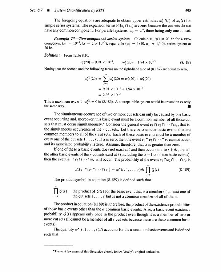
Sec. 8.7 • System Quantification by KI1T 405
The foregoing equations are adequate to obtain upper estimates w~l)(t) of ws(t) forsimple series systems: The expansion terms Pr{ej nek} are zero because the cut sets do nothave any common component. For parallel systems, Ws == w*, there being only one cut set.
Example 23-Two-component series system. Calculate w~1)(t) at 20 hr for a two-component (AI = 10-3, A2 = 2 x 10⁻³), repairable (J.lI = 1/10, J.l2 = 1/40), series system at20 hr.
Solution: FromTable8.10,
w~(20) = 9.91 x 10⁻⁴, wi(20) = 1.94 x 10⁻³ (8.188)
Noting that the second and the following terms on the right-handside of (8.187) are equal to zero,m
w~1)(20) = L wj(20) = w~(20) + wi (20)j=l
= 9.91 X 10⁻⁴ + 1.94 X 10-3
= 2.93 X 10⁻³
This is maximumws ' with W;2) = 0 in (8.186). A nonrepairable system would be treated in exactlythe same way. •
The simultaneous occurrence of two or more cut sets can only be caused by one basicevent occurring and, moreover, this basic event must be a common member of all those cutsets that must occur simultaneously.* Consider the general event el n ei n ... n er , that is,the simultaneous occurrence of the r cut sets. Let there be a unique basic events that arecommon members to all of the r cut sets: Each of these basic events must be a member ofevery one of the cut sets 1, ... , r. If a is zero, then the event el n ei n ... ne; cannot occur,and its associated probability is zero. Assume, therefore, that a is greater than zero.
If one of these a basic events does not exist at t and then occurs in t to t +d t , and allthe other basic events of the r cut sets exist at t (including the a-I common basic events),then the event el n ezn ... n e, will occur. The probability of the event el n ezn ... n e. is
*Pr{el n ei n··· n erl == w*(t; 1, ... , r)dt nQ(t)
I···r
The product symbol in equation (8.189) is defined such that
(8.189)
*nQ(t) == the product of Q(t) for the basic event that is a member of at least one ofi···r the cut sets 1, ... , r but is not a common member of all of them.
The product in equation (8.189) is, therefore, the product of the existence probabilitiesof those basic events other than the a common basic events. Also, a basic event existenceprobability Q(t) appears only once in the product even though it is a member of two ormore cut sets (it cannot be a member of all r cut sets because these are the a common basicevents).
The quantity w* (r: 1, ... , r)dt accounts for the a common basic events and is definedsuch that
"The next few pages of this discussion closely follow Vesely's original derivation.
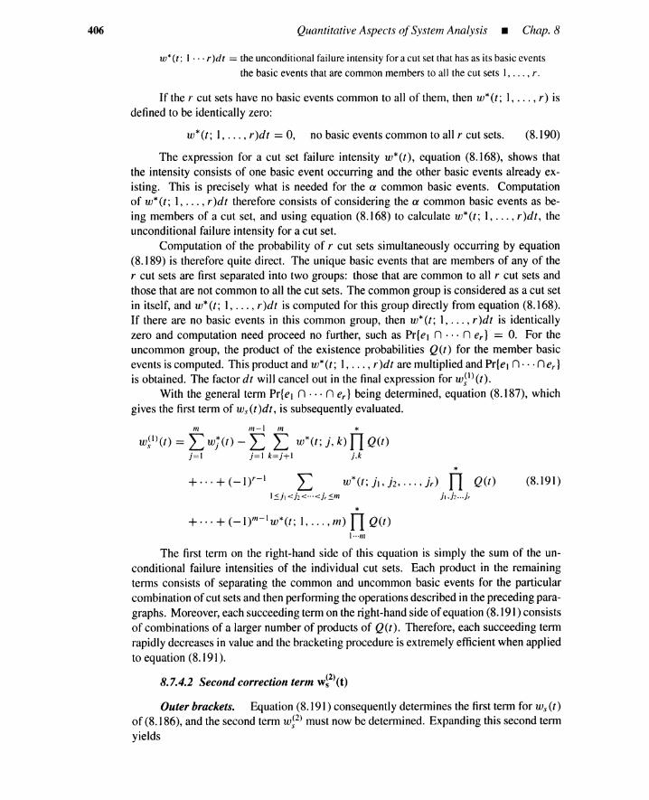
406 Quantitative Aspects ofSystem Analysis • Chap. 8
w*(t; 1... r)dt = the unconditional failure intensity for a cut set that has as its basic eventsthe basic events that are common members to all the cut sets 1, ... , r.
If the r cut sets have no basic events common to all of them, then w*(t; 1, ... , r) isdefined to be identically zero:
w*(t; 1, ... , r)dt = 0, no basic events common to all r cut sets. (8.190)
The expression for a cut set failure intensity w*(t), equation (8.168), shows thatthe intensity consists of one basic event occurring and the other basic events already ex-isting. This is precisely what is needed for the a common basic events. Computationof w* (r; 1, ... , r)d t therefore consists of considering the a common basic events as be-ing members of a cut set, and using equation (8.168) to calculate w* (t; 1, ... , r)dt, theunconditional failure intensity for a cut set.
Computation of the probability of r cut sets simultaneously occurring by equation(8.189) is therefore quite direct. The unique basic events that are members of any of ther cut sets are first separated into two groups: those that are common to all r cut sets andthose that are not common to all the cut sets. The common group is considered as a cut setin itself, and w* (r: 1, ... , r)dt is computed for this group directly from equation (8.168).If there are no basic events in this common group, then w*(t; 1, , r)dt is identicallyzero and computation need proceed no further, such as Pr{el n n er } = O. For theuncommon group, the product of the existence probabilities Q(t) for the member basicevents is computed. This product and w*(t; 1, ... , r)dt are multiplied and Pr{el n· .. ner }
is obtained. The factor dt will cancel out in the final expression for w.~l)(t).
With the general term Pr{el n ... n e.] being determined, equation (8.187), whichgives the first term of ui, (t )dt, is subsequently evaluated.
m m-I m *W.~I)(t) = L wj(t) - L L w*(t; j, k) Il o»
j=1 j=1 k=j+1 j,k
+... + (-I)r-1*
w*(t; iv.h, ... , jr) n Q(t) (8.191 )
*+···+(-I)m-I w*(t; l, ... ,m) nQ(t)
I···m
The first term on the right-hand side of this equation is simply the sum of the un-conditional failure intensities of the individual cut sets. Each product in the remainingterms consists of separating the common and uncommon basic events for the particularcombination of cut sets and then performing the operations described in the preceding para-graphs. Moreover, each succeeding term on the right-hand side of equation (8.191) consistsof combinations of a larger number of products of Q(t). Therefore, each succeeding termrapidly decreases in value and the bracketing procedure is extremely efficient when appliedto equation (8.191).
8.7.4.2 Second correction term w~2)(t)
Outer brackets. Equation (8.191) consequently determines the first term for W s (r)of (8.186), and the second term w.?) must now be determined. Expanding this second termyields

Sec. 8.7 • System Quantification by KI1T
w~2)(t)dt =pr!T0 ej !1=1
m m-l m= L Pr{ej n T} - L L Pr{ej n ekn T}
j=1 j=1 k=j+l
407
(8.192)
+ ... + (_I)r-l
l..sjl <l:< ..<irsm
+ ... + (-I)m-1pr{el n e2 n··· n em n T}
Consider a general term in this expression Pr{el n ... n e, n T}. This term is theprobability of the r cut sets simultaneously occurring in t to t + dt with one or more of theother cut sets already existing at time t (event T).
Inner brackets. Because event T involves a union, the general term may be ex-panded:
m
Pr{el n ... n e, n T} = L Pr{el n ... n e; n dj}j=1
m-l m- L L Pr{el n··· n e, n dj n dk }
j=1 k=j+l
+.··+(_I)s-1 Ll..sjl <ii« ..<i.s».
(8.193)
x Pr{el n ... n er n dh n dh n ... n djs}+ ... + (-1)m-1pr{el n ... n e, n d, n di n ... n dm}
where dj is the event of the jth cut set failure existing at time t. Consider now a generalterm in this expansion, Pr{el n ... n er n d, n ... ds }. If this term is evaluated thenPr{el n··· n er n T} will be determined and, hence, w~2)(t)dt.
The event Pr]«, n ... n er n d, n ds } is similar to the event Pr{el n ... n e.] withthe exception that now the cut sets 1, , s must also exist at time t. If a cut set existsat time t, all its basic events must exist at time t, and these basic events cannot occur int to t + dt because an occurrence calls for a nonexistence at t and then an existence att + dt. The expression for Prle, n ... n er n di n ... ds } is, therefore, analogous to theprevious expression for Pr{el n ... n e.] [eq. (8.189)] with one alteration. Those basicevents common to all the r cut sets 1, ... , r , which are also in any of the s cut sets 1, ... , s,cannot contribute to Pr{el n ... n e, n d, n ... ds } because they must already exist at timet (for the event d, n ... nds ) . Hence these basic events, common to all r cut sets and alsoin any of the s cut sets, must be deleted from w* (r: 1, ... , r) and must be incorporated inthe product of basic event existence probabilities appearing in equation (8.189).
8.7.4.3 Bracketing procedure. For fault trees with a large number of cut sets, thebracketing procedure is an extremely efficient method of obtaining as tight an envelopeas desired for W s (r). In equations (8.191), (8.192), and (8.193), an upper bound can beobtained for w~l)(t), w~2)(t), or Pr{el n ... n e, n T} by considering just the first terms inthe respective right-hand expressions. Lower bounds can be obtained by considering the
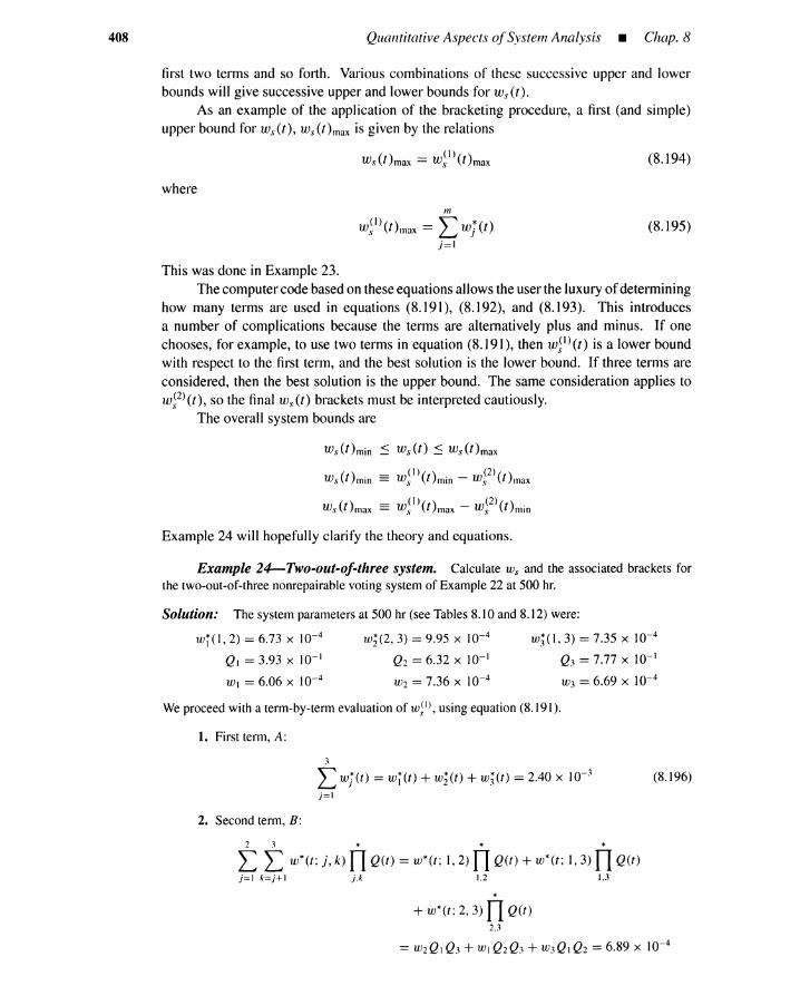
408 Quantitative Aspects ofSystem Analysis _ Chap. 8
first two terms and so forth, Various combinations of these successive upper and lowerbounds will give successive upper and lower bounds for ws(t).
As an example of the application of the bracketing procedure, a first (and simple)upper bound for ws(t), ws(t)max is given by the relations
where
W s (t )max == w.~ 1) (t )max
In
w.~I)(t)max == L wj(t)j=l
(8.194)
(8.195)
This was done in Example 23.The computer code based on these equations allows the user the luxury of determining
how many terms are used in equations (8.191), (8.192), and (8.193). This introducesa number of complications because the terms are alternatively plus and minus. If onechooses, for example, to use two terms in equation (8.191), then w.~1) (r) is a lower boundwith respect to the first term, and the best solution is the lower bound. If three terms areconsidered, then the best solution is the upper bound. The same consideration applies tow.~2) (t), so the final ui, (t) brackets must be interpreted cautiously.
The overall system bounds are
( ) _ ( I) ( ) (2) ( )Ws t min = W.\' t min - W.\' t max
( ) _ (I) ( ) (2) ( )in, t max = Ws t max - W.\' t min
Example 24 will hopefully clarify the theory and equations.
Example 24-Two-out-of-three system. Calculate ui, and the associated brackets forthe two-out-of-three nonrepairable voting system of Example 22 at 500 hr.
Solution: The system parameters at 500 hr (see Tables 8.10 and 8.12) were:
wr(l, 2) = 6.73 X 10⁻⁴ w~(2, 3) = 9.95 X 10⁻⁴ w;(I, 3) = 7.35 X 10⁻⁴
Q1 = 3.93 X 10- 1 Q2 = 6.32 X 10- 1 Q3 = 7.77 X 10- 1
W1 = 6.06 X 10⁻⁴ UJ2 = 7.36 X 10⁻⁴ w3 = 6.69 X 10⁻⁴
We proceed with a term-by-termevaluation of W.~I), using equation (8.191).
1. First term, A:
3
L wj(t) = w~(t) + w~(t) + w;(t) = 2.40 x 10⁻³
j=1
2. Second term, B:
2 3 * * *L L w*(t: i. k) nQU) = w*(t; 1,2)nQ(t) + w*U; 1,3)nQ(t)i>1 k= j+ 1 j.k 1.2 1.3
(8.196)
*+ w*(t; 2,3)nQ(t)
2.3
= W2Q1 Q3 + WI Q2Q3 + W3Q1 Q2 = 6.89 X 10⁻⁴

Sec. 8.7 • System Quantification by KIIT
3. Third term, C:
1 2 3 *L L L w*(t; j, k, l) nQ(t) = w*(t; 1,2,3)nQ(t) = O· Ql Q2Q3 = 0j=1 k=j+l1=k+l j.k.! 1.2.3
The calculation of W;2) (t) is done by using equations (8.192) and (8.193).
4. First term, D:
tPr{ej n T} = t [tpr{ej ndk} - t ItI Pr{ej ndk ndl }
1 2 3 ]
+ t;I~l q~1 Pr{ej n dk n dl n dq }
409
Recall now that ej is the event of the jth cut set failure occurring in t to t + dt , and dj is theevent of the jth cut set failure existing at t, The first term in the inner bracket is
j = 1; Pr{el n d1} + Pr{el n d2}+ Pr{el n d3} = 0 + WIQ2Q3 + W2Ql Q3
If, for example, d, exists at time t, components 1 and 2 have failed, and Pr{el} = 0 (term 1). If diexists, components 2 and 3 have failed, and only component 1 can fail, and so on. The second termin the inner bracket is zero because if two cut sets have failed, all components have failed. This istrue of term 3 also.
j = 2; Pr{e2 n d1} + Pr{e2 n d2}+ Pr{e2 n d3} = W3Ql Q2 + 0 + W2Ql Q3
j = 3; Pr{e3 ndd + Pr{e3 nd2} + Pr{e3 nd3} = W3Ql Q2 + WIQ2Q3 +03
L Pr{ej n T} = 2[W3Ql Q2 + WIQ2Q3 + W2Ql Q3] = 1.38 x 10- 3
j=1
5. Second term, E:
(a) L:=I L~=j+l Pr{ejnekn T} = L:=l L~=j+l [L;=l Pr{ej n e, n dl } - L~=l L~=I+l
x Pr{ej n ek n di n dq } + L:=l L~=I+l L~=q+1 Pr(ej n ek n dl n dq n d,} ]
(b) j = 1, k = 2; Pr{el n e2 n dd + Pr{el n e2 n d2}+ Pr{el n ei n d3}- Pr{elne2 nd1nd2}- Pr{elne2 nd1 nd3} - Pr{elne2 nd2nd3}+higher order terms(all zero) = 0 + 0 + W2Ql Q3 - 0 - 0 - 0 + 0
(c) j = 1, k = 3; Pr{el n e3 n dd + Pr{el n e3 n d2}+ Pr{el n e3 n d3}- Pr{el ne3 Csd, nd2}- Pr{el ne3 nd1nd3} - Pr{elne3 nd2nd3 } +higher order terms(all zero) = 0 + WIQ2Q3 + 0 - 0 - 0 - 0 + 0
(d) j = 2, k = 3; Pr{e2 n e3 n d1} + Pr{e2 n e3n d2}+ Pr{e2 n e3 n d3}- Pr{e2ne3ndl nd2} -Pr{e2ne3 nd1 nd3}- Pr{e2ne3nd2 nd3 }+higher order terms(all zero) = W3Ql Q2 + 0 + 0 - 0 - 0 - 0 + 0
(e) L~=1 L~=j+l Pr{ej n ek n T} = W2 Ql Q3 + WIQ2Q3 + W3 Ql Q2 = 0.5 x [D](0 iu, = W;1)-W~2) == [A-B+C]-[D-E] = 1.71 x 10⁻³-6.9x 10-4 = 1.02 x 10⁻³
•It appears that there is an error in the original KITT code subroutine that pro-
duces W}2).
8.7.5 Other System Parameters
Once Qs and ui, have been computed, it is comparatively easy to obtain the othersystem parameters, As and Ws. As with A*(t)dt, its cut set analog, the probability that the

410 Quantitative Aspects of System Analysis • Chap. 8
top event occurs in time t to t + dt, given there is no top event failure at t, is related tows(t)dt and Q.,.(t) by
ws(t)A,,(t) = I - Qs(t) (8.197)
(8.198)
•
This is identical to equation (8.169), the cut set analog. For the failure to occur in t tot +dt, (ws(t)dt), it must not exist at time t, (I - Qs(t», and must occur in time t to t +dt,
(As(t)dt).
The integral value \tV,. (0, t) is, as before, obtained from the differential ui, (t) by
w.,.(O, t) =11
w.,(u)du
Example 25-Two-out-of-three system. Calculate As(t) at 500 hr for the two-out-of-three nonrepairable votingsystem of Example22, using Qs and ui, valuesfrom Examples22 and 24.
Solution: Using the KIlT in, value from Example 24 and Q.\, from Example 22:
O_ u), _ 1.02 X 10⁻³ 1
As(50 ) - 1 _ Q.\. - 1 _ 6.59 X 10- 1 = 2.99 x 10-'
8.7.6 Short-Cut Calculation Methods
Back-of-the-envelopeguesstimates have a time-honored role in engineering and willalways be with us, computers notwithstanding. In this section we develop a modifiedversion of a calculation technique originated by Fussell [8]. It requires as input failure andrepair rates for each component and minimal cut sets. It assumes exponential distributionswith rates A and J1- and independence of component failures. We begin the derivation byrestating a few equations presented earlier in this chapter and Table 6.10. We use Qi as thesymbol for component unavailability. Suffix i refers to a component; suffix j to a cut set.As shown in Figure 8.26, for nonrepairable component i,
Qi == I - e-A;f ~ Ait
If the component is repairable,
A'Qi == __'_ [1 - e-(A;+JL;)f]
Ai + J1-i
As t becomes large and if Ai/ J1-i < < I,
Ai AiQ. ~ --- ~-1 - Ai + J1-i - J1-i
(8.199)
(8.200)
(8.201)
Figure 8.27 shows an approximation for A == 0.003 and J1- == 1/60. These approximationsfor nonrepairable and repairable cases overpredict Qi, in general.
To obtain the cut set reliability parameters, we write the familiar
/l
Q~ == no,.Ii=l
(8.202)
Equation (8.202), coupled withequation (8.201), givesthe steady-state valuefor Qjdirectly.To calculate the other cut set parameters, further approximations need to be made.
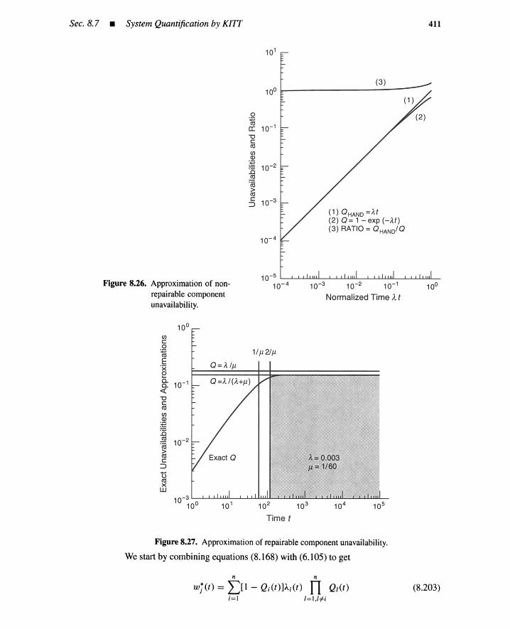
Sec. 8.7 • System Quantification by K/7T 411
(3)10°1::--------------
(1) QHAND =At(2) Q = 1 - exp (- M)(3) RATIO =Q HAND/Q
10- 5
Figure 8.26. Approximation of non- 10- 4 10-3 10- 2 10-1 10°repairable component Normalized Time Atunavailability.
10°(/lc:0
1/Jl 2/Jl~E Q d IJl'xec. 10- 1c.«"0c:ctl(/l
~:c.!!l 10- 2'ro>ctl A= 0.003c:
::::> Jl = 1/60Uctlx
W
10- 3
102 10510°
Time t
Figure 8.27. Approximation of repairable component unavailability.
We start by combining equations (8.168) with (6.105) to get
n n
wj(t) = l)1 - Q ;(t)]A;(t) n Q/{t );= 1 /=1,/# ;
(8.203)
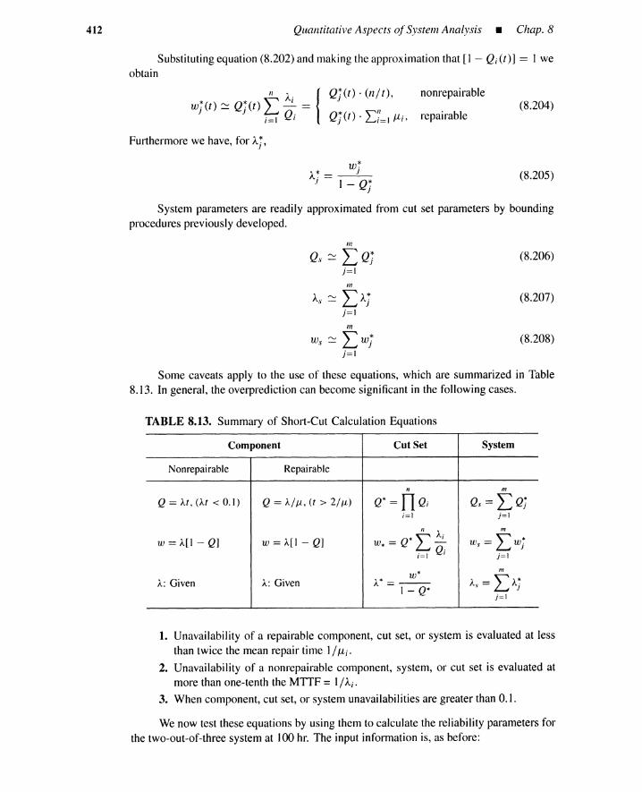
412 Quantitative Aspects ofSystem Analysis • Chap. 8
Substituting equation (8.202) and making the approximation that [I - Q;(t)] =: I weobtain
11 A Iwj(t) ::::: Qj(t) L ~ =;=1 Q,
Furthermore we have, for Aj,
Qj(t) . tnf t),
Qj(t) . l:;1=1 IJ-;,
nonrepairable
repairable(8.204)
w~)...~ =: __J_
.I I - Q~J
(8.205)
System parameters are readily approximated from cut set parameters by boundingprocedures previously developed.
m
Q.\, ~ LQj.i=1
III
A.\, ~ LAj.i=1
m
ui; ~ Lwj.i=1
(8.206)
(8.207)
(8.208)
Some caveats apply to the use of these equations, which are summarized in Table8.13. In general, the overprediction can become significant in the following cases.
TABLE 8.13. Summary of Short-Cut Calculation Equations
Component Cut Set System
Nonrepairable Repairable
n m
Q = At, (At < 0.1) Q = AI IJ.., (t > 2/JL) Q* = nQ; a. = L Qj;=1 j=1
* n A;m
W = A[l - Q] W = A[l - Q] W*= Q L- iu, = L wj;=1 Q; j=1
W*m
A: Given A: Given A*=-- As = LAj1 - Q*
j=1
1. Unavailability of a repairable component, cut set, or system is evaluated at lessthan twice the mean repair time 1/ IJ-i.
2. Unavailability of a nonrepairable component, system, or cut set is evaluated atmore than one-tenth the MTTF = 1/)...;.
3. When component, cut set, or system unavailabilitiesare greater than 0.1.
We now test these equations by using them to calculate the reliability parameters forthe two-out-of-three system at 100 hr. The input information is, as before:

Sec. 8.7 • System Quantification by KITI
Component
123
10-3
2 X 10⁻³
3 X 10⁻³
1/101/401/60
413
Cut sets are {I, 2}, {2, 3}, {I, 3}.The calculations are summarized in Table 8.14. The test example is a particularly
severe one because, at 100 hr, we are below the minimum time required by component 3 tocome to steady state (t = 100 = 1.67 x 60 = 1.67 x (1/J-l3)). As shown in Table 8.14, wesee that Qs has been calculated conservatively to an accuracy of 30%.
TABLE 8.14. Repairable and Nonrepairable Cases for Short-Cut Calculations
Numerical Exact Time Bounds to EnsureResult Value Small Overprediction
Parameter Approximation (Short-Cut) (Computer) Minimum I Maximum
Nonrepairable Case
Ql Al t 10-1 0.95 X 10⁻¹ 0 100Q2 A2 t 2 x 10⁻¹ 1.8 X 10⁻¹ 0 50Q3 A3 t 3 x 10⁻¹ 2.6 X 10⁻¹ 0 33Qr QIQ2 2 x 10⁻² 1.8 X 10⁻²
Q~ Q2Q3 6 X 10⁻² 4.7 X 10⁻²
Q; QIQ3 3 X 10⁻² 2.5 X 10⁻²
w* Q~ L(A;IQ;) 4 x 10⁻⁴ 3.2 X 10-41
w* Q~ L(A;IQ;) 12 x 10-4 8.3 X 10-42
w* Qi L(A;IQ;) 6 x 10⁻⁴ 4.5 X 10-43
Qs LQj 11 x 10-2 9 X 10⁻²
Ws LWj 2.2 X 10⁻³ 1.5 X 10⁻³
Repairable Case
Ql Al 1/1-1 10 x 10-3 9.9 X 10⁻³ 20 00
Qz AzI/1-z 80 x 10-3 74 X 10-3 80 00
Q3 A31/1-3 180 x 10-3 152 X 10-3 120 00
Qr QIQ2 8 x 10⁻⁴ 7.3 X 10⁻⁴
Q~ Q2Q3 14.4 X 10⁻³ 11 X 10-3
Q; QIQ3 1.8 X 10⁻³ 1.5 X 10⁻³
w* Qr L (A; I Q;) 10 X 10-5 9.2 X 10-51
w* Q~ L(A;IQ;) 6 x 10⁻⁴ 4.2 X 10⁻⁴z
w* Qi L(A;IQ;) 2.1 x 10⁻⁴ 1.8 X 10-43
Qs LQj 17 x 10-3 13 X 10-3
Ws LWj 9.1 X 10⁻⁴ 7 X 10⁻⁴
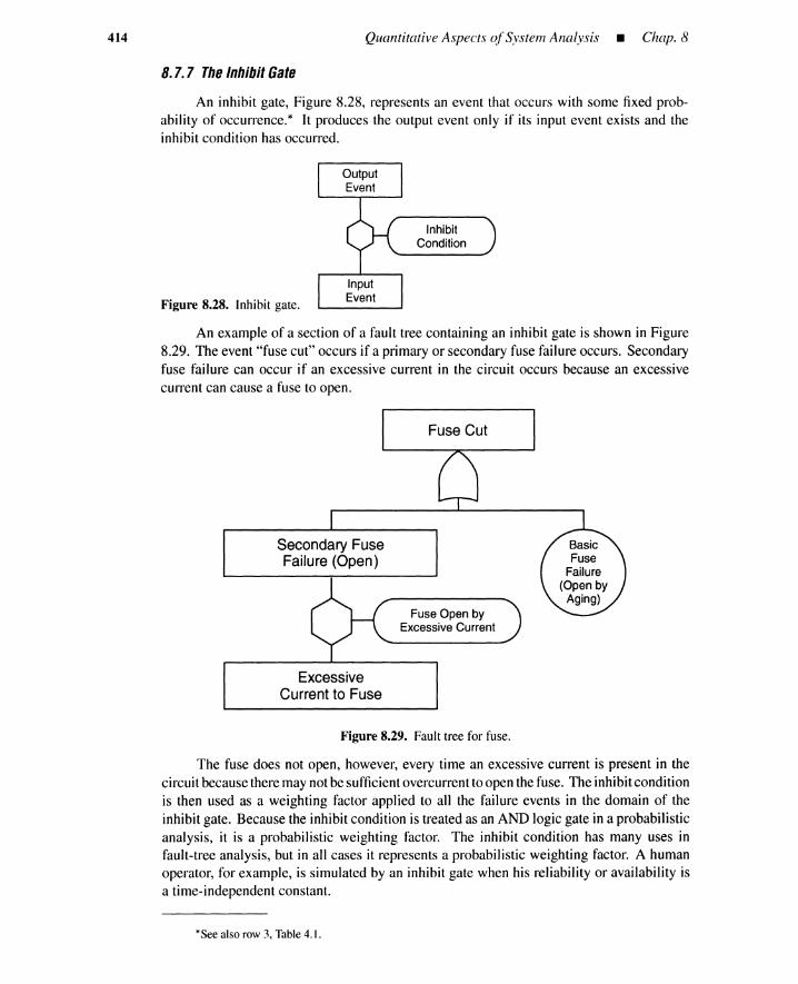
414 Quantitative Aspects ofSystem Analysis • Chap. 8
8.7.7 The InhibitGate
An inhibit gate, Figure 8.28, represents an event that occurs with some fixed prob-ability of occurrence.* It produces the output event only if its input event exists and theinhibit condition has occurred.
InhibitCondition
Figure 8.28. Inhibit gate.
An example of a section of a fault tree containing an inhibit gate is shown in Figure8.29. The event "fuse cut" occurs if a primary or secondary fuse failure occurs. Secondaryfuse failure can occur if an excessive current in the circuit occurs because an excessivecurrent can cause a fuse to open.
Fuse Cut
Fuse Open byExcessive Current
Secondary FuseFailure (Open)
ExcessiveCurrent to Fuse
Figure 8.29. Fault tree for fuse.
The fuse does not open, however, every time an excessive current is present in thecircuit because there maynot be sufficientovercurrentto open the fuse. The inhibitconditionis then used as a weighting factor applied to all the failure events in the domain of theinhibit gate. Because the inhibit condition is treated as an AND logic gate in a probabilisticanalysis, it is a probabilistic weighting factor. The inhibit condition has many uses infault-tree analysis, but in all cases it represents a probabilistic weighting factor. A humanoperator, for example, is simulated by an inhibit gate when his reliability or availability isa time-independent constant.
*See also row 3, Table 4.1.

Sec. 8.7 • System Quantification by KIIT 415
If, in the input to KITT, an event is identified as an inhibit condition, the cut setparameters Q* and w* are multiplied by the inhibit value. In the two-component parallelsystem of Figure 8.30, a value of 0.1 is assigned to the inhibit condition, Q2 = 0.1. Theresults of the computations are summarized in Table 8.15. We see that the effect of theinhibit gate in Figure 8.30 is to yield Q* = QI Q2 = QI x 0.1 and w* = WI x 0.1, withQ2 independent of time.
Figure 8.30. Example system withinhibit gate.
TABLE 8.15. Computation for Inhibit Gate
Time Qt Wt Qs Ws
20 8.59 X 10⁻³ 9.91 X 10⁻⁴ 8.59 X 10⁻⁴ 9.91 X 10⁻⁵
500 9.90 X 10⁻³ 9.90 X 10⁻⁴ 9.90 X 10⁻⁴ 9.90 X 10⁻⁵
8.7.8 Remarks onQuantification Methods
8.7.8.1 Component unavailabilityfor age-dependentfailure rate. Assume a com-ponent has an age-dependent failure rate r(s), where s denotes age. The equation
w(t)r(t) - I _ Q(t) (8.209)
incorrectly quantifies unavailability Q(t) at time t, for a given r(t) and w(t). This equationis correct if r(t) is replaced by A(t), the conditional failure intensity of the component:
)..(t) = w(t)1 - Q(t)
(8.210)
(8.211 )
(8.212)
It is difficult to use this equation for the quantification of Q(t), however, because A(t) itselfis an unknown parameter. One feasible approach is to use (6.96) to quantify Q(t).
8.7.8.2 Cut set or system reliability
R(t) = exp [-l\(U)dU]This equation is not generally true. The correct equation is (6.67),
R(t) = exp [ -1/ r(U)dU]Equation (8.211) is correct only in the case where failure rate r (t) is constant and hencecoincides with the (constant) conditional failure intensity A(t) = A. For cut sets or systems,
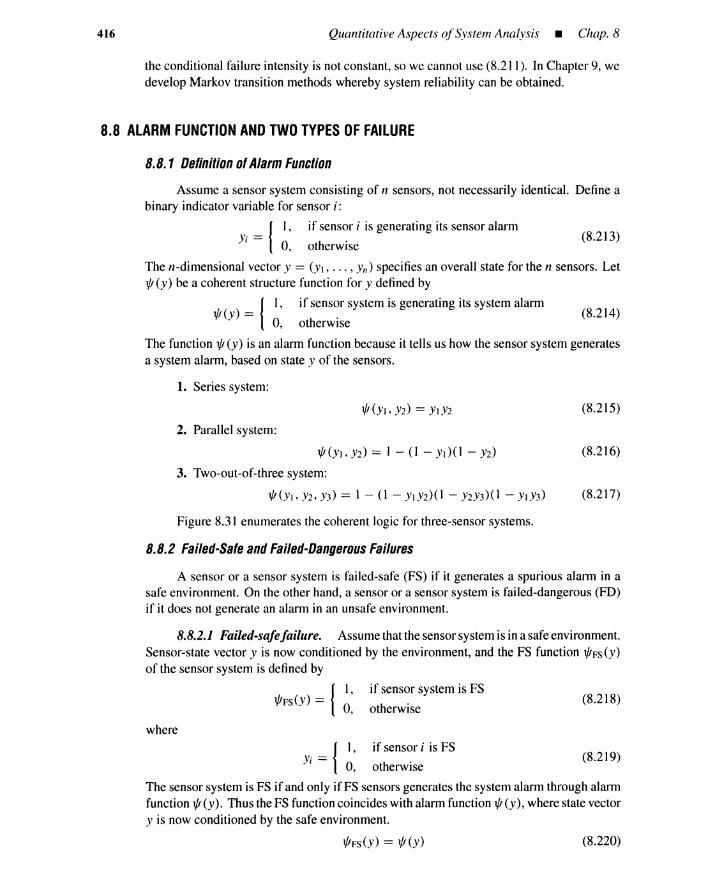
416 Quantitative Aspects ofSystem Analysis - Chap. 8
the conditional failure intensity is not constant, so we cannot use (8.211). In Chapter 9, wedevelop Markov transition methods whereby system reliability can be obtained.
(8.213)
(8.214)
8.8 ALARM FUNCTION AND TWO TYPES OF FAILURE
8.8.1 Definition ofAlarm Function
Assume a sensor system consisting of n sensors, not necessarily identical. Define abinary indicator variable for sensor i:
{I , if sensor i is generating its sensor alarm
Yi == 0, otherwise
The n-dimensional vector Y == (YI, ... , Yn) specifies an overall state for the n sensors. Let1/1 (y) be a coherent structure function for Y defined by
{I , if sensor system is generating its system alarm
1/I(y) == .0, otherwise
The function 1/1 (y) is an alarm function because it tells us how the sensor system generatesa system alarm, based on state Y of the sensors.
1. Series system:
2. Parallel system:
1/1 (y I , Y2) == 1 - (1 - y I ) (I - Y2)
3. Two-out-of-three system:
1/I(YI,Y2, Y3) == 1 - (I - YIY2)(1 - Y2Y3)(1 - YIY3)
Figure 8.31 enumerates the coherent logic for three-sensor systems.
8.8.2 Failed-Safe and Failed-Dangerous Failures
(8.215)
(8.216)
(8.217)
(8.218)
A sensor or a sensor system is failed-safe (FS) if it generates a spurious alarm in asafe environment. On the other hand, a sensor or a sensor system is failed-dangerous (FD)if it does not generate an alarm in an unsafe environment.
8.8.2.1 Failed-safefailure. Assume that the sensor system is in a safe environment.Sensor-state vector Y is now conditioned by the environment, and the FS function 1/IFS (y)of the sensor system is defined by
{I , if sensor system is FS
1/IFS (Y) == 0, otherwise
where
{I , if sensor i is FS
Y· - (8.219)I - 0, otherwise
The sensor system is FS if and only if FS sensors generates the system alarm through alarmfunction 1/1 (y). Thus the FS function coincides with alarm function 1/1 (y), where state vectory is now conditioned by the safe environment.
1/IFS (y) == 1/1 (y) (8.220)
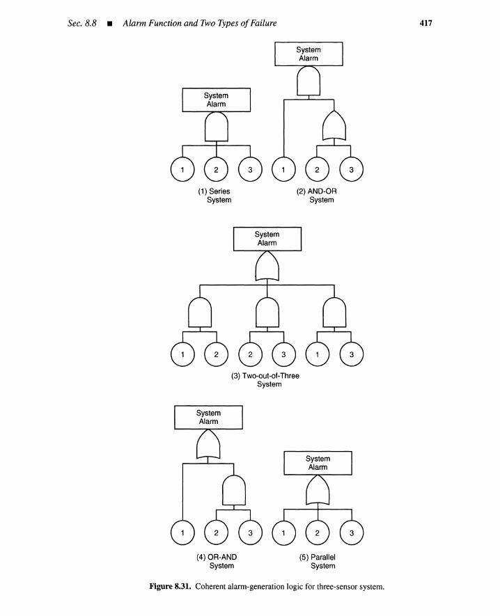
Sec. 8.8 • Alarm Function and Two Types ofFailure 417
(1) SeriesSystem
(2) AND-ORSystem
(3) Two-out-of-ThreeSystem
(4) OR-ANDSystem
(5) ParallelSystem
Figure 8.31. Coherent alarm-generation logic for three-sensorsystem.
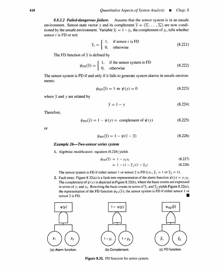
418 Quantitative Aspects ofSystem Analysis - Chap. 8
8.8.2.2 Failed-dangerous failure. Assume that the sensor system is in an unsafeenvironment. Sensor-state vector y and its complement Y == (Yl, ... ,Yn) are now condi-tioned by the unsafe environment. Variable Yi == 1- Yi, the complement of Yi, tells whethersensor i is FD or not:
_ {I,Yi == 0,
The FD function of y is defined by
if sensor i is FD
otherwise(8.221)
{I ,
l/JFo (Y) == 0,if the sensor system is FD
otherwise(8.222)
The sensor system is FD if and only if it fails to generate system alarms in unsafe environ-ments:
l/JFO (Y) == 1 <=> l/J (y) == °where y and yare related by
y==l-y
Therefore,
l/JFD(Y) == I - l/J (y) == complement of l/J (y)
or
l/JFD(Y) == 1 - l/J( 1 - Y)
Example 26-Two-sensor series system
1. Algebraic modification: equation (8.226) yields
1/IrD(Y) = 1 - YlY2
1 - (I - Yl)(1 - Y2)
(8.223)
(8.224)
(8.225)
(8.226)
(8.227)
(8.228)
The sensor system is FD if either sensor 1 or sensor 2 is FD (i.e., Yl = 1 or Y2 = 1).
2. Fault trees: Figure 8.32(a) is a fault-tree representation of the alarm function 1/I(y) = YlY2.The complement of 1/1 (Y) is depicted in Figure 8.32(b), where the basic events are expressedin terms of Yl and Y2. Rewriting the basic events in terms OfYl and Y2yields Figure 8.32(c),the representation of the FD function 1/I..n(Y); the sensor system is FD if either sensor I orsensor 2 is FD. •
(a) Alarm function. (b) Complement.
Figure 8.32. FD function for series system.
(c) FD function.
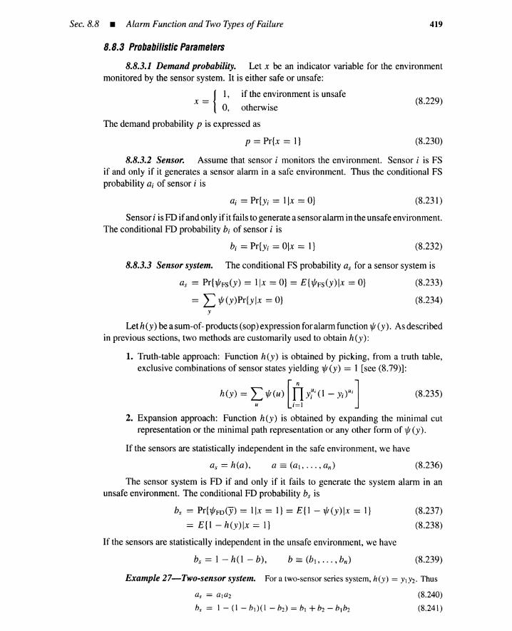
Sec. 8.8 • Alarm Functionand Two Types ofFailure
8.8.3 Probabilistic Parameters
419
8.8.3.1 Demand probability. Let x be an indicator variable for the environmentmonitored by the sensor system. It is either safe or unsafe:
X__ { I, if the environment is unsafe
(8.229)0, otherwise
The demand probability p is expressed as
p == Pr{x == I} (8.230)
8.8.3.2 Sensor. Assume that sensor i monitors the environment. Sensor i is FSif and only if it generates a sensor alarm in a safe environment. Thus the conditional FSprobability c, of sensor i is
ai == Pr{Yi == l lx == O} (8.231)
Sensor i is FD if and only if it fails to generate a sensor alarm in the unsafe environment.The conditional FD probability b, of sensor i is
b, == Pr{Yi == Olx == I} (8.232)
(8.233)
(8.234)
(8.235)
8.8.3.3 Sensor system. The conditional FS probability as for a sensor system is
as == Pr{l/!FS(Y) == llx == O} == E{l/!Fs(Y)lx == O}
== L VJ(y)Pr{Ylx == O}y
Let h(y) be a sum-of- products (sop) expression for alarm function l/! (y). As describedin previous sections, two methods are customarily used to obtain h(y):
1. Truth-table approach: Function h(y) is obtained by picking, from a truth table,exclusive combinations of sensor states yielding l/!(y) == 1 [see (8.79)]:
h(y) = ~1/J(U) [Oli O - "'.
2. Expansion approach: Function h(y) is obtained by expanding the minimal cutrepresentation or the minimal path representation or any other form of VJ (y).
If the sensors are statistically independent in the safe environment, we have
as == h(a), (8.236)
The sensor system is FD if and only if it fails to generate the system alarm in anunsafe environment. The conditional FD probability bs is
bs == Pr{VJFD (Y) == 11x == I} == E{I - 1/1 (y ) Ix == I}
== E{l - h(y)lx == I}
If the sensors are statistically independent in the unsafe environment, we have
(8.237)
(8.238)
bs == 1 - h(l - b), (8.239)
Example 27-Two-sensor system. For a two-sensor series system, h(y) = YIY2. Thus
(8.240)
(8.241)

420 Quantitative Aspects ofSystem Analysis _ Chap. 8
For a two-sensorparallel system, h (y) == YI + .\"2 - .vI Y2. Thus
b, == 1 - (1 - hI> - (I - h2) + (1 - hI> (1 - h2)
== h)h2
(8.242)
(8.243)
It can be shown that a series system consisting of identical sensors has fewer FS failures thana parallel system; the parallel system is less susceptible to FD failures than the series system. •
Probabilistic parameters for three-sensor systems are summarized in Table 8.16. Letus now compare alarm-generating logic, assuming identical sensors ta, == a, b, == b). Itcan be shown easily that
a(l) < a(2) < a(3) < a(4) < a(5)S - S - S - S - ·S
(8.244)
(8.245)
where superscripts have the following meanings: (1) == series system (i.e., three-out-of-three system), (2) == AND-OR system, (3) == two-out-of-three system, (4) == OR-ANDsystem, (5) == parallel system (i.e., one-out-of-three system).
TABLE 8.16. Probabilistic Parameters for Three-Sensor Systems
General Components
Parameter (1) Series (2) AND-OR (3) Two-out-of-Three (4) OR-AND (5) Parallel
Os Ol a203 al o2 + al a3 a)a2 + a.a, + a2a3 al + aias a) + a: + a3-0102a3 - 201 0203 -01a2a3 -al a2 - al a3
-a2a3 + a, aias
hs hI + b: + h3 b, + h2h3 h)h2+ h Ih3+ h2h3 h)h2+ bib, hIh2h3
-h)h2 - bib, -h lh2h3 -2h Ih2h3 -h1h2h3
-h2h3 + b,h2h3
Identical Components
as a3 2a2 - a3 302 - 203 a + a2 - a3 3a - 3a2+ a3
h,\' 3h - 3h2+ h3 h + h2 - h3 3h2 - 2h3 2h2 - h3 h3
REFERENCES
[I] Vesely, W. E. "A time-dependent methodology for fault tree evaluation," NuclearEngineering and Design, vol. 13, no. 2, pp. 337-360, 1970.
[2] Caceres, S., and E. J. Henley. "Process analysis by block diagrams and fault trees,"Industrial Engineering Chemistry: Fundamentals, vol. 15, no. 2, pp. 128-133,1976.
[3] Esary, J. D., and F. Proschan. "Coherent structures with non-identical components,"Technometrics, vol. 5, pp. 191-209, 1963.
[4] Esary, J. D., and F. Proschan. "A reliability bound for systems of maintained andindependent components," J. of the American Statistical Assoc., vol. 65, pp. 329-338,1970.
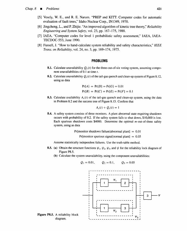
Chap. 8 • Problems 421
[5] Vesely, W. E., and R. E. Narum. "PREP and KITT: Computer codes for automaticevaluation of fault trees," Idaho Nuclear Corp., IN1349, 1970.
[6] Jingcheng, L., and P. Zhijie. "An improved algorithm of kinetic tree theory," ReliabilityEngineering and System Safety, vol. 23, pp. 167-175, 1988.
[7] IAEA. "Computer codes for level 1 probabilistic safety assessment," IAEA, IAEA-TECDOC-553, June 1990.
[8] Fussell, J. "How to hand-calculate system reliability and safety characteristics," IEEETrans. on Reliability, vol. 24, no. 3, pp. 169-174, 1975.
PROBLEMS
8.1. Calculate unavailability Qs(t) for the three-out-of-six voting system, assuming compo-nent unavailabilities of 0.1 at time t.
8.2. Calculate unavailability Qs(r) of the tail-gas quench and clean-up system of Figure 8.12,using as data
Pr{A} = Pr{D} = PrIG} = 0.01
Pr{B} = Pr{C} = Pr{E} = Pr{F} = 0.1
8.3. Calculate availability As(t) of the tail-gas quench and clean-up system, using the datain Problem 8.2 and the success tree of Figure 8.15. Confirm that
8.4. A safety system consists of three monitors. A plant abnormal state requiring shutdownoccurs with probability of 0.2. If the safety system fails to shut down, $10,000 is lost.Each spurious shutdown costs $4000. Determine the optimal m-out-of-three safetysystem, using as data
Pr{monitor shutdown failurelabnormal plant} = 0.01
Pr{monitor spurious signallnormal plant} = 0.05
Assume statistically independent failures. Use the truth-table method.
8.5. (a) Obtain the structure functions l/JI' l/J2, l/J3' and l/J for the reliability lock diagram ofFigure P8.5.
(b) Calculate the system unavailability, using the component unavailabilities:
QI =0.01, Q2 = 0.1, Q3 = 0.05
Figure P8.5. A reliability blockdiagram.
I----------------~
1 11 1
11
1 1' J
I----------------~
1 11 I
11
1 I1 J
1JI3

422 Quantitative Aspects ofSystem Analysis - Chap. 8
8.6. Consider the reliability block diagram of Figure P8.6. Assume stationary unavailabili-ties:
Figure P8.6. A bridge circuit.
(a) Obtain minimal cuts and minimal paths by inspection.(b) Determine the minimalcut and minimalpath representationof the structure function.(c) Calculate the system unavailability by expanding the two structure functions.(d) Obtain the system unavailabilityby the partial pivotaldecomposition of the minimal
cut representation.(e) Calculate each bracket of the inclusion-exclusion principle. Obtain the successive
lower and upper bounds. Obtain the Esary and Proschan lower and upper bound aswell.
(0 Obtain lower and upper bounds using two-event minimal cut sets and minimal pathsets.
(g) Assumeconstant failurerates (conditional failure intensities), Al == A2 == A3 == A4 ==A5 == 0.0 I. Obtain constant repair rates (conditional repair intensities), J-tl' ... , J-t5.
8.7. Assume the following rates for the bridge circuit of Figure P8.6.
AI == A2 == A3 == A4 == A5 == 0.00 I == A
J-tl == 112 == 113 == 114 == J-t5 == 0.0 I == u.
(a) Obtain component parameters Qi, ui., and Vi at t == 100.(b) The bridge circuit has four minimal cut sets: K1 == {I, 2}, K2 == {3,4}, K3 ==
{I, 4, 5}, and K4 == {2, 3, 5}. Calculate cut set parameters Q;, w;, A;, v;, and J-t; att == 100.
(c) Define by
el : cut set {I, 2} occurs at time t
e: : cut set {3,4} occurs at time t
e3 : cut set {I, 4, 5} occurs at time t
e4 : cut set {2, 3, 5} occurs at time t
Show that w.~l) (t )dt of (8.187) becomes
UJ.~I)(t)dt == PrIed + Pr{e2} + Pr{e3} + Pr{e4}
- Pr[e, n e2} - Pr{el n e3} - Pr{el n e4}
- Pr{e2 n e3} - Pr{e2 n e4} - Pr{e3 n e4}
+ Pr{e) n e: n e3} + Pr{el n e2 n e4} + Pr{el n e3 n e4}
+ Pr{e2 n e3 n e4} - Pr{el n ei n e3 n e4}
(d) Determine common members for each term on the right-hand side of the aboveexpression. Determine also w*(t: I, ... , r) and n~ ...r Q(t) of(8.189).
(e) Calculate lower and upper bounds for w.~\)(IOO), using as data:
Qi(IOO) == 6.06 x 10⁻², wi(IOO) == 9.39 x 10⁻⁴, i == 1, ... ,5
w;(I00) == w2(100) == 1.14 x 10⁻⁴, w.~(lOO) == w;(IOO) == 1.04 x 10⁻⁵
Chap. 8 • Problems 423
8.8. (a) If cut sets Kh , ... , Kjr have no common members, then Pr{eh n ... n ejr n T} in(8.192) is zero. Noting this, show for the bridge circuit of Figure P8.6 that
w;2)(t) = Pr{el n T} + Pr{e2n T} + Pr{e3n T} + Pr{e4 n T}
-Pr{el n e3 n T} - Pr{el n e4 n T} - Pr{e2 n e3 n T}
-Pr{e2 n e4n T} - Pr{e3n e4n T}
(b) Expand each term in the above equation, and simplify the results.(e) Obtain lower and upper bounds for w~2)(100) using Qi, ui., and wj from Problem
8.7.8.9. (a) Obtain successivelower and upper bounds of W s (100) using the successivebounds:
w;1) (1OO)max.1 = 2.49 x 10⁻⁴
w;1)(IOO)min.1 = 2.48 x 10⁻⁴
w~l)(100)max.2 = 2.48 x 10-4 = w~1)(100)min.2 = last bracket
w~2)(100)max.1 = 3.28 x 10⁻⁶
W;2) (100)min.l = 3.21 x 10⁻⁶
w;2)(I 00)max.2 = 3.21 x 10-6 = w~2) (100)min.2 = last bracket
(b) Obtain an upper bound of As(100), using Qs(100)max = 7.80 x 10⁻³•
8.10. Apply the short-cut calculation of the reliability parameters for the bridge circuit ofFigure P8.6 at t = 500, assuming the rates
Al = A2 = A3 = A4 = As = 0.001 = A
J.ll = J.l2 = J.l3 = J.l4 = J.ls = 0.01 = J.l

9ystem Quantification_.for Dependent Events
9.1 DEPENDENT FAILURES
Dependent failures are classified as functional and common-unit interdependencies of com-ponents or systems, common-cause failures, and subtle dependencies.
9.1.1 Functional and Common-Unit Dependency
Functional and common-unit dependencies are called cascade failures, propagatingfailures, or command failures. They exist when a system or a component is unavailablebecause of the lack of required input from support systems. Functional and common-unitdependencies are caused by functional coupling and common-unit coupling, described inChapter 2. Most PRAs explicitly represent functional and common-unit dependencies byevent trees, fault trees, reliability block diagrams, or Boolean expressions. These rep-resentations are explicit models because cause-effect relationships are modeled explicitlyby the logic models. There are two types of functional and common-unit dependencies:intrasystem (i.e., within a system) and intersystem (i.e., between or among systems) [1].
1. Intrasystem dependencies: These are incorporated directly into the logic model.For example, the fact that a valve cannot supply water to a steam generator un-less a pump functions properly is expressed by the feedwater-system fault tree orreliability block diagram.
2. Intersystem dependencies: For this type of dependency (e.g., the dependence ofa motor-operated pump in a feedwater system on the supply of electric power),there are two approaches. If a small-event-tree approach is followed, a relativelylarge fault tree for the feedwater system can be constructed to explicitly includethe power supply failure as a cause of motor-operated pump failure. If a large-event-tree approach is used, the intersystem dependencies can be incorporated into
425

426 System Quantification for Dependent Events _ Chap. 9
the event-tree headings so that a relatively small fault tree is constructed for thefeedwater system for each different power supply state in the event tree.
9.1.2 Common-Cause Failure
Common-cause failure is defined as the simultaneous failure or unavailability of morethan one component due to shared causes other than the functional and common-unit de-pendencies already modeled in the logic model. The OCCUITence of common-cause failuresis affected by factors such as similarity or diversity of components, physical proximity orseparation of redundant components, or susceptibilities of components to environmentalstresses. An extremely important consideration is the potential for shared human error indesign, manufacture, construction, management, and operation of redundant elements.
Models are available for implicitly representing common-cause effects by modelparameters. This type of representation is called parametric modeling.
9.1.3 Subtle Dependency
Subtle dependency includes standby redundancies, common loads, and exclusivebasic events.
1. Standby redundancy: Standby redundancy is used to improve system availabilityand reliability. When an operating component fails, a standby component is putinto operation, and the system continues to function. Failure of an operatingcomponent causes a standby component to be more susceptible to failure becauseit is now under load. This means that failure of one component affects the failurecharacteristics of other components, thus component failures are not statisticallyindependent. Typically, Markov models are used to represent dependency due tostandby redundancy.
2. Common loads: Assume that a set of components supports loads such as stressesor currents. Failure of one component increases the load carried by the othercomponents. Consequently, the remaining components are more likely to fail, sowe cannot assume statistical independence. The dependency among componentscan be expressed by Markov models.
3. Mutually exclusive events. Consider the basic events, "switch fails to close" and"switch fails to open." These two basic events are mutually exclusive, that is,occurrence of one basic event precludes the other. Thus we encounter dependentbasic events when a fault tree involves mutually exclusive basic events. Thisdependency can be accounted for when minimal cut sets are obtained.
9.1.4 System-Quantification Process
The inclusion-exclusion principle, when coupled with appropriate models, enablesus to quantify systems that include dependent basic events. A general procedure for systemquantification involving dependent failures is as follows.
1. Represent system parameters by the inclusion-exclusion principle. For each termin the representation, examine whether it involves dependent basic events or not.If a term consists of independent events, quantify it by the methods in Chapter 8.Otherwise, proceed as follows.

Sec. 9.2 • Markov Model for Standby Redundancy 427
2. Model dependent events by an appropriate model.
3. Quantify terms involving dependent events by solving the model.
4. Determine the first bracket to obtain upper bounds for the system parameter. Ifpossible, calculate the second bracket for the lower bound or compute a completeexpansion of the system parameter for the exact solution.
This chapter deals with dependencies due to standby redundancies and commoncauses.
9.2 MARKOV MODEL FOR STANDBY REDUNDANCY
9.2.1 Hot, Cold, and Warm Standby
Consider the tail-gas quench and clean-up system of Figure 8.12. The correspondingfault tree is Figure 8.13. There are two quench pumps, A and B; one is in standby and theother-the principal pump-is in operation.
Assume that pump A is principal at a given time t, whereas pump B is in standby.If pump A fails, standby pump B takes the place of A, and pumping continues. The failedpump A is repaired and then put into standby when the repair is completed. Repairedstandby pump A will replace principal pump B when it fails. The redundancy increasessystem or subsystem reliability. The system has another standby redundancy consisting ofthe two circulation pumps E and F.
Each component in standby redundancy has three phases: standby, operation, andrepair. Components fail only when they are in operation (failure to run) or in standby(failure to start). Depending on component-failure characteristics during these phases,standby redundancy is classified into the following types.
1. Hot Standby: Each component has the same failure rate regardless of whether it isin standby or operation. Hot standby redundancy involves statistically independentcomponents because the failure rate of one component is unique, and not affectedby the other components.
2. Cold Standby: Components do not fail when they are in cold standby. Failure of aprincipal component forces a standby component to start operating and to have anonzero failure rate. Thus failure characteristics of one component are affected bythe other, and cold standby redundancy results in mutually dependent basic events(component failures).
3. Warm Standby: A standby component can fail, but it has a smaller failure ratethan a principal component. Failure characteristics of one component are affectedby the other, and warm standby induces dependent basic events.
9.2.2 Inclusion-Exclusion Formula
The fault tree in Figure 8.13 has five minimal cut sets:
d, == {A}, d4 == {B, C}, ds == {E, F} (9.1)
The inclusion exclusion principle (8.122) gives the following lower and upper bounds forsystem unavailability Qs(t).
(9.4)
428 System Quantificationfor Dependent Events _ Chap. 9
Qs (t )max == first bracket
== Pr{A} + Pr{D} + PrIG} + Pr{B n C} + Pr{E n F} (9.2)
Qs(l)min == Qs(l)max - second bracket (9.3)
Qs(l)max - Pr{A n D} - Pr{A n G} - Pr{A n B n C}
- Pr{A n E n F} - Pr{D n G} - Pr{D n B n C}
- Pr{D n En F} - PrIG n B n C} - PrIG n En F}
- Pr{B n C n En F}
Events A, D, G, B nC, and En F are mutually independent by assumption, thus (9.4) canbe written as
Qs(l)min == Qs(l)max - Pr{A}Pr{D} - Pr{A}Pr{G} - Pr{A}Pr{B n C}
- Pr{A}Pr{E n F} - Pr{D}Pr{G} - Pr{D}Pr{B n C}
- Pr{D}Pr{E n F} - Pr{G}Pr{B n C}
- Pr{G}Pr{E n F} - Pr{B n C}Pr{E n F}
Note that the equalities
Pr{B n C} == Pr{B}Pr{C} IPr{E n F} == Pr{E}Pr{F}
(9.5)
(9.6)
hold only for hot standby redundancy. Cold or warm standby does not satisfy these equal-ities.
Probabilities Pr{A}, Pr{D}, and Pr{G} are component unavailabilities computable bymethods in Chapter 6. Probabilities Pr{B n C} and Pr{E n F} are denoted by Q,.(l), whichis the unavailability in standby redundancy calculated by the methods explained in thefollowing sections. In all cases we assume perfect switching, although switching failurescould also be expressed by Markov transition models.
9.2.3 Tilne-OependenlUnavaffabffffy
9.2.3.1 Two-component redundancy. Figure 9.1 summarizes the behavior of astandby-redundancy system consisting of components A and B. Each rectangle representsa redundancy state. The extreme left box in a rectangle is a standby component, the middlebox is a principal component, and the extreme right box is for components under repair.Thus rectangle 1 represents a state where component B is in standby and component A isoperating. Similarly, rectangle 4 expresses the event that component B is operating andcomponent A is under repair. Possible state transitions are shown in the same figure. Thewarm or hot standby has transitions from state I to 3, or state 2 to 4, whereas the coldstandby does not. For the warm or hot standby, the standby component fails with constantfailure rate I. For hot standby, I is equal to A, the failure rate for principal components.For cold standby, X" is zero. The warm standby (0 :s X" :s A) has as its special cases the hotstandby (X" == A)and the cold standby (X" = 0). Two or less components can be repaired at atime, and each component has a constant repair rate u, In all cases, the system fails whenit enters state 5.
Denote by P;(I) the probability that the redundant system is in state i at time I. Thederivative Pi (I) is given by

Sec.9.2 • Markov Modelfor Standby Redundancy
," - - - - - - - - . Cold Standby" ,- - - - - - - In Operation
" " , - - - - - Under Repair, , ,, , ,
429
," - - - - - - - _. Warm or Hot Standby
" ,- - - - - - - In Operation
" " , - - - - - Under Repair, I I
, I I
3 3
Figure 9.1. Transitiondiagram for cold, warm, or hot standby. (a) Diagramforcold standby; (b) Diagramfor warm or hot standby.
p;(!) = (inflow to state i) - (outflow from state i)
= L [rate of transition to state i from state j] x [probability of state j]j#;
-L [rate of transition from state i to state j] x [probability of state i]j#;
(9.7)
Notice that each transition rate is weighted by the corresponding source state probability.The above formula results in a set of differential equations
PI -(A + A) 0 u. 0 0 PI
P2 0 -(A- + I) 0 u. 0 P2
P3 I A- -(A- + Ji-) 0 Ji- P3 (9.8)
P4 A- A- 0 -(A- + J.,t) J.,t P4
P5 0 0 A- A- -2J.,t P5
The first equation in (9.8) is obtained by noting that state 1 has inflow rate J.,t from state 3and two outflow rates, A- and I. Other equations are obtained in a similar way. Assume thatthe redundant system is in state 1 at time zero. Then the initial condition for (9.8) is
[PI (0), P2(O), ... , P5(0)] = (1,0, ... , 0) (9.9)
Add the first equation of (9.8) to the second, and the third equation to the fourth,respectively. Then
J.,t
-(A- + J.,t)
A-
(9.10)

430 System Quantification for Dependent Events _ Chap. 9
Define
(P(o)
)=(PI + P2
)P(I) P.., + P4
P(2) Ps
Then (9.10) can be written as
( F(O») (-(A + I) JJ- 0
)(p(o)
)~(l) == A+I -(A + JJ-) 2JJ- P(l)
P(2) 0 A -2JJ- P(2)
with the initial condition
[p(O)(O), P(l)(O), P(2)(0)] == (1,0,0)
(9.11)
(9.12)
(9.13)
The differential equations of (9.12) are for Figure 9.2, the transition diagram consisting ofstates (0), (1), and (2). State (0), for example, has outflowrate A+I and inflowrate JJ-.
(0)
(1 )
Figure 9.2. Simplified Markov transitiondiagram: redundant con- (2)figuration.
One Standby.Component andOne OperatingComponent
J1 ,1+ X
"One OperatingComponentandOne ComponentUnder Repair
~
2J1 A
"
Two Components Under Repair
Equation (9.12) can be integrated numerically or, if an analytical solution for PO) isrequired, Laplace transforms may be used. The Markovdifferentialequations representde-pendent failuresby introducingstate-dependenttransitionrates; interconnectedcomponentsdo not necessarily operate independently, nor are repairs of failed components necessar-ily made independently. For more information on Markov models, analytical solutions,numerical calculations, and reliability applications, the reader can consult the articles andtextbooks cited in reference [2].
The parameter Q,.(t) == Pr{A n B} is the unavailability of the standby redundancy{A, B} and equals the probability that both components A and B are under repair at time t.Thus
(9.14)
Example 1-Warm standby. Consider the redundant quench pumps Band C of Fig-ure 8.12. Assume the following failure and repair rates for each pump.
(9.15)
Calculate parameter Qr(t) at t = 100,500, and 1000 hr.
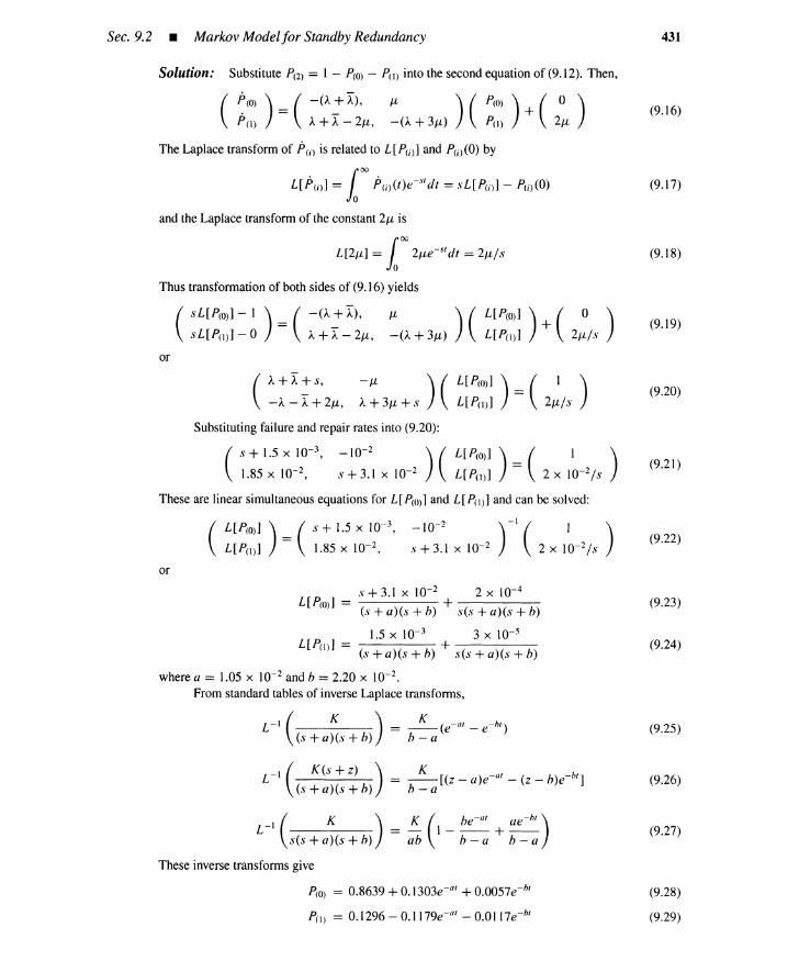
Sec. 9.2 • Markov Model for Standby Redundancy
Solution: Substitute P(2) = 1 - p(o) - P(1) into the second equation of (9.12). Then,
431
(
~(o) ) = ( -(A~I),PO) A+ A - 2/1,
(9.16)
The Laplace transform of ?(i) is related to L[P(i)] and P(i)(O) by
L[J'ti)] =100
P(j)(t)e-S'dt =sL[P(j)]- P(j)(O)
and the Laplace transform of the constant 2/1 is
L[2JL] =100
2JLe-S'dt = 2JL/s
Thus transformation of both sides of (9.16) yields
(9.17)
(9.18)
(9.19)
or
-/1
A+ 3/1+ S )( (9.20)
Substituting failure and repair rates into (9.20):
(
S + 1.5 X 10⁻³
, -10-2
) ( L[P(O)]) ( 1 ) (9.21)1.85 x 10- 2 , S + 3.1 X 10- 2 L[Po)] - 2 X 10⁻²/s
These are linear simultaneous equations for L[P(O)] and L[Po)]and can be solved:
-10-2 )-1 ( I )
s + 3.1 X 10- 2 2 x 10⁻²/ s(9.22)
or
s + 3.1 X 10- 2 2 X 10- 4
L[P(o)] = + -----(s + a)(s + b) s(s + a)(s + b)
1.5 X 10- 3 3 X 10- 5
L[PO) ] = + -----(s + a)(s + h) s(s + a)(s + b)
where a = 1.05 x 10⁻² and b = 2.20 x 10- 2•
From standard tables of inverse Laplace transforms,
(9.23)
(9.24)
L-1( K )
(s+a)(s+h)(9.25)
L- 1 ( K(S+Z») K= --fez - a)e-at- (z - h)e-bt
](s+a)(s+h) h-a
(9.26)
L-1( K )
s(s + a)(s + h)
K ( be-at ae:" )= - 1---+--
ab b - a h - a(9.27)
These inverse transforms give
P(O) = 0.8639 + 0.1303e-at + 0.0057e- bt
PO) = 0.1296 - 0.1 17ge- at - 0.0117e- bt
(9.28)
(9.29)
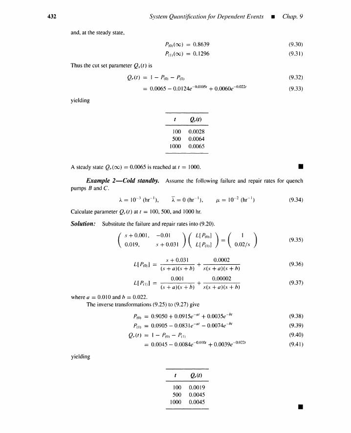
432 System Quantification/or Dependent Events _ Chap. 9
and, at the steady state,
p«»(oo) = 0.8639
p(1)(oo) = 0.1296
Thus the cut set parameter Qs(t) is
Qr(t) = 1 - p(O) - p(l)
= 0.0065 - 0.0 124e-0.()1 051 + 0.0060e -0.0221
yielding
100 0.0028500 0.0064
1000 0.0065
A steady state Qr (00) = 0.0065 is reached at t = 1000.
(9.30)
(9.31)
(9.32)
(9.33)
•Example 2-Cold standby. Assume the following failure and repair rates for quench
pumps Band C.
(9.34)
Calculate parameter Qr(t) at t = 100,500, and 1000 hr.
Solution: Substitute the failure and repair rates into (9.20).
(S+ O.OOI , -0.01 )(L[P(O)]) ( 1 )0.019, s + 0.031 L[P(l)] = 0.021s
s + 0.031 0.0002L[P(o)] = + -----
(s + a)(s + h) s(s + a)(s + h)
0.001 0.00002L[P(l)] = + -----
(s + a)(s + h) s(s + a)(s + h)
where a = 0.010 and h = 0.022.The inverse transformations (9.25) to (9.27) give
P(o) = 0.9050 + 0.0915e-a 1 + 0.0035e-h1
p(1) = 0.0905 - 0.0831e-a1- 0.0074e-h1
Qr(t) = 1 - p(m - p(1)
= 0.0045 - 0.0084e-0.0101+ 0.003ge-0.0221
yielding
100 0.0019500 0.0045
1000 0.0045
(9.35)
(9.36)
(9.37)
(9.38)
(9.39)
(9.40)
(9.41)
•

Sec.9.2 • Markov Modelfor Standby Redundancy 433
Example 3-Hot standby. Let quench pumps A and B have the failure and the repair rates
A= I = 10-3 (hr"), JL = 10-2 (hr") (9.42)
Calculate Qr (t) at t = 100, 500, and 1000 hr.
Solution: In this case, pumps Band C are statisticallyindependentand we calculate Qr(t) withoutsolving differential equation (9.16).
From Table 6.10,
Thus
Q(t) = unavailabilityof pump B
= unavailabilityof pump CA= --(1 - e-(A+/t)t)
A+JL
(9.43)
Therefore
= (_A_)2 _2 (_A_)2 e-().+Il)1 + (_A_)2 e-2().+Il)1 (9.45)A+JL A+JL A+JL
= 0.0083 - 0.0165e-O•01 1t + 0.0083e-o.022t (9.46)
Qr(t)
100 0.0037500 0.0082
1000 0.0083
Table 9.1 summarizes the results of Examples 1 to 3. As expected,
unavailabilityof hot standby> unavailabilityof warm standby> unavailabilityof cold standby
TABLE 9.1. Summary of Examples 1 to 3
Example 1 Example 2 Example 3Warm Cold Hot
Qr(100) 0.0028 0.0019 0.0037Qr(500) 0.0064 0.0045 0.0082Qr(IOOO) 0.0065 0.0045 0.0083
A 0.001 0.001 0.001I 0.0005 0 0.001
JL 0.01 0.01 0.01
(9.47)
•Example 4-Tail-gas system unavailability. Consider the tail-gasquench clean-up sys-
tem of Figure 8.12. Assume the failure and repair rates in Example 1 for the quench pumps (warmstandby); the rates in Example 2 for the circulation pumps (cold standby); and the following rates for

434 System Quantification for Dependent Events _ Chap. 9
booster fan A, feed pump D, and filter G:
A* = 10- 4,
Evaluate the system unavailability Q.\' (t) at t = 100, 500, and 1000 hr.
Solution: From Examples I and 2, we have
Q;(/) = Pr{BnC} Q;'(/) = Pr {EnF}
(9.48)
and,
100500
1000
0.00280.00640.0065
0.00190.00450.0045
Thus
Q*(t) = Pr{A} = Pr{D} = PrIG}A*
= ---(I - e-o.*+/L*)l)A* + /l*
= 0.0099[ I - e-O.01011]
Q*(/)
100 0.0063500 0.0098
1000 0.0099
(9.49)
Equations (9.2) and (9.4) become
Qs(t)max = 3Q*(t) + Q~(t) + Q~(t)
Qs(t)min = Qs(t)max - 3Q*(t)2 - 3Q*(t)Q~(t) - 3Q*(t)Q~(t) - Q~(t)Q~(t)
yielding
100 0.025 0.025500 0.040 0.040
1000 0.041 0.040
(9.50)
•9.2.3.2 Three-component redundancy. So far we havetreated standby redundancy
with two components. Let us now consider the tail-gas quench and clean-up system ofFigure 9.3, which has a two-out-of-three quench-pump system. Assume that each pumphas failure rate Awhen it is operating and failure rate I when it is in standby, and that onlyone pump at a time can be repaired. Note that two or less pumps are repaired at a time inFigure 9.1. Possible state transitions are shown in Figure 9.4. State I means that pumpA is in standby and pumps D and B are principal (working). State 13 shows that pumpsA, D, and B are under repair, but only pump A is currently being repaired. Transitionfrom state 7 to 13 occurs when pump B fails; it is assumed that pump B is still operatingin state 7 and rate A is used, although the two-out-of-three system is failed in this state;
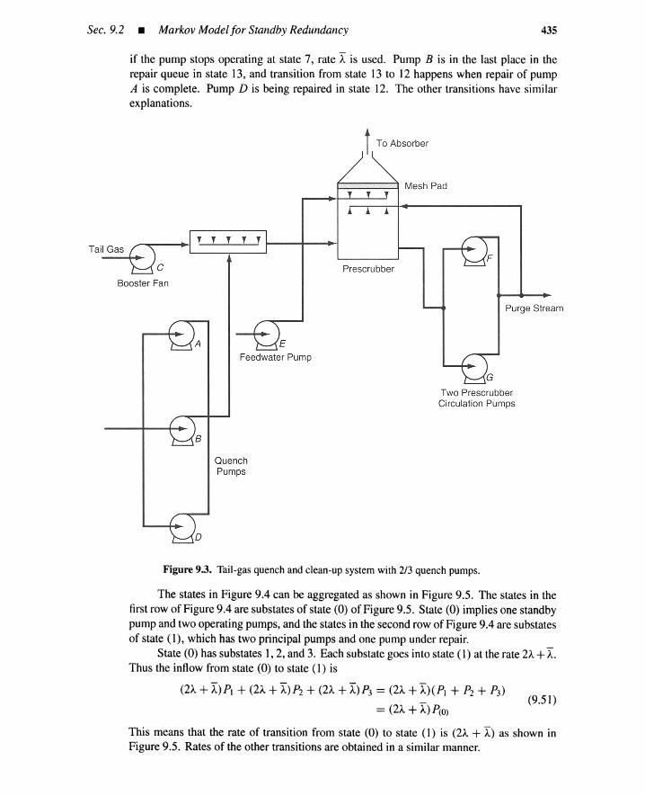
Sec. 9.2 • Markov Modelfor Standby Redundancy 435
if the pump stops operating at state 7, rate I is used. Pump B is in the last place in therepair queue in state 13, and transition from state 13 to 12 happens when repair of pumpA is complete. Pump D is being repaired in state 12. The other transitions have similarexplanations.
!==:::::::==~ Mesh Pad
Tail Gas,..--.:--_ -.j T T T T T ~_-+__~I
Prescrubber
Booster Fan
Purge Stream
E
Feedwater Pump
Two PrescrubberCirculation Pumps
B
QuenchPumps
o
Figure 9.3. Tail-gas quench and clean-up system with 2/3 quench pumps .
(9.51)
The states in Figure 9.4 can be aggregated as shown in Figure 9.5. The states in thefirst row of Figure 9.4 are substates of state (0) of Figure 9.5. State (0) implies one standbypump and two operating pumps, and the states in the second row of Figure 9.4 are substatesof state (I), which has two principal pumps and one pump under repair.
State (0) has substates I, 2, and 3. Each substate goes into state (I) at the rate 2A+I.Thus the inflow from state (0) to state ( I) is
(2), +I)p, + (2), +I )P2+ (2), +I)P3 = (2A+I)(P1 + P2 + P3)
= (2), + I)p(o)
This means that the rate of transition from state (0) to state (I) is (2)"+ I ) as shown inFigure 9.5. Rates of the other transitions are obtained in a similar manner.
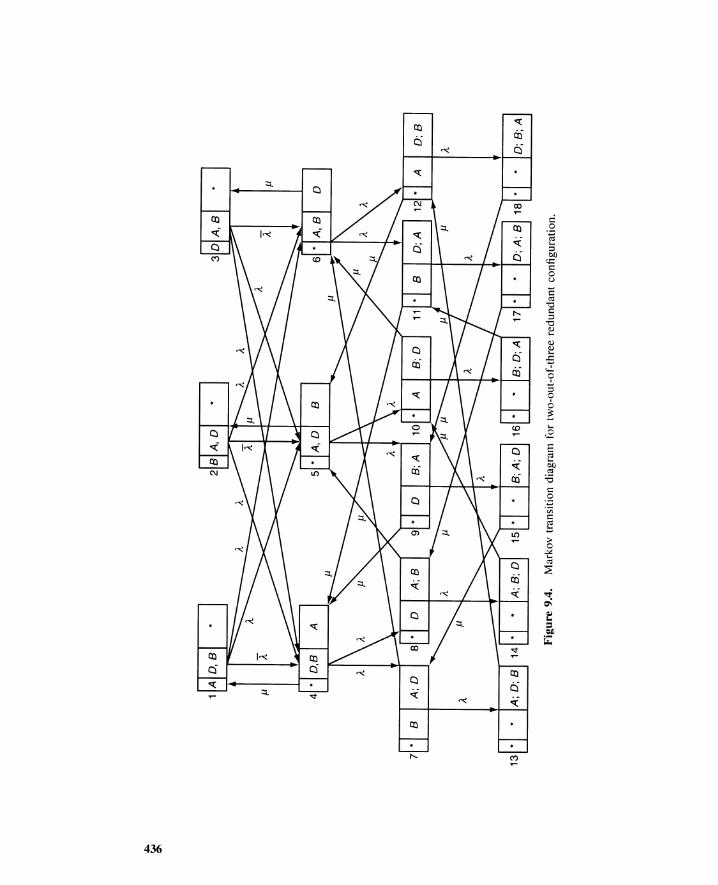
~ ~ ~
71*
1B
Fig
ure
9.4.
Mar
kov
tran
siti
ondi
agra
mfo
rtw
o-ou
t-of
-thr
eere
dund
ant
conf
igur
atio
n.
D;B
A D;B
;A
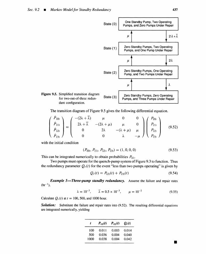
Sec.9.2 • Markov Modelfor Standby Redundancy
State (0)
State (1 )
State (2)
Figure 9.5. Simplified transition diagramfor two-out-of-three redun- State (3)dant configuration.
437
One StandbyPump, Two OperatingPumps, and Zero PumpsUnderRepair
~
J1 2A+I"
Zero StandbyPumps, Two OperatingPumps, and One PumpUnderRepair
J1 2A
Zero StandbyPumps, One OperatingPump, and Two PumpsUnderRepair
~~
J1 A"
Zero StandbyPumps, Zero OperatingPumps, and Three PumpsUnderRepair
The transition diagram of Figure 9.5 gives the following differential equation.
p(O)
PO)
P(2)
P(3)
=
-(2A + I)2,,-+I
oo
Jl
-(2A + Jl)
2"-
o
(9.52)
with the initial condition
(9.53)
This can be integrated numerically to obtain probabilities Pu).Two pumps must operate for the quench-pump system of Figure 9.3 to function. Thus
the redundancy parameter Qr(t) for the event "less than two pumps operating" is given by
(9.54)
Example 5-Three-pump standby redundancy. Assume the failure and repair rates(hr- 1),
- -3A= 0.5 x 10 , J1; = 10- 2 (9.55)
Calculate Qr(t) at t = 100,500, and 1000 hour.
Solution: Substitute the failure and repair rates into (9.52). The resulting differential equationsare integrated numerically, yielding
P(2)(t) P(3)(t) Qr(t)
100 0.011 0.003 0.014500 0.036 0.004 0.040
1000 0.038 0.004 0.042 •
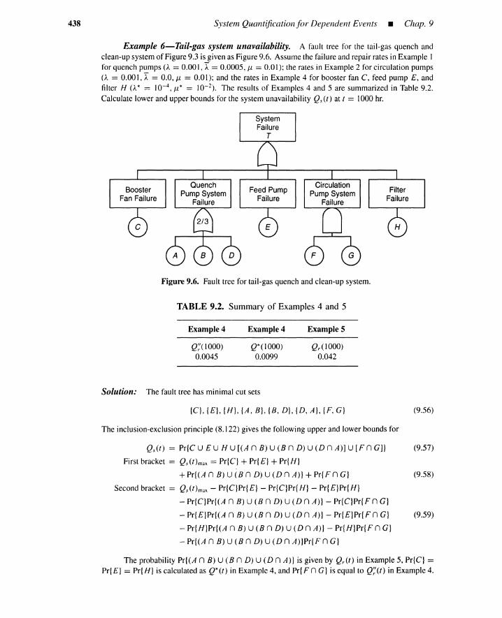
438 System Quantification for Dependent Events _ Chap. 9
Example 6-Tail-gas system unavailability. A fault tree for the tail-gas quench andclean-up system of Figure9.3 is givenas Figure9.6. Assume the failureand repair rates in Example Ifor quench pumps (A = 0.00 I, I = 0.0005, J1 = 0.0 I); the rates in Example 2 for circulation pumps(A = 0.001, I. = 0.0, J1 = 0.01); and the rates in Example 4 for booster fan C, feed pump E, andfiIter H (A* = 10- 4
, J1 * = 10- 2) . The results of Examples 4 and 5 are summarized in Table 9.2.Calculate lower and upper bounds for the system unavailability Q.,.(t) at t = 1000hr.
SystemFailure
T
BoosterFan Failure
QuenchPump System
Failure
Feed PumpFailure
CirculationPump System
Failure
FilterFailure
Figure 9.6. Fault tree for tail-gas quench and clean-up system.
TABLE 9.2. Summary of Examples 4 and 5
Example 4
Q;:( 1000)0.0045
Example 4
Q*(IOOO)0.0099
Example 5
Qr( 1000)0.042
Solution: The fault tree has minimal cut sets
{C}, {E}, {H}, {A, B}, {B, D}, {D, A}, {F, G}
The inclusion-exclusionprinciple (8.122) gives the following upper and lower bounds for
(9.56)
Qs(t) = Pr{C U E U H U [(A n B) U (B n D) U (D n A)] U [Fn G]} (9.57)
First bracket = Qs(t)max == Pr{C} + Pr{ E} + Pr{ H}
+Pr{(A n B) U (B n D) U (D n A)} + Pr{Fn G} (9.58)
Second bracket = Qs(t)max - Pr{C}Pr{E} - Pr{C}Pr{H} - Pr{E}Pr{H}
- Pr{C}Pr{(A n B) U (B n D) U (D n A)} - Pr{C}Pr{ F n G}
- Pr{ E}Pr{(A n B) U (B n D) U (D n A)} - Pr{ E}Pr{ F n G} (9.59)
- Pr{ H}Pr{(A n B) U (B n D) U (D n A)} - Pr{H}Pr{ F n G}
- Pr{(A n B) U (B n D) U (D n A)}Pr{F n G)
The probability Pr{(A n B) U (B n D) U (D n A)} is given by Qr(t) in Example 5, Pr{C} =Pr{ E} = Pr{ H} is calculated as Q*(t) in Example 4, and Pr{ F n G} is equal to Q~(t) in Example 4.

Sec.9.2 • Markov Modelfor Standby Redundancy
Thus
439
Qs(t)max = 3Q*(t) + Qr(t) + Q~ (t)
= 3 x 0.0099 + 0.042 + 0.0045 = 0.076
Qs(t)min = 0.076 - 3Q*(t)2 - 3Q*(t)Qr(t) - 3Q*(t)Q~(t) - Qr(t)Q~(t) (9.60)
= 0.076 - 0.0003 - 0.0013 - 0.0001 - 0.0002
= 0.074
and the system unavailability is bracketedby
0.074 :s Qs(t) s 0.076 (9.61)
•9.2.3.3 n-Component redundancy. As a general case, consider standby redundan-
cies satisfying the following requirements.
1. The standby redundancy consists of n identical components.
2. The redundant configuration has m (::s n) principal components.
3. At most, r (::: 1) components can be repaired at a time.
An aggregated transition diagram is shown in Figure 9.7, and we have the differentialequations
p(O) = -AOP(O) + ~lP(l)
(9.62)
(9.63)
where k - number of components under repairAk == m): + (n - m - k)I, for k = 0, , n - mAk == (n - k)A, for k = n - m + 1, , n - 1~k == min{r, k} sc u; for k = 1, ... , n
The parameter Qr(t) is given by
Qr(t) = p(n-m+l)(t) + ... + p(n)(t) (9.64)
Equation (9.12) is a special case of (9.62), where n = 2, m = 1, and r = 2. Similarly,equation (9.52) is obtained from (9.62) by setting n = 3, m = 2, and r = 1.
9.2.4 Steady-State Unavailability
The steady-state solution of (9.62) satisfies
o= -AOP(O) + ~l PO)
(9.65)
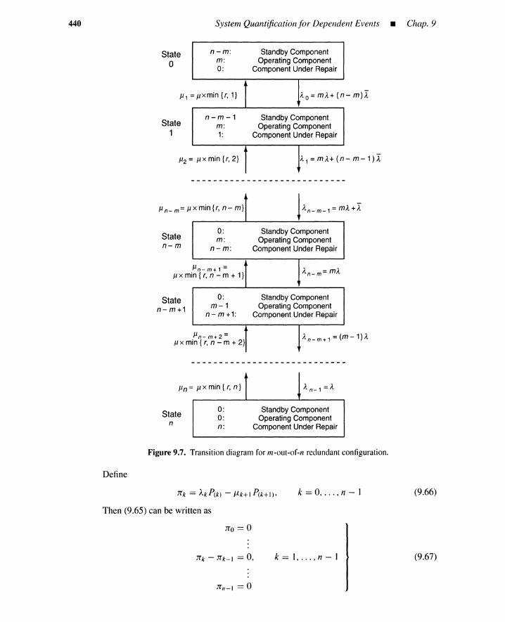
440 System Quantification for Dependent Events _ Chap. 9
Stateo
State1
n-m: Standby Componentm: Operating Component0: Component Under Repair
= J.1xmin {r, 1} Ao=mA+(n
n-m -1 Standby Componentm: Operating Component1: Component Under Repair
u x min {r, 2} A1=mA+(n,~
-m-1)):
m-1)A
~~
!A n _ m _ 1 = mxmin{r,n-m}
0: Standby Componentm: Operating Component
n-m: Component Under Repair
J.1 n - m» 1 = An - m= m):in { r, n - m + 1} ,
0: Standby Componentm-1 Operating Component
n-m+1: Component Under Repair
J.1 n - m +2 = !A n - m + 1 = (in { r, n - m + 2}
J.1xm
J.1xm
Staten-m
J.1 n - m=J.1
Staten- m+1
Iln= Il x min {r, n}IState
n
0:0:n:
Standby ComponentOperating Component
Component Under Repair
Figure 9.7. Transition diagram for nl-out-of-n redundantconfiguration.
Define
JTk == AkP(k) - JLk+l P(k+l),
Then (9.65) can be written as
k == 0, ... , n - 1 (9.66)
JTo == 0
JTk - JTk-l == 0, k==l, ... ,n-l (9.67)
Jrl1 - 1 == 0
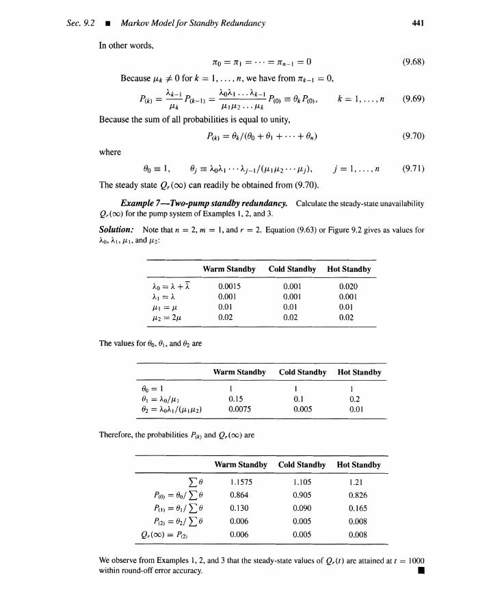
Sec. 9.2 • Markov Model for Standby Redundancy
In other words,
JTo == JTl == ... == JTn-l == 0
Because ~k f 0 for k == 1, ... , n, we have from JTk-l == 0,
Ak-l AOAI ... Ak-lP(k) == --P(k-l) == P(O) =OkP(O), k == 1, ... , n
~k ~1J.-l2·· ·J.-lk
Because the sum of all probabilities is equal to unity,
P(k) == Ok/(OO + OJ + ... + On)
where
00=1, OJ=AOAJ···Aj-l/(~1~2···~j), j==I, ... ,n
The steady state Qr(oo) can readily be obtained from (9.70).
441
(9.68)
(9.69)
(9.70)
(9.71)
Example 7-Two-pump standby redundancy. Calculate the steady-state unavailabilityQr (00) for the pump system of Examples 1, 2, and 3.
Solution: Note that n = 2, m = 1, and r = 2. Equation (9.63) or Figure 9.2 gives as values forAo, A}, J.LJ, and J.L2:
Warm Standby Cold Standby Hot Standby
AQ = A+I 0.0015 0.001 0.020
Al =A 0.001 0.001 0.001
J.LI =J.L 0.01 0.01 0.01
J.L2 = 2J.L 0.02 0.02 0.02
The values for eo,eI , and e2 are
Warm Standby Cold Standby Hot Standby
eo = 1 1 1 1(h = AolJ.Ll 0.15 0.1 0.2e2 = AoAl/(J.LIJ.L2) 0.0075 0.005 0.01
Therefore, the probabilities P(k) and Qr(oo) are
Warm Standby Cold Standby Hot Standby
L(J 1.1575 1.105 1.21
P(O) = eol L () 0.864 0.905 0.826
PO) ~ ell L(J 0.130 0.090 0.165
P(2) = e21L o 0.006 0.005 0.008
Qr(OO) = P(2) 0.006 0.005 0.008
We observe from Examples 1, 2, and 3 that the steady-state values of Qr (t) are attained at t = 1000within round-off error accuracy. •

442 System Quantificationfor Dependent Events _ Chap. 9
Example 8-Three-pump standby redundancy. Consider the pumping system of Ex-ample 5. Calculate the steady-state Qr(oo) for the event "less than two pumps operating."
Solution: We note that n = 3, m = 2, and r = 1. Equation (9.52) or Figure 9.5 gives
Values of fh are
An = 2A+ X= 0.0025,Al = 2A = 0.002,A2 = A = 0.001,
Jll = Jl = 0.01Jl2 = Jl = 0.01Jl3 = Jl = 0.01
(9.72)
Equation (9.70) gives
eo = 1
el = AolJll = 0.25
fh = AnAI/(JlIJl2) = 0.05
e3 = AOAIA2/(JlIJl2Jl3) = 0.005
2: 8 p(O) =80 / 2: 8 P(l) =81I 2: (J P(2) =821 2: (J p(J) =(JJI 2: 8
1.305 0.766 0.192 0.038 0.004
Hence from (9.54)
Qr(OO) = 0.038 + 0.004 = 0.042
This steady-state value confirms Qr(t) at t = 1000, as in Example 5.
9.2.5 Failures per Unit Time
(9.73)
(9.74)
•9.2.5.1 Two-component redundancy. The parameter ws(t) is important in that its
integration over a time interval is the expected number of system failures during the interval.As shown by (8.194) and (8.195), an upper bound for ui, (t) is
m
ws(t)max == L w7(t);=1
Consider the fault tree of Figure 8.13 that has five minimal cut sets:
(9.75)
d, == {A} dJ == {G} d4 == {B, C} ds == {E, F} (9.76)
(9.78)
Equation (9.75) becomes
ws(t)max == w;(t) + w~(t) + wi(t) + w;(t) + w;(t) (9.77)
For cut set {B, C} to fail, either one of Band C should fail in t to t + dt with theother remaining basic event already existing at time t. Thus w:(t)dt is
w:(t)dt == Pr{B fails during [t, t+dt)IBnC at time t}Pr{BnC at time t}
+Pr{C fails during [t, t +dt)IBnC at time t}Pr{BnC at time t}
Assume failure rate 'A' for pumps Band C. Then
w;(t)dt == 'A'dt x [Pr{Bn C at time t} + Pr{B neat time tl]
== 'A'dt . P(l)(t)(9.79)

Sec.9.2 • Markov Modelfor Standby Redundancy 443
where p(l)(t) is the probability of one failed pump existing at time t, and is given by thesolution of (9.12). Similarly,
(9.80)
(9.81)
where A" failure rate for pumps E and F,P[i)(t) == probability of either pump E or F, but not both, being failed at time t
Thus the upper bound ws(t) can be calculated by
ws(t)max == Al[I - QI (t)] + A2[] - Q2(t)] + A3[1 - Q3(t)]
+ A'p(l) (t) + A"P(2) (t)
Example 9-Tail-gas system configuration 1. Calculate ws(IOOO)max for Figure 8.12using the failure and repair rates of Example4.
Solution: We have, from Example 4,
Al = A2 =A3 =A* = 10- 4
J.lI = J.lz = J.l3 = J.l* = 10-3
QI(t) = Qz(t) = Q3(t) = _A_*- [I - e-()..*+J.L*)t]. A* + J.l*
= 0.0099 at t = 1000
A' = A"=A=10-3
Using (9.29) and (9.39),
P(J) = 0.1296 - 0.1 I7ge-at - 0.0117e-bt
= 0.130 at t = 1000, warm standby
P(~) = 0.0905 - 0.083 Ie-at - 0.0074e-bt
= 0.090 at t = 1000, cold standby
Substituting these values into (9.81),
ws(lOOO)max = 3 x 10⁻⁴ x [I - 0.0099] + 10-3 x 0.130 + 10-3 x 0.090= 0.00052 times/hr
The MTBF is approximatedby
MTBF = 1/0.00052 hr = 80 days
(9.82)
(9.83)
(9.84)
(9.85)
(9.86)
(9.87)
(9.88)
(9.89)
•9.2.5.2 Three-component redundancy. Next consider the fault tree of Figure 9.6
that has seven minimal cut sets:
dl=={C},
d5 == {B, D},
d2 == {E}, d3 == {H}, d4 == {A, B}
d6 == {D, A}, d7 == {F, G}(9.90)
Denote by wr(t) the expected number of times that the quench-pump system fails perunit time at time t. Then, similarly to (9.75), we have as an upper bound
(9.91)
For the redundant system to fail in time t to t + dt, one pump must fail during [t, t + dt)with the redundant system already in state (1) of Figure 9.5. The rate of transition from

444 System Quantification for Dependent Events _ Chap. 9
state (1) to (2) is 2A. Thus
W,.(t) == 2)" . P(I) (t) (9.92)
where P(l)(t) is the probability that the redundant system has one failed pump at time t , asgiven by (9.52).
Example lO-Tail-gas system configuration 2. Calculate ws(t)max at t = 1000 usingthe failure and repair rates of Example 6.
Solution: Parameter ui, (t) is given by
wr(t) = 2 X 10- 3X p(l)( 1000) = 2 X 10- 3 x 0.19 = 0.00038 (9.93)
because numerical integration of (9.52) yields
P(l)(IOOO) = 0.19
From the results of Example 9 for w~(t) = lJJ;(t) == w;(t) and w~(t),
ws(t)max = 3 x 10- 4 x [I - 0.0099] + 0.00038 + 10- 3 x 0.090
= 0.00077
The MTBF is approximated by
MTBF = 1/0.00077 hr = 54 days
(9.94)
(9.95)
(9.96)
•9.2.5.3 n-Component redundancy. As a general case, consider an m-out-of-n re-
dundant configuration with r repair crews. Let a fault tree havecut sets that include compo-nent failures in the redundancy. The calculation of ws(t)max is reduced to evaluating W,.(t),
defined as
WI' (t) == the expected number of times that the redundant configuration fails perunit time at time t
== mAP(n-m)(t)
where p(n-m)(t) == the probability of (n - m) components being failed at time t
== the probability of state (n - m) in Figure 9.7m A == the rate of transition from state (n - m) to (n - m + 1)
9.2.6 Reliability and Repairability
As a first step, we partition the set of all states into operational states (U: up) andfailed states (D: down). For the m-out-of-n configurationof Figure 9.7, states 0, ... , n - m
are operational and states n - m + I, ... , n are failed. For each state S, we write S E Uwhen the system is operational and SED when the system is failed. System reliabilityR(t), availability A(t), and repairability M(t) are defined by [2]
R(t) == Pr{S E U during (0, t]IS(E U) at time O}
A(t) == Pr{S E U at time tIS(E U U D) at time O}
M(t) == I - Pr{S E D during (0, t]IS(E D) at time O}
(9.97)
(9.98)
(9.99)
The system availability is calculated by solving differential equations such as (9.62).To calculate the system reliability, the transition diagram of Figure 9.7 is modified in thefollowing way.
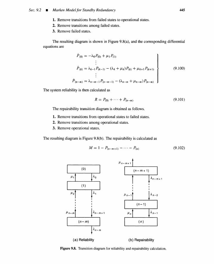
Sec. 9.2 • Markov Mode/for Standby Redundancy
1. Remove transitions from failed states to operational states.
2. Remove transitions among failed states.
3. Remove failed states.
445
The resulting diagram is shown in Figure 9.8(a), and the corresponding differentialequations are
p(o) == -AOP(O) + J-ll P(l)
The system reliability is then calculated as
R == p(O) + ... + p(n-m)
The repairability transition diagram is obtained as follows.
1. Remove transitions from operational states to failed states.
2. Remove transitions among operational states.
3. Remove operational states.
The resulting diagram is Figure 9.8(b). The repairability is calculated as
M == 1 - p(n-m+1) - ... - p(n)
(9.100)
(9.101)
(9.102)
(a) Reliability (b) Repairability
Figure 9.8. Transition diagram for reliability and repairability calculation.
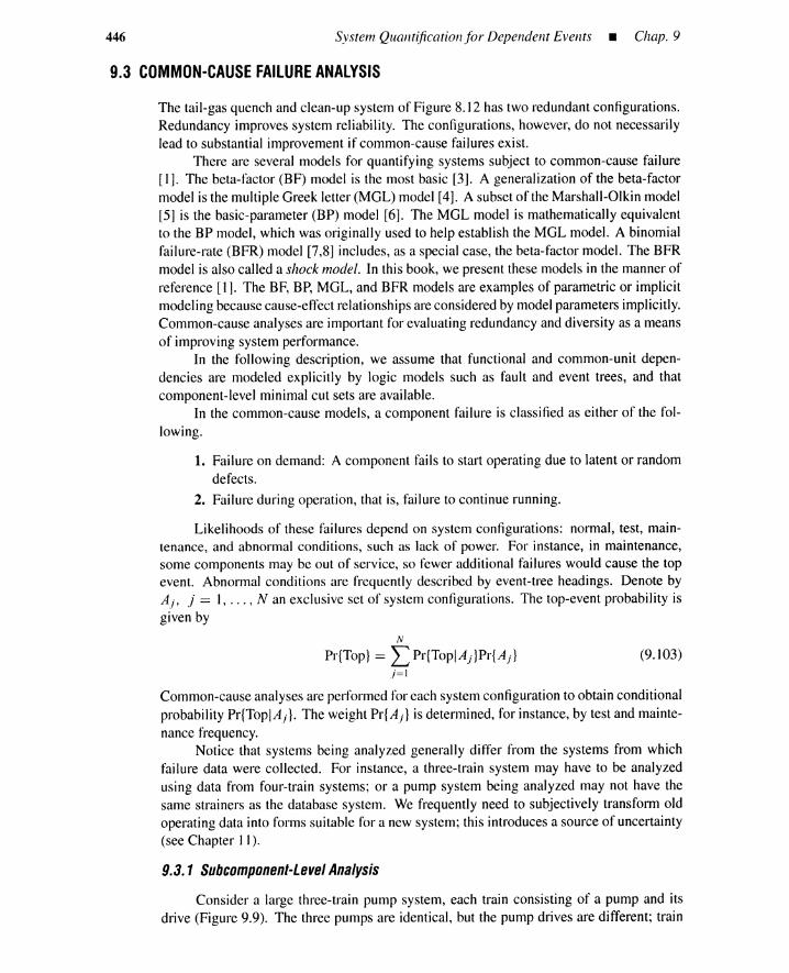
446 System Quantification for Dependent Events _ Chap. 9
(9.103)
9.3 COMMON-CAUSE FAILURE ANALYSIS
The tail-gas quench and clean-up system of Figure 8.12 has two redundant configurations.Redundancy improves system reliability. The configurations, however, do not necessarilylead to substantial improvement if common-cause failures exist.
There are several models for quantifying systems subject to common-cause failure[I]. The beta-factor (BF) model is the most basic [3]. A generalization of the beta-factormodel is the multiple Greek letter (MGL) model [4]. A subset of the Marshall-Olkin model[5] is the basic-parameter (BP) model [6]. The MGL model is mathematically equivalentto the BP model, which was originally used to help establish the MGL model. A binomialfailure-rate (BFR) model [7,8] includes, as a special case, the beta-factor model. The BFRmodel is also called a shock model. In this book, we present these models in the manner ofreference [1]. The BF, BP, MGL, and BFR models are examples of parametric or implicitmodeling becausecause-effect relationships are considered by modelparameters implicitly.Common-cause analyses are important for evaluating redundancy and diversity as a meansof improving system performance.
In the following description, we assume that functional and common-unit depen-dencies are modeled explicitly by logic models such as fault and event trees, and thatcomponent-level minimal cut sets are available.
In the common-cause models, a component failure is classified as either of the fol-lowing.
1. Failure on demand: A component fails to start operating due to latent or randomdefects.
2. Failure during operation, that is, failure to continue running.
Likelihoods of these failures depend on system configurations: normal, test, main-tenance, and abnormal conditions, such as lack of power. For instance, in maintenance,some components may be out of service, so fewer additional failures would cause the topevent. Abnormal conditions are frequently described by event-tree headings. Denote byAi- j == 1, ... , N an exclusive set of system configurations. The top-event probability isgiven by
N
Pr{Top} == L Pr{ToplA j }Pr{Aj }
j=l
Common-cause analyses are performed for each system configuration to obtain conditionalprobability Pr{TopIAj } . The weight Pr{Aj } is determined, for instance, by test and mainte-nance frequency.
Notice that systems being analyzed generally differ from the systems from whichfailure data were collected. For instance, a three-train system may have to be analyzedusing data from four-train systems; or a pump system being analyzed may not have thesame strainers as the database system. We frequently need to subjectively transform oldoperating data into forms suitable for a new system; this introduces a source of uncertainty(see Chapter I 1).
9.3.1 SUbcomponent-Level Analysis
Consider a large three-train pump system, each train consisting of a pump and itsdrive (Figure 9.9). The three pumps are identical, but the pump drives are different; train
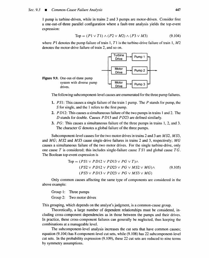
Sec. 9.3 • Common-Cause Failure Analysis 447
I pump is turbine-driven, while in trains 2 and 3 pumps are motor-driven. Consider firsta one-out-of-three parallel configuration where a fault-tree analysis yields the top-eventexpression:
Top == (PI v TI) /\ (P2 v M2) /\ (P3 v M3) (9.104)
where PI denotes the pump failure of train I, T I is the turbine-drive failure of train I, M2denotes the motor-drive failure of train 2, and so on.
Figure 9.9. One-out-of-three pumpsystem with diverse pumpdrives.
(9.105)
The following subcomponent-level causes are enumerated for the three pump failures.
1. P81: This causes a single failure of the train 1pump. The P stands for pump, the8 for single, and the I refers to the first pump.
2. P D12: This causes a simultaneous failure of the two pumps in trains I and 2. TheD stands for double. Causes P D13 and P D23 are defined similarly.
3. PG: This causes a simultaneous failure of the three pumps in trains 1,2, and 3.The character G denotes a global failure of the three pumps.
Subcomponent-level causes for the two motor drives in trains 2 and 3 are M 82, M 83,and MG; M82 and M83 cause single-drive failures in trains 2 and 3, respectively; MGcauses a simultaneous failure of the two motor drives. For the single turbine-drive, onlyone cause T is considered; this includes single-failure cause T 81 and global cause TG.The Boolean top-event expression is
Top == (PSI v PDI2 v PDI3 v PG v T)/\
(PS2 v P DI2 v P D23 v PG v MS2 v MG)/\
(PS3 v PDI3 v PD23 v PG v MS3 v MG)
Only common causes affecting the same type of components are considered in theabove example:
Group 1: Three pumps
Group 2: Two motor drives
This grouping, which depends on the analyst's judgment, is a common-cause group.Theoretically, a large number of dependent relationships must be considered, in-
cluding cross-component dependencies as in those between the pumps and their drives.In practice, these cross-component failures can generally be neglected, thus keeping thecombinations at a manageable level.
The subcomponent-level analysis increases the cut sets that have common causes;equation (9.104) has 8 component-level cut sets, while (9.108) has 22 subcomponent-levelcut sets. In the probability expression (9.109), these 22 cut sets are reduced to nine termsby symmetry assumptions.

448 System Quantification for Dependent Events _ Chap. 9
Consider a consensus operation, described in Chapter 5. The operation with respectto biform variable Y; in (8.107) yields the consensus lj;(l i , Y) /\ lj;(0;, Y). Because functionlj; (Y) is monotonically increasing, this consensus simplifies to lj; (0;, Y), and the followingexpansion holds.
(9.106)
(9.107)
(9.109)
Consider a sequence of biform variables PG, P D 12, P D23, P D 13, and MG. Byrepeated applications of (9.106), (9.105) can be expanded in the following way:
Top == PG v PDI2(PS3 v PD13 v PD23 v MS3 v MG)v
PD23(PSI v PD13 v T) v PD13(PS2 v MS2 v MG)v
MG(PSI v T)v
(PSI + T)(PS2 + MS2)(PS3 + MS3)
This can be arranged as
Top == PG v (PD12PD13 v PD12PD23 v PDI3PD23)v
(PDI2PS3 v PD23PSI v PDI3PS2) v (PDI2MG v PDI3MG)v(9.108)
(PDI2MS3 v PDI3MS2) v PD23T v MGT v MGPSlv
(PSI + T)(PS2 + MS2)(PS3 + MS3)
The last term represents the pure single-failure contribution.All subcomponent-level causes are mutually independent. Because of the symmetry
within a common-cause group of components (i.e., a group of pumps or a group of motordrives), we have the probability expression
Pr{Top} ~ P..1 + 3P} + 3P2PI + 2P2M2 + 2P2MI + P2T + M2T
+ M 2PI + (PI + T)(P} + MI )2
P3 denotes the triple-failure probability of three pumps at the same time, P2 the double-failure probability of pumps 1 and 2 (with pump 3 normal), and so on. Note that P2 isalso a failure probability of pumps I and 3 (or pumps 2 and 3). In other words, Pj is thesimultaneous-failure probability within a particular group of j pumps, while the pumpsoutside the group are normal.
To obtain the top-event probability, we first calculate the following quantities usingthe models described in the following sections.
P.1' P2, PI: for the 3 pumps
M2, M1: for the 2 motor-drives
T: for the single turbine drive
(9.110)
(9.111)
(9.112)
It is noted that, prior to the application of common-cause models, top-event expres-sions are obtained in terms of the following.
1. Component failures by component-level fault trees, reliability block diagrams,Boolean expressions, and so forth. Equation (9.104) is an example.
2. Subcomponent level of causes [eq. (9.105)].
3. Boolean reduction of subcomponent-level expression [eq. (9.108)].
4. Top-eventprobability expression in terms of combinations of simultaneous failures[eq. (9.109)].
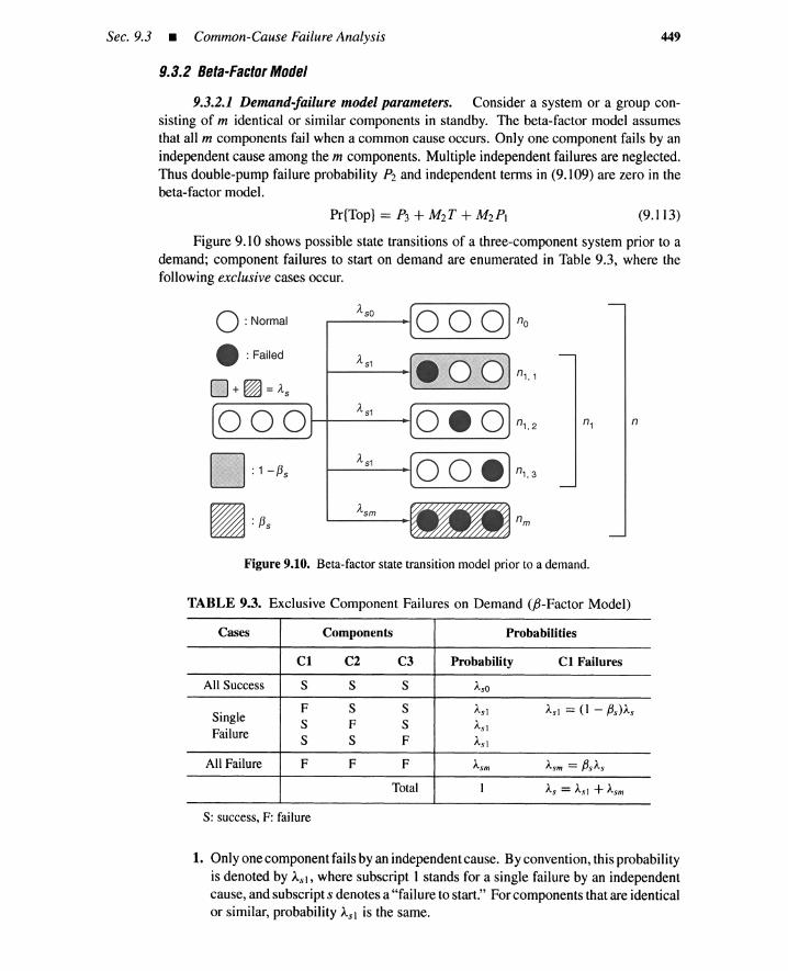
Sec. 9.3 • Common-Cause Failure Ana lysis
9.3.2 Beta-Factor Model
449
9.3.2.1 Demand-failure model parameters. Consider a system or a group con-sisting of m identical or similar components in standby. The beta-factor model assumesthat all m components fail when a common cause occurs. Only one component fails by anindependent cause among the m components. Multiple independent failures are neglected .Thus double-pump failure probability P2and independent terms in (9.109) are zero in thebeta-factor model.
(9.113)
Figure 9.10 shows possible state transitions of a three-component system prior to ademand; component failures to start on demand are enumerated in Table 9.3, where thefollowing exclusive cases occur.
o :NormalAso 00 0 no
e :Failed As, e o oO+ ~ = As
n" ,
000As, oeo n' ,2 n, n
D : 1 - 135
As, 00 e n' ,3
~:13sAsm_nm
Figure 9.10. Beta-factor state transition model prior to a demand.
TABLE 9.3. Exclusive Component Failures on Demand eB-Factor Model)
Cases Com pone nts Probabilities
Cl C2 C3 Probability Cl Failures
All Success S S S AsO
SingleF S S As] As] = (I - f3s) AsS F S A,,]
Failure S S F Asl
All Failure F F F Asm Asm = f3sAs
Total I As = Asl + Asm
S: success, F: failure
1. Only one component fails by an independent cause. By convention, this probabilityis denoted by A.sh where subscript I stands for a single failure by an independentcause, and subscript s denotes a "fa ilure to start ." For components that are identicalor similar, probability A.sl is the same .
450 System Quantification for Dependent Events _ Chap. 9
2. All components fail simultaneously by a common cause. This probability is de-noted by Asm' where subscript m stands for simultaneous failure of m componentsby a common cause, and subscript s, as before, denotes a failure to start.
Two or more components may fail simultaneously due to independent causes; how-ever, these cases are excluded from Table 9.3 by the rare-event assumption.
Consider a component that fails either by an independent or common cause. FromTable9.3, the conditional probability fJs of the common-cause failure,given an independent-(single-) or simultaneous-component failure, is
A,\'111fJ\· == ----
, A'\'111 + Asl
A."i == A'\'111 + A,d
(9.114)
(9.115)
Parameter A,,,, a constant common to all components, is an overall probability of componentfailure on demand due to independent and common causes. Parameter fJs denotes thefraction of the overall failure probability A,\' attributable to common-cause failures. Thus
ASI == (1 - fJs)A,\. (9.116)
Consider a one-out-of-m configurationsystem. The system-failure probability on de-mand, QI/m, is given by the rare-event assumption that neglects the independent-(single-) failure contribution.
(m ~ 2) (9.117)
Note that the demand-failure probability of a single-component system is
QI/I == A,\. (9.118)
Equation (9.1 17) shows that parameter fJs corresponds to the unavailability reductionachieved by the redundant configuration. Without the common cause (fJs == 0), proba-bility QI/m is underestimated because
QI/m == A~l, for independent case (9.119)
9.3.2.2 Data required. For a complete analysis, the following data are required(see Figure 9.10):
1. n == number of demands on a system level.
2. n I,i == number of independent demand failures for component i,
3. n 1 == number of independent failures for all components, such asm
nl == LnI.ii=1
(9.120)
4. nm == number of common-cause failures where all m components fail simultane-ously, and
5. no == number of successful responses to demands where all m components operatenormally.
9.3.2.3 Parameter estimation. The following equations hold:m
n == no+nm + Lnl,ii=1
(9.121)
Sec. 9.3 • Common-Cause Failure Analysis 451
(9.122)
Denote by AsO the component-success probability on demand. Because the events in Table9.3 are exclusive and there are m == 3 cases of single-component failures,
(9.123)
For each demand, one case in Table 9.3 applies; all components normal, one com-ponent fails, or all components fail. When probabilities AsO' Asm, and A.d are given, theprobability A of obtaining no,nm , and nl is
m
A == AnoAnm IlAnusO sm sl
;=1
== AnoAnmAn1sO sm sl
(9.124)
(9.125)
Maximum-likelihood estimators for AsO, Asm, and Asl are obtained by maximizing proba-bility A under the constraint of (9.123). A Lagrange multiplier method with the constraint(9.123) yields a maximization problem (v: Lagrange multiplier).
Maximize L == A + v(1 - AsO - Asm - mAsI)
Intermediate results are
(9.126)
(9.127)
Substituting ~sm and ~sl into constraint (9.123) and using the relation (9.122), we have
~sm == nm/n,
Parameter fJs in (9.114) is now
~sl == nl/(mn) (9.128)
A nmfJs == -----
nm + (nl/m)
The overall component-failure probability (9.115) is
A n; + (nl/m)As == - - - - -
n
(9.129)
(9.130)
Determination of fJs does not require the total number n of system-level demands; it is aratio of nm to nm + (n 1/ m), the total number of failures of a component.
9.3.2.4 Runfailure. So far we have considered failures to start on demand. Anothertype of failure-failures during operation after a successful start can be dealt with in a similarway if the number n of demands is replaced by the total system run time T; a commonmission time (t ~ T) is assumed for all systems tested. In this case, parameters such asArm and Arl become failure rates rather than probabilities, and subscript r stands for a "runfailure." Corresponding failure probabilities during mission time t of the system beinganalyzed are given by Armt and Arlt, respectively. These probabilities are a first-orderapproximation for exponential failure distributions.
1 - exp(-at) ~ at, o < at « 1 (9.131 )
Denote by Ar the overall failure rate for an operating component due to independent andcommon causes. The failure probability, QI/m, for one-out-of-m system (m ~ 2) is givenby the rare-event approximation.
(m 2: 2) (9.132)

452 System Quantification for Dependent Events _ Chap. 9
9.3.2.5 Diverse components. For dissimilar or diverse components, parameter f3sor (fJ,.) varies from component to component, and its maximum-likelihood estimator is
" nmf3s.i == ---
nm +nl.i(9.133)
In the beta-factor estimators of (9.129) and (9.133), susceptibilities of dissimilar ordiverse components to common-cause failures are reflected in the number nm of common-cause events resulting in total system failures; if diverse components are impervious tocommon causes, they yield no common-cause events. The use of different f3s,i values fordissimilar components implies a number n I,i of independent failures specific to the com-ponent. However, the component-dependent beta-factor in (9.133) for diverse componentsoffers little improvementover the component-independentbeta-factormodel. This is shownwhen weconsider diversecomponents that are similar in independent-failurecharacteristics(n 1,1 ::: n 1,2 ::: n 1,3); common-cause susceptibilities are reflected by n; in the expressionfor fJs.
9.3.2.6 Number ofdemands and system run time. Notice that n, the number ofdemands, is frequently unavailable. In this case, As is replaced by a generic databaseestimate ~s. Given ~s, the independent failure rate A,liI can be calculated from
The number n of demands is estimated by solving the equation
(9.134)
~sl == nl/(nln), i.e., (9.135)
(9.136)
When redundant configurations with different sizes are involved, average number m ofcomponents is used to replace m. Equation (9.135) cannot be used when we have no singlefailures, n 1 == O. In such a case, the following Bayes estimate is used.
Assume for A,,' 1 a beta prior distribution with parameter a and b:
A~I (1 - A,d)bp{Asll == ----
const.
The likelihood of obtaining n 1 component failures for nm demand is
A:~: (I - Asl)nm-1I 1
p{ntiAsIl == ~----const.
(9.137)
(9.138)
From Bayes theorem in the appendix of Chapter 3, a posterior distribution of A,d is
Atl +1I 1(I _ i , )b+lIm-n l
{i I} .'II 1'1.81P Asl nl ==
const.
Therefore, the posterior mean of As1 is
" a +nl + 1Asl == a + b + nm + 2
A uniform prior corresponds to zero parameter values, a == b == 0:
(9.139)
" nl + 1 .A,d == ---, I.e.,
nm + 2
nl - 2~,d + 1n==-----
A,d m(9.140)
This equation is used to estimate the number n of demands when the independent failurerate ~sl is known.
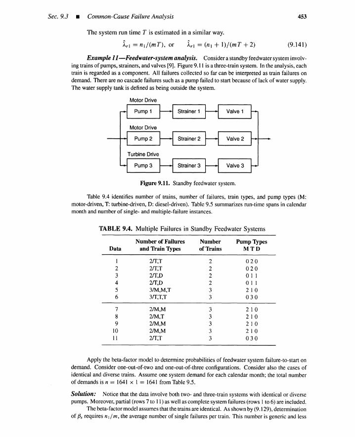
Sec. 9.3 • Common-Cause Failure Analysis
The system run time T is estimated in a similar way.
453
~rl = nl/(mT), or ~rl = (nl + l)/(mT + 2) (9.141 )
Example l l-s-Feedwater-system analysis. Considera standbyfeedwatersysteminvolv-ing trainsof pumps,strainers,and valves[9]. Figure9.11 is a three-trainsystem. In the analysis,eachtrain is regarded as a component. All failures collected so far can be interpretedas train failures ondemand. There are no cascadefailures such as a pumpfailed to start becauseof lack of water supply.The water supply tank is definedas being outside the system.
Motor Drive
Motor Drive
Turbine Drive
Figure 9.11. Standbyfeedwater system.
Table 9.4 identifies number of trains, number of failures, train types, and pump types (M:motor-driven, T: turbine-driven, 0: diesel-driven). Table9.5 summarizes run-timespans in calendarmonth and numberof single- and multiple-failure instances.
TABLE 9.4. Multiple Failures in Standby Feedwater Systems
Number of Failures Number Pump TypesData and Train Types of Trains MTD
1 2ff,T 2 0202 2ff,T 2 0203 2ff,D 2 0114 2ff,D 2 0115 3/M,M,T 3 2106 3ff,T,T 3 030
7 2/M,M 3 2108 2/M,T 3 2109 2/M,M 3 210
10 2/M,M 3 21011 2ff,T 3 030
Apply the beta-factormodel to determineprobabilities of feedwatersystem failure-to-start ondemand. Consider one-out-of-two and one-out-of-three configurations. Consider also the cases ofidenticaland diverse trains. Assumeone system demand for each calendar month; the total numberofdemandsisn = 1641 x 1 = 1641 from Table9.5.
Solution: Notice that the data involve both two- and three-train systemswith identicalor diversepumps. Moreover, partial(rows7 to 11)as wellascompletesystemfailures(rows 1to 6) are included.
The beta-factormodelassumesthatthe trainsare identical. As shownby(9.129),determinationof f3s requiresn1/m, the averagenumberof single failuresper train. This number is generic and less
454 System Quantification for Dependent Events _ Chap. 9
TABLE 9.5. Number of Failures and Run Time Spans in Calendar Months
Description
Two-train system run timeThree-train system run timeSystem run timeDiverse-train system run timeIdentical-train system run timeTrain run time
Number of single failuresNumber of common-causefailuresNumber of two-trainsystem failuresNumber of three-train system failuresNumber of diverse-train system failuresNumber of identical-train system failuresMonthly number of single failures per trainTotal number of system monthlydemandsNumber of single failures per train
Value
4741167474 + 1167 = 164113732682 x 474 + 3 x 1167 = 4449
n, = 68n; = 114 (Data 1,2,3,4)2 (Data 5, 6))3 (Data 3, 4, 5)3 (Data 1,2,6)68/4449 = 0.0153n = 1641nl/111 = 0.0153 x 1641 = 25
dependent on the number of trains /11. However, we only have a total number of single failures,n 1 = 68, during a system run time of 1641 months for systems with redundancyvaluesm = 2 and 3.The total amount of train run time is 4449 months, as calculated in the sixth row of Table 9.5. Thusthe monthly number of single failures per train is 68/4449 = 0.0153. During the run time of 1641months, 0.0153 x 1641 = 25 single failures occur per train, that is, n1/ m = 25.
The II common-cause events listed in Table 9.4 initiate the simultaneous failure of two ormore trains. When we evaluate,for a particularsystem underinvestigation, that all 11 common-causeeventswouldresult in simultaneousfailureof two trains,which is a conservativeassumption,we havenm = 11 for one-out-of-twosystems and the parameter fJs is estimated as
A 11fJ · = -- =0.3
.~ 11 + 25(9.142)
For the three-train system, only two common causes (rows 5 and 6) result in a total systemfailure. Assume that all 11 common-causeevents would result in simultaneous failure of the threetrains currently investigated. The same fJs valueas for the two-trainsystem is obtained.
Wecan also assign subjectiveweights to the partial failures due to common causes; if partialcommon-causeeventsareevaluatedas partial, thenzeroweightsare used,yieldingnm = 2+0.0 x 9 =2. The beta-factorbecomes
Bs = 2/(2 + 25) = 0.074 (9.143)
(9.144)
These weights constitute an impact vector. By using the impact vector, we can quantifycommon-causefailuresforan In-trainsystembasedonoperatingdatacollectedfor systemsofdifferentsizes.
A demand for each calendar month is assumed. A train fails 25 times by independentcausesand 11 times (a conservative estimate)by commoncausesduring the systemrun time of 1641 months.The overall demand-train-failure probability, ~s in (9.130), is
A 11 + 25As =-- = 0.022
. 1641
From (9.117), the failure probabilityof the one-out-of-two system is
Ql/2 = 0.3 x 0.022 = 6.6 x 10⁻³ (9.145)

Sec. 9.3 • Common-Cause Failure Analysis
For a one-out-of-three system
Ql/3 = 0.3 x 0.022 = 6.6 x 10-3 = Ql/2, for fJs = 0.3
Ql/3 = 0.074 x 0.022 = 1.7 x 10⁻³ < Ql/2, for fJs = 0.074
455
(9.146)
(9.147)
Table9.4 showsfour instancesof one-out-of-two systemfailures (data 1, 2, 3, and 4) during arun time of 474 months. This givesa point estimate of
Ql/2 = 4/474 = 8.4 x 10- 3
Similarly, for the three-trainsystem,
Ql/3 = 2/1167 = 1.7 x 10⁻³
(9.148)
(9.149)
As summarized in Table9.6, the beta-factormodelgivesa slightlylowerfailureprobability forthe one-out-of-two configuration than the valuesdirectlycalculatedfrom the data. The conservativebeta-factorfJs = 0.3 givesa comparatively higherfailureprobability for the one-out-of-three configu-ration,and a lessconservative beta-factor fJs = 0.074 yieldsgood agreementwith the demand-failureprobability calculatedfrom the data.
TABLE 9.6. Summary of Beta-Factor and Data Estimation
System
1/21/31/3
DiverseIdentical
0.30.30.0740.1250.428
f3-FactorModel
6.6 X 10- 3
6.6 X 10- 3
1.7 X 10- 3
2.8 X 10- 3
9.4 X 10- 3
Data
8.4 X 10⁻³
1.7 X 10⁻³
1.7 X 10⁻³
2.2 X 10- 3
11 X 10- 3
Demand-failure probabilities for diverseand identicalmultiple-train systemsare calculatedas3/1373 = 2.2 x 10- 3 and 3/268 = 11 x 10- 3, respectively (Table9.5). The numberof singlefailuresper trainfor the diverse-train systemduring 1373 monthsof run timeis n1/ m = 0.0153 x 1373 = 21,yielding fis = 3/(3 + 21) = 0.125. Similarly, nl/m = 0.0153 x 268 = 4 for the identical-trainsystem, yielding fis = 3/(3 + 4) = 0.428. Thus, Ql/m ~ 0.125 x 0.022 = 2.8 x 10- 3 for thediverse-train system (m = 2 or 3), and Ql/m ~ 0.428 x 0.022 = 9.4 x 10- 3 for identical-train system(m = 2 or 3), yieldinggood agreementwith the failure probabilities calculatedfrom the data (Table9.6). •
Example 12-Component-level analysis. The beta-factormodelcan be used at a com-ponent level, as well as on the multicomponent leveljust discussed.
Consider three components, a pump, a valve,and a strainer. From Table9.7, the beta-factorsfor pumps (fJp), valves(fJv), and strainers (fJst) are
Bp = 7/(7 + 15) = 0.32
fiv = 2/(2 + 10) = 0.17
Bst = 2/(2 + 0.3) = 0.87
For simplicityof notationthe demand-failure subscripts is not included.The overalldemand-failure probabilitiesof these componentsare
~p = (7 + 15)/1641 = 0.013
~v = (2 + 10)/1641 = 0.0073
~st = (2 + 0.3)/1641 = 0.0014
(9.150)
(9.151)
(9.152)
(9.153)
(9.154)
(9.155)

(9.156)
456 System Quantification for Dependent Events _ Chap. 9
TABLE 9.7. Data at Component Level
Single Multiple Monthly Single Single FailuresComponent Failures Failures Failures per Component per Component
Pump 40 7 40/4449 = 0.009 0.009 x 1641 = 15Valve 26 2 26/4449 = 0.006 0.006 x 1641 = 10Strainer I 2 1/4449 = 0.0002 0.0002 x 1641 = 0.3
Consider a one-out-of-two train system, where each train consists of a valve, a pump, and astrainer. Denote the two valves by I and 2. Define
1. VSl == single valve failure I, where symbol V refers to valve, S to single failure, and I tothe first valve.
2. VG == global common-cause failure of valves 1and 2.
Then the valve 1 faiIure, VI, can be represented as
Vl=VSlvVG
Similar notation is used for the two pumps and two strainers. The one-out-of-twotrain system failure,T1/ 2, is
TI/2 = (V SI v PSI v STSI v VG v PG v STG) /\
(VS2v PS2vSTS2v VGv PGvSTG)
= VGv PGvSTGv(VSI v PSI vSTSI)(VS2v PS2vSTS2)
(9.157)
(9.158)
(9.160)
By symmetry, for the failure probability of the one-out-of-two system, we have
QI/2 ~ V2+ P2 + ST2 + (VI + PI + STI)2 (9.159)
where Vj, for instance, signifies that all valveswithin a specificgroup of.i valvesfail simultaneously;.i = I for an independent cause, and .i = 2 for a common cause. The probability on the right-handside, as estimated by the beta-factor model, is
QI/2 = fJpA p + fJvAv + fJstA.'It
= 6.6 X 10-)
As expected, the final numerical result is similar to that derived earlier with the beta-factor model atthe train level [eq. (9.145)]. •
9.3.3 Basic-Parameter Model
9.3.3.1 Modelparameters. The basic-parameter(BP)model issimilar to theMarshall-Olkin model [5] except that the BP model has time-based failure rates and demand-basedfailure probabilities while the Marshall-Olkin model is strictly time based.
For a group of m components in standby, which must start and run for t hours, thereare Lm + I different parameters of the form
Asj == failure-to-start-on-demand probability for a particular group ofj components.
At) == failure-to-operate rate for a particular group of j components.t == common mission time.
In these definitions, the group is specified. For As2 , for example, components I and2 form a group, and components 2 and 3 form another group. Each group has probabil-ity Asj. Thus for a three-component system, probability of failure involving exactly two

Sec. 9.3 • Common-Cause Failure Analysis 457
components becomes 3 x As2 because there are three double-failure groups : (1,2), (1,3),(2,3). Figure 9.12 shows possible state transitions for a three-component system prior toa demand; Tables 9.8 and 9.9 show cases where component I failures are involved: onesingle failure, two double failures, and one triple failure for the three-component system ;one single failure, three double failures, three triple failures, and one quadruple failure forthe four-component system. Parameters As and numerators and denominators of {3, y, and8 listed under "coverage" are described in Section 9.3.4 .
o :Normal
• : Failed
000
n,
n
Figure 9.12. Basic-parameter state transition model prior to a demand .
TABLE 9.8. Occurrences of Component I Failure in Three-Component System
Component and Probability CoverageCl C2 C3 Probability ~ {3N {3v IN IV
F As! * *F F As2 * * * *F F As2 * * * *F F F As3 * * * * *N: numerator, D: denominator
The BP model assumes that the probability or rate of a common-cause event dependsonly on the number j of components in a group. This is a symmetry assumption. Themission time t is usually known.
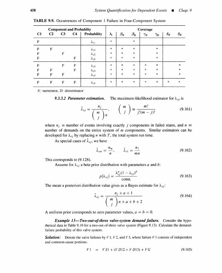
458 System Quantification for Dependent Events - Chap. 9
TABLE 9.9. Occurrences of Component 1 Failure in Four-Component System
Component and Probabilty CoverageCl C2 C3 C4 Probability As {3N {3D TN TD 6N 6D
F As1 * *F F As2 * * * *F F As2 * * * *F F As2 * * * *F F F A.d * * * * * *F F F A.d * * * * * *F F F A.d * * * * * *F F F F As4 * * * * * * *
N: numerator, D: denominator
9.3.3.2 Parameter estimation. The maximum-likelihood estimator for As} is
(9.161)(m ) m!j == j!(m - j)!is} = ( ~j) n'
where n} == number of events involving exactly j components in failed states, and n -
number of demands on the entire system of m components. Similar estimators can bedeveloped for At) by replacing n with T, the total system run time.
As special cases of ~s}, we have
" nmA.w I ==-,
n" nlAsl == -
mn(9.162)
This corresponds to (9.128).Assume for As) a beta prior distribution with parameters a and b:
A~}( 1 - As})hp{As} } == ----
const.
The mean a posteriori distribution value gives as a Bayes estimate for Asj:
" n} + a + 1As} == --------
(~ )n+a+b+2
A uniform prior corresponds to zero parameter values, a == b == O.
(9.163)
(9.164)
Example 13-Two-out-of-three valve-system demand failure. Consider the hypo-thetical data in Table 9.10 for a two-out-of-three valve system (Figure 9.13). Calculate the demand-failure probability of this valve system.
Solution: Denote the valve failures by V I, V2, and V3, where failure V 1consists of independentand common-cause portions:
VI V SI + (V DI2 + V D13) + VG (9.165)

Sec. 9.3 • Common-Cause Failure Analysis
TABLE 9.10. Data for Three-Component Valve Systems
459
Demandsn
4449
SingleFailures
nt
30
Valve 1
DoubleFailures
n2
2
TripleFailures
n3
Figure 9.13. Two-out-of-three valvesystem.
where V Sl == single failure of valve 1V D12 == double common-cause failure (CCF) of valves 1 and 2V D13 == double CCF of valves 1 and 3V G == global CCF of valves 1, 2, and 3
Similarly, we have
V2 = VS2+(VDI2+VD23)+VG
V3 = VS3+(VDI3+VD23)+VG
The simultaneous failure of valves 1 and 2 can be expressed as
VIV2 = (VSlvVDI2vVD13vVG)(VS2vVDI2vVD23vVG)
= VG v V D12 v (V SI v V D13)(V S2 v V D23)
Thus the top event V2/ 3 is
(9.166)
(9.167)
(9.168)
(9.169)
(9.170)
V2/ 3 = VIV2 v VIV3 v V2V3 (9.171)
= VG v V D12 v (V SI v V DI3)(V S2 v V D23) v VG v V D13 v
(V SI v V DI2)(V S3 v V D23) v VG v V D23 v (9.172)
(V S2 v V DI2)(V S3 v V D13)
= VG v V D12 v V D13 v V D23 v VSIVS2 v VSIVS3 v VS2VS3 (9.173)
Subcomponent-level failures are mutually independent. The probability of the top-event failure canbe approximated by the first term of the inclusion-exclusion formula.
By symmetry, for the failure probability of the two-out-of-three valve system, we have
Q2/3 == Pr{V2/ 3 } ~ V3 + 3V2 + 3V?
~ V3+3V2
(9.174)
(9.175)
where Vj denotes that j valves in a specific group fail simultaneously.The first term V3 represents a contribution by global CCF; the second term 3V2 is a contribution
by double CCF; the third term is a contribution by single failures.From the definition of Asj, the following relations hold:
(9.176)
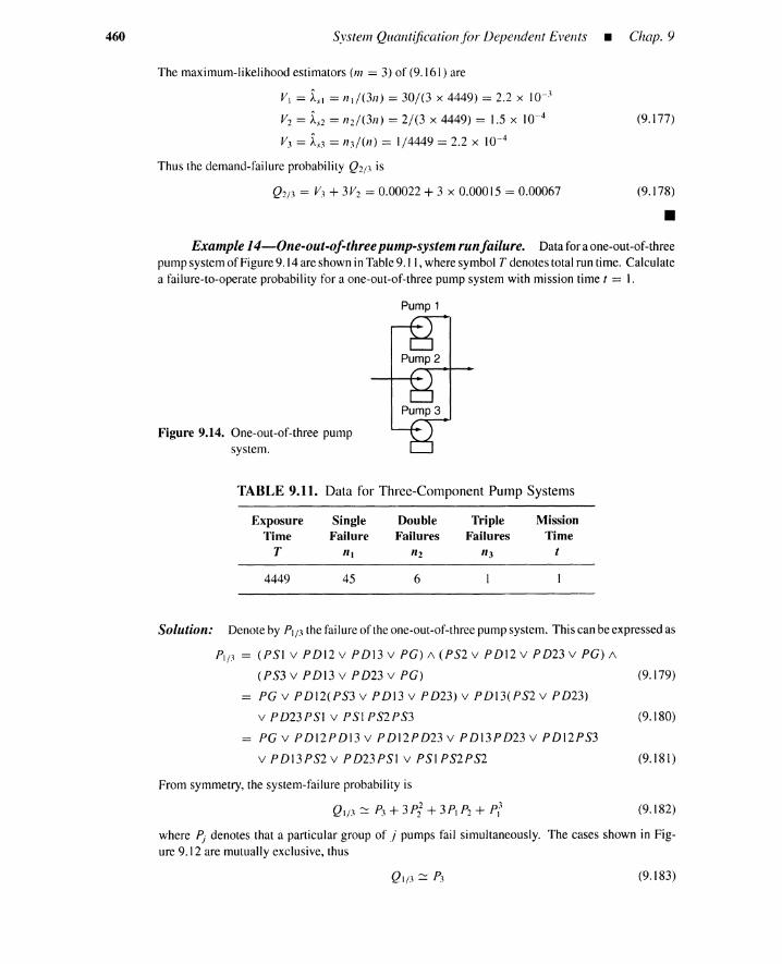
460 System Quantification for Dependent Events _ Chap. 9
The maximum-likelihood estimators (111 = 3) of (9.161) areA _~
VI = AsI = 11 I / (3/1) = 30/(3 x 4449) = 2.2 x I 0 .A 4
V2 = As2 = 112/(311) = 2/(3 x 4449) = 1.5 x lO-A -4
VJ = AsJ = I1J/(I1) = 1/4449 = 2.2 x 10
Thus the demand-failure probability Q2j3 is
Q2j3 = VJ + 3V2 = 0.00022 + 3 x 0.00015 = 0.00067
(9.177)
(9.178)
•Example 14-0ne-out-of-threepump-system runfailure. Data for a one-out-of-three
pump system of Figure 9. 14are shown in Table9.11, where symbol T denotes total run time. Calculatea failure-to-operate probability for a one-out-of-three pump system with mission time t = 1.
Pump 1
Pump 2
Pump 3
Figure 9.14. One-out-of-three pumpsystem.
TABLE 9.11. Data for Three-Component Pump Systems
Exposure Single Double Triple MissionTime Failure Failures Failures Time
T nl n2 n3 t
4449 45 6
Solution: Denote by P'/3 the failure of the one-out-of-three pump system. This can be expressed as
Pl jJ = (PSI v PDI2 v PDI3 v PC)!\ (PS2 v PD12 v PD23 v PC)!\
(PS3 v PDI3 v PD23 v PC) (9.179)
= PC v PDI2(PS3 v PDI3 v PD23) v PDI3(PS2 v PD23)
v PD23PSI v PSI PS2PS3 (9.180)
= PC v PD12PDI3 v PD12PD23 v PDI3PD23 v PDI2PS3
v P Dl3PS2 v P D23PSI v PSI PS2PS2 (9.181)
From symmetry, the system-failure probability is
QI/3::::: P.1 + 3P22 + 3PI P2 + p/' (9.182)
where P, denotes that a particular group of .ipumps fail simultaneously. The cases shown in Fig-ure 9.12 are mutually exclusive, thus
QI/3 ::::: P.1 (9.183)
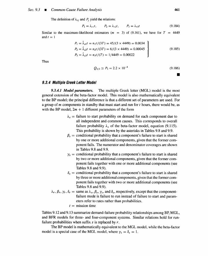
Sec. 9.3 • Common-Cause Failure Analysis
The definition of Arj and P, yield the relations:
461
(9.184)
Similar to the maximum-likelihood estimators (m = 3) of (9.161), we have for T = 4449and t = 1
Pt = ~slt = ntt/(3T) = 45/(3 x 4449) = 0.0034\
P2 = ~s2t = n2t /(3T) = 6/(3 x 4449) = 0.00045
P.1 = ~s3t = n3t / (T ) = 1/4449 = 0.00022
Thus
Ql/3 ~ P.1 = 2.2 x 10⁻⁴
9.3.4 Multiple Greek Letter Model
(9.185)
(9.186)
•9.3.4.1 Model parameters. The multiple Greek letter (MGL) model is the most
general extension of the beta-factor model. This model is also mathematically equivalentto the BP model; the principal difference is that a different set of parameters are used. Fora group of m components in standby that must start and run for t hours, there would be, aswith the BP model, 2m + 1 different parameters of the form
As = failure to start probability on demand for each component due toall independent and common causes. This corresponds to overallfailure probability As of the beta-factor model, equation (9.115).This probability is shown by the asterisks in Tables 9.8 and 9.9.
f3s = conditional probability that a component's failure to start is sharedby one or more additional components, given that the former com-ponent fails. The numerator and denominator coverages are shownin Tables 9.8 and 9.9.
Ys = conditional probability that a component's failure to start is sharedby two or more additional components, given that the former com-ponent fails together with one or more additional components (seeTables 9.8 and 9.9).
8s = conditional probability that a component's failure to start is sharedby three or more additional components, given that the former com-ponent fails together with two or more additional components (seeTables 9.8 and 9.9).
Ar, f3r, Yr, 8r = same as As, f3s, Ys, and 8s, respectively, except that the component-failure mode is failure to run instead of failure to start and param-eters refer to rates rather than probabilities.
t = mission time
Tables 9.12 and 9.13 summarize demand-failure probability relationships among BP, MGL,and BFR models for three- and four-component systems. Similar relations hold for run-failure probabilities when suffix s is replaced by r.
The BP model is mathematically equivalent to the MGL model, while the beta-factormodel is a special case of the MGL model, where Ys = 8s = 1.
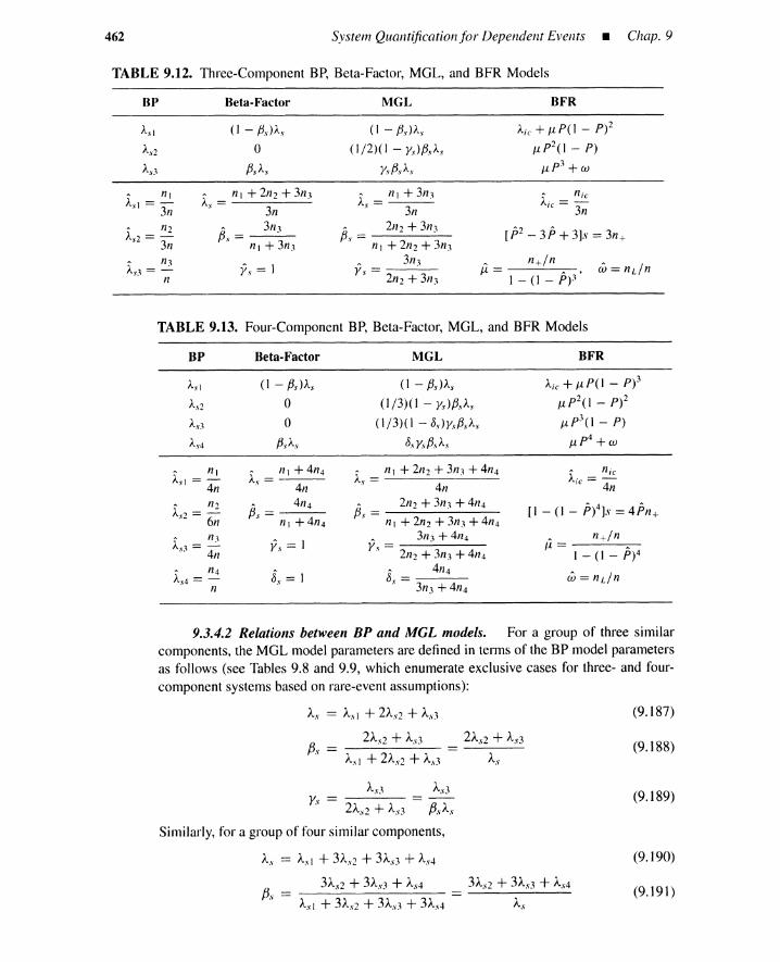
462 System Quantification for Dependent Events _ Chap. 9
TABLE 9.12. Three-Component BP, Beta-Factor, MGL, and BFR Models
BP
A nlAs l =-
311
Beta- Factor
(I - f3.JA.\.
of3sAs
nl + 2112 + 3113Xs = - - - - -
311
A 3111f3s = .
nl + 3n3
;Is = 1
MGL
(I - f3s}A s
(1/2)( I - Ys)f3.\·A.\.
Ys f3sAs
A 111 + 3113A.. =---., 3n
A 2112 + 311313\·=-----
. 111 + 2n2 + 3n3
A 3113Y\, =
. 2n2 + 3113
BFR
Aic+J1P(I- p)2
J1P2(1 - P)
J1p3 + W
A2 A[P - 3P + 3]s = 311+
A 11+111J1= A , W=I1LII1
1-(1- P)'!'
TABLE 9.13. Four-Component BP, Beta-Factor, MGL, and BFR Models
BP Beta- Factor MGL BFR
AS I (I - /3s )As (I - /3s )A.\. Aic + J1P(1 - p)3
As2 0 (l 13)(1 - Y'l) f3s As J1P2(1 _ p)2
A.d 0 (1/3)( 1 - Ds}Ysf3sAs J1P3(1 - P)
AS 4 /3sAs D.\. y\·f3sA.\. j1,p4 + W
A 111Xs =
111 + 4114X.\, =
111 + 2112 + 3113 + 4114 A l1icASI = 411
411 4nAic= -
411
A 11"Bs =
4114Bs =
2112 + 311] + 4114 A 4 A
As2 = 6~11I + 4114 111 + 2112 + 3n3 + 4114
[1-(I-P)]s=4Pn+
A 11~
;Is = 1 ;Is =3113 + 4114
,1=11+/11
As1 = --.:..1 - (I - P)4'. 411 ' 2n2 + 3113 + 4114
A 114g,\, = 1
A 4114W = I1LlnAs4 =- Ds =
11 . 3113 + 4114
9.3.4.2 Relations between BP and MGL models. For a group of three similarcomponents, the MGL model parameters are defined in terms of the BP model parametersas follows (see Tables 9.8 and 9.9, which enumerate exclusive cases for three- and four-component systems based on rare-event assumptions):
As == A.\-I + 2As2 + As3
2As2 + A.dfJs == ------
A.d + 2As2 + A,d
A,d A,dYs == ----
2As2 + A,d fJsAs
Similarly, for a group of four similar components,
A,\' == A,d + 3As2 + 3A.d + As4
{J, = 3As2 + 3A.<3 + As", A,d + 3As2 + 3As3 + 3As4
2As2 + A.d
As
3A5 2 + 3A,\"3 + As4
As
(9.187)
(9.188)
(9.189)
(9.190)
(9.191)

Sec. 9.3 • Common-Cause Failure Analysis
8 _ As4 -~s - 3As3 + 3As4 - YsfJsAs
These relations can be generalized to m-component systems.
463
(9.192)
(9.193)
(9.194)
As = t: (~ =: )Asjj=l }
1~(m-l)fJs = ;:~ i-I Asj
s ]=2
1 ~(m-l)Ys = fJ A ~ j - I As}
s s ]=3
1 ~(m-l)s, = --~. AsjYsfJsAs j=4 } - 1
The inverse relations for the BP and MGL models hold for three-component systems:
(9.195)
(9.196)
Similarly, for a four-component system,
Asl = (1 - fJs)As
As2 = (1/3)(1 - Ys)fJsAs
As3 = (1/3)(1 - 8s)YsfJsAs
As4 = 8yfJAs
9.3.4.3 Parameter estimation. Using the BP model estimators of (9.161) and(9.194), we obtain
m m
fis = Linj/Linjj=2 j=l
m m
Ys = Linj/Linjj=3 j=2
(9.197)
(9.198)
(9.199)
(9.200)m m
8s = Linj/Linjj=4 j=3
Equation (9.197) for the component overall-failure probability As coincides with(9.130) when n: = ... = nm-l = O.
A nl + mn; nm + (nl/m)As = =----
mn n(9.201)
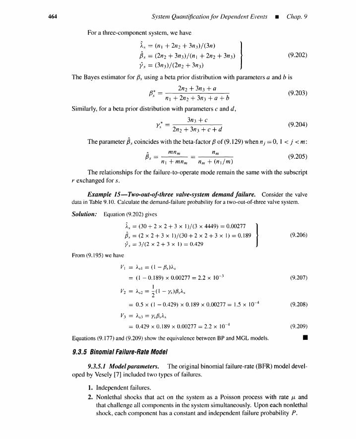
464 System Quantification for Dependent Events _ Chap. 9
For a three-component system, we have
~s == (n) + 2n2+ 3n3)/(3n) I~s == (2n2+ 3n3)/(n I + 2n2 + 3n3)
ys == (3n3) / (2n2 + 3n3)
(9.202)
(9.204)
(9.203)
(9.206)
The Bayes estimator for fJs using a beta prior distribution with parameters a and b is
* 2n2 + 3n3 + afJ,. == 2 b. n)+ n2+3n3+a+
Similarly, for a beta prior distribution with parameters c and d,
* 3n3 + cy,. ==. 2n2 + 3n3 + c + d
The parameter ~s coincides with the beta-factor fJ of (9.129) when nj == 0, 1 < j < m:
~,,== n1n m == nm (9.205). n) + mn.; nm + (n)/m)
The relationships for the failure-to-operate mode remain the same with the subscriptr exchanged for s.
Example 15-Two-out-of-three valve-system demand failure. Consider the valvedata in Table 9.10. Calculate the demand-failure probability for a two-out-of-threevalve system.
Solution: Equation (9.202) gives
~s = (30 + 2 x 2 + 3 x 1)/(3 x 4449) = 0.00277 I~s=(2x2+3x 1)/(30+2x2+3x 1)=0.189
)Is = 3/(2 x 2 + 3 xl) = 0.429
From (9.195) we have
VI = ASI = (I - f3.JA.\.
= (I - 0.189) x 0.00277 = 2.2 x 10⁻³
IV2 = As2 = 2(I - y.Jf3sAs
= 0.5 x (I - 0.429) x 0.189 x 0.00277 = 1.5 x 10⁻⁴
V3 = A.d = y\·{3sA.\.
= 0.429 x 0.189 x 0.00277 = 2.2 x 10⁻⁴
Equations (9.177) and (9.209) show the equivalence between BP and MGL models.
9.3.5 Binomial Failure-Rate Model
(9.207)
(9.208)
(9.209)
•9.3.5.1 Model parameters. The original binomial failure-rate (BFR) model devel-
oped by Vesely [7] included two types of failures.
1. Independent failures.
2. Nonlethal shocks that act on the system as a Poisson process with rate j.J., andthat challenge all components in the system simultaneously. Upon each nonlethalshock, each component has a constant and independent failure probability P.
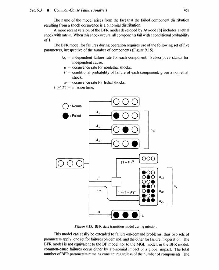
Sec. 9.3 • Common-Cause Failure Analysis 465
The name of the model arises from the fact that the failed component distributionresulting from a shock occurrence is a binomial distribution.
A more recent version of the BFR model developed by Atwood [8] includes a lethalshock with rate to. When this shock occurs, all components fail with a conditional probabilityof 1.
The BFR model for failures during operation requires use of the following set of fiveparameters, irrespective of the number of components (Figure 9.15).
A;c == independent failure rate for each component. Subscript ic stands forindependent cause.
J.l == occurrence rate for nonlethal shocks.P == conditional probability of failure of each component, given a nonlethal
shock.to == occurrence rate for lethal shocks.
t (:s T) == mission time.
o :Normal000
e :FailedA;c eooA;c oeo n;c
A;c ooe
000
J1
1 - (1 _ p)m
eoooeo n+1ooeeeaaee n+2eoeeee n+3
Figure 9.15. BFR state transition model during mission.
This model can easily be extended to failure-on-demand problems; thus two sets ofparameters apply; one set for failures on demand, and the other for failure in operation. TheBFR model is not equivalent to the BP model nor to the MGL model; in the BFR model,common-cause failures occur either by a binomial impact or a global impact. The totalnumber of BFR parameters remains constant regardless of the number of components. The

466 System Quantificationfor Dependent Events _ Chap. 9
(9.210)
BFR model treats each event as a lethal or nonlethal shock, and single failures are classifiedas independent or nonlethal. The beta-factor model, on the other hand, only describeslethal-shock common-cause events.
For a three-component system, for example, the following relations hold between BPand BFR models (t: mission time).
Arl t == Aiet + iu P( 1 - P)2jAr 2t == iu p 2( 1 - P)Ar 3t == iu p 3 + cut
The BFR model includes the beta-factor model as a special case when J-l == O.
9.3.5.2 Parameterestimation. Todevelopestimators for the parameters, additionalquantities are used.
T == run time for the system.u ; == rate of nonlethal shocks that cause at least one component failure.ni, == number of nonlethal shocks that cause i simultaneous failures.n; == L7~1 ns, = total number of nonlethal shocks that cause at least
one component failure.s == L7~1 in i, == number of component failures by nonlethal shocks.
n L == number of occurrences of lethal shocks.nic == the number of single-component failures not counting failuresdue
to lethal and nonlethal shocks (nie + n+1 == n I).
The maximum-likelihood estimators for the parameters Aie, J-l+, and ware
Aie == nie/(m T) ju ; == n.i.t Tw==nL/T
From the definition of u.; and J-l
u; == J-l[l - (I - p)m]
(9.211)
(9.212)
Thus the nonlethal shock rate J-l is calculated when parameter P is known.
J-l+u. = 1 _ (I _ P)'" (9.213)
The expected number of component failuresper nonlethal shock is mP. Furthermore,the expected number of nonlethal shocks during the total run time T is J-lT. Thus the totalnumber s of nonlethal shock component failures is estimated as
(9.214)
(9.215)s==
Substituting J-l of (9.213) into the above equation,
J.1+TmP n+mP
1 - (I - P)11l I - (1 - P)11l
Parameter P is the solution of this equation, and rate J-l is now calculatable from (9.213).
Example 16-0ne-out-of-three pump-system run failure. Consider the data inTable 9.14, which is a modified version of Table 9.11. Note that all single failures are due to in-dependent causes in.: = 45, n+l = 0); the simultaneous failure of three pumps is due to the lethal
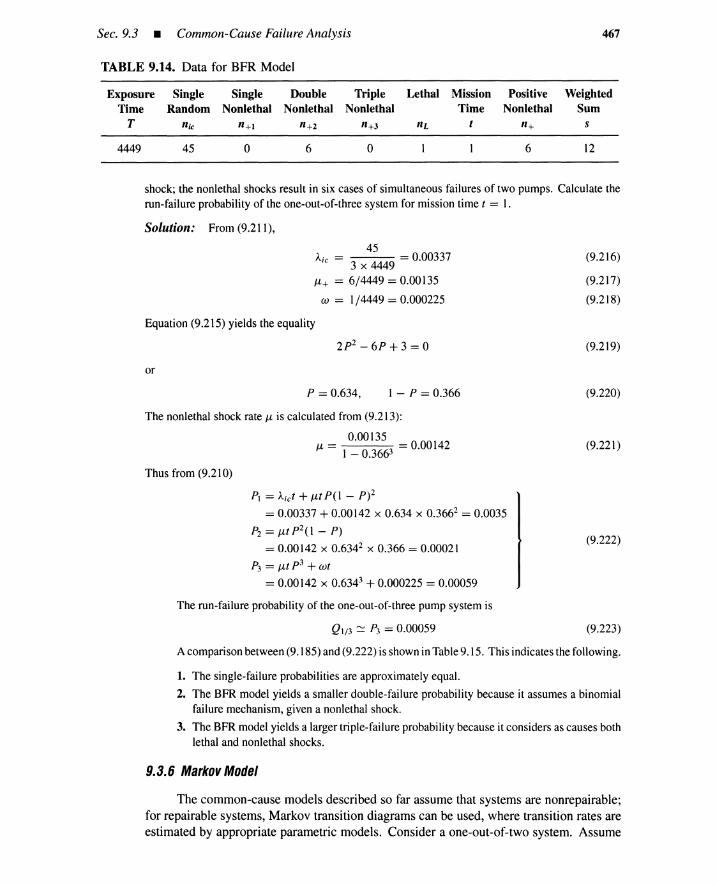
Sec. 9.3 • Common-Cause Failure Analysis 467
TABLE 9.14. Data for BFR Model
Exposure Single Single Double Triple Lethal Mission Positive WeightedTime Random Nonlethal Nonlethal Nonlethal Time Nonlethal Sum
T nic n+l n+2 n+3 nL t n+ s
4449 45 0 6 0 6 12
shock; the nonlethalshocks result in six cases of simultaneous failuresof two pumps. Calculate therun-failure probabilityof the one-out-of-three system for mission time t = 1.
Solution: From (9.211),
45Aie = 3 x 4449 = 0.00337
J-L+ = 6/4449 = 0.00135
w = 1/4449 = 0.000225
Equation(9.215) yields the equality
2p2- 6P + 3 = 0
or
(9.216)
(9.217)
(9.218)
(9.219)
P = 0.634, 1 - P = 0.366 (9.220)
The nonlethal shock rate J-L is calculatedfrom (9.213):
0.00135u. = 1 _ 0.3663 = 0.00142
Thus from (9.210)
PI = Aiet + ut P(1 - p)2
= 0.00337 + 0.00142 x 0.634 x 0.3662 = 0.0035
P2 = iu p 2(1 - P)
= 0.00142 X 0.6342 x 0.366 = 0.00021
P3 = ut p 3 + cot
= 0.00142 x 0.6343 + 0.000225 = 0.00059
The run-failureprobabilityof the one-out-of-three pump system is
QI/3 ::: P., = 0.00059
(9.221)
(9.222)
(9.223)
Acomparison between(9.185) and(9.222) is showninTable9.15. This indicatesthefollowing.
1. The single-failure probabilities are approximately equal.
2. The BFR model yields a smaller double-failure probability because it assumes a binomialfailure mechanism, givena nonlethal shock.
3. The BFRmodelyieldsa largertriple-failure probabilitybecauseit considersas causes bothlethal and nonlethal shocks.
9.3.6 Markov Model
The common-cause models described so far assume that systems are nonrepairable;for repairable systems, Markov transition diagrams can be used, where transition rates areestimated by appropriate parametric models. Consider a one-out-of-two system. Assume

468 System Quantification for Dependent Events _ Chap. 9
TABLE 9.15. BP and BFR for 1/3 PumpSystem Run Probability
BP BFR
PI 0.0034 0.0035P2 0.00045 0.00021P3 0.00022 0.00059 •
that the system is subject to a common cause C that occurs with rate Ar 2, and that eachcomponent has an independent failure rate Arl and repair rate u, Then the behavior ofthe cut set can be expressed by the Markov transition diagram of Figure 9.16, where theindicator variable 1 denotes the existence of component failure, and the variable 0 thenonexistence. A cut set fails when it falls into state (I, I). Common cause C creates themultiple-component transition from state (0, 0) to (I, I).
J1 J1
Figure 9.16. Transition diagram for 1/2system subject to commoncause.
The beta-factor model shows that rates Ar2 and Ar I can be calculated from the overallcomponent failure rate Ar and parameter fJr:
Ar2 == fJr Ar, ArI == (I - fJr) Ar (9.224)
Denote by P;j the probability of state (i, j). The following equation holds.
Poo -(2Arl + Ar2) Jl Jl 0 PooPOI Arl -(Arl + Ar2+ Jl) 0 Jl POI
(9.225)PIO Arl 0 -(Arl + Ar2+ Jl) Jl PIOPI I Ar2 Arl +Ar2 Arl + Ar2 -2Jl Pll
Let lj be the probability of the state where j components are failed: Po == Poo,PI == POI +PIO, and P2 == PI I . Equation (9.225) can be rewritten as a three-state differentialequation (Figure 9.17).
( ~o) (-(2Ar l + Ar 2)PI == 2Ar l
P2 Ar2
Jl-(Arl + Ar 2 + J-L)
Arl + Ar 2
o )(PO)2Jl PI-2Jl P2
(9.226)
The failed-state probability P2 can be calculated numerically.

Chap. 9 • Problems
Figure 9.17. Simplified common-causediagram.
REFERENCES
469
[1] Fleming, K. N., A. Mosleh, and R. K. Deremer. "A systematic procedure for theincorporation of common cause events into risk and reliability models," Nuclear En-gineering and Design, vol. 93, pp. 245-273, 1986.
[2] Dyer, D. "Unification of reliability/availability/repairability models for Markov sys-tems," IEEE Trans. on Reliability, vol. 38, no. 2, pp. 246-252, 1989.
[3] Fleming, K. N. "A reliability model for common mode failure in redundant safetysystems." In Proc. of the Sixth Annual Pittsburgh Conference on Modeling and Sim-ulation. General Atomic Report GA-AI3284, April, pp. 23-25,1975.
[4] Pickard, Lowe and Garrick, Inc. "Seabrook station probabilistic safety assessment."Prepared for Public Service Company of New Hampshire and Yankee Atomic ElectricCompany, PLG-0300, December 1983.
[5] Marshall, A. W., and I. Olkin. "A multivariate exponential distribution," J. of theAmerican Statistical Association, vol. 62, pp. 30-44, 1967.
[6] Fleming, K. N., et al. "Classification and analysis of reactor operating experienceinvolving dependent events." Pickard, Lowe and Garrick, Inc., PLG-0400, preparedfor EPRI, February 1985.
[7] Vesely, W. E. "Estimating common cause failure probabilities in reliability and riskanalyses: Marshall-Olkin specializations." In Proc. of the Int. Conf. on Nuclear Sys-tems Reliability Engineering and Risk Assessment, pp. 314-341, 1977.
[8] Steverson, J. A., and C. L. Atwood. "Common cause fault rates for valves." USNRC,NUREG/CR-2770, February 1983.
[9] USNRC. "PRA procedures guide: A guide to the performance of probabilistic risk as-sessments for nuclear power plants." USNRC, NUREG/CR-2300, 1983, Appendix B.
PROBLEMS
9.1. Let P(t) and A be an n-vector and an n x n matrix. It can be shown that the differentialequation
P(t) = AP(t)
can be solvedsequentially as
P(~) = exp(A~)P(O)
P(k~) = exp(A~)P([k - l]~)
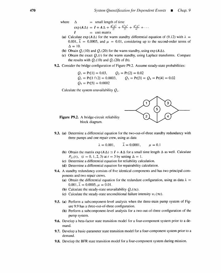
470 System Quantification for Dependent Events _ Chap. 9
where ~ = small length of timeexp(A~) = I +A~ + A2~2 + A~~~ + A4~4 + ...
2! 3! 4!
I = unit matrix(a) Calculate exp (A~) for the warm standby differential equation of (9.12) with A =
0.00 I, I = 0.0005, and Jl = 0.0 I, considering up to the second-order terms of~ = 10.
(b) Obtain Qr(IO) and Qr(20) for the warm standby, using exp (A~).
(c) Obtain the exact Qr(t) for the warm standby, using Laplace transforms. Comparethe results with Qr(IO) and Qr(20) of (b).
9.2. Consider the bridge configuration of Figure P9.2. Assume steady-state probabilities:
QI = Pr{ I} = 0.03, Q2 = Pr{2} = 0.02Qr = Pr{ I n 2} = 0.0003, Q3 = Pr{3} = Q4 = Pr{4} = 0.02Q5 = Pr{5} = 0.0002
Calculate the system unavailability Q.\..
Figure P9.2. A bridge-circuit reliabilityblock diagram.
9.3. (a) Determine a differential equation for the two-out-of-three standby redundancy withthree pumps and one repair crew, using as data
A=O.OOI, I = 0.0001, Jl = 0.1
(b) Obtain the matrix exp (A~) ~ I +A~ for a small time length ~ as well. CalculateP(i)(t), (i = 0, 1,2,3) at t = 3 by setting ~ = l.
(c) Determine a differential equation for reliability calculation.(d) Determine a differential equation for repairability calculation.
9.4. A standby redundancy consists of five identical components and has two principal com-ponents and two repair crews.(a) Obtain the differential equation for the redundant configuration, using as data A =
0.001, I = 0.0005, Jl = 0.01.(b) Calculate the steady-state unavailability Q,.(oo).(c) Calculate the steady-state unconditional failure intensity wr(oo).
9.5. (a) Perform a subcomponent-level analysis when the three-train pump system of Fig-ure 9.9 has a three-out-of-three configuration.
(b) Perform a subcomponent-level analysis for a two-out-of-three configuration of thepump system.
9.6. Develop a beta-factor state transition model for a four-component system prior to a de-mand.
9.7. Develop a basic-parameter state transition model for a four-component system prior to ademand.
9.8. Develop the BFR state transition model for a four-component system during mission.

10uman Reliability
10.1 INTRODUCTION
Humans design, manufacture, install reliable and safe systems, and function as indispensableworking elements in systems where monitoring, detection, diagnosis, control, manipula-tion, maintenance, calibration, or test activities are not automated. We can operate plantsmanually when automatic control fails.
However, to quote Alexander Pope, "to err is human." Human errors in thinking androte tasks occur, and these errors can destroy aircraft, chemical plants, and nuclear powerplants. Our behavior is both beneficial and detrimental to modem engineering systems.The reliability and safety analyst must consider the human; otherwise, the analysis is notcreditable.
It is difficult to provide a unified, quantitative description of the positive and negativeaspects of human beings in terms of reliability and safety parameters. However, a unifiedview is necessary if we are to analyze and evaluate. As a first approximation, the human isviewed as a computer system or electronic robot consisting of a main CPU, memory units,I/O devices, and peripheral CPUs. This view is, of course, too simple. Differences amonghumans, computer systems, and robots must be clarified [1].
We begin in Section 10.2 with a human-error classification scheme suitable for PRAs.Section 10.3 compares human beings with hardware systems supported by computers. Thecomparison is useful in understanding humans; we are not machines to the extent that somemachines behave like us; machines are only tools to simulate and extend human functions.Sections 10.4 and 10.5 describe how various factors influence human performance. Exam-ples of human errors are presented in Section 10.6. A general process for human-error PRAquantification is given in Section 10.7. This process is called SHARP (systematic humanaction reliability procedure [2,3].
Section 10.8 presents a quantification approach suitable to maintenance and testingprior to an accident. An event-tree-based model to quantify human-error events that ap-pear in event and fault trees is developed. This methodology is called THERP (technique
471

472 Human Reliability _ Chap. 10
for human-error rate prediction) [4-6]. Although THERP is a systematic and powerfultechnique for quantifying routine or procedure-following human tasks, it has limitations indealing with thought processes like accident diagnosis. The remaining two sections dealwith the thought process. Section 10.9 describes the HCR (human cognitive reliability)model [7, 3] to quantify nonresponseerror probabilities under time stressduring an accident.Unfortunately, the nonresponse error is not the only failure modeduring an accident; humanbehavior is unpredictable, and wrong actions that cause hazardous consequences are oftenperformed. Section 10.10deals with wrong actions.
10.2 CLASSIFYING HUMAN ERRORS FOR PRA
Event and fault trees should include human-error events taking place before and after initi-ating events. These can then be analyzed by human reliability analysts using the error typesproposed by SHARP.
10.2.1 Before anInitiating Event
This is called a pre-initiator error (see Chapter 3). There can be at least two types ofhuman errors prior to an initiating event [3]:
1. Test and Maintenance Errors: These occur under controlled conditions (e.g., noaccident, little or no time pressure) before an initiating event. A typical exampleis failure to return safety equipment to its working state after a test, thus causing alatent failure of the safety system. Most test and maintenanceactivitiesare routine,procedure-following tasks. These types of human errors must be included in faulttrees, and quantification is based on direct data, expert judgment, and/or THERP.
2. Initiating-Event Causation: An accident may be initiated by human error, par-ticularly during start-ups or shutdowns, when there is a maximum of human in-tervention. The initiating events, of course, appear as the first heading in anyevent tree, and human errors are included in the appropriate fault trees describinginitiating-eventoccurrences. This type of error can be assessed similarly to the testand maintenanceerrors; the PRA assessments are traditionally based on initiating-event frequency data such as, for example, that 40 to 50% of unnecessary nuclearpower plant trips are caused by human error,
10.2.2 During anAccident
This is a post-initiator human error containing accident-procedure errors and recov-ery errors (see Chapter 3). Wakefield [8] gives typical human response activities duringaccidents.
1. Manual backup to automatic plant response.
2. Change of normal plant safety response.
3. Recovery and repair of failed system.
4. Total shift to manual operation.
The tree shown in Figure 10.1 represents generalized action sequences taken duringan accident [3]. This is an operator action tree (OAT), as proposed by Wreathall [9]. Theevent-tree headings are arranged in the following order.
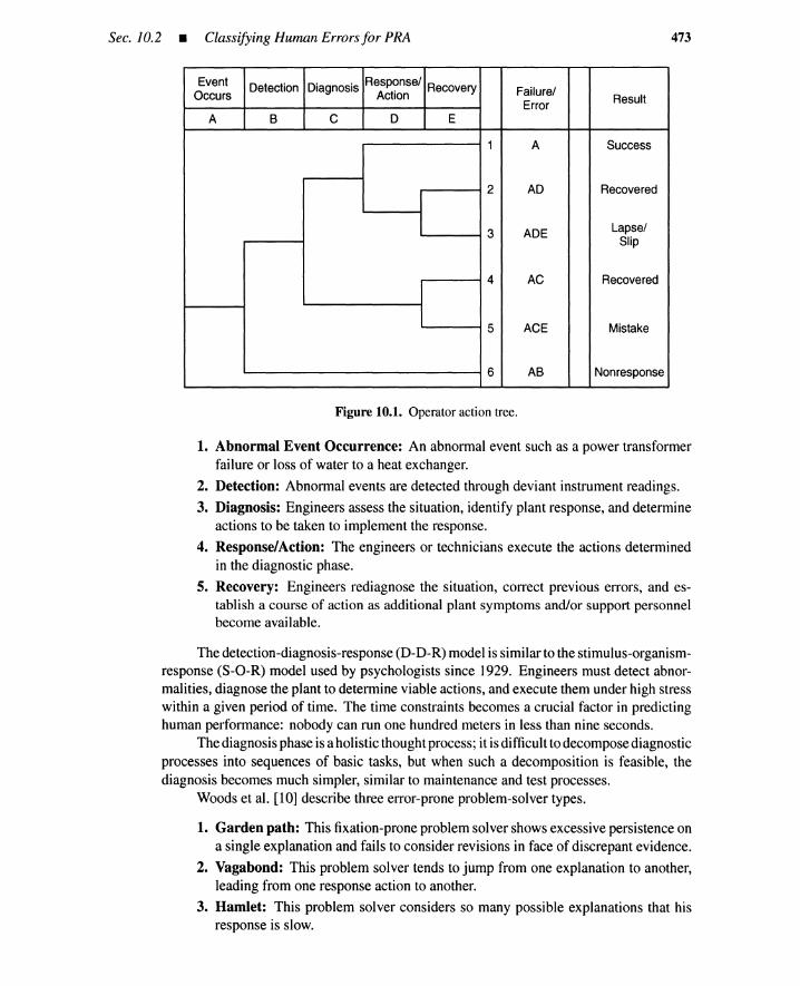
Sec. 10.2 • Classifying Human Errors for PRA
Event Detection Diagnosis Response/ RecoveryOccurs Action Failure/
ResultErrorA B C D E
1 A Success
2 AD Recovered
3 ADE Lapse/Slip
4 AC Recovered
5 ACE Mistake
6 AS Nonresponse
Figure 10.1. Operatoraction tree.
473
1. Abnormal Event Occurrence: An abnormal event such as a power transformerfailure or loss of water to a heat exchanger.
2. Detection: Abnormal events are detected through deviant instrument readings.
3. Diagnosis: Engineers assess the situation, identify plant response, and determineactions to be taken to implement the response.
4. Response/Action: The engineers or technicians execute the actions determinedin the diagnostic phase.
5. Recovery: Engineers rediagnose the situation, correct previous errors, and es-tablish a course of action as additional plant symptoms and/or support personnelbecome available.
The detection-diagnosis-response (D-D-R) model is similar to the stimulus-organism-response (S-O-R) model used by psychologists since 1929. Engineers must detect abnor-malities, diagnose the plant to determine viable actions, and execute them under high stresswithin a given period of time. The time constraints becomes a crucial factor in predictinghuman performance: nobody can run one hundred meters in less than nine seconds.
The diagnosis phase is a holistic thought process; it is difficult to decompose diagnosticprocesses into sequences of basic tasks, but when such a decomposition is feasible, thediagnosis becomes much simpler, similar to maintenance and test processes.
Woods et al. [10] describe three error-prone problem-solver types.
1. Garden path: This fixation-prone problem solver shows excessive persistence ona single explanation and fails to consider revisions in face of discrepant evidence.
2. Vagabond: This problem solver tends to jump from one explanation to another,leading from one response action to another.
3. Hamlet: This problem solver considers so many possible explanations that hisresponse is slow.
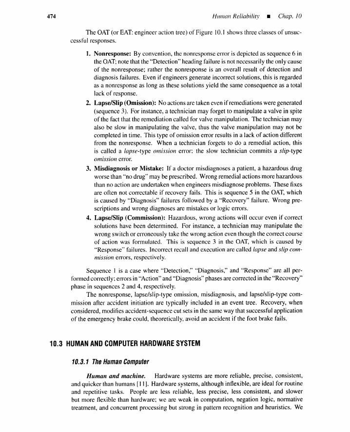
474 Human Reliability _ Chap. 10
The OAT (or EAT: engineer action tree) of Figure 10.1 shows three classes of unsuc-cessful responses.
1. Nonresponse: By convention, the nonresponse error is depicted as sequence 6 inthe OAT; note that the "Detection" heading failure is not necessarily the only causeof the nonresponse; rather the nonresponse is an overall result of detection anddiagnosis failures. Even if engineers generate incorrect solutions, this is regardedas a nonresponse as long as these solutions yield the same consequence as a totallack of response.
2. Lapse/Slip (Omission): No actions are taken even if remediations were generated(sequence 3). For instance, a technician may forget to manipulate a valve in spiteof the fact that the remediation called for valve manipulation. The technician mayalso be slow in manipulating the valve, thus the valve manipulation may not becompleted in time. This type of omission error results in a lack of action differentfrom the nonresponse. When a technician forgets to do a remedial action, thisis called a lapse-type omission error: the slow technician commits a slip-type0111issio11 error.
3. Misdiagnosis or Mistake: If a doctor misdiagnoses a patient, a hazardous drugworse than "no drug" may be prescribed. Wrong remedial actions more hazardousthan no action are undertaken when engineers misdiagnose problems. These fixesare often not correctable if recovery fails. This is sequence 5 in the OAT, whichis caused by "Diagnosis" failures followed by a "Recovery" failure. Wrong pre-scriptions and wrong diagnoses are mistakes or logic errors.
4. Lapse/Slip (Commission): Hazardous, wrong actions will occur even if correctsolutions have been determined. For instance, a technician may manipulate thewrong switch or erroneously take the wrong action even though the correct courseof action was formulated. This is sequence 3 in the OAT, which is caused by"Response" failures. Incorrect recall and execution are called lapse and slip com-111;SS;011 errors, respectively.
Sequence I is a case where "Detection," "Diagnosis," and "Response" are all per-formed correctly; errors in "Action" and "Diagnosis" phases are corrected in the "Recovery"phase in sequences 2 and 4, respectively.
The nonresponse, lapse/slip-type omission, misdiagnosis, and lapse/slip-type com-mission after accident initiation are typically included in an event tree. Recovery, whenconsidered, modifies accident-sequence cut sets in the same way that successful applicationof the emergency brake could, theoretically, avoid an accident if the foot brake fails.
10.3 HUMAN AND COMPUTER HARDWARE SYSTEM
10.3.1 The Human Computer
Human and machine. Hardware systems are more reliable, precise, consistent,and quicker than humans [II]. Hardware systems, although inflexible, are ideal for routineand repetitive tasks. People are less reliable, less precise, less consistent, and slowerbut more flexible than hardware; we are weak in computation, negation logic, normativetreatment, and concurrent processing but strong in pattern recognition and heuristics. We

Sec. 10.3 • Human and Computer Hardware System 475
are flexible in manipulation, data sensing, and data processing where the same purpose canbe accomplished by different approaches. Hardware is predictable, but human behavioris unpredictable; we can commit all types of misdiagnosis and wrong actions. Peoplefrequently lie to absolve themselves from blame. Human beings are far superior in self-correction capability than machines. Humans are purposeful; they form a solution and actaccordingly, searching for relevant information and performing necessary actions along theway. This goal-oriented behavior is good as long as the solution is correct; otherwise, thewrong solution becomes a dominant source of common-cause failures. We can anticipate.We have strong intuitive survival instincts.
Two-level computer configuration. A typical computer hardware system for con-trolling a manufacturing plant is configured in two levels; it has a main CPU and peripheralCPUs. Input devices such as pressure or temperature sensors gather data about plant states.The input CPUs at the periphery of the computer system process the raw input data and sendfiltered information to the main CPU. The main CPU processes the information and sendscommands to the output CPUs, which control the output devices. Simple or routine controlscan be performed by the 110 CPUs, which may bypass the main CPU. The peripheral CPUshave some autonomy.
Life-support ability. Figure 10.2 is a simplistic view of the human being as a com-puter system. A major difference between Figure 10.2 and the usual computer configurationis the existence of a life-support unit consisting of the "old CPU" and internal organs. Thelife-support unit is common to all animals. The old CPU is a computer that controls theinternal organs and involuntary functions such as respiration, blood circulation, hormonesecretion, and body temperature. We usually consume less energy than hardware of similarsize and ability. The old CPU senses instinctively and, in the case of a normal humanbeing, instructs it to seek pleasant sensations and avoid unpleasant ones. For example, ifa plant operator is instructed to monitor displays located far apart in a large control room,the operator tends to look at the displays from far away to minimize walk-around [4]. Thisinstinctive response prompts reading errors.
Sensing ability. The input devices in Figure 10.2 are sense organs such as eyes,ears, nose, and skin proprioceptors. Each device is not linked directly to the new CPU;each sense organ has its own CPU linked with the new CPU. This is similar to a two-levelcomputer configuration. A visual signal, for instance, is processed by its own CPU, whichdiffers from the one that processes audible signals. The multi-CPU configuration at theperiphery of sensory organs enables input devices to function concurrently; we can see andhear simultaneously.
Manipulative ability. Human output devices are motor organs such as hands, feet,mouth, and vocal chords. These motor organs are individually controlled by efferent nerveimpulses from the brain. The sophisticated output CPU servomechanism controls eachmotor organ to yield voice or body movement. An experienced operator can function as anear-optimal PID controller with a time lag of about 0.3 s. However, even an experiencedtypist commits typing errors. Computer systems stand still, but the human ambulates. Thismobility can be a source of trouble; it facilitates the type of deliberate nullification ofessential safety systems that occurred at Three Mile Island and Chernobyl.
Memorizing ability. The "new CPU" in the brain has associated with it a memoryunit of about 1012 bits. Some memory cells are devoted to long-term memory and others
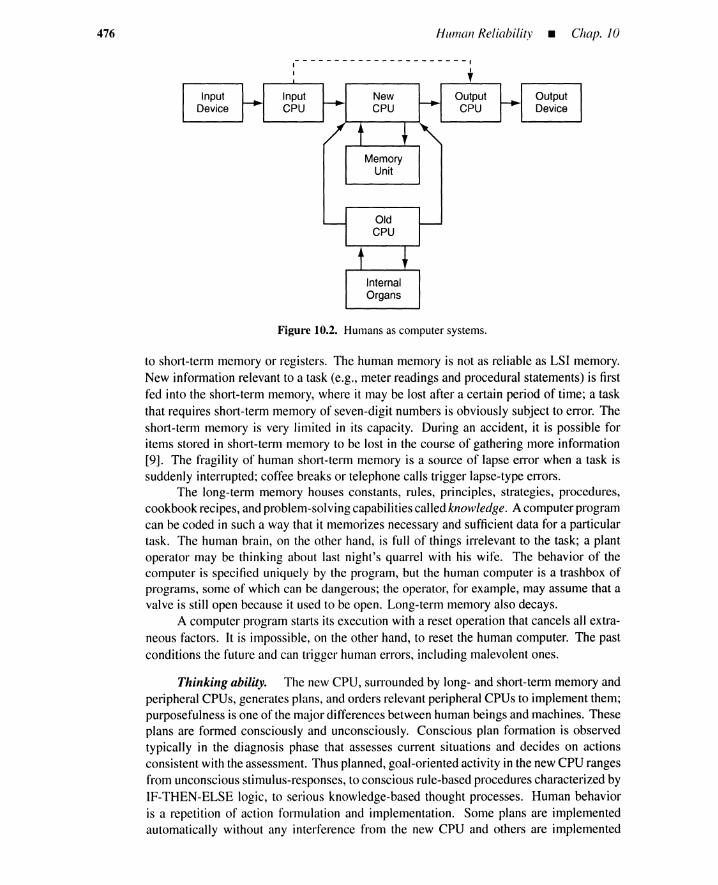
476 Human Reliability _ Chap. J0
Figure 10.2. Humans as computer systems.
to short-term memory or registers. The human memory is not as reliable as LSI memory.New information relevant to a task (e.g., meter readings and procedural statements) is firstfed into the short-term memory, where it may be lost after a certain period of time; a taskthat requires short-term memory of seven-digit numbers is obviously subject to error. Theshort-term memory is very limited in its capacity. During an accident, it is possible foritems stored in short-term memory to be lost in the course of gathering more information[9]. The fragility of human short-term memory is a source of lapse error when a task issuddenly interrupted; coffee breaks or telephone calls trigger lapse-type errors.
The long-term memory houses constants, rules, principles, strategies, procedures,cookbook recipes, and problem-solving capabilities called knowledge. A computer programcan be coded in such a way that it memorizes necessary and sufficient data for a particulartask. The human brain, on the other hand, is full of things irrelevant to the task; a plantoperator may be thinking about last night's quarrel with his wife. The behavior of thecomputer is specified uniquely by the program, but the human computer is a trashbox ofprograms, some of which can be dangerous; the operator, for example, may assume that avalve is still open because it used to be open. Long-term memory also decays.
A computer program starts its execution with a reset operation that cancels all extra-neous factors. It is impossible, on the other hand, to reset the human computer. The pastconditions the future and can trigger human errors, including malevolent ones.
Thinking ability. The new CPU, surrounded by long- and short-term memory andperipheral CPUs, generates plans, and orders relevant peripheral CPUs to implement them;purposefulness is one of the major differences between human beings and machines. Theseplans are formed consciously and unconsciously. Conscious plan formation is observedtypically in the diagnosis phase that assesses current situations and decides on actionsconsistent with the assessment. Thus planned, goal-oriented activity in the new CPU rangesfrom unconscious stimulus-responses, to conscious rule-based procedures characterized byIF-THEN-ELSE logic, to serious knowledge-based thought processes. Human behavioris a repetition of action formulation and implementation. Some plans are implementedautomatically without any interference from the new CPU and others are implemented

Sec. 10.3 • Human and Computer Hardware System 477
consciously, as by a novice golf player. Humans can cope with unexpected events. We canalso anticipate. We are very good at pattern recognition.
The processing speed of the new CPU is less than 100 bits per second-far slowerthan a computer, which typically executes several millions of instructions a second: Thehuman being can read only several words a second. The sense organs receive a huge amountof information per second. Although the raw input data are preprocessed by the peripheralinput CPUs, this amount of inflowing information is far larger than the processing speed ofthe new CPU. This slow processing speed poses difficulties, as will be described in Section10.3.2. The new CPU resolves this problem by, for instance, "scan and sample by priority,"and "like-to-like matching." The new CPU is also weak in handling negation logic; ANDor OR logic is processed more easily than NAND or NOR; this suggests that we shouldavoid negative sentences in written procedures. A normative approach such as game theoryis not to be expected.
10.3.2 Brain Bottlenecks
As stated in Section 10.3.1, the new CPU processing speed is slow and the short-termmemory capacity is small. The long-term memory capacity is huge and the sense organsreceive a tremendous amount of information from external stimuli. Because of its slowprocessing speed, the new CPU is the bottleneck in the Figure 10.2 computer configurationand is responsible for most errors, so it is quite natural that considerable attention has beenpaid to human-error rates for tasks involving the new CPU, especially for time-limiteddiagnostic thought processes during accidents.
The human computer system is an unbalanced time-sharing system consisting of aslow main computer linked to a large number of terminals. Considering the large discrep-ancy in performance, it is amazing that, historically, the human being has functioned asan indispensable element of all systems. It is also not surprising that most designers ofspace-vehicles, nuclear plants, complex weapons systems, and high-speed aircraft wouldlike to replace humans with hardware; because of improvements in hardware, human er-rors have become important contributors to accidents. Human evolution is slower thanmachine evolution. Let us now briefly discuss how the new CPU bottleneck manifestsitself.
1. Shortcut: People tend to simplify things to minimize work loads. Proceduralsteps or system elements irrelevant to the execution of current tasks are discarded.This tendency is dangerous when protection devices are nullified or safety-relatedprocedures are neglected.
2. Perseverance: When an explanation fits the current situation, there is a tendencyto believe that this explanation is the only one that is correct. Other explanationsmay well fit the situation, but these are automatically rejected.
3. Task fixation: The input information is scanned and sampled by priority, as ismemory access. The prioritization leads to task-fixation errors, which occur whenpeople become preoccupied with one particular task (usually a trivial one) to theexclusion of other tasks that are usually more important. People tend to concentrateon particular indicators and operations, while neglecting other, possibly critical,items.
4. Alternation: This occurs when an engineer constantly changes a decision whilebasic information is not changing [9]. Systematic responses become unavailable.

478 Human Reliability _ Chap. 10
5. Dependence: People tend to depend on one another. Excessive dependenceon other personnel, written procedures, automatic controllers, and indicators aresometimes harmful,
6. Naivety: Once trained, humans tend to perform tasks by rote and to bypass thenew CPU. Simple stimulus-response manipulations that yield unsafe results oc-cur. Naivety is characterized by thought processes typified by inductive logic orprobability; this logic assumes that things repeat themselves in a stationary world.Inductive logic often fails in nonstationary situations and plant emergencies.
7. Queuing and escape: This phenomenon typically occurs when the work load istoo high.
8. Gross discrimination: Details are neglected. Both scanning range and speedincrease; qualitative rather than quantitative information is collected.
9. Cheating and lying: When the human thinks it is to its advantage, it will lie andcheat. In America, over 85% of all college students admit to cheating on theirschool work.
Reason [12] lists basic error tendencies. From a diagnosis point of view, these includethe following.
1. Similarity bias: People tend to choose diagnostic explanations based on like-to-like matching.
2. Frequency bias: People tend to choose diagnostic explanations with a high fre-quency of past success.
3. Bounded rationality: People have only limited mental resources for diagnosis.
4. Imperfect rationality: People rarely make diagnoses according to optimal or nor-mative theories (e.g., logic, statistical decision theory, subjective expected utility,etc.).
5. Reluctant rationality: People perform diagnoses that minimize conscious think-ing. According to Henry Ford, the average worker wants a job in which he doesnot have to think.
6. Incomplete/incorrect knowledge: Human knowledge is only an approximationof external reality. We have only a limited number of models about the externalworld.
Human-machine systems should be designed in such a way that machines help peopleachieve their potential by giving them support where they are weakest [11,13], and viceversa. For instance, carefully designed warning systems are required to relieve humanbeings of unnecessary thought processes and guide human beings according to appropriatepriorities. A good procedure manual may present several candidate scenarios and suggestwhich one is most likely. Displays with hierarchical arrangements save scanning time anddecrease the work load. The human computer has a very unbalanced configuration and thusrequires a good operating system and peripheral engineering intelligence to mitigate newCPU bottlenecks.
10.3.3 Human Performance Variations
Determinism and indeterminism. Electronic computers, which are deterministicmachines, have internal clocks that tick several million times a second, and programs are

Sec. 10.3 • Human and Computer Hardware System 479
executed in exact accordance with the clock. Each memory cell has a fixed bit capacity andstores an exact amount of data, and the arithmetic unit always performs calculations to afixed precision. The processing speed and program execution results remain constant overmany trials, given the same initial condition and the same input data. Human computers, onthe other hand, have indeterministic, variable performance and yield different results overmany trials.
Five performance phases. The following five phases of human performance typifythe new CPU [14].
1. Unconscious phase: This occurs in deep sleep or during brain paroxysms orseizures. The new CPU intelligence stops completely.
2. Vacant phase: Excessive fatigue, monotony, drugs, or liquor can induce a vacantphase. The new CPU functions slowly.
3. Passive phase: This is observed during routine activities. The new CPU functionspassively. Display-panel monitoring during normal situations is often done in thisphase.
4. Active phase: The brain is clear and the new CPU functions actively at its bestperformance level, searching for new evidence and solutions. This phase does notlast long, and a passive phase follows shortly.
5. Panic phase: Excessive tension, fear, or work load bring on this phase. The newCPU stresses, overheats, lacks cool judgment, and loses rationality.
Visceral causes ofperformance variation. Diverse mechanisms characterize thehuman computer performance variation. We now describe one mechanism specific to thehuman being as an animal, namely, the performance variation occurs because the new CPUis controlled by the old CPU, the visceral function system. The following three controlmodes are typical [14].
1. Activity versus rest rhythm: Excessive fatigue, be it mental or physiological,is harmful. Given that fatigue occurs, the old CPU commands the new CPU torest. This phenomenon occurs typically with a one-day cycle. Figure 10.3 shows afrequency profile of traffic accidents caused by overfatigued drivers on a Japanesehighway. The horizontal axis denotes hours of the day. We observe that thenumber of accidents involving asleep-at-the-wheel drivers is a maximum in theearly morning when the one-day rhythm commands the new CPU to sleep. It isalso interesting that the TMI accident started at 4 A.M.; the operators in the controlroom were most likely in a vacant phase when they failed to correctly interpret the85 alarms set off during the first 30 s of the accident.
2. Instinct and emotion: The old CPU senses pleasant and unpleasant feelings,whether they are emotional or rational. When pleasant sensations occur, the oldCPU activates the new CPU. This is a cost/benefit mechanism related to humanmotivation. Certain types of unpleasant feelings inactivate the new CPU. Othertypes of unpleasant feelings such as excessive fear, agony, or anxiety tend tooverheat the new CPU and drive it into the panic phase.
3. Defenseof life: When the new CPU detects or predicts a situation critical to humanlife, this information is fed back to the old CPU. A life crisis is a most unpleasantsensation; the old CPU commands the new CPU to fight aggressively or run from

480
30
(J)~
Q)
> 20.t:o0)c'5.
10Q)Q)
U5
0
Human Reliability _ Chap. 10
o 6 12
Hour
18 24
Figure 10.3. Frequency profile of traffic accidents on a highway.
danger and panic ensues. The defense-of-life instinct frequently causes people todeny and/or hide dangerous situations created by their own mistakes.
Characteristics duringpanic. Typical characteristics of the human in its defense-of-life phase are summarized below [15]. These are based on investigations of the behaviorof pilots in critical situations before airplane crashes.
1. Input channels(a) Abnormal concentration: Abnormal indications and warnings are monitored
with the highest priority. Normal information is neglected.(b) Illusion: Colors and shapes are perceived incorrectly. Size and movement are
amplified.(c) Gross perception: People try to extract as much information as possible in
the time available. The speed and range of scanning increase and data inputprecision degrades.
(d) Passive perception: Excessive fatigue and stress decrease desire for moreinformation. The eyes look but do not see.
(e) Paralysis: Input channels are cut off completely.
2. Processing at the new CPU(a) Local judgment: Global judgment becomes difficult. A solution is searched
for, using only that part of the information that is easily or directly discernible.(b) Incorrect priority: Capability to select important information decreases.(c) Degraded matching: It becomes difficult to compare things with patterns
stored in memory.(d) Poor accessibility: Failures of memory access occurs. Irrelevant facts are
recalled.(e) Qualitative judgment: Quantitative judgment becomes difficult: Alljudgment
is qualitative.(f) Pessimism: The action time remaining is underestimated and thought pro-
cesses are oversimplified; important steps are neglected.(g) Proofs: Decisions are not verified.(h) Complete paralysis: Information processing at the new CPU stops completely.(i) Escape: Completely irrelevant data are processed.
Sec. 10.4 • Performance-Shaping Factors 481
3. Output channels(a) Routine response: Habitual or skilled actions are performed unconsciously.(b) Poor choice: Switches and levers are selected incorrectly.(c) Excessive manipulation: Excessive force is applied to switches, buttons,
levers, and so on. Muscle tensions and lack of feedback make smooth manip-ulations difficult. Overshooting and abrupt manipulations result.
(d) Poor coordination: It becomes difficult to coordinate manipulation of twothings.
(e) Complete irrelevance: A sequence of irrelevant manipulations occurs.(f) Escape: No manipulation is performed.
We see that most of these characteristics are extreme manifestations of bottlenecksin the new CPU together with survival responses specific to animal life.
10.4 PERFORMANCE-SHAPING FACTORS
Any factor that influences human performance is called a PSF (performance-shaping factor).The PSFs from Handbook [4] are shown in Table 10.1. These PSFs are divided into threeclasses: internal PSFs operating within the individual, external PSFs existing outside theindividual, and stressors. The external factors are divided into situational characteristics,job and task instructions, and task and equipment characteristics, while the stressors arepsychological and physiological. The internal PSFs are organismic factors and representinternal states of the individual. Psychological and physiological stress levels of an indi-vidual vary according to discrepancies between the external PSFs, such as complexity, andinternal PSFs, including previous training and experience; for instance, experienced driversdo not mind driving in traffic, whereas novices do.
10.4.1 Internal PSFs
Internal PSFs are divided into three types: hardware, psychological, and cognitive.
Hardware factors. These fall into four categories: physiological, physical, patho-logical, and pharmaceutical.
1. Physiological factors: Humans are organisms whose performance depends on, forexample, physiological factors caused by fatigue, insufficient sleep, hangovers,hunger, 24-hour rhythms, and hypoxia. These factors are also related to envi-ronmental conditions such as low atmospheric pressure, work load, temperature,humidity, lighting, noise, and vibration.
2. Physical factors: These refer to the basic capabilities of the body as typified bysize, force, strength, flexibility, eyesight, hearing, and quickness.
3. Pathological factors: These include diseases such as cardiac infarction and AIDs;mental diseases such as schizophrenia, epilepsy, and chronic alcoholism; and self-induced trauma.
4. Pharmaceutical factors: These refer to aberrant behavior caused by sleepingtablets, tranquilizers, antihistamines, and an extremely large variety of illegaldrugs.
Psychologicalfactors. These include fear, impatience, overachievement, overcon-fidence, motivation (or lack of it), anxiety, overdependence, introversion, or other emotional
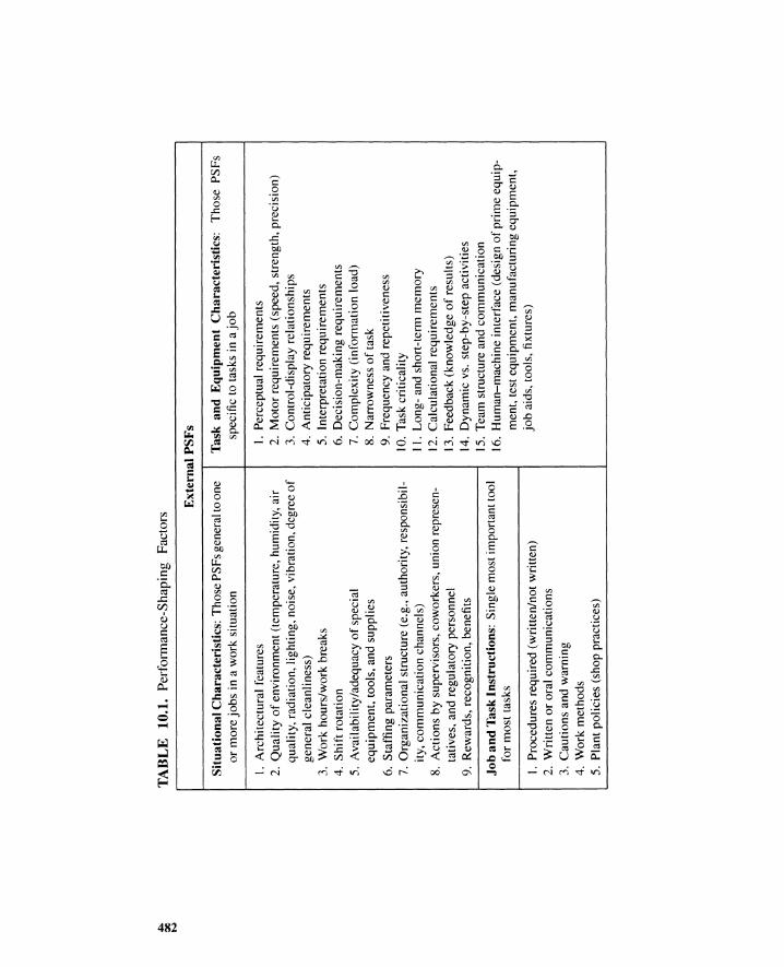
~ QO~
TA
BL
E10
.1.
Per
form
ance
-Sha
ping
Fact
ors
Ext
erna
lP
SF
s
Sit
uati
onal
Cha
ract
eris
tics
:T
hose
PSFs
gene
ral
toon
eor
mor
ejo
bs
ina
wor
ksi
tuat
ion
l.A
rchi
tect
ural
feat
ures
2.Q
ual
ity
of
envi
ronm
ent
(tem
pera
ture
,hu
mid
ity,
air
qual
ity,
radi
atio
n,li
ghti
ng,
nois
e,vi
brat
ion,
degr
eeo
fge
ner a
lcl
eanl
ines
s)3.
Wor
kho
urs/
wor
kbr
eaks
4.Sh
ift
rota
tion
5.A
vail
abil
ity/
adeq
uacy
of
spec
ial
equ
ipm
ent,
tool
s,an
dsu
ppli
es
6.S
taff
ing
para
met
ers
7.O
rgan
izat
iona
lst
ruct
ure
(e.g
.,au
thor
ity,
resp
onsi
bil-
ity,
com
mun
icat
ion
chan
nels
)8.
Act
ions
bysu
perv
isor
s,co
wor
kers
,un
ion
repr
esen
-ta
tive
s,an
dre
gula
tory
pers
onne
l9.
Rew
ards
,re
cogn
itio
n,be
nefi
ts
Job
and
Tas
kIn
stru
ctio
ns:
Sin
gle
mos
tim
port
antt
ool
for
mos
tta
sks
1.P
roce
dure
sre
quir
ed(w
ritt
en/n
otw
ritt
en)
2.W
ritt
enor
oral
com
mun
icat
ions
3.C
auti
on
san
dw
arni
ng4.
Wor
km
etho
ds5.
Pla
ntpo
lici
es(s
hop
prac
tice
s)
Tas
kan
dE
quip
men
tC
hara
cter
isti
cs:
Tho
seP
SF
ssp
ecif
icto
task
sin
ajo
b
1.P
erce
ptua
lre
quir
emen
ts2.
Mot
orre
quir
emen
ts(s
peed
,st
reng
th,
prec
isio
n)3.
Con
trol
-dis
play
rela
tion
ship
s4.
Ant
icip
ator
yr e
quir
emen
ts5.
Inte
rpre
tati
onr e
quir
emen
ts6.
Dec
isio
n-m
akin
gr e
quir
emen
ts7.
Com
plex
ity
(inf
orm
atio
nlo
ad)
8.N
arro
wne
sso
fta
sk9.
Fre
quen
cyan
dre
peti
tive
ness
10.
Tas
kcr
itic
alit
y11
.L
ong-
and
shor
t-te
rmm
emo
ry12
.C
alcu
lati
onal
requ
irem
ents
13.
Fee
dbac
k(k
now
ledg
eo
fre
sult
s)14
.D
ynam
icvs
.st
ep-b
y-st
epac
tivi
ties
15.
Tea
mst
ruct
ure
and
com
mun
icat
ion
16.
Hum
an-m
achi
nein
terf
ace
(des
ign
ofpr
ime
equi
p-m
ent,
test
equi
pmen
t,m
anuf
actu
ring
equi
pmen
t,jo
bai
ds,
tool
s,fi
xtur
es)

TA
BL
E10
.1.
Con
tinu
ed
Str
esso
rPS
Fs
Psy
chol
ogic
alS
tres
sors
:PS
Fsth
atdi
rect
lyaf
fect
men
-ta
lst
ress
1.S
udde
nnes
so
fon
set
2.D
urat
ion
ofst
ress
3.T
ask
spee
d4.
Tas
klo
ad5.
Hig
hje
opar
dyri
sk6.
Thr
eats
( of
failu
re,
loss
ofjo
b)7.
Mon
oton
ous/
degr
adin
g/m
eani
ngle
ssw
ork
8.L
ong,
unev
entf
ulvi
gila
nce
peri
ods
9.C
onfl
icts
of
mot
ives
abou
t jo
bpe
rfor
man
ce10
.R
einf
orce
men
tab
sent
orne
gativ
eII
.S
enso
ryde
priv
atio
n12
.D
istr
acti
ons
(noi
se,
glar
e,m
ovem
ent,
flic
ker,
colo
r)13
.In
cons
iste
ntcu
eing
Phy
sica
lS
tres
sors
:P
SF
sth
atdi
rect
lyaf
fect
phys
ical
stre
ss
I.D
urat
ion
of
stre
ss2.
Fat
igue
3.Pa
inor
disc
omfo
rt4.
Hun
ger
orth
irst
5.T
empe
ratu
reex
trem
es6.
Rad
iati
on7.
G-f
orce
extr
emes
8.A
tmos
pher
icpr
essu
reex
trem
es9.
Oxy
gen
insu
ffic
ienc
y10
.V
ibra
tion
II.
Mov
emen
tco
nstr
icti
on12
.L
ack
of
phys
ical
exer
cise
13.
Dis
rupt
ion
of
Cir
cadi
anrh
ythm
Inte
rnal
PS
Fs
Org
anis
mic
Fac
tors
:
~ QO~
I.P
revi
ous
trai
ning
expe
rien
ce2.
Sta
teo
fcu
rren
tpr
acti
ceor
skill
3.P
erso
nali
tyan
din
tell
igen
ceva
riab
les
4.M
otiv
atio
nan
dat
titu
des
5.E
mot
iona
lst
ate
6.S
tres
s(m
enta
lor
bodi
lyte
nsio
n)
7.K
now
ledg
eo
fre
quir
edpe
rfor
man
cest
anda
rds
8.Se
xdi
ffer
ence
s9.
Phy
sica
lco
ndit
ion
10.
Att
itud
esba
sed
onin
flue
nce
offa
mily
and
othe
rou
tsid
epe
rson
sor
agen
cies
II.
Gro
upid
enti
fica
tion
s

484 Human Reliability _ Chap. J0
instabilities. Overachievement, for instance, may cause a maintenance person to disconnecta protective device while making an unscheduled inspection of a machine, thus creating ahazard. Non-optimal workplace stress levels lead to abnormal psychological states. Psy-chological and physiological factors interact.
Cognitivefactors. These are classified into skill-based abilities, rule-based abilities,and knowledge-based abilities.
1. Skill-based factors: These are concerned with levels of skill required to movehands or feet while performing routine activities. Practice improves these skills;thus routine activities are usually performed quickly and precisely. These skills areanalogous to hard-wired software. Reflex-based mobility is especially importantin crisis situations where time is a critical element. Reflex-based motor skills,however, are sometimes harmful because reflex actions can occur when they arenot desired. The same can be said of routine thought processes.
2. Rule-based factors: These refer to the performance of sequential or branchedtasks according to rules in manuals, checklists, or oral instructions. These rulesare typified by IF-THEN-ELSE logic. Rule-based activities tend to become skill-based after many years of practice.
3. Knowledge-based factors: These refer to a level of knowledge relating to plantschematics, principles of operation, cause-consequence relations, and other in-telligence. Knowledge utilized in problem solving is called cues [13]. The cuesinclude interpreted, filtered, and selective stimuli or data; a series ofrules; schemas;templates; lessons learned; and/or knowledge chunks for making a judgment ordecision.
The physiological, physical, pathological, pharmaceutical, and psychological factorsare called the six P's by Kuroda [15], who also considers psychosocial states. Althoughpathological or pharmaceutical factors are important, they could be neglected if we assumehuman quality control, or healthy people. This assumption, unfortunately, is frequentlyunjustified. An airplane crash occurred in Japan in 1981 when a pilot suffering fromschizophrenia "maliciously" retrofired the jet engines just before landing. We could alsoneglect physical factors, provided that the human performing the task is basically capable ofdoing it. Then three factors remain: physiological, psychological, and cognitive. The firsttwo factors are relatively short-term in nature, the third is long-term. In other words, thephysiological and psychological factors may change from time to time, resulting in varyinglevels of physiological and psychological stresses.
In the following section we will discuss how the human computer in Figure 10.2behaves when linked with external systems.
10.4.2 External PSFs
When linked with external systems, the human computer performance level variesdynamically with the characteristics of the external system and the individual person'sinternal states. Some PSFs apply to computer systems; others are specific to humans. Thesituational characteristics define background factors common to all human tasks; thesecharacteristics form the environment under which tasks are performed.
The tasks consist of elementary activities such as selection, reading, manipulation,and diagnosis. The performance-shaping factors specific to each unit activity are called taskand equipment characteristics in Table 10.1. The instructions associated with a sequence
Sec. 10.4 • Performance-Shaping Factors 485
of unit activities go under the title of job and task instructions. The stressors are factors ofpsychological or physiological origin that decrease or increase stress levels.
Situational characteristics
1. Architectural factors: This refers to workplace characteristics, and includes suchparameters as space, distance, layout, size, and number.
2. Quality of environment: Temperature, humidity, air quality, noise, vibration,cleanliness, and radiation are factors that influence hardware performance. Thesame is true for humans. Psychological stresses, however, are specific to people;technicians try to finish jobs quickly under poor environments such as noxiousodors or high temperatures; this is specific to humans.
3. Work hours/work breaks: Hardware must be periodically maintained, and somust the human.
4. Shift rotation: Unfortunately, apres moi le deluge attitudes are not uncommon.
5. Availability/adequacy of special equipment, tools, and supplies: Printers can-not print without paper or ribbon. Humans also require equipment, tools, andsupplies. For better or worse, humans can do jobs without proper tools. A majoraccident at the Browns Ferry nuclear power plant was caused by a maintenanceman who used a candle flame to check for air leaks.
6. Staffing parameters: In multicomputer systems it is important to allocate tasksoptimally. The same is true of humans. Job dissatisfaction is a frequent cause ofpsychological stress and can engender uncooperative activities, and even sabotage.
7. Organizational structure: This includes authority, responsibility, and commu-nication channels. These are typical of multicomputer systems in a hierarchicalconfiguration, but psychological effects are specific to human beings.
8. Actions by supervisors, coworkers, union representatives, and regulatory per-sonnel: The regulatory infrastructure of the workplace is very important (seeChapter 12). The human computer is subject to many influences. Occasionally,he or she is told to strike, or the government may declare the person's workplaceto be unsafe.
9. Rewards, recognition, benefits: These are obviously specific to human beings.
Task and equipment characteristics. As described earlier, these characteristicsrefer to factors concerned with the degrees of difficulty of performing an activity.
1. Perceptual requirements: Visual indicators are more common than audiblesignals. Human eyesight, however, is limited; it may be difficult to read fourdigits from a strip-chart recorder. Some displays are easier to read than others.
2. Motor requirements (speed, strength, precision): Each engineering manipu-lator or actuator has limited speed, strength, or precision. The same is true forhuman motor organs.
3. Control-display relationships: Displays must be suggestive of control actions.If a display guides an operator toward an incorrect control mechanism, the prob-ability of human error increases, especially under highly stressful situations; thestress factor is a psychological effect specific to human beings.
4. Anticipatory requirements: If an activity requires an operator to anticipatewhich display or control becomes important in the future, while performing a
486 Human Reliability _ Chap. J0
current function, humanerror increases. Humancomputersare essentially inone-channel configurations and are not good at performing two or more proceduresconcurrently. The computer can execute several procedures concurrently in atime-sharing mode because of its high processing speeds and reliable memory.
5. Interpretation requirement: An activity requiring interpretation of informa-tion is more difficult than a routine activity because the interpretation itself is anadditional, error-prone activity. Response times become longer and human errorincreases. The same is true for computer software. People interpret informationin different ways, and this is a contributing factor to the high frequency of er-rors during shift changes; similar phenomena are observed when an operation istransformed from one computer system to another. The shift-change accidentsoccur because people lie. The last group does not want to tell the new group thatanything is wrong: "Blame it on the next guy."
6. Decision-making requirement: A decision-making function makes an activitymore attractive and increases volition. Absence of decision-making functionsleads to boredom. These are psychological effects not generic to computers.Correct information must be provided if the decision maker is to select appro-priate alternatives. This requirement applies also to an electronic computer.Decision-makingfunctions must beconsistent with the capability of each individ-ual; similarly,a computer system requires software capable of making decisions.Decision-making increases stress levels.
7. Complexity (information load): The complexity of an activity is related to theamount of informationto be processedand the complexity of the problem-solvingalgorithm. Error probability increases with complexity; this is common to boththe human being and the computer.
8. Narrowness of task: General-purpose software is more difficult to design andmore error-prone than special-purpose software. The latter, however, lacks flex-ibility.
9. Frequency and repetitiveness: Repetition increases both human and computersoftware reliability. Human beings, however, tend to be bored with repetitions.Rarely performed activities are error-prone. This corresponds to the bum-inphase forcomputer software. Just as an electronic system requires simulated testsfor validation, human beings must be periodically trained for rarely performedactivities. Fire and lifeboat drills are a necessity.
10. Task criticality: In a computer program with interrupt routines, critical tasksare executed with highest priority. Humans also have this capability, providedthat activities are suitably prioritized. Psychological stress levels increase withthe criticality of an activity; stress levels may be optimal, too high, or too low.
11. Long- and short-term memory: Human short-term memory is very fragilecompared to electronic memory. Reliable secondary storage to assist humans isrequired.
12. Calculational requirement: Human beings are extremely low-reliabilitycalcu-lators compared to computers.
13. Feedback (knowledge of results): Suitable feedback improvesperformance forboth human beings and computers; it is well known that closed-loop control ismore reliable than open-loop control. Time lags degrade feedback-controllerperformance; for people, a time lag of more than several seconds is critical for

Sec. 10.4 • Performance-Shaping Factors 487
certain types of process control. Feedback is also related to motivation, and thisis specific to human beings.
14. Continuity (discrete versus continuous): Continuity refers to correlation ofvariables in space and time. Dynamic multivariable problems are more difficultto solve than static, single-variable ones. The former are typified by the following.(a) Some variables are not directly observable and must be estimated.(b) Variables are correlated.(c) The controlled process has a large time lag.(d) Humans tend to rely on short-term memory because various display indica-
tors should be interpreted collectively.(e) Each unit process is complicated and difficult to visualize.
15. Team structure and communication: In some cases, an activity performed byone team member is verified by another. This resembles a mutual check provisionin a two-computer system. Social aspects, such as collapse of infrastructure andconspiracy, are specific to human beings.
16. Human-machine interface: This refers to all interface factors between thehuman and machine. System designers usually pay considerable attention tointerfaces between computers and machines. Similar efforts should be paid to thehuman-machine interfaces. The factors to be considered include the following.(a) Design of display and control: functional modularization, layout, shape,
size, slope, distance, number, number of digits, and color.(b) Display labeling: symbol, letter, color, place, standardization, consistency,
visibility, access, and content.(c) Indication of plant state: clear and consistent correspondence between indi-
cators and plant states, and consistent color coding.(d) Amount of information displayed: necessary and sufficient warning signals,
prioritized displays, hierarchical indications, and graphical display.(e) Labeling and status indication of hardware: indication of hardware operating
modes, visibility and clarity of labels.(I) Protection provisions: fail-safe, foolproof, lock mechanisms, and warning
devices.
Job and task instructions. In a computer, where menu-driven software is used, cer-tain types of input data instruct the general-purpose software to run in a certain way. Thesedata are indexed, paged, standardized, and modularized, especially when processing speedis a critical factor. Humans represent general-purpose software in the extreme. Instructionsin the form of written or oral procedures, communications, cautions, and warnings shouldbe correct and consistent with mental bottlenecks. For instance, a mixture of safety-relatedinstructions and property damage descriptions on the same page of an emergency manualincrease mental overload; column formats are more readable than narrative formats.
Stressors. The physiological and psychological stressors in Table 10.1 are specificto human beings. The TMI accident had a "suddenness of onset" factor because when ithappened, few people believed it actually did.
10.4.3 Types ofMental Processes
Three types of mental processing are considered in the HeR model [7,3]. Reference[3] defines the three types below.

488 Human Reliability _ Chap. 10
1. Skill-based behavior: This behavior is characterized by a very close couplingbetween sensory input and response action. Skill-based behavior does not dependdirectly on the complexity of the task, but rather on the level of training andthe degree of practice in performing the task. A highly trained worker performsskill-based tasks swiftly or even mechanically with a minimum of errors.
2. Rule-based behavior: Actions are governed by a set of rules or associations thatare known and followed. A major difference between rule-based and skill-basedbehaviors stems from the degree of practice. If the rules are not well practiced,the human being has to recall consciously or check each rule to be followed.Under these conditions the human response is less timely and more prone to errorsbecause additional cognitive processes must be called upon. The potential forerror results from problems with memory, the lack of willingness to check eachstep in a procedure, or failure to perform each and every step in the procedure inthe proper sequence.
3. Knowledge-based behavior: Suppose that symptoms are ambiguous or complex,the plant state is complicated by multiple failures or unusual events, or instru-ments give only indirect readings of the plant state. Then the engineer has to relyon personal knowledge, and behavior is determined by more complex cognitiveprocesses. Rasmussen calls this knowledge based behavior [16,17]. Human per-formance in this type of behavior depends on knowledge of the plant and abilityto use that knowledge. This type of behavior is expected to be more prone to errorand to require more time.
Figure 10.4shows a logic tree to determine the expected mental processing type. It isassumed that, for the routine task, the operator clearly understands the corresponding plantstates. For the routine task, we see
1. If the routine task is so simple that itdoes not requirea procedure, then the behavioris skill-based (sequence I).
2. Even if the operator requires a procedure for the routine task, the behavior isskill-based when the operator is practiced in the procedure (sequence 2).
3. If the operator is not well practiced in the routine task procedure, then behavior isrule-based (sequence 3).
4. If a routine task procedure is unavailable, then behavior is rule-based becausebuilt-in rules must be used (sequence 4).
Consider next the nonroutine task. If the operator does not have a clear understandingof the corresponding plant state, then behavior is knowledge-based (sequence 9) becausethe plant must first be diagnosed. The following sequences consider the case when there isan understanding of the plant state, equivalent to a successful plant diagnosis.
1. If no procedures are available, then the behavior is knowledge-based (sequence 8)because the procedure itself must be invented.
2. If the procedure is not understood, then the behavior is knowledge-based(sequence7) because it must first be understood.
3. If the procedure is well understood, behavior is rule-based (sequence 6) when theoperator is not well practiced in the procedure.
4. With understanding and practice, behavior becomes skill-based.
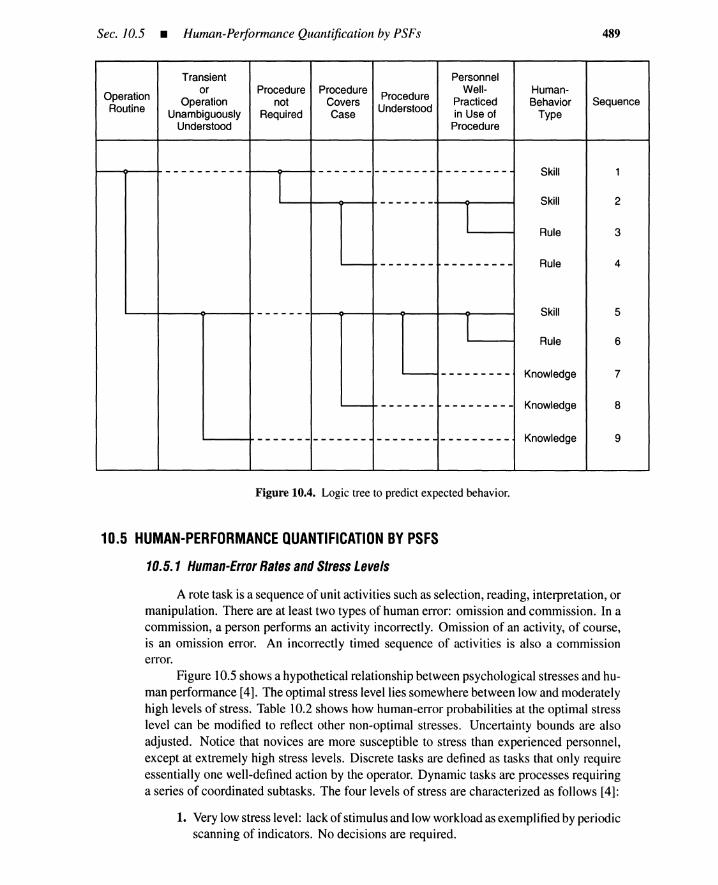
Sec. 10.5 • Human-Performance Quantification by PSFs 489
Transient Personnel
Operationor Procedure Procedure
ProcedureWell- Human-
Operation not Covers Practiced Behavior SequenceRoutine Unambiguously Required Case
Understood in Use of TypeUnderstood Procedure
--_ ... _----- ------- -------- 1--------- Skill 1
I ------- Skill 2
1 Rule 3
1..0-- ------- --------- Rule 4
------- Skill 5
1 Rule 6
---- --------- Knowledge 7
----- ------- --------- Knowledge 8
------- ------- -------- --------- Knowledge 9
Figure 10.4. Logic tree to predict expected behavior.
10.5 HUMAN-PERFORMANCE QUANTIFICATION BY PSFS
10.5.1 Human-Error Rates and Stress Levels
A rote task is a sequence of unit activities such as selection, reading, interpretation, ormanipulation. There are at least two types of human error: omission and commission. In acommission, a person performs an activity incorrectly. Omission of an activity, of course,is an omission error. An incorrectly timed sequence of activities is also a commissionerror.
Figure 10.5 shows a hypothetical relationship between psychological stresses and hu-man performance [4]. The optimal stress level lies somewhere between low and moderatelyhigh levels of stress. Table 10.2 shows how human-error probabilities at the optimal stresslevel can be modified to reflect other non-optimal stresses. Uncertainty bounds are alsoadjusted. Notice that novices are more susceptible to stress than experienced personnel,except at extremely high stress levels. Discrete tasks are defined as tasks that only requireessentially one well-defined action by the operator. Dynamic tasks are processes requiringa series of coordinated subtasks. The four levels of stress are characterized as follows [4]:
1. Very low stress level: lack of stimulus and low workload as exemplified by periodicscanning of indicators. No decisions are required.
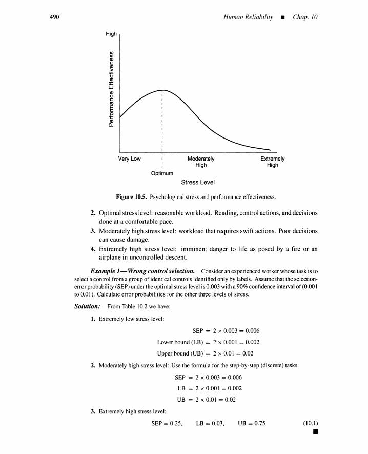
490 Human Reliability _ Chap. 10
High
enenQ)cQ)>UQ):t:UJQ)occoE'-o't:Q)
a..
Very Low
Optimum
ModeratelyHigh
Stress Level
ExtremelyHigh
Figure 10.5. Psychological stress and performanceeffectiveness.
2. Optimal stress level: reasonable workload. Reading,control actions, anddecisionsdone at a comfortable pace.
3. Moderately high stress level: workload that requires swift actions. Poor decisionscan cause damage.
4. Extremely high stress level: imminent danger to life as posed by a fire or anairplane in uncontrolled descent.
Example 1-Wrong control selection. Consideran experiencedworkerwhose task is toselect a control from a group of identicalcontrols identifiedonly by labels. Assume that the selection-error probability(SEP) under the optimal stress levelis 0.003 witha 90% confidenceintervalof (0.00Ito 0.0 I). Calculate error probabilities for the other three levelsof stress.
Solution: From Table 10.2 we have:
1. Extremely low stress level:
SEP = 2 x 0.003 = 0.006
Lower bound (LB) = 2 x 0.001 = 0.002
Upper bound (UB) = 2 x 0.0 I = 0.02
2. Moderately high stress level: Use the formula for the step-by-step (discrete) tasks.
SEP = 2 x 0.003 = 0.006
LB = 2 x 0.001 = 0.002
UB = 2 x 0.0 I = 0.02
3. Extremely high stress level:
SEP = 0.25, LB = 0.03, UB = 0.75 (10.1)
•
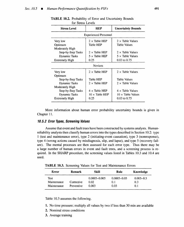
Sec. 10.5 • Human-Performance Quantification by PSFs
TABLE 10.2. Probability of Error and Uncertainty Boundsfor Stress Levels
Stress Level I HEP Uncertainty Bounds
Experienced Personnel
Very low 2 x Table HEP 2 x Table ValuesOptimum Table HEP Table ValuesModerately High
Step-by-Step Tasks 2 x Table HEP 2 x Table ValuesDynamic Tasks 5 x Table HEP 5 x Table Values
Extremely High 0.25 0.03 to 0.75
Novices
Very low 2 x Table HEP 2 x Table ValuesOptimum
Step-by-Step Tasks Table HEP Table ValuesDynamic Tasks 2 x Table HEP 2 x Table Values
Moderately HighStep-by-Step Tasks 4 x Table HEP 4 x Table ValuesDynamic Tasks lOx Table HEP lOx Table Values
Extremely High 0.25 0.03 to 0.75
491
More information about human error probability uncertainty bounds is given inChapter 11.
10.5.2 Error Types, Screening Values
Assume that event and fault trees have been constructed by systems analysts. Human-reliability analysts then classify human errors into the types described in Section 10.2: type1 (test and maintenance error), type 2 (initiating-event causation), type 3 (nonresponse),type 4 (wrong actions caused by misdiagnosis, slip, and lapse), and type 5 (recovery fail-ure). The mental processes are then assessed for each error type. Thus there may bea large number of human errors in event and fault trees, and a screening process is re-quired. In the SHARP procedure, the screening values listed in Tables 10.3 and 10.4 areused.
TABLE 10.3. Screening Values for Test and Maintenance Errors
Error Remark Skill Rule Knowledge
Test 0.0005-0.005 0.0005-0.05 0.005-0.5Maintenance Corrective 0.02 0.1 0.3Maintenance Preventive 0.003 0.03 0.1
Table 10.3 assumes the following.
1. No time pressure; multiply all values by two if less than 30 min are available
2. Nominal stress conditions
3. Average training

492 Human Reliability • Chap. 10
TABLE 10.4. Screening Values for Nonresponse and WrongActions
Error Time Skill Rule Knowledge
Nonresponse Short 0.003 0.05 1.0Nonresponse Long 0.0005 0.005 0.1Wrong action IS min 0.001 0.03 0.3Wrongaction 5 min 0.1 1.0 1.0
4. If a systematic tagging/logging procedure is in place, reduce values by 10 to 30(except for knowledge-based actions)
The following conditions are assumed for Table 10.4.
1. Human-error rates not in a database
2. Long time means longer than 1 hr
3. Short time means from 5 min to I hr
4. Screening values may be conservative by factors of 100 to 1000
For recovery errors, a screening-error probability of 1.0 is assumed; for initiating-event causation, values in abnormal event databases are assumed.
10.5.3 Response Time
A nominal median response time T1/ 2 is defined as the time corresponding to aprobability of 0.5 that a required task has been successfully carried out under nominal con-ditions [3]. This time can be found from analyses of simulator data or from interviews withplant operating crews. In the HeR (human cognitive reliability) model [7,3], representa-tive PSFs are defined as in Table 10.5 and their relations to the actual response time areformulated.
The actual median response time T1/ 2 is calculated from the nominal median responsetime T 1/ 2 by
(10.2)
Example 2-Detection ofautomatic-shutdown failure. Considerthe taskof detectingthat a failure of an automatic plant-shutdown system has occurred. The nominal median responsetime is T1/2 = 10s. Assume average operator (K1 = 0.00) under potential emergency(K2 = 0.28)with good operator/plant interface (K) = 0.00). The actual median response time T1/ 2 is estimatedto be
T1/2 = (l + 0.00)(1 + 0.28)(1 + 0.00)(10) = 12.8s (10.3)
Thus the potential emergency has lengthened the median response time by 2.8 s. Given the actualresponse time and a time limit, a nonresponse error probability can be estimated using a three-parameter Weibull reliabilitycurve, as described in Section 10.9. •
10.5.4 Integration 01 PSFs byExperts
The SLIM (success likelihood index methodology) [18] integrates various PSFs rel-evant to a task into a single number called a success likelihood index (SLI). The microcom-puter implementation is called MAUD (multiattribute utility decomposition). For a given

Sec. 10.5 • Human-Performance Quantification by PSFs
TABLE 10.5. Definition of Typical PSFs
493
PSFs CoefT. Criteria
OperatorExperience K1
1 Expert -0.22 Trainedwith more than fiveyears experience2 Average 0.00 Trained with more than six monthsexperience3 Novice 0.44 Trained with less than six monthsexperience
Stress Level K2
1 Graveemergency 0.44 High stress situation,emergency withoperatorfeel-ing threatened
2 High workload 0.28 High stress situation,part-waythroughpotentialemergency accidentwith high workloador equivalent
3 Optimalcondition(normal) 0.00 Optimal situation,crew carrying out small loadadjustments
4 Vigilance problem(low stress) 0.28 Problemwith vigilance, unexpected transientwithno precursors
Operator/Plant Interface K3
1 Excellent -0.22 Advanced operator aids are available to help in ac-cident situation
2 Good 0.00 Displayshuman-engineered with informationintegration
3 Fair 0.44 Displays human-engineered, but without informa-tion integration
4 Poor 0.78 Displaysare available, but not human-engineered5 Extremelypoor 0.92 Displaysare not directly visible to operator
SLI, the human-error probability (HEP) for a task is estimated by the formula
log(HEP) == a x SLI + b, or HEP == 10axSLI+b (10.4)
where a and b are constants determined from two or more tasks for which HEPs are known;if no data are available, they must be estimated by experts.
Consider, for instance, the PSFs: process diagnosis (0.25), stress level (0.16), timepressure (0.21), consequences (0.10), complexity (0.24), and teamwork (0.04) [19]. Thenumber in the parentheses denotes the normalized importance (weight Wi) of a particularPSF for the task under consideration, as determined by experts.
The expert must select rating R, from 0 to 1 for PSF i, Each PSF rating has an idealvalue of 1 at which human performance is judged to be optimal. These ratings are based ondiagnosis required, stress level, time pressure, consequences, complexity, and teamwork.The SLI is calculated by the following formula.
SLI == L WiRi (10.5)
Example3-SLIMquantification. Considerthe weightsand ratingvaluesinTable 10.6.The weightshave already normalized, that is, L Wi = 1. The SLI is calculatedas

494 Human Reliability _ Chap. 10
TABLE 10.6. Normalized Weights and PSFRatings for a Task
PSF Normalized Weight Rating
Process Diagnosis 0.25 0.40Stress Level 0.16 0.43Time Pressure 0.21 1.00Consequences 0.10 0.33Complexity 0.24 0.00Teamwork 0.04 1.00
SLI = (0.25)(0.40) + (0.16)(0.43) + (0.21)( 1.00) + (0.10)(0.33) + (0.24)(0.00)+(0.04)(1.00) = 0.45
10.5.5 Recovery Actions
(10.6)
•Some PSFs are important when quantifying recovery from failure. These include [8]:
1. Skill- or rule-based actions backed up by arrival of technical advisors
2. Knowledge-basedactions backedupbyarrivalof offsiteemergencyresponse teams
3. New plant measurements or samples that prompt reassessments and diagnoses'
4. Human/machine interface
10.6 EXAMPLES OF HUMAN ERROR
In this section we present typical documented examples of human errors [20-29].
10.6. 1 Errors in Thought Processes
The accidents in this section are due to wrong solutions or faulty diagnoses, notlapse-Islip-typeerrors.
Example 4-Chemical reactor explosion. After lighting the pilot flame, the operatoropened an air damper to permit 70% of maximum airflow to the burner. The air damper failed toopen because it was locked, and the flame went out due to the shortage of air. The operator purgedthe air out of the reactor, and ignited the fuel again, and incomplete combustion with excess fuel inthe reactor resulted. In the meantime, a coworker found that the air damper was locked, and releasedthe lock. An explosive mixture of fuel and air formed and the reactor exploded.
The coworker's error was in thinking that unlatching the damper would resolve the systemfault-a manifestation of frequency bias; removal of cause will frequently ensure a system's returnto the normal state; an exceptional case is where the cause leaves irreversibleeffects on the system;in this example, excess fuel concentration in the reactor was an irreversible effect. The unlatchingmanipulation is an example of a wrong action due to a faulty solution. •
Example 5-Electric shock. A worker used a defective voltage meter to verify that a440-volt line was not carrying current prior to the start of his repair. The fact that the meter wasdefective was not discoveredat the time, because he entered and repaired a switchboard box withoutreceiving a shock-because of an electric power failure. Some time later he entered the box again.

Sec. 10.6 • Examples ofHuman Error 495
He checked the voltageas before. By this time, however, the power failure had been repaired,and hewas electrocuted.
The first successful entrance made him think that he had checked the voltage correctly. Itwas difficult for him to believe that the voltage measurement was incorrect and that an accidentalpower failure allowed him to enter the switchboardbox without receiving a shock-a manifestationof frequency bias. •
Example 6-lnadvertent switch closure. An electrical device needed repair, so thepower supply was cut off. The repair took a long time and a shift change occurred. The foremanof the new shift ordered a worker to cut off the power supply to the device. However, the formershift had already opened the switch, so the workeractuallyclosed it. He told the foreman that he hadopened the switch, and the worker who started the repair was electrocuted.
It wasquitenaturalfor the workerto assumethat the switchwasclosedbecausetheforemanhadorderedhimto openit-frequency bias. Fewpeopleare skepticalenoughtodoubta naturalscenario-perseverance. This example also shows the importance of oral instructions, a performance-shapingfactor in Table 10.1. •
The following example shows human error caused by a predilection to take short-cuts.
Example 7-Warning buzzer. A buzzer that soundswhenevera red signal is encounteredis located in the cab of a train. Traffic is heavy during commuter hours; the buzzer sounds almostcontinuously, so a motormanchose to run the train with the buzzerturnedoff becausehe wasannoyedby the almost-continuous sound. One day he committed a rear-endcollision. •
Human errors caused by excessive dependence on other personnel or hardware devicesare demonstrated by the following three examples.
Example 8-Excessive dependence on automatic devices. A veteran pilot aborteda landing because an indicator light showed that the front landing gear was stuck. He climbed toan altitude of 2000 ft, switched from manual navigation to autopilot, and inspected the indicator.The autopilot failed inadvertently and minutes later the airplane crashed. None of the crew hadbeen monitoring the altimeter because they had confidence in the autopilot-this is a task-fixationerro~ •
Example 9-Excessive dependence on protective devices. A veteran motorman incharge of yard operations for bullet trains failed to notice that the on-switches of the main andemergencybrakesof a trainwerereversedon the traincontrolpanel. The yard operationwasrelativelyeasy-goingand less stressful thandrivinga bullet train. The ex-motorman,in addition,had instinctivereliance on the "triplicate" braking system and neglected to follow basic procedural steps demandedof a professional. Neither the main nor the emergencybrakes functioned, and the train ran away. Thisexamplealso relates to performance-shaping factors such as "cautions and warnings" in Job andTaskInstructionsand "monotonous work" in Psychological Stresses in Table 10.1. •
Example 10-Excessive dependence on supervisor. Figure 10.6 is a chemical plantthat generates product by reaction of liquids X and Y. A runaway reaction occurs if feed rate Ybecomes larger than X. In case of failure of the feed pump for liquid X, feed Y is automaticallycutoff, and a buffer tank supplies enough X to stabilize the reaction.
After a scheduledsix-month maintenance, an operator inadvertentlyleft valve2 in the X-feedclosed (commissionerror); this valve should have been open. Prior to start-up of the plant, operatorB inspectedthe lines but failed to notice that valve2 was closed (firstomissionerror), and returned tothe control room. OperatorB and supervisorA startedfeeding X and Y. A deficiency of X developedbecause bypass valve 4 was also closed. The buffer tank, however, functioned properly and startedto supply liquid X to the reactor. The operator stopped the start-up because a liquid-level indicatorshoweda decrease in the buffer tank level.
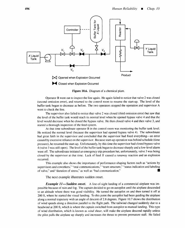
496 HUl11an Reliability _ Chap. 10
X LiquidTank
[><] Opened when Explosion Occurred
~ Closed when Explosion Occurred
ot3coQ)
a:
Product
Y LiquidTank
Figure 10.6. Diagram of a chemical plant.
Operator B went out to inspect the line again. He again failed to notice that valve2 was closed(second omission error), and returned to the control room to resume the start-up. The level of thebuffer tank began to decrease as before. The two operators stopped the operation and supervisor Awent to check the line.
The supervisor also failed to notice that valve 2 was closed (third omission error) but saw thatthe level of the buffer tank would reach its normal level when he opened bypass valve 4 and that thelevel would decrease when he closed the bypass valve. He then closed valve4 and then valve 3, andstarted a thorough inspection of the feed system.
At that time subordinate operator B in the control room was monitoring the buffer tank level.He noticed the normal level (because the supervisor had opened bypass valve 4). The subordinatehad great faith in the supervisor and concluded that the supervisor had fixed everything-an errorcaused by excessiverelianceon the supervisor. Because start-upoperation was behind schedule (timepressure), he resumed the start-up. Unfortunately, by this time the supervisorhad closed bypass valve4 (valve3 was still open). The levelof the buffer tank began to decrease sharply and a low-level alarmwent off. The subordinate initiatedan emergency trip procedure but, unfortunately, valve3 was beingclosed by the supervisor at that time. Lack of feed X caused a runaway reaction and an explosionoccurred.
This example also shows the importance of performance-shapingfactors such as "actions bysupervisorsand coworkers,""oral communications,""team structure,""status indication and labelingof valve,"and "duration of stress," as well as "bad communication." •
The next example illustrates sudden onset.
Example l l-s-Sudden onset. A line-of-sight landing of a commercial airplane was im-possible because of rain and fog. The captain decided to go on autopilot until the airplane descendedto an altitude where there was good visibility. He turned the autopilot on and then turned it off at200 ft, where he started the visual landing. To this point the autopilot had been guiding the airplanealong a normal trajectory with an angle of descent of 2.8 degrees. Figure 10.7shows the distributionof wind speeds along a direction parallel to the flight path. The tailwind changed suddenly due to aheadwind at 200 ft, which is where the captain switched from autopilot to manual landing. This typeof wind distribution, which is known as wind shear, will make the airplane descend rapidly unlessthe pilot pulls the airplane up sharply and increases the thrust to prevent premature stall. He failed
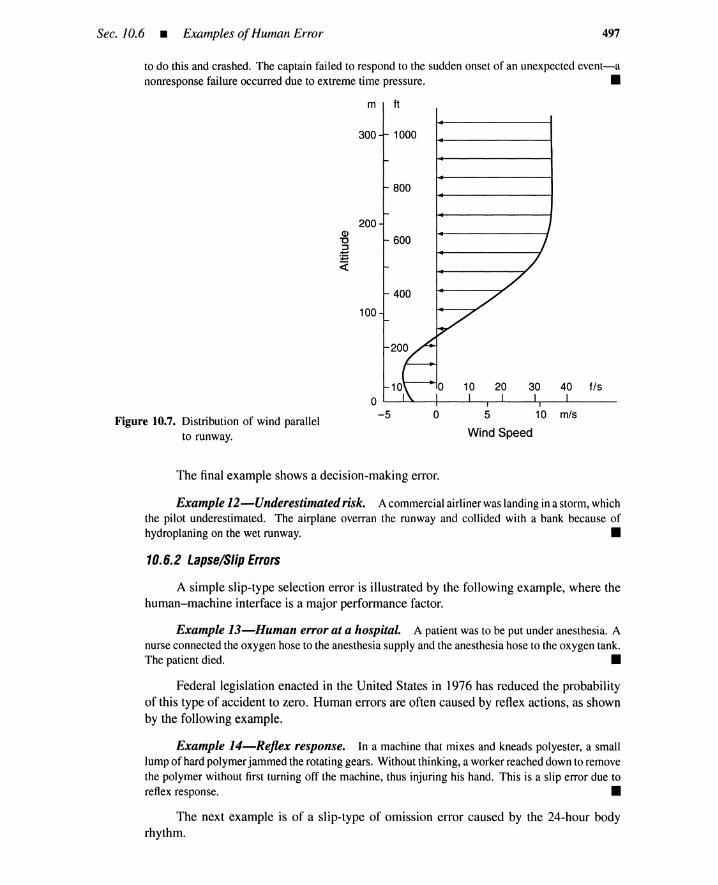
Sec. 10.6 • Examples ofHuman Error 497
to do this and crashed. The captain failed to respond to the sudden onset of an unexpected event-anonresponse failure occurreddue to extreme time pressure. •
m ft
300 1000
f/s
5 10 mls
Wind Speed
oo "'----'--l----+----"'---r-...L..----L..r----L.---
-5
800
200Q)
600"0.a+=«
400
100
Figure 10.7. Distribution of wind parallelto runway.
The final example shows a decision-making error.
Example 12-Underestimatedrisk. Acommercial airlinerwaslandingina storm,whichthe pilot underestimated. The airplane overran the runway and collided with a bank because ofhydroplaning on the wet runway. •
10.6.2 Lapse/Slip Errors
A simple slip-type selection error is illustrated by the following example, where thehuman-machine interface is a major performance factor.
Example 13-Human error at a hospital. A patient was to be put under anesthesia. Anurseconnectedthe oxygenhose to the anesthesiasupplyand the anesthesiahose to the oxygentank.The patientdied. •
Federal legislation enacted in the United States in 1976 has reduced the probabilityof this type of accident to zero. Human errors are often caused by reflex actions, as shownby the following example.
Example 14-Reflex response. In a machine that mixes and kneads polyester, a smalllumpof hardpolymerjammed the rotatinggears. Withoutthinking,a workerreacheddownto removethe polymer without first turning off the machine, thus injuring his hand. This is a slip error due toreflexresponse. •
The next example is of a slip-type of omission error caused by the 24-hour bodyrhythm.
498 HUI11an Reliability _ Chap. 10
Example IS-Driving asleep. A motorman driving a train fell asleep very late at night,failed to notice a red signal, and the train crashed. •
Human beings are especiaIJy error-prone when a normal sequence of activities isinterrupted or disturbed. There are a variety of ways of interrupting a normal sequence, asshown by Examples 16 to 20.
Example 16-1nterrupted activity. A temporary ladder was attached to a tank by twohooks. When the ladder was no longer needed, the supervisor ordered a worker to cut off the hooksand remove the ladder. The supervisor left the site, which is an interruption. The workman cut offthe hooks and left for lunch, but did not remove the ladder, which still leaned against the tank wall.The supervisor returned to the site, climbed up the ladder,and fell. A lapse-typeof commission erroroccurred due to an interruption. •
Example 17-Leaving the scene for another task. A worker started fillinga tank withLNG. He left the site to inspect some other devices and forgot about the liquified natural gas (LNG)tank. The tank was about to overflow when another worker shut off the feed. A lapse-type omissionerror occurred. •
Example 18-A distraction. An operator was asked to open circuit breaker A. As heapproached the switch box, he happened to notice that breaker B, which was adjacent to A, wasdirty. He cleaned breaker B and then opened it in place of breaker A; a slip-type commission erroroccurred. •
Example 19-Counting extra breakers. A device in circuit 2 of a four-circuit systemfailed, and a worker was ordered to open circuit breaker 2. He went to a switch box, where breakersI, 2, 3, and 4 were located in a row. The breakers were numbered right to left, but he ignored thenumbersand counted left to right. He opened breaker3 instead of breaker 2 and damaged the system.A slip was induced by the unnecessary task of counting the breakers. •
Example 20-A telephone call. An airport controller received a telephone call whilecontrolling a complicated traffic pattern. He asked another controller to take over. A near missoccurred because the substitute operator was inexperienced. •
10.7 SHARP: GENERAL FRAMEWORK
Human errors are diverse and no single model can deal with every possible aspect of humanbehaviors. SHARP provides a frameworkcommon to aIJ human-reliabilityanalysis modelsand suggests which model is best suited for a particular type of human error (for example,see Table 10.7); it also clarifies cooperative roles of systems and human-reliability analystsin performing a PRA.
SHARP consists of seven steps [3].
1. Definition: Toensure that aIJ humanerrors are adequatelyconsidered and includedin event and fault trees.
2. Screening: To identify the significant human interactions. Screening values inSection 10.5.2are chosen; consequences of human errors are considered.
3. Breakdown: To clarify various attributes of human errors. These attributes in-clude mental processes, available time, response time, stress level,and other PSFs.
4. Representation: To select and apply techniques for modeling human errors.These models include THERP, HeR, SLIM-MAUD, and confusion matrix.

Sec. 10.8 • THERP: Routine and Procedure-Following Errors
TABLE 10.7. Error Types and Quantification Methods
499
Error Type Quantification Method
Before InitiatingEvent
Test and maintenance error I THERP
For InitiatingEvent
Initiating-event causation ExperienceExpertjudgment, FT
During Accident
NonresponseWrong actionsSlip and lapseRecovery failure
HCRConfusionmatrixTHERP, SLIM-MAUDTHERP, SLIM-MAUD, HCR
5. Impact Assessment: To explore the consequences of human errors in event andfault trees.
6. Quantification: To quantify human-error probabilities, to determine sensitivities,and to establish uncertainty ranges.
7. Documentation: To include all necessary information for the assessment to betraceable, understandable, and reproducible.
In the following sections, we describe the THERP model for routine and rule-basedtasks typified by testing and maintenance before an accident, the HeR model for dealingwith nonresponse errors under time stress, and the confusion matrix model [8] for wrongactions during an accident.
10.8 THERP: ROUTINE AND PROCEDURE-FOLLOWING ERRORS
10.8.1 Introduction
In this section we describe THERP. This technique, which was first developed andpublicized by Swain, Rook, and coworkers at the Sandia Laboratory in 1962 for weapons-assembly tasks, was later used in the WASH-1400 study, and since then it has been improvedto the point where it is regarded as the most powerful and systematic methodology for thequantification of human reliability for routine and procedure-following test and maintenanceactivities. THERP is relatively weak in analyzing time-stressed thought processes such asdiagnosis during an accident, because a step-by-step analysis is frequently infeasible. Thissection is based primarily on papers by Swain, Guttmann, and Bell and the PRA ProceduresGuide [4-6].
Human errors, defined as deviations from assigned tasks, often appear as basic eventsin fault trees. A THERP analysis begins by decomposing human tasks into a sequenceof unit activities. Possible deviations are postulated for each unit activity. An event tree,called an HRA (human-reliability analysis) event tree to distinguish it from ordinary eventtrees, is then used to visualize the sequence of unit activities.
The HRA event tree is a collection of chronological scenarios associated with humantasks. Each limb of the event tree represents either a normal execution of a unit activity or

500 Human Reliability _ Chap. 10
an omission or commission error related to the activity. An intermediate hardware-failurestatus caused by a human error can be represented as a limb of an HRA tree. The humanerror appearing as a basic event in a fault tree or an ordinary event tree is defined by asubset of terminal nodes of the HRA event tree. The occurrence probability of the basicevent is calculated after probabilities are assigned to the event tree limbs. Limb-probabilityestimates must reflect performance-shaping factors specific to the plant, personnel, andboundary conditions. Events described by limbs can be statistically dependent.
Before presenting a more detailed description of THERP, we first construct an illus-trative event tree.
Example 21-HRA event tree for a calibration task. Assume that a technician isassigned the task of calibrating setpoints of three comparators that use OR logic to detect abnormalpressure [4]. The basicevent in the fault tree is that OR detection logic fails due to a calibration error.The failed-dangerous (FO) failure occurs when all three comparators are miscalibrated.
The worker must first assemble the test equipment. If he sets up the equipment incorrectly, thethree comparators are likely to be miscalibrated. The calibration task consists of four unit activities:
1. Set up test equipment
2. Calibrate comparator I
3. Calibrate comparator 2
4. Calibrate comparator 3
Figure 10.8 shows the HRA event tree. Weobserve the following conventions.
1. A capital letter represents unit-activity failure or its probability. The corresponding lower-case letter represents unit-activity success or probability.
2. The same convention applies to Greek letters, which represent nonhuman events such ashardware-failure states caused by preceding human errors. In Figure 10.8 the hardwarestates are small test-equipment-setuperror and large setup error.
3. The letters 5 and F are exceptions to the above rule in that they represent, respectively,human-task success and failure. Success in this example is that at least one comparator iscalibrated correctly; failure is the simultaneous miscalibrationof three comparators.
4. The two-limb branch represents unit-activity success and failure; each left limb expressessuccess and each right limb, failure. For hardware states, limbs are arranged from left toright in ascending order of severity of failure.
5. Limbs with zero or negligibly small probability of occurrence are removed from the eventtree. The event tree can thus be truncated and simplified.
As shown in Figure 10.8, the technician fails to correctly set up the test equipment withprobability 0.01. If she succeeds in the setup, she will correctly calibrate at least one comparator.Assume that miscalibration of each of the three comparators occurs independently with probability0.0 I; then simultaneous miscalibration occurs with probability (0.0 1)3 = 10- 6, which is negligiblysmall. The success limb a = 0.99 can therefore be truncated by success node 51,which implies thatone or more comparators are calibrated correctly.
Setup error A results in a small or a large test-equipment error with equal probability, 0.5for each. We assume that the technician sets up comparator I without noticing a small setup error.This is shown by the unit-failure probability B = 1.0. While calibrating the second comparator,however, she would probably notice the small setup error because it would seem strange that the twocomparators happen to require identical adjustment simultaneously. Probability c = 0.9 is assignedto the successful discovery of a small setup error. Success node 52 implies the same event as 51. Ifthe technician neglects the small setup error during the first two calibrations, a third calibration error

Sec. 10.8 • THERP: Routine and Procedure-Following Errors
D'= 1.0
F1 F2
A = failure to set up equipment
a = small test-equipment-setup error f3 = large test-equipment-setup errorB = small setup error/failure to detect B' = large setup error/failure to detect
first calibration error first calibration errorC =small setup error/failure to detect C' =large setup error/failure to detect
second calibration error second calibration errorD = small setup error/failure to detect D'=large setup error/failure to detect
third calibration error third calibration error
Figure 10.8. Probability tree diagram for hypothetical calibration.
501
is almost certain. This is shown by unit probability D = 1.0. Failure node F1 implies sequentialmiscalibration of three comparators.
A large test-equipment-setup error would probably be noticed during the first calibration be-cause it would seem strange that the first comparator required such a large adjustment. This is indicatedby success probability b' = 0.9 of finding the setup error. Success node S3results because the techni-cian would almost surely correct the setup error and calibrate at least one comparator correctly. Evenif the large setup error at the first calibration is neglected, it would almost surely be noticed during thesecond calibration, thus yielding success node S4 with probability c' = 0.99. The technician wouldassuredly fail to find the setup error at the third calibration if the error was neglected during the firstand second calibrations. This is evidenced by unit-failure probability D' = 1.0. Failure node F2 alsoimplies sequential miscalibration (simultaneous failure) of the three comparators.
The probability of a success or failure node can be calculated by multiplying the appropriateprobabilities along the path to the node. *
Pr{Sd = 0.99
Pr{S2} = (0.01)(0.5)(1.0)(0.9) = 0.0045
Pr{S3} = (0.01)(0.5)(0.9) = 0.0045
Pr{S4} = (0.01)(0.5)(0.1)(0.99) = 0.000495
Pr{F1} = (0.01) (0.5) (1.0) (0.1) (1.0) = 0.0005
Pr{F2} = (0.01) (0.5) (0. 1)(0.01 )(1.0) = 0.000005
Because the basic event in question is simultaneous miscalibration of three comparators, prob-ability Pr{F} of occurrence of the basic event is the sum of failure-node probabilities:
*Nonsignificant numbers are carried simply for identification purposes.

502 Human Reliability _ Chap. 10
Pr{F} = Pr{Fd + Pr{F2 }
= 0.0005 + 0.000005 = 0.000505
Probability Pr{S} of non-occurrence of the basic event is simply the complement of Pr{F}:
Pr{S} = Pr{Sd + Pr{S2} + Pr{S3} + Pr{S4}
= 0.99 + 0.0045 + 0.0045 + 0.0000495
= 0.999495 = 1 - Pr{F}
•10.8.2 General THERP Procedure
Steps in a human reliability analysis are depicted in Figure 10.9.
Plant Visit
2
3
4
5
6
7
8
9
10
11
Figure 10.9. Overview of a human- 12
reliability analysis.
ReviewInformation withFault-Tree Analysts
Talk-Through
Task Analysis
DevelopHRA EventTrees
Assign Human-ErrorProbabilities
Estimate the RelativeEffectsof Performance-
ShapingFactors
Assess Dependence
Determine SuccessandFailure Probabilities
Determine the Effectsof RecoveryFactors
Performa SensitivityAnalysis, if Warranted
Supply Information toFault-Tree Analysts
Steps 1 to 3: Plant visit to talk-through. The first three procedural steps shouldextract the following intelligence.
Sec. 10.8 • THERP: Routine and Procedure-Following Errors 503
1. Human-error-related events in the fault or event trees
2. Human tasks related to the event
3. Boundary conditions under which the tasks are performed. These include controlroom aspects, general plant layout, administrative system, time requirements, per-sonnel assignments, skill requirements, alerting cues, and recovery factors froman error after it occurs.
Step 4: Task analysis. The fourth step, task analysis, clarifies each human taskand decomposes it into a sequence of unit activities. For each unit activity, the followingaspects must be clarified.
1. The piece of equipment in question
2. Human action required
3. Potential human errors
4. Location of controls, displays, and so on.
If different tasks or activities are performed by different personnel, staffing parametersmust be identified during the task analysis.
Step 5: Developing BRA event trees. The fifth step, HRA-event-tree development,is essentially a dichotomous classification. The size of the event tree is large if many unitactivities are involved; however, its size can be reduced if the event tree is truncated, usingthe following simplifications.
1. Combining dependent events: The occurrence of an event sometimes specifiesa sequence of events. For instance, omission failure to close the first valve usuallyleads to omission failures for the remaining valves if the valves are perceived as agroup.
2. Neglecting small probabilities: If the occurrence probability in a limb of theevent tree is negligibly small, that limb and all successors can be removed fromthe tree.
3. Failure or success node: If a path in an event tree is identified as a success or afailure node of the task being analyzed, further development of the event tree fromthat node is not required.
4. Neglecting recovery factors: If one notices an error (commission or omission)after performing a unit activity and resumes the process, such a resumption con-ceptually constitutes a loop in the event tree and increases its size and complexity.Recovery factors such as cues given by annunciator displays facilitate resumptionof normalcy. It is often better, however, to postpone consideration of recovery fac-tors until after total system success and failure probabilities have been determined[6]. Estimated failure probabilities for a given sequence in an HRA event tree maybe so low, without considering the effects of recovery factors, that the sequencewill not be a dominant failure mode. In this case recovery can be dropped fromfurther consideration. As a matter of fact, "neglecting recovery factors" is analo-gous to "neglecting small probabilities": a rule that helps guide human-reliabilityanalyses toward dominant failure modes.
Step 6: Assigning human-error probabilities. The sixth step in Figure 10.9 is theassignment of estimated Handbook [4] or database probabilities to event-tree failure limbs.The data estimates are usually based on the following limiting assumptions [6].

504 HU111an Reliability _ Chap. 10
1. The plant is operating under normal conditions. There is no emergency or otherstate that produces abnormal operator stress.
2. The operator need not wear protective clothing. If protective clothing is necessary,we must assume that the operator will attempt to complete the task quickly becauseof the poor working environment. This increases human-error probability.
3. A level of administrative control roughly equal to industry-wide averages.
4. The tasks are performed by licensed, qualified plant personnel.
5. The working environment is adequate to optimal.
A reliability analyst should be familiar with the organization of the HEPs (human-error probabilities) in Chapter 20 of Swain and Guttmann's Handbook ofHuman ReliabilityAnalysis [4]. The description that most closely approximates the situation under considera-tion should be identified, and if there are discrepancies between the scenario in the Handbookand the one under consideration, the HEP should be modified to reflect actual performanceconditions. Usually, this is done during assessment of the performance-shaping factors(Le., Step 7 in Figure 10.9). Tables Al 0.6 to Al 0.13 in the Appendix list some of the HEPsin the Handbook. These are the BHEPs (basic human-error probabilities) used in the nextstep.
Step 7: Evaluating PSFs. Some of the PSFs affect the whole task, whereas othersaffect only certain types of errors. Table 10.2 indicates how BHEPs are modified by thestress level, a typical PSF.
Step 8: Assessing dependence. THERP considers five types of dependence: com-plete dependence (CD), high-level dependence (HD), moderate-level dependence (MD),low-level dependence (LD), and zero dependence (ZD), that is, independence.
Consider the labeled part of the event tree in Figure 10.10; unit activity B followsactivity A. Assume that preceding activity A fails, and let BHEP denote unconditionalfailure probability of activity B (i.e., failure probability when activity B occurs alone). Theconditional failure probability given failure of A is obtained by the following equations,which reflect five levels of dependence.
1. CD:
B == 1.0
Unit activity B always fails upon failure of activity A.
, , , , , ,
(10.7)
Figure 10.10. Event tree to illustrate de-pendency.
B
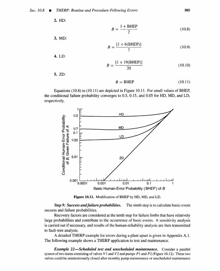
Sec. 10.8 • THERP: Routine and Procedure-Following Errors
2. HD:
1 + BHEPB==----
2
3. MD:
B == _[I_+_6_(B_H_E_P_)]7
4. LD:
B == _[I_+_I_9(_BH_E_P_)]20
5. ZD:
B == BHEP
505
(10.8)
(10.9)
(10.10)
(10.11)
Equations (10.8) to (10.11) are depicted in Figure 10.11. For small values of BHEP,the conditional failure probability converges to 0.5, 0.15, and 0.05 for HD, MD, and LD,respectively.
~1/2
:.aca.gq:
1/7'- "t-o..o 0.1'- Q)o '-'- ::J'- - 1/20w·-l cac LLcacE Q)::l.~I(!)
0.01(ij ..ceQo"t--..::;0:ac0o
0.001 '------a---'--~............._~--'--~~"'--__.......___"__'__L..........."'_--'--.......___..............1....0!001..0
0.0001 0.001 0.01 0.1
Basic Human-Error Probability (BHEP) of B
Figure 10.11. Modificationof BHEP by HD, MD, and LD.
Step 9: Success andfailure probabilities. The ninth step is to calculate basic-eventsuccess and failure probabilities.
Recovery factors are considered at the tenth step for failure limbs that have relativelylarge probabilities and contribute to the occurrence of basic events. A sensitivity analysisis carried out if necessary, and results of the human-reliability analysis are then transmittedto fault-tree analysts.
A detailed THERP example for errors during a plant upset is given in Appendix A.l.The following example shows a THERP application to test and maintenance.
Example 22-Scheduled test and unscheduled maintenance. Consider a parallelsystemof two trainsconsisting of valves V 1and V2 and pumps P I and P2 (Figure 10.12). These twovalvescould be unintentionallyclosed after monthly pump maintenance or unscheduled maintenance
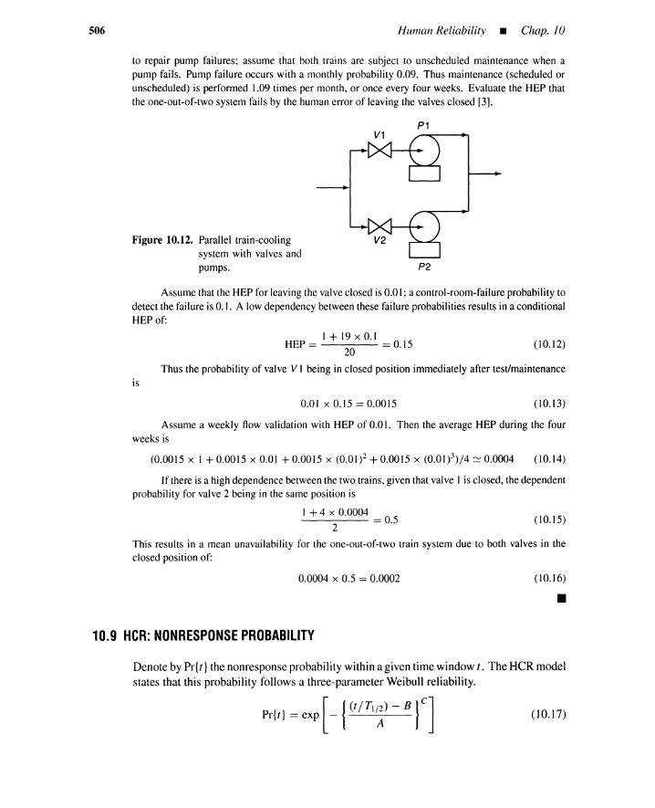
506 HU111an Reliability _ Chap. 10
to repair pump failures; assume that both trains are subject to unscheduled maintenance when apump fails. Pump failure occurs with a monthly probability 0.09. Thus maintenance (scheduled orunscheduled) is performed 1.09 times per month, or once every four weeks. Evaluate the HEP thatthe one-out-of-twosystem fails by the human error of leaving the valvesclosed [3].
P1
Figure 10.12. Parallel train-coolingsystem with valves andpumps. P2
Assume that the HEP for leaving the valveclosed is 0.0 I; a control-room-failureprobability todetect the failure is 0.1. A lowdependency between these failure probabilitiesresults in a conditionalHEP of:
1+ 19 x 0.1HEP = 20 = 0.15 (10.12)
Thus the probability of valve V I being in closed position immediately after test/maintenanceis
0.01 x 0.15 = 0.0015 (10.13)
Assume a weekly flow validation with HEP of 0.0 I. Then the average HEP during the fourweeks is
(0.0015 x I + 0.0015 x 0.0 I + 0.0015 x (0.0 1)2+ 0.0015 x (0.0 I )3) /4 :: 0.0004 (10.14)
If there is a high dependence between the two trains,given that valve I is closed, the dependentprobability for valve 2 being in the same position is
1+4 x 0.00042 = 0.5 (10.15)
This results in a mean unavailability for the one-out-of-two train system due to both valves in theclosed position of:
0.0004 x 0.5 = 0.0002 (10.16)
•10.9 HeR: NONRESPONSE PROBABILITY
Denote by Pr{ t} the nonresponse probability withina given time window t. The HeR modelstates that this probability follows a three-parameter Weibull reliability.
[ {(t I T1/2) - B } C]
Pr{t} == exp -A
(10.17)
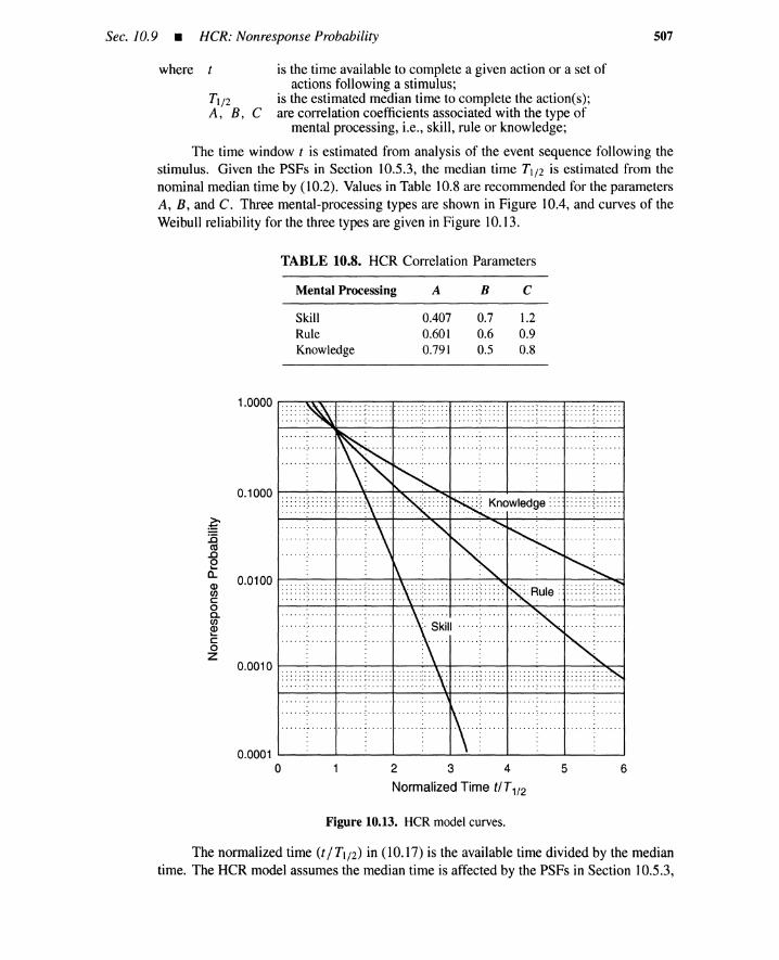
Sec. 10.9 • HCR: Nonresponse Probability 507
where is the time available to complete a given action or a set ofactions following a stimulus;
T1/ 2 is the estimated median time to complete the actiorus);A, B, C are correlation coefficients associated with the type of
mental processing, i.e., skill, rule or knowledge;
The time window t is estimated from analysis of the event sequence following thestimulus. Given the PSFs in Section 10.5.3, the median time T1/ 2 is estimated from thenominal median time by (10.2). Values in Table 10.8 are recommended for the parametersA, B, and C. Three mental-processing types are shown in Figure 10.4, and curves of theWeibull reliability for the three types are given in Figure 10.13.
TABLE 10.8. HCR Correlation Parameters
Mental Processing A B c
SkillRuleKnowledge
0.4070.6010.791
0.70.60.5
1.20.90.8
1.0000 r----..............--r----,.------,.----,.------,.-------,
0.1000
~:0«S
D0~
o,0.0100Q)
enc00.enQ)~
c0Z
0.0010...... : : : : ; : .
.. .. .. .. .. .....................................................................................
.. .. .. .. .. ..~ .. .. .. .. ..:.. .. .. .. .. .. .. .. .. .. .. .. .. .:.. .. .. .. .. .. .. .. .. .. .. .. ..:.. .. .. .. .. .. .. .. .. .. ..:.. .. .. .. .... ............:.........................:............
.. .. .. .. .. ..
6234 5
Normalized Time tlT1/2
.. "" ........ _ .
.. .. .. .. .. ..
.. .. .. .. .. .... .. .. .. .. .... .. .. .. .. .... .. .. .. .. ..0.0001 '--- ..L.--- ..L.--- --I
o
Figure 10.13. HeR model curves.
The normalized time (t / Tl/2) in (10.17) is the available time divided by the mediantime. The HCR model assumes the median time is affected by the PSFs in Section 10.5.3,

508 HUI11an Reliability _ Chap. 10
the HCR model curves' shapes vary according to the mental-processing type, and thenonresponse probability decreases in proportion to the normalized time (t / TI / 2) .
The foJlowing example describes an HCR application involving a single operatorresponse, that is, manual shutdown. Appendix A.2 presents a case with two responses inseries.
Example 23-Manual plant shutdown. A reactor is cooled by a heat exchanger. Con-sider as an initiating event loss of feedwater to the heat exchanger. This calls for a manual plantshutdown by the control room crew if the automatic-shutdown system fails. Suppose that the crewmust complete the plant shutdown within 79 s from the start of the initiating event. We have thefollowing information about the detection, diagnosis, and action phases.
1. Detection: The control panel information interface is good. The crew can easily see or hearthe feedwater-pump trip indicator, plant shutdown alarm, and automatic-shutdown failureannunciator. The nominal median time for detection is lOs.
2. Diagnosis: The instrumentation is such that the control room personnel can easily diagnosethe loss-of-feedwater accident and the automatic-shutdown failure, so a misdiagnosis is nota contributing statistical likelihood. The nominal median diagnosis time is 15 s.
3. Response: The control panel interface is good, so slip errors for the manual shutdown arejudged negligible. The nominal median response time is also negligible.
Table 10.9 summarizes the cognitive-processing type, PSFs, and nominal median time formanual shutdown.
TABLE 10.9. Manual Shutdown Characteristics
Task
Cognitive behaviorOperator experienceStress levelOperator/plant interface
Nominal median timeNominal median timeNominal median timeNominal median time
Manual shutdown
Skill (A = 0.407, B = 0.7, C = 1.2)Average (K] = 0.00)Potential emergency (K2 = 0.28)Good (KJ = 0.00)
lOs (detection)15 s (diagnosis)os (response)25 s (total)
The actual median response time (T]/2) for the manual shutdown is calculated by multiplyingthe 25-s nominal median time by the 1.28 stress level in Table 10.9:
T]/2 = I. 28 x 25 = 32 s
From the HCR model (10.17), using constants from Table 10.9:
[ {(79/32) - 0.7 } 1.2]
Pr{79} = exp - = 0.0029/demand0.407
(10.18)
(10.19)
If the stress is changed to its optimal level (e.g., K2 = 0), the nonresponse probability becomes0.00017/demand; if knowledge-based mental processing is required and the corresponding constantsare taken from Table 10.9, the HCR model yields 0.028/demand. In this example, only nonresponseprobability is considered. If lapse/slip errors during the response phase cannot be neglected, theseshould also be quantified by an appropriate method such as THERP. •

Sec. 10.10 • Wrong Actions Due to Misdiagnosis
10.10 WRONG ACTIONS DUE TO MISDIAGNOSIS
509
If a doctor does not prescribe an appropriate drug for a seriously hypertensive patient, hemakes a nonresponse failure; if the doctor prescribes a hypotensive drug for the wrongpatient, he commits an incorrect action. When unsuitable plans are formed during thediagnosis phase, the resultant actions are inevitably wrong. For a chess master, an incorrectplan results in a wrong move. The typical cause of a wrong action is misdiagnosis.
Because event trees are based on a binary logic, the failure branch frequently impliesa nonresponse. Because human behavior is unpredictable, there are an almost countlessnumber of wrong actions. Their inclusion makes the event-tree analysis far more complexbecause tree branches increase significantly. However, if we can identify typical wrongactions caused by initiating-event or procedure confusions, then event-tree analysis is sim-plified. In this section, the Wakefield [8] approach to misdiagnosis is described.
10.10.1 Initiating-Event Confusion
An approach to misdiagnosis based on confusion matrices is shown in Table 10.10.Each row or column represents an initiating event; a total of five initiating events areconsidered. Symbol L in row i and column j represents a likelihood that the row i initiatingevent is misdiagnosed as the column j initiating event; symbol C denotes the severity orimpact of this misdiagnosis. The likelihood and severity are usually expressed qualitativelyas high, medium, low, negligible, and so forth.
TABLE 10.10. Confusion Matrix
11 12 13 14 IS
II L12,C12 L13,C13 L14,C14 L15,C1512 L21,C21 L23,C23 L24,C24 L25,C2513 L31,C31 L32,C32 L34,C34 L35,C3514 L4I,C41 L42,C42 L43,C43 L45,C4515 L51,C5I L52,C52 L53,C53 L54,C54
Plant-response matrix. Information required for constructing the confusion matrixis the plant-response matrix shown in Table 10.11. Each row denotes an initiating event;each column represents a plant indicator such as a shutdown alarm. The symbols used areON: initiation of alarm; OFF: termination of signal; U: increase; D: decrease; X: increase ordecrease; 0: zero level. From this matrix, we can evaluate the likelihood of misdiagnosinginitiating events.
TABLE 10.11. Plant Response Matrix
Rl R2 R3 R4 RS R6
II ON OFF U D X 012 ON ON X U D D13 ON OFF D D 0 U14 OFF ON 0 X 0 015 OFF OFF D X U 0
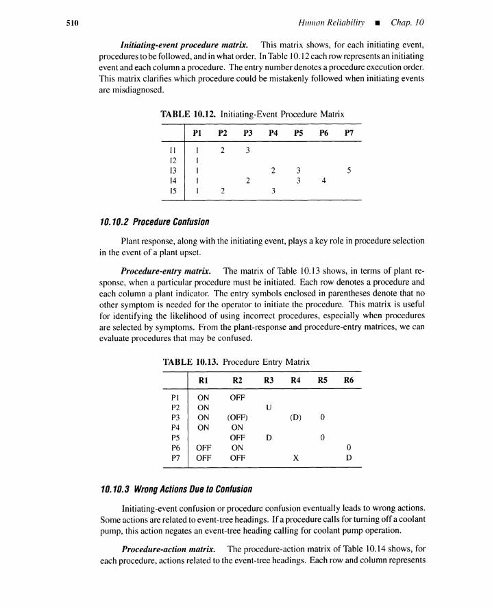
510 Human Reliability _ Chap. 10
Initiating-event procedure matrix. This matrix shows, for each initiating event,procedures to be followed, and in what order. In Table 10.12 each row represents an initiatingevent and each column a procedure. The entry number denotes a procedure execution order.This matrix clarifies which procedure could be mistakenly followed when initiating eventsare misdiagnosed.
TABLE 10.12. Initiating-Event Procedure Matrix
PI P2 P3 P4 P5 P6 P7
II 2 31213 2 3 514 2 3 415 2 3
10.10.2 Procedure Confusion
Plant response, along with the initiating event, plays a key role in procedure selectionin the event of a plant upset.
Procedure-entry matrix. The matrix of Table 10.13 shows, in terms of plant re-sponse, when a particular procedure must be initiated. Each row denotes a procedure andeach column a plant indicator. The entry symbols enclosed in parentheses denote that noother symptom is needed for the operator to initiate the procedure. This matrix is usefulfor identifying the likelihood of using incorrect procedures, especially when proceduresare selected by symptoms. From the plant-response and procedure-entry matrices, we canevaluate procedures that may be confused.
TABLE 10.13. Procedure Entry Matrix
Rl R2 R3 R4 R5 R6
PI ON OFFP2 ON UP3 ON (OFF) (D) 0P4 ON ONP5 OFF 0 0P6 OFF ON 0P7 OFF OFF X 0
10.10.3 Wrong Actions Due toConfusion
Initiating-event confusion or procedure confusion eventually leads to wrong actions.Some actions are related to event-tree headings. If a procedure calls for turning off a coolantpump, this action negates an event-tree heading calling for coolant pump operation.
Procedure-action matrix. The procedure-action matrix of Table 10.14 shows, foreach procedure, actions related to the event-tree headings. Each row and column represents
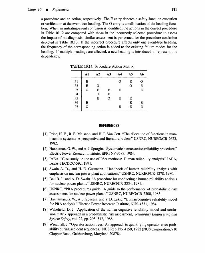
Chap. 10 • References 511
a procedure and an action, respectively. The E entry denotes a safety-function executionor verification at the event-tree heading. The 0 entry is a nullification of the heading func-tion. When an initiating-event confusion is identified, the actions in the correct procedurein Table 10.12 are compared with those in the incorrectly selected procedure to assessthe impact of misdiagnosis; similar assessment is performed for the procedure confusiondepicted in Table 10.13. If the incorrect procedure affects only one event-tree heading,the frequency of the corresponding action is added to the existing failure modes for theheading. If multiple headings are affected, a new heading is introduced to represent thisdependency.
TABLE 10.14. Procedure Action Matrix
Al A2 A3 A4 A5 A6
PI E 0 E 0P2 E 0 0 EP3 0 E E E EP4 0 EP5 E 0 E EP6 E E EP7 0 E E E
REFERENCES
[1] Price, H. E., R. E. Maisano, and H. P. Van Cotto "The allocation of functions in man-machine systems: A perspective and literature review." USNRC, NUREG/CR-2623,1982.
[2] Hannaman, G. W., and A. J. Spurgin. "Systematic human action reliability procedure."Electric Power Research Institute, EPRI NP-3583, 1984.
[3] IAEA. "Case study on the use of PSA methods: Human reliability analysis." IAEA,IAEA-TECDOC-592, 1991.
[4] Swain A. D., and H. E. Guttmann. "Handbook of human reliability analysis withemphasis on nuclear power plant applications." USNRC, NUREG/CR-1278, 1980.
[5] Bell B. J., and A. D. Swain. "A procedure for conducting a human reliability analysisfor nuclear power plants." USNRC, NUREG/CR-2254, 1981.
[6] USNRC. "PRA procedures guide: A guide to the performance of probabilistic riskassessments for nuclear power plants." USNRC, NUREG/CR-2300, 1983.
[7] Hannaman, G. W., A. J. Spurgin, and Y. D. Lukic. "Human cognitive reliability modelfor PRA analysis." Electric Power Research Institute, NUS-4531, 1984.
[8] Wakefield, D. J. "Application of the human cognitive reliability model and confu-sion matrix approach in a probabilistic risk assessment," Reliability Engineering andSystem Safety, vol. 22, pp. 295-312,1988.
[9] Wreathall, J. "Operator action trees: An approach to quantifying operator error prob-ability during accident sequences." NUS Rep. No. 4159, 1982 (NUS Corporation, 910Clopper Road, Gaithersburg, Maryland 20878).
512 HU111an Reliability _ Chap. 10
[10] Woods, D. D., E. M. Roth, and H. Pople, Jr. "Modeling human intention formationfor human reliability assessment," Reliability Engineering and System Safety, vol. 22,pp. 169-200, 1988.
[11] Hancock, P. A. "On the future of hybrid human-machine systems." In Verification andValidation of Complex Systems: Human Factors Issues, edited by Wise et al. Berlin:Springer-Verlag, 1993, pp. 61-85.
[12] Reason, J. "Modeling the basic error tendencies of human operators," ReliabilityEngineering and System Safety, vol. 22, pp. 137-153, 1988.
[13] Silverman, B. G. Critiquing Human Error-A Knowledge Based Human-ComputerCollaboration Approach. London: Academic Press, 1992.
[14] Hashimoto, K. "Human characteristics and error in man-machine systems," J. Societyoflnstrument and Control Engineers, vol. 19, no. 9, pp. 836-844, 1980 (in Japanese).
[15] Kuroda, I. "Humans under critical situations," Safety Engineering, vol. 18, no. 6, pp.383-385, 1979 (in Japanese).
[16] Rasmussen, J. Information Processing and Human-Machine Interaction: An Ap-proach to CognitiveEngineering. New York: North-Holland Series in System Scienceand Engi neering, 1986.
[17] Hollnagel, E. Human ReliabilityAnalysis: Contextand Control.New York: AcademicPress, 1993.
[18] Embrey, D. E. et al. "SLIM-MAUD: An approach to assessing human error probabil-ities using structured expert judgment." USNRC, NUREG/CR-3518, 1984.
[19] Apostolakis, G. E., V. M. Bier, and A. Mosleh. "A critique of recent models forhuman error rate assessment," Reliability Engineering and System Safety, vol. 22, pp.201-217, 1988.
[20] Hayashi, Y. "System safety," Safety Engineering, vol. 18, no. 6, pp. 315-321, 1979(in Japanese).
[21] Nakamura, S. "On human errors," Safety Engineering, vol. 18, no. 4, pp. 391-394,1979 (in Japanese).
[22] Kano, H. "Human errors in work," Safety Engineering, vol. 18, no. 4, pp. 186-191,1979 (in Japanese).
[23] Hashimoto, K. "Biotechnology and industrial society," Safety Engineering, vol. 18,no. 6, pp. 306-314, 1979 (in Japanese).
[24] Aoki, M. "Biotechnology and chemical plant accidents caused by operator error andits safety program (2)," Safety Engineering, vol. 21, no. 3, pp. 164-171, 1982 (inJapanese).
[25] Iiyama, Y. "A note on the safety of Shinkansen (JNR's high-speed railway)," SafetyEngineering, vol. 18, no. 6, pp. 360-366, 1979 (in Japanese).
[26] Kato, K. "Man-machine system and safety in aircraft operations," J. Society ofInstru-ment and Control Engineers, vol. 19, no. 9, pp. 859-865, 1980 (in Japanese).
[27] Aviation Week & Space Technology, April 7, 1975, pp. 54-59.
[28] Aviation Week & Space Technology, April 14, 1975, pp. 53-56.
[29] Furuta, H. "Safety and reliability ofman-machine systems in medical fields," J.SocietyofInstrument and Control Engineers, vol. 19, no. 9, pp. 866-874, 1980 (in Japanese).

Appendix A.l • THERP for Errors During a Plant Upset
CHAPTER TEN APPENDICES
A.1 THERP FOR ERRORS DURING APLANT UPSET
513
The following example shows THERP can be applied to defined-procedure tasks dur-ing plant upsets where diagnosis and time-pressure elements are relatively insignificant.THERP can also be extended to cases where time is limited; the techniques of WinslowTaylor may be modified to quantify human errors for defined-procedure tasks under timestress. The nonresponse HCR model in Section 10.9 considers the detection-diagnosis-response as a holistic process when a task analysis is infeasible.
Consider four tasks described in a procedure manual for responding to a small LOCA(loss of coolant accident) at a heat-generating reactor involving hazardous materials. Thereactor vessel is housed in a containment. The reactor pressure was high during the earlyaccident period, and the HPI (high-pressure injection) pumps have successfully started andsupplied coolant to the reactor.
Tasks in manual
1. Task 1. Monitor RC (reactor-coolant) pressure and temperature. Maintain atleast a 500P margin to saturation by holding RC pressure near the maximumallowable pressure of the cooldown pressure-temperature curve. The pressure canbecontrolled by manipulating heater switches for a pressurizer.
2. Task 2. When the RC margin to saturation becomes> 50oP, throttle HPI MOVs(motor-operated valves) to hold pressurizer water level at the setpoint. Initiateplant cooldown by Tasks 3 and 4 below at a rate that allows RC pressure to bemaintained within the cooldown pressure-temperature envelope.
3. Task 3. Switch from short-term HPI pumps to long-term LPI (low-pressure injec-tion) pumps.3.1. Verify that HPI tank outlet valve MU-13 for HPI is closed.3.2. Open valves DH-7A and DH-7B for LPI discharge to HPI pump suction,
verify that HPI suction crossover valves MU-14, MU-15, MU-16, and MU-17 are open, and verify that HPI discharge crossover valves MU-23, MU-24,MU-25, and MU-26 are open.
3.3. Go to basement 4 to close floor drain valves ABS-13 and ABS-14 and wa-tertight doors. Go to the third floor to close ventilation room purge dampersCV-7621, CV-7622, CV-7637, and CV-7638 from ventilation control panel(east wall of the ventilation room).
3.4. Verify that both LPI pumps are operating and LPI MOVs are open (MOV-1400and MOV-1401).
4. Task 4. Monitor the level in water storage tank (WST) that supplies water to theLPI pumps. When the WST level has fallen to 6 ft or when the corresponding low-level alarm is received, transfer the LPI pump suction to containment basementsump by verifying that the sump suction valves inside containment MOV-1414 andMOV-1415 are open. Open sump suction valves outside containment MOV-1405and MOV-1406, and then close both WST outlets MOV-1407 and MOV-1408.Close catalyst tank outlets MOV-1616 and MOV-1617, which supply water toanother safety system.

514 Human Reliability _ Chap. 10
As stated in the procedure manual, verify all actions and, if necessary, correct thestatus of a given item of equipment. For example, if the operator verifies that a valve shouldbe open and, on checking its status, finds it closed, it is opened manually.
Boundary conditions. In the talk-through (Step 3) in Figure 10.9, some generalinformation is gathered that relates to the performance of the four tasks.
1. The plant follows an emergency procedure in dealing with the small LOCA. It isassumed that the situation has been diagnosed correctly and that the operators havecorrectly completed the required precursor actions. The level of stress experiencedby the operators will be higher if they have already made prior mistakes. Task Iwill start approximately I hr after start of the LOCA.
2. At least three licensed operators are available to deal with the situation. One ofthem is the shift supervisor.
3. Tasks I, 2, 3.4, and 4 are performed in the control room, while Tasks 3.1, 3.2, and3.3 take place outside the control room.
4. Allocation of controls and displays are shown in Figure Al 0.1. The tasks areperformed on five different building levels-F3, FI, B2, B3, and B4.
Task analysis. In the task-analysis step depicted in Figure 10.9, we decompose thefour tasks into the unit activities shown in Table A 10.1. The symbols CB and ESFP in thelocation column denote a control board and emergency safety features panel, respectively.The 0 and C columns represent omission and commission errors, respectively. The errorlabels underlined in these two columns are the more serious ones.
In the human-reliability analysis that follows, we assume that three operators areinvolved: supervisory operator I, senior operator II, and junior operator III. Operator Iperforms activities required at the ESFP in the control room on the first floor. An exceptionis unit task 6 at CB. Operator II carries out the activities at the CB in the control roomand also goes to the ventilation room on the third floor to perform Task 3.3, activity 12.Operator III is in charge of activities on the basement levels; protective clothing must beworn. The allocation of operators to the unit activities are:
I: 5, 6, 14, 16, 17, 18, 19II: I, 2, 3, 4, 12, 15
III: 7, 8, 9, 10, I I, 13
The functions performed by operators I and II are summarized in the event tree ofFigure AIO.2, and those performed by operator III are modeled by Figure AIO.3.
Assigning BHEP. A-Omit monitoring: Activities I to 4 form a task group, thusprobability of an omission error applies to the entire task, and only by forgetting to performTask I will the operator forget to perform any element of it (see column 0 in Table Al 0.1).
Because we are dealing with the operator's following a set of written procedures, weuse an error estimate from Table A I0.6 (see page 530). This table presents estimates oferrors of omission made by operators using written procedures. These estimates reflect theprobability, under conditions stated, of an operator's omitting anyone item from a set ofwritten procedures. Because the procedures in this example are emergency procedures thatdo not require any step check-offby the operator, we use the section ofTable Al 0.6 that dealswith procedures having no check-off provision. Given that "omit monitoring" applies to a

Appendix A.l • THERP for Errors During a Plant Upset
F3Ventilation Room
Switches for CV-762I, 7622, 7637, 7638
F2
Control Room
Control Board ESF Panel
RC PressureChart Recorder Switchesfor 4 HPI MOVs
RC TemperatureDigital Indicator Indicatorsfor LPI PumpsCool-DownCurve Indicatorsfor MOV-1400, 1401
FIHeaterSwitches Switchesfor MOV-1400, 1401
WST-Level Indicator Indicatorsfor MOV-1414, 1415Switches for MOV-1414, 1415Switchesfor MOV-1405, 1406Switchesfor MOV-1407, 1408Switches for MOV-1616, 1617
Bl
B2UPI Pump Room
MU-13
LPI Pump Room
B3MU-14, IS, 16, 17MU-23,24, 25, 26DH-7A,DH-7B
B4 Rooms
B4 ABS-13,ABS-14
Watertight Doors
Equipment Description
CV-7621,CV-7622, Purge Dampers in Ventilation RoomCV-7637,CV-7638MOV-1400, MOV-1401 LPI MOVsMOV-1414, MOV-141S Sump Suction Valves InsideContainmentMOV-140S, MOV-1406 Sump Suction Valves OutsideContainmentMOV-1407, MOV-1408 WSTOutletsMOV-1616, MOV-1617 CatalystTank OutletsABS-13,ABS-14 B4 Floor Drain ValvesDH-7A, DH-7B LPI DischargeValvesto HPI Pump SuctionMU-14,MU-15, MU-16, MU-17 HPI PumpSuctionCrossoverValvesMU-23,MU-24, MU-25, MU-26 HPJ Pump DischargeCrossover ValvesMU-13 HPJTank Outlet
Figure AIO.I. Allocation of controls and displays.
515
long list of written procedures, its estimated HEP is 0.01 (0.005 to 0.05), as in item 5 ofTable Al0.6. The significance of the statistical error bounds is discussed in Chapter 11.
B-Pressure-reading error: The operator reads a number from a chart recorder. TableAIO.? (see page 530) presents estimated HEPs for errors made in reading quantitativeinformation from different types of display. For the chart recorder in question, item 3 fromthe table is used, 0.006 (0.002 to 0.02).
C-Temperature-reading error: This error involves reading an exact value from adigital readout; therefore, item 2 from Table AIO.? applies, 0.001 (0.0005 to 0.005).
D-Curve-reading error: This applies to activity 3. The HEP for errors made inreading quantitative information from a graph is used, item 4 from Table AID.?, 0.01(0.005 to 0.05).
Because feedback from manipulating heater switches incorrectly is almost immediate,the probability of making a reversal error during activity 4 is not considered.

516
TABLE AIO.I. A Task Analysis Table
Human Reliability _ Chap. 10
UnitTask Task Description Location Operator 0 C
Task I I Read RC pressure chart (analog) FI,CB II A !!2 Read RC temperature (digital) FI, CB II A C3 Read pressure-temperaturecooldown curve on a FI,CB II A D
tape4 Manipulate pressurizerheater switches to control FI,CB II A
the pressure and temperature
Task 2 5 Throttle four HPI MOVs FI, ESFP I E G6 Initiatecooldown (Tasks3 and 4) followingwrit- FI,CB I u
ten procedures
Task 3.1 7 Verify MU-13 (closed) B2 III T,U
Task 3.2 8 Open DH-7A and DH-7B B3 III T,V9 VerifyMU-14, MU-15, MU-16, and MU-17 B3 III T,V
(open)10 VerifyMU-23, MU-24, MU-25, and MU-26 B3 III T,V
(open)
Task 3.3 II Close ABS-13 and ABS-14 B4 III T,W12 Close CV-762I, CV-7622,CV-7637,and CV- F3 II I J}-J4
7638
13 Close watertight doors B4 III T,W
Task 3.4 14 Verifythat both LPI pumps are on and that FI, ESFP I K L},M}
MOV-1400 and MOV-140I are open FI, ESFP I K L2,M2
Task 4 15 Monitor WST level FI,CB II N 016 VerifyMOV-1414 and MOV-1415 (open) FI, ESFP I ~ Pl,Q17 Open MOV-1405 and MOV 1406 FI, ESFP I ~ f2,B218 Close MOV-1407 and MOV-1408 FI, ESFP I ~ P3, R319 Close MOV-1616 and MOV-1617 FI, ESFP I ~ P4, R4
E-Omit throttling HPI MOVs: There are four switches for four HPI MOVs on thevertical ESFP on the first floor control room. For the operator, throttling four HPI MOV s
is a unit activity. Therefore, probability of an omission error applies to them all. The same
HEP used for omission error A, 0.01 (0.005 to 0.05), is used.
G-Incorrectly select fourth MOV: The four HPI MOVs on the panel are delineatedwith colored tape; therefore, a group selection error is very unlikely. However, it is known
that a similar switch is next to the last HPI MOV control on the panel. Instead of MOVs 1,
2, 3, and 4, the operator may err, and throttle MOVs 1, 2, 3, and the similar switch. Table
AI0.8 (see page 531) contains HEPs for errors of commission in changing or restoring
valves. Because item 7 most closely approximates the situation described here, an HEP of
0.003 (0.00 1 to 0.01) applies.H-Omit initiating cooldown: This applies to unit activity 6. The error is one of
omission of a single step in a set of written procedures, so 0.01 (0.005 to 0.05) in TableAI0.6 is used. Activities 7 to II are performed on basement levels by operator III, so we
next consider activity 12 as performed by operator lIon the third floor.

Appendix A.l • THERP for Errors During a Plant Upset 517
R3 : Reversal ErrorMOVs 1407,1408
0: WST ReadingError
P1: Selection ErrorMOVs 1414,1415
A: OmitMonitoring
B: Pressure-ReadingError
c:Temperature-ReadingError
E: Omit ThrottlingHPI MOVs
0: Curve-ReadingError
G: Selection Error4th MOV
H: Omit InitiatingCooldown
I: Omit ClosingDampers
J1: Selection ErrorCV-7621
J2: Selection ErrorCV-7622
J 3: Selection ErrorCV-7637
J4:Selection ErrorCV-7638
K: Omit Verifying LPIPumps and MOVs
L1: Selection ErrorLPI Pumps
L2 : Selection ErrorLPI MOVs
M1: Interpretation ErrorLPI Pumps
M2 : Interpretation ErrorLPI MOVs
N: Omit RespondingtoWST
Q: Interpretation ErrorMOVs 1414,1415
P2 : Selection ErrorMOVs 1405,1406
R2 : Reversal ErrorMOVs 1405,1406
P3: Selection ErrorMOVs 1407,1408
P4: Selection ErrorMOVs 1416,1417
R 4: Reversal ErrorMOVs 1416,1417
e: ThrottleHPI MOVs
d: Read CurveCorrectly
b: Read PressureCorrectly
c: Read TemperatureCorrectly
a: PerformMonitoring
g: Select 4th MOVCorrectly
h: InitiateCooldown
i: CloseDampers
j1: Select CV-7621Correctly
j2: Select CV-7622Correctly
j3: Select CV-7637Correctly
k: Verify LPIPumps and MOVs
n: Respond toWST
m1: Interpret LPI PumpsCorrectly
' 2: Select LPI MOVsCorrectly
j4: Select CV-7638Correctly
' 1: Select LPI PumpsCorrectly
m2: Interpret LPI MOVsCorrectly
0: Read WSTCorrectly
P1: Select MOVs1414,1415 Correctly
q: Interpret MOVs1414,1415 Correctly
P2: Select MOVs1404,1406 Correctly
'2: Operate MOVs1405,1406 Correctly
P3: Select MOVs1407,1408 Correctly
'3: Operate MOVs1407,1408 Correctly
P4: Select MOVs1416,1417 Correctly
'4: Operate MOVs1416,1417 Correctly
Figure AI0.2. HRA event tree for operators I and II in the control room.
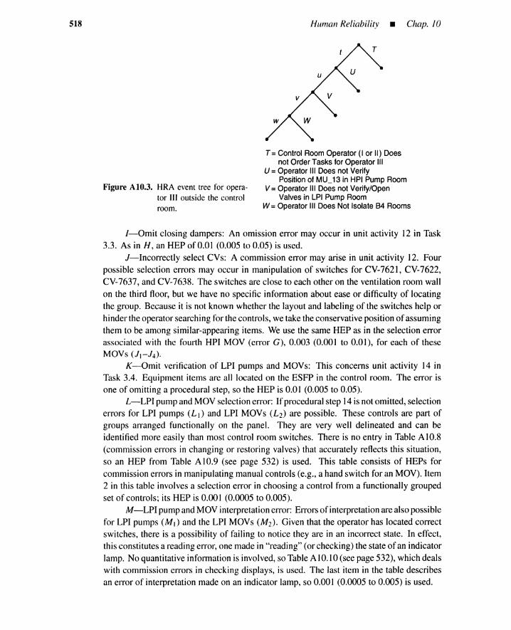
518 Human Reliability _ Chap. 10
T
v
Figure AI0.3. HRA event tree for opera-tor III outside the controlroom.
T = ControlRoom Operator(lor II) Doesnot OrderTasks for OperatorIII
U=OperatorIII Doesnot VerifyPosition of MU_13in HPI PumpRoom
V =OperatorIII Doesnot Verify/OpenValvesin LPI PumpRoom
W= OperatorIII DoesNot Isolate84 Rooms
I-Omit closing dampers: An omission error may occur in unit activity 12 in Task3.3. As in H, an HEP of 0.01 (0.005 to 0.05) is used.
i-Incorrectly select CVs: A commission error may arise in unit activity 12. Fourpossible selection errors may occur in manipulation of switches for CV-7621, CV-7622,CV-7637, and CV-7638. The switches are close to each other on the ventilation room wallon the third floor, but we have no specific information about ease or difficulty of locatingthe group. Because it is not known whether the layout and labeling of the switches help orhinder the operator searching for the controls, we take the conservative position ofassumingthem to be among similar-appearing items. We use the same HEP as in the selection errorassociated with the fourth HPI MOV (error G), 0.003 (0.001 to 0.01), for each of theseMOVs (J}-J4 ) .
K-Omit verification of LPI pumps and MOVs: This concerns unit activity 14 inTask 3.4. Equipment items are all located on the ESFP in the control room. The error isone of omitting a procedural step, so the HEP is 0.01 (0.005 to 0.05).
L-LPI pump and MOV selection error: If procedural step 14 is not omitted, selectionerrors for LPI pumps (L}) and LPI MOVs (L2) are possible. These controls are part ofgroups arranged functionally on the panel. They are very well delineated and can beidentified more easily than most control room switches. There is no entry in Table AIO.8(commission errors in changing or restoring valves) that accurately reflects this situation,so an HEP from Table Al 0.9 (see page 532) is used. This table consists of HEPs forcommission errors in manipulating manual controls (e.g., a hand switch for an MOV). Item2 in this table involves a selection error in choosing a control from a functionally groupedset of controls; its HEP is 0.00 1 (0.0005 to 0.005).
M-LPI pump and MOV interpretation error: Errors of interpretation are also possiblefor LPI pumps (M}) and the LPI MOVs (M2) . Given that the operator has located correctswitches, there is a possibility of failing to notice they are in an incorrect state. In effect,this constitutes a reading error, one made in "reading" (or checking) the state of an indicatorlamp. No quantitative information is involved, so Table A 10.10 (see page 532), which dealswith commission errors in checking displays, is used. The last item in the table describesan error of interpretation made on an indicator lamp, so 0.001 (0.0005 to 0.005) is used.

Appendix A.l • THERP for Errors During a Plant Upset 519
N-Omit responding WST: This applies to unit activities 15 to 19 in Task 4. If theoperator omits responding to (or monitoring) the WST level, other activities in Task 4 willnot be performed. The same omission HEP used previously, 0.01 (0.005 to 0.05), applies.
O-WST reading error: An error in reading the WST meter could be made withoutthe omission error in N. If it is read incorrectly, other activities in Task 4 will not beperformed. Going back to Table AI0.7 for commission errors made in reading quantitativeinformation, the HEP to use in reading an analog meter is 0.003 (0.001 to 0.01), the firstitem in the table.
P-MOV selection error: This applies to unit activities 16 to 19. Errors PI, P2, P3,
and P4 involve selecting a wrong set of MOV switches from sets of functionally groupedswitches on the ESFP. As in L, this HEP is from Table AI0.9, 0.001 (0.0005 to 0.(05).
Q-MOVs 1414, 1415 interpretation error: This concerns unit activity 16 in Task 4.An interpretation error could be made in checking the status of an indicator lamp. An HEPof 0.001 (0.0005 to 0.005) is assigned.
R-MOV reversal error: There are three possible errors, R2, R3, and R4, for unitactivities 17, 18, and 19, respectively. Instead of opening valves, the operator might closethem or vice versa. The switches are on the ESFP. Because errors of commission for valve-switch manipulations are involved, Table Al 0.9 is used. Item 7 most closely describes thiserror; hence an HEP of 0.001 (0.0001 to 0.1).
Let us next consider the event tree for the task performed by operator III. The unitactivities are 7 to 11 and 13. Figure AIO.3 shows the event tree.
T-Control room operator omits ordering task: Activities 7 to 11and 13are performedoutside the control room. If operator I forgets to order operator III to perform this set ofactivities, this constitutes failure to carry out plant policy. An HEP of 0.01 (0.005 to 0.05)from Table A 11.11 (see page 532), item 1, is used.
U-Omit verifying MU-13: This involves unit activity 7 in Task 3.1. As shownin Figure AIO.1 and Table AI0.1, activity 7 is performed on the second-floor basement;activities 8,9, and 10 are carried out on basement 3; and activities 11 and 13 on basement4. Operator III sees these as three distinct unit tasks, one on each of three levels. Weassume that the operator will not be working from a set of written procedures but from oralinstructions from supervisory operator I in the control room. Data for this model are foundin Table Al 0.12 (see page 533). Operator III must recall three tasks, so we use item 3 inthe table, which shows an HEP of 0.01 (0.005 to 0.05) for each task.
Valve MU-13 is a manual valve on basement 2 and no selection error is possible. Itis not deemed likely that the operator will make a reversal error in this situation.
V-Omit to verify/open valves in LPI pump room: This involves unit activities 8, 9,and 10, which are viewed as a unit task performed in the LPI pump room of basement 3. Asstated in A, an HEP of 0.01 (0.005 to 0.05) is used. Neither a selection error nor a reversalerror is deemed likely.
W-Omit isolating B4 rooms: These are omission errors for unit activities 11 and 13.An HEP of 0.01 (0.005 to 0.05) was assumed, as in U and V. Valves ABS-13 and ABS-14are large, locally operated valves in basement 4. They are the only valves there. Similarly,there is only one set of watertight doors. Again, neither selection nor reversal errors areconsidered likely.
Evaluating PSFs. As described in Section 10.8.2, global PSFs affect the entiretask, whereas local PSFs affect only certain types of errors. Nominal HEPs in Handbook

520 Human Reliability _ Chap. 10
tables consider these local PSFs. We next consider the effect of global PSFs-those thatwill affect all HEPs. As stated in the original assumptions, the operators are experienced,and because they are following an emergency procedure, they are under a moderately highlevel of stress. We see from Table 10.2 that the HEPs for experienced personnel operatingunder a moderately high stress level should be doubled for discrete tasks and multiplied by5 for dynamic tasks.
Figure A I0.2 is the HRA event tree for control room actions for which the nominalHEPs in Table A 10.2 apply. The only dynamic tasks in this table are those calling formonitoring activities: the monitoring of the RC temperature and pressure indicators (unitactivities I and 2), the interpretation of these values (activities 3 and 4), and the WSTlevel monitoring (activity 15). Hence nominal HEPs, B, C, D, and 0 in Table AI0.2 aremultiplied by 5 to yield new HEPs; those for other events in the table are doubled.
Another overriding PSF that must be considered is the effect of operator Ill's havingto wear protective clothing. The first error T takes place in the control room. The HEPs T,U, V, and W must be doubled to reflect effects of moderately high stress levels. HEPs U,V, and W must be doubled again to reflect the effects of the protective clothing. The newHEPs are shown in Table A 10.3.
Assessing dependence. Several cases of dependence have already been accountedfor (see Table A I0.1 ).
(A.I)new A
1. Omission error A: This omission applies to tasks consisting of activities 1 to 4.2. Omission error E: For errors of omission, the four HPI MOVs are completely
dependent.
3. Commission error G: The first three HPI MOVs are free of selection errors, whilethe fourth is susceptible.
4. Omission error H: For errors of omission, steps in the cooldown procedures arecompletely dependent.
5. Omission error I: The four CVs are completely dependent with respect to theomission error,
6. Omission error N: Unit activities 15 to 19 are completely dependent.
7. Commission error 0: The same dependence as in case 6 exists for this readingerror,
8. Omission error T: The omission applies to the task consisting of activities 7 to IIand 13.
9. Omission errors U, V, and W: Each set of activities performed on a plant level iscompletely dependent with respect to omission.
The presence of operators I and II in the control room constitutes a recovery (orredundancy) factor with a high dependence between the two operators. Equation (10.8)indicates that an error is caught by another operator about half the time; this is a form ofhuman redundancy.
Table A 10.2 shows the HEPs as modified to reflect the effects of dependence. Prob-abilities of error for the two operators have been collapsed into a single limb for each typeof error. For instance, HEP A is modified in the following way.
(old A)[1 + (old A)]
2(0.02)(1 + 0.02) == 0.0102
2
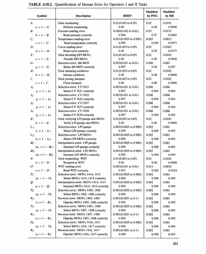
TABLE AIO.2. Quantification of Human Error for Operators I and II Tasks
Modified ModifiedSymbol Description BHEP by PSFs byHD
A: Omit monitoring 0.0 I (0.005 to 0.05) 0.02 0.0102
a = I-A: Perform monitoring 0.99 0.98 0.9898B: Pressure-reading error 0.006(0.002 to 0.02) 0.03 0.0155
b= 1- B: Read pressure correctly 0.994 0.97 0.9845
C: Temperature-reading error 0.00 I (0.0005 to 0.005) 0.005 0.0025
c= l-C: Read temperature correctly 0.999 0.995 0.9975
D: Curve-reading error 0.0 I (0.005 to 0.05) 0.05 0.0263
d= I-D: Read curve correctly 0.99 0.95 0.9737E: Omit throttling HPI MOVs 0.01 (0.005 to 0.05) 0.02 0.0102
e= 1- E: Throttle HPI MOVs 0.99 0.98 0.9898G: Selection error: 4th MOV 0.003(0.00 I to 0.0 I) 0.006 0.003
g = I-G: Select 4th MOV correctly 0.997 0.94 0.997H: Omit initiating cooldown 0.0 I (0.005 to 0.05) 0.02 0.0102
h = I-H: Initiate cooldown 0.99 0.98 0.9898J: Omit closing dampers 0.0 I (0.005 to 0.05) 0.02 0.0102
i = 1- J: Close dampers 0.99 0.98 0.9898
Jt: Selection error: CV-7621 0.003(0.00 I to 0.01) 0.006 0.006
h = 1- Jt: Select CV-762I correctly 0.997 0.994 0.994
J2: Selection error: CV-7622 0.003(0.00 I to 0.0 I) 0.006 0.006
l: = I - J2: Select CV-7622 correctly 0.997 0.994 0.994
J3: Selection error: CV-7637 0.003(0.00 I to 0.0 I) 0.006 0.006
ls = 1- J3: Select CV-7637 correctly 0.997 0.994 0.994
J4: Selection error: CV-7638 0.003(0.001 to 0.01) 0.006 0.006
j4 = 1 - J4: Select CV-7638 correctly 0.997 0.994 0.994K: Omit verifying LPI pumps and MOVs 0.01(0.005 to 0.05) 0.02 0.0102
k= 1- K: Verify LPI pumps and MOVs 0.99 0.98 0.9898t.; Selection error: LPI pumps 0.00 I(0.0005 to 0.005) 0.002 0.001
It = I-Lt: Select LPI pumps correctly 0.999 0.998 0.999
L2: Selection error: LPI MOVs 0.00 I(0.0005 to 0.005) 0.002 0.001
12 = 1 - L2: Select LPI MOVs correctly 0.999 0.998 0.999Mt: Interpretation error: LPI pumps 0.001(0.0005 to 0.005) 0.002 0.001
mt = I-Mt: Interpret LPI pumps correctly 0.999 0.998 0.999M2: Interpretation error: LPI MOVs 0.001 (0.0005 to 0.005) 0.002 0.001
m2 = 1- M2: Interpret LPI MOVs correctly 0.999 0.998 0.999N: Omit responding: WST 0.01 (0.005 to 0.05) 0.02 0.0102
n = I-N: Respond to WST 0.99 0.98 0.98980: WST reading error 0.003(0.00 I to 0.0 I) 0.015 0.0076
0= 1- 0: Read WST correctly 0.997 0.985 0.9924Pt: Selection error: MOVs 1414, 1415 0.001 (0.0005 to 0.005) 0.002 0.001
Pt = I- Pt : Select MOVs 1414, 1415 correctly 0.999 0.998 0.999Q: Interpretation error: MOVs 1414, 1415 0.001 (0.0005 to 0.005) 0.002 0.001
q = 1- Q: Interpret MOVs 1414, 1415 correctly 0.999 0.998 0.999P2: Selection error: MOVs 1405, 1406 0.001 (0.0005 to 0.005) 0.002 0.001
P2 = 1- P2: Select MOVs 1405, 1406 correctly 0.999 0.998 0.999R2: Reversal error: MOVs 1405, 1406 0.001 (0.000 I to 0.1) 0.002 0.001
rz = I - R2: Operate MOVs 1405, 1406 correctly 0.999 0.998 0.999P3: Selection error: MOVs 1407, 1408 0.00 I(0.0005 to 0.005) 0.002 0.001
P3 = 1- P3: Select MOVs 1407, 1408 correctly 0.999 0.998 0.999R3: Reversal error: MOVs 1407, 1408 0.00 I (0.000 I to 0.1) 0.002 0.001
r3 = 1 - R3: Operate MOVs 1407, 1408 correctly 0.999 0.998 0.999P4: Selection error: MOVs 1416, 1417 0.001(0.0005 to 0.005) 0.002 0.001
P4 = 1- P4: Select MOVs 1416, 1417 correctly 0.999 0.998 0.999R4: Reversal error: MOVs 1416, 1417 0.001 (0.0001 to 0.1) 0.002 0.001
r4 = 1- R4: Operate MOVs 1416, 1417 correctly 0.999 0.998 0.999
521

522 HU111an Reliability _ Chap. 10
TABLE AIO.3. Quantification of Human Error for Operators III Tasks
Modified ModifiedSymbol Description BHEP by PSFs byHD
T: Omit ordering tasks 0.0 I(0.005 to 0.05) 0.02 0.0102f == I - T: Order tasks 0.99 0.98 0.9898
U: Omit verifying MU- I3 in HPI pump room 0.0 I(0.005 to 0.05) 0.04 0.04
u == I - U: Verify MU- I3 correctly 0.99 0.96 0.96V: Omit verifying/opening valves in LPI pump room 0.0 I(0.005 to 0.05) 0.04 0.04
v == I - V: Verify/open valves in LPI pump room 0.99 0.96 0.96W: Omit isolating 84 rooms 0.0 I(0.005 to 0.05) 0.04 0.04
w == 1- W: Isolate 84 rooms correctly 0.99 0.96 0.96
Error J occurs in the third-floor ventilation room. In this case there is no dependencebetween the two operators because operator II goes to the room alone. The only event inTable A I0.3 that is dependent is the first (i.e., T). If operator I forgets to order these tasks,operator II may prompt him:
(old T)[I + (old T)]new T == --------
2(0.02)(1 + 0.02) == 0.0102
2
(A.2)
Determining success and failure probabilities. Once human-error events havebeen identified and individually quantified as in Tables A 10.2 and Al 0.3, their contributionto the occurrence and non-occurrence of the basic event must be determined. Assume that,as indicated by underlined letters in Table A 10.1, the paths ending in the nine error eventsA, B, C, D, H, N, 0, P2, R2 are failure nodes. The event tree in Figure AIO.2 can besimplified to Figure A I0.4 if we collapse the limbs that do not contribute to system failure.The probability of each failure node can be calculated by multiplying the probabilities onthe limbs of Figure A I0.4. For instance, the path ending at node F3 is
(0.9898)(0.98455)(0.0025) == 0.0024
The occurrence probability of system failure is thus
Pr{F} == 0.0102 + 0.0153 + 0.0024 + 0.0255 + 0.0097 + 0.0096 + 0.0070
+ 0.0009 + 0.0009 == 0.0815
(A.3)
(A.4)
Figure A I0.4 is suitable for further analysis because it shows the relative contribution ofevents to system failure.
A similar decision was made with respect to the HRA event tree in Figure AI0.3. Itwas decided that all paths terminating in human errors caused system failure.
Determining effects ofrecovery factors. Consider, for instance, omission error N.The operator should respond to the WST level's falling to 6 ft. Even if he forgets to monitorthe level indicators, there is still a possibility that the low-level alarm (annunciator) willremind him of the need for follow-up actions. We will treat the alarm as an alerting cueand analyze its effect as a recovery factor. Table Al 0.13 (see page 533) lists HEPs forfailing to respond to annunciating indicators. Assume that ten annunciators are alarmingthe accident. The probability of the operator's failing to respond to anyone of these tenis 0.05 (0.005 to 0.5). Figure A 10.5 shows the diagram for this recovery factor. Note that
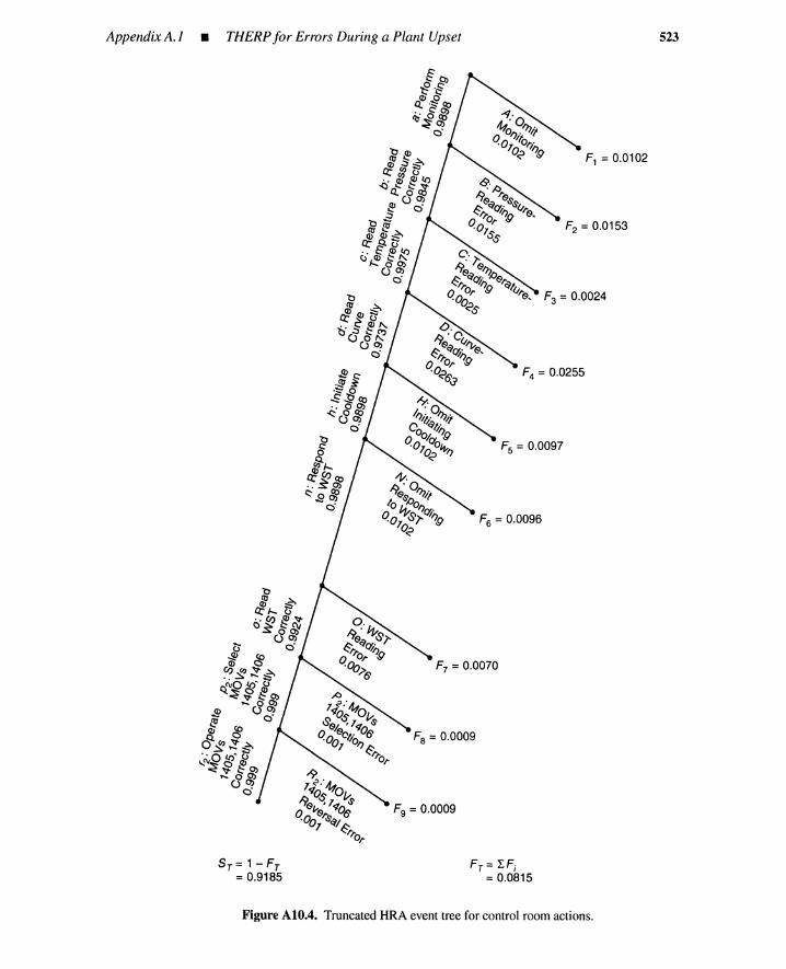
Appendix A.l • THERP for Errors During a Plant Upset
Fs = 0.0097
Fs =0.0096
F1 =0.0102
F2 = 0.0153
523
Sr= 1-Fr=0.9185
Fr = zr,=0.0815
Figure AIO.4. TruncatedHRA event tree for control room actions.

524
Sr = 1 - Fr=0.9275
Human Reliability _ Chap. 10
F1 = 0.0102
F2 =0.0153
F3 =0.0024
F4 = 0.0255
Fs =0.0005
F7 =0.0071
Fa = 0.0009
Fg =0.0009
Fr = 'LF;=0.0725
Figure AIO.5. Control room HRA event tree includingone recovery factor.

Appendix A.2 • HeRfor Two Optional Procedures 525
its inclusion in the analysis decreases the probability of total system failure from 0.0815 to0.0725. If this is an adequate increase, no more recovery factors are considered.
Sensitivity analysis. In this problem the two most important errors, in terms oftheir high probability, are errors Band D-reading the RC pressure chart recorder andpressure-temperature curve. For RC pressure, if the display were a digital meter instead ofa chart recorder, we see from Table AIO.7 that this would change the basic HEP for thattask from 0.006 (0.002 to 0.02) to 0.001 (0.0005 to 0.005). This new HEP must be modifiedto 0.005 (0.0025 to 0.025) to reflect effects of stress for dynamic tasks, and then modifiedagain to reflect the effect of dependence, thus becoming 0.0025 (0.001 to 0.01). Using0.0025 instead of 0.0155 results in a total-system-failure probability of 0.0604 as opposedto 0.0725.
To make the same sort of adjustment for error D, we redesign the graph so that it iscomparatively easy to read. If we use the lower bound of the HEP in Table A10.7, item 4,instead of the nominal value, we have 0.005. This becomes 0.025 when modified for stressand 0.0128 when modified for human redundancy.
An HRA event tree with these new values is shown in Figure Al 0.6. Total-system-failure probability becomes 0.0475. Whether this new estimate of the probability of systemfailure is small enough to warrant incorporating both changes is a management decision.
A.2 HCR FOR TWO OPTIONAL PROCEDURES
Consider again the initiating event "loss of feedwater to a heat exchanger." Time datafor relevant cues are given in Table Al 0.4. Assume that the plant has been shut downsuccessfully, and that heat from the reactor must now be removed. Because of the loss offeedwater, the heat-exchanger water level continuously drops. The low-water-Ievel alarmssound at 20 min after the start of the initiating event. Fortunately, a subcooling marginis maintained until the heat exchangers dry out; 40 min will elapse between the low-levelalarms and the heat exchangers emptying. The operators have 60 min before damage to thereactor occurs. Operators have two options for coping with the accident.
TABLE AIO.4. Time Data for Relevant Cues
Time
20 min40 min50 min60 min1 min
Remark
HEX alarmFrom HEX alarm to dry-outPORVs openTo fuel damageSwitch manipulation
1. Recovery of feedwater: The heat is removed by heat exchangers cooled by thefeedwater. This is called a secondary heat-removal recovery.
2. Feed and bleed: The operators manually open reactor PORVs (pressure-operatedrelief valves) to exhaust heat to the reactor containment housing. Because the hotsteam flows through the PORVs, the operators must activate the HPI to maintainthe coolant inventory in the reactor. The combination of PORV open operation

526 Human Reliability _ Chap. 10
Z = 0.0093
Fa =0.0010
F1 = 0.0102
F2 =0.0025
F3 =0.0025
F4 =0.0126
Fs =0.0099
Fs = 0.0005
Sr = 1 - Fr=0.9525
Fr= rF;= 0.0425
Figure AIO.6. HRA event tree for control room actions by operators I and II,with Tasks2 and 4 modified.
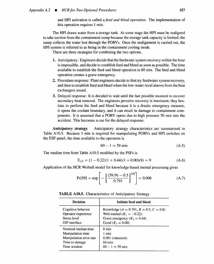
Appendix A.2 • HeR for Two Optional Procedures 527
and HPI activation is called afeed and bleed operation. The implementation ofthis operation requires 1 min.
The HPI draws water from a storage tank. At some stage the HPI must be realignedto take suction from the containment sump because the storage tank capacity is limited; thesump collects the water lost through the PORVs. Once the realignment is carried out, theHPI system is referred to as being in the containment cooling mode.
There are three strategies for combining the two options.
1. Anticipatory: Engineers decide that the feedwater system recovery within the houris impossible, and decide to establish feed and bleed as soon as possible. The timeavailable to establish the feed and bleed operation is 60 min. The feed and bleedoperation creates a grave emergency.
2. Procedure response: Plant engineers decide to first try feedwater system recovery,and then to establish feed and bleed when the low-water-Ievel alarms from the heatexchangers sound.
3. Delayed response: It is decided to wait until the last possible moment to recoversecondary heat removal. The engineers perceive recovery is imminent; they hes-itate to perform the feed and bleed because it is a drastic emergency measure,it opens the coolant boundary, and it can result in damage to containment com-ponents. It is assumed that a PORV opens due to high pressure 50 min into theaccident. This becomes a cue for the delayed response.
Anticipatory strategy. Anticipatory strategy characteristics are summarized inTable AIO.5. Because I min is required for manipulating PORVs and HPJ switches onthe ESF panel, the time available to the operators is
60 - 1 == 59 min
The median time from Table A10.5 modified by the PSFs is
TI / 2 == (I - 0.22)(1 + 0.44)(1 + 0.00)(8) == 9
(A.5)
(A.6)
(A.7)
Application of the HeR Weibull model for knowledge-based mental processing gives
[ {(59/9) - 0.5 }O.8]
Pr{59} == exp - == 0.0060.791
TABLE AlO.S. Characteristics of Anticipatory Strategy
Decision
Cognitive behaviorOperatorexperienceStress levelOIP interface
Nominalmedian timeManipulation timeManipulation error rateTime to damageTime window
Initiate feed and bleed
Knowledge (A = 0.791, B = 0.5, C = 0.8)Well-trained (K} = -0.22)Graveemergency (K2 = 0.44)Good (K3 = 0.00)
8 min1 min0.001 (omission)60 min60 - 1 = 59 min

528 HUI11an Reliability _ Chap. 10
Because the HEP for manipulationof PORVs and HPJis 0.001, the feed and bleed operationerror becomes
0.006 + 0.001 == 0.007 (A.8)
(A.9)
The successful feed and bleed (probability 0.993) must be followed by containmentcooling mode realignment. Alignment failure is analyzed by the human-reliabilityfault treeof Figure Al 0.7. The leftmost basic event "screening value" denotes a recovery failure.The operator must close a suction valve at the storage tank to prevent the HPJ pumps fromsucking air into the system. The operator must open a new valve in a suction line from thecontainment sump. The realignment-failureprobability is calculated to be 0.0005. Thus thetotal failure probability for the feed and bleed followed by the realignmentconsists of non-response probability, manipulation-failureprobability, and realignment-failureprobabilitywhen the preceding two failures do not occur:
Pr{Anticipatory strategy failure} == 0.006 + 0.001 + (1 - 0.007) x 0.0005
== 0.0075
Failureto Align
Heat-RemovalValve
System
Failureto RecoverIncorrect
ValveAlignment
IncorrectHeat-Removal
ValveAlignment
0.1Screening V_a_lu_e_..-IIoooo.-__......
Failureto FollowProcedure
Failureto ManipulateHeat-Removal
Valves
0.001HandbookValue
Failureto Open
NewSuctionValves
0.003HandbookValue
Failureto Close
OldSuctionValve
0.001HandbookValue
Figure AIO.7. Human-reliability fault tree for coolant realignment.

AppendixA.2 • HCRfor Two OptionalProcedures 529
Procedure-response strategy. The engineers first decide to recover the feedwatersystem. The feedwater-system recovery fails by hardware failures or human error, withprobability 0.2. Because the operators try to recover the secondary cooling during the first20 min until the heat exchanger low-water-Ievel alarm, the time available for the feed andbleed operation is
A.I060 - 20 - I == 39 (A.IO)
With respect to the feed and bleed operation, only this time window is specific to theprocedure response strategy; other characteristics remain the same as for the anticipatorystrategy. Thus the nonresponse probability for the feed and bleed is
[ {(39/9) - 0.5 }Oo8]
Pr{39} == exp - == 0.0290.791
(A. I I)
Because the feed and bleed manipulation failure probability is 0.001, the failure probabilityof feed and bleed is 0.03.
This strategy fails when the following happens.
1. The feedwater recovery fails due to hardware failures or human error (probability0.2), and the feed and bleed fails (probability 0.03).
2. The feedwater recovery fails (0.2), the feed and bleed succeeds (I - 0.03 == 0.97),and the realignment activity fails (0.0005).
As a result, the procedure response strategy fails with probability
Pr{Procedure-response strategy failure} == (0.2)(0.03) + (0.2)(0.97)(0.0005)
== 0.007(A.12)
Delayed-response strategy. The engineers first decide to recover the feedwatersystem. The feed and bleed cue is set off at 50 min when a PORV opens. Thus theengineers only have 10 - 1 == 9 min for the feed and bleed decision. Assume rule-basedmental processing and a nominal median time of 3 min. Then the actual median timebecomes
T1/ 2 == 3 x 1.44 x 0.78 == 3.4
The nonresponse probability is now
P {9}[ {
(9/3.4) - 0.6 }Oo9]r == exp - == 0.049
0.601
(A.13)
(A.14)
Because the manual failure probability is 0.00 I, the feed and bleed failure probability is0.049 + 0.001 ~ 0.05. This strategy fails in the following cases.
1. The feedwater system recovery fails due to hardware failures or human errors(estimated probability 0.05 because more time is available than in the procedure-response case), and the feed and bleed fails (probability 0.05).
2. The feedwater system recovery fails (0.05), the feed and bleed succeeds (1-0.05 ==0.95), and the realignment activity fails (0.0005).
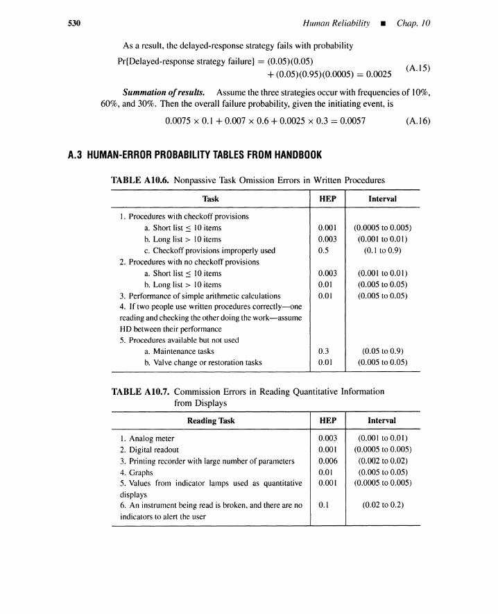
530 HU111an Reliability _ Chap. 10
As a result, the delayed-response strategy fails with probability
Pr{Delayed-response strategy failure} == (0.05)(0.05)
+ (0.05)(0.95)(0.0005) == 0.0025(A.I5)
Summation ofresuits. Assume the three strategies occur with frequencies of 10%,60%, and 30%. Then the overall failure probability, given the initiating event, is
0.0075 x 0.1 + 0.007 x 0.6 + 0.0025 x 0.3 == 0.0057 (A.I6)
A.3 HUMAN-ERROR PROBABILITY TABLES FROM HANDBOOK
TABLE AIO.6. Nonpassive Task Omission Errors in Written Procedures
HEP Interval
0.001 (0.0005 to 0.005)
0.003 (0.001 to 0.01)
0.5 (0.1 to 0.9)
0.003 (0.001 to 0.01)
0.01 (0.005 to 0.05)
0.01 (0.005 to 0.05)
Task
1. Procedures with checkoff provisions
a. Short list ~ 10 items
b. Long list> 10 items
c. Checkoff provisions improperly used
2. Procedures with no checkoff provisions
a. Short list ~ 10 items
b. Long list> 10 items
3. Performance of simple arithmetic calculations4. If two people use written procedures correctly-one
reading and checking the other doing the work-assume
HD between their performance
5. Procedures available but not used
a. Maintenance tasks
b. Valve change or restoration tasks
0.3
0.01
(0.05 to 0.9)
(0.005 to 0.05)
TABLE AIO.7. Commission Errors in Reading Quantitative Informationfrom Displays
Reading Task
I. Analog meter
2. Digital readout
3. Printing recorder with large number of parameters
4. Graphs5. Values from indicator lamps used as quantitative
displays6. An instrument being read is broken, and there are no
indicators to alert the user
REP
0.003
0.001
0.006
0.010.001
0.1
Interval
(0.001 to 0.01)
(0.0005 to 0.005)
(0.002 to 0.02)
(0.005 to 0.05)(0.0005 to 0.005)
(0.02 to 0.2)
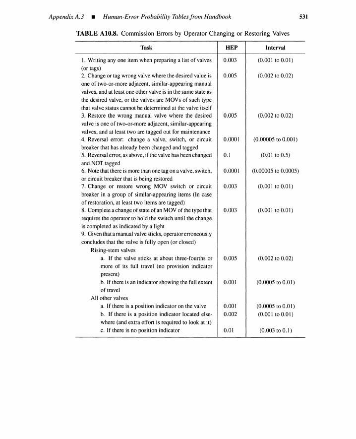
Appendix A.3 • Human-Error Probability Tables from Handbook
TABLE AIO.S. Commission Errors by Operator Changing or Restoring Valves
531
0.005 (0.002 to 0.02)
0.001 (0.0005 to 0.01)
0.001 (0.0005 to 0.01)
0.002 (0.001 to 0.01)
0.01 (0.003 to 0.1)
0.005 (0.002 to 0.02)
0.0001 (0.00005 to 0.001)
0.1 (0.01 to 0.5)
0.0001 (0.00005 to 0.0005)
0.003 (0.001 to 0.01)
0.003 (0.001 to 0.01)
Task
1. Writing anyone item when preparing a list of valves
(or tags)2. Change or tag wrong valve where the desired value is
one of two-or-more adjacent, similar-appearing manual
valves, and at least one other valve is in the same state as
the desired valve, or the valves are MOYs of such type
that valve status cannot be determined at the valve itself3. Restore the wrong manual valve where the desired
valve is one of two-or-more adjacent, similar-appearing
valves, and at least two are tagged out for maintenance4. Reversal error: change a valve, switch, or circuit
breaker that has already been changed and tagged5. Reversal error, as above, if the valve has been changed
and NOT tagged6. Note that there is more than one tag on a valve, switch,
or circuit breaker that is being restored7. Change or restore wrong MOY switch or circuit
breaker in a group of similar-appearing items (In case
of restoration, at least two items are tagged)8. Complete a change of state of an MOY of the type that
requires the operator to hold the switch until the change
is completed as indicated by a light9. Given that a manual valve sticks, operator erroneously
concludes that the valve is fully open (or closed)
Rising-stem valves
a. If the valve sticks at about three-fourths or
more of its full travel (no provision indicator
present)
b. If there is an indicator showing the full extent
of travel
All other valves
a. If there is a position indicator on the valve
b. If there is a position indicator located else-
where (and extra effort is required to look at it)
c. If there is no position indicator
REP
0.003
0.005
Interval
(0.001 to 0.01)
(0.002 to 0.02)
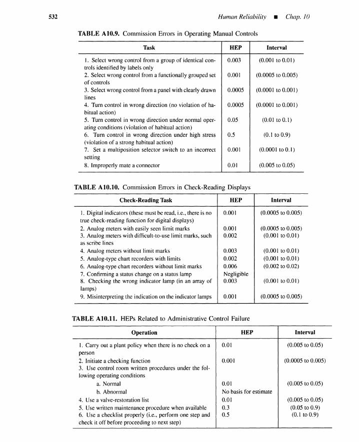
532 Human Reliability _ Chap. 10
TABLE AIO.9. Commission Errors in Operating Manual Controls
Task HEP Interval
I. Select wrong control from a group of identical con- 0.003 (0.001 to 0.01)troIs identified by labels only2. Select wrong control from a functionally grouped set 0.001 (0.0005 to 0.005)of controls
3. Select wrong control from a panel with clearly drawn 0.0005 (0.000 I to 0.00 I)lines4. Turn control in wrong direction (no violation of ha- 0.0005 (0.0001 to 0.001)
bitual action)5. Turn control in wrong direction under normal oper- 0.05 (0.01 to 0.1)
ating conditions (violation of habitual action)6. Turn control in wrong direction under high stress 0.5 (0.1 to 0.9)
(violation of a strong habitual action)7. Set a multi position selector switch to an incorrect 0.001 (0.0001 to 0.1)setting
8. Improperly mate a connector 0.01 (0.005 to 0.05)
TABLE AlO.lO. Commission Errors in Check-Reading Displays
Check-Reading Task
1. Digital indicators (these must be read, i.e., there is notrue check-reading function for digital displays)
2. Analog meters with easily seen limit marks3. Analog meters with difficult-to-use limit marks, suchas scribe lines
4. Analog meters without limit marks
5. Analog-type chart recorders with limits
6. Analog-type chart recorders without limit marks
7. Confirming a status change on a status lamp8. Checking the wrong indicator lamp (in an array oflamps)
9. Misinterpreting the indication on the indicator lamps
HEP
0.001
0.0010.002
0.003
0.002
0.006
Negligible0.003
0.001
Interval
(0.0005 to 0.005)
(0.0005 to 0.005)(0.00 I to 0.0 I)
(0.001 to 0.01)
(0.00 I to 0.0 I)(0.002 to 0.02)
(0.001 to 0.0 I)
(0.0005 to 0.005)
TABLE AIO.ll. HEPs Related to Administrative Control Failure
Operation HEP Interval
I. Carry out a plant policy when there is no check on aperson
2. Initiate a checking function3. Use control room written procedures under the fol-lowing operating conditions
a. Normal
b. Abnormal
4. Use a valve-restoration list
5. Use written maintenance procedure when available6. Use a checklist properly (i.e., perform one step and
check it off before proceeding to next step)
0.01
0.001
0.01
No basis for estimate
0.01
0.30.5
(0.005 to 0.05)
(0.0005 to 0.005)
(0.005 to 0.05)
(0.005 to 0.05)
(0.05 to 0.9)(0.1 to 0.9)

Appendix A.3 • Human-Error Probability Tables from Handbook
TABLE AIO.12. Errors in Recalling Special Oral Instruction Items
Task I REP IItems Not Written Down by Recipient
533
Interval
1. Recall any given item, given the following number ofitems to remember
a. 1 (same as failure to initiate task)
b.2
c.3d. 4
e.52. Recall any item if supervisor checks to see that thetask was done
0.001
0.003
0.01
0.03
0.1Negligible
(0.0005 to 0.005)
(0.00 I to 0.0 I)
(0.005 to 0.05)
(0.0 I to O. 1)
(0.05 to 0.5)
Items Written Down by Recipient
I. Recall any item (exclusive of errors in writing) 0.001 (0.0005 to 0.005)
TABLE AIO.13. Failure to Respond to One RandomlySelected Annunciator
Number ofAnnunciators
12345678910
11-1516-2021-40> 40
HEP
0.00010.00060.0010.0020.0030.0050.0090.020.030.050.100.150.200.25
PROBLEMS
Interval
(0.00005 to 0.00 I)(0.00006 to 0.006)
(0.000 I to 0.01)(0.0002 to 0.02)(0.0003 to 0.03)(0.0005 to 0.05)(0.0009 to 0.09)
(0.002 to 0.2)(0.003 to 0.3)(0.005 to 0.5)(0.01 to 0.999)
(0.015 to 0.999)(0.02 to 0.999)
(0.025 to 0.999)
10.1. What category of human error(s) would you say was (were) typical of the followingscenario:
The safety system for a hydrogeneration reactor had safety interlocks that wouldautomatically shut down the reactor if 1) reactor temperature was high, 2) reactorpressure was high, 3) hydrogen feed rate was high, 4) hydrogen pressure washigh, or 5) hydrogen concentration in the reactor was too high. The reliability ofthe sensors was low, so there was about one unnecessary shutdown every week.The operators were disturbed by this, so they disabled the relays in the safetycircuits by inserting matches in the contacts. One day, the reactor exploded.
10.2. Pictorialize a human being as a computer system.

534 Human Reliability _ Chap. 10
10.3. Enumerate human characteristics during panic.
10.4. List performance-shaping factors.
10.5. Consider a novice operator whose task is to select a valve and turn it off when anappropriate light flashes. Assume that the selection error under optimal stress level is0.005 with a 90% confidence interval of (0.002 to 0.01). Calculate error probabilitiesfor the other three levels of stress.
10.6. Four redundant electromagnets that control a safety system are all calibrated by oneelectrician. The failed-dangerous situationoccurs if all four magnetsare miscalibrated.Construct an HRA event tree, following the procedure leading to Figure 10.8.
10.7. Three identical thermocouple temperature sensors are used to monitor a reaction. Allthree are calibrated by the same worker. Because they activatea two-out-of-threelogicshutdown circuit, a failed-dangerous situation occurs if all three, or two out of three,are miscalibrated. Construct an HRA event tree, following the procedure leading toFigure 10.8.
10.8. (a) Enumerate twelve steps for a THERP procedure.(b) Explain five types of dependency formulae for THERP to calculate a failure prob-
ability of activity B, given failure of preceding activity A.
10.9. The tasks described in a procedure manual for dealing with a temperatureexcursion ina chemical reactor are as follows.Task 1: Monitor reactor pressure and temperature. If the pressure or temperature
continue to rise, initiate tasks 2 and 3.Task 2: Override the electronically operated feed valve and shut the feed valve man-
ually.Task 3: Override the electronically controlled cooling water valve, and open valve
manually. If the cooling water supply has failed, turn on the emergency(water tower) supply.
Task 1 is done in the control room. Tasks 2 and 3 are carried out at separatelocations by different operators who receive instructions by walkie-talkies from thecontrol room. Further details for the tasks are as follows.1.1. Read pressure (P).1.2. Read temperature (T).2.1. Open relay RE-6.2.2. Shut feed valve VA-2 manually.3.1. Verify that cooling water pump P-3 is operating.3.2. Open relay RE-7.3.3. Open cooling water valve VA-3 fully.3.3. Verify cooling water flow to reactor by feeling pipe. If no flow, open emergency
water supply VA-4.(a) Construct an HRA event tree for each operator.(b) Quantify the human errors using appropriate HEPs.
10.10. (a) Give performance-shapingfactors used in the HCR model.(b) Describea formulafor determiningan actual response time from a nominalmedian
response time.(c) Explain an HCR model equation for determining a nonresponse probability.
IIncertaintyQuantification
11.1 INTRODUCTION
11.1.1 Risk-Curve Uncertainty
Uncertainty quantifications should precede final decision making based on PRA-established risk curves of losses and their frequency. Consider a set of points on a particularrisk curve: {(F1, L 1), ... , (Fm, Lm)}, where L i is a loss caused by accident scenario i andF; is the scenario frequency (or probability). There are m points for m scenarios. Theoccurrence likelihood of each scenario is predicted probabilistically by its frequency. Wewill see in this chapter that the risk curve is far from exact because the scenario frequency is arandom variable with significant uncertainty. Risk-curve variability is important because itinfluences the decision maker, and gives reliability analysts a chance to achieve uncertaintyreductions.
A particular scenario i and its initiating event is represented by a path on an eventtree, while basic causes of this scenario are analyzed by fault trees. Thus the frequencies ofthese basic causes (or events) ultimately determine the frequency F; of scenario i. In otherwords, the scenario frequency (or probability) is a function of the basic cause frequencies:
(11.1)
A hardware component failure is a typical basic cause; other causes include humanerrors and external disturbances. The failure frequency Aj of component j is estimated fromgeneric failure data, plant-specific failure data, expert evaluation of component design andfabrication, and so on. This frequency estimate takes on a range of values rather than a singleexact value, and some values are more likely to occur than others. The component-failurefrequency can only be estimated probabilistically, and the frequency itself is a randomvariable. As a consequence, the scenario frequency F; is also a random variable.
535
536 Uncertainty Quantification _ Chap. JJ
11.1.2 Parametric Uncertainty and Modeling Uncertainty
The uncertainty in component-failure frequency is a parametric uncertainty becausethe frequency is a basic variable of the scenario frequency function F;, and because thecomponent-level uncertainty stems from uncertainties in the component-lifetime distri-bution parameters. The parametric uncertainty can be due to factors such as statisticaluncertainty because of finite component test data, or data evaluation uncertainty caused bysubjective interpretations of failure data. The data evaluation uncertainty is greater thanthe statistical uncertainty, which can be obtained using a variety of traditional, theoreticalapproaches.
Unfortunately, parametric uncertainty is not the only cause of the risk-curve vari-ability. The scenario frequency function F; itself may not be realistic because of variousapproximations made during event-tree and fault-tree construction and evaluation, and as-sumptions about types of component-lifetime distributions, and because the scenarios arenot exhaustive, with important initiating events being missed. These three sources of risk-curve variability are modeling uncertainties. Elaborate sensitivity analyses and independentPRAs for the same plant must be performed to evaluate modeling uncertainty, and scenariocompleteness can be facilitated by systematic approaches such as a master logic diagram toenumerate initiating events; however, there is no method for ensuring scenario completeness.
11.1.3 Propagation ofParametric Uncertainty
In this chapter, we describe the transformation of component-level parametric un-certainties to system-level uncertainties. Viable approaches include Monte Carlo methods,analytical moment methods, and discrete probability algebra. The Monte Carlo method iswidely applicable, but it requires a mathematical model for the system and a large amount ofcomputer time to reduce statistical fluctuations due to finite simulation trials. The momentmethod is a deterministic calculation, and requires less computation time, but the system-level output function F; must be approximated to make the calculation feasible. Discreteprobability algebra is efficient for output functions with simple structures, but it requires alarge amount of computer memory for complicated functions with many repeated variables.Before describing these propagation approaches, let us first consider the parametric uncer-tainty from the point of view of statistical confidence intervals, failure data interpretation,and expert opinions.
11.2 PARAMETRIC UNCERTAINTY
11.2. 1 Statistical Uncertainty
Statistical uncertainty can be evaluated by classical probability or Bayesian probabil-ity; both yield component reliability confidence intervals, as described in Chapter 7. Thecomponent-level uncertainty decreases as more failure and success data become available.
Another important aspect of statistical uncertainty is common-cause analysis [1].The multiple Greek letter model described in Chapter 9 treats common-cause analysis ofdependent-component failures. The Greek parameters fJ and yare subject to statisticaluncertainty as is the component overall failure rate. Denote by nj the number of common-cause events involving exactly j component failures. Suppose we observe n1, 2n2, and 3n3component failures, thus the total number of failures is n 1 + 2n2+ 3n3.

Sec. JJ.2 • Parametric Uncertainty 537
Consider a situation where this total number is fixed. For Greek parameters fJ and y,the likelihood of observing n1, 2n2, and 3n3 is a multinomial distribution:
Pr{nl' 2n2, 3n31fJ, y} == (1 - fJ)n1[fJ(1 - y)]2n2[fJy]3n3/const.
== fJ2n2+3n3(I _ fJ)n 1 y3n3( 1 _ y)2n2/const.
where the constant is a normalizing factor for the probability:
(11.2)
(11.3)
const. == [numerator] (11.4)
Assume a uniform a priori probability density for fJ and y.
p{fJ, y} == fJo(1 - fJ)Oyo(I - y)o/const. (11.5)
From the Bayes theorem, we have the multinomial posterior probability density of fJand y,
where constants A, B, C, and Dare
A == 2n2 + 3n3
B == nl
C == 3n3
D == 2n2
( 11.6)
(11. 7)
( 11.8)
(11.9)
(I 1.10)
The modes, means, and variances of the posterior density are summarized in Table 11.1.The variances decrease as the total number ofcomponent failures, n 1+2n2+3n3, increases.The uncertainties in the Greek parameters can be propagated to the system level to reflectbasic-event dependencies by methods to be described shortly.
TABLE 11.1. Mode, Mean, and Variance of Common-Cause ParametersfJ and y
Mode
Mean
Variance
A
A+B
A+l
A + B+2
(A + 1)(B + 1)
(A + B + 2)2(A + B + 3)
C
C+D
C+l
C+D+2
(C+ l)(D+ 1)
(C+ D+2)2(C+ D+3)
11.2.2 Data Evaluation Uncertainty
Component-failure data analysis is not completely objective; there are many subjec-tive factors. Typical data include number of component failures m, number of demands n,and component exposure time interval T. The statistical uncertainty assumes that m, n,and T are given constants. In practice, these data must be derived from plant and test data,which involves subjective interpretation. The resultant uncertainties in m, n, and T have

538 Uncertainty Quantification _ Chap. JJ
significant effects on the parametric uncertainty, especially for highly reliable components;one failure per 100 demands gives a failure frequency significantly different from zerofailures per 100 demands.
11.2.2.1 Numberoffailures. Data classification and counting processes are subjectto uncertainty. To determine the number of failures, we must first identify the component,its failure mode or success criteria, and causes of failure.
Failure mode and success criteria. Component failures are frequently difficult todefine precisely. A small amount of leakage current may be tolerable, but at some higherlevel it can propagate system failure. In some cases plant data yield questionable informationabout component-success or -failure states. Suppose the design criteria state that a standbypump must be able to operate continuously for 24 hours after startup. In the plant, however,the standby pump was used for only two hours before being taken off-line; the two hoursof successful operation do not ensure 24 hours of continuous operation.
Failure causes. Double counting must be avoided. If a failure due to maintenanceerror is included as a basic event in a fault tree, then the maintenance failure should not beincluded as a hardware failure event. Functionally unavailable failures and other cascadefailures are often represented by event and fault trees. A common-cause analysis must focuson residual dependencies.
11.2.2.2 Number ofdemands and exposure time. For a system containing r re-dundant components, one system demand results in r demands on a component level. Theredundancy parameter r is often unavailable, however, especially in generic databases, sowe must estimate the average number of components per system. The number of systemdemands also depends on estimated test frequencies; exposure time T varies according tothe number of tests and test duration.
11.2.3 Expert-Evaluated Uncertainty
In some cases the component-failure frequency is estimated solely by expert judgmentbased on engineering knowledge and experience. This is an extreme case ofdata uncertainty.The IEEE Std-500 [2] is a catalogue of component-failure rates based on expert evaluation.Each expert provided four estimates for each failure rate: low, recommended, high andmaximum; then a consensus value was formed for each category (low, recommended, etc.)by geometric averaging,
[
n ] lin
A= nA;1=1
(11.11 )
where Ai is expert i value, and n is the number of experts (about 200). The a prioridistribution for the failure rate or the component unavailability is then modified by plant-specific data via the Bayes theorem [3]. Human-error rates are estimated similarly.
Apostolakis et al. [4] found that expert opinions were biased toward low failurefrequencies. Mosleh and Apostolakis [3,5] showed that the geometric averaging of expertopinions is based on three debatable assumptions: the experts are independent, they areequally competent, and they have no systematic biases. This aspect is discussed again inSection 11.4.6.
Sec. 11.3 • Plant-Specific Data
11.3 PLANT-SPECIFIC DATA
539
In this section, we describe how to combine expert opinion and generic plant data intoplant-specific data to evaluate component-unavailability uncertainty.
11.3.1 Incorporating Expert Evaluation asa Prior
Suppose that m 1 fuse failures are observed during n1 demands at plant 1. Thisinformation constitutes plant-specific data D1 about the fuse failures. These data must becombined with expert opinions EX.
Denote by Ql the fuse-failure probability at plant 1. Assume a priori probabilitydensity p{ Ql}. This density is derived from expert knowledge EX. From the Bayestheorem, the posterior probability density of the fuse-failure probability Ql, given theplant-specific data D1, becomes
p{QIID1} = Pr{D1IQl}P{Ql}/const.
= Pr{ml,nlIQl}p{Ql}/const.
= p{Ql}Q~l(I - Ql)n\-ml/const.
(11.12)
(11.13)
(11.14)
where the constants are normalizing factors for p{ Q11 D1}. The posterior density representsthe uncertainty in the fuse-failure probability. This uncertainty reflects the plant-specificdata and expert opinion. This is a single-stage Bayesian approach, and is similar to theBayes formula in Chapter 7.
11.3.2 Incorporating Generic Plant Data as aPrior
11.3.2.1 Generic and plant-specific data. Component-failure data from one plantcannot be applied directly to another plant because of differences in design, operatingprocedures, maintenance strategies, or working conditions. Denote by Di, k ~ 2, thesimilar fuse data in other plants. We now combine plant-specific data D1, generic plantdata D2 to DN+1, and expert opinion EX to derive a probability density for the fuse-failureprobability Ql of plant 1.
Consider a total of N + 1 plants. Plant 1 is the plant for which the fuse failureprobability Ql is to be evaluated. Suppose that the experience of generic plant k has beenmk failures out of nk demands. Then the generic data are
k = 2, ... , N + 1 (11.15)
11.3.2.2 Single-stage Bayesformula. A single-stage Bayes formula for combiningthe plant-specific and generic data is
p{QIID1, ••• , DN+1} = Pr{D1, ... , DN+1IQl}P{Ql}/const. (11.16)
In this formula, the likelihood Pr{D1, ... , DN+11 Ql} is the probability of obtaining theplant-specific and generic data when fuse-failure probability Ql is assumed for our plant.However, generic plants have different failure probabilities from Ql and the likelihood ofgeneric plant data cannot be determined, which is the reason for using a two-stage Bayesapproach, where each plant has its own fuse-failure probability.
11.3.2.3 Two-stage Bayesformula
Second-stage Bayesformula. Denote by G = (D2 , ••• , DN+1) the generic plantdata. The Bayes formula (11.14) is rewritten to include generic data D2 , ••• , DN+1 as a
540 Uncertainty Quantification • Chap. 11
condition:
(11.17)
Because the plant-specific data are obtained independentlyof the generic plant data,
(11.18)
Thus
p{ QtlD 1 , G} == PrIm I, nIl QI }p{ QIIG}/const. (11.19)
== p{ QtlG} Q7' 1(1 - QI )n\-m 1/const, (11.20)
The a priori density p{ QIIG} in (11.20) is obtained by the first-stage Bayes formuladescribed in the next section. This approach is called a two-stage Bayes approach becausetwo Bayes equations are used [4]; the first stage yields the a priori density p{ QtlG}, andthe second stage the a posteriori density p{ QII D 1, G} by (11.20).
First-stage Bayesformula. Imagine that fuse-failureprobabilities are N + 1 sam-ples taken at random from a population. We do not know the exact fuse-failure probabilitypopulation, however, and we consider r candidate populations. Denote by ¢ the indicatorvariable of these populations. From expert knowledge EX, we only know a priori thatpopulation 1 is likely with probability Pr{¢ == I}, population 2 with probability Pr{¢ == 2},and so on:
Pr{¢ == j}, j == 1, ... , r, (r ~ 1) (11.21 )
Denote by¢j (Q) the density for population j. In terms of the populations, the a prioridensity is
r
p{ QIIG} == L p{ QII¢ == j, G}Pr{c/J == JIG}j=1
r
== L p{ Qllc/J == j}Pr{c/J == JIG}j=1
(11.22)
(11.23)
Note in (11.22) that QI is sampled from population j independently of generic data G,given population j. Thus
p{ Qllc/J == j, G} == p{ Qllc/Jj == j} (11.24)
Consider the conditional probability density p{ QII¢ == j}. In this expression, thefuse-failure probability QI is a random sample from population j. Because the populationhas unavailability distribution¢j( Q), we have
(11.25)
(11.26)
Thus the a priori density isr
p{QIIG} == L¢j(QI)Pr{¢ == JIG}j=1
This shows that the a priori density is a weighted sum of populations, where probabilityPr{c/J == JIG} is a weighting factor.
Using the Bayes theorem, the weighting factor can be expressed as
Pr{c/J == JIG} == Pr{c/J == j}Pr{GIc/J == j}/const. (11.27)

Sec. 11.4 • Log-Normal Distribution 541
Because the N generic failure probabilities are sampled at random from given populationj, we obtain
where
N+I
Pr{GI¢ == j} == nPr{mk, nkl¢ == j}k=2
(11.28)
Pr{mk>nkl¢ = j} = Jd ¢j(Qk)(~:)Q~k(1- Qk)nk-mkdQk. (11.29)k == 2, ... , N + 1
Two-stage Bayes approach. The two-stage Bayes approach proceeds as follows(see Problem 11.2 for populations of discrete Q values).
1. The likelihood of generic plant data Di, given population j, is obtained from(11.29).
2. The likelihood of N generic plants data G, given population j, is obtained fromthe product expression (11.28).
3. The a priori probability of population j is given by Pr{¢ == j}, which is basedon expert knowledge EX. This distribution is modified by the first-stage Bayesformula (11.27) to reflect the generic data for N plants.
4. The new a priori density p{ QIIG} is obtained by the weighted sum (11.26).
5. The a posteriori probability density is evaluated using the second-stage Bayesformula (11.14).
11.4 LOG-NORMAL DISTRIBUTION
11.4.1 Introduction
The log-normal distribution plays an important role in uncertainty propagation be-cause reliability parameter confidence intervals such as unavailability and failure rates areoften expressed by multiplicative error factors, an AND gate output becomes a log-normalrandom variable when input variables are log-normal, and log-normal random variables canbe used to represent multiplicative dependencies among experts or components. Unfortu-nately, the OR gate output is not a log-normal variable even if input variables are log-normal.This section describes the log-normal distribution, its relation to confidence intervals, ANDgate output characteristics, and a multiplicative dependency model.
11.4.2 Distribution Characteristics
Because a random variable can be viewed as having a range of values, a probabilitydistribution, such as the log-normal, can be assigned this range to obtain the likelihood ofoccurrence of anyone particular value.
When the range or the confidence interval of a variable is expressed as a multiplicativerather than additive error factor, the log-normal is the proper distribution to describe thevariable.
Variable Q has a log-normal distribution if its natural logarithm X == In Q has anormal distribution with mean Jvt and variance a 2• Characteristics of this distribution aresummarized in Table 11.2. The density function is shown in Figure 11.1. Because parameter
542 Uncertainty Quantification _ Chap. JJ
j1., is the median of In Q, the median Qof Q is
Q== exptu.) (11.30)
The mode, mean, and variance can be calculated from the median. The mode is smallerthan the median, while the mean Q is larger than the median; these differences becomemore significant as parameter a 2 becomes larger:
Mode == Qexp(-a 2) < Median == Q< Mean == Q == Qexp(0.5a 2
) (11.31)
The variance is
(11.32)
TABLE 11.2. Log-Normal Distribution
Symbol
Variable
Location Parameter
Scale Parameter
Density
1 - 2a Error Factor
1 - 2a Interval
Median QParameter jl
a point L
Parametera
Median QMode
MeanQ
Variance V {Q}
Q.\.= Ql···Q"QsQs
V{Qs)
11.4.3 Log-Normal Determination
log -gau*(jl, a 2)
0< Q
-00 < jl < 00
O<a
_1_, exp [_1. (In Q-J-t)2]Jii(JQ 2 (J
K
[QL == Q/K, Qu == QK]JQUQL
InQ
Prix ~ L) = a, x ~ gau*(O, 1)
(In K)/ L
expuz.)
Qexp(-a 2)
Qexp(O.5a2)
(Q)2[(Q/Q)2 - 1]
Suppose that a random variable Q has a 1 - 2a confidence interval between QL ==QfK and Qu == QK, where Qis the median and K is a multiplicative error factor constantgreater than one. In other words, let Q Land Qu be the 1 - a and a points, respectively.*
Pr{Q:::: QLl == I-a, Pr{Q 2: Qul == a (11.33)
*QL and Qu are also called IOOath and 100(1 - a)th percentiles, respectively.
Pr{ Q ::: QL} == a, Pr{ Q ::: Qu} == I - a
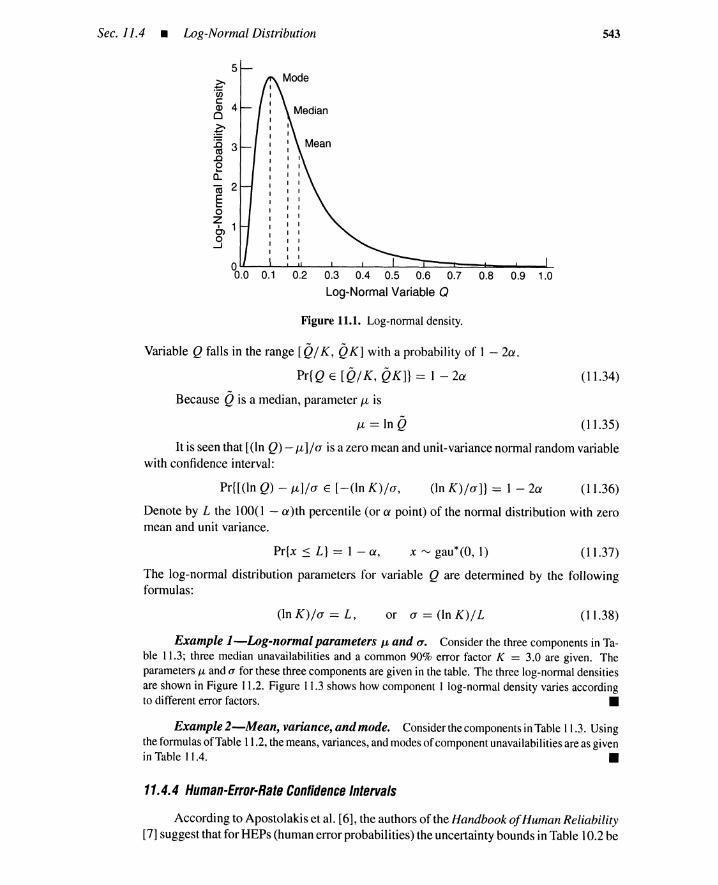
Sec. J1.4 • Log-Normal Distribution
5
~·wai 4o~:0 3as.0oet(ij 2E'-o~10)o
.....J
0.1 0.2 0.3 0.4 0.5 0.6 0.7 0.8 0.9 1.0
Log-Normal Variable Q
Figure 11.1. Log-normal density.
Variable Q falls in the range [Q/ K, QK] with a probability of I - 2a.
Pr{Q E [Q/ K, QK]} == 1 - 2a
Because Qis a median, parameter JvL is
J-l == InQ
543
(11.34)
(11.35)
It is seen that [(In Q) - JvL]/a is a zero mean and unit-variance normal random variablewith confidence interval:
Pr{[(ln Q) - JvL]/a E [-(In Kv]«, (In K) / a]} == 1 - 2a (11.36)
Denote by L the 100(1 - a)th percentile (or a point) of the normal distribution with zeromean and unit variance.
Pr{x:s L} = I-a, x '" gau*(0, I) (11.37)
The log-normal distribution parameters for variable Q are determined by the followingformulas:
(In K)/a == L, or a == (In K) / L (11.38)
Example l-s-Log-normal parameters J..t and 0'. Consider the three components in Ta-ble 11.3; three median unavailabilities and a common 90% error factor K = 3.0 are given. TheparametersJJ; and a for these threecomponentsare givenin the table. The three log-normal densitiesare shownin Figure I1.2. Figure I 1.3shows how component I log-normal density variesaccordingto differenterror factors. •
Example 2-Mean, variance, and mode. ConsiderthecomponentsinTable11.3. Usingtheformulas ofTable11.2,themeans,variances, andmodesofcomponentunavailabilities areasgivenin Table 11.4. •
11.4.4 Human-Error-Rate Confidence Intervals
According to Apostolakis et al. [6], the authors of the Handbook ofHuman Reliability[7] suggest that for REPs (human error probabilities) the uncertainty bounds in Table 10.2 be

544 Uncertainty Quantification • Chap. 11
80
70
~·Cii 60c:Q)
0
~50
:0co
40.00~
a..eo 30E~
0Z 200,0
--J10
0.02 0.04 0.06 0.08 0.10 0.12 0.14 0.16 0.18 0.20
Unavailability Q
Figure 11.2. Log-normal densities for the three components.
80
Median = 0.074170
~.~ 60Q)
c~ 50:0~ 40ea..
30EQ)
§ 20a.E8 10
K=3.0
O~----...&...--_~~...L.-----a..----~~---------,------,--~
0.00 0.02 0.04 0.06 0.08 0.10 0.12 0.14 0.16 0.18 0.20
Unavailability Q
Figure 11.3. Component 1 log-normal density with differenterror factors.
used as the 0.95 and 0.05 points (i.e., 5th and 95th percentiles) of a log-normal distribution.Others use these bounds as 0.9 and 0.1 points because experts tend to be overconfident intheir assessment of HEP distributions. Swain and Guttmann do not appear to object to thispractice.
For HEPs greater or equal to 0.1, reference [8] recommends a beta density to describeHEP uncertainty.
Pr{Q ~ HEP < Q + d Q} == _I- Qr(1 - Q)'\'d Q, 0 :s Q :s I (11.39)const.
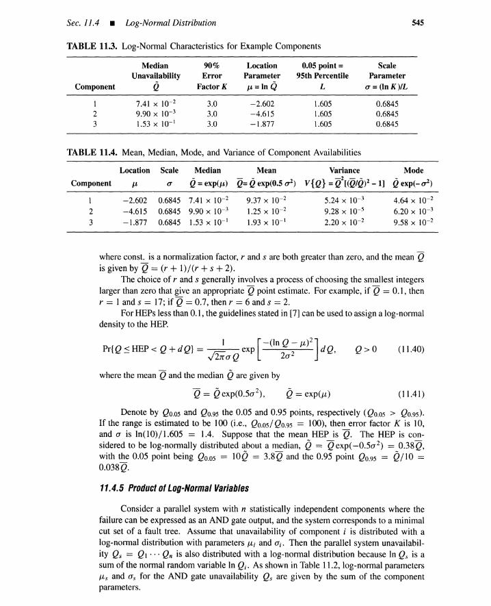
Sec. 11.4 • Log-Normal Distribution
TABLE 11.3. Log-Normal Characteristics for Example Components
Median 90% Location 0.05 point = ScaleUnavailability Error Parameter 95th Percentile Parameter
Component Q Factor K p,=ln Q L 0' = (In K)/L
I 7.41 x 10⁻² 3.0 -2.602 1.605 0.68452 9.90 x 10⁻³ 3.0 -4.615 1.605 0.68453 1.53 x 10- 1 3.0 -1.877 1.605 0.6845
TABLE 11.4. Mean, Median, Mode, and Variance of Component Availabilities
545
Location Scale Median Mean Variance Mode
Q= exp(p,) Q= Qexp(0.5 0'2)-2 - - Qexp(-0'2)Component p, 0' V {Q} = Q [(Q/Q)2 - 1]
1 -2.602 0.6845 7.41 x 10⁻² 9.37 X 10⁻² 5.24 X 10⁻³ 4.64 X 10⁻²
2 -4.615 0.6845 9.90 x 10⁻³ 1.25 X 10⁻² 9.28 X 10⁻⁵ 6.20 X 10⁻³
3 -1.877 0.6845 1.53 x 10- 1 1.93 X 10- 1 2.20 X 10⁻² 9.58 X 10⁻²
where const. is a normalization factor, rand s are both greater than zero, and the mean Qis given by Q == (r + l)/(r + s + 2).
The choice of rand s generally involves a process of choosing the smallest integerslarger than zero that give an appropriate Q point estimate. For example, if Q == 0.1, thenr == 1 ands == 17; if Q == 0.7, then r == 6 ands == 2.
For HEPs less than 0.1, the guidelines stated in [7] can be used to assign a log-normaldensity to the HEP.
I [-on Q - ~)2]Pr{Q:sHEP< Q+dQ} == r;c exp 2 dQ,
v2rraQ 2a
where the mean Qand the median Qare given by
Q>O (11.40)
-,.., 2Q == Q exp(0.5a ), Q== exp(~) (11.41 )
Denote by QO.05 and QO.95 the 0.05 and 0.95 points, respectively (QO.05 > QO.95).If the range is estimated to be 100 (i.e., QO.05/ QO.95 == 100), then error factor K is 10,and a is In(10) /1.605 == 1.4. Suppose that the mean HEP is Q. The HEP is con-sidered to be log-normally distributed about a median, Q == Qexp(-O.5a2) == 0.38Q,with the 0.05 point being QO.05 == 10Q == 3.8Q and the 0.95 point QO.95 == Q/IO ==0.038Q.
11.4.5 Product ofLog-Normal Variables
Consider a parallel system with n statistically independent components where thefailure can be expressed as an AND gate output, and the system corresponds to a minimalcut set of a fault tree. Assume that unavailability of component i is distributed with alog-normal distribution with parameters u, and a.. Then the parallel system unavailabil-ity Qs == QI··· Qn is also distributed with a log-normal distribution because In Qs is asum of the normal random variable In Qi. As shown in Table 11.2, log-normal parameters~s and as for the AND gate unavailability Qs are given by the sum of the componentparameters.
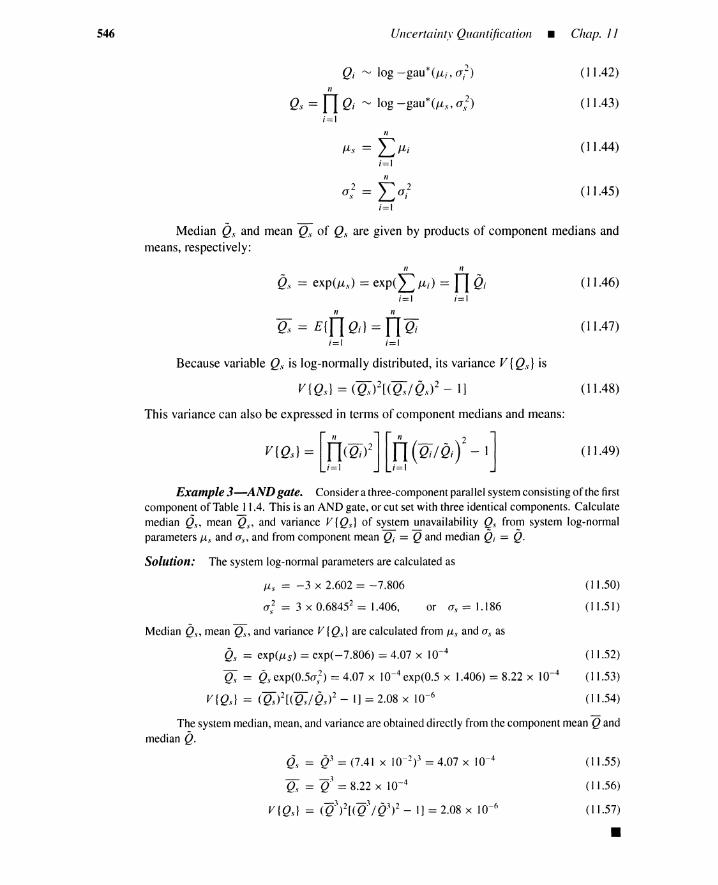
546 Uncertainty Quantification • Chap. JJ
n
Qs == nQ; ~ log -gau*(Jls, a});=)
n
u., == L Jl;;=)
n
a} == Lal;=)
( 11.42)
( 11.43)
(I 1.44)
(I 1.45)
Median o. and mean Q.\. of Qs are given by products of component medians andmeans, respectively:
n n
Qs == exp(Jls) == expeL Jl;) == nQ;;=1 ;=1
n n
Q.\. == Efn Q;} == Il Q;;=1 ;=1
Because variable Q, is log-normally distributed, its variance V fQs} is
This variancecan also be expressed in terms of component medians and means:
(I 1.46)
(I 1.47)
(11.48)
(I 1.49)
Example 3-ANDgate. Consider a three-component parallel system consisting of the firstcomponent of Table 11.4. This is an AND gate, or cut set with three identical components. Calculatemedian a: mean Q.P and variance V IQ.\.} of system unavailability Qs from system log-normalparameters Ils and a., and from component mean Q; = Q and median Q; = Q.
Solution: The system log-normal parameters are calculated as
u, = -3 x 2.602 = -7.806
a} = 3 x 0.68452 = 1.406, or as = 1.186
Median o: mean Q.n and variance V IQs} are calculated from J1s and a, as
Q.\. = exp(J1s) = exp(- 7.806) = 4.07 x 10⁻⁴
Q.\. = Q.\. exp(0.5a}) = 4.07 x 10- 4 exp(0.5 x 1.406) = 8.22 x 10- 4
VIQs} = (Q.\.)2[(Qs/Qs)2 - I] = 2.08 X 10⁻⁶
( 11.50)
(11.51 )
( 11.52)
( 11.53)
(11.54)
The system median, mean, and variance are obtained directly from the component mean Q andmedian Q.
Qs = Q3 = (7.41 X 10⁻²) 3 = 4.07 X 10- 4
- -3 -4Q.\. = Q = 8.22 x 10
VIQs} = (Q3)2[(Q3/ Q3)2 - I] = 2.08 X 10⁻⁶
( 11.55)
( 11.56)
( 11.57)
•
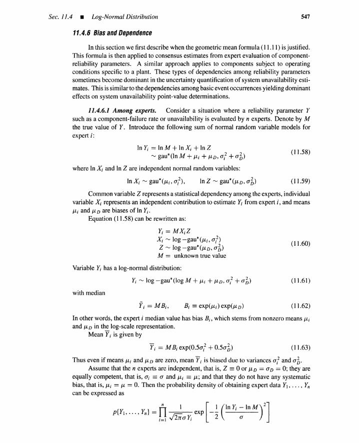
Sec. 11.4 • Log-Normal Distribution
11.4.6 Bias and Dependence
547
In this section we first describe when the geometric' mean formula (11.11) is justified.This formula is then applied to consensus estimates from expert evaluation of component-reliability parameters. A similar approach applies to components subject to operatingconditions specific to a plant. These types of dependencies among reliability parameterssometimes become dominant in the uncertainty quantification of system unavailability esti-mates. This is similar to the dependencies among basic event occurrences yielding dominanteffects on system unavailability point-value determinations.
11.4.6.1 Among experts. Consider a situation where a reliability parameter Ysuch as a component-failure rate or unavailability is evaluated by n experts. Denote by Mthe true value of Y. Introduce the following sum of normal random variable models forexpert i:
In Yi == In M + In Xi + In Zrv gau*(ln M + IJ-i + IJ-D, al + ab)
where In Xi and In Z are independent normal random variables:
(11.58)
In Xi rv gau*(IJ-i,a?), (11.59)
(11.60)
Common variable Z represents a statistical dependency among the experts, individualvariable Xi represents an independent contribution to estimate Yi from expert i, and meansIJ-i and IJ- D are biases of In Yi.
Equation (11.58) can be rewritten as:
Yi == MXiZXi rv log -gau*(IJ-i, al)Z rv log -gau*(IJ-D' ab)
M == unknown true value
Variable Yi has a log-normal distribution:
Yi rv log -gau*(1og M + IJ-i + IJ-D, al + a~)
with median
(11.61)
Yi == MB i , B, == exp(IJ-i)exp(IJ-D) (11.62)
In other words, the expert i median value has bias Bi, which stems from nonzero means IJ-iand IJ- D in the log-scale representation.
Mean f i is given by
- 2 2Y i == M B, exp(0.5ai + 0.5a D) (1 1.63)
Thus even if means IJ-i and IJ-D are zero, mean Vi is biased due to variances al and aboAssume that the n experts are independent, that is, Z == 0 or IJ- D == aD == 0; they are
equally competent, that is, a, == a and IJ-i == IJ-; and that they do not have any systematicbias, that is, IJ-i == IJ- == O. Then the probability density of obtaining expert data Y1, ••• , Yn
can be expressed as
n 1 [I (InYi-InM)2]p{Y i , ••• , Yn ) =nv'2ii exp--i=l Lno Yi 2 a

548 Uncertainty Quantification • Chap. JJ
Maximizing this density with respect to M gives the maximum-likelihood estimator of theunknown true value:
[
n ] Jln
M== nf;;=1
(11.64)
Thus under the dubious assumptions above, the geometric mean (11.11) is the best estimateof component-failure rate or unavailability. The maximum-likelihood estimator can begeneralized to cases where the three assumptions do not hold.
11.4.6.2 Amongcomponents. Ifexpert i is replaced by componenti in the model of(11.60), it applies to the case where unavailabilities of n components have biases and statis-tical dependencies [9]. Such biases and dependencies represent, for instance, plant-specificoperating conditions such as chemical corrosion. The resultant component-reliability pa-rameter dependencies propagate to system levels by the methods described in the nextsection.
Example 4-Bias due to management deficiency. Assume the cooling system in Fig-ure 11.4 with a principal pump that normally sends cooling water to a designated location [10]. Astandby emergency pump sends water when the principal pump is down. A normally closed valvelocated upstream of the emergencypump must be opened on demand when the emergencypump isneeded. The principal pump and emergency pump are of different type and manufacture. All threecomponents are maintained by the same crew, however, and failure rates are affected by the qualityof the maintenance team. This quality of maintenance, which is affected by plant organizationandmanagementpolicies, will influenceall three componentsand raises or lowers their failure rate.
PrincipalPump
Figure 11.4. A cooling system with prin-cipal and standby pumps.
StandbyPump
The event that there is no cooling water output X is
X = XIX2 V XIX)
where Xl = the principal pump fails to delivercooling water;X2 = the emergencypump fails to delivercooling water;X) = the valve fails to open on demand.
The failure probabilityof the cooling system is, therefore
If the threeeventsare independentwith the same failureprobability0.1, then the cooling system failsabout lin 50 demands.
P{Xl = 0.1 x 0.1 + 0.1 x 0.1 - 0.1 x 0.1 x 0.1 = 0.019

Sec. 11.5 • Uncertainty Propagation 549
Assume that the maintenance quality is so low that the principal pump fails with probability0.2, and that the emergency pump and the valve fail with probability 0.8. These failures still occur in-dependently, but failure probabilities have increased. The cooling-system failure probability becomesmuch larger (about one in five demands) than in the former case:
PIX} = 0.2 x 0.8 + 0.2 x 0.8 - 0.2 x 0.8 x 0.8 = 0.192
The high failure probability, 0.8, of the standby components may be due to latent failures prior to theprincipal pump failure. •
11.5 UNCERTAINTY PROPAGATION
To facilitate the quantitative analysis of fault trees, it is convenient to represent fault trees inmathematical form: the structure functions and minimal cut set representations describedin Chapter 8 are appropriate tools for this purpose. System unavailability Qs(t) may beobtained by methods such as complete expansion and partial pivotal decomposition of thestructure function. For large and complex fault trees, the inclusion-exclusion principlebased on minimal cut sets can be used to approximate Qs(t).
Figure 11.5 has the following structure function 1/1 and the corresponding systemunavailability Qs(t).
1/I(Y) = 1 - (1 - Y1)(1 - Y2Y3)
Qs = 1 - (1 - Ql)(l - Q2Q3)
(11.65)
(11.66)
The inclusion and exclusion principle or an expansion of (11.66) gives the exact unavail-ability
Qs = QI + Q2Q3 - QI Q2Q3
which is approximated by the first bracket
Qs = QI + Q2Q3
(11.67)
(11.68)
Figure 11.5. Reliability block diagram and fault tree for example problem.
For independent basic events, system unavailability Qs is a multiple-linear polynomialfunction of component unavailabilities QI, ... , Qn.
(11.69)
550 Uncertainty Quantification • Chap. JJ
where each term in the sum is a product of j component unavailabilities. For the systemunavailabilityexpression (11.67),
Qs == QI + Q2Q3 - QI Q2Q3'-y-I '-v-' '-v-"j=1 j=2 j=3
(11.70)
(11.71)
(11.72)
(11.73)
For dependent basic events, consider a 2/3 valve system subject to a common cause.As shown in Chapter 9, the demand-failure probability V of the system is
V ::;: V3 + 3V2 + 3VI2
~ V3 + 3V2 == Y~A + 3(1/2)(1 - Y)~A
== Y == F(A,~, Y)
where A is an overall failure rate, and fJ and yare multiple Greek letter parameters. TheA, ~, and y uncertainties must be propagated to fault-tree top-event levels through themultiple-linear function F.
As shown in Sections 11.7.5and 11.7.6, the multiple-linearity simplifies the unavail-ability-uncertainty propagation. Unfortunately, the output function Y == F(X1, ••• , Xn ) inthe uncertainty propagation is not necessarily multiple-linear, especially when some basicevents have statistically dependent uncertainties. Consider valve failures to be independentin (I 1.71): V == 3V1
2• If the valve unavailability uncertainties are completely depen-dent, the uncertainty of V? must be evaluated from the uncertainty of VI.
When fixed values are used for the failure rates and other parameters, the systemunavailability is a point value. Because of the uncertainties and variations in the failurerates and parameters, however, these quantities are treated as random variables and, be-cause the system unavailability Qs(t) is a function of these random variables, it is itself arandom variable. The term uncertainty propagation refers to the process of determining theoutput variable distribution in terms of the basic variable distributions, given a functionalrelation Y == F(X1 , ••• , Xn ) . Three uncertainty propagation approaches are the MonteCarlo method, the analytical moment method, and discrete probability algebra: These aredescribed in the next three sections.
11.6 MONTE CARLO PROPAGATION
11.6. 1 Unavailability
Uncertainty propagation is conveniently done by a computerized Monte Carlo tech-nique. In its simplest version, component unavailabilities are sampled from probabilitydistributions, these unavailabilities are then propagated toward a top event, and a pointvalue is calculated for system unavailability. The Monte Carlo sampling is repeated alarge number of times, and the resultant point values are then used to evaluate the systemunavailability uncertainty,
The SAMPLE computer program uses Monte Carlo to obtain the mean, standarddeviation, probability range, and distribution for a function Y == F(X1, ••• , Xn ) [11]. Thisfunction can, for example, be system unavailability Qs in terms of component unavailabil-ities QI, ... , Qn. The function F could also be system reliability R.." in terms of variablecomponent-failure and -repair rates. Common-cause parameters such as those in (11.72)may be included as basic variables. Multiplicativedependency models such as (11.60) canalso be simulated by Monte Carlo.

Sec. 11.6 • Monte Carlo Propagation 551
Given a function Y = F(X1, ••• , Xn ) , values of the distribution parameters of theindependent variables, and a specific input distribution, SAMPLE obtains a Monte Carlosampling Xl, ••• ,Xn from the input variable distributions and evaluates the correspondingY = F(XI' ... ,xn ) . The sampling is repeated N (input parameter) times, and the resultantestimates of Yare ordered in ascending values YI ~ Y2 ~ ... ~ YN to obtain the percentilesof the Y distribution. The program has a choice of failure distributions as an input option(normal, log-normal, log-uniform, etc.).
Example 5-SAMPLE program. To illustrate the SAMPLE program and propagationtechnique we consider the system for which a reliability block diagram and fault tree are shown inFigure 11.5. The event data that contain the uncertainties in the above system are given in Table 11.3.
The system unavailability Qscan be approximated as the first bracket of the inclusion-exclusionformula:
(11.74)
This function is included in the SAMPLE input as a function supplied by the user. The results of thecomputations are given in terms of probability confidence limits; the output is shown in Table 11.5.
TABLE 11.5. SAMPLE output
Distribution Confidence Limits
Confidence (%)
0.51.02.05.0
10.020.025.030.040.050.060.070.075.080.090.095.097.599.099.5
Function Value
1.77 X 10- 2
1.88 X 10- 2
2.21 X 10- 2
2.66 X 10- 2
3.34 X 10- 2
4.47 X 10- 2
5.11 X 10- 2
5.69 X 10- 2
6.65 X 10- 2
7.67 X 10- 2
9.23 X 10- 2
1.09 X 10- 1
1.19 X 10- 1
1.31 X 10- 1
1.77 X 10- 1
2.22 X 10- 1
2.56 X 10- 1
3.15 X 10- 1
3.91 X 10- 1
Sample size: 1200Mean: 9.48 x 10- 2
Variance: 4.53 x 10- 3
Standard deviation: 6.73 x 10- 2
Function values are the upper bounds of the indicated confidence limits. The 50% value is themedian of the distribution, and the 95th and 5th percentiles are the upper and lower bounds of the90% probability interval, respectively. •
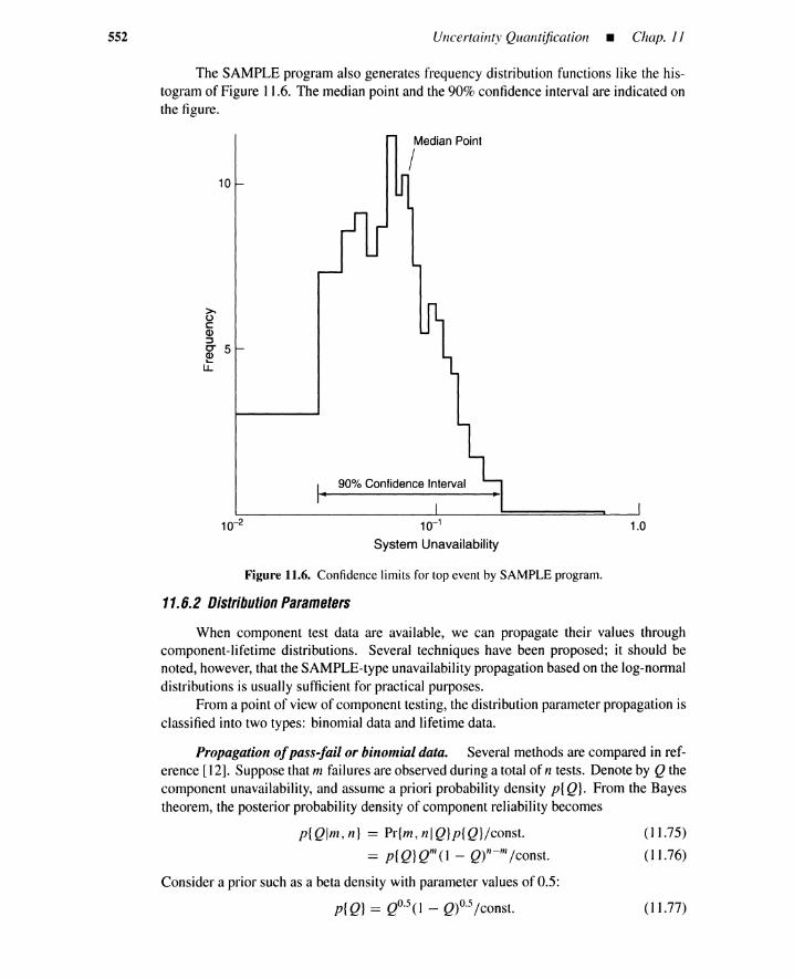
552 Uncertainty Quantification _ Chap. JJ
The SAMPLE program also generates frequency distribution functions like the his-togram of Figure 11.6. The median point and the 90% confidence intervalare indicated onthe figure.
10
Median Point
I
~ocQ)::Jg 5L..
U.
\-
10-1
System Unavailability
Figure 11.6. Confidence limits for top event by SAMPLE program.
11.6.2 Distribution Parameters
1.0
When component test data are available, we can propagate their values throughcomponent-lifetime distributions. Several techniques have been proposed; it should benoted, however, that the SAMPLE-type unavailability propagationbased on the log-normaldistributions is usually sufficientfor practical purposes.
From a point of view of component testing, the distribution parameter propagation isclassified into two types: binomial data and lifetime data.
Propagation ofpass-fail or binomial data. Several methods are compared in ref-erence [12]. Suppose that m failures are observedduring a total of n tests. Denote by Q thecomponent unavailability, and assume a priori probability density p{ Q}. From the Bayestheorem, the posterior probability density of component reliability becomes
p{Qlm, n} == Pr{m, nIQ}p{Q}/const.
== p{Q}Qm(1 _ Q)"-m/const.
Consider a prior such as a beta density with parameter values of 0.5:
p{ Q} == QO.5 (I - Q)O.5/const.
(11.75)
(11.76)
(11.77)

Sec. 11.6 • Monte Carlo Propagation 553
This type of prior is one that contributes little prior information to the analysis relative tothe binomial component test data. The component reliability is sampled from the posteriorbeta distribution with parameters m + 0.5 and n - m + 0.5. This technique is a Bayesmethod.
In a so-called bootstrap method [13], the component unavailability is first estimatedfrom the binomial test data as Q == min. Then the number of failures m" is sampled byMonte Carlo from the binomial distribution o: (1 - Q)n-m. The unavailability estimateQ* == m"In is used as a component unavailability sample.
Propagation oflifetimedata. Maximum-likelihood parameter estimations are sum-marized in Appendix A.I. This estimation starts with censored lifetime data that apply totime-terminated tests and failure-terminated tests. Equation (A.9) shows that a parameterestimator vector is asymptotically distributed and has a multidimension normal distribu-tion. Furthermore, the component unavailability estimator, as shown in (A. 11), is alsoasymptotically distributed with a normal distribution.
Parameter vector sampling from a multidimension normal distribution is called abivariate s-normal technique, while reliability sampling from a single-dimension normaldistribution is a univariate s-normal technique [14]. In the univariate beta technique, thenormal distribution is replaced by a beta distribution; the beta distribution is used because,for values of unavailability smaller than 0.1, the component unavailability distribution isskewed; in addition, under the s-normal assumption, with the unavailability close to zero,a high percentage of the simulated reliability values are smaller than zero.
In the double Monte Carlo technique, a maximum-likelihood estimator (MLE) iJ ofunknown parameter vector () is first calculated from actual data. Artificial lifetime data are
sampled randomly from the distribution determined bye. Another MLE is calculated from
the simulation data, and used as a sample from the distribution parameter e. This is anextension of the bootstrap method for binomial test data.
11.6.3 Latin Hypercube Sampling
The direct Monte Carlo sampling is performed randomly and independently. Thusfor a small sample size, there is a possibility that some regions of variable Xi are neversampled. This results in a large error, especially when there is a lack of sampling forvariables that dominate output Y. The Latin hypercube sampling [IS] is a mixture ofrandom and systematic sampling to ensure that each interval or stratum of variable Xi isvisited by exactly one Monte Carlo sample.
The range of variable Xi is divided into N strata of equal probability liN. A value ofXi is sampled from each stratum according to a probability density proportional to p{Xi},that is, the conditional probability of variable Xi, given that the variable takes on a value inthe stratum. Denote by Xi}, j == 1, ... , N the set of samples of variable Xi; Xi I sampledfrom the first stratum, and X i N from the last stratum. Similar samples are generated forother variables. In a matrix form, we have the following input variable samples.
stratum 1 stratum N
Xll X 1N for variable Xl
X21 X2N for variable X2 (I 1.78)
X n1 X n N for variable X n
554 Uncertainty Quantification _ Chap. JJ
When these samplesare randomly combined, we haveordinaryMonte Carlo samplesfor n-dimension vector (Xl, X2, ••• , X,,). In Latin hypercube sampling, row elements ofthe sampling matrix are randomly permuted within each row; this permutation is repeatedindependently for every row, and a new sampling matrix is obtained. Each column vectorof the resultant sampling matrix becomes an n-dimension Latin hypercube sample. Thuswe havea total of N samples. A value is sampled from each stratum, and this valueappearsexactly once in a column vector sample.
Denote by (Xl, ••• , Xn ) a sample obtained by Latin hypercubesampling. This sampleis distributed according to the original probability density:
(11.79)
Thus component values within a sample vector are independent. Different sample vectorsare not independent any more, however, because a stratum component value appears onlyonce in exactly one Latin hypercube sample.
Example 6-wtin hypercubesampling. Assumethe following samplingdata (N = 3and n = 2):
(-5 1 25)-10 5 20 '
Random permutations in each row may yield
(2~ ~5
(2 dimension,3 strata)
25 )-10
(11.80)
(11.81)
The two-dimension Latin hypercube samples become
( do ), ( ~5 ), ( ~~0 ) (11.82)
•
(11.83)
(11.84)
One advantage of Latin hypercube sampling appears when output Y is dominated byonly a few input variables. The method ensures that each variable is represented in a fullystratified manner, no matter which component turns out to be important [15].
Consider a class of Monte Carlo estimators of the formN
T (YI , ... , YN) = (1/N) L g(Yi )
;=1
where Y; is an output value from Monte Carlo trial i. If g(Y) = Y then T represents thesample mean used to estimate E{Y}. If g(Y) = yk we obtain the kth sample moment. Byletting g(Y) = 1 for Y :::: y, and 0 otherwise, we obtain the usual empirical distributionfunction at point y. Denote by TD and TL estimators of direct Monte Carlo and Latinhypercube sampling, respectively.
The estimator takes different values when Monte Carlo trials of size N are repeated.The estimator variance is
V {T} = N-2 (t V {g(Yi ) } +~ Cov{g(Yi ) , g(yj ) })
The covariance terms are zero for the direct Monte Carlo because the N trials are mutuallyindependent. The twoMonteCarlo methodsyield thesamevarianceterms V {g( Yi ) } becausebasic variable samples in each trial i follow the same distribution. For the Latin hypercube
Sec. JJ.7 • Analytical Moment Propagation 555
sampling, the covariance terms are nonpositive if Y F(X1, ••• ,Xn ) is monotonic ineach of its arguments, and g(Y) is a monotonic function of Y. Thus under the monotonicassumption, the estimator variance V {TL} is no greater than estimator variance V {TD} [15].
11.7 ANALYTICAL MOMENT PROPAGATION
For an AND or OR gate output with independent inputs, mean and variance can be calculatedanalytically from the first and second input moments. As a consequence, fault-tree top-event probability mean and variance can be calculated recursively unless the tree has norepeated basic events. This type of moment propagation is described first.
For fault trees with repeated events, top-event unavailability expressions must beapproximated to make the moment propagation feasible. Typical approximations includefirst bracket inclusion-exclusion, Taylor series expansion, orthogonal expansion, responsesurface methods, analysis of variance, and regression analysis. This section describes thefirst three approximations. References [16-18] describe the remaining three approximationmethods.
11.7.1 AND gate
Equation (11.49) is a special case of variance propagation when component unavail-abilities are log-normally distributed. We consider here how the mean and variance propa-gate through an AND gate with n input components having general distributions.
The top-event unavailability Qs can be expressed as
The mean is
n
Qs == 0 Qi == QI 1\ ... 1\ Qn;=1
n
Qs == 0 Qi;=1
(11.85)
(11.86)
Denote by an overbar an expected value operation. From the definition of variance,
V { Q1 1\ ... /\ Qn} == Q; - (Q s )2
For identical input components,
n n
0 _2 0-2== Q; - (Q;);=1 ;=1
(11.87)
(11.88)
The first and second moments of Qi are sufficient for calculating mean and variancepropagation through an AND gate. These moments, on the component level, are listed inTable 11.6 for the log-normal components in Table 11.4.
Example 7-AND gate exact-momentpropagation. Consider an AND gate with threeidentical components to which the data in the first row of Table 11.6 apply. The variance of the outputevent is
yielding the same result as (11.57) except for round-off errors.
( 11.89)
•

556 Uncertainty Quantification • Chap. JJ
TABLE 11.6. First and Second Moments for Example Components
Component
123
9.37 X 10⁻²
1.25 X 10⁻²
1.93 X 10- 1
V{Q}
5.24 X 10⁻³
9.28 X 10⁻⁵
2.20 X 10⁻²
1.40 X 10⁻²
2.49 X 10⁻⁴
5.93 X 10⁻²
A= l-Q
9.063 X 10- 1
9.875 X 10- 1
8.070 X 10- 1
8.266 X 10- 1
9.752 X 10- 1
6.732 X 10- 1
11.7.2 OR gate
OR gate outputs are not log-normal random variableseven if input variablesare log-normally distributed. However, the firstand second moments propagate in a similar way asfor an AND gate. The exact-moment propagation formulas for the AND and OR gates aresummarized in Table 11.7 together with formulas derived in Section 11.7.6.
TABLE 11.7. Exact and Approximate Moment Propagations for AND and OR
Exact
Approximate
AND GateV{Qt/\···/\Qn}
/I /InQ; - n<Q;)2;=1 ;=1
t(UQir V(QJ
+f.; (IJj Qk)2V(QiIV(QiJ
OR GateV{QtV •..VQn}
/I IInA; - n<A;)2;=1 ;=1
t (U Ajr VIA;)
+f.; (IJ/kr V(A;}V(Ajl
Consideran ORgate withn inputcomponents. Denoteby Ai == I - Qi the availabilityof component i. The top-event unavailability is
n
Qs == I - As == I - nAi == Q. v ... v Qni=1
The mean of Qs is given by
n
Qs == 1-nA;;=1
The variance of Qs is equal to the varianceof As:
11
A"i == nAi == AI /\ ... /\ An;=1
yielding a variance forrnula that is dual with respect to (11.87).
11 nn2 n-2V{QI v··· V Qn} == V{A 1 /\ ••• /\ An} == Ai - (Ai);=1 ;=1
(11.90)
(11.91 )
(11.92)
(11.93)

Sec. 11.7 • Analytical Moment Propagation
For identical input components,
V{Q v··· v Q} == (A2)n - (A)2n
557
(11.94)
The first and second moments of Ai == 1 - Qi are sufficient for calculating thepropagation through OR gates. The component availability moments are given to foursignificant digits in Table 11.6 to avoid round-off errors due to the subtraction in (11.93).
Example 8-0R gate exact-moment propagation. Consider an OR gate with threeidentical components having the moment data in the first row of Table 11.6. The output eventvarianceis
Obviously, the OR gate varianceis much larger than the AND gate variance.
11.7.3 AND and OR gales
(11.95)
•The mean and variance propagations for AND and OR gates can be used recursively
to propagate through a fault tree that has no repeated events.
Example 9-AND gate output to OR gate. Consider the fault tree of Figure 11.5 pre-viously subject to Monte Carlo analysis. Relevantdata for the three components are listed in Table11.6. The top-eventunavailability is
(11.96)
The top-eventvariancebecomes
Thus the first and second moments of AG and A I determine the variance.The first moment of AG is
AG = I - QG = I - Q2 Q3= I - (1.25 x 10⁻²)(1.93 x 10- 1) = 9.9976 X 10⁻²
(11.97)
(11.98)
(11.99)
Second momentsof A G are obtained from the first moment and the variance:
V{QGl = V{Q2 /\ Q31 = Q~ Q~ - (Q2)2(Q3)2
= (2.49 x 10⁻⁴)(5.93 x 10⁻²) - (1.25 x 10- 2)2(1.93 x 1- 1)2
= 8.95 X 1-6
A~ = V{QG} + (A G)2 = 9.952 X 10- 1
Substituting these first and second moments into (11.97), we have
V{Qsl=(8.266x 10- 1)(9.952 x 10⁻¹)-(9.063x 10- 1)2(9.976 x 10⁻¹)2=5.19x 10- 3 (11.100)
This exact varianceis larger than the SAMPLE variance4.53 x 10- 3 in Table 11.5 by an insignificantamount. The differencestems from the statistical fluctuation due to the finite Monte Carlo trials, andapproximation of the top-event unavailability by (11.74), the first inclusion and exclusion bracket.We will see in Section 11.7.6 that the statistical fluctuation dominates. •
Example lO-OR gate output to AND gate. Consider the fault tree of Figure 11.7. Allthe componentsare identical and have the momentdata of component I in Table 11.6. The top-eventunavailability is
(11.101)

558 Uncertainty Quantification _ Chap. 11
Figure 11.7. An AND/OR fault tree.
The top-event variance becomes
Again, the first and second moments of QG and QI determine the variance.The first moment of QG is
QG = I - A2A) = I - (A)2= I - (9.063 X 10- 1) 2 = 1.79 X 10- 1
(11.102)
(11.103)
(11.104)
Second moments of QG are obtained from the variance and the first moment:
V {QG} = V {A 2 1\ A.:d = A~ A~ - (A 2)2(A)2 = (A2)2 - (:4)4= (8.266 X 10- 1) 2 - (9.063 X 10- 1) 4 = 8.60 X 1-)
Q~ = V {QG} + (QG)2 = 4.06 X 10⁻²
Substituting these first and second moments into (11.102), we have
V{Qs} = (1.40 x 10⁻²)(4.06 x 10- 2) - (9.37 x 10⁻²)2(1.79 x 10- 1)2 = 2.87 X 10- 4 (11.105)
The AND/OR tree variance is smaller than that of the OR/AND tree because the former has onlytwo-eventcut sets, whereas the latter contains a single-eventcut set. •
11.7.4 Minimal Cut Sets
Because functions encountered in practical reliability and safety studies are com-plicated, it is impossible to analytically derive the mean E{Y} and variance V {Y} ==E{ (Y - E{y})2}. Analytical calculation becomes feasible only when function F is approx-imated. One such approximation is a system-unavailability first-bracket approximation.
The exact-moment propagation cannot be used when the fault tree has repeated eventsbecause input events to some intermediate gates are no longer statistically independent, soapproximation methods are required. We describe here a moment propagation using thesum of minimal cut set unavailabilities [19].
Assume that the fault tree has m minimal cut sets, C), ... , Cm . The first-bracketapproximation of the system unavailability is
m
o, == L Qjj=)
where Qj is the unavailability of minimal cut set C]:
(11.106)
(11.107)

Sec. 11.7 • Analytical Moment Propagation
The mean system unavailability is now
m
Qs == L Qjj=l
where Qj is the mean unavailability of cut set Cj :
Qj == Il QiiEC j
559
(11.108)
(11.109)
The system unavailability variance is expressed as a sum of cut set variances andcovariances.
m
V{Qsl == L V{Qjl + 2L Cov{Qj, QZlj=l j<k
(11.110)
The cut set variance can be calculated from the first and second moments of componentunavailabilities by the AND gate propagation formula (11.87). Denote by Dj k the set ofbasic events included both in cut set Cj and Ck ; denote by Sjk the set of basic events includedexclusively in C, or Ci, As shown in Appendix A.2 of this chapter, the cut set covariancecan be written as
(11.111)
The variance term of the above equation can be evaluated by the AND gate propagationformula (11.87).
Example 11-0R gate output to AND gate. Consider again the fault tree of Figure 11.7.All the components are identical; they have the moment data of component I in Table 11.6. The faulttree has two minimal cut sets:
Ct = {I, 2}, C2 = {1,3} (11.112)
Only basic event I is common to both cut sets. Thus event sets D12 and S12 are
D12 = {I}, S12 = {2, 3} (11.113)
Because the components are identical, equation (11.88) gives the cut set variance:
V{Q~} = V{Q;} = (Q2)2 _ (Q)4
The cut set covariance is
Cov{Qr, Q~} = Q2 Q3V{Qtl
= (Q)2[(Q2) _ (Q)2]
The system variance becomes
v{Qsl = V {Q~l + V {Qil + 2Cov{Qi, Qi}
=2(Q2)2 + 2Q2(Q)2 - 4(Q)4 = 6(Q)2 V {Ql + 2[V {Q}]2
Substituting the component I values in Table 11.6, we have
V{Qsl = (6)(9.37 x 10- 2)2(5.24 x 10⁻³)+(2)(5.24 x 10⁻³)2=3.31 x 10- 4
(11.114)
(11.115)
(11.116)
(11.117)
This value is slightly different from the exact value of (11.105) because the system unavailability isapproximated by the first bracket of the inclusion-exclusion formula. •

560 Uncertainty Quantification • Chap. JJ
11. 7.5 Taylor Series Expansion
The Taylorseriesapproximationapplies to output functionsother than system unavail-ability expressions with independent basic events. For instance, a common-cause equationsuch as (11.72) can be approximated by the expansion. Denote again by an overbar theoperation of taking an expectation. One typical approach to simplifying the output functionF is a second-order Taylor expansion around the variable means.
11 11 n
Y == Yo + Lai(Xi - Xi) + (lj2) L Laij(Xi - Xi)(Xj - Xj)i=1 i=1 j=1
(11.118)
where the constant term Yo is the function valueevaluatedat the variablemeans; coefficientsa, and aij are, respectively, first- and second-order partial derivatives of Y evaluated at themeans:
Yo == F(XI , ••• , X,,)
a, == aF(XI , ••• , X,,)jaXi
aU == a2F(XI , ••• , x,,)jaXiaXj
In a matrix form, the Taylor series expansion is
Y == Yo +aT(X -X) + (lj2)(X _X)TA(X -X)
(11.119)
(11.120)
where X, X, and a are n x I column vectors, and A is an n x n symmetric matrix. Thesuperscript T denotes a vector transpose.
(
X I ) ( XI ) ( al ) (all. .. al n
)X== : ,X== : ,a== : ,A== : : :
Xn X" an ani ... ann
(11.121)
Example 12-Expansion of OR gate. The (11.90) OR gate unavailability with n = 3can be approximated by the followingTaylor series expansion.
Q.\. = 1 -If; A2 A3 + A2 A3( Q I - Q;)+If; A3( Q2 - Q2) +If; A2(Q 3 - Q3)
(11.122)
Ai == 1- Qi
Thus coefficient vectora and matrixA are
(11.123)
Note that thediagonal elements of the coefficientmatrixare all zero because the system unavailabilityis a multiple-linear function of component unavailabilities. •
In the Taylor series expansion of (11.118), the second-order terms (Xi - Xi )2 can beseparated from the cross terms (Xi - Xi) (X.i - Xi), i t j.
n n
Y == Yo + Lai(Xi - Xi) + (lj2) Lau(Xi - Xi )2i=1 i=1
+ L aij(Xi - Xi)(Xj - Xj)l~i<.i~ll
(11.124)

Sec. 11.7 • Analytical Moment Propagation
When basic variables are statistically independent, mean Y becomesn
Y == Yo + (1/2) L V{X;};=1
561
(11.125)
When the output function is multiple-linear, the second-order terms, except for thecross terms, do not exist, and we obtain simpler expressions.
y == Yon
V{f} == LafV{X;} + L a~V{X;}V{Xj};=1 1~;<j~n
(11.126)
(11.127)
Unfortunately, the general expression for variance V {Y} becomes too complicatedunless the function is multiple-linear. Jackson [20] developed a computer code to calculatethe moment ILk based on the formulas in Cox [21].
k == 1,2,3,4 (11.128)
The mean Y, variance V {Y}, skewness, and kurtosis are determined, and these statistics areused to fit an empirical distribution to the calculated system moments.
The skewness and kurtosis are defined by
..ffi == IL3/IL~/2, Y == IL4/IL~ (11.129)
The skewness J-p is positive if the probability density is biased left from the mean; it isnegative if the bias is toward the right; the kurtosis is larger when the density has wide tails.The normal probability density, for instance, has a skewness of zero and kurtosis of three.As shown in the next section, mean, variance, skewness, and kurtosis of basic variables arerequired to calculate output variable mean and variance. These requirements are relaxedwhen the output function is multiple-linear.
11.7.6 Orthogonal Expansion
The variance of Y can be obtained analytically when the Taylor series approxima-tion (11.124) is rewritten in terms of a sum of orthogonal functions [22]. As shown inAppendix A.3 of this chapter, the mean and variance now become
n
E{Y} = Yo + (1/2) LauV{X;};=1
n 2
V{Y} = L [a;JV {X;l + (l/2)!Aa;;V{X;l];=1
(11.130)
n
+ (1/4) La~[V{X;}]2(y;- fJ; - 1) + L a~V{X;}V{Xj} (11.131);=1 1~;<j~n
where a, and au are Taylor series coefficients and fJ; and Yi are the skewness and kurtosisof variable Xi:
g; = (X - X)3 /[V {Xi }]3/2
Yi == (X - X)4 /[V {Xi }]2
(11.132)
(11.133)
Variance V {f} increases monotonically when kurtosis Yi increases, that is, when abasic variable density has a high peak and wide tails. Again, if the original function is
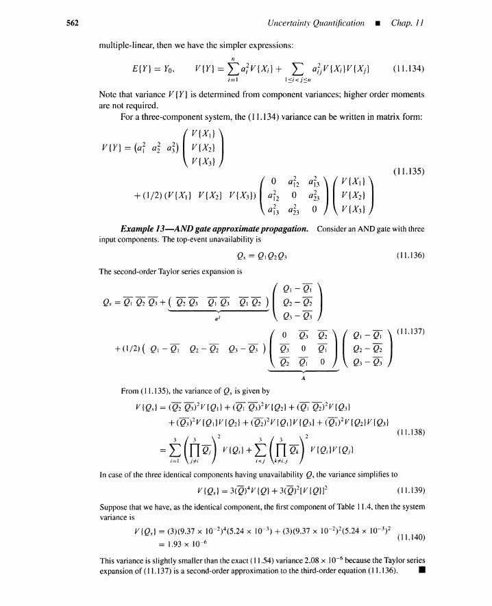
562 Uncertainty Quantification • Chap. II
multiple-linear, then we have the simpler expressions:
E{Y} == Yo, (11.134)
Note that variance V {Y} is determined from component variances; higher order momentsare not required.
For a three-component system, the (11.134) variance can be written in matrix form:
V{Y} == (a~ a~ a~) ( ~~~:~ )V{X3 }
+(1/2)(V{X1} V{X2} V{X3}) (012
a l3
(11.135)
Example 13-AND gate approximate propagation. Consider an AND gate with threeinput components. The top-event unavailability is
(11.136)
The second-order Taylor series expansion is
A
From (11.135), the variance of Q.\O is given by
V{Qs} = (Q2 Q3)2V{Qd + (~Q3)2V{Q2) + (~Q2)2V{Q3)
+ (Q3)2V {QdV {Q2} + (Q2)2V {QdV {Q3} + (~)2 V {Q2}V {Q3}
=t (u Qjr VIQ;l +t (p; Qkr VIQ;lVIQj)
(11.138)
In case of the three identical components having unavailability Q, the variance simplifies to
(11.139)
Suppose that we have, as the identical component, the first component of Table 11.4, then the systemvariance is
This variance is slightly smaller than the exact (11.54) variance 2.08 x 10⁻⁶ because the Taylor seriesexpansion of (11.137) is a second-order approximation to the third-order equation (11.136). •

Sec. 11.7 • Analytical Moment Propagation 563
Example I4-0R gate approximatepropagation. For a three-inputOR gate, (11.122)yields an expressionsimilar to (11.138), where unavailability Q is replaced by availability A:
(11.141)
Notice that the component availability variance is equal to the component unavailability variance,V {A;} = V {Q;}. This system unavailability variance is not exact because of the Taylor seriesapproximation.
The varianceis further simplified when the system unavailability expressionis approximatedby the first bracketof the inclusion-exclusion formula:
The Taylorseries expansionbecomes
(11.142)
yielding the varianceexpression
(11.143)
Consider an OR gate with three identical input componentswhose componentcharacteristicsare those in the first row of Table 11.4. The approximation (11.141) gives the system variance
V {Qs} = 3(A)4 V {A} + 3(A)2[V {A}]2
= (3)(1 - 9.37 x 10⁻²)4(5.24 x 10- 3) + (3)(1 - 9.37 x 10⁻²)2(5.24 x 10- 3)2 (11.144)
= 1.07 x 10- 2
while the first-bracket approximation of (11.143) yields
v{Qs} = (3)(5.24 x 10- 3) = 1.57 X 10⁻² (11.145)
•Example IS-SAMPLE tree approximate propagation. Consider the fault tree of
Figure 11.5 previously analyzedusing SAMPLE. The Taylorseries system unavailability expansionof (11.74) is

564 Uncertainty Quantification _ Chap. JJ
yielding the varianceexpression
V{Qs} = V{Qd + (Q3)2V{Q2} + (Q2)2V{Q3} + V{Q2}V{Q3}
= 5.24 x 10- 3 + (1.93 x 10- 1)2(9.28 x 10- 5) + (1.25 x 10- 2)2(2.20 x 10- 2) (11.147)
+ (9.28 x 10- 5)(2.20 x 10- 2) = 5.24 X 10- 3
Although the top-event unavailability is approximated by the first inclusion-exclusion bracket, theresult is in agreementwith the exact variance(11.100). Notice that (I 1.146) is an exact Taylorseriesexpansionof system unavailability approximation(11.74). Thus (11.147) is an exact valueaccordingto equation (11.74). Wecan conclude that the smallerSAMPLE variancein Table 11.5 stems from astatistical fluctuation due to a finite Monte Carlo sample size of 1200. •
11.8 DISCRETE PROBABILITY ALGEBRA
When a continuous probability density is approximated by a set of discrete probabili-ties, the uncertainty propagation can be modeled by discrete arithmetic [23-26]. Thisapproach can be regarded as a deterministic version of Monte Carlo, and is efficient foroutput functions with simple structures. Furthermore, the discrete probability approxima-tion is free from the random fluctuations inherent in finite Monte Carlo trials. Denote by{(PI , XI), ... , (P", Xn ) } a discrete approximation where Xi is a discrete value of variableX and Pi is a discrete probability. The approximation is performed under the constraint
n
LI1==1i=1
(11.148)
Consider a function Z == F(X, Y). Assume discrete approximations for variables Xand Y: {(11, Xi)} and {(Qj, Yj ) }. If X and Yare statistically independent, then the discreteapproximation for Z becomes
(11.149)
( 11.150)
The approximation for Z contains n2 pairs, thus the number of pairs increases rapidly as thepropagation proceeds, and pairs must be condensed or aggregated to avoid an exponentialexplosion.
Elementary operations among two different random variables include summation,difference, product, and ratio. Single variable operations include sum of a random variableand a constant, product of a random variable and a constant, product of the same randomvariable, and square root:
X+Y X-Y
Xx Y X/Y
X+C CxX
X n nConsider the output function Y == F(XI, ... , Xn ) . Two situations arise. If each
random variable appears only once in F, then the distribution for Y can be obtained bycombining two random variables at a time.
Example 16-Discrete algebra for nonrepeated events. Consider the outputequation
Y=X1X2/(X3+X4) (11.151)
Wefirstcompute V = Xl X2 and W = X3 + X4, and then Y = V / W.

Sec. 11.8 • Discrete Probability Algebra 565
If at leastone randomvariableappearsmore thanoncein F, then the expressionfor F has to bebrokeninto two parts, a part withoutrepeatedrandomvariables and one with the minimalexpressioncontainingrepeatedrandom variables. •
•(11.153)
These parts are then combined,yielding Y = V + w.
Example 17-Discrete algebra for repeated events. Consider the output equation
Y = Xl + (X2+ X3)(X4 + Xs) + X6 + X3X~/2 (11.152)
This expressioncan be dividedinto two parts:
V = Xl + X6
W = (X2 + X3)(X4 + X s) + X3X~/2
Note that four variables must be combined to obtain W. For complicated fault trees,discrete probability algebra becomes difficult due to repeated events; however, for outputfunctions with simpler structures, the discrete algebra, which is free from sampling errors,seems to be more efficient than Monte Carlo trials.
Colombo and Jaarsma [25] proposed discrete approximation by a histogram of equalprobability intervals. This has the following advantages: the intervals are small where thedensity is high and large where the density is low and combinations of equal probabilityintervals form equal intervals, resulting in a regularly shaped histogram that facilitates theaggregation of intervals. Figure 11.8 shows a histogram obtained by discrete probabilityalgebra with equal probability intervals [25].
160
140
120
100~0cQ)
80::::J0"Q)....l.L.
60
40
20
0
-
-
-
-
-
- I-
~
-......- ~
-
nI I
I I I I I I I
System Unavailability, 0/0
Figure 11.8. Histogramby equal probability intervaldiscrete algebra.
566
11.9 SUMMARY
Uncertainty Quantification _ Chap. 11
PRA engenders at least two sources of uncertainty: parametric uncertainty and modelinguncertainty. Parametric uncertainty involves statistical uncertainty and data evaluationuncertainty. Expert evaluation of component-reliability parameters results in extreme dataevaluation uncertainty. The Bayes theorem and log-normal distribution are used to quantifycomponent-level parametric uncertainty, which is propagated to the system level by methodssuch as Monte Carlo simulation, analytical moment calculation, and discrete probabilityalgebra. The resultant risk-curve uncertainty is crucial to PRA decision making.
REFERENCES
[I] Mosleh, A. "Hidden sources of uncertainty: Judgment in the collection and analysisof data," Nuclear Engineering and Design, vol. 93, pp. 187-198, 1986.
[2] "IEEE guide to the collection and presentation of electrical, electronic and sensingcomponent reliability data for nuclear power generating stations," New York: IEEE,IEEE Std-500, 1977.
[3] Apostolakis, G. "On the use of judgment in probabilistic risk analysis," Nuclear En-gineering and Design, vol. 93, pp. 161-166, 1986.
[4] Apostolakis, G., S. Kaplan, B. J. Garrick, and R. J. Duphily. "Data specialization forplant specific risk studies," Nuclear Engineering and Design, vol. 56, p. 321-329,1980.
[5] Mosleh, A., and G. Apostolakis. "Models for the use of expert opinions," presentedat the Workshop on Low-Probability/High-Consequence Risk Analysis. Society forRisk Analysis, Arlington, VA, June 15-17, 1982.
[6] Apostolakis, G. E., V. M. Bier, A. Mosleh. "A critique of recent models for humanerror rate assessment," Reliability Engineering and System Safety, vol. 22, pp. 201-217,1988.
[7] Swain, A. D., and H. E. Guttmann. "Handbook of human reliability analysis withemphasis on nuclear power plant applications." USNRC, NUREG/CR-1278, 1980.
[8] IAEA. "Case study on the use of PSA methods: Human reliability analysis." IAEA,IAEA-TECDOC-592, 1991.
[9] Zhang, Q. "A general method dealing with correlations in uncertainty propagation infault trees," Reliability Engineering and System Safety, vol. 26, pp. 231-247, 1989.
[10] Wu, J. S., G. E. Apostolakis, and D. Okrent. "On the inclusion of organizational andmanagerial influences in probabilistic safety assessments of nuclear power plants." InThe Analysis, Communication, and Perception of Risk, edited by B. J. Garrick andW. C. Gekler. pp. 429-439. New York: Plenum Press, 1991.
[11] USNRC. "Reactor safety study: An assessment of accident risk in U.S. commer-cial nuclear power plants." USNRC, NUREG-75/014 (WASH-1400), vol. I, 1975,appendix III, p. 104.
[12] Martz, H. F., and B. S. Duran. "A comparison of three methods for calculating lowerconfidence limits on system reliability using binomial component data," IEEE Trans.on Reliability, vol. 34, no. 2, pp. 113-120, 1985.
[13] Efron, B. "Bootstrap method: Another look at the jacknife," Annals ofStatistics, vol. 4,pp. 1-26, January 1979.

Appendix A.l • Maximum-Likelihood Estimator 567
(A.l)
[14] Depuy, K. M., J. R. Hobbs, A. H. Moore, and J. W. Johnston, Jr. "Accuracy of uni-variate, bivariate, and a 'modified double Monte Carlo' technique for finding lowerconfidence limits of system reliability," IEEE Trans. on Reliability, vol. 31, no. 5,pp. 474-477, 1982.
[15] McKay, M. D., R. J. Beckman, and W. J. Conover. "A comparison of three methodsfor selecting values of input variables in the analysis of output from a computer code,"Technometrics, vol. 21, no. 2, pp. 239-245, 1979.
[16] John, W. M. P. Statistical Methods in Engineering and Quality Assurance. New York:John Wiley & Sons, 1990.
[17] Meyers, R. H. Response Surface Methodology. Boston, MA: Allyn and Bacon, 1976.
[18] Kim, T. W., S. H. Chang, and B. H. Lee, "Comparative study on uncertainty andsensitivity analysis and application to LOCA model," Reliability Engineering andSystem Safety, vol. 21, pp. 1-26, 1988.
[19] Lee, Y. T., and G. E. Apostolakis. "Probability intervals for the top event unavailabilityof fault trees." University of California, Los Angeles, UCLA-ENG-7663, 1976.
[20] Jackson, P.S. "A second-order moments method for uncertainty analysis," IEEE Trans.on Reliability, vol. 31, no. 4, pp. 382-384, 1982.
[21] Cox, N. D., and C. F Miller. "User's description of second-order error propagation(SOERP) computer code for statistically independent variables." Idaho National En-gineering Laboratory, TREE-1216, 1978. (Available from NTIS, Springfield, Virginia22151 USA.)
[22] Cox, D. C., "An analytic method for uncertainty analysis of nonlinear output functions,with applications to fault-tree analysis," IEEE Trans. on Reliability, vol. 31, no. 5,pp. 465-468, 1982.
[23] Kaplan, S. "On the method of discrete probability distributions in risk and reliabilitycalculation: Application to seismic risk assessment," Risk Analysis, vol. 1, no. 3,pp. 189-196, 1981.
[24] USNRC. "PRA procedures guide: A guide to the performance of probabilistic riskassessments for nuclear power plants." USNRC, NUREG/CR-2300, 1983.
[25] Colombo, A. G., and R. J. Jaarsma. "A powerful numerical method to combine randomvariables," IEEE Trans. on Reliability, vol. 29, no. 2, pp. 126-129, 1980.
[26] Ingrain, G. E., E. L. Welker, and C. R. Herrmann. "Designing for reliability based onprobabilistic modeling using remote access computer systems." In Proceedings ofthe7th Reliability and Maintainability Conference, San Francisco, July 1968.
CHAPTER ELEVEN APPENDICES
A.1 MAXIMUM-LIKELIHOOD ESTIMATOR
Consider lifetime test data for n identical components. The test for component i is ter-minated after time lapse c., which is a "censoring time" determined in advance. Somecomponents fail before and others survive their censoring times. Denote by t, the lifetimeof component i, Define a new time Xi by:
{t., if t; ~ C;, i.e., failed components
Xi ==C;, if t; > C;, i.e., censored components

568 Uncertainty Quantification _ Chap. JJ
Introduce the following component notations:
f'(t: B)
r(t; B)
R(t; B)
probability density function
failure rate
reliability function
Denote by F and C the failed components and censored components, respectively.The likelihood L of the test data is defined as the probability density of obtaining the testresults when the distribution parameter vector B is assumed.
L(B) == nj'(Xi; B)nR(xi; B)iEF ;EC
(A.2)
The logarithmof likelihood L iscalled a log-likelihood. The maximum-likelihoodestimatorof parameter vector B is the one that maximizes the likelihood or equivalently, the log-likelihood I. Because J(t; B) == ret; B)R(t; B),
11
I(B) == In L == Lin rex;; B) + Lin R(x;; B);EF ;=1
The Weibulldistribution has the following failure rate and reliability function:
(A.3)
r(t; B) == Af3 (At )f3- 1, R(t; B) == exp[-(At)f3], (A == I/a) (A.4)
Denote by m the number of failed components in set F. The log-likelihoodcan be rewrittenas
11
to: (3) == mInf3 + mf3lnA+ (f3 - I) L lnx, - Af3 Lxf (A.5);EF ;=1
The exponential distribution has the f3-value of f3 == I, thus
11
to: I) == n11nA - ALXii=1
This log-likelihood is maximized at
" mA == ,,11
Li=IXi
(A.6)
(A.7)
A so-called Fisher information matrix is defined by a Hessian at the maximum-likelihood estimator O.
(A.8)
It is known that the maximum-likelihood estimator is asymptotically distributed with amultidimensional normal distribution; the mean is the true parameter value, while thecovariance is the inverse of the information matrix.
(A.9)
The second-orderpartialderivativescan beobtainedanalyticallyfor theWeibulldistribution.The maximum-likelihoodestimator is calculated by ordinary maximizationalgorithms. The
Appendix A.3 • Mean and Variance by Orthogonal Expansion 569
covariance matrix is then obtained as
(V{~}A Cov{~,,8} )=( VAA VA/3 )=I(~,/3)-l (A.IO)
Cov{ A, ,B} V {,B} VA/3 V/3/3
The variance of unavailability Q= I - Rit; ~,/3) can be evaluated from
V{Q} = ( aQ/a ~ aQ/a/3) (VAA VA/3 ) ( a~/a ~ ) (A.II)VA/3 V/3/3 8Q/a,B
A.2 CUT SET COVARIANCE FORMULA
The cut set covariance can be expressed as
Cov{Qj, Qk} = QjQZ - Qj QZ
This covariance can be rewritten in terms of basic-event unavailabilities:
A.3 MEAN AND VARIANCE BY ORTHOGONAL EXPANSION
(A.I2)
(A.13)
Let Z be a random variable with probability density p{Z}. Denote by o/k(Z) a kth orderorthogonal polynomial defined by
ifk = I
if k f. I(A.14)
The orthogonal polynomials up to the second order are given by
1 Z Z2Z Z2 Z31 Z Z2
0/2 (Z)
I~ ;1 I z Z2Z Z2 Z3Z2 Z3 Z4
(A.I5)
(A.I6)
(A. I?)

570 Uncertainty Quantification _ Chap. JJ
Introduce a normalized random variable Zi:
Z, == (Xi - Xi)/)V{X;}
Variable Z, has a zero mean and a unit variance.
(A.18)
(A.19)
Furthermore, the third- and fourth-order moments of Z, are the skewness and kurtosis ofthe original variable Xi, respectively.
(A.20)
(A.21)
The orthogonal polynomials for the normalized variable Z, are much simpler becauseof the normalized characteristics of (A.19).
1/Jl (Zi) == Zi
Z? - rR:Z· - 1'1/' (Z.) _ I "'P; I
,+,2 I - JYi - fJi - 1
From the orthogonal property of (A.14), we have
1/Jl (Zi) == 1/J2(Zi) == 0, (zero mean)
1/Jl(Zi)2 == 1/J2(Zi)2 == I, (unit variance)
1/Jl (Zi) 1/J2 (Zi) == 0, (zero covariance)
1/Jl (Zi)1/J2(Zj) == 1/Jl (Zi) 1/J2(~i) == 0, i i- j, (zero covariance)
(A.22)
(A.23)
(A.24)
(A.25)
The Taylor series expansion of (11.124) can be rewritten in terms of the normalizedrandom variable Zi.
n n
Y == Yo + LbiZi + (1/2) Lb;;zl + L bijZ;Zji=1 i=l l..si<j..sn
(A.26)
where coefficients b, and bij are given by
bi == ai)V{Xi}, (A.27)
(A.28)
The first-order terms Z, and the cross terms Z, 2.i can be written in terms of 1/Jl (Zi)
and 1/Jl (Zj); the second-order terms Z; can be rewritten in terms of 1/Jl (Zi) and 1/J2(Zi)'
z, == 1/J1 (Zi)
ZiZj == 1/J1 (Zi)1/Jl (2.i)' i i- j
Z; == )Yi - fJi - lVJ2(Zi) + jA1/Jl(Zi) + I
We have now an orthogonal expansion for (A.26):
(A.29)n
+ (I /2) L bi;)Y; - fJi - 11/J2 (Zi) + L bij 1/J1(Z i ) 1/J I (Zj )i=l l..si<j..sn
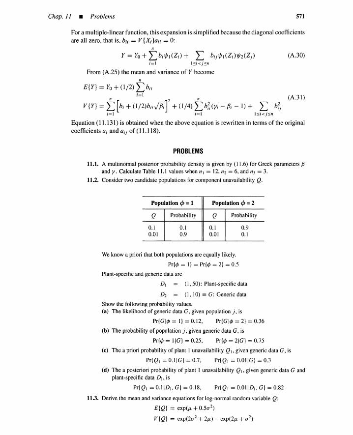
Chap. 11 • Problems 571
For a multiple-linear function, this expansion is simplified because the diagonal coefficientsare all zero, that is, b., = V {X;}a;; = 0:
n
y = Yo + Lb;l/!I(Z;) + L bijl/!I(Z;)l/!2(Zj);=1 I~;<j~n
From (A.25) the mean and variance of Y become
(A.30)
n
E{Y} = Yo + (1/2) Lb;;;=1 (A.31)n 2 n
V{Y} = L [bi + (1/2)b ii JA] + (1/4) Lb~(Yi - Pi - 1) + L b7j;=1 ;=1 I~;<j~n
Equation (11.131) is obtained when the above equation is rewritten in terms of the originalcoefficients a; and aij of (11.118).
PROBLEMS
11.1. A multinomial posterior probability density is given by (11.6) for Greek parameters f3and y. Calculate Table 11.1 values when nl = 12, n2 = 6, and n3 = 3.
11.2. Consider two candidate populations for component unavailability Q.
Population 4J = 1 Population 4J = 2
Q Probability Q Probability
0.1 0.1 0.1 0.90.01 0.9 0.01 0.1
We know a priori that both populations are equally likely.
Pr{<jJ = I} = Pr{¢ = 2} = 0.5
Plant-specific and generic data are
D1 (1, 50): Plant-specific data
D2 (I, 10) == G: Generic data
Show the following probability values.(a) The likelihood of generic data G, given population j, is
Pr{GI¢ = I} = 0.12, Pr{GI¢ = 2} = 0.36
(b) The probability of population i. given generic data G, is
Pr{¢ = IIG} = 0.25, Pr{<jJ = 21G} = 0.75
(c) The a priori probability of plant 1 unavailability QI, given generic data G, is
Pr{QI = O.IIG} = 0.7, Pr{QI = O.OIIG} = 0.3
(d) The a posteriori probability of plant I unavailability QI, given generic data G andplant-specific data D1, is
Pr{QI = 0.IID1, G} = 0.18, Pr{QI = 0.01ID1, G} = 0.82
11.3. Derive the mean and variance equations for log-normal random variable Q:
E{Q} = expu, + 0.5a2)
V {Q} = exp(2a 2 + 2J,t) - exp(2J,t + a 2)

572 Uncertainty Quantification • Chap. 11
11.4. Prove the maximum-likelihood estimator (11.64).
11.5. Consider a three-out-of-three valvesystem. Obtain a demand-failure probability expres-sion similar to (11.73).
11.6. Obtain two-dimensional Latin hypercube samples from the following sample data:
( ~2 4
3 I2 )5 '
(2 dimension, 4 strata)
11.7. Prove the inequality between AND and OR gate variance propagation.
V{QI /\ Q2} < V{QI v Q2} ifQI' Q2 < 0.5
11.8. Consider a two-out-of-threesystem. Evaluatesystem unavailabilityvarianceby momentpropagation through minimal cut sets.
11.9. Derive (A.23) and (A.24), that is, orthogonal polynomials for a normalized randomvariable.
egal and RegulatoryRisks
12.1 INTRODUCTION
Multimillion-dollar regulatory agency fines and hundred-million-dollar jury verdicts makegood headlines: here are recent samples stemming from product liability lawsuits and EPA,FDA, and OSHA (Occupational Safety and Health Administration) actions.
"EPA Sues Celanese for $165,000,000 for Air Pollution""Bard Medical Fined $63 Million by FDA""Ford Assessed $128.5 Million in Pinto Crash""EPA Fines Rockwell International $18.5 Million""Jury Assesses Upjohn $127 Million-70-Year-Old Man Loses Use of Eye""Chevron Hit with $127-Million Fine for Self-Reported Violation""OSHA Fines Phillips $5.2 Million for Explosion""Celotex to Pay $76 Million to Illinois 68-Year-Old in Asbestos Suit"
A plant shutdown due to an explosion or major failure is a catastrophe. A plantshutdown due to a lawsuit or a legal action taken by a government agency is an even moredebilitating event. In 1993 the EPA collected $130 million in fines and brought 140 criminalcharges, mostly against engineers. Currently, there are five to ten criminal charges againstengineers every week by the EPA alone. The risks of a legal disaster are real. In the UnitedStates there have been many more plant stoppages for legal and regulatory matters than foraccidents. There were 97,000 business bankruptcies in 1992. The number of Americanswho lose jobs due to their firm's legal and regulatory problems is orders of magnitudehigher than the number who lose their jobs due to industrial accidents. In 1992 the FDAcommandeered 2922 product recalls and prosecuted 52 people for violating its dictates.
In addition to strongly influencing profitability, legal and regulatory practices in-fluence product quality and plant safety. All countries have environmental and factoryinspection agencies that mandate engineering design and manufacturing practices. In ad-
573

574 Legal and Regulatory Risks • Chap. J2
dition, all countries have labor laws. These labor laws strongly influence the manner inwhich safety and quality control programs are structured.
It is naive on the part of engineers and scientists to focus only on technical matters.What industry can and cannot do is mostly decided, in the United States, by politiciansand lawyers. They run the legislatures, courts, and government agencies. It is incumbent,particularly on those who work in a field such as risk analysis-which has a large societalinterface-s-tounderstandthe legaland political processes that shape theircompanies' future,and to take an active role in influencing political decisions. Engineers must learn how todeal with government regulations and inspectors in order to reduce risks to themselves andtheir companies. Loss-prevention techniques should be developed.
12.2 LOSSES ARISING FROM LEGAL ACTIONS
In the United States, the risk of a company being crippled or closed down by lawsuits isfar from negligible. Billion-dollar corporations such as Johns Manville, Robbins, and DowCorning have been forced into bankruptcy by lawsuits. The light plane industry in Americais heading for extinction; Cessna reported legal costs of over $20 million in 1993-enoughto providejobs for 300 engineers. The American machine tool industry is dead, and nobodywith assets manufactures step ladders in the United States (if there are no assets, lawyer'sdon't sue: they only go after "deep pockets"). There are 1.24million lawyers in the UnitedStates-a world record. It is estimated they take $1.00 x 10¹² (one trillion dollars) out ofthe American economy every year. This is money that, in other countries, is used for plantmodernization, R&D, and for pay raises to workers. In 1992 liability awards and lawsuitsamounted to $224 billion, or 4% of the gross national product, according to the BrookingsInstitute. This is about four times as much as the total salaries of all engineers in the UnitedStates.
To understand what industries can do to reduce the risk and losses from lawsuits,one must first understand the nature of the problem and how it arose: a good starting pointis to read the book Shark Tank: Greed, Politics and the Collapse of Finley Kumble, OneofAmerica 's Largest Law Finns, by Isaac Eisler. Kumble, who was head of the country'ssecond largest law firm, had a favoritesaying, "Praise the adversary lawyer; he is the catalystby which you bill your client. Damn the client; he is your true enemy."
Americanattorneysare in the majority in the federal legislature,most federalagencies,and moststate legislatures. Usingslogans like"Consumer Protection,""Anti-Racketeering,"and "Save the Environment," they have made it incredibly easy and profitable to launchlawsuitsand to victimizecorporationsand rich individuals. Tortcosts to the medical industrytotaled $9.2 billion in 1994. Anyone doubting the fact that Congress makes laws that favorlawyers over industry and the public need only study the EPA'sSuperfund Program. Of the$20.4 billion spent thus far, according to the American Chemical Society, over $4 billionhas been consumed in legal and filing fees. Almost nothing is being cleaned up. Consumerprotection legislation has resulted in a similar mess. In the United States, litigious lawyersare paid not by their clients but by proceedsgenerated by suing the defendants ("contingencysuits"), which give lawyers incentive to win suits by any means possible. In Houston, a lawfirm whose telephone number is INJ-URED pays for late-night TV advertisements directedat "employees who want to sue their employers... no fee charged."
An even greater abuse is that a company subject to an extortion-type lawsuit, and thatwins incourt, cannot recoverits legalfees. Lawyersadvertise widelyandaggressivelysolicit

Sec. 12.2 • Losses Arising from Legal Actions 575
clients. The situation is further exacerbated by the fact that lawyers "own" the courts, thatis, the courts are run by lawyers for lawyers. Trials last for years, and sometimes decades,and cost from $50,000 to tens of millions: the average product liability lawsuit runs for 2.4years. It is "against the law" for a person or a company to represent themselves in court,that is, judges force defendants to hire lawyers. It is a classic loss-prevention problem.
There are various types of lawsuits: although they pose greater and lesser risks tocorporations, all cost money and resources. To quote R. J. Mahoney, president and CEO ofMonsanto Chemical, "The legal system exacts a crushing cost on our way of life."
12.2.1 Nonproduct LiabilityCivilLawsuits
This type of lawsuit arises from alleged mistakes made by company employees thatcause damage. The $124-million award to a $93,000-a-year financial officer for wrongfuldischarge by a southwestern energy company was a civil lawsuit outcome. An automobileaccident can bankrupt a medium-sized company if one of their trucks hits a school bus andhurts a number of children, because liability insurance, which typically is a few milliondollars for a medium-sized company, will never be adequate. Furthermore, lawyers whospecialize in automobile accident lawsuits will ask triple and punitive and exemplary dam-ages because the company, according to the plaintiff's lawyer, failed to properly train andsupervise and discipline their drivers. Exxon's multibillion-dollar Alaskan oil spill fine isa case in point. The captain was said to be drunk. The company is helpless to defend itself,even if it has an expensive training program; after all, an accident did happen.
It is noteworthy that the court papers and official charges served the defendant in alawsuit, although signed by the court, are prepared by the plaintiff's lawyer for the judge'ssignature. The most outrageous charges are levied with no judicial review whatever. Theproblem this raises is that the judge, by signing these types of charges, has given theplaintiff's lawyer unlimited license to harass a company. For example, a plaintiff's lawyercan ask for financial, sales, personnel, and engineering records even though he or she issuing the company because their client slipped on the sidewalk and twisted an ankle. Thisis because included in the charges signed by the judge is the accusation of "willful neglect"and a request for "compensation" and "triple damages." The harassment is sanctioned bythe judges on the grounds that the plaintiff's lawyer is entitled to know how much moneythe defendant has so it can be decided how much money to sue the company for. This typeof harassment is called discovery and generates massive paperwork and legal fees.
Civil lawsuits, if properly handled, are usually not a major risk for a company becausethis type of lawsuit is usually not too costly and is customarily insured for. An exception,of course, is liability arising from the type of sabotage (accident) that befell Union Carbideat Bhopal, India. If this had happened in the United States, Union Carbide would surelynow be in Chapter 11 bankruptcy. The utilities that ran the Three Mile Island reactor werenot bankrupted because they have a statutory monopoly and can raise electricity rates.
12.2.2 Product Liability Lawsuits
Here is the ultimate nightmare. Johns Manville was bankrupted by asbestos lawsuits,and Robbins by lawsuits relating to intrauterine contraceptive devices. The onslaught oflitigation in America relating to intrauterine contraceptive devices was such that, althoughthey are still used and available everywhere else in the world, all American manufacturerswere forced to discontinue production. The legislation relating to product liability lawsuitsis so unfavorable to industry that entire industries that make products frequently involved

576 Legal and Regulatory Risks • Chap. J2
in consumer or industrial accidents (ladders, machine tools, etc.) have not been able tosurvive the avalanche of lawsuits by people who use (or misuse) their products. Only onemanufacturer of vaccines survives in the United States. An additional problem relating toproduct liability lawsuits is that of a product recall, which a company may decide to initiatevoluntarily or may be forced to initiate by a government agency. FDA-mandated recallsof medical devices totaled nearly 3000 last year. Product liability insurance in the UnitedStates costs 20 times more than in Europe and 15 times more than in Japan. The GAO(Government Accounting Office) estimates that 60% of the product-liability awards go toattorneys.
It will be interesting to watch the trauma relating to the silicone (and saline) breast-implant controversy. In 1993 a Texas jury awarded one woman $27 million because theimplant allegedly damaged her immune system and she became arthritic. Since then therehave been eight scientific studies, including one large one sponsored by the PHS (PublicHealth Service) showing no relationship between breast implants and connective tissuediseases. So many lawsuits take place in Texas because it is the only state that permits civilcharges to be filed irrespective of where the alleged act took place; and because Texas judgesare elected, over 80% of their campaign contributions come from lawyers! Multiply the $27million by four million, which is the total number of women who are said to be consideringlawsuits (or who have already launched them in response to large newspaper, TV, andbillboard advertisements by lawyers), and one cannot be too sanguine of the survival, intheir present form, of premier corporations like Dow Chemical (Dow-Coming has alreadypleaded bankruptcy) and Bristol Myers Squibb. Pity their employees; both companies haverecently announced large layoffs; a five-billion-dollar reserve fund was set up to coverlosses.
12.2.3 Lawsuits byGovernment Agencies
In their zeal to further the cause of their back-home law partners, and at the behest ofthe strongest and richest of all lobby groups, the Trial Lawyers' Political Action Associa-tion, Congress-the majority of whom are lawyers-has given nearly all federal agencies(OSHA, FDA, NRC, EEOC, EPA, etc.) the right to level fines against industries and tolaunch lawsuits (including criminal proceedings) against companies and their employees.One result of these laws is that if a manufacturer has the bad luck to have an accident, it canbe almost certain that one or more government agency will sue and/or level a large fine-always after the fact. Phillips Petroleum, CONOCO, and ARCO, for example, were finedmillions by OSHA after they had plant explosions, despite the fact they easily passed OSHAinspections just prior to the accidents. Dr. Homsley, who was making artificial implants forover a decade in Houston, and who passed FDA manufacturing inspections yearly, suddenlywas shut down and taken to court by the FDA for violating good manufacturing proceduresafter an implant failed. He closed his factory, declared bankruptcy, moved to Switzerland,and opened a new factory, after publicly denouncing the FDA for their Gestapo tactics. Theauthors' personal experience with OSHA, EPA, and FDA inspectors is that the fines andseizures are mostly the result of company employees reporting to inspectors that there wasa product failure and that it had been voluntarily corrected. The government inspectors, bythemselves, seldom find anything seriously wrong in routine inspections.
Government fines, even when they are as high as the $18.5-million fine levied againstRockwell International, traditionally are less than it would cost to defend the company incourt against a federal lawsuit, so nearly everyone pleads innocent and then pays reduced
Sec. 12.2 • Losses Arising from Legal Actions 577
fines. The net result, however, of this government prosecution of companies who havehad the misfortune of experiencing a major accident or lawsuit is that the government aidsand abets the cause of all the lawyers who-as a result of the accident-file legitimate(or fraudulent) civil lawsuits against the company because the government agencies, bytheir fines, have branded the company as criminal. An excellent example is the SuperfundProgram. In Riverside, California, an EPA lawsuit was followed by a civil suit on behalf of3800 plaintiffs targeting 200 companies.
There is a misconception by a segment of the population that government inspectorsand regulators are impartial servants of the people. This is most certainly not a universaltruth. The pressure is on the inspector to find violations, whether they are justified or not.
Mendacity is a prevalent human trait; every survey taken shows that about 85% ofcollege students and over 90% of high school students cheat at some time or another.The statistical distribution of people who are willing to stretch the truth is the same in thegovernment as everywhere else. Company employees who deal with government inspectorsmust be made aware of this and be rigorously trained to do nothing other than answerquestions laconically. The buddy-buddy approach is dangerous and puts the company atrisk.
12.2.4 Workers' Compensation
Losses due to workers' compensation payments are so large they deserve specialattention. In theory, workers' compensation insurance provides medical care and, if nec-essary, disability payments to workers who suffer job-related injuries. The fact that thecompany mayor may not have generous health insurance policies and benefits for theirworkers is not pertinent: Workers' compensation is required in all states. In America,workers' compensation laws vary dramatically from state to state and can result in anythingfrom a major to a moderate expense. In Texas, for example (where lawyers specializing inworkers' compensation, according to legislative testimony, make yearly incomes in the $1to $3 million category), an ex-employee can sue an employer for physical disability as longas one year after he or she worked for that employer. It is generally agreed that there is atleast a 25% fraud factor in workers' compensation claims.
In most states, it is traditional for larger corporations to self-insure against the risk ofworkers' compensation lawsuits. The cost is high ... about 1% of the sales in Texas in 1991:in the oil service business, premiums averaged $30 per $100 of payroll costs in 1990. Themechanism of self-insurance, by law in most states, is to pay the premium to an insurancecompany, who administers the program. The insurance companies invariably do safetycompliance inspections and insist that the company have a full-time safety department,independent of size, thus generating further industry expense.
About half of workers' compensation payments are for medical costs, the rest fordisability payments. Lower back claims, which, in a carefully rehearsed person, are impos-sible to refute, accounted for $11 billion (40%) of workers' compensation payment in 1993.The average cost of back pain is now $24,000, and the standard insurance company reserveis $80,000 per case. The National Center for Health Statistics tells us the two million carpaltunnel claims average $29,000 each!
In 1992, when a Houston company instituted company-wide drug tests the employeeswere given sixty days to clean up. Two days before the drug tests were to begin, fiveworkers filed workers' compensation claims for back injuries. One of them had a trafficaccident on the way to the workers' compensation office and was found by the police to
578 Legal and Regulatory Risks • Chap. J2
be under the influence of drugs. Nevertheless, he, with the help of his lawyer, won theircompensation/disability claim. Workers' compensation was originally created to benefitworkers who were the victims of industrial accidents but, due to an onslaught of litigation,disability and medical payments are now being awarded for all types of personal aberrations(anxiety, depression, mental anguish, even obesity) because of alleged job-related stressabove and beyond that related to domestic stress.
In most states workers' compensation cases involve quasi-judicial proceedings thatdo not end up in the courts. However, it is highly advisable to keep excellent employeehealth records and to contest all claims, particularly when the employee is representedby a lawyer. Company personnel should be trained to testify at workers' compensationhearings; the stakes are very high; loss prevention scenarios must be developed. Workers'compensation expenses exceed engineering budgets at many companies.
12.2.5 Lawsuit-Risk Mitigation
A naive viewpoint is to hypothesize that if a company does exhaustive manufacturing-risk and product-safety studies it will be immune from-or will win-liability lawsuits. Avery contrary view was recently given by a high official of one of the most socially respon-sible of the large international companies. His hypothetical point was that, in an Americancourt, a better defense than producing safety studies (which imply that the company madethe studies because they felt the product or process was risky) is to deny any corporateknowledge that any safety problem ever existed. One can draw whatever conclusions onewants, but the consensus of experienced lawyers would be that if the only reason for doing a
. risk analysis is to generate paper and information that would be useful in a liability lawsuit,then this activity is a waste of time and money.
It is pitiful to note that testing and approval of products by government agencies suchas the FDA, DOT, and PHS (Public Health Services), or the strongest of warning labelsaffixed to the product, are no deterrent to lawsuits. IUD devices and breast implants, forexample, were FDA-approved for sale. Warning labels on cigarettes, which are monitoredby the PHS, have not stopped lawsuits against tobacco companies. GM truck designs meetelaborate government safety requirements and DOT test standards, yet the company wastabbed by a jury for $99 million for willful negligence.
There is no geographical escape from lawsuits generated by federal agencies; however,product liability, general liability, and workers' compensation laws vary from state to state,so corporate location is important. In New Jersey, for example, workers' compensationlaws are favorable to employers, and insurance costs are a small fraction of what they are inTexas. The difference in cost is because New Jersey has fixed schedules of payments andthe process does not involve lawyers.
In the last five years, a number of states have passed tort reform laws to help companiessurvive product liability lawsuits. These laws, for example, do things such as limit thenumber of years, after sale, that a manufacturer is responsible for his products. Right now,in most states, manufacturers are unindemnified in perpetuity, even though the product hasbeen repaired, rebuilt, and modified by users many times.
The ultimate-perhaps the only-way of avoiding the risk of American lawsuits isto become a truly international corporation. Dow Chemical, for example, which has halfof their sales and manufacturing facilities outside the United States, reports that more than90% of their total legal/insurance/lawsuit expenses arise in the United States. Increasingly,the chemical industry is moving overseas to lower, among other things, the risk of actions

Sec. 12.2 • Losses Arising from Legal Actions 579
by government agencies and to avoid a costly, unfavorable legal climate. Employment inthe U.S. chemical industry has dropped by more than 15% this decade, despite the factthat total worldwide employment by the industry increased almost by a factor of 1.5. Thechemical industry has almost completely stopped all investment in new U.S. manufacturingplants.
The RobbinslManville case and other such cases demonstrate that insurance cannotsave a company from the thousands or tens of thousands lawsuits that might spring up-asthey will in a product liability situation. For lawsuits other than massive product liability,risk mitigation is best practiced by settling out of court, that is, before the jury trial starts.Probably as many as 98% of all lawsuits that are filed are settled before they go to trial:over 900/0 of all lawyers in the United States have never been in a courtroom or tried acase. They rely on the fact that the defendant knows that a trial will be costly, so theycustomarily accept a payoff less than projected defense costs. Most lawsuits are settledout of court for $5000 to $10,000, even though the plaintiff initially asks for hundredsof thousands or millions of dollars and a jury trial. At best, lawsuits are an unsavory andunproductive activity for everyone except lawyers. At worst, they represent open and nakedextortion by a group that controls the courts, and are able to force defendants into no-winsituations.
12.2.6 Regulatory Agency Fines: Risk Reduction Strategies
The "fineiest" of all agencies, in the author's experience, is OSHA. . .. Their in-spectors do not like to leave the premises with empty pockets. In 1983, the agency levied$4 million in fines, a number that avalanched to $120 million in 1994. Over half of the$120 million was for errant paperwork, not industrial safety violations. Like the EPA andFDA, the agency does not lack for personnel; one documented case involves a disruptivefour-month visit to a chemical plant by a team of seven OSHA inspectors. In all, the federalregulatory bureaucracy employed 128,615 people in 1993.
In 1993, an OSHA inspector, unable to find anything else, fined our company $175 fornot having an employee-signed Material Data Safety Sheet for a can of store-bought, WD-40 lubricant that the inspector spotted in a plumber's tool kit. It is pathetic that regulatoryagency heads do not recognize that actions such as these promote hostility, not industrialsafety. Small wonder that, in a recent survey by the Heritage Foundation, both employeesand owners of businesses, by a two-to-one margin, viewed the government as an opponentrather than a partner in their pursuit of the American dream.
Although it is not immediately cost effective to fight a $175 regulatory agency fine,from a long-term risk management standpoint all violations should be contested, through atleast one regulatory agency management level. The most effective course of action is to hirean in-state (not Washington) regulatory consultant to help prepare the appeal and accompanycorporate technical people to the hearing, if there is one. Typically, these consultants areex-agency employees who are on a first-name basis with the local field office employees andare familiar with agency politics and policies. It is a grave mistake to hire an attorney fora first-round appeal. Not only will the cost be much higher, but one is more likely to lose,because lower-level agency employees, who are likely to be engineers or science-degreed,don't like any lawyers, including their own agency's because, if nothing else, the lawyer'ssalaries are much higher than theirs. In dealing with the FDA, our company once made thenaive mistake of hiring a Washington law firm to contest a product-recall violation. Twomonths and $15,000 in legal fees later, we had made no progress, so we fired the lawyer.

580 Legal and Regulatory Risks • Chap. J2
The agency people we were dealing with, who refused to talk with us as long as we had alawyer, suddenly became very friendly, and settled the violation without a fine.
Once a matter is in the courts, one has no choice but to hire a lawyer. Althoughthere appears to be no law against it, judges, in our experience, will not let a corporationrepresent itself in their courtrooms, even if it is abundantly clear that attorney costs willexceed any possible damage award. Some government agencies, the Commerce Departmentin particular, refuse to give information to anyone except an attorney. "Have your attorneycall us," is what they tell you. In 1991, the Commerce Department levied an export/importban on a small Dutch company, Delft Instruments, for allegedly selling bomb-sights toSaddam Hussein. It took over a year and $10,700,000 in fees to a gang of Washingtonattorneys to have the export/import ban lifted. By then, of course, the business was lost.Careful cost/benefit studies should precede all legal actions: that's the lesson here.
12.3 THE EFFECT OF GOVERNMENT REGULATIONS ON SAFETYAND QUALITY
The single most important goal of a government bureaucracy is to perpetuate itself and toannually convince the legislature to give it more: more people, more power, more money,and greater jurisdiction. A prime example is the U.S. Census Bureau, whose only legitimatemission is to do a head count so that congressional seats can be properly appointed. Overthe years, ambitious directors of the census have convinced Congress to expand the scopeof their operation to a point where the bureau spends $2 billion sending out, collecting,and tinkering with complicated questionnaires that are largely, if not mostly, not returned,or incorrectly filled out. Considering the fact that 22% of the population is functionallyilliterate, the accuracy of the census bureau data can never be better than a guesstimate. Thejob could be done,just as accurately, by counting drivers' licenses and/or voter registrations,because a very large fraction of all census questionnaire answers are computer-synthesized.After every census, states, counties, and cities challenge the census results in court, chargingthat the information is incorrect.
The history of agencies created to hold industry's feet to the fire, vis-a-vis workplacesafety, consumer protection, job discrimination, environmental protection, and restraintof trade, is not much different from the census bureau's. A case in point is the EEOC,the Equal Employment Opportunity Commission. Originally organized to enforce equalrights for minorities, the scope of the agency was then expanded to include women, andin 1992 expanded even more to assure equal rights in the workplace for disabled workers;in 1993 the Family Leave Bill was passed, which gives lawyers incredible powers to suefor damages above and beyond any personal loss. It is ironic that until 1995, Congress,which employs 12,000 people, has exempted itself from all equal opportunity and laborlegislation, including the Family Leave Bill.
As the Census Bureau, which can't get the count right (they invariably "find" a muchhigher percentage of women than is known to exist), the EEOC has a great deal of difficulty"putting it together," so to speak, because "discrimination," "handicapped," and so on aresubjective concepts that defy qualification. Nearly every alleged case is controversial andpotentially represents a lawsuit because not only is the EEOC empowered to sue and finea company, but so is the employee. A reasonable guess would be that about 5-10% ofall people fired by industry end up suing their employer, and if the person is a minority, afemale, handicapped or elderly, the risk of a lawsuit rises to 1D-20%-except in the case

Sec. 12.3 • The Effect ofGovernment Regulations on Safety and Quality 581
of plant closing, mass layoffs due to retrenchment, or a prelawsuit settlement of some sort.Engineers, most of whom are in supervisory positions, must learn to protect their companiesfrom this type of risk and subsequent losses.
12.3.1 Stifling of Initiative and Abrogation ofResponsibility
There is another characteristic of government that has unfortunate consequences forindustry. Government bureaucrats strive to compartmentalize and routinize everything.State air quality control boards, for example, use the same reporting and site approvaland pollutant dispersion forms for chemical plants, breweries, and electronic assemblyplants. If a company wants information on acceptable abatement technology, the standardagency approach is to give the applicant a list of registered and approved consultants andvendors. The people on the approved list always recommend standard technology. If acompany needs to reduce ethylene oxide emission, for example, the agency will refer themto vendors who sell incinerators and acid absorption systems. The possibility of novel ideasand new solutions to old problems is thus greatly reduced. The safest, most prudent, andmost economical course of action for any company is to say "yes, sir" and do anything thatthe government agency tells them to do. Appeal processes take so much time, money, andmanpower that irreparable harm is done to the company.
Every government agency has a large legal staff. Reliance on the courts is hopeless;this takes years. If the FDA sends one of their infamous" I5-day," comply-or-else letters, itwould be suicide for a company to say "I won't comply... the violations cited by your agencyare stupid and are the result of a plant inspection carried out by a semi-literate inspector whohas no technical training whatsoever, and who has not the remotest understanding of mycompany's complex technology, business, products, or customers." The result of ventingone's frustration in this impudent manner is a certain plant shutdown, no less costly than amajor fire.
As organizations such as the FDA, NRC, OSHA, and EPA (all of whom are chargedwith regulating workplace safety) mature, they produce increasingly detailed reports, ques-tionnaires, SOPs (standard operating procedures), and safety requirements. Permissiblechemical and radiological exposure limits, as well as top-event risk standards, are set bygovernment agencies. It would be unthinkable for anyone to apply for an air quality controlboard (AQCB) permit for a site expansion and not to categorically swear that every singleagency requirement will be met. A company is no more than a collection of individu-als: people, not companies, fill out site-application forms. When people make mistakes,the company pays dearly. As was pointed out earlier, 85% of college students admit tooccasional or systematic cheating.
Given this natural state of the human being and the pressure of the workplace, is itany wonder that when the government issues technically or financially unattainable require-ments, frequently one of two results occur? Marginal producers with minimal assets willmeet the requirements on paper. They base future survival on the same set of premises as adriver who does 60 mph in a 55-mph speed zone; detection of the violation is uncertain, thepenalty is manageable, and an excuse may work. Well-managed, technologically strongcompanies will locate new plants off-shore and run old ones as long as possible.
Totalitarian countries and welfare states are characterized by a lack of personal initia-tive and unwillingness by individuals to take responsibility for their own actions. Personalresponsibility ends when what the government asks to be done has been done. As the gov-ernmental agencies become more and more specific in what they require in the way of safety
582 Legal and Regulatory Risks • Chap. J2
studies, safe operation, and worker training, the safety engineer's attention and energies arediverted from creating an active safety program and become focused entirely on meet-ing government requirements and creating documents that satisfy armies of governmentinspectors.
When the NRC decrees that all reactor operators shall have five hours of trainingper month, the name of the game changes. Focus shifts from creating an active safetyculture to one of creating, scheduling, and implementing a program that lasts for five hoursper month, and is in passive compliance with NRC's training directives. If, because ofa personnel department error, training-session attendance had not been recorded into anoperator's personnel folder at the time of a government inspection, the company is subjectto fines and court actions whether or not they have an excellent safety record and trainingprogram. When dealing with regulatory agencies, forrn invariably triumphs over substance.Emphasis is totally on the process-the product does not matter. In regulatory agencies runby lawyers, words are more important than actions.
12.3.2 Overregulation
The most lawless countries have the greatest number of laws. In 1964 the Braziliangovernment passed 300 major laws in one day. Clarity, purpose, and effectiveness werecompletely overshadowed by political posturing and enlightened self-interest. The lawswere largely unenforceable and unenforced: as with the American prohibition, or "nospitting on the sidewalk." When the Brazilian government passed a law in 1965 that allprofessors at federal universities must be "tempo integral," that is, full-time professors, atourist or naive citizen might have proclaimed "university reform is finally here." Thatwas not the case at all. There had been three previous such laws, all unenforced and allunenforceable. The Congress of the United States has put an anti-business weapon in thehands of lawyers called the RICO (racketeering-influenced and corrupt organization) law.It is cited by plaintiff attorneys in tens of thousands of lawsuits against honest corporationsand organizations. It is so vague that it has never been properly defined: the cases involvingalleged violation of this law are won or lost on other, more substantive issues. Lawyers liketo cite it because it has a triple-damage provision, which gives them enormous power toharass defendants. Interestingly enough, this racketeering law has been used successfullyto sue anti-abortion groups who block women's access to abortion clinics.
The net result of overregulation is that nobody knows what the law really is andindustry is at the mercy ofjudges and government inspectors. Company management mustfocus on sales and manufacturing if it is to survive in a worldwide, competitive businessclimate. When a fire inspector struts in and demands a complete reorganization of thecompany's warehouse because-he says-the code prohibits stacking closer than one footfrom the ceiling, who knows whether he is right or wrong? There are different codes inevery city and county. This also applies to the tax code. Companies doing business in all 50states are inspected by revenue inspectors from each of these states (as well as the federalgovernment) and are expected to know everyone of the nation's millions of city, state, andcounty tax law regulations. This is the same situation a citizen faces when dealing withan IRS inspector. Nobody has read and understood the entire tax code. The IRS inspectorpretends to know the code, so the citizen is wrong. Legal precedents are invariably toonarrow or nonexistent. The IRS, when challenged in court, lost 70% of the cases, but fewhave enough money to fight the IRS.

Sec. 12.4 • Labor and the Safe Workplace 583
Human beings and organizations do not function well under uncertainty. When itbecomes impossible to know and understand the laws that pertain to your business, andwhen armies of government inspectors have the right to issue fines and summonses, andthe corporation is immediately declared guilty as charged and must post fines until, atenormous expense and lost time, it proves itself innocent, then safety and reliability studieswill not capture the attention of upper-level management, because they don't relate toimmediate survival issues. The up-front investments in quality, safety, and reliability arehigh, and funds may not be available. The Wallace Corporation, which in 1990 won theCommerce Department's prestigious Malcom Baldridge National Quality ManufacturingAward, declared bankruptcy in 1991.
12.4 LABOR AND THE SAFE WORKPLACE
Consider what has happened in the public school system; probably the most regulated ofthe American workplaces. Magnetic weapons-inspection systems, barbed-wire fences, andsecurity guards characterize many public schools in major cities. Undue focus and energyare put on dealing with the problems of system deviates. Management focuses on quellingdisturbances rather than furthering the common good. The cost and manpower required tocomply with government DOE (Department of Education) regulations is staggering. Eachschool district, by law, must retain professionally trained arbitrators assigned to mediatebetween parents of handicapped students and the district to assure complaining parents thatthe school has provided enough facilities and special programs to meet the needs of the child,the parents, and whatever advocacy group chooses to intervene. The school is mandatedto provide the "least restrictive environment" for all disadvantaged students. Dyslexiaand very low mental ability are considered handicaps, and such students are given specialentitlements. Specialists in sight impairment, speech impairment, and general learningdisabilities must, by law, be in place. All of this extracurricular effort requires extraordinaryamounts of money and effort. School taxes have increased an average of 6.5% per year in theUnited States during the past 15 years, largely to pay for the costs ofnew programs mandatedby the state and federal departments of education. Some of these increased expenditureshave been used to pay attorneys who are suing the district on behalf of aggrieved parentsor special interest groups. The city of Houston recently had a special election to raise$15 million to pay for unbudgeted legal bills. A quote attributed to Lee Iacocca, when hewas the president of Chrysler, was "no matter what we budget for legal costs, ·it is neverenough."
During the past two decades the educational community has witnessed an enormouseffort on the part of the government to educate the population in civic tolerance----definedas the adoption of the viewpoint that no person is a liability to the community, regardlessof their negative contributions to society. By implication, industry also is being pushedto "forgive and forget" and to automatically promote people in the same way the schoolspromote people, and pass students from grade to grade regardless of achievement.
The government has spent billions creating protected groups within the educationaland public economic sectors. This enormous effort to create protected groups has failedboth the majority and minority sectors of the population. In 1992, under the pseudo-idealistic guise that all people should have equal opportunity and access to employment,politicians seeking to strengthen and expand their political base extended the economically

584 Legal and Regulatory Risks • Chap. J2
damaging concept of protected groups to private business, completely neglecting the factthat private industry, unlike public schools, cannot arbitrarily raise their prices 6.5% everyyear. Their European and Asian competitors are not forced to hire protected groups andare free to dismiss disloyal and unproductive employees without being brought to court bygovernment agencies and contingency lawyers.
To use an analogy from athletics, the educational establishment and industry forma relay team. The baton that the educational establishment passes to the industry is thelabor force. Twenty-two percent of this labor force is illiterate; in much of the country ithas sprung from an environment where school absenteeism is as high as 25%, in whichthere is no punishment for poor performance or poor discipline, and people are trainedto take advantage of protected-group and litigious advocacy situations. The baton beingpassed to industry consists of the most poorly educated work force (in terms of academicachievement) of all the industrialized countries in the world. The creation, under theseconditions, of an effective, viable, corporate safety culture is a challenging task.
12.4.1 Shaping the Company's Safety Culture
Embedding a safety culture into the diverse ethnic and cultural group that comprisesthe American work force is a difficult, but certainly not impossible, task. It involvescarefuland patient management and realization that, from the standpoint of education, it involvesboth learning and unlearning. A new employee who has, in his 12 years of schooling,learned nothing but how to cheat and beat the system must be taught that now he is thesystem. If that cannot be done, and done very quickly, the employee should be terminated:there is no reasonable statistical hope of rehabilitation. This is a point repeatedly stressed byJoe Charbonneaux, one of America's most popular and successful management consultants.His seminars and courses on effective corporate management stress the concept that 27% ofall company employees contribute negatively to productivity and have poor attitudes towardtheir work and their company, and that there is absolutely nothing that the company can doin the way of education or training that will change them or their behavior. The title of hismost popular seminar is "Look Who's Wrecking YourCompany."
The first step in setting a successful course is to recognize the obstacles ahead and toprepare to overcome them. This starts with the hiring process.
12.4.2 The Hiring Process
At the University of Houston, as at most universities, students are asked to commenton and rate all courses at the end of each semester. In the 1994 senior design course wherethe students worked in teams of four, one of the students offered the following comment:"What I learned in this course is that it is not possible to produce a good design when yourcoworkers are stupid and lazy." This may be the most valuable lesson he learned in his fouryears of college.
Considering the major responsibilities given risk, safety, and loss-prevention man-agers, it is very reasonable that they have a voice in the hiring process. Hiring decisions aretoo important to be left solely to the human resources (employment) departments. Thesedepartments are frequently more focused on avoiding EEOC fines and lawsuits (whichwould reflect badly on them) than on the risk taken by hiring someone who is dyslexic andmight blow up the plant (which would reflect poorly on the risk manager).
A case in point is that the government, on the pretext of national security, is permittedto screen employees in a manner forbidden to industry. Under the 1990 Americans with

Sec. 12.4 • Labor and the Safe Workplace 585
Disabilities Act (ADA) regulations, which Representative Richard Armey estimates willcost American industry $100 billion in the next five years, it is felony-level violation toask any question relating to the job history of applicants (whether or not they fall into theprotected group category).
Clearly, anyone with a learning disability that leads to impaired judgment or physicaldisabilities such as uncontrolled seizures or tremors puts all of his or her coworkers at risk inmany job categories. The next point to note is the type of psychological mind-set or deviantbehavior that makes people accident-prone. Among these are failure to understand, failureto read instructions, failure to seek advice, inability to make decisions under pressure, andlosing ability under stress.
There are proven psychological stress tests used by the airline industry for testingpilots that provide excellent indicators of accident-proneness and inability to function understress. Tests of this type should be given to operators of complex and dangerous plants andequipment. Drug testing must be compulsory. The rate of workplace drug abuse in 1992(at companies that do drug testing) was 8.81 %, with marijuana accounting for 39.5% ofthat amount.
Because of the high rate of (at least) one remission following drug rehabilitation(estimates as high as 65 percent have been published), the best drug policy, from a risk-aversion and cost-control standpoint, is universal, mandatory drug testing with immediatedismissal of any company employee failing a drug test. If uniformly applied, this policyis completely legal and less likely to engender costly lawsuits than vacillatory programsinvolving rehabilitation. Exxon, for example, has a policy allowing employees who faildrug tests to enter drug rehabilitation programs and continue to work, and is now fightinga class action lawsuit by "rehabilitated" employees who claim they were not promoted asquickly as people who did not have drug abuse histories. Engineers responsible for lossprevention and operations should demand their companies have strict, uncompromising,drug programs. Drugs distort judgment: drug abusers are as dangerous as drunken driversand should not be tolerated in jobs where their actions can cause harm to others.
Poor judgment and mental instability have certain associated indicators such as poordriving and accident records, credit problems, and possibly a criminal record. Driver licenserecords as well as school records should be examined by the risk and safety directors toestablish whether or not errant tendencies, which put people and the plant at risk, can bedetected.
Many employers ask job applicants to take the Wonderlic Personal Test. This test isinternationally recognized as a standardized measurement of general cognitive ability. Itrequires no factual knowledge above what one learns by the sixth grade. Cognitive abilityis, of course, a test prerequisite, but in most countries it is also a prerequisite for even thelowest-level industrial job. There are fifty questions; the average score for all job applicantsis 21, which is also the average score for high school graduates. College graduates average29; only 0.0034% of the people who take the test achieve perfect scores. The standarddeviation of the Wonderlic is 7.12.
Because the Wonderlic test has been given to millions of people, it is possible toobtain precise correlations between scores on the test and age, ethnicity, schooling, and jobfunction. The following observations can be made (source of the data is User's Manualforthe WPT and SLE):
Table 12.1 shows that mental ability peaks early in life, a fact that is well establishedby other measures. Table 12.2, which is based on a sample of 116,977 people, is consistentthroughout all educational levels and shows that, in a general mental ability test, there is no
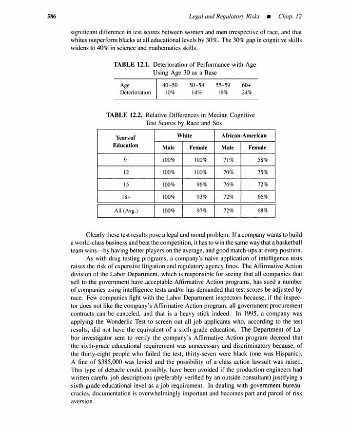
586 Legal and Regulatory Risks • Chap. 12
significant difference in test scores between women and men irrespective of race, and thatwhites outperform blacks at all educational levels by 30%. The 30% gap in cognitive skillswidens to 40% in science and mathematics skills.
TABLE 12.1. Deterioration of Performance with AgeUsing Age 30 as a Base
AgeDeterioration
40-5010%
50-5414%
55-5919%
60+24%
TABLE 12.2. Relative Differences in Median CognitiveTest Scores by Race and Sex
Years of White African-American
Education Male Female Male Female
9 100% 100% 71% 58%
12 100% 100% 70% 75%
15 100% 96% 76% 72%
18+ 100% 93% 72% 66%
All (Avg.) 100% I 97% I 72% I 68% I
Clearly these test results pose a legal and moral problem. If a company wants to builda world-class business and beat the competition, it has to win the same way that a basketballteam wins-by having better players on the average, and good match-ups at every position.
As with drug testing programs, a company's naive application of intelligence testsraises the risk of expensive litigation and regulatory agency fines. The Affirmative Actiondivision of the Labor Department, which is responsible for seeing that all companies thatsell to the government have acceptable Affirmative Action programs, has sued a numberof companies using intelligence tests and/or has demanded that test scores be adjusted byrace. Few companies fight with the Labor Department inspectors because, if the inspec-tor does not like the company's Affirmative Action program, all government procurementcontracts can be canceled, and that is a heavy stick indeed. In 1995, a company wasapplying the Wonderlic Test to screen out all job applicants who, according to the testresults, did not have the equivalent of a sixth-grade education. The Department of La-bor investigator sent to verify the company's Affirmative Action program decreed thatthe sixth-grade educational requirement was unnecessary and discriminatory because, ofthe thirty-eight people who failed the test, thirty-seven were black (one was Hispanic).A fine of $385,000 was levied and the possibility of a class action lawsuit was raised.This type of debacle could, possibly, have been avoided if the production engineers hadwritten careful job descriptions (preferably verified by an outside consultant) justifying asixth-grade educational level as a job requirement. In dealing with government bureau-cracies, documentation is overwhelmingly important and becomes part and parcel of riskaversion.
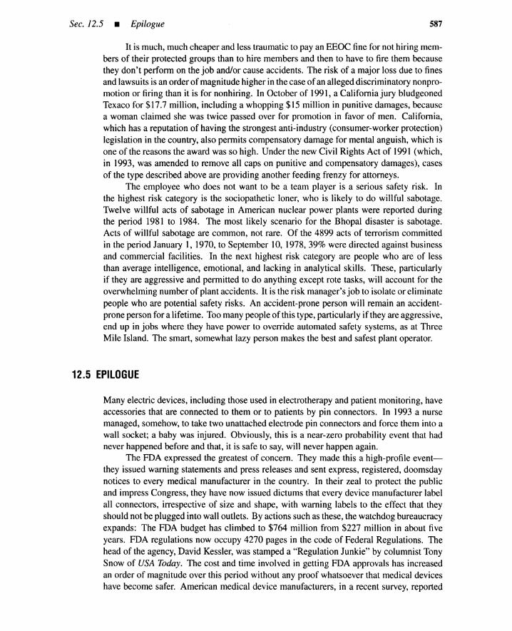
Sec. 12.5 • Epilogue 587
It is much, much cheaper and less traumatic to pay an EEOC fine for not hiring mem-bers of their protected groups than to hire members and then to have to fire them becausethey don't perform on the job and/or cause accidents. The risk of a major loss due to finesand lawsuits is an order of magnitude higher in the case of an alleged discriminatory nonpro-motion or firing than it is for nonhiring. In October of 1991, a California jury bludgeonedTexaco for $17.7 million, including a whopping $15 million in punitive damages, becausea woman claimed she was twice passed over for promotion in favor of men. California,which has a reputation of having the strongest anti-industry (consumer-worker protection)legislation in the country, also permits compensatory damage for mental anguish, which isone of the reasons the award was so high. Under the new Civil Rights Act of 1991 (which,in 1993, was amended to remove all caps on punitive and compensatory damages), casesof the type described above are providing another feeding frenzy for attorneys.
The employee who does not want to be a team player is a serious safety risk. Inthe highest risk category is the sociopathetic loner, who is likely to do willful sabotage.Twelve willful acts of sabotage in American nuclear power plants were reported duringthe period 1981 to 1984. The most likely scenario for the Bhopal disaster is sabotage.Acts of willful sabotage are common, not rare. Of the 4899 acts of terrorism committedin the period January 1, 1970, to September 10, 1978,39% were directed against businessand commercial facilities. In the next highest risk category are people who are of lessthan average intelligence, emotional, and lacking in analytical skills. These, particularlyif they are aggressive and permitted to do anything except rote tasks, will account for theoverwhelming number of plant accidents. It is the risk manager's job to isolate or eliminatepeople who are potential safety risks. An accident-prone person will remain an accident-prone person for a lifetime. Too many people of this type, particularly if they are aggressive,end up in jobs where they have power to override automated safety systems, as at ThreeMile Island. The smart, somewhat lazy person makes the best and safest plant operator.
12.5 EPILOGUE
Many electric devices, including those used in electrotherapy and patient monitoring, haveaccessories that are connected to them or to patients by pin connectors. In 1993 a nursemanaged, somehow, to take two unattached electrode pin connectors and force them into awall socket; a baby was injured. Obviously, this is a near-zero probability event that hadnever happened before and that, it is safe to say, will never happen again.
The FDA expressed the greatest of concern. They made this a high-profile event-they issued warning statements and press releases and sent express, registered, doomsdaynotices to every medical manufacturer in the country. In their zeal to protect the publicand impress Congress, they have now issued dictums that every device manufacturer labelall connectors, irrespective of size and shape, with warning labels to the effect that theyshould not be plugged into wall outlets. By actions such as these, the watchdog bureaucracyexpands: The FDA budget has climbed to $764 million from $227 million in about fiveyears. FDA regulations now occupy 4270 pages in the code of Federal Regulations. Thehead of the agency, David Kessler, was stamped a "Regulation Junkie" by columnist TonySnow of USA Today. The cost and time involved in getting FDA approvals has increasedan order of magnitude over this period without any proof whatsoever that medical deviceshave become safer. American medical device manufacturers, in a recent survey, reported
588 Legal and Regulatory Risks • Chap. 12
overwhelmingly that the FDA was hindering the introduction of new and improved medicaldevices, and that their R&D programs have been curtailed. Most large medical-devicecompanies, such as Baxter, have had major layoffs; others, such as Johnson & Johnson andBristol-Meyers Squibb, have spun off their device divisions. William George, president ofMedtronics, recently testified before Congress that he is moving a major research laboratoryto Europe because of legal and regulatory problems in the United States. Many engineeringjobs have been lost.
One sees this across the entire industrial sector. The chemical industry has curtailedR&D and the number of new chemicals put on the market has been drastically reduced. Thelatest EPA pronouncements on the dangers posed by chlorine and all chlorine-containingchemicals has paralyzed entire segments of the industry. Certainly, projected plant expan-sions have been canceled.
If one accepts the notion that many of the regulatory actions, such as the one mandatingfarm-product-based gasoline additives, are politically motivated, then they can only becountered by political action. It is quite clear that industry and industry associations donot have enough clout to defend themselves, nor do they have a political constituency thatcontrols votes.
It is suggested that the engineering and scientific societies do what health profes-sionals, lawyers, and others did decades ago: form political action committees. Politicalaction is not un-American nor is it enlightened self-interest. There are about 1.5 millionscientists and engineers in this country: if organized, they could make a difference. Thereis nothing un-American about engineering organizations demanding that OSHA and FDAfactory inspectors be registered engineers. There is nothing un-American about the sci-entific societies asking that directors of agencies such as the EPA come from a scientific,rather than a legal/political, arena. It would appear that, at present, anyone who has everworked in industry is automatically disqualified from working for a regulatory agency. Thereverse should be the case.
In a recent lecture at the University of Delaware, one of the authors (E. J. Henley)distributed a questionnaire to the students asking if they favored their professional societiesuniting and forming political action committees; the response was overwhelmingly "yes."The same affirmative response was given by a group of working chemical engineers thatwas posed the same question. Industries can be sued and regulated to death; the livingproof is the nuclear industry, which has moved ahead in most countries and is moribundin America, due largely to the staggering burden posed by lawsuits and regulatory actions.Perhaps nuclear power, in the long run, will prove economically nonviable, but we willnever know unless the assessment is made by engineers and scientists instead of politicians,regulators, and activist lawyers.

ndex
A
Age, 332A posteriori distribution, 142
of defect, 32of frequency, 32of reliability, 353
A priori distribution, 142of defect, 31of frequency, 32of reliability, 353uniform, 352
Abnormally long failure times, 348AC power recovery, early or late, 150,
157-58Accident management, 79,84
critique of, 84Accident mechanisms, 55-75Accident prevention, 78-9Accident progression groups, 103, 159Accident sequence, 14, 16, 100,246
cutset, 153-54,246-51expression of, 154grouping of, 103, 117, 126, 156quantification of, 117, 124, 155screening of, 117, 124
Accident sequence for blackout, 152AFWS heat removal, 149ALARA, seeAs low as reasonably
achievableAlarm function, 416-20
FD function, 418FD probability, 419
FS function, 416FS probability, 419
Alternatives, 8-9, 22cost of, 12for life-saving, 12for rain hazard mitigation, 9risk-free, 10
Ammonia storage facility, 97Analysis
accident frequency, 103, 117,148-56
accident progression, 103, 126,156-59
common-cause failure, 240, 446-69consequence, 103, 127, 162-63database, 117, 125,539-41dependent failure, 117, 124, 425-70deterministic, 102event tree, 14, 70
fault tree, 98, 165-226human reliability, 117, 125,
471-534initiating event, 117-18Laplace transform, 299-302~arkov,427-45,467-69
plant familiarization, 117preliminary forward, 176preliminary hazard, 104-8risk-cost, 12, 24risk-cost-benefit, 12, 25sensitivity, 13, 525source-term, 103, 127, 159-62
task,503THERP sensitivity, 525uncertainty, 117, 126, 156, 535-72
AND causal propagation, 21Anticipated disturbances, 79Aperture, equipment or flow, 197, 199Aperture controller
analog flow controller (AFC), 202closed to open equipment (COE),
199with command, 199without command, 199digital flow controller (DFC), 202normally closed equipment (NCE),
199normally open equipment (NOE),
199open to close equipment (OCE), 202
Aperture controller gain, 201-2APET, seeEvent treeAs low as reasonably achievable, 40
versus de minimis, 41Attitudes
risk-aversive, 31-2risk-neutral, 28
risk-seeking, 28Attitudes for monetary outcome, 27Attitudes, inattentive, 71Automatic actuation, 83Availability, 35, 272, 281, 287, 363
component, 272, 281system, 363
589

590
B
Backward approaches, 175Barriers, I I, 56, 82
horizontal or vertical, 81Basic event or failure, 59, 165, 172Basic event OR gates, 237Basic event quantification,263-337
combined process, 271-74, 280-85failure-to-repairprocess, 278-80flowchart of, 288, 290repair-to-failureprocess, 265-71,
274-78Basic human error probability,504,
530-33assignment example, 514
Basic-parameter model, 456-61Bayes formula, single- or two-stage,
539Bayes theorem
for continuous variables, 143, 352for discrete variables, 142, 351
Bayesianexplanationof likelihood overestimation,32of severity overestimation,31
Benefits,25Beta-distribution, 307, 544Beta-factor model, 449-56
component-levelanalysis, 455train-levelanalysis, 453
BHEP,see Basic human errorprobability
Bias and dependenceamong components, 548among experts, 547
Binomialdistribution,48, 306, 331,349-51,368
Binomial data propagation, 552Binomial failure-rate model, 464-67Booleanexpression, 123Boolean manipulationrules, 143-44,
147-48absorption laws, 148, 248associative laws, 148commutative laws, 148complementation, 148, 248de Morgan's laws, 148,366distributive laws, 148idempotent laws, 148, 248merging, 254operations with 0 and 1, 148reduction, 254
Boolean modules, 255-57Boolean variable and Venn diagram,
144, 146Boundaryconditions
at equipment nodes, 203at flow nodes, 202
Breakevenpoint, 13
cCancer probability,21Causal scenario, 14Cause consequence diagram, 45Causes, see Events. See also Failures
direct, 60indirect, 60main, 60root, 60supplemental, 60
Certification, 87, 91Change control, 80Checklist, 88, 105, 110X2-distribution, 346-47, 351,
355-56Common-causecut sets, 240, 242Common-cause failure, 426Common-cause failure analysis,
446-69component-levelanalysis, 455failure on demand, 446, 458, 464feedwater system, 453, 455one-out-of-three pump system, 460,
466run failure, 446, 460,466subcomponent-level analysis,
446-48system configurations,446train-levelanalysis, 453two-out-of-threevalve system, 458,
464Common causes
and basic events, 241categories, 242examples, 242floor plan, 243location of basic events, 243sources, 242
Communication, 71Component
interrelations, 175variety,57
Component parametersavailability, 272, 281, 287conditional failure intensity,282,
287conditional repair intensity,283,
287definitionsummary,336expected number of failures, 273,
282,287expected number of repairs, 273,
284,287failure density, 268, 275, 286failure rate, 268, 275, 286histogram, 265, 267mean residual time to failure, 277mean time between failures, 284,
287
Index
mean time between repairs, 285,287
mean time to failure, 276, 286mean time to repair, 279,286reliability,265, 274, 286repair density, 279, 286repair distribution, 278, 286repair rate, 279, 286stationary values, 287, 298, 30 Isummary of constant rate models,
298time to failure, 276time to repair, 279unavailability, 273, 281, 287unconditionalfailure intensity,273,
282,287unconditional repair intensity,273,
284,287unreliability, 265, 275, 286
Concept design, 87-8Conditional failure intensity,282, 287,
364Conditional probabilities, 138-43
alternativeexpression of, 140bridge rule, 141chain rule, 139definitionof, 138independence in terms of, 140simplificationof, 146
Conditional repair intensity,283, 287Confidence intervals, 339-62
Bayesianapproach, 351-54classical approach, 340-51of failure rate, 348general principles, 340-46of human error, 543of mean time to failure, 346of population mean, 343-45of population variance,346of reliability,348, 350-52
Confusion matrix approach, 509-11Consequence, 57, 103, 130Consequence mitigation,78-9, 84Constant-failureand repair rates,
297-304,332behavior of, 393combined process, 299-302failure-to-repair process, 299Laplace transform analysis,
299-302Markovanalysis, 303repair-to-failureprocess, 297-99summary of constant rate models,
298Constant failure rate, 286Constant repair rate, 286Containment failure, 79, 157-58Control systems, 82Convexcurve, 27

Index
Countermeasures, onsite or offsite, 56Coupling mechanisms
common unit, 73functional, 72human, 73proximity, 73
Coverage formula, 389Cut sets, 227
categories of, 240common-cause, 240covariance of, 569effects of, 156equation, 155minimal, 229
D
Damage, 46, 56Decision tree, 122Departure monitor, 97Dependency
by common loads, 426by common-unit, 425explicit, 124functional, 425implicit, 124intersystem, 425intrasystem, 425by mutually exclusive events, 426by standby redundancy, 426subtle, 426
Dependency assessment, 504complete dependence (CD), 504example of, 520high-level dependence (HD), 504low-level dependence (LD), 504moderate-level dependence (MD),
504zero dependence (ZD), 504
Dependent failure, 68by management deficiencies, 72, 75quantification process, 425-70
Design review, 87Design weakness, 88Detail design, 87-8Detection-diagnosis-response, 473Determinism and indeterminism, 478Diagnosis, 20, 473, 508, 525Diesel generators, 148Discrete probability algebra, 564-66Distribution parameters
kurtosis, 561mean, 328median, 328mode, 328moment, 329skewness, 561standard deviation, 328variance, 328
Distribution pointsex points, 340median-rank plotting position, 334percentage points, 340percentile, 340
Distributionsbeta, 307, 544binomial, 48, 306, 331, 349-51, 368X2,346-47,351,355-56
exponential, 305, 329Fisher F, 346, 348, 357-59gamma, 307, 332graphs of typical distributions, 308Gumbel, 306inverse-Gaussian, 307log-normal, 305, 320-22, 330,
541-49multinomial, 331, 350normal, 305, 330Poisson, 306, 331Poisson approximation, 332Studentt, 344-45, 356-57summary of typical distributions,
305-7Weibull, 305, 311-18, 330
Distributions, continuous or discrete,327-28
Dose, individual or collective, 21
E
Equal probability intervals, 565Equipment library, 199
aperture controller, 199generation rate controller, 202
Equity value, 25Ergodic theorem, 319Errors
accident-procedure, 125cognitive, 20, 61commission, 61intentional, 67lapse, 61mistake, 61omission, 61pre-initiator, 125recovery, 125routine, 61slip,61
ET, see Event treeEvacuation timing, 161Event development rules, 204
acquisition of, 206examples of, 205for new equipment, 218types of, 204
Event layer, 67Event symbols, 172
circle, 172
591
diamond, 172house, 174oval, 173rectangle, 172triangle, 174
Event tree (ET)accident progression ET (APET),
126construction of, 117, 119coupled with fault tree, 119function ET, 119heading analysis of, 154pruning of, 100system ET, 119
Event tree analysis, 14, 70Event tree for
operators and safety systems, 71pipe-break, 99, 101
pressure tank system, 16, 195reactor plant, 182, 191single track railway, 97station blackout, 150support system, 121swimming pool reactor, 214
Event-likelihood model, 68Events
anticipated abnormal, 63, 79complex, below design basis, 63, 79complex, beyond design basis, 63,
79enabling, 61
equipment failure, 205equipment-suspected, 204external, 61, 69house, 208initiating, 61, 95,103internal, 61LOCA,62repeated, 240state of component, 184transient, 62
Excessive specialization, 81Expected cost, 378Expected number of failures, 273,
282,287,364
Expected number of repairs, 273, 284,287
Expected utility, 13, 27Expert opinion, 20, 33, 539-40Experts and public, 32-4Experts integration of PSFs, 492Exponential distribution, 305, 329External PSFs
job and task instruction, 487situational characteristics, 485stressors, 487task and equipment characteristics,
485

592
F
FAFR,8Fail-safedesign, 83Fail-soft design, 83Failed-dangerousfailure, 66Failed-safe failure, 65Failure data for
bearing, 31Icomponent failure rates, 538guidance system, 311, 314human life, 266reformer tubes, 316transistors, 277
Failure density, 268, 275, 286, 364Failure mode, 109
application factor, 112criticality number, 112-13effect probability, 112environmental factor, I 12generic, )09ratio, 112
Failure prevention,78, 165for device, 80for human error, 80for individual, 80for organization, 81for teams, 81
Failure rate, 68, 112,268, 275, 286age-dependent,415
Failuresactive, 60, 62basic,59, 165cascade, 60chronological distribution of, 62command, 59, 179common-cause, 74common mode, 74demand,60dependent, 61design, 62early, 271functional, 59hardware-induced,60human-induced,60independent,6)initial, 60interface, 59intermediate,59intermittent,60latent, 60manufacturingand construction, 62mechanical,59operation, 62parallel,60passive,62persistent, 60primary,59, )79
propagating,75random, 60, 271recovery,61run, 60secondary,59, )79siting, 62support system, 108system-induced,60validation,62wearout, 60, 271
Farmer curves, 4Fatality,early or chronic, 39, 129, 161FATRAM, 237-39Fault tree
alternative representationof, 47as AND/OR tree, 124building blocks, 166with event tree, 16without event tree, 186multistate, 257noncoherent, 251-58, 260structure of, 166structured programmingformat of,
180value of, 166
Fault-treeanalysis (FTA),98, 165-226Fault-treeconstruction, 165-226
automated, 196-222boundary conditions, 210, 214, 220downwardevent development,207event development rules, 204heuristic guidelines for, 184heuristic procedure for, 179-96recursive three-value procedure for,
206upward truth propagation,207
Fault-treeconstruction exampleschemica) reactor, 215relay circuit, 210swimming pool reactor, 211, 248
Fault tree forAFWS failure, 153automated shutdown failure, )92automated/manualshutdown
failure, 194component failure, 186domestic hot-water system, 259emergencyac power failure, 153excess feed, 192excessivecurrent in circuit, 173excessivecurrent to fuse, 182, 184fire, 168lack of low-levelsignal, 216lack of trip signal, 216manual shutdown failure, 193motor failure to start, )8)motor to overheat, 47
Index
open aperture, 221operator failure to shutdown, 169partial loss of power, 171piston 3 drop, 216piston 4 drop, 216positive flow rate, 216-17power unavailable, 170pressure tank rupture, 16, 187-88,
195,228pump overrun, 196relay system failure, 261tail-gas quench and clean-up, 371,
438temperature increase, 221unnecessaryshutdown, 171, 174zero flowrate, 211, 221
Fault-tree linking, 246-51Fault-tree module
examples of, 215, 220, 234-35hierarchy of, 217identificationof, 208, 257repeated and/or solid modules, 210simple, 234sophisticated,234
Fault-treesimplification,243, 245Fault-tree truncation, 206Feed and bleed operation, 525Fisher F distribution, 346, 348,
357-59Fission product release criteria, 44Row node recurrence, 208Row rate, 197Flow triple event, 198Rows, 197FMECA,89,110FMEA,89, 104, 108
criticality, 110severity, 110
Forwardapproaches, I75FTAP, 236FTA,see Fault-treeanalysis
G
Gamma distribution, 307, 332Garden path, 473Gates
AND,166conditions induced by, 188exclusive OR, )69inhibit, )67m -out -of-n, 168OR, 166priority AND, 169voting, 170
General failure and repair rates, 304Generalized consensus, 254, 258Generation rate, 197

Index
Generation rate controllerbranch, 202flow sensor, 202junction, 202logic gates, 202pressure sensor, 202temperature sensor, 202
Generic plant data, 538-39Geometric average, 538Goals, see Safety goalsGumbel distribution, 306
H
Hamlet, 473Hardware failures, 69, 263-337
early or initial, 271, 331human-induced, 69random, 69, 271, 331wearout, 271, 310, 331
Hazard and operability study, 104, 113versus FMEA, 114guide words, 113process parameter deviations, 114
Hazardous energy sources, 105Hazardous process and events, 105Hazards ranking scheme, 106HAZOPS, see Hazard and operability
studyHeR, see Human cognitive reliabilityHEP, see Human error probabilityHiring process, 584HRA, see Human reliability analysisHRA event tree, 500HRA event-tree development, 503HRA event tree for
calibration task, 500control room actions, 523-24, 526operator outside control room, 518
Human abilitylife-support, 475manipulative, 475memorizing, 475sensing, 475thinking, 475
Human and machine, 474Human as computer, 474-81Human cognitive factors
knowledge-based factors, 484rule-based factors, 484skill-based factors, 484
Human cognitive reliability, 506-8,525-30
correlation parameters, 507model curves, 507normalized time, 507
Human cognitive reliability forloss of feedwater, 525manual plant shutdown, 508
Human during panic, 480-81Human error bounds, 543-44Human error examples
of lapse/slip type, 497-98of thought process, 494-97
Human error probability, 490-92,501,506
assignment, 503Human error probability tables,
530-33administrative control failure, 532check-reading displays, 532manual control operation, 532omission in written procedures, 530quantitative-reading displays, 530recalling oral instructions, 533responding to annunciator, 533valve change, 531
Human error screening valuesfor nonresponse and wrong actions,
492for test and maintenance, 491
Human errors, 69active, 69classification of, 472lapse/slip (commission), 474lapse/slip (omission), 474latent, 69misdiagnosis, 474mistake, 474nonresponse, 474recovery, 69
Human hardware factorspathological, 481pharmaceutical, 481physical, 481physiological, 481six P's, 484
Human performance phasesactive, 479panic, 479passive, 479unconscious, 479vacant, 479
Human performance variations,478-81
Human psychological factors, 481Human reliability analysis, 471-534Human reliability fault tree, 528Human task attributes
communication, 487complexity, 486continuity, 487criticality, 486feedback,486frequency and repetitiveness, 486narrowness, 486
Human weakness, 26alternation, 477
593
bounded rationality, 478cheating and lying, 478dependence, 478frequency bias, 478gross discrimination, 478imperfect rationality, 478incomplete/incorrect knowledge,
478naivety, 478perseverance, 477queuing and escape, 478reluctant rationality, 478shortcut, 477similarity bias, 478task fixation, 477
Human-machine interface, 487
Inclusion-exclusion formula, 387-89,427,438
bracketing procedure, 407inner bracket, 407outer bracket, 407second correction term, 406for system failure intensity, 404-9for system unavailability, 388,402two-out -of-three system, 388
Incomplete beta function, 335Independence, outer or inner, 82Independent basic events, 365Individual risk, 15Information matrix, 568Information, excessive or too little, 67Initiating event, 15
grouping of, 119search for, 104
Insurance premium, 27-8Interactions
negative, 57taxonomy of, 58-62
Internal PSFscognitive factors, 484hardware factors, 481psychological factors, 481
Inverse-Gaussian distribution, 307Isolation failure, 250
K
KITT, 391-415minimal cut-set parameters,
397-402summary of parameters, 392system failure intensity, 404-10system unavailability, 402-4
KITT computationsequations for, 395flow sheet of, 394

594
KITT computations forinhibit gate, 414minimalcut-set parameters, 397single-componentsystem, 394three-componentseries system, 397two-componentparallel system,
400,403two-componentseries system, 402,
405two-out-of-threesystem, 400, 403,
408,410,412Knowledge-based behavior,488
L
Labeling, 90Labor force problem, 583Laplace transform, 299
convolution integral, 300inverse transform, 300
Large ETIsmaIl FT approach, 120Latin hypercube sampling, 553Lawsuits
by governmentagencies, 576nonproduct,575product liability,575risk mitigation,578
Leg~risk~573-88
Level I PRA, 117-26risk profile, 130
Level 2 PRA, 126risk profile, 130
Level 3 PRA, 127examples of, 132risk profile, 128for station blackout, 148-63
Life testsfailure-terminated, 346, 567time-terminated,346, 567
Lifetime data propagation,553Likelihood, I, 19
annual, 39objective, 2subjective, 2, 21
Likelihood layer, 67, 71Log-normaldistribution, 305, 320-22,
330,541-49Log-normaldetermination, 542Log-normal summary,542Logic, backward or forward, 100Loss
downtime, 47expected,47full or half, 378
Loss functionrisk-aversive, 28risk-neutral, 28risk-seeking, 28
Loss or gain classification,22Lotteries, I0, 28, 80
M
Maintenance, 72Managementdeficiencies,72Manual example, 513Markov analysis, 427-45, 467-69
differential equations, 429-30,437,439,468
Laplace transform analysis, 431transition diagram, 303, 429-30,
436-37,440,445,469Master logic diagram, 104, 115-16MAUD,492Maximum-likelihoodestimator,
567-69for beta factor, 451for mean time to failure, 347
Mean residual time to failure, 277Mean time between failures, 284,287Mean time between repairs, 285, 287Mean time to failure, 276, 286, 365Mean time to repair, 279, 286Mental process types
determination of, 488knowledge-basedbehavior,488nonroutine task, 488routine task, 488rule-based behavior,488skill-based behavior,488
MICSUP, 231Minimal cut set, 229Minimal cut-set generation, 231
Boolean manipulationof, 231bottom-up, 231for large fault trees, 234for noncoherent fault trees, 251-58,
260top-down, 229
Minimal cut-set subfamily,236Minimal path set, 229Minimal path set generation
bottom-up, 233top-down, 232
MLD, see Master logic diagramMOCUS, 229, 232MOCUS improvement,237Moment propagation,555-64
AND gate, 555ANDIOR gates, 557OR gate, 556by orthogonal expansion, 561by sum of minimalcut sets, 558by Taylor series expansion, 560
Monitor and control, 76Monte Carlo approach, 550-55
Index
MORT, IIMortalitydata, 266Multinomialdistribution, 331, 350MultipleGreek letter model, 461-64
N
Nelson algorithm, 253, 257Noncoherentfault trees, 251, 260Normal distribution, 305, 330Nuclear reactor schematic
diagram of, 64shutdown system of, 64
NUREG-1150, 102
oOAT, see Operator action treeOccurrence density, 3Operation, 72
emergency,214, 218normal, 213, 215
Operator action tree (OAT), 473Operator examples, 14, 16, 191,
471-534OR causal propagation,21Orthogonal polynomials, 569-71Outcome, I
chain termination, 19guaranteed, 4incommensurabilityof, 23localized,5realized,6
Outcome matrix, 10Outcome significance, 12, 22Overestimation
of outcome likelihood, 31of outcome severity,31
Overregulation,582
p
Panic characteristics, 480-81Parameterestimation
for command failures, 325for constant failure rate, 309for failure-to-repairprocess, 318-22for human errors, 326for log-normal parameters,320-22for multiple failure modes, 322for repair-to-failureprocess, 309-18for secondary failures, 325for system dependent basic event,
327for Weibull parameters, 311-18
Parameterestimation situationall samples fail, 309early failure data, 311incomplete failure data, 309, 334wearout, 316

Index
Pareto curve, 24Parts and material (P/M) assurance, 89Pass-fail propagation, 552Path sets, 227
minimal, 229Performance shaping factors, 481-89
evaluation of, 504example of, 519external PSFs, 484importance of, 493internal PSFs, 481rating of, 493
PHA, see Preliminary hazard analysisPhysical containment, 55-6Pilot production, 87Plant
boundary conditions, 176with hazardous materials, 97without hazardous materials, 96,
130initial conditions, 176
Plant specific data, 539Poisson distribution, 306, 331Population
affected, 15, 19risk, 15, 48-52size effect, 17, 48-52
PORV stuck open, 157Post-design process, 87PRA, see Probabilistic risk assessmentPRAM, see Risk management. See
also Probabilistic riskassessment
PRAM credibility problem, 35Preliminary hazard analysis, 104-8Preproduction design process, 86-93Pressure tank rupture PRA, 14-5Probabilistic risk assessment (PRA),
6,95-164benefits, detriments, success of,
132-36differences in, 18five steps for, 103with modifications, 102for nuclear power plant, 98source of debates, 18three levels of, 117
Probability, see Conditionalprobabil ities
Probability and Venn diagram, 145Probability density, 327Procedure-following errors, 499-506Procedures
maintenance, 72operation, 72symptom-based, 83
Product of log-normal variables, 545Propagation prevention, 79, 81, 165
Propagationscascade, 58parallel, 58, 74series, 58, 74of uncertainty, 549-66
Prototype production, 87Proven engineering practice, 76-7PSF, see Performance shaping factorsPublic confidence, 31
Q
Quality assurance, 76-7Quality assurance program, 85-6Quality control, 77Quality monitoring, 91Quantification of
basic events, 263-337dependent events, 425-70system, 363-423
Quantitative design objectives(QDOs),35-52
cancer fatality, 43cost-benefit guideline, 43general performance, 43plant performance, 43prompt fatality, 43
R
Radionuclide classes, 159Railway
collision, 97freight, 97passenger, 96
Rain hazard mitigation problem, 9Reactor and turbine trip, 148Reactor coolant system (ReS)
integrity, 156pressure at UTAF or VB, 157
Reactor Safety Study (WASH-1400),4,98-100
Reactor trip, 214Recovery, 473Recovery actions, 494
neglect of, 503Recovery assessment example, 522Recovery of feedwater, 525Regulations and safety, 580Regulatory
agency fines, 579cutoff level, 49decisions, 5 Iresponse, 17risks, 573-88
Relations among parameterscombined process, 290-96common-cause analyses, 462failure-to-repair process, 289-90repair-to-failure process, 285-89
595
Releasemagnitude, 130probability, 101
Release fractions, early or late, 159Reliability, 35,265,274,286,364,
444component, 265, 274, 286cut-set or system, 364, 415
Reliability assessment, 89Reliability block diagram, 123
versus fault tree, 373Reliability block diagram for
chemical reactor, 260pressure-tank rupture, 228tail-gas quench and clean-up
system, 371Renewal process, 292Repair crew size, 439Repair data for electric motors, 280Repair density, 279, 286Repair distribution, 278, 286Repair rate, 279, 286Repairability, 444Response time
actual median, 492nominal median, 492for shutdown failure detection, 508,
525Response/action, 473Risk
acceptable, 48accumulation problems, 40assessment, 6common features of plants, 55-7controllability, 8-9daily, 8de minimis, 41definition of, 1-18different viewpoints of, 18individual, 15, 17, 43management of, 6population, 15, 17,43primitives of, 18technological, 33-4
Risk and safety, 36Risk aversion, 26-35
goals, 44mechanisms for, 31
Risk calculation, 103Risk curve uncertainty, 535Risk homeostasis, 24, 26Risk management, 7, 75-85
differences in, 22principles, 75
Risk management process, 79Risk neutral line, 48Risk profile, 2, 95, 103
by cause consequence diagram, 45complementary cumulative, 4

596
Risk profile tcont.)
significanceof, 22uncertaintyof, 131
Routine errors, 499-506Routine production, 87Rule-based behavior,488
sSafety, 36Safety culture, 76, 584Safety goals, 35-52
algorithmic frameworkfor, 38for catastrophic accidents, 43constant fatality model for, 50constant likelihood model for, 50decision structure of, 37geometric mean model for, 50hierarchical, 36idealistic, 48necessity versus sufficiencyof, 49for normal activities, 42of plant performance,71pragmatic, 48for prescreening,38quantitativedesign objectives
(QDOs),43regulatorycutoff level of, 49upper and lower bound of, 37, 42-3
Safety knowledge,71Safety margins, 80Safety system
expenditure, 23malfunctions,64one-time activation,67operating range, 65trip actions, 65unavailability, 70
Sample mean, 341SAMPLE program, 551, 563Sample variance, 344Secondary event or failure, 59, 172,
179Secondary loop pressure relief, 149Semantic network, 197
construction, 202module flow nodes, 208repeated moduIe nodes, 209representation,202solid-module nodes, 209
Semantic network forchemical reactor, 219relay system, 202swimming pool reactor, 213
Sensordiversion, 67failure, 67incorrect location, 66secondary informationsensing, 67
Sensor systemscoherent three-sensor systems, 4 I7demand probability,419failed-dangerousfailure, 418failed-safe failure, 416parallel system, 416series system, 416, 418three-sensor system, 420too many alarms, 67two-out-of-three system, 4 I6two-sensor system, 419
SETS, 236SHARP,498-99Shock, lethal or nonlethal,464-65Short-cut calculation, 410-13
for component parameters,410for cut-set parameters,410for system parameters,412
Shutdown, automated or manual, 191Significance, 12
fatality outcome, 30marginal, 29
Simplificationbyvery high probability, 183very low probability, 183
Simulated validation,67Singleton, 255Skill-based behavior,488SLIM, 492SLIM PSFs
complexity,493consequences, 493process diagnosis, 493stress level, 493team work, 493time pressure, 493
Small ET/large FT approach, 122Small group activities, 77Software quality assurance (SQA), 90Source term groups, 103, 160Spare pump, 377Specificationand its changes, 86Stabilization of unsafe phenomena,56Standardization, 80Standby redundancy, 427-45
cold standby,427, 432, 441failures per unit time, 442hot standby,427, 433, 441m-component redundancy, 439-42reliability,444repairability,444steady-state unavailability, 439-42tail-gas system unavailability, 433three-component redundancy,
434-39transition diagram, 429-30,
436-37,440two-component redundancy,
428-34warm standby,427,430,441
Index
Station blackout, 148-63Steam generator
heat removal from, 157tube rupture of, 157
Stimulus-organism-response, 473Stratifiedgrouping, 161Stress levels and human error
error probability and bounds, 49 Iunder extremely high stress level,
490under moderatelyhigh stress level,
490under optimal stress level, 490under very low stress level, 489for wrong control selection, 490
Structure function, 379alarm function, 4 I6-20coherent, 390minimalcut representation,383minimalcut structure, 383minimal path representation, 384minimal path structure, 385partial pivotaldecomposition, 386unavailabilitycalculations, 380
Structure function for, 379-83AND gate, 379bridged circuit, 382OR gate, 379tail-gas quench and clean-up,
380-81two-out-of-threesystem, 380-81,
384,386-87Student t distribution, 344-45, 356-57Subjectiveestimates, 20Success likelihood index (SLI), 492Success tree, 372Superset examinations, 237, 239Survivaldistribution, 267Symmetry assumption, 457System parameters
availability, 363conditional failure intensity,364expected number of top events, 364failure density, 364mean time to failure, 365reliability,364, 444repairability,444unavailability, 363unconditionalfailure intensity,364,
442-44unreliability, 364
System unavailabilityAND gate, 365combination of gates, 369m-out-of-n system, 367-69OR gate, 365parallel system, 373series system, 373tail-gas quench and clean-up, 370voting gate, 367-69

Index
System unavailability boundsEsary and Proschan bounds,
390,402inclusion-exclusion bounds,
389,402partial minimal cuts and paths, 390tail-gas quench and clean-up
system, 391two-out-of-three system, 389-90
Systemsautomobile braking, 224domestic hot water, 164, 224electrical circuit, 224-26emergency safety, 56engineered safety, 82four way stations, 223heaters, 225normal control, 56, 82topography of, 175
T
Task analysis, 503Task analysis example, 514Task requirements
anticipatory, 485calculational, 486decision-making, 486interpretation, 486motor, 485perceptual, 485
Testfor equal means, 345for equal variances, 346extensive, 91simulated, 91
THERP, 499-506, 513-25general procedure, 502
THERP examplescalibration task, 500errors during plant upset, 513-25test and maintenance, 505
THERP sensitivity analysis, 525Three-value logic, 207Time to failure, 276Time to repair, 279Timing consideration, 154Top event
finding, 175-79versus event tree heading, 186
Top event expressions, 211, 220, 250,448
Trade-offmonetary, 23-5, 28, 46risk/cost, 23risk/costibenefit(RCB), 25
Transition diagram forbasic-parameter model, 457beta-factor model, 449binomial failure-rate model, 465common-cause analysis, 468component states, 265m-component redundancy, 440multiple failure modes, 322primary and secondary failures, 326pumping system, 178three-component redundancy,
436-37two-component redundancy,
429-30Transition probabilities, 303Trip system failure, 249Truth table, 122Truth table approach to
AND gate, 374OR gate, 374pump-filter system, 375-78
Two-level computer configuration, 475
uUnavailability, 273, 281, 287, 363
component, 272, 281formula, 333population ensemble, 319system, 363time ensemble, 319
Uncertainty, 4, 103by data evaluation, 537by expert judgment, 538of failure rate, 68meta-,4modeling of, 536parametric, 536propagation of, 536, 549-66statistical, 536
597
Uncertainty propagation, 536, 549-66discrete probability algebra, 564-66moment propagation, 555-64Monte Carlo approach, 550-55
Unconditional failure intensity, 273,282,287,364,442-44
Unconditional repair intensity, 273,284,287
Unreliability, 265, 275, 286, 364Utility, 12
expected, 13, 23for monetary outcome, 30
vVagabond, 473Value function, 12, 18
risk-aversive, 28risk-neutral, 28risk-seeking, 28
Venn diagrams, 143-48, 189Verification, 78Vessel breach (VB)
containment pressure before, 157pressure rise at, 158ReS pressure at, 157size of hole, 157type of, 157water in reactor cavity at, 157
Visceral variation causesactivity versus rest rhythm, 479defense of life, 479instinct and emotion, 479
Voting logicone-out-of-two.G twice, 65two-out-of-four:G, 65
wWAMCUT,236WASH-1400,98Weather, good or bad, 129Weibull distribution, 305, 311-18, 330Weibull reliability for HCR, 506, 508,
527,529Word model, 176Workers compensation, 577Worst case avoidance, 27Wrong action, 509-11