Probabilistic Models for

Unsuper vised Learning

Zoubin GhahramaniSam Roweis

Gatsb y Computational Neuroscience UnitUniver sity Colleg e London

http://www.gatsby.ucl.ac.uk/

NIPS TutorialDecember 1999

Learning

Imagine a machine or organism that experiences over itslifetime a series of sensory inputs:����������������� ��������Super vised learning: The machine is also given desiredoutputs � ��� � ��������� , and its goal is to learn to produce thecorrect output given a new input.

Unsuper vised learning: The goal of the machine is tobuild representations from � that can be used forreasoning, decision making, predicting things,communicating etc.

Reinf orcement learning: The machine can alsoproduce actions � ��� � ��������� which affect the state of theworld, and receives rewards (or punishments) � � � � � ������� .Its goal is to learn to act in a way that maximises rewardsin the long term.

r

a

Goals of Unsuper vised Learning

To find useful representations of the data, for example:� finding clusters, e.g. k-means, ART� dimensionality reduction, e.g. PCA, Hebbianlearning, multidimensional scaling (MDS)� building topographic maps, e.g. elastic networks,Kohonen maps� finding the hidden causes or sources of the data� modeling the data density

We can quantify what we mean by “useful” later.

Uses of Unsuper vised Learning

� data compression� outlier detection� classification� make other learning tasks easier� a theory of human learning and perception

Probabilistic Models

� A probabilistic model of sensory inputs can:

– make optimal decisions under a given lossfunction

– make inferences about missing inputs

– generate predictions/fantasies/imagery

– communicate the data in an efficient way� Probabilistic modeling is equivalent to other views oflearning:

– information theoretic:finding compact representations of the data

– physical analogies: minimising free energy of acorresponding statistical mechanical system

Bayes rule

�— data set— models (or parameters)

The probability of a model given data set�

is:� � ��� �! � �"� � �#� � �� �"� �� �$� � �

is the evidence (or likelihood )� � �is the prior probability of� � ��� �

is the posterior probability of� �$� �! %&� �"� � �'� � �)(Under very weak and reasonable assumptions, Bayesrule is the only rational and consistent way to manipulateuncertainties/beliefs (Polya, Cox axioms, etc).

Bayes, MAP and ML

Bayesian Learning :Assumes a prior over the model parameters.Computesthe posterior distribution of the parameters: * +-,/.�0 1 .Maxim um a Posteriori(MAP) Learning :Assumes a prior over the model parameters * +2,31 .Finds a parameter setting thatmaximises the posterior: * +2,�.�0 1�4 * +-,51�* +"0 .6,51 .Maxim um Likelihood(ML) Learning :Does not assume a prior over the model parameters.Finds a parameter setting thatmaximises the likelihood of the data: * +"0 .7,51 .

Modeling Correlations

Y

Y 1

2

8 Consider a set of variables 9;:�<�=�=�=�<95> .8 A very simple model:means ?A@CB D29�@FE andcorrelations G @IH B D-9 @ 9 H EKJ D-9 @ E�D-9 H E8 This corresponds to fitting a Gaussian to the dataL M$NPO B Q6R�SCG QUTWVX�Y[Z]\ ^ J _R M`N J a O'b GcT : M$N J a O�d

8 There are e M e f _ Ohg R parameters in this model8 What if e is large?

Factor Anal ysis

YDY1 Y2

X1 KX

Λ

Linear generative model:ikj l mn�oPprq

j n stnvu w jx stn are independent y z2{r|�}�~ Gaussian factorsx w j are independent y z-{]|��j�j~ Gaussian noisex � � �

So, � is Gaussian with:� z`�P~l � z"��~ � z$�W����~��3�

ly z2{r| qKq�� u �&~

where q is a � � � matrix, and � is diagonal.

Dimensionality Reduction: Finds a low-dimensionalprojection of high dimensional data that captures most ofthe correlation structure of the data.

Factor Anal ysis: Notes

YDY1 Y2

X1 KX

Λ

� ML learning finds � and � given data� parameters (with correction from symmetries):� � � � � � �2� � ���� � � �2� � ����� no closed form solution for ML params� Bayesian treatment would integrate over all � and �and would find posterior on number of factors;however it is intractable.

Network Interpretations

YDY1 Y2

X1 KX

YDY1 Y2^^ ^

hidden units

output units

input units

encoder"recognition"

decoder"generation"

� autoencoder neural network� if trained to minimise MSE, then we get PCA� if MSE + output noise, we get PPCA� if MSE + output noises + reg. penalty, we get FA

Graphical Models

A directed acyclic graph (DAG) in which each nodecorresponds to a random variable.

x5

x3x1

x2

x4

� � � ¡ ¢ � �$£¥¤[¡#� �"£C¦¨§�£¥¤[¡� �$£ª©3§�£¥¤�«£)¦¬¡� �$£A­r§�£C¦¬¡#� �"£C®¨§�£ª©�«£¯­�¡Definitions: children, parents, descendents, ancestors

Key quantity: joint probability distribution over nodes.° �²±�£¥¤�«�£C¦�«�³�³�³C«´£ªµ�¶�¡P¢ ° �`� ¡(1) The graph specifies a factorization of this joint pdf:° �`� ¡K¢ · ° �"£ · §

pa( ¸5¹ ) ¡(2) Each node stores a conditional distribution over itsown value given the values of its parents.

(1) & (2) completely specify the joint pdf numerically.

Semantics: Given its parents, each node isconditionally independent from its non-descendents

(Also known as Bayesian Networks, Belief Networks,Probabilistic Independence Networks.)

Two Unkno wn Quantities

In general, two quantities in the graph may be unknown:º parameter values in the distributions » ¼"½ª¾À¿ pa( Á5 ) ú hidden (unobserved) variables not present in the data

Assume you knew one of these:º Known hidden variables, unknown parametersÄ this is complete data learning (decoupledproblems)

θ=?

θ=?

θ=?

θ=?

θ=?º Known parameters, unknown hidden variablesÄ this is called inference (often the crux)

?

?

??

But what if both were unknown simultaneously...

Learning with Hidden Variab les:

The EM Algorithm

X1

θ1

θ3θ2

θ4

XÅ

2 XÅ

3

YÆ

Assume a model parameterised by Ç with observablevariables È and hidden variables ÉGoal: maximise log likelihood of observables.Ê Ë Ç5Ì!Í ÎIÏÑÐ Ë È Ò7Ç5Ì!Í ÎÓÏ Ô Ð Ë ÈÖÕ�É Ò6Ç5Ì× E-step : first infer Ð Ë É ÒØÈÖÕÙÇÛÚÝÜßÞ�Ì , then× M-step : find Ç�àráãâ using complete data learning

The E-step requires solving the inference problem:finding explanations, É , for the data, Ègiven the current model Ç .

EM algorithm & -function

XÅ

1

θ1

θ3θ2

θ4

X2 X3

Y

Any distribution ä å$æ ç over the hidden variables defines alower bound on èIéÑê å`ë ì6í3ç called î å2ä ïÙí5ç :èÓécê å ë ì7í5ç ð èÓé ñ ê å$æ ï�ë ì7í5çòð èÓé ñ ä å$æ ç ê å$æ ï´ë ì7í5çä å$æ çó ñ ä å$æ ç]èÓé ê å$æ ï[ë ì6í5çä å$æ ç ð î å2ä ïÙí5çE-step: Maximise î w.r.t. ä with í fixedä ô�å$æ çòð ê å$æ ìØëÖïÙí5çM-step: Maximise î w.r.t. í with ä fixedírôõð ö ÷�øù ñ ä ôúå$æ çûèÓéÑê å$æ ï[ë ì6í3çNB: max of î å2ä ïÙí5ç is max of èÓéÑê å`ë ì6í5ç

Two Intuitions about EM

I. EM decouples the parameter s

XÅ

1

θ1

θ3θ2

θ4

X2 XÅ

3

Y

The E-step “fills in” values for the hidden vari-

ables. With no hidden variables, the likeli-

hood is a simpler function of the parameters.

The M-step for the parameters at each n-

ode can be computed independently, and de-

pends only on the values of the variables at

that node and its parents.

II. EM is coor dinate ascent in ü

EM for Factor Anal ysis

YDY1 Y2

X1 KX

Λ

ý þ2ÿ ������� ÿ þ���� ��� þ���������������� � ÿ þ����� �Ñÿ þ��������E-step: Maximise

ýw.r.t.

ÿwith

�fixedÿ �úþ���� � � þ������ �!����� " þ�#$� �!% � #$&'�

# � &'(õþ�&)&'( * +,�.-0/M-step: Maximise

ýw.r.t.

�with

ÿfixed:

1�2436587:9<;>=@?BADC - /EGF 7IHJ7LK 5M; - N 7OA�HQP$RTS�5M; - N 7OAQK 1�20=UP'=UVLK W

X The E-step reduces to computing the Gaussianposterior distribution over the hidden variables.X The M-step reduces to solving a weighted linearregression problem.

Inference in Graphical Models

W

X Y

Z

Singl y connected netsThe belief propagationalgorithm.

W

X Y

Z

Multipl y connected netsThe junction tree algorithm.

These are efficient ways of applying Bayes rule using theconditional independence relationships implied by thegraphical model.

How Factor Anal ysis is

Related to Other Models

Y Principal Components Anal ysis (PCA): Assumeno noise on the observations: Z [ \^] _ `ba c>dfe

Y Independent Components Anal ysis (ICA): Assumethe factors are non-Gaussian (and no noise).

Y Mixture of Gaussians : A single discrete-valuedfactor: g>h [ i and gDj [ k for all l m[ n .

Y Mixture of Factor Anal yser s: Assume the data hasseveral clusters, each of which is modeled by asingle factor analyser.

Y Linear Dynamical Systems : Time series model inwhich the factor at time o depends linearly on thefactor at time oqp i , with Gaussian noise.

A Generative Model for Generative Models

Gaussian

Factor Analysis (PCA)

Mixture of Factor Analyzers

Mixture of Gr

aussians (VQ)

Cs

ooperative Vt

ector Qu

uantization

Sv

BN, Boltzmann Machines

Factorial HMM

HMM

Mixture of

HMMs

Switching State-space

Models

ICALinear

Dynamical Sv

ystems (SSMs)

Mixture of LDSs

Nonlinear Dynamical Systems

Nonlinear Gaussian

Belief Nets

mix

mix

mix

switch

red-dim

red-dim

dyn

dyn

dyn

dyn

dyn

mix

distrib

hier

nonlinhier

nonlin

distrib

mix : mixture

red-dim : reduced dimension dyn : dynamics distrib : distributed representation

hier : hierarchical

nonlin : nonlinear

switch : switching

Mixture of Gaussians and K-Means

Goal: finding clusters in data.

To generate data from this model, assuming w clusters:

x Pick cluster y z {�|~}��T����}fw � with probability ���x Generate data according to a Gaussian withmean ��� and covariance �G�

� ���q� � ��T�q�

� ��� � y ��� ������� � y �

� ��T�q� � �6�

����� � � }!� � �

E-step : Compute responsibilities for each data vec.�'� ���

� � ��� � ��� � y ��� � ��� ��� ��� � ��� � ��� � ���O}��G� �� �� ��� � � � ��� � ��� � � � }�� � �

M-step : Estimate ��� , ��� and �G� using data weighted bythe responsibilities.

The k-means algorithm for clustering is a special case ofEM for mixture of Gaussians where � � �   ¡ ¢ £�¤ ¥§¦!¨

Mixture of Factor Anal yser s

Assumes the model has several clusters(indexed by a discrete hidden variable © ).Each cluster is modeled by a factor analyser:

ª «�¬q­q® ¯°²±q³

ª « © ® ´ ­�ª «�¬�µ © ® ´ ­

whereª «�¬�µ © ® ´ ­q® ¶ «¸· ° ¹»º ° º ° ¼ ½ ¾ ­

¿ it’s a way of fitting a mixture of Gaussiansto high-dimensional data

¿ clustering and dimensionality reduction

¿ Bayesian learning can infer a posterior over thenumber of clusters and their intrinsicdimensionalities.

Independent Components Anal ysis

YDY1 Y2

X1 KX

Λ

À Á Â�ÃÅÄÇÆ is non-Gaussian.

À Equivalently Á Â�ÃÅÄQÆ is Gaussian and

ÈÊÉ Ë ÌÄTÍ�Î�Ï É ÄÑÐ�Â�ÃÅÄÒÆÅÓ Ô Éwhere Ð�ÂÖÕMÆ is a nonlinearity.

À For × Ë Ø , and observation noise assumed to bezero, inference and learning are easy (standard ICA).Many extensions possible (e.g. with noise Ù IFA).

Hidden Markov Models/Linear Dynamical Systems

PSfrag replacements

ÚÜÛ

Ý Û

ÚßÞ

Ý Þ

Úáà

Ýáà

Úáâ

Ý âã Hidden states äÑå§æ�ç , outputs äÑè§æ�ç

Joint probability factorises:

éëê äTåìç�íîäÑè�çÇïqðñæ<òqó

éëê å æõô å æ�ö÷ó ï éëê è æõô å æ ïã you can think of this as:

Markov chain with stochastic measurements.Gauss-Markov process in a pancake.

PSfrag replacements

øúùû ù

ø¸üûýü

øýþû�þ

øýÿû�ÿ

orMixture model with states coupled across time.Factor analysis through time.

PSfrag replacements

ø ùû ù

ø üû ü

ø þû þ

øýÿû�ÿ

HMM Generative Model

PSfrag replacements

���

���

���

���

��

�

��

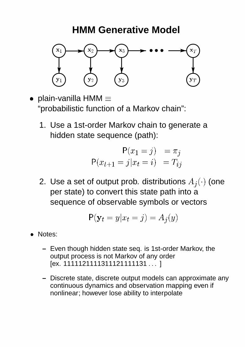
� � plain-vanilla HMM �

“probabilistic function of a Markov chain”:

1. Use a 1st-order Markov chain to generate ahidden state sequence (path): �������� ��� � ���

�������� � � � �!� � � "#� � $&% �2. Use a set of output prob. distributions ' �(�*)+� (one

per state) to convert this state path into asequence of observable symbols or vectors ���, � � -.�/� � � ���0� ' �1��-2�

3 Notes:

– Even though hidden state seq. is 1st-order Markov, theoutput process is not Markov of any order[ex. 1111121111311121111131 4#454 ]

– Discrete state, discrete output models can approximate anycontinuous dynamics and observation mapping even ifnonlinear; however lose ability to interpolate

LDS Generative Model

PSfrag replacements

6�7

8�7

6�9

8�9

6�:

8 :

6�;

8 ;< Gauss-Markov continuous state process:

=?>�@BADC E = >&F G >observed through the “lens” of anoisy linear embedding:

H > C I = >JF KL>< Noises G M and KNM are temporally white and

uncorrelated with everything else< Think of this as “matrix flow in a pancake”

(Also called state-space models, Kalman filter models.)

EM applied to HMMs and LDSs

X 3

Y3

XO

1

Y1

XO

2

Y2

XO

T

YT

Given a sequence of P observations Q�RNSUTWVXVWV�TYRJZ�[E-step . Compute the posterior probabilities:\ HMM: Forward-backward algorithm: ] ^_Q�`a[cbdQ�eD[gf\ LDS: Kalman smoothing recursions: ] ^_Qihj[cb+Q�eD[gfM-step . Re-estimate parameters:\ HMM: Count expected frequencies.\ LDS: Weighted linear regression.

Notes:1. forward-backward and Kalman smoothing recursions

are special cases of belief propagation.

2. online (causal) inference ] ^�`�kUb+Q�R S TiVXVWV�TYRlk5[gf is doneby the forward algorithm or the Kalman filter.

3. what sets the (arbitrary) scale of the hidden state?Scale of m (usually fixed at n ).

Trees/Chains

o Tree-structured p each node has exactly one parent.

o Discrete nodes or linear-Gaussian.

o Hybrid systems are possible: mixed discrete &continuous nodes. But, to remain tractable, discretenodes must have discrete parents.

o Exact & efficient inference is done by beliefpropagation (generalised Kalman Smoothing).

o Can capture multiscale structure (e.g. images)

Polytrees/La yered Networks

q more complex models for which junction-treealgorithm would be needed to do exact inference

q discrete/linear-Gaussian nodes are possible

q case of binary units is widely studied:Sigmoid Belief Networks

q but usually intractable

Intractability

For many probabilistic models of interest, exact inferenceis not computationally feasible.This occurs for two (main) reasons:

r distributions may have complicated forms(non-linearities in generative model)r “explaining away” causes coupling from observationsobserving the value of a child induces dependenciesamongst its parents (high order interactions)

Y

X3 X4X1 X5X2

1 2 311

Y = X1 + 2 X2 + X3 + X4 + 3 X5

We can still work with such models by using approximateinference techniques to estimate the latent variables.

Appr oximate Inference

s Sampling :approximate true distribution over hidden variableswith a few well chosen samples at certain values

s Linearization :approximate the transformation on the hiddenvariables by one which keeps the form of thedistribution closed (e.g. Gaussians and linear)

s Recognition Models :approximate the true distribution with anapproximation that can be computed easily/quicklyby an explicit bottom-up inference model/network

s Variational Methods :approximate the true distribution with an approximateform that is tractable; maximise a lower bound on thelikelihood with respect to free parameters in this form

Sampling

Gibbs Sampling

To sample from a joint distribution t uwv�x�yzv|{�yW}X}W}�yzv�~ � :Start from some initial state ����� u�v�� x y�v��{ yi}X}W}�yzv��~ � :Then iterate the following procedure:

� Pick �������� from ����� �*� � ���� � �� � � �� �#�5�5�1� � ����� Pick �������� from ����� � � �������� � � �� � � �� �#�5�5�1� � ����� ...

� Pick �������� from ����� � � �������� � �������� � �������� �#�5�#��� ��������2� � �This procedure goes from ��� � � �W¡ x , creating a Markovchain which converges to t u¢� �Gibbs sampling can be used to estimate the expectationsunder the posterior distribution needed for E-step of EM.

It is just one of many Markov chain Monte Carlo (MCMC)methods. Easy to use if you can easily update subsets oflatent variables at a time.

Key questions: how many iterations per sample?how many samples?

Partic le Filter s

Assume you have £ weighted samples ¤�¥+¦�§©¨ ª¬«®­ §°¯¥+¦�§²±5³#³5³1± «®­µ´ ¯¥+¦i§·¶ from¸�¹dº ¥+¦�§¼»µ½�¥+¦i§¿¾ , with normalised weights À ­µÁ ¯¥+¦i§1. generate a new sample set ¤�Â¥+¦i§ by sampling with replacement

from ¤ ¥+¦i§ with probabilities proportional to Àí!Á ¯¥+¦i§2. for each element of ¤  predict , using the stochastic dynamics,

by sampling «®­!Á ¯¥ from¸�¹dº ¥ » º ¥+¦i§ ¨ «®­µÁ ¯ Â¥+¦i§ ¾

3. Using the measurement model, weight each new sample by

ÀíµÁ ¯¥ ¨ ¸�¹ÅÄ ¥Æ» º ¥ ¨ «®­µÁ ¯¥ ¾(the likelihoods) and normalise so that Ç Á Àí!Á ¯¥ ¨ È .

Samples need to be weighted by the ratio of the distribution we drawthem from to the true posterior (this is importance sampling).

An easy way to do that is draw from prior and weight by likelihood.

(Also known as CONDENSATION algorithm.)

Linearization

Extended Kalman Filtering and Smoothing

UÉ1 U

É2 U

É3 U

É4

XÊ1 X

Ê2 X

Ê3 X

Ê4

Y1 Y2 Y3 Y4

Ë?Ì·Í0Î�Ï Ð�Ñ�Ë ÌÓÒÓÔ�ÌÖÕ&× Ø ÌÙ Ì Ï Ú|Ñ¢Ë Ì¬ÒÓÔ.ÌÖÕ&× Û?Ì

Linearise about the current estimate, i.e. given ÜË Ì¬Ò®Ô.Ì :Ë Ì�Í0ÎÞÝ Ð Ñ ÜË Ì¬ÒßÔ�ÌàÕ&× á Ð

á Ë Ìâââââ¿ãäæå Ñ�Ë Ìaç ÜË ÌÖÕ|× Ø Ì

Ù Ì Ý Ú|Ñ ÜË Ì¬ÒßÔ.ÌàÕ&× á Úá Ë Ì

âââââwãä å Ñ¢Ë Ìaç ÜË ÌÖÕ&× Û?Ì

Run the Kalman smoother (belief propagation forlinear-Gaussian systems) on the linearised system. Thisapproximates non-Gaussian posterior by a Gaussian.

Recognition Models

è a function approximator is trained in a supervisedway to recover the hidden causes (latent variables)from the observations

è this may take the form of explicit recognition network(e.g. Helmholtz machine) which mirrors thegenerative network (tractability at the cost ofrestricted approximating distribution)

è inference is done in a single bottom-up pass(no iteration required)

Variational Inference

Goal: maximise é�êìë í¿î ïñðóò .Any distribution ô í�õ ò over the hidden variables defines alower bound on é�êìë íwî ïöðæò :

é�ê÷ë íwî ïñðóò�ø ù ô í�õ ò1éÅê ë í�õ úYî ïöðóòô í�õ ò û

ü íýô ú¬ðóò

Constrain ô í�õ ò to be of a particular tractable form (e.g.factorised) and maximise

üsubject to this constraint

þ E-step: Maximiseü

w.r.t. ô with ð fixed, subject tothe constraint on ô , equivalently minimise:

éÅêÿë íwî ïöðóò�� ü íýô ú¬ðóò û ù ô í�õ ò1é�ê ô íwõ òë í�õ ï/î ò

û KL íýô � ë òThe inference step therefore tries to find ô closest tothe exact posterior distribution.

þ M-step: Maximiseü

w.r.t. ð with ô fixed

(related to mean-field approximations)

Beyond Maxim um Likelihood:Finding Model Structure and Avoiding Overfitting

0 5 10−20

0

20

40

M = 1

0 5 10−20

0

20

40

M = 2

0 5 10−20

0

20

40

M = 3

0 5 10−20

0

20

40

M = 4

0 5 10−20

0

20

40

M = 5

0 5 10−20

0

20

40

M = 6

Model Selection Questions

How many clusters in this data set?

What is the intrinsic dimensionality of the data?

What is the order of my autoregressive process?

How many sources in my ICA model?

How many states in my HMM?

Is this input relevant to predicting that output?

Is this relationship linear or nonlinear?

Bayesian Learning and Ockham’ s Razor

data � , models � ��������� , parameter sets ���������� (let’s ignore hidden variables � for the moment; they will just

introduce another level of averaging/integration)

Total Evidence:� ��� � � � � ��� � � � � � � �Model Selection:� � ����� ��� � ��� � ��� � � ���� ��� �

� ��� � ��� � � � ��� �"!#�$ �%�&� �'!(��� ���) � ��� � � �

is the probability that randomly selectedparameter values from model class

�would

generate data set�

.) Model classes that are too simple will be veryunlikely to generate that particular data set.) Model classes that are too complex can generatemany possible data sets, so again, they are unlikelyto generate that particular data set at random.

Ockham’ s Razor

too simple

too complex

"just right"

Data Sets

P(D

ata)

Y

(adapted from D.J.C. MacKay)

Overfitting

0 5 10−20

0

20

40

M = 1

0 5 10−20

0

20

40

M = 2

0 5 10−20

0

20

40

M = 3

0 5 10−20

0

20

40

M = 4

0 5 10−20

0

20

40

M = 5

0 5 10−20

0

20

40

M = 6

0 1 2 3 4 5 60

0.2

0.4

0.6

0.8

1

M

P(M

)

Practical Bayesian Appr oaches

* Laplace approximations* Large sample approximations (e.g. BIC)* Markov chain Monte Carlo methods* Variational approximations

Laplace Appr oximation

data set + , models , -/..�.102, 3 , parameter sets 4�-�...�0�43Model Selection:5 6 7�8�9 :<; 5 6 7�:&5 6�9 8 7�:For large amounts of data (relative to number ofparameters, = ) the parameter posterior is approximatelyGaussian around the MAP estimate >? 7 :@BA 4CEDF+G0�, CIHKJ AMLON HQPSRT DVUWDYXT[Z2\^]`_badcL A 4C a e4CIHgfhU A 4C a e4CiHj

5 6�9 8 7 :lk 5 6 ? 7Qm 9 8 7 :5 6 ? 7 8n9 m 7 :Evaluating the above expression for oip 5 6�9 8 7 :

at >? 7 :q"r @BA + DF, C HKJ q"r @BA e4 C DF, C Hts q"r @BA +uD e4 C 02, C Hts v L q"r LON a cL q"r DVUWDwhere w is the negative Hessian of the log posterior.

This can be used for model selection.(Note: w is size = x = .)

BIC

The Bayesian Information Criterion (BIC) can be obtainedfrom the Laplace approximationy"z|{B}i~ �F� �I�K� y"z|{B}��� ���F� �I�t� y"z|{B}i~u���� ���2� �I�t� � ��y"z �O�u� ���y"z��V�W�by taking the large sample limit:���W� ��� � ����� ����� ��� ���  �¡ �%�G¢ £ ¤¥���W¦where

¦is the number of data points.

Properties:§ Quick and easy to compute§ It does not depend on the prior§ We can use the ML estimate of 

instead of the MAPestimate§ It assumes that in the large sample limit, all theparameters are well-determined (i.e. the model isidentifiable; otherwise, £ should be the number ofwell-determined parameters)§ It is equivalent to the MDL criterion

MCMC

Assume a model with parameters ¨ , hidden variables ©and observable variables ªGoal: to obtain samples from the (intractable) posteriordistribution over the parameters, « ¬'¨®­�ª ¯Approach: to sample from a Markov chain whoseequilibrium distribution is « ¬'¨®­nª ¯ .One such simple Markov chain can be obtained by Gibbssampling, which alternates between:° Step A: Sample from parameters given hidden

variables and observables: ¨ ± « ¬'¨®­n© ²³ª ¯° Step B: Sample from hidden variables givenparameters and observables: © ± « ¬E© ­´¨K²³ª ¯

Note the similarity to the EM algorithm!

Variational Bayesian Learning

Lower bound the evidence:µ ¶ ·i¸º¹ »�¼ ½¾ ·i¸ ¹ »�¼B¿�À�½ÂÁÃÀÄ Å »'À�½1·i¸ ¹ »�¼B¿�ÀƽŠ»ÇÀƽ ÁÃÀ¾ Å »'À�½ÉÈ ·�¸�¹ »�¼ Ê´À�½ Ë ·�¸ ¹ »'À�½Å »'À�½�Ì Á1ÀÄ Å »'À�½ È È Å »EÍ ½1·i¸ ¹ »�Í ¿³¼ Ê´À�½Å »EÍ ½ Á�Í Ì Ë ·i¸ ¹ »ÇÀƽŠ»'À�½ Ì ÁÃÀ¶ Î » Å »'À�½�¿ Å »EÍ ½h½

Assumes the factorisation:¹ »ÇÀÏ¿OÍ Ê�¼ ½<Ð Å »'À�½ Å »EÍ ½(also known as “ensemble learning”)

Variational Bayesian Learning

EM-like optimisation:

“E-step” : Maximise Ñ w.r.t. Ò ÓEÔ Õ with Ò Ó'Ö�Õ fixed

“M-step” : Maximise Ñ w.r.t. Ò ÓÇÖÆÕ with Ò ÓEÔ Õ fixed

Finds an approximation to the posterior over parametersÒ Ó'Ö�Õl× Ø Ó'Ö®Ù�Ú Õ and hidden variables Ò ÓEÔ Õ�× Ø ÓEÔ Ù�Ú ÕÛ Maximises a lower bound on the log evidenceÛ Convergence can be assessed by monitoring ÑÛ Global approximationÛ Ñ transparently incorporates model complexitypenalty (i.e. coding cost for all the parameters of themodel) so it can be compared across modelsÛ Optimal form of Ò Ó'Ö�Õ falls out of free-form variationaloptimisation (i.e. not assumed to be Gaussian)Û Often simple modification of the EM algorithm

Summar y

Ü Why probabilistic models?Ü Factor analysis and beyondÜ Inference and the EM algorithmÜ Generative Model for Generative ModelsÜ A few models in detailÜ Approximate inferenceÜ Practical Bayesian approaches

Appendix

Desiderata (or Axioms) for

Computing Plausibilities

Paraphrased from E.T. Jaynes, using the notation Ý�Þ'ß àâá ãis the plausibility of statement ß given that you know thatstatement á is true.ä Degrees of plausibility are represented by real

numbersä Qualitative correspondence with common sense, e.g.

– If Ý�ÞÇß àæå çgãéè Ý�ÞÇß àæå ã but Ý�Þ2á à"ß ê å çëãlì Ý�Þ2á à´ß êíå ãthen Ý�ÞÇß ê á àâå ç ãéî Ý�Þ'ß ê á àæå ãä Consistency:

– If a conclusion can be reasoned in more than oneway, then every possible way must lead to thesame result.

– All available evidence should be taken intoaccount when inferring a plausibility.

– Equivalent states of knowledge should berepresented with equivalent plausibilitystatements.

Accepting these desiderata leads to Bayes Rule beingthe only way to manipulate plausibilities.

Learning with Complete Data

Y1

θ1

θ3θ2

θ4

Yï

2 Yï

3

Y4

Assume a data set of i.i.d. observationsð ñ òôó õEö&÷�ø#ùúù#ù�ø�ó õ�û�÷&üand a parameter vector ý .

Goal is to maximise likelihood: þ ÿ ð � ý�� ñ û��� ö þ ÿ ó õ � ÷ � ý��Equivalently, maximise log likelihood:� ÿ'ý�� ñ û��� ö � þ ÿ ó õ � ÷ � ý��Using the graphical model factorisation:þ ÿ ó õ � ÷ � ý�� ñ � þ ÿ ó õ � ÷� ��ó õ � ÷

pa(

�)ø ý � �

So:� ÿ'ý�� ñ û��� ö � � þ ÿ ó õ � ÷� �nó õ � ÷

pa(

�)ø ý � �

In other words, the parameter estimation problem breaksinto many independent, local problems (uncoupled).

Building a Junction Tree

� Start with the recursive factorization from the DAG:����� ��� � ����� ���pa( ��� ) �

� Convert these local conditional probabilities intopotential functions over both

� �and all its parents.� This is called moralising the DAG since the parents

get connected. Now the product of the potentialfunctions gives the correct joint� When evidence is absorbed, potential functions mustagree on the prob. of shared variables: consistency.� This can be achieved by passing messages betweenpotential functions to do local marginalising andrescaling.� Problem: a variable may appear in twonon-neighbouring cliques. To avoid this we need totriangulate the original graph to give the potentialfunctions the running intersection property.Now local consistency will imply global consistency.

Bayesian Networks: Belief Propagation

p1 p2p3

c1c2 c3

n

e (n)+�

e (n)-

Each node � divides the evidence, � , in the graph intotwo disjoint sets: �! #"��%$ and �'&("��%$Assume a node � with parents )�*,+.-0/1/0/�-2*43�5 and)768+9-1/0/1/�-:6�;95<>= ?A@CBED F GH IKJ2LKMONPNPNQM JSRUT9<>= ?A@ VXWSY[Z\Z\Z]Y^V8_`D _

acb W <>=cV a @CB\de=fV a D�Dhgi jklmb W <>=Un l Y2Bpo�=Un l Dq@P?]DF <>=?4@CB\dr=?]D�Dm<>=UBpo�=?]Dq@P?]D

ICA Nonlinearity

Generative model:s t uwv�x yz t { s | }where x and } are zero-mean Gaussian noiseswith covariances ~ and �respectively.

−5 −4 −3 −2 −1 0 1 2 3 4 5−15

−10

−5

0

5

10

15

w

g(w

)

The density of � can be written in terms of uwvq��y ,��� v � y�t � v��r����y,���7���E� �'���ue��v�uA���9v � y�y9�

For example, if � � v � y�t ����¡ E¢m£ � �'� we find that setting:

uwv�¤ y�t ¥¦ §8¨ª©«¦ §­¬ ® ¯9�°| ±.²´³�v�¤ µe¶ ·8y¡¸�¹º¹generates vectors s in which each component isdistributed exactly according to ��µ»v ¬ ¼¾½«¿ÁÀ v � y�y .So, ICA can be seen either as a linear generative modelwith non-Gaussian priors for the hidden variables, or as anonlinear generative model with Gaussian priors for thehidden variables.

HMM Example Character sequences (discrete outputs)

−*

9

A B C D EF GH I J

K L M N O

P Q R STU V WX Y

−*

9

AB C D E

F G H IJ

K L M N OP Q R S T

U V W X Y

−

*

9

A BCD E

F G H I J

K L MNO

P Q R STUVWX Y

−

*

9

AB C D EF G H I J

K L M N O

P Q R STU V W X Y

 Geyser data (continuous outputs)

0.5 1 1.5 2 2.5 3 3.5 4 4.5 5 5.540

50

60

70

80

90

100

110

y1

y2

State output functions

LDS Example

à Population model:state Ä population histogramfirst row of A Ä birthratessubdiagonal of A Ä 1-deathratesQ Ä immigration/emmigrationC Ä noisy indicators

Noi

sy M

easu

rem

ents

50 100 150 200 250 300 350 400 450 0

50

100

150

200

250

Infe

rred

Pop

ulat

ion

50 100 150 200 250 300 350 400 450 0

50

100

150

200

250

Time

Tru

e P

opul

atio

n

Viterbi Decoding

Å The numbers ÆÈÇrÉ�ÊªË in forward-backward gave theposterior probability distribution over all states at anytime.

Å By choosing the state Æ�ÌÈÉ�ÊEË with the largestprobability at each time, we can make a “best” statepath. This is the path with themaximum expected number of correct states.

Å But it is not the single path with the highest likelihoodof generating the data.In fact it may be a path of probability zero!

Å To find the single best path, we do Viterbi decodingwhich is just Bellman’s dynamic programmingalgorithm applied to this problem.

Å The recursions look the same, except withÍ Î9Ï instead of Ð .

Å There is also a modified Baum-Welch training basedon the Viterbi decode.

HMM PseudocodeÑ Forward-backward including scaling tricksÒhÓ2ÔÖÕh׫ØÚÙXÓÛÔÝܾÞß×à'ÔUáâ×ãØÚä0å¡æÈÒEÔUáâ× çèÔUáâ×ãØ à'Ôéá�× à'ÔUáâ׫ØÚà'Ôéá�×hêÛçèÔéá�×à'ÔÖÕh×«Ø Ôßëíì`æ'à'ÔÖÕ!îïáâ×é×�å2æÈÒÁÔÖÕh× çèÔÖÕé×8Ø à'ÔßÕé× à'ÔÖÕh×8ØÚà'ÔßÕé×éê2çèÔÖÕh× ðñÕ8Øóòõô÷ö[øù ÔÝöp×«Ø áù ÔÖÕh׫Øïë#æúÔ ù ÔÖÕüûýáâ×�åÛæ'ÒÁÔÖÕ�ûÚáâ×é×éê2çèÔÖÕ.ûþáâ× ðñÕ8Ø ÔÝöAîïáâ×ÿô:á�ø� Ø��� Ø � û ë�å2æ Ô à'ÔßÕé×9æúÔ ù ÔßÕüûýá�×�åÛæÈÒEÔÖÕ�ûÚáâ×é× ì ×hêÛçèÔßÕ.ûþá�× ðñÕ8Ø á­ôèÔÝö îÚáâ×ø��Ø Ô à7å´æ ù ×����� ÔßÜ�� �×8Ø ����� ÔÝçèÔÖÕé×h×

Ñ Baum-Welch parameter updates

� Ó Ø�� �ë�� Ó Ø�� �ä Ø�� �ÙýØ��for each sequence, run forward backward to get � and

�, then

�ëÚØ �ë û � �ä Ø �ä û��ãÔUáâ× � Ø � û Þ �!ÔßÕé×�Ù Ó ÔÝÜ0×«Ø Þ�� ������� � Ó ÔÖÕé× or �ÙóØ �Ù#û Þ Ü Þ �ãÔÖÕh×�ë � ÓXØ �ë � Ó�ê

��ë � � �ä Ø �ä�ê �ä �Ù'ÓXØ �ÙXÓ�ê � Ó

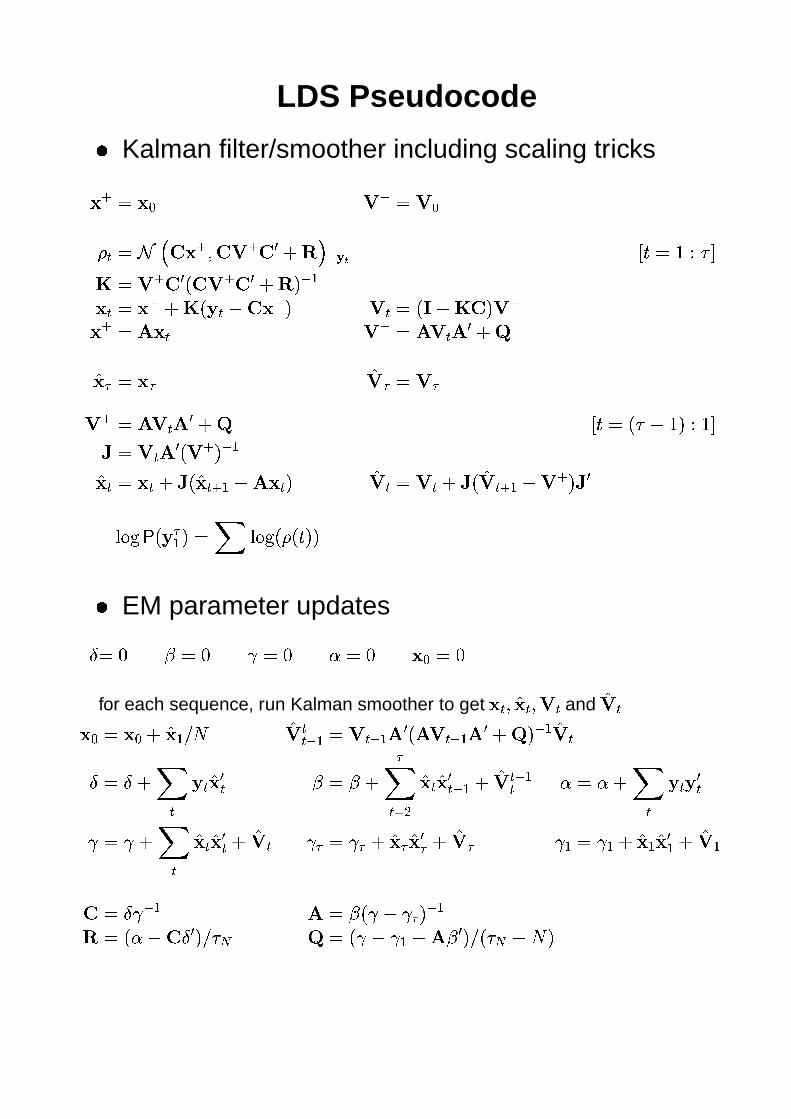
LDS Pseudocode� Kalman filter/smoother including scaling tricks

�! #"$�&% '( )"*')%+�, ".- /102� 43 05' 056�798):<;>=�? @BAC" DFEHGJIK "L' 0 6NM 05' 0 6 798)OQPSR� , "$� 7 K M�TU,WV 02� O ' , " MNXYV K 0ZO[' �! #"*\]� , '( )"�\' , \ 6 7_^`�Uab"$��a `'ca"*'ca' "*\' , \ 6 7_^ @BAC" M G V DdOeEWD�If "L' , \ 6gM ' OQPSR`� , "$� , 7 f M `� , R V \h� , O `' , "*' , 7 f M `' , R V ' O f 6i�j�kl M�T a R Om" i�j�k MN+�M AQOnO

� EM parameter updateso "*p qr"�p s#"�p tr"�p ��%Y"�p

for each sequence, run Kalman smoother to get � , 3 `� , 3 ' , and`' ,

� % "L� % 7 `� Rnu1v `' ,, PSR "w' , PSR \ 6gM \' , PSR \ 6 7$^]OQPSR `' ,o " o 7

,T , `� 6, qr"Lqx7

a,�y{z

`� , `� 6, PSR 7 `' , PSR, t|"�t)7,T , T&6,

s#"ws}7,

`� , `� 6, 7 `' , s~a�"ws~a�7 `�Ua `� 6a 7 `'ca s R "*s R 7 `� R `� 6 R 7 `' R

0 " o s&PSR \ "Lq M s V s~a�OQPSR8 " M t V 0 o 6�O u G�� ^ " M s V s R V \]q&6�O u M G�� V v O

Selected References

Graphical Models and the EM algorithm:

� Learning in Graphical Models (1998) Edited by M.I. Jordan. Dordrecht:Kluwer Academic Press. Also available from MIT Press (paperback).

� Motiv ation for Bayes Rule : ”Probability Theory - the Logic of Science,”E.T.Jaynes, http://www.math.albany.edu:8008/JaynesBook.html

� EM:

Baum, L., Petrie, T., Soules, G., and Weiss, N. (1970). A maximizationtechnique occurring in the statistical analysis of probabilistic functions ofMarkov chains. The Annals of Mathematical Statistics, 41:164–171;

Dempster, A., Laird, N., and Rubin, D. (1977).Maximum likelihood from incomplete data via the EM algorithm.J. Royal Statistical Society Series B, 39:1–38;

Neal, R. M. and Hinton, G. E. (1998).A new view of the EM algorithm that justifies incremental, sparse, and othervariants. In Learning in Graphical Models.

� Factor Anal ysis and PCA:

Mardia, K.V., Kent, J.T., and Bibby J.M. (1979)Multivariate Analysis Academic Press, London

Roweis, S. T. (1998). EM algorthms for PCA and SPCA. NIPS98

Ghahramani, Z. and Hinton, G. E. (1996). The EM algorithm for mixtures offactor analyzers. Technical Report CRG-TR-96-1[http://www.gatsby.ucl.ac.uk/ � zoubin/papers/tr-96-1.ps.gz]Department of Computer Science, University of Toronto.

Tipping, M. and Bishop, C. (1999). Mixtures of probabilistic principalcomponent analyzers. Neural Computation, 11(2):435–474.

� Belief propagation:

Kim, J.H. and Pearl, J. (1983) A computational model for causal anddiagnostic reasoning in inference systems.In Proc of the Eigth International Joint Conference on AI: 190-193;

Pearl, J. (1988). Probabilistic Reasoning in Intelligent Systems: Networks ofPlausible Inference. Morgan Kaufmann, San Mateo, CA.

� Junction tree: Lauritzen, S. L. and Spiegelhalter, D. J. (1988).Local computations with probabilities on graphical structures and theirapplication to expert systems. J. Royal Statistical Society B, pages 157–224.

Other graphical models:

� Roweis, S.T and Ghahramani, Z. (1999) A unifying review of linear Gaussianmodels. Neural Computation 11(2): 305–345.

� ICA:

Comon, P. (1994). Independent component analysis: A new concept.Signal Processing, 36:287–314;

Baram, Y. and Roth, Z. (1994) Density shaping by neural networks withapplication to classification, estimation and forecasting.Technical Report TR-CIS-94-20, Center for Intelligent Systems, Technion,Israel Institute for Technology, Haifa, Israel.

Bell, A. J. and Sejnowski, T. J. (1995). An information-maximizationapproach to blind separation and blind deconvolution.Neural Computation, 7(6):1129–1159.

� Trees:

Chou, K.C., Willsky, A.S., Benveniste, A. (1994)Multiscale recursive estimation, data fusion, and regularization.IEEE Trans. Automat. Control 39:464-478;

Bouman, C. and Shapiro, M. (1994).A multiscale random field model for Bayesian segmenation.IEEE Transactions on Image Processing 3(2):162–177.

� Sigmoid Belief Networks:

Neal, R. M. (1992). Connectionist learning of belief networks.Artificial Intelligence, 56:71–113.

Saul, L.K. and Jordan, M.I. (1999) Attractor dynamics in feedforward neuralnetworks. To appear in Neural Computation.

Appr oximate Inference & Learning� MCMC: Neal, R. M. (1993). Probabilistic inference using Markov chainmonte carlo methods. Technical Report CRG-TR-93-1,Department of Computer Science, University of Toronto.

� Partic le Filter s:

Gordon, N.J. , Salmond, D.J. and Smith, A.F.M. (1993)A novel approach to nonlinear/non-Gaussian Bayesian state estimationIEE Proceedings on Radar, Sonar and Navigation 140(2):107-113;

Kitagawa, G. (1996) Monte Carlo filter and smoother for non-Gaussiannonlinear state space models,Journal of Computational and Graphical Statistics 5(1):1–25.

Isard, M. and Blake, A. (1998) CONDENSATION – conditional densitypropagation for visual tracking Int. J. Computer Vision 29 1:5–28.

� Extended Kalman Filtering: Goodwin, G. and Sin, K. (1984).Adaptive filtering prediction and control. Prentice-Hall.

� Recognition Models:

Hinton, G. E., Dayan, P., Frey, B. J., and Neal, R. M. (1995). The wake-sleepalgorithm for unsupervised neural networks. Science, 268:1158–1161.

Dayan, P., Hinton, G. E., Neal, R., and Zemel, R. S. (1995)The Helmholtz Machine . Neural Computation, 7, 1022-1037.

� Ockham’ s Razor and Laplace Appr oximation:

Jefferys, W.H., Berger, J.O. (1992)Ockham’s Razor and Bayesian Analysis. American Scientist 80:64-72;

MacKay, D.J.C. (1995) Probable Networks and Plausible Predictions -A Review of Practical Bayesian Methods for Supervised Neural Networks.Network: Computation in Neural Systems. 6 469-505

� BIC: Schwarz, G. (1978). Estimating the dimension of a model.Annals of Statistics 6:461-464.

� MDL: Wallace, C.S. and Freeman, P.R. (1987) Estimation and inference bycompact coding. J. of the Royal Stat. Society series B 49(3): 240-265;J. Rissanen (1987)

� Bayesian Gibbs sampling software:The BUGS Project – http://www.iph.cam.ac.uk/bugs/

� Variational Bayesian Learning:

Hinton, G. E. and van Camp, D. (1993) Keeping Neural Networks Simple byMinimizing the Description Length of the Weights.In Sixth ACM Conference on Computational Learning Theory, Santa Cruz.

Waterhouse, S., MacKay, D., and Robinson, T. (1995)Bayesian methods for Mixtures of Experts. NIPS95.(See also several unpublished papers by MacKay).

Bishop, C.M. (1999) Variational PCA. In Proc. Ninth Int. Conf. on ArtificialNeural Networks ICANN99 1:509 - 514.

Attias, H. (1999). Inferring parameters and structure of latent variablemodels by variational Bayes. In Proc. 15th Conf. on Uncertainty in ArtificialIntelligence;

Ghahramani, Z. and Beal, M.J. (1999)Variational Bayesian Inference for Mixture of Factor Analysers. NIPS99;

http://www.gatsby.ucl.ac.uk/