“probabilistic logic programs and their applications”
TRANSCRIPT

Probabilistic (Logic) Programming and its
ApplicationsLuc De Raedt
with many slides from Angelika Kimmmig

A key question in AI:Dealing with uncertainty
Reasoning with relational data
Learning
Statistical relational learning& Probabilistic Programming
?• logic• databases• programming• ...
• probability theory• graphical models• ...
• parameters• structure
2

The need for relations

Dynamics: Evolving Networks
• Travian: A massively multiplayer real-time strategy game
• Commercial game run by TravianGames GmbH
• ~3.000.000 players spread over different “worlds”
• ~25.000 players in one world[Thon et al. ECML 08]
4

World Dynamics
border
border
border
border
Alliance 2
Alliance 3
Alliance 4
Alliance 6
P 2
1081
8951090
1090
1093
1084
1090
915
1081
1040
770
1077
955
1073
8041054
830
9421087
786
621
P 3
744
748559
P 5
861
P 6
950
644
985
932
837871
777
P 7
946
878
864 913
P 9
Fragment of world with
~10 alliances~200 players~600 cities
alliances color-coded
Can we build a modelof this world ?
Can we use it for playingbetter ?
[Thon, Landwehr, De Raedt, ECML08]
5

World Dynamics
border
border
border
border
Alliance 2
Alliance 4
Alliance 6
P 2
9041090
917
770
959
1073
820
762
9461087
794
632
P 3
761
961
1061
607
988
771
924
583
P 5
951
935
948
938
867
P 6
950
644
985
888
844875
783
P 7
946
878
864 913
Fragment of world with
~10 alliances~200 players~600 cities
alliances color-coded
Can we build a modelof this world ?
Can we use it for playingbetter ?
[Thon, Landwehr, De Raedt, ECML08]
6

World Dynamics
border
border
border
border
Alliance 2
Alliance 4
Alliance 6
P 2
9181090
931
779
977
835
781
9581087
808
701
P 3
838
947
1026
1081
833
1002987
827
994
663
P 5
1032
1026
1024
1049
905
926
P 6
986
712
985
920
877
807
P 7
895
959
P 10
824
Fragment of world with
~10 alliances~200 players~600 cities
alliances color-coded
Can we build a modelof this world ?
Can we use it for playingbetter ?
[Thon, Landwehr, De Raedt, ECML08]
7

Analyzing Video Data
• Track people or objects over time? Even if temporarily hidden?
• Recognize activities?
• Infer object properties?
Fig. 4. Tracking results from experiment 2. In frame 5, two groups arepresent. In frame 15, the tracker has correctly split group 1 into 1-0 and 1-1(see Fig. 3). Between frames 15 and 29, group 1-0 has split up into groups1-0-0 and 1-0-1, and split up again. New groups, labeled 2 and 3, enter thefield of view in frames 21 and 42 respectively.
Six frames of the current best hypothesis from experiment2 are shown in Fig. 4, the corresponding hypothesis tree isshown in Fig. 3. The sequence exemplifies movement andformation of several groups.
A. Clustering Error
Given the ground truth information on a per-beam basis wecan compute the clustering error of the tracker. This is doneby counting how often a track’s set of points P contains toomany or wrong points (undersegmentation) and how often Pis missing points (oversegmentation) compared to the groundtruth. Two examples for oversegmentation errors can be seenin Fig. 4, where group 0 and group 1-0 are temporarilyoversegmented. However, from the history of group splitsand merges stored in the group labels, the correct group
0
0.1
0.2
0.3
0.4
0.5
0.6
0.5 1 1.5 2 2.5 3 3.5
Err
or
rate
s p
er
tra
ck a
nd f
ram
e
Clustering distance threshold dP (m)
w/o tracking
Overs. + Unders.Oversegm.
Undersegm.
0
0.2
0.4
0.6
0.8
1
0 4 8 12 16 20
Avg
. cycle
tim
e (
se
c)
Number of people in ground truth
Group trackerPeople tracker
Fig. 5. Left: clustering error of the group tracker compared to a memory-less single linkage clustering (without tracking). The smallest error isachieved for a cluster distance of 1.3 m which is very close to the border ofpersonal and social space according to the proxemics theory, marked at 1.2m by the vertical line. Right: average cycle time for the group tracker versusa tracker for individual people plotted against the ground truth number ofpeople.
relations can be determined in such cases.For experiment 1, the resulting percentages of incorrectly
clustered tracks for the cases undersegmentation, overseg-mentation and the sum of both are shown in Fig. 5 (left),plotted against the clustering distance dP . The figure alsoshows the error of a single-linkage clustering of the rangedata as described in section II. This implements a memory-less group clustering approach against which we comparethe clustering performance of our group tracker.
The minimum clustering error of 3.1% is achieved by thetracker at dP = 1.3 m. The minimum error for the memory-less clustering is 7.0%, more than twice as high. In themore complex experiment 2, the minimum clustering errorof the tracker rises to 9.6% while the error of the memory-less clustering reaches 20.2%. The result shows that thegroup tracking problem is a recursive clustering problem thatrequires integration of information over time. This occurswhen two groups approach each other and pass from oppositedirections. The memory-less approach would merge themimmediately while the tracking approach, accounting for thevelocity information, correctly keeps the groups apart.
In the light of the proxemics theory the result of a minimalclustering error at 1.3 m is noteworthy. The theory predictsthat when people interact with friends, they maintain a rangeof distances between 45 to 120 cm called personal space.When engaged in interaction with strangers, this distance islarger. As our data contains students who tend to know eachother well, the result appears consistent with Hall’s findings.
B. Tracking Efficiency
When tracking groups of people rather than individuals,the assignment problems in the data association stage areof course smaller. On the other hand, the introduction ofan additional tree level on which different models hypoth-esize over different group formation processes comes withadditional computational costs. We therefore compare oursystem with a person-only tracker which is implemented byinhibiting all split and merge operations and reducing thecluster distance dP to the very value that yields the lowesterror for clustering single people given the ground truth. For
8
[Skarlatidis et al, TPLP 14; Nitti et al, IROS 13, ICRA 14]

Learning relational affordancesLearn probabilistic model
From two object interactions Generalize to N
Shelf
push
Shelftap
Shelf
grasp
Moldovan et al. ICRA 12, 13, 14, PhD 15

Learning relational affordancesLearn probabilistic model
From two object interactions Generalize to N
Shelf
push
Shelftap
Shelf
grasp
Moldovan et al. ICRA 12, 13, 14, PhD 15

Example: Information Extraction
10 NELL: http://rtw.ml.cmu.edu/rtw/

Example: Information Extraction
10 NELL: http://rtw.ml.cmu.edu/rtw/
instances for many different relations

Example: Information Extraction
10 NELL: http://rtw.ml.cmu.edu/rtw/
instances for many different relations
degree of certainty
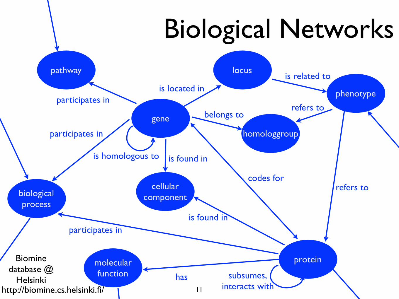
codes for
gene
protein
pathway
cellularcomponent
homologgroup
phenotype
biologicalprocess
locus
molecularfunction has
is homologous to
participates in
participates inis located in
is related to
refers tobelongs to
is found in
subsumes,interacts with
is found in
participates in
refers to
Biomine database @
Helsinki
Biological Networks
11http://biomine.cs.helsinki.fi/

• Structured environments
• objects, and
• relationships amongst them
• and possibly
• using background knowledge
• cope with uncertainty
• learn from data
This requires dealing with
12
Statis
tical
Relatio
nal L
earn
ing
Prob
abilis
tic Pr
ogra
mming

Common themeDealing with uncertainty
Reasoning with relational data
Learning
Statistical relational learning& Probabilistic Programming, ...
13

Some formalisms
14
Some SRL formalisms
LPAD: Bruynooghe
Vennekens,VerbaetenMarkov Logic: Domingos,
Richardson
CLP(BN): Cussens,Page,
Qazi,Santos Costa
Present
PRMs: Friedman,Getoor,Koller,
Pfeffer,Segal,Taskar
´03
SLPs: Cussens,Muggleton
´90 ´95 96
First KBMC approaches:
Breese,
Bacchus,
Charniak,
Glesner,
Goldman,
Koller,
Poole, Wellmann
´00
BLPs: Kersting, De Raedt
RMMs: Anderson,Domingos,
Weld
LOHMMs: De Raedt, Kersting,
Raiko
Future
Prob. CLP: Eisele, Riezler
´02
PRISM: Kameya, Sato
´94
PLP: Haddawy, Ngo
´97´93
Prob. Horn
Abduction: Poole
´99
1BC(2): Flach,
Lachiche
Logical Bayesian Networks:
Blockeel,Bruynooghe,
Fierens,Ramon,

Common themeDealing with uncertainty
Reasoning with relational data
Learning
Statistical relational learning& Probabilistic Programming, ...
15
• many different formalisms • our focus: probabilistic (logic) programming
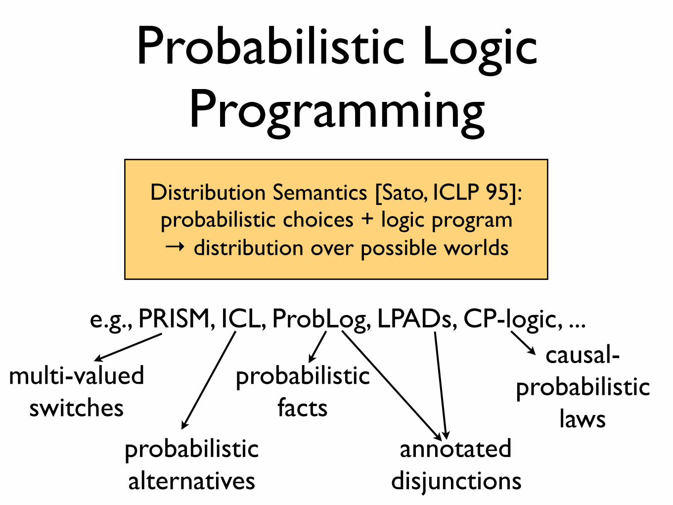
Probabilistic Logic Programming
Distribution Semantics [Sato, ICLP 95]:probabilistic choices + logic program→ distribution over possible worlds
e.g., PRISM, ICL, ProbLog, LPADs, CP-logic, ...
multi-valued switches
probabilistic alternatives
probabilistic facts
annotated disjunctions
causal-probabilistic
laws

Roadmap
• Modeling (ProbLog and Church, another representative of PP)
• Inference
• Learning
• Dynamics and Decisions
... with some detours on the way

ProbLog by example:
A bit of gambling h
• toss (biased) coin & draw ball from each urn
• win if (heads and a red ball) or (two balls of same color)
18

0.4 :: heads.
ProbLog by example:
A bit of gambling h
• toss (biased) coin & draw ball from each urn
• win if (heads and a red ball) or (two balls of same color)
probabilistic fact: heads is true with probability 0.4 (and false with 0.6)
18

0.4 :: heads.
0.3 :: col(1,red); 0.7 :: col(1,blue).
ProbLog by example:
A bit of gambling h
• toss (biased) coin & draw ball from each urn
• win if (heads and a red ball) or (two balls of same color)
annotated disjunction: first ball is red with probability 0.3 and blue with 0.7
18

0.4 :: heads.
0.3 :: col(1,red); 0.7 :: col(1,blue).0.2 :: col(2,red); 0.3 :: col(2,green); 0.5 :: col(2,blue).
annotated disjunction: second ball is red with probability 0.2, green with 0.3, and blue with 0.5
ProbLog by example:
A bit of gambling h
• toss (biased) coin & draw ball from each urn
• win if (heads and a red ball) or (two balls of same color)
18
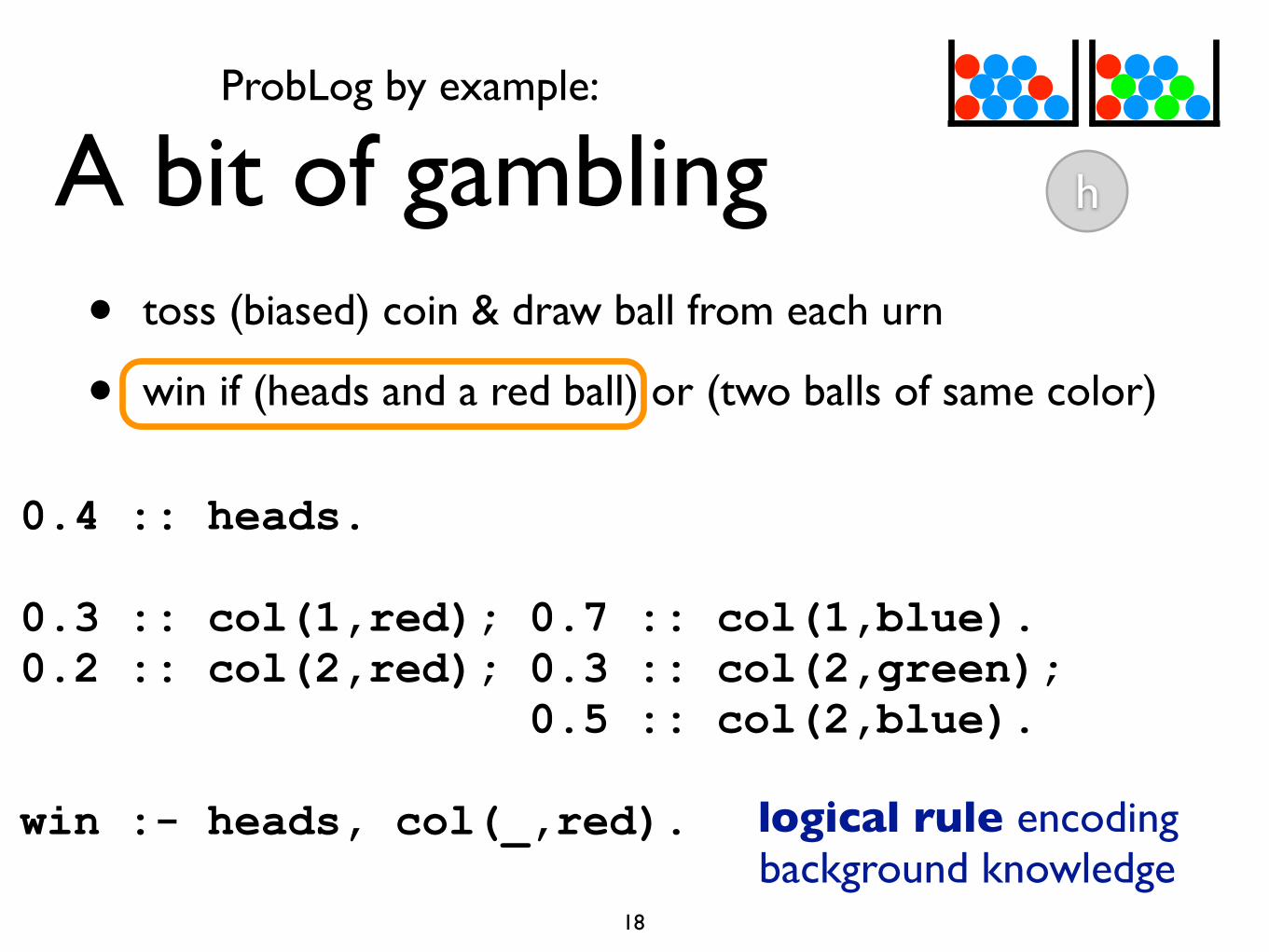
0.4 :: heads.
0.3 :: col(1,red); 0.7 :: col(1,blue).0.2 :: col(2,red); 0.3 :: col(2,green); 0.5 :: col(2,blue).
win :- heads, col(_,red). logical rule encoding background knowledge
ProbLog by example:
A bit of gambling h
• toss (biased) coin & draw ball from each urn
• win if (heads and a red ball) or (two balls of same color)
18

0.4 :: heads.
0.3 :: col(1,red); 0.7 :: col(1,blue).0.2 :: col(2,red); 0.3 :: col(2,green); 0.5 :: col(2,blue).
win :- heads, col(_,red).win :- col(1,C), col(2,C).
logical rule encoding background knowledge
ProbLog by example:
A bit of gambling h
• toss (biased) coin & draw ball from each urn
• win if (heads and a red ball) or (two balls of same color)
18

0.4 :: heads.
0.3 :: col(1,red); 0.7 :: col(1,blue).0.2 :: col(2,red); 0.3 :: col(2,green); 0.5 :: col(2,blue).
win :- heads, col(_,red).win :- col(1,C), col(2,C).
ProbLog by example:
A bit of gambling h
• toss (biased) coin & draw ball from each urn
• win if (heads and a red ball) or (two balls of same color)
probabilistic choices
consequences18

Questions
• Probability of win?
• Probability of win given col(2,green)?
• Most probable world where win is true?
0.4 :: heads.
0.3 :: col(1,red); 0.7 :: col(1,blue). 0.2 :: col(2,red); 0.3 :: col(2,green); 0.5 :: col(2,blue).
win :- heads, col(_,red). win :- col(1,C), col(2,C).
19

Questions
• Probability of win?
• Probability of win given col(2,green)?
• Most probable world where win is true?
0.4 :: heads.
0.3 :: col(1,red); 0.7 :: col(1,blue). 0.2 :: col(2,red); 0.3 :: col(2,green); 0.5 :: col(2,blue).
win :- heads, col(_,red). win :- col(1,C), col(2,C).
marginal probability
query
19

Questions
• Probability of win?
• Probability of win given col(2,green)?
• Most probable world where win is true?
0.4 :: heads.
0.3 :: col(1,red); 0.7 :: col(1,blue). 0.2 :: col(2,red); 0.3 :: col(2,green); 0.5 :: col(2,blue).
win :- heads, col(_,red). win :- col(1,C), col(2,C).
marginal probability
conditional probability
evidence
19

Questions
• Probability of win?
• Probability of win given col(2,green)?
• Most probable world where win is true?
0.4 :: heads.
0.3 :: col(1,red); 0.7 :: col(1,blue). 0.2 :: col(2,red); 0.3 :: col(2,green); 0.5 :: col(2,blue).
win :- heads, col(_,red). win :- col(1,C), col(2,C).
marginal probability
conditional probability
MPE inference
19

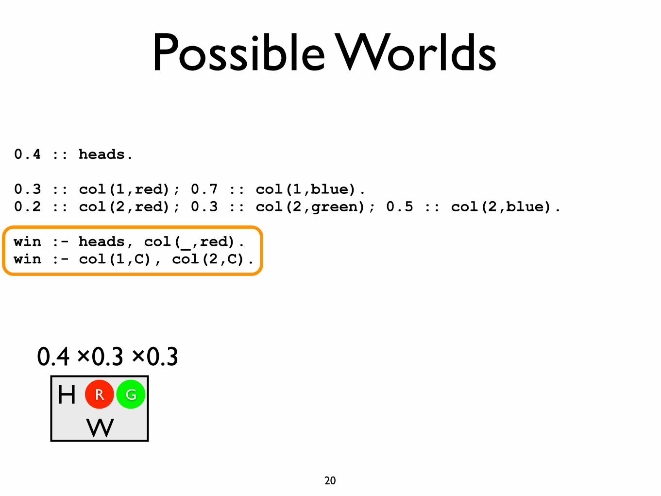
Possible Worlds
0.4 :: heads.
0.3 :: col(1,red); 0.7 :: col(1,blue). 0.2 :: col(2,red); 0.3 :: col(2,green); 0.5 :: col(2,blue).
win :- heads, col(_,red). win :- col(1,C), col(2,C).
20

Possible Worlds
0.4 :: heads.
0.3 :: col(1,red); 0.7 :: col(1,blue). 0.2 :: col(2,red); 0.3 :: col(2,green); 0.5 :: col(2,blue).
win :- heads, col(_,red). win :- col(1,C), col(2,C).
20
Possible Worlds
H
0.4 :: heads.
0.3 :: col(1,red); 0.7 :: col(1,blue). 0.2 :: col(2,red); 0.3 :: col(2,green); 0.5 :: col(2,blue).
win :- heads, col(_,red). win :- col(1,C), col(2,C).
0.4
20

Possible Worlds
H R
0.4 :: heads.
0.3 :: col(1,red); 0.7 :: col(1,blue). 0.2 :: col(2,red); 0.3 :: col(2,green); 0.5 :: col(2,blue).
win :- heads, col(_,red). win :- col(1,C), col(2,C).
×0.30.4
20

Possible Worlds
H R
×0.3
0.4 :: heads.
0.3 :: col(1,red); 0.7 :: col(1,blue). 0.2 :: col(2,red); 0.3 :: col(2,green); 0.5 :: col(2,blue).
win :- heads, col(_,red). win :- col(1,C), col(2,C).
×0.30.4G
20
Possible Worlds
HW
R
×0.3
0.4 :: heads.
0.3 :: col(1,red); 0.7 :: col(1,blue). 0.2 :: col(2,red); 0.3 :: col(2,green); 0.5 :: col(2,blue).
win :- heads, col(_,red). win :- col(1,C), col(2,C).
×0.30.4G
20

Possible Worlds
HW
R
×0.3
0.4 :: heads.
0.3 :: col(1,red); 0.7 :: col(1,blue). 0.2 :: col(2,red); 0.3 :: col(2,green); 0.5 :: col(2,blue).
win :- heads, col(_,red). win :- col(1,C), col(2,C).
×0.30.4G
20

All Possible Worlds
WR R
HW
R B
HW
R G
HW
R R
R G
R B HW
BB
H GB
HW
RB RB
GB
WBB
0.024
0.036
0.060
0.036
0.054
0.090
0.056 0.084
0.084 0.126
0.140 0.210
21
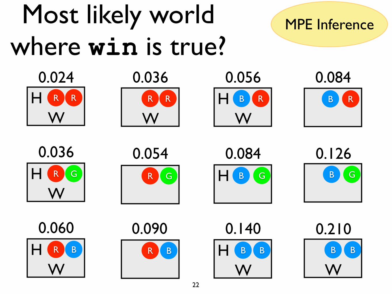
Most likely world where win is true?
WR R
HW
R B
HW
R G
HW
R R
R G
R B HW
BB
H GB
HW
RB RB
GB
WBB
0.024
0.036
0.060
0.036
0.054
0.090
0.056 0.084
0.084 0.126
0.140 0.210
MPE Inference
22

Most likely world where win is true?
WR R
HW
R B
HW
R G
HW
R R
R G
R B HW
BB
H GB
HW
RB RB
GB
WBB
0.024
0.036
0.060
0.036
0.054
0.090
0.056 0.084
0.084 0.126
0.140 0.210
MPE Inference
22

P(win)=
WR R
HW
R B
HW
R G
HW
R R
R G
R B HW
BB
H GB
HW
RB RB
GB
WBB
0.024
0.036
0.060
0.036
0.054
0.090
0.056 0.084
0.084 0.126
0.140 0.210
? Marginal Probability
23

P(win)=
WR R
HW
R B
HW
R G
HW
R R
R G
R B HW
BB
H GB
HW
RB RB
GB
WBB
0.024
0.036
0.060
0.036
0.054
0.090
0.056 0.084
0.084 0.126
0.140 0.210
∑ Marginal Probability
23

P(win)=
WR R
HW
R B
HW
R G
HW
R R
R G
R B HW
BB
H GB
HW
RB RB
GB
WBB
0.024
0.036
0.060
0.036
0.054
0.090
0.056 0.084
0.084 0.126
0.140 0.210
∑ =0.562 Marginal Probability
23

P(win|col(2,green))=
WR R
HW
R B
HW
R G
HW
R R
R G
R B HW
BB
H GB
HW
RB RB
GB
WBB
0.024
0.036
0.060
0.036
0.054
0.090
0.056 0.084
0.084 0.126
0.140 0.210
? Conditional Probability
24

=P(win∧col(2,green))/P(col(2,green))P(win|col(2,green))=
WR R
HW
R B
HW
R G
HW
R R
R G
R B HW
BB
H GB
HW
RB RB
GB
WBB
0.024
0.036
0.060
0.036
0.054
0.090
0.056 0.084
0.084 0.126
0.140 0.210
∑/∑ Conditional Probability
24

=P(win∧col(2,green))/P(col(2,green))P(win|col(2,green))=
WR R
HW
R B
HW
R G
HW
R R
R G
R B HW
BB
H GB
HW
RB RB
GB
WBB
0.024
0.036
0.060
0.036
0.054
0.090
0.056 0.084
0.084 0.126
0.140 0.210
∑/∑ Conditional Probability
24

P(win|col(2,green))==0.036/0.3=0.12
WR R
HW
R B
HW
R G
HW
R R
R G
R B HW
BB
H GB
HW
RB RB
GB
WBB
0.024
0.036
0.060
0.036
0.054
0.090
0.056 0.084
0.084 0.126
0.140 0.210
∑/∑ Conditional Probability
24

Alternative view: CP-Logic
25
[Vennekens et al, ICLP 04]
throws(john). 0.5::throws(mary).
0.8 :: break :- throws(mary). 0.6 :: break :- throws(john).
probabilistic causal laws
John throwsWindow breaks
Window breaks Window breaks
doesn’t break
doesn’t break doesn’t break
Mary throws Mary throwsdoesn’t throw doesn’t throw
1.0
0.6 0.4
0.50.50.5 0.5
0.80.80.20.2
P(break)=0.6×0.5×0.8+0.6×0.5×0.2+0.6×0.5+0.4×0.5×0.8

• Discrete- and continuous-valued random variables
Distributional Clauses (DC)
[Gutmann et al, TPLP 11; Nitti et al, IROS 13]26
Closely related to BLOG [Russell et al.]

• Discrete- and continuous-valued random variables
Distributional Clauses (DC)
length(Obj) ~ gaussian(6.0,0.45) :- type(Obj,glass).
[Gutmann et al, TPLP 11; Nitti et al, IROS 13]
random variable with Gaussian distribution
26
Closely related to BLOG [Russell et al.]

• Discrete- and continuous-valued random variables
Distributional Clauses (DC)
length(Obj) ~ gaussian(6.0,0.45) :- type(Obj,glass).stackable(OBot,OTop) :- ≃length(OBot) ≥ ≃length(OTop), ≃width(OBot) ≥ ≃width(OTop).
[Gutmann et al, TPLP 11; Nitti et al, IROS 13]
comparing values of random variables
26
Closely related to BLOG [Russell et al.]

• Discrete- and continuous-valued random variables
Distributional Clauses (DC)
length(Obj) ~ gaussian(6.0,0.45) :- type(Obj,glass).stackable(OBot,OTop) :- ≃length(OBot) ≥ ≃length(OTop), ≃width(OBot) ≥ ≃width(OTop).ontype(Obj,plate) ~ finite([0 : glass, 0.0024 : cup, 0 : pitcher, 0.8676 : plate, 0.0284 : bowl, 0 : serving, 0.1016 : none]) :- obj(Obj), on(Obj,O2), type(O2,plate).
[Gutmann et al, TPLP 11; Nitti et al, IROS 13]
random variable with discrete distribution
26
Closely related to BLOG [Russell et al.]

• Discrete- and continuous-valued random variables
Distributional Clauses (DC)
length(Obj) ~ gaussian(6.0,0.45) :- type(Obj,glass).stackable(OBot,OTop) :- ≃length(OBot) ≥ ≃length(OTop), ≃width(OBot) ≥ ≃width(OTop).ontype(Obj,plate) ~ finite([0 : glass, 0.0024 : cup, 0 : pitcher, 0.8676 : plate, 0.0284 : bowl, 0 : serving, 0.1016 : none]) :- obj(Obj), on(Obj,O2), type(O2,plate).
[Gutmann et al, TPLP 11; Nitti et al, IROS 13]26
Closely related to BLOG [Russell et al.]

• Defines a generative process (as for CP-logic)
• Logic programming variant of Blog
• Tree can become infinitely wide
• Sampling
• Well-defined under reasonable assumptions
27
Distributional Clauses (DC)

Dealing with uncertainty
Reasoning with relational data
Probabilistic Databases
Learning28
[Suciu et al 2011]

Dealing with uncertainty
relational database
Probabilistic Databases
Learning28
person city
ann london
bob york
eve new york
tom paris
bornIncity country
london uk
york uk
paris usa
cityIn
select x.person, y.country from bornIn x, cityIn y where x.city=y.city
[Suciu et al 2011]

Dealing with uncertainty
relational database
Probabilistic Databases
Learning
one world
28
person city
ann london
bob york
eve new york
tom paris
bornIncity country
london uk
york uk
paris usa
cityIn
select x.person, y.country from bornIn x, cityIn y where x.city=y.city
[Suciu et al 2011]

relational database
tuples as random variables
Probabilistic Databases
Learning
one world
28
person city
ann london
bob york
eve new york
tom paris
bornIncity country
london uk
york uk
paris usa
cityIn
person city P
ann london 0,87
bob york 0,95
eve new york 0,9
tom paris 0,56
bornIn
city country P
london uk 0,99
york uk 0,75
paris usa 0,4
cityIn
select x.person, y.country from bornIn x, cityIn y where x.city=y.city
[Suciu et al 2011]

relational database
tuples as random variables
Probabilistic Databases
Learning
one world
several possible worlds
28
person city
ann london
bob york
eve new york
tom paris
bornIncity country
london uk
york uk
paris usa
cityIn
person city P
ann london 0,87
bob york 0,95
eve new york 0,9
tom paris 0,56
bornIn
city country P
london uk 0,99
york uk 0,75
paris usa 0,4
cityIn
select x.person, y.country from bornIn x, cityIn y where x.city=y.city
probabilistic tables + database queries→ distribution over possible worlds
[Suciu et al 2011]

Example: Information Extraction
29 NELL: http://rtw.ml.cmu.edu/rtw/
instances for many different relations
degree of certainty

30
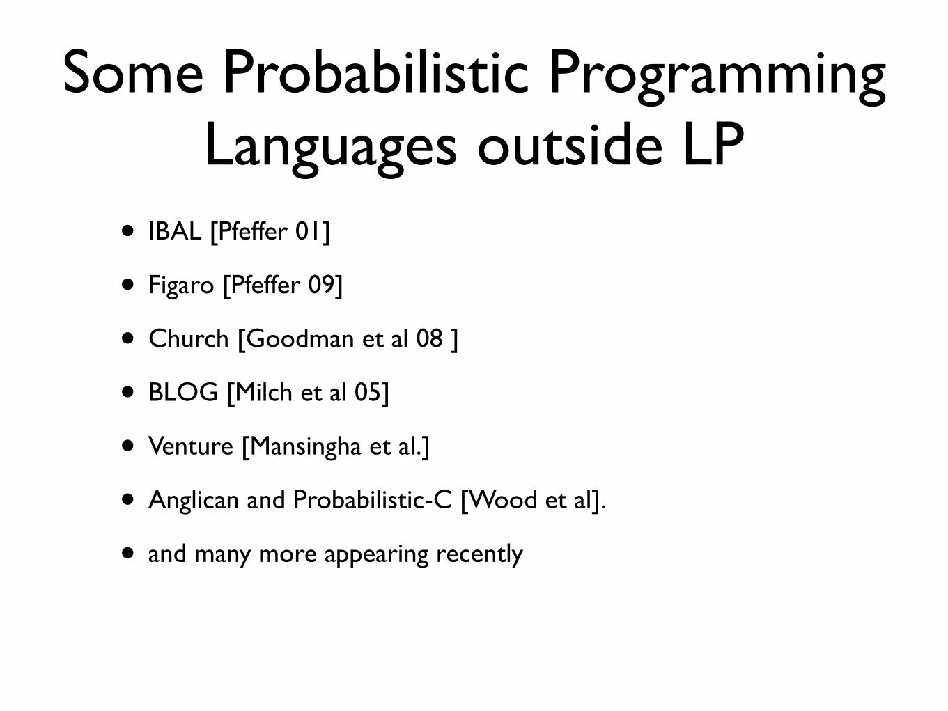
Some Probabilistic Programming Languages outside LP
• IBAL [Pfeffer 01]
• Figaro [Pfeffer 09]
• Church [Goodman et al 08 ]
• BLOG [Milch et al 05]
• Venture [Mansingha et al.]
• Anglican and Probabilistic-C [Wood et al].
• and many more appearing recently

(define win (or win1 win2))
(define heads (mem (lambda () (flip 0.4))))
Church by example:
A bit of gambling h
• toss (biased) coin & draw ball from each urn
• win if (heads and a red ball) or (two balls of same color)
32
(define color1 (mem (lambda () (if (flip 0.3) 'red 'blue))))
(define color2 (mem (lambda () (multinomial '(red green blue) '(0.2 0.3 0.5)))))
(define redball (or (equal? (color1) 'red) (equal? (color2) 'red)))
(define win1 (and (heads) redball))
(define win2 (equal? (color1) (color2)))

Probabilistic Programming Summary
• Church: functional programming + random primitives
• probabilistic generative model
• stochastic memoization
• sampling
• increasing number of probabilistic programming languages using various underlying paradigms
33

Roadmap
• Modeling (ProbLog and Church, another representative of PP)
• Inference
• Learning
• Dynamics and Decisions
... with some detours on the way

Answering Questions
program
queries
evidence
marginalprobabilities
conditionalprobabilities
MPE state
Given: Find:
?35

Answering Questions
program
queries
evidence
marginalprobabilities
conditionalprobabilities
MPE state
Given: Find:
?possible worlds
infeasi
ble
35

Answering Questions
program
queries
evidence
marginalprobabilities
conditionalprobabilities
MPE state
Given: Find:
?possible worlds
infeasi
blelogical reasoning
probabilistic inference
data structure
35

Answering Questions
program
queries
evidence
marginalprobabilities
conditionalprobabilities
MPE state
Given: Find:
?possible worlds
infeasi
blelogical reasoning
probabilistic inference
data structure
35
knowledge compilation

Answering Questions
program
queries
evidence
marginalprobabilities
conditionalprobabilities
MPE state
Given: Find:
?possible worlds
infeasi
blelogical reasoning
probabilistic inference
data structure
1. using proofs2. using models
35
knowledge compilation

Proofs in ProbLog
0.8::stress(ann). 0.6::influences(ann,bob). 0.2::influences(bob,carl).
smokes(X) :- stress(X). smokes(X) :- influences(Y,X), smokes(Y).
influences(bob,carl)&influences(ann,bob)&stress(ann)
?- smokes(carl).
?- stress(carl). ?- influences(Y,carl),smokes(Y).
?- smokes(bob).
?- stress(bob). ?- influences(Y1,bob),smokes(Y1).
?- smokes(ann).
?- influences(Y2,ann),smokes(Y2).?- stress(ann).
Y=bob
Y1=ann
probability of proof = 0.2 × 0.6 × 0.8 = 0.09636
influences(bob,carl) & influences(ann,bob)
& stress(ann)
Proofs in ProbLog
0.8::stress(ann). 0.4::stress(bob). 0.6::influences(ann,bob). 0.2::influences(bob,carl).
smokes(X) :- stress(X). smokes(X) :- influences(Y,X), smokes(Y).
?- smokes(carl).
?- stress(carl). ?- influences(Y,carl),smokes(Y).
?- smokes(bob).
?- stress(bob). ?- influences(Y1,bob),smokes(Y1).
?- smokes(ann).
?- influences(Y2,ann),smokes(Y2).?- stress(ann).
Y=bob
Y1=ann
0.2×0.6×0.8 = 0.096
37

influences(bob,carl) & influences(ann,bob)
& stress(ann)
Proofs in ProbLog
0.8::stress(ann). 0.4::stress(bob). 0.6::influences(ann,bob). 0.2::influences(bob,carl).
smokes(X) :- stress(X). smokes(X) :- influences(Y,X), smokes(Y).
?- smokes(carl).
?- stress(carl). ?- influences(Y,carl),smokes(Y).
?- smokes(bob).
?- stress(bob). ?- influences(Y1,bob),smokes(Y1).
?- smokes(ann).
?- influences(Y2,ann),smokes(Y2).?- stress(ann).
Y=bob
Y1=anninfluences(bob,carl) & stress(bob)
0.2×0.6×0.8 = 0.096
0.2×0.4 = 0.08
proofs overlap! cannot sum probabilities (disjoint-sum-problem)
37

infl(bob,carl) & infl(ann,bob) & st(ann) & \+st(bob)
infl(bob,carl) & infl(ann,bob) & st(ann) & st(bob)
infl(bob,carl) & \+infl(ann,bob) & st(ann) & st(bob)
infl(bob,carl) & infl(ann,bob) & \+st(ann) & st(bob)
infl(bob,carl) & \+infl(ann,bob) & \+st(ann) & st(bob)
...
Disjoint-Sum-Problempossible worlds
38

infl(bob,carl) & infl(ann,bob) & st(ann) & \+st(bob)
infl(bob,carl) & infl(ann,bob) & st(ann) & st(bob)
infl(bob,carl) & \+infl(ann,bob) & st(ann) & st(bob)
infl(bob,carl) & infl(ann,bob) & \+st(ann) & st(bob)
infl(bob,carl) & \+infl(ann,bob) & \+st(ann) & st(bob)
...
Disjoint-Sum-Probleminfluences(bob,carl) &
influences(ann,bob) & stress(ann)
possible worlds
38

infl(bob,carl) & infl(ann,bob) & st(ann) & \+st(bob)
infl(bob,carl) & infl(ann,bob) & st(ann) & st(bob)
infl(bob,carl) & \+infl(ann,bob) & st(ann) & st(bob)
infl(bob,carl) & infl(ann,bob) & \+st(ann) & st(bob)
infl(bob,carl) & \+infl(ann,bob) & \+st(ann) & st(bob)
...
Disjoint-Sum-Problem
influences(bob,carl) & stress(bob)
influences(bob,carl) & influences(ann,bob) & stress(ann)
possible worlds
sum of proof probabilities: 0.096+0.08 = 0.176038

infl(bob,carl) & infl(ann,bob) & st(ann) & \+st(bob)
infl(bob,carl) & infl(ann,bob) & st(ann) & st(bob)
infl(bob,carl) & \+infl(ann,bob) & st(ann) & st(bob)
infl(bob,carl) & infl(ann,bob) & \+st(ann) & st(bob)
infl(bob,carl) & \+infl(ann,bob) & \+st(ann) & st(bob)
...
Disjoint-Sum-Problem
influences(bob,carl) & stress(bob)
influences(bob,carl) & influences(ann,bob) & stress(ann)
possible worlds
sum of proof probabilities: 0.096+0.08 = 0.1760
0.05760.03840.02560.00960.0064
∑ = 0.1376
38

infl(bob,carl) & infl(ann,bob) & st(ann) & \+st(bob)
infl(bob,carl) & infl(ann,bob) & st(ann) & st(bob)
infl(bob,carl) & \+infl(ann,bob) & st(ann) & st(bob)
infl(bob,carl) & infl(ann,bob) & \+st(ann) & st(bob)
infl(bob,carl) & \+infl(ann,bob) & \+st(ann) & st(bob)
...
Disjoint-Sum-Problem
influences(bob,carl) & stress(bob)
influences(bob,carl) & influences(ann,bob) & stress(ann)
possible worlds
sum of proof probabilities: 0.096+0.08 = 0.1760
0.05760.03840.02560.00960.0064
∑ = 0.1376
38
solution: knowledge compilation

Binary Decision Diagrams
i(b,c)
0 1
i(a,b)
s(a)
s(b)
influences(bob,carl) & influences(ann,bob) & stress(ann)
influences(bob,carl) & stress(bob)
• compact graphical representation of Boolean formula
• automatically disjoins proofs
• popular in many branches of CS
[Bryant 86]
39 & not stress(bob)

Markov Chain Monte Carlo (MCMC)
• Generate next sample by modifying current one
• Most common inference approach for PP languages such as Church, BLOG, ...
• Also considered for PRISM and ProbLog
Key challenges: - how to propose next sample- how to handle evidence
40

Roadmap
• Modeling (ProbLog and Church, another representative of PP)
• Inference
• Learning
• Dynamics and Decisions
... with some detours on the way

Parameter Learning
class(Page,C) :- has_word(Page,W), word_class(W,C).
class(Page,C) :- links_to(OtherPage,Page), class(OtherPage,OtherClass),
link_class(OtherPage,Page,OtherClass,C).
for each CLASS1, CLASS2 and each WORD
?? :: link_class(Source,Target,CLASS1,CLASS2).?? :: word_class(WORD,CLASS).
42
e.g., webpage classification model

Sampling Interpretations
43

Sampling Interpretations
43

Parameter Estimation
44

Parameter Estimation
44
p(fact) = count(fact is true) Number of interpretations

Learning from partial interpretations
• Not all facts observed
• Soft-EM
• use expected count instead of count
• P(Q |E) -- conditional queries !
45 [Gutmann et al, ECML 11; Fierens et al, TPLP 14]

Rule learning — NELL
16 Luc De Raedt, Anton Dries, Ingo Thon, Guy Van den Broeck, Mathias Verbeke
6.1 Dataset
In order to test probabilistic rule learning for facts extracted by NELL, we used the NELL athletedataset8, which has already been used in the context of meta-interpretive learning of higher-orderdyadic Datalog [36]. This dataset contains 10130 facts. The number of facts per predicate is listedin Table 5. The unary predicates in this dataset are deterministic, whereas the binary predicateshave a probability attached9.
Table 5: Number of facts per predicate (NELL athlete dataset)
athletecoach(person,person) 18 athleteplaysforteam(person,team) 721athleteplayssport(person,sport) 1921 teamplaysinleague(team,league) 1085
athleteplaysinleague(person,league) 872 athletealsoknownas(person,name) 17coachesinleague(person,league) 93 coachesteam(person,team) 132
teamhomestadium(team,stadium) 198 teamplayssport(team,sport) 359athleteplayssportsteamposition(person,position) 255 athletehomestadium(person,stadium) 187
athlete(person) 1909 attraction(stadium) 2coach(person) 624 female(person) 2male(person) 7 hobby(sport) 5
organization(league) 1 person(person) 2personafrica(person) 1 personasia(person) 4
personaustralia(person) 22 personcanada(person) 1personeurope(person) 1 personmexico(person) 108
personus(person) 6 sport(sport) 36sportsleague(league) 18 sportsteam(team) 1330
sportsteamposition(position) 22 stadiumoreventvenue(stadium) 171
Table 5 also shows the types that were used for the variables in the base declarations for thepredicates. As indicated in Section 4.5, this typing of the variables forms a syntactic restrictionon the possible groundings and ensures that arguments are only instantiated with variables of theappropriate type. Furthermore, the LearnRule function of the ProbFOIL algorithm is based onmFOIL and allows to incorporate a number of variable constraints. To reduce the search space, weimposed that unary predicates that are added to a candidate rule during the learning process canonly use variables that have already been introduced. Binary predicates can introduce at most onenew variable.
6.2 Relational probabilistic rule learning
In order to illustrate relational probabilistic rule learning with ProbFOIL+ in the context of NELL,we will learn rules and report their respective accuracy for each binary predicate with more then500 facts. In order to show ProbFOIL+’s speed, also the runtimes are reported. Unless indicatedotherwise, both the m-estimate’s m value and the beam width were set to 1. The value of p forrule significance was set to 0.9. The rules are postprocessed such that only range-restricted rulesare obtained. Furthermore, to avoid a bias towards to majority class, the examples are balanced,i.e., negative examples are added to balance the number of positives. Anton: negative examplesare removed?
8 Kindly provided by Tom Mitchell and Jayant Krishnamurthy (CMU).9 The dataset in ProbFOIL+ format can be downloaded from [removed for double-blind review].
Adaptation of standard rule learning and inductive logic programming setting
[De Raedt et al IJCAI 15]

Experiments

Roadmap
• Modeling (ProbLog and Church, another representative of PP)
• Inference
• Learning
• Dynamics and Decisions
... with some detours on the way

07/14/10 DTProbLog 17
HomerMarge
Bart Lisa
Lenny
Apu
Moe
SeymourRalph
Maggie
????
??
?? ??
??
??
??
??
??
+$5
-$3
Which strategy gives the maximum expected utility?
Viral MarketingWhich advertising strategy maximizes
expected profit?
[Van den Broeck et al, AAAI 10]49

07/14/10 DTProbLog 17
HomerMarge
Bart Lisa
Lenny
Apu
Moe
SeymourRalph
Maggie
????
??
?? ??
??
??
??
??
??
+$5
-$3
Which strategy gives the maximum expected utility?
Viral Marketing
[Van den Broeck et al, AAAI 10]
decide truth values of some atoms
49

DTProbLog1
23
4
person(1). person(2). person(3). person(4).
friend(1,2). friend(2,1). friend(2,4). friend(3,4). friend(4,2).
50

DTProbLog? :: marketed(P) :- person(P).
decision fact: true or false?
1
23
4
person(1). person(2). person(3). person(4).
friend(1,2). friend(2,1). friend(2,4). friend(3,4). friend(4,2).
50

DTProbLog? :: marketed(P) :- person(P).
0.3 :: buy_trust(X,Y) :- friend(X,Y). 0.2 :: buy_marketing(P) :- person(P). buys(X) :- friend(X,Y), buys(Y), buy_trust(X,Y).buys(X) :- marketed(X), buy_marketing(X).
probabilistic facts + logical rules
1
23
4
person(1). person(2). person(3). person(4).
friend(1,2). friend(2,1). friend(2,4). friend(3,4). friend(4,2).
50

DTProbLog? :: marketed(P) :- person(P).
0.3 :: buy_trust(X,Y) :- friend(X,Y). 0.2 :: buy_marketing(P) :- person(P). buys(X) :- friend(X,Y), buys(Y), buy_trust(X,Y).buys(X) :- marketed(X), buy_marketing(X).
buys(P) => 5 :- person(P). marketed(P) => -3 :- person(P).
utility facts: cost/reward if true
1
23
4
person(1). person(2). person(3). person(4).
friend(1,2). friend(2,1). friend(2,4). friend(3,4). friend(4,2).
50

DTProbLog? :: marketed(P) :- person(P).
0.3 :: buy_trust(X,Y) :- friend(X,Y). 0.2 :: buy_marketing(P) :- person(P). buys(X) :- friend(X,Y), buys(Y), buy_trust(X,Y).buys(X) :- marketed(X), buy_marketing(X).
buys(P) => 5 :- person(P). marketed(P) => -3 :- person(P).
1
23
4
person(1). person(2). person(3). person(4).
friend(1,2). friend(2,1). friend(2,4). friend(3,4). friend(4,2).
marketed(1) marketed(3)
bt(2,1) bt(2,4) bm(1)
buys(1) buys(2)
utility = −3 + −3 + 5 + 5 = 4 probability = 0.0032
world contributes 0.0032×4 to
expected utility of strategy
50

DTProbLog? :: marketed(P) :- person(P).
0.3 :: buy_trust(X,Y) :- friend(X,Y). 0.2 :: buy_marketing(P) :- person(P). buys(X) :- friend(X,Y), buys(Y), buy_trust(X,Y).buys(X) :- marketed(X), buy_marketing(X).
buys(P) => 5 :- person(P). marketed(P) => -3 :- person(P).
1
23
4
person(1). person(2). person(3). person(4).
friend(1,2). friend(2,1). friend(2,4). friend(3,4). friend(4,2).
task: find strategy that maximizes expected utilitysolution: using ProbLog technology
50

Phenetic
l Causes: Mutations l All related to similar
phenotype l Effects: Differentially expressed genes l 27 000 cause effect pairs
l Interaction network: l 3063 nodes
l Genes l Proteins
l 16794 edges l Molecular interactions l Uncertain
l Goal: connect causes to effects through common subnetwork
l = Find mechanism l Techniques:
l DTProbLog [Van den Broeck] l Approximate inference
[De Maeyer et al., Molecular Biosystems 13, NAR 15]
51Can we find the mechanism connecting causes to effects?
DT-ProbLogdecision theoretic version

Distributional Clauses (DC)
● A probabilistic logic language
● Logic (relational): a template to define random variables
● MDP representation in Dynamic DC:
– Transition model: Headt+1~ Distribution ← Conditionst
– Applicable actions: applicable(Action)t ← Conditionst
– Reward: reward(R)t ← Conditionst
– Terminal state: stopt ← Conditionst
● The state can contain:
– Discrete, continuous variables
– The number of variables in the state can change over time

53
IROS 13

53
IROS 13

Learning relational affordancesLearn probabilistic model
From two object interactions Generalize to N
Shelf
push
Shelftap
Shelf
grasp
Moldovan et al. ICRA 12, 13, 14, PhD 15

Learning relational affordancesLearn probabilistic model
From two object interactions Generalize to N
Shelf
push
Shelftap
Shelf
grasp
Moldovan et al. ICRA 12, 13, 14, PhD 15

What is an affordance ?
(a) Disparity image (b) Segmented image with landmark points
Clip 7: Illustration of the object size computation. Left-hand image shows the disparity mapof the example shown in Figure 5. The orange points in the right-hand image show the pointsthat intersect with the ellipse’s major axis. The orange points are mapped onto 3D using theirassociated disparity value, and the 3D distance between each pair is defined as the object size.
To learn an a↵ordance model, the robot first performs a behavioural babblingstage, in which it explores the e↵ect of its actions on the environment. Forthis behavioural babbling stage, for the single-arm actions the robot uses itsright-arm only. For these actions a model of the left-arm will be later built byexploiting symmetry as in [3]. We include the simultaneous two-arm push onthe same object in the babbling phase, allowing for a more accurate modellingof action e↵ects for the iCub.4
The babbling phase consists of placing pairs of objects in front of the robotat various positions. The robot executes one of its actions A described above onone object (named: main object, OMain). OMain may interact with the otherobject (secondary object, OSec) causing it to also move. Figure 8 shows sucha setting, with the objects’ position before (l) and after (r) a right-arm action(tap(10)) execution.
Clip 8: Relational O before (l), and E after the action execution (r).
4As opposed to the two-arm a↵ordance modelling in [3], we also include in the babblingphase the two-arm simultaneous actions whose e↵ects might not always be well modelled bythe sum of the individual single-arm actions.
15
• Formalism — related to STRIPS but models delta
• but also joint probability model over A, E, O
During this behavioural babbling stage, data for O, A and E are collected foreach of the robot’s exploratory actions. The robot executed 150 such exploratoryactions. One example of collected data during such an action is shown in Table 1.Note that these values are obtained by the robot from its perception, whichnaturally introduces uncertainty, which the relational a↵ordance model takesinto account (e.g., the displacement of OMain is observed to be a bit more than10cm).
Table 1: Example collected O, A, E data for action in Figure 8
Object Properties Action E↵ectsshapeOMain : sprismshapeOSec : sprism
distXOMain,OSec : 6.94cmdistYOMain,OSec : 1.90cm
tap(10)
displXOMain : 10.33cmdisplYOMain : �0.68cmdisplXOSec : 7.43cmdisplYOSec : �1.31cm
During the babbling phase, we also learn the action space of each action. Asthe iCub is not mobile, and each arm has a specific action range, each ai 2 Acan be performed when an object is located in a specific action space. An objectcan be acted upon by both arms, by one arm but not the other, or it can becompletely out of the reach of the robot. If the exploratory arm action on anobject fails because no inverse kinematics solution was found, then that object isnot in that arm’s action space. We will show later how any spatial constraints,such as action space, can be modelled with logical rules.
5.2. Learning the Model
The model will be learnt from the data collected during the robot’s 150exploratory actions, one instance of such data as illustrated in Table 1. Wewill model the (relational) object properties: distX, distY (the x and y-axisdistance between the centroids of the two objects), and the e↵ects: displX anddisplY (the x and y-axis displacement of an object) with continuous distributionrandom variables. We will start by learning a Linear Conditional Gaussian(LCG) Bayesian Network [26]. An LCG BN specifies a distribution over amixture of discrete and continuous variables. In an LCG, a discrete randomvariable may have only discrete parents, while a continuous random variable mayhave both discrete and continuous parents. A continuous random variable (X)will have a single Gaussian distribution function whose mean depends linearlyon the state of its continuous parent variables (Y ) for each configuration of itsdiscrete parent variables (U) [26]. This LCG distribution can be representedas: P (X = x|Y = y, U = u) = N (x|M(u) +W (u)T y,�2(u)), with M a table ofmean values, W a table of regression (weight) coe�cient vectors, and � a tableof variances (independent of Y ). [26]
To learn an LCG BN for our setting, we will approximate displX, displY ,and distX and distY by conditional Gaussian distributions over the short dis-tances over which objects interact. These distances will be enforced by addinglogical rules.
16

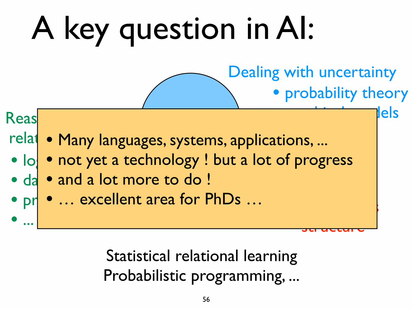
A key question in AI:Dealing with uncertainty
Reasoning with relational data
Learning
Statistical relational learningProbabilistic programming, ...
?• logic• databases• programming• ...
• probability theory• graphical models• ...
• parameters• structure
56
A key question in AI:Dealing with uncertainty
Reasoning with relational data
Learning
Statistical relational learningProbabilistic programming, ...
?• logic• databases• programming• ...
• probability theory• graphical models• ...
• parameters• structure
56
• Many languages, systems, applications, ...• not yet a technology ! but a lot of progress• and a lot more to do !• … excellent area for PhDs …

Thanks!
http://dtai.cs.kuleuven.be/problog
Maurice BruynoogheBart DemoenAnton Dries Daan FierensJason Filippou
Bernd GutmannManfred JaegerGerda Janssens
Kristian KerstingAngelika Kimmig
Theofrastos MantadelisWannes Meert
Bogdan Moldovan Siegfried Nijssen
Davide Nitti Joris Renkens
Kate RevoredoRicardo Rocha
Vitor Santos CostaDimitar Shterionov
Ingo Thon Hannu Toivonen
Guy Van den Broeck Mathias Verbeke Jonas Vlasselaer
57
Thanks !