probabilistic bias analysis of epidemiological results - · pdf fileprobabilistic bias...
TRANSCRIPT
1
Probabilistic bias analysis of epidemiological results
Nicola Orsini
Division of Nutritional Epidemiology, The National Institute of Environmental Medicine,
Karolinska Institutet
Second Nordic and Baltic countries Stata Users Group meeting
Stockholm, 7 September, 2007
2
Outline
• Background of the methods • Application to epidemiology
• Deterministic sensitivity analysis
• Probabilistic sensitivity analysis • Strengths and limitations

3
Background
Sensitivity analysis is the study of how the variation in the output of a model can be attributed to different sources of variation. Methods dealing with uncertainty in model outputs are well known in • Decision modeling • Risk analysis
and applied in a variety of industries and applications
Engineering Financial Planning Project Management Government
Health Care Pharmaceuticals Consulting Insurance
4
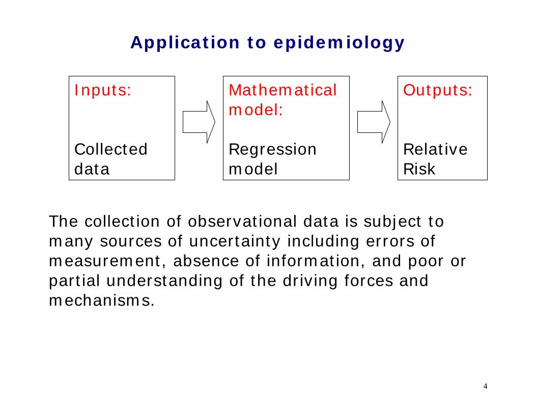
Application to epidemiology
The collection of observational data is subject to many sources of uncertainty including errors of measurement, absence of information, and poor or partial understanding of the driving forces and mechanisms.
Mathematical model: Regression model
Inputs: Collected data
Outputs: Relative Risk
5
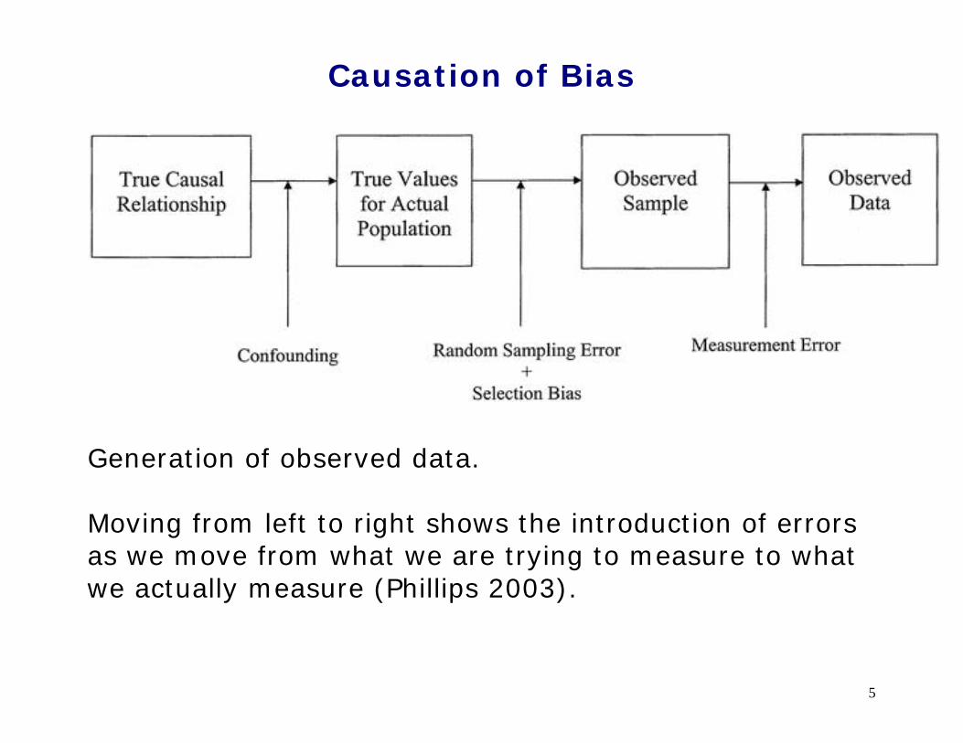
Causation of Bias
Generation of observed data. Moving from left to right shows the introduction of errors as we move from what we are trying to measure to what we actually measure (Phillips 2003).
6
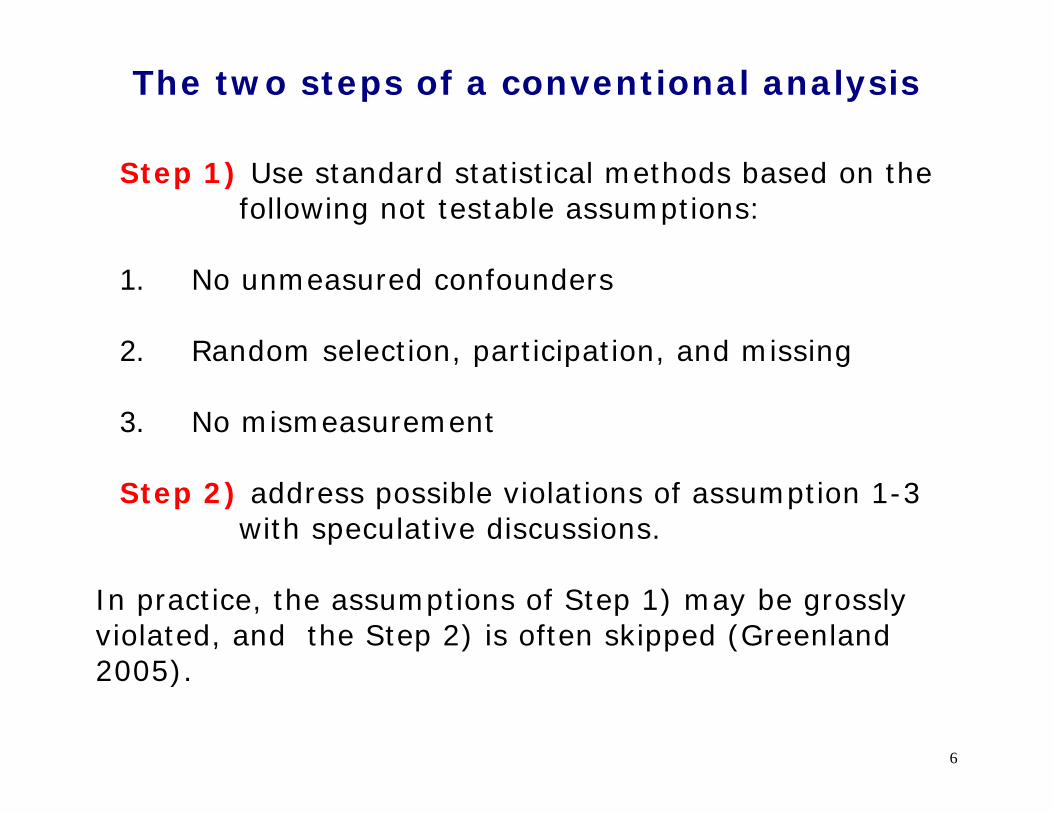
The two steps of a conventional analysis
Step 1) Use standard statistical methods based on the following not testable assumptions:
1. No unmeasured confounders
2. Random selection, participation, and missing
3. No mismeasurement
Step 2) address possible violations of assumption 1-3
with speculative discussions.
In practice, the assumptions of Step 1) may be grossly violated, and the Step 2) is often skipped (Greenland 2005).
7
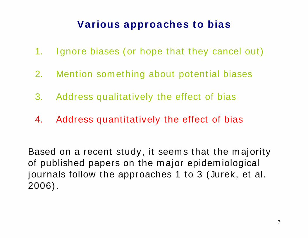
Various approaches to bias
1. Ignore biases (or hope that they cancel out)
2. Mention something about potential biases
3. Address qualitatively the effect of bias
4. Address quantitatively the effect of bias Based on a recent study, it seems that the majority of published papers on the major epidemiological journals follow the approaches 1 to 3 (Jurek, et al. 2006).

8
Why quantitative methods are rarely used?
1. Lack of training in epidemiology and biostatistics courses
2. No request from the reviewers
3. Lack of user-friendly packaged software
9
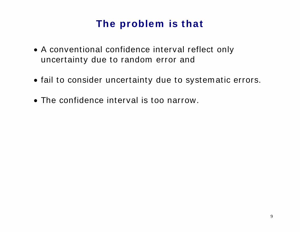
The problem is that
• A conventional confidence interval reflect only uncertainty due to random error and
• fail to consider uncertainty due to systematic errors.
• The confidence interval is too narrow.
10
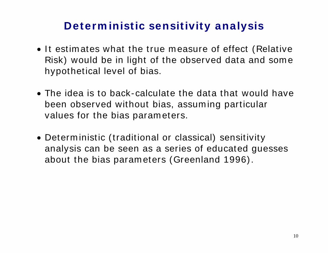
Deterministic sensitivity analysis • It estimates what the true measure of effect (Relative
Risk) would be in light of the observed data and some hypothetical level of bias.
• The idea is to back-calculate the data that would have
been observed without bias, assuming particular values for the bias parameters.
• Deterministic (traditional or classical) sensitivity
analysis can be seen as a series of educated guesses about the bias parameters (Greenland 1996).
11
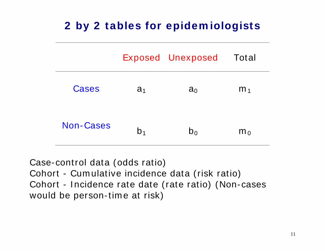
2 by 2 tables for epidemiologists
Exposed Unexposed Total
Cases
a1 a0 m1
Non-Cases
b1 b0 m0
Case-control data (odds ratio) Cohort - Cumulative incidence data (risk ratio) Cohort - Incidence rate date (rate ratio) (Non-cases would be person-time at risk)
12
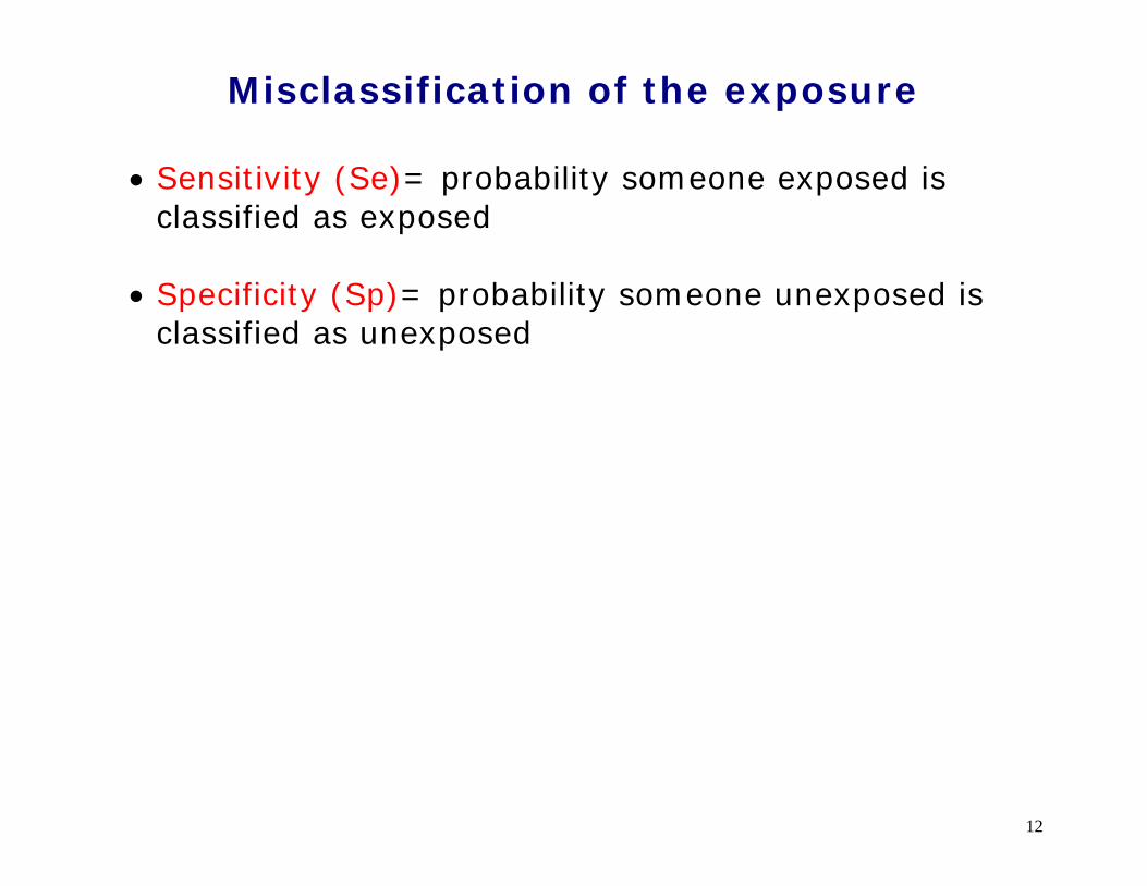
Misclassification of the exposure
• Sensitivity (Se)= probability someone exposed is classified as exposed
• Specificity (Sp)= probability someone unexposed is
classified as unexposed
13
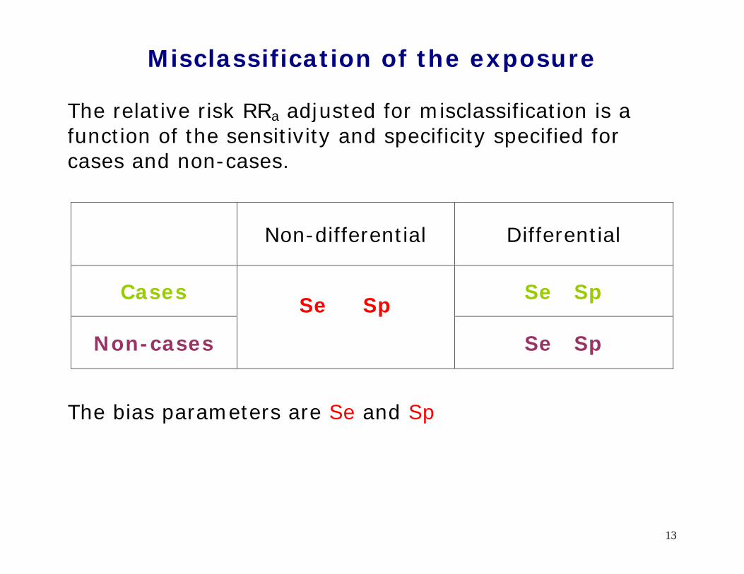
Misclassification of the exposure The relative risk RRa adjusted for misclassification is a function of the sensitivity and specificity specified for cases and non-cases.
Non-differential Differential
Cases Se Sp
Non-cases
Se Sp
Se Sp
The bias parameters are Se and Sp

14
Misclassification of the exposure
RRa = RRo / K
K = function(Se, Sp) RRa is the misclassified-adjusted relative risk RRo is the observed relative risk
K is a factor that govern magnitude and direction of bias. If Se = Sp = 1 there is no misclassification.
15
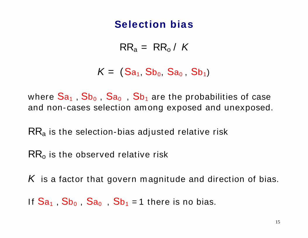
Selection bias
RRa = RRo / K
K = (Sa1, Sb0, Sa0 , Sb1) where Sa1 , Sb0 , Sa0 , Sb1 are the probabilities of case and non-cases selection among exposed and unexposed. RRa is the selection-bias adjusted relative risk RRo is the observed relative risk
K is a factor that govern magnitude and direction of bias. If Sa1 , Sb0 , Sa0 , Sb1 =1 there is no bias.

16
Unmeasured or uncontrolled confounder
A confounder is associated with the exposure and is also an independent risk factor of the disease outcome. If either association is non-existent, there is no confounding. The bias parameters are Pc1 , Pc0 , and RRcd
Disease Outcome
Confounder
Exposure
Pc1 = Prevalence of the confounder among the exposed Pc0 = Prevalence of the confounder among the unexposed
RRcd = confounder-disease relative risk

17
Unmeasured or uncontrolled confounder
RRa = RRo / K
K = (Pc0, Pc1 , RRcd ) RRa is the confounder-adjusted relative risk RRo is the observed relative risk
K is a factor that govern magnitude and direction of bias If Pc1 = Pc0 there is no confounding If RRcd = 1 there is no confounding
18
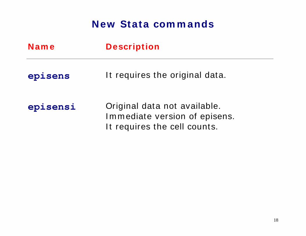
New Stata commands Name Description
episens
It requires the original data.
episensi
Original data not available. Immediate version of episens. It requires the cell counts.
19
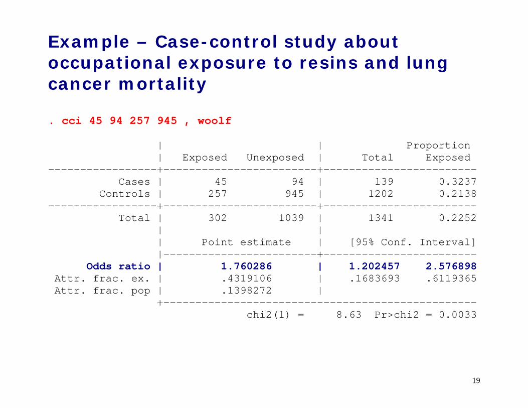
Example – Case-control study about occupational exposure to resins and lung cancer mortality
. cci 45 94 257 945 , woolf | | Proportion | Exposed Unexposed | Total Exposed -----------------+------------------------+------------------------ Cases | 45 94 | 139 0.3237 Controls | 257 945 | 1202 0.2138 -----------------+------------------------+------------------------ Total | 302 1039 | 1341 0.2252 | | | Point estimate | [95% Conf. Interval] |------------------------+------------------------ Odds ratio | 1.760286 | 1.202457 2.576898 Attr. frac. ex. | .4319106 | .1683693 .6119365 Attr. frac. pop | .1398272 | +------------------------------------------------- chi2(1) = 8.63 Pr>chi2 = 0.0033

20
Non-differential misclassification of the exposure . episensi 45 94 257 945 , st(cc) dseca(c(.9)) dspca(c(.9)) /// dsenc(c(.9)) dspnc(c(.9)) Se|Cases : Constant(.9) Sp|Cases : Constant(.9) Se|No-Cases: Constant(.9) Sp|No-Cases: Constant(.9) Observed Odds Ratio [95% Conf. Interval]= 1.76 [1.20, 2.58] Deterministic sensitivity analysis for misclassification of the exposure External adjusted Odds Ratio = 2.34 Percent bias = -25%

21
Differential misclassification of the exposure . episensi 45 94 257 945, st(cc) dseca(c(.9)) dspca(c(.8)) /// dsenc(c(.8)) dspnc(c(.8)) Se|Cases : Constant(.9) Sp|Cases : Constant(.8) Se|No-Cases: Constant(.8) Sp|No-Cases: Constant(.8) Observed Odds Ratio [95% Conf. Interval]= 1.76 [1.20, 2.58] Deterministic sensitivity analysis for misclassification of the exposure External adjusted Odds Ratio = 9.11 Percent bias = -81%
22
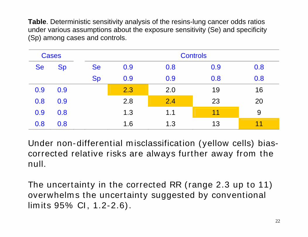
Table. Deterministic sensitivity analysis of the resins-lung cancer odds ratios under various assumptions about the exposure sensitivity (Se) and specificity (Sp) among cases and controls.
Cases Controls Se Sp Se 0.9 0.8 0.9 0.8
Sp 0.9 0.9 0.8 0.8 0.9 0.9 2.3 2.0 19 16 0.8 0.9 2.8 2.4 23 20 0.9 0.8 1.3 1.1 11 9 0.8 0.8 1.6 1.3 13 11
Under non-differential misclassification (yellow cells) bias-corrected relative risks are always further away from the null. The uncertainty in the corrected RR (range 2.3 up to 11) overwhelms the uncertainty suggested by conventional limits 95% CI, 1.2-2.6).
23
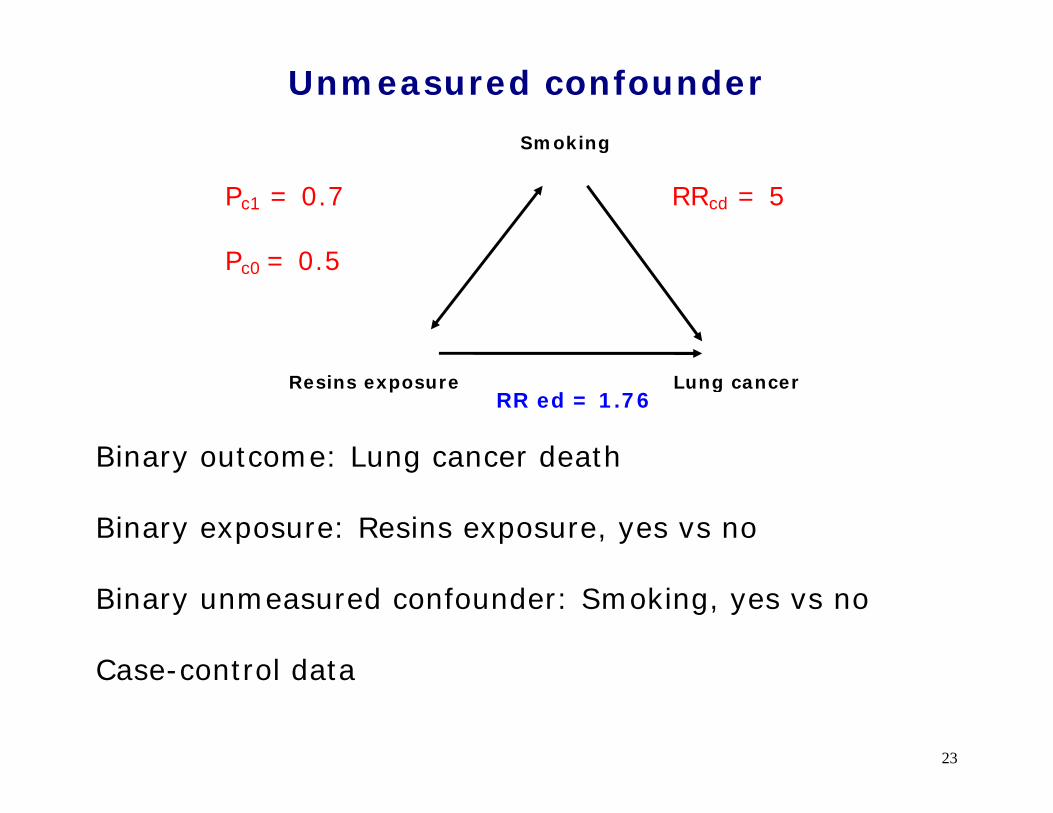
Unmeasured confounder
Binary outcome: Lung cancer death Binary exposure: Resins exposure, yes vs no Binary unmeasured confounder: Smoking, yes vs no Case-control data
Lung cancer Resins exposure
Pc1 = 0.7 Pc0 = 0.5
Smoking
RRcd = 5
RR ed = 1.76
24
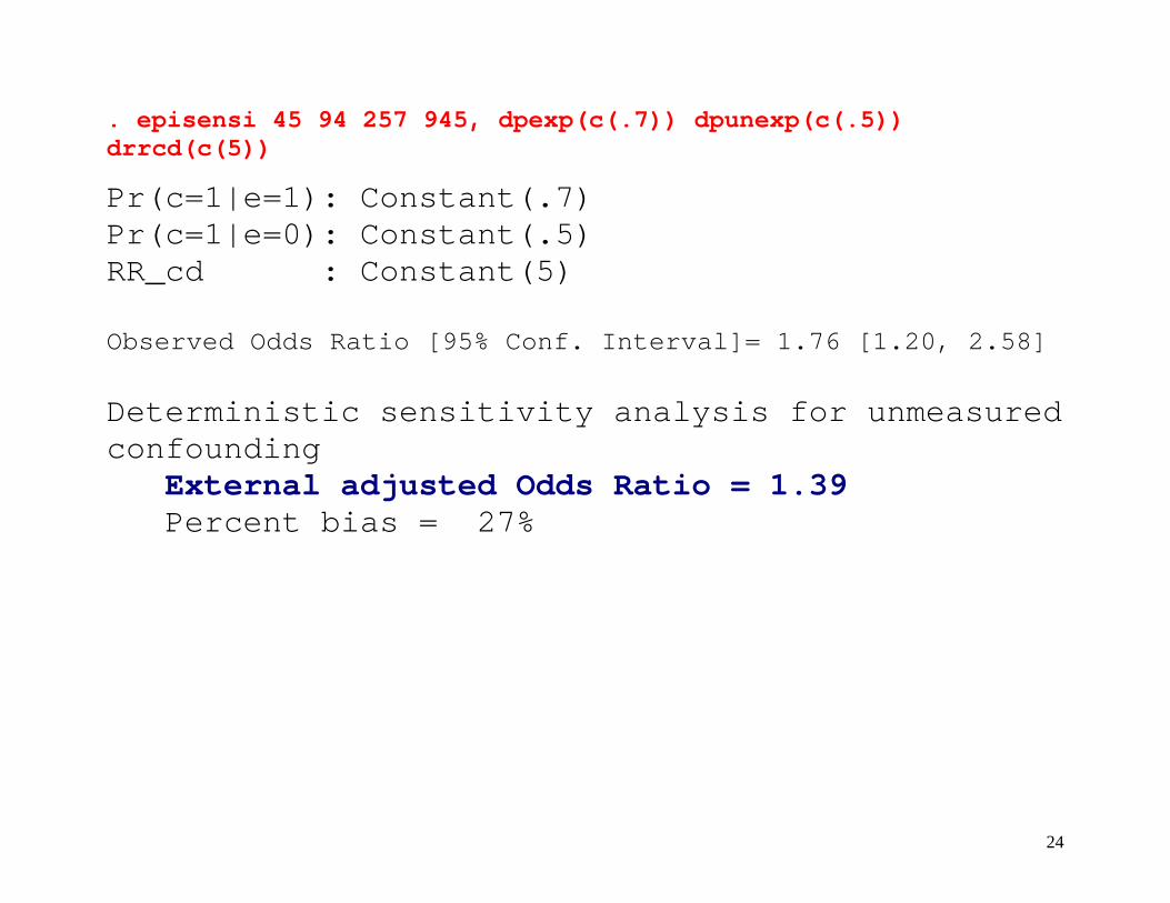
. episensi 45 94 257 945, dpexp(c(.7)) dpunexp(c(.5)) drrcd(c(5))
Pr(c=1|e=1): Constant(.7) Pr(c=1|e=0): Constant(.5) RR_cd : Constant(5) Observed Odds Ratio [95% Conf. Interval]= 1.76 [1.20, 2.58] Deterministic sensitivity analysis for unmeasured confounding External adjusted Odds Ratio = 1.39 Percent bias = 27%
25
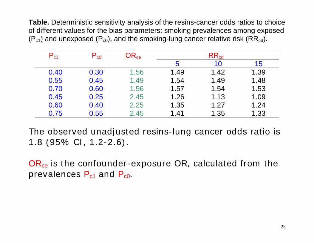
Table. Deterministic sensitivity analysis of the resins-cancer odds ratios to choice of different values for the bias parameters: smoking prevalences among exposed (Pc1) and unexposed (Pc0), and the smoking-lung cancer relative risk (RRcd).
Pc1 Pc0 ORce RRcd 5 10 15
0.40 0.30 1.56 1.49 1.42 1.39 0.55 0.45 1.49 1.54 1.49 1.48 0.70 0.60 1.56 1.57 1.54 1.53 0.45 0.25 2.45 1.26 1.13 1.09 0.60 0.40 2.25 1.35 1.27 1.24 0.75 0.55 2.45 1.41 1.35 1.33
The observed unadjusted resins-lung cancer odds ratio is 1.8 (95% CI, 1.2-2.6). ORce is the confounder-exposure OR, calculated from the prevalences Pc1 and Pc0.
26
Limitation of deterministic sensitivity analysis
• Lack probability structure for the bias parameters
• Fail to discriminate among the different scenarios in
terms of their likelihood
• It is not easy to summarize results
27
Probabilistic sensitivity analysis
A more realistic approach allows for uncertainty in the bias parameters.
By specifying a probability distribution for the bias
parameters, the bias-adjusted relative risk reflects the uncertainty in the bias parameters.
The command episens allows the user to specify a variety of probability densities for the bias parameters, and use these densities to obtain simulation limits for the bias adjusted exposure-disease measure of effect.
28
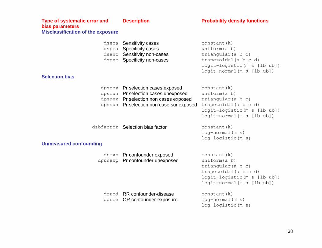
Type of systematic error and bias parameters
Description Probability density functions
Misclassification of the exposure
dseca Sensitivity cases constant(k) dspca Specificity cases uniform(a b) dsenc Sensitivity non-cases triangular(a b c) dspnc Specificity non-cases trapezoidal(a b c d)
logit-logistic(m s [lb ub]) logit-normal(m s [lb ub])
Selection bias
dpscex Pr selection cases exposed constant(k) dpscun Pr selection cases unexposed uniform(a b) dpsnex Pr selection non cases exposed triangular(a b c) dpsnun Pr selection non case sunexposed trapezoidal(a b c d)
logit-logistic(m s [lb ub]) logit-normal(m s [lb ub])
dsbfactor Selection bias factor constant(k) log-normal(m s) log-logistic(m s)
Unmeasured confounding
dpexp Pr confounder exposed constant(k) dpunexp Pr confounder unexposed uniform(a b)
triangular(a b c) trapezoidal(a b c d)
logit-logistic(m s [lb ub]) logit-normal(m s [lb ub])
drrcd RR confounder-disease constant(k) dorce OR confounder-exposure log-normal(m s)
log-logistic(m s)

29
Uniform distribution
01
23
Perc
ent
.5 .6 .7 .8 .9
All the values within the specified bounds (a=.5, b=.9) are equally probable
30
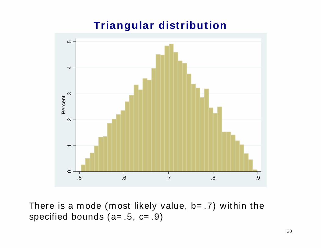
Triangular distribution
01
23
45
Per
cent
.5 .6 .7 .8 .9
There is a mode (most likely value, b=.7) within the specified bounds (a=.5, c=.9)

31
Trapezoidal distribution
01
23
4P
erce
nt
.5 .6 .7 .8 .9
There is an interval of equally probable values between .6 and .8, within specified bounds (.5, .9).
32
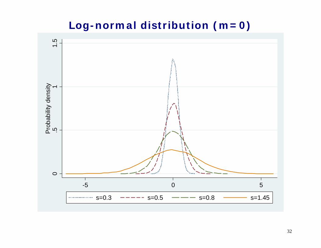
Log-normal distribution (m=0)
0.5
11.
5Pr
obab
ility
dens
ity
-5 0 5
s=0.3 s=0.5 s=0.8 s=1.45
33
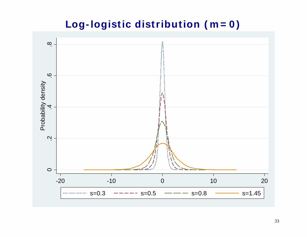
Log-logistic distribution (m=0)
0.2
.4.6
.8P
roba
bilit
y de
nsity
-20 -10 0 10 20
s=0.3 s=0.5 s=0.8 s=1.45
34
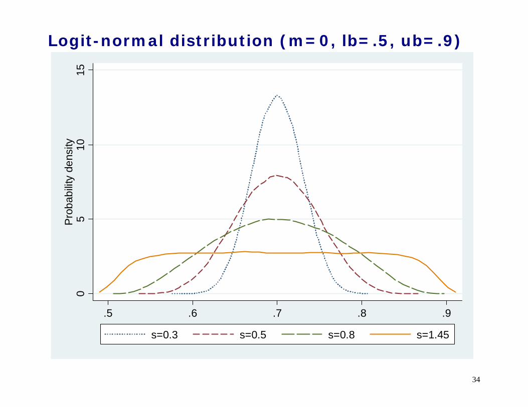
Logit-normal distribution (m=0, lb=.5, ub=.9)
05
1015
Pro
babi
lity
dens
ity
.5 .6 .7 .8 .9
s=0.3 s=0.5 s=0.8 s=1.45
35
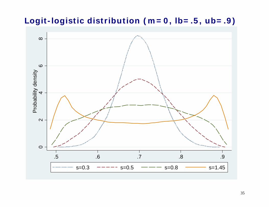
Logit-logistic distribution (m=0, lb=.5, ub=.9)
02
46
8P
roba
bilit
y de
nsity
.5 .6 .7 .8 .9
s=0.3 s=0.5 s=0.8 s=1.45

36
Logit-logistic distribution (m=1, lb=.5, ub=.9)
02
46
810
Prob
abilit
y de
nsity
.5 .6 .7 .8 .9
s=0.3 s=0.5 s=0.8 s=1.45
37
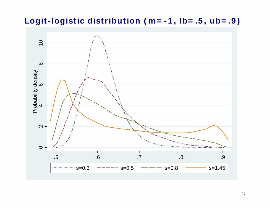
Logit-logistic distribution (m=-1, lb=.5, ub=.9)
02
46
810
Pro
babi
lity
dens
ity
.5 .6 .7 .8 .9
s=0.3 s=0.5 s=0.8 s=1.45
38
Monte Carlo-type simulations
Monte Carlo (random number-based) simulations involve two steps:
step 1) generate a dataset containing observations
from the user specified probability density functions of the bias parameters
step 2) draw a random sample (one set of likely bias
parameters) from this dataset to back-calculate the relative risk
We repeat steps 1 and 2 a large number of times to obtain a distribution of bias-corrected estimates.
39
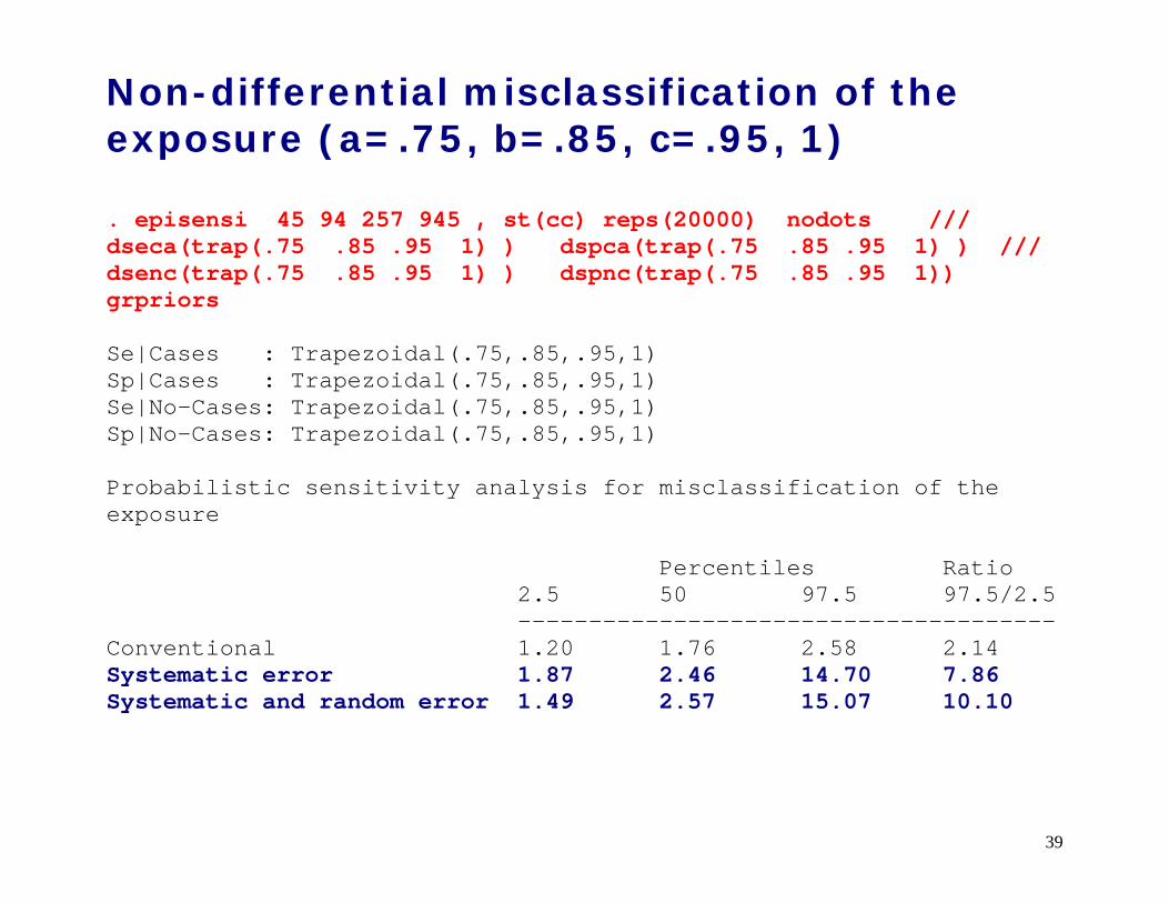
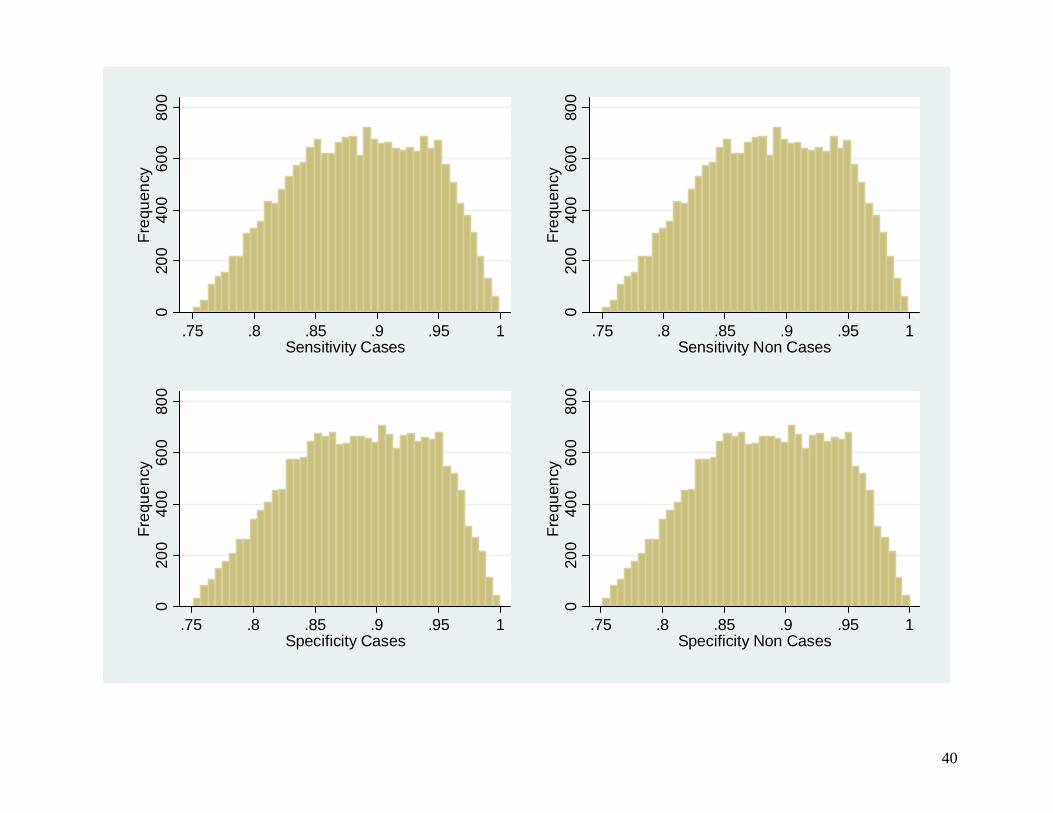
Non-differential misclassification of the exposure (a=.75, b=.85, c=.95, 1) . episensi 45 94 257 945 , st(cc) reps(20000) nodots /// dseca(trap(.75 .85 .95 1) ) dspca(trap(.75 .85 .95 1) ) /// dsenc(trap(.75 .85 .95 1) ) dspnc(trap(.75 .85 .95 1)) grpriors Se|Cases : Trapezoidal(.75,.85,.95,1) Sp|Cases : Trapezoidal(.75,.85,.95,1) Se|No-Cases: Trapezoidal(.75,.85,.95,1) Sp|No-Cases: Trapezoidal(.75,.85,.95,1) Probabilistic sensitivity analysis for misclassification of the exposure Percentiles Ratio 2.5 50 97.5 97.5/2.5 -------------------------------------- Conventional 1.20 1.76 2.58 2.14 Systematic error 1.87 2.46 14.70 7.86 Systematic and random error 1.49 2.57 15.07 10.10
40
020
040
060
080
0Fr
eque
ncy
.75 .8 .85 .9 .95 1Sensitivity Cases
020
040
060
080
0Fr
eque
ncy
.75 .8 .85 .9 .95 1Sensitivity Non Cases
020
040
060
080
0Fr
eque
ncy
.75 .8 .85 .9 .95 1Specificity Cases
020
040
060
080
0Fr
eque
ncy
.75 .8 .85 .9 .95 1Specificity Non Cases
41
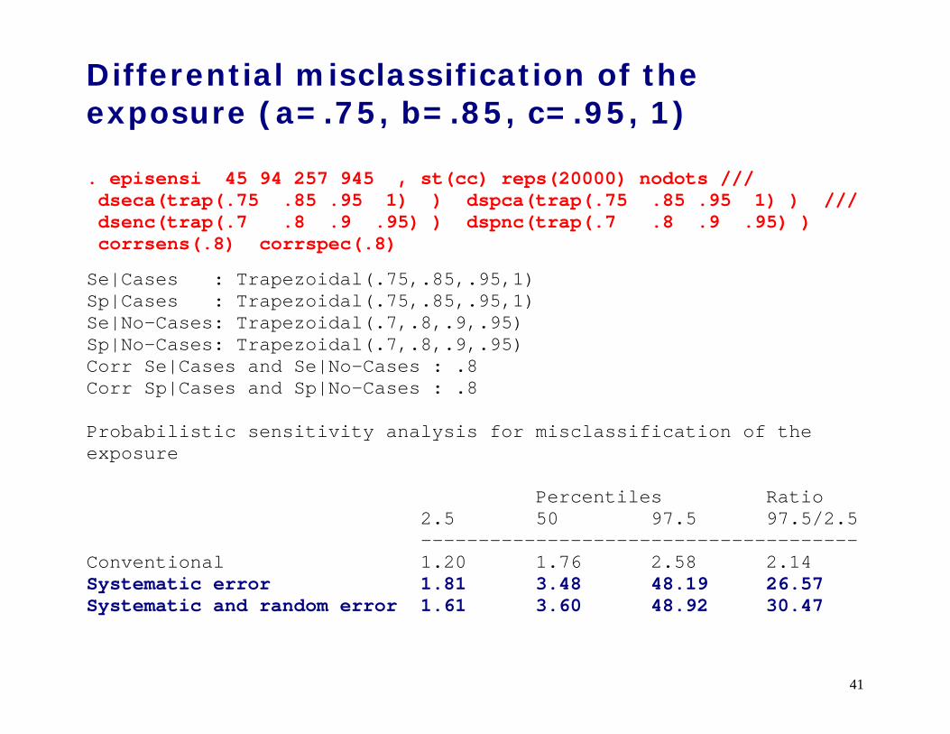
Differential misclassification of the exposure (a=.75, b=.85, c=.95, 1)
. episensi 45 94 257 945 , st(cc) reps(20000) nodots /// dseca(trap(.75 .85 .95 1) ) dspca(trap(.75 .85 .95 1) ) /// dsenc(trap(.7 .8 .9 .95) ) dspnc(trap(.7 .8 .9 .95) ) corrsens(.8) corrspec(.8)
Se|Cases : Trapezoidal(.75,.85,.95,1) Sp|Cases : Trapezoidal(.75,.85,.95,1) Se|No-Cases: Trapezoidal(.7,.8,.9,.95) Sp|No-Cases: Trapezoidal(.7,.8,.9,.95) Corr Se|Cases and Se|No-Cases : .8 Corr Sp|Cases and Sp|No-Cases : .8 Probabilistic sensitivity analysis for misclassification of the exposure Percentiles Ratio 2.5 50 97.5 97.5/2.5 -------------------------------------- Conventional 1.20 1.76 2.58 2.14 Systematic error 1.81 3.48 48.19 26.57 Systematic and random error 1.61 3.60 48.92 30.47
42
Unmeasured confounder
Two uniform distributions for the smoking prevalences among exposed and unexposed between 0.4 and 0.7. The probability density function of the smoking-lung cancer mortality RR is assumed to be log-normal with 95% confidence limits of log(5) and log(15). The limits imply that the mean of this distribution is [(log(15)-log(5)]/2=2.159 with standard deviation [log(15)-log(5)]/2*1.96=0.280.

43
0
100
200
300
400
500
Freq
uenc
y
.4 .5 .6 .7Prevalence confounder exposed
0
100
200
300
400
500
Freq
uenc
y
.4 .5 .6 .7Prevalence confounder unexposed
0
500
1000
1500
2000
Freq
uenc
y
0 10 20 30Confounder-Disease RR

44
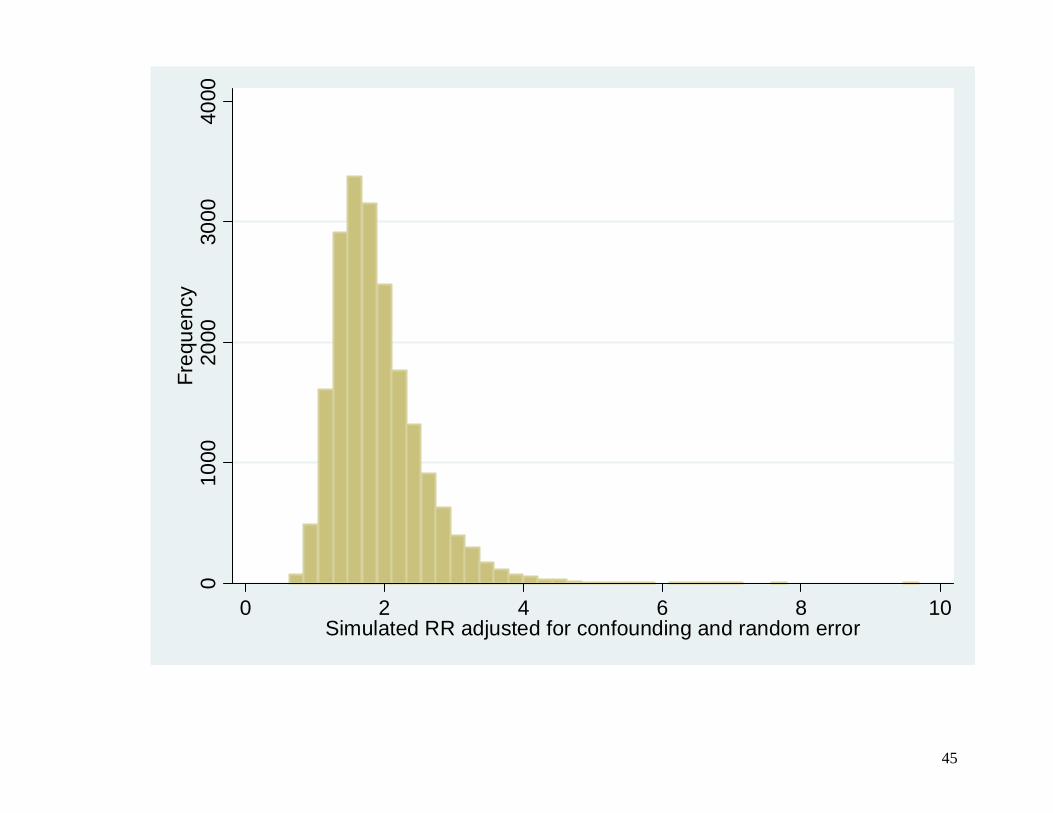
. episensi 45 94 257 945 , st(cc) reps(20000) nodots dpexp(uni(.4 .7)) dpunexp(uni(.4 .7)) drrcd(log-n(2.159 .280)) grarrsys grarrtot grprior Pr(c=1|e=1): Uniform(.4,.7) Pr(c=1|e=0): Uniform(.4,.7) RR_cd : Log-Normal(2.16,0.28) Probabilistic sensitivity analysis for unmeasured confounding Percentiles Ratio 2.5 50 97.5 97.5/2.5 -------------------------------------- Conventional 1.17 1.76 2.61 2.23 Systematic error 1.24 1.76 2.49 2.00 Systematic and random error 1.04 1.76 3.01 2.90
The median smoking-adjusted resins-lung cancer OR is 1.76 with 95% simulation limits of 1.04 and 3.01. As expected, the ratio of the smoking-adjusted simulation limits (2.9) is higher than the ratio of the conventional limits (2.2).
45
010
0020
0030
0040
00Fr
eque
ncy
0 2 4 6 8 10Simulated RR adjusted for confounding and random error

46
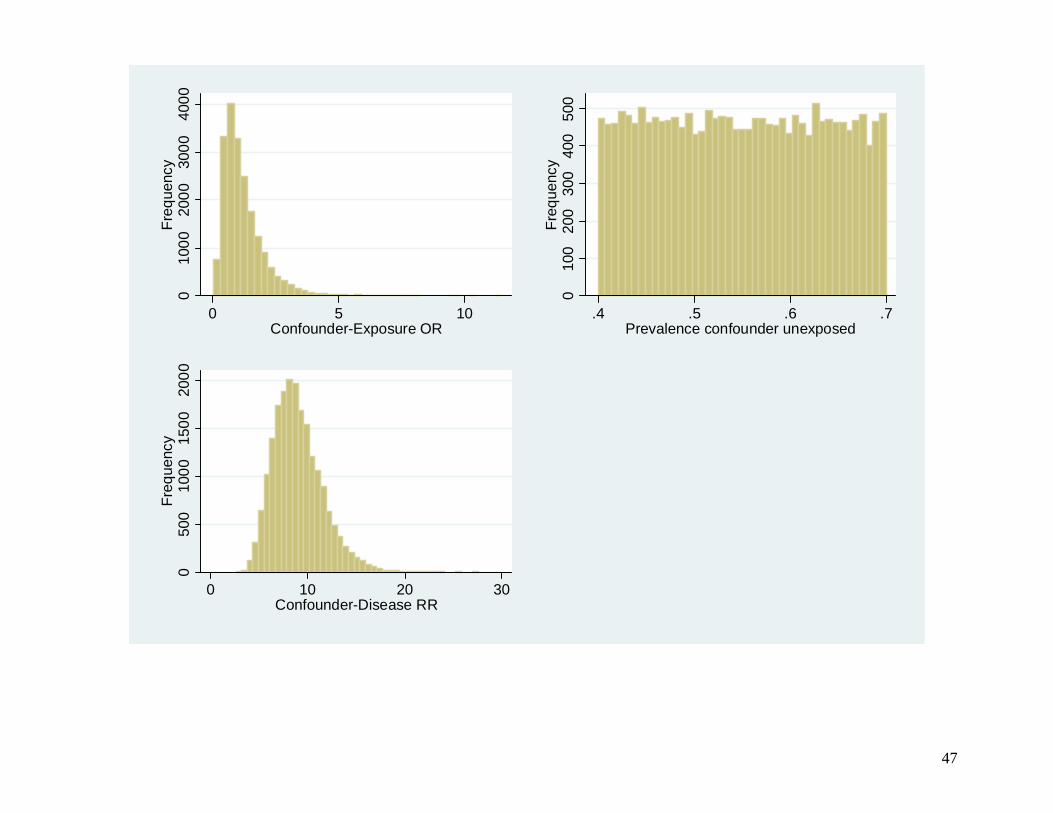
More reasonable priors Given that there is no reason to expect great differences in the prevalence of smoking among resins exposed and unexposed, small differences are more likely than large ones.
One way to address non independent distributions of the confounder-exposure specific prevalences is to specify a probability density function for the confounder-exposure OR (option dorce) instead of the prevalence of the confounder among the exposed (option dpexp).
Assuming independent priors for the confounder-
exposure OR and the prevalence of the confounder among the unexposed is not unreasonable.
47
010
0020
0030
0040
00Fr
eque
ncy
0 5 10Confounder-Exposure OR
010
020
030
040
050
0Fr
eque
ncy
.4 .5 .6 .7Prevalence confounder unexposed
050
010
0015
0020
00Fr
eque
ncy
0 10 20 30Confounder-Disease RR
48
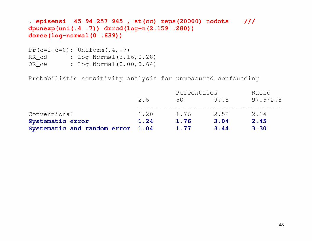
. episensi 45 94 257 945 , st(cc) reps(20000) nodots /// dpunexp(uni(.4 .7)) drrcd(log-n(2.159 .280)) dorce(log-normal(0 .639)) Pr(c=1|e=0): Uniform(.4,.7) RR_cd : Log-Normal(2.16,0.28) OR_ce : Log-Normal(0.00,0.64) Probabilistic sensitivity analysis for unmeasured confounding Percentiles Ratio 2.5 50 97.5 97.5/2.5 -------------------------------------- Conventional 1.20 1.76 2.58 2.14 Systematic error 1.24 1.76 3.04 2.45 Systematic and random error 1.04 1.77 3.44 3.30
49
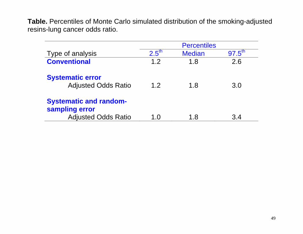
Table. Percentiles of Monte Carlo simulated distribution of the smoking-adjusted resins-lung cancer odds ratio.
Percentiles Type of analysis 2.5th Median 97.5th Conventional 1.2 1.8 2.6 Systematic error Adjusted Odds Ratio 1.2 1.8 3.0 Systematic and random-sampling error
Adjusted Odds Ratio 1.0 1.8 3.4

50
Summary Conventional statistical methods to estimate exposure-disease associations from observational studies are based on several assumptions. When such assumptions are not met, however, the point and interval estimates for the association between exposure and disease are likely to be biased and fail to capture the uncertainty around them. Deterministic (traditional) sensitivity analysis provides a range of bias-adjusted exposure-disease OR, based on observed data and some hypothetical level of bias. In more realistic scenario, probabilistic sensitivity analysis provides a distribution of bias-adjusted exposure-disease OR.
51
Strengths
• Sensitivity analysis helps the investigator to make explicit the location and shape of the distribution of the bias parameters.
• The distributions of the bias parameters reflect the
knowledge and judgment of the investigator about the potential systematic errors that may affect the observed findings.
• Probabilistic sensitivity analysis provides a wider
confidence interval that includes both systematic and random error, which conventional analysis fails to consider (too narrow).
52
Limitations
• Concerns have been raised by some about the arbitrariness in the particular distributions assumed for the bias parameters, which can lead to different distributions of the adjusted exposure-disease RR.
• However, it should be emphasized that in order to
make a shared and meaningful bias correction of the exposure-disease RR, the distributions of the bias parameters should be based on the best available evidence and by careful judgment.
• Informed sensitivity analysis is therefore limited by
lack of data and/or scientific knowledge about the role of bias in a specific exposure-disease association.
53
Download Latest version on my website http://nicolaorsini.altervista.org/
Install the commands, from within Stata, typing at the command line: . net from http://nicolaorsini.altervista.org/stata/ . net install episens

54
Acknowledgments I would like to thank co-authors and project collaborators
• Rino Bellocco
• Matteo Bottai
• Alicja Wolk
• Sander Greenland
55
References
Greenland S, Lash TL. Bias analysis. Ch. 19 in Rothman KJ, Greenland S, Lash TL. Modern Epidemiology, 3rd ed. Philadelphia, PA: Lippincott-Raven, 2008 (in press).
Cornfield J, Haenszel W, Hammond EC, Lilienfeld AM, Shimkin MB, Wynder EL. Smoking and lung cancer:
recent evidence and a discussion of some questions. J Natl Cancer Inst 1959;22:173-203. Friberg E, Mantzoros CS, Wolk A. Physical activity and risk of endometrial cancer: a population-based
prospective cohort study. Cancer Epidemiol Biomarkers Prev 2006;15:2136-40. Greenland S. Basic methods for sensitivity analysis of biases. Int J Epidemiol 1996;25:1107-16. Greenland S. Multiple-bias modelling for analysis of observational data. Journal of the Royal Statistical
Society Series a-Statistics in Society 2005;168:267-291. Jurek AM, Maldonado G, Greenland S, Church TR. Exposure-measurement error is frequently ignored
when interpreting epidemiologic study results. Eur J Epidemiol 2006. Lin DY, Psaty BM, Kronmal RA. Assessing the sensitivity of regression results to unmeasured confounders
in observational studies. Biometrics 1998;54:948-63. Phillips CV. Quantifying and reporting uncertainty from systematic errors. Epidemiology 2003;14:459-66. Rosenbaum PR, Rubin DB. Assessing Sensitivity to an Unobserved Binary Covariate in an Observational
Study with Binary Outcome. Journal of the Royal Statistical Society Series B-Methodological 1983;45:212-218.
Schlesselman JJ. Assessing effects of confounding variables. Am J Epidemiol 1978;108:3-8. Steenland K, Greenland S. Monte Carlo sensitivity analysis and Bayesian analysis of smoking as an
unmeasured confounder in a study of silica and lung cancer. Am J Epidemiol 2004;160:384-92.