probabilistic and bayesian analytics - supsijuergen/mooreprob.pdf · probabilistic analytics: slide...
TRANSCRIPT
Probabilistic andBayesian Analytics
Based on a Tutorial by Andrew W. Moore,Carnegie Mellon University
www.cs.cmu.edu/~awm/tutorials

Probabilistic Analytics: Slide 2
Discrete Random Variables• A is a Boolean-valued random variable if A
denotes an event, and there is somedegree of uncertainty as to whether Aoccurs.
• Examples• A = The US president in 2023 will be male• A = You wake up tomorrow with a headache• A = You have Ebola
Probabilistic Analytics: Slide 3
Probabilities• We write P(A) as “the fraction of possible
worlds in which A is true”• We could at this point spend 2 hours on the
philosophy of this.• But we won’t.
Probabilistic Analytics: Slide 4
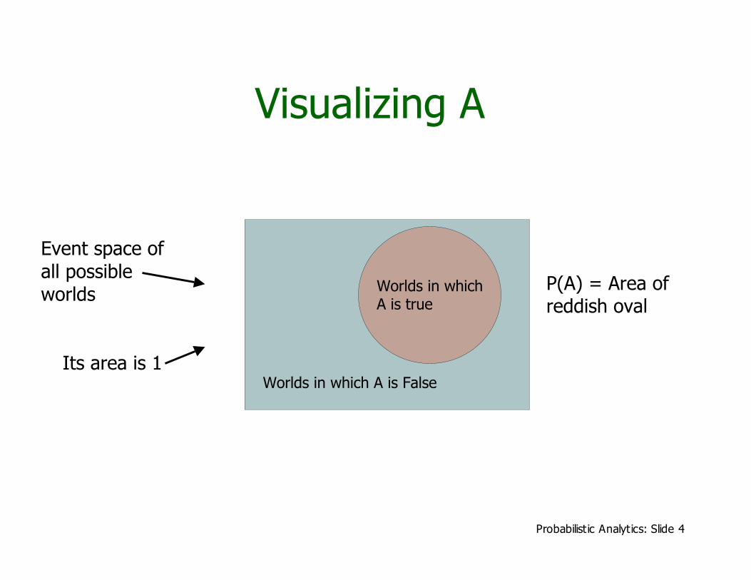
Visualizing A
Event space ofall possibleworlds
Its area is 1Worlds in which A is False
Worlds in whichA is true
P(A) = Area ofreddish oval

Probabilistic Analytics: Slide 5
The Axioms of Probability• 0 <= P(A) <= 1• P(True) = 1• P(False) = 0• P(A or B) = P(A) + P(B) - P(A and B)
Where do these axioms come from? Were they “discovered”?Answers coming up later.

Probabilistic Analytics: Slide 6
Interpreting the axioms• 0 <= P(A) <= 1• P(True) = 1• P(False) = 0• P(A or B) = P(A) + P(B) - P(A and B)
The area of A can’t getany smaller than 0
And a zero area wouldmean no world couldever have A true
Probabilistic Analytics: Slide 7
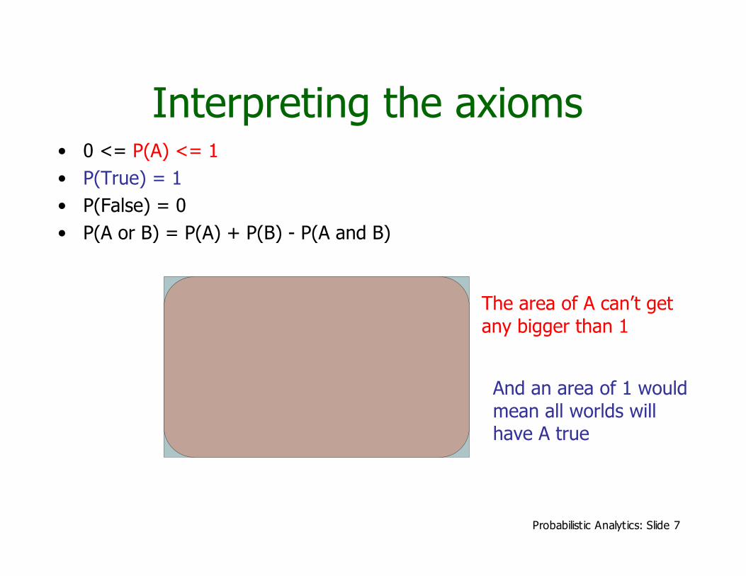
Interpreting the axioms• 0 <= P(A) <= 1• P(True) = 1• P(False) = 0• P(A or B) = P(A) + P(B) - P(A and B)
The area of A can’t getany bigger than 1
And an area of 1 wouldmean all worlds willhave A true

Probabilistic Analytics: Slide 8
Interpreting the axioms• 0 <= P(A) <= 1• P(True) = 1• P(False) = 0• P(A or B) = P(A) + P(B) - P(A and B)
A
B
Probabilistic Analytics: Slide 9
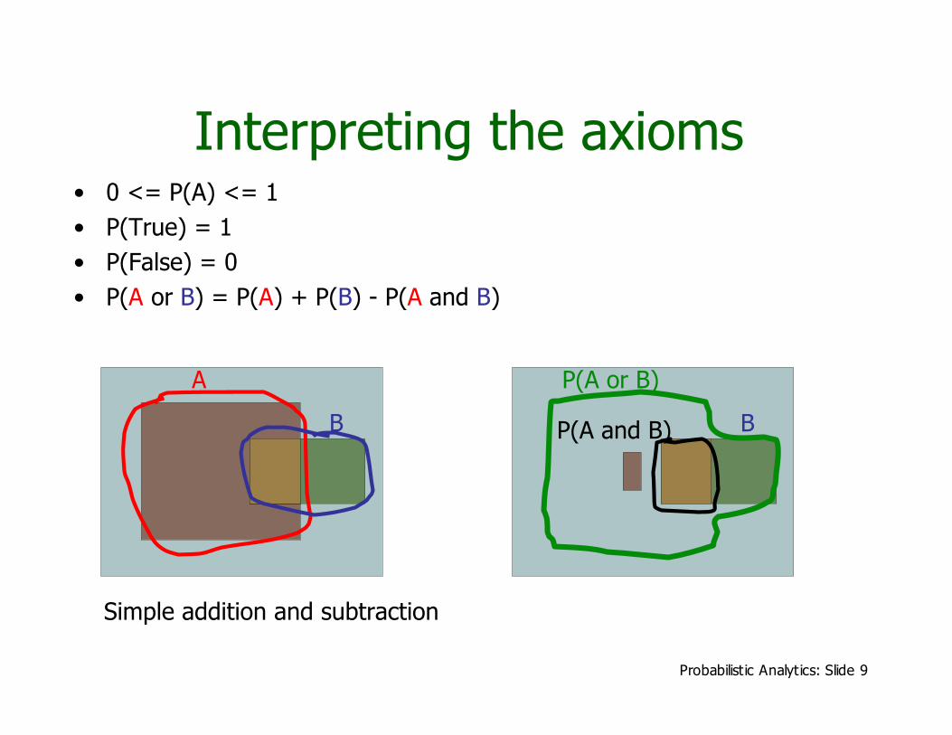
Interpreting the axioms• 0 <= P(A) <= 1• P(True) = 1• P(False) = 0• P(A or B) = P(A) + P(B) - P(A and B)
A
B
P(A or B)
BP(A and B)
Simple addition and subtraction

Probabilistic Analytics: Slide 10
These Axioms are Not to beTrifled With
• There have been attempts to do differentmethodologies for uncertainty
• Fuzzy Logic• Three-valued logic• Dempster-Shafer• Non-monotonic reasoning
• But the axioms of probability are the onlysystem with this property:
If you gamble using them you can’t be unfairly exploitedby an opponent using some other system [di Finetti 1931]

Probabilistic Analytics: Slide 11
Theorems from the Axioms• 0 <= P(A) <= 1, P(True) = 1, P(False) = 0• P(A or B) = P(A) + P(B) - P(A and B)
From these we can prove:P(not A) = P(~A) = 1-P(A)
• How?
Probabilistic Analytics: Slide 12
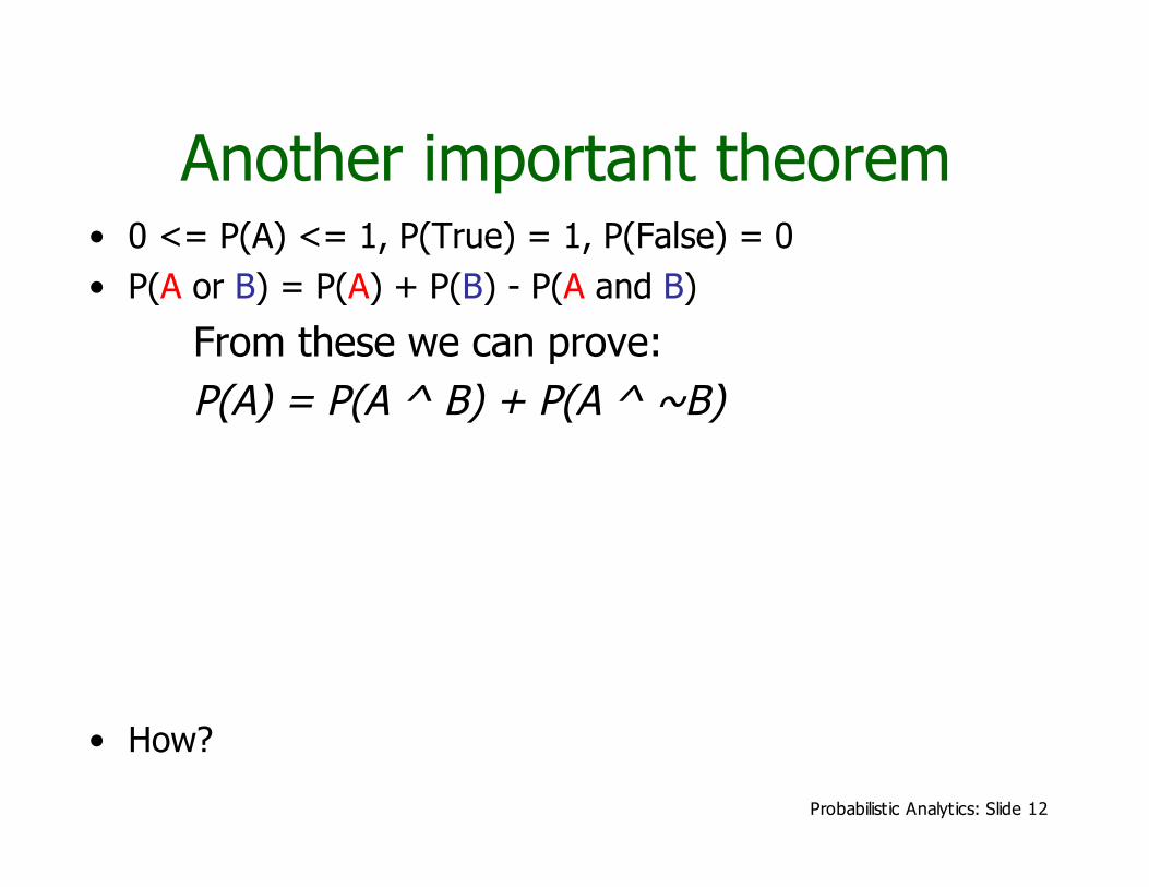
Another important theorem• 0 <= P(A) <= 1, P(True) = 1, P(False) = 0• P(A or B) = P(A) + P(B) - P(A and B)
From these we can prove:P(A) = P(A ^ B) + P(A ^ ~B)
• How?

Probabilistic Analytics: Slide 13
Multivalued Random Variables• Suppose A can take on more than 2 values• A is a random variable with arity k if it can
take on exactly one value out of {v1,v2, ..vk}
• Thus…
jivAvAP ji !=="= if 0)(
1)( 21 ==!=!=kvAvAvAP
Probabilistic Analytics: Slide 14
An easy fact about MultivaluedRandom Variables:
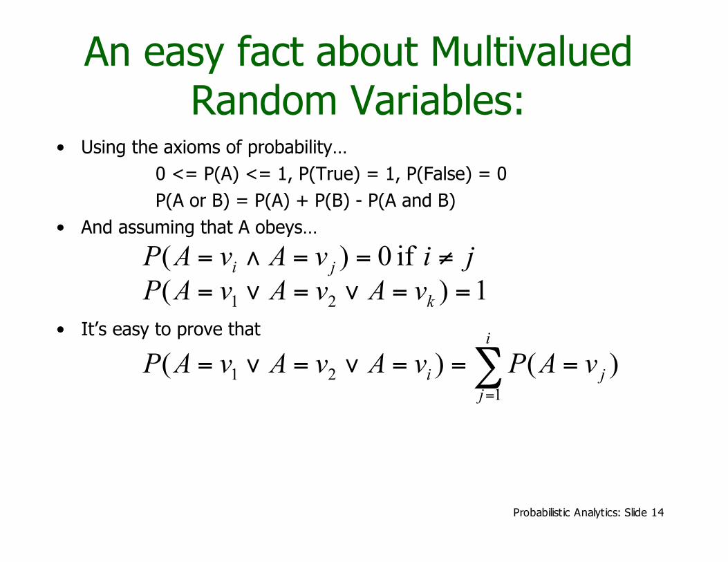
• Using the axioms of probability…0 <= P(A) <= 1, P(True) = 1, P(False) = 0P(A or B) = P(A) + P(B) - P(A and B)
• And assuming that A obeys…
• It’s easy to prove that
jivAvAP ji !=="= if 0)(
1)( 21 ==!=!=kvAvAvAP
)()(1
21 !=
==="="=i
j
ji vAPvAvAvAP

Probabilistic Analytics: Slide 15
An easy fact about MultivaluedRandom Variables:
• Using the axioms of probability…0 <= P(A) <= 1, P(True) = 1, P(False) = 0P(A or B) = P(A) + P(B) - P(A and B)
• And assuming that A obeys…
• It’s easy to prove that
jivAvAP ji !=="= if 0)(
1)( 21 ==!=!=kvAvAvAP
)()(1
21 !=
==="="=i
j
ji vAPvAvAvAP
• And thus we can prove
1)(1
==!=
k
j
jvAP
Probabilistic Analytics: Slide 16
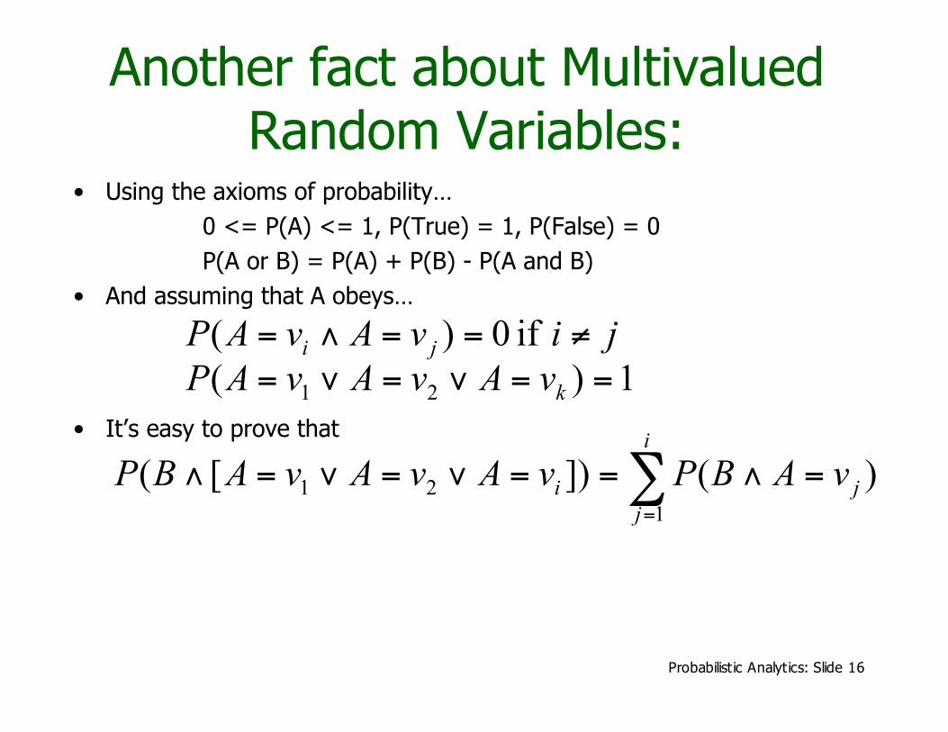
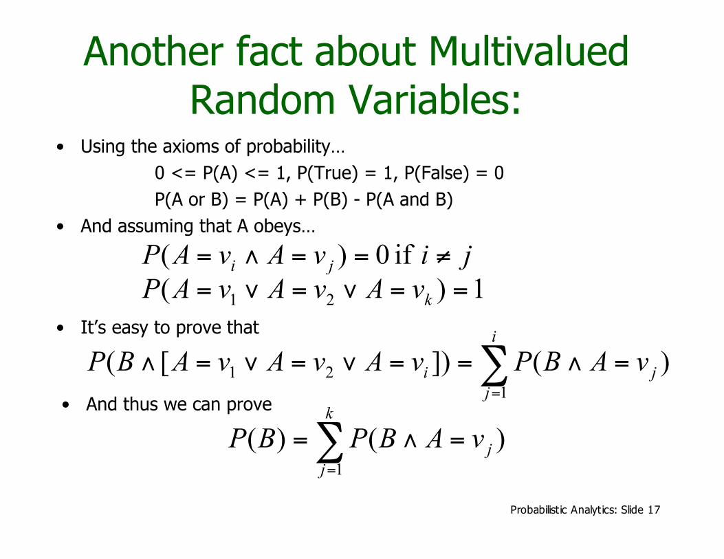
Another fact about MultivaluedRandom Variables:
• Using the axioms of probability…0 <= P(A) <= 1, P(True) = 1, P(False) = 0P(A or B) = P(A) + P(B) - P(A and B)
• And assuming that A obeys…
• It’s easy to prove that
jivAvAP ji !=="= if 0)(
1)( 21 ==!=!=kvAvAvAP
)(])[(1
21 !=
="==#=#="i
j
ji vABPvAvAvABP
Probabilistic Analytics: Slide 17
Another fact about MultivaluedRandom Variables:
• Using the axioms of probability…0 <= P(A) <= 1, P(True) = 1, P(False) = 0P(A or B) = P(A) + P(B) - P(A and B)
• And assuming that A obeys…
• It’s easy to prove that
jivAvAP ji !=="= if 0)(
1)( 21 ==!=!=kvAvAvAP
)(])[(1
21 !=
="==#=#="i
j
ji vABPvAvAvABP
• And thus we can prove
)()(1
!=
="=k
j
jvABPBP

Probabilistic Analytics: Slide 18
Elementary Probability in Pictures• P(~A) + P(A) = 1

Probabilistic Analytics: Slide 19
Elementary Probability in Pictures• P(B) = P(B ^ A) + P(B ^ ~A)

Probabilistic Analytics: Slide 20
Elementary Probability in Pictures1)(
1
==!=
k
j
jvAP

Probabilistic Analytics: Slide 21
Elementary Probability in Pictures)()(
1
!=
="=k
j
jvABPBP
Probabilistic Analytics: Slide 22
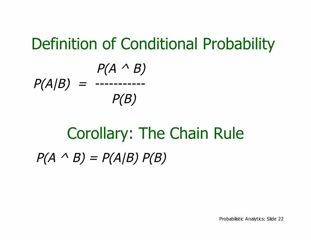
Definition of Conditional Probability P(A ^ B) P(A|B) = ----------- P(B)
Corollary: The Chain RuleP(A ^ B) = P(A|B) P(B)
Probabilistic Analytics: Slide 23
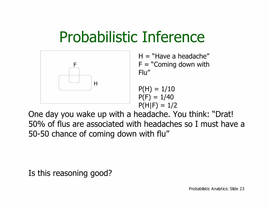
Probabilistic Inference
F
H
H = “Have a headache”F = “Coming down withFlu”
P(H) = 1/10P(F) = 1/40P(H|F) = 1/2
One day you wake up with a headache. You think: “Drat!50% of flus are associated with headaches so I must have a50-50 chance of coming down with flu”
Is this reasoning good?

Probabilistic Analytics: Slide 24
Bayes Rule P(A ^ B) P(A|B) P(B)P(B|A) = ----------- = --------------- P(A) P(A)
This is Bayes Rule
Bayes, Thomas (1763) An essaytowards solving a problem in thedoctrine of chances. PhilosophicalTransactions of the Royal Society ofLondon, 53:370-418

Probabilistic Analytics: Slide 25
More General Forms of Bayes Rule
)(~)|~()()|(
)()|()|(
APABPAPABP
APABPBAP
+=
)(
)()|()|(
XBP
XAPXABPXBAP
!
!!=!

Probabilistic Analytics: Slide 26
More General Forms of Bayes Rule
!=
==
====
An
k
kk
ii
i
vAPvABP
vAPvABPBvAP
1
)()|(
)()|()|(

Probabilistic Analytics: Slide 27
Useful Easy-to-prove facts1)|()|( =¬+ BAPBAP
1)|(1
==!=
An
k
kBvAP

Probabilistic Analytics: Slide 28
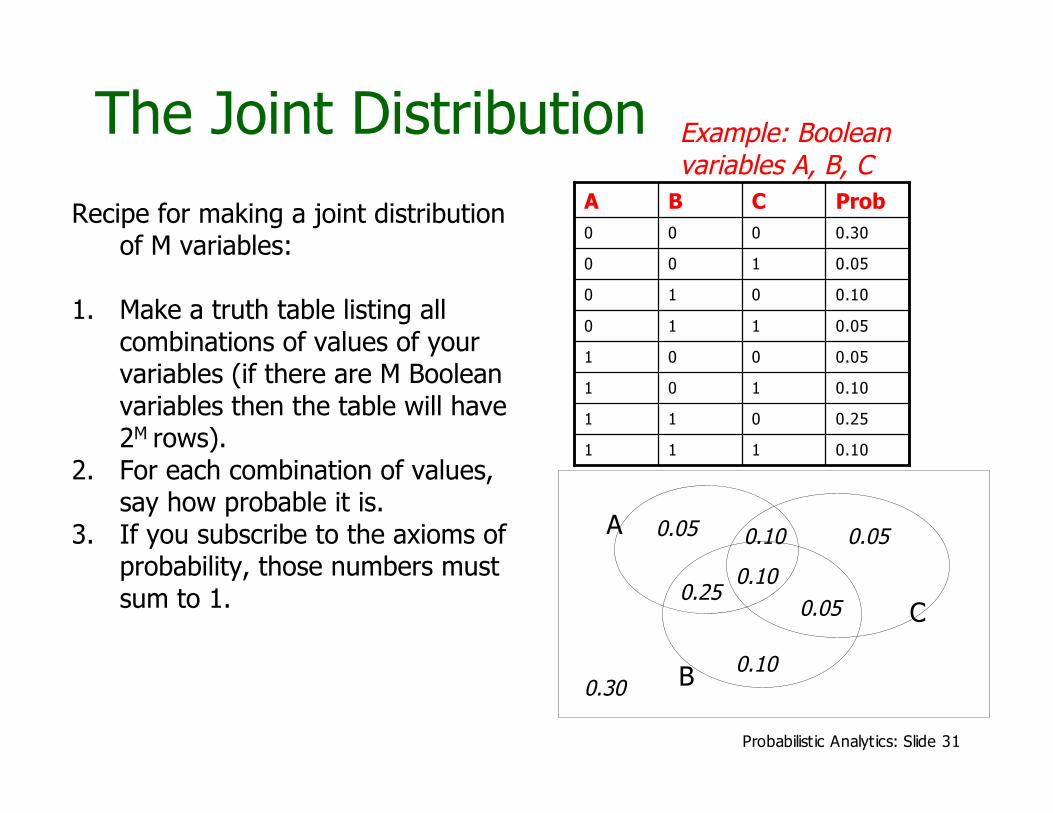
The Joint Distribution
Recipe for making a joint distributionof M variables:
Example: Booleanvariables A, B, C

Probabilistic Analytics: Slide 29
The Joint Distribution
Recipe for making a joint distributionof M variables:
1. Make a truth table listing allcombinations of values of yourvariables (if there are M Booleanvariables then the table will have2M rows).
Example: Booleanvariables A, B, C
111
011
101
001
110
010
100
000
CBA

Probabilistic Analytics: Slide 30
The Joint Distribution
Recipe for making a joint distributionof M variables:
1. Make a truth table listing allcombinations of values of yourvariables (if there are M Booleanvariables then the table will have2M rows).
2. For each combination of values,say how probable it is.
Example: Booleanvariables A, B, C
0.10111
0.25011
0.10101
0.05001
0.05110
0.10010
0.05100
0.30000
ProbCBA
Probabilistic Analytics: Slide 31
The Joint Distribution
Recipe for making a joint distributionof M variables:
1. Make a truth table listing allcombinations of values of yourvariables (if there are M Booleanvariables then the table will have2M rows).
2. For each combination of values,say how probable it is.
3. If you subscribe to the axioms ofprobability, those numbers mustsum to 1.
Example: Booleanvariables A, B, C
0.10111
0.25011
0.10101
0.05001
0.05110
0.10010
0.05100
0.30000
ProbCBA
A
B
C0.050.25
0.10 0.050.05
0.10
0.100.30

Probabilistic Analytics: Slide 32
Using theJoint
One you have the JD youcan ask for the probability ofany logical expressioninvolving your attribute
!=E
PEP
matching rows
)row()(

Probabilistic Analytics: Slide 33
Using theJoint
P(Poor Male) = 0.4654 !=E
PEP
matching rows
)row()(

Probabilistic Analytics: Slide 34
Using theJoint
P(Poor) = 0.7604 !=E
PEP
matching rows
)row()(
Probabilistic Analytics: Slide 35
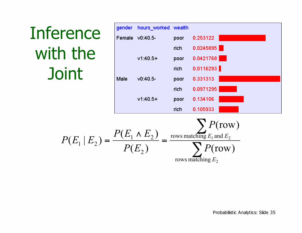
Inferencewith the
Joint
!
!=
"=
2
2 1
matching rows
and matching rows
2
2121
)row(
)row(
)(
)()|(
E
EE
P
P
EP
EEPEEP

Probabilistic Analytics: Slide 36
Inferencewith the
Joint
!
!=
"=
2
2 1
matching rows
and matching rows
2
2121
)row(
)row(
)(
)()|(
E
EE
P
P
EP
EEPEEP
P(Male | Poor) = 0.4654 / 0.7604 = 0.612

Probabilistic Analytics: Slide 37
Inference is a big deal• I’ve got this evidence. What’s the chance
that this conclusion is true?• I’ve got a sore neck: how likely am I to have meningitis?• I see my lights are out and it’s 9pm. What’s the chance
my spouse is already asleep?
Probabilistic Analytics: Slide 38
Inference is a big deal• I’ve got this evidence. What’s the chance
that this conclusion is true?• I’ve got a sore neck: how likely am I to have meningitis?• I see my lights are out and it’s 9pm. What’s the chance
my spouse is already asleep?
Probabilistic Analytics: Slide 39
Inference is a big deal• I’ve got this evidence. What’s the chance
that this conclusion is true?• I’ve got a sore neck: how likely am I to have meningitis?• I see my lights are out and it’s 9pm. What’s the chance
my spouse is already asleep?
• There’s a thriving set of industries growing basedaround Bayesian Inference. Highlights are:Medicine, Pharma, Help Desk Support, EngineFault Diagnosis

Probabilistic Analytics: Slide 40
Where do Joint Distributionscome from?
• Idea One: Expert Humans• Idea Two: Simpler probabilistic facts and
some algebraExample: Suppose you knew
P(A) = 0.7
P(B|A) = 0.2P(B|~A) = 0.1
P(C|A^B) = 0.1P(C|A^~B) = 0.8P(C|~A^B) = 0.3P(C|~A^~B) = 0.1
Then you canautomatically compute theJD using the chain rule
P(A=x ^ B=y ^ C=z) =P(C=z|A=x^ B=y) P(B=y|A=x) P(A=x)
In anotherlecture: BayesNets, asystematic way todo this.

Probabilistic Analytics: Slide 41
Where do Joint Distributionscome from?
• Idea Three: Learn them from data!
Prepare to see one of the most impressive learningalgorithms you’ll come across in the entire course….

Probabilistic Analytics: Slide 42
Learning a joint distributionBuild a JD table for yourattributes in which theprobabilities are unspecified
The fill in each row with
records ofnumber total
row matching records)row(ˆ =P
?111
?011
?101
?001
?110
?010
?100
?000
ProbCBA
0.10111
0.25011
0.10101
0.05001
0.05110
0.10010
0.05100
0.30000
ProbCBA
Fraction of all records in whichA and B are True but C is False

Probabilistic Analytics: Slide 43
Example of Learning a Joint• This Joint
was obtainedby learningfrom threeattributes inthe UCI“Adult”CensusDatabase[Kohavi 1995]

Probabilistic Analytics: Slide 44
Where are we?• We have recalled the fundamentals of
probability• We have become content with what JDs are
and how to use them• And we even know how to learn JDs from
data.
Probabilistic Analytics: Slide 45
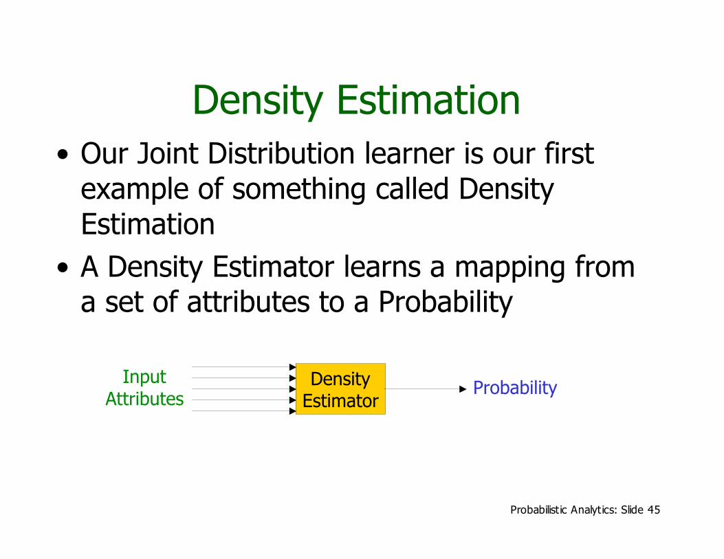
Density Estimation• Our Joint Distribution learner is our first
example of something called DensityEstimation
• A Density Estimator learns a mapping froma set of attributes to a Probability
DensityEstimator
ProbabilityInputAttributes
Probabilistic Analytics: Slide 46
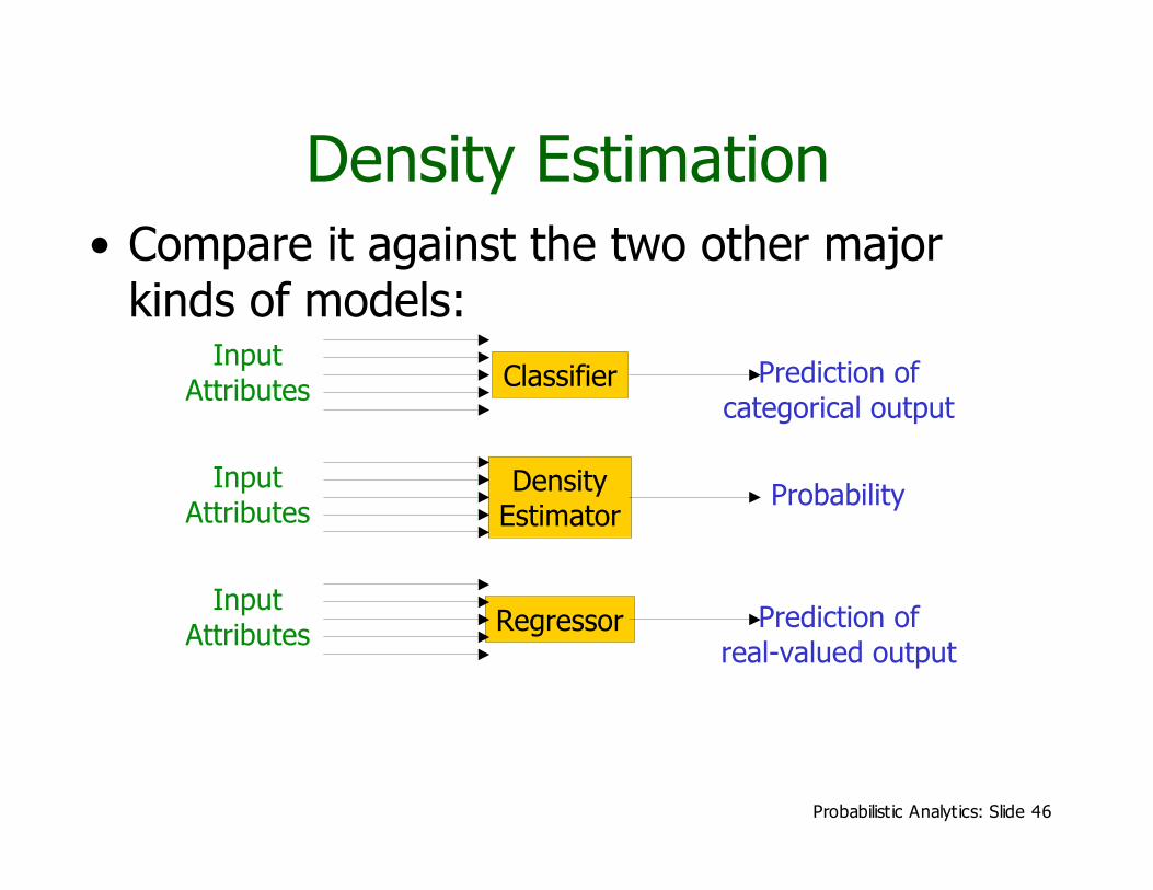
Density Estimation• Compare it against the two other major
kinds of models:
Regressor Prediction ofreal-valued output
InputAttributes
DensityEstimator
ProbabilityInputAttributes
Classifier Prediction ofcategorical output
InputAttributes

Probabilistic Analytics: Slide 47
Evaluating Density Estimation
Regressor Prediction ofreal-valued output
InputAttributes
DensityEstimator
ProbabilityInputAttributes
Classifier Prediction ofcategorical output
InputAttributes
Test setAccuracy
?
Test setAccuracy
Test-set criterion for estimating performanceon future data** See the Decision Tree or Cross Validation lecture for more detail

Probabilistic Analytics: Slide 48
• Given a record x, a density estimator M cantell you how likely the record is:
• Given a dataset with R records, a densityestimator can tell you how likely thedataset is:(Under the assumption that all records were
independently generated from the Density Estimator’sJD)
Evaluating a density estimator
!=
=""=R
k
kR |MP|MP|MP1
21 )(ˆ)(ˆ)dataset(ˆ xxxx K
)(ˆ |MP x

Probabilistic Analytics: Slide 49
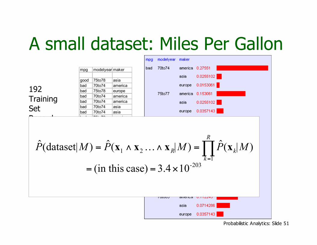
A small dataset: Miles Per Gallon
From the UCI repository (thanks to Ross Quinlan)
192TrainingSetRecords
mpg modelyear maker
good 75to78 asia
bad 70to74 america
bad 75to78 europe
bad 70to74 america
bad 70to74 america
bad 70to74 asia
bad 70to74 asia
bad 75to78 america
: : :
: : :
: : :
bad 70to74 america
good 79to83 america
bad 75to78 america
good 79to83 america
bad 75to78 america
good 79to83 america
good 79to83 america
bad 70to74 america
good 75to78 europe
bad 75to78 europe

Probabilistic Analytics: Slide 50
A small dataset: Miles Per Gallon
192TrainingSetRecords
mpg modelyear maker
good 75to78 asia
bad 70to74 america
bad 75to78 europe
bad 70to74 america
bad 70to74 america
bad 70to74 asia
bad 70to74 asia
bad 75to78 america
: : :
: : :
: : :
bad 70to74 america
good 79to83 america
bad 75to78 america
good 79to83 america
bad 75to78 america
good 79to83 america
good 79to83 america
bad 70to74 america
good 75to78 europe
bad 75to78 europe
Probabilistic Analytics: Slide 51
A small dataset: Miles Per Gallon
192TrainingSetRecords
mpg modelyear maker
good 75to78 asia
bad 70to74 america
bad 75to78 europe
bad 70to74 america
bad 70to74 america
bad 70to74 asia
bad 70to74 asia
bad 75to78 america
: : :
: : :
: : :
bad 70to74 america
good 79to83 america
bad 75to78 america
good 79to83 america
bad 75to78 america
good 79to83 america
good 79to83 america
bad 70to74 america
good 75to78 europe
bad 75to78 europe
203-1
21
10 3.4 case) (in this
)(ˆ)(ˆ)dataset(ˆ
!==
=""= #=
R
k
kR |MP|MP|MP xxxx K

Probabilistic Analytics: Slide 52
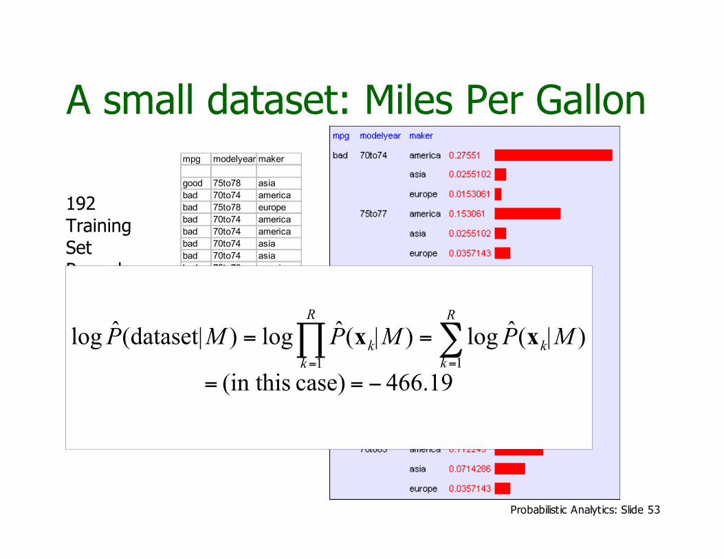
Log Probabilities
Since probabilities of datasets getso small we usually use logprobabilities
!"==
==R
k
k
R
k
k |MP|MP|MP11
)(ˆlog)(ˆlog)dataset(ˆlog xx
Probabilistic Analytics: Slide 53
A small dataset: Miles Per Gallon
192TrainingSetRecords
mpg modelyear maker
good 75to78 asia
bad 70to74 america
bad 75to78 europe
bad 70to74 america
bad 70to74 america
bad 70to74 asia
bad 70to74 asia
bad 75to78 america
: : :
: : :
: : :
bad 70to74 america
good 79to83 america
bad 75to78 america
good 79to83 america
bad 75to78 america
good 79to83 america
good 79to83 america
bad 70to74 america
good 75to78 europe
bad 75to78 europe
466.19 case) (in this
)(ˆlog)(ˆlog)dataset(ˆlog11
!==
== "#==
R
k
k
R
k
k |MP|MP|MP xx

Probabilistic Analytics: Slide 54
Summary: The Good News• We have a way to learn a Density Estimator
from data.• Density estimators can do many good
things…• Can sort the records by probability, and thus
spot weird records (anomaly detection)• Can do inference: P(E1|E2)
Automatic Doctor / Help Desk etc
• Ingredient for Bayes Classifiers (see later)
Probabilistic Analytics: Slide 55
Summary: The Bad News• Density estimation by directly learning the
joint is trivial, mindless and dangerous

Probabilistic Analytics: Slide 56
Using a test set
An independent test set with 196 cars has a worse log likelihood
(actually it’s a billion quintillion quintillion quintillion quintilliontimes less likely)
….Density estimators can overfit. And the full joint densityestimator is the overfittiest of them all!
Probabilistic Analytics: Slide 57
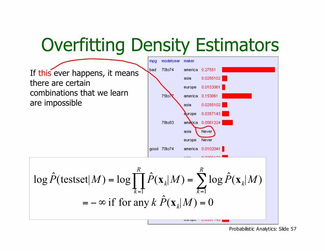
Overfitting Density EstimatorsIf this ever happens, it meansthere are certaincombinations that we learnare impossible
0)(ˆ any for if
)(ˆlog)(ˆlog)testset(ˆlog11
=!"=
== #$==
|MPk
|MP|MP|MP
k
R
k
k
R
k
k
x
xx

Probabilistic Analytics: Slide 58
Using a test set
The only reason that our test set didn’t score -infinity is that mycode is hard-wired to always predict a probability of at least onein 1020
We need Density Estimators that are lessprone to overfitting

Probabilistic Analytics: Slide 59
Naïve Density Estimation
The problem with the Joint Estimator is that it justmirrors the training data.
We need something which generalizes more usefully.
The naïve model generalizes strongly:
Assume that each attribute is distributedindependently of any of the other attributes.
Probabilistic Analytics: Slide 60
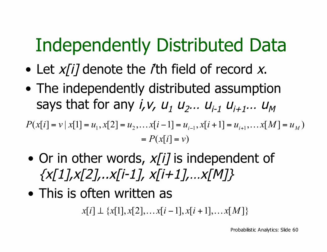
Independently Distributed Data• Let x[i] denote the i’th field of record x.• The independently distributed assumption
says that for any i,v, u1 u2… ui-1 ui+1… uM
)][(
)][,]1[,]1[,]2[,]1[|][( 1121
vixP
uMxuixuixuxuxvixPMii
==
==+=!=== +! KK
• Or in other words, x[i] is independent of{x[1],x[2],..x[i-1], x[i+1],…x[M]}
• This is often written as]}[],1[],1[],2[],1[{][ Mxixixxxix KK +!"

Probabilistic Analytics: Slide 61
A note about independence• Assume A and B are Boolean Random
Variables. Then“A and B are independent”
if and only ifP(A|B) = P(A)
• “A and B are independent” is often notatedas
BA !

Probabilistic Analytics: Slide 62
Independence Theorems• Assume P(A|B) = P(A)• Then P(A^B) =
= P(A) P(B)
• Assume P(A|B) = P(A)• Then P(B|A) =
= P(B)
Probabilistic Analytics: Slide 63
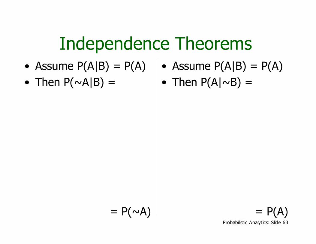
Independence Theorems• Assume P(A|B) = P(A)• Then P(~A|B) =
= P(~A)
• Assume P(A|B) = P(A)• Then P(A|~B) =
= P(A)
Probabilistic Analytics: Slide 64
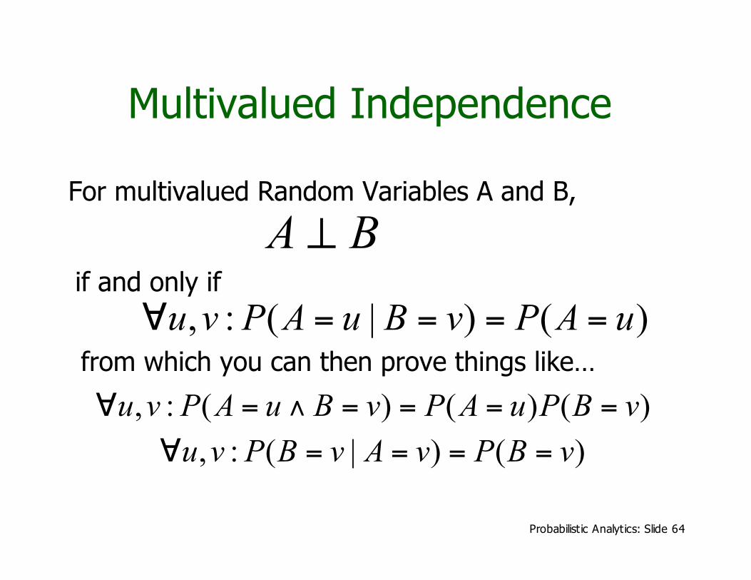
Multivalued Independence
For multivalued Random Variables A and B,
BA !if and only if
)()|(:, uAPvBuAPvu ====!from which you can then prove things like…
)()()(:, vBPuAPvBuAPvu ====!="
)()|(:, vBPvAvBPvu ====!

Probabilistic Analytics: Slide 65
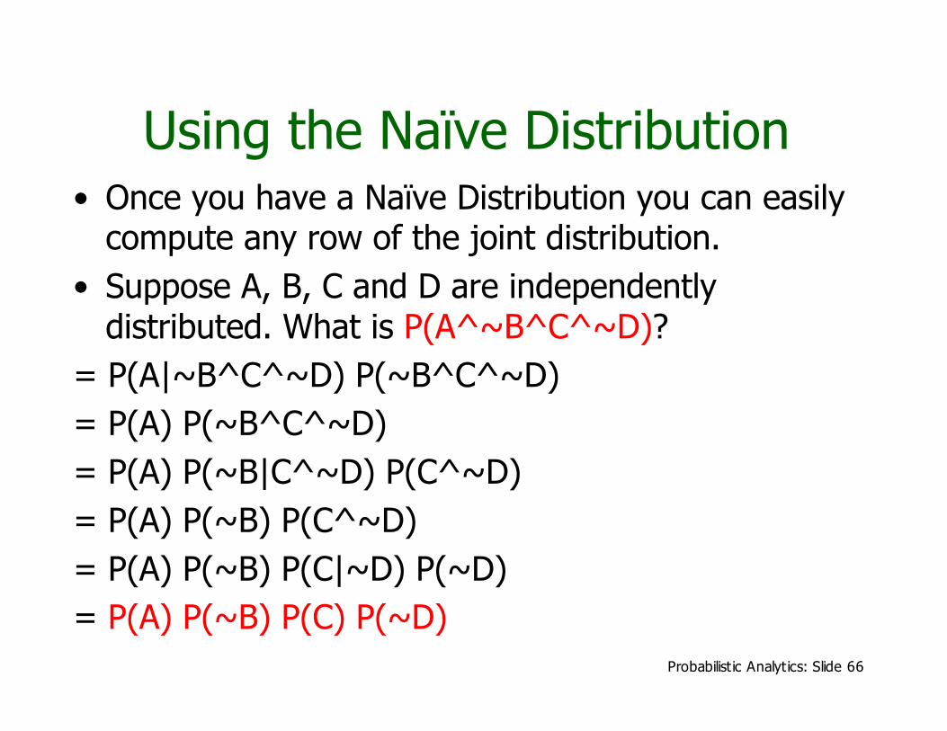
Using the Naïve Distribution• Once you have a Naïve Distribution you can easily
compute any row of the joint distribution.• Suppose A, B, C and D are independently
distributed. What is P(A^~B^C^~D)?
Probabilistic Analytics: Slide 66
Using the Naïve Distribution• Once you have a Naïve Distribution you can easily
compute any row of the joint distribution.• Suppose A, B, C and D are independently
distributed. What is P(A^~B^C^~D)?= P(A|~B^C^~D) P(~B^C^~D)= P(A) P(~B^C^~D)= P(A) P(~B|C^~D) P(C^~D)= P(A) P(~B) P(C^~D)= P(A) P(~B) P(C|~D) P(~D)= P(A) P(~B) P(C) P(~D)

Probabilistic Analytics: Slide 67
Naïve Distribution General Case• Suppose x[1], x[2], … x[M] are independently
distributed.
!=
=====M
k
kMukxPuMxuxuxP
1
21 )][()][,]2[,]1[( K
• So if we have a Naïve Distribution we canconstruct any row of the implied Joint Distributionon demand.
• So we can do any inference• But how do we learn a Naïve Density Estimator?
Probabilistic Analytics: Slide 68
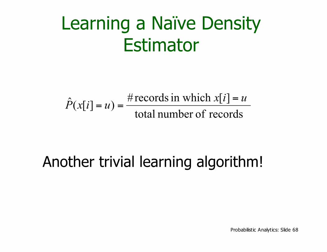
Learning a Naïve DensityEstimator
records ofnumber total
][in which records#)][(ˆ uixuixP
===
Another trivial learning algorithm!

Probabilistic Analytics: Slide 69
Contrast
Given 100 records and 10,000multivalued attributes will be fine
Given 100 records and more than6 Boolean attributes will screw upbadly
Outside Naïve’s scopeNo problem to model “Cis a noisy copy of A”
Can model only veryboring distributions
Can model anything
Naïve DEJoint DE

Probabilistic Analytics: Slide 70
Reminder: The Good News• We have two ways to learn a Density
Estimator from data.• *In other lectures we’ll see vastly more
impressive Density Estimators (Mixture Models,Bayesian Networks, Density Trees, Kernel Densities and many more)
• Density estimators can do many goodthings…• Anomaly detection• Can do inference: P(E1|E2) Automatic Doctor / Help Desk etc
• Ingredient for Bayes Classifiers
Probabilistic Analytics: Slide 71
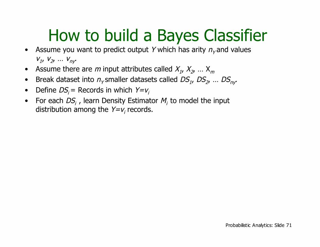
How to build a Bayes Classifier• Assume you want to predict output Y which has arity nY and values
v1, v2, … vny.• Assume there are m input attributes called X1, X2, … Xm
• Break dataset into nY smaller datasets called DS1, DS2, … DSny.• Define DSi = Records in which Y=vi
• For each DSi , learn Density Estimator Mi to model the inputdistribution among the Y=vi records.
Probabilistic Analytics: Slide 72
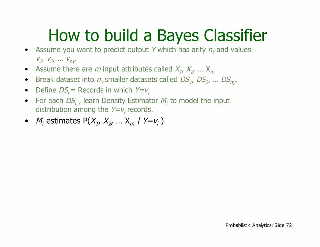
How to build a Bayes Classifier• Assume you want to predict output Y which has arity nY and values
v1, v2, … vny.• Assume there are m input attributes called X1, X2, … Xm
• Break dataset into nY smaller datasets called DS1, DS2, … DSny.• Define DSi = Records in which Y=vi
• For each DSi , learn Density Estimator Mi to model the inputdistribution among the Y=vi records.
• Mi estimates P(X1, X2, … Xm | Y=vi )

Probabilistic Analytics: Slide 73
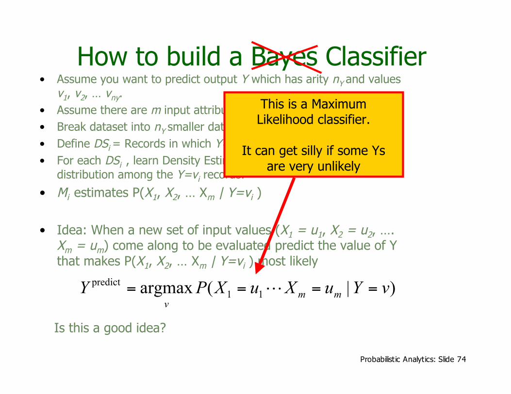
How to build a Bayes Classifier• Assume you want to predict output Y which has arity nY and values
v1, v2, … vny.• Assume there are m input attributes called X1, X2, … Xm
• Break dataset into nY smaller datasets called DS1, DS2, … DSny.• Define DSi = Records in which Y=vi
• For each DSi , learn Density Estimator Mi to model the inputdistribution among the Y=vi records.
• Mi estimates P(X1, X2, … Xm | Y=vi )
• Idea: When a new set of input values (X1 = u1, X2 = u2, ….Xm = um) come along to be evaluated predict the value of Ythat makes P(X1, X2, … Xm | Y=vi ) most likely
)|(argmax 11
predictvYuXuXPY
mm
v
==== L
Is this a good idea?
Probabilistic Analytics: Slide 74
How to build a Bayes Classifier• Assume you want to predict output Y which has arity nY and values
v1, v2, … vny.• Assume there are m input attributes called X1, X2, … Xm
• Break dataset into nY smaller datasets called DS1, DS2, … DSny.• Define DSi = Records in which Y=vi
• For each DSi , learn Density Estimator Mi to model the inputdistribution among the Y=vi records.
• Mi estimates P(X1, X2, … Xm | Y=vi )
• Idea: When a new set of input values (X1 = u1, X2 = u2, ….Xm = um) come along to be evaluated predict the value of Ythat makes P(X1, X2, … Xm | Y=vi ) most likely
)|(argmax 11
predictvYuXuXPY
mm
v
==== L
Is this a good idea?
This is a MaximumLikelihood classifier.
It can get silly if some Ysare very unlikely
Probabilistic Analytics: Slide 75
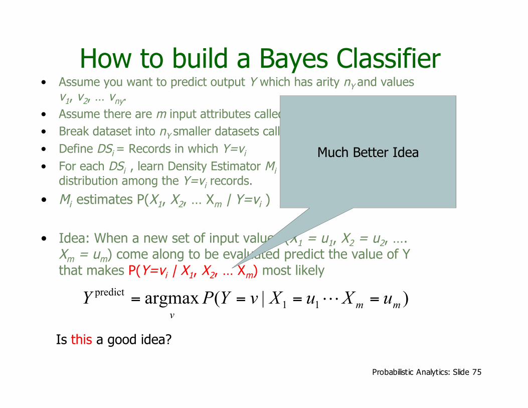
How to build a Bayes Classifier• Assume you want to predict output Y which has arity nY and values
v1, v2, … vny.• Assume there are m input attributes called X1, X2, … Xm
• Break dataset into nY smaller datasets called DS1, DS2, … DSny.• Define DSi = Records in which Y=vi
• For each DSi , learn Density Estimator Mi to model the inputdistribution among the Y=vi records.
• Mi estimates P(X1, X2, … Xm | Y=vi )
• Idea: When a new set of input values (X1 = u1, X2 = u2, ….Xm = um) come along to be evaluated predict the value of Ythat makes P(Y=vi | X1, X2, … Xm) most likely
)|(argmax 11
predict
mm
v
uXuXvYPY ==== L
Is this a good idea?
Much Better Idea
Probabilistic Analytics: Slide 76
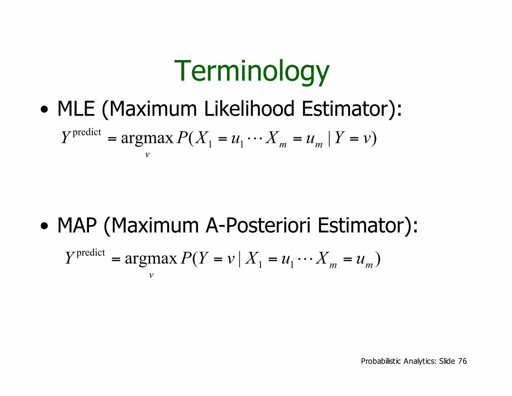
Terminology• MLE (Maximum Likelihood Estimator):
• MAP (Maximum A-Posteriori Estimator):)|(argmax 11
predict
mm
v
uXuXvYPY ==== L
)|(argmax 11
predictvYuXuXPY
mm
v
==== L

Probabilistic Analytics: Slide 77
Getting what we need)|(argmax 11
predict
mm
v
uXuXvYPY ==== L

Probabilistic Analytics: Slide 78
Getting a posterior probability
!=
====
=====
==
=====
===
Yn
j
jjmm
mm
mm
mm
mm
vYPvYuXuXP
vYPvYuXuXP
uXuXP
vYPvYuXuXP
uXuXvYP
1
11
11
11
11
11
)()|(
)()|(
)(
)()|(
)|(
L
L
L
L
L

Probabilistic Analytics: Slide 79
Bayes Classifiers in a nutshell
)()|(argmax
)|(argmax
11
11
predict
vYPvYuXuXP
uXuXvYPY
mm
v
mm
v
=====
====
L
L
1. Learn the distribution over inputs for each value Y.
2. This gives P(X1, X2, … Xm | Y=vi ).
3. Estimate P(Y=vi ). as fraction of records with Y=vi .
4. For a new prediction:

Probabilistic Analytics: Slide 80
Bayes Classifiers in a nutshell
)()|(argmax
)|(argmax
11
11
predict
vYPvYuXuXP
uXuXvYPY
mm
v
mm
v
=====
====
L
L
1. Learn the distribution over inputs for each value Y.
2. This gives P(X1, X2, … Xm | Y=vi ).
3. Estimate P(Y=vi ). as fraction of records with Y=vi .
4. For a new prediction: We can use our favoriteDensity Estimator here.
Right now we have twooptions:
•Joint Density Estimator•Naïve Density Estimator

Probabilistic Analytics: Slide 81
Joint Density Bayes Classifier)()|(argmax 11
predictvYPvYuXuXPY
mm
v
===== L
In the case of the joint Bayes Classifier thisdegenerates to a very simple rule:
Ypredict = the most common value of Y among recordsin which X1 = u1, X2 = u2, …. Xm = um.
Note that if no records have the exact set of inputs X1= u1, X2 = u2, …. Xm = um, then P(X1, X2, … Xm | Y=vi) = 0 for all values of Y.
In that case we just have to guess Y’s value

Probabilistic Analytics: Slide 82
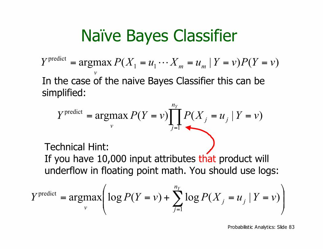
Naïve Bayes Classifier)()|(argmax 11
predictvYPvYuXuXPY
mm
v
===== L
In the case of the naive Bayes Classifier this can besimplified:
!=
====Yn
j
jjv
vYuXPvYPY1
predict )|()(argmax
Probabilistic Analytics: Slide 83
Naïve Bayes Classifier)()|(argmax 11
predictvYPvYuXuXPY
mm
v
===== L
In the case of the naive Bayes Classifier this can besimplified:
!=
====Yn
j
jjv
vYuXPvYPY1
predict )|()(argmax
Technical Hint:If you have 10,000 input attributes that product willunderflow in floating point math. You should use logs:
!!"
#$$%
&==+== '
=
Yn
j
jjv
vYuXPvYPY1
predict )|(log)(logargmax
Probabilistic Analytics: Slide 84
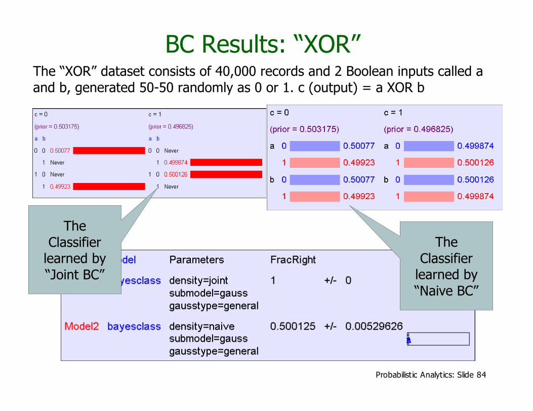
BC Results: “XOR”The “XOR” dataset consists of 40,000 records and 2 Boolean inputs called aand b, generated 50-50 randomly as 0 or 1. c (output) = a XOR b
TheClassifier
learned by“Naive BC”
TheClassifier
learned by“Joint BC”

Probabilistic Analytics: Slide 85
Naïve BC Results: “All Irrelevant”The “all irrelevant” dataset consistsof 40,000 records and 15 Booleanattributes called a,b,c,d..o wherea,b,c are generated 50-50randomly as 0 or 1. v (output) = 1with probability 0.75, 0 with prob0.25
TheClassifier
learned by“Naive BC”

Probabilistic Analytics: Slide 86
More Facts About BayesClassifiers
• Many other density estimators can be slotted in*.• Density estimation can be performed with real-valued
inputs*• Bayes Classifiers can be built with real-valued inputs*• Rather Technical Complaint: Bayes Classifiers don’t try to
be maximally discriminative---they merely try to honestlymodel what’s going on*
• Zero probabilities are painful for Joint and Naïve. A hack(justifiable with the magic words “Dirichlet Prior”) canhelp*.
• Naïve Bayes is wonderfully cheap. And survives 10,000attributes cheerfully!
*See future Andrew Lectures

Probabilistic Analytics: Slide 87
What you should know• Probability
• Fundamentals of Probability and Bayes Rule• What’s a Joint Distribution• How to do inference (i.e. P(E1|E2)) once you
have a JD
• Density Estimation• What is DE and what is it good for• How to learn a Joint DE• How to learn a naïve DE
Probabilistic Analytics: Slide 88
What you should know• Bayes Classifiers
• How to build one• How to predict with a BC• Contrast between naïve and joint BCs