proaches to sequence evolution., springer. 8 molecular...
TRANSCRIPT
Xia, X. 2006. Molecular phylogenetics: mathematical framework and unsolved problems. Pp. 171-191 in U. Bastolla, M. Porto, H. E. Roman, and M. Vendruscolo, eds. Structural ap-proaches to sequence evolution., Springer.
8 Molecular Phylogenetics: Mathematical Framework and Unsolved Problems Xuhua Xia
University of Ottawa, 150 Louis Pasteur, Ottawa, Ontario, Canada K1N 6N5 [email protected]
Abstract. Phylogenetic relationship is essential in dating evolutionary events, reconstructing ancestral genes, predicting sites that are important to natural selection and, ultimately, understanding genomic evolution Three categories of phylogenetic methods are currently used: the distance-based, the maximum parsimony, and the maximum likelihood method. Here I present the mathe-matical framework of these methods and their rationales, provide computa-tional details for each of them, illustrate analytically and numerically the po-tential biases inherent in these methods, and outline computational challenges and unresolved problems. This is followed by a brief discussion of the Bayes-ian approach that has recently been used in molecular phylogenetics.
8.1 Introduction
Biodiversity comes in many colors and shades, and unorganized biodiversity can not only dazzle our eyes but also confuse our minds. Phylogenetics is a special branch of science with the aim to organize biodiversity based on the ancestor-descendent rela-tionship. Molecular phylogenetics uses molecular sequence data to achieve its three main objectives: (1) to reconstruct the branching pattern of different evolutionary lineages such as species and genes, (2) to date evolutionary events such as speciation or gene duplication and subsequent functional divergence, and (3) to understand and summarize the evolutionary processes by substitution models. With the rapid increase of DNA and protein sequence data, and with the realization that DNA is the most reliable indicator of ancestor-descendent relationships, molecular phylogenetics has become one of the most dynamic fields in biology with solid theoretical foundations [1-3] and powerful software tools [4-8]. I will not argue for the importance of mo-lecular phylogenetics other than quoting Aristotle’s statement that “He who sees things from the very beginning has the most advantageous view of them.”
It is not always easy to see things from the very beginning. The evolutionary proc-ess depicted in Fig. 1 shows an ancestral population with a single sequence shared among all individuals that have subsequently split into two populations and evolved and accumulated substitutions independently. Twelve substitutions have occurred, but only three differences can be observed between the sequences from the two extant species. The most fundamental difficulty in molecular phylogenetics is to estimate the true number of substitutions (i.e., 12) from the observed number of differences be-
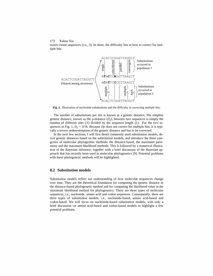
172 Xuhua Xia tween extant sequences (i.e., 3). In short, the difficulty lies in how to correct for mul-tiple hits.
ACACTCGGATTAGGCT
G C
sing
le
para
llel
conv
erge
nt
C
coin
cide
ntal
mul
tiple
back
ACACTCGGATTAGGCT(Shared among ancestors)
ATACTCAGGTTAAGCT
ACATTCCGGTTAAGCT
ACACTCGGATTAGGCT
Substitutions occurred in population 1
Substitutions occurred in population 2m
ultip
le
Fig. 1. Illustration of nucleotide substitutions and the difficulty in correcting multiple hits.
The number of substitutions per site is known as a genetic distance. The simplest genetic distance, known as the p-distance (Dp), between two sequences is simply the number of different sites (N) divided by the sequence length (L). For the two se-quences in Fig. 1, Dp = 3/16. Because Dp does not correct for multiple hits, it is typi-cally a severe underestimation of the genetic distance and has to be corrected.
In the next few sections, I will first detail commonly used substitution models, de-rive genetic distances based on the substitution models, and introduce the three cate-gories of molecular phylogenetic methods: the distance-based, the maximum parsi-mony and the maximum likelihood methods. This is followed by a numerical illustra-tion of the Bayesian inference, together with a brief discussion of the Bayesian ap-proach that has recently been used in molecular phylogenetics [9]. Potential problems with these phylogenetic methods will be highlighted.
8.2 Substitution models
Substitution models reflect our understanding of how molecular sequences change over time. They are the theoretical foundation for computing the genetic distance in the distance-based phylogenetic method and for computing the likelihood value in the maximum likelihood method for phylogenetics. There are three types of molecular sequences, i.e., nucleotide, amino acid and codon sequences. Consequently, there are three types of substitution models, i.e., nucleotide-based, amino acid-based and codon-based. We will focus on nucleotide-based substitution models, with only a brief discussion on amino acid-based and codon-based models to highlight a few potential problems.

8 Molecular Phylogenetics 173 8.2.1 Nucleotide-based substitution models and genetic distances
Let pt be the vector of the four nucleotide frequencies in the order of A, G, C, T at time t. Nucleotide-based substitution models are characterized by a Markov chain of four discrete states as follows:
1
AA AG AC AT
GA GG GC GTt t t
CA CG CC CT
TA TG TC TT
P P P P
P P P Pp p p M
P P P P
P P P P
+ = =
⎡ ⎤⎢ ⎥⎢ ⎥⎢ ⎥⎢ ⎥⎣ ⎦
(8.1)
where M is the transition probability matrix and Pij is the probability of changing from state i to state j in one unit of time. Three frequently used special cases of equa-tion (8.1) will be detailed here: the JC69 model [10], the K80 model [11], and the TN93 model [12].
The simplest nucleotide substitution model is the JC69 one-parameter model, in which all off-diagonal elements in M are identical and designated as α. The four diagonal elements in M are 1-3α constrained by the row sum equal to 1. There is a corresponding rate matrix, designated by Q , that differs from M only in that the di-agonal elements are -3α, constrained by the row sum equal to 0. It is often more con-venient to derive substitution rates by using Q instead of M, as will be clear latter. Following equation (8.1), we have
. 1 . . . .
. 1 . . . .
. 1 . . . .
. 1 . . . .
(1 3 )
(1 3 )
(1 3 )
(1 3 ) .
A t A t G t C t T t
G t A t G t C t T t
C t A t G t C t T t
T t A t G t C t T t
P P P P P
P P P P P
P P P P P
P P P P P
α α α α
α α α α
α α α α
α αα α
+
+
+
+
= − + + +
+ − + +
= + + − +
= + + + −
= (8.2)
Arranging the left side to be PA.t+1 - PA.t and then applying the continuous approxi-
mation, we have
. . . .
. . . .
. . . .
. . . .
(3 ) ( )
(3 ) ( )
(3 ) ( )
(3 ) ( ) .
AA t G t C t T t
GG t A t C t T t
CC t A t G t T t
TT t A t G t C t
PP P P P
tP
P P P Pt
PP P P P
tP
P P P Pt
α α
α α
α α
α α
∂= − + + +
∂∂
= − + + +∂∂
= − + + +∂∂
= − + + +∂
(8.3)
Equation (8.3) is a special case of a general equation. Designate d as the vector of
the four partial derivatives, the general equation is
174 Xuhua Xia td PQ= (8.4)
where Q is the rate matrix mentioned before.
Suppose that we start with nucleotide A, what is the probability that it will stay as A or change to one of the other three nucleotides after time t? Given the initial condi-tion that PA.0 = 1 and PC.0 = PG.0 = PT.0 = 0 and the constrain that that PA + PG + PC + PT = 1, equation (8.3) can be solved to yield
4.
4. . .
1 34 4
1 1.
4 4
tA t
tG t C t T t
P e
P P P e
α
α
−
−
= +
= = = −
(8.5)
The time t in equation (8.5) is the time from the ancestor to the present. When we
compare two extant sequences, the time is 2t, i.e., from one sequence to the ancestor and then back to the other sequence. So equation (8.5) has its general form as
8.
8.
1 34 41 1
.4 4
tii t
tij t
P e
P e
α
α
−
−
= +
= −
(8.6)
The genetic distance (D), which is the number of substitutions per site, is defined
as 2tμ where μ is the rate of substitution. For the JC69 mode, μ = 3α, so αt = D/6. Now we can readily derive D, now designated DJC69, from the probability of a site being different which is estimated by the p-distance (Dp) defined before. According to equation (8.6),
694 / 38.
69
3 31 (1 ) (1 )
4 443
ln(1 ) .4 3
JCDtp ii t
pJC
D P e e
DD
α −−= − = − = −
= − −
(8.7)
For the two sequences in Fig. 1, Dp = 3/16 = 0.1875 and DJC69 = 0.21576. The
equilibrium frequencies are derived by setting (pi.t+1 – pi.t) in equation (8.3) to zero. Solving the resulting simultaneous equations with the constraint that the four fre-quencies sum up to 1, we have PA.t =PG.t =PC.t =PT.t = 0.25. In summary, the JC69 model assumes that (1) the four nucleotides can change into each other with equal probability and (2) the equilibrium frequencies are all equal to 0.25.
The variance of DJC69 can be obtained by using the “delta” method [13]. When a variable Y is a function of a variable X, i.e., Y = F(X), the delta method allows us to obtain approximate formulation of the variance of Y if (1) Y is differentiable with respect to X and (2) the variance of X is known. The same can be extended to more variables.
8 Molecular Phylogenetics 175 The mathematical concept for the delta method is illustrated below, starting with
the simplest case of Y = F(X). Regardless of the functional relationship between Y and X, we always have
dY
Y XdX
Δ ≈ Δ⎛ ⎞⎜ ⎟⎝ ⎠
(8.8)
( ) ( )2
2 2 .dY
Y XdX
Δ ≈ Δ⎛ ⎞⎜ ⎟⎝ ⎠
(8.9)
where ΔY and ΔX are small changes in Y and X, respectively. Note that the variance of Y is the expectation of the squared deviations of Y, i.e.,
2
2
( ) ( )
( ) ( ) .
V Y E Y
V X E X
= Δ
= Δ (8.10)
Replacing (ΔY)2 and (ΔX)2 in equation (8.9) with V(Y) and V(X), we have
2
( ) ( ) .dY
V Y V XdX
≈ ⎛ ⎞⎜ ⎟⎝ ⎠
(8.11)
This relationship allows us to obtain an approximate formulation of the variance of either Y or X if we know either V(X) or V(Y). For the variance of DJC69, we note that DJC69 is a function of Dp, and the variance of Dp is known from the binomial distribu-tion:
(1 )
( ) p pp
D DV D
L
−= (8.12)
where L is the length of the two aligned sequences. From the expression of DJC69 in equation (8.7), we have
69
2
6969 2
14
13
(1 )( ) ( ) .
41
3
JC
p
p pJCJC p
p
p
p
DDD
D DDV D V D
D DL
∂=
∂−
−∂= =
∂−
⎛ ⎞⎜ ⎟⎜ ⎟ ⎛ ⎞⎝ ⎠
⎜ ⎟⎝ ⎠
(8.13)
Kimura [11] noted that transitional substitutions typically occur much more fre-
quently than transversions, and consequently proposed the two-parameter K80 model in which the rate of transitional substitutions (A↔G and T↔C) is designated as α and the rate of transversion substitutions (A↔T, A↔C, G↔T and G↔C) as β. Sub-stituting this new Q into equation (8.4) and solve the equations with the initial condi-tion that PA.0 = 1 and PC.0 = PG.0 = PT.0 = 0 and the constrain that that PA + PG + PC + PT = 1as before, we have
176 Xuhua Xia
4 2( ).
4 2( ).
4. .
1 1 14 4 21 1 14 4 2
1 1 .
4 4
t tA t
t tG t
tC t T t
P e e
P e e
P P e
β α β
β α β
β
− − +
− − +
−
= + +
= + −
= = −
(8.14)
Note again that time t in equation (8.14) should be 2t when used between two ex-
tant sequences. So equation (8.14) has its general form as
8 4( ).
8.
1 1 14 4 21 12 2
t ts t
tv t
P e e
P e
β α β
β
− − +
−
= + −
= −
(8.15)
where Ps.t and Pv.t are the probabilities that a site differs by a transition and a transver-sion, respectively, between two sequences that have diverged for time t, and can be estimated by the proportion of sites differ by a transition (P) and a transversion (Q), respectively. This leads to
ln(1 2 )8
ln(1 2 ) ln(1 2 ).
4 8
Qt
P Q Qt
β
α
−= −
− − −= − +
(8.16)
Recall that the genetic distance is defined as 2tμ where μ = α + 2β for the K80
model. Therefore,
80
1 12 4 ln( ) ln( ), where
2 41 1
and .1- 2 - 1- 2
KD t t a b
a bP Q Q
α β= + = +
= = (8.17)
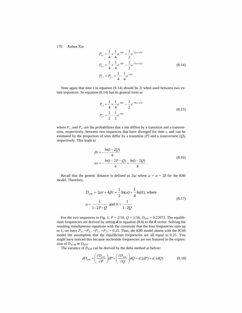
For the two sequences in Fig. 1, P = 2/16, Q = 1/16, DK80 = 0.22073. The equilib-
rium frequencies are derived by setting d in equation (8.4) to the 0 vector. Solving the resulting simultaneous equations with the constraint that the four frequencies sum up to 1, we have PA.t =PG.t =PC.t =PT.t = 0.25. Thus, the K80 model shares with the JC69 model the assumption that the equilibrium frequencies are all equal to 0.25. You might have noticed this because nucleotide frequencies are not featured in the expres-sion of DJC69 or DK80.
The variance of DK80 can be derived by the delta method as before:
80 8080 1 2( ) ( )K K
K
D DdD dP dQ d dP d dQ
P Q∂ ∂
= + = +∂ ∂
⎛ ⎞⎛ ⎞⎜ ⎟ ⎜ ⎟⎝ ⎠ ⎝ ⎠
(8.18)

8 Molecular Phylogenetics 177
[ ]
[ ]
2280 1 2
2 2 2 21 1 2 2
2 21 1 2 2
11 2
2
( ) ( ) ( )
( ) 2 ( ) ( )
( ) 2 ( , ) ( )
( ) ( , ) .
( , ) ( )
KdD d dP d dQ
d dP d d dPdQ d dQ
d V P d d Cov P Q d V Q
dV P Cov P Qd d
dCov P Q V Q
= +
= + +
= + +
=⎡ ⎤⎡ ⎤⎢ ⎥⎢ ⎥
⎣ ⎦ ⎣ ⎦
(8.19)
Recall that P and Q stand for the proportion of sites that differ by a transitional change and differ by a transversional change, respectively. Designate R as the propor-tion of identical sites (R = 1 – P – Q). From the trinomial distribution of (R + P + Q)L, we have:
(1 )( )
(1 )( )
( , ) .
P PV P
LQ Q
V QL
PQCov P Q
L
−=
−=
= −
(8.20)
Substituting these into equation (8.19), we have the variance of DK80:
2 2 2
280 80
( )( ) ( )K K
a P c Q aP cQV D dD
L+ − +
= = (8.21)
where c = (a + b)/2, with a and b defined in equation (8.17). Note that equation (8.19) is a general equation for computing the variance by the
delta method. For any function Y = F(X1, X2, ..., Xn), the variance of Y is obtained by the variance-covariance matrix of Xi multiplied left and right by the vector of partial derivatives of Y with respect to Xi.
Tamura and Nei [12] noticed the rate difference between C↔T and A↔G transi-tions and proposed the TN93 model with the following rate matrix:
1
1
2
2
.
C A G
T A G
T C G
T C A
T
CQ
A
G
α π βπ βπ
α π βπ βπ
βπ βπ α π
βπ βπ α π
•
•=
•
•
⎡ ⎤⎢ ⎥⎢ ⎥⎢ ⎥⎢ ⎥⎣ ⎦
(8.22)
where πi designates equilibrium nucleotide frequencies, and the diagonal is con-strained by the row sum equal to 0.
Following the same protocol as before, and designate P1, P2 and Q as the prob-abilities of C↔T transitions, A↔G transitions and R↔Y transversions (R means either A or G and Y means either C or T), respectively, we can obtain,

178 Xuhua Xia
1
1
2( )2
(2 ) (2 )
2 ( )
Y R
T TC C CT
ttT C Y R
Y
P P t P t
e e α π βπβ
π π
π π π ππ
− +−
= +
+ −=
(8.23)
2
2
2( )2
(2 ) (2 )
2 ( )
R Y
A AG G GA
ttA G R Y
R
P P t P t
e e α π βπβ
π π
π π π ππ
− +−
= +
+ −=
(8.24)
22 (1 ) .tR YQ e βπ π −= − (8.25)
Solving for α1t, α2t and βt from equations (8.23)-(8.25), we have
1
1
ln(1 ) ln(1 )2 2 2
2
YR
Y T C R Y
Y
PQ Q
t
ππ
π π π π πα
π
− − − + −
= (8.26)
2
2
ln(1 ) ln(1 )2 2 2
2
RY
R A G R Y
R
PQ Q
t
ππ
π π π π πα
π
− − − + −
= (8.27)
ln(1 )
2.
2R Y
Q
tπ π
β−
= − (8.28)
93 2 1
1 2
2 1
2 [ ( ) ( )
( ) ( )]
4[ ] .
TN A T C G C A G T
T A G C G T C A
R Y A G C T
D t
t t t
π βπ βπ α π π βπ βπ α π
π βπ βπ α π π βπ βπ α π
π π β π π α π π α
= + + + + +
+ + + + + +
= + +
(8.29)
Because we can estimate P1, P2 and Q by the proportion of sites with C↔T transi-tions, A↔G transitions and R↔Y transversions, respectively, DTN93 can be readily computed. For the two sequences in Fig. 1, DTN93 is 0.2525. The variance of DTN93 can be easily obtained by left- and right-multiplying the variance-covariance matrix of P1, P2 and Q with the vector of the three derivatives of DTN93 with respect to P1, P2 and Q in the same way shown in the last term of equation (8.19). The variance and covari-ance of P1, P2 and Q can be obtained in the same way as in equation (8.20).
Many more substitution models and genetic distances have been proposed [14], with the number of all possible time reversible models of nucleotide substitution being 203 [15]. In addition, there are more complicated models underlying the Log-Det and the paralinear distances [16, 17] that can presumably accommodate the non-stationarity of the substitution process. Different substitution models often lead to different trees produced and constitute a major source of controversy in molecular phylogenetics [18-20].

8 Molecular Phylogenetics 179 8.2.2 Amino acid-based and codon-based substitution models
Amino acid-based models [21, 22] are similar in form to those nucleotide-based mod-els in the previous section, except that the discrete states of the Markov chain will be 20 instead of only 4. Because of the large size of the transition matrix, the transition probabilities are typically derived from empirical transition matrices [23, 24].
There are three inherent difficulties with amino acid-based models. First, protein-coding genes often differ much in substitution patterns, and one can never be sure if any of the empirical transition matrices is appropriate for the protein sequences one is studying. Second, note that an amino acid replacement is effected by a nonsynony-mous codon replacement. Two codons can differ by 1, 2, or 3 sites, and an amino acid replacement involving two codons differing by one site is expected to be more likely than that involving two codons differing by 3 sites. Only a codon-based model can incorporate this information. Third, two similar amino acids are expected to, and do, replace each other more frequently than two different amino acids [25]. However, the similarity between amino acids is difficult to define. For example, polarity may be highly conserved at some sites but not at others. Two very different amino acids rarely replace each other in functionally important domains but can replace each other frequently at unimportant segment. Moreover, the likelihood of two amino acids replacing each other also depends on neighboring amino acids [26]. For example, whether a stretch of amino acids will form a α-helix may depend on whether the stretch contains a high proportion of amino acids with high helix-forming propensity, and not necessarily on whether a particular site is occupied by a particular amino acid.
The codon-based substitution models [27, 28] were proposed to overcome some of the difficulties in amino acid-based models. These models share the third difficulty above with the amino acid-based models, and have additional problems of their own. For example, one cannot get good estimate of codon frequencies because protein-coding genes are typically very short. An alternative is to use the F3x4 codon fre-quency model [8, 29]. However, codon usage is affected by many factors, including differential ribonucleotide and tRNA abundance as well as biased mutation [30-32]. For example, the site-specific nucleotide frequencies are poor predictors of codon usage (Table 1) of protein-coding genes in Escherichia coli K12. The A-ending codon is used frequently for coding lysine, but the G-ending codon used frequently for coding glutamine (Table 1). The reason for this is simple. Six Lys-tRNA genes in E. coli K12 all have anticodons being UUU which can translate the AAA lysine codon better than the AAG lysine codon. For glutamine codons, there are two copies of Glu-tRNA genes (glnX and glnV) with a CUG anticodons matching the CAG codon and another two copies (glnW and glnU) with the UUG anticodon matching the CAA codon. However, the former is more abundant than the latter in the E. coli cell [33], which would favor the use of CAG against the CAA codon for glutamine. One should expect the F3x4 codon frequency model to perform poorly in such a situation which unfortunately is frequently encountered.
Table 1. Site-specific nucleotide frequencies and codon usage in two codon families. AA – amino acid; Ncod – number of codon; CS - codon site. Results based on eight highly expressed genes (gapC, gapA, fbaB, ompC, fbaA, tufA, groS, groL) from the Escherichia coli K12 genome (GenBank Accession: NC_000913)
Nuc. Freq. by codon sites (CS) Codon freq.

180 Xuhua Xia Base CS1 CS2 CS3 Codon AA Ncod A 0.273 0.32 0.18 AAG Lys 24 C 0.189 0.24 0.326 AAA Lys 149 G 0.409 0.16 0.219 CAG Gln 73 U 0.129 0.28 0.275 CAA Gln 7
8.3 Tree-building methods
Three categories of tree-building methods are in common use: the distance-based, the maximum parsimony and the maximum likelihood methods. These methods have their respective advantages and disadvantages and I will provide mathematical details for the reader to understand their problems.
8.3.1 Distance-based methods
The distance-based methods build trees from a distance matrix, and are represented by the neighbor-joining (NJ) method [34], the Fitch-Margoliash (FM) method [35] and the FastME method [36]. The calculation of genetic distances has already been covered in previous sections. Other than the simplest UPGMA method, each tree-building method consists of two steps: (1) the evaluation of branch lengths for a given topology by the least-squares (LS) method, the NJ method or the FM method, and (2) the selection of the best tree based on either the minimum evolution (ME) criterion or the least-squares or the weighted least-squares criterion referred to hereafter as the Fitch-Margoliash (FM) criterion. One should not confuse, e.g., the FM way of evalu-ating branch lengths with the FM criterion for choosing the best tree.
There are many ways of evaluating branch lengths for a given tree, and I will only present the LS method here. For the three-OTU (operational taxonomic unit) tree in Fig. 2A, the branch lengths (xi) can be solved uniquely by the following equations:
12 1 2
13 1 3
23 2 3
.
d x x
d x x
d x x
= +
= +
= +
(8.30)
x5
S4
x1
S3
S2
S1
x4
x3
x2
S3
x1
S1
S4
S2x5
x4
x3
x2
x1
S2
S1
x3
x2
S3
(A) (B) (C) (D)S4
4
S3
S2
S1
1
4
1
S2 S3 S4S1 5 8 5S2 5 2S3 5
S1 4 5 4S2 4 2S3 4
S1 6 12 6S2 6 2S3 6

8 Molecular Phylogenetics 181 Fig. 2. Topologies for illustrating the distance-based methods in phylogenetic reconstruction.
For the four-OTU tree in Fig. 2B, we can write down the equations in the same way as in equation (8.30), but there will be six equations for five unknowns. The LS method finds the xi values that minimize the sum of squared deviations (SS),
' 2
2 212 1 2 34 3 4
( - )
[ - ( )] ... [ - ( )] .
ij ijSS d d
d x x d x x
=
= + + + +
∑ (8.31)
By taking the partial derivatives with respect to xi, setting the derivatives to zero and solving the resulting simultaneous equations, we get
1 13 12 23 14 24
2 12 13 23 14 24
3 13 23 34 14 24
4 14 13 23 34 24
5 12 23 34
/ 4 / 2 - / 4 / 4 - / 4
/ 2 - / 4 / 4 - / 4 / 4
/ 4 / 4 / 2 - / 4 - / 4
/ 4 - / 4 - / 4 / 2 / 4
- / 2 / 4 - / 2
x d d d d d
x d d d d d
x d d d d d
x d d d d d
x d d d d
= + +
= + +
= + +
= + +
= + + 14 24 13/ 4 / 4 / 4 .d d+ +
(8.32)
With four OTUs, there are three unrooted trees. There are two commonly used cri-teria for choosing the best tree. The first is the ME criterion based on the tree length (TL) which is the summation of all xi values. The tree with the smallest TL is chosen as the best tree. In contrast, the FM criterion chooses the tree with the smallest SS
( )2'
1
1 1
n n ij ij
Pi j i ij
d dSS
d
−
= = +
−= ∑ ∑ (8.33)
where n is the number of OTUs and P often takes the value of 0 or 2. Whether a distance-based method will recover the true tree depends critically on
the accuracy of the distance estimates. We will briefly examine this problem with both the ME criterion and the FM criterion. Let TLB and TLC be the tree length for Trees B and C in Fig. 2. Suppose that OTUs 1 and 3 have diverged from each other so much as to have experienced substitution saturation [37] to cause difficulty in estimating the true D13. Let pD13 be the estimated D13, where p measures the degree of underestimation (p < 1) or overestimation (p > 1). Designate DTL as the difference in TL between the two trees,
12 34 13 24- ( ).
4TL B C
d d pd dD TL TL
+ += − = (8.34)
According to the LS method of branch evaluation, Tree B is better than Tree C if DTL < 0, and worse than Tree C if DTL > 0. Simple distances such as the p-distance or JC69 distance tend to have p < 1 and consequently increase the chance of having DTL > 0, i.e., favoring the incorrect Tree C. This is the long-branch attraction problem, first recognized in the maximum parsimony method. Genetic distances corrected with the gamma-distributed rates over sites [12, 38-40] tend to have p > 1 when there is in fact no rate heterogeneity over sites, and consequently would favor Tree B over Tree C, leading to long-branch repulsion [41].
182 Xuhua Xia The long-branch attraction and repulsion problem is also present with the FM cri-
terion. Let SSB and SSC be SS in equation (8.33) for Trees B and C, respectively. With P = 0 in equation (8.33) and letting DSS = SSB – SSC, we have
2 2
2 213 24 12 34 14 23 12 34 13 244
2 ( )
( ) ( ) 2( )[( ) ( )]SSD
x y z y x
d d d d d d d d d d=
= − −
+ − + + + + − +
+ (8.35)
where x = d13+d24, y = d12+d34 and z = d14+d23. We now focus on Tree D, for which y is expected to equal z. Now equation (8.35)
is reduced to 24 ( )SSD x y= − (8.36) If branch lengths are accurately estimated, then x = y = 10, and DSS = 0, i.e., neither
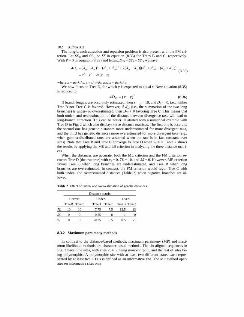
Tree B nor Tree C is favored. However, if d13 (i.e., the summation of the two long branches) is under- or overestimated, then DSS > 0 favoring Tree C. This means that both under- and overestimation of the distance between divergence taxa will lead to long-branch attraction. This can be better illustrated with a numerical example with Tree D in Fig. 2 which also displays three distance matrices. The first one is accurate, the second one has genetic distances more underestimated for more divergent taxa, and the third has genetic distances more overestimated for more divergent taxa (e.g., when gamma-distributed rates are assumed when the rate is in fact constant over sites). Note that Tree B and Tree C converge to Tree D when x5 = 0. Table 2 shows the results by applying the ME and LS criterion in analyzing the three distance matri-ces.
When the distances are accurate, both the ME criterion and the FM criterion re-covers Tree D (the true tree) with x5 = 0, TL = 10, and SS = 0. However, ME criterion favors Tree C when long branches are underestimated, and Tree B when long branches are overestimated. In contrast, the FM criterion would favor Tree C with both under- and overestimated distances (Table 2) when negative branches are al-lowed.
Table 2. Effect of under- and over-estimation of genetic distances
Distance matrix Correct Under- Over- TreeB TreeC TreeB TreeC TreeB TreeCTL 10 10 7.75 7.5 12.5 13SS 0 0 0.25 0 1 0x5 0 0 -0.25 0.5 0.5 -1
8.3.2 Maximum parsimony methods
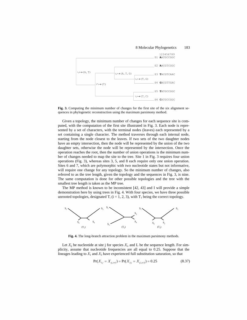
In contrast to the distance-based methods, maximum parsimony (MP) and maxi-mum likelihood methods are character-based methods. The six aligned sequences in Fig. 3 have nine sites, with sites 2, 4, 9 being monomorphic, and the rest of sites be-ing polymorphic. A polymorphic site with at least two different states each repre-sented by at least two OTUs is defined as an informative site. The MP method oper-ates on informative sites only.
8 Molecular Phylogenetics 183
S6 CATGCCGGC
S5 TATGCCGGC
S4 GACGTTGAC
S3 TACGTCAAC
S2 AACGTCGGC
S1 AATGCCGGC
∪→(T,C)
∪→(A,T)
∩→(T)
∪→(A,T,G)
∪→(T,G)
123456789
Fig. 3. Computing the minimum number of changes for the first site of the six alignment se-quences in phylogenetic reconstruction using the maximum parsimony method.
Given a topology, the minimum number of changes for each sequence site is com-puted, with the computation of the first site illustrated in Fig. 3. Each node is repre-sented by a set of characters, with the terminal nodes (leaves) each represented by a set containing a single character. The method traverses through each internal node, starting from the node closest to the leaves. If two sets of the two daughter nodes have an empty intersection, then the node will be represented by the union of the two daughter sets, otherwise the node will be represented by the intersection. Once the operation reaches the root, then the number of union operations is the minimum num-ber of changes needed to map the site to the tree. Site 1 in Fig. 3 requires four union operations (Fig. 3), whereas sites 3, 5, and 8 each require only one union operation. Sites 6 and 7, which are polymorphic with two nucleotide states but not informative, will require one change for any topology. So the minimum number of changes, also referred to as the tree length, given the topology and the sequences in Fig. 3, is nine. The same computation is done for other possible topologies and the tree with the smallest tree length is taken as the MP tree.
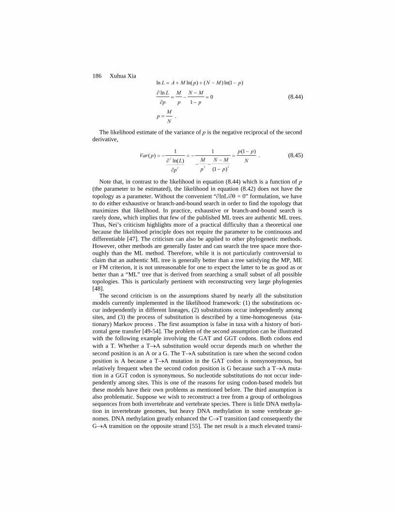
The MP method is known to be inconsistent [42, 43] and I will provide a simple demonstration here by using trees in Fig. 4. With four species, we have three possible unrooted topologies, designated Ti (i = 1, 2, 3), with T1 being the correct topology.
S1
S2
S3
S4
S1
S3
S2
S4
S1
S4
S3
S2
(T1) (T2) (T3)
Fig. 4. The long-branch attraction problem in the maximum parsimony methods.
Let Xij be nucleotide at site j for species Xi, and L be the sequence length. For sim-plicity, assume that nucleotide frequencies are all equal to 0.25. Suppose that the lineages leading to X1 and X3 have experienced full substitution saturation, so that
1 , 1 3 , 3Pr( ) Pr( ) 0.25j ij i j ij iX X X X≠ ≠= = = = (8.37)

184 Xuhua Xia where Pr stands for probability. The lineages leading to X2 and X4 have not experi-enced substitution saturation and have
2 4Pr( )j jX X P= = (8.38)
where P > 0.25. For simplicity, let us set P = 0.8, and L = 1000. We now consider the expected number of informative sites, designated by ni (i = 1,
2, 3), favoring Ti. By definition, site j is informative and favoring T1 if it meets the following three conditions: X1j = X2j, X3j = X4j, X1j ≠ X3j. Similarly, site j favors T2 if X1j = X3j, X2j = X4j, X1j ≠ X2j. Thus, the expected numbers of informative sites favoring T1, T2 and T3, respectively, are
1 1 2 3 4 1 3
2 1 3 2 4 1 2
3 1
( ) Pr( , , )
0.25 0.25 0.75 1000 47
( ) Pr( , , )
0.25 0.8 0.75 1000 150
( ) ( ) 47 .
j j j j j j
j j j j j j
E n X X X X X X L
E n X X X X X X L
E n E n
= = = ≠
= × × × ≈
= = = ≠
= × × × =
= ≈
(8.39)
The equations mean that, in spite of T1 being the true topology, we should have, on average, only about 47 informative sites favoring T1 and T3, but 150 sites supporting the wrong tree T2. This is one of the several causes for the familiar problem of long-branch attraction [44] or short-branch attraction [45]. Because it is the two short branches that contribute a large number of informative sites supporting the wrong tree, “short-branch attraction” seems a more appropriate term for the problem than “long-branch attraction”.
8.3.3 Maximum likelihood methods
The maximum likelihood (ML) method is based on explicit substitution models. Many different types of computer simulation have demonstrated the superiority of the ML method in recovering the true tree. I now use the four aligned sequences in Fig. 5 to illustrate numerically the computation involved in the ML method based on the JC69 model. With four sequences, we have three possible unrooted topologies of which one is shown in Fig. 5.
S1:A S3:G
S2:A S4:G65
t1t2
t3t4
t5
16
L1 = prob. + prob. + ... +
AAGG
C
A
AAGG
T
T
AAGG
A
AS1 ACATACGTS2 ACATACGTS3 GTCGACGTS4 GTCGACGT
Fig. 5. Likelihood calculation for the first site of the four aligned sequences.
The sequences have 8 sites, with the first four sites sharing one site pattern and the last four sites sharing another site pattern. So we need only two site-specific likeli-hood functions. The likelihood function of the first site, given the topology in Fig. 5, is the summation of the 16 probabilities corresponding to the 16 nucleotide combina-tions of the two internal nodes with unknown nucleotides (Fig. 5). Thus, the likeli-hood of the first site is,

8 Molecular Phylogenetics 185
1 2 5 3 4
1 2 5 3 4
1 2 5 3 4
1 . . . . .
. . . . .
. . . . .
...
A AA t AA t AA t AG t AG t
C CA t CA t CA t AG t AG t
T TA t TA t TT t TG t TG t
L P P P P P
P P P P P
P P P P P
π
π
π
=
+
++
(8.40)
where Pij.t for the JC69 model has already been given in equation (8.6) except that “8αt” should be replaced by “4αt”. Note that L2 = L3 = L4 =L1. We can write L5 (= L6 = L7 = L8) in a similar fashion.
The sequences in Fig. 5 allow us to simplify equation (8.40) greatly. Note that S1 = S2 and S3 = S4 (Fig. 5) so that αt1, αt2, αt3, and αt4 are all zero. Now we have
5
5
41
45
0.0625 0.0625
0.0625 0.1875 .
t
t
L e
L e
α
α
−
−
= −
= + (8.41)
With the assumption that all sites evolve independently, the likelihood function for
all eight sites is simply
5 5
4 41 5
1 5
4 4
ln 4ln( ) 4 ln( )
4 ln(0.0625 0.0625 ) 4ln(0.0625 0.1875 ) .t t
L L L
L L L
e eα α− −
=
= +
= − + +
(8.42)
The αt5 value that maximizes lnL is 0.27465, which leads to lnL = -21.02998. The
branch length between nodes 5 and 6 is 3αt5 = 0.82396. We can do the same calcula-tion for the other two possible topologies, and then choose the tree with the largest lnL value as the ML tree. In this particular example, the tree in Fig. 5 is the ML tree because it has the lnL value greater than that of the other two trees. One may also find that the ML tree, including its estimated branch lengths, is identical to the tree from a distance-based method such as the neighbor-joining [34], the FastME [36] or the Fitch-Margoliash method [35] as long as the JC69 distance is used.
There are two major criticisms on the ML method in phylogenetics. The first is that the application of the likelihood in phylogenetics is not really a ML method in its conventional sense because the topology is not in the likelihood function [3, 46]. To see this point, we can illustrate the conventional ML method with a simple example.
Suppose we wish to estimate the proportion of males (p) of a fish population in a large lake. A random sample of N fish contains M males. With the binomial distribu-tion, the likelihood function is
!
(1 ) .!( )!
M N MNL p p
M N M−= −
− (8.43)
The maximum likelihood method finds the value of p that maximizes the likeli-hood value. This maximization process is simplified by maximizing the natural loga-rithm of L instead:
186 Xuhua Xia
ln ln( ) ( ) ln(1 )
ln0
1
.
L A M p N M p
L M N M
p p p
Mp
N
= + + − −
∂ −= − =
∂ −
=
(8.44)
The likelihood estimate of the variance of p is the negative reciprocal of the second derivative,
2
2 22
1 1 (1 )( ) .
ln( )(1 )
p pVar p
M N ML Np pp
−= − = − =
−∂ − −−∂
(8.45)
Note that, in contrast to the likelihood in equation (8.44) which is a function of p (the parameter to be estimated), the likelihood in equation (8.42) does not have the topology as a parameter. Without the convenient “∂lnL/∂θ = 0” formulation, we have to do either exhaustive or branch-and-bound search in order to find the topology that maximizes that likelihood. In practice, exhaustive or branch-and-bound search is rarely done, which implies that few of the published ML trees are authentic ML trees. Thus, Nei’s criticism highlights more of a practical difficulty than a theoretical one because the likelihood principle does not require the parameter to be continuous and differentiable [47]. The criticism can also be applied to other phylogenetic methods. However, other methods are generally faster and can search the tree space more thor-oughly than the ML method. Therefore, while it is not particularly controversial to claim that an authentic ML tree is generally better than a tree satisfying the MP, ME or FM criterion, it is not unreasonable for one to expect the latter to be as good as or better than a “ML” tree that is derived from searching a small subset of all possible topologies. This is particularly pertinent with reconstructing very large phylogenies [48].
The second criticism is on the assumptions shared by nearly all the substitution models currently implemented in the likelihood framework: (1) the substitutions oc-cur independently in different lineages, (2) substitutions occur independently among sites, and (3) the process of substitution is described by a time-homogeneous (sta-tionary) Markov process . The first assumption is false in taxa with a history of hori-zontal gene transfer [49-54]. The problem of the second assumption can be illustrated with the following example involving the GAT and GGT codons. Both codons end with a T. Whether a T→A substitution would occur depends much on whether the second position is an A or a G. The T→A substitution is rare when the second codon position is A because a T→A mutation in the GAT codon is nonsynonymous, but relatively frequent when the second codon position is G because such a T→A muta-tion in a GGT codon is synonymous. So nucleotide substitutions do not occur inde-pendently among sites. This is one of the reasons for using codon-based models but these models have their own problems as mentioned before. The third assumption is also problematic. Suppose we wish to reconstruct a tree from a group of orthologous sequences from both invertebrate and vertebrate species. There is little DNA methyla-tion in invertebrate genomes, but heavy DNA methylation in some vertebrate ge-nomes. DNA methylation greatly enhanced the C→T transition (and consequently the G→A transition on the opposite strand [55]. The net result is a much elevated transi-

8 Molecular Phylogenetics 187 tion/transversion bias and increased AT% in the lineages with DNA methylation, violating the third assumption.
More complicated models have been proposed in response to our increased knowl-edge of the substitution process. However, such parameter-rich models require more data for reliable parameter estimation. The dilemma is that increasing the sequence length also increases the heterogeneity of substitution processes [56] including het-erotachy [57] operating on different sequence segments and consequently increase the number of parameters to be estimated. Such heterogeneity over sites implies that the consistency of the ML method [47, 58] is not of much value because we cannot get long sequences for a fixed and small number of parameters. Take for example the estimation of the proportion of male fish in the lake. If we get only six male fish in a sample with no female, then the likelihood estimation of p is 1 which is worse than our wildest guess without any data.
8.3.4 Bayesian inference
The Bayesian approach has only recently been used in phylogenetic inference [9]. Here I illustrate the basic principle of the Bayesian approach by using the problem of estimating the proportion (p) of males when the sample of six fish being all males. For a continuous variable such as p, the Bayes’ theorem is
( | ) ( )
( | )( | ) ( )
f y ff y
f y f d
θ θθ
θ θ θ=∫
(8.46)
where θ is the parameter of interest, y is the observed sample data, f(θ) is the prior probability for incorporating our prior knowledge on θ, f(y|θ) is the likelihood, and f(θ|y) is the posterior probability. In practice, equation (8.46) is rarely used because the integration in the denominator is difficult unless f(θ) and f(y|θ) are very simple, although the MCMC (Markov chain Monte Carlo) approach [59, 60] can alleviate the problem. Two alternative approaches have been devised to ease the computation burden, one being to use discrete approximations to continuous probability models, and the other being to use the conjugate prior distributions. For our example involv-ing a stationary and independent Bernoulli process in estimating p, the conjugate prior distribution is the beta distribution with the following f(p):
1 1( 1)!( ) (1 ) .( 1)!( 1)!
r n rnf p p pr n r
− − −−= −
− − − (8.47)
Let’s designate n and r as as n’ and r’ in the prior distribution, n” and r” in the pos-
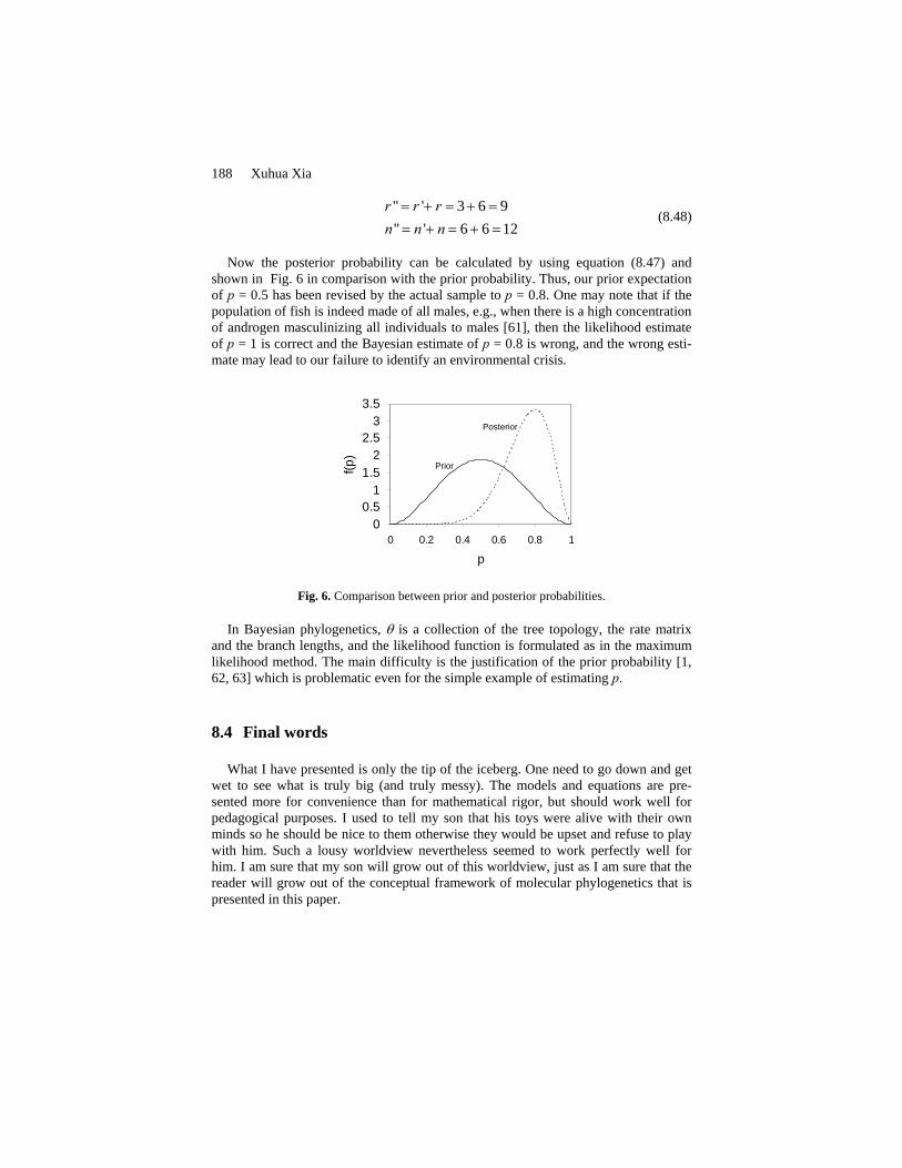
terior distribution, and just as n and r in the sample. If we expect the fish species to have equal number of males and females, then for a sample of six fish (n’ = 6), we expect r’ to be 3. The prior probability can be calculated from equation (8.47) and shown in Fig. 6.
It can be proven that, if the prior distribution of p is a beta distribution, then the posterior distribution will also be a beta distribution with the two parameters com-puted according to Eq. (8.48) below. In our actual sample with six males and 0 fe-male (n = 6 and r = 6),
188 Xuhua Xia
" ' 3 6 9" ' 6 6 12
r r rn n n= + = + == + = + =
(8.48)
Now the posterior probability can be calculated by using equation (8.47) and
shown in Fig. 6 in comparison with the prior probability. Thus, our prior expectation of p = 0.5 has been revised by the actual sample to p = 0.8. One may note that if the population of fish is indeed made of all males, e.g., when there is a high concentration of androgen masculinizing all individuals to males [61], then the likelihood estimate of p = 1 is correct and the Bayesian estimate of p = 0.8 is wrong, and the wrong esti-mate may lead to our failure to identify an environmental crisis.
00.5
11.5
22.5
33.5
0 0.2 0.4 0.6 0.8 1
p
f(p)
Prior
Posterior
Fig. 6. Comparison between prior and posterior probabilities.
In Bayesian phylogenetics, θ is a collection of the tree topology, the rate matrix and the branch lengths, and the likelihood function is formulated as in the maximum likelihood method. The main difficulty is the justification of the prior probability [1, 62, 63] which is problematic even for the simple example of estimating p.
8.4 Final words
What I have presented is only the tip of the iceberg. One need to go down and get wet to see what is truly big (and truly messy). The models and equations are pre-sented more for convenience than for mathematical rigor, but should work well for pedagogical purposes. I used to tell my son that his toys were alive with their own minds so he should be nice to them otherwise they would be upset and refuse to play with him. Such a lousy worldview nevertheless seemed to work perfectly well for him. I am sure that my son will grow out of this worldview, just as I am sure that the reader will grow out of the conceptual framework of molecular phylogenetics that is presented in this paper.
8 Molecular Phylogenetics 189 Acknowledgements
I thank S. Aris-Brosou, B. Golding, D. Hickey, A. Meyer, S. Kumar, J. R. Lobry, D. Sankoff, and H. Xiong for comments, suggestions and corrections, and NSERC Discovery, RTI and Strategic grants for funding.
References
1. Felsenstein J.: Inferring phylogenies. Sinauer, Sunderland, Massachusetts (2004)
2. Li W.-H.: Molecular evolution. Sinauer, Sunderland, Massachusetts (1997) 3. Nei M., Kumar S.: Molecular evolution and phylogenetics. Oxford University
Press, New York (2000) 4. Kumar S., Tamura K., Jakobsen I.B., Nei M.: MEGA2: molecular evolutionary
genetics analysis software. Bioinformatics, 17(2001) 1244-1245 5. Swofford D.L.: Phylogeentic analysis using parsimony (* and other methods), 4
edn. Sinauer, Sunderland, Mass. (2000) 6. Xia X., Xie Z.: DAMBE: Software package for data analysis in molecular biol-
ogy and evolution. J Hered, 92(2001) 371-373 7. Xia X.: Data analysis in molecular biology and evolution. Kluwer Academic
Publishers, Boston (2001) 8. Yang Z.: Phylogenetic analysis by maximum likelihood (PAML). Version 3.12.
University College, London. (2002) 9. Huelsenbeck J.P., Ronquist F., Nielsen R., Bollback J.P.: Bayesian inference of
phylogeny and its impact on evolutionary biology. Science, 294(2001) 2310-2314.
10. Jukes T.H., Cantor C.R.: Evolution of protein molecules. In: Mammalian protein metabolism. Edited by Munro HN. Academic Press, New York (1969): 21-123
11. Kimura M.: A simple method for estimating evolutionary rates of base substitu-tions through comparative studies of nucleotide sequences. J Mol Evol, 16(1980) 111-120
12. Tamura K., Nei M.: Estimation of the number of nucleotide substitutions in the control region of mitochondrial DNA in humans and chimpanzees. Mol Biol Evol, 10(1993) 512-526
13. Kimura M., Ohta T.: On the stochastic model for estimation of mutational dis-tance between homologous proteins. J Mol Evol, 2(1972) 87-90
14. Tamura K., Kumar S.: Evolutionary distance estimation under heterogeneous substitution pattern among lineages. Mol Biol Evol, 19(2002) 1727-1736.
15. Huelsenbeck J.P., Larget B., Alfaro M.E.: Bayesian phylogenetic model selec-tion using reversible jump Markov chain Monte Carlo. Mol Biol Evol, 21(2004) 1123-1133
16. Lake J.A.: Reconstructing evolutionary trees from DNA and protein sequences: paralinear distances. Proc Natl Acad Sci USA, 91(1994) 1455-1459
17. Lockhart P.J., Steel M.A., Hendy M.D., Penny D.: Recovering evolutionary trees under a more realistic model of sequence evolution. Mol Biol Evol, 11(1994) 605-612

190 Xuhua Xia 18. Rosenberg M.S., Kumar S.: Heterogeneity of nucleotide frequencies among
evolutionary lineages and phylogenetic inference. Mol Biol Evol, 20(2003) 610-621
19. Xia X.: Phylogenetic Relationship among Horseshoe Crab Species: The Effect of Substitution Models on Phylogenetic Analyses. Syst Biol, 49(2000) 87-100
20. Xia X.H., Xie Z., Kjer K.M.: 18S ribosomal RNA and tetrapod phylogeny. Syst Biol, 52(2003) 283-295
21. Adachi J., Hasegawa M.: Model of amino acid substitution in proteins encoded by mitochondrial DNA. J Mol Evol, 42(1996) 459-468
22. Kishino H., Miyata T., Hasegawa M.: Maximum likelihood inference of protein phylogeny and the origin of chloroplasts. J Mol Evol, 31(1990) 151-160
23. Dayhoff M.O., Schwartz R.M., Orcutt B.C.: A model of evolutionary change in proteins. In: Atlas of Protein Sequence and Structure. Edited by Dayhoff MO, vol. 5, Suppl. 3. National Biomedical Research Foundation, Washington D.C. (1978): 345-352
24. Jones D.T., Taylor W.R., Thornton J.M.: The rapid generation of mutation data matrices from protein sequences. Comput Appl Biosci, 8(1992) 275-282.
25. Xia X., Li W.H.: What amino acid properties affect protein evolution? J Mol Evol, 47(1998) 557-564.
26. Xia X., Xie Z.: Protein structure, neighbor effect, and a new index of amino acid dissimilarities. Mol Biol Evol, 19(2002) 58-67
27. Goldman N., Yang Z.: A codon-based model of nucleotide substitution for pro-tein-coding DNA sequences. Mol Biol Evol, 11(1994) 725-736
28. Muse S.V., Gaut B.S.: A likelihood approach for comparing synonymous and nonsynonymous nucleotide substitution rates, with application to the chloroplast genome. Mol Biol Evol, 11(1994) 715-724
29. Yang Z., Nielsen R.: Estimating synonymous and nonsynonymous substitution rates under realistic evolutionary models. Mol Biol Evol, 17(2000) 32-43.
30. Xia X.: Maximizing transcription efficiency causes codon usage bias. Genetics, 144(1996) 1309-1320
31. Xia X.: How optimized is the translational machinery in Escherichia coli, Sal-monella typhimurium and Saccharomyces cerevisiae? Genetics, 149(1998) 37-44.
32. Xia X.: Mutation and Selection on the Anticodon of tRNA Genes in Vertebrate Mitochondrial Genomes. Gene, 345(2005) 13-20
33. Ikemura T.: Correlation between codon usage and tRNA content in microorgan-isms. In: Transfer RNA in protein synthesis. Edited by Hatfield DL, Lee B, Pir-tle J. CRC Press, Boca Raton, Fla. (1992): 87-111
34. Saitou N., Nei M.: The neighbor-joining method: a new method for reconstruct-ing phylogenetic trees. Mol Biol Evol, 4(1987) 406-425
35. Fitch W.M., Margoliash E.: Construction of phylogenetic trees. Science, 155(1967) 279-284
36. Desper R., Gascuel O.: Fast and accurate phylogeny reconstruction algorithms based on the minimum-evolution principle. J Comput Biol, 9(2002) 687-705.
37. Xia X.H., Xie Z., Salemi M., Chen L., Wang Y.: An index of substitution satu-ration and its application. Mol Phylogenet Evol, 26(2003) 1-7
38. Golding G.B.: Estimates of DNA and protein sequence divergence: An exami-nation of some assumptions. Mol Biol Evol, 1(1983) 125-142

8 Molecular Phylogenetics 191 39. Nei M., Gojobori T.: Simple methods for estimating the numbers of synony-
mous and nonsynonymous nucleotide substitutions. Mol Biol Evol, 3(1986) 418-426
40. Jin L., Nei M.: Limitations of the evolutionary parsimony method of phyloge-netic analysis. Mol Biol Evol, 7(1990) 82-102
41. Waddell P.J.: Statistical methods of phylogenetic analysis: including Hadamard conjugations, LogDet transforms, and maximum likelihood. Ph.D. thesis. Massey University, New Zealand (1995)
42. Felsenstein J.: Cases in which parsimony and compatibility methods will be positively misleading. Syst Zool, 27(1978) 401-410
43. Takezaki N., Nei M.: Inconsistency of the maximum parsimony method when the rate of nucleotide substitution is constant. J Mol Evol, 39(1994) 210-218.
44. Hendy M.D., Penny D.: A framework for the quantitative study of evolutionary trees. Syst Zool, 38(1989) 297-309
45. Nei M.: Phylogenetic analysis in molecular evolutionary genetics. Annu Rev Genet, 30(1996) 371-403
46. Nei M.: Molecular Evolutionary Genetics. Columbia University Press, New York (1987)
47. Chang J.T.: Full reconstruction of Markov models on evolutionary trees: identi-fiability and consistency. Math Biosci, 137(1996) 51-73.
48. Tamura K., Nei M., Kumar S.: Prospects for inferring very large phylogenies by using the neighbor-joining method. Proc Natl Acad Sci U S A, 101(2004) 11030-11035
49. Medigue C., Rouxel T., Vigier P., Henaut A., Danchin A.: Evidence for hori-zontal gene transfer in Escherichia coli speciation. J Mol Biol, 222(1991) 851-856
50. Koonin E.V.: Horizontal gene transfer: the path to maturity. Mol Microbiol, 50(2003) 725-727
51. Philippe H., Douady C.J.: Horizontal gene transfer and phylogenetics. Curr Opin Microbiol, 6(2003) 498-505
52. Kurland C.G., Canback B., Berg O.G.: Horizontal gene transfer: a critical view. Proc Natl Acad Sci U S A, 100(2003) 9658-9662
53. Brown J.R.: Ancient horizontal gene transfer. Nat Rev Genet, 4(2003) 121-132 54. Eisen J.A.: Horizontal gene transfer among microbial genomes: new insights
from complete genome analysis. Curr Opin Genet Dev, 10(2000) 606-611 55. Xia X.H.: DNA methylation and mycoplasma genomes. J Mol Evol, 57(2003)
S21-S28 56. Xia X.: The rate heterogeneity of nonsynonymous substitutions in mammalian
mitochondrial genes. Mol Biol Evol, 15(1998) 336-344 57. Kolaczkowski B., Thornton J.W.: Performance of maximum parsimony and
likelihood phylogenetics when evolution is heterogeneous. Nature, 431(2004) 980-984
58. Felsenstein J.: Phylogenies from molecular sequences: inference and reliability. Annu Rev Genet, 22(1988) 521-565
59. Hastings W.K.: Monte Carlo sampling methods using Markov chain and their applications. Biometrika, 57(1970) 97-109
60. Metropolis N., Rosenbluth A.W., Rosenbluth M.N., Teller A.H., Teller E.: Equation of state calculations by fast computing machines. J Chem Phys, 21(1953) 1087-1092

192 Xuhua Xia 61. Baron D., Cocquet J., Xia X., Fellous M., Guiguen Y., Veitia R.A.: An evolu-
tionary and functional analysis of FoxL2 in rainbow trout gonad differentiation. J Mol Endocrinol, 33(2004) 705 - 715
62. Zwickl D., Holder M.: Model parameterization, prior distributions, and the gen-eral time-reversible model in Bayesian phylogenetics. Syst Biol, 53(2004) 877-888
63. Pickett K.M., Randle C.P.: Strange bayes indeed: uniform topological priors imply non-uniform clade priors. Mol Phylogenet Evol, 34(2005) 203-211