prism local model validation report -...
TRANSCRIPT

PRISM Local Model Validation Report
PRISM 4.5
February 2017
PRISM Management Group


370745 ITD 1 A
http://pims01/pims/llisapi.dll/open/1557091063
June 2016
PRISM Local Model Validation Report
PRISM 4.5
PRISM Local Model Validation Report
PRISM 4.5
February 2017
PRISM Management Group


Mott MacDonald, 35 Newhall Street, Birmingham, B3 3PU, United Kingdom
T +44 (0)121 234 1500 F +44 (0)121 200 3295 W www.mottmac.com

PRISM Local Model Validation Report PRISM 4.5
370745/ITD//1/A February 2017 "PRISM 4.5 Reports-1.Local Model Validation Report-6.docx"
Revision Date Originators Checker Approver Description
1
10/09/2014
Stacey Luxton Mike Oliver Jevgenija Guliajeva Nick Taylor
Tim Slater (Centro, PT sections) Mike Oliver
Philip Old
First issue
2
12/01/2015
Jevgenija Guliajeva Nick Taylor
Tim Slater (Centro, PT sections) Tim Day-Pollard
Philip Old
First issue
3
30/04/2015
Jevgenija Guliajeva Nick Taylor
Tim Slater (Centro, PT sections) Tim Day-Pollard
Philip Old
First issue
4 19/10/2016 Tim Day-Pollard Duncan Lockwood
Duncan Lockwood
PRISM v4.5
5 15/12/2016 Tim Day-Pollard Duncan Lockwood
Duncan Lockwood
PRISM v4.5 – internal review – then passing to client review.
6 22/02/2017 James Edwards (Vectos)
Tim Day-Pollard Post client review
Issue and revision record
This document is issued for the party which commissioned it and for specific purposes connected with the above-captioned project only. It should not be relied upon by any other party or used for any other purpose.
We accept no responsibility for the consequences of this document being relied upon by any other party, or being used for any other purpose, or containing any error or omission which is due to an error or omission in data supplied to us by other parties.
This document contains confidential information and proprietary intellectual property. It should not be shown to other parties without consent from us and from the party which commissioned it.

PRISM Local Model Validation Report PRISM 4.5
370745/ITD//1/A February 2017 "PRISM 4.5 Reports-1.Local Model Validation Report-6.docx"
PRISM Local Model Validation Report PRISM 4.5
370745/ITD//1/A February 2017 "PRISM 4.5 Reports-1.Local Model Validation Report-6.docx"
Chapter Title Page
Glossary and Abbreviations iii
Executive Summary v
1 Introduction 9
1.1 Overview _________________________________________________________________________ 9 1.2 Uses of the Model _________________________________________________________________ 10
2 Highway 12
2.1 Model Standards __________________________________________________________________ 12 2.2 Key Features _____________________________________________________________________ 14 2.3 Calibration/Validation Data ___________________________________________________________ 25 2.4 Network _________________________________________________________________________ 27 2.5 Trip Matrix _______________________________________________________________________ 33 2.6 Calibration/Validation _______________________________________________________________ 44 2.7 Summary ________________________________________________________________________ 63
3 Public Transport 64
3.1 Model Standards __________________________________________________________________ 64 3.2 Key Features in PRISM 4.5 __________________________________________________________ 64 3.3 Key Features _____________________________________________________________________ 67 3.4 Calibration Data ___________________________________________________________________ 75 3.5 Network _________________________________________________________________________ 77 3.6 Trip Matrix _______________________________________________________________________ 78 3.7 Calibration/Validation _______________________________________________________________ 85 3.8 Summary ________________________________________________________________________ 94
4 Variable Demand Model 95
4.1 Key Features _____________________________________________________________________ 95 4.2 Demand Model ____________________________________________________________________ 96 4.3 Planning Data ____________________________________________________________________ 102 4.4 Realism Testing __________________________________________________________________ 114 4.5 Summary _______________________________________________________________________ 116
5 Summary 117
5.1 Model Development _______________________________________________________________ 117 5.2 Standards Achieved _______________________________________________________________ 117
Appendices 118
Contents

PRISM Local Model Validation Report PRISM 4.5
ii 370745/ITD//1/A February 2017 "PRISM 4.5 Reports-1.Local Model Validation Report-6.docx"

PRISM Local Model Validation Report PRISM 4.5
iii 370745/ITD//1/A February 2017 "PRISM 4.5 Reports-1.Local Model Validation Report-6.docx"
Term Description
Area of Detailed Modelling (AoDM) This area is modelled in detail, hence characterised by representation of all trip movements, small zones, detailed networks and junction modelling
ATC Automatic Traffic Count
Calibration Adjustments to the model intended to reduce the differences between the modelled and observed data.
Capacity ratio Total upstream demand divided by the flow/capacity of the downstream link.
Cruise speed The mid-link speed, separate from any junction delay, during the time period modelled.
Demand model A model which forecasts the demand for travel in terms of trip frequency, mode of travel, time of travel, park and ride station choice and trip destination.
DfT Department for Transport
External area The area outside the Fully Modelled Area.
Flow/delay relationship The relationship between traffic flow and travel time along a link or turn, sometimes adjusted to allow for non-transient queues and flow metering.. This is also known as a speed/flow relationship.
Fully Modelled area (FMA) The area where trip matrices are complete (as opposed to partial in the External Area) and the network and zoning are at their most detailed.
HE Highways England (formerly Highways Agency – HA)
HATRIS Highways Agency Traffic Information System
HI Household Interview
Highway Assignment Model (HAM) A model which allocates car and goods vehicle trips to routes through a highway network. It includes path building and loading of trips to routes between zones. It excludes all demand responses other than route choice.
ICA Intersection Capacity Analysis (in Visum)
IDBR Inter Departmental Business Register
LMVR Local Model Validation Report
Matrix estimation The adjustment of prior trip matrices so that, when assigned, the resulting flows accord more closely with counts used as constraints in the process.
MCC Manual Classified Count
NTEM National Trip End Model
NTS National Travel Survey
OD Origin-Destination
PCU Passenger Car Unit
Planet Framework Model This is a strategic UK model that has been developed for HS2 Ltd and the DfT. Long distance rail demand is forecast in the (sub) model known as Planet Long distance. A full model description is available: https://www.gov.uk/government/publications/planet-framework-model-pfm-v43-model-description
PLD Planet Long Distance
PMG PRISM Management Group
PRISM Policy Responsive Integrated Strategy Model
PRISM Refresh Version 4.1 of PRISM
PT Public Transport
Glossary and Abbreviations

PRISM Local Model Validation Report PRISM 4.5
iv 370745/ITD//1/A February 2017 "PRISM 4.5 Reports-1.Local Model Validation Report-6.docx"
Term Description
Public Transport Assignment Model (PTAM)
A model which allocates public transport passenger trips to routes through a public transport network. It includes path building and loading of trips to routes between zones. It excludes all demand responses other than change of route and service.
Rest of the Fully Modelled Area (RotFMA) The area over which the impacts of interventions are considered to be quite likely but relatively weak in magnitude.
RSI Road Side Interview
TLD Trip Length Distributions
TM Trafficmaster
TRADS Traffic Flow Data System
Validation The comparison of modelled and observed data, where the observed data is independent from that used in calibration. Any adjustments to the model intended to reduce the differences between the modelled and observed data should be regarded as calibration.
VDF Volume Delay Function
VDM Variable Demand Model
Volume to capacity ratio Total upstream volume divided by the capacity of the downstream link.
VoT Value of Time
WebTAG DfT online Transport Analysis Guidance
WM West Midlands
WMMA West Midlands Metropolitan Area

PRISM Local Model Validation Report PRISM 4.5
v 370745/ITD//1/A February 2017 "PRISM 4.5 Reports-1.Local Model Validation Report-6.docx"
Background
The West Midlands’ Policy Responsive Integrated Strategy Model (PRISM) is a
multi-modal disaggregate demand model of the West Midlands Metropolitan Area.
The model comprises separate highway and Public Transport (PT) assignment
models linked together with a demand model. PRISM was originally developed to
represent a 2001 base and was later rebased to 2006. Following stakeholder
consultation, Mott MacDonald was commissioned by the PRISM Management
Group (PMG) to undertake a comprehensive update and to produce updated
highway and public transport models for a 2011 base year. That work culminated
in PRISM 4.1. Following subsequent application work a number of improvements
were identified and the PMG commissioned Mott MacDonald to produce an
updated model. This report documents the development of the 2011 base year
models, including the variable demand model for PRISM 4.5.
Key Features
The highway models represent an average weekday for three time periods; the
AM average hour from 0700 to 0930, the IP average hour from 0930 to 1530 and
the average PM hour from 1530 to 1900. Four user-classes are modelled; Car
Work, Car Non Work, LGV and HGV. The models use an equilibrium assignment
procedure that incorporates detailed junction modelling and blocking back within
the Area of Detailed Modelling.
The PT models represent an average weekday for three time periods; the AM
average hour from 0700 to 0900, the IP average hour from 1000 to 1200 and the
average PM hour from 1600 to 1800. Seven user-classes are modelled; “Bus-
Fare”, “Metro-Fare”, “Train-Fare”, “Bus-No Fare”, “Metro-No Fare”, “Train-No
Fare”, , and PLANET Long Distance. The assignment methodology makes use of
the timetable based assignment and parameters provided in the Visum 15
software.
The demand model consists of the following three main components: the
Population Model, the Travel Demand Model and the Final Processing Model. The
outcome of these three processes is a set of revised demand matrices for
Executive Summary
PRISM Local Model Validation Report PRISM 4.5
vi 370745/ITD//1/A February 2017 "PRISM 4.5 Reports-1.Local Model Validation Report-6.docx"
assignment in the HAM and PTAM. These new matrices include responses to cost
changes in the assignment model, as well as demographic changes.
Data Collection
A comprehensive data collection exercise was undertaken in the development of
the models. Data collected included Road Side Interviews, household travel
surveys, public transport user surveys, GPS data including Trafficmaster and
INRIX, NAVTEQ, automatic and manual traffic counts and journey time data.
Model Development
The 2011 base year highway and public transport networks were developed
based on the existing networks. Junction coding within the Area of Detailed
Modelling was reviewed and updated based on aerial photography, the Integrated
Transport Network (ITN), NAVTEQ and consultation with the PMG. The zoning
system was also updated, allowing for the disaggregation of certain zones to allow
for finer distribution of demand and for greater consistency with the PT
assignment model. The services within the public transport model were updated
based on ATCO-CIF data.
Model Calibration and Validation
The prior trip matrices were assigned to the highway and public transport
networks and comparisons of the outputs were made to observed data. A matrix
estimation process was then undertaken for different user-classes. Matrix
estimation is a process whereby non-zero matrix cell values are adjusted so that
modelled flows better match observed. The estimated matrices were then
assigned to the networks and compared against observations to assess the level
of validation and additionally for the highway model compared against observed
journey times.
Individual comparisons show that the models produce base year traffic flows and
passenger demand consistent with those observed. Trip length distribution
comparisons show that matrix estimation has had little effect on mean trip lengths.
PRISM Local Model Validation Report PRISM 4.5
vii 370745/ITD//1/A February 2017 "PRISM 4.5 Reports-1.Local Model Validation Report-6.docx"
The response of the PRISM variable demand model to changes in car fuel cost,
public transport fares and car journey time is realistic, albeit slightly outside the
recommended WebTAG ranges in some cases. The relative elasticities within
each test between demand segments is also realistic, suggesting PRISM is a
robust model for forecasting the travel demand patterns of the West Midlands
population.
The calibration process produced a model that closely fits observed link traffic flow
and journey time observations.

PRISM Local Model Validation Report PRISM 4.5
viii
370745/ITD//1/A February 2017 "PRISM 4.5 Reports-1.Local Model Validation Report-6.docx"

"PRISM 4.5 Reports-1.Local Model Validation Report-6.docx"
9
PRISM Local Model Validation Report
1.1 Overview
The Policy Responsive Integrated Strategy Model (PRISM) is a multi-modal disaggregate demand model of
the West Midlands Metropolitan Area. The model comprises both a highway and a public transport
assignment model linked with a demand model. The client is the seven Metropolitan districts of the West
Midlands, Highways England and Transport for West Midlands1.
PRISM was originally developed to represent a 2001 base year and was later rebased to 2006. In 2009
and 2010, Mott MacDonald (MM) consulted with a range of stakeholders including Metropolitan
Authorities, the Highways Agency, Shire Authorities, Department for Transport (DfT), West Midlands
Regional Assembly, Government Office for the West Midlands and Birmingham International Airport. A
range of issues were raised at this consultation. Mott MacDonald were commissioned to develop a 2011
base year model, addressing some of these issues such as including improved junction coding and a public
transport model for the PM peak. That work resulted in a new PRISM model (with 2011 base year), with
reporting finishing 15th May 2015. For the duration of the report that will be referred to as PRISM 4.1.
Where reference is made to work done on the PRISM Refresh, this can be interpreted as work done to
develop PRISM 4.1, and that little to no alterations were required for PRISM 4.5
Following on from subsequent application work, a number of improvements to the model system were
identified which led to the development of PRISM 4.5, briefly these can be summarised as:
PRISM 4.1 PT assignment were headway-based and used VISUM 12.5, which can lead to some
unrealistic cost changes between a do-minimum and do-something test scenario. In particular it was
found that sometimes network improvements produced output costs quantifiably worse which in turn
made scheme appraisal very difficult.
PRISM 4.5 is timetable-based and uses new functionality that we specifically requested in VISUM 15,
to address this issue
PRISM 4.5 demand model has been re-calibrated using more data to better represent sub-mode choice
between rail and metro.
PRISM 4.5 PT assignment demand is now segmented by PT sub-mode (bus, metro, rail)
PRISM 4.5 demand forecasts can now account for new park and ride (and kiss and ride) stations.
PRISM 4.5 highway assignment includes observed signal timings, which lead to more realistic delays.
PRISM 4.5 highway assignment convergence is much more stable, which is important for economic
appraisal. PRISM 4.5 base year matrices now include journey-to-work data derived from the 2011
census which had not been previously made available.
The PRISM 4.5 update was completed July 2016, reporting work has been delayed due to work on the PRISM 4.6 update.
This Local Model Validation Report (LMVR) describes the development of the PRISM 4.5 2011 base year
highway assignment and public transport (PT) model in detail, and presents the level of validation achieved
against observed traffic flow and journey time data.
The complete set of reporting for PRISM 4.5 should be interpreted as:
PRISM 4.5 – Local Model Validation Report (this report)
PRISM 4.5 – Forecasting Report
1 Formerly CENTRO
1 Introduction

"PRISM 4.5 Reports-1.Local Model Validation Report-6.docx"
10
PRISM Local Model Validation Report
PRISM 4.5 – Data Summary Report
Other PRISM reports of relevance are:
PRISM Refresh Technical Note 1: Zoning (Mott MacDonald, June 2012)
PRISM Refresh Technical Note 3: Highway Network Build (Mott MacDonald, December 2012)
Data collection:
PRISM Surveys 2011: Household Travel Survey (Mott MacDonald, November 2012)
PRISM Surveys 2011: Public Transport (Mott MacDonald, November 2012)
PRISM Surveys 2011: Roadside Interviews (Mott MacDonald, November 2012)
PRISM Surveys 2011: Urban Centres (Mott MacDonald, November 2012)
PRISM Demand Model:
PRISM 2011 Base: Mode-Destination Model Estimation (RAND Europe, 2014)
PRISM 2011 Base: Frequency and Car Ownership Models (RAND Europe, 2014)
PRISM 2011 Base: Demand Model Implementation (RAND Europe, 2014)
The highway assignment models have been developed in accordance with the DfT’s online Transport
Analysis Guidance (WebTAG), http://www.dft.gov.uk/webtag, and the Highways England (HE) Design
Manual for Roads and Bridges (DMRB) Volume 12, as well as Mott MacDonald internal best practice
guidelines.
The PRISM models have been developed using Visum software, version 15.00-14. The base year models
represent an average weekday in 2011 and have been developed to represent the average hour over three
time periods; AM, IP and PM. Within PRISM, three vehicle types have been modelled: car, light goods
vehicles and heavy goods vehicles. Levels of detail within the model differ by area, with detailed junction
coding in the Area of Detailed Modelling (AoDM). In total, the model consists of 994 zones; the majority of
which are contained in the West Midlands Metropolitan Area (WMMA). These key features of the model are
described in detail in section 2.2.
1.2 Uses of the Model
1.2.1 Scenarios and Interventions
PRISM was originally designed in 2001 and since its development in 2004 it has been used for a wide
range of applications. This has included support for the assessment of local development plans, major
scheme business cases, local models and as a database of travel and transport information. As a database
of travel movements, PRISM has provided input to more local models, including microsimulation.
As in the past, it is intended that future transport and land use planning projects in the West Midlands that
require modelling support will use PRISM, either as the database of network detail, planning data or travel
demand patterns, or as a fully functional tool. The database may be more useful for smaller scale studies,
for which cordoned networks and/or matrices can be generated for the standard model years 2011, 2021
and 2031, whilst the full model specification becomes more relevant when forecasting the impacts of
strategic transport schemes or substantial land use changes in the future. Additional model years can be
modelled, although this will require additional work.

"PRISM 4.5 Reports-1.Local Model Validation Report-6.docx"
11
PRISM Local Model Validation Report
1.2.2 Key Design Considerations
PRISM is the Strategic Transport Model for the West Midlands. The model’s geographical area, modal
representation, functional responsiveness and segmentation have been designed to reflect the intended
uses of the model which are:
To support development of local and regional transport and land use policies;
To support Major Scheme Business Cases;
To provide network inputs and consistent demand forecasts for local studies;
To be a database of travel demand data in the West Midlands Region;
To provide the Highways Agency with a robust regional modelling tool for projects and programmes in
the West Midlands; and
To support prioritisation of major schemes and economic impact studies.
The model’s design focuses on the above objectives, also recognising the investment in the original model
in 2001, consistency with results and assumptions previously made, and constraints imposed by software
and reducing funding budgets.
As part of the consultations of the PRISM Management Group (PMG) it was decided that for PRISM 4.1 a
new unified Public Transport model should be created alongside the PRISM HAM and that the PT model
should be made by taking elements from two previous models; the Centro 2005/2008 PT Model and the
PRISM 2006 PT Model. Where previously the models were used separately and could feed into each other
the ‘Unified’ model can be used separately by the relevant parties. PRISM 4.5 builds on from this model.
This provides many benefits:
The ability for parties to work separately, removing errors that occur from the exchange of data
between parties and between both models;
Greater accuracy of skims and route choice throughout the model;
Provision for Centro to use larger networks with a wider coverage;
A more detailed zoning system which means that users are fed more accurately onto the network than
previously;
The ability for more than one party to work together on the model, share skills and in turn reduce costs
to both parties; and
Provide an improvement in overall efficiency.

"PRISM 4.5 Reports-1.Local Model Validation Report-6.docx"
12
PRISM Local Model Validation Report
2.1 Model Standards
2.1.1 Model Validation Criteria and Acceptability Guidelines
For all elements of highway assignment validation, the validation criteria and acceptability guidelines used
are as stated in TAG M3.1, except where noted.
2.1.1.1 Trip Matrix Validation
For trip matrix validation, the measure used was the percentage difference between modelled flows and
observed counts. The criterion and acceptability guidelines for screenline flows are defined in Table 2.1.
Table 2.1: The acceptability guidelines for trip matrix validation
Criteria Acceptability guideline
Differences between modelled flows and counts should be less than 5% of the counts
All or nearly all screenlines
Source: WebTAG Unit M3.1 (Section 3.2.5, Table 1)
Screenlines have been split into three different types:
Roadside interview;
Other screenlines used in matrix calibration; and
Independent validation.
2.1.1.2 Link flow validation
For link flow validation, the measures used were:
The GEH statistic, which incorporates both relative and absolute errors; and
The absolute and percentage difference between modelled flows and observed counts.
The TAG Unit M3.1 criteria and acceptability guidelines for link flows are defined in Table 2.2.
Table 2.2: The WebTAG acceptability guidelines for individual link flow validation
Criteria Description of criteria Acceptability guideline
1 Individual flows within 100 vehicles/hour of counts for flows less than 700 vehicles/hour
>85% of cases
Individual flows within 15% of counts for flows from 700 to 2700 vehicles/hour >85% of cases
Individual flows within 400 vehicles/hour of counts for flows more than 2,700 vehicles/hour
>85% of cases
2 GEH < 5 for individual flows >85% of cases
Source: WebTAG Unit M3.1 (Section 3.2.8, Table 2)
2.1.1.3 Journey Time Validation
For journey time validation, the measure used is the percentage difference between modelled and
observed journey times, subject to an absolute maximum difference. The criteria and acceptability
2 Highway

"PRISM 4.5 Reports-1.Local Model Validation Report-6.docx"
13
PRISM Local Model Validation Report
guidelines for journey times are defined in Table 2.3. WebTAG Unit M3.1 indicates that journey time routes
should be between 3km and 15km.
Table 2.3: The acceptability guidelines for journey time validation
Criteria Acceptability guideline
Modelled times along routes should be within 15% of surveyed times (or 1 minute)
>85% of cases
Source: WebTAG Unit M3.1(Section 3.2.10, Table 3)
2.1.2 Convergence Criteria
The highway assignment models use a procedure that includes a local user-cost equilibrium (LUCE)
assignment with blocking back and Intersection Capacity Analysis (ICA). Measures of convergence
monitored during assignment are provided in Table 2.4.
Table 2.4: Highway assignment convergence criteria
Description of test Acceptability guideline
Overall Assignment:
1 The link volumes from the current embedded assignment and the previous embedded assignment are close
More than 95% of links have a difference in delay less than GEH 1
2 The turn volumes from the current embedded assignment and the previous embedded assignment are close
More than 95% of turns have a difference in delay less than GEH 1
3 The turn volumes from the current embedded assignment and the “smoothed” turn volumes used in ICA close
More than 95% of turns have a difference in delay less than GEH 1
4 The final link delays from the embedded assignment and those obtained from running ICA/Blocking Back are close, i.e. testing if the link VDFs are a good estimate of delay
More than 90% of turns have a relative difference in delay less than 5%
5 The final turn delays from the embedded assignment and those obtained from running ICA/Blocking Back are close, i.e. testing if the turn VDFs are a good estimate of delay
More than 90% of turns have a relative difference in delay less than 5%
6 The mean deviation in queue lengths on links is sufficiently small i.e. the queues have stabilised.
Less than 1 vehicle
Embedded Assignment:
7 DELTA: The difference between the costs along the chosen routes and those along the minimum cost routes, summed across the whole network, and expressed as the percentage of the minimum costs (referred to as ‘delta’ in TAG unit M3-1 section C.2.4)
Less than 0.0001%
Source: PTV advice on Visum assignment with ICA
The above section details convergence criteria that were developed by PTV for Mott MacDonalds use of
PRISM (after much consultation between the two). This advice was formulated taking into consideration
experiences with the TfL One model, and also the need for reasonable run-times. For PRISM 4.1 a base
year assignment could easily take over 12 hours of runtime to reach those criteria.
"PRISM 4.5 Reports-1.Local Model Validation Report-6.docx"
14
PRISM Local Model Validation Report
2.2 Key Features
2.2.1 Fully Modelled Area and External Area
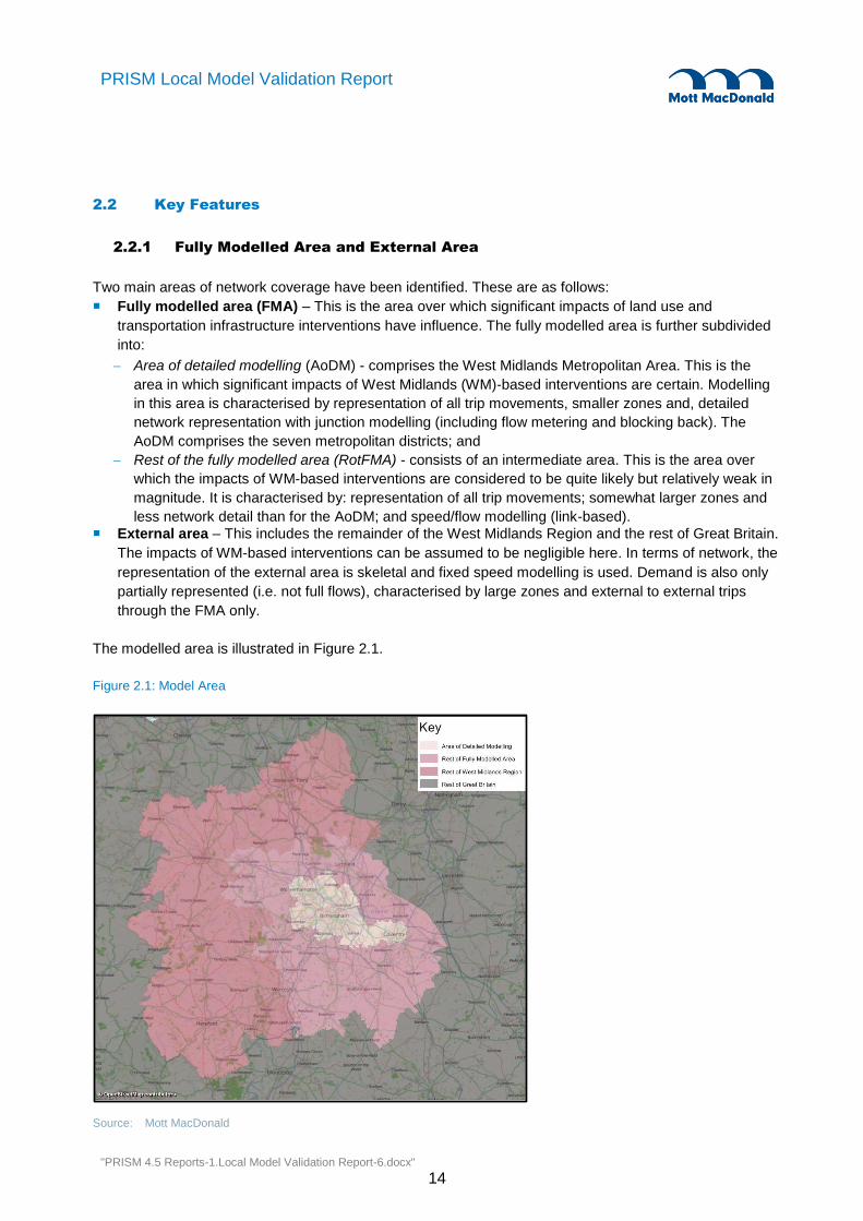
Two main areas of network coverage have been identified. These are as follows:
Fully modelled area (FMA) – This is the area over which significant impacts of land use and
transportation infrastructure interventions have influence. The fully modelled area is further subdivided
into:
Area of detailed modelling (AoDM) - comprises the West Midlands Metropolitan Area. This is the
area in which significant impacts of West Midlands (WM)-based interventions are certain. Modelling
in this area is characterised by representation of all trip movements, smaller zones and, detailed
network representation with junction modelling (including flow metering and blocking back). The
AoDM comprises the seven metropolitan districts; and
Rest of the fully modelled area (RotFMA) - consists of an intermediate area. This is the area over
which the impacts of WM-based interventions are considered to be quite likely but relatively weak in
magnitude. It is characterised by: representation of all trip movements; somewhat larger zones and
less network detail than for the AoDM; and speed/flow modelling (link-based).
External area – This includes the remainder of the West Midlands Region and the rest of Great Britain.
The impacts of WM-based interventions can be assumed to be negligible here. In terms of network, the
representation of the external area is skeletal and fixed speed modelling is used. Demand is also only
partially represented (i.e. not full flows), characterised by large zones and external to external trips
through the FMA only.
The modelled area is illustrated in Figure 2.1.
Figure 2.1: Model Area
Source: Mott MacDonald

"PRISM 4.5 Reports-1.Local Model Validation Report-6.docx"
15
PRISM Local Model Validation Report
2.2.2 Zoning System
2.2.2.1 Starting Point
The PRISM 2011 zoning system is largely based on the PRISM 2001 zoning system, which was originally
developed in 2002. As part of the PRISM Refresh, the zoning system was reviewed and updated. The
zoning system has also been informed by software and licensing limitations, details of which can be found
in section 2.2.2.2. The Centro public transport matrices and existing PRISM 2001 matrices have been used
in the matrix building and estimation process. The Centro PT and PRISM 2001 zoning systems have,
therefore, been used as the basis for the PRISM Refresh for reasons of consistency.
The zoning system consists of four distinct areas, with decreasing levels of detail:
The West Midlands county;
An intermediate area;
The rest of the West Midlands region; and
The rest of Great Britain.
The focus of PRISM is on modelling travel within the WM County, therefore the zoning has the most detail
in this area. However, it is recognised that a significant amount of travel (particularly commuting) within the
county originates from the hinterland around the county. Therefore an intermediate area consisting of a
band approximately 10-50 km in width around the county boundary is also modelled in some detail. Beyond
the intermediate area the next level of detail is the rest of the West Midlands region, followed by the rest of
Great Britain.
A number of issues were considered when developing the original zoning system in 2001:
How it affects the assignment model in terms of routing accuracy and the number of intra-zonal trips;
How it affects the accuracy of the demand model;
Obtaining demographic and land use data for calibrating the demand model;
Obtaining demographic and land use data for forecasting; and
Possible problems when building a base year trip matrix.
All the zone boundaries have been digitised in the MapInfo GIS package. The detailed PRISM zoning
system within the WM Metropolitan Area (county) is based on 1998 ward boundaries. Each ward is sub-
divided to form the model zones dependent on its size, land use characteristics, and population density of
the district in question.
2.2.2.2 Consultation
All members of the PRISM Management Group (PMG), comprising representatives from the seven Local
District Authorities, Highways Agency and Centro, were consulted on the redevelopment of the PRISM
2011 zoning system. The focus of this consultation was on the zoning system within the WM Metropolitan
Area; the AoDM. Through this consultation, the following objectives were considered in the PRISM 2011
zoning system:
A finer zoning system within local centres in the WM Metropolitan Area;
Compatibility between PRISM and Centro zones;
Compatibility between PRISM and Birmingham Lane Use and Transportation Study (BLUTS) zones;2
and
2 Zones are from the Birmingham City Centre model owned by Birmingham City Council.

"PRISM 4.5 Reports-1.Local Model Validation Report-6.docx"
16
PRISM Local Model Validation Report
Representation of existing and future land uses of strategic significance.
As a result of consultation, a number of minor revisions were made to the zoning system where possible,
however, any suggestions that would create an inconsistency in the zoning system across the WM
metropolitan districts, or that would exceed the limit on the total number of available zones were not
implemented. Any adjustments to the zoning system have been balanced with the necessity to stay within a
maximum number of zones (< approximately 995), due to Visum licensing constraints at the time and the
need to retain some zones for development areas that may be required in future applications. Another
consideration was the need to keep the number of zones to less than 1,000 as more would have an impact
on model run times.
The most significant update to the PRISM 2011 zoning system within the WM Metropolitan Area was the
further disaggregation of zones in local centres. For these areas of the zoning system, the Centro public
transport model zone structure was implemented to allow for disaggregation of city centres. The reason for
this was to improve the representation of routes and traffic flow and to provide a more detailed basis for
local modelling as well as to allow for the replacement of the PRISM 2006 PT model with an updated
version based on the Centro PT model. The Centro PT zones are a direct disaggregation of the highway
model zones which enabled the use of the former matrices.
In addition, a number of zones were split in order to better represent either existing or potential future land-
use changes within the WM Metropolitan Area. Further detail can be found in the Zoning Report.
2.2.2.3 PRISM Zoning System
A summary of the number of zones in each of the modelled areas is provided in Table 2.5., this was designed
for PRISM 4.1 and is unaltered for PRISM 4.5
Table 2.5: Number of PRISM zones by area
Modelled area Number of zones
WM metropolitan area 697
Intermediate area 254
Rest of the WM region 20
Rest of Great Britain 23
Total 994
Source: Mott MacDonald
2.2.3 Network Structure
2.2.3.1 Area of Detailed Modelling
The Area of Detailed Modelling comprises the West Midlands Metropolitan Area. This area is coded with a
high level of detail. All key minor and major roads are modelled. Key roads are considered to be those that
carry significant levels of traffic or provide means of access and egress to important developments within
the Area of Detailed Modelling. Capacity restraints are modelled through a combination of junction coding
and speed/flow relationships.

"PRISM 4.5 Reports-1.Local Model Validation Report-6.docx"
17
PRISM Local Model Validation Report
The area of the network around Birmingham International Airport and the NEC has been reviewed and
updated to include a greater level of network detail. This was done because the existing network coding
was not considered to include sufficient network detail.
2.2.3.2 Rest of the Fully Modelled Area
The Rest of the Fully Modelled Area comprises a buffer area around the Area of Detailed Modelling. The
network in the Rest of the Fully Modelled Area is represented in less detail, and for all roads capacity
restraint is modelled through the use of link-based speed/flow relationships only. Motorway junctions
considered to be of strategic importance that are situated within the Rest of the Fully Modelled area include
detailed junction coding.
2.2.3.3 External Area
The External Area represents the rest of Great Britain in a skeletal network. Junction coding is not used but
fixed “cruise” speeds are used for all roads.
2.2.4 Centroid Connectors
A zone centroid can be described as the centre of gravity, or trip attraction/generation, of a zone. During
the PRISM Refresh, zone centroids were calculated based on population within each zone. For zones with
a small or nil population, the zone centroids were calculated based on the centre of other activity within that
zone.
A connector is a special type of link that connects a zone centroid to a node in the road network; it
represents the point or points at which all traffic accesses the network. The following assumptions were
used when selecting the point at which to code a connector:
Connectors are coded realistically and, where possible, represent actual means of access to and egress
from the modelled network such as a car park for example;
Connectors do not cross barriers to movement such as rivers, railways, major roads and motorways;
Connectors do not connect directly onto a junction, unless a junction arm exists specifically for that
movement;
Connectors for neighbouring zones will not load on to the same node; and
The number of connectors per zone can be minimised, limiting them to one where possible.3
For PRISM 4.5, an extensive review of centroids and centroid connectors was carried out. This focussed
on areas with convergence noise or large static queues.
2.2.5 Time Periods
The PRISM Refresh base year highway assignment model represents an average weekday in 2011.
Highway assignment models have been developed to represent the average hour of the following time
periods:
AM; 0700-0930
IP; 0930-1530
PM; 1530-1900.
3 WebTAG Unit M3.1 (Sections 2.4.11 – 2.4.16)

"PRISM 4.5 Reports-1.Local Model Validation Report-6.docx"
18
PRISM Local Model Validation Report
Unlike previous versions of the PRISM model, it was decided not to explicitly model the OP (1900-0700)
time period in the model. This was due in part to the reduced amount of observed data collected in this time
period making validation more difficult, but also because it was felt any scheme being tested by the model
would have negligible benefits in the OP, and so modelling this was not required.
2.2.6 User Classes
Within PRISM, the modelled vehicle types are:
Car;
Light goods vehicles (LGV); and
Heavy goods vehicles (HGV).
Vehicle types are further split by journey purpose to allow for the variation in perceived travel cost between
different traveller types. A summary of PRISM user classes is shown in Table 2.6.
Table 2.6: PRISM user classes by vehicle type and journey purpose
PRISM user class Vehicle type Journey purpose
1 Car Business
2 Car Commuting and Other
3 LGV Employers Business
4 HGV Employers Business
Source: Mott MacDonald
Throughout all modelling work vehicles were represented in passenger car units (PCUs) based on the
conversion factors shown in Table 2.7 (as agreed with the PMG). WebTAG Unit M3.1 specifies different
PCU factors for HGVs by road type but it is not possible to do this within Visum, so a single factor was
assumed, this was to reflect HGVs on the strategic road network only.
Table 2.7: Passenger Car Unit conversion factors
Vehicle type Factor
Car/LGV 1
HGV 2.5
Bus 2.5
Source: Mott MacDonald
2.2.7 Delay Mechanisms
2.2.7.1 Implementing Capacity Restraint
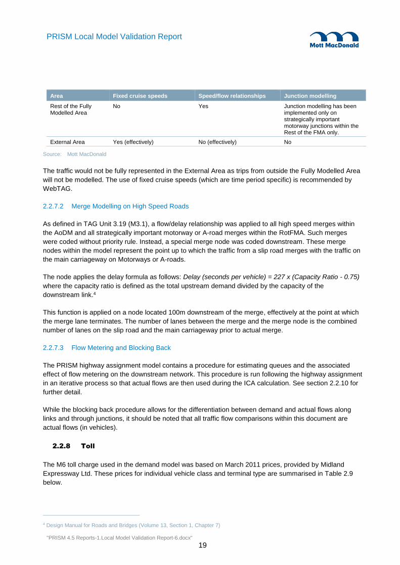
Table 2.8 provides a summary of how capacity restraint was implemented within the PRISM highway
networks. The table shows a summary of where junction modelling, speed/flow relationships and cruise
speeds were implemented prior to highway calibration.
Table 2.8: Capacity restraints within the PRISM Refresh highway network
Area Fixed cruise speeds Speed/flow relationships Junction modelling
Area of Detailed Modelling
No Yes Yes
"PRISM 4.5 Reports-1.Local Model Validation Report-6.docx"
19
PRISM Local Model Validation Report
Area Fixed cruise speeds Speed/flow relationships Junction modelling
Rest of the Fully Modelled Area
No Yes Junction modelling has been implemented only on strategically important motorway junctions within the Rest of the FMA only.
External Area Yes (effectively) No (effectively) No
Source: Mott MacDonald
The traffic would not be fully represented in the External Area as trips from outside the Fully Modelled Area
will not be modelled. The use of fixed cruise speeds (which are time period specific) is recommended by
WebTAG.
2.2.7.2 Merge Modelling on High Speed Roads
As defined in TAG Unit 3.19 (M3.1), a flow/delay relationship was applied to all high speed merges within
the AoDM and all strategically important motorway or A-road merges within the RotFMA. Such merges
were coded without priority rule. Instead, a special merge node was coded downstream. These merge
nodes within the model represent the point up to which the traffic from a slip road merges with the traffic on
the main carriageway on Motorways or A-roads.
The node applies the delay formula as follows: Delay (seconds per vehicle) = 227 x (Capacity Ratio - 0.75)
where the capacity ratio is defined as the total upstream demand divided by the capacity of the
downstream link.4
This function is applied on a node located 100m downstream of the merge, effectively at the point at which
the merge lane terminates. The number of lanes between the merge and the merge node is the combined
number of lanes on the slip road and the main carriageway prior to actual merge.
2.2.7.3 Flow Metering and Blocking Back
The PRISM highway assignment model contains a procedure for estimating queues and the associated
effect of flow metering on the downstream network. This procedure is run following the highway assignment
in an iterative process so that actual flows are then used during the ICA calculation. See section 2.2.10 for
further detail.
While the blocking back procedure allows for the differentiation between demand and actual flows along
links and through junctions, it should be noted that all traffic flow comparisons within this document are
actual flows (in vehicles).
2.2.8 Toll
The M6 toll charge used in the demand model was based on March 2011 prices, provided by Midland
Expressway Ltd. These prices for individual vehicle class and terminal type are summarised in Table 2.9
below.
4 Design Manual for Roads and Bridges (Volume 13, Section 1, Chapter 7)

"PRISM 4.5 Reports-1.Local Model Validation Report-6.docx"
20
PRISM Local Model Validation Report
Table 2.9: Actual cost of the toll in 2011
Car LGV HGV
Main Plaza £5.30 £10.60 £10.60
Local Plaza £4.00 £10.00 £10.00
Source: Midland Expressway Ltd
Within the route-choice element of the Visum highway assignment, a toll cost is modelled on the M6 toll to
reflect effects to the traffic distribution. The value that went into the model was calibrated to better reflect
the perceived cost to drivers so that a realistic distribution of flows was obtained. This was found to be 25%
of the true cost of the toll.
2.2.9 Generalised Cost Formulation
Generalised cost refers to both the monetary (i.e. fuel cost, vehicle operating cost) and non-monetary (i.e.
travelling time) costs of a journey. Generalised cost parameters are input as a series of values individual to
each user-class. Monetary values are input to Visum as pence per metre and non-monetary are input as
pence per second. These costs interact to affect route choice. If time is highly valued and distance is not
valued at all, the quickest journey will be chosen, no matter how long the distance. Similarly, if distance is
highly valued and time not at all, the shortest distance will be chosen.
Generalised cost values were calculated based on the vehicle operating costs, values of time and user
class splits as outlined within WebTAG. The resulting parameter values can be found in Table 2.10 and
Table 2.11. The Car Non-Work value is the averaged value of time for Car Commute and Car Other,
weighted by their matrix totals.
Table 2.10: Value of time (pence per minute)
Time period Car Work Car Non-Work LGV HGV
AM 54.60 13.40 21.83 36.38
IP 53.37 15.66 21.83 36.38
PM 52.59 13.57 21.83 36.38
Source: WebTAG
Table 2.11: Vehicle operating cost (pence per kilometre)
Time period Car Work Car Non-Work LGV HGV
AM 18.06 9.44 19.34 73.97
IP 18.36 9.58 19.56 75.38
PM 18.34 9.57 19.55 75.28
Source: WebTAG
2.2.9.1 Vehicle Operating Costs – Assumptions Used
In line with TAG Unit A1.3, paragraph 1.3.36, it was assumed that non-work users do not perceive non-fuel
costs.
In order to calculate fuel consumption it is necessary to state a network speed for each time period and for
each vehicle type. The average network speeds were calculated based on the network speeds in the

"PRISM 4.5 Reports-1.Local Model Validation Report-6.docx"
21
PRISM Local Model Validation Report
Highway model for individual vehicle types on all links within the boundary of the West Midlands
Metropolitan Area. The resulting speeds are shown in Table 2.12. Network speed data was based on
observed data from Trafficmaster, further information on this data is provided in Section 2.3.3.
Table 2.12: Assumed network speeds used in vehicle operating cost calculations
Time period Speed (km/h)
AM 27
IP 26
PM 26
Source: Mott MacDonald
2.2.9.2 Value of Time – Assumptions Used
Tag Unit M3.1 states that the value of time for HGVs in TAG Unit A1.3 relates to the driver’s time and does
not take into account the influence of owners on the routeing of these vehicles. For this reason, the value of
time for HGV can be, and has been, doubled.
2.2.10 Assignment Method
The assignment procedure used for the PRISM highway model is an interaction between a
subordinate/embedded assignment and a junction delay calculation, called Intersection Capacity Analysis
(ICA).
Key to the assignment process is the concept of volume delay functions (VDFs). These are similar to
traditional speed-flow curves, in that they can be used by a model to calculate the decrease in speed as
flow increases. In Visum it is the delay (travel time) on link/turn that is estimated, and the VDF describes
how this time increases as the traffic flow increases.
2.2.10.1 Overview, Assignment with ICA
The process can be view as in Figure 2.2, an embedded assignment is used to search for routes, this
produces network flows that are passed to the ICA module, then the ICA module estimates new VDFs taking
into account conflicting flows at turns. This process iterates until the entire system has reached equilibrium.

"PRISM 4.5 Reports-1.Local Model Validation Report-6.docx"
22
PRISM Local Model Validation Report
Figure 2.2: Assignment with ICA
Source: Mott MacDonald
2.2.10.2 Further detail on ICA assignments
This section gives further detailed information on the assignment process.
The assignment with ICA begins with an embedded assignment, which will be one of the three in built
equilibrium assignments (path-based, LUCE, or Lohse). In Visum, any variant of the equilibrium
assignment5 uses volume-delay functions for links and turns to represent the increasing delay with
increasing volume.
In urban network models, the turn VDFs are particularly important, since most delay (or variation in delay)
is generated by the junctions. The mathematical formulation of the assignment problem assumes, that the
delay which is calculated by the VDFs depends only on the volume and capacity of the individual network
link or turn. In reality whilst this holds approximately for links, it does not apply to turns. For example, the
capacity of a right turn from the minor arm of a priority junction would depend on the volumes on the
opposing turns from the major arms.
In order to account for this, the assignment procedure uses a node impedance calculation, called
Intersection Capacity Analysis (ICA) as well as the equilibrium assignment.
The ICA calculation requires that none of the flows are above capacity. The flows resulting from the
equilibrium assignment (hereafter referred to as demand flows) can go above link/turn capacity due to the
theoretical nature of assignment. To remedy this, a blocking back model is run within Visum to create what
we call actual flows – where no flow is greater than the capacity of turns.
5 assignment seeking to distribute demand according to Wardop’s principle of user equilibrium: “Every road user selects his/her route in such a way, that the impedance on all alternative routes is the same, and that switching to a different route would increase personal travel time”

"PRISM 4.5 Reports-1.Local Model Validation Report-6.docx"
23
PRISM Local Model Validation Report
This procedure reduces demand until no turns are above capacity and then feeds the excess demand back
into the model forming queues. As well as providing queues upstream from overcapacity junctions this also
produces an effect of reducing the flow after junctions as those vehicles are now represented in a queue,
this effect is known as flow metering. This process follows that described in detail in the paper “Modelling
Queues in Static Traffic Assignment”6
While the blocking back procedure allows for the differentiation between demand and actual flows along
links and through junctions, it should be noted that all traffic flow comparisons within this document are
actual flows (in vehicles) unless stated otherwise.
The full procedure is as follows:
An embedded equilibrium assignment is run to convergence. This assignment produces traffic flows on
links and turns. Blocking back has not yet been run, so these flows represent the demand flow;
The duality gap delta (d) statistic is relevant here, testing that the subordinate assignment has
reached Wardrop’s first principle of traffic equilibrium for the current delay curves being used.
The ICA calculation requires traffic flows to represent the actual flow, rather than demand, therefore, the
Blocking Back model is then launched. This procedure estimates queue lengths and wait time for
congested areas of the network. This procedure results in adjusted traffic flows which represent actual
flow;
Traffic flows are then “smoothed” by taking 70%7 of the flow from the current assignment iteration and
30% of the previous. This step is undertaken to aid convergence; and
These smoothed flows are then used in the ICA calculation, which produces new VDF parameters that
are fed into the next equilibrium assignment.
The %GAP statistic (if calculated) is an overall measure of convergence. Like delta, it tests whether the
current routes found by the subordinate assignment are sufficiently close to the minimum cost routes, but
using costs directly calculated from ICA rather than the estimated VDF curves. As such it is possible to have
a very good delta and a poor %GAP and so both should ideally be monitored.
2.2.10.3 Embedded Assignment
The PRISM highway models use an equilibrium assignment as the subordinate assignment procedure. This
procedure, distributes demand according to Wardrop’s first principle of traffic equilibrium:
“Under equilibrium conditions traffic arranges itself in congested networks in such a way that no individual trip
makers can reduce his path costs by switching routes”
The three equilibrium assignments available in Visum are:
1. Equilibrium (path-based)
Path based assignment, where equilibrium is reached on an OD basis.
2. Lohse
Developed by Professor Lohse, this models the “learning process” of road-users in the network, starting
with an ‘all or nothing’ assignment, drivers consecutively include information gained during their last journey
for the next route search.
3. LUCE (Local User-Cost Equilibrium)
6 “Modelling queues in static traffic assignment”, European Transport Conference (http://abstracts.aetransport.org/paper/index/id/2483/confid/12), Strasbourg, Bundschuh, M; Vortisch, P and van Vuren, T (2006)
7 This ratio was advised as standard by PTV, and subsequent testing by MM has confirmed it performs consistently well.

"PRISM 4.5 Reports-1.Local Model Validation Report-6.docx"
24
PRISM Local Model Validation Report
Similar to Origin-based assignment, this works on destination zones. The basic idea is, for any node a user
equilibrium is reached on all forward edges of the local route choice of drivers heading to a destination
zone.
We have tested the three assignment techniques, Lohse was found to take too long to converge to
acceptable levels, and the path-based assignment performed well and had been used in PRISM 4.1.
LUCE appeared able to achieve much tighter convergence within the embedded assignment however than
the other two options, and was recommended by PTV for use with ICA. It was slower than the path-based
assignment, but as run-times were still faster than PRISM 4.1 this was considered to be an acceptable
loss. For PRISM 4.5 LUCE was chosen as the embedded assignment.
2.2.10.4 A Brief note on Convergence
The two key statistics in convergence are the delta and the %GAP. These can be thought of as:
Delta: Testing the convergence of the embedded assignment
how close are the paths of that assignment to meeting Wardrop’s first principle of traffic equilibrium for the
specific link and turn VDFs
%GAP: Testing the overall convergence of assignment with ICA
how close are the paths of the most recent embedded assignment to meeting Wardrop’s first principle of
traffic equilibrium, when tested using the more accurate ICA delays
Visum calculates delta for the embedded assignment, but currently does not calculate %GAP. Other
statistics must hence be used to infer the convergence of the overall system.
2.2.11 Integration with the Public Transport assignment model
Public transport (PT) assignment models have also been developed during the PRISM Refresh. The
modelled time periods are as follows:
AM; 07:00-09:00
IP; 10:00-12:00
PM; 16:00-18:00.
The PT networks have been developed by Centro and Mott MacDonald and are linked to the highway
networks by a demand model developed by RAND Europe. The demand model has been built using an
extensive household travel survey, undertaken in 2011 and calculates forecasts to 2021 and 2031.
Direct linkages in the development of the highway and PT networks are:
A consistent zoning system within the AoDM; and
A bus pre-load - the number of services coded within the Public Transport networks have been used to
create a bus pre-load for the highway models. This pre-load is considered during the highway
assignment, whereby the bus pre-load multiplied by a PCU factor (2.5) is subtracted from the link and
turn capacity. Due to the scale of the network, only links/turns that have more than 10 services per hour
were given a bus pre-load (as agreed with PMG). This pre-load was also subtracted from the observed
traffic flow on relevant links during matrix estimation.

"PRISM 4.5 Reports-1.Local Model Validation Report-6.docx"
25
PRISM Local Model Validation Report
2.3 Calibration/Validation Data
2.3.1 Non-motorway
The volume of traffic count data required for calibration and validation during the PRISM Refresh prior
matrices was considerable. Guidance suggests that two-week ATC data should be used for model
development. However, collecting two-week ATC data and accompanying manual classified counts for the
number of sites for which data was required would have been a costly exercise, and not feasible within
given funding constraints. As a result, the following existing data sets have been interrogated to source
non-motorway and motorway traffic data.
2.3.1.1 Spectrum
Spectrum is a database of traffic count data collected within the West Midlands and maintained by Mott
MacDonald. Traffic count data for roads within the AoDM were extracted from Spectrum using the following
conditions:
Data is from an ATC;
The survey was undertaken between 2010 and 2012; and
The survey lasted one week or more.
Spectrum data was plotted on the highway network and used to derive screenlines and cordons. More
information regarding screenlines and cordons is given in section 2.6.4.
2.3.1.2 New Count Data
Screenlines and cordons have been checked for any data gaps on roads considered to be of strategic
importance. As a result, 23 new one-week ATCs were undertaken within the AoDM in October and
November 2012.
2.3.1.3 Ad hoc Data
Additional traffic count data was provided by Sandwell MBC.
2.3.1.4 Roadside Interviews
ATC data collected at the time of the PRISM Refresh RSIs were used in matrix estimation.
There are two sources of RSI traffic count data:
Coventry RSIs conducted in 2009; and
PRISM Refresh RSIs conducted between 2010 and 2011.
A list and map of the sites used is provided in Appendix A.
2.3.1.5 Factoring
The non-motorway traffic count data used within the PRISM Refresh was collected between 2010 and
2012. In order to account for variability in traffic flow over and between different years, a series of factors
have been applied to all non-motorway traffic count data in order to account for known variability in traffic
volume over time.

"PRISM 4.5 Reports-1.Local Model Validation Report-6.docx"
26
PRISM Local Model Validation Report
A series of factors have been derived for this purpose:
Factors to account for the known seasonal variation in traffic throughout a year; and
Factors to account for average change in traffic between years.
The factors were calculated from the ATC data 2008-2012 from Spectrum. All traffic counts had a seasonal
factor applied depending on the date the count was undertaken and an annual factor applied depending on
the year the count was collected. The factors applied to the traffic count data can be found in Appendix B.
2.3.2 Motorway
The HE Traffic Information System (HATRIS) contains the Traffic Flow Data System (TRADS), a database
maintained by the Highway Agency that contains information on traffic flows at sites on the strategic road
network. Traffic count data was extracted from TRADS for motorway sites and processed as follows:
1. 2011 yearly tabular data for each site was downloaded, providing a traffic count for each hour of the year;
2. Annual average Monday-Friday traffic volumes for each of the modelled time periods, for each site, were
calculated;
3. The monthly classified counts for the same sites for October 2011 were downloaded;
4. Using the monthly classified data, the percentage HGVs (>6.6m in length) for each modelled time period,
for each site was calculated; and
5. The percentage HGVs was applied to the average traffic volume to derive light and heavy traffic counts.
The traffic volume was calculated on annual data from 2011, as such no further factoring was required.
2.3.3 Journey Times
Trafficmaster (TM) historical journey time data was used to extract observed journey time data for routes
within the AoDM.
TM is congestion data produced by Trafficmaster Plc and provided to local authorities by the Department
for Transport. The data is collected by placing GPS trackers in fleet vehicles and recording journeys. This
data is then mapped onto the OS ITN. With the data matched to road links, it is possible to calculate
average observed speeds on links.
Due to the road network changing, the Ordnance Survey Integrated Transport Network (OS ITN) is updated
annually. For this reason TM use a new version of ITN each year. As the GPS data is also date and time
stamped it is possible to filter the data by specific day types, e.g. term time etc. and by time period.
For the PRISM Refresh, data from the academic year 2010/11 was used and was filtered by term time only
and for the four time periods as defined below:
AM; 0700 – 0930
IP; 0930 – 1530
PM; 1530 – 1900
OP; 1900 – 0700.
Data for the academic year was selected to eliminate any variations in the traffic pattern due to the school
holidays.

"PRISM 4.5 Reports-1.Local Model Validation Report-6.docx"
27
PRISM Local Model Validation Report
2.4 Network
Rather than begin building the networks from scratch, the network from the previous version of PRISM was
used as a starting point. For PRISM 4.5 the validated networks from PRISM 4.1 were used as the starting
point. In turn PRISM 4.1 used the PRISM 3.2 (2006 base year) network as a starting point.
2.4.1 Data Sources
The existing PRISM 2006 base year network was used as the basis for the PRISM 2011 highway network.
GIS data sources were also used to update highway network elements. The Ordnance Survey (OS) Master
Map® Integrated Transport Network (ITN) dated August 2011 was used to inform the coding of updated
junction layouts. The ITN was layered underneath the PRISM highway network within Visum. This allowed
for junctions and links to be coded accurately. Data from NAVTEQ Maps data (Q4, 2011) was used to code
speed limits and to check the number of lanes on links within the Fully Modelled Area. These two sources
of GIS data were supplemented by aerial photography.
2.4.2 Junctions
The effect of junctions is a key determinant in route choice within the AoDM and strategically important
motorway junctions within the RotFMA. The highway network contains approximately 11,000 nodes, 7,000
of which are within the AoDM. Of these, approximately 3,500 are priority nodes, 850 signalised and 600
roundabouts. The remaining nodes are uncontrolled. All junctions within the AoDM are modelled using ICA.
Junctions within the AoDM are coded in detail to include the following:
Control type (method for controlling vehicle movements at a junction, if any);
Number of junction approaches;
Junction operation in terms of lane allocation;
Conflicts between vehicle movements; and
Signal timings.
The Intersection Capacity Analysis (ICA) module within Visum has been used in conjunction with an
equilibrium assignment to model junction delay within the AoDM. In order to correctly model a junction
using ICA, it is necessary to specify junction geometry, including the number of lanes per approach, the
permissible turns per lane, and the number of flared lanes.
For the majority of junctions, aerial photography from Google Maps has been used to obtain information on
junction layout and operation. Where aerial imagery may have been out of date (the date stamp of the
image was earlier than 2010/2011), junction details were obtained by using site layout drawings,
undertaking site visits or, in a few cases, liaising with Local Authorities.
2.4.2.1 Priority Junctions
In order to model priority junctions using the ICA function within Visum, the following data is required:
The number of lanes for all junction approaches;
The priority arrangement, including major flows; and
The lane arrangement, including permissible turns per lane.
"PRISM 4.5 Reports-1.Local Model Validation Report-6.docx"
28
PRISM Local Model Validation Report
Within Visum, the most important attribute for priority nodes is the major flow, i.e. the allocation of priority at
the node. The major flow orders all turning movements through a node into a hierarchy, whereby delay is
assigned to the minor movements.
2.4.2.2 Roundabout Junctions
The approach used to code a roundabout within the PRISM networks is dependent upon the type and
operation of the roundabout:
Signalised roundabouts are coded as a series of one-way links and signal controlled nodes. There are
around 50 signalised roundabouts. This is because it is not possible to code a signalised roundabout as
a single node within Visum. The coordination of signals is not represented in the model;
Grade separated roundabouts are also coded as a series of one-way links and priority controlled or
signalised nodes. There are approximately 60 grade separated roundabouts. This is because the layout
of these junctions lends itself to becoming signalised in the future, and this method of coding allows link
lengths of the gyratory to be included within route choice; and
Other roundabouts are coded as a single node using the roundabout control type. There are around 600
roundabouts of this type.
For roundabouts coded as a single node, delay is calculated using the Kimber/TRL method, which requires
that, for each roundabout approach, detailed geometry measurements are input, such as entry width, flare
length and approach half width. These are the same measurements that would be required for other
roundabout junction modelling software, such as ARCADY. Due to the size of the PRISM 2011 highway
network and the high cost associated with collecting this data for each roundabout, a template approach
was developed for all roundabout junction approaches, whereby each approach was given default values,
some of which were adjusted during network calibration.
2.4.2.3 Signalised Junctions
There are approximately 900 signalised junctions modelled in PRISM 2011 within the AoDM. In order to
model signalised junctions using the ICA function within Visum, the following data is required:
Number of lanes for all junction approaches;
Lane arrangement; and
Signal staging and timing data.
Signal specifications have been provided by the seven metropolitan authorities for the majority of signalised
junctions within the AoDM. Each signalised node has been coded with basic staging arrangements as
provided in the signal specification.
2.4.2.4 Observed Signal Timings
Traffic signal timings were collected for each signalised junction within the PRISM model through liaison
with the relevant local highway authority. The councils at Birmingham, Coventry, Sandwell, Solihull and
Wolverhampton each have dedicated Urban Traffic Control (UTC) centres. Traffic signals in Walsall and
Dudley are operated through Wolverhampton’s control centre.
Wherever possible, the timings were based on recorded data. This was possible wherever the junction was
connected to the local Urban Traffic Control (UTC) centre or where the junction operated on MOVA (Micro-
processor Optimised Vehicle Actuation) control. The signal timings collected were stage based rather than

"PRISM 4.5 Reports-1.Local Model Validation Report-6.docx"
29
PRISM Local Model Validation Report
phased based, giving stage and inter-stage times. The inter-stage times were calculated from the traffic
signal controller specification for each junction.
For junctions that did not have recorded signal timings available, or where the recorded data was clearly
incorrect, the stage times were calculated using the maximum green times in the controller specification.
These green times are the maximum time that the controller will allow the signal to be on green when
operating under VA (Vehicle Actuation) control. Whilst these are unlikely to be the actual signal times, they
are likely to give reasonably realistic green splits between stages. In other words, the green time is divided
proportionally between stages based on the amount of traffic demand for each stage.
Diagrams have been produced showing which signals are using observed signal timings, and which are
using estimated timings, these are included in the appendix for each district, and an overall plot is sown
below.
Figure 2.3: PRISM Signals
Source: Mott MacDonald
2.4.3 Links
Table 2.13 summarises the link data requirements for the highways networks.
Table 2.13: Link data requirements
Data Source/description
Link type Link types have been derived and applied in line with TAG Unit M3.1. Further detail is provided in Section 2.4.3.1.
Capacity Link capacities have been calculated in line with TAG Unit M3.1. Further detail is provided in Section 2.4.3.1.

"PRISM 4.5 Reports-1.Local Model Validation Report-6.docx"
30
PRISM Local Model Validation Report
Data Source/description
Speed/flow relationship
Speed/flow relationships have been calculated based on TAG Unit M3.1.
Length ITN has been layered onto the highway network within Visum, allowing nodes to be placed accurately and links to be shaped accordingly. Link lengths have been set to the link polygon length.
Number of effective lanes
The number of lanes on a link has been coded as the number of lanes that are available to highway traffic under normal operation. For example, if a road has two lanes but the inside lane is used for on-street parking; the link would be coded with one lane within Visum as this best reflects the operation of this link in reality. Similarly, if a road is two lanes wide but one is a bus-only lane, the link would be coded with one lane in Visum. The bus only lane will not be coded as a separate link, because public transport trips will not be assigned onto the highway network. Bus flows have been taken into account in the assignment as a pre-load, except where bus flows are on a bus-only link or lane.
Direction (one-way or two-way)
One-way links have been coded based on ITN and aerial photography.
Vehicular restrictions
Vehicular restrictions relating to weight restrictions have been coded based on ITN data. Bus only links have been banned to private transport.
Speed limit Speed limit data has been sourced from NAVTEQ. This data has been used as it is the best source available. The inclusion of speed limit data allows for sense checks against cruise speed data to be made.
Cruise speed The calculation of this value is dependent on a number of conditions as discussed in Section 2.4.3.3
Source: Mott MacDonald
2.4.3.1 Link Types
Table 2.14 summarises link types within the highway networks.
Table 2.14: Link types
Road class Description Speed limit Capacity (PCU/lane)
1 Rural single carriageway 50mph - 60mph 1330
2 Rural all-purpose dual 2-lane carriageway 50mph - 70mph 2100
3 Rural all-purpose dual 3 or more lane carriageway 50mph - 70mph 2100
4 Motorway, dual 2-lanes 50mph - 70mph 2330
5 Motorway, dual 3-lanes 50mph - 70mph 2330
6 Motorway, dual 4 or more lanes 50mph - 70mph 2330
7 Managed (Smart) Motorway, dual 4 lanes 60mph during controlled periods
2330
8 Small town 30 to 40mph 1340
9 Suburban single carriageway 30 to 50mph 1680
10 Suburban dual carriageway 30 to 50mph 3540
11 Urban 20 to 30mph 800
12 External motorway 70mph 2330
13 External non-motorway 30 to 50mph 2100
Source: Mott MacDonald
2.4.3.2 Speed/Flow Relationships
Speed/flow relationships have been defined for all link types in Table 2.14. In the External area, where
Table 2.8 stated that fixed speeds have been used, very flat curves have been implemented to proxy a
fixed speed. Flat curves have been used (rather than a fixed speed) to aid assignment convergence. This
was also the case for roundabout links in the urban area.

"PRISM 4.5 Reports-1.Local Model Validation Report-6.docx"
31
PRISM Local Model Validation Report
The parameters used in the speed/flow curves are based on those provided by HE TAME which in turn are
based on those in COBA. The curves provided by HE TAME include over-capacity ‘tails’ which have not
been replicated in PRISM due to the use of the Visum blocking back model. Figure 2.4 provides an
example for a two-lane dual carriageway link type where the PRISM (Visum) curve has been fitted to the
HE TAME curve for flows below capacity. For over-capacity conditions in PRISM the blocking back model
will kick in.
Link capacities are coded in PCUs in PRISM, using the following PCU factors:
Cars: 1
LGVs: 1
HGVs: 2.5.
As described in Section 2.2.11, bus flows have been modelled as a pre-load, a separate PCU factor of 2.5
has been applied for these.
Figure 2.4: Speed-flow curve development for two-lane dual carriageways
Source: Mott MacDonald
It is suggested in TAG Unit M3.1 that the use of separate speed/flow relationships for light and heavy
vehicles is preferred for rural and suburban speed/flow curves because this could provide more accurate
estimates of changes in vehicle operating costs and travel times. It is not practicable to adopt this approach
in PRISM as Visum does not have the necessary functionality inbuilt. However, a maximum speed for
HGVs has been applied in Visum and this was implemented as follows (based on the Highway Code,
2007):
30mph in built-up areas (all 30 mph roads);
40mph on single carriageways;
0.00
20.00
40.00
60.00
80.00
100.00
120.00
km
/h
PCU Flow (capacity is 4200)
TAME Speed (km/h)
VISUM Speed (km/hr)

"PRISM 4.5 Reports-1.Local Model Validation Report-6.docx"
32
PRISM Local Model Validation Report
50mph on dual carriageways; and
56mph on motorways.
Maximum speed has also been applied to LGVs as follows (based on the Highway Code, 2007):
50mph on single carriageways; and
60mph on dual carriageways.
In all other instances (mainly where the maximum speeds defined for LGVs or HGVs are higher than the
speed limits defined for a particular link type, Table 2.14) same speed limits are applied to all vehicle types.
2.4.3.3 Cruise Speeds
Cruise speed can be defined as “the mid-link speed, separate from any junction delay, during the time
period modelled” (TAG Unit M3.1.
Guidance states that one way of deriving mean cruise speeds is to establish a relationship between
attributes of a link, such as road type, speed limit, activity levels and cruise speeds to estimate a mean
cruise speed for each link in the network TAG Unit M3.1
Cruise speeds have been implemented as the ‘free-flow’ speed for use in conjunction with the link speed-
flow curves and junction modelling.
2.4.3.4 Cruise Speeds – Area of Detailed Modelling
Speed data captured by automatic traffic counters (ATC) in mid-block sections of road, where speeds
would be less influenced by the presence of junctions was interrogated. The process adopted was as
follows:
Match ATC speeds with the 30 mph 1 and 2-lane roads in the PRISM central and non-central area;
Derive average speeds for each of those links from the speed data by time period; and
Calculate overall average speed for 30 mph 1 and 2-lane link types in central and non-central area by
time period.
Based on the above, a single cruise speed of 18mph was assumed for all urban roads in the AM/IP/PM
time periods.
2.4.3.5 Cruise Speeds – External Area
The Highways Agency provided observed speeds for a selection of motorway and non-motorway links for
weekdays in 2011 in the External Area. This data has been used to calculate separate average speeds for
motorway and non-motorway links. Table 2.15 lists the calculated average speeds.
Table 2.15: Cruise speeds – external links
Time period Motorway Non-Motorway
AM 67 48
IP 67 50
PM 67 49
Source: Calculated from observed speed data provided by the Highways Agency

"PRISM 4.5 Reports-1.Local Model Validation Report-6.docx"
33
PRISM Local Model Validation Report
In agreement with the PMG, the final cruise speeds for external links were assumed to be:
Motorway – 67mph for all time periods; and
Non-motorway – 50mph for all time periods.
2.5 Trip Matrix
2.5.1 Travel Demand Data
A substantial amount of data for the highway matrix build was collected during the period 2009-2011. This
dataset consists of:
Roadside interview survey (RSI) data collected at 90 sites;
Manual classified counts (MCCs) at the 90 RSI sites;
Automatic traffic counts (ATCs) for the RSI sites and for other additional sites across the West
Midlands Metropolitan Area;
Car park surveys for 53 urban sites; and
GPS data (Trafficmaster and INRIX).
In addition, 2011 Census journey to work matrices alongside synthetic trip matrices from PRISM 4.1 were
used in the matrix building process.
2.5.1.1 RSI Data
RSI records form the major source of data for the PRISM Refresh matrix build. The survey data was a mix
of face-to-face interviews and self-completion postcards covering travel information over the period 0700-
1900. The roadside interviews were carried out only in one direction and did not cover the off-peak period.
An off-peak model was not built for PRISM, as previously mentioned in section 2.2.5. The 90 RSI sites
consisted of:
76 sites that captured movements into/from Birmingham, Wolverhampton, Walsall, Dudley, Sandwell and
Solihull collected by Mott MacDonald; and
14 sites within and around Coventry provided to Mott MacDonald by Coventry City Council, which were
collected for the purpose of developing a local model in Coventry.

"PRISM 4.5 Reports-1.Local Model Validation Report-6.docx"
34
PRISM Local Model Validation Report
The location of the sites can be seen in Figure 2.5.
Figure 2.5: Location of RSI interviews
Source: Mott MacDonald
Further detail can be found in PRISM Surveys 2011: Roadside Interviews.
2.5.1.2 MCC Data
MCC data was collected over the 12 hour survey period for each of the 90 RSI sites for both interviewed
and non-interviewed directions.
2.5.1.3 ATC Data
ATC data was collected for each of the 90 RSI sites for both interviewed and non-interviewed directions.
ATC data was collected over a two week period.
2.5.1.4 Car Park Surveys
Car park data was collected in the form of self-completion postcards for off-street car parks only.
Locations of the 53 surveyed car parks are given in Table 2.16.
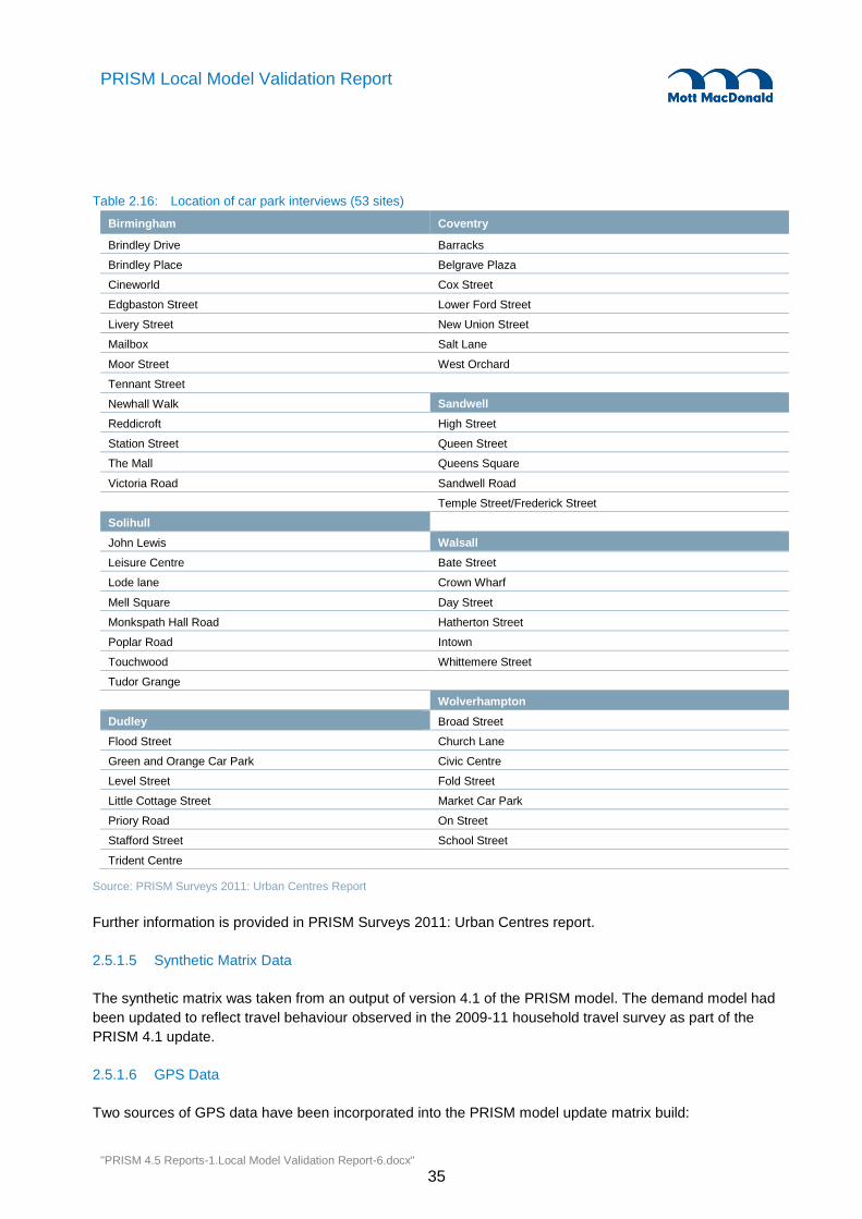
"PRISM 4.5 Reports-1.Local Model Validation Report-6.docx"
35
PRISM Local Model Validation Report
Table 2.16: Location of car park interviews (53 sites)
Birmingham Coventry
Brindley Drive Barracks
Brindley Place Belgrave Plaza
Cineworld Cox Street
Edgbaston Street Lower Ford Street
Livery Street New Union Street
Mailbox Salt Lane
Moor Street West Orchard
Tennant Street
Newhall Walk Sandwell
Reddicroft High Street
Station Street Queen Street
The Mall Queens Square
Victoria Road Sandwell Road
Temple Street/Frederick Street
Solihull
John Lewis Walsall
Leisure Centre Bate Street
Lode lane Crown Wharf
Mell Square Day Street
Monkspath Hall Road Hatherton Street
Poplar Road Intown
Touchwood Whittemere Street
Tudor Grange
Wolverhampton
Dudley Broad Street
Flood Street Church Lane
Green and Orange Car Park Civic Centre
Level Street Fold Street
Little Cottage Street Market Car Park
Priory Road On Street
Stafford Street School Street
Trident Centre
Source: PRISM Surveys 2011: Urban Centres Report
Further information is provided in PRISM Surveys 2011: Urban Centres report.
2.5.1.5 Synthetic Matrix Data
The synthetic matrix was taken from an output of version 4.1 of the PRISM model. The demand model had
been updated to reflect travel behaviour observed in the 2009-11 household travel survey as part of the
PRISM 4.1 update.
2.5.1.6 GPS Data
Two sources of GPS data have been incorporated into the PRISM model update matrix build:

"PRISM 4.5 Reports-1.Local Model Validation Report-6.docx"
36
PRISM Local Model Validation Report
Trafficmaster - provided by the Department for Transport (DfT) for use in the PRISM model update.
The data covered a 12 month period (August 2010 - August 2011) and originates from vehicles
belonging to Trafficmaster customers who are primarily high mileage vehicle drivers and company car
drivers and HGVs.
INRIX – due to the low OD coverage in the Trafficmaster HGV matrices, INRIX data served as a
primary source of heavy goods vehicle data. Due to costing implications the data used in this project is
restricted to movements that went through (or had an origin or destination) within a 30 mile box with its
centre in Birmingham over the 7 month period April 2011 to October 2011. Vehicle journeys that had an
origin outside of this box were recorded as having an origin zone on the box boundary (at the point of
which the vehicles journey crosses the bounding box), likewise for destination zones. Because of this
trip-length information is not directly comparable with other data sources, as the longer journeys are cut
short at this boundary, however it does mean that trip-routeing through the modelled area is potentially
more accurate than if the longest trips had been assigned to the coarser external zones.
2.5.2 Partial Trip Matrices from Surveys
The observed matrices are comprised of RSI, car park and GPS data. All data used in the matrix build has
been converted to the common PRISM origin-destination format prior to being developed into the trip
matrices.
2.5.2.1 RSI Matrices
The RSI matrices were produced from the expanded RSI records. Prior to the expansion, RSI records were
processed into a common format and inconsistent and illogical records have been eliminated from the data
(including missing or incomplete data, illogical origins and/or destinations and outbound and/or return travel
times). These represent around 6% of all records.
The following steps were undertaken to convert the RSI data to a single format:
Trip purpose mapping from trip purpose at origin or destination and conversion to the trip purposes
used in the 2011 PRISM model, including: commuting, business, education and other;
Vehicle type identification and allocation to the vehicle type categories used in PRISM;
Establishing time of inbound and outbound travel. As the roadside interviews were conducted only in
one direction, the interview time was used as the time of travel for the outbound trip. The reverse trip
was either stated on the interview form or estimated from trip purpose analyses;
Allocation of time periods and time slots to interview records. Trips were assigned to AM, IP, PM or OP.
Within these time periods, records were also assigned to a 30 minute time slot that was used during the
expansion of the interview records;
Allocation of zone numbers to the interview records. Postcodes were captured on the interview forms.
This stage mapped postcodes to Ordnance Survey Grid Reference (OSGR) and then model zones for
each record; and
Expansion of interview records to manual classified counts. This is the basic record expansion stage.
Additional adjustments then follow:
− Adjustments of the base expansion factors to site ATC counts;
− Adjustment of expansion factors to average weekday ATCs;
− Adjustment to common year/common month; and
− Adjustments for postcard interview records to address response bias.

"PRISM 4.5 Reports-1.Local Model Validation Report-6.docx"
37
PRISM Local Model Validation Report
The MCC expansion factor was derived as follows:
𝐸𝑥𝑝𝑎𝑛𝑠𝑖𝑜𝑛 𝐹𝑎𝑐𝑡𝑜𝑟 (𝑠, 𝑣, 𝑡) =𝑀𝐶𝐶(𝑠,𝑣,𝑡)
𝑅 (𝑠,𝑣,𝑡);
where:
MCC(s, v, t) – relevant manual classified count in 30 minute interval; and
R(s, v, t) – sum of all interview records for a particular site (s), 30 minute time slot and vehicle type
(v).
The expansion factor was then aligned to the corresponding ATCs. Since ATC is a more accurate count
but lack detailed vehicle classification, the adjustment factor was calculated as:
𝐴𝑇𝐶 𝐹𝑎𝑐𝑡𝑜𝑟 (𝑠, 𝑣, 𝑡) =𝐴𝑇𝐶 (𝑠,𝑣,𝑡)
𝑀𝐶𝐶 (𝑆,𝑣,𝑡);
where:
𝑡 – hourly time slot.
The factors were adjusted to average weekday ATC totals. In the data used for this work, ATCs were
generally available for a period of two weeks for each survey site. The initial expansion factors were therefore
adjusted by the average weekday factor calculated as:
𝑊𝑒𝑒𝑘𝑑𝑎𝑦 𝐹𝑎𝑐𝑡𝑜𝑟(𝑡) =𝐴𝑇𝐶(𝑎𝑣𝑒𝑟𝑎𝑔𝑒 𝑤𝑒𝑒𝑘𝑑𝑎𝑦,𝑡)
𝐴𝑇𝐶(𝑖𝑛𝑡𝑒𝑟𝑣𝑖𝑒𝑤 𝑑𝑎𝑦,𝑡).
Additional adjustment was to convert the data to a common year of 2011. Coventry data was collected in
2008 and 2009. This was adjusted to 2011 using the relative average annual weekday ATCs from
permanent sites:
𝑌𝑒𝑎𝑟 𝐹𝑎𝑐𝑡𝑜𝑟 =𝐴𝑣𝑒𝑟𝑎𝑔𝑒 𝑤𝑒𝑒𝑘𝑑𝑎𝑦 𝐴𝑇𝐶(𝑌𝑒𝑎𝑟)
𝐴𝑣𝑒𝑟𝑎𝑔𝑒 𝑤𝑒𝑒𝑘𝑑𝑎𝑦 𝐴𝑇𝐶(2011).
Final step was to adjust postcard interview records to address response bias. Postcard data is usually
skewed towards some travel purposes. The purpose of this adjustment was to bring postcard responses in
line with RSI face-to-face interviews. Data availability did not allow this to be done by site. So for all sites,
taken together and for purpose p, the postcard factor was determined by:
𝑃𝑜𝑠𝑡𝑐𝑎𝑟𝑑 𝐹𝑎𝑐𝑡𝑜𝑟 =𝑃𝑜𝑠𝑡𝑐𝑎𝑟𝑑 𝑡𝑜𝑡𝑎𝑙 (𝑝)
𝑅𝑆𝐼 𝑡𝑜𝑡𝑎𝑙 (𝑝).
The PRISM model area was partitioned into 10 sectors in order to aid matrix building and analysis of traffic
movements throughout the AoDM. Sectors 1-5 represent the AoDM (Figure 2.6) while sectors 6-10
represent the RotFMA and external area where modelling detail is not crucial (Figure 2.7).

"PRISM 4.5 Reports-1.Local Model Validation Report-6.docx"
38
PRISM Local Model Validation Report
Figure 2.6: Sectors within West Midlands
Source: Mott MacDonald
Figure 2.7: Intermediate and external sector coverage
Source: Mott MacDonald

"PRISM 4.5 Reports-1.Local Model Validation Report-6.docx"
39
PRISM Local Model Validation Report
The ERICA software was used to develop RSI matrices. The screenline segments were defined in line with
the requirements of the software. ERICA matrix build screenlines connect RSI sites and were defined to
capture fully observed movements.
RSI data was assigned to cordons and screenline segments before the matrices were produced. Since RSI
data did not capture all of the movements through the cordons, additional data for omitted roads that
looked significant was collected from the following sources:
1500 survey, a set of ATCs that are collected periodically across West Midlands;
Spectrum, a set of ATCs that has the 1500 survey as a subset; and
New traffic counts. These were counts specifically requested where the 1500 survey and Spectrum
counts did not cover a particular road.
The counts on these additional roads were used to adjust count totals at adjacent RSI sites before they
were used in the matrix build. The assumption was that trips passing through that screenline would follow
the same pattern as those at the RSI site. This way, more accurate levels of traffic were recorded across
cordons and screenlines.
This then formed the input to ERICA which held the full set-up files for combining the site data into time
periods and purposes as well as removing any double counting in the matrix build process and also dealing
with movements that may cross a cordon more than once. Double counting occurs where observed
movements for the same OD pair are observed and expanded at different cordons of RSI sites. A route
could potentially cross a screenline more than once with the same observed movement counted and
expanded at two sites for the same trip.
2.5.2.2 Car Park Matrices
The car park records used in the development of car park matrices were modified and expanded in the
following way:
The time periods that were derived for the RSI records were applied in a similar way to the car park
records. The length of stay and return time provided an estimate of the time of travel for inbound and
outbound trips;
Car park postcodes were considered to be the final destinations for inbound trips (and the origins for
outbound trips);
Expansion factors were applied to account for unobserved arrival flow at off-street car parks; and
Expansion factors were applied to account for unobserved on-street and PNR car parks.
Since information regarding on-street and PNR car parks was unavailable, comparison of an assignment of
the synthetic matrix with the un-expanded car park matrix was used to create expansion factors that took
into account off-street car parks.
2.5.2.3 GPS Matrix Build
The DfT provided Trafficmaster (TM) data in the form of individual trip records in the TM zoning system.
The TM data was aggregated into total annual weekday trips by TM vehicle types and TM time periods.
The TM data for car is not split by trip purpose, as opposed to PRISM. It should also be noted, that there
was a 30 minute mismatch between TM and PRISM time period boundaries for Inter Peak and PM Peak. It
was decided to not produce factors to remove this inconsistency explicitly as the total volume was then
factored based on RSI totals later in the process, by definition this implicitly corrected the time periods

"PRISM 4.5 Reports-1.Local Model Validation Report-6.docx"
40
PRISM Local Model Validation Report
mismatch (to the same extent as factoring could have done). Further details on the volume scaling can be
found below.
In order to develop GPS origin-destination matrices, the following adjustments were made to the TM data:
Conversion to the PRISM zoning system;
Creation of car trip purpose splits; and
Use of INRIX data to supplement the scarce HGV data in the TM matrices.
The TM zoning system was provided with MapInfo files that allowed a correspondence with the PRISM
zonings system to be made. This was done by overlapping the two zoning systems and applying the
following simple rules:
If a TM zone was more than 90% in a PRISM zone, then all trips were assigned to that PRISM zone.
Otherwise, the TM zone was split between corresponding PRISM zones according to area of overlap; and
If a TM zone is larger than a PRISM zone, then the TM zone was split to PRISM zones according to area
proportions in the overlaps.
This process yielded matrices in the 994 zone system that the PRISM model uses.
The data did not have trip purpose information as TM does not hold information on journey purposes for its
customers. Therefore the TM car matrices created from TM records were broken down into business,
commute and other trip purposes using synthetic data.
The TM data has been treated as a random sample of car trips, so to remove any sampling bias the trip
length distribution derived from the National Travel Survey (NTS) data has been used. The TM purpose
split was calculated based on the ratio of business, commute and other trips per OD as calculated by the
PRISM demand model.
It was agreed with the PRISM Management Group that due to the differences between INRIX and
Trafficmaster data for HGVs and owing to their different sources, adding the two data sets together and
then factoring the totals was more appropriate than merging.
The following matrices were generated from the TM data for the four modelled time periods:
Car business;
Car commuting;
Car other;
LGV; and
HGV.
2.5.3 Census 2011 Journey to Work Matrices
The Census data provides records aggregated to MSOA zones, these records contain home address and
usual place of work. Using trip rate information derived from the West Midlands Household Interviews this
information was converted into an all-day tour matrix. This was further disaggregated into PRISM zones
and into time periods using local data.
This information was used to supplement the commute-purpose trips in the highway matrix build.

"PRISM 4.5 Reports-1.Local Model Validation Report-6.docx"
41
PRISM Local Model Validation Report
2.5.4 Trip Synthesis
The synthetic matrix was taken from version 4.1 of the PRISM model. The demand model had been
updated to reflect travel behaviour observed in the 2009-11 household travel survey, and land use
assumptions that fed the demand model were updated with data available from the 2011 Census including
recession impacts and recently updated datasets such as educational enrolment data and employment
data aggregated from the Inter-Departmental Business Register (IDBR). The resulting matrices were used
as synthetic matrices for the full build.
Since the 2011 costs from Prism 4.5 highway and PT networks were not available at the time of the matrix
build, travel costs used in the estimation of demand were based on the PRISM 4.1 models.
2.5.5 Merging Data
The matrix merging process was carried out with a series of python programs specifically developed for this
purpose.
2.5.5.1 Matrix Scaling
The RSI matrix represented the major directly observed dataset in the development of the prior matrices
and was used as a benchmark for the rest of the matrices used in the merging process. Since the size
and/or the shape of the other matrices did not correspond, additional adjustments had to be applied before
they could be used further in the merging process.
For each non-RSI matrix, a single factor was produced to ensure the matrices were of comparable size to
the RSI observed total. This calculation was carried out by comparing the volume of trips in the RSI matrix
with the volume in the target matrix for RSI-observable movements only. i.e. only the volume from the
sector to sector movements that could have been observed by an RSI survey. These movements have
been highlighted in the figure below.
Figure 2.8: RSI observable movements
Source: Mott MacDonald

"PRISM 4.5 Reports-1.Local Model Validation Report-6.docx"
42
PRISM Local Model Validation Report
2.5.5.2 Use of RSI data
Although many data sources were used to create the PRISM trip matrices, the process was designed to get
the most value from the RSI data (being directly observed), in particular for the OD movements within the
highlighted area of Figure 2.8. However the RSI matrix is very sparse8, and this is known to cause
problems in models like PRISM that use a pivoting process to produce forecast matrices (see Daly et al
(2011)9) – particularly if the local distribution of OD movements is very different from the synthetic matrix.
Taking this on board, we have made use of a process that utilises the RSI data where it is strongest, and
the GPS/Synthetic data to share the more local distribution of ODs. This process has been informed by the
investigations carried out by Allos et al (2014)10.
First the RSI matrices are used to define blending blocks (sometimes called fusion zones), these are
groups of OD pairs that satisfy certain criteria:
Statistically relevant (traffic volume between 43 and 96)
Geographically contiguous
Respect RSI sector boundaries
It has been shown in Allos et al (2014) that 95% confidence interval with an acceptable error of say +/-20%
would require a traffic volume above 43, similarly an error of +/- 30% would require a traffic volume of 96.
Using those bounds, and the other criteria, the RSI OD pairs were grouped into blending blocks using an
automated process – this resulted in ~9000 blocks for the car matrices. A sample were checked to ensure
sensibility and were considered acceptable.
The matrices (RSI, Car-Park, and Synthetic) were then merged at this aggregate level, giving a significant
weighting towards the RSI data. The result was then disaggregated using local OD distributions within each
blending block from a combination of GPS and synthetic data.
2.5.5.3 Trip Components in non-RSI areas
For ODs that were not observable in RSI surveys (e.g. Intra-Sector movements, and intermediate to
intermediate) a combination of Synthetic, GPS and Parking matrices were used to provide OD data. Details
of those matrices can be found in sections 2.5.4, 2.5.2.3, and 2.5.2.2 respectively.
2.5.5.4 Transition to Two Car Trip Purposes
The four car trip purposes (commute, business, education and other) used in the Prior-Alpha matrices
generated from the merge process were reduced to two car trip purposes (work and non-work) during the
transition to the Prior-Beta matrix.
2.5.6 Cordon Adjustments
Following the merge process, it was felt that two further adjustments would be required to the trip matrices.
Firstly calibration to observed screenline/cordon totals, and secondly the expansion of through trips.
8 For the RSI matrix, OD coverage in the AM of 3% for Car, 0.2% for LGV and 0.5% for HGV was achieved.
9 Daly, A; Fox, J; Patruni B (2011) Pivoting in Travel Demand Models, European Transport Conference http://abstracts.aetransport.org/paper/index/id/3739/confid/17 Glasgow, October 2011.
10 Allos, A; Merrall, A; Himlin, R (2014) New Data Sources and Data Fusion. European Transport Conference, http://abstracts.aetransport.org/paper/index/id/4102/confid/19 Frankfurt, September 2014

"PRISM 4.5 Reports-1.Local Model Validation Report-6.docx"
43
PRISM Local Model Validation Report
2.5.6.1 Calibration to RSI Cordons and Screenline Totals
The RSI matrices included all traffic to or from the Core sectors 1-5 (see Figure 2.6), however some
movements - e.g. from sector 10 to sector 8 – are considered to be only partially observed as conceivably a
large proportion of such trips could have gone via a motorway or similar and avoided being surveyed. This
presented a problem in the RSI build as the observed totals at the RSI cordons would include all traffic but
the matrix would have some movements excluded.
Following the matrix merge, with the addition of GPS and synthetic data, all possible sector to sector
movements are now represented in the model, with a mixture of observed (from GPS) and synthetic trip
distributions. The volume had been scaled to match the RSI observed totals where applicable but now that
the matrices contained additional trips not previously included in the RSI it was prudent to recalibrate to the
observed totals.
For this purpose a set of factors were calculated for each sector-to-sector movement based on the
comparison between assigned flow across screenlines and observed totals. These factors formed the basis
for new row/column totals on an aggregated 11 by 11 matrix (i.e. aggregated to each of the 10 RSI sectors
and then one for the external area, see Figure 2.8 for an illustration), a Furness process was then used to
find new totals for each sector to sector movement, and from this factors were derived that could be applied
to each OD pair in the matrix. Following this adjustment the total volume across screenlines now matched
the total observed, but with the distribution left relatively unaltered prior to matrix estimation techniques.
2.5.6.2 Through-trips
Through-traffic was required in order to obtain sensible route choices within the AoDM. Through-traffic was
estimated based on the following approach:
The prior matrices were assigned to the highway networks;
Motorway count locations that cross the boundary of the AoDM were identified;
A comparison of modelled to observed traffic flow for these sites was done;
Target and range values for each site, classified into light (car and LGV) and HGV were then created;
and
Matrix estimation using the small set of motorway counts was performed with the aim of producing
through trips.
Figure 2.9 illustrates the sites that were used to create motorway through-trips.

"PRISM 4.5 Reports-1.Local Model Validation Report-6.docx"
44
PRISM Local Model Validation Report
Figure 2.9: Motorway sites used to create through-trips
Source: Mott MacDonald
2.5.7 Final Merge Adjustments
As a final refinement of the prior matrix, before matrix estimation was carried out, a final adjustment to the
relative weights of the various component data was carried out.
For each of the calibration counts, a comparison was carried out to see whether the alpha matrix (resulting
from 2.5.5 & 2.5.6 above) or the raw component matrices (RSI, Car-Park, GPS, or Synthetic) would provide
a better fit to count data. To make the comparison ‘fair’, the routings from a single assignment were stored
by Visum in a “flow matrix”. The flow matrix tells us what proportion of each OD pair uses a certain link.
Using this information it was possible to create new weightings for certain groups of OD pairs, effectively
giving a greater confidence value to certain OD pairs from a particular source as those OD pairs are
demonstrably more likely to be accurate as they produce observed flows.
This process is not equivalent to matrix estimation, as it does not allow arbitrary factoring of the matrix,
instead it is making micro adjustments to the weights in matrix merge where we have more information
about a sources reliability.
2.6 Calibration/Validation
2.6.1 Network
The pre-calibration checks of the network are summarised in Table 2.17.

"PRISM 4.5 Reports-1.Local Model Validation Report-6.docx"
45
PRISM Local Model Validation Report
Table 2.17: Network Checks
Section Description
Link length check All links were listed and the crow-fly distance compared to the link length. In any cases where the link length was not between 1.1 and 1.3 times the crow-fly distance, the reason has been justified. All links have a link length greater than the crow-fly distance. Link lengths match the polygon length.
Cruise speed check
Cruise speeds were plotted as thematic maps and checked for outliers. Speeds do not vary unjustifiably along a series of links.
Link attributes by direction
All links were listed and a number of attributes by direction were compared. These attributes are cruise speed (or “free-flow” speed for non-urban links within the Area of Detailed Modelling), link type, capacity, number of lanes and vehicle restrictions. Where these differ by direction they have been justified.
Link speeds The highest speed a link can have is the free flow speed assigned to that particular link type. The free flow speed assigned to a link was checked against the speed limit sourced from NAVTEQ to check that the former does not exceed the latter.
Signalised nodes All signalised nodes have a signal control attributed to them. All use ICA as the method of calculating impedance at the node.
All coding was checked by an independent checker. Signalised nodes were labelled with several tags to be used during network calibration. These tags relate to whether the junction has yellow box markings, is coordinated with other signalised junctions and whether any other additional signal information is available in the signal specification (for example, optional stages) so that these junctions can be reviewed first during network calibration.
Priority nodes These nodes are all set to use ICA as the method of calculating impedance at node.
The logic of the turns open to traffic through priority nodes was independently checked. A normal three arm junction with all links open to traffic should have 6 turns open. Nodes where the number of open turns does not equal 6 have been justified.
Roundabouts Small roundabouts are all set to use ICA as the method of calculating impedance at node. All roundabouts allow U-turns. All instances where the number of turns open through the node is not standard when compared to the number of junction approaches have been justified, for example a standard 4-arm junction will have 16 turns open to traffic. Links into roundabout nodes all have sensible input values for inscribed circle diameter, entry width, approach half width and flare length.
Uncontrolled A check was done to locate uncontrolled nodes that should actually be coded with junction control.
Merge nodes Merge coding was implemented for all high speed merges within the Area of Detailed Modelling and for all motorway junctions of strategic importance in the Rest of the Fully Modelled Area. The only turn available through the merge node is of type 9 as this node has been assigned with the merge coding function.
Network check A set of network checks are provided by the Visum software. These checks were run prior to network calibration:
Isolated nodes
Turns that are open to traffic but their from-link or to-link are closed to traffic
Multiple straight turns through an ICA node (these would cause errors during assignment with ICA)
Zones not connected
O and D pairs that have no paths available
Dead-end roads
Links without succeeding links
Links with a capacity or speed set to 0
Viability for ICA – to look for errors that would prevent the ICA calculation for any node
Node geometries
Unitary matrix A small unitary matrix was assigned. This was a symmetric matrix with values less than 1. As a result, the following checks were carried out:
check for links and turns that are open to traffic but have no volume assigned
check that all trips have been assigned
check of journey times by direction (symmetry and sensibility)
low or zero speeds
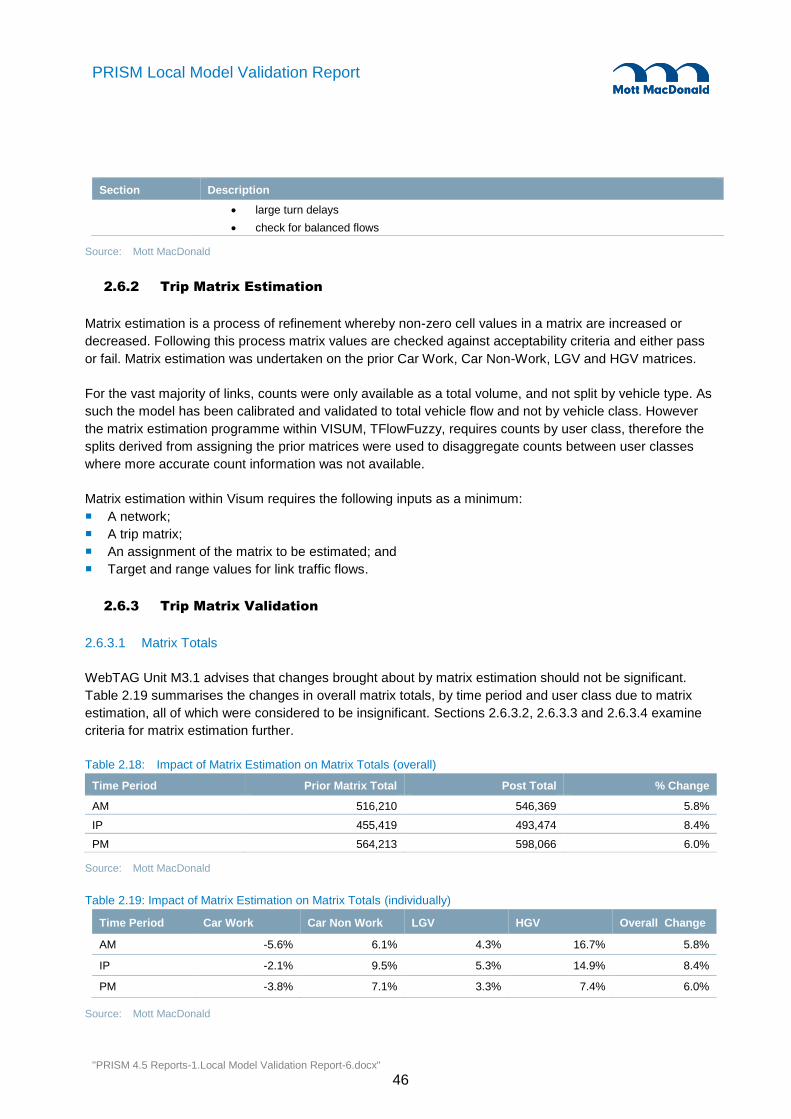
"PRISM 4.5 Reports-1.Local Model Validation Report-6.docx"
46
PRISM Local Model Validation Report
Section Description
large turn delays
check for balanced flows
Source: Mott MacDonald
2.6.2 Trip Matrix Estimation
Matrix estimation is a process of refinement whereby non-zero cell values in a matrix are increased or
decreased. Following this process matrix values are checked against acceptability criteria and either pass
or fail. Matrix estimation was undertaken on the prior Car Work, Car Non-Work, LGV and HGV matrices.
For the vast majority of links, counts were only available as a total volume, and not split by vehicle type. As
such the model has been calibrated and validated to total vehicle flow and not by vehicle class. However
the matrix estimation programme within VISUM, TFlowFuzzy, requires counts by user class, therefore the
splits derived from assigning the prior matrices were used to disaggregate counts between user classes
where more accurate count information was not available.
Matrix estimation within Visum requires the following inputs as a minimum:
A network;
A trip matrix;
An assignment of the matrix to be estimated; and
Target and range values for link traffic flows.
2.6.3 Trip Matrix Validation
2.6.3.1 Matrix Totals
WebTAG Unit M3.1 advises that changes brought about by matrix estimation should not be significant.
Table 2.19 summarises the changes in overall matrix totals, by time period and user class due to matrix
estimation, all of which were considered to be insignificant. Sections 2.6.3.2, 2.6.3.3 and 2.6.3.4 examine
criteria for matrix estimation further.
Table 2.18: Impact of Matrix Estimation on Matrix Totals (overall)
Time Period Prior Matrix Total Post Total % Change
AM 516,210 546,369 5.8%
IP 455,419 493,474 8.4%
PM 564,213 598,066 6.0%
Source: Mott MacDonald
Table 2.19: Impact of Matrix Estimation on Matrix Totals (individually)
Time Period Car Work Car Non Work LGV HGV Overall Change
AM -5.6% 6.1% 4.3% 16.7% 5.8%
IP -2.1% 9.5% 5.3% 14.9% 8.4%
PM -3.8% 7.1% 3.3% 7.4% 6.0%
Source: Mott MacDonald

"PRISM 4.5 Reports-1.Local Model Validation Report-6.docx"
47
PRISM Local Model Validation Report
2.6.3.2 Matrix Zonal Cell Values
Table 2.20 summarises the change brought about by matrix estimation for each time period at the matrix
OD cell level. TAG Unit 3.19 (M3.1) states the following targets for zonal cell values:
Slope within 0.98 and 1.02;
Intercept near 0; and
R2 in excess of 0.95.
Table 2.20: Monitoring zonal cell values
Time period Gradient Intercept R2
AM 1.00 0.029 0.96
IP 1.01 0.033 0.97
PM 1.01 0.029 0.96
Source: Mott MacDonald
2.6.3.3 Matrix Zonal Trip Ends
Table 2.21 summarises the change brought about by matrix estimation for each matrix for trip origins. TAG
Unit 3.19 (M3.1) states the following criteria for matrix zonal trip ends:
Gradient between 0.99 and 1.01;
Intercept near 0; and
R2 in excess of 0.98.
Table 2.21: Monitoring zonal trip ends – origins
Time period Gradient Intercept R2
AM 0.99 36.78 0.95
IP 1.01 35.80 0.96
PM 1.00 36.63 0.96
Source: Mott MacDonald
Table 2.22 summarises the change brought about by matrix estimation for all matrices for trip destinations.
Table 2.22: Monitoring zonal trip ends – destinations
Time period Gradient Intercept R2
AM 0.99 36.42 0.96
IP 1.01 33.48 0.96
PM 1.00 37.07 0.96
Source: Mott MacDonald
Clearly most of the criteria are close to the WebTAG guidelines. Those that exceeded the criteria were
examined and a judgement was made as to whether they were important or not. Trips origins and
destinations in the extreme ends of the model and those not in the FMA are less important; hence we have
some deviation from the target criteria. Values in both prior and post matrices range from 0 to over 3000,
hence we can conclude that proportionately, the intercepts are close to zero.

"PRISM 4.5 Reports-1.Local Model Validation Report-6.docx"
48
PRISM Local Model Validation Report
2.6.3.4 Trip Length Distribution
The following figures illustrate the trip length distribution before and after matrix estimation.
Figure 2.10: AM Car Work
Source: Mott MacDonald
Figure 2.11: AM Car Non Work
Source: Mott MacDonald

"PRISM 4.5 Reports-1.Local Model Validation Report-6.docx"
49
PRISM Local Model Validation Report
Figure 2.12: AM LGV
Source: Mott MacDonald
Figure 2.13: AM HGV
Source: Mott MacDonald

"PRISM 4.5 Reports-1.Local Model Validation Report-6.docx"
50
PRISM Local Model Validation Report
Figure 2.14: IP Car Work
Source: Mott MacDonald
Figure 2.15: IP Car Non Work
Source: Mott MacDonald

"PRISM 4.5 Reports-1.Local Model Validation Report-6.docx"
51
PRISM Local Model Validation Report
Figure 2.16: IP LGV
Source: Mott MacDonald
Figure 2.17: IP HGV
Source: Mott MacDonald

"PRISM 4.5 Reports-1.Local Model Validation Report-6.docx"
52
PRISM Local Model Validation Report
Figure 2.18: PM Car Work
Source: Mott MacDonald
Figure 2.19: PM Car Non Work
Source: Mott MacDonald
Figure 2.20: PM LGV

"PRISM 4.5 Reports-1.Local Model Validation Report-6.docx"
53
PRISM Local Model Validation Report
Source: Mott MacDonald
Figure 2.21: PM HGV
Source: Mott MacDonald

"PRISM 4.5 Reports-1.Local Model Validation Report-6.docx"
54
PRISM Local Model Validation Report
Table 2.23 shows the mean trip length for each matrix before and after matrix estimation.
Table 2.23: Mean trip lengths (km)
Car Work Car Non Work LGV HGV
Prior Post % Diff Prior Post % Diff Prior Post % Diff Prior Post % Diff
AM 52.0 58.6 13% 17.8 17.0 -5% 40.9 41.6 2% 50.8 51.3 1%
IP 57.7 62.8 9% 14.2 13.5 -5% 39.7 39.6 0% 52.5 51.7 -1%
PM 56.5 63.7 13% 16.6 15.6 -5% 39.6 39.9 1% 66.5 68.8 3%
Source: Insert source text here
2.6.4 Assignment Calibration
2.6.4.1 Traffic Flows: Screenlines
The following screenlines have been used within the calibration of the highway matrices:
RSI screenlines;
District screenlines; and
Other calibration screenlines.
The location of these screenlines is given in Figure 2.22.
Figure 2.22: Location of calibration screenlines
Source: Mott MacDonald
Modelled and observed traffic flows have been compared for all calibration screenlines. The relative
difference between modelled and observed flows is summarised in Table 2.24 and Table 2.25.

"PRISM 4.5 Reports-1.Local Model Validation Report-6.docx"
55
PRISM Local Model Validation Report
Table 2.24: Calibration screenline results – relative difference
Percentage of screenlines within relative difference of:
Time period
Type Count 1% 2% 3% 4% 5% 6% 7% 8% 9% 10%
AM RSI 34 44% 68% 79% 88% 88% 91% 97% 97% 97% 97%
District 36 58% 78% 92% 94% 94% 97% 97% 97% 97% 97%
Other 46 39% 48% 63% 83% 83% 87% 89% 91% 91% 93%
All 116 47% 63% 77% 88% 88% 91% 94% 95% 95% 96%
IP RSI 34 62% 68% 82% 91% 94% 97% 97% 97% 100% 100%
District 36 58% 89% 94% 94% 94% 94% 94% 94% 97% 97%
Other 46 37% 61% 76% 85% 91% 91% 93% 93% 93% 96%
All 116 51% 72% 84% 90% 93% 94% 95% 95% 97% 97%
PM RSI 34 50% 79% 79% 82% 85% 88% 91% 94% 94% 94%
District 36 44% 53% 78% 86% 92% 100% 100% 100% 100% 100%
Other 46 37% 52% 70% 74% 78% 89% 93% 96% 96% 98%
All 116 43% 60% 75% 80% 84% 92% 95% 97% 97% 97%
Source: Mott MacDonald
Table 2.25: Calibration screenline results – GEH
Percentage of screenlines within GEH of:
Time period
Type Count 1 2 3 4 5 6 7 8 9 10
AM RSI 34 68% 91% 100% 100% 100% 100% 100% 100% 100% 100%
District 36 83% 97% 97% 97% 100% 100% 100% 100% 100% 100%
Other 46 59% 83% 91% 96% 96% 98% 100% 100% 100% 100%
All 116 69% 90% 96% 97% 98% 99% 100% 100% 100% 100%
IP RSI 34 79% 94% 100% 100% 100% 100% 100% 100% 100% 100%
District 36 86% 94% 94% 97% 100% 100% 100% 100% 100% 100%
Other 46 67% 87% 89% 98% 98% 98% 98% 98% 100% 100%
All 116 77% 91% 94% 98% 99% 99% 99% 99% 100% 100%
PM RSI 34 79% 85% 94% 94% 94% 97% 100% 100% 100% 100%
District 36 56% 81% 94% 100% 100% 100% 100% 100% 100% 100%
Other 46 59% 74% 89% 93% 96% 96% 98% 100% 100% 100%
All 116 64% 79% 92% 96% 97% 97% 99% 100% 100% 100%
Source: Mott MacDonald
The above tables illustrate that calibration screenline flows are within 5% of the observed in nearly all
cases as required by WebTAG M3.1 criteria.
It should be noted that the GEH criteria for calibration and validation is no longer current, however it still
remains to be a sound method for checking the level of fit of a model.
Further detail, including pass/fail plots of calibration screenlines, is provided in Appendix D.

"PRISM 4.5 Reports-1.Local Model Validation Report-6.docx"
56
PRISM Local Model Validation Report
2.6.4.2 Traffic Flows: Individual Links
A comparison of modelled and observed flow on individual calibration links was also undertaken. These
links are those that:
Fall on RSI, district or other calibration screenlines;
Are on journey time routes; and
Are stand-alone counts on roads of strategic importance.
The location of these counts is illustrated in Figure 2.23.
Figure 2.23: Location of calibration counts
Source: Mott MacDonald
Table 2.26 summarises the level of fit between modelled and observed traffic counts against the WebTAG
3.19 M3.1 criteria.
Table 2.26: Calibration link results –WebTAG criteria
Time period Counts Pass Pass (%)
AM 1901 1633 86%
IP 1901 1712 90%
PM 1901 1653 87%
Source: Mott MacDonald

"PRISM 4.5 Reports-1.Local Model Validation Report-6.docx"
57
PRISM Local Model Validation Report
Table 2.27: Calibration link results – extended WebTAG criteria (allow GEH <= 7.5)
Time period Counts Pass Pass (%)
AM 1901 1747 92%
IP 1901 1806 95%
PM 1901 1771 93%
Source: Mott MacDonald
The above tables show that the modelled flows compare well to the observations in all three time periods.
Pass/fail plots of individual calibration links and comparison against count data can be found Appendix D.
2.6.5 Assignment Validation
2.6.5.1 Traffic Flows: Screenlines
In all, thirteen screenlines were retained for independent validation as illustrated in Figure 2.24.
Figure 2.24: Location of screenlines retained for independent validation
Source: Mott MacDonald
Modelled and observed traffic flow have been compared for all 13 validation screenlines. The relative
difference between modelled and observed is summarised in Table 2.28.
Table 2.28: Validation screenline results – relative difference
Percentage of screenlines within relative difference of:
Time period
Count 1% 2% 3% 4% 5% 6% 7% 8% 9% 10%
AM 32 9% 16% 25% 38% 50% 63% 66% 72% 78% 81%
IP 32 25% 28% 41% 53% 59% 63% 75% 78% 78% 81%
PM 32 16% 25% 34% 47% 56% 72% 72% 81% 84% 84%
Source: Mott MacDonald
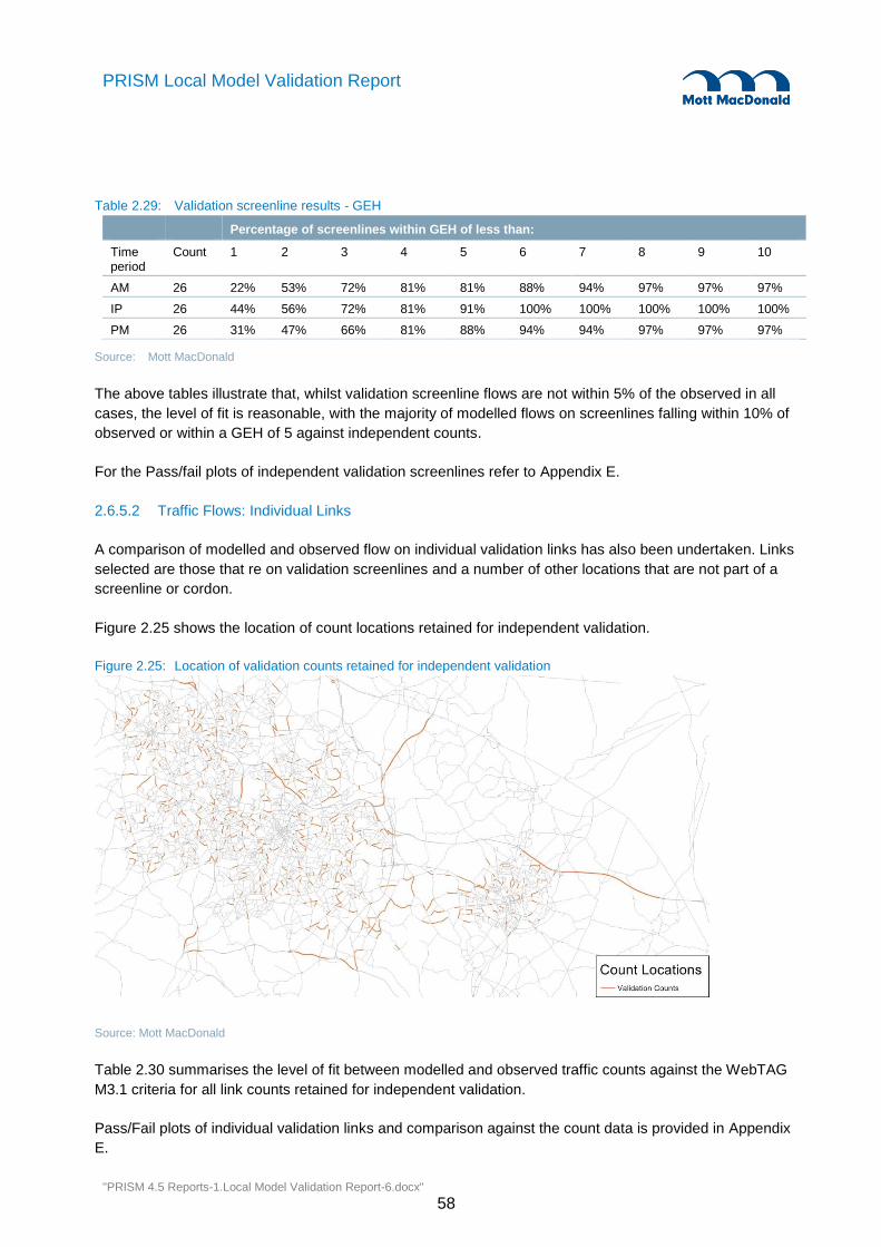
"PRISM 4.5 Reports-1.Local Model Validation Report-6.docx"
58
PRISM Local Model Validation Report
Table 2.29: Validation screenline results - GEH
Percentage of screenlines within GEH of less than:
Time period
Count 1 2 3 4 5 6 7 8 9 10
AM 26 22% 53% 72% 81% 81% 88% 94% 97% 97% 97%
IP 26 44% 56% 72% 81% 91% 100% 100% 100% 100% 100%
PM 26 31% 47% 66% 81% 88% 94% 94% 97% 97% 97%
Source: Mott MacDonald
The above tables illustrate that, whilst validation screenline flows are not within 5% of the observed in all
cases, the level of fit is reasonable, with the majority of modelled flows on screenlines falling within 10% of
observed or within a GEH of 5 against independent counts.
For the Pass/fail plots of independent validation screenlines refer to Appendix E.
2.6.5.2 Traffic Flows: Individual Links
A comparison of modelled and observed flow on individual validation links has also been undertaken. Links
selected are those that re on validation screenlines and a number of other locations that are not part of a
screenline or cordon.
Figure 2.25 shows the location of count locations retained for independent validation.
Figure 2.25: Location of validation counts retained for independent validation
Source: Mott MacDonald
Table 2.30 summarises the level of fit between modelled and observed traffic counts against the WebTAG
M3.1 criteria for all link counts retained for independent validation.
Pass/Fail plots of individual validation links and comparison against the count data is provided in Appendix
E.
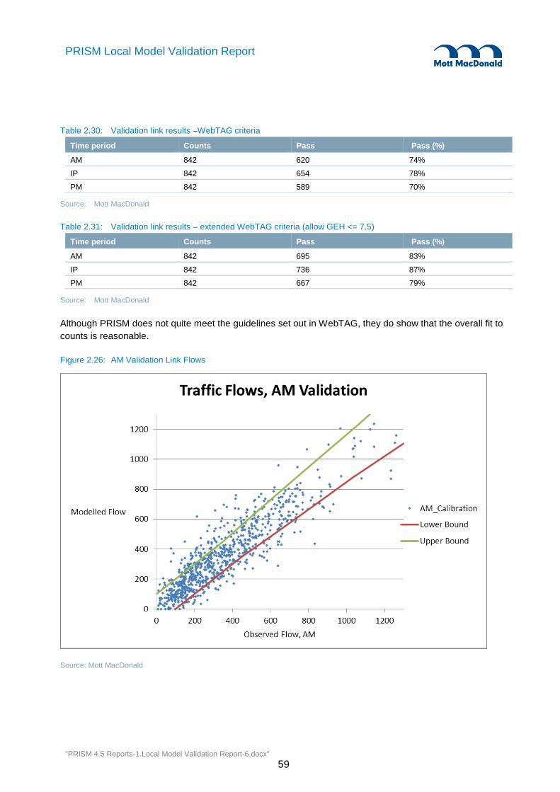
"PRISM 4.5 Reports-1.Local Model Validation Report-6.docx"
59
PRISM Local Model Validation Report
Table 2.30: Validation link results –WebTAG criteria
Time period Counts Pass Pass (%)
AM 842 620 74%
IP 842 654 78%
PM 842 589 70%
Source: Mott MacDonald
Table 2.31: Validation link results – extended WebTAG criteria (allow GEH <= 7.5)
Time period Counts Pass Pass (%)
AM 842 695 83%
IP 842 736 87%
PM 842 667 79%
Source: Mott MacDonald
Although PRISM does not quite meet the guidelines set out in WebTAG, they do show that the overall fit to
counts is reasonable.
Figure 2.26: AM Validation Link Flows
Source: Mott MacDonald

"PRISM 4.5 Reports-1.Local Model Validation Report-6.docx"
60
PRISM Local Model Validation Report
Figure 2.27: IP Validation Link Flows
Source: Mott MacDonald
Figure 2.28: PM Validation Link Flows
Source: Mott MacDonald

"PRISM 4.5 Reports-1.Local Model Validation Report-6.docx"
61
PRISM Local Model Validation Report
2.6.6 Journey Times
Modelled journey times have been compared against TM observed journey times for 80 routes (40 routes in
two directions). These routes are illustrated in Figure 2.29.
Table 2.32 summarises how the modelled and observed journey times compare. Individual route
comparisons are provided in Appendix F.
Table 2.32: Journey time validation
Time period % within 1 minute or 15%
AM 83%
IP 81%
PM 81%
Source: Mott MacDonald
The table shows that the journey time validation is good for all three time periods, with over 80% of routes
passing the M3.1 criteria in all three time periods. In the majority of cases where journey times do not
validate the modelled journey time is less than the observed. This is likely due to:
During the calibration process junction coding was calibrated to reduce overall network delay and
queuing on links, which in turn brought about more accurate traffic flows and assignment convergence.
This reduction in junction delay may have led to lower journey times; and
Figure 2.29: Journey time routes
Source: Mott MacDonald
2.6.7 Assignment Convergence
The convergence criteria are described in Section 2.1.2, and Table 2.4 is repeated below for ease of
reference:

"PRISM 4.5 Reports-1.Local Model Validation Report-6.docx"
62
PRISM Local Model Validation Report
Table 2.4: Highway assignment convergence criteria
Description of test Acceptability guideline
Overall Assignment:
1 The link volumes from the current embedded assignment and the previous embedded assignment are close
More than 95% of links have a difference in delay less than GEH 1
2 The turn volumes from the current embedded assignment and the previous embedded assignment are close
More than 95% of turns have a difference in delay less than GEH 1
3 The turn volumes from the current embedded assignment and the “smoothed” turn volumes used in ICA close
More than 95% of turns have a difference in delay less than GEH 1
4 The final link delays from the embedded assignment and those obtained from running ICA/Blocking Back are close, i.e. testing if the link VDFs are a good estimate of delay
More than 90% of turns have a relative difference in delay less than 5%
5 The final turn delays from the embedded assignment and those obtained from running ICA/Blocking Back are close, i.e. testing if the turn VDFs are a good estimate of delay
More than 90% of turns have a relative difference in delay less than 5%
6 The mean deviation in queue lengths on links is sufficiently small i.e. the queues have stabilised.
Less than 1 vehicle
Embedded Assignment:
7 DELTA: The difference between the costs along the chosen routes and those along the minimum cost routes, summed across the whole network, and expressed as the percentage of the minimum costs (referred to as ‘delta’ in TAG unit M3-1 section C.2.4)
Less than 0.0001%
Source: PTV advice on Visum assignment with ICA
As is recommended by WebTAG, the models performance against the criteria have been recorded for the
final four consecutive iterations, this is shown in Table 2.33 below:
Table 2.33: PRISM 2011 v4.5 Highway Convergence Results
Time period
Number of iterations Criteria 1 Criteria 2 Criteria 3 Criteria 4 Criteria 5 Criteria 6 Criteria 7
AM 6 93% 90% 98% 98% 93% 1.2 1.2E-06
AM 7 95% 94% 99% 99% 95% 1.0 9.3E-07
AM 8 97% 95% 99% 99% 96% 0.8 9.0E-07
AM 9 98% 96% 99% 99% 97% 0.6 8.3E-07
IP 4 85% 82% 95% 98% 86% 2.0 7.8E-07
IP 5 93% 90% 98% 99% 92% 1.3 9.2E-07
IP 6 96% 94% 99% 99% 95% 0.9 8.8E-07
IP 7 97% 95% 99% 99% 96% 0.6 6.7E-07
PM 6 92% 89% 98% 98% 92% 1.3 9.5E-07
PM 7 94% 92% 98% 99% 94% 1.0 7.5E-07
PM 8 96% 94% 99% 99% 95% 0.9 8.5E-07
PM 9 97% 96% 99% 99% 96% 0.8 8.1E-07
TARGET - 95% 95% 95% 90% 90% 1.0 1.00E-06
Source: Mott MacDonald

"PRISM 4.5 Reports-1.Local Model Validation Report-6.docx"
63
PRISM Local Model Validation Report
The above tables show that the level of convergence achieved for all three highway models successfully
meet the standards for the highway assignment.
During initial model application, MM developed a process to calculate the assignment %GAP (as defined in
WebTAG). The target in WebTAG is <0.1%, however the results were 0.71% (AM), 0.60% (IP) and 0.89%
(PM). This result led to further work being carried out on model convergence which culminated in PRISM
4.6.
For further details on how the %GAP has been calculated, and how MM have improved the convergence
please see PRISM 4.6 reporting.
2.7 Summary
2.7.1 Model Development
The PRISM 2011 highway models have been developed using Visum version 15 as a basis for travel
demand forecasting. The models have been built with a tiered level of detail, with detailed junction coding
in the Area of Detailed Modelling, speed/flow curves within the Rest of the Fully Modelled Area and
relatively fixed speeds within the external area. The highway models described in this report incorporate
blocking back and the associated flow metering effects within the AoDM, allowing for the more accurate
modelling of route choice.
The model includes two car vehicle-classes, LGV and HGV. The models have been built in line with TAG
Unit M3.1 guidance for the AM, IP and PM time periods for an average weekday.
Data collected for the development of the base year highway models included Census journey to work
matrices, RSI surveys to cover trip patterns for all user classes, Trafficmaster data for high mileage drivers,
INRIX data for goods vehicle trip patterns, 2011 household travel survey data for travel behaviour,
automatic and manual traffic counts for link volume flows and journey time route data.
2.7.2 Standards Achieved
TAG M3.1 criteria were used to assess the performance of the highway models in terms of link volumes,
journey times, screenlines, and changes brought about by matrix estimation and convergence.
Whilst the model does not meet or exceed all validation criteria in all cases, the final models validate well
against TAG criteria, given the size of the model and the quality of the trip matrix has not been
compromised to meet the guideline validation criteria.

"PRISM 4.5 Reports-1.Local Model Validation Report-6.docx"
64
PRISM Local Model Validation Report
3.1 Model Standards
3.1.1 Validation Criteria and Acceptability Guidelines
Guidance for the calibration and validation of the PRISM Public Transport Assignment Model (PTAM) was
taken from WebTAG unit M3.2. This provides criteria for three types of validation:
Validation of the trip matrix;
Network and service validation; and
Assignment validation.
Validation of the trip matrix involves comparing modelled flow and observed count values across complete
screenlines. The criterion states that in 95% of cases modelled flows should be within 15% of observed
counts.
Network and service validation refers to checks completed on the link geometry and comparisons of
modelled and observed values on individual services. Since there are no specific guidelines on these
checks, best practice was followed by checking and validating coding and modelled journey times against
those timetabled.
Assignment validation refers to comparison of flows on links on screenlines with observed data and also
comparison of boardings and alightings in urban centres. In this case flows across modelled screenlines
should be within 15% of observed counts and on individual links within the network flows should be within
25% of counts except where the observed flows are below 150 during the assignment period. WebTAG
does not define the criteria in the case where observed flows are below 150. Therefore a comparison
between flows and counts is not made. The criterion applied in calibration is further explained in section
3.7.1.
Data used for calibration and validation is detailed in section 3.4. The standards achieved and processes
undertaken during calibration and validation are given in section 3.7.
3.2 Key Features in PRISM 4.5
PRISM 4.1 PT assignment were headway-based and used VISUM 12.5, which can lead to some
unrealistic cost changes between a do-minimum and do-something test scenario. In particular it was
found that sometimes network improvements produced output costs quantifiably worse which in turn
made scheme appraisal very difficult. PRISM 4.5 is timetable-based and uses new functionality that we
specifically requested in VISUM 15, to address this issue
PRISM 4.5 demand model has been re-calibrated using more data to better represent sub-mode choice
between rail and metro.
PRISM 4.5 PT assignment demand is now segmented by PT sub-mode (bus, metro, rail)
Since PRISM 4.1, a lot of the network structure within the PTAM has remained constant, the two main
changes relate to the segmentation of user classes and assignment methodology. These are described in
more detail below.
In addition to this some changes to the trip matrix build were made, to make use of the Census journey to
work data, this is recorded within section 3.6.
3 Public Transport

"PRISM 4.5 Reports-1.Local Model Validation Report-6.docx"
65
PRISM Local Model Validation Report
3.2.1 User Classes
In PRISM 4.1 there were three demand segments included in the model, and each demand segment was
allowed to use any bus, metro or train service:
The Fare and No Fare demand segments included all trips between any zones in the FMA; and
The PLD (Planet Long Distance) demand segment contains demand to or from external area zones.
The Fare demand segment was for passengers who pay full cash fares for each service boarded. The No
Fare demand segment assumed that no fares are paid at the point of use and represented season ticket
and concessionary fares. Therefore a passenger who pays for a season ticket or a concessionary fare pays
no fare in the assignment. For more information on the relevance of fares within the model see section
3.3.7.
The PLD demand segment is based on data available from the PLD model. For more information see
section 3.6.5.
In order to provide better integration with the demand model, it became clear that for PRISM 4.5, it would
be helpful to segment demand between bus, metro and train, using the following hierarchy:
Train,
If a trip uses a rail component, then it is classified as a train trip, and any metro or bus components are
considered as access to train.
Metro,
If a trip uses a metro component, and no train component, then it is classified as a metro trip. Any bus
component is considered as access to the metro line.
Bus,
If a trip uses exclusively bus services, then it is considered a bus trip.
Using this hierarchy the following 7 user classes were defined:
Train Fare,
Metro Fare,
Bus Fare,
Train No Fare,
Metro No Fare,
Bus No Fare,
PLD (Planet Long Distance)
The distinction between fare and no-fare is consistent with PRISM 4.1, and the ratios defined in Table 3.5.
Apart from the synethic trip matrices, demand data was not available in this segmentation – nor could count
data be characterised in the way for practical reasons. Consequently it was decided to calibrate the model
using fewer user classes (as in PRISM 4.1), and to then to split the non-PLD demand across the other
user-classes according to what proportion of trips is predicted to use Bus/Metro/Train paths. This is
described in more detail in 3.2.2.1 below.
3.2.1.1 TfWM use of the model
It was noted that TfWM (formerly CENTRO) would likely have a requirement to run multiple assignments
using fixed demand – and the additional segmentation in user classes required by the PRISM demand
model would add to the run-time unnecessarily. As such it was proposed that for simple tests, TfWM would
sum up the Fare and No Fare matrices into the traditional 3 user-classes, to enable quicker assignments.

"PRISM 4.5 Reports-1.Local Model Validation Report-6.docx"
66
PRISM Local Model Validation Report
This will not affect base year validation due to the way base year demand was calibrated and then
segregated into the 7 user-classes.
3.2.2 Assignment Methodology
The assignment methodology in PRISM 4.1 made use of the headway based assignment and parameters
provided in the Visum software. The decision to use this, rather than the timetable based method was
informed by the large scale of the model, the high proportion of high frequency services, the need to have
sensible model run times.
However following a number of tests during model application, and consultation with PTV, it became clear
that many services (particularly rail) were not sufficiently high frequency for the headway assignment to be
suitable. This was observed in the calculation of transfer wait times at stations, as this became highly
unstable in many cases (in some cases causing large dis-benefits to travel time to appear when adding a
new service). To remedy this instability the model was converted to use timetable assignments – where
routes are picked based on the timetabled services available in the assignment interval. In this way transfer
times are calculated exactly rather than approximated, for example a transfer at Birmingham New Street
between a service the arrives at 8.46am and another that departs and 8.59am will always be 13min –
however when using the headway methodology the relative frequency of the two services along with all
other services that may be picked at that stop are taking into account – making the final result unstable due
to dependence on other services. In smaller ‘mid-sized’ networks this impact is relatively small and can be
monitored carefully, however for PRISM the network was so large that it was not practicable to review
every transfer (or even a representative sample).
The timetable methodology produced route flows that were similar to the headway assignment, and thanks
to innovations in PTV Visum 15, run-times although longer were still reasonable.
3.2.2.1 Sub-mode assignment – COFEE
In order to assign the separate user-classes observing the Train/Metro/Bus hierarchy described in 3.2.1,
MM have developed a new python package COFEE (COnnection File External Editor). The COFEE
process is as follows:
1. Perform an assignment of a matrix of 1s, allowing all sub-modes to be used. This demand is then
exported by visum into external connection files, detailing the various routes and PT services used for
each path for each OD.
2. The main COFEE module is run, this reads in all the paths found by the assignment and categorises
them as either Train, Metro or Bus, respecting the hierarchy described in 3.2.1. The output is 3
separate connection files containing the appropriate paths.
3. Further assignments of demand will then read in paths from the connection files, with VISUM
distributing demand across the paths based on the relative impedances of routes.
Using the above process, the assignments are able to provide skims to the demand model at the sub-mode
level, and are able to assign the forecast demand matrices to the relevant sub-mode categories. This last
feature is particularly important as it means the growth (or decline) in a particular sub-mode in the
assignment mirrors that predicted by the demand model (which will have taken many demographic factors
into account in addition to relative journey times).

"PRISM 4.5 Reports-1.Local Model Validation Report-6.docx"
67
PRISM Local Model Validation Report
3.3 Key Features
3.3.1 Fully Modelled Area and External Area
The PRISM PTAM has similar network coverage to the PRISM HAM, with the same boundary definitions
for the FMA (AoDM and RotFMA) and External areas as described in section 2.2.1. Key features of those
areas in relation to the PTAM are as follows:
Fully modelled area (FMA). The fully modelled area is subdivided into:
Area of detailed modelling (AoDM) - Modelling in this area is characterised by smaller zones, a
detailed link and node network, extra detail within urban centres and all PT services; and
Rest of the fully modelled area (RotFMA) – Modelling in this area is characterised by somewhat
larger zones, straight line links between bus stops and all PT services.
External area. Modelling in this area is characterised by a skeletal network, large zones and only
external demand through or with one trip end in the FMA represented. The rail network has been
simplified in this area to account for the partially represented demand and only PT services which pass
into the FMA are included.
3.3.2 Zoning System
The PRISM PTAM zoning system has essentially been constructed by combining the AoDM zones from the
Centro 2005/2008 model and the RotFMA and external area zones from the HAM zoning system (see
section 2.2.2). Within the AoDM there is a correspondence between the PTAM and HAM zoning systems
and typically three to five PTAM zones fit into a HAM zone.
To account for cases where PRISM HAM zones overlapped Centro zones and where more accurate land
use modelling was required, five adjustments were made to the PTAM zoning system in the AoDM:
A zone in Walsall town centre has been split into two parts;
The zone containing the proposed Curzon Street HS2 station has been split into two parts; and
Three zones in Sandwell have each been split into two parts.
Table 3.1 gives an overview of the zoning system. For detail on centroids and connectors see section
3.3.4.
Table 3.1: Overview of Zoning System
System Area Frequency Comment
PRISM PTAM All 1900
Polygon 1855 Non Park and Ride Zones
Point 45 Park and Ride Zones
From Centro 2005/2008 Model
(including the five adjustments above and Park and Ride zones)
Birmingham 512
Sum = 1603
Coventry 204
Dudley 170
Sandwell 179
Solihull 154
Walsall 150
Wolverhampton 189
Park and Ride 45
PRISM HAM Intermediate 254

"PRISM 4.5 Reports-1.Local Model Validation Report-6.docx"
68
PRISM Local Model Validation Report
System Area Frequency Comment
Rest of WM 20 Sum = 297
External 23
Figure 3.1 below shows the zoning system within the AoDM area to give an example of the level of detail
that it contains.
Figure 3.1: PTAM zones in the Area of Detailed Modelling
Source: Mott MacDonald
3.3.3 Network Structure
This section gives a brief description of the network structure. For further information see section 3.5.
Historically the PRISM HAM and the PRISM/Centro PTAMs contained different link and node topology. As
a result of this there is no direct correspondence between links or nodes between the PRISM HAM and
PTAM. See section 3.3.9 for more detail on the relationship between the two models.
The network structure of the PRISM PTAM is based on the Centro 2005/2008 PT model. It contains the
following:
A detailed link network within the AoDM, taken from Centro’s 2005/2008 model which was originally
built on the 2001 OS OSCAR road network dataset;
A less detailed link network outside of the AoDM where only straight links exist between PT stops;
A large number of links included within the urban areas of the AoDM which are used to model
passengers walking to and between services; and
A rail and Midland Metro network coded separately to the bus network with a realistic representation of
the actual rail and Metro services. Only the rail lines which are relevant to the model are included.
There are no changes to the link and node network since 2005. This is because any major highway
changes have not significantly affected bus routes and only small revisions have been made during the

"PRISM 4.5 Reports-1.Local Model Validation Report-6.docx"
69
PRISM Local Model Validation Report
checking stages. The implications of any highway changes are reflected in modelled journey times, as the
2011 bus timetable data will include the stop to stop scheduled service times.
3.3.4 Centroid Connectors
Zone centroids have been coded based on the location of population within each zone in a similar way to
the PRISM HAM (see 2.2.4).
In the PRISM PTAM a connector will generally represent the path a person takes to walk on to the network.
The following assumptions have been used to add connectors into the network:
Where possible, connectors have been coded such that they do not cross barriers to movement, i.e.
rivers, railways and major roads such as motorways;
Where possible, several connectors are coded from each zone to model the choice of services
available;
At least one PT service should be accessible from any zone in at least one of the modelled time
periods;
The length of connectors has been multiplied by 1.2 to represent the bendiness of roads;
The travel time along any connector is limited to 15 minutes and all connector distances are limited to
1km. This is generally applied in the RotFMA and external areas since catchment areas have been
defined for the AoDM; and
Where possible consecutive stops of a service are not joined to the same zone via a connector.
A catchment area has been set for each mode of travel within the AoDM:
Bus 400m
Midland Metro 600m
Heavy Rail 800m
This helps to improve access and to model realistic mode choices.
3.3.5 Time Periods
The services within the PRISM PTAM represent an average weekday in October 2011. The demand
assigned to the networks represents an average weekday (during school term) in 2011. The following 2-
hour time periods are represented in the PRISM PTAMs:
AM; 0700-0900
IP; 1000-1200
PM; 1600-1800.
Again like the PRISM Highway Assignment Model (2.2.5), the OP time period (1900-0700) is not modelled
explicitly. It is felt any scheme being tested will only have negligible benefits in this time period, so was not
needed.
3.3.6 Crowding
The issue of whether to include a representation of the impacts of crowded conditions on public transport
vehicles was considered in detail. The topic was reviewed and advice was sought from various parties
including the Department for Transport at the beginning of 2013.

"PRISM 4.5 Reports-1.Local Model Validation Report-6.docx"
70
PRISM Local Model Validation Report
While recognising that crowding does occur on the West Midlands rail network, and on Midland Metro Line
One, the decision was taken not to model crowding in the PTAM. This view was informed by a number of
factors:
There is a lack of observed data available – particularly for the bus network;
Other models held by Centro are capable of modelling crowding (e.g. Radform model based on PDFH
crowding costs and elasticities);
Model outputs can be checked against capacity, with crowding changes for future scenarios calculated
through post assignment processing; and
The Visum software does not provide functionality to model crowding in an acceptable way using the
headway assignment method, without introducing a number of model loops, which would impact
severely on run times.
In order to future-proof the model a method has been identified which will allow crowding costs to be
included but would require re-estimation of the PRISM Demand Model.
3.3.7 Fares
Fares are only taken into account by passengers who belong to a Fare demand segment. Season tickets
and concessionary fares such as all-day fares or return fares were not taken into account. Therefore, only
data related to single cash fares was collected.
Fare is coded in the PTAM in two parts which are added together to calculate the total fare:
A boarding fare, which is paid by passengers when they board a service in the model; and
A distance based fare, which is incurred by a passenger based on the distance they travel.

PRISM 4.5 Reports-1.Local Model Validation Report-6.docx
71
PRISM Local Model Validation Report
PRISM 4.5
Passengers boarding a bus service pay a fee of £1.80 and they do not pay a distance based fare. This price has been chosen as it was the National Express
West Midlands price for a single ticket in 2011. Train and Metro services include a boarding fare as well as a distance based fare.
The fare points for Metro have been calculated using a fare matrix which uses Microsoft Excel solver to best fit a linear distance based fare with the actual fare
matrix. Table 3.2 and Table 3.3 show the actual fare matrix used and the fare points calculated by Microsoft Excel solver.
Table 3.2: Midlands Metro Fares
Snow
Hill
St P
aul's
Jew
elle
ry Q
uart
er
Soho B
enson
Ro
ad
Win
so
n G
ree
n
Hand
sw
ort
h B
oo
th
Str
ee
t
Th
e H
aw
thorn
s
Kenrick P
ark
Trinity W
ay
West B
rom
wic
h C
en
tral
Lod
ge R
oa
d
Dart
mo
uth
Str
eet
Dudle
y S
treet
Bla
ck L
ake
W’b
ury
Gre
at W
este
rn
Str
ee
t
Wedn
esb
ury
Park
way
Bra
dle
y L
an
e
Loxdale
Bils
ton C
en
tral
Th
e C
rescent
Priestfie
ld
Th
e R
oyal
St G
eorg
e's
From Stop To S
top
Snow Hill 1.90 1.90 1.90 2.60 2.60 2.60 2.60 2.60 2.60 3.30 3.30 3.30 3.30 3.30 3.30 3.30 3.30 3.30 3.30 3.30 3.30 3.30
St Paul's 1.90 1.90 1.90 2.60 2.60 2.60 2.60 2.60 2.60 3.30 3.30 3.30 3.30 3.30 3.30 3.30 3.30 3.30 3.30 3.30 3.30 3.30
Jewellery Quarter 1.90 1.90 1.90 1.90 2.60 2.60 2.60 2.60 2.60 2.60 2.60 3.30 3.30 3.30 3.30 3.30 3.30 3.30 3.30 3.30 3.30 3.30
Soho Benson Road 1.90 1.90 1.90 1.90 1.90 1.90 2.60 2.60 2.60 2.60 2.60 2.60 2.60 3.30 3.30 3.30 3.30 3.30 3.30 3.30 3.30 3.30
Winson Green 2.60 2.60 1.90 1.90 1.90 1.90 2.60 2.60 2.60 2.60 2.60 2.60 2.60 3.30 3.30 3.30 3.30 3.30 3.30 3.30 3.30 3.30
Handsworth Booth St. 2.60 2.60 2.60 1.90 1.90 1.90 1.90 1.90 2.60 2.60 2.60 2.60 2.60 2.60 3.30 3.30 3.30 3.30 3.30 3.30 3.30 3.30
The Hawthorns 2.60 2.60 2.60 1.90 1.90 1.90 1.90 1.90 1.90 2.60 2.60 2.60 2.60 2.60 2.60 3.30 3.30 3.30 3.30 3.30 3.30 3.30
Kenrick Park 2.60 2.60 2.60 2.60 2.60 1.90 1.90 1.90 1.90 1.90 1.90 2.60 2.60 2.60 2.60 3.30 3.30 3.30 3.30 3.30 3.30 3.30
Trinity Way 2.60 2.60 2.60 2.60 2.60 1.90 1.90 1.90 1.90 1.90 1.90 1.90 1.90 2.60 2.60 2.60 3.30 3.30 3.30 3.30 3.30 3.30
West Bromwich Central 2.60 2.60 2.60 2.60 2.60 2.60 1.90 1.90 1.90 1.90 1.90 1.90 1.90 2.60 2.60 2.60 2.60 3.30 3.30 3.30 3.30 3.30
Lodge Road 3.30 3.30 2.60 2.60 2.60 2.60 2.60 1.90 1.90 1.90 1.90 1.90 1.90 2.60 2.60 2.60 2.60 3.30 3.30 3.30 3.30 3.30
Dartmouth Street 3.30 3.30 2.60 2.60 2.60 2.60 2.60 1.90 1.90 1.90 1.90 1.90 1.90 2.60 2.60 2.60 2.60 3.30 3.30 3.30 3.30 3.30
Dudley Street 3.30 3.30 3.30 2.60 2.60 2.60 2.60 2.60 1.90 1.90 1.90 1.90 1.90 1.90 2.60 2.60 2.60 2.60 3.30 3.30 3.30 3.30
Black Lake 3.30 3.30 3.30 2.60 2.60 2.60 2.60 2.60 1.90 1.90 1.90 1.90 1.90 1.90 2.60 2.60 2.60 2.60 3.30 3.30 3.30 3.30
W’bury Great Western 3.30 3.30 3.30 3.30 3.30 2.60 2.60 2.60 2.60 2.60 2.60 2.60 2.60 1.90 1.90 1.90 2.60 2.60 2.60 2.60 2.60 3.30
Wednesbury Parkway 3.30 3.30 3.30 3.30 3.30 3.30 3.30 2.60 2.60 2.60 2.60 2.60 2.60 2.60 1.90 1.90 2.60 2.60 2.60 2.60 2.60 3.30
Bradley Lane 3.30 3.30 3.30 3.30 3.30 3.30 3.30 3.30 2.60 2.60 2.60 2.60 2.60 2.60 1.90 1.90 1.90 1.90 1.90 2.60 2.60 2.60
Loxdale 3.30 3.30 3.30 3.30 3.30 3.30 3.30 3.30 3.30 2.60 2.60 2.60 2.60 2.60 2.60 2.60 1.90 1.90 1.90 1.90 2.60 2.60
Bilston Central 3.30 3.30 3.30 3.30 3.30 3.30 3.30 3.30 3.30 3.30 3.30 3.30 2.60 2.60 2.60 2.60 1.90 1.90 1.90 1.90 1.90 2.60
The Crescent 3.30 3.30 3.30 3.30 3.30 3.30 3.30 3.30 3.30 3.30 3.30 3.30 3.30 3.30 2.60 2.60 1.90 1.90 1.90 1.90 1.90 2.60
Priestfield 3.30 3.30 3.30 3.30 3.30 3.30 3.30 3.30 3.30 3.30 3.30 3.30 3.30 3.30 2.60 2.60 2.60 1.90 1.90 1.90 1.90 1.90

PRISM 4.5 Reports-1.Local Model Validation Report-6.docx
72
PRISM Local Model Validation Report
PRISM 4.5
The Royal 3.30 3.30 3.30 3.30 3.30 3.30 3.30 3.30 3.30 3.30 3.30 3.30 3.30 3.30 2.60 2.60 2.60 2.60 1.90 1.90 1.90 1.90
St George's 3.30 3.30 3.30 3.30 3.30 3.30 3.30 3.30 3.30 3.30 3.30 3.30 3.30 3.30 3.30 3.30 2.60 2.60 2.60 2.60 1.90 1.90
Source: Centro
Table 3.3: Midland Metro Fare Implementation as Calculated using Microsoft Excel Solver
Fa
re P
oin
ts
Snow
Hill
St P
aul's
Jew
elle
ry Q
uart
er
Soho B
enson
Ro
ad
Win
so
n G
ree
n
Hand
sw
ort
h B
oo
th
Str
ee
t
Th
e H
aw
thorn
s
Kenrick P
ark
Trinity W
ay
West B
rom
wic
h
Centr
al
Lod
ge R
oa
d
Dart
mo
uth
Str
eet
Dudle
y S
treet
Bla
ck L
ake
W’b
ury
Gre
at W
este
rn
Str
ee
t
Wedn
esb
ury
Park
way
Bra
dle
y L
an
e
Loxdale
Bils
ton C
en
tral
Th
e C
rescent
Priestfie
ld
Th
e R
oyal
St G
eorg
e's
From Stop To S
top
Snow Hill 0.0 1.90 1.92 1.92 2.27 2.28 2.30 2.31 2.32 2.62 2.62 2.62 2.96 2.97 2.97 2.97 3.47 3.47 3.47 3.54 3.56 3.58 3.58
St Paul's 0.0 1.90 1.92 1.92 2.27 2.28 2.30 2.31 2.32 2.62 2.62 2.62 2.96 2.97 2.97 2.97 3.47 3.47 3.47 3.54 3.56 3.58 3.58
Jewellery Quarter 0.0 1.92 1.92 1.90 2.26 2.27 2.28 2.30 2.31 2.60 2.60 2.60 2.95 2.95 2.95 2.95 3.45 3.45 3.45 3.53 3.55 3.57 3.57
Soho Benson Road 0.0 1.92 1.92 1.90 2.25 2.25 2.27 2.28 2.29 2.59 2.59 2.59 2.93 2.94 2.94 2.94 3.44 3.44 3.44 3.51 3.54 3.55 3.55
Winson Green 0.4 2.27 2.27 2.26 2.25 2.25 2.27 2.28 2.29 2.58 2.59 2.59 2.93 2.94 2.94 2.94 3.44 3.44 3.44 3.51 3.53 3.55 3.55
Handsworth Booth St. 0.0 2.28 2.28 2.27 2.25 2.25 1.91 1.93 1.94 2.23 2.23 2.23 2.58 2.58 2.58 2.58 3.08 3.08 3.08 3.16 3.18 3.20 3.20
The Hawthorns 0.0 2.30 2.30 2.28 2.27 2.27 1.91 1.92 1.93 2.22 2.23 2.23 2.57 2.57 2.57 2.57 3.07 3.07 3.07 3.15 3.17 3.19 3.19
Kenrick Park 0.0 2.31 2.31 2.30 2.28 2.28 1.93 1.92 1.91 2.21 2.21 2.21 2.55 2.56 2.56 2.56 3.06 3.06 3.06 3.13 3.16 3.17 3.17
Trinity Way 0.0 2.32 2.32 2.31 2.29 2.29 1.94 1.93 1.91 2.19 2.20 2.20 2.54 2.54 2.54 2.54 3.04 3.04 3.04 3.12 3.14 3.16 3.16
West Bromwich Central 0.3 2.62 2.62 2.60 2.59 2.58 2.23 2.22 2.21 2.19 2.19 2.19 2.53 2.53 2.53 2.53 3.03 3.03 3.03 3.11 3.13 3.15 3.15
Lodge Road 0.0 2.62 2.62 2.60 2.59 2.59 2.23 2.23 2.21 2.20 2.19 1.89 2.23 2.24 2.24 2.24 2.74 2.74 2.74 2.82 2.84 2.85 2.85
Dartmouth Street 0.0 2.62 2.62 2.60 2.59 2.59 2.23 2.23 2.21 2.20 2.19 1.89 2.23 2.24 2.24 2.24 2.74 2.74 2.74 2.81 2.83 2.85 2.85
Dudley Street 0.3 2.96 2.96 2.95 2.93 2.93 2.58 2.57 2.55 2.54 2.53 2.23 2.23 2.24 2.24 2.24 2.74 2.74 2.74 2.81 2.83 2.85 2.85
Black Lake 0.0 2.97 2.97 2.95 2.94 2.94 2.58 2.57 2.56 2.54 2.53 2.24 2.24 2.24 1.90 1.90 2.40 2.40 2.40 2.47 2.49 2.51 2.51
W’bury Great Western 0.0 2.97 2.97 2.95 2.94 2.94 2.58 2.57 2.56 2.54 2.53 2.24 2.24 2.24 1.90 1.89 2.39 2.39 2.39 2.46 2.48 2.50 2.50
Wednesbury Parkway 0.0 2.97 2.97 2.95 2.94 2.94 2.58 2.57 2.56 2.54 2.53 2.24 2.24 2.24 1.90 1.89 2.39 2.39 2.39 2.46 2.48 2.50 2.50
Bradley Lane 0.5 3.47 3.47 3.45 3.44 3.44 3.08 3.07 3.06 3.04 3.03 2.74 2.74 2.74 2.40 2.39 2.39 2.39 2.39 2.46 2.48 2.50 2.50
Loxdale 0.0 3.47 3.47 3.45 3.44 3.44 3.08 3.07 3.06 3.04 3.03 2.74 2.74 2.74 2.40 2.39 2.39 2.39 1.89 1.96 1.98 2.00 2.00
Bilston Central 0.0 3.47 3.47 3.45 3.44 3.44 3.08 3.07 3.06 3.04 3.03 2.74 2.74 2.74 2.40 2.39 2.39 2.39 1.89 1.96 1.98 2.00 2.00
The Crescent 0.1 3.54 3.54 3.53 3.51 3.51 3.16 3.15 3.13 3.12 3.11 2.82 2.81 2.81 2.47 2.46 2.46 2.46 1.96 1.96 1.98 2.00 2.00
Priestfield 0.0 3.56 3.56 3.55 3.54 3.53 3.18 3.17 3.16 3.14 3.13 2.84 2.83 2.83 2.49 2.48 2.48 2.48 1.98 1.98 1.98 1.93 1.93
The Royal 0.0 3.58 3.58 3.57 3.55 3.55 3.20 3.19 3.17 3.16 3.15 2.85 2.85 2.85 2.51 2.50 2.50 2.50 2.00 2.00 2.00 1.93 1.90
St George's 0.0 3.58 3.58 3.57 3.55 3.55 3.20 3.19 3.17 3.16 3.15 2.85 2.85 2.85 2.51 2.50 2.50 2.50 2.00 2.00 2.00 1.93 1.90
Boarding Penalty 1.9
Source: Centro

PRISM 4.5 Reports-1.Local Model Validation Report-6.docx
73
PRISM Local Model Validation Report
In order to include rail fares within the model data has been sourced from Centro’s London Midlands fare
matrices and www.nationalrail.co.uk. This data has been used to plot a scatter graph of the distances of
each leg against the prices of the tickets for each leg.
A linear regression was calculated to create a linear fare based on distance. One regression line was
created for services outside of the AoDM and one was created for services inside of the AoDM. The
regression for fares outside of the AoDM was specified to have the same intercept as the within-AoDM
regression for practical reasons (to ensure that trips made within the core area regardless of train service
have comparable fare to maintain consistency on route choice).
The outcome was a rail boarding penalty of £1.39 and a fare per kilometre in the AoDM and non-AoDM of
£0.10 and £0.28 respectively. Figure 3.2 shows the regression line created based on the data available in
the AoDM.
Figure 3.2: Linear Regression for Fares in the AoDM
Source: Mott MacDonald
3.3.8 Generalised Cost Formulation
The generalised cost calculation takes into account the various legs of a passenger journey including walk
access, waiting for a service, on board time, fares, and interchanges. The various weightings of each trip

PRISM 4.5 Reports-1.Local Model Validation Report-6.docx
74
PRISM Local Model Validation Report
leg element have been calibrated as part of the overall network calibration. As an example Table 3.4 below
presents the tests conducted for the AM/PM PTAM assignment models.
Table 3.4: AM/PM PTAM generalised cost calibration
Sc
en
ari
o
VO
T
Ac
ce
ss
Tim
e
Eg
ress
Tim
e
Wa
lk T
ime
Ori
gin
Wait
Tim
e
Tra
nsfe
r W
ait
Tim
e
Tra
nsfe
r
Pe
na
lty
Wa
lk S
pee
d
IVT
Me
tro
Co
ord
ina
tio
n
Bo
ard
ing
Pe
na
lty
Fa
cto
r
Base £2.32 1.75 1.75 1.75 2.00 2.00 10mins 4.8kph 0.95 Groups 1
Test 1 £6.45 1.75 1.75 1.75 2.00 2.00 10mins 4.8kph 0.95 Groups 1
Test 2 £2.32 1.75 1.75 1.75 2.00 2.00 8mins 4.8kph 0.95 Groups 1
Test 3 £2.32 2.00 2.00 2.00 2.00 2.00 10mins 4.8kph 0.95 Groups 1
Test 4 £2.32 1.75 1.75 1.75 2.00 2.00 10mins 4.8kph 1 Groups 1
Test 5 £2.32 1.75 1.75 1.75 2.00 2.00 10mins 4.8kph 0.95 Off 1
Test 6 £2.32 1.75 1.75 1.75 2.00 2.00 10mins 4.8kph 0.95 On 1
Test 7 £2.32 1.75 1.75 1.75 2.00 2.00 10mins 6kph 0.95 Groups 1
Test 8 £2.32 1.75 1.75 1.75 2.00 2.00 10mins 4.8kph 0.95 Groups 1.5
Source: Centro
The above tests used the PT prior matrix and compared flows to observed counts to identify the optimum
settings. The final values used are shown in Table 3.5.
Table 3.5: Final PTAM generalised cost weightings by time period
Attribute AM/PM IP
VOT £2.32 £1.60
Access Time 1.75 2.5
Egress Time 1.75 2.5
Walk Time 1.75 2.5
Origin Wait Time 2 2
Transfer Wait Time 2 3
Transfer Penalty 10mins 8mins
Walk Speed 4.8kph 4.8kph
IVT Metro 0.95 0.95
IVT Rail 0.9 0.9
Fare Split AM 27%, PM 15% 18%
Source: Centro
3.3.9 Integration
The PRISM PTAM and PRISM HAM are separate assignment models but are integrated in a number of
ways. The PTAM does not react to any type of congestion on the road network however the demand model
accounts for the change in speed of buses in the future. For more information see the PRISM Forecasting
Report. The Highway network takes a bus pre-load from the PT network.

PRISM 4.5 Reports-1.Local Model Validation Report-6.docx
75
PRISM Local Model Validation Report
3.4 Calibration Data
Please see Appendix G for plots of the various calibration data described below.
3.4.1 Bus Count Data
3.4.1.1 LTP Bus Cordon Counts
Cordon counts were conducted at nine centres across the Metropolitan area:
Birmingham City Centre;
Wolverhampton City Centre;
Coventry City Centre;
Walsall Town Centre;
Dudley Town Centre;
Sutton Coldfield Town Centre;
Solihull Town Centre;
West Bromwich Town Centre; and
Brierley Hill Centre.
Conducted bi-annually at each centre, these counts capture passengers boarding, alighting and on-board
all buses between 0700 and 1230 on an average weekday. A selection of sites within each cordon is
surveyed in both directions, which provides factors by which outbound passenger flows at all sites are
calculated. To provide the PM passenger counts, the surveys conducted in 2010 and 2011 were extended
to finish at 1800.
3.4.1.2 Local Centre Cordon Counts
In building the previous Centro Public Transport model it was recognised that there is a lack of calibration
data for bus trips taking place away from LTP centres. In order to improve subsequent model builds Centro
commissioned a programme of bus cordon counts at local and district centres across the West Midlands
Metropolitan Area (WMMA). This provides passenger boarding, alighting and on-board counts for all buses
crossing the cordon. In total there are 22 local centre cordons including areas such as Harborne, Perry Barr
and Kings Heath.
3.4.1.3 Origin-Destination Survey Passenger Counts
Passenger counts were conducted alongside origin-destination surveys which have been conducted since
2005. Passenger boarding and alighting counts were processed into stop boarding and alighting flows by
time period for use in calibration. These typically form cordons of local centres or interchange sites, where
all relevant stops have been surveyed.
3.4.1.4 Bus Showcase Counts
These have been conducted in a number of corridors across the Metropolitan area over the period from
2008 to 2011 for the purposes of monitoring passenger use. They are in the same format as the bus
cordon counts and they provide boarding, alighting and on-board counts. They typically comprise a stop at

PRISM 4.5 Reports-1.Local Model Validation Report-6.docx
76
PRISM Local Model Validation Report
the outer end of the route, mid route, and at the corresponding LTP cordon site (as the majority of services
run into main centres).
3.4.1.5 Bus Station Counts
Passenger boarding and alighting counts conducted at a number of Centro operated bus stations have
been made available, processed into boarding and alighting flows.
3.4.2 Rail Count Data
3.4.2.1 LTP Centre Rail Cordon Counts
When conducting the bus LTP cordon counts, if a rail station lies within the cordon passenger boarding and
alighting counts are conducted. Passenger counts for 2010 and 2011 were available for calibrating the
2011 base year public transport model, as for the bus counts they are conducted on a bi annual
programme in the locations referred to in section 3.4.1.1.
3.4.2.2 Control Station Counts
For general rail monitoring purposes passenger boarding and alighting counts are conducted on one
weekday per month for one station on each passenger rail line. The 2011 counts have been averaged and
used in model calibration.
3.4.2.3 Local Station Passenger Counts
Subject to funding availability Centro aims to conduct a one day weekday passenger count at all local rail
stations in the WMMA once every five years. The most recent data available is from 2008/09 and this has
been used in calibration.
3.4.2.4 Park and Ride Counts
Centro conducts a monthly occupancy count at all car parks in their control. This involves a vehicle count at
around 11am on the third Thursday of each month. This is processed into passengers by means of an
average occupancy rate. They are further processed into time periods based on arrival/departure counts
conducted in 2008. As mentioned previously there are 45 park and ride sites.
3.4.2.5 PLANET Rail Counts
To fix the demand flows from the through-trip matrices, matrix estimation was carried out to fit the flows to
the link counts taken from the PLD model. For more information on the PLD model and PLD matrices used
see section 3.6.5.2. Links were chosen so that a cordon was formed around the core modelled area, so
that key links in central Birmingham where the flows are high in volume were included and so that any links
which are important in terms of model accuracy were included.
PRISM 4.5 Reports-1.Local Model Validation Report-6.docx
77
PRISM Local Model Validation Report
3.4.3 Midland Metro Count Data
An annual passenger count is conducted each October by Midland Metro, and this data is shared with
Centro. This provides a full one day count of passengers boarding and alighting at every Midland Metro
Line One stop. This data is considered suitable for calibration and has been converted into the appropriate
format for each time period.
3.5 Network
3.5.1 Data Sources
This section refers to the data sources of the network, and not the data relating to the transport matrices or
the calibration process. The public transport networks were developed jointly by Centro and Mott
MacDonald making best use of existing data held by both parties. The complete network comprises:
A link and node network based on Centro’s 2005/2008 model (originally built on the 2001 OS OSCAR
road network dataset) in the AoDM but only straight lines between stops outside of the AoDM;
Bus stops, rail stations and Midland Metro stops sourced from the NPTDR (National Public Transport
Data Repository), processed, snapped and adjusted to the appropriate location on the link and node
network; and
A network of routes representing each bus route, rail line and Midland Metro service operating in the
West Midlands on an average weekday in October 2011 from the NPTDR.
3.5.2 Timetable
Timetable data has been sourced from the NPTDR which contains the timetable data for a selected week
in October 2011 for every PT service in the UK. Data has been filtered from this data-set so that the PT
model represents trips in an average weekday.
Centro liaised with PTV, providers of the Visum software, to develop a tool for automating the process of
building public transport networks from the ATCO-CIF data. The ATCO-CIF data contains the timetable
information and the process developed by PTV takes this information to create the route information. The
final product is a public transport network file, incorporating all services including bus, rail and Midland
Metro. This network of services was then read into the base network after any additional stops were added.
Once imported a series of checks were conducted:
All routes successfully imported;
Origin and destination of services are correct;
Routes follow the correct path through the network;
Stops served by each route are correct;
Routes do not traverse the same point multiple times; and
Journey times are correct.
The route information has been checked against paper timetables and journey times using
www.networkwestmidlands.com journey planner.

PRISM 4.5 Reports-1.Local Model Validation Report-6.docx
78
PRISM Local Model Validation Report
3.6 Trip Matrix
3.6.1 Travel Demand Data
Centro and Mott MacDonald developed a programme of passenger origin-destination surveys over the
period 2009 to 2011. These surveys (comprising of passenger interviews and counts) were conducted at
main, local and district centres across the West Midlands. The surveys were conducted at stops to include
bus, rail and Midland Metro passengers.
3.6.2 Partial Trip Matrices from Surveys
The public transport demand matrices were updated by means of origin-destination surveys. Centro has a
rolling programme of annual surveys for this purpose. With the PRISM refresh it was possible to extend the
coverage of this programme by pooling resources. The programme of surveys was informed by a multi
criteria approach which took into account:
The age of the data held for a particular area (the last survey year);
The status of the location (LTP, district, local, no status);
Location of any known large development which will have impacted on travel behaviour; and
Location of any known project for which the model will be used to quantify its impact.
On the basis of the prioritisation, and making full use of resources available, 18 centres across Birmingham
and the Black Country were selected as survey locations (as shown in Appendix H). No surveys were
conducted in Coventry as a significant data collection exercise had been conducted to develop base year
matrices for the 2008 Coventry/Warwickshire public transport model. These matrices formed an input to the
prior matrix.
The data was collected in a face to face interview at stops with bus passengers, and a post back survey
form with Midland Metro and rail passengers. The two different approaches were adopted as rail and Metro
passengers typically arrive close to the departure time of their train/tram and therefore face to face sample
rates are low. The survey matrices were derived from the passenger interview returns and expanded using
the counts conducted parallel to interviews. A well-established approach is documented in further detail in
the Survey and Matrix Building Report.
Centro have historic survey data from OD matrix surveys carried out prior to the PRISM refresh
programme. These were conducted between 2005 and 2009, also being informed by the prioritisation
approach outlined above. They were converted to the 1900 zoning system from the 1418 former Centro
zoning using correspondence files agreed between Centro and Mott MacDonald.
The combination of historic and PRISM refresh surveys produced 78 site survey matrices for each time
period which fed into the matrix combination process.
3.6.3 Census 2011 Journey to Work Matrices
The Census data provides records aggregated to MSOA zones, these records contain home address and
usual place of work. Using trip rate information derived from the West Midlands Household Interviews this
information was converted into an all-day tour matrix. This was further disaggregated into PRISM zones
and into time periods using local data.

PRISM 4.5 Reports-1.Local Model Validation Report-6.docx
79
PRISM Local Model Validation Report
This information was used to supplement the commute-purpose trips in the public transport matrix build.
3.6.4 Trip Synthesis
In order to help infill OD movements that are not observed in traditional surveys, a synthetic matrix was
used as an additional component in the matrix merge. This was generated as an output of the PRISM 4.1
model – using tavel behaviours observed in the 2009-11 household interview data, and land use
assumptions based on updated planning data (see 4.3)
The PRISM 4.5 matrix build was carried out using the same methodology as with PRISM 4.1 (as CENTRO
had carefully calibrated it during the PRISM 4.1 build). For that process the total number of trip matrices
was fixed, and not disaggregated by purpose. In order to make use of the Census data, the PRISM
synthetic matrix was merged at the purpose level with the Census data before being aggregated up ready
for processing the matrix build.
3.6.5 Existing Matrices
3.6.5.1 Centro Matrices
The approach adopted by Centro in building public transport matrices made use of existing demand
matrices from earlier models, applying lower confidence to the data to act as infill data where survey
matrices or synthetic data was weak.
Data for these matrices comes from two models Centro 2005 Birmingham/Black Country base year model
and the 2008 Coventry/Warwickshire model. The latter owned jointly by Centro and Coventry. The spatial
coverage of these two models overlaps in the Solihull area, where there is a correspondence between the
two zoning systems as the Coventry model uses the Centro zoning. A process was established which
joined the two matrices together, taking the demand from the model for which each OD pair movement will
have the highest confidence (i.e. Birmingham city centre to Solihull from the Birmingham/Black Country
model) and removing double counting.
3.6.5.2 Through-trip Matrices
The synthetic and observed data does not represent through trips by public transport for those trips with
either a single, or both trip ends outside the core model area. In order to represent these passenger flows
PLANET (Planet Long Distance, or PLD) matrices were used. Demand matrices for a 16 hour period along
with link flows were provided from the 2011 base year. A number of adjustments were made in order to
derive time periods and to convert the demand to the new zoning system.
The factors used to convert from all day matrices have been derived from local Birmingham city centre
cordon count data collected at city centre stations. A mask has been applied to filter out trips that were
thought not to travel through the modelled area. Table 3.6 shows the movements between segments which
are kept. A map of the segments can be seen in Figure 3.3.

PRISM 4.5 Reports-1.Local Model Validation Report-6.docx
80
PRISM Local Model Validation Report
Table 3.6: PLD Mask Matrix
From/To W. Mids N. West Wales S. East East S. West S. Wales N. East
W. Mids 0 1 1 1 1 1 1 1
N. West 1 0 0 1 0 1 0 0
Wales 1 0 0 0 1 0 0 0
S. East 1 1 0 0 0 0 0 0
East 1 0 1 0 0 0 0 0
S. West 1 1 0 0 0 0 0 1
S. Wales 1 0 0 0 0 0 0 0
N. East 1 0 0 0 0 1 0 0
Source: Mott MacDonald
Figure 3.3: Area Segments Used to Mask PLD Matrices
Source: Mott MacDonald
3.6.6 Confidence Settings
Matrices of confidence values were established for each demand matrix by time period. These were used
in matrix building to ensure each OD value was weighted in terms of the confidence for that movement
from each of the input matrices.

PRISM 4.5 Reports-1.Local Model Validation Report-6.docx
81
PRISM Local Model Validation Report
3.6.6.1 Survey Matrix Confidence
For each survey matrix a confidence matrix by OD was calculated. The criteria by which the confidence is
calculated were as follows:
Age of the data;
Sample size;
Sample rate; and
Centre status (LTP, district, local).
The starting point for setting the matrix confidence was 100, with the main confidence change being
attributed to the survey year. The confidence is set to decrease by 10% for each year counting back from
2011. The range of confidence values across all time periods is between 70 and 100 for the most recent
survey matrices, summarised in Table 3.7.
Table 3.7: Confidence of OD Values in Survey Matrix
Year Location Starting
Confidence AM Peak Final
Confidence IP Peak Final
Confidence PM Peak Final
Confidence
2011 Various 100.0 98.54 98.29 98.26
2010 Various 90.0 88.53 88.42 88.44
2010 Various 90.0 88.74 88.44 88.42
2009 South Birmingham 81.0 80.08 79.87 79.74
2008 Bus 72.9 71.11 71.08 70.44
2008 Rail Stations 72.9 71.03 70.88 70.94
2011 Various 100.0 98.54 98.29 98.26
Source: Centro
3.6.6.2 Existing Matrix Confidence
The existing matrices as described in section 3.6.5 were built up from many updates over years of model
development going back to the mid 1980’s. The survey location information, trips surveyed and sample size
(for most) was retained to feed into the process of allocating an overall confidence to the entire matrix. It is
possible to calculate OD specific values, however due to a structural change in the model zoning in 2005
this would introduce bias in allocating stop matrices to zones.
The process utilised involved calculating the proportion of trips observed in each survey using a weighting
by age of the data to calculate the contribution to the overall matrix. As confidences calculated for each
survey matrix are available back to the mid 1980’s the trip proportions were applied to each survey matrix
confidence, and when aggregated together an overall matrix confidence was produced. As with the survey
matrix confidence this is expressed as a proportion of 100.
3.6.6.3 PRISM Synthetic Confidence
The synthetic trip matrix was treated as a variable within the matrix merging process, as it is produced by
the PRISM variable demand model, and is regarded as having consistently high quality across all zones.
The starting point for the confidence value applied across all OD’s by time period was 75 as this is the mid-
range of the confidences of the other matrix confidences.

PRISM 4.5 Reports-1.Local Model Validation Report-6.docx
82
PRISM Local Model Validation Report
3.6.7 Merging Data
3.6.7.1 Combining Site Survey Matrices
The individual time period site survey matrices were combined into a single time period survey matrix,
which forms one of the inputs to the observed/synthetic matrix merging. To combine the survey matrices
they were expanded and any trips included within more than one site survey were removed.
Expansion factors were calculated by assigning each site matrix to the 2011 public transport network,
creating a matrix of trips which pass through the survey stop and dividing the site matrix by the survey stop
matrix. The factors were calculated for each OD pair and were limited to 15 to prevent the matrix growing to
an unrealistic size. Figure 3.4 presents the reason why these expansion factors are applied. The principle
here is that it is not always possible to survey all trips between a specific OD when interviewing passengers
at stops. As shown in Figure 3.4 a sample of trips will be intercepted at the survey site, with other trips from
the same OD taking different paths which means that they are not picked up in the survey.
Figure 3.4: Trips Produced from a Site Survey Matrix (Single OD Pair)
Source: Centro
Confidence matrices were created for each expanded matrix and also a single confidence matrix was
created for the final combined matrix.
Each step in the process is analysed so that matrix totals do not drastically change as a result.
3.6.8 Merging Matrices
This stage of the matrix building takes the combined survey matrix, PRISM synthetic and existing demand
matrix to merge into the prior matrix. The technical detail behind this approach is explained in the Modelling

PRISM 4.5 Reports-1.Local Model Validation Report-6.docx
83
PRISM Local Model Validation Report
Methodology Report.11 The merging was controlled by an Excel VBA macro, which allows monitoring of
matrix changes as they occur. As there was no previous PM period matrix, the prior 2011 AM matrix was
transposed and used as a proxy.
The merging procedure was an iterative process, which involved adjusting factors to produce the best fit to
count data. The variables adjusted were predominantly the factor matrices which controlled the weighting
of the existing and PRISM synthetic matrices. The aim was to achieve a minimum of 50% of calibration
sites to be within a GEH of 5 if the count exceeds 100 trips, and otherwise within 25%. This was achieved
in the AM, IP and PM periods with a pass rate of 67%, 67% and 52% respectively.
The PM period results were expected to be lower as it has been created from the AM matrix yet the result
was considered to be sufficient. These matrices are known as the prior matrices as their position in the
matrix build process is prior to the calibration stage. The calibration stage is explained in the next section.
The performance of the prior matrices is presented in the following table which shows modelled fit to counts
for the various cordons and modal comparisons available.
The assessment of the performance of the prior matrix (comparing modelled flow to counts) is that each
time period produces a satisfactory fit to the observed data, and therefore the matrices are taken forward
into matrix estimation to further improve the fit.
The overall process is presented in Figure 3.5.
11 Centro (2008) Modelling Methodology Report
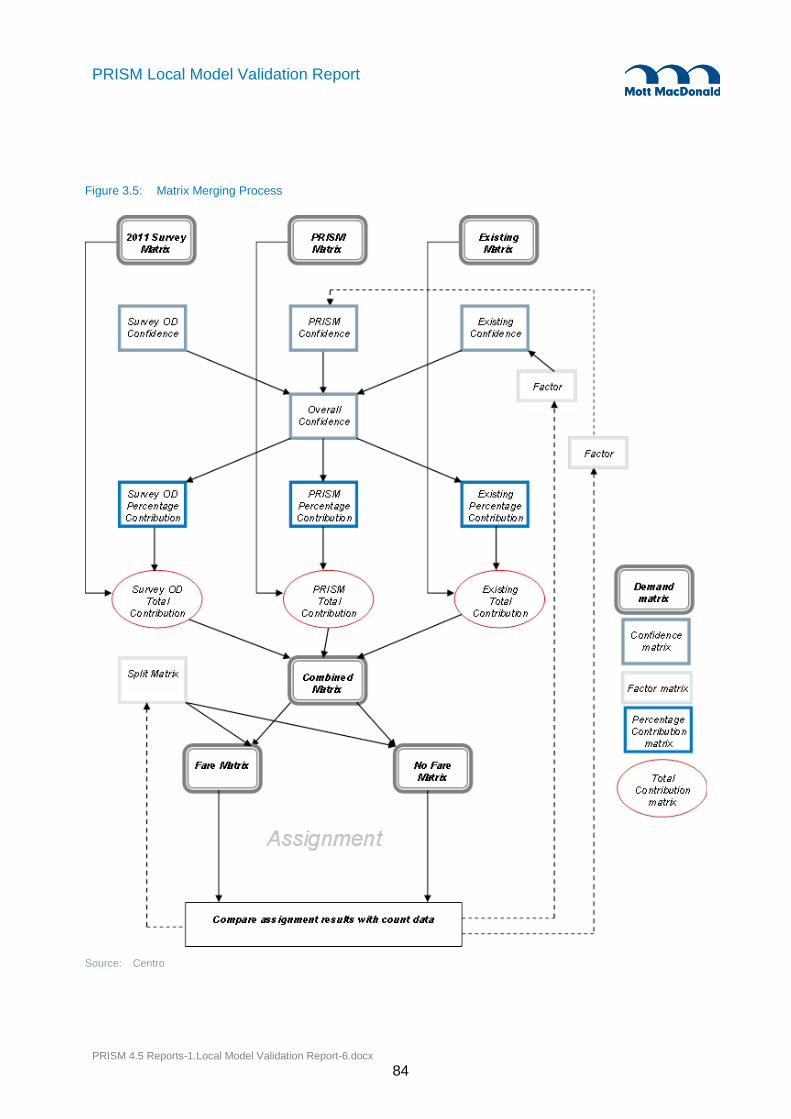
PRISM 4.5 Reports-1.Local Model Validation Report-6.docx
84
PRISM Local Model Validation Report
Figure 3.5: Matrix Merging Process
Source: Centro
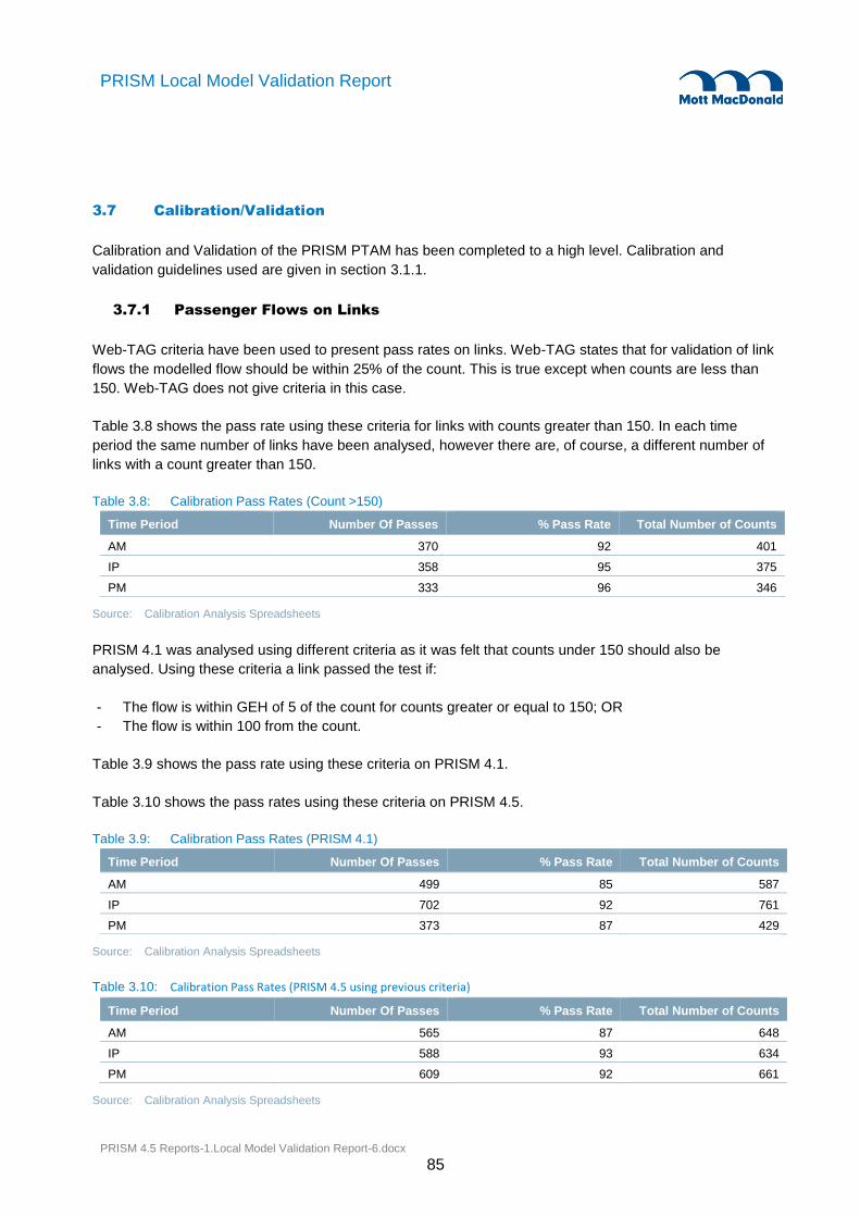
PRISM 4.5 Reports-1.Local Model Validation Report-6.docx
85
PRISM Local Model Validation Report
3.7 Calibration/Validation
Calibration and Validation of the PRISM PTAM has been completed to a high level. Calibration and
validation guidelines used are given in section 3.1.1.
3.7.1 Passenger Flows on Links
Web-TAG criteria have been used to present pass rates on links. Web-TAG states that for validation of link
flows the modelled flow should be within 25% of the count. This is true except when counts are less than
150. Web-TAG does not give criteria in this case.
Table 3.8 shows the pass rate using these criteria for links with counts greater than 150. In each time
period the same number of links have been analysed, however there are, of course, a different number of
links with a count greater than 150.
Table 3.8: Calibration Pass Rates (Count >150)
Time Period Number Of Passes % Pass Rate Total Number of Counts
AM 370 92 401
IP 358 95 375
PM 333 96 346
Source: Calibration Analysis Spreadsheets
PRISM 4.1 was analysed using different criteria as it was felt that counts under 150 should also be
analysed. Using these criteria a link passed the test if:
- The flow is within GEH of 5 of the count for counts greater or equal to 150; OR
- The flow is within 100 from the count.
Table 3.9 shows the pass rate using these criteria on PRISM 4.1.
Table 3.10 shows the pass rates using these criteria on PRISM 4.5.
Table 3.9: Calibration Pass Rates (PRISM 4.1)
Time Period Number Of Passes % Pass Rate Total Number of Counts
AM 499 85 587
IP 702 92 761
PM 373 87 429
Source: Calibration Analysis Spreadsheets
Table 3.10: Calibration Pass Rates (PRISM 4.5 using previous criteria)
Time Period Number Of Passes % Pass Rate Total Number of Counts
AM 565 87 648
IP 588 93 634
PM 609 92 661
Source: Calibration Analysis Spreadsheets

PRISM 4.5 Reports-1.Local Model Validation Report-6.docx
86
PRISM Local Model Validation Report
3.7.2 Passenger Usage at Stops
Passenger usage at stops refers to the boarding and alighting outputs produced by the model. The PLD
matrices have not been calibrated using boarding and alighting counts.
Web-TAG doesn’t give criteria for boarding and alighting counts. However the link criteria have been
adjusted so that counts under 50 are treated separately. Stops with a count under 50 must have the flow
within 12.5 of the count. This number is chosen as 12.5 is 25% of 50.
Table 3.11: Calibration Pass Rates (Boarding at Stops >50)
Time Period Number Of Passes % Pass Rate Total Number of Counts
IP 62 83 74
PM 66 81 81
AM 51 80 63
Source: Calibration Analysis Spreadsheets
Table 3.12: Calibration Pass Rates (Boarding at Stops for all counts)
Time Period Number Of Passes % Pass Rate Total Number of Counts
AM 98 70 139
IP 96 72 132
PM 106 72 146
Source: Calibration Analysis Spreadsheets
Table 3.13: Calibration Pass Rates (Alighting at Stops >50)
Time Period Number Of Passes % Pass Rate Total Number of Counts
AM 61 79 77
IP 57 73 78
PM 67 81 82
Source: Calibration Analysis Spreadsheets
Table 3.14: Calibration Pass Rates (Alighting at Stops for all counts)
Time Period Number Of Passes % Pass Rate Total Number of Counts
AM 103 74 139
IP 91 68 132
PM 113 77 146
Source: Calibration Analysis Spreadsheets
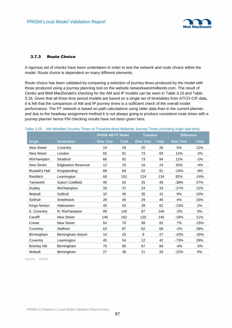
PRISM 4.5 Reports-1.Local Model Validation Report-6.docx
87
PRISM Local Model Validation Report
3.7.3 Route Choice
A rigorous set of checks have been undertaken in order to test the network and route choice within the
model. Route choice is dependent on many different elements.
Route choice has been validated by comparing a selection of journey times produced by the model with
those produced using a journey planning tool on the website networkwestmidlands.com. The result of
Centro and Mott MacDonald’s checking for the AM and IP models can be seen in Table 3.15 and Table
3.16. Given that all three time period models are based on a single set of timetables from ATCO-CIF data,
it is felt that the comparison of AM and IP journey times is a sufficient check of the overall model
performance. The PT network is based on path calculations using older data than in the current planner,
and due to the headway assignment method it is not always going to produce consistent route times with a
journey planner hence PM checking results have not been given here.
Table 3.15: AM Modelled Journey Times vs Traveline West Midlands Journey Times (including origin wait time)
PRISM AM PT Model Traveline Difference
Origin Destination Ride Time Total Ride Time Total Ride Time Total
New Street Coventry 19 29 20 26 5% 12%
New Street London 65 81 73 83 12% -2%
Wol’hampton Stratford 66 92 73 94 11% -2%
New Street Edgbaston Reservoir 12 23 16 24 33% -4%
Russell’s Hall Kingstanding 68 84 52 91 -24% -8%
Redditch Leamington 68 102 124 134 82% -24%
Tamworth Sutton Coldfield 40 62 25 49 -38% 27%
Dudley Wol’hampton 33 37 24 33 -27% 12%
Walsall Solihull 32 45 35 41 9% 10%
Solihull Smethwick 28 46 29 40 4% 15%
Kings Norton Halesowen 45 63 39 62 -13% 2%
E. Coventry N. Wol’hampton 89 140 87 140 -2% 0%
Cardiff New Street 146 162 120 146 -18% 11%
Crewe New Street 54 70 58 82 7% -15%
Coventry Stafford 63 87 62 68 -2% 28%
Birmingham Birmingham Airport 10 20 9 27 -10% -26%
Coventry Leamington 45 54 12 42 -73% 29%
Brierley Hill Birmingham 70 80 67 84 -4% -5%
Walsall Birmingham 27 36 21 33 -22% 9%
Source: Centro

PRISM 4.5 Reports-1.Local Model Validation Report-6.docx
88
PRISM Local Model Validation Report
Table 3.16: IP Modelled Journey Times vs Traveline West Midlands Journey Times (excluding origin wait time)
PRISM IP PT Model Traveline Difference
Origin Destination Ride Time Total Ride Time Total Ride Time Total
New Street Coventry 18 28 20 23 11% -18%
New Street London 72 88 84 84 17% -5%
Wol’hampton Stratford 65 91 80 96 23% 5%
Redditch Leamington 62 98 62 112 0% 14%
Tamworth Sutton Coldfield 40 62 19 49 -53% -21%
Dudley Wol’hamtpon 33 37 25 34 -24% -8%
Walsall Solihull 32 39 38 41 19% 5%
Kings Norton Halesowen 45 58 37 59 -18% 2%
East Coventry N. Wol’hampton 85 135 91 141 7% 4%
New Street Coventry 18 28 20 23 11% -18%
Source: Mott MacDonald
3.7.4 Cordons and All-Mode Counts
The overall calibration shows an excellent fit between model and counts for both link flows and passenger
boarding and alighting’s, The above tables show that over 85% of link flows passed the WebTAG criteria in
over 85% of cases, and that boarding/alighting results are good although not quite to WebTAG levels. This
is a satisfactory level of calibration for a model of this size.
Further analysis of the trip matrix has been conducted at a more spatially detailed level. The table below
presents the link calibration results at LTP cordon and district cordon (bus), and separately for rail and
Metro.
Table 3.17: Link Calibration Results at LTP Cordon, District Cordon (Bus only), All-Rail and All-Metro Levels
Cordon/Mode
AM IP PM
Total Sites % Sites Pass Total Sites % Sites Pass Total Sites Sites Pass
LTP Cordons 135 93% 141 94% 152 95%
District Cordons 103 92% 118 97% 69 93%
All-Rail counts 80 89% 33 94% 82 96%
All-Metro counts 44 100% 44 100% 44 100%
P&R counts 61 70% 61 88% 61 93%
Source: Mott MacDonald
As seen in Appendix F, when the overall model statistics are broken down there are areas which perform
above the pass criteria, and those which fall below. Overall the model is considered to be of a high quality
in terms of calibration.
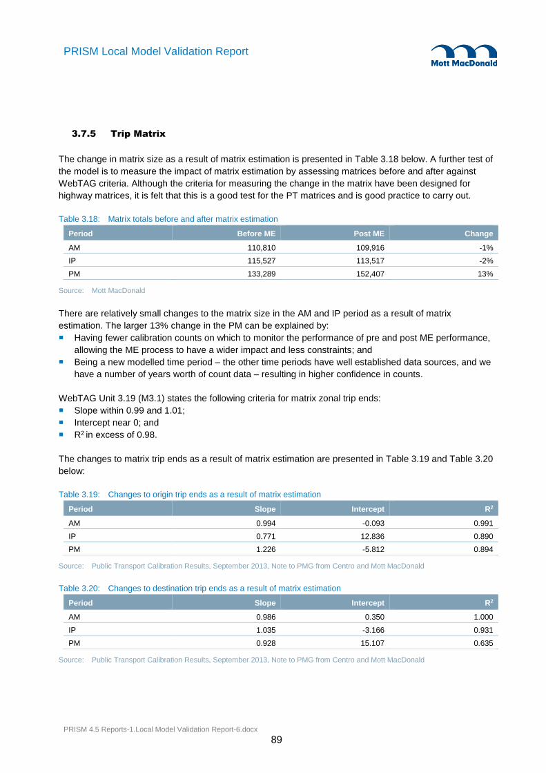
PRISM 4.5 Reports-1.Local Model Validation Report-6.docx
89
PRISM Local Model Validation Report
3.7.5 Trip Matrix
The change in matrix size as a result of matrix estimation is presented in Table 3.18 below. A further test of
the model is to measure the impact of matrix estimation by assessing matrices before and after against
WebTAG criteria. Although the criteria for measuring the change in the matrix have been designed for
highway matrices, it is felt that this is a good test for the PT matrices and is good practice to carry out.
Table 3.18: Matrix totals before and after matrix estimation
Period Before ME Post ME Change
AM 110,810 109,916 -1%
IP 115,527 113,517 -2%
PM 133,289 152,407 13%
Source: Mott MacDonald
There are relatively small changes to the matrix size in the AM and IP period as a result of matrix
estimation. The larger 13% change in the PM can be explained by:
Having fewer calibration counts on which to monitor the performance of pre and post ME performance,
allowing the ME process to have a wider impact and less constraints; and
Being a new modelled time period – the other time periods have well established data sources, and we
have a number of years worth of count data – resulting in higher confidence in counts.
WebTAG Unit 3.19 (M3.1) states the following criteria for matrix zonal trip ends:
Slope within 0.99 and 1.01;
Intercept near 0; and
R2 in excess of 0.98.
The changes to matrix trip ends as a result of matrix estimation are presented in Table 3.19 and Table 3.20
below:
Table 3.19: Changes to origin trip ends as a result of matrix estimation
Period Slope Intercept R2
AM 0.994 -0.093 0.991
IP 0.771 12.836 0.890
PM 1.226 -5.812 0.894
Source: Public Transport Calibration Results, September 2013, Note to PMG from Centro and Mott MacDonald
Table 3.20: Changes to destination trip ends as a result of matrix estimation
Period Slope Intercept R2
AM 0.986 0.350 1.000
IP 1.035 -3.166 0.931
PM 0.928 15.107 0.635
Source: Public Transport Calibration Results, September 2013, Note to PMG from Centro and Mott MacDonald

PRISM 4.5 Reports-1.Local Model Validation Report-6.docx
90
PRISM Local Model Validation Report
TAG Unit 3.19 (M3.1) states the following values for zonal cell values:
Slope within 0.98 and 1.02;
Intercept near 0; and
R2 in excess of 0.95.
The results of the zonal test are presented in Table 3.21.
Table 3.21: Changes to origin—destination pairs as a result of matrix estimation
Period Slope Intercept R2
AM 0.993 0.000 0.994
IP 0.730 0.008 0.667
PM 0.933 0.008 0.535
Source: Public Transport Calibration Results, September 2013, Note to PMG from Centro and Mott MacDonald
As expected there are bigger changes applied to the PM matrices. Given that this is a new modelled time
period, the matrix change statistics suggest that this can be improved in subsequent model enhancements.
This test is not a guideline for PT matrices in WebTAG; however it was felt it was good practice to carry out
the analysis, to demonstrate that the impact of matrix estimation is not significantly impacting on the
structure of the matrices.
It is good practice to compare trip length distributions both in terms of before and after matrix estimation,
and where possible against independent data. For the PT model both comparisons have been done for all
time periods, using National Travel Survey (NTS) data (as provided by the HA) as the independent trip
length data.
The NTS data is already packaged in to trip length bands, with model outputs calculated to match so that
direct comparisons can be made. Due to sample size limitations the NTS data has been aggregated to all
day, for trips which have a trip end in the West Midlands. There are particularly small samples of rail data,
which is exaggerated in the IP period, meaning that splitting the data by time period would introduce bias.
As can be seen in Figure 3.6:
Overall there is a good fit across all time periods to the NTS distribution, with a general pattern of an
underestimate of short trips, and an over estimate of long trips; and
The impact of matrix estimation is relatively small for all time periods, which demonstrates in part that
the shape and structure of the matrices are only subject to small changes.

PRISM 4.5 Reports-1.Local Model Validation Report-6.docx
91
PRISM Local Model Validation Report
Figure 3.6: Public transport trip length distributions before and after matrix estimation and NTS
Source: Mott MacDonald
3.7.6 Independent Validation
Validation of the model uses counts and statistics independent of calibration to confirm that the model is
producing sensible outputs. The original specification included using the district cordon data for validation;
however in developing the matrices it was felt that this data would be better used in calibration.
The above trip length analysis is regarded as validation in terms of comparing modelled versus NTS
distribution, and in addition to this the model is validated in terms of:
Average bus wait time, access/egress time, journey time and number of interchanges compared to
Centro’s bus user profile; and
Select links on Midland Metro which were not included in matrix estimation.
Table 3.22 presents assigned bus trip leg assignment outputs compared to Centro’s Bus User Profile
(BUP). The BUP data is presented for all bus passengers interviewed; it is not possible to split this by time
period so it represents an overall average for comparison.

PRISM 4.5 Reports-1.Local Model Validation Report-6.docx
92
PRISM Local Model Validation Report
Table 3.22: Comparison of bus average journey times against Centro’s Bus User Profile
Trip element Bus User Profile AM IP PM
Walk access/egress time 07:07 09:17 08:20 09:17
Wait time 07:10 05:39 02:36 05:39
Journey time 23:10 23:44 20:14 23:44
Average number interchanges
1.2 0.7 0.6 0.7
Source: Public Transport Calibration Results, September 2013, Note to PMG from Centro and Mott MacDonald
The modelled results are calculated using the demand weighted averages from the bus skims and bus-sub
mode demand matrices, consequently bus trips made as part of a longer journey (i.e. accessing metro or
rail) are not included. . All of the bus user profile data is based on perceived rather than actual time. The
perceived walk access time is lower than those extracted from the model. This could be explained by the
fact that we are missing journeys accessing or egressing a train journey which will typically require a
shorter than average walk time between the station and bus stop. Likewise the number of interchanges
being small than average is likely due to the fact we are excluding those journeys that interchange from a
bus to another sub-mode.
A full set of passenger counts were available, in the form of boarding and alighting counts for all Midland
Metro stops. Selected counts were not used in calibration and retained for validation. The performance of
these links, comparing modelled versus counts, are presented in overleaf.
Table 3.23 shows a high level of fit between counts and modelled flows on Midland Metro in all time
periods. All individual counts are within the 15% criteria. Along with the calibration data presented above
this confirms that the assignment fit on Midland Metro is at a high level for both calibration and validation.
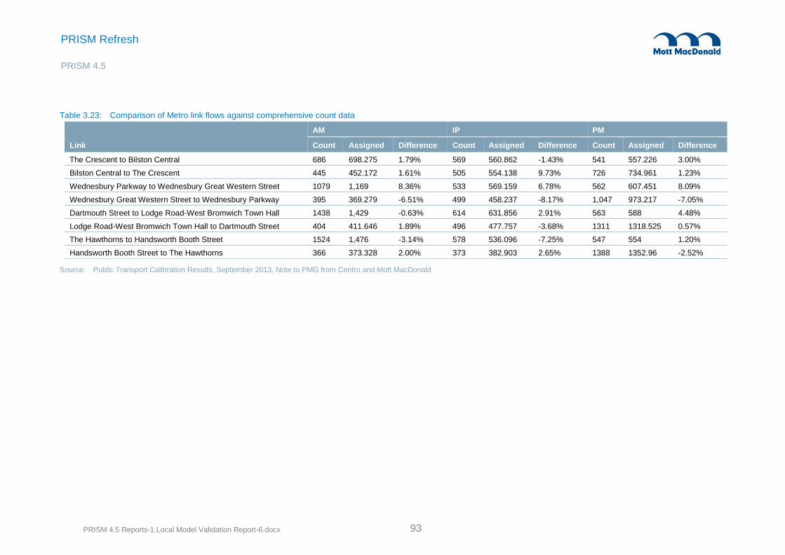
PRISM 4.5 Reports-1.Local Model Validation Report-6.docx 93
PRISM Refresh
PRISM 4.5
Table 3.23: Comparison of Metro link flows against comprehensive count data
Link
AM IP PM
Count Assigned Difference Count Assigned Difference Count Assigned Difference
The Crescent to Bilston Central 686 698.275 1.79% 569 560.862 -1.43% 541 557.226 3.00%
Bilston Central to The Crescent 445 452.172 1.61% 505 554.138 9.73% 726 734.961 1.23%
Wednesbury Parkway to Wednesbury Great Western Street 1079 1,169 8.36% 533 569.159 6.78% 562 607.451 8.09%
Wednesbury Great Western Street to Wednesbury Parkway 395 369.279 -6.51% 499 458.237 -8.17% 1,047 973.217 -7.05%
Dartmouth Street to Lodge Road-West Bromwich Town Hall 1438 1,429 -0.63% 614 631.856 2.91% 563 588 4.48%
Lodge Road-West Bromwich Town Hall to Dartmouth Street 404 411.646 1.89% 496 477.757 -3.68% 1311 1318.525 0.57%
The Hawthorns to Handsworth Booth Street 1524 1,476 -3.14% 578 536.096 -7.25% 547 554 1.20%
Handsworth Booth Street to The Hawthorns 366 373.328 2.00% 373 382.903 2.65% 1388 1352.96 -2.52%
Source: Public Transport Calibration Results, September 2013, Note to PMG from Centro and Mott MacDonald

PRISM 4.5 Reports-1.Local Model Validation Report-6.docx
94
PRISM Local Model Validation Report
PRISM 4.5
3.8 Summary
3.8.1 Model Development
The PRISM PTAM was built based roughly on two older models and was designed so that one network
could be used by both Mott MacDonald and Centro. The model is most detailed within the core area where
there are smaller zones and the link network is built from the OS OSCAR road network dataset. Outside of
the core area there is less detail and links exist as straight lines only between stops. The rail network is
more detailed outside of the core area than the bus network and rail links match the actual path of rail lines.
All data belonging to PT services including the service route and timetable information has been
downloaded from the NPTDR for 2011. Data from the NPTDR is in ATCO-CIF file format. This data has
been converted to Visum format by PTV during the beginning stages of the model development.
The model has been updated in various other ways. Firstly the fares included in the model have been
updated to a 2011 rate. A single boarding penalty is applied to all bus services whereas metro and train
services include a fixed boarding penalty plus a distance based fare. The PT matrices have been updated
using various sources from survey data to synthetic data produced by the PRISM demand model to
matrices from older PT models to PLD matrices. New count data has been collected from various sources
in order to calibrate the model.
3.8.2 Standards Achieved
The WebTAG guidance available for Public Transport modelling is not plentiful but it has been incorporated
where possible. The criteria defined in the WebTAG units have been used as a guide rather than a strict
set of targets. This is because the observed data available warranted a different approach. The criteria
defined by Centro and Mott MacDonald are similar to the WebTAG criteria but account for lower observed
counts.
The model meets these targets well and the results are consistent across time periods and different modes
of transport and the calibration and validation for metro is particularly creditable. The quality of the trip
matrix has not been compromised to meet the guideline validation criteria.
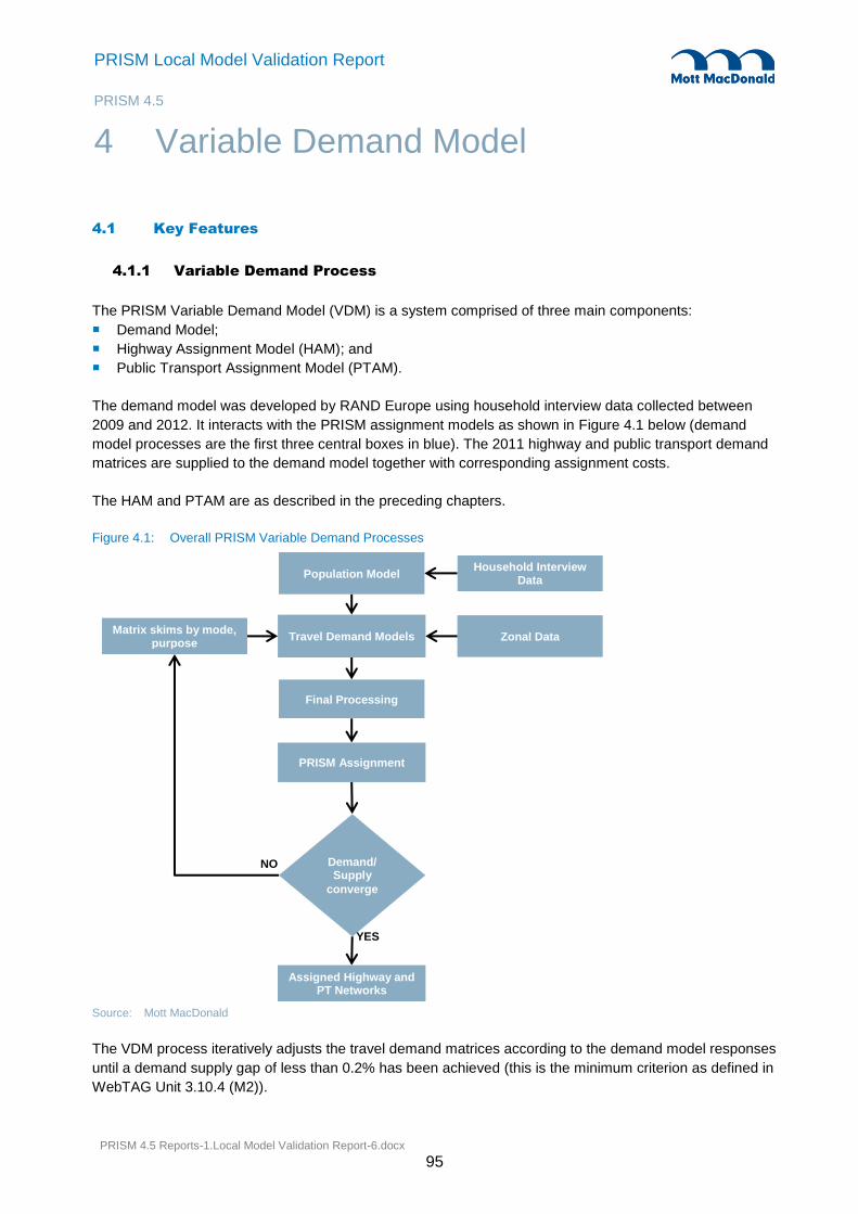
PRISM 4.5 Reports-1.Local Model Validation Report-6.docx
95
PRISM Local Model Validation Report
PRISM 4.5
4.1 Key Features
4.1.1 Variable Demand Process
The PRISM Variable Demand Model (VDM) is a system comprised of three main components:
Demand Model;
Highway Assignment Model (HAM); and
Public Transport Assignment Model (PTAM).
The demand model was developed by RAND Europe using household interview data collected between
2009 and 2012. It interacts with the PRISM assignment models as shown in Figure 4.1 below (demand
model processes are the first three central boxes in blue). The 2011 highway and public transport demand
matrices are supplied to the demand model together with corresponding assignment costs.
The HAM and PTAM are as described in the preceding chapters.
Figure 4.1: Overall PRISM Variable Demand Processes
Source: Mott MacDonald
The VDM process iteratively adjusts the travel demand matrices according to the demand model responses
until a demand supply gap of less than 0.2% has been achieved (this is the minimum criterion as defined in
WebTAG Unit 3.10.4 (M2)).
4 Variable Demand Model
Population Model Household Interview
Data
Assigned Highway and PT Networks
Matrix skims by mode, purpose
Zonal Data
Final Processing
Travel Demand Models
PRISM Assignment
Demand/Supply
converge
YES
NO

PRISM 4.5 Reports-1.Local Model Validation Report-6.docx
96
PRISM Local Model Validation Report
PRISM 4.5
4.2 Demand Model
An overview of the Demand model and its key features is made available in the following section, however
for fuller descriptions please see the reports by RAND:12
PRISM 2011 Base: Mode-Destination Model Estimation
PRISM 2011 Base: Frequency and Car Ownership Models
PRISM 2011 Base: Demand Model Implementation.
4.2.1 Overview
The demand model consists of the following three main components:
1. The Population Model. This contains a prototypical sampling procedure and a car ownership model
that produce projections of the future West Midlands population that are not influenced by accessibility.
The population segmentation adopted is as described further below;
2. The Travel Demand Model. This calculates travel accessibility and applies frequency, mode choice,
destination choice, PT access mode, Park & Ride station choice, and time period choice – the variable
demand responses. Essentially this component predicts the future travel choices of the West Midlands
population projected by the Population Model; and
3. The Final Processing Model takes the predicted trip matrices for each mode, purpose and time period,
sums these matrices over travel purposes to reflect the more aggregate segmentations represented in
the assignments, and then applies a pivoting procedure to predict changes in demand relative to the
base matrices.
The outcome of these three processes is a set of revised demand matrices for assignment in the HAM and
PTAM. These new matrices include responses to cost changes in the assignment model. An important
consideration is that the PTAM is not demand-constrained meaning that, unlike the HAM, the assignment
costs do not change when the demand matrices change. It is for this reason that the PTAM is a fixed input
to the VDM process rather than being part of the so-called VDM-loop.
4.2.1.1 Purpose Segmentation
The demand model uses population segments that define the key social-economic effects that are
represented in the frequency and mode destination models including car availability and income. The
demand to travel for each of these population segments is applied separately for the various purpose
segments in the PRISM Demand Model, as shown in Table 4.1.
12 All 3 Rand reports are available on the PRISM website http://www.prism-wm.com/ and from the RAND website at the following links
http://www.rand.org/pubs/research_reports/RR186.html
http://www.rand.org/pubs/research_reports/RR273.html
http://www.rand.org/pubs/research_reports/RR314.html

PRISM 4.5 Reports-1.Local Model Validation Report-6.docx
97
PRISM Local Model Validation Report
PRISM 4.5
Table 4.1: Demand model purpose segmentation
Home Based Non-home based
HB Work (commuting) NHB work-work tours
HB Business NHB work-other tours
HB Primary education NHB other-other tours
HB Secondary education NHB work-work detours
HB Tertiary education NHB work-other detours
HB Shopping NHB other-other detours
HB Escort
HB Other
Source: Mott MacDonald
4.2.1.2 The Population Model
The Population Model uses the 2009-2012 West Midlands household interview samples and zonal targets
to generate zonal population segments by purpose which are then supplied to the Travel Demand Model.
Essentially the Population Model has three sub-processes:
a) Prototype sampling. This expands the base household interview (HI) sample to meet zonal
population targets that are defined for each PRISM zone in the FMA. The base HI data has been
drawn from 5,030 interviews collected in 2009-2012 and contains enough person and household
information to define all the required socio-economic segmentation;
b) Car ownership modelling. This calculates the car ownership probabilities for each household in the
prototypical sample. The complete car ownership model predicts the probability that a household owns
zero, one, two and three-plus cars using household income, household licence holding, number of
workers, number of infants and children and head of household gender, age and ethnicity. The car
ownership model then expands these predictions to the predicted number of households in each zone;
and
c) Zone segment accumulation. The outputs from the prototypical sampling procedure and the car
ownership model are combined and the forecast population is accumulated over the social-economic
segmentations represented in the travel demand models. This gives zonal segments by purpose.
Figure 4.2: Population Model
Source: Mott MacDonald
Base Person and Household Samples
Zonal Segment Accumulation
Zonal Targets Car Ownership Model
Zonal Segments by Purpose
Prototypical Sampling

PRISM 4.5 Reports-1.Local Model Validation Report-6.docx
98
PRISM Local Model Validation Report
PRISM 4.5
Validation of the prototype sampling, car ownership modelling and zone segmentation accumulation are
summarised in Section 4.3.3 and 4.3.4 and demonstrates that the variable demand model has been
constructed to fit well with the datasets used and is consistent with NTEM forecasts. The demand model
response parameters for frequency, distribution and mode choice have been estimated from West
Midlands data. The relative sensitivity of mode and destination choices is consistent with WebTAG
guidance, and the model elasticities and implied values-of-time have also been validated against WebTAG
values. The validation undertaken during estimation of the mode-destination is validated in Chapter 6 of the
mode-destination estimation report.13
4.2.1.3 The Travel Demand Model
The Travel Demand Model calculates total travel demand by applying tour frequencies to zonal populations
by segment and purpose that are produced by the Population Model. These are then distributed over the
available modes, destinations and any other alternatives represented. The full process is shown in Figure
4.3 below.
The Travel Demand Model uses the following intervals for time period choice:
AM-peak; 0700-0930hrs
Inter-Peak; 0930-1530hrs
PM-Peak; 1530-1900hrs
Off-Peak; 1900-0700hrs (demand model only).
For destination choice the process includes all PRISM model zones that cover core, intermediate and
external areas. The Travel Demand Model only considers destination alternatives where a non-zero
attraction variable is defined for the destination. Attraction variables are defined as the planning data
variables used by the Travel Demand Model. They are explained in more detail in section 4.3.1.
13 PRISM 2011 Mode-Destination Model Estimation, J Fox, B Patruni, A Daly, S Patil (http://www.rand.org/pubs/research_reports/RR186.html)

PRISM 4.5 Reports-1.Local Model Validation Report-6.docx
99
PRISM Local Model Validation Report
PRISM 4.5
Figure 4.3: Travel Demand Models
Source: Mott MacDonald
For mode choice the following seven main modes are modelled:
Car driver;
Car passenger;
Train;
Metro;
Bus;
Cycle; and
Walk.
In Figure 4.3, Zone Segments by Purpose are generated by the Population Model and are provided as
separate files for each HB travel purpose. Each file gives the number of persons in each model zone for
each of the travel segments relevant for that travel purpose. Zone Data consists of attraction variables and
parking cost data (for each zone) and describes the attractiveness of destinations. Highway & PT Skims
include travel time costs, toll costs and distance costs from the HAM as well as level-of-service skims from
the PTAM. The output from the Travel Demand Model consists of tour legs by purpose, mode and time
period that are in Production-Attraction format.
The tables below (Table 4.2 to Table 4.7) show an overview of the model structure for each of the purposes
of the travel demand model. Choices at the highest level in the structure are least sensitive to changes in
utility (Highway and PT cost skims), and then the sensitivity increases working down to the lowest and most
sensitive choice. In the tables presented below, the sensitivities are presented relative to the highest level
Distribution over modes,
Destination and Stations
Zonal Data
(Attraction Variables & Parking Cost Data)
Tour Frequency
Zonal Segments by Purpose
Log sums by Segment
Tour legs by Purpose and Mode
Highway & PT Cost
Skims

PRISM 4.5 Reports-1.Local Model Validation Report-6.docx
100
PRISM Local Model Validation Report
PRISM 4.5
choice, which is main mode choice for all of the models (the least sensitive choice). The tables present the
structural parameters which indicate the sensitivity of the choices relative to main mode choice. If the
structural parameter for adjacent choices is constrained to a value of one, this means that the choices are
effectively at the same level in the choice hierarchy and are equally sensitive to changes in utility (a
multinomial structure).
Table 4.2: Final model structure, commute and home-shopping
Choice Commuting Home-shopping
main mode choice
car driver time period choice 1.00 1.00
train & metro access mode choice 1.00 1.00
destination choice 0.78 0.42
train & metro station choice 0.33 0.40
Source: PRISM 2011 Base: Mode-Destination Model Estimation, Table 73, RAND Europe,
http://www.rand.org/pubs/research_reports/RR186.html
Table 4.3: Final model structure, home-other travel
Choice Home-other travel
main mode choice
car driver time period choice 1.00
train & metro access mode choice 1.00
train & metro station choice 0.43
destination choice 0.27
Source: PRISM 2011 Base: Mode-Destination Model Estimation, Table 74, RAND Europe,
http://www.rand.org/pubs/research_reports/RR186.html
Table 4.4: Final model structures, home–business and home–escort
Choice Home-business Home-escort
main mode choice
car driver time period choice 1.00 1.00
destination choice 0.19 0.47
Source: PRISM 2011 Base: Mode-Destination Model Estimation, Table 75, RAND Europe,
http://www.rand.org/pubs/research_reports/RR186.html
Table 4.5: Final model structures, home–education purposes
Choice Home-primary education
Home-secondary education
Home-tertiary education
main mode choice
destination choice 1.00 0.58 0.69
Source: PRISM 2011 Base: Mode-Destination Model Estimation, Table 76, RAND Europe,
http://www.rand.org/pubs/research_reports/RR186.html

PRISM 4.5 Reports-1.Local Model Validation Report-6.docx
101
PRISM Local Model Validation Report
PRISM 4.5
Table 4.6: Final model structures, PD-based tour models
Choice Work-related PD to work-related SD
Work-related PD to other SD
Other PD to other SD
main mode choice
destination choice 1.00 1.00 1.00
Source: PRISM 2011 Base: Mode-Destination Model Estimation, Table 77, RAND Europe,
http://www.rand.org/pubs/research_reports/RR186.html
Table 4.7: Final model structures, detour models
Choice Work-related PD to work-related SD
Work-related PD to other SD
Other PD to other SD
main mode choice
destination choice 1.00 1.00 0.25
Source: PRISM 2011 Base: Mode-Destination Model Estimation, Table 78, RAND Europe,
http://www.rand.org/pubs/research_reports/RR186.html
Detailed descriptions of the calculation of log sums, tour frequency and distribution over modes, destination
and stations can be found in the Demand Model Implementation report14 and Mode-Destination Model
Estimation Report.15 It suffices here to indicate that the calculated log sums are used to compute the choice
probabilities across levels of the nesting structure for the demand model. Tour frequencies give the
probability of trip making. The demand predicted by the frequency model is then distributed over available
main modes, time periods and destinations. This produces the PA tour matrices that are used in the Final
Processing Model.
The travel demand models are singly constrained for all purposes. As the models are applied using a
pivoting procedure to define changes relative to the base matrices, and the base matrices are effectively
double-constrained, then standard RAND Europe practice is to work with single-constrained mode-
destination choice models.
4.2.1.4 The Final Processing Model
As a last main stage of the VDM processes, the Final Processing Model transposes the calculated PA-
based tour legs to create an OD matrix by transposing and adding relevant home-based purposes. This is
then followed by a simple pivoting process.
Essentially, for the eight HB purposes, matrices of outward and return tour legs are output split by the four
model time periods. Outward tour leg matrices, which represent travel from the home to primary
destinations, are equivalent to trip matrices and so are used directly. However return tour leg matrices,
need to be transposed before they can be treated as trip matrices. ALOGIT code is used to transpose the
matrices. The next step is to add up the matrices across purposes to reflect the segmentations used in the
Visum assignments.
14 PRISM 2011 Base Demand Model Implementation, J Fox, B Patruni, A Daly (http://www.rand.org/pubs/research_reports/RR314.html)
15 PRISM 2011 Mode-Destination Model Estimation, J Fox, B Patruni, A Daly, S Patil (http://www.rand.org/pubs/research_reports/RR186.html)
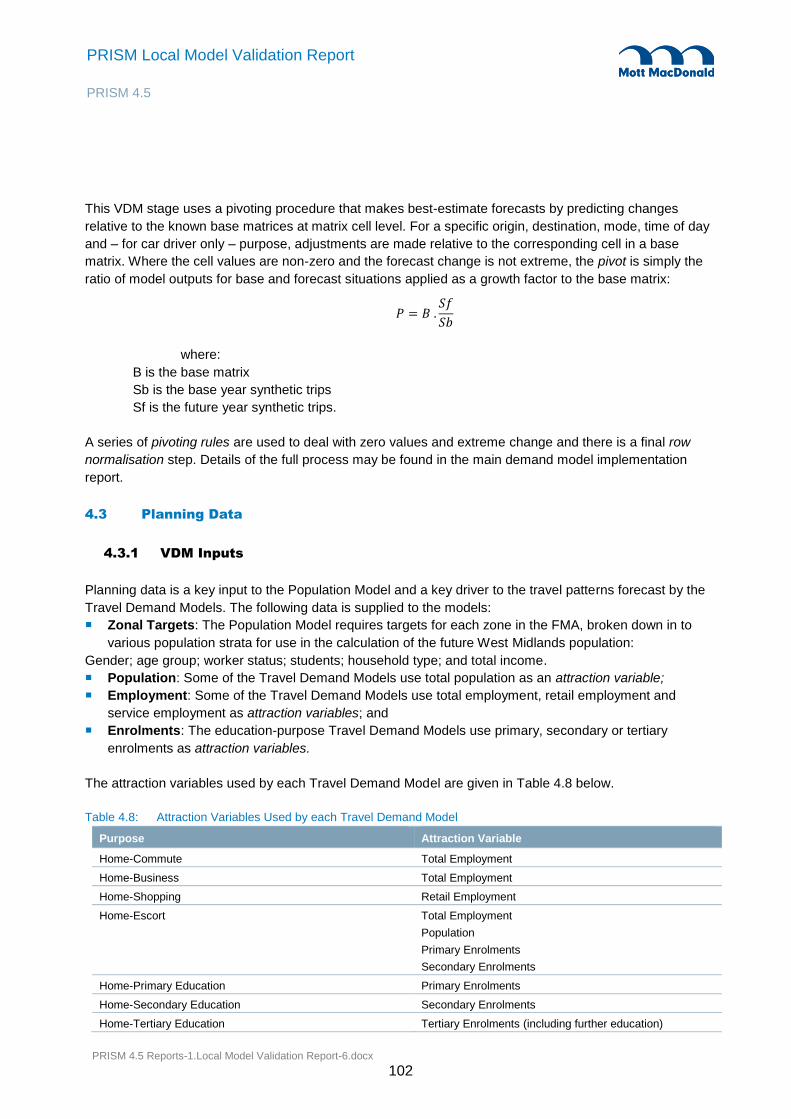
PRISM 4.5 Reports-1.Local Model Validation Report-6.docx
102
PRISM Local Model Validation Report
PRISM 4.5
This VDM stage uses a pivoting procedure that makes best-estimate forecasts by predicting changes
relative to the known base matrices at matrix cell level. For a specific origin, destination, mode, time of day
and – for car driver only – purpose, adjustments are made relative to the corresponding cell in a base
matrix. Where the cell values are non-zero and the forecast change is not extreme, the pivot is simply the
ratio of model outputs for base and forecast situations applied as a growth factor to the base matrix:
𝑃 = 𝐵 .𝑆𝑓
𝑆𝑏
where:
B is the base matrix
Sb is the base year synthetic trips
Sf is the future year synthetic trips.
A series of pivoting rules are used to deal with zero values and extreme change and there is a final row
normalisation step. Details of the full process may be found in the main demand model implementation
report.
4.3 Planning Data
4.3.1 VDM Inputs
Planning data is a key input to the Population Model and a key driver to the travel patterns forecast by the
Travel Demand Models. The following data is supplied to the models:
Zonal Targets: The Population Model requires targets for each zone in the FMA, broken down in to
various population strata for use in the calculation of the future West Midlands population:
Gender; age group; worker status; students; household type; and total income.
Population: Some of the Travel Demand Models use total population as an attraction variable;
Employment: Some of the Travel Demand Models use total employment, retail employment and
service employment as attraction variables; and
Enrolments: The education-purpose Travel Demand Models use primary, secondary or tertiary
enrolments as attraction variables.
The attraction variables used by each Travel Demand Model are given in Table 4.8 below.
Table 4.8: Attraction Variables Used by each Travel Demand Model
Purpose Attraction Variable
Home-Commute Total Employment
Home-Business Total Employment
Home-Shopping Retail Employment
Home-Escort Total Employment
Population
Primary Enrolments
Secondary Enrolments
Home-Primary Education Primary Enrolments
Home-Secondary Education Secondary Enrolments
Home-Tertiary Education Tertiary Enrolments (including further education)

PRISM 4.5 Reports-1.Local Model Validation Report-6.docx
103
PRISM Local Model Validation Report
PRISM 4.5
Purpose Attraction Variable
Total Employment
Home-Other Population
Service Employment
Retail Employment
Source: PRISM 2011 Base: Demand Model Implementation, Table 54, RAND Europe,
http://www.rand.org/content/dam/rand/pubs/research_reports/RR300/RR314/RAND_RR314.pdf
4.3.2 Data Sources and Key Assumptions
4.3.2.1 Population
2011 population figures for PRISM zones in the AoDM were calculated from Census data for Output Areas
(OAs) by apportioning based on residential Address Points (APs). Outside of the AoDM, the OA
populations were attributed to the zone containing the OA centroids. All figures were then constrained to
2011 NTEM district totals to be consistent with WebTAG guidance.
The 2011 population figures can be found in Appendix I.
4.3.2.2 Employment
Data from the Inter-Departmental Business Register (IDBR) was used to calculate the number of jobs
within each PRISM zone in the PRISM AoDM. This was taken from an IDBR file sourced via Solihull for use
with the PRISM model only. Following checks on the IDBR source data, a number of changes were made
to the file to amend records identified as being inaccurate. These figures were then constrained to 2011
NTEM 6.2 district totals to be consistent with WebTAG guidance.
Outside of the AoDM, Lower-Super Output Area (LSOA) Business Register and Employment Survey
(BRES) figures were used to calculate an initial number of jobs before being constrained to 2011 NTEM 6.2
district totals to be consistent with WebTAG guidance.
There were some areas where LSOAs overlapped multiple PRISM zones. A number of alternatives were
explored including using proportional overlap to apportion these zones. However this was found to
introduce a number of significant errors and it was decided that using LSOA centroids was the best
method. Detailed checks outlined one significant issue where the zone containing Coventry airport had all
the jobs assigned to its neighbouring zone due to the location of the LSOA centroid. Manual adjustments
were made using the modellers judgement, assigning 10% of jobs in zone 8576 and 90% to 8598 where
the airport is located.
The 2011 employment figures can be found in Appendix J.

PRISM 4.5 Reports-1.Local Model Validation Report-6.docx
104
PRISM Local Model Validation Report
PRISM 4.5
4.3.2.3 Enrolments
2011 enrolments were derived from four key sources:
Department for Education Source 1: “DfE: Schools, Pupils and their Characteristics, January 2011” –
The statistical first release (SFR) based on the 2011 School Census;
Edubase: Data from the Department for Education downloaded in June 2012;
Higher Education Statistics Agency Source 1: “Table 1 - All students by HE institution, level of
study, mode of study and domicile 2010/11”; and
Department for Education Source 2: “Performance tables 2010: Key Stage 5”.
Data from the first Department for Education source (above) was combined with the Edubase source. The
majority of schools appear in both lists but duplicates were removed. Any schools which opened from 1st
September 2011 were not included and schools which have closed since this date were retained.
Enrolments data is used PRISM as the attraction variable for home-based primary education and escort
tours. Attraction variables affect the distribution of tours over alternatives rather than the number of tours
generated.
Nursery school pupils are excluded from the PRISM enrolments data because they do not fit in to the
categories of primary, secondary or tertiary education. Most nursery establishments were removed based
on the ‘type’ of the establishment. Where the ‘type’ of establishment was unavailable the following
assumptions were made:
If >80% of pupils were aged 0-3, ALL pupils were considered to be of nursery school age;
If >80% of pupils were aged 4-10, ALL pupils were considered to be of primary school age; and
If >80% of pupils were aged 11+, ALL pupils were considered to be of secondary school or further
education age.
If less than 80% of pupils were any particular age category, the total number of pupils was split
proportionally by the number of pupils in each age category.
Other assumptions:
Further education students were separated from secondary school pupils based on age;
In the small proportion of cases where pupil or student numbers were unknown, capacities were
assumed to equal pupil numbers; and
Websites for establishments with the word ‘college’ or university in their names were checked to see if
they have more than one campus. A comparison to Ordnance Survey 1:25,000 maps identified some
other campuses but the majority of schools shown on Ordnance Survey maps but missing from the list
had closed in recent years.
The 2011 enrolments figures can be found in Appendix K.
4.3.2.4 Zonal Targets
The Population Model requires population targets for each zone in the AoDM. These targets are broken
down in to various population strata for use in the calculation of the future West Midlands population. At the
time the model was developed, the only information available at the required level of detail came from the
2001 Census and this was the starting point for developing the 2011 Zonal Targets.

PRISM 4.5 Reports-1.Local Model Validation Report-6.docx
105
PRISM Local Model Validation Report
PRISM 4.5
To be precise, the zonal targets from the original PRISM model were used as the starting point. The data
required re-zoning (to the new PRISM zoning system) before being adjusted to match the population totals
for each zone that was available from the 2011 Census. The following information for each zone was
therefore retained from the 2001 Census:
Gender proportions;
Age group proportions;
Household-type proportions;
Worker status proportions;
Worker-to-population ratio;
Student-to-population ratio; and
Household-to-population ratio.
An important zonal target that was not used in the original PRISM model is total household income. The
following approach was used for estimating the total household income for each zone in the AoDM:
4. Take CACI household income data from 2004/5 (available from PRISM v2); and
5. Apply real increase in household income from 2004/5 to 2011 of 1.2%.16
The 2011 zonal target figures can be found in Appendix L.
4.3.3 Demand Model Validation
Various validation tests are made with the Demand Model which essentially consist of running the model
for 2011 and comparing the outputs against observations in the 2009-2012 household interview surveys.
4.3.3.1 Population Model Validation
Three validation tests of the Population Model are presented here:
Overall fit to zonal targets;
Car ownership validation; and
Population distribution validation.
Overall Fit to Zonal Targets
The prototype sampling step of the Population Model expands the 2011 HI sample to meet zonal
population targets. This validation test looks at how well the prototypical sampling step has performed to
reach the overall zonal targets, as shown in Table 4.9 below.
Table 4.9: Prototypical sample expansion compared to zonal targets
Population Segment Target Total Predicted Total % diff.
males 2,116,559 2,133,750 0.8%
females 2,180,139 2,154,473 -1.2%
aged 0–20 1,091,867 1,135,038 4%
aged 21–44 1,452,310 1,484,962 2.2%
aged 45–64 1,054,830 1,024,633 -2.9%
16 Office National Statistics, UKEA and Blue Book; World Database of Happiness

PRISM 4.5 Reports-1.Local Model Validation Report-6.docx
106
PRISM Local Model Validation Report
PRISM 4.5
Population Segment Target Total Predicted Total % diff.
aged 65+ 697,706 643,471 -7.8%
full-time worker 1,502,704 1,508,458 0.4%
part-time worker 372,352 378,134 1.6%
students 213,433 231,154 8.3%
single person 516,179 521,205 1%
lone parent 185,611 176,340 -5%
couples, no children 298,420 337,944 13.2%
couples, with children 502,197 509,148 1.4%
other households17 265,625 205,595 -22.6%
total income (£) 4,970,842 4,004,770 -19.4%
population 4,296,698 4,288,223 -0.2%
workers 1,875,056 1,886,592 0.6%
households 1,768,032 1,750,232 -1%
mean household inc. (£) 28,115 22,881 -18.6%
Source: Base Model Implementation Report
This comparison shows that the prototypical sampling procedure expands well to total population, workers
and households but there are some significant differences for the household type and also for total income.
The procedure struggles to reach the household type targets due to a fundamental difference between the
distributions of the base sample and the target variables (i.e. bias in the HHI). The prototypical sample
expansion has also slightly skewed the model towards younger age groups to the detriment of older ones.
The main issue with prototypical sampling procedure is that mean household incomes are under-predicted
by 19%. As income is a key variable in explaining car ownership, in the car ownership implementation an
adjustment factor is applied so that the average income reflects the target income value, and therefore this
under-prediction does not introduce a bias. However, the under-prediction of income will have an impact on
the distribution of the population over the income segments represented in the commute and home–other
travel mode-destination models, which are the two purposes where cost sensitivity is segmented by
income.
Car Ownership Model Validation
A key stage in the development of the demand model is forecasting car ownership based on household
licence holding, household income, number of workers, number of infants and children and the head of
household age, ethnicity and gender. As discussed in Section 0 above, car ownership predictions are
calibrated to 2009-2012 HI data. The validation of these predictions however, has been done against
NTEM data and is presented in Table 4.10.
17 We define ‘other households’ to be any type of household other than single person, lone parent, couples with children and couples without children.

PRISM 4.5 Reports-1.Local Model Validation Report-6.docx
107
PRISM Local Model Validation Report
PRISM 4.5
Table 4.10: Validation of car ownership forecasts again NTEM
Household cars forecasts
2009–2012 HI data HI data % NTEM NTEM %
Car ownership model
Car ownership model %
0 752 23.30% 293,004 26.90% 333,180 30.90%
1 1,390 43.10% 515,640 47.40% 450,494 41.80%
2 811 25.10% 228,244 21% 219,973 20.40%
3+ 273 8.50% 52,105 4.80% 73,092 6.80%
Total households 3,226 100% 1,088,993 100% 1,076,740 100%
Source: Base Model Implementation Report
This shows that the car ownership model predictions are reasonably close to NTEM forecast data (which
acts as an independent data source here). However, there are a noticeably greater proportion of zero car
households in the forecasts when compared to NTEM which, as discussed further below, does not appear
to result in any significant under-prediction of car travel in the full model when compared to the mode
shares observed in the household travel survey. The car ownership model therefore performs close to
independent validation data.
Population Distribution Check
To check the population distributions predicted by the Population Model, comparisons have been made
between the segment distributions in the un-weighted 2009–2012 HI data and the segment distributions
predicted by the Population Model for 2011. Table 4.11 shows a summary of these comparisons for each of
the eight HB purposes.
Table 4.11: Check of the Population Model against Household Interviews
Results against 2009-2012 HI data Maximum Difference (all categories)
Minimum difference (all categories)
Commute car availability 2.60% 1.40%
Commute worker type 1.20% 0.50%
Commute income segmentation 4.50% 0.00%
Home–business car availability 1.30% 0.40%
Home–business car availability 1.70% 1.70%
Home–primary education car availability 2.50% 1.20%
Home–secondary education car availability 2.10% 0.00%
Home–tertiary education car availability 4.00% 1.70%
Home–tertiary education status 0.80% 0.80%
Home–shopping car availability 3.60% 0.20%
Home–shopping status 3.00% 0.50%
Home–shopping income 4.00% 4.00%
Home–escort car availability 4.00% 1.40%
Home–escort presence of children 7.60% 7.60%
Home–other travel status 3.10% 0.60%
Home–other travel income 1.70% 4.10%
Source: Base Model Implementation Report
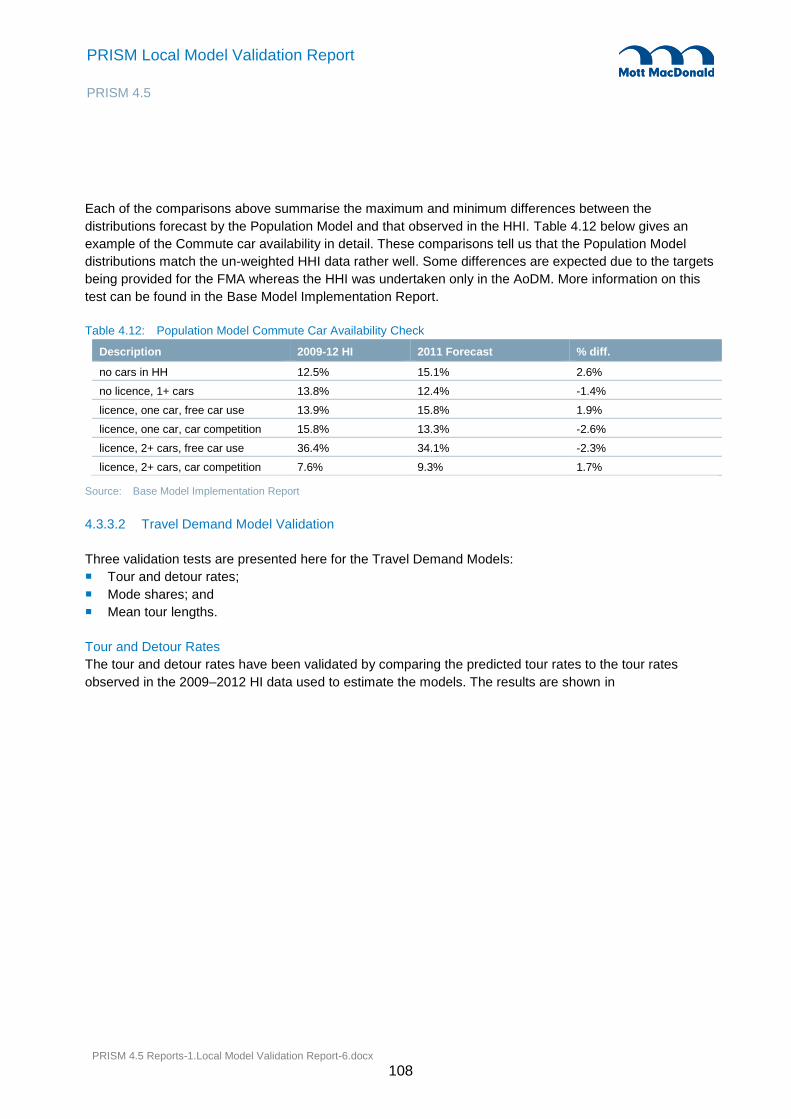
PRISM 4.5 Reports-1.Local Model Validation Report-6.docx
108
PRISM Local Model Validation Report
PRISM 4.5
Each of the comparisons above summarise the maximum and minimum differences between the
distributions forecast by the Population Model and that observed in the HHI. Table 4.12 below gives an
example of the Commute car availability in detail. These comparisons tell us that the Population Model
distributions match the un-weighted HHI data rather well. Some differences are expected due to the targets
being provided for the FMA whereas the HHI was undertaken only in the AoDM. More information on this
test can be found in the Base Model Implementation Report.
Table 4.12: Population Model Commute Car Availability Check
Description 2009-12 HI 2011 Forecast % diff.
no cars in HH 12.5% 15.1% 2.6%
no licence, 1+ cars 13.8% 12.4% -1.4%
licence, one car, free car use 13.9% 15.8% 1.9%
licence, one car, car competition 15.8% 13.3% -2.6%
licence, 2+ cars, free car use 36.4% 34.1% -2.3%
licence, 2+ cars, car competition 7.6% 9.3% 1.7%
Source: Base Model Implementation Report
4.3.3.2 Travel Demand Model Validation
Three validation tests are presented here for the Travel Demand Models:
Tour and detour rates;
Mode shares; and
Mean tour lengths.
Tour and Detour Rates
The tour and detour rates have been validated by comparing the predicted tour rates to the tour rates
observed in the 2009–2012 HI data used to estimate the models. The results are shown in

PRISM 4.5 Reports-1.Local Model Validation Report-6.docx
109
PRISM Local Model Validation Report
PRISM 4.5
Table 4.13 and confirm that, for most of the purposes, the predicted tour rates are very close to those in the
estimation samples. These are generally within 5% for both HB and NHB purposes.
There are a number of significant differences that are accounted for as follows:
As can be seen in

PRISM 4.5 Reports-1.Local Model Validation Report-6.docx
110
PRISM Local Model Validation Report
PRISM 4.5
Table 4.13, for tour and detour rates, there is generally a good match to the HI data for most HB
purposes. However, for home–tertiary education, the application tour rate is significantly lower than the
rate observed in the 2009–2012 HI data. This difference is caused by the lower fraction of full-time
students in the predicted 2011 population compared with the HI data;
For home–escort, the application tour rate is also significantly lower than the rate observed in the HI;
this difference is caused by a higher fraction of individuals in no child households in the predicted 2011
population compared with the HI data; and
Four of the six NHB models validated well, the two significant differences between the predicted and
observed rates are due to the use of mean proportions to implement some of the frequency model
terms.

PRISM 4.5 Reports-1.Local Model Validation Report-6.docx
111
PRISM Local Model Validation Report
PRISM 4.5
Table 4.13: Tour frequency rates validation
Purpose %Diff Purpose %Diff
HB
NHB
commute, S=0 0.20% work–work tours -14.70%
commute, S=3 -1.50% work–other tours -1.60%
commute, S=3,destination sampling -1.50% other–other tours 1.50%
home–business -4.60% work–work detours -2.40%
home–primary -1.90% work–other detours -15.40%
home–secondary -0.20% other–other detours -2.90%
home–tertiary -15.40%
home–shopping, S=0 4.60%
home–shopping, S=3 4.70%
home–shopping, S=3,dest.sampling 4.70%
home–escort -23.90%
home–other travel, S=0 3.30%
home–other travel, S=3 1.70%
home–other travel, S=0 dest.samp. 1.70%
home–other travel, S=0 dest.samp. 1.70%
Source: Base Model Implementation Report
Mode Shares
To calculate a summary measure of the replication of mode share to observed HI data, a root-mean-square
(RMS) measure has been used, defined as follows:
𝑅𝑀𝑆(𝑀) = √∑(𝐻𝐼𝑚 − 𝑇𝐷𝑚)2
𝑀
where:
m represents the modes, with M modes in total;
𝐻𝐼𝑚 are the mode shares from the 2009–2012 HI data;
𝑇𝐷𝑚 are the mode shares predicted by the demand model.
A RMS measure is used by RAND as a standard means of assessing differences between observed and
predicted values. Through the use of a square relationship a higher weight is given to bigger differences,
allowing them to be easily highlighted.
Table 4.14 gives a tabulation of the RMS and confirms that the mode shares are predicted well, with RMS
errors of no more than 4% for most purposes – home-based and non-home-based alike.
Table 4.14: Mode share validation against Root Mean Squares
Purpose RMS(M) Purpose RMS(M)
Home-based
Non-home based

PRISM 4.5 Reports-1.Local Model Validation Report-6.docx
112
PRISM Local Model Validation Report
PRISM 4.5
Purpose RMS(M) Purpose RMS(M)
commute, S=0 1.6%
work–work tours 3.7%
commute, S=3 1.6%
work–other tours 5.3%
commute, S=3,destinationsampling 1.6%
other–other tours 4.1%
home–business 1.3%
work–work detours 3.3%
home–primary 8.2%
work–other detours 0.8%
home–secondary 2.7%
other–other detours 2.4%
home–tertiary 2.7%
home–shopping, S=0 3.3%
home–shopping, S=3 3.2%
home–shopping, S=3,dest.sampling 3.3%
home–escort 2.1%
home–other travel, S=0 3.6%
home–other travel, S=3 3.6%
home–other travel, S=0 dest. 3.6%
Source: Base Model Implementation Report
4.3.3.3 Mean Tour Lengths
A comparison of HI and demand model trip lengths was undertaken for all home-based and non-home-
based purposes which showed that there was a general pattern of over-prediction of tour lengths relative to
the 2009–2012 HI data as shown in Table 4.15 below. However, this can be accounted by the fact that HI
data covered the AoDM only whereas the demand model predictions are for the FMA and longer tour
lengths would be expected in the FMA.
Table 4.15: Comparison of mean tour and detour lengths between HI and demand model
Purpose HI Data (km) Demand Model (km) Difference
Home based
commute, S=3,destination sampling 22.5 24.5 8.9%
home–business 68.3 64.9 -5.0%
home–primary 5.2 5.2 0.9%
home–secondary 8.1 9.6 18.5%
home–tertiary 19.8 24.3 22.9%
home–shopping, S=3,dest.sampling 10.3 10.9 6.1%
home–escort 7.3 6.8 -7.5%
home–other travel, S=3,dest.sampling 18.4 18.1 -1.4%
Non-home based
work–work tours 59.6 61.8 -11.1%
work–other tours 7.4 8.9 -1.9%
other–other tours 8.5 9.6 29.1%
work–work detours 18.9 22.9 -6.9%
work–other detours 9.5 10.2 -2.0%
other–other detours 6.2 5.3 -3.3%

PRISM 4.5 Reports-1.Local Model Validation Report-6.docx
113
PRISM Local Model Validation Report
PRISM 4.5
Source: Mott MacDonald
4.3.3.4 Parameter Values
The disaggregate models in PRISM work with utility functions, rather than generalised cost. These are
similar in concept to generalised cost, but include things like socio-economic terms, destination constants
etc. in addition to (monetary) cost and travel time contributions. A further complication is that the PRISM
models work with non-linear cost formulations (effectively cost damping) which means that the effective
lambda values vary with the cost (distance) of the journey.
In the mode-destination report, the full model results are recorded.18 The most relevant terms are the in-
vehicle time parameters, the cost parameters and definitions of the cost functions, and the structural
parameters that govern the relative sensitivity of mode and destination choice.
Below we have provided the PRISM parameters in equivalent lambda values for sensitivity to car time. The
values were derived by multiplying through by the structural parameters to convert from sensitivities at the
destination choice level to those at the mode choice level. The lambda values are provided in Table 4.16
and Table 4.17 below.
Table 4.16: Destination choice lambdas
WebTAG
Purpose λd min median max
Commute 0.056 0.054 0.065 0.113
Business 0.034 0.038 0.067 0.106
Shopping 0.183 0.074 0.090 0.160
Other travel 0.074 0.074 0.090 0.160
Source: RAND Europe
Table 4.17: Mode choice thetas
WebTAG
Purpose θM_D min median max
Commute 0.78 0.50 0.68 0.83
Business 0.19 0.26 0.45 0.65
Shopping 0.42 0.27 0.53 1.00
Other travel 0.27 0.27 0.53 1.00
Source: RAND Europe
Destination choice and mode choice values are not available for the shopping purpose in WebTAG, so the
values for other travel have been listed for this purpose in the tables above. As shopping is a proportion of
the ‘other travel’ category, a weighted average of the lambda values for shopping and other travel would
give a value which is close to the median destination choice lambda value and within the acceptable range
of mode choice theta values in WebTAG.
18 Mode-Destination Model Estimation

PRISM 4.5 Reports-1.Local Model Validation Report-6.docx
114
PRISM Local Model Validation Report
PRISM 4.5
4.4 Realism Testing
4.4.1 Acceptability Guidelines
WebTAG Unit 3.10.4 (M2) sets out guidelines for checking that a variable demand model behaves
realistically. These checks are made by running tests where various components of travel costs and times
are changed and the overall impact on demand response investigated. The tests are called realism tests
and are undertaken for the base year model. The measure of demand response is called the demand
elasticity which is calculated as follows, where 𝑇 is demand, 𝐶 is cost, and the subscripts 0 and 1 represent
before and after the change in cost respectively.
𝑒 =(log(𝑇1) − log(𝑇0))
(log(𝐶1) − log(𝐶0))
The three so-called primary realism tests described in WebTAG Unit 3.10.4 (M2) and the recommended
demand elasticities for each are as follows:
Car fuel cost: matrix-based and network-based car kilometrage elasticity in the range [-0.25,-0.35] with
employers’ business closer to -0.1 and discretionary trip purposes, e.g. shopping, closer to -0.4;
commuting and education somewhere in the middle. Network-based elasticities lower than matrix-
based;
Public transport fares: public transport demand (trip) elasticity in the range [-0.2,-0.9] with
discretionary trip purposes less elastic than non-discretionary trip purposes, e.g. to place of work; and
Car journey time: car demand (trip) elasticity no stronger than -2.0.
4.4.2 Elasticities
4.4.2.1 Car Fuel Cost
This realism test was implemented by applying a 10% increase to the cost of fuel within the demand model
and HAM. The PRISM VDM was then run for five iterations achieving a demand/supply GAP of 0.138%.
Two elasticity measures were then calculated; one where the kilometrage is calculated based on distance
and demand matrices; and another where the kilometrage is based on summing over links in the HAM.
The car fuel cost elasticities presented in Table 4.18 shows slightly less responsiveness to car fuel costs
than the WebTAG guideline range. The relative elasticities between car work (business) and car non-work
are in line with WebTAG guidelines and the network based calculation is indeed less elastic than the
matrix-based calculation. The model uses local values of time and hence the target fuel cost elasticities for
this model are considered acceptable. This is in line with WebTAG Unit M2 guidelines. The elasticities
shown below are the demand weighted average by time period/user class such that the results represent
the average elasticity for the whole year. Further investigation into the sensibility of these results will take
place later this year, coinciding with a model update to the November release WebTAG value of time.
Table 4.18: PRISM VDM Car Fuel Cost Elasticities
Matrix-Based
Network-Based
Car Work Car Non-Work Car All Car Work Car Non-Work Car All

PRISM 4.5 Reports-1.Local Model Validation Report-6.docx
115
PRISM Local Model Validation Report
PRISM 4.5
Matrix-Based Network-Based
AM -0.12 -0.3 -0.27 -0.07 -0.28 -0.25
IP -0.12 -0.24 -0.2 -0.08 -0.23 -0.19
PM -0.15 -0.29 -0.26 -0.09 -0.26 -0.23
12-hour -0.13 -0.28 -0.24 -0.08 -0.26 -0.22
Source: Mott MacDonald
4.4.2.2 Public Transport Fare
This realism test was implemented by applying 10% increases to the PT fares that are input to the demand
model. The PRISM VDM was then run for seven iterations respectively achieving a demand/supply GAP of
0.04%.
Due to an error in the PT pivoting process that was not fixed until PRISM 4.6, the results can only be
examined from the raw demand model outputs. These are presented below
Table 4.19: PRISM VDM Public Transport Fare Elasticities
Purpose-model Train Metro Bus All PT
HomeBus -0.49 -0.26 -0.22 -0.27
HomeEscort -0.93 -0.93
HomeShop -0.11 -0.04 -0.14 -0.14
HomeWork -0.17 -0.01 -0.34 -0.31
HomeOther -0.16 -0.09 -0.15 -0.15
Airport_BIZ -0.00 -0.09 -0.09 -0.08
Airport_LEI -0.00 -0.04 -0.04 -0.03
HomePrim -0.35 -0.44 0.01 -0.40
HomeSec -0.17 -0.24 0.08 -0.23
HomeTer -0.35 -0.14 -0.14 -0.16
OthOth -0.72 -0.72
OthOthDet -0.44 -0.31 -0.34 -0.34
WrkOth -0.04 -0.04
WrkOthDet -0.51 -0.41 -0.55 -0.54
WrkWrk -0.02 -0.03 -0.02
WrkWrkDet -0.39
-0.33 -0.33
Total -0.19 -0.26 -0.24 -0.24
Source: Mott MacDonald
The total elasticity is within WebTAG guidance, and non-discretionary trips (such as work to work business
trips) have lower elasticities than discretionary trips (such as other to other) which is also in line with
webTAG.
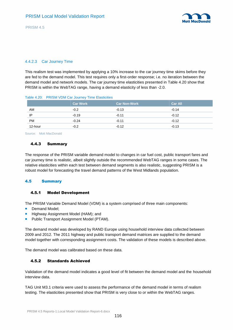
PRISM 4.5 Reports-1.Local Model Validation Report-6.docx
116
PRISM Local Model Validation Report
PRISM 4.5
4.4.2.3 Car Journey Time
This realism test was implemented by applying a 10% increase to the car journey time skims before they
are fed to the demand model. This test requires only a first-order response; i.e. no iteration between the
demand model and network models. The car journey time elasticities presented in Table 4.20 show that
PRISM is within the WebTAG range, having a demand elasticity of less than -2.0.
Table 4.20: PRISM VDM Car Journey Time Elasticities
Car Work Car Non-Work Car All
AM -0.2 -0.13 -0.14
IP -0.19 -0.11 -0.12
PM -0.24 -0.11 -0.12
12-hour -0.2 -0.12 -0.13
Source: Mott MacDonald
4.4.3 Summary
The response of the PRISM variable demand model to changes in car fuel cost, public transport fares and
car journey time is realistic, albeit slightly outside the recommended WebTAG ranges in some cases. The
relative elasticities within each test between demand segments is also realistic, suggesting PRISM is a
robust model for forecasting the travel demand patterns of the West Midlands population.
4.5 Summary
4.5.1 Model Development
The PRISM Variable Demand Model (VDM) is a system comprised of three main components:
Demand Model;
Highway Assignment Model (HAM); and
Public Transport Assignment Model (PTAM).
The demand model was developed by RAND Europe using household interview data collected between
2009 and 2012. The 2011 highway and public transport demand matrices are supplied to the demand
model together with corresponding assignment costs. The validation of these models is described above.
The demand model was calibrated based on these data.
4.5.2 Standards Achieved
Validation of the demand model indicates a good level of fit between the demand model and the household
interview data.
TAG Unit M3.1 criteria were used to assess the performance of the demand model in terms of realism
testing. The elasticities presented show that PRISM is very close to or within the WebTAG ranges.

PRISM 4.5 Reports-1.Local Model Validation Report-6.docx
117
PRISM Local Model Validation Report
PRISM 4.5
5.1 Model Development
The PRISM 2011 highway models have been developed using Visum version 15 as a basis for travel demand
forecasting.
The models have been built with data collected specifically for the purpose of model development, calibration
and validation over the period 2009-2011. Data collected for the development of the base year models
included RSI and public transport surveys to cover trip patterns for all user classes, Trafficmaster data for
high mileage drivers, INRIX data for goods vehicle trip patterns, 2011 household travel survey data for travel
behaviour, automatic and manual traffic counts for link volume flows and bus passengers and journey time
route data.
The highway model includes two car user-classes, LGV and HGV, the public transport model includes two
user classes, fare and no-fare. The models have been built in line with TAG Unit M3.1 guidance for the AM,
IP and PM time periods for an average weekday in 2011.
The highway models incorporate detailed junction coding, blocking back and associated flow metering
effects. The public transport models include all public transport modes. Levels of convergence meet WebTAG
guidelines and the models validate well considering the size of the models.
The variable demand model has been constructed to fit well with the datasets used and is consistent with
NTEM forecasts. The demand model response parameters for frequency, distribution and mode choice
have been calibrated to DfT recommended ranges.
5.2 Standards Achieved
TAG Unit M3.1 criteria were used to assess the performance of the highway models in terms of link volumes,
journey times, screenlines, and changes brought about by matrix estimation and convergence. Whilst the
model does not meet or exceed all validation criteria in all cases, the final models validate well against TAG
criteria, given the size of the model and the quality of the trip matrix has not been compromised to meet the
guideline validation criteria.
For the public transport model, the validation criteria were defined by Centro and Mott MacDonald and are
similar to the WebTAG criteria but account for lower observed counts. The model meets these targets well
and the results are consistent across time periods and different modes of transport.
TAG Unit M3.1 criteria were used to assess the performance of the demand model in terms of realism
testing. The elasticities presented show that PRISM is very close to or within the WebTAG ranges.
5 Summary

PRISM 4.5 Reports-1.Local Model Validation Report-6.docx
118
PRISM Local Model Validation Report
PRISM 4.5
All appendices are contained in PRISM Local Model Validation Report: Appendix, October 2016.
Appendices