Priority Algorithms

Sashka Davis

University of California, San Diegosdavis@cs.ucsd.edu

June 2, 2003

Abstract

This paper reviews the recent development of the formal framework of priority algo-rithms for scheduling problems [BNR02]; the extension of the model for facility locationand set cover [AB02], and graph problems [DI02]. We pose some open questions anddirections for future research.

1 Introduction

Greedy algorithms are a natural approach to optimization. They are simple and efficient.However, a precise formal model of greedy algorithms had not appeared in the literatureprior to the framework of priority algorithms developed in [BNR02]. The definition ofthe formal model of priority algorithms is important because it allows for analysis ofthe power and limitations of a large class of algorithms. The study of lower bounds isimportant because it establishes a negative result about the performance of a large classof algorithms. When the lower bound is tight, the algorithm achieving the desired ratiois optimal for the given class. Lower bounds are useful for the design of an algorithm, asthey guide possible directions for improvements, and serve as an evaluation of the powerof the model. The formal framework of priority algorithms allows us to evaluate a verylarge class of algorithms known in the literature as greedy, and derive non-trivial lowerbounds on the performance of these algorithms for a large domain of problems.

This paper is organized in five sections. First we present the definition of priorityalgorithms as it appeared in [BNR02] and summarize their results. In Section 2 wereview online algorithms and competitive analysis and their relationship to derivinglower bounds on the performance of priority algorithms. In Section 3 we present thefirst extension of the priority algorithm framework for the facility location problem andthe set cover. In Section 4 we present our work generalizing the priority algorithmframework to any problem domain, and applying it to graph optimization problems.And lastly, we pose some open questions and future research directions, in Section 5.

1.1 Greedy and greedy-like algorithms for scheduling prob-

lems

The scheduling problem has been studied for a long time and many of the proposedalgorithms, exact and approximation, are greedy. Are these algorithms the best we can

1

hope for or are there still greedy algorithms that can improve the performance of theexisting ones? To answer this question [BNR02] introduced two formal models of greedyalgorithms, adaptive and fixed priority, which capture the defining characteristics ofgreedy algorithms. Their model only applied to scheduling problems, but was extendingin [AB02] and [DI02] to include almost any combinatorial optimization algorithm. Inscheduling problems, the algorithm is given a list of jobs and must output a solution,which is a schedule of some of the jobs on a set of machines. Later, we will preciselydefine what a scheduling problem is, but for now we would like to focus on the structureof a greedy algorithm for a “general scheduling problem” rather than on the specific pa-rameters and objective functions classifying the different scheduling problems. [BNR02]observed that most (not all) of the greedy algorithms for scheduling problems sharedthe following common features:

• “ one input at a time”. Meaning, that the algorithm considers a single job andhas to make a decision of whether to schedule the job or not. The algorithm doesnot look at the whole instance prior to making a decision.

• the decision of the algorithm is “ irrevocable ”, that is, the algorithm cannotchange its mind later, after observing larger portion of the input.

• the order in which jobs are considered is determined by a priority function, whichorders not just the set of the jobs in the input but all possible jobs.

Based on how often the algorithm gets to re-order the inputs [BNR02] defined fixed andadaptive priority algorithms.

FIXED PRIORITY ALGORITHM

(input: a set of jobs S)Ordering: Determine, without looking at S, a total ordering of all possible jobswhile not empty (S)

next:= index of job in S that comes first in the orderDecision: Decide if and how to schedule job Jnext, and remove Jnext from S

ADAPTIVE PRIORITY ALGORITHM

(input: a set of jobs S)while not empty (S)

Ordering: Determine, without looking at S, a total ordering of all possible jobsnext:= index of job in S that comes first in the orderDecision: Decide if and how to schedule job Jnext, and remove Jnext from S

The previous two models differ in the ability of the algorithm to reorder data inputs.The adaptive priority algorithms have the flexibility to reorder data inputs and can sim-ulate the simple fixed priority algorithms. Based on how the decision is made, [BNR02]defined greedy and not-necessarily greedy algorithms. They called a greedy algorithmone “which makes the decision with the goal of optimizing the objective function as if

the input observed is the last.” That is greedy algorithms locally optimize the objectivefunction. Priority algorithms not-necessarily greedy do not have the restriction on howto make a decision. For example, a greedy scheduling rule will always schedule a job, ifa machine is available. A not-necessarily greedy algorithm may decide to not schedulesuch a job.

A natural question to ask is whether adaptive priority algorithms are more powerfulthan fixed priority algorithms, also is the greedy rule a restriction? [BNR02] proved

2

that the class of adaptive priority algorithms is more powerful than the fixed priorityalgorithms. They did not show a proof of separation between greedy and not-necessarilygreedy algorithms.

Next we will discuss what a scheduling problem is, and some of the results [BNR02]were able to prove. A scheduling problem is defined as a machine configuration, and aninput list of jobs. The algorithm is given a finite set of machines, each machine has adescription of its computation power. The machines could be identical or, some machinescan be parallel. The input to the algorithms is a list of jobs. Each job is described by afour tuple J = (r, d, p, w), where r is the release time, d is the deadline, p is processingtime, and w is the weight or the profit that the algorithm claims if it chooses to schedulethe job. A scheduling algorithm with a given machine configuration must produce anassignment of jobs to machines satisfying a set of constraints. [BNR02] considered non-preemptive scheduling, where once a job is scheduled to a machine it must complete itsexecution. The quality of the solution is determined by the value of the solution for theobjective function specified for the problem. For example, for the profit maximizationproblem the algorithm’s goal is to schedule jobs so that the combined profit of the jobsscheduled is maximized. For the minimum makespan problem the goal is to produce aschedule so that the completion time of the jobs scheduled on any machine is minimized.Although [BNR02] considered a variety of job scheduling problems, maximization andminimization problems, we will present some of their results for the most simple instanceof job scheduling with profit maximization, namely interval scheduling on set of identicalmachines. Interval scheduling is a restricted version of the scheduling problem describedabove, where p = d−r holds for each job in the sequence. The objective function is tomaximize the profit, which is the total length of the intervals scheduled.

Next we summarize some of the interval scheduling results proved in [BNR02]. Proofsof some of the results will be deferred to the next section where we present competitiveanalysis of online algorithms and define a similar framework for proving lower boundsfor priority algorithms.

1. [BNR02] studied the performance of fixed priority algorithms. First they consid-ered interval scheduling for a single machine configuration. They showed that theLongest Processing Time heuristics achieves an approximation ratio of 3. LPTheuristics orders the set of all possible intervals according to their processing timeonce in non-increasing order prior to making any decisions. Then it looks at eachinterval and greedily tries to schedule it, if possible. [BNR02] were able to provethat no priority (fixed or adaptive) can achieve an approximation ratio better than3. This is a good result which shows that a simple greedy heuristic performs opti-mally for both classes of algorithms fixed and adaptive priority, for a single machineconfiguration.

When considering multiple machine machine configurations, [BNR02] showed thatLPT again achieves an approximation ratio of 3 and also they proved that no fixedpriority greedy algorithm can achieve an approximation ratio better than 3. Thisresult shows that the LPT heuristic is optimal in the class of fixed priority greedyalgorithms for a multiple machine configuration.

2. Are adaptive priority algorithms more powerful than the fixed priority algorithms?They are certainly more complex, since the algorithm reorders the remaining inter-vals in the instance prior to making a decision. The answer is yes, adaptation helpsthe algorithm. Recall that no fixed priority algorithm can have an approximation

3

ratio better than 3 for interval scheduling with proportional profit on a multiplemachine configuration (the bound was tight because LPT achieved it). [BNR02]proved that there exists an adaptive priority algorithm, CHAIN-2, which achievesan approximation ratio of 2 on a two machine configuration. They later generalizedthe algorithm for an even number of machines.

The lower bound proved for this class of algorithms, however, is not tight. CHAIN-2 was shown to be a 2-approximation, and the lower bound on the performance

of adaptive priority algorithms is 1 +√

17−32 . Can we close the gap? Is the lower

bound not good enough or there is another algorithm not yet discovered? Theseare questions that remain unanswered.

3. Interval scheduling for arbitrary profits is a difficult problem and both fixed andadaptive perform poorly. The weight (profit) of each interval in the sequence is nolonger proportional to its length. Let ∆ and δ be the maximum and the minimumprofit per unit of all intervals in the instance, respectively, i.e., δi = wi

pi,∆ = maxiδi

miniδi

and δ = miniδi.

[BNR02] showed that no deterministic priority greedy algorithm can achieve aconstant approximation ratio, establishing a lower bound Ω(∆) on the performanceof greedy deterministic priority algorithms. However, if ∆ and δ are known tothe algorithm then randomization helps. [BNR02] presented a randomized fixedpriority not-necessarily greedy achieving an approximation ratio O(log n).

This result is significant because it shows that randomization helps. Thus onedirection for extending the current framework would be to build a formal modelfor randomized priority algorithms.

1.2 Evidence of priority algorithms framework robustness

We would like to know whether the current lower bounds would hold for various exten-sions of the model. A natural extension to the model would be to give the algorithmaccess to global information. This extended model would capture an even larger set ofthe known greedy algorithms, and lower bounds in this model would be very impor-tant. For example, suppose the algorithm knows the length of the instance. [BNR02]proved that their lower bound of 3 on the approximation ratio for the interval schedulingproblem with proportional profit holds for this extended model.

Another interesting extension is to let the algorithm see two inputs (rather thanone) or any fixed number of jobs at a time. They proved a lower bound of 2 on theapproximation ratio of any fixed priority not-necessarily greedy algorithms that can seetwo jobs at a time but must schedule one of them.

2 Online computation, competitive analysis, and

priority algorithms

In this section we introduce online algorithms and competitive analysis. The frameworkfor deriving lower bounds for priority algorithms is borrowed from competitive analysis ofonline algorithms. We will give two examples of deriving lower bounds for deterministicand randomized paging algorithms and then give an example of deriving a lower boundon the approximation ratio achieved by fixed priority algorithms for interval schedulingwith proportional profit.

4

What is an online algorithm? [BEY98] defined an online algorithm as follows: “Inonline computation, an algorithm must produce a sequence of decisions that will have

an impact on the final quality of its overall performance. Each of these decisions must

be made based on past events without secure information about the future. Such an

algorithm is called an online algorithm.” Priority algorithms resemble online algorithms.Both algorithms do not see the whole instance, rather they observe the input one itemat a time. Both algorithms must make an irrevocable decision about a data item, basedon the partial input seen so far. The differences between online algorithms and priorityalgorithms is in the order in which the algorithms see the input. Priority algorithmscan use arbitrarily complex functions to order the data items. In the case of onlinealgorithms, the Adversary or other constraints define the order.

2.1 Competitive ratio

The competitive ratio is a worse-case complexity measurement of the performance ofthe online algorithm as it compares the quality of the solution output by the algorithmto that of the optimal offline algorithm. Suppose we are given a cost minimizationproblem. An online algorithm A is c-competitive if there exists a constant α, whichdoes not depend on the length of the instance, such that for all valid instances I thefollowing holds: A(I) ≤ c · OPT (I) + α, where A(I) is the cost of the online algorithmA on instance I, and OPT (I) is the optimal offline cost on I. The competitive ratio isdefined as the infimum over all constants c such that the algorithm A is c-competitive.

Competitive analysis of online algorithms is viewed as a two player zero-sum game.The players are the Online Algorithm and the Adversary. Zero-sum games best cap-ture the antagonistic relationship between the Online Algorithm and the Adversary.The Online Algorithm seeks to minimize the competitive ratio and the Adversary seeksto maximize it. In what follows we will refer to the Online Algorithm player as theAlgorithm for short.

Consider the following paging problem. We are given a cache with capacity k pages,and a slow memory with capacity N = k + 1 pages. An input to the algorithm is asequence of page requests, say I, where each page is numbered 1, 2, · · · , N . The requestsequence of pages I must be served. If a page requested is in the cache, i.e., the requestis a hit, then the cost of servicing the request is 0. If the request is a miss then a pagefrom the cache must be evicted and the requested page must be swapped in. The costof servicing a miss is 1. The problem is to design a demand paging, page replacementonline algorithm and minimize the total number of pages evicted on any sequence of N

pages.We analyze the performance of the class of deterministic algorithms first, and show

that there is a strategy for the Adversary achieving a payoff of Algorithm(I)Adversary(I) = k Here

we have a cost minimization problem and the Online player seeks to minimize the cost ofthe solution, thus to minimize the competitive ratio. The class of algorithms we considerare deterministic, which means that Algorithm player has chosen a pure strategy fromthe set of all possible strategies prior the beginning of the game. The pure strategychosen is known to the Adversary. The Adversary possesses unrestricted power and canrequest any page so that the cost of processing the request for Algorithm is maximized.One round of the game consists of a request issued by the Adversary and response bythe Algorithm, indicating how the request will be served. That is, Algorithm must showwhich page will be evicted if the request is a miss, otherwise Algorithm does nothing (weare considering performance of demand paging algorithms, only). A winning strategy for

5

the Adversary is to always request the page that Algorithm has evicted at the previousround of the game. The Adversary can choose to end the game at any time. At the end,the Adversary processes the request sequence offline, and the ratio of the online cost tothe offline cost is awarded to Algorithm player.

The strategy described above causes the Algorithm to fault on any page request. Letthe length of the instance I is n then the cost incurred by the Algorithm is A(I) = n.The Adversary serves the entire sequence offline as follows. The cache has size k thusprior to serving the next k requests the Adversary compares his cache with the sequenceand if necessary will swap in the page that that will be requested but is not in his cache.Thus on a sequence of k requests adversary misses at most 1. Thus for a sequence ofn requests the cost for the adversary is at most n

k. The desired ratio Algorithm(I)

Adversary(I) = k

is achieved. Thus we conclude that k is a lower bound on the competitive ratio of anydeterministic online paging algorithm.

2.2 A lower bound for fixed priority greedy algorithms

Proving a lower bound on the performance of priority algorithms is also viewed as arequest-response zero-sum game. Suppose we have a profit maximization problem thenan algorithm A is a c approximation if c ·A(I) ≥ OPT (I) holds for any valid instanceI, where A(I) is the profit gained by the algorithm A, and OPT (I) is the best possibleprofit for the instance I.

To prove a bound on the performance of any fixed priority algorithm, we define arequest-response zero-sum game between two players: the Algorithm and the Adversary.The Adversary is no longer as powerful as before, and the reason is that priority algo-rithms define an order on the data items and this ordering restricts the sets of instancesthat the Adversary can present. In abstract, the game between the Algorithm and theAdversary aims to build a nemesis instance which exhibits the worse performance ofthe Algorithm player. Initially, the Adversary selects a finite set of data items. TheAlgorithm without looking at the set determines an ordering on the data items. Thenthe game proceeds in rounds. At each round the Algorithm looks at the highest prioritydata item and makes a decision. The Adversary may choose to remove data items notyet seen by Algorithm, depending on the the strategy, or may choose to end the game.The payoff to the Algorithm is Algorithm(I)

Adversary(I) , where Algorithm(I) and Adversary(I) arethe qualities of the solutions output by the Algorithm and Adversary, respectively.

We illustrate the technique with an example. We will show a lower bound on theperformance of any priority algorithm for the interval scheduling on a single machinewith proportional profit problem.

1 2 3 q−1q

q−1 3 2 1

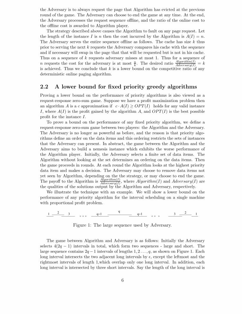
Figure 1: The large sequence used by Adversary.

The game between Algorithm and Adversary is as follows: Initially the Adversaryselects 4(2q − 1) intervals in total, which form two sequences - large and short. Thelarge sequence contains 2q−1 intervals of lengths 1, 2 . . . , q, as shown on Figure 1. Eachlong interval intersects the two adjacent long intervals by ε, except the leftmost and therightmost intervals of length 1,which overlap only one long interval. In addition, eachlong interval is intersected by three short intervals. Say the length of the long interval is

6

p, then the three short intervals for this long interval have length p−2ε3 . Thus the total

number of intervals is 3(2q − 1) + (2q − 1) = 4(2q-1).The Algorithm assigns priorities to the set of all possible intervals. Say i is the

interval with the highest priority. In this particular case the Adversary has a strategyfor the the game and will win after the Algorithm plays his first move:

1. Suppose Algorithm rejects the interval. The Adversary then removes all the re-maining intervals and schedules i. The Algorithm gained profit 0, while the Ad-versary gained profit proportional to the length of i. The payoff to the Algorithmis Algorithm

Adversary= 0

|i| = 0 (The approximation ratio is ∞).

2. Suppose the Algorithm schedules i. The Adversary’s strategy then depends on thelength of the interval i:

(a) If i is a short interval with length p−2ε3 the Adversary removes all but the long

interval intersecting i and schedules the long interval. The Algorithm’s profitis Algorithm = p−2ε

3 . The Adversary’s profit is Adversary = p. The payoff

to the Algorithm is AlgorithmAdversary

= p−2ε3p

(the approximation ratio is 3pp−2ε

).

(b) If i has length 1 the Adversary removes all but the three short intervalscontained by the long interval, and the long interval of length 2 that inter-sects with i. The Algorithm’s profit is Alg = 1. The Adversary’s profit is3 · (1−2ε

3 ) + 2 = 3 − 2ε. The payoff to the algorithm is AlgorithmAdversary

= 13−2ε

(theapproximation ratio is 3− 2ε.)

(c) If i has length j such that 1 < j < q the Algorithm’s profit is Alg = j. TheAdversary removes all but the intersecting intervals and gains profit OPT =j−1+j+1+3 j−2ε

3 = 3j−2ε. The payoff to the Algorithm is AlgorithmAdversary

= j3j−2ε

( the approximation ratio is 3j−2εj

).

(d) At last if the length of i is q Algorithm gains profit q. The Adversary removesall but the intervals intersecting i and gains profit = 2j−2+3 q−2ε

3 = 3q−2−2ε.

The payoff to the Algorithm is AlgorithmAdversary

= q3q−2−2ε

(the approximation ratio

is 3q−2−2εq

).

By making q arbitrarily large and ε arbitrarily small, the Adversary ensures that theapproximation ratio achieved by any priority algorithm is arbitrarily close to 3.

In general, to prove prove lower bounds on performance of priority algorithms wedefine a zero-sum game between the Algorithm and the Adversary. The existence of apriority algorithm with a guaranteed approximation ratio, can be used by the Algorithmas a strategy in the game against the Adversary. On the other hand a strategy forthe Adversary establishes a lower bound. The moves allowed to the Algorithm and theAdversary players are modeled after the structure of the corresponding class of algorithm.For fixed priority algorithms the game has structure such that Algorithm orders the setof data items once. For the remaining rounds, t moves of the Algorithm are decisions fordata items, and moves of the Adversary are modifications of the remaining unseen setof instances. When we want to establish a lower bound on the performance of adaptivepriority algorithms the game is slightly different. During each round the Algorithma data item with the highest priority and makes decision on it. The Adversary thenobserves the move, and based on that information restricts the set of data items accordingto the strategy. The Adversary then decides whether to continue the game or not. Thiscombinatorial game will be illustrated with examples in Section 3 and 4.2.

7

2.3 Lower bound on the performance of randomized pag-

ing algorithms

Next we illustrate the usage of Yao’s technique for proving lower bounds on the perfor-mance of randomized algorithms. For cost minimization problems Yao’s principle statesthat a lower bound on the performance of the best randomized algorithm can be ob-tained by evaluating the performance of the best deterministic algorithm with respectto probability distribution of inputs selected by the Adversary.

We consider the paging problem. Let the size of the cache be k and the number ofpages be N = k + 1. Denote the competitive ratio of any randomized paging algorithmas cR. Our goal is to show that no randomized algorithm can achieve an approximationratio better than Hk, i.e., cR ≥ Hk. To prove a lower bound of Hk on the performanceof the best randomized paging algorithm, it suffices to choose a probability distributionon requests sequences, and to prove that the ratio of the expected online cost of the bestdeterministic algorithm to the expected optimal offline cost is greater than Hk.

1. We must select a probability distribution on inputs. Let P be the probabilitydistribution where: next request ∈u 1, 2, · · · , k + 1. That is any page couldequally likely be chosen as the next request.

2. We evaluate the expected online cost of the best deterministic algorithm. For anydeterministic algorithm and any request of the sequencePr[ request i is a miss ] = 1

k+1 . This holds for the best deterministic algorithm,call it A, as well. Suppose the length of the request sequence I is n. ThenExpP [A(I)] = n

k+1 .

3. We evaluate the expected offline cost. Define a phase as the longest sequence of k

distinct page requests. Then a phase ends before the k +1-st distinct request. Theoptimal offline algorithm can service the k pages in a phase incurring only one mis.Thus we need to estimate the number of phases. Let X(n) be a random variabledenoting the number of phases in a sequence of n requests.ExpP [OPT (I)] = ExpP [OPT (n)] ≤ Exp[X(n) + 1]. For each phase i we let Yi

be a random variable denoting the number of requests in i. Note that Yis areindependent and identically distributed random variables, due to the choice of thedistribution on inputs P.

limn→∞

n

Exp[X(n)]= Exp[Yi]

By the coupon collectors problem Exp[Yi] = (k + 1)Hk

limn→∞

ExpP [A(I)]

ExpP [OPT (I)]=

nk+1n

Exp[Yi]

=Exp[Yi]

k + 1= Hk

We proved that any randomized algorithm cannot achieve an approximation ratio betterthan Hk for the paging problem.

3 Priority algorithms for facility location and set

cover

The first extension of the priority algorithms framework work appeared in [AB02]. An-gelopoulos and Borodin defined a model of priority algorithms for the unrestricted facility

8

location and the set cover problems. Their goal was to define a model of priority algo-rithms for those problems, to prove lower bounds on performance of adaptive and fixedpriority algorithms, and to evaluate the performance of the existing algorithms in theliterature that can be classified as priority algorithms.

[AB02] were able to prove the following tight bounds on performance of adaptive andfixed priority algorithms for unrestricted facility location and set cover.

1. Performance of adaptive priority algorithms for set cover problem.

Slavik showed that the greedy set cover is a lnn−ln lnn + Θ(1) approximation forthe set cover problem. Borodin and Angelopoulos proved that no adaptive priorityalgorithm can achieve an approximation ratio better than lnn−ln lnn+Θ(1). Thegreedy set cover heuristics belongs to the class of adaptive priority algorithms andthus is an optimal algorithm for this class.

2. Performance of priority algorithm for the facility location problem.

• [AB02] considered the uniform metric facility location problem, where theopening costs are identical, and the connection costs obey triangle inequality.They showed that no adaptive priority algorithm can achieve an approximationratio better than 4

3 , when the connection costs are 1, 3. The strategy usedby the Adversary to derive the lower bound above delivers a lower bound ofΩ(log n) for the general facility location problem. This lower bound is matchedby a O(log n) greedy adaptive priority approximation algorithm, showing thatthe bound is tight, and the greedy heuristics is optimal for the class of adaptivepriority algorithms.

• They also were able to show a tight bound of 3 on the approximation ratioachieved by fixed priority algorithms for uniform metric facility location. Thusthe known greedy approximation algorithm is optimal within the class of fixedpriority algorithms.

[AB02] results showed that the best know algorithms for facility location in arbitraryspaces and set cover are optimal within the class of adaptive priority algorithms algo-rithms.

In what follows we will present precise problem definitions and the priority models builtin [AB02] for the problems. Then we prove a lower bound on the approximation ratioof adaptive priority algorithms for the facility location problem.

An instance of the facility location problem is a set of facilities F and a set of citiesC. Each facility has an opening cost fi. For each city j ∈ C a non-negative connectioncost cij represents the charge that must be paid to connect city j to the facility fi. Theproblem is to connect each city in C to a facility in F . The objective function is tominimize the combined connection and opening costs incurred. To build a model forpriority algorithm a specification of the input format and the solution format is needed.[AB02] defined an instance I of the facility location problem to be a set of facilities,where each facility is encoded as a tuple: (fi, ci1, ci2, . . . , ci|C|), where fi and cij are asabove. The solution is a set of facilities S ⊆ F that the algorithm decided to open. Thevalue of the objective function is determined as:

Alg(I) =∑

fi∈S

fi +∑

j∈Cminfi∈S

cij

The first term represents the opening cost incurred by the solution of the algorithm, thesecond term is the combined connection cost.

9

The algorithm chooses the order in which it considers the facilities, and casts irrevo-cable decision, whether to open a facility or not. Once the algorithm chooses to open ornot a facility, it can not change its mind later. The class of adaptive priority algorithmscan re-order the facilities after each decision while fixed priority algorithms determinethe order once.

Next we will show Adversary’s strategy in the zero-sum game, proving that no adap-tive priority algorithm can achieve an approximation ratio better than Ω log n for thefacility location problem in arbitrary spaces. An instance of the problem is a collectionof cities C, and set of facilities F . Let |C| = n, where n = 2k.

We say that a facility fi covers a city j ∈ C if cij < ∞, otherwise we say that thecity j is not covered. Let S be set of facilities that remain in the sequence during anyround of the game between the Adversary and the Algorithm. The Adversary selectsas the initial input set S all possible facilities that cover exactly n

2 cities at cost 1, theremaining cities are not connected, i.e., the cost is∞. The facility opening cost for eachfacility is n. Two facilities are said to be complementary if they together cover all thecities. Obviously, each facility f has exactly one complementary facility f and they areboth in S at the beginning of the game. The game proceeds in rounds. Let C denotethe set of cities not covered by the Algorithm during any stage of the game. Initially,|C| = |C| = n. At the beginning of round t of the game, the Adversary maintainsthe following invariant: 1. The number of the uncovered cities is C = n

2t−1 . 2. Each

remaining facility f ∈ S can cover exactly n2t cities, that is, if f ∈ S at the beginning of

round t then |f ∩ C| = n2t .

Notice that for each f ∈ S then f ∈ S, and thus the remaining facilities can cover theremaining uncovered cities. Obviously, the invariant holds initially. At the beginning ofround 1, the Algorithm has not selected any facilities yet, thus |C| = n, and each of thefacility selected in the initial set by the Adversary covers exactly n

2 cities.At each round:

• Algorithm’s move: The Algorithm selects a facility f from S and decides whetherto open f or not.

• Adversary’s move:

1. If the Algorithm decides to reject the facility then the Adversary removes allthe remaining facility except f and ends the game. The Adversary outputsf, f as a solution, while the Algorithm failed to produce a solution.

2. If the Algorithm decides to open f . Then the Adversary computes C ← C\f .

The Adversary removes from S all facilities covering more than |C|2 cities. That

is f remains in S if |f ∩C| ≤ |C|2 otherwise f is removed. Unless only one city

remained uncovered, in which case the Adversary leaves the set S unchanged.

Claim 1 The invariant is preserved during each round of the game.

Proof: by induction on t. Suppose the invariant holds at the beginning of round t weshow that it is preserved at the beginning of round t+1. If case 1 happens then the gameends. Thus we assume case 2 happens. By the hypothesis, at the beginning of round t

The number of uncovered cities is n2t−1 and all facilities in S are pairs of complementary

facilities such that each facility covers exactly n2t cities. The algorithm chose a facility

in S. Thus the number of uncovered cities at the end of the round is n2t , as wanted.

Then the Adversary removed from S all but those facilities covering exactly half of the

10

n2t uncovered cities. That is each facility f ∈ S covers exactly n

2t+1 uncovered cities.Thus the invariant is maintained at the beginning of round t + 1.

The outcome of the game is either Algorithm fails to produce a valid solution (if case 1was to happen), or Algorithm opened exactly log n facilities at cost n each. In additionthe connection cost for the n cities is 1. Thus the combined cost of the soliton for theAlgorithm is n log n + n. The Adversary opens two complementary facilities and incursopening cost 2, thus the total cost of the Adversary’s solution is 2n+n. And the desiredbound is achieved.

4 Priority models for graph problems

In this section we will review the work on priority algorithms in [DI02]. Our goal was tocapture the defining characteristics of large class of algorithms, known in the literatureas greedy. We defined a general framework of adaptive and fixed priority algorithms, andmemoryless priority algorithms, which is independent of the specific problem domain.The framework can be used to model scheduling problems, facility location problems,graph optimization problems. We abstracted away the information which is specific toencode a job, or a facility, a vertex, or an edge in the graph, and focused on the structureof the algorithms. Then we applied the framework to graph optimization problems andderived lower bounds on the performance of fixed and adaptive priority algorithms. Animportant question to answer is: are the three classes of algorithms needed? Are theyequivalent in power? The existing greedy algorithms for graph problems seem to fit theframework of fixed priority algorithms and memoryless algorithms. Adaptive priorityalgorithms can simulate fixed priority algorithms. We would like to know whether adap-tive priority algorithms are more powerful than fixed priority algorithms. We also wantto evaluate the power of the priority algorithms for specific graph problems. We alsowant to know whether the existing greedy algorithms are optimal or not.

In what follows we show that the three classes of algorithms are distinct.More importantly, we show that imposing a memory restriction on the algorithm

limits its power, that is we prove that memoryless algorithms are less powerful thanadaptive priority algorithms. Precise definition of memoryless algorithms will appear inSection 4.4

4.1 Fixed and adaptive priority algorithms

Assume a generic representation of a graph as a set of vertices, or a set of edges. We viewan instance as a set of data items. Let the type of data item be Γ, thus an instanceas a set of items of type Γ, I ⊆ Γ. Not every subset of data items constitutes a validinstance. Let the set of options (decisions) for each data item be Σ. Then a solutionfor an instance I, can be represented as (γi, σi)|γi ∈ I. For example, for k-colorings ofgraphs on n nodes, we need to assign colors to nodes. So Σ = 1, . . . , k, and Γ shouldcorrespond to the information available about a node when the algorithm has to color it.

A data item corresponding to a vertex can naturally be encoded as name of the node,and the adjacency list of a node, i.e., Γ would be the set of pairs, (NodeName,AdjList),where a NodeName is an integer from 1, . . . , n, AdjList is a list of NodeNames. Moregenerally, a node model is the case when the instance is a (directed or undirected) graphG, possibly with labels or weights on the nodes, and data items correspond to nodes.

11

Here, Γ is the set of pairs or triples consisting of possible node-name, node weight orlabel (if appropriate), and list of neighbors. Σ varies from problem to problem; often, asolution is a subset of the nodes, corresponding to Σ = accept, reject.

For some problems the instance graph is more appropriately encoded as a set of edges.We call this model an edge model. The data items requiring a decision are edges of agraph. In an edge model Γ is the set of (up to) 5-tuples with two node names, node labelsor weights (as appropriate to the problem), and an edge label or weight (as appropriateto the problem). In an edge model, the graph is represented as the set of all its edges.Again, the options Σ are determined by the problem, with Σ = accept, reject when asolution is a subgraph.

As in [BNR02], we distinguish between algorithms that order their data items at thestart, and those that reorder at each iteration. A fixed priority algorithm orders thedata items at the start, and proceeds according to that order. The format for a fixedpriority algorithm is as follows.

FIXED PRIORITY ALGORITHM

Input: instance I ⊆ Γ, I = γ1, ...γd.Output: solution S = (γi, σi)|i = 1, ..d.

- Determine a criterion for ordering the decisions, based on the data items:Choose π : Γ→ R

+ ∪ ∞- Order I according to π(γi), from smallest to largest- repeat

- Let γi be the next data item according to the order- Make an irrevocable decision σi ∈ Σ and update the partial solution S

- Go on to the next data itemuntil (decisions are made for all data items)

- Output S = (γi, σi)|1 ≤ i ≤ d.

Adaptive priority algorithms have the power to reorder the remaining decision pointsduring execution.

ADAPTIVE PRIORITY ALGORITHM

Input: instance I ⊆ Γ, I = γ1, ..γd.Output: solution vector S = (γi, σi)|1 ≤ i ≤ d

Initialize the set of unseen data points U to I, an empty partial solution S, and t to 1.repeat

- Determine an ordering functionπt : Γ→ R

+ ∪ ∞- Order γ ∈ U according to πt(γ)- Observe the first unseen data item γt ∈ U

- Make an irrevocable decision σt and add (γt, σt) to the partial solution S

- Remove the processed data point γt from U and increment t

until (there are no data items not yet considered, U = ∅)

Output S

The current decision made depends in an arbitrary way on the data points seen sofar. The algorithm also has implicit knowledge about the unseen data points: no unseen

12

point has a higher priority under πt than γt.We claim that fixed and adaptive priority algorithms are not equivalent in power and

will prove that next. We define the ShortPath graph optimization problem as follows.Given a directed graph G = (V,G) and two nodes s ∈ V and t ∈ V , find a directedtree of edges, rooted at s. The objective function is to minimize the combined weightof the edges on the path from s to t. We consider the ShortPath problem in the edgemodel. The data items are the edges in the graph. Each edge is represented a triple(u, v, w), meaning the edge goes from u to v and has weight w. The set of options isΣ = accepted, rejected. The well known Dijkstra algorithm which belongs to the classof adaptive priority algorithms solves the single source shortest path (SSSP) problemexactly, thus it can solve the ShortPath problem as well. Next we show that fixedpriority algorithms perform poorly for the ShortPath problem. In the game between theAdversary and the Algorithm player Adversary’s strategy is to force the Algorithm tomake a “wrong” or unfavorable decision. The Adversary can compute the priorities ofthe edges (we are considering fixed priority deterministic algorithms) and is allowed toremove edges from the graph as long as the Algorithm hasn’t considered them. We give

s

z(1)

u(k)y(1)

x(1)

v(1)

w(k)

t

a

b

Figure 2: The initial sequence of data items selected by the Adversary: x, y, z, u, v, w.

short references to data items, for example u is an alias for data item (s, a, k), which isan edge from s to a, with weight k. Depending on the data item selected by Algorithmand decision made, the Adversary restricts S to appropriate subset as follows. TheAdversary can remove data items from the set of instances not yet considered. Since theAlgorithm must assign distinct priorities to all edges. One of the edges y and z mustappear first in the order. We assume, without loss of generality, that the priority of y

is higher than the priority of z, thus the Algorithm would consider y before z. In thiscase the Adversary removes edge v and w from all instances, i.e., S = u, x, y, z. TheAdversary waits until the Algorithm considers edge y. Remember that edge z will beconsidered after edge y. The set of decision options are Σ = accepted, rejected. TheAdversary’s strategy is:

1. The Algorithm decides σy = rejected. Then the Adversary presents the instance:y, v. And outputs solution SAdv(I) = y, v, while the Algorithm failed to con-struct a path.

2. The Algorithm decides sy = taken. Then the Adversary presents y, z, u, x. If theAlgorithm picks edge z, then the Algorithm failed to satisfy the solution constraints.The only valid solution left for the Algorithm is SAlg = y, u, while the Adversary

selects SAdv(I) = z, x. The advantage gained by the Adversary is: ρ = SAdv

SAlg=

k+12 .

13

If the priority of edge z is higher than y then the Adversary removes edges x and u fromthe original graph, leaving edges w, z, v, y and uses the same strategy as before. By givingarbitrarily heavy weights to edges u and w the Adversary can achieve any advantage overany fixed priority algorithm. Thus we proved that no fixed priority algorithm can solvethe ShortPath with any constant approximation ratio. The Dijsktra’s algorithm for thesingle source shortest path problem can be classified as an adaptive priority algorithm.It solves a more general problem, it builds a tree in which the path from a source s

to any other vertex of the graph is minimum, thus it solves the ShortPath problemexactly. Thus we established a separation between the classes of fixed and adaptivepriority algorithms and proved that adaptive priority algorithms are more powerful.

4.2 An example lower bound proof for adaptive priority

algorithms

Next we would like to show an example lower bound proof for adaptive priority algo-rithms to illustrate the adaptive request response zero-sum game between the Adver-sary and the Algorithm. We considered the weighted vertex cover problem. The simplegreedy heuristic achieves an approximation ratio 2 and fits into the adaptive prioritymodel, and we show that no adaptive priority algorithm can do better. Thus the greedy2-approximation algorithm is optimal for the class of adaptive priority algorithms.

We view the set cover in a node model. Here, the algorithm orders nodes basedon their names, weights, and adjacency lists, and must make an irrevocable decisionwhether to include a node in the cover or not. We show a winning strategy for theAdversary player in the zero-sum game between the Algorithm and the Adversary. TheAdversary sets S to be a finite set of Kn,n graphs. Each vertex could have weight w1 = 1or w2 = n2 and is connected to all nodes on the opposite side. An optimum cover is totake the nodes on one side of the bipartite. The Adversary waits until the first time oneof the following three events occur.

• Event 1: The Algorithm takes a node with weight w2 = n2.

• Event 2: The Algorithm rejects a node.

• Event 3: The Algorithm takes n − 1 nodes of weight w1 = 1 from either side ofthe bipartite graph.

If Event 1 occurs the Adversary fixes the weights of all node on the opposite sideto w1 = 1.

If Event 2 occurs the Adversary fixes the weights of all unseen nodes on the oppositeside to w2 = n2 and the weights of remaining nodes on the same side to w1 = 1.

If Event 3 occurs the Algorithm has committed to all but one vertex on one side,say A, of the bipartite graph. Then the Adversary fixes the weight of the last unseenvertex in A to w2 = n2 and remaining nodes on the other side are set to w1 = 1.

Until Events 1 or 2 happen, the Algorithm is taking nodes of weight w1 = 1. Even-tually of the three events, one has to occur. Thus we analyze the performance of thestrategy based on how well the Adversary performs in the different cases.

• If Event 1 occurs first. In this case the Adversary selects all nodes from side B asa Vertex Cover, and the cost of the cover is CAdv = nw1 = n, because until Event1 occurs the nodes are assigned weight w1 and after Event 1 occurs the Adversaryassigns all remaining nodes on side B weight w1. The Algorithm has committed

14

and added a heavyweight node. Therefore Algorithm will incur cost at least n2

which gives a ratio ρ ≥ n ≥ 2.

• If Event 2 occurs first. The Algorithm has rejected node from side A. Algorithmwill have to add all nodes on side B to cover the edges of the rejected node. BecauseEvent 3 hasn’t occurred there must be at least 2 unseen nodes on side B, thereforeAlgorithm will have a vertex cover of cost at least 2n2. Since the Adversary assignsall other nodes on side A weight w1 = 1 the Adversary incurs cost at most n2+n−1by taking all nodes on side A. This give ratio ρ→ 2 as n→∞.

• If Event 3 occurs first. Algorithm has committed to n− 1 nodes on side A. TheAdversary assigns the remaining node on side A weight n2 and all nodes on sideB as w1 = 1. The Adversary takes side B. The optimal choice for Algorithm is totake all nodes on side B as well the n− 1 nodes on side A giving cost 2n− 1. Thisgive ratio ρ→ 2 as n→∞.

We conclude that no adaptive priority algorithm can achieve an approximation ratiobetter than 2 for the weighted vertex cover problem and the greedy 2-approximationalgorithm is optimal within the class.

4.3 Other results

We considered the ShortPath problem for graphs with negative weights, but no negativeweight cycles. This problem can be solved by a dynamic programming algorithm andwe wanted to know whether such a powerful technique was really needed. Could anadaptive priority algorithm solve this problem? We showed that no adaptive priorityalgorithm can solve the problem.

We also considered the independent set for graphs of degree at most 3, and the MetricSteiner tree problems. Here we were not so fortunate and could not prove tight boundsfor these problems on the performance of fixed and adaptive priority algorithms. Weconsidered the Steiner Tree problem for metric spaces in an edge model. The standardfixed priority algorithm for metric Steiner tree (building MST on the subgraph inducedby the required nodes) achieves an approximation ratio of 2. We showed that no adaptivepriority algorithm can achieve an approximation ratio better than 1.18, even for thespecial case where every positive distance is between 1 and 2, and were able to showan improved algorithm for this special case, in the adaptive priority model, achievingapproximation ratio 1.875. The current gap between the lower and the upper bound islarge. How can we close the gap? Can we improve the lower bound? Can adaptationhelp? Are there adaptive priority algorithms that can achieve approximation ratio betterthan 2 for the generic Metric Steiner tree problem? These are questions we hope toanswer.

4.4 Memoryless Adaptive Priority Algorithms

We define a subclass of adaptive priority algorithms, in which the algorithm is restrictedto remember only part of the instance processed. Most of the known greedy heuristicsfor graph optimization problems can be classified as memoryless algorithms so we de-cided to formalize this notion and evaluate the power of memoryless priority algorithmsand compare it to that of adaptive priority algorithms. We want to know whether theexisting algorithms are optimal or not, by comparing the class in which they belongto a different class of algorithms. For this purpose we need to define a formal model

15

of memoryless algorithm and a request-response zero-sum game in which we can provelower bounds. The formal framework of memoryless algorithm is given below.

MEMORYLESS ADAPTIVE PRIORITY ALGORITHMInput: instance I ⊆ Γ, I = γ1, . . . , γd.Output: solution vector S = (γi, σi)| σi = accepted

- Initialization:Let U be the set of unseen data items, S ′ be an empty partial solution,and t is a counter. U ← I; S ′ ← ∅, t← 1.

- Determine an ordering function: π1 : Γ→ R+ ∪ ∞;

- Order γ ∈ U according to π1(γ)repeat

- observe the first unseen data item γt ∈ U .- make an irrevocable decision σt ∈ accepted, rejected .- if (σt = accepted) then

i) update the partial solution: S ′ ← S′ ∪ γtii) determine an ordering function: πt+1 : Γ→ R

+ ∪ ∞iii) order γ ∈ U \γt according to πt+1

- remove the processed data item γt from U : U ← U \γt; increment t← t + 1.until (there are no data items not yet considered, U = ∅)

- Output S ′

What are the differences between memoryless and adaptive priority algorithms?

1. re-ordering the inputs: Priority algorithms with memory can reorder the re-maining data items in the instance after each decision, while memoryless algorithmscan re-order the remaining data items only after casting an accepting decision.

2. state: Memoryless algorithms forget data items that were rejected, while adaptivepriority algorithms have no memory restriction and keep in their state informationabout all data items and corresponding decisions made.

3. decision making process: In making decisions memory algorithms consider allprocessed data items and the decisions made, while memoryless algorithms canonly use the information about data items that were accepted.

The definition of the zero-sum game used to prove lower bounds for adaptivepriority algorithms no longer reflect the capabilities of a memoryless algorithm.Thus a new definition is needed to prove lower bounds. We define a two persongame between Solver and the Adversary to characterize the approximation ratioachievable by a deterministic memoryless adaptive priority algorithm. Let Π bea maximization problem, with priority model defined by µ, Σ, and Γ, where µ isthe objective function, Γ is the type of a data item, and Σ = accepted, rejectedis the set of options available for each data item. Let T be a finite collection ofinstances of Π. The game between the two players Solver and Adversary is asfollows:

Game (Solver, Adversary)

1. Solver initializes an empty memory M : M ← ∅, and defines a total order π1

on Γ.

16

2. Adversary picks any subset Γ1 ⊆ Γ with at least one instance I ⊆ Γ1, I ∈ T ;Sets R← ∅, and a counter t← 1.

3. repeat until (Adversary decides to enter Endgame, or Γt = ∅)begin (Round t)

(a) Let γt be the next data item in Γt according to the order πt

(b) Solver picks a decision σt for γt

• if (σt = accepted) then Solver does the following:

– updates her memory: M ←M ∪ γt

– removes γt from the sequence: Γt ← Γt\γt

– defines a new total order πt+1 on Γ

• else (σt = rejected)

– Adversary updates R← R ∪ γt

– Solver removes γt from Γt: Γt ← Γt\γt

(c) Adversary defines Γt+1 ⊆ Γt.

(d) if Adversary chooses to end the game or (Γt+1 = ∅) then enter Endgameotherwise t← t + 1 and the next round begins.

end; (Round t)

4. Endgame: Adversary presents an instance I ∈ T with M ⊆ I ⊆M ∪ R, anda solution Sadv for I. If no such I exists then Solver is awarded ρ = 1.

5. Solver presents a solution Ssol for I such that M ⊆ Ssol.

6. Solver is awarded the ratio ρ = µ(Ssol)µ(Sadv)

.

We showed that there is a strategy for Solver in the game of incomplete informationdefined above that achieves a payoff ρ if and only if there is a memoryless adaptivepriority algorithm that achieves an approximation ratio ρ on every instance of Πin T . Thus if there is a strategy for Adversary that guarantees a payoff ρ then alower bound is established and there is no memoryless adaptive priority algorithmthat achieves an approximation ratio better than ρ.

We also showed that there is an optimal strategy for Solver that has the fol-lowing property: once Solver rejects one data item, he never accepts any laterdata items by proving that any strategy for Solver achieving payoff ρ, in whichaccepting and rejecting decisions are not separated into distinct phases can beconverted to a strategy achieving the same payoff, in which Solver never acceptsafter it has rejected a data item. Now we can classify most of the known greedyalgorithms in the literature as memoryless adaptive priority algorithms. Viewedin the framework of a game between Solver and Adversary, that corresponds to astrategy of Solver to never accept after a rejection. We would like to know whethermemoryless algorithms are less powerful than adaptive priority algorithms.

We were able to show a separation between the power of the two classes. Welooked at the weighted independent set problem on cycles, and viewed the problemin the node model. A valid instance is a 2−regular graph. Each data item is atriple (name, weight, adjacency list), where |adjacency list| = 2, and weight ∈1, k. We proved that no memoryless adaptive priority algorithm can achieve

17

an approximation ratio better than 2 for the WIS on degree 2 graphs. Since anystrategy for Solver (any memoryless algorithm) can be converted to a strategywith distinct accepting and rejecting phases, then we only need to consider thecases when the first decisions made by the algorithm are accepting.

Adversary selects as a set of instances all pentagons, where the weights of thenodes are 1 or k. Solver must output an order of all possible data items. Thestrategy for Adversary is:

a b

c

d

e

Figure 3: The nemesis graph for MIS problem.

Case 1: Solver picks data item (a, k) first, and decides σ(a,k) = accepted. Then Adver-sary presents the instance: (a, k), (b, k), (c, 1), (d, 1), (e, k). Adversary out-puts the solution SAdv(I) = b, e, while the best Solver can do is SSol(I) =a, c, The advantage gained by Adversary is: ρ = SAdv

SSol≥ 2k

k+1= 2− 2

k+1.

Adversary can choose k arbitrarily large, thus as k → ∞ thus the approxi-mation ratio will be arbitrarily close to 2.

Case 2: Solver picks (a, 1) data item first and decides σ(a,k) = accepted. Then Adver-sary truncates the remaining sequence and presents the instance:(a, 1), (b, k), (c, 1), (d, 1), (e, k). Adversary outputs the solution SAdv(I) =b, e, while the best Solver can do is output SSol(I) = a, c, The advantagegained by Adversary is: ρ = SAdv

SSol≥ 2k

2= 2.

2

To show a separation we exhibited an adaptive priority algorithm for the weightedindependent set problem on 2-regular graphs, achieving an approximation ratio1+ 2

k−1on any instance I, with weights 1, k. This proves that adaptive priority al-

gorithms are more powerful than memoryless algorithms. Can we design improvedapproximation schemes for other graph optimization problems using memory? Theknown algorithms belong to the less powerful class of memoryless algorithms?

4.5 Limitations of the priority algorithms framework

The priority algorithms framework presented above does not capture all the knownalgorithms considered greedy in the literature. Here we give a high level descrip-tion of the best known approximation algorithm for the independent set problemin bounded degree graphs [BF94]. The algorithm proceeds in iterations and at

18

each iteration full knowledge of the input graph is required. The algorithm startsat an arbitrary independent set and looks for an improvement. An improvementis a connected subgraph of size at most O(logn) nodes such that the symmetricdifference of the current independent set with the improvement is a larger indepen-dent set. The algorithm finds improvements by considering all possible connectedsubgraphs. There are at most n∆σ connected subgraphs of size σ of a graph withn nodes and maximum degree ∆. When no further small improvements are pos-sible the algorithm computes a complement of the current independent set andrecursively runs the algorithm on the complemented graph. The bigger of the twoindependent sets are selected. Upon termination, the algorithm guarantees forany ∆ and any k > 0 an approximation ratio OPT (G)

Alg(G)≥ ρ∆ + 1

k, where ρ∆ = ∆+3

5

for even ∆ and ρ∆ = ∆+3.255

for odd ∆. The running time of the algorithm is

n∆O(k.∆4k. log n).Is the algorithm described above a priority algorithm? No, it is not a priority

algorithm. Not according to our current formalization of priority algorithms. Re-call that two of the defining characteristics of priority algorithms are “one inputat a time” and “irrevocable decision”. Both of these conditions are violated bythe algorithm. The algorithm scans the full instance prior to making a decision.Decisions are made for set of data items at a time, since the algorithm is consid-ering improvements. Furthermore, each node is considered many times, and thedecision made is revocable. The algorithm makes a recursive call to itself withthe complement of the current independent set, thus a node which was rejectedinitially could be accepted later, if the independent set built during the recursivecall is bigger than the original IS.

5 Future work

Why is this work important? Because we believe this is a general approach ofevaluating heuristics and algorithm design paradigms by proving lower bounds forall algorithms in a given class. We defined the framework of priority algorithms asa formal model for greedy algorithms. In this framework we were able to analyzethe performance of all the algorithms in the class. Lower bounds establish theweaknesses of the technique while upper bounds determine the kinds of problemsthe technique can successfully be applied.

Can we design formal models for other algorithmic design techniques and frame-works for proving lower bounds? Can we establish both negative results of theirperformance and also identify the strength of the technique and the problems onwhich it performs well? If we build formal models for the known efficient algorithmdesign paradigms (greedy, dynamic programming, hill-climbing) then negative re-sults will show the limits of all natural approaches to optimization.

5.1 Tighten the bounds, and separate the existing models

Many of the current bounds for priority algorithms are not tight. Can the existingupper bounds be improved by designing new algorithms, or are the current lower

19

bounds not good enough? For example, can we obtain an improved lower boundfor the general Metric Steiner tree problem, with unrestricted edge weights? Ourimproved upper bound holds for metric graphs with edge weights 1, 2 only. Whatlower bounds can we obtain for the Maximum Independent Set problems for graphsof arbitrary degrees?

There are problems that we didn’t consider, for example what lower boundscan we prove for the graph coloring problem?

Memoryless priority algorithms were proved less powerful for graph optimiza-tion problems, yet most of the known approximation algorithm are classified asmemoryless algorithms. Can we design improved approximation algorithms usingmemory?

5.2 Extended priority models

Next we would like to extend the priority model and prove lower bounds for thosealgorithms that belong to the extended models. We have seen that there are greedyalgorithms that do not fit the current model of priority algorithms. We would liketo extend the model so that it can capture a larger class of algorithms. For examplewe would like to consider a model where the algorithm is given access to “globalinformation”. The number of nodes or vertices in the graph is global information.What lower bounds can we prove for priority algorithms in this extended model?

Another extension of priority algorithms for graph problems is to redefine the no-tion of local information associated with a data item to span the data items ofit’s neighbors, assuming the problem is viewed in the vertex model. Would thatadditional information, given to the algorithm during the decision-making process,increase the power of the priority algorithms?

Would randomization help? What kind of lower bounds can we prove for random-ized priority algorithms? Our current lower bounds hold only for deterministicalgorithms. How can we apply the developed lower bound techniques for analysisof for online algorithms to proving lower bounds and upper bounds for randomizedpriority algorithms?

5.3 Beyond greedy algorithms

Greedy algorithms are simple and efficient. However, dynamic programming algo-rithms and backtracking algorithms are more powerful. We would like to definesimilar general frameworks that capture the defining characteristics of those pow-erful classes of algorithms.

Let Γ be the type of a data item. A data item can be a vertex, an edge, a job,etc. Let Σ = σ1, . . . , σn be the set of options (decisions) for each data item. Σ isproblem dependent. A backtracking algorithm builds a depth first search pruningtree. We would like to capture this in a formal model. As before we would definetwo classes of algorithms fixed and adaptive, depending on whether the data itemscan be reordered prior to making decisions or not. Thus a fixed backtracking algo-rithm builds the search tree by considering data items in fixed order. The decisions

20

are irrevocable. However, the notion of an irrevocable decision has changed, butnot by much. For each data item a subset of the possible decisions is chosen andthe subset cannot be changed later. Following is an example of what the frame-work of fixed backtracking algorithm might be.

FIXED BACKTRACKING ALGORITHM

Input: instance I ⊆ Γ, I = γ1, . . . , γd.Output: solution vector S = (γi, σi)|1 ≤ i ≤ d

Initialization:Let U be the set of unseen data items U ← I;S ′ be an empty partial solution S ′ ← ∅;I ′ be an empty partial instance I ′ ← ∅; and t← 1.

Determine an ordering function π : Γ→ R+ ∪ ∞

Order γ ∈ U according to π(γ)Repeat

Let γt ∈ U be the next unseen data item according to π.Let Σt ⊆ Σ be the set of options for γt, where Σt is consistent with the

current partial solution.For each σt ∈ Σt in parallel:

BRANCH on (γt, σt), and simulate the algorithm for remaining γ ∈ U

Update the partial solution S ′ ← S ′ ∪ (γt, σt)Remove the processed data item γt: U ← U − γt;

Increment t← t + 1.until (there are no data items not yet considered, U = ∅)

Output the best solution found.

The algorithm builds a tree. A search tree built by a fixed backtracking algorithm,at level i will make a decision about data item γi which is the i-th according tothe priority function. However the decisions options selected Σt could be differentfor each parallel branch.

Adaptive backtracking algorithms can reorder data items prior to making de-cisions. The decision is irrevocable and the subset of options per data item oncechosen can not be changed. The proposed framework is given below.

ADAPTIVE BACKTRACKING ALGORITHM

Initialization:Let U be the set of unseen data items U ← I;S ′ be an empty partial solution S ′ ← ∅;I ′ be an empty partial instance I ′ ← ∅; and t← 1.

RepeatDetermine an ordering function πt : Γ→ R

+ ∪ ∞Order γ ∈ U according to πt(γ)Let γt ∈ U be the next unseen data item according to π.Let Σt ⊆ Σ be the set of options for γt, where Σt is consistent with the

current partial solutions.

21

For each σt ∈ Σt in parallel:BRANCH on (γt, σt), and simulate the algorithm for remaining γ ∈ U

Update the partial solution S ′ ← S ′ ∪ (γt, σt)Remove the processed data item γt: U ← U − γt;

increment t← t + 1.until (there are no data items not yet considered, U = ∅)

Output the best solution found.

As before the algorithm branches on decision for a data item. However, the deci-sions at different branches could be different and also the order of the remainingitems in the separate branches could differ. We would like to answer similar ques-tions as the ones posed before. Are the two classes of algorithms equivalent inpower? We are interested both in negative results and upper bounds.

Clearly, if a backtracking algorithm is allowed to inspect all the leaves of thetree it would be able to produce an optimal solution. However, we would liketo restrict the computation to polynomially many leaves in the search tree, andrelate the quality of the solutions produced by backtracking algorithms and thefraction of the leaves of the search tree inspected. For example, suppose the lengthof the instance is is n. Let |Σ| denote the number of decision options availablefor each data item. The kinds of claims we would like to prove have the followingformulation:

“Any backtracking algorithm that has at most m total branches will

have an approximation ratio bigger than c− (c−1)m|Σ|n , where n is

the number of data items considered.”

If m = |Σ|n then the approximation ratio is 1. But what what happens to theapproximation ratio c, when m is much smaller than Σn?

References

[AB02] Spyros Angelopoulos and Allan Borodin. On the power of priority algo-rithms for facility location and set cover. 5th International Workshop on

Approximation Algorithms for Combinatorial Optimization, September2002.

[BEY98] Allan Borodin and Ran El-Yaniv. Online Computation and Competitive

Analysis. Cambridge University Press, 1998.

[BF94] Piotr Berman and Martin Furer. Approximating maxumum independentset in bounded degree graphs. SODA, January 1994.

[BNR02] Allan Borodin, Morten N. Nielsen, and Charles Rackoff. (Incremental)Priority Algorithms. Thirteen Annual ACM-SIAM Symposium on Dis-

crete Algorithms, January 2002.

[DI02] Sashka Davis and Russell Impagliazzo. Models of greedy algorithms forgraph problems. December 2002.

22