PRINCIPLES OF FINANCIALENGINEERING

Answers to Exercises

S. NeftciCenter for Financial Engineering,Kent State University, Kent, Ohio

andGlobal Finance Program, New School for Social Research,

New York, New Yorkand

ICMA Centre, University of Reading, Reading, UKand

University of Lausanne, Switzerland

B. Ozcan

First DraftNovember 2004

This first draft will be revised and the answers will be extendedas comments are received.

1

Chapter 1

Introduction

Case Study: Japanese Loans and Forwards

1. Follow Figures 1-1 and 1-2 from the text.

2. Japanese banks borrow in yen, and buy spot dollars from their Westerncounterparties. So, the Western banks are left holding the yen for thetime of the loan (three months, in this case).

The main point is here. In an FX transaction, in this case buyingYen, the purchased currency may have to be kept overnight in a Yendenominated account. The FX is by definition not euroYen, so theseaccounts have to be in a bank Japan. some of these will be Japanesebanks.

3. A nostro account is one that a bank holds with a “foreign bank”. (Inthis case London banks hold Nostro accounts with Japanese Banks inTokyo, for example.) Nostro accounts are usually in the currency ofthe foreign country. Suppose an American bank called Bank A buysEuros from an European bank Bank B. These Euros cannot “leave”Europe. They will be sent to a European bank, say Bank of Europe,to be kept in a Deposit account for the use of Bank A. This would be anostro account of Bank A. Bank Awill have similar nostro accountsin Japan, Australia, etc... to trade Dollar against Yen or Australiandollar.

This allows for easy cash management because the currency doesn’tneed to be converted. Incidentally, nostro is derived from the Latinterm “ours”.

The Western banks may not be willing to hold the Yen in their nostroaccounts because this requires them to hold capital against the yen forregulatory purposes.

Japanese banks being more risky, risk managers may also be againstholding “too much” in a Nostro account in Japan. Note that banksoperate in an environment where others have credit lines against eachother. The “Headquarters” may not want a currency desk to have

2

exposure to Japanese Banks beyond a certain limit. This may forceWestern banks to dump the excess Yens at a negative interest rate.

4. By not holding the yen, the Western banks could potentially lose sig-nificant sums if the bank where the Nostro account is held defaults.For this reason they may prefer to dump the yen deposits and earnnegative yield because they can be more than compensated with theirearnings from the spot-forward trade.

3

Chapter 2

A Review of Markets, Players and Conventions

Exercises

Question 1

Going by swap market conventions, the fixed payments for fixed payer swapsare:

• 100 × .0506 × 1 = USD 5.06 million per year• 100 × .0506 × 1 = Euro 5.06 million per year

Fixed payments for the fixed receiver swaps are:

• 100 × .0510 × 0.5 = JPY 2.55 million per 6 months• 100 × .0510 × 0.5 = GBP 2.55 million per 6 months

Question 2

(a) One could take a market arbitrage position as follows: buy Honeywellshares and sell General Electric shares. If the merger takes place, theHoneywell shares will convert to GE shares - that is, these shares willbecome similar and now one can sell the expensive shares and make aprofit.

(b) You do not need to deposit funds to take this position.

(c) You could borrow funds for this position. You would need to if you donot have any GE shares. If you had them then you could engineer thisshort position through short selling them.

(d) This is different from the academic sense of the word arbitrage. Thatinvolves zero risk and infinite gain. Here we do face a risk (see below)and our gains might be very high - but not infinite!

(e) You would be taking the risk that the merger indeed goes throughsuccessfully.

4

Question 3

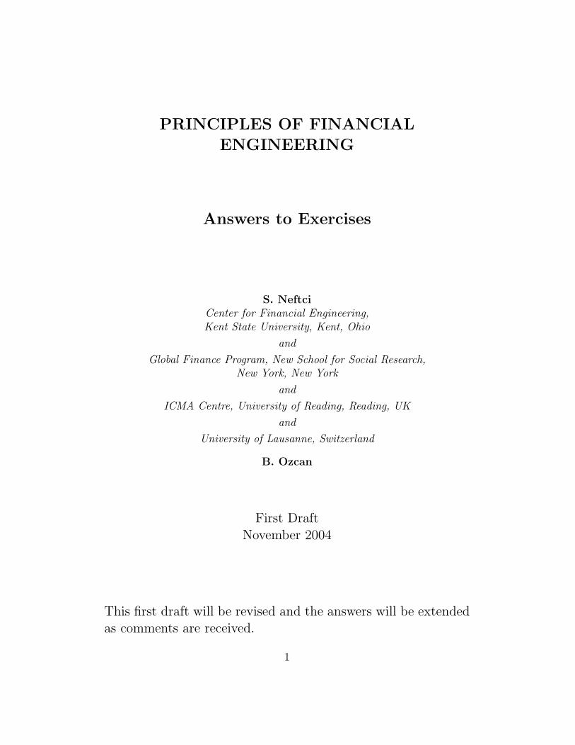
(a) The dealers are selling the Matif contract and buying the Liffe. (Seebelow)

(b) The horizontal axis would have price and the vertical axis would showgain and loss.

(c) Since both Euribor and Euro BBA Libor are both European based rates,the profit would simply be scaled down - if all European interest rateswould be dramatically lowered.

5

Selling Matif

Price

Buying Liffe

Price

Gain

Loss

Gain

Loss

Figure 1:

6

Chapter 3Cash Flow Engineering and Forward Contracts

Exercises

Question 1

(a) Before FAS 133, if companies qualified for hedge accounting, their hedgeswere assumed to be perfect–no valuation or testing required. Now, un-der FAS 133, risk managers seeking hedge accounting treatment have tothoroughly document each hedge from the outset and explain why theyare undertaking the transaction. They have to mark their derivatives tomarket every quarter (no small feat for many instruments), then provethey are effectively hedging the underlying exposure.

It’s this sense of having to pay for the sins of others that accounts for thedeep resentment toward FAS 133. Many finance executives suspect thenew rules have less to do with improving financial statements than withdiscouraging treasury departments from speculating with derivatives.

(b) Constructing synthetic swaps will involve replication of a swap by port-folios of bonds. These do not come under the considerations of FAS 133.So all the work that FAS 133 brings with it needs not be done now.

Question 2

(Parts (a)-(c) answered together:)A gold miner risks losing money if the priceof gold declines, between the time say, when she is mining the gold and whenshe would actually sell it. So, she sells futures. If the market prices fall, shehas still locked in a rate (at the present time, based on the present day valueof gold) high enough for her to make some profit on. This is how she canhedge against a steady decline in gold prices over the years.

Unless she sets a futures price that is lower than the present day value ofgold, she cannot have a loss. And this will typically not happen since thiswould also lead to arbitrage opportunities. But the hedge could lead to a‘loss’ in the sense that if the market price appreciates then she would notmake as much profit as she could have.

7

Question 3

(a) Synthetic for Contract A involves:

‘Sell EUR (to get USD)’ is equivalent to

• Loan: Borrow EUR at t0 for maturity t1

• Spot operation: Buy USD against EUR

• Deposit: Deposit USD at t0 for maturity at t1

Here, t0 is March 1, 2004 and t1 is March 15, 2004. The underlying sumsold is 1,000,000 EUR.

Synthetic for Contract B involves:

‘Buy EUR against USD’ is equivalent to

• Loan: Borrow USD at t0 for maturity t1

• Spot operation: Buy EUR against USD

• Deposit: Deposit EUR at t0 for maturity at t1

Here, t0 is March 1, 2004 and t1 is April 30, 2004. The underlying sumbought is 1,000,000 EUR.

(b) In this part of the question, if we have correctly identified our syntheticswe can simply interpret the data given to us in the question and use thepricing equation (8) from Section 5 of this Chapter. This is given by

Ft0 = et0

B(t0, t1)eur

B(t0, t1)usd

Consider Contract A and its synthetic from the previous part of thisquestion above. We borrow EUR at 2.36%, buy USD at spot rate 1.1500and deposit USD at 2.25%. So,

F 1t = 1.1500 × 2.36

2.25= 1.2062

Now, consider Contract B and its synthetic from the previous part ofthis question above. We borrow USD at 2.27%, buy EUR at spot rate

8

1.1505 and deposit EUR at 2.35%. So,

F 2t = 1.1505 × 2.35

2.27= 1.1910

(c) The basic idea is as follows: now the outright forward spot rate is1.1510/1.1525. With this new rate, consider both synthetics. Long theone that gives you higher profit and short the other. This will givearbitrage.

Question 4

To rank the instruments we need to recall the conventions from Chapter 2.We review Section 5 from Chapter 2, and Table 2-1 in particular. Accordingto the formula given there, we first calculate present day values of theseinstruments.

• 30-day US T-bill: Day count convention: ACT/360. Yield is quotedat discount rate, so we have

B(t, T ) = 100 − RT

(T − t

365

)100 = 100 − 5.5

(30365

)= 99.5479

• 30-day UK T-bill: Day count convention: ACT/365. Yield is quotedat discount rate, so we have

B(t, T ) = 100 − RT

(T − t

365

)100 = 100 − 5.4

(30365

)= 99.5561

• 30-day ECP: Day count convention: ACT/360. Yield is quoted atthe money market yield, so we have

B(t, T ) =100(

1 + RT(

T−t365

)) =100(

1 + 0.052(

30365

)) = 99.5744

• 30-day interbank deposit USD: Day count convention: ACT/360.Yield is quoted at the money market yield, so we have

B(t, T ) =100(

1 + RT(

T−t365

)) =100(

1 + 0.055(

30365

)) = 99.5500

9

• 30-day US CP: Day count convention: ACT/360. Yield is quoted atthe discount rate, so we have

B(t, T ) = 100 − RT

(T − t

365

)100 = 100 − 5.6

(30365

)= 99.5397

Yields on these instruments = 100−B(t, T ), so to arrange these instrumentsin increasing order of their yields, we simply arrange them in decreasing orderof their present day values.

(a) Since we are dealing with an ECP (Euro), the day count convention usedis ACT/360. So there are 62 days till maturity. Also, we have to use themoney market yield rate to compute the present day value. (We haveagain used conventions from Chapter 2, Table 2-1). So,

B(t, T ) = 100 − RT

(T − t

365

)100 = 100 − 3.2

(62365

)= 99.4564384

is the present day of a bond that would yield 100 USD. So, we have tomake a payment of

99.4564384 × 10, 000, 000100

= 9945643.84

US Dollars for this ECP.

10

Chapter 3

Cash Flow Engineering and Forward Contracts

Case Study : HKMA and Hedge Funds, Summer of 1998

The answer below is based on a report submitted by students in theFinancial Engineering Class at ISMA Centre. The text quoted from theseanswers are in italics.

General Background

Hong Kong is a special administrative region of China (HKSAR). It is,arguably, the world’s fourth-largest center for international finance after NewYork, London and Tokyo.

Hong Kong is the world’s ninth-largest international banking center and thesecond largest in Asia, in term of the value of external transactions.

Hong Kong has the world’s tenth-largest securities market and the second-largest in Asia after Tokyo.

Hong Kong’s gross domestic product (GDP) grew by 3% in 1999-comparedwith a decline of 5.1% in 1998(the crisis year)- and grew by a further 14.3%in the first quarter of 2000.

There is no central bank in Hong Kong, instead, the monetary system isone of Currency Board. It is called the Hong Kong Monetary Authority(HKMA). Traders refer to it as “the M-A”. HKMA was created in 1993through a merger of the office of the Exchange Fund and the office of theCommissioner of Banking.

The primary monetary policy of Hong Kong Monetary Authority (HKMA) isto maintain exchange rate stability within the framework of Linked ExchangeRate System through sound management of the exchange fund, monetaryoperations and other means deemed necessary.

11

The Financial Sector In Hong Kong

The financial sector is a key element in the future growth of Hong Kongand a key element in Hong Kong’s financial sector is the exchange regimeadopted by the Hong Kong government. Hong Kong currency is peggedto the US dollar. This is simply referred to as “The peg”.

HKMA doesn’t issue bank notes, bank notes are issued by the three note-issuing commercial banks (NIBs). When the three NIBs issue bank notes,they are required to submit US dollar (at HK$ 7.8 =US$ 1) to the HKMAfor the account of the exchange fund in return for non-interest bearingcertificates for indebtedness (which are required by law as backing for the banknotes issued). The Hong Kong dollar banknotes are therefore fully backed byUS dollar held by the Exchange Fund.

This requirement that notes and coins be fully backed by foreign exchangereserves means that the exchange rate system operates as an example of cur-rency board.

Currency board: is a legal framework that enables local currency to beissued only under strictly limited circumstances. The goal is to ensure thatlocal currency is at all time fully or almost fully backed by reserves of strongcurrency such as the U.S dollar, so that the two become nearly perfect substi-tutes. It involves a legislative commitment to exchange the two currencies ata fixed rate, combined with restrictions on the issuing authority such that newlocal currency is issued only in the presence of sufficient reserves of externalcurrency, so that the exchange commitment is always credible.

In Hong Kong the system differs from pure currency board arrangement, fortwo reasons:

(1) The HKMA has a limited scope for affecting monetary conditions.

(2) Only transaction related with note-issuing purposes between the ExchangeFund and the Note-Issuing Banks (NIBs) are carried out at a linkedexchange rate, whereas all other transactions are conducted freelynegotiated rates.

The principal features of a currency board are as follows:

12

• Discretionary policy in setting the exchange rate is removed.

• Discretionary policy in determining the money supply is limited sinceincreases in the supply of notes in circulation are tied to increases inbank holdings of US dollars.

• Interest rate policy is used for the purpose of augmenting the demandfor local currency. For example, a fall in the demand for Hong Kongdollars can be partly offset by increases in the interest rates in order toencourage the holding of Hong Kong bank deposits rather than repatri-ating the currency for deposits in overseas banks.

Thus, although the currency board system provided stability to the Hong Kongdollar exchange rate, and also to the domestic money supply, it limits the useof monetary policy for other purposes.

In addition, the choice of the “link currency” will also have an impact onthe domestic economy. Movements in the rate of exchange of that currencywith other currencies will affect the exchange rate between the Hong Kongdollar and those other currencies.

What is a Hedge Fund?

A Hedge Fund is a fund established by one or several partners with net worthof at least $1 million (although this maybe falling). It uses long and shortpositions to take speculative positions in multiple markets simultaneously.(Regular equity funds are not allowed by law, to short securities.) Hedgefunds use leverage and trade derivatives in order to maximize returns.

After the leverage effect Hedge Funds command large amounts ofresources. Their positions can significantly affect markets, particularly thosemarkets that are relatively less liquid.

Hedge Fund have been playing a no-lose game

In the simplest strategy a hedge fund borrows Hong Kong dollars(HKD) andthen sells them in the market against USD, i.e., they short the HKD. Notethat this will cause the money supply to shrink. A decrease in money supplyleads to an interest rates increase. Increases in interest rates have severaleffects on the stock market. First borrowing HKD to buy stocks becomes

13

9.5

9.0

8.5

8.0

7.5

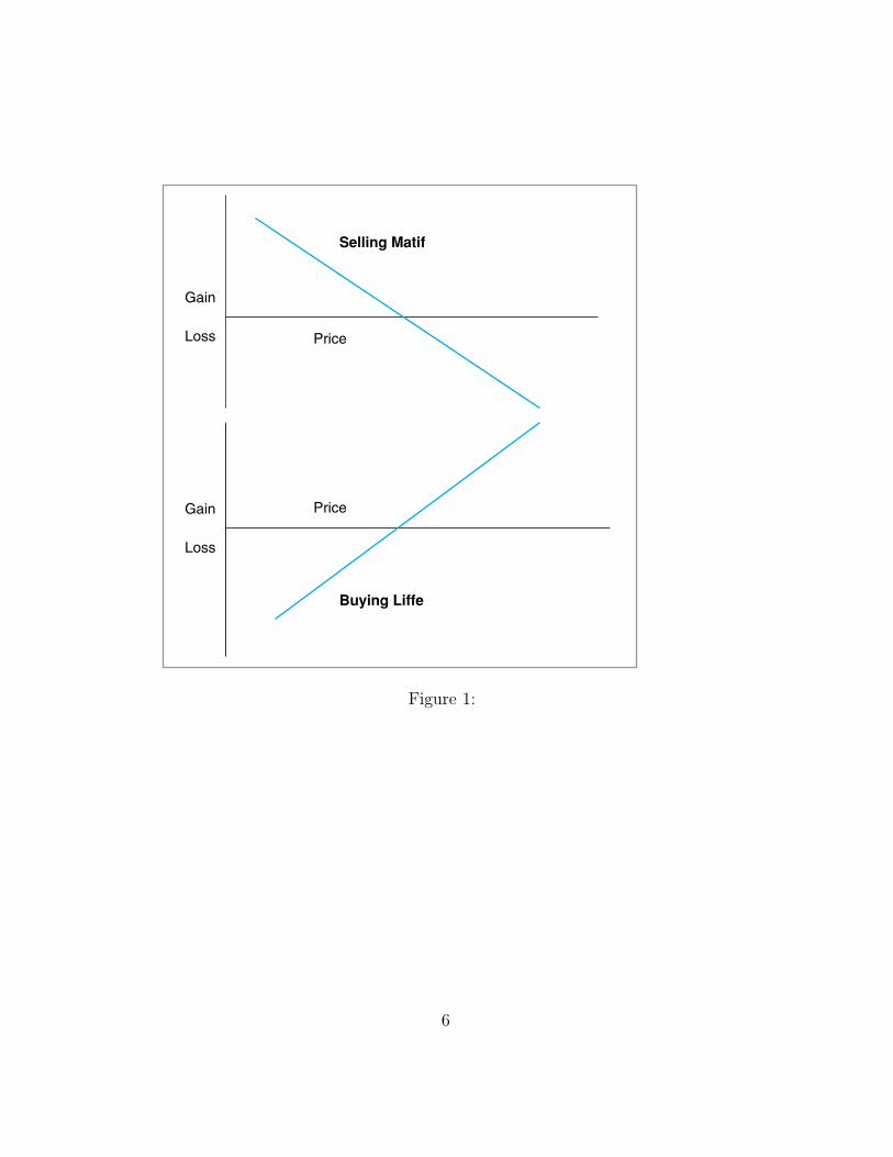
7.0 World stockmarket crash(Oct 1987)

Introduction ofthe linked

exchange ratesystem

(Oct 1983)

Hong Kong dollar/US dollar

Resilience against external shocks

Gulfcrisis(Aug1990)

4thJune1989

Asiancurrencyturmoil

(July 1997–1998)

Mexicancrisis

(Jan 1995)

Closure ofBCCI (HK)(Summer

1991)

ERMturmoil(Sep1992)

6.5

6.0

5.5

5.081 82 83 84 85 86 87 88 89 90 91 92 93 94 95 96 97 98 99

Figure 2:

14

more expensive. Hence fewer investors would use margin. Second, an increasein deposit interest rates will draw funds from stocks to deposits. Third,interest rate increases are negative for businesses and their value will godown. Again stocks decline.

On the other hand, higher interest rates lure more investors to park theirmoney in Hong Kong, boosting the currency. But they also slam the stockmarket because rising rates hurt companies’ ability to borrow and expand.

However, many of these Hedge Funds involved in the speculation did notoperate in the cash market. instead they shorted the HKD in the futuresmarkets. This does not require borrowing HKD. It is the counterparty whohas to hedge the long HKD position who needs to “borrow HKD” from thebanking system.

In the particular case discussed here Hedge Fund managers believed thatthey were taking little risk:

• The hedge funds bet on the collapse of the peg. If the peg breaks, theHKD is expected to fall. Given the psychology of those days, the casualview was that the HKD was overvalued. The only risk to Hedge Fundsis that the peg holds.

Under these conditions their loss will be the difference between theinitial cost of entering the trade to sell HKD in futures markets andthe pegged rate. The reading suggests that this cost is low.

Example: Hedge Fund enters contract to sell HK$ in six month’s. Atexpiration, the Hedge Fund needs to buy spot HKD and deliver these againstthe short future’s position.

If the peg holds the cost of replacing the HKD it has sold is essentiallythe 6 month differential between USD and HKD interest rates.

On Thursday August, 20th the difference in inter-bank interest rates wasabout 6.3%, (Hong Kong rates being higher due to heavy demand for HKDloans, which are needed to short the currency.) So a hedge fund managermaking a USD 1 million bet Thursday against the HKD would have paidUSD63,000.

If the fund manager believed that the peg would break and thus the HKDdepreciate, say, about 30%, then the potential profit would be USD300,000.

15

Compared to the cost of making the trade, USD63,000 this is a good profit.

MA Intervenes HKMA intervened to defend the peg. Using its own FXreserves, MA sold USD. Normally, when a country with a pegged currencyspends reserves to defend the currency’s value, the intervention will have tobe “sterilized”. In other words, the central bank would buy local currencybonds from the banking system. The purchase will be roughly in similarquantities so that the overall monetary base remains constant.

However, doing this in Hong Kong at that time would result in furtherincreases in interest rates. This would be considered as severely harmful byreal estate companies in Hong Kong.

1 PART A

1.1 What is the rationale of the double-play strategy?

The hedge funds deploy a double-play strategy in order to engineer steepincreases in interest rates and steep declines in stock prices so as to gainfrom their short positions in the stock market and in the FX futures market.

But first, some comments abut the economic conditions prevailing at thattime. In early August of 1998, external and domestic conditions deteriorated.The Dow Jones index declined sharply by 300 points on August 5th and theYen was at an eight year low, at 147 on August 11th.

Rumors were abundant concerning abandonment of the peg. There wasstrong selling pressure on HKD early August.

1. Speculators shorted the HKD by swapping HKD for USD.

2. On the equity markets, the stocks index futures market open positionsgrew sharply:

The HSI FUTURES rose from 70,000 contracts in June to 92,000 contractsin August.

The strategy of the Hedge Funds was to undermine the stability of the ex-change value of the HK$ so as to produce sharply higher interestrates.

16

The sharp increases would then lower stock prices, it was hoped. HedgeFunds sell HKD. This increases HKD interest rates(r). Such high interestrates cannot be tolerated by property developers. Real Estate companiessuffer serious losses and their stocks decline sharply. The HSI goes down, asthe HIBOR goes up.

At this point, another strategy is to short sell borrowed shares. Yet, theexistence of futures markets makes this redundant. A speculator can shortthe HSI index instead.

1.2 How are the HIBOR, HSI and HSI futures related?

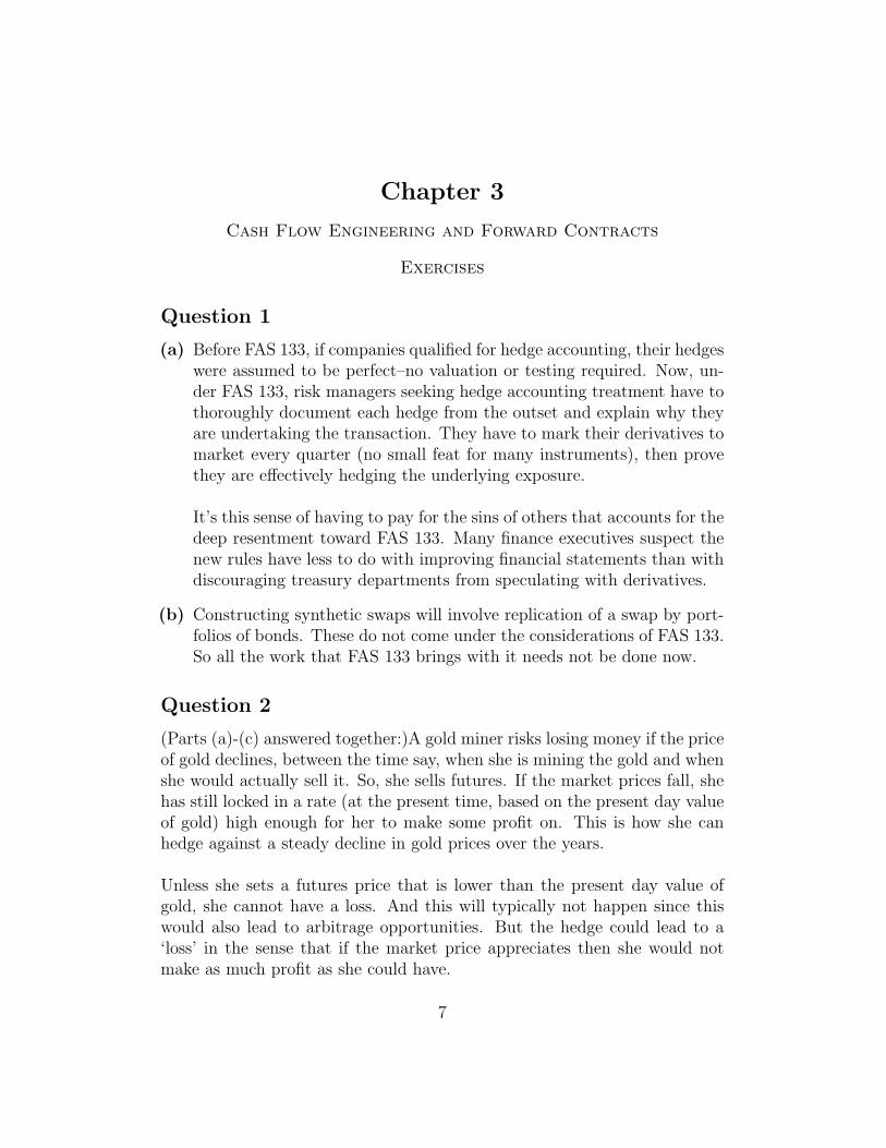
The HIBOR and HSI are inversely related. Consequently futures on HIBORand HSI are also inversely related. See Charts 2 and 3.

HK$/US$

HK$/US$

Effective exchange rate index

Chart 1HK dollar exchange rate (July – September 1998)

Effective exchange rate index

8.20 150

144

138

132

126

120

8.10

8.00

7.90

7.80

7.70Jul Aug Sept

Figure 3: Chart 2

17

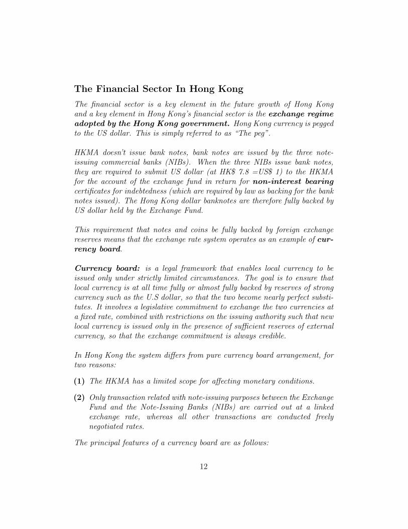
1-month

Chart 3

3-month

14

12

10

8

6

4

2

0

18%

16

Aug SeptJul

Differentials between Hong Kong dollar and US dollar interest rates(July – September 1998)

Figure 4: Chart 3

18

1.3 Display the position explicitly

Example: I borrow 7,800,000 HKD at time t = to at an interest rate rto .

After one year I pay back 7, 800, 000(1 + rto).

At to I exchange these HKD into USD1,000,000. These I deposit at the“risk free” rate Rto .

I expect that The HKD to depreciate 30% during the same time period.

My expected gain is:

Rto1, 000, 000 − rto

78, 000eto(1 + .30)

+ 300, 000

where the eto is the pegged exchange rate, 7.8.

1.4 How is the position rolled over?

As Hong Kong government intervened Hedge Funds decide to just rollingtheir short position over during the month of August. These open positionsare rolled by converting August contracts into September contracts.

The Table below gives further data for this case study.

12 August 19 August 26 August 2 September 9 SeptemberShort term 11.63 12.05 12.33 14.39 8.8

interest ratesUS Federal 5.50 5.59 5.48 5.61 5.47Funds Rate

% Change from −8 11.1 2.8 −6.1 7.5previous week

in the Hang Seng

19

Chapter 4

Engineering Simple Interest Rate Derivatives

Exercises

Question 1

(a) These are just the differences of the two prices. So, the mark to marketlosses are given by {Q1 − Q0, Q2 − Q0, Q3 − Q0, Q4 − Q0, Q5 − Q0}. Ofcourse, negative losses are gains.

(b) You just calculate the interest accrued after multiplying by 1/360 forevery day and,

(c) Then adding the gains and losses.

Question 2

(a) Treasurer has risks for three months starting in three months. So a 3×6FRA is needed.

(b) To get the break even rate we need:(

1 + .0673(

14

)) (1 + f

(14

))=

(1 + .0787

(12

))

(c) Lowest offered rate. (6.87%)

(d) (FRA settlement) (.0687 −.0609)(38 million)(1/4)

Question 3

(a) The futures price has moved by 34 ticks. (It moved from Qt0 = $94.90to Qt1 = $94.56.

(b) The current implied forward rate is given by

Ft0 =100 − 94.90

100= 0.0510

20

which means the buyer of the contract needs to deposit

100(

1 − 0.05104

)= 98.725

dollars per $100 dollars on expiry (which is in three months in this case)

(c) In three months the futures price moves to Qt1 = $94.56 giving a impliedforward rate of

Ft1 =100 − 94.56

100= 0.0544

and a settlement of

100(

1 − 0.05444

)= 98.64

So the buyer of the original contract receives a compensation as if shewere making a deposit of $98.725 and receiving a loan of $98.64, makinga loss of

98.64 − 98.725 = −0.085 per $100 dollars ⇒ Loss of $595000

since the sum involved is $7 million.

Question 4

(a) The trader will buy (sell) the Libor-based FRA, and sell(buy) Tibor-based FRA. This way the market risk inherent in the Libor positionswill be eliminated to a large degree. However, Tibor and Libor fixingsoccur at different times, so there still some risk in this position.

(b) Use two cash flow diagrams, one for Libor FRA the other for the TiborFRA. In one case the trader is paying fixed and receiving floating. Theother cash flow diagram will display the reserve situation. In this setting,the two fixed rates are known and their difference will remain fixed. Thetrader will have exposure to the difference between the floating rates.

(c) If Libor panel is made of better-rated banks, then the Libor fixings willbe lower everything else being the same. This means that the spreadbetween Libor and Tibor will widen. According to this, traders need tobuy the spread if they decide to take such a speculative position.

21

Question 5

(a) To use the given data to create a 1 × 4 NZ $ FRA, the overall strategywould be:

• Replicate the forward borrowing in NZ $ by combining FX for-wards at 1 month and 4 month with spot borrowing of A $ in thefuture (1 month - 4 month) plus a 1 × 4 A $ FRA.

• After we obtain the synthetic forward borrowing in NZ $ via theA $ FRA market, we retrieve the synthetic 1 × 4 NZ $ FRA.

The eventual complete contractual equation could be summarized as:

1 × 4 NZ$ FRA equals:

1. Spot lending NZ $ at t1 = 1 month till t2 = 4 months at rate LNZt1

.

2. Forward sale A $ at t1 = 1 month.

3. Forward purchase of A $ at t2 = 4 month.

4. Spot borrowing of A $ at t1 = 1 month till t2 = 4 month at rateLA

t1

5. 1 × 4 A $ FRA

Note that we can leave out the spot lending and spot borrowing out ofthe contractual equation since they are spot operations.

(b) Left as exercise - use each of the 5 points from part (a) of the questionto describe a cash flow.

(c) This position involves spot lending and borrowing in the future (1 to4 month period) at the Libor rate. These spot operations bring withthem additional credit and liquidity risks.

(d) Since a domestic FRA can be replicated by combining an FX FRAwith forward currency transactions and spot lending and borrowing inthe future, FRA markets and currency forwards should be related bysome arbitrage relationships.

These arbitrage relationships are implicit in the contractual equation.The cost of locking in a future domestic borrowing cost should be equal

22

to the cost of combining the domestic and foreign positions that arerequired to build the synthetic FRA.

Question 6

(a) This can be done by taking a cash loan at time t0, pay the Libor rateLt0 , and buy a FRA strip made of two sequential FRA contracts - a(3 × 6) FRA and a (6 × 9) FRA. The cash flow diagrams are left as anexercise.

(b) Let N be the sum to be borrowed. To find the fixed borrowing cost,simply add the costs incurred by:

• The (3 × 6) FRA, since 3.4 > 3.2, so the floating rate is higher.

• The (6 × 9) FRA, since 3.7 > 3.2, so the floating rate is higher.

• The cost from the three month fixed rate loan.

Additional Information on the Libor-Tibor Case Study

The following lists useful information concerning Libor,Tibor and Euribor.These information are obtained from Student answers to the case study, andfrom various official WEB sites. Two useful links are

(1) http://www.bba.org.uk/bba/jsp/polopoly.jsp?d=141(2) http://www.euribor.org/html/content/panelbanks.html

Libor-based instruments play an important role in financial engineering.Readers are recommended to visit these WEB sites.

1. Japan Premium

The Japan premium reflects the fact that Japanese banking system isfragile due to balance sheets of Japanese banks. The domestic system-atic risks leading to the Japan premium consist mainly in:

(a) solvency risk

(b) Liquidity risk

These are due to reduced profitability of Japanese banks and theirretrenchment, to the closure of large troubled banks, to large undis-closed losses of banks during the 90’s.

23

2. Tibor, Libor

Let us introduce what is the BBA LIBOR-yen and the Euro-yen TI-BOR. The BBA Yen LIBOR is the London Interbank Offer Rate fixedby the British Banking Association that reflects the interest rate atwhich banks in the Interbank London market will borrow yen.

The Yen TIBOR is the Tokyo Interbank Offer Rate determined by theFederation of Bankers Associations of Japan (Zenginkyo) and definingthe interest rate at which banks in Japan borrow yen in the JapaneseInterbank market.

Japanese Yen TIBOR is calculated using an Act/365 day basis and itis primarily used for domestic purposes.

Euro Yen TIBOR is calculated using an Act/360 basis and is composedof twelve terms (from 1-month to 12-month). The fixing panel consistsof 18 banks out of which 16 are Japanese. The Zenginkyo has the rightto designate these reference banks and change the number of them ifnecessary according to their financial activities in the Japan OffshoreMarket (JOM) etc. Rates are quoted by the designated banks as being,in their view, the offered rate at which Euro Yen deposits are beingquoted on 360-day basis between prime banks in the JOM.

Calculation of the rates is based on the elimination of the 2 highest and2 lowest rates from quotations and taking the average of the remain-der. In the case when any bank does not indicate its offer rates, thecalculation will be made in the same manner from the quoting banks.

If, everything else being the same, TIBOR is higher than yen LIBOR,then there exist a risk premium associated with default risk of therespective panel member banks.

3. How are LIBOR, TIBOR and EURIBOR determined?

LIBOR stands for London InterBank Offered rate and is the rate ofinterest at which banks offer funds to other banks, in marketable size,in the London interbank market. It is the primary benchmark used bybanks, securities houses and investors to fix the cost of borrowing in themoney, derivatives and capital markets around the world. LIBOR refersto any of a number of short-term indicative interest rates compiled bythe British Bankers Association (BBA) at 11:00 AM London time, eachbusiness day. LIBOR is quoted for one-week, two-week and monthly

24

maturities up to a year for many of the world’s currencies (Euro, USDollar, GB Pound, Yen, Swiss Franc, Canadian Dollar, and AustralianDollar), as well as spot/next (but overnight for EUR, GBP, USD andCAD).

All currencies are fixed on a spot basis on each London Business Dayapart from GBP, which is fixed for same day value.

LIBOR fixing evolved in the early 1980’s with the growth of syndicatedlending and early developments in the derivative markets. Since, it hasassumed an increasing importance. it is generally acknowledged as atruly international benchmark. BBA LIBOR is published simultane-ously on more than 300,000 screens throughout the world.

The number of contributing banks, quotation basis and fixing basis foreach currency is given in the following table.

Number of Contributors Quotation basis Fixing basisAUD 8 a/360 spotCAD 12 a/360 spotCHF 12 a/360 spotEUR 16 a/360 spotGBP 16 a/365 same dayJPY 16 a/360 spotUSD 16 a/360 spot

The Euro BBA LIBOR Panel banks are chosen on the basis of marketactivity, perceived market reputation and expertise in the particularcurrency and are surveyed for their views of the market rate. Eachbank contributes the rate at which it could borrow funds, by asking forand then accepting inter-bank offers in reasonable market size just priorto 11 AM. All Contributor Panel bank inputs are published on-screento ensure transparency. Contributed rates are then ranked in order andonly the middle two quartiles (50% of contributed rates) are averagedarithmetically.

The resulting Contributor Panel membership is supposed to reflect theinternational composition of the London market and the substantialtrading in European currencies undertaken by banks based outside theeuro-zone.

25

Rates similar to LIBOR are quoted in other world markets. For ex-ample, EURIBOR stands for Euro InterBank Offered Rate. EURI-BOR interest rates are compiled by the European Banking Federation(FBE—Federation Bancaire de l’Union Europeenne) and are releasedat 11:00 AM Brussels time, each business day. Rates are quoted forone-week and monthly maturities up to a year. EURIBOR is widelyused as the underlying interest rate for Euro-denominated derivativecontracts.

Unlike Euro BBA LIBOR, EURIBOR fixing is based on a conceptof country quota. Each in-zone country has at least one bank repre-sented on the Panel and smaller countries will rotate membership of thePanel amongst their leading commercial banks every 6 months. EURI-BOR has a panel of 57 reference banks: 47 from in-zone countries, 4pre-in banks (HSBC and Barclays are the UK representatives) as wellas 6 international banks (Bank of Tokyo-Mitsubishi, Chase, Citibank,JP Morgan Bank of America and UBS). Every panel bank is requiredto directly input their data no later than 10:45 a.m. (CET) on eachday that the Trans-European Automated Real-Time Gross-SettlementExpress Transfer system (TARGET) is open.

The averaging method of EURIBOR is to discard the top and bottom15% of contributed rates and average the remainder.

26

Chapter 5

Introduction to Swap Engineering

Exercises

Question 1

1. The cash flows of this coupon bond can be separated into 8 separatepayments. The first 7 of these will pay $4 at ti, i = 1, .., 7. The lastpayment will be of size $104. This can be used to create the synthetic:

Coupon Bond = [7∑

i=1

4B(to, ti)] + 104B(to, t8)

Where the B(to, ti) are the time to value of the default-free discountbonds maturing at ti. These bonds pay $1 at maturity.

Hence the price of the coupon bond should equal the value on the righthand side plus a profit margin.

2. In this question the Bi are measured at annual frequencies. However,the underlying cash flows are semi-annual. Hence some sort of interpo-lation of Bi is needed. Using a linear interpolation, and then applyingthe above equality twice we can get the bid-ask prices. For example,the Bid price of the coupon bond can be calculated as:

Bid = 4(.95 + .90 + .885 + .87 + .845 + .82 + .81) + 104(.80)

= 107.52

According to this the coupon bond sells at a premium. This is not verysurprising since, the 8% coupon is significantly higher than the annualrate implied by the term structure.

3. Here one can use either the interpolated data or the original term struc-ture, depending on how one interprets the numbers in 1x2 FRA. Taking

27

these as the FRA rate on an 12-month loan that will be made in oneyear we get the equation:

1 + f(to, t2, t4) =B(to, t2)B(to, t4)

Replacing from the term structure we obtain:

f(to, t2, t4)Bid =.90.88

− 1

= 2.27%

Question 2

1. Note that as Italian Government buys back 30-year bonds, the sovereigncurve will shift “down”, relatively more than the swap curve. Or, thesovereign curve will shift up, less than the swap curve, depending onthe direction of the movement. The typical investor is receiving fixed30-year government yield and paying fixed in the swap market. Thereis also the spread received over Euribor. Such an investor will realizecapital gains if yield curve movements occur as expected.

To see this, note that one can approximate the value, Vt, of the positiondescribed in the second paragraph using:

Vto =30∑i=1

(Rto − (Rto + sto) + .00105)B(to, ti) + 100

where we assume, unrealistically, that the ti run over years. The Rt, st

are the sovereign yield, and swap spread respectively. (This is approxi-mate, since we are applying the same discount factors to Euribor-basedpayments and the sovereign interest payments. Normally, these arerelated to different discounts.) The Libor-based payments have thepresent value of 100, which is shown as the last term on the right handside. It is for this reason that no Lti appear on the right hand side.

Now, if the Italian government buys back the 30-year bonds, we expectthe B(t, ti) to increase. Ceteris Paribus, this will leave the st unchangedand the position will gain. If the spread over Euribor falls in additionto this, the gains will be even higher.

28

2. Yes, the trade in the reading will benefit most if 30-year bonds arerepurchased.

3. This is the standard cash flow diagram. The implied graph will besimilar to parts (a) and (b) of Figure 5-7.

4. Ignoring any differences in day counts and other conventions, this makesthe swap rate equal .06 − .00105 if paid against Euribor flat.

5. Investors enter more of such positions and the swap rate will increasedue to supply-demand, this is equivalent to a decrease in the spreadover Euribor.

Question 3

1. You will draw three separate cash flow diagrams, each representing adifferent swap. Assume for simplicity, that the swaps are against 12-month Libor. Remember that the notional amounts are different.

2. For the net payments,one can simply add vertically the cash flows ateach ti.

3. Once these cash flows are determined for each ti, one would multiplythem with the appropriate discount factors, obtained from the swapcurve.

For example, the cash flows two years later, at t2, will be given approx-imately by:

(.0675 − .0675)(50m) + (.07 − .0688)(10m) − (.0755 − .0745)(10m)(1 + .0675)2

The point to remember is that, the unknown Libor-based payments canbe replaced by the corresponding values measured using the currentswap rate given in the Table.

Note that the Swap curve starts at year 2 and some form of interpola-tion is needed for the first year cash flows. Alternatively a Libor curvewill be needed.

4. This will be positive as the above example shows.

29

5. One could hedge the net position that has a five year maturity witha 4-year swap only in an approximate sense. One would calculate thedurations of the two swaps and then take a position that equates thefirst order sensitivities of the net position and the hedge.

6. An exact hedge can be put together by entering into 5 different FRAcontracts.

Question 4

1. The question implies that the ti are measured at annual intervals. Usingthis we can easily calculate arbitrage-free bid-ask prices for the two zerocoupon bonds. For example,

Bask2 =

1(1 + .0810)(1 + .0901)

= .8486

Bbid2 =

1(1 + .0812)(1 + .0903)

= .8483

Note that there is a small arbitrage possibility. One can buy the syn-thetic bond at .8486 and sell the actual bond for .85 at the quotedprice. This will leave a gain of .0014.

2. Three period swap rate will be a weighted average of the quoted forwardrates:

so =2∑

i=0

ωifi

where the ωi are given by:

ωi =Bi+1

B1 + B2 + B3

The key point in applying this formula is the following. Instead of usingthe Bi quoted by the dealer, one needs to calculate arbitrage-free bondprices as in part (a) of this question.

30

Question 5

Additional data on USD and EUR FRA’s will not be directly relevant forfinding arbitrage opportunities in the GBP sector. However, they will berelevant if one had in addition, quotes on forward GBP/USD and forwardGBP/EUR exchange rates. Such forward rates incorporate not one, but twoterm structures and the additional data might help.

Question 6

1. The foreign investor is subject to withholding tax if the issuer is aresident of Australia. In this case the question suggest that the Spanishissuer is not a resident institution. So, the foreign buyer is not subjectto withholding taxes.

2. A resident issuer who would like to issue AUD bonds, can issue in adifferent currency and then swap the proceeds with a foreign issuer. Inthis case the foreign issuer is issuing in AUD and swapping to the othercurrency. Hence there will be two fixed rate swaps and a currency swapthat will have to be involved.

3. With the data provided in this question no precise numerical answercan be given. However, the arbitrage gains will be within 10% of thequoted rates.

4. FRA’s themselves are not sufficient. One would need in addition theproper forward exchange rate contracts on, say, the USD/AUD. Onewould also need the USD FRAs. Then one can synthetically reconstructall the IRSs and the currency swaps desired.

5. Theoretically they will give the same results. However, FRAs will in-volve a much larger number of contracts and may end up being lessconvenient.

6. The Spanish company will issue in Australia and then swap the pro-ceeds into a desired currency. This will be more “profitable”.

Question 7

1. This is similar to Figure 5-6.

31

2. The bottom part of Figure 5-6 shows this.

3. Here we should first note that the currency swap spreads of around75 basis points are unrealistically high for real markets. For thesecurrencies such spreads were normally around 10-20bp during 2004.

Ignoring this aspect we can see that for the immediate period issuingin EUR and then swapping the proceeds into USD will yield an all-incost that is about 10bp higher for the immediate settlement period,since the issuer will be paying 5.8% in USD after the currency swap.

This issuer will pay USD Libor-90 and then receive EUR Libor flat.

32

Chapter 6

Repo Market Strategies in Financial Engineering

Exercises

Question 1

1. 0% haircut implies the collateral is 30 million EUR and the cashreceived is also 30 million.

2. Now the Bund is more valuable than previously thought: by 101 −100.50 = 0.50. So, a portion of the bonds or equivalent amount of cashmust be returned to the dealer by the borrower of the bond.

3. 2.7%.

Question 2

1. 5% haircut implies the “lender” (of the bond) receives 0.95×10, 000, 000= 9, 500, 000 dollars

2. The dealer earns interest at 2.5% on the $9.5 million he lends. But, thedealer can also re-lend 5% of the borrowed securities with 0% haircutand earn extra interest.

Question 3

1. Dirty price is the clean price plus accrued interest = 97 + 3 = 100

2. On the dirty price.

3. Dollars received

= 0.97 × 10.87

× 40m = 44.59m

(taking into account the exchange rate and the haircut)

4. 3%.

33

Chapter 6

Repo Market Strategies in Financial Engineering

Case Study: CTD and Repo Arbitrage

2 Definitions

1. General collateral (GC)

This is the case of a repo transaction between two parties where theborrower is willing to receive as collateral any of the securities satisfyinga general set of criteria.

The GC rate will be higher than the special Repo rate.

2. Special Repo

The borrower asks for a particular security as collateral. Other similarsecurities are not accepted.

3. Cheapest to Deliver (CTD)

Bond futures are structured so as to result in physical settlement. Theshort who decides to deliver, will have to deliver a physical bond. But,usually, bonds of a certain maturity do not have large sizes to ac-commodate quick deliveries. Hence, the futures contracts will trade ahypothetical contract and then a physical bond that resembles to thetheoretical bond is delivered. For this reason Exchanges designate a setof bonds as belonging to a deliverable basket. Although the amount ofeach bond to be delivered is adjusted1 so that they become similar tothe settlement value of the theoretical bond at expiration, one of thesedeliverable bonds will in general be cheapest to deliver. The shorts willobviously deliver this bond called the CTD instead of more expensiveones to satisfy their liability.

In this case study, the CTD is the 6.5% Bobl (see below) with maturityOctober 2005.

1This is done through the so-called adjustment factor.

34

4. Failure to Deliver

This occurs when a repo or futures counterparty that is short the bond,fails to deliver it will result in a failure to deliver. There are dailypenalties for failure to deliver.

3 Consequences

The fees for failing to deliver in repo markets are 1.33 basis points, whereasthe fees for failing in Futures markets is 40bp. Hence, an agent who is shortin the futures market will be penalized much more than an agent who is shortin the repo market. This means that the shorts in the futures markets maybe more willing to deliver the more expensive bonds instead, if they cannotfind the CTD in the open market.

The strategy works better if the profit from more accepting delivery ofmore expensive bonds is greater than the 1.33 basis points DB will be payingas penalty in the repo market.

The position of the DB will be as follows:

1. Let B(to, T ) denote the price of the CTD at time to. DB will placethis amount with the repo dealer at the repo rate rto . The second legof repo is chosen by DB so as to settle at time t1 − Δ. Where Δ is ashort period of one or two days. On this date, the exchange of cashand bond is reversed and DB receives the repo interest.

2. Assume that DB borrows the cash placed with the repo dealer at thegoing Libor rate Lto .

3. Ignore the mark-to-market in the futures position. The futures positiondoes not involve cash at time to. It is assumed to settle at t1. Notethat according to this, the CTD bonds are supposed to be returned tothe repo dealer before futures contract expires. Hence, at that pointthese bonds will be available in the repo market.

4. Yet, if DB fails to deliver, these bonds will not be available to theshorts.

Let’s now see how this can result in a squeeze.

35

3.1 What is a Squeeze?

According to these positions, DB is long the March 2001 contract. This willput upward pressure on the futures price Fto . But DB is also borrowing theunderlying CTD in the repo market.

Although, originally the bonds are supposed to be returned to the repodealer before the t1, DB fails to deliver in the repo market. This removesthese bonds from the repo market for a few days.

Then, the shorts are either forced to close their positions by offsettingthem with new long positions, which means higher futures prices, or, bydelivering the more expensive bonds from the deliverable basket. Eitherway, DB profits.

The following excerpt is from the BIS Quarterly Review, June 2001. Itdeals with the squeeze discussed in this case study. (See, Anatomy of aSqueeze by Serge Jeanneau and Robert Scott in the above-mentioned BISReview.)

The remarkable success of German government bond contractshas created some difficulties in recent years. Most recently, amarket squeeze on the bobl contract was reported during the firstquarter of 2001. The bobl is the five-year German governmentnote, which is used as the underlying asset for related futuresand options traded on Eurex. A small number of European banksapparently cornered the cheapest-to-deliver (CTD) note for thecontract maturing in March 2001, causing major losses to traderswith short positions.

In futures markets, squeezes occur when holders of short posi-tions cannot acquire or borrow the securities required for deliveryunder the terms of a contract. Delivery does not normally posea problem for traders because the majority close their positionswith offsetting transactions prior to contract expiry. However, atrader who remains short at the contracts expiration is obliged todeliver the specified securities, just as one who remains long musttake delivery.

Because of the difficulty in obtaining transparent prices in bondmarkets, most contracts on government bonds require physicaldelivery. This is in contrast to contracts on interbank rates and

36

equity indices, which are settled in cash on the basis of transpar-ent price indices. Physical delivery requires specification of therange of eligible securities and a pricing mechanism to turn thedifferent securities into equivalent assets.

(...)

In the case of the bobl future, the deliverable securities are Germangovernment notes with maturities between 4.5 and 5.5 years. Toadjust for differences in coupons and maturities, the prices ofthese bonds are multiplied by a conversion factor based on a valu-ation of coupons and principal at an annual yield of 6dates. How-ever, because this adjustment is imperfect, one of the securitieswill always turn out to be cheapest to deliver, depending on thelevel of market interest rates and the slope of the yield curve.

(...)

Squeezes are more likely if the supply of the CTD is small, if thechoice of CTD is highly predictable and if its rotation to otherdeliverable securities is prevented by a lack of issues with fairlysimilar price sensitivities.

(...)

Market circumstances in February 2001 appear to have provideda good opportunity for a squeeze. The CTD was the 6.5% notematuring in October 2005. Open interest in the bobl future rose toover 565,000 contracts by 22 February, amounting to a notionalamount of 57 billion. This was over five times the stock of CTDnotes and about one and a half times the total size of the de-liverable basket. By contrast, the December and September 2000contracts had respectively only 384,000 and 281,000 futures out-standing two weeks before expiry.

The graph below illustrates the dynamics of this squeeze. We see thatopen interest of the March 2001 had increased significantly. At the sametime, we see that the spread between the yield of the CTD and the yieldof the next cheapest bond went down from 3 bp to negative 2 bp. Thismeans that the original CTD became more expensive as the expiration ofthe contract approached.

37

25.10.000

150

300

450

Open interest

SpreadCTD-GCbondin bp

2.5

1.0

20.5

22.0

March 2001

06.12.00 22.01.01 05.03.01

The squeeze in the March 2001 contract(BIS Quaterly Review, June 2001)

Figure 5:

38

4 Hedging the short position

Can shorts use other ways to hedge their risks? Consider first a Total ReturnSwap. A Total Return Swap (TRS) is an exchange of interest and capitalgains(losses) generated by a fixed income security against Libor plus a spread.

According to this in a TRS swap the receiver gains exposure to the unde-rlying bond without any capital and without physically owning the asset.

Clearly, the shorts could hedge their short positions in the CTD bondby entering a TRS. The TRS has to be set up with that particular bond asthe underlying. Of course, the spreads to Libor may already incorporate theprice movements due to the squeeze and the hedge may not, at the end, bevery useful. This especially is the case here, since the counterparty to theTRS deal will have to hedge his or her position and this means getting theCTD in the open market. This party will find out that this particular bondis expensive.

On the other hand, the use of FRA’s will not help the shorts. It is unlikelythat the FRA will move significantly due to this squeeze. Squeezes involveCTD’s that are in relative small sizes when originally issued. A shortage ina small issue will not affect the overall level of bond prices.

4.1 Zero repo rates

When a security is heavily demanded by market participants, the repo dealerswill lend it at an “expensive price”. The way this occurs is by adjusting therepo rate.

Hence, the CTD in this question will be in heavy demand. To receive thisbond in the repo market, shorts will have to surrender their cash at a ratelower than the normal repo rate. At the extreme, the repo rate will approachzero.

On the other hand, the repo dealer is securing funds at a cost of 0% whilelending them with a return of rt1 .

5 Other Readings

There are some other readings on this particular event that the readers mayfind useful. One is “The Banker, October 2001, Traders Squeeze Bobl ”.Another is BID quarterly Reviews, for example, June 2002 issue.

39

An academic paper that helps to understand the mechanics of squeezesand the related dynamics is by John Merrick, Narayan Naik and PradeepYadav, et. al. “Strategic Trading Behavior and Price distortion in a Manip-ulated Market: anatomy of a Squeeze.”

40

Chapter 7

Dynamic Replication Methods and Synthetics

Exercises

Question 1

1. The option has a maturity of 200 days. In order to have 5 steps, the Δmust correspond to 40 days. But, we let a year denoted by 1. In thiscase, using a days convention of act/365, the Δ becomes:

Δ =40365

2. In order to answer this question we need further assumptions aboutthe tree structure. The question implies that the probability of thestate denoted as “up” is constant. To obtain this probability we needto discretize the stochastic differential equation.

One way to proceed is the following. We discretize the continuous timedynamics using the Euler scheme and replace the μ with the risk-freerate. We obtain:

ΔSti∼= [.06Δ + σεti ]Sti−1

where ε is a two-state random variable, states being denoted by “up”and “down” respectively. We have the following two-state dynamicsfor St:

Supti = uSti−1

Sdownti

= dSti−1

whereui = 1 + .06Δ + σεup

Let p be the probability of down state. And assume, a usual that

EPti−1

[ε] = 0

41

Then we have the following equations:

εupp + εdown(1 − p) = 0

which is equivalent to:

(uSti−1)p + (dSti−1)(1 − p) = (1 + .06Δ)Sti−1

where the Sti−1 can be eliminated. At this point we have three unknowns,p, εup, εdown. We need more conditions.

We can let the three to recombine, so that an “up” movement followedby a “down” movement results in the same value as a “down” followedby an “up”:

ud = 1

We can now solve for p, εup or p, εdown. Letting εup = 2Δ gives,

p = .663

εdown = −1.970Δ.

Note that the values of the random up and down movements, εj shoulddepend on the Δ. This is needed since, the variance of this term willhave to be proportional to Δ. This is one consequence of Wt being aWiener process, in the continuous form of the dynamics.

Question 2

1. In this case we would follow the same steps as in Exercise 1, afterreplacing the drift of .06Δ by (.06 − .04)Δ.

2. The tree will be the same as in Exercise 1, until the third step. Then,all values are lowered by 5%.

3. The tree will shift down by 5$ after the third step. This will complicatethe tree since, after the third step the remainder of the tree will becomenon-recombining. The reason is that a constant dollar sum is deductedfrom the relevant Sti and this will correspond to a slightly differentpercentage change for the “up” and “down” states.

42

Question 3

We will solve the problem using the GBP/USD exchange rate of $1.85 USDinterest rates of 1.5% and GBP interest rates of 5.5%

1. The new drift, which will be (0.015−0.055)Δ does not affect the choiceof Δ. We still have Δ = 40/365.

2. Using the same method as in the answer for question 1, we find:

p = .64

εup = 1

εdown = −1.7789

which givesu = 1.0154

d = .985

3. Using the initial point of S1 = 1.85 recursively calculate:

Supi = uSi−1

Sdowni = dSi−1

4. In order to calculate the tree for the European Put we start from thelast step, i = 5. Given that the exchange rate tree is recombining wewill have a recombining tree for the Put option. there will be 5 nodesat step i = 5. These values will be

{u2S, uS, S, dS, d2S}

Using the u, d found in the previous question we can calculate the valuesof the exchange rate at step i = 5 and find the values of the put optiondenoted by Pi by letting:

P j5 = max[1.50 − Sj

5, 0]

where j = 1, .., 5 represent the 5 possible states of the last step. Wecan then work backwards, using the relation:

Pi−1 =1

1 + .04Δ[pP up

i + (1 − p)P downi ]

43

5. The American put requires working backwards in the tree as done in theprevious question. However, at each node we need to check one morecondition. The option holder can, at each node exercise the option.Thus the value of the relevant Pi should be compared with 1.50 − Si.If the latter is greater, then the option will be exercised.

This means that the subsequent values on the tree will have to be letequal to zero. Also, this exercise value will be discounted properly inobtaining the value of P1.

Question 4

1. The existence of many Put writers suggest that, these players’ positionswill lose money when the market drops. To hedge this position, theyhave to sell short the underlying stock in the right amount.

This can be shown by using a standard short Put payoff diagram.

2. A covered put position means, the trader has written a put and thenshorted the underlying by selling delta units of the underlying.

Now suppose the market drops further. the trader is hedged againstthis. But, the drop of the market implies a bigger delta in absolutevalue. So, more of the underlying needs to be shorted. Note that thismeans further sales hitting the market. It is this point that is beingrefuted by the traders in the first paragraph of the reading.

3. Short volatility positions are created by selling options, among others.The same trader can be long volatility somewhere else if they eitherown similar options or if they are long convexity.

4. This is quite possible. Note that cash markets are much smaller thanthe markets for derivatives on the same underlying. Thus the derivativemarket may be marginally short, but this may lead to significant shortsales in the corresponding cash market.

5. The last paragraph of the reading suggests that most players try tocover their volatility positions. This may reduce the need for adjustingthe corresponding delta hedge.

44

Question 5

In order to check whether or not the trees in Figure 7-7 are arbitrage free wewould check whether the equality,

Si−1 =1

1 + rjΔ[Sup

i p + Sdowni (1 − p)]

is satisfied at every node.

45

Chapter 8

Mechanics of Options

Exercises

Question 1

1. The payoff diagrams will look as in Figure 1.

2. Gross payoff at expiry will be:

P (T ) = −min[(1.23 − ST ), 0] + min[(1.10 − ST ), 0]

where ST is the EUR/USD exchange rate at expiration.

3. The net payoff will be given by:

P (T ) − P 1.23 + P 1.10

where P 1.23, P 1.10 are the premiums of the corresponding options.

4. If there is a volatility smile, then the implied volatility of the out-of-the-money put will be higher than the implied volatility of the ATMPut. The trader selling the out-of-the-money volatility and buying theATM volatility. Hence if the “smile” flattens, the trade gains.

Question 2

1. Long gamma means, buying related Puts and/or Calls and then deltahedging these positions with the reverse position in the underlying.The hedge ratio will be gamma. This isolates the convexity of optionpayoffs and benefits from increased volatility.

If markets have not priced-in the increase in volatility that may resultfrom (anticipations of ) FED announcements, then the trade will ben-efit. Realized volatility will be higher than the volatility priced in theoptions. Gamma gains would exceed any interest expense and timedecay during the 7 day period.

46

2. Here we can calculate the gamma of at-the-money options. We canassume interest rate differentials around 3%. We can let the life of theoption be 7 days.

Such ATM options would have maximum gamma, since the price curvewill be very close to the piecewise linear option payoff diagram. Thismeans that the traders are maximizing their exposure to increasedvolatility trough Gamma.

3. Given the volatility, we can approximately calculate possible gains byletting

N∂2C

∂e2t

et7

365(σ2

realized − σ2)

where et is the expected USD/NZD exchange rate and N is the notionalamount which is said to be around USD10-20 millions.

Calculating the Black-Scholes Gamma and then plugging in the rel-evant quantities in the above formula will give approximate size ofexpected gains for various realized volatilities.

Question 3

1. Buying sort-dated euro Puts and the implied Gamma means that traderswill go long EUR/USD exchange rates. Thus they will buy Euro andsell Dollars.

2. Buying euro puts is a hedge for further drops in euro.

3. Triggering of barrier options may lead to relatively large movements.This may or may not increase the realized volatility. If it does, thenbuying Gamma will be the natural response.

Question 4

1. Two very crude approximations for Delta are,

C(S + ΔS) − C(S)ΔS

47

−C(S − ΔS) + C(S)ΔS

A better approximation is

C(S + ΔS) − C(S − ΔS)2ΔS

In fact, applying these to the data shown in the Table we see that onlyin the last case we obtain an ATM delta of around .5. The two othercases give very different ATM Deltas.

2. ATM delta is around .5 as the third method illustrates. We can simi-larly calculate the Delta for spot equal to 25. However, we cannot usethe third method when S = 10, or when S = 30. For these the firstand the second formula need to be used.

Once these deltas are calculated, then we can calculate daily gains/lossesas:

−r1.31

365+

12[Deltat − Deltat−1][St − St−1] + Time − decay

3. In this case the volatility is much higher and the Gamma gains will behigher as well.

Question 5

1. Volga is a Greek relevant for Vega hedging. It is the second derivativeof the option price relative to the volatility parameter,

V olga =∂2C

∂σ2

2. Vanna represent the derivative of the Vega with respect to the spotprice,

V anna =∂2C

∂σ∂St

3. These Greeks can be considered as changes in Vega when volatilityand the underlying spot price change. Hence they will be relevant forhedging and measuring Vega exposures.

48

Payoff

At-the-money put

EUR/US0 1.17

1.10

Figure 6:

49

Chapter 9

Engineering Convexity Positions

Exercises

Question 1

1. By definition, the price of a coupon bond will be given by,

P (0, tn) =

[n∑

i=1

c∏ij=1(1 + y)j

]+

100∏nj=1(1 + y)j

Since the yield curve is flat, yk = y1 for all k. The forward rate, fi, isdefined as

fi =

∏ij=1(1 + y)j

∏i−1j=1(1 + y)j

− 1 = y.

0.03 0.04 0.05 0.06 0.07 0.08 0.09 0.10.01 0.02

250

200

150

100

50

0

Bon

d pr

ice

Bond price

Yield

50

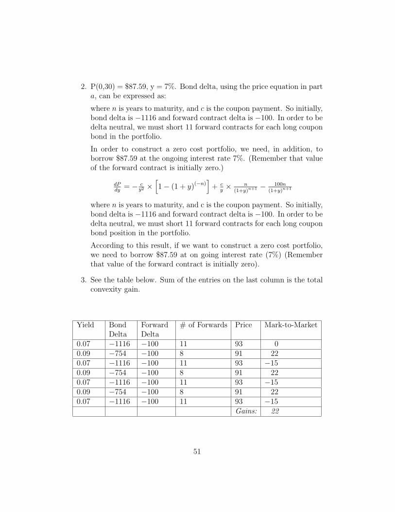
2. P(0,30) = $87.59, y = 7%. Bond delta, using the price equation in parta, can be expressed as:

where n is years to maturity, and c is the coupon payment. So initially,bond delta is −1116 and forward contract delta is −100. In order to bedelta neutral, we must short 11 forward contracts for each long couponbond in the portfolio.

In order to construct a zero cost portfolio, we need, in addition, toborrow $87.59 at the ongoing interest rate 7%. (Remember that valueof the forward contract is initially zero.)

dPdy

= − cy2 ×

[1 − (1 + y)(−n)

]+ c

y× n

(1+y)n+1 − 100n(1+y)n+1

where n is years to maturity, and c is the coupon payment. So initially,bond delta is −1116 and forward contract delta is −100. In order to bedelta neutral, we must short 11 forward contracts for each long couponbond position in the portfolio.

According to this result, if we want to construct a zero cost portfolio,we need to borrow $87.59 at on going interest rate (7%) (Rememberthat value of the forward contract is initially zero).

3. See the table below. Sum of the entries on the last column is the totalconvexity gain.

Yield BondDelta

ForwardDelta

# of Forwards Price Mark-to-Market

0.07 −1116 −100 11 93 00.09 −754 −100 8 91 220.07 −1116 −100 11 93 −150.09 −754 −100 8 91 220.07 −1116 −100 11 93 −150.09 −754 −100 8 91 220.07 −1116 −100 11 93 −15

Gains: 22

51

4. Other costs are funding cost and other operational costs, fees and com-mission paid.

Question 2

1. Price of 30 year bond is,

B(0, 30) =100

(1 + y)30

and it is equal to $23.14 when y = 5%. In order to meet the zero-costcondition, we borrow $23.14 at a rate of 5%. Bond’s delta is given by,

dB

dy= − 3000

(1 + y)31

So initial bond delta is −661 and euro dollar contract delta is −25. Thatmeans for each long bond position, we must short 661

25 euro contracts toachieve delta neutrality, initially.

2. The solution to this problem is very similar to solution given for ques-tion 1, part (d) above. The sum of the entries on the last column isthe convexity gains.

Yield BondDelta

EDDelta

# ofContracts

Price ofED

Mark-to-market

0.05 −661 −25 26 98.75 00.06 −493 −25 19 98.5 6.50.04 −889 −25 35 99 −9.50.06 −493 −25 19 98.5 17.50.04 −889 −25 35 99 −9.50.06 −493 −25 19 98.5 17.50.04 −889 −25 35 99 −9.5

Convexitygains:

13.00

52

Question 3

Interest rate fluctuations are wider in this question compared to previousquestion. That means higher volatility which implies higher convexity gains.So, the total rate of return on this bond will be higher, while interest ratefor 30 year bond decreases.

Question 4

Let f be forward rate on Libor-on-arrears FRA. And F be the forward rateon market traded FRA. Then, existence of convexity requires the followingadjustment between these two forward rates:

f = F + σ2

So the spread is equal to σ2, (0.02)2.

53

Yield YieldY

Bon

d pr

ice

Duration underestin ates

Duration overestin atesfall in bond prices

YTM

Figure 7:

Chapter 9

Engineering Convexity Positions

Case Study: Convexity of Long bonds, Swaps and Arbitrage

1. We now, explain the notion of convexity of long bonds.

For a given decrease in the yield, bond prices will increase more com-pared to the linear approximation of the price-yield relationship. For agiven increase in the yield, bond prices will decrease less compared tothe linear approximation of the price-yield relationship.

The Figure 1 above shows this.

We can also give an example.

Let us find the bond sensitivities for a 3-year bond and a 30-year bondgiven the following conditions:

(a) yo = 6.5% and Δyo = 0.3

(b) y1 = 6.9% and Δy1 = 0.6

where, yo, y1 are the yields of 3 year and 30 year default-free discountbonds, whose prices are denoted by B3 and B30. These prices will be

54

given by:

B3 =100

(1 + yo)3

B30 =100

(1 + y1)30

The first order sensitivities are related to these bonds duration. Forthe short bond this will be given by:

∂B3

∂yo

1B3

= (−3)100

(1 + yo)3+1

=−300

(1 + yo)4

= 3(

1(1 + yo)

100(1 + yo)3

)

= 31

(1 + yo)B3

This means that the percentage in the bond price will be:

∂B3

∂yo

= (−3)100

(1 + yo)3+1

=−300

(1 + yo)4

= 3(

1(1 + yo)

100(1 + yo)3

)

= 31

(1 + yo)B3

∂B3

∂yo

1B3

= 31

(1 + yo)

Hence the term modified duration. The right hand side in this expres-sion gives the slightly modified maturity of the cash payments associ-ated with this security.

55

For the long bond we get:

∂B30

∂y1

1B30

= 301

(1 + y1)

We can use this in order to get approximate measures of bond pricesensitivities. For example:

ΔB3

B3

∼= 31

(1 + yo)Δyo

ΔB30

B30

∼= 301

(1 + y1)Δy1

These measures indicate that, the 30-year bond will be a bout 10 timesmore sensitive to an interest rate change than a 3-year bond, for thesame amount of yield movement.

We can also calculate second order sensitivities. These convexity or“Gamma” effects will show how the first order sensitivities change asthe yield moves.

∂2B3

∂y2o

1B3

= (12)1

(1 + y)2

and

∂2B30

∂y21

1B30

= (930)1

(1 + y)2

Thus, the long bond duration will be about 80 times more sensitive tochanges in the yield when compared with the short bond.

2. Suppose we short the 3-year bond and go long on the 30-year bond.Then, consider three cases where interest rates move up +0.3, staysame or move down −0.3. How will all these affect the bond portfolio?

56

• If interest rates rise we will gain more on the short position of lessconvex bonds than the amount we would lose on the long positionof more convex bonds;

• If interest rates fall we will gain more on the long position of moreconvex bonds than the amount we would lose on the short positionof less convex bonds;

• If interest rates remain unchanged, portfolio’s value will remainthe same.

According to this we are short the lesser convex bond and long themore convex bond. As yields fall the price of this latter rises higherthan the less convex bond and as yields rise its price falls less.

3. Swap convexity will be similar to coupon-bond convexity analysis. Con-sider the following terminology:

(a) st = Swap rate at time t on a swap that starts at t.

(b) n = Number of swap settlements.

(c) δ = Tenor of the floating leg. δ = 1/4 corresponding to a 3-monthfloating rate leg.

(d) N = Notional amount.

(e) Lti = Libor rate to settle in-arrears at time ti+1.

(f) Fti = The FRA rate that corresponds to the floating Libor rateLti .

(g) fixed and floating day basis, both 30/360.

Under these conditions the value of the swap at time, to, will be givenby:

Vto =n∑

i=1

[(Fti−1 − sto)Nδ∏i

j=1(1 + Fti−1)δ

]

Note that this is a convex(concave) function.

57

Note that this gives the discounts Bi as of to as:

Bi =

[1∏i

j=1(1 + Fti−1δ)

]

Now suppose the we consider two swaps with n = 3 and n = 5 respec-tively, with δ = 1. The Swap notional is 10m. The yield curve is flatat 4%. This makes all forward rates equal 4%. Then we can calculatethe following numbers using the formula above.

Changes in thevalue of the swap

Scenario 1 Scenario 2

Type of Swap Parallel Shiftdown 1%

Parallel shift up 1%

3 yr swap - $193,887.49 $ 188,338.21 (value 0 at t = 0)5 yr swap - $376,497.28 $ 358,940.77 (value 0 at t = 0)

From these numbers we see that the 5-year swap is more sensitive tothe changes in the interest rates than 3-year swap; therefore, the tradermight gain more by trading long-dated swaps.

4. We let a Libor-in-arrears instrument pay according to the followingfunction:

Vt = 100(1 − Ltiδ)

A eurodollar futures has this pricing function. If a position is taken attime to with the forward rate fto the net payoff at ti will be:

Vti − Vto = (fto − Lti)Nδ

A market traded FRA on the other will have the time ti payoff

Wti =(Fto − Lti)Nδ

(1 + Ltiδ)

Note that one payoff is Linear in Lti whereas the other is non-linear.

58

The ε in the relationship between fto and Fto gives the convexityadjustment:

Fto = fto + ε

Under these conditions the two forward rates would not be the samedue to the convexity.

5. The position taken by the knowledgeable professionals can be summa-rized as follows:

(a) Receive Libor-in-arrears with a Libor-in-arrears FRA

(b) Pay Libor at the start of the period using a market traded FRA.

(c) Sell caps against the Libor-in-arrears being received.

(d) Delta hedge the swap

In this environment, swaps are more convex as they are equal to a seriesof FRAs.

6. Knowledgeable market professionals take their position using swaps.We discuss the answer using FRAs. Swaps can be reconstructed fromFRAs and hence our approach can be duplicated for swaps as well.

Essentially, the less competent professionals are using the same fto invaluing both FRAs, the paid-in-arrears and the Libor-in-arrears.

Thus by buying the Libor is arrears FRA and selling the paid arrearsFRA, one would end up with the net convexity adjustment factor ε.This factor is equal to

ε = F 2tiσ2Δ

11 + Ftiδ

7. At this point the position taken is not true arbitrage, because the gainsdepend on the level of volatility, although they are always positive. But,once the transaction costs are taken into account, the position may losemoney if the volatility goes down significantly. This is due to the factthat the gains are a function of the σ2.

Besides, there are the usual counterparty risks.

59

8. A cap is a series of European interest rate call options covering a differ-ent forward time periods each with the same strike price. You can thinkof it as a series of call options on FRAs. Caps are priced using Black’sformula, which assumes a forward rate that moves as a Martingale.

9. Smart Traders can lock-in their potential convexity and volatility gainsby selling a cap on the forward yields.

Premium from the cap includes implied volatility expectation for theremaining time to the next period as well as the expected convexitygains.

60

Chapter 10

Options Engineering with Applications

Exercises

Question 1

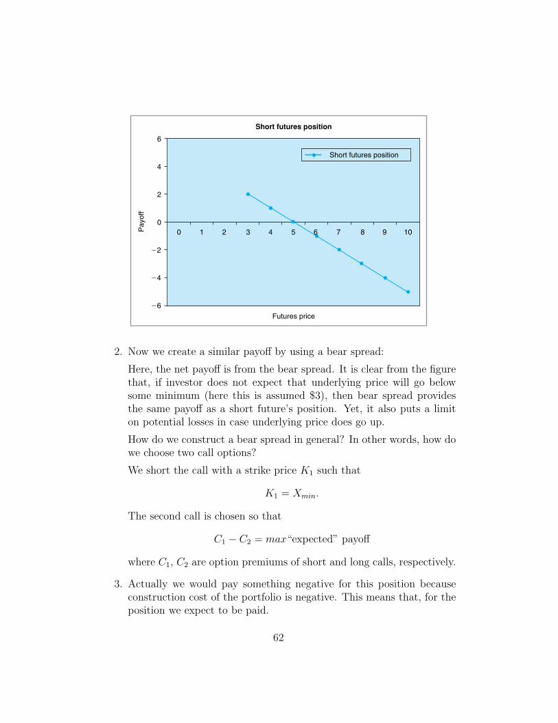
The pay off diagram for short futures position is given in 4a:

Short futures position

Short futures position

Futures price

Pay

off

6

4

2

00 1 2 3 4 5 7 8 9 10

22

24

26

6

Here, we assume that initial futures price is $5.

1. A bear spread can be created by buying a call option with strike priceof K1 and by selling a call option with a strike K2, such that K1 < K2.

Now assume that the investor does not expect a future’s price lessthan $3. Under this new assumption expected pay off diagram of shortfuture’s position would look like:

61

Short futures position

Short futures position

Futures price

Pay

off

6

4

2

00 1 2 3 4 5 7 8 9 10

22

24

26

6

2. Now we create a similar payoff by using a bear spread:

Here, the net payoff is from the bear spread. It is clear from the figurethat, if investor does not expect that underlying price will go belowsome minimum (here this is assumed $3), then bear spread providesthe same payoff as a short future’s position. Yet, it also puts a limiton potential losses in case underlying price does go up.

How do we construct a bear spread in general? In other words, how dowe choose two call options?

We short the call with a strike price K1 such that

K1 = Xmin.

The second call is chosen so that

C1 − C2 = max“expected” payoff

where C1, C2 are option premiums of short and long calls, respectively.

3. Actually we would pay something negative for this position becauseconstruction cost of the portfolio is negative. This means that, for theposition we expect to be paid.

62

Bear spread

Underlying price

Pay

off

6

4

2

00 1 2 3 4 5

22

24

26

Net payoff

Short call

Long call

6 7 8 9 10

This is because,

K1 < K2 ⇔ C1 > C2

4. Maximum gain = C1 − C2

Maximum loss = −C2.

5. See the Figure in part a.

Question 2

1. See the diagram below:

2. The quotations are in favor of euro calls which means that market isexpecting the value of euro to be higher which also makes euro callsmore valuable compared to euro puts.

3. It is clear that implied volatility for euro puts is less than the impliedvolatility for euro calls (See the text).

63

7.28

7.2 7.36

7.44

7.52 7.6 7.6

87.7

67.8

47.9

2

Payoff diagram for risk reversal

Euro exchange rate

Pay

off

0.1

0

0.2

0.3

0.4

0.5

Total payoff

Short put

20.1

20.2

20.3

20.4

20.5

Long call

4. These are the volatilities which must be plugged in (Black-Scholes)pricing formula to find the market price of options.

5. ATM volatility is the implied volatility which makes the market priceof an ATM option equal to price obtained from Black- Scholes formula.

Yes there are OTM vols as well. These may be different from the ATMvols, due to the presence of smiles or skews.

Question 3

1. See the Figure 10.20 in the text.

2. It is clear from this figure that this may be quite useful when a traderis betting on volatility movements. For example, if volatility has beenunusually high for a certain period of time, and an investor may thinkthat it may return to its “normal” level. Range binaries enable theinvestor to take positions on volatility. For a detailed explanation seethe text.

64

3. This may be the case if volatility is believed to be mean reverting, andif the current volatility is higher than its mean or alternatively duringthe holiday seasons.

4. Unexpected spikes in volatility can cause losses.

Question 4

1. See the Figure 10.20 in the text for range binaries. See also Figure 10.11for similarity between range binaries and short strangle positions.

2. When volatility is expected to be low, or when the underlying price isexpected to move in a certain range.

3. For butterfly structures see Figure 10.15 in the text. It is used to hedgelosses against unexpected spikes in volatility.

4. Risk arises from a short position on range binaries if volatility is highor if price moves in a very wide range.

5. This requires obtaining market data and then evaluating mark to mar-ket losses.

Question 5

1. They are all volatility positions. It is clear from the text that all threestructures have positive payoff if underlying price moves in a certainrange. Assuming that the volatility is low.

2. This is a static position (see the article in the question).

3. In the dynamic hedge, position makes money as underlying price fluc-tuates around the initial price. And this payoff increases as pricesfluctuations are more frequent. Similarly, pay off from (long) rangeaccrual options increases as long as price moves in a certain range.

4. By using dynamic hedging, a structure similar to range accruals can becreated.

65

Chapter 11

Pricing Tools in Financial Engineering

Exercises

Question 1

1. If there exist positive state prices, Q1, Q2, Q3 and Q4, which satisfy thefollowing matrix equation, then there are no arbitrage opportunities.

⎡⎢⎢⎣

10.910.860.77

⎤⎥⎥⎦ =

⎡⎢⎢⎣

1.113 1.113 1.092 1.0921 1 1 10.9 0.92 0.95 0.960.8 0.84 0.85 0.86

⎤⎥⎥⎦

⎡⎢⎢⎣

Q1Q2Q3Q4

⎤⎥⎥⎦

Solving the matrix equation above, we get:

⎡⎢⎢⎣

Q1Q2Q3Q4

⎤⎥⎥⎦ =

⎡⎢⎢⎣

−0.696190.9952381.55619

−0.94524

⎤⎥⎥⎦

2. As it can easily be seen, state prices, Q1 and Q4 are negative whichimplies that there are arbitrage opportunities in this market. However,such negative state-prices can result if the chosen model is incorrect.(If for example, the wrong number of states of the wrong set of assetsis chosen.)

3. 1X2 FRA rate is equal to current Libor rate of 5%. Remember thatcurrent time is t = 1, a 1X2 FRA starts (and expires) at time 1 andsettles at time 2 and finally the current Libor rate is 5%.

Question 2

1. Δ = 2005 = 40 days

or

Δ = 40365 = 0.1096 years.

66

By using equations (100)–(102), we can write:

u = eσ√

Δ

= e0.18√

0.1096

= 1.061

d = 0.942.

2.

p =erΔ −d

u − d=

e0.04x0.1096 − 0.9421.061 − 0.942

= 0.52

3. See the tree below for the binomial tree of stock price.

t = 0 t = 40 t = 80 t = 120 t = 160 t = 200

134.45126.72

119.44 119.37112.57 112.51

106.1 106.04 105.99100 99.95 99.89

94.2 94.15 94.188.74 88.69

83.59 83.5478.74

74.17

4. Using the binomial tree for stock prices in part d, we get the followingbinomial tree for the call premium:

67

t = 0 t = 40 t = 80 t = 120 t = 160 t = 200

34.4527.093

20.187 19.3714.349 12.891

9.813 8.156 5.996.505 4.99 3.101

2.981 1.605 00.831 0

0 00

0

Question 3

1. In this case where the stock pays continuous dividends of 4%, therewould be no changes in the binomial tree for the stock price. The treeis the same as in part (d) of the previous question. The only differenceis in the calculation of up-probabilities.

p =e(r−q)xΔ − d

u − d

=e(4%−4%)x0.1096 − 0.942

1.061 − 0.942

= 0.49

where, q is the continuous rate of dividends.

By using the binomial formula to determine the call premium, we get:

c = e−0.04(5x0.1096)5∑

i=0

Ci

(5i

)pi(1 − p)5−i

68

Where c is the option premium at time zero and Ci’s are the optionvalues on the expiration date for i = 5, C5 = 34.45, i = 4 and C4 =19.37, so on.

Computing the formula given above, we obtain, C0 = 5.53.

2. If stock pays 5% of its value as a dividend at the third node (t = 120days), this will result in the following binomial tree for the stock price:

t = 0 t = 40 t = 80 t = 120 t = 160 t = 200

127.73120.39

113.47 113.40112.57 106.89

106.1 100.74 100.69100 99.95 94.90

94.2 89.44 89.4088.74 84.26

79.41 79.3674.80

70.46

In order to compute call premium c at time zero, we can apply thebinomial formula in part (b) with:

p = 0.52

andC5 = 27.73, C4 = 13.40, C3 = 0.69

andC2 = C1 = C0 = 0.

The result is:c = 3.55.

3. See below for the binomial tree. The third type of dividend paymentcreates a non-recombining tree.

69

Question 4

1. Δ = 0.1096 years.

2. For this case we use equations (106)–(108), after adjusting them prop-erly:

u = e(r−rf)Δ− 12σ

2Δ + σ√

Δ

d = e(r−rf)Δ− 12σ2Δ−σ

√Δ

Then,u = 1.063

andd = 0.931, p = 0.5

3. Using the parameters in part one and two of this question, binomialtree for exchange-rate would be:

t = 0 t = 40 t = 80 t = 120 t = 160 t = 200

1.91.79

1.68 1.671.58 1.56

1.49 1.47 1.461.4 1.39 1.37

1.3 1.29 1.271.21 1.2

1.13 1.111.05

0.98

4. The binomial tree for European put will be given as in the next page.

5. The binomial tree for American (put) option is somewhat more com-plicated than that of the European (put) option. The reason for thatis that American options can be exercised earlier.

70

t = 0 t = 40 t = 80 t = 120 t = 160 t = 200

00

0.01 00.031 0.02

0.065 0.052 0.040.11 0.099 0.085

0.156 0.147 0.130.213 0.209

0.281 0.290.354

0.42

At each node, value of an American option is equal to its intrinsic valueor to the value which comes from holding it until next time (node)whichever is greater.

This gives the binomial tree for the American put option, where thevalues are calculated backwards. The tree is shown below.

Question 5

1. Applying equations (100)–(102), we determine u = 1.10, d = 0.91 andp = 0.51.

2. We can directly apply the binomial formula to determine the value ofthe call option. Alternatively we can use binomial tree methods. Bothwill lead to the same answer:

C = $5.50

3. For the barrier option, it is instructive to have a look at the binomialtree. The value of the barrier call option along the paths which lead to$120 stock price becomes zero. In this case call premium will be:

Cb = $0.041.

71

t = 0 t = 40 t = 80 t = 120 t = 160 t = 200

max(−.50,0)max(−.29,0)

max(−.18,.01) max(−.27,0)max(−.08,.04) max(−.06,.02)

max(.01,.09) max(.03,.07) max(.04,.04)max(−.10,.15) max(.11,.14) max(.13,.08)

max(.20,.21) max(.21,.21) max(.13,.13)max(.29,.29) max(.3,.21)

max(.37,.37) max(.29,.29)max(.45,.35)

max(.42,.42)

4. Barrier option will be cheaper.

72

Chapter 12

Some applications of the Fundamental Theorem

Exercises

Question 1

1. In this exercise, we can easily employ the equations (66)–(70), (79)–(80)and (82)–(86). Also, remember that BDT model will yield a recombin-ing binomial tree.

2. Using the equation,

EP [Li] =B(0, i)

B(0, i + 1)− 1

we get:

L0 = 5.26%

EP [L1] = 2.15%

EP [L2] = 2.20%

EP [L3] = 2.25%.

Also,EP [L1] = 0.5x(Lu

1 + Ld1)

andLu

1 = e2σ1Ld1.

Solving these two equations, we find

Lu1 = 2.58%

andLd

1 = 1.73%

We can use the same logic to determine all possible values of the Libor ratesat each node. This would lead to the following values:

73

At node 2:Luu

2 = 3.42%Lud

2 = Ldu2 = 2.07%

Ldd2 = 1.26%

At node 3:Luuu

3 = 3.84%Luud

3 = Ludu3 = Lduu

3 = 2.58%Ludd

3 = Ldud3 = Lddu

3 = 1.73%Lddd

3 = 1.16%

1. BDT tree for bond price of B(0,4) can be found by using the libor ratesdetermined in the previous part (a): In the following figure, at eachnode, the numbers in the top box refer to money market account, andthe numbers in the second box refer to price of bond at this node.

Forward price of bond which expires at time 4, at node 2 is the expectedprice of this bond at node 2. So forward price would be 0.5(94.80 +96.63) = 95.72.

Node 1 Node 2 Node 3 Node 4

1.1166

1.1595

1.1454

1.1304

1.1210

1.118

1.1031

1.0969

100

100

100

100

100

100

100

1.1020

1.0929

1.0843

97.89

97.89

98.57

96.89

1.0797

1.0708

1.526

89

$1

93.70

94.80

96.63

Node 0

74

2. Price of the call option which expires at time can be calculated fromthe binomial tree presented below:

94.80

93.7089

C 51.80

C52.63

C53.63

96.63

C52.53

Question 2

1.LUS =

100B(t, t + 1)US

− 1 = 1.08%

and

LEuro =100

B(t, t + 1)Euro− 1 = 1.29%

2.rUSt = log(1.108) = 1.074%

and

rEurot = log(1.0129) = 1.28%.

75

3. We need to use continuously compounded rates.

4. Forward Libor model uses Libor rates.

Question 3

1. Consider the Stochastic Differential Equation,

St+Δ = St + (r − rf )StΔ + σSt+Δ

√Δet+Δ

and the time interval,Δ = 1

2. Assume that the following sets of random numbers are given:

{−0.4326, −1.6656, 0.1253, 0.28779, −1.1465}

{1.1909, 1.1892, −0.0376, 0.3273, 0.1746}{−0.1867, 0.7258, −0.583, 2.1832, −0.1364}{0.1139, 1.0668, 0.0593, −0.0956, −0.8323}{0.2944, −1.3362, 0.7143, 1.6236, −0.6918}.

These five trajectories are risk free since, i) random variables in eachset have a mean of zero and ii) the equation given in part (a) has aknown mean that equals interest rate differentials.

We can compute the exchange rate, Sji ,where j is the path index and

i is the node (time) index. (Remember that the Δ = 1 otherwise, thedrift of the equation below will involve a Δ as well.)

Sji = Sj

i−1 + (r − rf )Sji−1 + σSj

i−1eji .

For example,

S11 = S0(1+r−rf +σe1

1) = 1.1015(1+0.01074−0.0128+0.15x(−0.4326)

= 1.0278

76

Similarly we can compute the remaining values for path one:

S12 = 0.7689, S1

3 = 0.7818, S14 = 0.8140, S1

5 = 0.6724

Path 2:

S21 = 1.2961, S2

2 = 1.5247, S23 = 1.5130, S2

4 = 1.5843, S25 = 1.6226

Path 4:

S41 = 1.1181, S4

2 = 1.2948, S43 = 1.3037, S4

4 = 1.2824, S45 = 1.1198

Path 5:

S51 = 1.1479, S5

2 = 0.9156, S53 = 1.0118, S5

4 = 1.2562, S55 = 1.1234

3. Assume that we are dealing with a put option. Then, by simply check-ing the third number in each path, we can determine the value of theoption at expiration.

Finding the expected value of the option at expiration and discountingit we get

P = 0.0319

(Remember that each path has a probability of 0.2.)

Question 4

1. By using the parameters provided in the exercise and the methodemployed in the previous question, we proceed as follows:

(a) We assume three time steps which implies that Δ = 90 days.We generated the following 5 set of random numbers:Set 1: {0.9501, 0.7621, 0.6154},Set 2: {0.2311, −0.4565, 0.7919},Set 3: {0.6068, 0.0185, −0.9218}Set 4: {−0.4860, −0.8214, 0.7382},Set 5: {0.8913, 0.4447, −0.1763}.

77

The values of exchange rate, on each of 5 paths, will be:Path 1:

S11 = 4.1532, S1

2 = 4.5216, S13 = 4.8564

Path 2:S2

1 = 3.8835, S22 = 3.7548, S2

3 = 4.0991

Path 3:S3

1 = 4.02144, S32 = 4.0822, S3

3 = 3.7569

Path 4:S4

1 = 3.6146, S42 = 3.3629, S4

3 = 3.6532

Path 5:S5

1 = 4.1311, S52 = 4.3665, S5

3 = 4.3441

Let’s assume that the option under consideration is a call optionwith an exercise price of 4.10Peso/$.It is easy to see that call option expires in the money only in paths1 and 5. So, we first compute the value of the option on each path,determine its expected value and then discount it with Mexicaninterest rate.Hence, the call premium is 0.1884.

2. This information is important in a sense that it is an additional riskfactor which affects the exchange rate process.

3. Let’s first have look at the distribution of the reserves. Let Rt be thelevel of reserves. Then the distribution of log(Rt)is

φ[log(R0) + (μ − σ2

2)T, σ

√T .

So probability that Rt < 6 (probability of experiencing a one shot de-valuation) is less than 2%. Even though the information is importantin pricing the option, it is very hard to determine its effect when weuse only 5 paths with only 3 steps.

So we need to increase the number of paths and steps to allow for suchan event with very low probability. We can proceed in two ways. Either

78

we can use the same random variables generated for the exchange rateprocess to compute the reserves.

Here we assume that there is a perfect correlation between two pro-cesses. Or, alternatively, we can generate a separate set of randomvariables which implies that there is no correlation between the two.

79

Chapter 13

Fixed Income Engineering

Exercises

Question 1

1. In order to compute the bond prices from FRA rates, we can simplyuse the equation (23) in the chapter.

B(t0, ti) =100

i−1∏j=0

(1 + δF (t0, tj))

whereδ = 0.25 years

and F (t0, ti) is the i × (i + 1) FRA rate.

Using the equation we will get the following discount bond prices:

Term Bid Ask3 99.01 99.016 97.88 97.919 96.72 96.7712 95.51 95.5815 94.16 94.2818 92.70 92.86

2. We use the following relationship between discount bond prices and theyield:

B(t0, ti) =100

1 + δiri

where δi is the time to maturity as a fraction of a year, and ri is thecorresponding interest rate (yield) for that maturity.

80

Rewriting the equation in terms of ri, we get

ri =1δi

(100

B(t0, ti)− 1

)

Using this equation we obtain the yields shown in the first Table below.

Yield CurveTerm Bid Ask3 4.00 4.006 4.27 4.329 4.45 4.5212 4.63 4.7115 4.85 4.9618 5.12 5.25

3. Computation of swap rates is explicitly shown in the text. We canapply equations (25)–(31). This would yield the swap curve which isshown in the second Table below

Swap CurveTerm Bid Ask6 4.50 4.609 4.60 4.7012 4.73 4.8315 4.92 5.0418 5.15 5.29

4. We can easily see that curves computed in part (1) and (3) are not thesame. The following graph shows this:

5. See appendix for the calculation of the par yield curve. We can derive

yn =1δ

⎛⎜⎜⎝100 − B(0, n)

n∑i=1

B(0, i)

⎞⎟⎟⎠

81

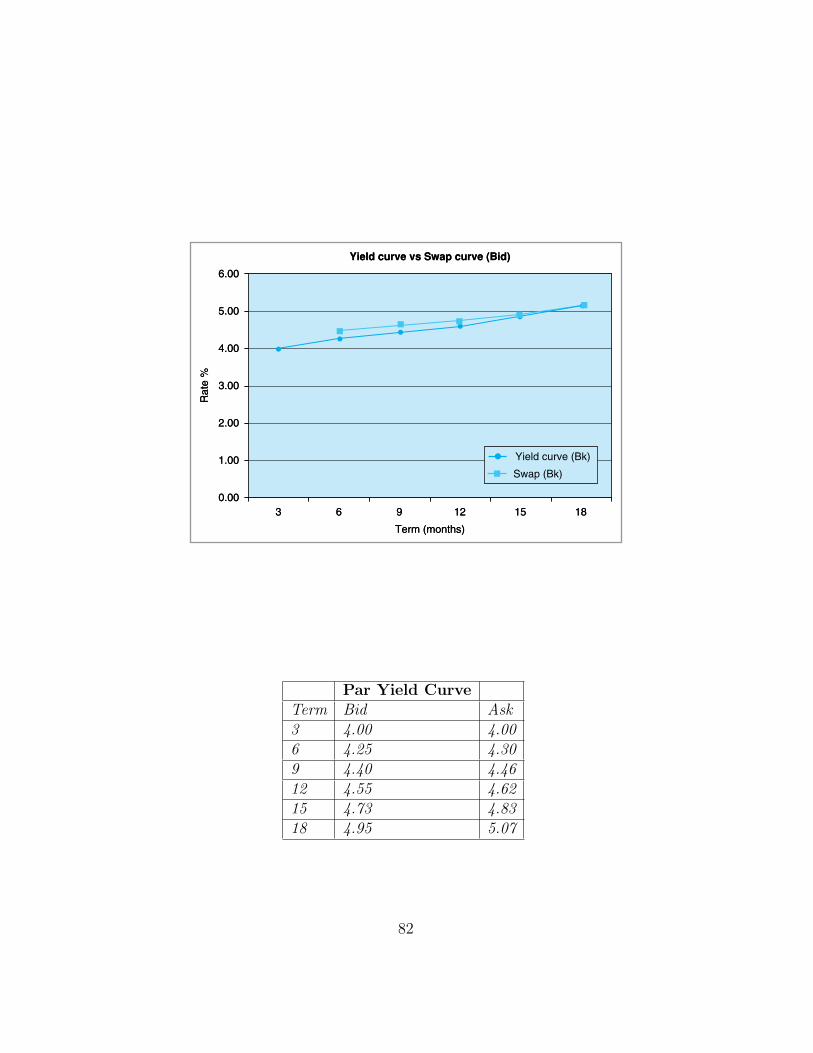
6.00

Yield curve vs Swap curve (Bid)

5.00

4.00

3.00

Rat

e %

2.00

1.00

0.003 6 9 12

Term (months)

Yield curve (Bk)

Swap (Bk)

15 18

6.00

Yield curve vs Swap curve (Bid)

5.00

4.00

3.00

Rat

e %

2.00

1.00

0.003 6 9 12

Term (months)

Yield curve (Bk)

Swap (Bk)

15 18

Par Yield CurveTerm Bid Ask3 4.00 4.006 4.25 4.309 4.40 4.4612 4.55 4.6215 4.73 4.8318 4.95 5.07

82

from the equation provided in the appendix (δ = 0.25 years).

This leads to:

6. The computation of zero-coupon yield curve is very similar to compu-tation of yield curve from discount bond except that the yield this timecorresponds to a formula that uses Bond-equivalent yields:

B(t0, ti) =100

(1 + yi)δi

where δi is the same as in part (2). Solving this equation for yi, weobtain:

yi =

((100

B(t0, ti)

) 1δi

− 1

).

By using the formula just derived, the zero coupon rates are computedas in the Table below.

(You may, alternatively, follow the method described in the Appendixto calculate the zero-coupon yield curve from par yield curve).

Zero-Coupon Yield CurveTerm Bid Ask3 4.06 4.066 4.37 4.329 4.54 4.4712 4.71 4.6315 4.93 4.8218 5.18 5.06

Question 2

1. Let’s start by considering the following two portfolios:

Portfolio A: Nominal = $100. Long position in (0 × 1) and (1 × 2)FRA’s.

Portfolio B: Nominal = $100. Long position in plain vanilla swap.

83

Portfolio A:

Since we start at time zero, we already know the current Libor rate L0

and (0 × 1) FRA rate. They are both equal to 5%. But, we do notknow L1 and the (1 × 2) FRA rate.

L0L1

?

F132

5%

5%

Portfolio B:

L0L1

?

F132

5%

5%

From the text we know that both structures are very similar to eachother. We can use that similarity to derive the (1×2) FRA rate. Indeed,we have the following relationship between FRA and swap rate: (Seeequation (17) and explain why we can’t use it)

84

$100(

5%1.05

+F1x2

(1.05)(1 + F1x2)

)= $100

(6.2%1.05

+6.2%

(1.05)(1 + F1x2)

)

Simplifying and rearranging:

F1x2 =6.2% + (6.2% − 5%)

1 − (6.2% − 5%)= 7.49%

In order to write a general formula, it would be helpful to write thesame equation for F2x3.

F2x3 =6.4% + (6.4% − 5%)x(1.0749) + (6.4% − 7.49%)1 − ((6.4% − 5%)x(1.0749) + (6.4% − 7.49%))

= 6.84%

Then a general formula would be in the form of:

F(n−1)x(n) =Sn +

n−1∑i=1

[(Sn − F(i−1)xi)n−1∏

j=i+1(1 + F(j−1)xj)]

1 −n−1∑i=1

[(Sn − F(i−1)xi)n−1∏

j=i+1(1 + F(j−1)xj)]

Using the general formula just derived, we obtain the following FRArates (We used bid quotations for the corresponding swap rate):

Term FRA0X1 5.001X2 7.492X3 6.843X4 9.114X5 9.985X6 12.11

After computing the FRA rates from swap curve, the rest is relativelyeasy to handle.

85

Term Bond Price1 95.242 88.603 82.934 76.015 69.116 61.64

2. We can follow the same method used in the previous question part (1).As a result we get the answers shown in the Table below.

3. See question one, part (2) for the details:

Term Yield1 5.002 6.433 6.864 7.895 8.946 10.37

4. See the previous question, part (5):

Term Par Yield Curve1 5.002 6.203 6.404 7.005 7.506 8.10

86

Question 3

1. The bid-ask spread on a forward start swap is equal to Sask −Sbid. Wecan use the equations (25)–(31) to compute Sask and Sbid.

Sbid2×5 =

B(0, 3) × F2×3 + B(0, 4)F3×4 + B(0, 5)F4×5

B(0, 3) + B(0, 4) + B(0, 5)

=82.93 × 6.84% + 76.01 × 9.11% + 69.11 × 9.98%

82.93 + 76.01 + 69.11= 8.55%

The Sask can be computed in a similar way.

2. The price of the coupon bond at time zero is given by

P (0, 4) =

(4∑

i=1

B(0, i) × $7

)+ B(0, 4) × $100

= $100.

A trader who wants to (forward) sell this coupon bond at a price of F ,to be delivered at time 2, may want to hedge himself. So this tradercan buy this coupon bond in the spot market today and “store” it.Since its price is $100, he needs to borrow $100 for funding purposes.

When the trader receives coupon payments at time 1 and 2 and theforward price amount, F of the coupon bond, the trader will repay theinitial $100. This means that the trader needs to borrow:

B(0, 1) × $7 + B(0, 2) × ($7 + F ) = $100.

Solving this equation we find,

F = $98.34

87

Chapter 14Tools for Volatility Engineering, Volatility Swaps, and

Volatility Trading

Exercises

Question 1

1. Let’s look at the cash flow of the volatility (variance) spread swap:

−(σ2Nasdaq − σ2

S&P500)N2

It is clear from this expression that investor actually takes a longposition on the S&P500 variance and a short position on the NASDAQvariance. This trade can be put in place by simultaneously entering intoa long S&P500 variance swap and a short NASDAQ variance swap.

Pricing here is to determine the initial variance swap spread whichmakes the initial value of the swap between the two indices have avalue of zero. This price is given as 21% in the question.

2. Yes, we need the correlation between the two markets.

If the correlation is high (close to one in absolute value) between thesemarkets, then this implies that most of the time, volatility will movein both markets in the same direction which in return, indicates thatvolatility (variance) spread is relatively tight in the long run (Thismakes the position mentioned in the question reasonable). So the fixedleg of the spread has to be set (relatively) higher.

If the correlation is low (close to zero in absolute value), which impliesthat these two markets move more or less independently from eachother, then there is no reason to believe that the volatility spreadbetween the markets should get narrower.

It is less likely that the investor who holds a long position will end upwith a positive payoff. In order to make the initial value of the swapequal to zero, the fixed leg of the spread needs to be set at a lower level.

3. The smile effect is important. However, in this present case the tradeconcerns realized volatility and not the Black-Scholes implied volatility.This means that the pricing of the swap will make no use of the smilein any direct way. Indirectly, the smile can be useful to calibrate amodel, on the other hand.

88

4. If the position is taken by using volatility (variance) swaps, then thismay be less risky compared to the other ways of taking the same posi-tion. Also the pricing of the instrument may be easier. (See the exercisefor alternative ways of taking the same position and see the text forthe risk of these positions).

The main risk involved here is related to the assumption that the long-run dynamics of the volatility spread is stationary. If this underlyingassumption is violated, then the position may lose.

Question 2

1. If an investor buys long-dated volatility, and sells short-dated volatil-ity,then the investor is expecting a decrease in the short dated volatilityand an increase in the long dated volatility.

Of course, there is no guarantee that these expectations will be realized.If short run volatility goes up or / and long run volatility decreases,the pay off from the position would definitely be negative.

2. This is equivalent to an investor constructing a short straddle positionby using knock-out options. Long straddle may be constructed by usingoptions which have break-out clause to put a limit to unrestricted riskof loss that arises from the short (straddle) position in the short run.

If short dated volatility turns out to be high, an additional premiumcan be triggered on the options which are used for the long straddle.This additional payoff from the long volatility position off sets the lossesfrom the short volatility position.

3. The relevant payoff function will shift upwards by the amount of theadditional payoff.

4. If the additional premium is a fixed amount, this may cut potentiallosses, yet it may not be sufficient enough. However, considering thatthe short position is taken for one month, this risk may not be a verybig risk.

5. It is clear from the text (see section 3.3) that volatility positions takenby using the straddles are not pure volatility positions.

89

Chapter 15

Smile Effects in Financial Engineering

Exercises

Question 1

1. In this question the implied volatilities are computed by using a risk-free interest rate of 2%. The calculations are summarized by the fol-lowing figure.

0.50

0.45

0.40

0.35

0.30

0.25

0.20Vol

atili

ty

0.15

0.10

0.05

0.00

K/S

Vol_bkl

Vol_ask

Volatility smile put-bid/ask

0.68

0.76

0.81

0.88

0.92

0.95

0.98

2. The calculations yield the following results in the Figure shown below.

The bid-ask spread on the implied volatilities can be seen in the fol-lowing Figure. Clearly, these spreads are not constant across optionswith different moneyness.

90

0.25

0.20

0.15

0.10Vol

atili

ty

0.05

0.001.02 1.04 1.04 1.05 1.07

Call volatility smile-ask

K/S

Vol_ask

1.09 1.10 1.12 1.15 1.19

3. When the two Figure are put together the result will be more like askew.

91

0.50

0.45

0.40

0.35

0.30

0.25

0.20

0.15

Vol

atili

ty

0.10

0.05

0.00

K /S

Vol_ask

Vol_ask (put-call)

0.750.81

0.880.92

0.950.98

1.021.04

1.071.10

1.150.68

Question 2

1. Cap/floor volatility is thought to be higher than swaption volatilitybecause, the market buys volatility trough swaptions and sells volatil-ity trough cap/floors. Everything else being the same the bid-ask dif-ference should make cap/floor volatility a little higher.

(a) A callable bond has a higher coupon because the bond incorpo-rates a short swaption. If rates fall below a level, the issuer hasthe right to call the bond at par. From bondholder’s point of viewthis is equivalent to selling a swaption. The option holder has theright to get into a fixed receiver swap that pays the same couponat the call date.This embedded option will have a premium and this premiumwill make the coupon of the callable bond higher. Investors mayconsider these higher coupons as yield enhancement and buy thesebonds. (Callable bonds are usually not callable for a certain periodafter the issue date. During this period the investor will receivethe high coupon regardless of the interest rate movements.)

92

(b) On the other hand caps/floors are used by corporates to hedgethe interest rate risk. So, the market will structurally be shortcaps/floors but long swaptions.

2. Market sells financial services to corporates. One of these services ishelping them hedge interest rate risk. This is done using caps andfloors.

On the other hand, market sells yield enhancement products toinvestors. These structures are often callable, which results in theembedded swaption.

3. This statement is an example of hedging and risk managing of volatil-ity risk. The industry is buying and selling volatilities and meetingdifferent needs of its clients. However, the two risks are not identicaland the “volatility books” need to be carefully managed in order to beproperly hedged.

Also, note that from the point of view of a volatility trader the samerisk can be hedged in (many) different ways and by using differentfinancial instruments. Some alternatives can be cheaper than others.

93

Chapter 16

How do Credit Derivatives Change Financial Engineering?

Exercises

Question 1

1. The standard approach here is to calculate some conventional ratios.These ratios can then be used along with regression analysis to estimatethe default probability.

2. To obtain the migration matrix for a particular credit rating, oncecould look at the past ratings data on all corporates and calculate thestatistical estimates for the transition probabilities from one rating toanother in a given time period.

3. There are many credit ratings and each credit comes with a migrationmatrix. Using past data one can also calculate the joint probabilitiesthat two or more credits migrate to a different rating.

Question 2

1. See figure 5.6 and the related example in section 3.2.1 in the text.

2. See figure 5.5 and the related example in section 3.2 in the text.

3. Yes, a swaption will be needed. The main reason being that Bond A iscallable after 3 years and matures in 4 years whereas Bond B matures in5 years. It is clear that if interest rates decrease substantially, Bond Awill be called.

4. First, let’s look at the required structure to convert Bond A in toBond B:

(a) To eliminate the credit risk involved in Bond A, we need to buya CDS with 4 year maturity. That will change the credit of theinitial portfolio from AA- to AAA.

94

(b) Second step involves the conversion of fixed rate in to floating rate.For this we need a (fixed payer) interest rate swap in USD withmaturity 5 years.

(c) By using a cross currency swap (floating to floating), we exchangeUSD floating into DEM floating. So we need a currency swap for5 years.

(d) Finally, we need to hedge the risk mentioned in part (c). So weshould buy a (Bermudan type) swaption in USD.

Question 3

(a) A typical cash flow diagram will incorporate the following.If you are short the CDO, then you receive a fixed amount atthe initial point to. Then you make payments made of a floatingrisk-free rate plus a fixed spread. However, if one or more of theunderlying credits default your share of the defaulted amount willbe deducted from the coupon.

(b) Since you are receiving a spread over a floating rate, the interestrate risk is minimal. There is some risk only between the couponpayments dates. This can be hedged using strips of FRA’s. Or,by using swaps as the reading suggests.Otherwise the CDO is an investment vehicle and the investor isexposed to changes in the credit curve. If needed, such risks canbe hedged by taking positions on a proper set of CDSs.

(c) A decline of the overall level of interest rates means the floatingrates are going down. If the investor is hedged trough the FRA’sthis will have no effect on the overall returns. On the other handif default rates increase the value of the CDO will decline.

(d) As underlying credits default this will decrease the principalamount involved in the CDO during its life cycle. On the otherhand if such a CDO is hedged using a swap, the swap notionalwill remain fixed.

95

This means that a plain vanilla swap will end up introducing abasis risk. However, a customized swap where the swap notionaldecreases as CDO principal changes will be more expensive.

96

Chapter 16

Credit Markets: CDS Engineering

1. Written in edition 1.

2. Written in edition 1.

3. Written in edition 1.

4. (a) i. The following figure shows the cash flows involved in the trade.

t0 t1 t2 t3 t4 t5

N

Ct0

Ct0

ct0

ct0

N

N

ii. Clearly a negative basis trade is going on, leading to a risk-free gain. ING claims that while CDS rate ct0 has decreasedby 5bps, Attentat 2010 bond price has increased 1bp recentlywhich is an anomaly. So, according to ING the CDS rateshould eventually increase leading to gains from the currenttrade.

iii. The bond is bought for 100 which pays fixed coupons Ct0 ateach time point if it doesn’t default. But it is default protectedthrough the CDS by a payment of midas+27bp. The expectedreturn is Ct0 − ct0 at each coupon payment date. (Assumingthat the insurer does not default.)

iv. There might have been a surge of structured produce likeCDOs being issued in the market which narrowed the CDSspread where as the bond spread has actually increased.

97

(b) The LBBW is granfathered and hence is guaranteed to providethe said returns on the holding. So if a trade neutral position isheld by being short in DG Hyp 4.25% and long in LBBW 3.5%(under swaps), as spreads tightens, the gains from LBBW willremain the same but the payments for being short in DG Hyp willdecline leading to eventual gains from holding this position.

Receive (Libor 1 6.5bp) N

Pay 4.25%Nt1

Pay (Libor 1 4.2bp)M

Receive 3.5% M

t1

In the second case Land Berlin 2.75% is risk protected and hencethe same logic as the previous case holds.

Receive (Libor 1 5.4bp) N

Pay 3%Nt1

Pay (Libor 1 2.7bp) M

Receive 2.75% M

t1

(c) Note that the trade has an yearly positive carry. Besides the5-year iTraxx spread 38bp is considered to be high now, consid-ering the forward rates. Hence they are expected to drop in thefuture. Thus this trade results in an advantage for the investorif implied forward rates are higher than they should be. Observethe graph below.

98

Time(in years)

Spr

ead

3 10

20.75bp

38bp

61.25bp

5

99

Chapter 16

Case Study: Credit-Linked Notes

(a) Credit linked notes are assets issued by financial institutions whichhave exposure to the credit risk of a reference Issuer. These notespay an enhanced rate to the investor for taking on this addi-tional credit risk. If the Reference Issuer defaults then the investorreceive the recovery price of the reference security.Most credit linked notes are issued as traditional medium termnotes that contain embedded credit default swaps.Example:Drug company Credit Linked NoteTermination Date: 5 YearsReference Security: ABC bond 7.125% maturing 12/1/09Interest: Libor + 50bp per annum. Interest paid quarterly.In this CLN the investor receives Libor + 50bp coupon against theexposure to the default risk of the drug company in an asset backedtrust.Thus a CLN will be preferable to a straight Treasury if the investordesires a higher coupon associated with the risk of default of acertain security.

(b) Investment banks may need to hedge their position during theissuance process as the readings suggest. The process of packaging,pricing and selling a CLN may take time and during this periodmarkets may move.As dealers issue CLNs they will have short derivatives positionsmentioned in the text, in particular they will have short CDspositions.

(c) In the text the climate has been influenced by a shortage of cor-porate bonds in the secondary market.Note that when this happens the value of these bonds would go upand the associated “risk premium” would decline. As discussed inChapter 16, this would lead to a lowering of the associated CDSrate.

100

(d) The arbitrage mentioned in this reading is in fact a true arbitragein the academic sense. The logic of the arbitrage argument goesas follows.A basket of corporate bonds is something similar to a syntheticCLN packaged using the same names by a dealer. They both haveexposure to an identical set of credits, they contain very similardefault risks and they pay an enhanced coupon. Hence in theorythe difference between the coupon paid by the basket and thesynthetic CLN should be the same.Yet, as discussed in the chapter technical factors may make the twocoupon diverge from each other. This is called the bond basis. Thetext mentions that this basis was negative originally and becameeven more negative as a result of the activity mentioned in thereading.Those dealers who had access to the underlying bonds could thenput together packages, by selling and buying the underlying andthe associated CLN.To represent the cash flows in a graphic one would use Figure 16-5and put it together with the cash flows of a risky bond, which willbe similar.

(e) If some bonds become special in the repo market, this means thatthere is a great deal of demand for them. Under such conditionsthose players who want to borrow these bonds will be willing to“surrender” their cash to the repo dealer at zero interest.

(f) Because if they have the bonds in their portfolio they give to bondto repo dealer and receive cash at zero cost, instead of payinginterest to banks.

101

Chapter 17

Essentials of Structured Product Engineering

1. (a) Let rm denote the m month swap rate (or Libor rate). Then the3 × n month forward rate f(3×n) is calculated thus:

(1 + r3312

)(1 + f(3×n)n − 3

12) = (1 + rn × n

12).

The discount curve is calculated thus : the n- month discount rateB(t0, tn) is

B(t0, tn) =1

n−1∏i=0

(1 + ri/12).

(b) The 24 × n month forward rate f(3×n) is calculated thus:

(1 + r3

2412

)(1 + f(24×n)

n − 2412

)= (1 + rn × n

12).

(c) The components for this note is a discount curve, a 2-year forwardcurve, a market for CMS swaps and Bermuda swaptions (since thenote is callable).

(d) Let cmsj,ki denote j-year CMS bought for k years evaluated at the

i-th year. Let ct0 be the premium for a 2-year Bermuda swaption.Calculate R1 = L0 + α0, where L0 is the current 1-year Libor rateand α0 is calculated as:

ct0 = α0 + B(t0, t1)α0 + B(t0, t2)α0.

Year 2 coupon is: α1(cms2,32 )+L0+α0. We know cms2,3

2 and henceα1 is calculated by equating:

α1(cms2,32 ) + L0 = cms2,3

2

giving α1 = 1 − L0

cms2,32

. Similarly α2 is calculated from

α1(cms2,32 ) + α2(cms2,3

3 ) + L0 = cms2,33

giving α2 = 1 − cms2,32

cms2,33

.

102

(e) The components for this note is a discount curve, a 3-year anda 2-year forward curve, a market for CMS swaps and Bermudaswaptions(since the note is callable).

(f) Let ct0 be the premium for a 2-year Bermuda swaption. CalculateR1 = L0 + α0, where L0 is the current 1-year Libor rate and α0 iscalculated as:

ct0 = α0 + B(t0, t1)β1 + B(t0, t2)β2.

Here ct0 , B(t0, t1), B(t0, t2) are known and the rest α0, β1, β2 hasto be determined from that. α is calculated as α = cms3,3

0 −cms2,30

s30

where s30 is the 3-year swap rate.

(g) β1 = β2 can be chosen appropriately to satisfy ct0 = α0+B(t0, t1)β1

+B(t0, t2)β2.

2. (a) The note can be engineered thus:

• 1-year Libor deposit.• Get into a receiver interest rate swap paying Libor and getting

5.23%.• Buy digital cap (for Libor > 6.13%) and digital floor (for

Libor > 6.13%).• Pay CMS10 for first 2 years and 8 × CMS10 for the next

three years.• Receive CMS30 for first 2 years and 8×CMS30 for the next

three years.

(b) An investor who expects the yield curve to steepen in the longrun and expects Libor to remain quite high would demand thisproduct. She/he would expect Libor to increase and also theCMS spread to increase leading to an increase in the differenceCMS30 − CMS10.

3. (a) The investor expects that the CMS10 rate would graduallyincrease.

(b) If the CMS10 curve flattens or the rate does not increase signifi-cantly (slow increase) then the coupons will go on decreasing andmight become negligible.

103

The other risk is that the issuer might not call the note in such asituation and the investment would be stuck having sub-optimalgains.

(c) (typo in problem, should be CMS10 instead of Libor, and we havean additional rate 10% ) The following table give the coupons,given that we know the CMS rates as given in the problem:

Y ear1, Q1 : 9.00%.Y ear1, Q2 : (9.00 + 5.00 − 4.65)% = 9.35%Y ear1, Q3 : (9.35 + 6.00 − 4.85)% = 10.50%Y ear1, Q4 : (10.50 + 6.50 − 5.25)% = 11.75%Y ear2, Q1 : (11.75 + 7.00 − 5.45)% = 13.30%Y ear2, Q2 : (13.30 + 8.0 − 5.65)% = 15.65%Y ear2, Q3 : (15.65 + 9.0 − 5.65)% = 19.00%Y ear2, Q4 : (19.00 + 10.0 − 5.65)% = 23.35%Y ear3 : (23.35 + 10.0 − 5.65)% = 27.70%Y ear4 − 10 : (23.35 + 10.0 − 5.65)% = 27.70%

So, as the CMS10 rate increases the coupon payment snowballs.The following table give the coupons, given that we know the CMSrates are constant at 3.5% as given in the problem:

Y ear1, Q1 : 9.00%.Y ear1, Q2 : (9.00 + 3.50 − 4.65)% = 7.85%Y ear1, Q3 : (7.85 + 3.50 − 4.85)% = 6.50%Y ear1, Q4 : (6.50 + 3.50 − 5.25)% = 4.85%Y ear2, Q1 : (4.85 + 3.50 − 5.45)% = 2.90%Y ear2, Q2 : (2.90 + 3.50 − 5.65)% = 0.75%Y ear2, Q3 : max(0.75 + 3.50 − 5.65, 0)% = 0%Y ear2, Q4 : 0%Y ear3 : 0%Y ear4 − 10 : 0%

Since the CMS10 does not increase, the coupon value decreasesand reaches 0%.

(d) This coupon can be characterized by an interest rate swap. Notethat the CMS10 rates are all known. Hence the coupons are allfixed in the beginning. The investor can pay the fixed couponsand receive Libor at every coupon payment date.

104

(e) If the 8 FRAs are known, we can calculate the discount curve fromthat. Now if the coupons at each time ti is cti , then the price ofthe coupon at ti is

Pi = B(t0, ti)(cti − Fti)

where Fti is the forward rate at ti.

(f) The first years coupon is generated from Libor and a part of theprice of the Bermuda swaption sold.

(g) The coupons are floored as mentioned (“minimum of 0%”)

(h) CONTRACTUAL EQUATION:Snowball Note = Libor deposit + Receiver interest rateswap (wrt CMS10) + Short Bermuda swaption

4. The CMS spread note can be engineered thus:

• Deposit $10 million earning Libor.

• Get into a 10 year Receiver swap.

• Receive 16×CMS30 and Pay 16×CMS10 for 10 years with twoCMS swaps.

• Sell a Bermuda swaption.

• Buy a CMS spread floor and a CMS cap.

(a) The investor expects the yield curve will steepen in the long run.

(b) The obvious risk is if the yield curve flattens then there will bevery low yielding coupons. Also the coupon may not be calledwhile a low yield is going on. Of less significance but still to beremembered is that in case of very steep yield curve, the gains willstill be capped at 30%.

5. (a) This coupon can be engineered with the help of knock-in andknock-out put options.

(b) This product does depend on forward volatility since the pricingand hedging of these options are dependent on volatility.

105

Chapter 18

Credit Indices and their Tranches

1. (a) A barbell is a strategy of maintaining a portfolio of securities con-centrated at two extremes in terms of maturity date: very short-term and very long term.A positive roll down is a positive return from a security tradingat a discount which reaches its par value near the maturity date.Time decay is the ratio of the price with respect to a decreasein time to expiration of any asset whose value decreases overtime.

(b) A jump to default occurs when an investment grade entity withhigh rating which has been continuing in subsequent rolls of acredit index without degradation (in credit rating) suddenlydefaults.

(c) SG’s strategy: Since the 7-year equity correlation has tightened,the spread has increased against the 5-year and 10-year spreads.Hence it is profitable to sell the 7-year equity tranche protectionand buy the 5-year and 10-year equity tranche protection barbell.Naturally there is a steepening of the 7−year spread. A jump todefault is well protected by the 10-year protection.SG thinks that Alstom’s 3-5 year curve is steep. This meansAlstom March 2010 bonds at 6.25% would lead to mark-to-marketgains. The 3 − year CDS provides the protection against default.

2. (a) Suppose we have a portfolio of n names with some default corre-lation ρ. The risk of the entire portfolio moves according to thechange in default correlation. On the other hand if the portfo-lio is tranched according to the order of their defaults then thevarious tranches behave differently as ρ changes. For example,a high ρ indicates subsequent defaults occurring together whereas a low ρ makes occurrence of subsequent defaults more or lessindependent.

(b) As default correlation increases the area under the middle partof the default density function decreases and the mass on thetwo extreme tranches increase. Hence area under the subordinate

106

tranche increases, which means that the probability that the sub-ordinate tranche loses all its money decreases. Hence the risk forthis tranche decreases along with the spread.On the other hand the cushion for the senior tranches decrease asdefault correlation increases. Hence it is more likely that the theprotection seller for the senior tranches will concede some losses.Hence the risk and hence the spread for this tranche increases.

(c) With a decrease in default correlation one should long on protec-tion on the subordinate tranches and short on protection on thesenior tranches.

3. (a) iTraxx is a group of credit derivative indices managed by theInternational Index Company (IIC) and covering Europe, Asiaand Australia. The entities in the portfolio forming the indicesare selected on the basis of trading volume and liquidity of theunderlying CDS. For example the iTraxx Europe index comprisesof 125 investment grade names.

(b) A standard tranche for a credit index is a tranche with pre-specifiedlower and upper attachment point making it much more liquidthan tranches created individually by negotiating with marketmakers. The following are the standard attachment points sig-nifying the percentage of defaults protected by the the seller ofthe tranche:Equity tranche: first 0 − 3%Mezzanine tranche: 3 − 6%Senior tranche: 6 − 9%Super senior tranche: 9 − 12%

(c) We can mention the following few differences:

• Standardized tranches of credit indices are unfunded and henceno cash payment is involved whereas tranches of CDO’s issuedin the market by banks or hedge funds may be funded andrequire cash payment.

• For the standardized tranches the percentage of default that itprotects is already determined, on the other hand tranches ofCDO’s issued in the marketplace depends on the issuer (bankor hedge fund).

107

• The underlying portfolios are likely to be different.• The standard tranches are more liquid than tranches issued

by banks and hedge funds.

108

Chapter 19Default Correlation Pricing and Trading

1. The 1− year CDS rates in terms of basis points for the three IG namesin the portfolio are given by:

c(1) = 15, c(2) = 11, c(3) = 330.

The recovery rate is uniformly 40%, i.e., R = 0.4. In every tranche anotional amount of $1.50 is invested.

(a) The default probabilities are given by:

p1 =c(1)/10000

1 − R=

0.00151 − 0.4

= 0.0025,

p2 =c(2)/10000

1 − R=

0.00111 − 0.4

= 0.001833,

p3 =c(3)/10000

1 − R=

0.03301 − 0.4

= 0.055.

(b) To obtain the default distribution we need to get the default cor-relations between the three names first. If the correlations areall zero or all one (not possible in this case as the default prob-abilities are different) we can calculate the default distributionusing standard probabilistic techniques. If they are different fromall zero or all one, then we can use the latent variable techniquedescribed in this chapter to generate dependent zero-one-valuedrandom variables and simulate the default distribution from that.

(c) The defaults are uncorrelated. Let D denote the number ofdefaults. Then

P(D = 0) = (1 − p1)(1 − p2)(1 − p3) = 0.9409093,P(D = 1) = p1(1 − p2)(1 − p3) + (1 − p1)p2(1 − p3)

+ (1 − p1)(1 − p2) ∗ p3

= 0.05884826,P(D = 2) = p1p2(1 − p3) + (1 − p1)p2p3 + p1(1 − p2) ∗ p3

= 0.00024216,P(D = 3) = p1p2p3 = 0.000000252.

109

(d) A 0 − 66% tranche provides protection on the first two defaults.The expected loss (in dollars) on this tranche is given by:

L0−66 = 0 × P(D = 0) +(12

× P(D = 1) + 1 × P(D ≥ 2))

× 1.50

× (1 − R) = 0.02669989.

(e) The pay over (in dollars) for the 0 − 50% and 50 − 100% tranchesare:

L0−50 = 0 × P(D = 0) + 1.50 ×P(D ≥ 1) ∗ (1 − R) = 0.05318163,

L50−100 = 0 × P(D ≤ 1) +(23

× P(D = 2) + 1 × P(D = 3))

× 1.50 × (1 − R) = 0.0001455.

(f) We have c(1) = c(2) = c(3) = 100. Hence p = p1 = p2 = p3 =100/10000

1−0.4 = 0.01667. The default distribution is given by:

P(D = 0) = (1 − p) = 0.98333,P(D = 3) = 0.01667.

There is only one tranche in this case which has spread:P(D = 3)× 0.6 = 0.01, i.e., 100bp, whose expected loss is $1.50×P(D = 3) × 0.6 = $0.015.

2. Let the principal amount to be invested (in dollars) be N = 100.Recall that the iTraxx standard equity tranche is quoted in terms ofupfront percentage of the notional amount. Hence qt0 = 14%, qt1 =14%, qt2 = 5%, qt3 = 16%. Assume the 5-year zero coupon Treasuryrate is rt = 5%, which will be the risk=free bond for our purpose. TheLibor rate is fixed at Lt = 5%. The leverage ratio is λ = 2.

(a) The general strategy is to go through the following steps:

• Set Vt0 = Nt0 = 100. Calculate the floor

Ft0 =Vt0

(1 + rt)5 =100

(1 + 0.05)5 = 78.35.

• The cushion is:

Cut0 = 100 − 78.35 = 21.65.

110

• Amount to be invested in risky asset is

Rt0 = λ × Cut02.65 = 43.30.

The iTraxx equity tranche which pays upfront cash of: qt0 ×NEq where the Notional amount invested in the equity trancheis:

NEq =Rt0

1 − qt0

=43.30

1 − 0.14= 50.35

Hence we sell protection on Equity tranche with notional50.35. The balance Dt0 = 100 − 43.30 = 56.70 is kept ina default-free deposit account enjoying Libor.

• As qt changes over time t1, t2, . . ., the positions on risky assetsand default-free bond investments are changed so as to keepthe leverage ratio constant.

(b) Period 1: Calculate Vt1 as

Vt1 = 100 × (1 + Lt0) + Nt0 × (qt0 − qt1)+ qt0 × Nt0(1 + Lt0) + Nt0 × 0.05

= 105 + 50.35 × (−0.01) + 7.05 × (1 + 0.05) + 50.35 × 0.05= 114.37.

Hence

Ft1 =100

1.054 = 82.27.

Thus, the new

Rt1 = 2 × (Vt1 − Ft1) = 2 × 32.10 = 64.20.

With qt1 = 15, the notional is Nt1 = 64.201−.15 = 75.57

Period 2: Calculate

Vt2 = (Vt1 − capital gains) × (1 + Lt0) + Nt1 × (qt1 − qt2)+ qt1 × Nt1(1 + Lt0) + Nt1 × 0.05

= 114.87 × (1.05) + 75.57 × (.15 − .05) + 0.05 × 75.57× (1 + 0.05) + 75.57 × 0.05= 140.68.

111

Hence

Ft2 =100

1.053 = 86.38.

Thus, the new

Rt2 = 2 × (Vt2 − Ft2) = 2 × 54.30 = 108.60.

With qt2 = 5, the notional is Nt2 = 108.61−.05 = 114.32

Period 3:Calculate

Vt3 = (Vt2 − capital gains) ∗ (1 + Lt0) + Nt1 × (qt2 − qt3)+ qt2 × Nt2 ∗ (1 + Lt0) + Nt2 × 0.05

= 133.13 × (1.05) + 114.32 × (.5 − .16) + 0.16 × 114.32× (1 + 0.05) + 114.22 × 0.05

= 152.13.

Here

Ft2 =1001.05

= 95.24.

Thus, the new

Rt2 = 2 × (Vt2 − Ft2) = 2 × 56.89 = 113.78.

(c) Cannot be calculated in this question. But a similar question hasbeen answered in Ch20.

112

Chapter 20Principle Protection Techniques

1. The 1− year CDS rates in terms of basis points for the three IG namesin the portfolio are given by:

c(1) = 116, c(2) = 193, c(3) = 140.

The recovery rate is uniformly 40%, i.e., R = 0.4. In every tranche anotional amount of $1.50 is invested.

(a) The default probabilities are given by:

p1 =c(1)/10000

1 − R=

0.01161 − 0.4

= 0.0193333,

p2 =c(2)/10000

1 − R=

0.01931 − 0.4

= 0.0321667,

p3 =c(3)/10000

1 − R=

0.01401 − 0.4

= 0.0233333.

(b) To obtain the default distribution we need to get the default cor-relations between the three names first. If the correlations are allzero or all one (not possible in this case as the default probabilitiesare different) we can calculate the default distribution using stan-dard probabilistic techniques. If they are different all zero or allone, then we can use the latent variable technique described in thischapter to generate dependent zero-one-valued random variablesand simulate the default distribution from that.

(c) The defaults are uncorrelated. If D denoted the number ofdefaults,

P(D = 0) = (1 − p1)(1 − p2)(1 − p3) = 0.9269757,P(D = 1) = p1(1 − p2)(1 − p3) + (1 − p1)p2(1 − p3)

+ (1 − p1)(1 − p2) ∗ p3 = 0.07122975,P(D = 2) = p1p2(1 − p3) + (1 − p1)p2p3 + p1(1 − p2) ∗ p3

= 0.00178002,P(D = 3) = p1 ∗ p2 ∗ p3 = 0.00001451.

113

(d) A 0 − 66% tranche provides protection on the first two defaults.The expected loss (in dollars) on this tranche is given by:

L0−66 = 0 × P(D = 0) +(12

× P(D = 1) + 1 × P(D ≥ 2))

× 1.50

× (1 − R) = 0.03366846.

(e) The pay over (in dollars) for the 0 − 50% and 50 − 100% tranchesare:

L0−50 = 0 × P(D = 0) + 1.50 ×P(D ≥ 1) × (1 − R) = 0.06572185,

L50−100 = 0 × [P(D ≤ 1)] +(23

× P(D = 2) + 1 × P(D = 3))

× 1.50 × (1 − R) = 0.001081071.

(f) We have c(1) = c(2) = c(3) = 100. Hence p = p1 = p2 = p3 =100/10000

1−0.4 = 0.01667. The default distribution is given by:

P(D = 0) = (1 − p) = 0.98333,P(D = 3) = 0.01667.

There is only one tranche in this case which has spread: P(D =3) × 0.6 = 0.01, i.e., 100bp, whose expected loss is $1.50 ×P(D =3) × 0.6 = $0.015.

2. Let the principal amount to be invested (in dollars) be N = 100.The iTraxx XO follows the path {330, 360, 320}. The Libor rate is fixedat Lt = 5%. The leverage ratio is λ = 2.

(a) The general strategy is to go through the following steps:

• Set Vt0 = Nt0 = 100. Calculate the floor

Ft0 =Vt0

(1 + rt)5 =100

(1 + 0.05)5 = 78.35.

• The cushion is:

Cut0 = 100 − 78.35 = 21.65.

114

• Amount to be invested in risky asset is

Rt0 = λ × Cut02.65 = 43.30

which is the amount invested on iTraxx XO index. At the endof the year the spread received on the notional is 3.3 × Rt0 =1.43. The balance Dt0 = 100 − 43.30 = 56.70 is kept in adefault-free deposit account enjoying Libor. At the end of theyear the spread received on the notional is 3.3 × Rt0 = 1.43.

• As the crossover index changes over time t1, t2, . . ., thepositions on iTraxx XO and default-free bond investmentsare changed so as to keep the leverage ratio constant.

(b) Period 1Calculate Vt1 as

Vt1 = 100 × (1 + Lt0) + Rt0 × ct0)= 105 + 43.30 × 0.033)= 106.43.

Now

Ft1 =100

1.054 = 82.27.

Thus, the new

Rt1 = 2 × (Vt1 − Ft1) = 2 × 24.16 = 48.32.

Period 2:Calculate

Vt2 = Vt2 × (1 + Lt0) + Rt1 × (ct1)= 111.75 + 48.32 × (0.036)= 113.49.

Hence

Ft2 =100

1.053 = 86.38.

115

Thus, the new

Rt2 = 2 × (Vt2 − Ft2) = 2 × 27.11 = 54.22.

Period 3:Calculate

Vt3 = Vt2 × (1 + Lt0) + Rt2 × (ct2)= 119.16 + 54.22 × 0.032 = 120.90.

Here

Ft3 =100

1.052 = 90.70.

Thus, the new

Rt3 = 2 × (Vt3 − Ft3) = 2 × 30.200 = 60.40.

(c) Now there is a default and the index is ct3 = 370. The notionalinvestment iTraxx XO was 53.30 which becomes 53.40 × 29

30 =.An amount of 60.40

30 has to be paid, but with recovery rate 40%,60.4030 × 0.40 is recovered. Hence

Vt4 = Vt3 ∗ (1 + Lt0) − Rt2

30× (1 − 0.4) + Rt2 × 29

30× ct3

= 120.90 ∗ (1.05) − 60.4030

× (1 − 0.4) + 60.40 × 2930

× 0.037

= 127.90.

Ft4 =1001.05

= 95.24.

Thus, the new

Rt4 = 2 × (Vt4 − Ft4) = 2 × 32.68 = 65.36.

3. The 1− year CDS rates in terms of basis points for the four IG namesin the portfolio are given by:

c(1) = 14, c(2) = 7, c(3) = 895, c(4) = 33.

The recovery rate is uniformly 30%, i.e., R = 0.3. In every tranche anotional amount of $1.00 is invested.

116

(a) The default probabilities are given by:

p1 =c(1)/10000

1 − R=

0.00141 − 0.3

= 0.002,

p2 =c(2)/10000

1 − R=

0.00071 − 0.3

= 0.001,

p3 =c(3)/10000

1 − R=

0.08951 − 0.3

= 0.1278571

p4 =c(4)/10000

1 − R=

0.00331 − 0.3

= 0.004714286.

(b) The defaults are uncorrelated. Let D denote the number ofdefaults. Then

P(D = 0) = (1 − p1)(1 − p2)(1 − p3)(1 − p4) = 0.865429,P(D = 1) = p1(1 − p2)(1 − p3)(1 − p4) + (1 − p1)p2(1 − p3)(1 − p4)

+ (1 − p1)(1 − p2)p3(1 − p4)+ (1 − p1)(1 − p2)(1 − p3)p4 = 0.1335727,

P(D = 2) = p1p2(1 − p3)(1 − p4) + · · · + (1 − p1)(1 − p2)p3p4

= 0.00099626P(D = 3) = p1p2p3(1 − p4) + p1p2p4(1 − p3)

+ p1p3p4(1 − p2) + p2p3p1(1 − p1) = 0.000002069,P(D = 4) = p1p2p3p4 = 0.000000001205.

(c) The payment over Libor in an year (in dollars) for the 0 − 50%,50 − 75% and 75 − 100% tranches are:

L0−50 = 0 × P(D = 0) + (12

× P(D = 1) + 1 × P(D ≥ 2))

× (1 − R) = $0.04744927,L50−75 = 0 × [P(D ≤ 2)] + 1 × P(D ≥ 3) × (1 − R)

= $0.0000011449,L75−100 = 0 × [P(D ≤ 3)] + 1 × P(D = 4) × (1 − R)

= $0.00000000084.

117

(d) We have c(1) = c(2) = c(3) = c(4) = 60. Hence p = p1 = p2 =p3 = p4 = 60/10000

1−0.3 = 0.008571429. The default distribution is givenby:

P(D = 0) = (1 − p) = 0.9914286,P(D = 3) = 0.008571429.

There is only one tranche in this case which has expected pay overa year given by: $(P(D = 3) × (1 − R)) = $0.006.

4. (a) If public debt leads to defaults in any of the items in the basketof protection sold, the investor has to pay up on that. But onthe other hand the investor has hedged by buying protection oniTraxx crossover, which will guard against most of these defaults.Note that iTraxx crossover index is made up of 45 sub-investmentgrade (high risk of default) names. And they are most likely todefault first. So it is more likely that the investor would receivepayment from buying iTraxx crossover at 38bp than it would payup for selling the CDS protection basket.

(b) If the OECD basket’s notional, say N increases by 20%, thenthe receipt from selling the CDS amounts to R1 = N × (1 +20100) × 0.0034 = 0.0041 × N . On the other hand payment bybuying the iTraxx protection is P1 = 0.0038 × N . Hence there isa positive carry in this trade amounting R1 − P1 = 0.0003 × N .A spread neutral position can be achieved by increasing N inOECD’s basket even less (12% would do).

(c) Since iTraxx is 0.65 correlated with OECD’s basket, default in onebasket would be highly correlated with the default in the other.iTraxx crossover protects against the high risk names, and hencea default in the OECD’s basket is highly likely to occur with adefault in the names in iTraxx crossover. Hence iTraxx acts as agood hedge for the basket.

5. done in Ch18.

6. The 1− year CDS rates in terms of basis points for the three IG namesin the portfolio are given by:

c(1) = 56, c(2) = 80, c(3) = 137.

118

The recovery rate is uniformly 25%, i.e., R = 0.25. In every tranche anotional amount of $1.50 is invested.

(a) The default probabilities are given by:

p1 =c(1)/10000

1 − R=

0.00561 − 0.25

= 0.0074667,

p2 =c(2)/10000

1 − R=

0.00801 − 0.25

= 0.0106667,

p3 =c(3)/10000

1 − R=

0.01371 − 0.25

= 0.0182667.

(b) To obtain the default distribution we need to get the default cor-relations between the three names first. If the correlations are allzero or all one (not possible in this case as the default probabilitiesare different) we can calculate the default distribution using stan-dard probabilistic techniques. If they are different all zero or allone, then we can use the latent variable technique described in thischapter to generate dependent zero-one-valued random variablesand simulate the default distribution from that.

(c) The defaults are uncorrelated. If D denoted the number ofdefaults,

P(D = 0) = (1 − p1)(1 − p2)(1 − p3) = 0.9640094,P(D = 1) = p1(1 − p2)(1 − p3) + (1 − p1)p2(1 − p3)

+ (1 − p1)(1 − p2)p3 = 0.0355826,P(D = 2) = p1p2(1 − p3) + (1 − p1)p2p3 + p1(1 − p2)p3

= 0.004065155,P(D = 3) = p1p2p3 = 0.000001455.

(d) A 0 − 33% tranche provides protection on the first two defaults.The expected loss (in dollars) on this tranche is given by:

L0−33 = 0 × P(D = 0) + (1 × P(D ≥ 1)) × (1 − R)= 0.02699293.

119

(e) The payment over (in dollars) for the 0 − 33%, 33 − 66% and66 − 100% tranches are:

L0−33 = 0 × P(D = 0) + (1 × P(D ≥ 1)) × (1 − R)= 0.02699293.

L33−66 = 0 × (P(D ≤ 1) + (1 × P(D ≥ 2)) × (1 − R)= 0.0003059777.

L66−100 = 0 × [P(D ≤ 2)] + (1 × P(D = 3)) × (1 − R)= 0.00000109113.

(f) Suppose the default correlations go up to ρ = 0.50. We can usethe latent variable model to get the distribution of D now. Fromour simulation we get

P(D = 0) = 0.965273,P(D = 1) = 0.033160,P(D = 2) = .001502,P(D = 3) = p1p2p3 = 0.000065.

(g) A 0 − 33% tranche provides protection on the first two defaults.The expected loss (in dollars) on this tranche is given by:

L0−33 = 0 × P(D = 0) + (1 × P(D ≥ 1)) × (1 − R)= 0.02604525.

(h) The payment over (in dollars) for the 0 − 33%, 33 − 66% and66 − 100% tranches are:

L0−33 = 0 × P(D = 0) + (1 × P(D ≥ 1)) × (1 − R)= 0.02604525.

L33−66 = 0 × (P(D ≤ 1) + (1 × P(D ≥ 2)) × (1 − R)= 0.00117525.

L66−100 = 0 × [P(D ≤ 2)] + (1 × P(D = 3)) × (1 − R)= 0.0004875.

7. done in Ch 18.

120

8. The 1− year CDS rates in terms of basis points for the four IG namesin the portfolio are given by:

c(1) = 56, c(2) = 80, c(3) = 137, c(4) = 12.

The recovery rate is uniformly 30%, i.e., R = 0.3. In every tranche anotional amount of $100.00 is invested.

(a) The default probabilities are given by:

p1 =c(1)/10000

1 − R=

0.00561 − 0.25

= 0.0074667,

p2 =c(2)/10000

1 − R=

0.00801 − 0.25

= 0.0106667,

p3 =c(3)/10000

1 − R=

0.01371 − 0.25

= 0.0182667,

p4 =c(4)/10000

1 − R=

0.00121 − 0.25

= .0016

(b) To obtain the default distribution we need to get the default cor-relations between the three names first. If the correlations are allzero or all one (not possible in this case as the default probabili-ties are different) we can calculate the default distribution usingstandard probabilistic techniques. If they are different (not allzero or all one), then we can use the latent variable techniquedescribed in this chapter to generate dependent zero-one-valuedrandom variables and simulate the default distribution from that.

(c) The defaults are uncorrelated. Let D denote the number ofdefaults. Then

P(D = 0) = (1 − p1)(1 − p2)(1 − p3)(1 − p4) = 0.962467,P(D = 1) = p1(1 − p2)(1 − p3)(1 − p4) + (1 − p1)p2(1 − p3)

× (1 − p4) + (1 − p1)(1 − p2)p3(1 − p4)+ (1 − p1)(1 − p2)(1 − p3)p4 = 0.03706809,

P(D = 2) = p1p2(1 − p3)(1 − p4) + . . . + (1 − p1)(1 − p2)p3p4

= 0.004616627P(D = 3) = p1p2p3(1 − p4) + p1p2p4(1 − p3)

+ p1p3p4(1 − p2) + p2p3p1(1 − p1) = 0.0000032375,P(D = 4) = p1p2p3p4 = 0.000000002328.

121

L0−33 = 0 × P(D = 0) + (1 × P(D ≥ 1)) × (1 − R) × 100= $2.814974.

(d) The payment over (in dollars) for the 0 − 33%, 33 − 66% and66 − 100% tranches are:

L0−33 = 0 × P(D = 0) + (1 × P(D ≥ 1)) × (1 − R) × 100= $2.814974.

L33−66 = 0 × (P(D ≤ 1) + (1 × P(D ≥ 2)) × (1 − R) × 100= $0.03486769

L66−100 = 0 × [P(D ≤ 2)] + (34

× P(D = 3) + P(D = 4))

× (1 − R) × 100 = $0.0001822833.

(e) The mezzanine tranche here is the one which protects against33 − 66% of defaults. The value of this tranche (in bps) is:

cm = 0 × (P(D ≤ 1) + (1 × P(D ≥ 2)) × (1 − R)

To calculate the delta of this tranche we calculate cm as abovefor the current iT raxxt(t) with the current values of p1, p2, p3, p4.Then we increase iT raxx(t) by 1% by increasing p1, p2, p3, p4 by1% and recalculate the default distribution of D. Use this distri-bution to calculate new value of mezzanine tranche cmnew . Nowthe Delta of this tranche is the quotient of (cmnew − cm) andΔiT raxx(t).

(f) Suppose the default correlations go up to ρ = 0.50. We can usethe latent variable model to get the distribution of D now. Fromour simulation we get

P(D = 0) == 0.965114,P(D = 1) = 0.033412,P(D = 2) = 0.001428P(D = 3) = 0.000046,P(D = 4) = 0

122

L0−33 = 0 × P(D = 0) + (1 × P(D ≥ 1)) × (1 − R) × 100= $2.61645.

The payment over (in dollars) for the 0 − 33%, 33 − 66% and66 − 100% tranches are:

L0−33 = 0 × P(D = 0) + (1 × P(D ≥ 1)) × (1 − R) × 100= $2.61645.

L33−66 = 0 × (P(D ≤ 1) + (1 × P(D ≥ 2)) × (1 − R) × 100= $0.11055

L66−100 = 0 × [P(D ≤ 2)] + (34

× P(D = 3) + P(D = 4))

× (1 − R) × 100 = $0.0025875.

The mezzanine tranche here is the one which protects against33 − 66% of defaults. The value of this tranche (in bps) is:

cm = 0 × (P(D ≤ 1) + (1 × P(D ≥ 2)) × (1 − R)

To calculate the delta of this tranche we calculate cm as abovefor the current iT raxxt(t) with the current values of p1, p2, p3, p4.Then we increase iT raxx(t) by 1% by increasing p1, p2, p3, p4 by1% and recalculate the default distribution of D. Use this distri-bution to calculate new value of mezzanine tranche cmnew . Nowthe Delta of this tranche is the quotient of (cmnew − cm) andΔiT raxx(t).

9. (a) A Landesbank in Germany is an independent commercial bankwhich is backed by the regional government and acts as the cen-tral bank for a group of regional banks. Besides this, sometimesthey also offer many products and services alike modern commer-cial banks.

For example, Landesbanks Baden-Wurttemberg (LBBW) is thecentral bank of the savings banks in Baden-Wurttemberg, Rhine-land Palatinate and Saxony.

123

There are seven Landesbanks among the top 20 German bankswith LBBW in the fifth place.

Backed by the regional governments the Landesbanks tend to havehigh ratings for both long term and short term credit. For exam-ple, according to the S & P ratings in 2008: Landesbanks Baden-Wurttemberg : AA+/A-1+Bayerische Landesbank: A/A-1.

(b) The LBBW is granfathered and hence is guaranteed to provide thesaid returns on the holding. So if a trade neutral position is heldby being short in DG Hyp 4.25% and long in LBBW 3.5% (underswaps), as spreads tighten, the gains from LBBW will remain thesame but the payments for being short in DG Hyp will declineleading to eventual gains from holding this position.

(c) The same position can be replicated using CDS and a default-freedeposit very simply. From the DG Hyp swap the investor payscoupons Ct1 = 4.25% = ct1 + st1(say). On the other hand shereceives Libor +6.5bp. Here 6.5 bp is the swap-rate spread st1 . Soon a nominal N the payment is N(ct1 − Libor).On the other hand LBBW swap results in receiving Ct0 = 3.5% =ct0 + st0(say). The payment is Libor + 4.2bp. Here 4.2 bp is theswap-rate spread st0 . So on a nominal M the receipt is M(ct0 −Libor). Hence total gain is

G = M(ct0−Libor)−N(ct1−Libor) = Mct0−Nct1+(N−M)Libor.

This position can be replicated by selling protection on LBBW3.5% (which is secure by state guarantee) at a CDS rate ct0 fora notional amount M and buying protection on DG Hyp 4.25%at CDS rate ct1 on a notional amount N . An amount M − N isdeposited in a default-free account enjoying Libor.Sell protection on LBBW 3.5%, and get into an IRS receivingLibor + spread, which is the swap rate, st0 . Also(http://www.germanbanks.org/html/10 news/news 00.asp)

10. A barbell is a strategy of maintaining a portfolio of securities concen-trated at two extremes in terms of maturity date: “very” short-termand “very” long term.

124

The investor has sold 7−year protection on the equity tranche andbought a barbell of 5-year and 10−year protection on the equity tranche.Since equity correlation has tightened for 7−year, the spread haswidened. Look at the following graph showing spread vs. time forthe equity tranche.

Time(in years)

Spr

ead

5 107

Figure 8: Spread of equity tranche(0 − 3%) vs. time

The convexity position comes from the fact that we are receiving fromthe high volatility in the 7-year protection and paying less from thebarbell strategy. Refer to the figure.

125

Chapter 21

Caps/Floors and Swaptions with an Application to Mortgages

Exercises

Question 1

(a) The position of an agency which sells a callable coupon bond. Weassumed that coupon bond has a maturity of 3 years and is callableonly at the second year.

(b) The market thinks that short term volatility decreases as FED’s plansbecome clearer. The long term volatilities may increase because mort-gage players hedge as FED cuts interest rates.

(c) A straddle is a “long call and long put” at the same strike price (Seech10, figure 10.13).

A swaption long straddle is a long position in the swaptions which aredescribed above. Its cash flow is shown below:

So the traders take a long straddle position on the long dated swaptionsand short straddle position on the short dated swaptions.

(d) If expectations are realized, both positions would be in the money.Trader has assumed a short position on short term volatility and shortterm volatility is lower. When this position is closed it would be in themoney. The trader also has assumed a long position on the long termvolatility and the long term volatility is higher so this position is in themoney as well. So the positions can simply be unwound.

(e) The investor can make money only if long term volatility increases inthe case of CSFB. Where as in the case of Lehman, even if long termvolatility does not increase or even it decreases, earnings from shotterm volatility position would offset the losses.

126

Chapter 21

Case Study: Danish Mortgage Bonds

(a) The following is a discussion based upon IFR, Special Report in issue1239 during the Year 1998.

Danish mortgage bonds have long been domestic investors’ referreddebt instrument. The combination of a high degree of security and aspread over government bonds means that Danish mortgage bonds formthe foundation of the majority of domestic portfolios, professional aswell as private investors.

In recent years, international investors have taken increasing interest inthe Danish mortgage market and foreign holdings have expanded fromDKr40bn (4%) in 1994 to approximately DKr75bn (7%) in the firstquarter of 1998.

As a result of more widespread investor interest, most banks have hadtheir mortgage bonds rated by one of the major US credit rating agen-cies. Moody’s Investors Service has assigned ratings of between Aa2and Aa3 to mortgage bonds issued by Danish mortgage lenders. Thefact that no Danish mortgage bank has ever defaulted on its obligationsduring their 200-year history substantiates the bonds’ high degree ofsafety.

(b) There are two major explanations for the increased international inter-est in Danish mortgage bonds.

First, international investors have become more technically oriented;most are no longer deterred from including complex, structured securi-ties in their portfolios. The prospect of European Monetary Union hasintensified this development in Europe. Many American investors inparticular find that the Danish sector for mortgage bonds is very similarto their domestic mortgage-backed market. Second, the Danish mort-gage bond market offers a number of attractive investment openings thatmay increase the return on a diversified portfolio of debt securities.

With approximately DKr1,013bn in circulation, the market is relativelylarge, even by international standard. It is very much the marketfor government bonds, which has attracted foreign investors for manyyears and has an outstanding volume of DKr670bn. A number of

127

classes of mortgage bonds can compare with the biggest series in theworld.

The table below outlines the major features regarding the most liq-uid Danish mortgage bonds, although there are transactions with otherfeatures:

Coupon 4%-8%

Life 1, 10, 20 or 30 years

Annual repayments 4 and 1

Repayment profile: Annuity payments but also bullet bonds andserial bonds. Most bonds may be prepaid at par. Termination of a loangenerally requires a two-month notice prior to the date of payment.

Market making For the most liquid bonds. Some 15 brokers areunder an obligation to quote amounts of typically DKr25m to DKr50mFutures Futures exist in a basket of the 6% bond of 2029 and the 7% of2029. The Danish market for futures and options is relatively illiquid.

(c) Pricing of Danish mortgage bonds is dominated by the prepayment ele-ment. Assessment of future redemption rates is the predominant factorin connection with analysis and pricing. As a result, Danish stockbro-kers have a long tradition of analysing and assessing callable bonds andhave developed standard pricing methodology. In this context the mort-gage banks, via the Copenhagen Stock Exchange, provide a number ofdata, such as an outline of debtor distribution and weekly prepaymentsto support the assessment of the prepayment volume.

International investors tend to invest in bonds with the lowest prepay-ment risk. Most prefer low-coupon bonds, which also reduce the proba-bility of a negative convexity.

The expected additional yield compared with government bonds dependsamong other things on coupons, lifetime and liquidity. The spread togovernment bonds is relatively high, which means the option adjustedspread (OAS) on a number of benchmark bonds is approximately 70bpcompared with an additional yield of only some 20bp to 25bp on thelongest German jumbo Pfandbriefe.

128

(d) Pricing of Danish callable bonds is, generally speaking, based onassumptions about the likelihood that the debtor will call the bonds un-der different interest rate scenarios. A binomial model describing thefuture direction of interest rates combined with distribution assumptionsdescribing debtors’ behaviour patterns in the given interest situation isgenerally applied.

The behaviour relating to calls is normally based on the debtors’ profitclaims; this is typically assumed to be log-normally distributed. A num-ber of key ratios such as theoretical price, option-adjusted duration,option- adjusted spread and more can be calculated on the basis of thedefined binomial tree and the calculated prepayment gains.

In addition to advanced option models, CPR models and various equi-librium models are also applied to some extent.

(e) The Danish bond market is characterised by precisely the same tradeconventions and settlement procedures for government and mortgagebonds. Consequently, most domestic brokers are able to trade govern-ment and mortgage bonds at the same desk.

Mortgage bonds in Ecu/euro As of June 2 1998, Nykredit has issuedbonds denominatedin Ecu that will automatically be redenominated in euros as of January1 1999.

The range of loans includes non-callable bullet loans with maturitiesof 1 to 11 years with coupons of 4% and callable annuity loans withmaturities of 10, 20 and 30 years carrying coupons of 4% for bondsdue between 2008 and 2018, 5% until 2028 and 6% for even longersecurities.

129

Chapter 22

Engineering of Equity Instruments

Exercises

Question 1

(a) Let’s assume that the firm may default only on last coupon paymentdate and that when this happens stock price would be less than somepredetermined price K at the expiration date.

Cash flow of reverse convertibles would then look like as follows.

2PRC

1C

1C

1C

1100

2100

2100

1nS

1nS

No default & S > K

No default & S > K

Default & S > K

130

(b) We need a short position on the put option.

The yields on reverse convertibles are higher since their price are lessthan a coupon bond with the same coupon payments.

(c) Firm chooses to exercise the put option if stock price is less than say,K. So, bond holders receive the stock when stocks have in fact fallen,under adverse conditions. They probably will prefer to cash in theirshares which may further push down the stock prices.

(d) There is no principal protection in risky bonds. But this is different.Unless the company defaults, independent from the company’s per-formance, investors would get their principal. In the case of reverseconvertibles, however, even if company does not default, investor maysuffer from substantial losses.

131

Chapter 22Case Study: Volatility Trading

(a) The readings in this case study deal with Convertible and Reverse-Convertible bonds. These are interesting instruments by themselves,but this Case Study begins with some volatility models, since thesetypes of structured equity products are essentially instruments ofvolatility.

Let the “volatility” at time t of a stock be denoted by σt and let this bea random process. Then the mean reverting model for this stochasticprocess will be given by:

dσt = λ(μ − σt)dt + γσtdWt

Here the λ, μ, γ are various parameters of this model. The γ is thevolatility of volatility. The μ is average long-run volatility and the λis the rate of convergence of the spot volatility towards this long-runaverage.

The first reading deals with an example of how this type of model canbe used in position taking.

(b) These are discussed in the text on pages 501–503. The decompositionof a convertible bond is shown in Figure 17-3.

(c) Here is a recent example of a convertible bond, as mentioned in theIFR, November 2004.

Yet another Asian convertible bond (CB) was at the centre of contro-versy last week, as a US$125m CB for CMC Magnetics began life amida haze of revised terms and a convoluted post-launch repricing.

The bought deal was launched by lead manager JP Morgan late in theafternoon of October 29, as a fixed-priced, zero-yield deal at a con-version premium 15% above the stock’s close that day. By the end ofthe evening, the deal had priced with a 0.8% yield, a 20% conversionpremium and an October 28 reference price.

(...) After launching on the initial terms, JP Morgan realised thatthe conversion premium fell outside terms filed with the Securities andFutures Bureau (SFB), which had promised a 20%-50% premium.

132

The bank was thus obliged to return to investors with revised terms,lifting the conversion premium to 20% while compensating investorswith the 0.8% yield to put/maturity.

The new deal also used a lower reference share price. The originalterm sheet used the closing price on October 29 (NT$14.9); the finalone referenced to the close on October 28 (NT$14).

The conversion premium is the amount (either in percentage terms or indollar amount), by which the conversion price of a convertible securityexceeds the current market value of the underlying common stock.

If the bond is converted, then the issuer needs to issue new stocks. Thiswill have a dilution effect on the existing positions.

(d) A convertible bond contains a call option. The investor has in a sensepurchased an embedded call. If the price of the equity exceeds theconversion price then the investor will “call” the stocks.

In a reverse-convertible bond it is the issuer who has purchased anoption. In fact this is a put option. The issuer determines if and whenthe to convert the bond into stock. The investor on the other hand isshort an embedded put. The investor will accept the delivery of a bondor a stock at a pre-determined price if the issuer chooses to “convert”.

For this added risk, the investor will receive a higher coupon.

(e) When volatility increases, it gives the following opportunities to dealers.High volatility implies high option prices. Thus reverse convertibles canbe structured with higher coupons. This attracts investors.

At the same time, the issuing company will be long an option. Byhedging this the company can isolate the gamma. Hence, if the optionis purchased at a “reasonable” price from the investor (which is quitelikely in such cases...) then the gamma gains can very well exceed thepremium paid for the option.

The structurers gain two ways. From higher volatility and from sellingnew instruments.

(f) The Chapter shows how to construct synthetic convertibles and reverse-convertibles. The general principle is illustrated in Figure 17-3.

133

(g) Regulators may worry that such instruments are making investors selloptions. Many investors may not realize how to price options givena certain volatility structure. Under such conditions they may selloptions below the fair price.

134