principles of exploratory factor...
TRANSCRIPT

Exploratory Factor Analysis
1
Principles of Exploratory Factor Analysis1
Lewis R. Goldberg Oregon Research Institute
Wayne F. Velicer
Cancer Prevention Research Center University of Rhode Island
Citation: Goldberg, L. R., & Velicer, W. F. (in press). Principles of exploratory factor analysis. In S. Strack (Ed.), Differentiating normal and abnormal personality: Second edition. New York, NY: Springer.
One goal of science is to understand the relations among variables, and the object of factor analysis is to aid scientists in this quest. Factor analysis can be thought of as a variable-reduction procedure, in which many variables are replaced by a few factors that summarize the relations among the variables. Consequently, in its broadest sense factor analysis is a procedure for identifying summary constructs. If one already has a theory about the structure of a set of variables, one can investigate the extent to which that theory accounts for the relations among the variables in a sample of data; "confirmatory" factor procedures are used for this purpose. "Exploratory" factor procedures, the subject of this chapter, are used to discover summary constructs when their nature is still unknown.
Over the years since its development, factor analysis has been used for a wide variety of 1 Author’s Note: The writing of this chapter was supported by Grant MH49227 from the National Institute of Mental Health to the first author and Grants CA50087, CA71356, and CA27821 from the National Cancer Institute to the second author. Substantial portions of the text have been adapted from Goldberg and Digman (1994). The authors are indebted to Michael C. Ashton, Bettina Hoeppner, Willem K. B. Hofstee, John J. McArdle, Roderick P. McDonald, Stanley A. Mulaik, Fritz Ostendorf, Racheal Reavy, Gerard Saucier, Christopher Soto, Stephen Strack, Robert M. Thorndike, and Richard E. Zinbarg for their many thoughtful editorial suggestions.
Correspondence concerning this chapter may be addressed to either author: Lewis R. Goldberg (Oregon Research Institute, 1715 Franklin Blvd., Eugene, OR 97403-1983) or Wayne F. Velicer, (Cancer Prevention Research Center, 2 Chafee Road, University of Rhode Island, Kingston, RI 02881-0808). Our e-mail addresses are: [email protected] and [email protected].

Exploratory Factor Analysis
2 purposes, and investigators have differed enormously in their views about the scientific status of factors. In the context of personality and psychopathology (the focus of the present chapter), the most "realist" position has been taken by Cattell (1957), who explicitly equated factors with motivational "causes" (neuropsychological structures that produce behavioral patterns). At the other end of this continuum are those investigators who use factor analysis merely as a means of organizing a large number of observed variables into a more parsimonious representation, and thus who make no assumptions that factors have any meaning beyond a particular data set. Factor analysis and its near relative, component analysis, are statistical techniques that were first introduced by Pearson (1901) and Spearman (1904) and later refined by Thurstone (1931, 1947) and Hotelling (1933). For many years after their introduction, their intense computational demands virtually prohibited their widespread use; the prospect of spending months on hand-calculations was certainly discouraging, if not completely disheartening, to most investigators. As time passed and the mathematical foundations of the techniques became more securely established, textbooks such as those by Mulaik (1972), Harman (1976), and McDonald (1985), linking the basic concepts of factor analysis to matrix algebra and the geometry of hyperspace, made these concepts accessible to the mathematically adept. The typical researcher, however, struggling with the mathematical complexity of the concepts and the intensive computational demands of the procedures, had to await the arrival of the packaged statistical computer programs. Today, with programs for factor analysis available even for notebook computers, anyone with a large, complex, or bemusing set of variables can consider using these techniques, in the hope that they will provide some insight and order to his or her data. However, in consulting the manual for one's statistical package and finding the chapter on factor analysis, the user is likely to be confronted with several anxiety-arousing decision options, such as: (a) Should one conduct a factor analysis or a components analysis? (b) How does one decide on the number of factors to extract? (c) Should the factors be rotated, and if so should the rotation be an orthogonal or an oblique one? (d) Should one obtain factor scores, and if so, by which procedure? (e) How big a sample size is needed for the analysis? (f) How many variables, and of what type, should be included? Such questions may be puzzling to the first-time user, and even to the experienced researcher. Fortunately, there is an emerging empirical and theoretical basis for making these decisions. In this chapter, we will present some of the major features of exploratory factor analysis as it is used in the context of personality research. In so doing, we hope to answer some of the questions faced by the user when considering the various options commonly available in factor programs, such as those found in the SPSS, SAS, and SYSTAT statistical packages. As we describe these decisions, we shall comment on the choices faced by the researcher, pointing out the available empirical studies that have evaluated the procedures and our own personal preferences. Obviously, this chapter is not intended as a comprehensive course in factor analysis, nor can it be regarded as a substitute for the major textbooks in the field, such as Gorsuch (1983) and McDonald (1985). We have included a short numerical example to illustrate the procedures that we are describing. This data set is based on a sample of 273 individuals responding to the 8-item short form of the Decisional Balance Inventory (DBI: Velicer, DiClemente, Prochaska, & Brandenberg, 1985), a measure of individuals’ decision making about a health-related behavior, in this case smoking cessation. The DBI has been used in multiple studies with a variety of different behaviors (Prochaska, et al., 1994), and its factor structure has been found to be robust

Exploratory Factor Analysis
3 across different subject samples (Ward, Velicer, Rossi, Fava, & Prochaska, 2004). In most applications, there are two factors—in this case the Pros of Smoking and the Cons of Smoking--each measured by four items.1 To replicate the analyses presented in this chapter, the interested reader can enter the 8 by 8 correlation matrix provided in Part I of Figure 1 in any of the widely available factor-analysis programs, and then compare his or her results with ours.
There are many decisions that have to be made when carrying out a factor analysis. We will identify each of the relevant decision points, and some of the major options available at each decision point. Moreover, we will indicate which of the decisions we think are important (very few) and which are unimportant (all the rest). We assume the following fundamental principle: In general, the more highly structured are one's data, the less it matters what decisions one makes. The best way to assure oneself about a factor structure is to analyze the data several different ways. If one's conclusions are robust across alternative procedures, one may be on to something. However, if one's conclusions vary with the procedures that are used, we urge the investigator to collect another data set, or to think of some alternative procedures for studying that scientific problem.
Decisions To Be Made Prior To Collecting the Data
Selection of variables
This is by far the single most important decision in any investigation, and it should be guided by theory or the findings from past research. Although the particular strategy for variable selection should be a function of the purpose of the investigation, it will often be the case that one seeks a representative selection of variables from the domain of scientific interest. One extremely powerful strategy to attain representativeness rests on the "lexical hypothesis" (Goldberg, 1981), which assumes that the most important variables in a domain are those used frequently in human communication, thus eventually becoming part of our natural language. For example, personality-descriptive terms culled from the dictionaries of various languages have been shown to be a reasonable starting-place for selecting personality traits for individuals to use to describe themselves and others; factor-analyses of these terms have led to current models of personality structure (Saucier & Goldberg, 2003).
Nor is the lexical hypothesis limited solely to commonly used terms. In an attempt to define a representative set of variables related to social attitudes and ideologies, Saucier (2000) extracted all of the terms with the suffix "-ism" from an English dictionary, and then used the dictionary definitions of those world-views as items in an attitude survey; when individuals indicated the extent of their agreement with each of these items, the factors derived from their responses turned out to provide a highly replicable hierarchical structure for the social-attitude domain. And in the realm of psychopathology, analyses of the symptoms associated with abnormal traits lexicalized by suffixes such as "-mania," "-philia," and "-phobia" may provide the grist for new factors to supplement current models of the personality disorders.
Part I. Example Correlation Matrix

Exploratory Factor Analysis
4
R =
000.1073.500.172.292.078.280.114.073.000.1099.369.045.215.039.335.500.099.000.1264.474.166.361.210.172.369.264.000.1176.482.204.512.292.045.474.176.000.1128.395.159.077.215.166.482.128.000.1217.350.280.039.361.204.395.217.000.1280.114.335.210.512.159.360.280.000.1
Part II. The Eigenvalues of the Example Correlation Matrix
D = [ ]424.434.569.638.721.866.553.1794.2
Part III. Unrotated Part IV. Varimax Part V. Oblimin Pattern Matrix Pattern Matrix Pattern Matrix
A =
−
−
−
−
48.52.50.42.47.67.
44.69.48.57.
41.56.31.60.
41.65.
50.43.67.67.56.48.46.59.
A* =
−02.71.65.05.14.80.80.19.06.74.69.12.19.65.75.18.
A** =
−−
−
07.72.67.13.04.80.80.09.03.75.
69.03.12.64.74.08.
Part VI. First 7 Values for the MAP Function
MAP = 9999.4385.2650.1612.0963.0535.0591.
Part VII. Mean Eigenvalues for 100 Random 8-Variable Matrices
D [Chance] = [ ]765.843.909.966.027.1085.1152.1253.1
______________________________________________________________ Figure 1. Numerical Example (Decisional Balance Inventory for Smoking Cessation, k = 8. N = 273).2 At a more technical level, simulation studies (Velicer & Fava, 1987, 1998) have investigated this topic in the context of variable sampling. The findings from these studies suggest that: (a) The number of variables per factor is far more important than the total number

Exploratory Factor Analysis
5 of variables; (b) if the variables are good measures of the factors (i.e., they have high factor loadings), then fewer variables are needed to produce robust solutions; (c) variable and subject sampling interact so that a well-selected variable set can produce robust results even with smaller sample sizes (Velicer & Fava, 1998); and (d) even with the best variables for measuring a factor, a minimum of three variables for each factor is needed for its identification. (A factor loading is the correlation between the observed variable and the factor. In Part IV of Figure 1, the first variable correlates .18 with the first factor and .75 with the second factor. Correlations of .50 or above are what we mean by “high” factor loadings.)
In practice, one should include at least a half dozen variables for each of the factors one is likely to obtain, which means that in the personality realm, where there are at least five broad factors, it will rarely be useful to apply exploratory factor analysis to sets of less than 30 variables. Later in this chapter we will discuss other aspects of this problem as they relate to such issues as the hierarchical nature of personality-trait representations. Selection of subjects
Although this is a less important decision than that involving the selection of variables, it is not trivial. Among the issues involved: (a) Should the investigator try to increase sample heterogeneity, and if so on what variables (e.g., ethnic group, social class)? (b) Alternatively, or in addition, should one select subjects who are relatively homogeneous on some variables (e.g., reading ability, general verbal facility, absence or presence of psychopathology), so as to discover relations that may be obscured in heterogeneous samples? These questions are not specific to factor analysis, of course; for example, the first question is directly related to the ever-present problem of generalizing from a sample to a population.
Of particular importance for readers of this volume are issues related to the inclusion of abnormal versus normal subject samples and the use of self reports versus reports from knowledgeable others. Because most clinical samples are so heterogeneous, it should come as no surprise that studies show no systematic differences in factor structures between general clinical samples and normal ones (O’Connor, 2002). On the other hand, the more restricted is the clinical sample to one particular diagnostic group (e.g., a sample composed solely of depressed patients), the more likely is there to be restriction of range on some crucial variables (in this case, variables assessing aspects of depression), and consequently the more likely will the findings differ from those in normal samples.
Any differences in factor structures between self reports and observer or peer reports are likely to be quite subtle. Cannon, Turkheimer, and Oltmanns (2003) demonstrated the similarity in the factor structures derived from self reports and reports from knowledgeable peers using variables related to personality disorders, even though there was only a modest consensus between individual self-descriptions and peer descriptions on those highly sensitive variables. In regard to normal personality traits, there seems to be no strong systematic differences in factor structures between the use of self or peer samples.
Among the most vexing problems involved in subject selection is the decision about the number of subjects to be included in the investigation. This problem is unusually thought-provoking because it always involves a trade-off between (a) the use of many subjects so as to increase the likely generalizability of one's findings from the sample to the population and (b)

Exploratory Factor Analysis
6 the use of few subjects so as to decrease the cost of collecting the data. An additional problem is that the guidance provided by many of the early textbooks recommended rules relating sample size to the number of variables. These rules turned out to be incorrect when evaluated empirically (e.g., Guadagnoli & Velicer, 1988). Fortunately, we do have some empirically based guidance on this topic that will allow researchers to perform the equivalent of a power analysis for determining a reasonable sample size.
As already noted, the issue of determining an optimal sample size is complicated by the fact that there is an interaction between sample size and the quality of the variables representing each factor (Guadagnoli & Velicer, 1988; MacCallum, Widaman, Zhang, & Hong, 1999; Velicer & Fava, 1998). Table 1 illustrates the impact of sample size and the average factor loadings. The entries in Table 1 are the predicted mean differences between the observed loadings and the actual population loadings (Guadagnoli & Velicer, 1988). A value of .05 means that the differences between the sample and the population loading is likely to be found only in the second decimal place. If an investigator anticipates factor loadings around .75, then a sample size as small as 200 persons should be adequate. However, if one anticipates factor loadings around .40, a sample of 1,000 is barely adequate. Because a set of factor-univocal variables is unusual for an exploratory study, factor analysis should be viewed as inherently a subject-intensive enterprise; robust findings are only likely when based on samples of at least a few hundred subjects, and samples in the 500 to 1,000 range are preferred. Selection of the measurement format
In personality research, subjects' responses can be obtained using a variety of item formats, including multi-step scales (e.g., rating scales with options from 1 to 5 or from 1 to 7), dichotomous choices (e.g., True vs. False, Agree vs. Disagree, Like vs. Dislike), or checklists (defined by instructions to check those items that apply). From the subject's point of view, the last of these is the most user-friendly, and the first is the most demanding. However, from a psychometric point of view, rating scales have substantial advantages over both of the other formats. In general, multi-step scales produce higher factor loadings than dichotomous items and checklists. Dichotomous items are characterized by large differences in their response distributions, which affect the size of the correlations among them, and thus the nature of any factors derived from those correlations. Moreover, scores derived from checklists are greatly influenced by individuals’ carefulness in considering each of the items (as compared to racing through the list), reflected in an enormous range of individual differences in the number of items that are checked. In general, we recommend the use of rating scales (with five to seven response categories) over the use of dichotomous items. About one thing, however, we are adamant: Never use a checklist response format.3
Decisions to be Made After the Data Have Been Obtained Cleaning the data (A) Examining the distributions of each of the variables. We strongly recommend that

Exploratory Factor Analysis
7 investigators always examine each of the univariate frequency distributions to assure themselves that all variables are distributed in a reasonable manner, and that there are no outliers. The distribution of the variables should be approximately normal or at least uniform (rectangular). If Mean Factor Loading
N 0.40 0.60 0.80
50 0.174 0.150 0.126
70 0.149 0.125 0.101
100 0.128 0.104 0.080
125 0.116 0.092 0.068
150 0.108 0.084 0.060
175 0.101 0.077 0.053
200 0.096 0.072 0.048
225 0.091 0.067 0.043
250 0.088 0.064 0.040
300 0.082 0.058 0.034
350 0.077 0.053 0.029
400 0.073 0.049 0.025
500 0.067 0.043 0.019
600 0.063 0.039 0.015
750 0.058 0.034 0.010
1,000 0.053 0.029 0.005
Table 1. The Average Difference between the Factor Loading in an Observed Sample and The Corresponding Value in the Population, as a Function of the Sample Size (N) and the Mean Factor Loading of the Salient Variables on Each Factor (.40, .60, and .80). there are one or more extreme values, are they coding errors, or genuine freaks of nature? Clearly all of the errors should be corrected, and the few subjects that produce the freakish values should probably be omitted.
In addition, it is sometimes assumed that the correlation coefficient is free to vary between -1.00 and +1.00. However, this is true only when the shapes of the distributions of both
Exploratory Factor Analysis
8 variables are the same and they are both symmetric around their means. Two variables with distributions of different shapes can correlate neither +1.00 nor -1.00. Two variables with distributions of the same shape that are skewed in the same direction can correlate +1.00, but not -1.00; whereas two variables with distributions of the same shape but skewed in the opposite directions can correlate -1.00, but not +1.00. In general, differences in distributions serve to decrease the size of the correlations between variables, and this will affect any factors derived from such correlations. (B) Handling missing data. Much has been written about this problem in the statistical and psychometric literature (e.g., Graham, Cumsille, & Elek-Fisk, 2003; Little & Rubin, 1987; Schafer, 1997; Schafer & Graham, 2002), so we will not cover the proposed solutions in this chapter. Small amounts of missing data can be handled elegantly by such recently developed statistical procedures as multiple imputation and maximum likelihood estimation, which are becoming widely available in computer software packages. When older procedures such as substituting mean values, list-wise deletion, or pair-wise deletion are used, one should compare the findings from different methods so as to assure oneself that the results are not dependent on a particular methodological choice. However, the presence of substantial amounts of missing data should alert the investigator to deficiencies in the procedures used to collect the data, including such problems as a lack of clarity in the instructions or in the response format. Stimuli that elicit extensive missing data may have been phrased ambiguously, and subjects who have omitted many responses may have found the task too difficult or demanding or they may have been unwilling to cooperate with the investigator. In general, such problematic variables and subjects should not be included in the analyses. (C) Checking to make sure that the relations among all pairs of variables are monotonic. We recommend that each of the bivariate frequency distributions (scatter-plots) be examined to make sure that there are no U-shaped or inverted U-shaped distributions. Such non-monotonic relations, which are extremely rare with personality variables, result in an underestimate of the degree of association between the variables; for example, in the case of a perfectly U-shaped distribution, the linear correlation could be zero. In some such cases, one variable might be rescaled as a deviation from its mid-point. Selecting an index of association
There are four major varieties of association indices for continuous variables (Zegers & ten Berge, 1985), each type being a mean value based upon one of the following indices: (a) Raw cross-products, where the measures of the association between the variables can be affected by their means, their standard deviations, and the correlation between them; (b) proportionality coefficients, or the raw cross-products divided by the two standard deviations, where the measures of association can be affected by their means and correlations but not by their standard deviations, (c) covariances, or the cross-products of deviation scores, where the measures of association can be affected by their standard deviations and their correlation but not by their means, and finally (d) correlations, or the cross-products of standard scores, where the measures of association are not affected by differences in either the means or the standard deviations.

Exploratory Factor Analysis
9
Neither raw cross-products nor proportionality coefficients have been employed extensively as indices of association among the variables included in exploratory factor analyses, although the latter (referred to as congruence coefficients) are widely used to assess the similarity between factors derived from different samples of subjects. Covariances have been often employed in confirmatory factor analyses, whereas most applications of exploratory factor analysis have relied upon the correlation as an index of relation between variables. The rationale for the use of correlations is based on the assumption that the means and standard deviations of the observed variables are typically arbitrary, and easily changed by even small changes in the wording of the variables or the instructions. The scale of the variables is, therefore, not viewed as meaningful and the correlation coefficient represents a common metric for all the variables. Thus, although this is a decision that should be guided by one's theoretical concerns, for the remainder of this chapter we will assume that the reader has selected the correlation as an index of association.
In preparation for a factor analysis, then, one has a data matrix, which consists of N rows (one for each subject in the study) by K columns (one for each of the variables). From the data matrix, one begins by computing a correlation matrix, which consists of K rows and K columns. (Part I of Figure 1 illustrates a correlation matrix.) This matrix is square and symmetric, which means that it can be folded into two triangles along its main diagonal, with each of the values in one triangle equal to the corresponding value in the other triangle. Excluding the entries that lie along the main diagonal, there are K x (K - 1) / 2 distinctive entries in the correlation matrix.
Decisions Directly Related to Factor Analysis
Deciding whether to use the "component" or the "factor" model
Much has been written about this decision, and some factor-analytic theorists consider it the most important decision of all. Others, however, have argued that the decision is not very important because the results from both methods will usually be much the same (e.g., Fava & Velicer, 1992). We agree with the latter position. Readers who wish to make up their own minds should consult the special issue of the journal Multivariate Behavioral Research on this topic (January 1990, Volume 25, Number 1) in which Velicer and Jackson (1990) discuss the pros and cons of the two approaches and argue in favor of the use of component analysis in most applications. A number of other factor theorists provide extensive commentaries on this target article.
We would argue that if this decision makes any substantial difference with personality data, the data are not well structured enough for either type of analysis. At a theoretical level, the models are different, but in actual practice the difference lies in the values that are used in the main diagonal of the correlation matrix: In the component model, values of 1.00 (i.e., the variances of the standardized variables) are included in each cell of the main diagonal. In the factor model, the diagonal values are replaced by each variable's "communality" (the proportion of its variance that it shares with the factors). In most cases any differences between the two procedures will be quite minor, and will virtually disappear when the number of variables per factor is large and when many of the correlations are of substantial size. Component loadings will typically be larger than the corresponding factor loadings, and this
Exploratory Factor Analysis
10 difference will be more marked if the number of variables per factor is small and the loadings are small. A compromise is to analyze one’s data by both procedures so as to ascertain the robustness of the structure to procedural variations (e.g., Goldberg, 1990). For the remainder of this chapter, we will use the term "factor" to refer to either a factor or a component.
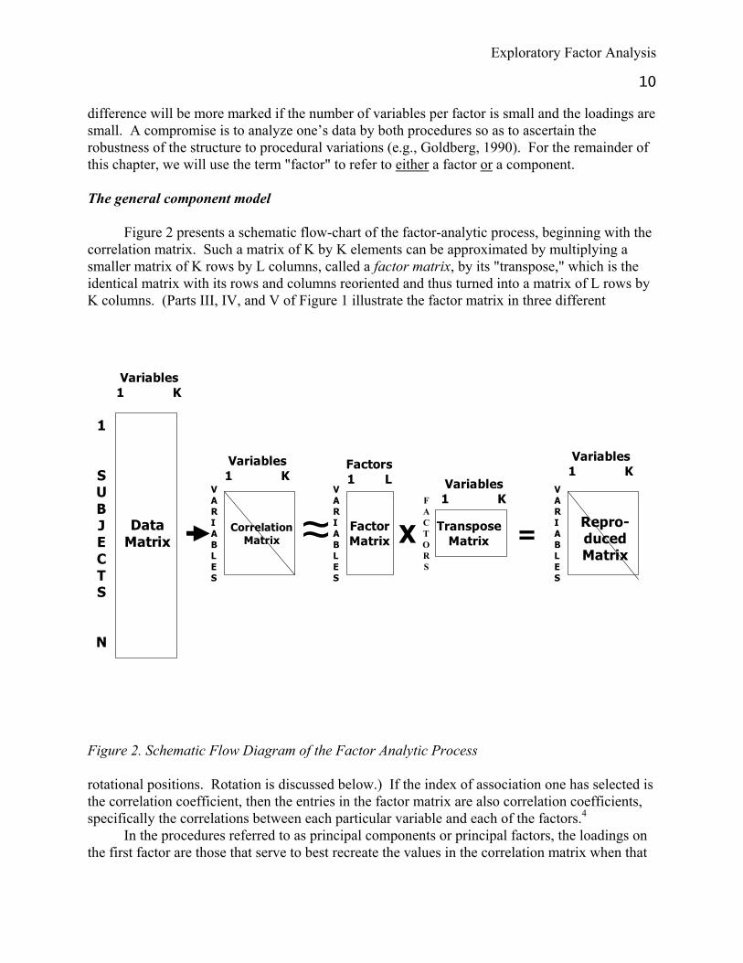
The general component model
Figure 2 presents a schematic flow-chart of the factor-analytic process, beginning with the
correlation matrix. Such a matrix of K by K elements can be approximated by multiplying a smaller matrix of K rows by L columns, called a factor matrix, by its "transpose," which is the identical matrix with its rows and columns reoriented and thus turned into a matrix of L rows by K columns. (Parts III, IV, and V of Figure 1 illustrate the factor matrix in three different
1
SUBJECTS
N
VARIABLES
VARIABLES
VARIABLES
=XDataMatrix
CorrelationMatrix
TransposeMatrix
Repro-ducedMatrix
FactorMatrix
Variables1 K
Variables1 K
Variables1 K
Variables1 KFactors
1 L
FACTORS
≈
Figure 2. Schematic Flow Diagram of the Factor Analytic Process rotational positions. Rotation is discussed below.) If the index of association one has selected is the correlation coefficient, then the entries in the factor matrix are also correlation coefficients, specifically the correlations between each particular variable and each of the factors.4
In the procedures referred to as principal components or principal factors, the loadings on the first factor are those that serve to best recreate the values in the correlation matrix when that

Exploratory Factor Analysis
11 factor matrix is multiplied by its transpose. Thus, the first principal factor provides a measure of whatever is most in common to the variables that have been included in the analysis. In the case of measures of aptitude or knowledge, the first principal factor has sometimes been considered to be an index of general ability or intelligence. In the case of personality variables, the first principal factor will typically be a blend of general evaluation (contrasting good versus bad attributes) and whatever particular content domain is most highly represented within the set of variables.
Moreover, each successive principal factor serves to best recreate the values in the correlation matrix after taking into account the factors extracted before it. Said another way, as each factor is extracted, the influence of that factor is partialed out of the correlations, leaving residual values that are independent of all factors that have been extracted. Thus, each factor is independent of all others; the intercorrelations among all pairs of factors are zero. (As noted below, this will no longer be true after an oblique rotation).
When factor analysis is used instead of component analysis, a researcher may encounter “improper” solutions (Thurstone, 1947), which are uninterpretable theoretically. For example, the estimate of the unique variance for one of the observed variables might be negative or zero. Some computer programs provide warnings and offer methods to “fix” the problem, such as constraining the estimates of the unique variances to be greater than zero (Joreskog, 1967). However, instead of correcting this problem with an ad hoc procedure, it would be better to diagnose the source of the problem. Van Driel (1978) described some of the causes of improper solutions. In simulation studies (Velicer & Fava, 1987, 1998), the probability of an improper solution increases when the number of variables per factor decreases, the sample size is small, or the factor leadings are small. In some cases, reducing the number of factors retained will solve the problem. In other cases, improving the selection of variables and/or the sample of subjects might be necessary.
Determining the optimal number of factors
After the factors have been extracted, one can multiply the factor matrix by its transpose to form a new K by K matrix, which is typically called a reproduced correlation matrix. As more factors are extracted, the differences between the values in the original and the reproduced matrices become smaller and smaller. If each value in the reproduced matrix is subtracted from its corresponding value in the original correlation matrix, the result is a K by K "residual" matrix, as shown in Figure 3. The more factors that are extracted, the better approximation of the original correlation matrix is provided by those factors, and thus the smaller are the values in the residual matrix. Consequently, if one's goal is to reproduce the original correlation matrix as precisely as possible, one will tend to extract many factors. On the other hand, the scientific principle of parsimony suggests that, other things being equal, fewer factors are better than many factors. One of the major decisions in factor analysis is the selection of the optimal number of factors, and this always involves a trade-off between extracting as few factors as possible versus recreating the original correlation matrix as completely as possible.

Exploratory Factor Analysis
12
VA R IA BLES1 K
VARIABLES
1
K
VA R IA BLES1 K
VARIABLES
1
K
VAR IAB LES1 K
VARIABLES
1
K
CorrelationM atrix R eproduced
M atrixR esidua l
M atrix
Figure 3. Schematic Flow Diagram of the Relation Between the Correlation Matrix, the Reproduced Matrix based on the first K Factors, and the Residual Matrix.
Over the years, many rules have been proposed to provide guidance on the number of factors to extract (e.g., Zwick & Velicer, 1986). Unfortunately, none of these rules will invariably guide the researcher to the scientifically most satisfactory decision. Perhaps even more unfortunately, one of the least satisfactory rules (the "eigenvalues greater than one" criterion, which will be explained later) is so easy to implement that it has been incorporated as the standard "default" option in some of the major statistical packages.
Figure 4 shows two indices that are typically derived from the factor matrix: "communalities" and "eigenvalues." A variable's communality is equal to the sum of the squared factor loadings in its row of the factor matrix. Thus, there are as many communality values as there are variables, and these values are normally provided as the final column of a factor matrix. In Part III of Figure 1, we include the communalities for all eight variables. The first variable (i.e., the first row) has a communality of (.65)2 + (.41)2 = .59. The communalities for the factor patterns presented in Part IV and Part V of Figure 1 are the same, except for rounding error.
The communality of a variable is the proportion of its variance that is associated with the total set of factors that have been extracted. That proportion can vary from zero to one. A variable with a communality of zero is completely independent of each of the factors. A variable with a communality of 1.00 can be perfectly predicted by the set of factors, when the factors are used as the predictors in a multiple regression equation and the variable itself is the criterion. In the "factor" model, these communalities are used to replace the original values of unity in the main diagonal of the correlation matrix.

Exploratory Factor Analysis
13
FactorMatrix
Factors1 L
COMMUNALITIES
1
K
VARIABLES
Eigenvalues
Figure 4. Schematic Flow Diagram of the Factor Pattern, the Eigenvalues, and Communalities.
The sums of the squared factor loadings down the columns of the principal component matrix are equal to the first of the "eigenvalues" (or "latent roots") of the correlation matrix from which the factors were derived. These values are normally provided in the bottom row in a factor matrix. In Figure 1, the eigenvalues are presented in Part II. In Part III of that figure, the sum of the squared loadings in the first two columns (2.79 and 1.55) is the same as the first two entries in the vector of eigenvalues. The eigenvalue associated with a factor is an index of its relative size: The eigenvalue associated with the first factor will always be at least as large, and normally much larger than, any of the others; and the eigenvalues of successive factors can never be larger, and will typically be smaller, than those that precede them. A plot of the size of the eigenvalues as a function of their factor number will appear as a rapidly descending concave curve that eventually becomes a nearly horizontal line. An example of such an eigenvalue plot (sometimes referred to as a "scree" plot, after Cattell, 1966) is provided in Figure 5. Included in that figure are the eigenvalues from a principal components analysis of 100 personality-descriptive adjectives, selected by Goldberg (1992) as markers of the Big-Five factor structure, in a sample of 636 self and peer ratings. This represents a better illustration than the eight-variable example in Figure 1 but the reader may want to graph the values in Part II of Figure 1 as a second example.

Exploratory Factor Analysis
14
0
2
4
6
8
10
12
0 10 20 30 40 50
Factor Number
Eige
nval
ue
Figure 5. Plot of the First 50 Eigenvalues from an Analysis of 100 Personality Adjectives.
Some of the rules for deciding on the optimal number of factors are based on the characteristics of such eigenvalue plots (e.g., Cattell, 1966). For example, if there is a very sharp break in the curve, with earlier eigenvalues all quite large relative to later ones that are all of similar size, then there is presumptive evidence that only the factors above the break should be retained. However, as indicated in Figure 5, although this highly selected set of variables provides an extremely clear five-factor structure, subjective interpretations of this eigenvalue plot could lead to decisions to extract 2, 5, 7, 8, 10, or 16 factors, depending on the preconceptions of the investigator. Indeed, it is quite rare for a plot of the eigenvalues to reveal unambiguous evidence of factor specification, and therefore alternative rules must be invoked.
One simple procedure is to examine the numerical value of each eigenvalue and to retain those above some arbitrary cutting point. Kaiser (1960) proposed that principal components with eigenvalues of 1.00 or above should be retained, and it is this quick-and-dirty heuristic that has been incorporated as the default option for factor extraction in some of the major statistical packages. In fact, however, the number of components with eigenvalues greater than one is highly related to the number of variables included in the analysis. Specifically, the number of eigenvalues greater than one will typically be in the range between one-quarter to one-third of the number of variables--no matter what the actual factor structure. (The number of factors with eigenvalues of 1.00 or above is 24 in the data displayed in Figure 5.) Simulation studies have consistently found this method to be very inaccurate (Zwick & Velicer, 1982; Zwick & Velicer, 1986; Velicer, Eaton, & Fava, 2000), and therefore the "eigenvalues greater than one" rule is not a reasonable procedure for deciding on the number of factors to extract. Another method based on the eigenvalues is Parallel Analysis, introduced by Horn (1965). This method was originally proposed as a means of improving the Kaiser rule by taking sampling error into account. In this method, a set of random data correlation matrices is generated,

Exploratory Factor Analysis
15 with the same number of variables and subjects as in the actual data matrix. The means of the eigenvalues across the set of random data matrices is calculated. The eigenvalues from the actual data are then compared to the mean eigenvalues of the random data. Components are retained as long as the eigenvalue from the actual data exceeds the eigenvalue from the random data. Figure 6 illustrates this procedure for the correlation matrix in Figure 1. The eigenvalues in Part II of Figure 1 are compared to the average eigenvalues from 8 random variables, with a sample size of 273. When the two eigenvalue sets are compared, this rule suggests the extraction of two factors. Simulation studies (Zwick & Velicer, 1986; Velicer, Eaton, & Fava, 2000) have found that parallel analysis is one of the most accurate methods.
0
0.5
1
1.5
2
2.5
3
1 2 3 4 5 6 7 8
Factor Numbe r
Eige
nval
ue
Figure 6. Illustration of the Parallel Analysis Procedure Applied to the Numerical Example in Figure 1. An alternative procedure is a statistical test associated with maximum-likelihood factor analysis. (There is a similar test for component analysis called the Bartlett test.) An asymptotic Chi-square test is calculated for each increase in the number of factors retained; the statistic becomes nonsignificant when the eigenvalues associated with the remaining factors do not differ significantly with each other, at which point it is assumed that the correct number of factors has been discovered. This test has not performed well in evaluative studies (Velicer, Eaton, & Fava, 2000), in part because it is so highly sensitive to the sample size. When the number of subjects becomes even moderately large or the observed variables depart even moderately from the assumption of multivariate normalacy, it will result in retaining too many factors. The Minimum Average Partial-correlation (MAP: Velicer, 1976) method for finding
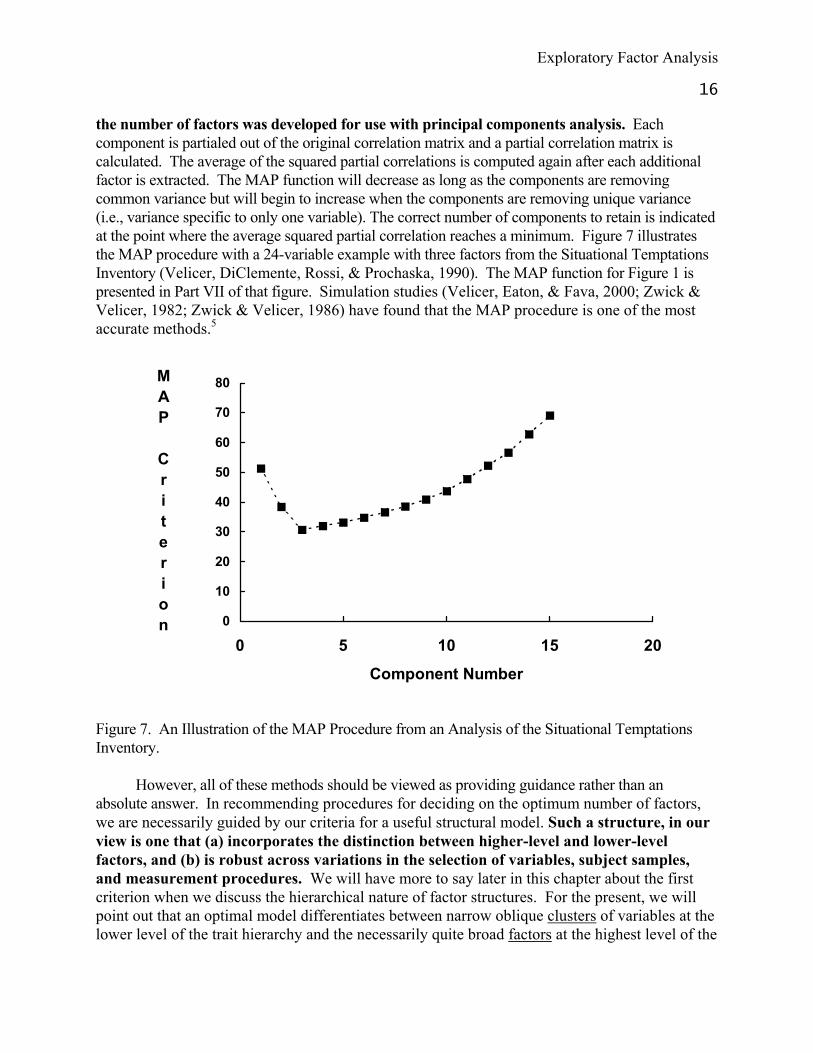
Exploratory Factor Analysis
16 the number of factors was developed for use with principal components analysis. Each component is partialed out of the original correlation matrix and a partial correlation matrix is calculated. The average of the squared partial correlations is computed again after each additional factor is extracted. The MAP function will decrease as long as the components are removing common variance but will begin to increase when the components are removing unique variance (i.e., variance specific to only one variable). The correct number of components to retain is indicated at the point where the average squared partial correlation reaches a minimum. Figure 7 illustrates the MAP procedure with a 24-variable example with three factors from the Situational Temptations Inventory (Velicer, DiClemente, Rossi, & Prochaska, 1990). The MAP function for Figure 1 is presented in Part VII of that figure. Simulation studies (Velicer, Eaton, & Fava, 2000; Zwick & Velicer, 1982; Zwick & Velicer, 1986) have found that the MAP procedure is one of the most accurate methods.5
0
10
20
30
40
50
60
70
80
0 5 10 15 20
Component Number
MAP Criterion
Figure 7. An Illustration of the MAP Procedure from an Analysis of the Situational Temptations Inventory.
However, all of these methods should be viewed as providing guidance rather than an absolute answer. In recommending procedures for deciding on the optimum number of factors, we are necessarily guided by our criteria for a useful structural model. Such a structure, in our view is one that (a) incorporates the distinction between higher-level and lower-level factors, and (b) is robust across variations in the selection of variables, subject samples, and measurement procedures. We will have more to say later in this chapter about the first criterion when we discuss the hierarchical nature of factor structures. For the present, we will point out that an optimal model differentiates between narrow oblique clusters of variables at the lower level of the trait hierarchy and the necessarily quite broad factors at the highest level of the

Exploratory Factor Analysis
17 structure.
In studies of personality traits, there appear to be at least five broad higher-level factors (Digman, 1990; Goldberg, 1990; John, 1990; McCrae & John, 1992; Wiggins & Pincus, 1992), whereas at levels that are lower in the hierarchy the number of such factors varies enormously, reflecting the theoretical predilections of different investigators. In the explicitly hierarchical models of Cattell (1957) and of McCrae and Costa (1985, 1987), Cattell argued for 16 lower-level factors in analyses of the items in his Sixteen Personality Factors Questionnaire, whereas Costa and McCrae (1992) provide scales to measure 30 lower-level factors in the revised version of their NEO Personality Inventory. Both Cattell and Costa and McCrae have claimed substantial evidence of factor robustness across subject samples (although not of course across differing selections of variables), and their disagreements could simply reflect differences in the vertical locations of their factors (clusters) within the overall hierarchical structure.
In any case, there seems to be widespread agreement that an optimal factor structure is one that is comparable over independent studies, and we advocate the incorporation of this principle into any procedure for deciding on the number of factors to extract (see Everett, 1983; Nunnally, 1978). What this means is that no single analysis is powerful enough to provide evidence of the viability of a factor structure; what is needed are two or more (preferably many more) analyses of at least somewhat different variables in different subject samples.
Rotating the factors
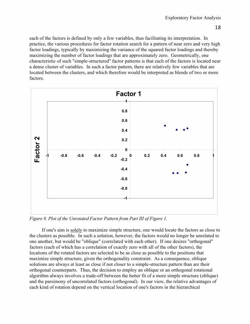
The factor matrix displayed in Figure 2 includes K rows (one row for each variable) and L columns (one column for each of the L factors that have been extracted). Multiplying the factor matrix by its transpose produces the K by K reproduced matrix. However, there are an infinite number of K by L matrices which when multiplied by their transposes will produce that identical reproduced matrix. Each of these "rotations" of the original factor matrix has the same set of communality values (the sums of the squared factor loadings within each row). Matrices included in this family of factor rotations differ from one another in the relative sizes of their factors, as indexed by the sums of squared factor loadings down the columns. Given any particular set of data, the unrotated principal factors have the steepest possible descending pattern of factor variances (i.e., eigenvalues). At the other extreme, it is possible to obtain a factor matrix in which each factor is of approximately the same size. Figure 8 illustrates the original unrotated factor pattern presented in Part III of Figure 1. The factor loadings in Part III correspond to the projection of the eight points (the items) onto the two axes (the factors). The sum of the squared loadings in each column of the factor pattern correspond to the first two eigenvalues (2.79 and 1.55). The first unrotated factor is located in the position that maximizes its variance across all eight variables, and the second unrotated factor is orthogonal to the first. As is usually the case, however, these two unrotated factors do not pass through any of the dense clusters of variables.
Indeed, the unrotated factors do not normally have much scientific utility, except in a few quite limited contexts.6 Instead, the criterion usually invoked for selecting the optimal rotation is that of "simple structure," which informally can be defined as a pattern of factor loadings that contains a few high values in each column, with the rest mostly around zero. Such a factor pattern is "simple" in the sense that most variables have high loadings on only one factor and
Exploratory Factor Analysis
18 each of the factors is defined by only a few variables, thus facilitating its interpretation. In practice, the various procedures for factor rotation search for a pattern of near zero and very high factor loadings, typically by maximizing the variance of the squared factor loadings and thereby maximizing the number of factor loadings that are approximately zero. Geometrically, one characteristic of such "simple-structured" factor patterns is that each of the factors is located near a dense cluster of variables. In such a factor pattern, there are relatively few variables that are located between the clusters, and which therefore would be interpreted as blends of two or more factors.
-1
-0.8
-0.6
-0.4
-0.2
0
0.2
0.4
0.6
0.8
1
-1 -0.8 -0.6 -0.4 -0.2 0 0.2 0.4 0.6 0.8 1
Factor 1
Fact
or 2
Figure 8. Plot of the Unrotated Factor Pattern from Part III of Figure 1.
If one's aim is solely to maximize simple structure, one would locate the factors as close to the clusters as possible. In such a solution, however, the factors would no longer be unrelated to one another, but would be "oblique" (correlated with each other). If one desires "orthogonal" factors (each of which has a correlation of exactly zero with all of the other factors), the locations of the rotated factors are selected to be as close as possible to the positions that maximize simple structure, given the orthogonality constraint. As a consequence, oblique solutions are always at least as close if not closer to a simple-structure pattern than are their orthogonal counterparts. Thus, the decision to employ an oblique or an orthogonal rotational algorithm always involves a trade-off between the better fit of a more simple structure (oblique) and the parsimony of uncorrelated factors (orthogonal). In our view, the relative advantages of each kind of rotation depend on the vertical location of one's factors in the hierarchical

Exploratory Factor Analysis
19 representation: If one seeks lower-level factors within a single domain, we recommend the use of an oblique rotation. On the other hand, if one seeks broad higher-level factors, we recommend the use of an orthogonal rotation.
By far the most commonly used procedure for orthogonal factor rotation is the "varimax" algorithm of Kaiser (1958), which is available in all of the statistical packages. The numeric values for the orthogonal (varimax) rotated pattern are presented in Part IV of Figure 1. Figure 9 illustrates the orthogonal rotation for this data. Note that the two axes are now more closely aligned with the two item clusters.
The problem of providing an optimal algorithm for oblique rotations is more complex than that for the orthogonal case, and there is less uniformity in the oblique rotational options provided by the major statistical packages. Indeed, the particular algorithm that we prefer, one called "promax" (Hendrickson & White, 1964), is not included in all of the popular factor programs. We will use the readily available oblimin rotation to illustrate the method. The numeric values for the oblique (oblimin) rotated pattern are listed in Part V of Figure 1. Figure 10 illustrates the oblique rotation for these data. The two axes are now almost perfectly aligned with the two item clusters but they are no longer at right angles to each other.
-1
-0.8
-0.6
-0.4
-0.2
0
0.2
0.4
0.6
0.8
1
-1 -0.8 -0.6 -0.4 -0.2 0 0.2 0.4 0.6 0.8 1
Factor 1
Fact
or 2
Figure 9. Plot of the Orthogonal (Varimax) Rotated Factor Pattern from Part IV of Figure 1.
After an orthogonal rotation, the resulting factor matrix of K rows by L columns can be interpreted in the same way as the original unrotated matrix: Its entries are the correlations

Exploratory Factor Analysis
20 between each of the variables and each of the factors. The relative size of a particular unrotated or rotated factor can be indexed by the sum of its squared factor loadings down the column, but for the rotated factors these sums can no longer be referred to as eigenvalues, which have distinct mathematical properties based on the original correlation matrix. When each of the sums of squared factor loadings down a column of a factor matrix is divided by the number of variables in the analysis, the resulting ratio indicates the proportion of the total variance from all variables that is provided by that factor.
-1
-0.8
-0.6
-0.4
-0.2
0
0.2
0.4
0.6
0.8
1
-1 -0.8 -0.6 -0.4 -0.2 0 0.2 0.4 0.6 0.8 1
Factor 1
Fact
or 2
Figure 10. Plot of the Oblique (Oblimin) Rotated Factor Pattern from Part V of Figure 1.
In the case of an oblique rotation, there are three meaningful sets of factor-loading coefficients that can be interpreted: (a) The factor pattern, or the regression coefficients linking the factors to the variables; (b) the factor structure, or the correlations between the variables and each of the factors; and (c) the reference vectors, or the semi-partial (also called part) correlations between the variables and each of the factors, after the contributions of the other factors have been partialed out. In addition, it is necessary to obtain the correlations among the factors. With orthogonal factors, all three sets of factor-loading coefficients are the same, and

Exploratory Factor Analysis
21 the correlations among all pairs of factors are zero. Calculating factor scores
One important use of factor analysis is to discover the relations between factors in one domain and variables from other domains (which in turn might be other sets of rotated factors). One way to obtain such relations is to score each subject in the sample on each of the factors, and then to correlate these "factor scores" with the other variables included in the study. The major statistical computing packages provide such factor scores upon request. In component analyses, the component scores are calculated directly, whereas in factor analysis they must be estimated. The best methods of factor-score estimation (McDonald & Burr, 1967) include the Thurstone (1935) regression estimate, the Bartlett (1937) residual minimization estimate, and the Anderson and Rubin (1956) constrained residual minimization method. All three of these methods are based on the data from a single sample, and when that sample is small in size, these values may not be particularly robust across different subject samples (Dawes, 1979). More robust should be less sample-dependent coefficients such as a simple weighting of the variables by 1.00, 0.0, and –1.00 corresponding to the size and direction of their factor loadings. This type of procedure is typically referred to as providing “scale” scores. However, the choice of method does not represent a critical decision in factor analysis. Simulation studies have found that the correlation between component scores, factor score estimates, and the simpler scale scores calculated on the same data typically exceed .96 (Fava & Velicer, 1992).
Finally, a number of factor theorists eschew the use of factor scores altogether, preferring to use alternative "extension" methods of relating factors to other variables (McDonald, 1978). When one requests factor scores from one of the major statistical packages, orthogonal components lead to orthogonal factor scores (unfortunately, this is not necessarily the case with orthogonal factors). However, even with orthogonal components, if one develops scales by selecting items with high factor loadings on each of those components, it is likely that these scales will be related to each other. In general, the reason for the sizeable correlations among scales derived from orthogonal factors is that (a) there are few factor-univocal items, most items having secondary factor loadings of substantial size, and (b) if one selects items solely on the basis of their highest factor loading, it is extremely unlikely that the secondary loadings will completely balance out. To decrease the intercorrelations among such scales, one needs to take secondary loadings into account (Saucier, 2002; Saucier & Goldberg, 2002), for which purpose one may want to use a procedure such as the AB5C model of Hofstee, de Raad, and Goldberg (1992), which will be described later.
Vertical and Horizontal Aspects of Factor Structures in Personality
Like most concepts, personality-trait constructs include both vertical and horizontal
features. The vertical aspect refers to the hierarchical relations among traits (e.g., ‘Reliability’ is a more abstract and general concept than ‘Punctuality’), whereas the horizontal aspect refers to the degree of similarity among traits at the same hierarchical level (e.g., ‘Sociability’ involves aspects of both Warmth and Activity Level). Scientists who emphasize the vertical aspect of

Exploratory Factor Analysis
22 trait structure could employ multivariate techniques such as hierarchical cluster analysis, or they could employ oblique rotations in factor analysis, and then factor the correlations among the primary dimensions, thus constructing a hierarchical structure. Scientists who emphasize the horizontal aspect of trait structure could employ discrete cluster solutions or orthogonal factor rotations.
Historically, however, there has been no simple relation between the emphases of investigators and their methodological preferences. For example, both Eysenck (1970) and Cattell (1947) have developed explicitly hierarchical representations, Eysenck's leading to three highest-level factors, Cattell's to eight or nine. However, whereas Cattell has always advocated and used oblique factor procedures, Eysenck has typically preferred orthogonal methods. In the case of the more recent five-factor model, some of its proponents construe the model in an expressly hierarchical fashion (e.g., Costa, McCrae, & Dye, 1991; McCrae & Costa, 1992), whereas others emphasize its horizontal aspects (e.g., Peabody & Goldberg, 1989; Hofstee, de Raad, & Goldberg, 1992).
Vertical approaches to trait structure
The defining feature of hierarchical models of personality traits is that they emphasize the vertical relations among variables (e.g., from the most specific to the most abstract), to the exclusion of the relations among variables at the same level. One of the most famous hierarchical models of individual differences is the classic Vernon-Burt hierarchical model of abilities (e.g., Vernon, 1950); specific test items are combined to form ability tests, which are the basis of specific factors, which in turn are the basis of the minor group factors, which in turn lead to the major group factors, which at their apex form the most general factor, "g" for general intelligence.
Another classic example of a hierarchical structure is Eysenck's (1970) model of Extraversion; specific responses in particular situations (e.g., telling a joke, buying a new car) are considered as subordinate categories to habitual responses (e.g., entertaining strangers, making rapid decisions), which in turn make up such traits as Sociability and Impulsiveness, which finally form the superordinate attribute of Extraversion. Horizontal approaches to trait structure
The defining feature of horizontal models is that the relations among the variables are specified by the variables' locations in multidimensional factor space. When that space is limited to only two dimensions, and the locations of the variables are projected to some uniform distance from the origin, the resulting structures are referred to as "circumplex" representations. The most famous example of such models is the Interpersonal Circle (e.g., Wiggins, 1979, 1980; Kiesler, 1983), which is based on Factors I (Surgency) and II (Agreeableness) in the Big-Five model. Other examples of circumplex models involve more than a single plane, including the three-dimensional structures that incorporate Big-Five Factors I, II, and III (Stern, 1970; Peabody & Goldberg, 1989), and Factors I, II, and IV (Saucier, 1992). A more comprehensive circumplex representation has been proposed by Hofstee, de Raad, and Goldberg (1992). Dubbed the "AB5C" model, for Abridged Big Five-dimensional Circumplex, this representation includes the ten bivariate planes formed from all pairs of the Big-Five factors.
Exploratory Factor Analysis
23 Comparing vertical and horizontal perspectives
All structural representations based on factor-analytic methodology can be viewed from either vertical or horizontal perspectives. Factor analysis can be used to construct hierarchical models explicitly with oblique rotational procedures and implicitly even with orthogonal solutions, since any factor can be viewed as being located at a level above that of the variables being factored; that is, even orthogonal factors separate the common variance (the factors) from the total (common plus unique) variance of the measures. One could therefore emphasize the vertical aspect by grouping the variables by the factor with which they are most highly associated, thereby disregarding information about factorial blends. Alternatively, one could concentrate on the horizontal features of the representation, as in the AB5C model. What are the advantages associated with each perspective?
McCrae and Costa (1992) have argued that hierarchical structures are to be preferred to the extent to which the variances of the lower-level traits are trait-specific, as compared to the extent that they are related to the five broad factors. These investigators demonstrated that, after partialing out the five-factor common variance from both self and other ratings on the facet scales from the revised NEO Personality Inventory (Costa & McCrae, 1992), the residual variance in these scales was still substantial enough to elicit strong correlations among self ratings, spouse ratings, and peer ratings of the same lower-level trait. From this finding, they argued in favor of hierarchical representations, in which relatively small amounts of common variance produce the higher-level factors, with ample amounts of unique variance still available for predictive purposes.
This argument has powerful implications for the role of trait measures when used in multiple regression analyses in applied contexts, such as personnel selection and classification. In thinking about items, scales, and factors, it is important to distinguish between the common and the unique variance of the variables at each hierarchical level. Any time that two or more variables are amalgamated, the variance that is unique to each of them is lost, and only their common variance is available at the higher amalgamated level. That is, most of the variance of individual items is lost when items are averaged into scale scores, and most of the variance of personality scales is lost when they are combined in factors. Indeed, most of the variance of personality scales is specific variance, not the common variance that is associated with the higher-level factor domains. And, therefore, for purposes of optimal prediction in applied contexts one should descend the hierarchical structure as far as sample size (and thus statistical power) permits. Other things being equal, the optimal number of predictors to be included in a regression analysis varies directly with the size of the subject sample; for large samples, one can include more variables than can be included in small samples, where one can more easily capitalize on the chance characteristics of the sample and thus lose predictive robustness when one applies the regression weights in new samples.
Summary and Conclusions
Over more years than we'd like to admit, each of the two authors of this chapter has independently carried out hundreds of factor analyses. Although our intellectual roots differ substantially, we tend to agree on most of the controversial issues in the field. For example, with

Exploratory Factor Analysis
24 regard to two of the most vexing decisions--the use of factor analysis versus component analysis and the use of orthogonal versus oblique rotations--our experience suggests that in the realms of personality and psychopathology these choices are not very important, at least with well-structured data sets. In general, the more highly structured are one's data, the less it matters which factor-analytic decisions one makes. Indeed, the best way to assure oneself about a factor structure is to analyze the data in different ways, and thereby test the robustness of one's solution across alternative procedures.
On the other hand, two decisions are of considerable importance--the initial selection of variables and the number of factors to extract. The selection of variables should be guided by theory and/or the findings from past research. Because we believe that an optimal factor structure is one that is comparable over independent studies, we advocate the incorporation of this principle into any procedure for deciding on the number of factors to extract. What this means is that no single analysis is powerful enough to provide definitive evidence of the viability of a factor structure; what is needed are multiple analyses of at least somewhat different variables in different subject samples.
Moreover, the comparison of solutions from different subject samples will almost always be more useful when the complete hierarchical structures are available. To do this requires the analysis at differing hierarchical levels, which in practice means the repeated analyses of the same data set extracting different numbers of factors. One can begin with the first unrotated component, then examine the two-factor varimax-rotated solution, then the three-factor representation, stopping only when a new factor does not include at least two variables with their highest loadings on it. If one rotates the factors at each level, and computes orthogonal factor scores on these rotated factors, then one can intercorrelate the set of all factor scores, and thus discover the relations between the factors at differing levels. For examples of such hierarchical representations, see Goldberg (1999), Goldberg and Somer (2000), Goldberg and Strycker (2002), and Saucier (1997, 2000, 2003). A hierarchical perspective has powerful implications for the role of trait measures when used in multiple regression analyses in applied contexts, such as personnel selection and classification. Because one loses some unique variance as one amalgamates measures, the optimal level of prediction is a function of statistical power, and thus of sample size. Other things being equal, the optimal number of predictors to be included in a regression analysis varies directly with the size of the subject sample; for large samples, one can include more variables than can be included in small samples, which more easily capitalize on chance characteristics and thus lose predictive robustness when one applies the regression weights in new samples.
However, a horizontal perspective is necessary for basic research on trait structure, because trait variables are not clustered tightly in five-dimensional space; rather, most variables share some features with one set of variables while they share other features with another set. Thus, even after rotation of the factors to a criterion of simple structure such as varimax, most variables have substantial secondary loadings, and thus must be viewed as blends of two or more factors. Because hierarchical models de-emphasize these horizontal aspects of trait relations, they provide no information about the nature of such factorial blends. For purposes of basic research on the structure of traits, therefore, models that emphasize horizontal relations such as the AB5C model will typically be more informative.
In concluding this chapter, we acknowledge the fact that many investigators are now

Exploratory Factor Analysis
25 turning away from exploratory factor analysis altogether in favor of confirmatory models and procedures; indeed, a spate of new textbooks deal exclusively with confirmatory models, whereas the most recent of the major textbooks that focus primarily on exploratory techniques was published over two decades ago (Gorsuch, 1983). For readers who may be curious about our continued use of exploratory factor analysis in the face of the emerging consensus against it, we will now try to provide some justification for our beliefs.
First of all, it is important to realize that most applications of confirmatory models involve, by our standards, extremely small sets of variables; a typical confirmatory analysis includes only a dozen or two dozen variables, and applications of these models to variable sets of the sizes we work with (e.g., Goldberg, 1990, 1992) are still computationally prohibitive. Second, an increase in the number of factors can result in a reduction in the size of some fit indices (Marsh, Hau, Balla, & Grayson, 1998). Applied researchers often substitute arbitrary sums of subsets of the observed variables called “item parcels” to address this problem. Third, as much as we support theory-driven research, we recognize that most work in personality and psychopathology often falls on a continuum between the testing of a well-established theory and the development of a new theoretical model. Very few studies represent pure examples of theory testing.
Moreover, we view exploratory and confirmatory procedures as complementary rather than as competing. From this viewpoint, it is more appropriate to talk about a program of research rather than a single study and use both methods at different times during the planned set of studies. In addition, we have a concern about the problem of a confirmatory bias. Greenwald, Pratkanis, Leippe, and Baumgardner (1986) distinguish between theory-oriented and result-centered research. These two types of investigations roughly correspond to confirmatory and exploratory approaches. In their criticism of theory-oriented research, Greenwald et al. warn about the tendency to persevere by modifying procedures and not reporting results that are inconsistent with the theory. There are numerous examples in the literature where an initial failure to confirm was followed by a reliance on modification indices such as the use of correlated error terms.
In contrast, repeated independent discoveries of the same factor structure derived from exploratory techniques provide stronger evidence for that structure than would be provided by the same number of confirmatory analyses. In other words, if results replicate and the analysis does not involve a target, the results can be viewed as more independently tested than if the data are fitted to a specified model. Indeed, when a confirmatory analysis is used to reject a model (which will virtually always occur if the sample is large enough), the investigator's subsequent tinkering with the model can be viewed as a return to exploratory analysis procedures.
Although we have not been impressed with the substantive knowledge of personality structure that has yet accrued from findings based on confirmatory techniques, we applaud their development, and we encourage their use. We suspect that when theories of personality structure become specified more precisely, perhaps on the basis of findings from exploratory analyses, we will see the advantages of confirmatory factor models over exploratory ones. In the interim, we believe that there is a substantial role for both types of methodologies.
References
Anderson, T. W., & Rubin, H. (1956). Statistical inference in factor analysis. In J. Neyman

Exploratory Factor Analysis
26 (Ed.), Proceedings of the third Berkeley symposium on mathematical statistics and probability (pp. 111-150). Berkeley, CA: University of California.
Bartlett, M. S. (1937). The statistical conception of mental factors. British Journal of Psychology, 28, 97-104.
Cattell, R. B. (1947). Confirmation and clarification of primary personality factors. Psychometrika, 12, 197-220.
Cattell, R. B. (1957). Personality and motivation structure and measurement. Yonkers-on-Hudson, NY: World Book.
Cattell, R. B. (1966). The scree test for the number of factors. Multivariate Behavioral Research, 1, 245-276.
Costa, P. T., Jr., & McCrae, R. R. (1992). Revised NEO Personality Inventory (NEO-PI-R) and NEO Five-Factor Inventory (NEO-FFI) professional manual. Odessa, FL: Psychological Assessment Resources.
Costa, P. T., Jr., McCrae, R. R., & Dye, D. A. (1991). Facet scales for Agreeableness and Conscientiousness: A revision of the NEO Personality Inventory. Personality and Individual Differences, 12, 887-898.
Dawes, R. M. (1979). The robust beauty of improper linear models in decision making. American Psychologist, 34, 571-582.
Digman, J. M. (1990). Personality structure: Emergence of the five-factor model. In M. R. Rosenzweig & L. W. Porter (Eds.), Annual Review of Psychology: Vol. 41 (pp. 417-440). Palo Alto, CA: Annual Reviews.
Everett, J. E. (1983). Factor comparability as a means of determining the number of factors and their rotation. Multivariate Behavioral Research, 18, 197-218.
Eysenck, H. J. (1970). The structure of human personality: Third edition. London: Methuen.
Fava, J. L., & Velicer, W. F. (1992). An empirical comparison of factor, image, component, and scale scores. Multivariate Behavioral Research, 27, 301-322.
Goldberg, L. R. (1981). Language and individual differences: The search for universals in personality lexicons. In L. Wheeler (Ed.), Review of Personality and Social Psychology: Vol. 2 (pp. 141-165). Beverly Hills, CA: Sage.
Goldberg, L. R. (1990). An alternative "Description of personality": The Big-Five factor structure. Journal of Personality and Social Psychology, 59, 1216-1229.
Goldberg, L. R. (1992). The development of markers for the Big-Five factor structure. Psychological Assessment, 4, 26-42.
Goldberg, L. R. (1999). The Curious Experiences Survey, a revised version of the Dissociative Experiences Scale: Factor structure, reliability, and relations to demographic and personality variables. Psychological Assessment, 11, 134-145.
Goldberg, L. R., & Digman, J. M. (1994). Revealing structure in the data: Principles of exploratory factor analysis. In S. Strack and M. Lorr (Eds.), Differentiating normal and abnormal personality (pp. 216-242). New York: Springer.
Goldberg, L. R., & Somer, O. (2000). The hierarchical structure of common Turkish person-descriptive adjectives. European Journal of Personality, 14, 497-531.
Goldberg, L. R., & Strycker, L. A. (2002). Personality traits and eating habits: The assessment of food preferences in a large community sample. Personality and Individual Differences, 32, 49-65.

Exploratory Factor Analysis
27
Gorsuch, R. L. (1983). Factor analysis (2nd Edition). Hillsdale, NJ: Erlbaum. Graham, J. W., Cumsille, P. E., & Elek-Fisk, E. (2003). Methods for handling missing
data. In J. A. Schinka & W. F. Velicer (Eds.), Research methods in psychology: Handbook of psychology (Vol. 2: pp. 87-114). New York: Wiley.
Greenwald, A. G., Pratkanis, A. R., Leippe, M. R., & Baumgardner, M. H. (1986). Under what conditions does theory obstruct research progress? Psychological Review, 93, 216-229.
Guadagnoli, E., & Velicer, W. F. (1988). Relation of sample size to the stability of component patterns. Psychological Bulletin, 103, 265-275.
Harman, H. H. (1976). Modern factor analysis (3rd Edition). Chicago, IL: University of Chicago.
Hendrickson, A. E., & White, P. O. (1964). Promax: A quick method of rotation to oblique simple structure. British Journal of Statistical Psychology, 17, 65-70.
Hofstee, W. K. B., de Raad, B., & Goldberg, L. R. (1992). Integration of the Big Five and circumplex taxonomies of traits. Journal of Personality and Social Psychology, 63, 146-163.
Horn, J. L. (1965). A rationale and test for the number of factors in factor analysis. Psychometrika, 30, 179-185.
Hotelling, H. (1933). Analysis of a complex of statistical variables into principal components. Journal of Educational Psychology, 24, 417-441, 498-520.
John, O. P. (1990). The "Big-Five" factor taxonomy: Dimensions of personality in the natural language and in questionnaires. In L. A. Pervin (Ed.), Handbook of personality theory and research (pp. 66-100). New York: Guilford.
Joreskog, K. G. (1967). Some contributions to maximum likelihood factor analysis. Psychometrika, 32, 443-482.
Kaiser, H. F. (1958). The varimax criterion for analytic rotation in factor analysis. Psychometrika, 23, 187-200.
Kaiser, H. F. (1960). The application of electronic computers to factor analysis. Educational and Psychological Measurement, 20, 141-151.
Kiesler, D. J. (1983). The 1982 interpersonal circle: A taxonomy for complementarity in human transactions. Psychological Review, 90, 185-214.
Little, R. J. A., & Rubin, D. B. (1987). Statistical analysis with missing data. New York: Wiley.
MacCallum, R. C., Widaman, K. F., Zhang, S., & Hong, S. (1999). Sample size in factor analysis. Psychological Methods, 4, 84-99.
Marsh, H. W., Hau, K.-T., Balla, J. R., & Grayson, D. (1998). Is more ever too much? The number of indicators per factor in confirmatory factor analysis. Multivariate Behavioral Research, 33, 181-220.
McCrae, R. R., & Costa, P. T., Jr. (1985). Updating Norman's "adequate taxonomy": Intelligence and personality dimensions in natural language and in questionnaires. Journal of Personality and Social Psychology, 49, 710-721.
McCrae, R. R., & Costa, P. T., Jr. (1987). Validation of the five-factor model of personality across instruments and observers. Journal of Personality and Social Psychology, 52, 81-90.
McCrae, R. R., & Costa, P. T., Jr. (1992). Discriminant validity of NEO-PIR facet scales. Educational and Psychological Measurement, 52, 229-237.
McCrae, R. R., & John, O. P. (1992). An introduction to the five-factor model and its

Exploratory Factor Analysis
28 applications. Journal of Personality, 60, 175-215.
McDonald, R. P. (1978). Some checking procedures for extension analysis. Multivariate Behavioral Research, 13, 319-325.
McDonald, R. P. (1985). Factor analysis and related methods. Hillsdale, NJ: Erlbaum. McDonald, R. P., & Burr, E. J. (1967). A comparison of four methods of constructing
factor scores. Psychometrika, 32, 381-401. Mulaik, S. A. (1972). The foundations of factor analysis. New York: McGraw-Hill. Nunnally, J. (1978). Psychometric theory (2nd Edition). New York: McGraw-Hill. O’Connor, B. P. (2002). The search for dimensional structure differences between
normality and abnormality: A statistical review of published data on personality and psychopathology. Journal of Personality and Social Psychology, 83, 962-982.
Peabody, D., & Goldberg, L. R. (1989). Some determinants of factor structures from personality-trait descriptors. Journal of Personality and Social Psychology, 57, 552-567.
Pearson, K. (1901). On lines and planes of closest fit to systems of points in space. Philosophical Magazine, Series B, 2, 559-572.
Prochaska, J. O., Velicer, W. F., Rossi, J. S., Goldstein, M. G., Marcus, B. H., Rakowski, W., Fiore, C., Harlow, L. L., Redding, C. A., Rosenbloom, D., & Rossi, S. R. (1994). Stages of change and decisional balance for twelve problem behaviors. Health Psychology, 13, 39-46.
Saucier, G. (1992). Benchmarks: Integrating affective and interpersonal circles with the Big-Five personality factors. Journal of Personality and Social Psychology, 62, 1025-1035.
Saucier, G. (1997). Effects of variable selection on the factor structure of person descriptors. Journal of Personality and Social Psychology, 73, 1296-1312.
Saucier, G. (2000). Isms and the structure of social attitudes. Journal of Personality and Social Psychology, 78, 366-385.
Saucier, G. (2002). Orthogonal markers for orthogonal factors: The case of the Big Five. Journal of Research in Personality, 36, 1-31.
Saucier, G. (2003). Factor structure of English-language personality type-nouns. Journal of Personality and Social Psychology, 85, 695-708.
Saucier, G., & Goldberg, L. R. (2002). Assessing the Big Five: Applications of 10 psychometric criteria to the development of marker scales. In B. de Raad & M. Perugini (Eds.), Big Five assessment (pp. 29-58). Goettingen, Germany: Hogrefe & Huber.
Saucier, G., & Goldberg, L. R. (2003). The structure of personality attributes. In M. R. Barrick & A. M. Ryan (Eds.), Personality and work: Reconsidering the role of personality in organizations (pp. 1-29). San Francisco, CA: Jossey-Bass.
Schafer, J. L. (1997). Analysis of Incomplete Multivariate Data. New York: Wiley. Schafer, J. L., & Graham, J. W. (2002). Missing data: Our view of the state of the art.
Psychological Methods, 7, 147-177. Serlin, R. C., & Kaiser, H. F. (1976). A computer program for item selection based on
maximum internal consistency. Educational and Psychological Measurement, 36, 757-759. Spearman, C. (1904). General intelligence, objectively determined and measured.
American Journal of Psychology, 15, 201-293. Stern, G. G. (1970). People in context: Measuring person-environment congruence in
education and industry. New York: Wiley. ten Berge, J. M. F. (1999). A legitimate case of component analysis of ipsative measures,
and partialing the mean as an alternative to ipsatization. Multivariate Behavioral Research, 34,

Exploratory Factor Analysis
29 89-102.
Thomas, C., Turkheimer, E., & Oltmanns, T. F. (2003). Factorial structure of pathological personality as evaluated by peers. Journal of Abnormal Psychology, 112, 81-91.
Thurstone, L. L. (1931). Multiple factor analysis. Psychological Review, 38, 406-427. Thurstone, L. L. (1935). The vectors of the mind. Chicago, IL: University of Chicago. Thurstone, L. L. (1947). Multiple factor analysis. Chicago, IL: University of Chicago. Van Driel, O. P. (1978). On various causes of improper solutions in maximum likelihood
factor analysis. Psychometrika, 43, 225-243. Velicer, W. F. (1976). Determining the number of components from the matrix of partial
correlations. Psychometrika, 4l, 32l-327. Velicer, W. F., DiClemente, C. C., Prochaska, J. O., & Brandenberg, N. (1985). A
decisional balance measure for assessing and predicting smoking status. Journal of Personality and Social Psychology, 48, 1279-1289.
Velicer, W. F., DiClemente, C., Rossi, J. S., & Prochaska, J. O. (1990). Relapse situations and self-efficacy: An integrative model. Addictive Behaviors, 15, 271-283.
Velicer, W. F., Eaton, C. A., & Fava, J. L. (2000). Construct explication through factor or component analysis: A review and evaluation of alternative procedures for determining the number of factors or components. In R. D. Goffin & E. Helmes (Eds.), Problems and solutions in human assessment: Honoring Douglas Jackson at seventy (pp. 41-71). Boston, MA: Kluwer.
Velicer, W. F., & Fava, J. L. (1987). An evaluation of the effects of variable sampling on component, image, and factor analysis. Multivariate Behavioral Research, 22, 193-210.
Velicer, W. F., & Fava, J. L. (1998). The effects of variable and subject sampling on factor pattern recovery. Psychological Methods, 3, 231-251.
Velicer, W. F., & Jackson, D. N. (1990). Component analysis versus common factor analysis: Some issues in selecting an appropriate procedure. Multivariate Behavioral Research, 25, 1-28.
Vernon, P. E. (1950). The structure of human abilities. London: Methuen. Ward, R. M., Velicer, W. F., Rossi, J. S., Fava, J. L., & Prochaska, J. O. (2004). Factorial
invariance and internal consistency for the Decisional Balance Inventory—Short Form. Addictive Behaviors, 29, 953-958.
Wiggins, J. S. (1979). A psychological taxonomy of trait-descriptive terms: The interpersonal domain. Journal of Personality and Social Psychology, 37, 395-412.
Wiggins, J. S. (1980). Circumplex models of interpersonal behavior. In L. Wheeler (Ed.), Review of personality and social psychology (Vol. 1, pp. 265-294). Beverly Hills, CA: Sage.
Wiggins, J. S., & Pincus, A. L. (1992). Personality: Structure and assessment. In M. R. Rosenzweig & L. W. Porter (Eds.), Annual Review of Psychology (Vol. 43, pp. 473-504). Palo Alto, CA: Annual Reviews.
Zegers, F. E., & ten Berge, J. M. F. (1985). A family of association coefficients for metric scales. Psychometrika, 50, 17-24.
Zwick, W. R., & Velicer, W. F. (1982). Factors influencing four rules for determining the number of components to retain. Multivariate Behavioral Research, 17, 253-269.
Zwick, W. R., & Velicer, W. F. (1986). Comparison of five rules for determining the number of components to retain. Psychological Bulletin, 99, 432-442.

Exploratory Factor Analysis
30
Endnotes
1. Items: 1 = Smoking cigarettes relieves tension; 2 = I am embarrassed to have to smoke; 3 = Smoking helps me concentrate and do better work; 4 = My cigarette smoking bothers other people; 5 = I am more relaxed and therefore more pleasant when smoking; 6 = People think that I am foolish for ignoring the warnings about cigarette smoking; 7 = Smoking cigarettes is pleasurable; 8 = Smoking cigarettes is hazardous to my health. 2. Response Format: 1 = NOT IMPORTANT; 2 = SLIGHTLY IMPORTANT; 3 = MODERATELY IMPORTANT; 4 = VERY IMPORTANT; 5 = EXTREMELY IMPORTANT. 3. Even for multi-step rating scales, when subjects respond to hundreds of items on the same occasion, there are typically large individual differences in the means and the variances of the subjects' response distributions across the items. Some of these differences may stem from such response biases as Extremeness Response Style (a tendency to use the polar categories of the rating scale versus the middle ones) and Acquiescence Response Set (a tendency to agree rather than to disagree with items, regardless of their content). To attenuate individual differences in such response biases, investigators may elect to standard (Z) score each subject's responses separately across the total set of items. Standard scoring can be useful for items rated on continuous scales, for dichotomous response formats, and even for items administered in a checklist. However, standard scoring may also serve to remove important individual differences when the item pool includes more items keyed in one direction than the other on any of the underlying dimensions. Under those conditions, one might consider more complex procedures, such as those developed by ten Berge (1999). 4. The explanations in this section only apply to the original matrix of principal factors, which are "orthogonal," and not to the subsequent "rotated" matrices, which may be "oblique." 4. Although many popular computer programs do not include the Parallel Analysis or MAPS procedures, readers can obtain SPSS and SAS programs to compute them at the following web-site: http://flash.lakeheadu.ca/~boconno2/boconnor.html 6. The first unrotated principal component has some properties that make it useful when all of the variables under analysis have been selected as measures of the exact same construct. Given that it provides an index of whatever is most in common to the variables, it can sometimes be used as a surrogate for the underlying "latent" construct, and its loadings then can be viewed as reflecting the correlations of each variable with that construct. In our experience, however, the most useful application of the first unrotated component is with tasks in which judges rate a common set of stimuli on some attribute. In such a situation, one can correlate the judges' ratings across the set of stimuli to index the extent to which pairs of raters agree with one another. The first unrotated principal component of this matrix of interjudge agreement correlations reflects the group consensus, and the factor loadings of each judge on this first component indicates that judge's correlation with the consensus. The factor scores for each stimulus on this component are the optimal scale values for that stimulus, when judges are weighted by their contribution to the group consensus. The Coefficient Alpha reliability of these factor scores is equal to N / (N - 1) x (E - 1) / E, where E is the eigenvalue of the component and

Exploratory Factor Analysis
31 N is the number of judges (Serlin & Kaiser, 1976).