principles and applications of fluorescence spectroscopy
TRANSCRIPT

Principles and Applications ofFluorescence Spectroscopy
Jihad René AlbaniLaboratoire de Biophysique MoléculaireUniversité des Sciences et Technologies de LilleFrance

This page intentionally left blank

Principles and Applications ofFluorescence Spectroscopy
Jihad René AlbaniLaboratoire de Biophysique MoléculaireUniversité des Sciences et Technologies de LilleFrance

©2007 by Jihad Rene Albani
Blackwell Science, a Blackwell Publishing companyEditorial offices:Blackwell Science Ltd, 9600 Garsington Road, Oxford OX4 2DQ, UK
Tel: +44 (0) 1865 776868Blackwell Publishing Professional, 2121 State Avenue, Ames, Iowa 50014-8300, USA
Tel: +1 515 292 0140Blackwell Science Asia Pty Ltd, 550 Swanston Street, Carlton, Victoria 3053, Australia
Tel: +61 (0)3 8359 1011
The right of the Author to be identified as the Author of this Work has been asserted in accordance with theCopyright, Designs and Patents Act 1988.
All rights reserved. No part of this publication may be reproduced, stored in a retrieval system, or transmitted, inany form or by any means, electronic, mechanical, photocopying, recording or otherwise, except as permitted bythe UK Copyright, Designs and Patents Act 1988, without the prior permission of the publisher.
Designations used by companies to distinguish their products are often claimed as trademarks. All brand namesand product names used in this book are trade names, service marks, trademarks or registered trademarks oftheir respective owners. The Publisher is not associated with any product or vendor mentioned in this book.
This publication is designed to provide accurate and authoritative information in regard to the subject mattercovered. It is sold on the understanding that the Publisher is not engaged in rendering professional services. Ifprofessional advice or other expert assistance is required, the services of a competent professional should besought.
First published 2007
ISBN 978-1-4051-3891-8
Library of Congress Cataloging-in-Publication DataAlbani, Jihad Rene , 1956-
Principles and applications of fluorescence spectroscopy / Jihad Rene Albani.p. ; cm.
Includes bibliographical references and index.ISBN-13: 978-1-4051-3891-8 (pbk. : alk. paper)ISBN-10: 1-4051-3891-2 (pbk. : alk. paper) 1. Fluorescence spectroscopy. I. Title.[DNLM: 1. Spectrometry, Fluorescence. 2. Biochemistry. QD 96.F56 A326p 2007]QP519.9.F56A43 2007543′.56–dc22
2006100265
A catalogue record for this title is available from the British Library
Set in 10/12 Minionby Newgen Imaging Systems (P) Ltd, Chennai, IndiaPrinted and bound in Malaysiaby KHL Printing Co Sdn Bhd
The publisher’s policy is to use permanent paper from mills that operate a sustainable forestry policy, and whichhas been manufactured from pulp processed using acid-free and elementary chlorine-free practices.Furthermore, the publisher ensures that the text paper and cover board used have met acceptable environmentalaccreditation standards.
For further information on Blackwell Publishing, visit our website:www.blackwellpublishing.com
Contents
1 Absorption Spectroscopy Theory 11.1 Introduction 11.2 Characteristics of an Absorption Spectrum 21.3 Beer–Lambert–Bouguer Law 41.4 Effect of the Environment on Absorption Spectra 6References 11
2 Determination of the Calcofluor White Molar Extinction Coefficient Value inthe Absence and Presence of α1-Acid Glycoprotein 132.1 Introduction 132.2 Biological Material Used 13
2.2.1 Calcofluor White 132.2.2 α1-Acid glycoprotein 13
2.3 Experiments 162.3.1 Absorption spectrum of Calcofluor free in PBS buffer 162.3.2 Determination of ε. value of Calcofluor White free in
PBS buffer 162.3.3 Determination of Calcofluor White ε. value in the presence of
α1-acid glycoprotein 162.4 Solution 17References 19
3 Determination of Kinetic Parameters of Lactate Dehydrogenase 213.1 Objective of the Experiment 213.2 Absorption Spectrum of NADH 213.3 Absorption Spectrum of LDH 223.4 Enzymatic Activity of LDH 223.5 Kinetic Parameters 223.6 Data and Results 22
3.6.1 Determination of enzyme activity 233.6.2 Determination of kinetic parameters 23
3.7 Introduction to Kinetics and the Michaelis–Menten Equation 26

iv Contents
3.7.1 Definitions 263.7.2 Reaction rates 26
References 32
4 Hydrolysis of p-Nitrophenyl-β-D-Galactoside with β-Galactosidasefrom E. coli 344.1 Introduction 344.2 Solutions to be Prepared 354.3 First-day Experiments 35
4.3.1 Absorption spectrum of PNP 354.3.2 Absorption of PNP as a function of pH 364.3.3 Internal calibration of PNP 374.3.4 Determination of β-galactosidase optimal pH 394.3.5 Determination of β-galactosidase optimal temperature 40
4.4 Second-day Experiments 404.4.1 Kinetics of p-nitrophenyl-β-D-galactoside hydrolysis with
β-galactosidase 404.4.2 Determination of the β-galactosidase concentration in the test
tube 424.5 Third-day Experiments 44
4.5.1 Determination of Km and Vmax of β-galactosidase 444.5.2 Inhibiton of hydrolysis kinetics of p-nitrophenyl-β-D-galactoside 45
4.6 Fourth-day Experiments 474.6.1 Effect of guanidine chloride concentration on β-galactosidase
activity 474.6.2 OD variation with guanidine chloride 484.6.3 Mathematical derivation of Keq 484.6.4 Definition of the standard Gibbs free energy, �G◦′ 514.6.5 Relation between �G◦′ and �G ′ 514.6.6 Relation between �G◦′ and Keq 524.6.7 Effect of guanidine chloride onhydrolysis kinetics of
p-nitrophenyl-β-D-galactoside 56References 57
5 Starch Hydrolysis by Amylase 595.1 Objectives 595.2 Introduction 595.3 Materials 615.4 Procedures and Experiments 61
5.4.1 Preparation of a 20 g l −1starch solution 615.4.2 Calibration curve for starch concentration 615.4.3 Calibration curve for sugar concentration 635.4.4 Effect of pH 645.4.5 Temperature effect 665.4.6 Effect of heat treatment at 90◦C 695.4.7 Kinetics of starch hydrolysis 70

Contents v
5.4.8 Effect of inhibitor (CuCl2) on the amylase activity 735.4.9 Effect of amylase concentration 735.4.10 Complement experiments that can be performed 775.4.11 Notes 77
References 78
6 Determination of the pK of a Dye 796.1 Definition of pK 796.2 Spectrophotometric Determination of pK 796.3 Determination of the pK of 4-Methyl-2-Nitrophenol 81
6.3.1 Experimental procedure 816.3.2 Solution 83
References 87
7 Fluorescence Spectroscopy Principles 887.1 Jablonski Diagram or Diagram of Electronic Transitions 887.2 Fluorescence Spectral Properties 91
7.2.1 General features 917.2.2 Stokes shift 937.2.3 Relationship between the emission spectrum and
excitation wavelength 947.2.4 Inner filter effect 957.2.5 Fluorescence excitation spectrum 957.2.6 Mirror–image rule 957.2.7 Fluorescence lifetime 967.2.8 Fluorescence quantum yield 1017.2.9 Fluorescence and light diffusion 102
7.3 Fluorophore Structures and Properties 1027.3.1 Aromatic amino acids 1047.3.2 Cofactors 1087.3.3 Extrinsinc fluorophores 108
7.4 Polarity and Viscosity Effect on Quantum Yield and Emission MaximumPosition 111
References 113
8 Effect of the Structure and the Environment of a Fluorophore onIts Absorption and Fluorescence Spectra 115Experiments 115Questions 117Answers 119Reference 123
9 Fluorophore Characterization and Importance in Biology 1249.1 Experiment 1. Quantitative Determination of Tryptophan in Proteins in
6 M Guanidine 1249.1.1 Introduction 124

vi Contents
9.1.2 Principle 1249.1.3 Experiment 1259.1.4 Results obtained with cytochrome b2 core 126
9.2 Experiment 2. Effect of the Inner Filter Effect on Fluorescence Data 1279.2.1 Objective of the experiment 1279.2.2 Experiment 1279.2.3 Results 128
9.3 Experiment 3. Theoretical Spectral Resolution of Two EmittingFluorophores Within a Mixture 1309.3.1 Objective of the experiment 1309.3.2 Results 132
9.4 Experiment 4. Determination of Melting Temperature of Triglycerides inSkimmed Milk Using Vitamin A Fluorescence 1349.4.1 Introduction 1349.4.2 Experiment to conduct 1369.4.3 Results 136
References 138
10 Fluorescence Quenching 13910.1 Introduction 13910.2 Collisional Quenching: the Stern–Volmer Relation 14010.3 Different Types of Dynamic Quenching 14510.4 Static Quenching 147
10.4.1 Theory 14710.5 Thermal Intensity Quenching 154References 159
11 Fluorescence Polarization 16011.1 Definition 16011.2 Fluorescence Depolarization 162
11.2.1 Principles and applications 16211.3 Fluorescence Anisotropy Decay Time 16511.4 Depolarization and Energy Transfer 166References 167
12 Interaction Between Ethidium Bromide and DNA 16812.1 Objective of the Experiment 16812.2 DNA Extraction from Calf Thymus or Herring Sperm 168
12.2.1 Destruction of cellular structure 16812.2.2 DNA extraction 16812.2.3 DNA purification 16912.2.4 Absorption spectrum of DNA 169
12.3 Ethidium Bromide Titration with Herring DNA 16912.4 Results Obtained with Herring DNA 170
12.4.1 Absorption and emission spectra 17012.4.2 Analysis and interpretation of the results 173

Contents vii
12.5 Polarization Measurements 17712.6 Results Obtained with Calf Thymus DNA 17912.7 Temperature Effect on Fluorescence of the Ethidium Bromide–DNA
Complex 180References 182
13 Lens culinaris Agglutinin: Dynamics and Binding Studies 18413.1 Experiment 1. Studies on the Accessibility of I− to a Fluorophore:
Quenching of Fluorescein Fluorescence with KI 18413.1.1 Objective of the experiment 18413.1.2 Experiment 18413.1.3 Results 185
13.2 Experiment 2. Measurement of Rotational Correlation Time ofFluorescein Bound to LCA with Polarization Studies 18713.2.1 Objective of the work 18713.2.2 Polarization studies as a function of temperature 18713.2.3 Polarization studies as a function of sucrose at 20◦C 18713.2.4 Results 189
13.3 Experiment 3. Role of α-L-fucose in the Stability ofLectin–Glycoproteins Complexes 19013.3.1 Introduction 19013.3.2 Binding studies 19113.3.3 Results 192
References 196
14 Förster Energy Transfer 19714.1 Principles and Applications 19714.2 Energy-transfer Parameters 20214.3 Bioluminescence Resonance Energy Transfer 204References 208
15 Binding of TNS on Bovine Serum Albumin at pH 3 and pH 7 21015.1 Objectives 21015.2 Experiments 210
15.2.1 Fluorescence emission spectra of TNS–BSA at pH 3 and 7 21015.2.2 Titration of BSA with TNS at pH 3 and 7 21015.2.3 Measurement of energy transfer efficiency from Trp residues
to TNS 21115.2.4 Interaction between free Trp in solution and TNS 211
15.3 Results 211
16 Comet Test for Environmental Genotoxicity Evaluation: A FluorescenceMicroscopy Application 22016.1 Principle of the Comet Test 22016.2 DNA Structure 22016.3 DNA Reparation 221

viii Contents
16.4 Polycyclic Aromatic Hydrocarbons 22216.5 Reactive Oxygen Species 22316.6 Causes of DNA Damage and Biological Consequences 22416.7 Types of DNA Lesions 225
16.7.1 Induction of abasic sites, AP, apurinic, or apyrimidinic 22516.7.2 Base modification 22516.7.3 DNA adducts 22516.7.4 Simple and double-stranded breaks 225
16.8 Principle of Fluorescence Microscopy 22516.9 Comet Test 227
16.9.1 Experimental protocol 22716.9.2 Nature of damage revealed with the Comet test 22716.9.3 Advantages and limits of the method 22716.9.4 Result expression 231
References 231
17 Questions and Exercises 23217.1 Questions 232
17.1.1 Questions with shorts answers 23217.1.2 Find the error 23217.1.3 Explain 23317.1.4 Exercises 234
17.2 Solutions 24117.2.1 Questions with short answers 24117.2.2 Find the error 24317.2.3 Explain 24317.2.4 Exercises solutions 244
Index 253
Color plate appears between pages 168 and 169

Chapter 1Absorption Spectroscopy Theory
1.1 Introduction
With reference to absorption spectroscopy, we deal here with photon absorption by electronsdistributed within specific orbitals in a population of molecules. Upon absorption, oneelectron reaches an upper vacant orbital of higher energy. Thus, light absorption wouldinduce the molecule excitation. Transition from ground to excited state is accompaniedby a redistribution of an electronic cloud within the molecular orbitals. This conditionis implicit for transitions to occur. According to the Franck–Condon principle, electronictransitions are so fast that they occur without any change in nuclei position, that is, nucleihave no time to move during electronic transition. For this reason, electronic transitionsare always drawn as vertical lines.
The energy of a pair of atoms as a function of the distance separating them is given bythe Morse curve (Figure 1.1). Re is the equilibrium bond distance. At this distance, themolecule is in its most stable position, and so its energy is called the molecular equilibriumenergy, which is expressed as E0 or Ee. Stretching or compressing the bond induces anenergy increase. On the left-hand side of Re, the two atoms become increasingly closer,inducing repulsion forces. Thus, an energy increase will be observed as a consequence ofthese repulsion forces. On the right-hand side of Re, the distance between the two atomsincreases, and there will be attraction forces so that an equilibrium distance can be reached.Thus, an energy increase will be observed as result of the attraction forces. In principle, aharmonic oscillation should be obtained, but this is not the case. In fact, beyond a certaindistance between the two atoms, the attraction forces will exert no more influence, andattraction energy will reach a plateau. Therefore, the Morse curve is anharmonic.
The energy within a molecule is the sum of several distinct energies:
E (total) = E (translation) + E (rotation) + E (vibration)
+ E (electronic) + E (electronic orientation of spin)
+ E (nuclear orientation of spin) (1.1)
The rotational energy concerns molecular rotation around its gravity center, vibrationalenergy is the result of periodic displacement of atoms of the molecule away from theequilibrium position, and electronic energy is generated by electron movement withinthe molecular bonds. Rotational levels have lower energy than vibrational ones and thusare lower in energy. Upon photon absorption, electronic, rotational, and vibrational levels

2 Principles and Applications of Fluorescence Spectroscopy
43
1
0
2
1
−1 0 1 2 3 4 5
v = 0
De
Vmax
V/h
cDe
Do
a(R −Re)
Figure 1.1 Morse curve characterizing the energy of the molecule as a function of the distance R thatseparates the atoms of a diatomic molecule such as hydrogen. At a distance equal to Re, which correspondsto point 0, the molecule is in its most stable position, and so its energy is called the molecular equilibriumenergy and expressed as Ee. Stretching or compressing the bond yields an increase in energy. The numberof bound levels is finite. D0 is the dissociation energy and De the dissociation minimum energy. Thehorizontal lines correspond to the vibrational levels.
participate in this phenomenon; therefore, energy absorbed by a molecule is equal to the sumof energies absorbed by electronic, vibrational, and rotational energy levels. In fluorescenceor phosphorescence, all three levels release energy. Finally, it is important to mention thatmolecules that absorb photons are called chromophores.
1.2 Characteristics of an Absorption Spectrum
An absorption spectrum is the result of electronic, vibrational, and rotational transitions.The spectrum maximum (the peak) corresponds to the electronic transition line, andthe rest of the spectrum is formed by a series of lines that correspond to rotational andvibrational transitions. Therefore, absorption spectra are sensitive to temperature. Raisingthe temperature increases the rotational and vibrational states of the molecules and inducesthe broadening of the recorded spectrum.
The profile of the absorption spectrum depends extensively on the relative positionof the Er value, which depends on the different vibrational states. The intensity of theabsorption spectrum depends, among others, on the population of molecules reachingthe excited state. The more important is this population, the higher the intensity of thecorresponding absorption spectrum will be. Therefore, recording absorption spectrum ofthe same molecule at different temperatures should yield, in principle, an altered or modifiedabsorption spectrum.

Absorption Spectroscopy Theory 3
A spectrum is characterized by its peak position (the maximum), and the full width athalf maximum, which is equal to the difference
δν = ν2 − ν1 (1.2)
ν1 and ν2 correspond to the frequencies that are equal to half the maximal intensity.If the molecules studied do not display any motions, the spectral distribution will display
a Lorenzian-type profile. In this case, the probability of the electronic transition Ei → Ef isidentical for all molecules that belong to the Ei level.
Thermal motion induces different displacement speeds for the molecules and thusdifferent transition probabilities. These change from one molecule to another and from onepopulation of molecules to another. In this case, the spectral distribution will be Gaussian.The full width at half maximum of a Gaussian spectrum is greater than that of a Lorenzianspectrum.
The spectrophotometer should have a thermostat in situ during the experiment and bepositioned away from the sun; otherwise, the temperature of the spectrophotometer’s innerelectronics would increase, possibly introducing important errors in the optical density(OD) measurements. In addition, exposing the spectrophotometer to sunlight can inducecontinuous fluctuations in the OD, thus making any serious measurements impossible.
Absorption spectrum is the plot of light intensity as a function of wavelength. Figure 1.2shows the absorption spectra of tryptophan, tyrosine, and phenylalanine in water. A strongband at 210–220 nm and a weaker band at 260–280 nm can be seen.
40,000
20,000
10,000
5,000
2,000
1,000
500
300
100
50
20
102000 2200 2400 2600
Wavelengrth (Å)
2800 3000 3200
ε, M
olar
abs
orpr
ivity
PHE
TYR
TRY
Figure 1.2 Absorption spectra of tryptophan, tyrosine and phenylalanine in water. Source:Wetlaufer, D.B.(1962). Advances in Protein Chemistry, 17, 303–390.

4 Principles and Applications of Fluorescence Spectroscopy
Soret0.45
0.36
0.27
0.19
OD
0.09
0.00400 500
Wavelength (nm)600
IVIII
II I
Figure 1.3 Absorption spectrum of protoporphyrin IX dissolved in DMSO.
A molecule can have one, two, or several absorption peaks or bands (Figure 1.3). Theband located at the highest wavelength and therefore having the weakest energy is called thefirst absorption band. In the visible range between 500 and 650 nm, porphyrins display fourabsorption bands. The intensity ratios between these bands are a function of the natureof lateral chains “carried” by the pyrrolic ring. These bands are the results of electronictransitions of nitrogen atoms of the pyrrolic ring. Metalloporphyrins show two degeneratedbands α and β that result, respectively, from the association of bands I and III and bands IIand IV.
1.3 Beer–Lambert–Bouguer Law
An absorption spectrum is characterized by two parameters, the maximum position (λmax)
and the molar extinction coefficient (ε) calculated in general at λmax. The relation betweenε, sample concentration (c), and thickness (l) of the absorbing medium is characterized bythe Beer–Lambert–Bouguer law. Since the solution studied is placed in a cuvette, and themonochromatic light beam passes through the cuvette, the thickness of the sample is calledthe optical path length or simply the path length.
While passing through the sample, light is partly absorbed, and the spectrophotometerwill record theoretically nonabsorbed or transmitted light. Plotting the transmittance, which

Absorption Spectroscopy Theory 5
1.0
0.8
0.6
0.4
0.2
Tran
smitt
ance
, I/I
o
00 1.0 2.0
Pathlength, d (cm)
3.0 4.0
1
2
10
Figure 1.4 Transmittance variation with optical pathlength for three sample concentrations.
is the ratio of transmitted light IT over incident light I0:
T = IT/I0 (1.3)
as a function of optical path length and sample concentration yields an exponential decrease(Figure 1.4).
Therefore, T is proportional to exponential (−cl):
T ∝ e−cl (1.4)
Equation (1.4) can also be written as
ln T = ln(IT/I0) ∝ −cl (1.5)
A proportionality constant k can be introduced, yielding
ln T = ln(IT/I0) = −kcl (1.6)
− ln T = ln(I0/IT) = kcl (1.7)
Transforming Equation (1.7) to a decimal logarithm, we obtain
− log T = log(I0/IT) = kcl
2.3= εcl = OD = A (1.8)
Equation (1.8) is the Beer–Lambert–Bouguer law. At each wavelength, we have a precise OD.Since the absorption or OD is equal to a logarithm, it does not have any unity. Concentrationc is expressed in molar (M) or mol l−1, the optical path length in centimetres (cm), andthus ε in M−1 cm−1.
ε characterizes the absorption of 1 mol l−1 of solution. This is called the extinctioncoefficient because incident light going through the solution is partly absorbed. Thus,the light intensity is “quenched” and is attenuated or inhibited while passing through thesolution.

6 Principles and Applications of Fluorescence Spectroscopy
If the concentration is expressed in mg ml−1 or in g l−1, the unity of ε will be in mg−1 ml ·cm−1 or g−1 l cm−1. Conversion to M−1 cm−1 is possible by multiplying the value of ε
expressed in g−1 l cm−1 by the chromophore molar mass.In general, ε is determined at the highest absorption wavelength(s), since molecules
absorb most at these wavelengths. However, it is possible to calculate an ε at every wavelengthof the absorption spectrum.
In proteins, three amino acids, tryptophan, tyrosine, and phenylalanine, are responsiblefor UV absorption. ε in proteins is determined at the maximum (278 nm) (Figure 1.2),and thus protein concentrations are calculated by measuring absorbance at this wavelength.Cystine and the ionized sulfhydryl groups of cysteine absorb also in this region but theirabsorption is weaker than the three aromatic amino acids. Ionization of the sulfhydryl groupinduces an increase in the absorption and the appearance of a new peak around 240 nm.The imidazole group of histidine absorbs in the 185–220 nm region. Finally, importantabsorption of the peptide bonds occurs at 190 nm.
When a protein possesses a prosthetic group such as heme, its concentration is usuallydetermined at the absorption wavelengths of the heme. The most important absorptionband of heme is called the Soret band and is localized around 408–425 nm. The peakposition of the Soret band depends on the heme structure, and in cytochromes, this willdepend on whether cytochrome is oxidized or reduced.
Chromophores free in solution and bound to macromolecules do not display identical εvalues and absorption peaks. For example, free hemin absorbs at 390 nm. However, in thecytochrome b2 core extracted from the yeast Hansenula anomala, the absorption maximumof heme is located at 412 nm with a molar extinction coefficient equal to 120 mM−1 cm−1
(Albani 1985). In the same way, protoporphyrin IX dissolved in 0.1 N NaOH absorbs at510 nm, whereas when it is bound to apohemoglobin, it absorbs in the Soret band at around400 nm.
1.4 Effect of the Environment on Absorption Spectra
The environment here can be the temperature, solvent, chromophore interaction withanother molecule, etc.
In general, the interaction between the solvent and the chromophore occurs viaelectrostatic interactions and hydrogen bonds. In the presence of a highly polar solvent,the dipole–dipole interaction requires a high amount of energy, and thus the position ofthe absorption peak will be located at low wavelengths. On the contrary, when the dipole–dipole interaction is weak such as when the chromophore is dissolved in a solvent of lowpolarity, the energy required for absorption is weak, i.e., the position of the absorption bandis located at high wavelengths. A blue shift in the absorption band is called the hypsochromicshift, and a red shift is called the bathochromic shift.
When the chromophore binds to proteins, the binding site is generally more hydrophobicthan the solution. Therefore, one should expect to observe a shift in the absorptionband to the highest wavelength compared to the peak observed when the chromophoreis free in solution. The following example of absorption spectroscopy, specificallyrelated to a prosthetic group in proteins, is the vanadate-containing enzyme vanadiumchloroperoxidase (VCPO) from the fungus Curvularia inaequalis. This enzyme primarily
Absorption Spectroscopy Theory 7
Arg-360His-496Lys-353
Ser-402
Gly-403
His-404
Arg-490
Asp-292
N COV
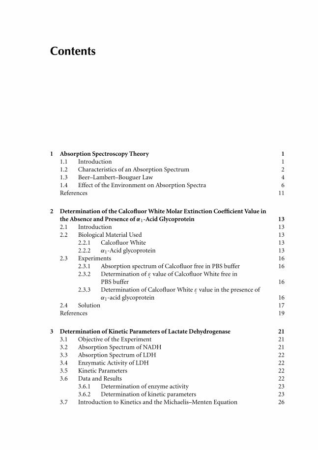
Figure 1.5 Vanadate binding in VCPO from C. inaequalis, determined at pH 8.3 (PDB: 1IDQ). Source:Plass,W. (1999).Angewandte Chemie, 38, 909–912. Reprinted with permission fromWiley-Intersciences.
catalyzes halide oxidation to hypohalous acids at the expense of hydrogen peroxideEquation (1.9). C. inaequalis is a plant parasite, and VCPO is considered to be involvedin the breakdown of the lignin structures of plant leaves (Wever et al. 2006). In vitro, VCPOalso catalyzes sulfoxidation (Andersson et al. 1997; Ten Brink et al. 1999).
H2O2 + X− + H+ → HOX + H2O X = Cl, Br, or I (1.9)
The VCPO active site, displayed in Figure 1.5, shows the binding environment of vanadate(HVO2−
4 ), as determined by X-ray crystallography (Messerschmidt et al. 1997). The cofactoris directly bound to a histidine residue (His496), and the position of the nonproteinvanadate oxygens is stabilized by a hydrogen-bonding network. The resulting structure is atrigonal bipyramid with one apical Nε2 nitrogen of His496, and the other apical position isconsidered to be a hydroxide, based on the V−−O bond length (1.96 Å). The negative chargeon the three equatorial oxygens is stabilized by three positively charged residues, Arg490,Arg360, and Lys353. A minimal catalytic scheme of VCPO is shown in Figure 1.6, also basedon the X-ray structure of VCPO crystals soaked in H2O2, the first substrate of the enzyme(Messerschmidt et al. 1997; Hasan et al. 2006).
The UV-VIS spectrum of 100 μM VCPO at pH 8.3 is displayed in Figure 1.7a, whichshows the spectra of apo-, holo-, and holo-enzyme after the addition of the first substrateH2O2 (peroxo-intermediate) (Renirie et al. 2000a). If a halide is added to the peroxo-intermediate, the holo-spectrum is reformed, in line with the scheme shown in Figure 1.6.

8 Principles and Applications of Fluorescence Spectroscopy
OH
O O−
H
N
N
HN
HN
H2O2′ 2H+H2O
2H2O
−O
−OX−
HOX
O
ON
N
Vv
VvVvO
+
Lys353
His496
His496
Lys353
H+
Figure 1.6 Minimal catalytic scheme of VCPO based on crystal structures of the native enzyme and theperoxo-intermediate (Messerschmidt et al. 1997). Lys353 is considered to be crucial in assisting heterolyticcleavage of the side-on bound peroxide. EPR and V-EXAFS data suggest that the enzyme remains in theVV oxidation state throughout the cycle. Source: Hasan, Z., Renirie, R., Kerkman, R., Ruijssenaars, H.J.,Hartog, A.F. and Wever, R. (2006). Journal of Biological Chemistry, 281, 9738–9744. Reprinted withpermission from Renirie, R., Hemrika, W., Piersma, S.R. and Wever, R. (2000). Biochemistry, 39,1133–1141. Copyright © 2000 American Chemical Society.
1.0 0.5
0.4
0.3
0.2
0.1
Δ A
bsor
banc
e (3
16 n
m)
0.0
0.8
0.6
0.4
0.2
Abs
orba
nce
0.0
300 350 400
Wavelength (nm)
Wavelength (nm)
450
Holo minus apo
300holo
peroxo
apo
400
500 550 0 50 100 150
[Vanadate] (�M)
200 250 300
(a) (b)
Figure 1.7 (a) UV-VIS absorption spectra of 100 μM vanadium chloroperoxidase at pH 8.3. The lowersolid line shows the apo-enzyme, the upper solid line the holo-enzyme after addition of 100 μM vanadate.The dotted line is the peroxo-form of the enzyme after addition of 100 μMH2O2. (b) Titration of apo-CPOwith vanadate; changes in the optical absorbance at 316 nm (•). Absorbance of free vanadate under thesame buffer conditions (©). Reprinted with permission from Renirie, R., Hemrika, W., Piersma, S.R. andWever, R. (2000). Biochemistry, 39, 1133–1141. Copyright © 2000 American Chemical Society.

Absorption Spectroscopy Theory 9
The inset shows the difference spectrum of holo minus apo-VCPO, with a maximum at 315nm, with �ε = 2.8 mM−1. The remaining absorption of the peroxo-intermediate at 315nm is �ε = 0.7 mM−1 cm−1. Titration of apoprotein with vanadate, shown in Figure 1.7b,shows stochiometric binding and a very high affinity of the protein for the cofactor (Renirieet al. 2000a).
Figure 1.8 showsVCPO titration with H2O2, confirming the high affinity for this substrateas observed in steady-state experiments by Hemrika et al. (1999). Figure 1.9 shows that
0.2
0.1
Δ A
bsor
banc
e (3
16 n
m)
0.0
0 50
[H2O2] (�M)
100 150
Figure 1.8 Titration of 100μMVCPOwithH2O2 at pH8.3. Source: Renirie, R., Hemrika,W., Piersma, S.R.and Wever, R. (2000). Biochemistry, 39, 1133–1141. Reprinted with permission from The AmericanChemical Society © 2000.
0.2
Δ A
bsor
banc
e
0.0
−0.2
−0.4
−0.6
−0.8300 400
Wavelength (nm)
500 600
ab
Figure 1.9 Spectrum a: Difference spectrum for 300 μM peroxo-VCPO minus holo-VCPO. Spectrum b:Difference spectrum for 300 μM pervanadate minus vanadate. Source: Renirie, R., Hemrika, W.,Piersma, S.R. and Wever, R. (2000). Biochemistry, 39, 1133–1141. Reprinted with permission from TheAmerican Chemical Society © 2000.

10 Principles and Applications of Fluorescence Spectroscopy
addition of H2O2 also results in a small positive band at 384 nm (a), which is red-shifted ascompared to free peroxovanadate (b).
In native VCPO, the position and intensity of cofactor-induced absorption are sensitive topH change; at pH 5, the band is blue-shifted (λmax∼308 nm), and the intensity is decreasedto ε = 2.0 mM−1 cm−1. The exact correlation between the above-mentioned spectralfeatures and the known X-ray data are complex, but a further UV-VIS analysis of severalmutants of this enzyme showed the importance of several structural elements. A His496Alamutant showed no optical spectrum (Hemrika et al. 1999), whereas crystal structure ofthis mutant showed the presence of tetrahedral vanadate in the active site (Macedo-Ribeiroet al. 1999), indicating that the V−−N bond is crucial for the observed spectrum. The effectof other mutations can be seen in Table 1.1.
Figure 1.10 shows the mutation effect of the catalytically important His404 on thespectrum and illustrates how the spectrum can be used to observe changes in the vanadate
Table 1.1 Extinction coefficients of holo minus apo VCPO and mutants and dissociation constants forvanadate determined from absorption spectroscopy at pH 8.3
Enzyme �ε (holo−apo) λ Kd (vanadate) Reference
VCPO 2.8 mM−1 cm−1 316 nm <20 μM Renirie et al. (2000a)H496A No spectrum observed — — Renirie et al. (2000a)H404A 2.1 mM−1 cm−1 316 nm 112 ± 3 μM Renirie et al. (2000b)R360A 1.5 mM−1 cm−1 308 nm <20 μM Renirie et al. (2000b)R490A No spectrum observed — — Renirie et al. (2000a)K353A No spectrum observed — — Renirie et al. (2000a)D292A 2.8 mM−1 cm−1 316 nm <20 μM Renirie et al. (2000b)
1.2
1.0
0.8
0.6
0.4
0.2
0.0
1.2
1.0
0.8
0.6
0.4
0.2
0.0
Abs
o ba
nce
b
ac
300 350 400 450
Wavelength (nm)
500 550 0 200 400
[Vanadate] (�M)
600 800
a
ΔAbs
orba
nce
(316
nm
)
b
(a)(b)
Figure 1.10 UV-VIS absorbance of the H404A mutant of VCPO and the effect of H2O2 at pH 8.3. (a)Spectrum a: 200 μM apo-H404A; spectrum b: mixture of holo- and apo-enzyme after addition of 200 μMvanadate; spectrum c: the effect of addition of 200 μM H2O2. (b) Spectrum a: titration of 200 μM apo-H404A with 0–800 μM vanadate; the line shown is a fit to the data points for a simple dissociationequilibrium; spectrum b: absorbance of 0–200 μM free vanadate. Source: Renirie, R., Hemrika, W. andWever, R. (2000). Journal of Biological Chemistry, 275, 11650–11657. Reprinted with permission fromThe American Society for Biochemistry and Molecular Biology.

Absorption Spectroscopy Theory 11
dissociation constant. The role of Arg360 on the spectrum is larger, whereas the role ofArg490 and Lys353 is hard to determine, since there is no crystal structure available for theR490A and K353A mutants.
Based on the analogy with extensively studied inorganic imidazole–peroxovanadatecomplexes (Renirie et al. 2000a), it is likely that a charge-transfer transition from theperoxide to the vanadium atom is responsible for the absorption features in the peroxo-form of the enzyme. Interestingly, this suggestion and all the effects of pH, mutation, andH2O2 addition were confirmed by extensive DFT calculations, with a dominant His496π → V 3d transition in the native VCPO (Borowski et al. 2004). In the peroxide form, aperoxide π∗ →V 3d CT transition is most intensive. Calculations predict wavelength shiftupon protonation of apical OH. The protonation state of vanadate oxygens is discussed indetail by Pooransingh-Margolis et al. (2006).
References
Albani, J. (1985). Fluorescence studies on the interaction between two cytochromes extracted fromthe yeast Hansenula anomala. Archives of Biochemistry and Biophysics, 243, 292–297.
Andersson, M., Willets, A. and Allenmark, S. (1997). Asymmetric sulfoxidation catalyzed by avanadium-containing bromoperoxidase. Journal of Organic Chemistry, 62, 8455–8458.
Borowski, T., Szczepanik, W., Chruszcz, M. and Broclawik, E. (2004). First principle calculations forthe active centres in vanadium-containing chloroperoxidase and its functional models: geometricaland spectral properties. International Journal of Quantum Chemistry, 99, 864–875.
Hasan, Z., Renirie, R., Kerkman, R., Ruijssenaars, H.J., Hartog, A.F. and Wever, R. (2006). Laboratory-evolved vanadium chloroperoxidase exhibits 100-fold higher halogenating activity at alkalinepH. Catalyic effect from first and second coordination sphere mutations. Journal of BiologicalChemistry, 281, 9738–9744.
Hemrika, W., Renirie, R., Macedo-Ribeiro, S., Messerschmidt, A. and Wever, R. (1999). Heterologousexpression of the vanadium-containing chloroperoxidase from Curvularia inaequalis in Saccharo-myces cerevisiae and site-directed mutagenesis of the active site residues His496, Lys353, Arg360,Arg490. Journal of Biological Chemistry, 274, 23820–23827.
Macedo-Ribeiro, S., Hemrika, W., Renirie, R., Wever, R. and Messerschmidt, A. (1999). X-ray crystalstructure of active site mutants of the vanadium-containing chloroperoxidase from the fungusCurvularia inaequalis. Journal of Biological Inorganic Chemistry, 4, 209–219.
Messerschmidt, A., Prade, L. and Wever, R. (1997). Implications for the catalytic mechanism of thevanadium-containing enzyme chloroperoxidase from the fungus Curvularia inaequalis by X-raystructures of the native and peroxide form. Journal of Biological Chemistry, 378, 309–315.
Plass, W. (1999). Phosphate and vanadate in biological systems: chemical relatives or more?Angewandte Chemie, 38, 909–912.
Pooransingh-Margolis, N., Renirie, R., Hasan, Z., Wever, R., Vega, A. J. and Polenova, T. (2006). 51Vsolid-state magic angle spinning NMR spectroscopy of vanadium chloroperoxidase. Journal of theAmerican Chemical Society, 128, 5190–5208.
Renirie, R., Hemrika, W., Piersma, S. R. and Wever, R. (2000a). Cofactor and substrate binding tovanadium chloroperoxidase determined by UV-VIS spectroscopy and evidence for high affinityfor pervanadate. Biochemistry, 39, 1133–1141.
Renirie, R., Hemrika, W. and Wever, R. (2000b). Peroxidase and phosphatase activity of active-sitemutants of vanadium chloroperoxidase from the fungus Curvularia inaequalis. Journal of BiologicalChemistry, 275, 11650–11657.

12 Principles and Applications of Fluorescence Spectroscopy
Ten Brink, H.B., Holland, H.L., Schoemaker, H.E., van Lingen, H. and Wever, R. (1999). Probing thescope of the sulfoxidation activity of vanadium bromoperoxidase from Ascophyllum nodosum.Tetrahedron: Asymmetry, 10, 4563–4572.
Wetlaufer, D.B. (1962). Ultraviolet absorption spectra of proteins and amino acids. Advances in ProteinChemistry, 17, 303–390.
Wever, R., Renirie, R. and Hasan, Z. (2005). Vanadium in biology. In: R. Bruce King (ed.), Encyclopediaof Inorganic Chemistry (2nd edn), Wiley, Chichester.
Chapter 2
Determination of the Calcofluor White MolarExtinction Coefficient Value in the Absenceand Presence of α1-Acid Glycoprotein
2.1 Introduction
The purpose of this experiment is to learn how to determine the molar extinction coefficient(ε) value for a ligand and to see how the calculated value is modified upon binding on amacromolecule such as a protein.
Before beginning the experiment, students should be able to describe the functioning ofa spectrophotometer, a drawing should accompany the description, and students should beable to demonstrate the Beer–Lambert–Bouguer law.
2.2 Biological Material Used
2.2.1 Calcofluor White
Calcofluor White (Figure 2.1) is a fluorescent probe capable of making hydrogen bondswith β-(1 → 4) and β-(1 → 3) polysaccharides (Rattee and Greur 1974). The fluorophoreshows a high affinity for chitin, cellulose, and succinoglycan, forming hydrogen bonds withfree hydroxyl groups (Maeda and Ishida 1967).
In the presence of succinoglycan, a polymer of an octasaccharide repeating unit,consisting of galactose, glucose, acetate, succinate, and pyruvate in a ratio of ∼1:7:1:1:1(Åman et al. 1981), Calcofluor White fluoresces brightly as the result of its binding to theoligasaccharide (York and Walker 1998).
Calcofluor White is commonly used to study the mechanism by which cellulose andother carbohydrate structures are formed in vivo and is also widely used in clinical studies(Andreas et al. 2000; Green et al. 2000; Srinivasan 2004; Doctor Fungus website, CandidaEndophthalmitis).
2.2.2 α1-Acid glycoprotein
α1-Acid glycoprotein (orosomucoid) is a small acute-phase glycoprotein (Mr = 41 000)that is negatively charged at physiological pH. It consists of a chain of 183 amino acids(Dente et al. 1987), contains 40% carbohydrate by weight, and has up to 16 sialic acid

14 Principles and Applications of Fluorescence Spectroscopy
CH2CH2OH
NCH2CH2OHCH2CH2OH
NCH2CH2OH
SO3Na
NaO3S
N N
NNH NH NH NHN
N N
CH = CH
Figure 2.1 Chemical structure of calcofluor white.
Figure 2.2 Primary structure of α1-acid glycoprotein. The five heteropolysaccharide units are linkedN-glycosidically to the asparagine residues that are marked with a star. Sources: Schmid, K., Kaufmann, H.,Isemura, S. et al. (1973). Biochemistry, 12, 2711–2724 and Dente, L., Pizza, M.G., Metspalu, A. andCortese, R. (1987). EMBO Journal, 6, 2289–2296.
residues (10–14% by weight) (Kute and Westphal 1976). Five heteropolysaccharide groupsare linked via an N-glycosidic bond to the asparaginyl residues of the protein (Schmid et al.1973) (Figure 2.2). The protein contains tetra-antennary as well as di- and tri-antennarycarbohydrates.
Although the biological function of α1-acid glycoprotein is still obscure, a numberof activities of possible significance have been described, such as the ability to bind the

Determination of Calcofluor White Molar Extinction Coefficient Value 15
β-drug adrenergic blocker, propranolol (Sager et al. 1979), and certain steroid hormonessuch as progesterone (Kute and Westphal 1976). Many of these activities have beenshown to be dependent on the α1-acid glycoprotein glycoform (Chiu et al. 1977). Asthe serum concentration of specific α1-acid glycoprotein glycoforms changes markedlyunder acute or chronic inflammatory conditions, as well as in pregnancy and tumorgrowth, a pathophysiological dependence change in the carbohydrate-dependent activitiesof the protein may occur. Therefore, the relationship between the function of α1-acidglycoprotein and pathophysiological changes in glycosylation was extensively studied(Mackiewicz and Mackiewicz 1995; Van Dijk et al. 1995; Brinkman-Van der Linden et al.1996).
α1-Acid glycoprotein shows a chemical nature identical to many serum componentsthat have the specific ability of interacting with hormones such as progesterone, to formdissociable complexes. α1-Acid glycoprotein displays a high affinity for progesterone, but itappears to bind only a small portion of the circulating ligand, and the major part is associatedwith serum albumin and corticosteroid binding globulin. The interaction between α1-acidglycoprotein and progesterone is temperature- and pH-dependent (Canguly and Westphal1968; Kirley et al. 1982), and so binding of progesterone to α1-acid glycoprotein is dependenton the pathophysiological condition. Binding of drugs to circulating plasma proteins suchas α1-acid glycoprotein can decrease the plasma concentration to below the minimaleffective concentration, thus inhibiting efficacy and abolishing any therapeutic effect. Recentfluorescence studies helped to describe the α1-acid glycoprotein tertiary structure: theN-terminal fragment of the protein is in contact with the solvent, and adopts a spatialconformation, a pocket in contact with the buffer and containing one hydrophobic Trp-residue (Albani 2006). Microenvironment of hydrophobic Trp residues of the protein isnot compact or rigid. The five carbohydrate units are linked to the pocket and possessa well-defined structure when bound to the α1-acid glycoprotein (Albani and Plancke1998, 1999; Albani et al. 1999, 2000); their presence in the pocket confers to them theirspecific structure. Also, fluorescence studies have shown that carbohydrate residues covermost of the interior surface of the pocket (De Ceukeleire and Albani 2002). Therefore,the pocket is formed by two domains, one hydrophilic and the second hydrophobic.Ligands such as progesterone, hemin and 2-p-toluidinylnaphthalene-6-sulfonate (TNS)can bind directly to this pocket, since they diffuse from the buffer immediately to thebinding site within or at the pocket surface. This binding site is mainly hydrophobic(Albani 2004).
The interaction between Calcofluor White and carbohydrate residues of α1-acidglycoprotein depends on the secondary structure of the carbohydrate residues, withthe fluorescence parameters of Calcofluor being sensitive to this spatial secondarystructure.
When dissolved in water, the fluorescence maximum of Calcofluor White is 435–438 nm,while in alcohol such as isobutanol or when bound to human serum albumin, it fluoresces at415 nm. In the presence of α1-acid glycoprotein, the fluorescence maximum of Calcofluorshifts toward 439 nm when the fluorophore is at low concentrations and toward 448 nmwhen it is present at high concentrations. The shift, compared to water and observed in thepresence of α1-acid glycoprotein, is the result of Calcofluor binding on the carbohydrates(40% by weight) of the protein (Albani and Plancke 1998, 1999).

16 Principles and Applications of Fluorescence Spectroscopy
2.3 Experiments
2.3.1 Absorption spectrum of Calcofluor free in PBS buffer
1 Plot the baseline from 190 to 450 nm, using PBS buffer in both absorbance cuvettes(buffer vs. buffer). Both cuvettes contain 1 ml of PBS.
2 To the sample cuvette, add with a pipette Pasteur very small quantity of CalcofluorWhite powder, then mix slowly.
3 Plot absorption spectrum of Calcofluor White from 190 to 450 nm.4 Prepare a new cuvette with PBS buffer and repeat step 1.5 Dissolve in the new sample cuvette small quantity of lyophilized α1-acid glycoprotein.
Plot protein absorption spectrum from 200 to 400 nm.6 Compare the absorption spectra for Calcofluor and α1-acid glycoprotein; what do
you notice? Do you have identical spectra, and can you explain the result? At whichwavelength(s) do you have to determine the value of ε. of Calcofluor White, and why?
2.3.2 Determination of ε. value of Calcofluor White free in PBS buffer
Prepare in PBS buffer a stock solution of Calcofluor White equal to 4.24 mg ml−1. To acuvette containing 1 ml of buffer, add aliquots of 5 μl from the Calcofluor White stocksolution. After each addition, mix the solution slowly and measure the optical density at thewavelength you have chosen from the results you obtained in Section 2.3.1. Add at least 10aliquots, and repeat the experiment twice.
Once you finished the measurements, plot the optical density as a function of CalcofluorWhite concentration expressed in mg ml−1. What type of plot do you obtain, and why?How do you expect to calculate the value of ε. from the plot you obtained? The molecularweight of Calcofluor is equal to 942.7. Can you give the value of ε. in M−1 cm−1?
2.3.3 Determination of Calcofluor White ε. value in the presence ofα1-acid glycoprotein
Repeat the experiment described in Section 2.3.2 in the presence of 10 μM of α1-acidglycoprotein (the ε. of the protein at 278 nm in PBS buffer, determined from the samemethod you are using to calculate the ε. of Calcofluor White, is equal to 29.7 mM−1 cm−1).
Plot the graphs obtained in Sections 2.3.2 and 2.3.3 on the same paper. What do younotice?
Find in the literature some examples where modification in the value of ε. fora chromophore is observed when it is bound to a macromolecule or when themicroenvironment is not the same.
Looking at all these results, can you give a common explanation for the modificationsobserved for all these chromophores?
Find out from the literature how one can estimate the value of ε for a protein, when itsamino-acid composition is known. Apply the method to α1-acid glycoprotein and comparethe result to that given in the text.
Determination of Calcofluor White Molar Extinction Coefficient Value 17
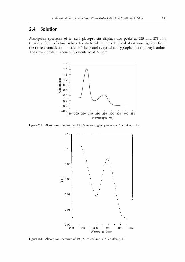
2.4 Solution
Absorption spectrum of α1-acid glycoprotein displays two peaks at 225 and 278 nm(Figure 2.3). This feature is characteristic for all proteins. The peak at 278 nm originates fromthe three aromatic amino acids of the proteins, tyrosine, tryptophan, and phenylalanine.The ε. for a protein is generally calculated at 278 nm.
1.6
Abs
orba
nce
180 200 220 240 260 280 300
Wavelength (nm)
320 340 360
1.4
1.2
1.0
0.8
0.6
0.4
0.2
−0.0
− 0.2
Figure 2.3 Absorption spectrum of 13 μM α1-acid glycoprotein in PBS buffer, pH 7.
0.12
0.10
0.08
0.06
0.04
0.02
0.00200 250 300
Wavelength (nm)350 400 450
OD
Figure 2.4 Absorption spectrum of 19 μM calcofluor in PBS buffer, pH 7.

18 Principles and Applications of Fluorescence Spectroscopy
Absorption spectrum of Calcofluor displays two peaks, one at 242 nm (clearly observedat high concentrations) and the second at 349 nm (Figure 2.4) We notice that both proteinand Calcofluor absorb between 190 and 315 nm. At higher wavelengths, only Calcofluorabsorbs, so in order to determine ε for Calcofluor, one should work at wavelengths whereCalcofluor only absorbs. The best wavelength will be at the peak equal to 349 nm. In thefollowing experiment, we calculate the value of ε at 352.7 nm.
Plotting the optical density as a function of the Calcofluor concentration yields a linearplot with a slope equal to the product (lε) (Figure 2.5). For a cuvette path length l equal to1 cm, the slope is equal to ε, expressed in mg−1 l cm−1. Multiplying the value of ε. by theprotein’s molecular weight yields an ε. expressed in mM−1 cm−1. The value of ε. calculatedfrom the slope is equal to 4.65443 g−1 l cm−1 or 4387.76 M−1 cm−1.
In presence of 10 μM α1-acid glycoprotein, a value of ε. equal to 4.15921 g−1 l cm−1 or3920 M−1 cm−1 is obtained. The value of ε. for bound Calcofluor White is around 9% lowerthan that of free Calcofluor in solution.
1.2
1.0
0.8
0.6
0.4
0.2
0.0
−0.2
OD
−0.05 0.00 0.05 0.10
[Calocfluror White] (g l−1)
0.15 0.20 0.25
a
b
Figure 2.5 Optical density plots of calcofluor white at 352.7 nm as a function of its concentration in(a) the absence and (b) the presence of 10 μM α1-acid glycoprotein. In the absence of protein, ε =4.65443 g−1 l cm−1 = 4387.76 M−1 cm−1. In the presence of the protein, ε = 4.15921 g−1 l cm−1 =3920 M−1 cm−1. Values of ε are not the same; the value of ε for bound calcofluor white is around 9%lower than that of free calcofluor in solution.
Determination of Calcofluor White Molar Extinction Coefficient Value 19
Modification in the value of ε. is the result of structural reorganization in the vicinityof Calcofluor White. The presence of a protein alters the electronic distribution within theligand, inducing a modification of absorption spectrum properties.
We can evaluate ε. for a protein by counting the number of tryptophans, tyrosines, andcysteines in the protein sequence and then applying Equation (1.1) (Gill and von Hippel1989/1990):
ε(M−1cm−1) = (5560 × nb. of Trp) + (1200 × nb. of Tyr) + (60 × nb. of cys) (2.1)
α1-Acid glycoprotein contains three tryptophans, 11 tyrosines, and five cysteines(Figure 2.2). The value of ε. determined from Equation (2.1) is 30.410 mM−1 cm−1. Thus,the experimental and theoretical values are very similiar.
References
Albani, J.R. (2004) Tertiary structure of human α1-acid glycoprotein (orosomucoid). Straightforwardfluorescence experiments revealing the presence of a binding pocket. Carbohydrate Research 339,607–612.
Albani, J.R. (2006) Progesterone binding to the tryptophan residues of human α1-acid glycoprotein.Carbohydrate Research, 341, 2557–2564.
Albani, J.R. and Plancke, Y.D. (1998 and 1999) Interaction between Calcofluor White andcarbohydrates of α1-acid glycoprotein. Carbohydrate Research 314, 169–175 and 318, 194–200.
Albani, J.R., Sillen, A., Coddeville, B., Plancke, Y.D. and Engelborghs, Y. (1999) Dynamics ofcarbohydrate residues of α1-acid glycoprotein (orosomucoid) followed by red-edge excitationspectra and emission anisotropy studies of Calcofluor White. Carbohydrate Research 322, 87–94.
Albani, J.R., Sillen, A., Plancke, Y.D., Coddeville, B. and Engelborghs, Y. (2000) Interaction betweencarbohydrate residues of α1-acid glycoprotein (orosomucoid) and saturating concentrations ofCalcofluor White. A fluorescence study. Carbohydrate Research 327, 333–340.
Åman, P., McNeil, M., Franzén, L.-E., Darvill, A.G. and Albersheim, P. (1981) Structural elucidation,using h.p.l.c.-m.s. and g.l.c.-m.s., of the acidic polysaccharide secreted by Rhizobium meliloti strain1021∗1,∗2. Carbohydrate Research 95, 263–282.
Andreas S., Heindl, S., Wattky, C., Möller, K. and Rüchel, R. (2000) Diagnosis of pulmonaryaspergillosis using optical brighteners. European Respiratory Journal 15, 407.
Brinkman-Van der Linden, E.C., van Ommen, E.C. and van Dijk, W. (1996) Glycosylation of α1-acidglycoprotein in septic shock: changes in degree of branching and in expression of sialyl Lewis(x)groups. Glycoconjugate Journal 13, 27–31.
Canguly, M. and Westphal, U. (1968, Steroid–protein interactions. XVII. Influence of solventenvironment on interaction between human α1-acid glycoprotein and progesterone. Journal ofBiological Chemistry 243, 6130–6139.
Chiu, K.M., Mortensen, R.F., Osmand,A.P. and Gewurz, H. (1977, Interactions of α1-acid glycoproteinwith the immune system. I. Purification and effects upon lymphocyte responsiveness. Immunology32, 997–1005.
De Ceukeleire, M. and Albani, J.R. (2002) Interaction between carbohydrate residues of α1-acidglycoprotein (orosomucoid) and progesterone. A fluorescence study. Carbohydrate Research 337,1405–1410.
Dente, L., Pizza, M.G., Metspalu, A. and Cortese, R. (1987) Structure and expression of the genescoding for human α1-acid glycoprotein. EMBO Journal 6, 2289–2296.
Doctor Fungus website, Candida endophthalmitis. [WWW document]. URL http://216.239.59.104/search?q=cache:1n8Cng6jaK4J:www.doctorfungus.org/mycoses/human/candida/

20 Principles and Applications of Fluorescence Spectroscopy
Endophthalmitis.htm + clinical + studies, + Calcofluor + white&hl = fr [accessed on 20 March,2006].
Gill, S.C. and von Hippel, P.H. (1989) Calculation of protein extinction coefficients from amino acidsequence data. Analytical Biochemistry 182, 319–326. Erratum in: Analytical Biochememistry 1990,189, 283.
Green, L.C., LeBlanc, P.J. and Didier, E.S. (2000) Discrimination between viable and deadencephalitozoon cuniculi (microsporidian) spores by dual staining with Sytox Green andCalcofluor White M2R. Journal of Clinical Microbiology 38, 3811–3814.
Kirley, T.L., Spargue, E.D. and Halsall, H.B. (1982) The binding of spin-labeled propranolol and spinlabeled progesterone by orosomucoid. Biophysical Chemistry 15, 209–216.
Kute, T. and Westphal, U. (1976) Steroid–protein interactions. XXXIV. Chemical modification ofα1-acid glycoprotein for characterization of the progesterone binding site. Biochimica et BiophysicaActa 420, 195–213.
Mackiewicz, A. and Mackiewicz, K. (1995) Glycoforms of serum α1-acid glycoprotein as markers ofinflammation and cancer. Glycoconjugate Journal 12, 241–247.
Maeda, H. and Ishida, N. (1967) Specificity of binding of hexopyranosyl polysaccharides withfluorescent brightener. Journal of Biochemistry 62, 276–278.
Rattee, I.D. and Greur, M.M. (1974) The Physical Chemistry of Dye Absorption. Academic Press,New York.
Sager, G., Nilsen, O.G. and Jackobsen, S. (1979) Variable binding of propranolol in human serum.Biochemical Pharmacology 28, 905–911.
Schmid, K., Kaufmann, H., Isemura, S. et al. (1973) Structure of α1-acid glycoprotein. The completeamino acid sequence, multiple amino acid substitutions and homology with the immunoglobulins.Biochemistry 12, 2711–2724.
Srinivasan, M. (2004) Fungal keratitis. Current Opinion in Ophthalmology 15, 321–327.Van Dijk, W., Havenaar, E.C. and Brinkman-Van der Linden, E.C. (1995) α1-acid glycoprotein
(orosomucoid): pathophysiological changes in glycosylation in relation to its function.Glycoconjugate Journal 12, 227–233.
York, G.M. and Walker, G.C. (1998) The Rhizobium meliloti ExoK and ExsH glycanases specificallydepolymerize nascent succinoglycan chains. Proceedings of the National Academy of Sciences USA95, 4912–4917.

Chapter 3
Determination of Kinetic Parameters ofLactate Dehydrogenase (LDH)
3.1 Objective of the Experiment
Lactate dehydrogenase (LDH) is an oxidoreductase that catalyzes the conversion of lactateto pyruvate. It consists of four subunits that may be of two different types: M and H(“muscle” and “heart” formerly known as A and B, respectively). Five different isoenzymesare therefore possible, depending on the subunit composition:
• LDH-1 (H4)• LDH-2 (H3M)• LDH-3 (H2M2)• LDH-4 (HM3)• LDH-5 (M4)
LDH-1 and LDH-2 are predominant in the heart, while LDH-4 and LDH-5 predominatein skeletal muscle and liver. The molecular weight of all isoenzymes is 140 kDa.
L(+)-Lactate dehydrogenase is specific for L(+)-lactate and does not react with D(−)-lactate. LDH is used in coupled enzyme assays, for example in the determination of ATPase(Penefsky and Bruist 1984), myokinase (Brolin 1983), and pyruvate kinase (Beutler 1971).It may also be used in the determination of lactate (Noll 1984), pyruvate (Lamprecht andHeinz 1984), and various other metabolites.
Thus, the chemical reaction implying LDH is as follows:
Pyruvate + NADH + H+ 1−→←−2
lactate + NAD+
Students should follow reaction number 1 here. They should follow the disappearancekinetics of NADH with absorption spectrophotometry.
Before entering the laboratory, students should be able to explain a kinetic reaction andto demonstrate how to calculate reaction kinetic constants.
3.2 Absorption Spectrum of NADH
Students should receive a stock solution of NADH with a concentration equal to5 mg ml−1. Since the molecular weight of NADH is 709, the concentration of the stock
22 Principles and Applications of Fluorescence Spectroscopy
solution is
5
709= 7.05 × 10⁻³ M = 7.05 mM
The absorption spectrum of NADH should be obtained by adding 10 μl of the stocksolution to 1.2 ml of phosphate buffer (0.1 M, pH 7.5). The concentration of NADH stocksolution should be calculated at 340 nm using an ε. equal to 6200 M−1 cm−1.
3.3 Absorption Spectrum of LDH
Students should take 0.2 ml of the commercially solution (around 2 mg) and centrifugeit to eliminate the ammonium sulfate solution. The pellet obtained should be dissolved in2 ml of phosphate buffer (0.1 M, pH 7.5). The concentration of the solution should be1 mg ml−1. Plot the absorption spectrum of LDH and measure its concentration at 280 nmusing an extinction coefficient equal to 1 (mg/ml)−1 cm−1.
3.4 Enzymatic Activity of LDH
Students should prepare three stock solutions of pyruvate: 150, 30, and 6 mM. 16.5 mgof pyruvate (MW = 110) dissolved in 1 ml of phosphate buffer, pH 7.5, yields a solutionof 150 mM. Dilution of this solution five times yields a stock solution of 30 mM, and itsdilution 25 times yields a stock solution equal to 6 mM.
In a test tube, add: 170 μl of the NADH stock solution, 100 μl of the 30 mM pyruvatestock solution, the appropriate volume of enzyme and then make up the quantity to 3 mlwith phosphate buffer. Mix slowly then measure the variation of absorbance at 340 nm for2 min. Calculate from the data obtained the specific enzyme activity.
The volumes of LDH added to each 3 ml solution prepared should be as follows: 10, 20,30, 40, and 50 μl.
3.5 Kinetic Parameters
Prepare a stock solution of NADH equal to 11 mM. In a test tube, add 100 μl of theNADH solution, different volumes of pyruvate stock solution, and 40 μl of LDH stocksolution diluted 100 times, and then make up the quantity to 3 ml with phosphate buffer.After mixing the solution, measure the optical density at 340 nm after 2 min reaction. Thepyruvate volumes to be added are shown in Table 3.1.
3.6 Data and Results
The absorbance peak of NADH is at 340 nm. The optical density measured should be 0.37,which yields a stock solution concentration of 7.16 mM. The optical density of LDH at280 nm is 1.1, which yields a stock solution equal to 1.1 mg ml−1.
Determination of Kinetic Parameters of Lactate Dehydrogenase 23
Table 3.1 Volumes of added pyruvate and final concentrations in the test tubes
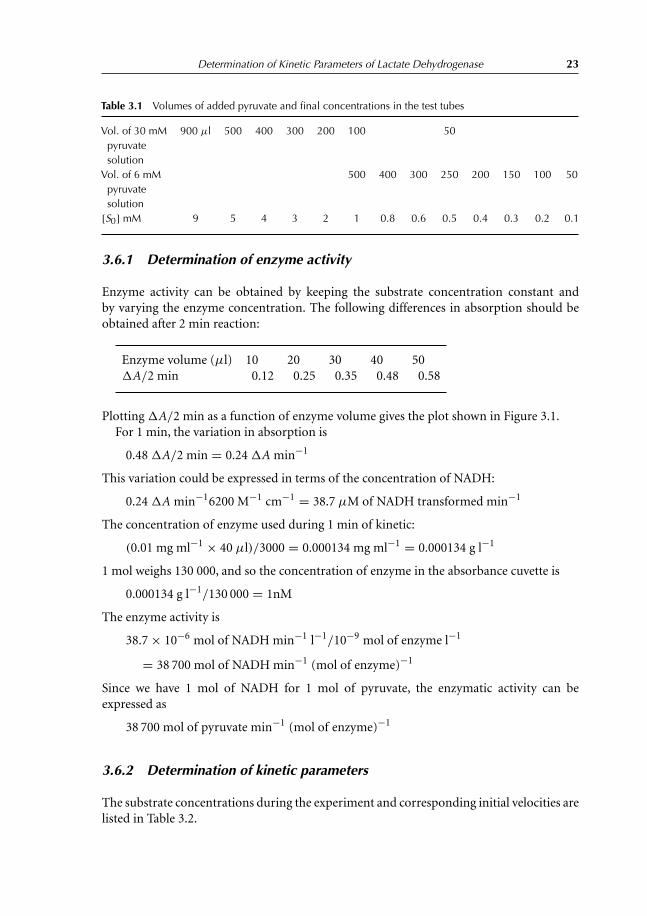
Vol. of 30 mM 900 μl 500 400 300 200 100 50pyruvatesolution
Vol. of 6 mM 500 400 300 250 200 150 100 50pyruvatesolution
[S0] mM 9 5 4 3 2 1 0.8 0.6 0.5 0.4 0.3 0.2 0.1
3.6.1 Determination of enzyme activity
Enzyme activity can be obtained by keeping the substrate concentration constant andby varying the enzyme concentration. The following differences in absorption should beobtained after 2 min reaction:
Enzyme volume (μl) 10 20 30 40 50�A/2 min 0.12 0.25 0.35 0.48 0.58
Plotting �A/2 min as a function of enzyme volume gives the plot shown in Figure 3.1.For 1 min, the variation in absorption is
0.48 �A/2 min = 0.24 �A min−1
This variation could be expressed in terms of the concentration of NADH:
0.24 �A min−16200 M−1 cm−1 = 38.7 μM of NADH transformed min−1
The concentration of enzyme used during 1 min of kinetic:
(0.01 mg ml−1 × 40 μl)/3000 = 0.000134 mg ml−1 = 0.000134 g l−1
1 mol weighs 130 000, and so the concentration of enzyme in the absorbance cuvette is
0.000134 g l−1/130 000 = 1nM
The enzyme activity is
38.7 × 10⁻⁶ mol of NADH min−1 l−1/10−9 mol of enzyme l−1
= 38 700 mol of NADH min−1 (mol of enzyme)−1
Since we have 1 mol of NADH for 1 mol of pyruvate, the enzymatic activity can beexpressed as
38 700 mol of pyruvate min−1 (mol of enzyme)−1
3.6.2 Determination of kinetic parameters
The substrate concentrations during the experiment and corresponding initial velocities arelisted in Table 3.2.

24 Principles and Applications of Fluorescence Spectroscopy
Figure 3.1 Optical density variation at 340 nm for NADH in the presence of different LDH concentrations.
Table 3.2 Values of pyruvate concentrations in the test tubes, and corresponding velocities
[S0] mM 9 5 4 3 2 1 0.8 0.6 0.5 0.4 0.3 0.2 0.1
Vo�A/2 min 0.385 0.48 0.49 0.545 0.55 0.52 0.465 0.425 0.41 0.355 0.355 0.25 0.15
0.49 0.38
Plotting �A/2 min as a function of [S0] gives the graph displayed in Figure 3.2. At excessconcentrations of pyruvate, a velocity decrease can be observed. Kinetic parameters of thereaction can be obtained by plotting the reverse data, i.e., (1/vo vs. 1/[S0]).
The inverse of the maximum velocity Vmax is obtained at the intersection of the plot withthe y-axis (Figure 3.3). This yields a value of Vmax equal to
1/1.43 = 0.7 �A/2 min
Expressed in 1 min and in terms of the NADH concentration, Vmax is
0.7/(6200 M−1 cm−1 × 2) = 5.6 × 10⁻⁵ M min−1

Determination of Kinetic Parameters of Lactate Dehydrogenase 25
0.6
0.5
0.4
0.3
ΔA/2
min
0.2
0.10 2 4
[Pyruvate] (mM)
6 8 10
Figure 3.2 Variation in velocity for NADH formation as a function of pyruvate concentration.
The inverse of the Michaelis constant Km is obtained at the intersection of the plot withthe x-axis. This yields a value of
1/2.7 = 0.37 mM
The catalytic constant kcat is equal to the ratio Vmax/[E0]. Thus, we have to calculate theenzyme concentration in the cuvette. The concentration of the enzyme stock used for theexperiment is 0.011 mg ml−1. We put 40 μl of 10−2 mg ml−1 enzyme in 3 ml.
The enzyme concentration in the experimental solution is
(0.011 mg ml−1 × 40 μl)/3000 μl = 1.47 × 10⁻⁴ mg ml−1 = 1.47 × 10⁻⁴ g l−1
1 mol weighs 130 000 g. The enzyme concentration should be expressed as the number ofmoles dissolved in 1 l of solution:
[E0] = 1.47 × 10⁻⁴ g l−1
130 000 g= 1.13 × 10⁻⁹ mol l−1
kcat = Vm/[E0] = 5.6 × 10⁻⁵ M min−1/10−9 mol = 56 000 min−1
= 933 s−1 by the tetramer of LDH.

26 Principles and Applications of Fluorescence Spectroscopy
Figure 3.3 Inverse plot of the velocity of disappearance of NADH as a function of pyruvate concentration.
3.7 Introduction to Kinetics and the Michaelis–Menten Equation
3.7.1 Definitions
a. The enzyme active site is composed of the amino acids that interact with the substrate.b. The active site of an enzyme contains two sites: substrate binding and catalytic sites.c. The catalytic site acts on the substrate to transform it to one or many products.d. Enzymes are not modified structurally before and after the reaction, act in small
quantities, and do not modify the equilibrium of a reversible reaction. They acceleratethe reaction rate without disturbing the final equilibrium (Figure 3.4).
3.7.2 Reaction rates
The reaction rate is measured by quantifying the product formed under the enzyme actionor the substrate transformed in one unit time.
The molecular activity of an enzyme is the number of substrate molecules transformedin 1 min by one enzyme molecule under optimal conditions of temperature and pH.

Determination of Kinetic Parameters of Lactate Dehydrogenase 27
Eactivation
Ei
EfProducts
Time
Energy of transition
Reactants
In the presence of a chemical catalyzer
In the presence of an enzyme
Figure 3.4 Activation energy of a biological reaction with time in the absence and presence of a chemicalcatalyzer and an enzyme.
3.7.2.1 Zero-order kinetics
This concerns a reaction where the quantity of substrate transformed per time unit isconstantly independent of its concentration.
−dS
dt= k (3.1)
where S is the substrate concentration at a certain time t . The minus sign indicates that thesubstrate concentration is decreasing:
−dS = k dt (3.2)∫−dS =
∫k dt (3.3)
−S = kt + cte (3.4)
At t = 0, cte = −S0, which is the substrate concentration at the beginning of the reaction.Equation (3.4) can be written as
S = −kt + S0 (3.5)
Plotting S as a function of time t yields a linear graph with a slope equal to −k and anintercept at the y-axis equal to S0.
The same analysis can be done by following the variation in product concentration:
dP
dt= k (3.6)∫
dP =∫
k dt (3.7)
P = kt + cte (3.8)
At t = 0, cte = 0.
P = kt (3.9)
The units of k are M s−1.

28 Principles and Applications of Fluorescence Spectroscopy
Time
S
or
PP = f (t )
So Slope = +k
Slope = −k
Figure 3.5 Variation of substrate and product concentrations with time for a zero-order kinetics reaction.
Plotting P as a function of time yields a line that begins at zero with a slope of k (seeFigure 3.5).
3.7.2.2 First-order kinetics
This concerns a reaction where the quantity of substrate transformed per unit timeis proportional to the quantity of the substrate present in solution at the time of themeasurement.
The rate of disappearance of the substrate decreases constantly.
Ak−→ B (3.10)
v = k[A] = −d[A]dt
= d[B]dt
(3.11)
k = v/[A], which means that the dimensions of k are: M s−1/M = s−1.From the definition of the first-order kinetics, one can write:
−dS
dt= kS (3.12)
−dS
S= k dt (3.13)∫
−(dS/S) =∫
k dt (3.14)
− ln S = kt + cte (3.15)
At t = 0, cte = − ln S0. Thus, Equation (3.15) can be written as
− ln S = kt − ln S0 (3.16)

Determination of Kinetic Parameters of Lactate Dehydrogenase 29
ln S
ln S0
Slope = − k
Time
Figure 3.6 Determination of the kinetic constant of a first-order kinetics reaction.
or
ln S = −kt + ln S0 (3.17)
Plotting ln S as a function of t yields a straight line with a slope equal to −k and a y-interceptequal to ln S0 (Figure 3.6).
Equation (3.17) can be modified and written as:
lnS
S0= −kt (3.18)
S
S0= e−kt (3.19)
S = S0e−kt (3.20)
Thus, S decreases exponentially with time. When S = S0/2, we obtain
ln1
2= −kt1/2 (3.21)
or
ln 2 = kt1/2 (3.22)
t1/2 = 0.693/k (3.23)
t1/2 is the half-life of the kinetic reaction.
3.7.2.3 Substrate-to-product transformation in the presence of enzyme
The role of the enzyme in these types of reactions is to accelerate the rate of productformation. However, the substrate possesses a binding site on the enzyme, and so in order

30 Principles and Applications of Fluorescence Spectroscopy
to transform the substrate to a product, an enzyme–substrate complex is formed. Theformation of the product follows the following scheme:
E + Sk1−→←−
k−1
ESk2−→ E + P (3.24)
where ES is the intermediate complex (the Michaelis–Menten complex), and k2 is thecalalytic constant. Product formation occurs from the intermediary complex ES. Thus, thevelocity, v , of the product formation follows a first-order kinetic rule:
v = k2[ES] (3.25)
Quantifying [ES] is difficult, so it should be replaced with other known values.The rate of formation of ES is
d[ES]dt
= k1[Sf ][Ef ] (3.26)
where [Sf ] and [Ef ] are the concentrations of free substrate and enzyme, respectively. Wecan replace [Ef ] by ([E0] − [ES]). Equation (3.26) can be written as
d[ES]dt
= k1[Sf ]([E0] − [ES]) (3.27)
The rate of disappearance of [ES] is
−d[ES]dt
= k2[ES] + k−1[ES] (3.28)
The formation rate of ES is equal to its disappearance rate:
k1[Sf ]([E0] − [ES]) = k2[ES] + k−1[ES] (3.29)
k1[Sf ][E0] − k1[Sf ][ES] = k2[ES] + k−1[ES] (3.30)
k1[Sf ][E0] = k1[Sf ][ES] + k2[ES] + k−1[ES] (3.31)
k1[Sf ][E0] = [ES](k1[Sf ] + k−1 + k2) (3.32)
[ES] = k1[Sf ][E0]k1[Sf ] + k2 + k−1
(3.33)
Dividing both the numerator and denominator by k1 yields
[ES] = [Sf ][E0][Sf ] + (k2 + k−1)/k1
(3.34)
(k2 + k−1)/k1 can be replaced by a constant Km, called the Michaelis–Menten complex:
[ES] = [Sf ][E0][Sf ] + Km
(3.35)
The velocity, v , of the product formation is
v = k2[ES] (3.36)

Determination of Kinetic Parameters of Lactate Dehydrogenase 31
v
Vmax
Vmax/2
Km [S]
Figure 3.7 Schematic representation of the Michaelis–Menten equation.
Thus, combining Equations (3.35) and (3.36) yields:
v = k2[Sf ][E0][Sf ] + Km
(3.37)
For simplification, one could consider that the concentration of bound substrate is toosmall compared to the added substrate [S], and so in Equation (3.37), we can replace [Sf ]by [S].
v = k2[S][E0][Sf ] + Km
(3.38)
Equation (3.38) is known as the Michaelis–Menten equation. We have three constantparameters, k2, [E0], and Km. The two variables are [S] and v . When [S] = 0, v = 0.When [S] → ∞, v → k2[E0] = Vmax. At infinite or high substrate concentrations, v tendsto reach a maximum value Vmax (Figure 3.7).
If the value of Vmax is not reached, plotting 1/v vs. 1/[S] yields a straight line whichintercepts the x-axis at 1/Km and the y-axis at 1/Vmax.
3.7.2.4 Units of the measured parameters and constants
Equation (3.34) shows clearly that the units of Km are those of the substrate, in moles or M.
v = k2[ES] ⇒ k2 = v
[ES] = M s−1
M= s−1 (3.39)
Km = k2 + k−1
k1(3.40)
The units of k2 and k−1 are identical, in s−1.
k1 = k2 + k−1
Km= M−1 s−1 (3.41)
The dimensions of Vmax are identical to those of v , i.e., M s−1.

32 Principles and Applications of Fluorescence Spectroscopy
3.7.2.5 Relationship between Km and the dissociation constant Kd of thecomplex ES
Kd = [Sf ][Ef ][ES] = [Sf ]([E0] − [ES])
[ES] (3.42)
⇒ Kd[ES] = [Sf ][E0] − [ES][Sf ] (3.43)
⇒ Kd[ES] + [ES][Sf ] = [Sf ][E0] (3.44)
⇒ [ES][Sf + Kd] = [Sf ][E0] (3.45)
⇒ [ES] = [Sf ][E0]Kd + [Sf ] (3.46)
With the Michaelis constant, we have the following equation:
[ES] = [Sf ][E0]Km + [Sf ] (3.47)
Equations (3.46) and (3.47) are equal, and so Km is apparently equal to Kd of ES. However,under which conditions does this apply?
Km = k2 + k−1
k1(3.48)
If k−1 >> k2, then
E + Sk1−→←−
k−1
ES
is favored compared to product formation. In this case, we have
Km = k−1
k1(3.49)
Also, in this case, we can write
k1[Sf ][Ef ] = k−1[ES] (3.50)
⇒ Kd = [Sf ][Ef ][ES] = k−1
k1(3.51)
Thus, Km and Kd are equal only if k−1 � k2.
References
Beutler, E. (1971) Red Cell Metabolism, A Manual of Biochemical Methods, pp. 56–68. Grune & StrattonNew York.
Brolin, S.E. (1983) Adenylate kinase (myokinase): UV-method. In: H.U. Bergmeyer (ed.), Methods ofEnzymatic Analysis (3rd edn), Vol. 3, pp. 540–545. Verlag Chemie, Weinheim, Federal Republic ofGermany.

Determination of Kinetic Parameters of Lactate Dehydrogenase 33
Lamprecht, W. and Heinz, F. (1984) Pyruvate. In: H.U. Bergmeyer (ed.), Methods of Enzymatic Analysis(3rd edn), Vol. 6, pp. 555–561. Verlag Chemie, Weinheim.
Noll, F. (1984) L(+)-lactate. In: H.U. Bergmeyer (ed.), Methods of Enzymatic Analysis (3rd edn), Vol. 6,pp. 582–528. Verlag Chemie, Weinheim.
Penefsky, H.S. and Bruist, M.F. (1984) Adenosinetriphosphatases. In: H.U. Bergmeyer (ed.), Methodsof Enzymatic Analysis (3rd edn), Vol. 4, pp. 324–328. Verlag Chemie, Weinham.

Chapter 4
Hydrolysis of p-Nitrophenyl-β-D-Galactosidewith β-Galactosidase from E. coli
4.1 Introduction
β-Galactosidase is a tetrameric enzyme that consists of identical subunits with a molecularmass of 135 000. Amino-acid analysis indicates approximately 1170 residues per subunit.Each monomer is composed of five compact domains and a further 50 additional residuesat the N-terminal end. Within the cell, β-galactosidase cleaves lactose to form glucose andgalactose. The latter is exchanged with lactose via a lactose–galactose antiport system. Thecomposition and structure of the cell wall change continuously during plant development.Thus, the cell wall is dynamic, not static. Plant cell walls consist of cellulose microfibrilscoated by xyloglucans and embedded in a complex matrix of pectic polysaccharides (Talbottand Ray 1992; Carpita and Gibeaut 1993). Plant development involves a coordinatedseries of biochemical processes that, among other things, result in the biosynthesis anddegradation of cell-wall components. Enzymes such as β-galactosidase and α-arabinosidaseplay a role in the cross-linking of pectins and cell-wall proteins by catalyzing theformation of phenolic-coupling activity. The enzymes hydrolyze corresponding phospho-p-nitrophenylderivatives (α-L-arabinofuranoside and β-D-galactopyranoside, respectively)into p-nitrophenol (PNP) (Figure 4.1) that absorbs at 410 nm. Thus, it is possible tofollow the evolution of plant development by quantifying the PNP formed, as shown in astudy performed by Stolle-Smits et al. (1999) by following the absorption of PNP at 420 nm(4.8×10³ M−1 cm−1). For more information on the properties of β-galactosidase, studentscan look to the following link:
http://www.mpbio.com/product_info.php?cPath=491_1_12&products_id=150039&depth=nested&keywords=beta%20galactosidase
The purpose of the present experiments is to characterize kinetics parameters ofp-nitrophenyl-β-D-galactoside hydrolysis with β-galactosidase. Students will find out howto use absorption spectroscopy to study enzymatic properties of an enzyme (see alsoMurata et al. 2003). Before entering the lab, students should be able to explain theBeer–Lambert–Bouguer law and the basics of enzymology.

Hydrolysis of p-Nitrophenyl-β-D-Galactoside 35
OOH
OH
OH
CH2 OH
H
O NO2
OH
N+
O
−O
OOH
OH
OH
CH2OH
OH
H
+p-Nitrophenyl-β-D-galactosidase
+H2O
�-Galactosidase
N+
Figure 4.1 Reaction describing the hydrolysis of p-nitrophenyl-β-D-galactosidase into p-nitrophenol andβ-D-galactose.
4.2 Solutions to be Prepared
• β-Galactosidase is purchased as a suspension in 60% saturation of ammonium sulfatesolution. The solution given to students corresponds to 1.5 ml of the purchased proteindissolved in 500 ml of buffer pH 7. The diluted solution is stable at the maximum 1 weekat 4◦C.
• 1 mM heteroside solution: Dissolve 0.03 g of p-nitrophenyl-β-D-galactosidase in 100 mlof distilled water containing 10 mg of sodium azide.
• 10 mM heteroside solution: Dissolve 0.3 g of p-nitrophenyl-β-D-galactosidase in 100 mlof distilled water containing 10 mg of sodium azide.
• Stock solution of paranitrophenol at 10−6 mol ml−1: Dissolve 139.11 mg in 1 l ofdistilled water containing 1 drop of concentrated HCL solution.
• 1 M sodium carbonate solution: Dissolve 106 g in 1 l of distilled water.• Buffers from pH 2 to 12: Buffers can be phosphate or Tris. Add 0.1 g of sodium azide to
each 1 l of buffer prepared.
All the experiments are performed in test tubes of internal diameter equal to 1.5 cm.
4.3 First-day Experiments
During the first day, students will discover the absorption properties of PNP and willdetermine the optimal temperature and pH of β-galactosidase.
4.3.1 Absorption spectrum of PNP
Plot an absorption spectrum from 340 to 480 nm of 0.1 ml of 1 mM PNP solution mixedwith 4.9 ml of Na2CO3vs 0.1 ml of water mixed to 4.9 ml of Na2CO3. Calculate ελ max.

36 Principles and Applications of Fluorescence Spectroscopy
0.6
0.5
0.4
0.3
OD
0.2
0.1
0.0320 340 360 380 400
Wavelength (nm)
420 440 460 480 500
Figure 4.2 Absorption spectrum of paranitrophenol in basic medium.
The absorption spectrum of PNP (Figure 4.2) displays a maximum around 405 nm.The optical density (OD) recorded at this wavelength is slightly higher than that recordedat 410 nm. The value of ε. at 405 nm and at any wavelength can be obtained from theBeer–Lambert–Bouguer law:
ε405 nm = OD405 nm
cxl= 0.59
(10−3 M/50) × 1.5 cm= 19 666 M−1 cm−1
4.3.2 Absorption of PNP as a function of pH
Measure the OD at the absorption maximum (in our case, 405 nm) of 0.5 ml of 1 mM PNPmixed to 4.5 ml buffer vs. 0.5 ml water mixed with 4.9 ml buffer. Experiments should beperformed with buffers at different pHs (from 2 to 10). Then, plot the measured ODs as afunction of pH. The plot is displayed in Figure 4.3.
4.3.2.1 Conclusion
PNP absorbs only in the deprotonated form, and so in order to observe its formation afterthe enzymatic reaction, we need to increase the pH in the test tube. This can be achieved by

Hydrolysis of p-Nitrophenyl-β-D-Galactoside 37
2.0
1.5Protonated form:no absorbance
Mixture of protonatedand deprotonatedforms
Deprotona-ted form
1.0
0.5
OD
0.00 2 4 6 8 10
pH
Figure 4.3 Optical density of PNP at 405 nm at different pHs.
adding Na2CO3 to the enzyme–substrate solution. Addition of Na2CO3 helps to stop theenzymatic reaction and allows the OD of the formed PNP to be read.
4.3.3 Internal calibration of PNP
The purpose of this experiment is to determine up to which PNP concentration, the Beer–Lambert–Bouguer law is still linear. In fact, this law cannot be applied when the opticalsaturation of the photomultiplier is reached and/or when the chromophore aggregates.Each spectrophotometer cannot count more than a precise number of photons. Whenthis number is reached, the OD given by the spectrophotometer will be the highest, and thephotomultiplier is saturated. Beyond the“saturation concentration,”the spectrophotometerwill always give the same OD that corresponds to that of saturation.
Also, Beer–Lambert–Bouguer law can no longer be applied because of the chromophoreitself. At high concentrations, aggregation could occur. In this case, we are going to havetwo values of ε, corresponding to low and high concentrations. Plotting OD as a functionof macromolecule concentration yields two plots with two different ε. values.
Prepare two series of test tubes. In the first series, add 0, 0.5, 1, 1.5, and 2 ml of the 0.1 mMPNP solution. In the second series, add 0.2, 0.5, 1, 1.5, and 2 ml of the 1 mM PNP solution.Make up the solution to 2 ml with distilled water, add 3 ml of Na2CO3, and mix well.

38 Principles and Applications of Fluorescence Spectroscopy
2.0
OD
0.0
0.2
0.4
0.6
0.8
1.0
1.2
1.4
1.6
1.8
0.0 0.1 0.2 0.3 0.4
[PNP] (�M)
Figure 4.4 Plots of the optical density of PNP as a function of PNP concentration measured at 405(squares) and 430 nm (circles).
Measure the ODs at 405 nm and 430 nm vs. the blank solution where PNP is replaced bywater.
Plot the OD as a function of PNP concentration in the tube at the two wavelengthsand determine for each wavelength the maximum PNP concentration at which the Beer–Lambert–Bouguer law is still linear.
The graph (Figure 4.4) shows that the linearity of the Beer–Lambert–Bouguer law canbe applied up to ODs equal to around 1.6. This yields a PNP concentration of 0.0675 and0.1 mM at 405 and 430 nm, respectively. The molar extinction coefficient at 430 nm is lowerthan that at 405, and it can be calculated from the data of Figure 4.2. In fact, the value of ε
at 430 nm is 16 000 M−1 cm−1.Plots obtained show that above 0.07 mM, OD continues to increase, indicating that PNP
is probably aggregating. The aggregate does not have the same absorbance properties as themonomer.
4.3.3.1 Conclusion
In order to perform qualitative and quantitative studies with β-galactosidase, we shouldwork in experimental conditions such that only the monomer of PNP is detected. Also, one

Hydrolysis of p-Nitrophenyl-β-D-Galactoside 39
should work below the detection limit of the spectrophotometer; otherwise we are going toread the same OD at all high concentrations of PNP present in solution.
One should work at an enzyme concentration that yields sufficient PNP to be observedwith the spectrophotometer but not in excess, so as to avoid aggregation and/or ODsaturation.
Figure 4.4 indicates also that working at 430 nm allows the detection of higher PNPconcentrations than when the experiment is performed at 405 nm. However, in both cases,the ODs measured by the end of the hydrolysis should be lower than 1.6.
4.3.4 Determination of β-galactosidase optimal pH
Experiments should be performed using pH buffers going from 2 to 10. Add to a test tube:0.5 ml of 1 mM heteroside, 1 ml of buffer, and 2 ml of enzyme. Then, mix with the vortexand allow to incubate for 3 min. Finally, add 3 ml of Na2CO3.
In the blank tube, add the 3 ml of Na2CO3 before adding the enzyme. Plot the OD at405 nm as a function of pH.
The result (Figure 4.5) shows that the optimum pH of the enzyme is 7. Thus, at thispH, the activity of β-galactosidase is the most important. Therefore, in the following
Figure 4.5 Determination of the optimum pH of β-galactosidase.

40 Principles and Applications of Fluorescence Spectroscopy
experiments, pH 7 buffer will be used. Adding Na2CO3 induces a high pH, which denaturesthe enzyme and stops hydrolysis. At the same time, it will be possible to read the OD of thePNP formed.
4.3.5 Determination of β-galactosidase optimal temperature
Enzyme activity is temperature-dependent. Parameters such as temperature and pH affectenzyme structure. Enzyme activity is most important in its native form, modifying thenative structure with the temperature, or the pH decreases enzyme activity. In the nativeform, an enzyme is most active at its optimal pH and temperature. Physiological propertiesof macromolecules are modified with temperature variation. Molecules will lose theirphysiological properties only when they reach a temperature that denatures their molecularstructure. However, one should be cautious when studying folding and/or unfolding ofproteins, since the different regions of the proteins do not behave similarly with temperature.In fact, denaturation of an enzyme active site with temperature could be more difficult thanother regions of the protein.
The optimal pH of β-galactosidase was determined at ambient temperature, 20◦C.However, this temperature is not necessarily the optimal one. Hydrolysis of the heterosideshould be performed at the following temperatures: 0◦C, 10◦C, 20◦C, 30◦C, 40◦C, 50◦C,60◦C, and 100◦C.
In a test tube, mix 0.5 ml of 1 mM heteroside and 1 ml of pH 7 buffer. Then, keepthe test tube for 5 min at the temperature of the experiment. Then, add 0.5 ml of theenzyme solution without removing the test tube from its position, mix the whole solutionslowly, and allow the hydrolysis to continue for 5 min. Then, add 3 ml of Na2CO3. A blanktube is prepared by adding Na2CO3 before the enzyme. Read the OD at 405 nm at roomtemperature, and then plot it as a function of temperature.
The data (not shown) indicate that the optimal temperature is 35◦C. However, in orderto decrease the enzyme activity slightly, the hydrolysis experiments can be performed at25◦C.
4.4 Second-day Experiments
Students will learn how to measure enzyme kinetics and how to determine proteinconcentration using Bradford’s method (Bradford, 1976).
4.4.1 Kinetics of p-nitrophenyl-β-D-galactoside hydrolysis withβ-galactosidase
Add to 12 test tubes: 0.5 ml of 1 mM heteroside and 1.9 ml of pH 7 buffer. Mix with thevortex and maintain the tubes for 5 min at 25◦C. Then, add 0.1 ml of enzyme solution, mixwith the vortex, and put the tubes back at 25◦C. After 1, 2, 3, 4, 5, 6, 8, 10, 20, 30, 45 and60 min, add 3 ml of Na2CO3. Read the OD at 405 nm vs a blank tube where Na2CO3 wasadded before the enzyme. Then, plot the OD as a function of time (Figure 4.6). Check thatthe measured ODs correspond to the linear part of the plot of Figure 4.4.

Hydrolysis of p-Nitrophenyl-β-D-Galactoside 41
1.6
1.4
1.2
1.0
OD
0.0
0.4
0.2
0.6
0.8
0 10 20 30 40 50 60
Time (min)
Figure 4.6 Kinetics of p-nitrophenyl-β-D-galactoside hydrolysis with β-galactosidase.
First, we can see that the measured ODs fit within the linear part of the plot of Figure 4.4.The ODs correspond to PNP resulting from p-nitrophenyl-β-D-galactoside hydrolysis.From the slope of the linear part of the kinetics, we can calculate the hydrolysis velocity, i.e.,the PNP concentration formed per minute.
At 15.5 and 5 min, the corresponding ODs are 1.2 and 0.4. Thus, the slope of the linearpart is equal to
Slope = OD1 − OD2
t1 − t2= 1.2 − 0.4
15.5 − 5.0= 0.8
10.5= 7.62 × 10⁻² min−1 (4.1)
Knowing the path length and the molar extinction coefficient, we can calculate theequivalent concentration of PNP observed:
[PNP] = 7.62 × 10⁻²
19 666 M−1 cm−1 × 1.5 cm= 2.58 × 10⁻⁶ mol l−1 min−1 (4.2)
The ODs shown in Figure 4.6, and so the measured concentrations of PNP are thoseobtained in 5.5 ml of final solution after the addition of Na2CO3. The real ODs and thereal concentration of PNP formed are higher since hydrolysis was performed in 2.5 ml.
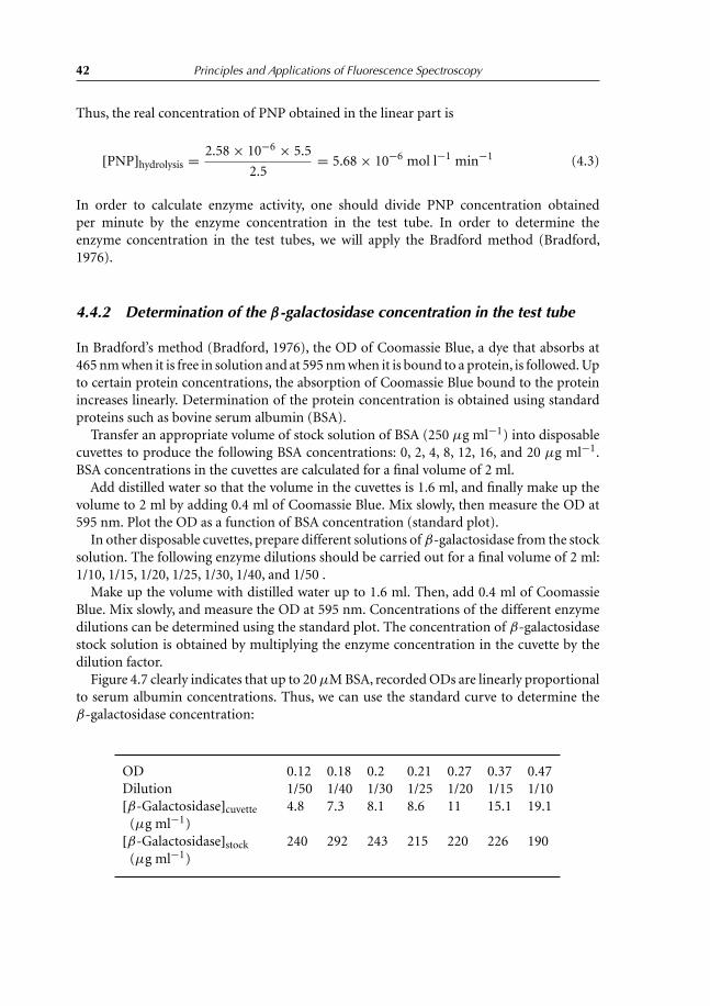
42 Principles and Applications of Fluorescence Spectroscopy
Thus, the real concentration of PNP obtained in the linear part is
[PNP]hydrolysis = 2.58 × 10−6 × 5.5
2.5= 5.68 × 10⁻⁶ mol l−1 min−1 (4.3)
In order to calculate enzyme activity, one should divide PNP concentration obtainedper minute by the enzyme concentration in the test tube. In order to determine theenzyme concentration in the test tubes, we will apply the Bradford method (Bradford,1976).
4.4.2 Determination of the β-galactosidase concentration in the test tube
In Bradford’s method (Bradford, 1976), the OD of Coomassie Blue, a dye that absorbs at465 nm when it is free in solution and at 595 nm when it is bound to a protein, is followed. Upto certain protein concentrations, the absorption of Coomassie Blue bound to the proteinincreases linearly. Determination of the protein concentration is obtained using standardproteins such as bovine serum albumin (BSA).
Transfer an appropriate volume of stock solution of BSA (250 μg ml−1) into disposablecuvettes to produce the following BSA concentrations: 0, 2, 4, 8, 12, 16, and 20 μg ml−1.BSA concentrations in the cuvettes are calculated for a final volume of 2 ml.
Add distilled water so that the volume in the cuvettes is 1.6 ml, and finally make up thevolume to 2 ml by adding 0.4 ml of Coomassie Blue. Mix slowly, then measure the OD at595 nm. Plot the OD as a function of BSA concentration (standard plot).
In other disposable cuvettes, prepare different solutions of β-galactosidase from the stocksolution. The following enzyme dilutions should be carried out for a final volume of 2 ml:1/10, 1/15, 1/20, 1/25, 1/30, 1/40, and 1/50 .
Make up the volume with distilled water up to 1.6 ml. Then, add 0.4 ml of CoomassieBlue. Mix slowly, and measure the OD at 595 nm. Concentrations of the different enzymedilutions can be determined using the standard plot. The concentration of β-galactosidasestock solution is obtained by multiplying the enzyme concentration in the cuvette by thedilution factor.
Figure 4.7 clearly indicates that up to 20 μM BSA, recorded ODs are linearly proportionalto serum albumin concentrations. Thus, we can use the standard curve to determine theβ-galactosidase concentration:
OD 0.12 0.18 0.2 0.21 0.27 0.37 0.47Dilution 1/50 1/40 1/30 1/25 1/20 1/15 1/10[β-Galactosidase]cuvette 4.8 7.3 8.1 8.6 11 15.1 19.1
(μg ml−1)[β-Galactosidase]stock 240 292 243 215 220 226 190
(μg ml−1)

Hydrolysis of p-Nitrophenyl-β-D-Galactoside 43
Figure 4.7 Optical density of Coomassie Blue as a function of serum albumin concentrations.
The mean value of the β-galactosidase stock solution is 232 μg ml−1. The β-galactosidase concentration used in the kinetics experiment is (0.1 ml × 232 μg ml−1):2.5 ml = 9.28 μg ml−1. The activity of β-galactosidase is
[PNP]hydrolysis
[Enzyme] = 5.68 × 10⁻⁶mol l−1 min−1
9.28 × 10⁻³g l−1 = 0.612 × 10−3
= 6.12 × 10⁻⁴ mol of PNP min−1 g−1enzyme (4.4)
4.4.2.1 Suggested experiment
We suggest here that students determine β-galactosidase activity by performing hydrolysisfor a constant time and at different enzyme concentrations.

44 Principles and Applications of Fluorescence Spectroscopy
4.5 Third-day Experiments
Students should be able to describe the theory of Michaelis–Menten before enteringthe lab.
4.5.1 Determination of Km and Vmax of β-galactosidase
The instructor should give the students two stock solutions of p-nitrophenyl-β-D-galactoside (1 and 10 mM). Students should then prepare the following heterosideconcentrations in a final volume of 2 ml: 0.1, 0.25, 0.5, 0.75, 1, 2.5, 5, 7.5, and 10 mM.
From each of these new stock solutions, prepare the following test tubes. First, add 0.5ml of heteroside solution, then 1.2 ml of pH 7 buffer, and finally 0.3 ml of enzyme solution.Mix slowly and then keep the hydrolysis reaction going for 3 min at 20◦C. Then, add 3 mlof Na2CO3. Measure the ODs vs. a blank where Na2CO3 is added before the enzyme. Fromthe plot, OD vs. [p-nitrophenyl-β-galactoside] (Figure 4.8), calculate Vmax and Km. Fromnow on, plot the graphs using the real ODs, i.e., those you should measure in the volume ofhydolysis solution, and not those you measured after addition of 3 ml of Na2CO3.
OD
4
3
2
1
00.0 0.5 1.0 1.5 2.0 2.5
[p-Nitrophenyl-�-D-galactoside] (mM)
Figure 4.8 Optical density variation with the concentration of [p-nitrophenyl-β-galactoside]. The opticaldensities correspond to 2 ml of hydrolysis solution.
The value of Km corresponds to the concentration of substrate where velocity is equal tohalf of Vmax. Km is 0.425 × 10⁻³ mol l−1 = 4.25 × 10⁻⁴ mol l−1. The Michaelis constantgiven in the literature for the PNP hydrolysis with β-D-galactosidase is 4.45 × 10⁻⁴ M. In

Hydrolysis of p-Nitrophenyl-β-D-Galactoside 45
Figure 4.9 Double reciprocal plot of PNP optical density vs. [p-nitrophenyl-β-D-galactoside] at highheteroside concentrations.
order to be sure that at the highest concentration (2.5 mM) of heteroside, the measuredOD corresponds or is very close to the maximum value, we have plotted the inverse graph1/v vs. 1/[p-nitrophenyl-β-galactoside] (Figure 4.9). The value of Vmax obtained uponextrapolation on the y-axis is 3.8, thus clearly indicating that the maximum velocity hasbeen reached.
Vmax can be expressed as the concentration of formed PNP:
Vmax = OD
εxl= 3.75
19 666 × 1.5= 1.27 × 10⁻⁴ mol of PNP l−1min−1 (4.5)
4.5.1.1 Suggested experiment
Students can repeat the last experiment in the presence of two different inhibitorconcentrations to determine its effect on the hydrolysis rate.
4.5.2 Inhibiton of hydrolysis kinetics of p-nitrophenyl-β-D-galactoside
The instructor should give students three stock solutions of inhibitor: 5, 10, and 30 mM.Students are going to prepare two series of six test tubes, containing each of the following
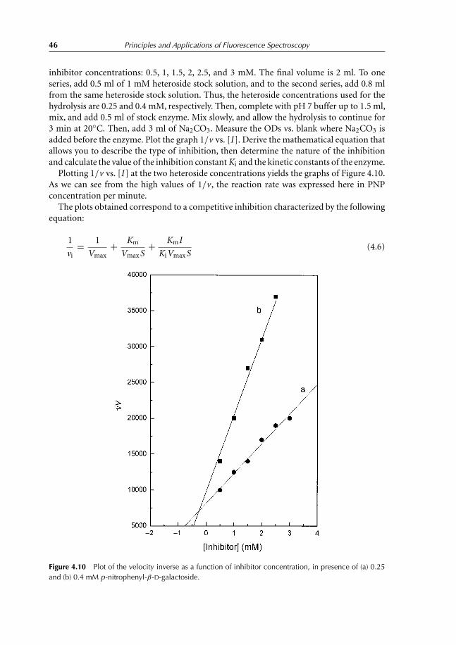
46 Principles and Applications of Fluorescence Spectroscopy
inhibitor concentrations: 0.5, 1, 1.5, 2, 2.5, and 3 mM. The final volume is 2 ml. To oneseries, add 0.5 ml of 1 mM heteroside stock solution, and to the second series, add 0.8 mlfrom the same heteroside stock solution. Thus, the heteroside concentrations used for thehydrolysis are 0.25 and 0.4 mM, respectively. Then, complete with pH 7 buffer up to 1.5 ml,mix, and add 0.5 ml of stock enzyme. Mix slowly, and allow the hydrolysis to continue for3 min at 20◦C. Then, add 3 ml of Na2CO3. Measure the ODs vs. blank where Na2CO3 isadded before the enzyme. Plot the graph 1/v vs. [I ]. Derive the mathematical equation thatallows you to describe the type of inhibition, then determine the nature of the inhibitionand calculate the value of the inhibition constant Ki and the kinetic constants of the enzyme.
Plotting 1/v vs. [I ] at the two heteroside concentrations yields the graphs of Figure 4.10.As we can see from the high values of 1/v , the reaction rate was expressed here in PNPconcentration per minute.
The plots obtained correspond to a competitive inhibition characterized by the followingequation:
1
vi= 1
Vmax+ Km
VmaxS+ KmI
KiVmaxS(4.6)
Figure 4.10 Plot of the velocity inverse as a function of inhibitor concentration, in presence of (a) 0.25and (b) 0.4 mM p-nitrophenyl-β-D-galactoside.

Hydrolysis of p-Nitrophenyl-β-D-Galactoside 47
where vi is the reaction rate in presence of inhibitor I , Ki is the inhibitor constantcorresponding to the dissociation constant of the enzyme–inhibitor complex, and S isthe substrate concentration.
Plotting 1/vi as a function of I , yields a linear plot of slope equal to
Km
KiVmaxS
and a y-intercept equal to
1
Vmax+ Km
VmaxS
When S increases, the slope decreases.When
1
vi= 1
Vmax, I = −Ki
Thus, plotting 1/vi as a function of I for different (two to three) substrate concentrationsyields linear plots that intercept together at a point having as coordinates (−Ki and 1/Vmax).From the graph, we obtain 1/Vmax equal to 7000, i.e., a Vmax equal to 1.42×10⁻⁴ mol min−1
and Ki equal to 0.28 mM.From the y-intercept value, we can calculate Km value. The y-intercepts are equal to 8166
and 10 000 for plot (a) ([heteroside] = 0.4 mM) and plot (b) ([heteroside] = 0.25 mM),respectively. Thus, we have 0.663 × 10⁻⁴ mol l−1 and 1.065 × 10⁻⁴ mol l−1 for plots (a)and (b), respectively.
4.6 Fourth-day Experiments
4.6.1 Effect of guanidine chloride concentration on β-galactosidase activity
Protein denaturation induces a loss of its secondary and tertiary structures. Since the tertiarystructure is responsible for proteins’ physiological properties, its loss induces total proteininactivation. Denaturation occurs in different ways: thermal, pH, urea, guanidine salts(mainly guanidine chloride), organic solvents, and detergents. Denaturation does not occurinstantaneously and depends not only on the nature of denaturing factor or agent but also onthe macromolecule concentration and structure. The most effective denaturant is guanidinechloride. Total loss of the molecules structure occurs at 6 M GndCl. The salt is a strongelectrolyte, which means that it interacts with the protein via electrostatic charges. Proteincharges that maintain the folded structure are neutralized by electrostatic interaction withguanidine chloride, thereby inducing an unfolded protein. Also, interaction of guanidinechloride occurs with amino acids of a protein inner core, thereby inducing an irreversibleunfolded state.
In the following experiment, we will study β-galactosidase denaturation by guanidinechloride following OD of PNP at 405 nm. Enzyme denaturation induces a loss in its activity,which will be observed by the decrease in the OD.
Students should be given a solution of 6 M guanidine. Then, they should prepare thefollowing guanidine chloride stocks: 0, 0.05, 0.1, 0.15, 0.20, 0.25, 0.30, 0.35, 0.40, 0.45,

48 Principles and Applications of Fluorescence Spectroscopy
and 0.50 M. Then, in 11 test tubes each containing 4 ml of stock enzyme, add 1 ml of theguanidine solution stocks. Mix and leave the mixture for 15 min. Then, add 0.25 ml of themixture to test tubes containing 0.5 ml of 10 mM heteroside and 1.75 ml of pH 7 buffer.Mix and allow the reaction to continue for 25 min at 37◦C. Then, add 3 ml of Na2CO3 andmeasure the ODs at 405 nm vs. a blank where Na2 CO3 was added before the enzyme. Finally,plot the corrected OD for the volume (2.5 ml) of hydrolysis and for 1 min as a function ofguanidine chloride concentration in the test tubes. The same experiment should be done at25◦C also.
Derive the mathematical equation that allows you to calculate the equilibrium constantKeq at each guanidine concentration and plot Keq = f ([guanidine]. Finally, determine�G◦′ at each guanidine concentration and plot �G◦′ = f ([guanidine] and �G◦′ = f([Keq]). Calculate from the last graph the value of Keq.
Do the graphs obtained correspond to the theoretical significance of �G◦′ and Keq?Do you obtain the same information from both experiments, at 25 and 37◦C?
4.6.2 OD variation with guanidine chloride
Figure 4.11 displays the OD variation of PNP formed in the presence of different guanidinechloride concentrations. We notice that a loss of total enzyme activity occurs at 8 mMguanidine chloride. The enzyme concentration was small, which explains the total lossof activity at concentrations of guanidine chloride much lower than 6 M. The fact thatOD reaches zero indicates that with 8 mM guanidine, all β-galactosidase present inthe test tube is in a denatured form. In other words, denaturation of the enzyme byguanidine is total and not partial. The denatured structure of β-galactosidase is no longeractive.
The hyperbolic shape of the curve in Figure 4.11 allows a dissociation constant to beobtained for the guanidine-β-galactosidase complex equal to 2.2 mM.
4.6.3 Mathematical derivation of Keq
The absorption values of native and denatured β-galactosidase in the presence of a certainconcentration of guanidine are denoted as An and Ad, respectively. In the presence ofguanidine concentrations where equilibrium exists between the two protein states, therecorded absorbance A(obs) is
A(obs) = An + Ad (4.7)
A(obs) = εNCNl + εDCDl = εN(Co − CD)l + εDCDl (4.8)
where εN and CN are the molar extinction coefficient and concentration of the native form,εD and CD are the molar extinction coefficient and concentration of the denatured form,and Co is the total enzyme concentration in the solution.
A(obs) = εNCol − εNCDl + εDCDl (4.9)
= A(N) + CDl(εD − εN) (4.10)

Hydrolysis of p-Nitrophenyl-β-D-Galactoside 49
Figure 4.11 Activity variation of β-galactosidase (18.5μgml−1) as a function of guanidine concentration.The experiment was performed at 37◦C.
A(N) and A(D) denote enzyme absorptions when it is completely native or denatured.
A(obs) = ANXDCol(εD − εN) (4.11)
where XD is the fraction of the denatured form.
A(obs) = A(N) + XDColεD − XDColεN (4.12)
= A(N) + XDA(D) − XDA(N) (4.13)
= A(N) + XD[A(D) − A(N)] (4.14)
A(obs) − A(N) = XD[A(D) − A(N)] (4.15)
XD = Aobs − AN
AD − AN(4.16)
Keq = CD
CN= XDCo
XNCo= XD
XN(4.17)

50 Principles and Applications of Fluorescence Spectroscopy
Figure 4.12 Plot of Keq as a function of [guanidine]. At high guanidine concentrations, β-galactosidaseis completely denatured, yielding an infinite value of Keq.
XN = 1 − XD = AD − AN − Aobs + AN
AD − AN= AD − Aobs
AD − AN(4.18)
Keq = Aobs − AN
AD − Aobs(4.19)
Thus, it is possible to calculate the equilibrium constant at each guanidine chlorideconcentration using Equation (4.19). Keq = f ([guanidine]) yields the graph shown inFigure 4.12.
How do we interpret the results obtained for the equilibrium constant variation? Let usconsider the following chemical reaction:
aA + bB1−→←−2
cC + dD (4.20)
When the system is in equilibrium, we can write:
Keq = [C]c [D]d
[A]a[B]b(4.21)
If Keq >[C]c [D]d
[A]a[B]b⇒ Keq[A]a[B]b > [C]c [D]d (4.22)

Hydrolysis of p-Nitrophenyl-β-D-Galactoside 51
In this case, reactants are in excess, and the reaction will occur in direction 1.
If Keq <[C]c [D]d
[A]a[B]b⇒ Keq[A]a[B]b < [C]c [D]d (4.23)
In this case, products are in excess, and the reaction will occur in direction 2. The purposeof this displacement, whether in direction 1 or 2, is to reach equilibrium.
If Keq < 1 ⇒ [reactants] > [products]If Keq > 1 ⇒ [reactants] < [products]
In our experiments, although equilibrium between native and denatured forms ofβ-galactosidase exists at all guanidine chloride concentrations, at high concentrations theenzyme will be in one form, denatured, and thus there will be no kinetic equilibrium.
4.6.4 Definition of the standard Gibbs free energy, �G◦′
The Phase Rule describes the possible number of degrees of freedom in a (closed) system atequilibrium, in terms of the number of separate phases and the number of chemical constituentsin the system. It was deduced from thermodynamic principles by J. W. Gibbs in the 1870s.(http://jwgibbs.cchem.berkeley.edu/phase_rule.html)
Measurement of the internal energy of a system requires that we have already defined areference or standard state. This is the state where a component is most stable at normaltemperature and pressure. When �G is measured at the standard conditions, it is denotedas �G◦.
For chemists, the standard conditions of a system are a pressure of 1 atm, a temperatureequal to 25◦C or 298 K, a chemical component concentration of 1 M and consequently apH = 0 (since pH = − log[H+] and [H+] = 1 M).
However, standard conditions in biochemistry and in biology are different, since chemicalreactions in cells occur at around pH 7. Therefore, standard conditions in biochemistrydiffer from those in chemistry, which implies that the standard Gibbs free energy within abiological system is denoted as �G◦′. Standard conditions in biochemistry and biology are:a pH equal to 7 and a constant water concentration that does not appear in the mathematicaldefinition of the equilibrium constant.
4.6.5 Relation between �G◦′ and �G ′
Let us consider the following reaction:
aA + bB1−→←−2
cC + dD (4.24)
The �G◦′ of the reaction is∑�G◦′
(products) −∑
�G◦′(reactants) (4.25)
G ′ = H − TS = U + PV − TS (4.26)

52 Principles and Applications of Fluorescence Spectroscopy
where H , S, U , P , and V are the enthalpy, entropy, internal energy, pressure, and volume ofthe system, respectively.
The first derivative of Equation (4.25) is
dG ′ = dU + P dV + V dP − T dS − S dT (4.27)
dU can be replaced by dQ − P dV where dQ is the variation of heat within the system.Then,
dG ′ = dQ − P dV + V dP − T dS − S dT = dQ + V dP − T dS − S dT (4.28)
dQ = T dS (4.29)
Replacing Equation (4.29) in Equation (4.28) yields
dG ′ = T dS + V dP − T dS − S dT = V dP − S dT (4.30)
At a constant temperature,
dG ′ = V dP (4.31)
For 1 mol of component,
P V = RT (4.32)
or
V = RT/P (4.33)
Combining Equations (4.32) and (4.33) yields
d G ′ = RT
PdP (4.34)
The integral of Equation (4.34) between G◦′and G ′ and Po(1 atm) and P yields
G′∫ G◦′
d G ′ =P∫
Po
RT
PdP (4.35)
G ′ − G◦′ = RT logP
Po= RT log P (4.36)
If we have n mol instead of 1, we have
n G ′ = n G◦′ + nRT log P (4.37)
4.6.6 Relation between �G◦′ and Keq
Let us consider the following reaction:
αA(PA) + βB(PB)−→←− cC(PC ) + dD(PD) (4.38)
∑�G◦′
(products) −∑
�G◦′(reactants) (4.39)
�G ′ = c G ′(C) + d G ′(D) − α G ′(A) − β G ′(B) (4.40)
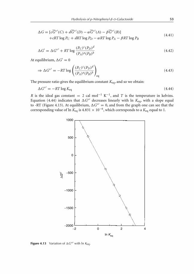
Hydrolysis of p-Nitrophenyl-β-D-Galactoside 53
�G = [c G◦′(C) + d G◦′
(D) − α G◦′(A) − β G◦′
(B)]+cRT log PC + dRT log PD − αRT log PA − βRT log PB
(4.41)
�G ′ = �G◦′ + RT log(PC )c (PD)d
(PA)a(PB)b(4.42)
At equilibrium, �G ′ = 0
⇒ �G◦′ = −RT log
((PC )c (PD)d
(PA)a(PB)b
)eq
(4.43)
The pressure ratio gives the equilibrium constant Keq, and so we obtain:
�G◦′ = −RT log Keq (4.44)
R is the ideal gas constant = 2 cal mol−1 K−1, and T is the temperature in kelvins.Equation (4.44) indicates that �G◦′ decreases linearly with ln Keq, with a slope equalto -RT (Figure 4.13). At equilibrium, �G◦′ = 0, and from the graph one can see that thecorresponding value of ln Keq is 4.831 × 10⁻⁶, which corresponds to a Keq equal to 1.
1000
500
0
−500
−1000
ΔGo′
−1500
−2000−2 0 2
ln Keq
4
Figure 4.13 Variation of �G◦′ with ln Keq.

54 Principles and Applications of Fluorescence Spectroscopy
Equation (4.44) can be written as
Keq = e−�G◦/RT = 10−�G◦/2,3RT (4.45)
If �G◦′ < 0, the exponential will be positive, and Keq higher than 1. Thus, the lower the�G◦′, the higher Keq will be.
Therefore, for the reactions having the highest negative values of �G◦′ most of thecomponents will be in the products forms.
If �G◦′ > 0, Keq will be lower than 1. In this case, although we can find some products inthe equilibrium state, most of the components will be in the reactant forms. If �G◦′ = 0, Keq
will be equal to 1. Therefore, in the presence of high guanidine concentrations, that ofβ-galactosidase should increase, and in this case �G◦′ would decrease (Figure 4.14).
The �G◦′ variation with guanidine chloride concentration can be described by thefollowing equation:
�G◦′U = �G◦′
H2O − mC (4.46)
where �G0′U is the free energy of unfolding; �G0′
H2O is the free energy of unfolding in theabsence of denaturant, C is the guanidine concentration, and m is a parameter that measures
Figure 4.14 Variation of �G◦′ of the enzymatic reaction with β-galactosidase as a function of guanidinechloride concentration.
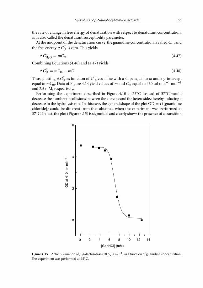
Hydrolysis of p-Nitrophenyl-β-D-Galactoside 55
the rate of change in free energy of denaturation with respect to denaturant concentration.m is also called the denaturant susceptibility parameter.
At the midpoint of the denaturation curve, the guanidine concentration is called Cm, andthe free energy �G0′
U is zero. This yields
�G◦′H2O = mCm (4.47)
Combining Equations (4.46) and (4.47) yields
�G0′U = mCm − mC (4.48)
Thus, plotting �G0′U as function of C gives a line with a slope equal to m and a y-intercept
equal to mCm. Data of Figure 4.14 yield values of m and Cm equal to 460 cal mol−1 mol−1
and 2.5 mM, respectively.Performing the experiment described in Figure 4.10 at 25◦C instead of 37◦C would
decrease the number of collisions between the enzyme and the heteroside, thereby inducing adecrease in the hydrolysis rate. In this case, the general shape of the plot OD = f ([guanidinechloride]) could be different from that obtained when the experiment was performed at37◦C. In fact, the plot (Figure 4.15) is sigmoidal and clearly shows the presence of a transition
OD
at 4
10 n
m m
in−1
6
0
2
4
0 2 4 6 8 10 12 14
[GdnHCI] (mM)
Figure 4.15 Activity variation of β-galactosidase (18.5μgml−1) as a function of guanidine concentration.The experiment was performed at 25◦C.

56 Principles and Applications of Fluorescence Spectroscopy
Figure 4.16 Variation of �G◦′ with guanidine chloride concentration at 25◦C.
point at 7 mM guanidine. Thus, lowering the temperature shows that there is at least oneintermediate structure between folded and unfolded structures of β-galactosidase. Plotting�G◦′ as a function of guanidine chloride concentration allows the values of m and Cm tobe determined, i.e., 535 cal mol−1 mol−1 and 7.8 mM, respectively (Figure 4.16). Resultsobtained with guanidine chloride show that β-galactosidase activity is dependent on theconcentration of the denaturing solvent and that the denaturation rate is temperature-dependent. Also, these experiments show that β-galactosidase unfolding would induce thepresence of intermediate states.
4.6.7 Effect of guanidine chloride on hydrolysis kinetics ofp-nitrophenyl-β-D-galactoside
Mix in a test tube 0.2 ml of 1 M guanidine with 1.8 ml of enzyme solution stock. The newstock solution is 0.1 M guanidine.
Prepare 11 test tubes with 0.5 ml of 10 mM heteroside and 1.5 ml of pH 7 buffer mixedtogether, and keep the test tubes at 37◦C for 5 min. Then, to each tube add 0.15 ml of themixture (enzyme–guanidine), mix and let the reaction continue at 37◦C. After 0, 1, 2, 3, 4,

Hydrolysis of p-Nitrophenyl-β-D-Galactoside 57
Figure 4.17 Activity of β-galactosidase with time in the presence of 7 mM guanidine chloride. Analysisof the exponential decrease as the sum of two exponentials yields decay times of 2.9 and 14.5 min.
5, 10, 15, 20, 25, and 30 min, add 3 ml of Na2CO3, mix, and measure the OD at 405 nm.Finally, plot the OD as a function of time and calculate the decay times of the curve.
What can you conclude about the denaturation process of β-galactosidase?
4.6.7.1 Results
Figure 4.17 displays β-galactosidase activity in the presence of 7 mM of guanidine chlorideas a function of time. Analysis of the decay curve yields two decay times equal to 2.9and 14.5 min. These times reveal mainly that the denaturation process of a protein doesnot occur in one simple step. The structure and dynamics of the protein should play animportant role in the accessibility of the guanidine chloride to the amino acids and so tothe unfolding process.
References
Bradford, M.M. (1976). A rapid and sensitive method for the quantitation of microgram quantititesof protein utilizing the principle of protein-dye binding. Analytical Biochemistry, 72, 248–254.

58 Principles and Applications of Fluorescence Spectroscopy
Carpita, N.C. and Gibeaut, D.M. (1993). Structural models of primary cell walls in flowering plants:consistency of molecular structure with the physical properties of the walls during growth. PlantJournal, 3, 1–30.
Murata, T., Hattori, T., Amarume, S., Koichi, A. and Usui, T. (2003). Kinetic studies onendo-beta-galactosidase by a novel colorimetric assay and synthesis of N -acetyllactosamine-repeating oligosaccharide beta-glycosides using its transglycosylation activity. European Journalof Biochemistry, 270, 3709–3719.
Stolle-Smits, T., Gerard Beekhuizen, J., Kok, M.T.C., Pijnenburg, M., Jan Derksen, K.R. and Voragen,A.G.J. (1999). Changes in cell wall polysaccharides of green bean pods during development. PlantPhysiology, 121, 363–372.
Talbott, L.D. and Ray, P.M. (1992). Molecular size and separability features of pea cell wallpolysaccharides: implications for models of primary structure. Plant Physiology, 98, 357–368.
http://www.mpbio.com/product_info.php?cPath=491_1_12&products_id=150039&depth=nested&keywords=beta%20galactosidase

Chapter 5Starch Hydrolysis by Amylase
Experiment conducted by Quanzeng Wang under the supervision of Professor Nam SunWang, Department of Chemical and Biomolecular Engineering, University of Maryland,College Park, MD 20742, USA.
5.1 Objectives
The objective is to study the various parameters that affect the kinetics of α-amylase-catalyzed hydrolysis of starch.
5.2 Introduction
Starchy substances constitute the major part of the human diet for most people in the world,as well as many other animals. They are synthesized naturally in a variety of plants. Examplesof plants with a high starch content include corn, potato, rice, sorghum, wheat, and cassava.It is no surprise that all of these are part of what we consume to derive carbohydrates.Similar to cellulose, starch molecules are glucose polymers linked together by α-1,4 andα-1,6 glucosidic bonds, as opposed to the β-1,4 glucosidic bonds for cellulose. In orderto make use of the carbon and energy stored in starch, the human digestive system, withthe help of the enzyme amylases, must first break down the polymer to smaller assimilablesugars, which are eventually converted to the individual basic glucose units.
Because of the existence of two types of linkages, α-1,4 and α-1,6, different structures arepossible for starch molecules. An unbranched, single-chain polymer of 500–2000 glucosesubunits with only α-1,4 glucosidic bonds is called amylose. On the other hand, the presenceof α-1,6 glucosidic linkages results in a branched glucose polymer called amylopectin.The degree of branching in amylopectin is approximately one per 25 glucose units inthe unbranched segments. Another closely related compound functioning as the glucosestorage in animal cells is called glycogen, which has one branching per 12 glucose units. Thedegree of branching and the side-chain length vary from source to source, but in generalthe more the chains are branched, the more the starch is soluble.
Starch is generally insoluble in water at room temperature. Because of this, starch in natureis stored in cells as small granules, which can be seen under a microscope. Starch granules arequite resistant to penetration by both water and hydrolytic enzymes due to the formationof hydrogen bonds within the same molecule and with other neighboring molecules.However, these inter- and intra-hydrogen bonds can become weak as the temperature of thesuspension is raised. When an aqueous suspension of starch is heated, the hydrogen bondsweaken, water is absorbed, and the starch granules swell. This process is commonly called

60 Principles and Applications of Fluorescence Spectroscopy
gelatinization because the solution formed has a gelatinous, highly viscous consistency. Thesame process has long been employed to thicken broth in food preparation.
Depending on the relative location of the bond under attack as counted from the end ofthe chain, the products of this digestive process are dextrin, maltotriose, maltose, glucose,etc. Dextrins are shorter, broken starch segments that form as the result of the randomhydrolysis of internal glucosidic bonds. A molecule of maltotriose is formed if the thirdbond from the end of a starch molecule is cleaved; a molecule of maltose is formed if thepoint of attack is the second bond; a molecule of glucose results if the bond being cleavedis the terminal one; and so on. The initial step in random depolymerization is the splittingof large chains into various smaller segments. The breakdown of large particles drasticallyreduces the viscosity of gelatinized starch solution, resulting in a process called liquefactionbecause of the thinning of the solution. The final stages of depolymerization are mainly theformation of mono-, di-, and tri-saccharides. This process is called saccharification, due tothe formation of saccharides.
Since a wide variety of organisms, including humans, can digest starch, α-amylase isobviously widely synthesized in nature, as opposed to cellulase. For example, human salivaand pancreatic secretion contain a large amount of α-amylase for starch digestion. Thespecificity of the bond attacked by α-amylases depends on the sources of the enzymes.Currently, two major classes of α-amylases are commercially produced through microbialfermentation. Based on the points of attack in the glucose polymer chain, they can be classi-fied into two categories, liquefying and saccharifying. Because the bacterial α-amylase to beused in this experiment randomly attacks only the α-1,4 bonds, it belongs to the liquefyingcategory. The hydrolysis reaction catalysed by this class of enzymes is usually carried out onlyto the extent that, for example, the starch is rendered soluble enough to allow easy removalfrom starch-sized fabrics in the textile industry. The paper industry also uses liquefyingamylases on the starch used in paper coating where breakage into the smallest glucosesubunits is actually undesirable (one cannot bind cellulose fibers together with sugar!)
On the other hand, the fungal α-amylase belongs to the saccharifying category andattacks the second linkage from the nonreducing terminals (i.e., the C4 end) of the straightsegment, resulting in the splitting off of two glucose units at a time. Of course, the productis a disaccharide called maltose. The bond breakage is thus more extensive in saccharifyingenzymes than in liquefying enzymes. The starch chains are literally chopped into smallbits and pieces. Finally, the amyloglucosidase (also called glucoamylase) component of anamylase preparation selectively attacks the last bond on the nonreducing terminals. The typeto be used in this experiment can act on both the α-1,4 and the α-1,6 glucosidic linkages ata relative rate of 1:20, resulting in the splitting off of simple glucose units into the solution.Fungal amylase and amyloglucosidase may be used together to convert starch to simplesugars. The practical applications of this type of enzyme mixture include the production ofcorn syrup and the conversion of cereal mashes to sugars in brewing.
Thus, it is important to specify the source of enzymes when the actions and kineticsof the enzymes are compared. In the present work, α-amylases from microbial originwill be employed. The effects of temperature, pH, substrate concentration, and inhibitorconcentration on the kinetics of amylase-catalysed reactions will be studied. Finally, it isimportant and interesting to know that the more accurate name for α-amylase is 1,4-α-d-glucan-glucanohydrolase (EC 3.2.1.1); for β-amylase, 1,4-α-d-glucanmaltohydrolase(EC 3.2.1.2); and for amyloglucosidase, exo-1,4-α-glucosidase or 1,4-α-d-glucanglucohydrolase (EC 3.2.1.3).

Starch Hydrolysis by Amylase 61
5.3 Materials
• α-Amylase (EC 3.2.1.1): Type VIII-A, from barley malt [9000-90-2], Sigma A-2771, lot124H0151. Prepare a 20 g l−1 solution
• Sigma’s definition: 1 unit liberates 1.0 mg of maltose from starch in 3 min at pH 6.9 at20◦C
• Purity: 1.1 units α-amylase per milligram of solid, 1.7 units β-amylase per milligram ofsolid at pH 4.8
• Starch: potato, soluble [9005-84-9], Sigma S-2630, lot 44H0156. Prepare a 20 g l−1
solution• Maltose: maltose, hydrate, Sigma M-5885, lot 37F0869• Glucose: d-(+)-glucose, Sigma G-7021, lot 76H0043• HCl stopping solution, 0.1N HCl• Iodine reagent stock solution (in aqueous solution). See Note 1• Iodine: 5 g l−1
• KI: 50 g l−1
• KH2PO4 (monobasic phosphate) (FW = 136.1)• K2HPO4 · 3H2O (dibasic phosphate) (FW = 228.23)• CaCl2 · 2H2O, 0.1 M solution• Reagents for the analysis of reducing sugars• Room temperature = 22.5◦C
5.4 Procedures and Experiments
5.4.1 Preparation of a 20 g l−1starch solution
Mix 20 g of soluble potato starch in approx. 50 ml of cold water. While stirring, add theslurry to approx. 900 ml of gently boiling water in a large beaker. Mix well and cool thegelatinized starch solution to room temperature. Add more water to bring the total volumeup to 1 l. Put a few drops of the starch solution on a glass plate. Add 1 drop of the iodinereagent; you should see that a deep blue color is developed. The blue color indicates thepresence of starch in the solution.
5.4.2 Calibration curve for starch concentration
Add 0.1 ml of sample to 1 ml of 0.1 N HCl, and then add 0.2 ml of the mixture to 2 mlof iodine solution. Finally, measure the absorbance with the spectrophotometer at 620 nm(note 2). The resulting data and plot of starch concentration as a function of absorbanceare shown in Table 5.1 and Figure 5.1, respectively.
5.4.2.1 Conclusion
The linear plot (Figure 5.1) indicates that the intensity of the blue color is directly relatedto starch concentration.

62 Principles and Applications of Fluorescence Spectroscopy
Table 5.1 Absorbance at 620 nm for different starchconcentrations
Starch Volume ofconcentration 10 g l−1 Volume of Absorbance at(g l−1) Starch (ml) water (ml) 620 nm
0 0 2 0.0031 0.2 1.8 0.0802 0.4 1.6 0.1673 0.6 1.4 0.2364 0.8 1.2 0.3225 1 1 0.3956 1.2 0.8 0.4707 1.4 0.6 0.5538 1.6 0.4 0.6189 1.8 0.2 0.697
10 2 0 0.784
Figure 5.1 Calibration plot of starch concentration followed by absorbance at 620 nm.

Starch Hydrolysis by Amylase 63
5.4.3 Calibration curve for sugar concentration
Add 1 ml of DNS reagent to 1 ml of maltose (or glucose) sample. Heat the mixture to100◦C for 10 min. Then, add 0.33 ml of a 40% potassium sodium tartrate. Cool to roomtemperature in a cold water bath, and measure the absorbance at 575 nm.
The results are displayed in Table 5.2 and Figure 5.2.
Table 5.2 Absorbance variation at 575 nm as a function of glucose and maltose
Volume ofMaltose 10 g l−1 Absorbance of Absorbance of(or glucose) maltose Volume of maltose at glucose atconcentration (g l−1) (or glucose) (ml) water (ml) 575 nm 575 nm
0 0 1 0.015 0.0201 0.1 0.9 0.540 0.5762 0.2 0.8 1.068 1.1663 0.3 0.7 1.534 1.7084 0.4 0.6 1.993 2.1965 0.5 0.5 2.322 2.461
Figure 5.2 Optical-density variation at 575 nm as a function of maltose (a) and glucose (b) concentration.

64 Principles and Applications of Fluorescence Spectroscopy
5.4.3.1 Conclusion
Both maltose and glucose can be reliably measured, albeit the color intensities are slightlydifferent.
5.4.4 Effect of pH
The experiment is carried out at room temperature (22.5◦C).
1 Prepare 0.25 M pH buffer solutions ranging from pH 0.5 to 9. (Note that phosphatebuffer is only good for pH = 4.5–9 due to the dissociation constant.) Before coming tothe lab, review how to make a pH buffer solution in a freshman chemistry textbook andcalculate the relative amounts of KH2PO4 (monobasic phosphate) and K2HPO4·3H2O(dibasic phosphate) needed to make these phosphate buffer solutions.
2 Add an equal volume of one of the above buffer solutions to 2.0 ml of the 20 g l−1 starchsolution prepared in step 1. The resulting solution should contain 10 g l−1 of starch ina buffered environment.
3 Add 0.2 ml of the barley amylase to 2 ml of the 10 g l−1 buffered starch solution, andkeep the reaction going for 3 min.
4 After 3 min, stop the enzymatic reaction by adding 0.1 ml of the reacted starch solutionto 1 ml of the HCl stopping solution (0.1 N).
5 Then, add 0.2 ml of the above mixture to 2 ml of iodine solution to develop the color.Shake and mix. The solution should turn deep blue if there is any residual, unconvertedstarch present in the solution. The solution is brown-red for partially degraded starchbut clear for totally degraded starch.
6 Measure the absorbance at 620 nm. For an absorbance value, the equivalent starchconcentration is calculated from Figure 5.1.
7 Carry out the same procedure for the other starch solutions buffered at different pHs.Use your time wisely; all the solutions can be handled simultaneously if you are familiarwith the procedure. Slightly stagger the sequential sample withdrawal so that there isenough time for sample preparation and handling.
0.2 mlsample soln
0.1 ml
2 mlstarch soln
1 ml0.1N HCI soln
2 mliodine soln
0.2 ml
OD at 620 mm
Experimental data are shown in Table 5.3, and the results are displayed in Table 5.3 andFigure 5.3. The actual pH in Table 5.3 corresponds to the pH of the measurement.
5.4.4.1 Notes
Water is added instead of amylase in control experiments. Our enzymatic activity definitionis: 1 unit of amylase hydrolyses 1.0 mg of starch in 3 min at pH 6.6 at 20◦C.

Table5.3
Dataformeasuring
theba
rley
amylaseactiv
ityon
starch
atdiffe
rent
pH
With
amylase
Volum
eof
Volum
eof
20gl−
1Absorba
nceat
Correspon
ding
starch
Starch
Specificactiv
ityActua
lpH
Volum
eof
HCl(μ
l)water
(μl)
starch
(ml)
620nm
conc
entration(g
l−1)
mass(m
g)(unitsmg−
1)
0.78
2000
(1M)
02
0.57
07.3
0.7
100.97
900(1
M)
1100
20.54
26.9
0.7
1.2
1.50
200(1
M)
1800
20.57
67.4
0.7
1.0
2.90
21(0.1
M)
1979
20.41
95.3
0.5
2.1
3.38
7(0.1
M)
1993
20.37
84.8
0.5
2.4
pHof
Volum
eof
Volum
eof
Volum
eof
20gl−
1Absorba
nceat
Starch
conc
entration
Starch
Specificactiv
ityActua
lpH
0.25
Mbu
ffer
0.25
Mbu
ffer(m
l)water
(ml)
starch
(ml)
620nm
(gl−
1)mass(m
g)(unitsmg−
1)
4.6
4.45
0.4
0.6
10.19
52.4
0.2
3.7
5.6
5.48
0.4
0.6
10.37
64.8
0.5
2.4
6.6
6.52
0.4
0.6
10.52
86.7
0.7
1.3
7.6
7.58
0.4
0.6
10.60
77.8
0.8
0.7
8.4
8.5
0.4
0.6
10.66
8.4
0.8
0.4
9.1
9.3
0.4
0.6
10.63
88.2
0.8
0.5

66 Principles and Applications of Fluorescence Spectroscopy
Figure 5.3 Amylase activity with pH.
The pHs of the blue solutions are adjusted with 0.1 and 1 M HCl. In the experimentalconditions described here, in 0.1 ml sample, the initial starch at the beginning of theexperiment is 0.91 mg, and the initial amylase is 0.18 mg.
5.4.4.2 Conclusion
For the enzyme employed (α-amylase from barley), the optimum pH is about 4.5. As thepH moves away from the optimum value in either direction, the enzyme activity decreases.Note that from our experience (data not shown), the optimum pH depends on the sourceof the enzyme.
5.4.5 Temperature effect
Note: the solution can be prepared together and then separated to aliquots of 2 ml.
1 Obtain hot water from either a faucet or a hot temperature bath. Adjust the temperaturesof the temporary water baths in 500 ml beakers so that they range from 30 to 90◦C inincrements of 10◦C.

Starch Hydrolysis by Amylase 67
2 Prepare the starch substrate by diluting the 20 g l−1 starch solution prepared in step 1with an equal volume of pH 7.0 phosphate buffer solution. This results in a workingstarch concentration of 10 g l−1. Add 2 ml of the starch solution to each of the test tubes.
3 Allow the temperature of each of the starch solutions to reach equilibrium with that ofthe water bath.
4 Add 0.1 ml of the barley amylase to 2 ml of the thermostatted 10 g l−1 buffered starchsolution.
5 Let the enzyme act for 3 min.6 Add 0.1 ml of the reacted starch solution to 1 ml of the HCl stopping solution (0.1 N)7 Add 0.2 ml of the above mixture to 2 ml of iodine solution to develop the color.8 Measure the absorbance at 620 nm.
Follow exactly the procedure outlined in step 4 (experiment at different pH). In 0.1 mlsample, we have an initial starch value of 0.95 mg and initial amylase of 0.10 mg.
Tables 5.4 and 5.5 Show, respectively, the experimental procedure and the results obtainedin the presence of amylase and of water (control experiment), and Figures 5.4 and 5.5 show
Table 5.4 Experimental procedure and results obtained for starch hydrolysis in the presence of amylaseat different temperatures and at pH 7
With amylase
pH of Volume of Volume of Starch Specific
Temperature 0.25 M 0.25 M Volume of 20 g l−1 Absorbance at concentration Starch activity
(◦C) buffer buffer (ml) water (ml) starch (ml) 620 nm (g l−1) mass (mg) (units mg−1)
30 6.52 0.4 0.6 1 0.551 7.0 0.7 2.5
40 6.52 0.4 0.6 1 0.429 5.5 0.5 4.0
50 6.52 0.4 0.6 1 0.078 0.9 0.1 8.6
60 6.52 0.4 0.6 1 0.040 0.4 0.0 9.1
70 6.52 0.4 0.6 1 0.464 5.6 0.6 3.9
80 6.52 0.4 0.6 1 0.666 8.5 0.9 1.0
90 6.52 0.4 0.6 1 0.673 8.6 0.9 0.9
Table 5.5 Experimental procedure and results obtained for starch hydrolysis in the presence of water atdifferent temperatures
With water
pH of Volume of Volume of Volume of Absorbance at Starch StarchTemperature 0.25 M 0.25 M water 20 g l−1 620 nm concentration mass(◦C) buffer buffer (ml) (ml) starch (ml) (water control) (g l−1) (mg)
30 6.52 0.4 0.6 1 0.629 8.0 0.840 6.52 0.4 0.6 1 0.638 8.2 0.850 6.52 0.4 0.6 1 0.662 8.5 0.860 6.52 0.4 0.6 1 0.646 8.3 0.870 6.52 0.4 0.6 1 0.625 8.0 0.880 6.52 0.4 0.6 1 0.697 8.9 0.990 6.52 0.4 0.6 1 0.664 8.5 0.8

68 Principles and Applications of Fluorescence Spectroscopy
Figure 5.4 Determination of the optimum temperature of amylase activity.
Figure 5.5 Starch concentration at different temperatures in the presence of amylase (b) and of water (a).

Starch Hydrolysis by Amylase 69
the specific activity and the corresponding starch concentration, respectively, at differenttemperatures.
5.4.5.1 Conclusion
For the enzyme employed, the highest conversion occurs at about 50◦C. As temperatureincreases, the intrinsic enzyme activity increases; however, enzyme deactivation alsobecomes significant. Note that, as in the optimum pH, the optimum temperature dependson the source of the enzyme.
5.4.6 Effect of heat treatment at 90◦C
Note: the solution can be prepared together and then separated to aliquots of 5 ml.
1 Put 0.4 ml of the amylase solution in each of 11 tubes, and then place the tubes into a90◦C water bath.
2 Take out the first test tube after a certain time (min) and quickly bring it to roomtemperature in a cold water bath. Remove the second test tube after x min, the thirdafter y min, and so on. Add 2 ml of 10 g l−1 buffered/nonbuffered starch at roomtemperature to each tube, and continue the enzymatic reaction for 3 min.
3 Add 0.1 ml of the reacted starch solution to 1 ml of the HCl stopping solution (0.1 N)4 Add 0.2 ml of the above mixture to 2 ml of iodine solution to develop the color, then
measure the absorbance at 620 nm.
Do not forget to follow exactly the procedure outlined in the experiment at different pH.In 0.1 ml sample, initial starch: 0.83 mg and initial amylase: 0.33 mg. [Ca2+] = 0.08 M. ThepH of 0.25 M buffer used is 6.52, which is the pH (6.5) of the experiment.
The experiment should be performed under three conditions: with buffer (Table 5.6),without buffer (only water is added) (Table 5.7), and in CaCl2 solution to investigate theheat stabilization of the enzymes in the presence of Ca2+ ions (Table 5.8).
Figures 5.6 and 5.7 show, respectively, amylase activity and starch concentration vs.heating time at 90◦C in the presence and absence of buffer.
Figures 5.8 and 5.9 show, respectively, amylase activity and starch concentration vs.heating time at 90◦C in the presence and absence of CaCl2.
Table 5.6 Specific activity data for amylase activity after heat treatment of buffered enzyme at 90◦C
Volume of Volume of Volume of Starch Starch SpecificHeat time 0.25 M water 20 g l−1 Absorbance concentration mass activity(min) buffer (ml) (ml) starch (ml) At 620 nm (g l−1) (mg) (units mg−1)
0.0 0.4 0.6 1 0.399 5.1 0.5 1.00.3 0.4 0.6 1 0.492 6.3 0.6 0.60.7 0.4 0.6 1 0.511 6.5 0.7 0.51.0 0.4 0.6 1 0.549 7.0 0.7 0.42.0 0.4 0.6 1 0.613 7.8 0.8 0.13.5 0.4 0.6 1 0.619 7.9 0.8 0.15.0 0.4 0.6 1 0.621 7.9 0.8 0.1

70 Principles and Applications of Fluorescence Spectroscopy
Table 5.7 Specific activity data of amylase activity after heat treatment of buffered enzyme at 90◦C
Volume of Volume of Volume of Starch Starch SpecificHeat time 0.25 M water 20 g l−1 Absorbance concentration mass activity(min) buffer (ml) (ml) starch (ml) at 620 nm (g l−1) (mg) (units mg−1)
0.0 0 1 1 0.401 5.1 0.5 1.00.3 0 1 1 0.489 6.2 0.6 0.60.7 0 1 1 0.517 6.6 0.7 0.51.0 0 1 1 0.58 7.4 0.7 0.32.0 0 1 1 0.587 7.5 0.8 0.23.5 0 1 1 0.592 7.6 0.8 0.25.0 0 1 1 0.598 7.6 0.8 0.2
Table 5.8 Specific activity data of amylase after heat treatment of enzyme at 90◦C in the absence ofbuffer and presence of CaCl2
Volume of Volume of Volume of Starch Starch SpecificHeat time 0.2 M water 20 g l−1 Absorbance concentration mass activity(min) CaCl2 (ml) starch (ml) at 620 nm (g l−1) (mg) (units mg−1)
0.0 0.2 0.8 1 0.41 5.2 0.5 0.90.3 0.2 0.8 1 0.495 6.3 0.6 0.60.7 0.2 0.8 1 0.545 7.0 0.7 0.41.0 0.2 0.8 1 0.606 7.8 0.8 0.22.0 0.2 0.8 1 0.629 8.0 0.8 0.13.5 0.2 0.8 1 0.648 8.3 0.8 0.05.0 0.2 0.8 1 0.651 8.3 0.0
5.4.6.1 Conclusion
The rate of deactivation is temperature-dependent. At 90◦C (which data are shown), thisenzyme becomes completely deactivated in ∼4 min.
5.4.7 Kinetics of starch hydrolysis
This experiment is performed under two conditions: in the absence and presence of 0.25 Mbuffer (pH 6.52).
In the absence of buffer, 1.2 ml of water is added to 1.2 ml of 20 g l−1 starch. Then, 0.1 mlof the barely enzyme is added to the 2.4 ml, 10 g l−1 starch solution.
In the presence of buffer, 2.4 ml of 0.25 M buffer is mixed with 3.6 ml of water and 6 mlof 20 g l−1 starch. Then, 0.5 ml of the barely enzyme is added to the 5 ml, 10 g l−1 starchsolution. Then, the procedure follows that described in the heat-treatment section. In thereaction mixture, the initial starch concentration is 9.6 mg ml−1, and the initial amylaseconcentration is 0.80 mg ml−1.

Starch Hydrolysis by Amylase 71
Figure 5.6 Specific activity of amylase as a function of heating time at 90◦C, in the presence (a) andabsence of buffer (b).
Figure 5.7 Starch concentration with heating time of amylase at 90◦C, in the presence (a) and absence(b) of buffer.

72 Principles and Applications of Fluorescence Spectroscopy
Figure 5.8 Amylase activity vs. heating time at 90◦C, in the presence (a) and absence (b) of CaCl2.
Figure 5.9 Starch concentration vs. heating time at 90◦C, in the presence (a) and absence (b) of CaCl2.
Starch Hydrolysis by Amylase 73
Table 5.9 Experimental data and results of starch hydrolysis withtime in the absence of buffer (pH 6.2 + 0.1)
Time (min) Absorbance at 620 nm Starch concentration (g l−1)
0 0.639 8.22 0.566 7.24 0.507 6.56 0.449 5.79 0.355 4,512 0.238 3.017 0.095 1.121 0.049 0.625 0.032 0.3
Table 5.10 Experimental data and results of starch hydrolysis with time in the presence of buffer(pH 6.4 + 0.1)
Starch Equivalent maltose Equivalent glucoseTime Absorbance concentration Absorbance concentration concentration(min) at 620 nm (g l−1) at 575 nm (g l−1) (g l−1)
0.1 0.629 8.0 0.008 2.2 1.22 0.588 7.5 0.008 2.2 1.24 0.508 6.5 0.008 2.2 1.26 0.441 5.6 0.008 2.2 1.29 0.363 4.6 0.008 2.2 1.212 0.256 3.2 0.008 2.2 1.217 0.115 1.4 0.01 2.8 1.621 0.114 1.4 0.011 3.0 1.825 0.112 1.4 0.011 3.0 1.8
The experimental data and results obtained are shown in Tables 5.9 and 5.10, andFigures 5.10 and 5.11.
5.4.8 Effect of inhibitor (CuCl2) on the amylase activity
The experiment is performed in the absence of buffer, since addition of CuCl2 to the mediumin the presence of buffer induces the formation of a precipitate. 0.5 ml of the barely enzymeis mixed to 0.6 ml of 0.2 M CuCl2, 0.6 ml water and 1.2 ml of 20 g l−1 starch. Then, theprocedure follows that described in the heat treatment section.
Table 5.11 shows the data obtained in the presence of 0.1 M CuCl2, and Figure 5.12 showsthe variation in starch concentration in the absence and presence of CuCl2.
5.4.9 Effect of amylase concentration
The experiment is carried out at 25◦C and at pH 6.52 (pH of the buffer). Add the barleyamylase to the starch solution and let the reaction continue for 3 min. Then, add 0.1 ml of the
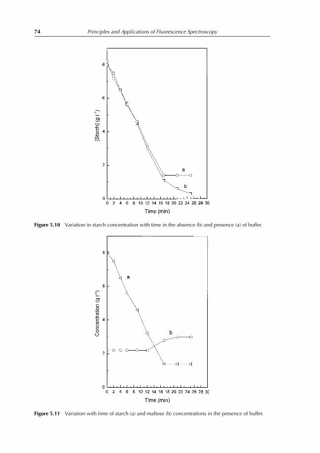
74 Principles and Applications of Fluorescence Spectroscopy
Figure 5.10 Variation in starch concentration with time in the absence (b) and presence (a) of buffer.
Figure 5.11 Variation with time of starch (a) and maltose (b) concentrations in the presence of buffer.

Starch Hydrolysis by Amylase 75
Table 5.11 Experimental data obtained for starch hydrolysis withamylase at room temperature in the presence of 0.1 M CuCl2
Time (min) Absorbance at 620 nm Starch concentration (g l−1)
1 0.620 7.92 0.602 7.74 0.583 7.56 0.566 7.29 0.535 6.812 0.511 6.518 0.474 6.021 0.461 5.925 0.452 5.8
Figure 5.12 Variation in starch concentration obtained in the absence (a) and presence (b) of CuCl2.
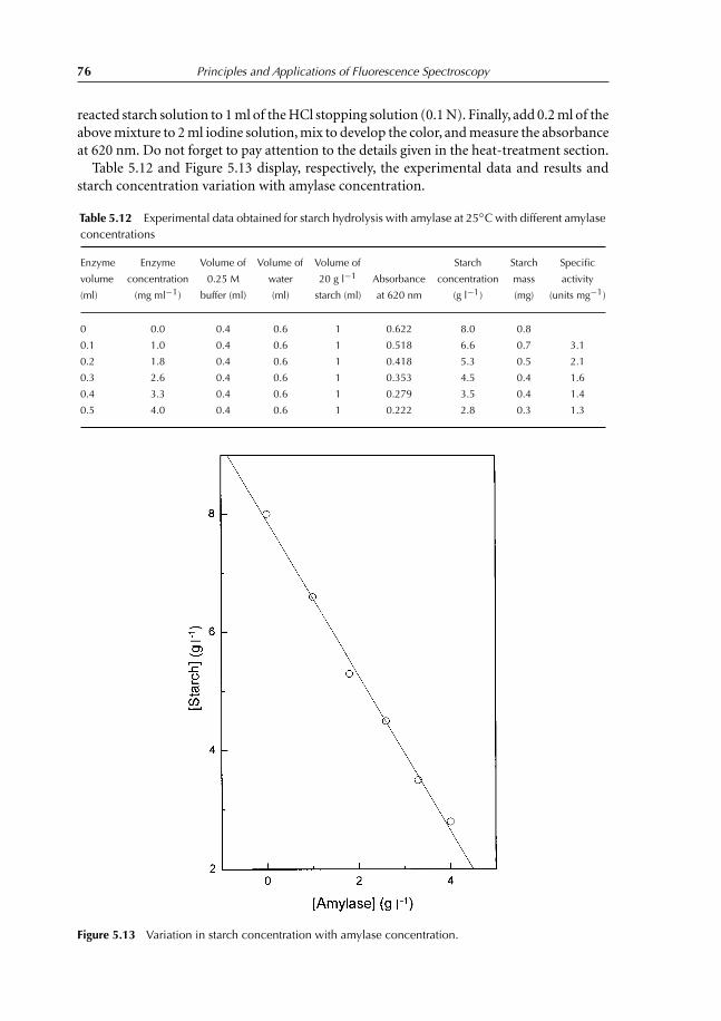
76 Principles and Applications of Fluorescence Spectroscopy
reacted starch solution to 1 ml of the HCl stopping solution (0.1 N). Finally, add 0.2 ml of theabove mixture to 2 ml iodine solution, mix to develop the color, and measure the absorbanceat 620 nm. Do not forget to pay attention to the details given in the heat-treatment section.
Table 5.12 and Figure 5.13 display, respectively, the experimental data and results andstarch concentration variation with amylase concentration.
Table 5.12 Experimental data obtained for starch hydrolysis with amylase at 25◦Cwith different amylaseconcentrations
Enzyme Enzyme Volume of Volume of Volume of Starch Starch Specific
volume concentration 0.25 M water 20 g l−1 Absorbance concentration mass activity
(ml) (mg ml−1) buffer (ml) (ml) starch (ml) at 620 nm (g l−1) (mg) (units mg−1)
0 0.0 0.4 0.6 1 0.622 8.0 0.8
0.1 1.0 0.4 0.6 1 0.518 6.6 0.7 3.1
0.2 1.8 0.4 0.6 1 0.418 5.3 0.5 2.1
0.3 2.6 0.4 0.6 1 0.353 4.5 0.4 1.6
0.4 3.3 0.4 0.6 1 0.279 3.5 0.4 1.4
0.5 4.0 0.4 0.6 1 0.222 2.8 0.3 1.3
Figure 5.13 Variation in starch concentration with amylase concentration.

Starch Hydrolysis by Amylase 77
5.4.9.1 Conclusion
Starch conversion in a fixed time relates linearly to the enzyme concentration.
5.4.10 Complement experiments that can be performed
5.4.10.1 Experiments with enzymes from different sources
The experiments described above can be repeated with enzymes from different sources,such as fungal amylase, amyloglucosidase, and a mixture of equivalent concentrations ofthree enzymes, bacterial amylase, fungal amylase, and amyloglucosidase.
5.4.10.2 Sequential enzymatic treatment (corn syrup production)
In making industrial sugars, e.g., corn syrup, large gelatinized starch molecules are firstchopped into smaller dextrins with the help of bacterial amylase. The liquefaction step isfollowed by saccharification with either fungal amylase or amyloglucosidase, depending onthe end use of the sugar. These sequential enzymatic treatment steps will be simulated inthis part of the experiment
Add 0.5 ml of the bacterial amylase solution to 50 ml of the 20 g l−1 nonbuffered starchsolution prepared in Step 1. Periodically place a few drops of the reaction mixture on a glassplate and add one drop of the iodine reagent. The color should finally turn red, indicatingthe total conversion of starch to dextrin. This liquefaction step should last for approximately10 min.
When the process of liquefaction is complete, adjust the pH of the starch solution to 4.7with 1 N HCl. Filter the starch solution if it is turbid. Separate the solution into two equalparts. To the first starch solution, add 0.5 ml of amyloglucosidase; to the second solution,add 0.5 ml of fungal amylase solution.
Measure the sugar concentrations periodically. Note that you need to use the appropriatecalibration curves because one is maltose, and the other is glucose. Also, do not forgetto reference your observation to the initial absorbance at the start of the saccharificationprocess so that the increase in the sugar concentration can be correctly measured. Thissaccharification step should last for about 30–60 min.
Taste the two sugar solutions and compare the sweetness. See Note 3.
5.4.10.3 Inhibition
Add hydrogen peroxide at a concentration of 0.5 g l−1 to the buffered starch solution atpH 7.0. If time permits, try hydrogen peroxide at a concentration of 1.0 g l−1.
5.4.11 Notes
1 Dilute the stock solution 1:100 to obtain a working solution. Other dilutions may beused, depending on the enzyme activity. Iodine does not dissolve well in water. Iodine(I2) alone or iodide (I−) alone does not color starch. It is the tri-iodide complex (I−3 ,
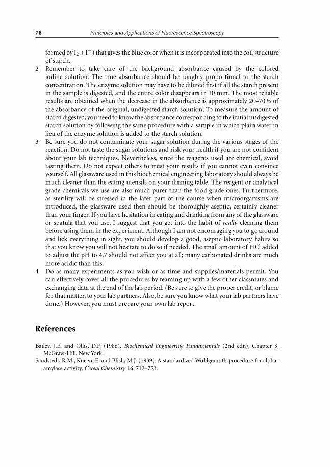
78 Principles and Applications of Fluorescence Spectroscopy
formed by I2 + I−) that gives the blue color when it is incorporated into the coil structureof starch.
2 Remember to take care of the background absorbance caused by the colorediodine solution. The true absorbance should be roughly proportional to the starchconcentration. The enzyme solution may have to be diluted first if all the starch presentin the sample is digested, and the entire color disappears in 10 min. The most reliableresults are obtained when the decrease in the absorbance is approximately 20–70% ofthe absorbance of the original, undigested starch solution. To measure the amount ofstarch digested, you need to know the absorbance corresponding to the initial undigestedstarch solution by following the same procedure with a sample in which plain water inlieu of the enzyme solution is added to the starch solution.
3 Be sure you do not contaminate your sugar solution during the various stages of thereaction. Do not taste the sugar solutions and risk your health if you are not confidentabout your lab techniques. Nevertheless, since the reagents used are chemical, avoidtasting them. Do not expect others to trust your results if you cannot even convinceyourself. All glassware used in this biochemical engineering laboratory should always bemuch cleaner than the eating utensils on your dinning table. The reagent or analyticalgrade chemicals we use are also much purer than the food grade ones. Furthermore,as sterility will be stressed in the later part of the course when microorganisms areintroduced, the glassware used then should be thoroughly aseptic, certainly cleanerthan your finger. If you have hesitation in eating and drinking from any of the glasswareor spatula that you use, I suggest that you get into the habit of really cleaning thembefore using them in the experiment. Although I am not encouraging you to go aroundand lick everything in sight, you should develop a good, aseptic laboratory habits sothat you know you will not hesitate to do so if needed. The small amount of HCl addedto adjust the pH to 4.7 should not affect you at all; many carbonated drinks are muchmore acidic than this.
4 Do as many experiments as you wish or as time and supplies/materials permit. Youcan effectively cover all the procedures by teaming up with a few other classmates andexchanging data at the end of the lab period. (Be sure to give the proper credit, or blamefor that matter, to your lab partners. Also, be sure you know what your lab partners havedone.) However, you must prepare your own lab report.
References
Bailey, J.E. and Ollis, D.F. (1986). Biochemical Engineering Fundamentals (2nd edn), Chapter 3,McGraw-Hill, New York.
Sandstedt, R.M., Kneen, E. and Blish, M.J. (1939). A standardized Wohlgemuth procedure for alpha-amylase activity. Cereal Chemistry 16, 712–723.
Chapter 6
Determination of the pK of a Dye
6.1 Definition of pK
Let us consider the following protonation reaction:
A + H+ ⇔ AH+ (6.1)
The protonation or association constant Ka of the complex is
Ka = [AH+]/[A][H+] (6.2)
[H+], [A], and [AH+] characterize the various concentrations:
log Ka = log([AH+]/[A]) − log[H+] (6.3)
log Ka = log([AH+]/[A]) + pH (6.4)
When A is protonated for 50%, that is, [AH+] = [A], we reach a pH called pK. Thus:
log Ka = log 1 + pK (6.5)
and
pK = log Ka (6.6)
6.2 Spectrophotometric Determination of pK
A pH-sensitive dye induces two different absorption spectra for the protonated (AH+) anddeprotonated (A) forms. This means that at low pHs, we observe an absorption spectrumof the protonated form only, while at a high pHs only the absorption spectrum of thedeprotonated form is recorded. However, this is not always true, since many dyes canabsorb in both forms, protonated and deprotonated. The absorption spectra maxima of thetwo forms are different. The protonated form displays an absorption spectrum with a peakthat is shifted toward short wavelengths in comparison with the absorption spectrum of thedeprotonated form of the dye.
Therefore, one method to determine the pK of a dye is to plot the peak position of theabsorption spectrum as a function of pH. A sigmoid curve is obtained; the pK is equal tothe pH at the inflection point.

80 Principles and Applications of Fluorescence Spectroscopy
A second method that allows determining the pK of a dye is to plot the optical densitiesas a function of the pH at two wavelengths λ1 and λ2, which are, respectively, the absorptionpeaks of the protonated and deprotonated forms. Thus, the acidic form of the dye absorbsstrongly at wavelength λ1, and the basic form absorbs strongly at λ2. At a low pH, we aregoing to monitor at λ1, mainly absorbance of the acidic form of the dye. Increasing the pHwill increase the concentration of the deprotonated form and decrease that of the protonatedform. Therefore, the optical density recorded at λ1 decreases when the pH increases. At alow pH and at λ2, we will record mainly the absorbance of the deprotonated form of thedye. However, since the deprotonated form is barely present at low pHs, a very weak opticaldensity is recorded. Increasing the pH induces the formation of deprotonated species, andso we shall observe an increase in the optical density at λ2. pK is equal to the pH where theconcentrations of the protonated and deprotonated forms of the dye are equal. In terms ofthe experiment, this corresponds to the pH where the absorbance of each form is half itsmaximum, i.e., at the inflection points of the two curves.
Also, a third method exists. This involves calculating the concentrations of both theprotonated and deprotonated forms at different pHs. The pK will correspond to the pHwhere the concentrations of both forms are equal. The derivation of the mathematicalequation used to determine the pK can be obtained as follows. The variation of the opticaldensity of the dye with the pH is sigmoidal. At low pHs in the presence of the protonatedform only, the optical density (OD(AH)) is
ODAH = εAHCAHl (6.7)
where ε·(AH), C(AH), and l are the molar extinction coefficient of the protonated form of thedye, its concentration, and the optical path length, respectively.
At high pHs, we observe the optical density of the deprotonated form only (OD(A)),which is
ODA = ε·ACAl (6.8)
where ε·(A), C(A), and l are the molar extinction coefficient of the deprotonated form of thedye, its concentration, and the optical path length, respectively.
When the dye is completely protonated or deprotonated, each of the concentrations C(AH)
and C(A) will be equal to the total concentration, C , of the dye. At an intermediate pH whereboth protonated and deprotonated forms are present, the optical density is
ODobs = ODAH + ODA = ε·AHCAHl + ε·ACAl (6.9)
where the total concentration C is
C = CAH + CA (6.10)
Equation (6.9) can also be written as
ODobs = ε·AH(C − CA)l + ε·ACAl (6.11)
= ε·AHCl − ε·AHCAl + ε·ACAl (6.12)
= ODAHC(Al(ε·A − ε·AH) (6.13)
Equation (6.13) can also be written as
ODobs = ODAH + XACl(ε·A − ε·AH) (6.14)

Determination of the pK of a Dye 81
where X(A) is the fraction of the protonated form of the dye.
ODobs = ODAH + XAClε·A − XAClε·AH
= ODAH + XAODA − XAODAH
= ODAH + XA[ODA − ODAH]ODobs − ODAH = XA[ODA − ODAH]
(6.15)
XA = ODobs − ODAH
ODA − ODAH(6.16)
XAH = 1 − XA = ODA − ODobs
ODA − ODAH(6.17)
One can replace [AH+] and [A] in Equation (6.4) with the fractions X(AH) and X(A)
expressed as optical densities (Equations (6.16) and (6.17)).
[AH+][A] = ODA − ODobs
ODA − ODAH:
ODobs − ODAH
ODA − ODAH= ODA − ODobs
ODobs − ODAH(6.18)
Combining Equations (6.18) and (6.4) yields
log Ka = logODA − ODobs
ODobs − ODAH+ pH (6.19)
pH = pK − logODA − ODobs
ODobs − ODAH(6.20)
pH = pK + logODobs − ODAH
ODA − ODobs(6.21)
Thus, plotting the pH as a function of
logODobs − ODAH
ODA − ODobs
will yield a straight line which intercepts the y-axis at a pH equal to the pK.
6.3 Determination of the pK of 4-Methyl-2-Nitrophenol
Methylnitrophenol such as p-nitrophenol is a weak acid similar in its ionization behaviorto phenol (Figure 6.1). It has the advantage of being colorless in its conjugate acid form andyellow in its conjugate base form (Figure 6.2).
6.3.1 Experimental procedure
Prepare a solution (2 ml) of methylnitrophenol in 10 mM Tris, pH 12. Add 10 μl of thissolution to 1 ml of 10 mM Tris buffer (pH 2–11).

82 Principles and Applications of Fluorescence Spectroscopy
OH
O2N
CH3
O2N
CH3
O−
+ H+
4-Methyl-2-nitrophenol, mNPH colorless 4-Methyl-2-nitrophenolate, mNP– yellow color
Figure 6.1 Ionization of 4-methyl-2-nitrophenol to 4-methyl-2-nitrophenolate.
Figure 6.2 Methylnitrophenol dissolved in 10mMTris buffer at pHs ranging from 2 (far left) to 12 (far right).The colorless protonated methylnitrophenol turns yellow when the pH increases. Reproduced in Colorplate 6.2.
1 After each addition, plot the absorption spectrum of the solution from 300 to500 nm. You will have 10 spectra characterizing absorption of methylnitrophenol atthe different pHs (2–11). What do you notice about the absorption peak position?Is there any correlation between the absorption peak position and the color of themethylnitrophenol solution? Do you observe an isobestic point? If yes, explain itsmeaning.

Determination of the pK of a Dye 83
2 Plot a graph showing the peak position of absorption spectrum of methylnitrophenolas a function of the pH. Determine the value of pK.
3 Plot a graph showing the optical density variation with pH at the peaks of the protonated(365 nm) and deprotonated (435 nm) forms of methylnitrophenol. What is the valueof pK?
4 Plot, at 350 nm, a graph of the pH as a function of
logODobs − ODAH
ODA − ODobs.
What is the value of pK? What other information you can gain from the graph? Choosetwo or three other wavelengths and plot the graph. Do you obtain the same pK for allthe graphs? Do you obtain the same pK with the three methods asked in 1, 2, and 3.
6.3.2 Solution
Color modification of the dye with the pH is accompanied by a shift in the absorptionpeak from short (365 nm) to higher wavelengths (435 nm). Figure 6.3 displays absorption
0.40
0.35
0.30
0.25
0.20
0.15
OD
0.10
0.05
0.00
−0.05300 350 400
Wavelength (nm)
450 500
a
b
Figure 6.3 Absorption spectra of methylnitrophenol inTris 10 mM, at pH 2 (a) and pH 11 (b). An isobesticpoint is observed at 385 nm.
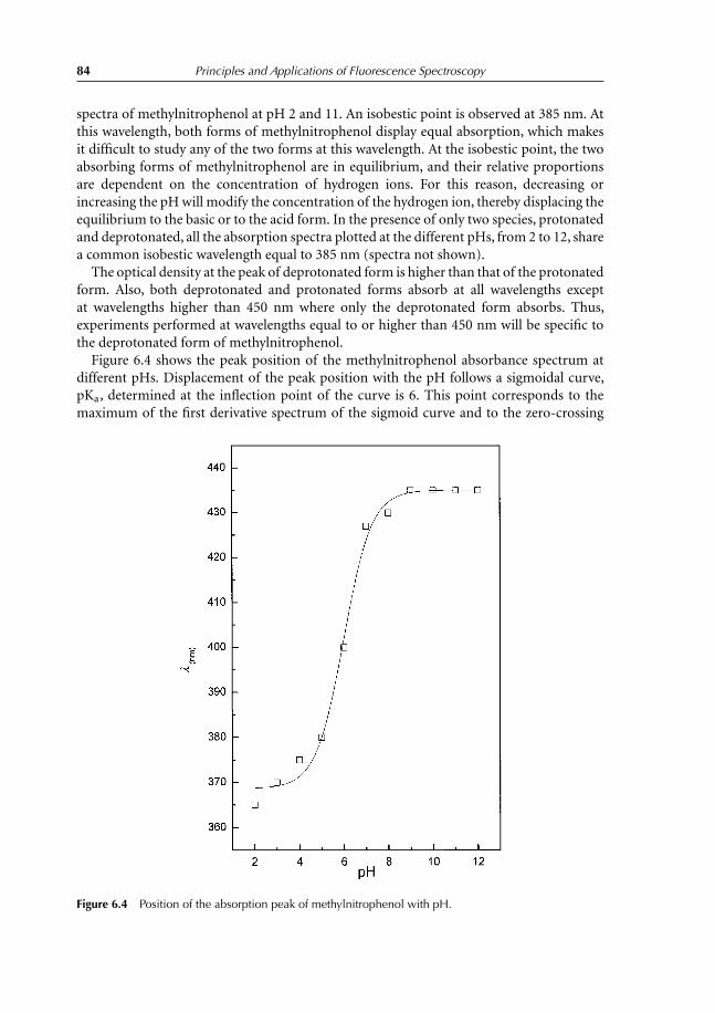
84 Principles and Applications of Fluorescence Spectroscopy
spectra of methylnitrophenol at pH 2 and 11. An isobestic point is observed at 385 nm. Atthis wavelength, both forms of methylnitrophenol display equal absorption, which makesit difficult to study any of the two forms at this wavelength. At the isobestic point, the twoabsorbing forms of methylnitrophenol are in equilibrium, and their relative proportionsare dependent on the concentration of hydrogen ions. For this reason, decreasing orincreasing the pH will modify the concentration of the hydrogen ion, thereby displacing theequilibrium to the basic or to the acid form. In the presence of only two species, protonatedand deprotonated, all the absorption spectra plotted at the different pHs, from 2 to 12, sharea common isobestic wavelength equal to 385 nm (spectra not shown).
The optical density at the peak of deprotonated form is higher than that of the protonatedform. Also, both deprotonated and protonated forms absorb at all wavelengths exceptat wavelengths higher than 450 nm where only the deprotonated form absorbs. Thus,experiments performed at wavelengths equal to or higher than 450 nm will be specific tothe deprotonated form of methylnitrophenol.
Figure 6.4 shows the peak position of the methylnitrophenol absorbance spectrum atdifferent pHs. Displacement of the peak position with the pH follows a sigmoidal curve,pKa, determined at the inflection point of the curve is 6. This point corresponds to themaximum of the first derivative spectrum of the sigmoid curve and to the zero-crossing
Figure 6.4 Position of the absorption peak of methylnitrophenol with pH.

Determination of the pK of a Dye 85
0.4
0.3
0.2
0.1
OD
0.0
2 4 6pH
8 10 12
b
a
Figure 6.5 Variation in optical density with pH at the peaks of protonated (365 nm) (curve a) anddeprotonated (435 nm) (curve b) forms of methylnitrophenol.
(the point where the signal crosses the x-axis going from either positive to negative or viceversa) in the second derivative.
Figure 6.5 shows the variation in optical density with pH at the peaks of the protonated(365 nm) and deprotonated (435 nm) forms of methylnitrophenol
The inflection point corresponding to pK is identical for both curves and is 6.2. Figure 6.6shows the graph of the pH as a function of
logODobs − ODAH
ODA − ODobs
at 350 nm.One can see that the pK is 6.2. This value is close to that (6) found for the pK with the two
previous methods (peak variation and optical density variation with the pH). Therefore,the three methods are coherent and can be used to determine the pK of a dye.
Figure 6.6 shows clearly that it is possible to apply Equation (6.21) at pH 4–7. In thispH range, we obtain a linear plot according to the equation used. At pHs lower than 4and higher than 7, Equation (6.21) can no longer be applied. Each dye has a specific pHapplication domain.

86 Principles and Applications of Fluorescence Spectroscopy
10
8
6
4
2
0−2 0 2
pH
Figure 6.6 Graph of the pH of methylnitrophenol as a function of log ODobs−ODAHODA−ODobs
at 350 nm. The pK
is found to be equal to 6.2.
10
8
6
4
2
0−1.0 −0.5 0.0 0.5 1.0 1.5 2.0
pH
Figure 6.7 Graph of the pH of methylnitrophenol as a function of log ODobs−ODAHODA−ODobs
at 410 nm. The pK
is found to be equal to 6.7.
Plotting the same graph at wavelengths equal to or higher than 400 nm yields a pK equalto 6.7. At these wavelengths, the pH domain in which Equation (6.21) can be applied isrestricted to two or three pH (6–8) (Figure 6.7). This result indicates that at wavelengthswhere absorption is dominated mainly by one species, the pK determined by this methodwould be more dependent on the form of the dye.

Determination of the pK of a Dye 87
Finally, pK determination is also dependent on the ionic strength of the solvent used. Inthe literature, the pKa of 4-methyl-2-nitrophenol is calculated to be equal to 7.11. Instructorsand students can refer to Aptula et al. (2002).
Reference
Aptula, A.O., Netzeva, T.I., Valkova, I.V. et al. (2002). Multivariate discrimination between modes oftoxic action of phenols. Quantitative Structure–Activity Relationships 21, 12–22.
Chapter 7Fluorescence Spectroscopy Principles
7.1 Jablonski Diagram or Diagram of Electronic Transitions
Absorption of light (photons) by a population of molecules induces electrons passage fromthe singlet ground electronic level S0 to an excited state Sn (n > l). An excited moleculewill return to the ground state S0 following two successive steps:
1 The molecule at Sn returns to the lowest excited state S1 by dissipating a part of itsenergy in the surrounding environment. This phenomenon is usually called internalconversion.
2 From the excited state S1, the molecule will reach the ground state S0 via differentcompetitive processes:• Emission of a photon (fluorescence) with a radiative rate constant kr.• Part of the absorbed energy is dissipated in the medium as heat. This type of energy
is nonradiative and occurs with a rate constant ki.• Excited molecules can release some of their energy to molecules located nearby. This
energy transfer occurs with a rate constant kq (collisional quenching), or with a rateconstant kt (energy transfer at distance).
• A transient passage occurs to the excited triplet state T1 of an energy lower thanS1 with a rate constant kisc (inter-system crossing). For each excited state S, thereis an excited state T of lower energy. The triplet state is an excited state and so isenergetically unstable.
Therefore, de-excitation of the molecule from the triplet state occurs via competitiveprocesses similar to those described for the de-excitation of the excited singlet state S1:
1 Emission of a photon with a rate constant kp. This phenomenon is calledphosphorescence.
2 Dissipation of nonradiative energy with a rate constant k ′i .
3 Transfer of energy to another molecule at distance (rate constant k ′t) or by collision (rate
constant k ′q) (Figure 7.1).

Fluorescence Spectroscopy Principles 89
S2
S1
S0
V0 V0
V5
T1
Heat
S0
V4
ki
Fluorescence
kisc
kq
kr
Fluorescence quenching
Phosphorescence
kp
Heat
Abs
orpt
ion
+h� 0
−h�
−h�′ki′
kg′Phosphorescencequenching
Internalconversion
Triplet Intersystem crossing
Figure 7.1 Jablonski (electronic transitions) diagram. Adapted from Jablonski, A. (1935). Zeitschrift furPhysik, 94, 38–64.
A chromophore that emits a photon is called a fluorophore. Many chromophores do notnecessarily fluoresce. In this case, energy absorbed is dissipated within the environmentas thermal energy, collisional energy as the result of permanent collisions with the solventmolecules, and also energy transfer to other molecules. For example, heme does absorblight, but it does not fluoresce. The absence of fluorescence is the result of total energytransfer from the porphyrin ring to iron.
The Jablonski diagram is also called the electronic transitions diagram, since electrons ofchromophores and/or fluorophores are responsible for the different described transitions.
The terminologies singlet and triplet state are the result of the spin quantum number s.Electron spinning around its own axis generates a local small magnet with a spin s. Singletand triplet states depend on the quantum number of spin of the electron (s). Accordingto the Pauli Exclusion Principle, two electrons within a defined orbital cannot have fourequal quantum numbers and so differ in spin number. Two spin numbers are attributed toan electron, + 1
2 and − 12 . Therefore, two electrons that belong to the same orbital will have
opposite spins.

90 Principles and Applications of Fluorescence Spectroscopy
↓ ↑
↑↓
↑↓ ↑↓
↑
↑↓
↑
Ground state
Mutiplicity = 1
Excited state
Mutiplicity = 1
Excited state
Mutiplicity = 3
Figure 7.2 Spin configurations of the singlet and triplet states.
A parameter called the multiplicity (M ) is defined as
M = |s1 + s2| + 1 (7.1)
When the spins are parallel, i.e., M = 1, we have a singlet state S. When the spins areanti-parallel, i.e., M = 3, we have a triplet state T (Figure 7.2).
Upon light absorption, electrons are under the effect of electric and magneticcomponents. The contributions of these two components in the transition process couldbe defined as
F = (eE) + (evH/c) (7.2)
where e, c , v , E , and H are, respectively, the electron charge, light velocity, speed of rotationof the electron on itself, and electric and magnetic components of the light wave. Theproducts (Ee) and (evH/c) are, respectively, the contributions of the electric and magneticfields to the absorption phenomenon.
The speed of electron rotation on itself is very weak compared to the light velocity,and so the magnetic contribution to absorption is negligible compared to the electriccontribution. Therefore, upon absorption, electronic transitions result from the interactionbetween electrons and electric field. For this reason, during absorption, a displaced electronpreserves the same spin orientation. This is why only the S0 → Sn transitions are allowed,and the S0 → Tn transitions are forbidden.
In the ground state, all molecules except oxygen are in the singlet form. Oxygen is inthe triplet state, and when excited, it reaches the singlet state. The singlet-excited state ofoxygen is destructive for cells having tumors. Such interactions are exploited for biomedicalapplications known as photodynamic therapy. Compounds such as porphyrins are localizedin target cells and tissues. Upon light activation, energy transfer occurs from porphyrins tooxygen molecules, thereby inducing a triplet → singlet transition within the oxygen state.Cells having tumor attract excited oxygen molecules and are then destroyed by these sameoxygen molecules.

Fluorescence Spectroscopy Principles 91
7.2 Fluorescence Spectral Properties
7.2.1 General features
Absorption allows a chromophore to reach an excited state, and so photon absorptioninduces excitation.
The absorption energy is higher than the emission energy. In fact, the total energyabsorbed by the molecule is released in the medium in different ways, such as photonemission. Thus, the energy of the emitted photons is lower than the energy of the absorbedphotons.
Many phenomena other than fluorescence emission contribute to fluorophore de-excitation. These other alternatives to fluorescence are radiationless loss, phosphorescence,photo-oxidation, and energy transfer. Thus, the weaker the competitive phenomena, thehigher the de-excitation via fluorescence.
Emission occurs from the excited state S1, independently of the excitation wavelength.Therefore, the emission energy would be independent of the excitation wavelength. Thefluorescence energy is higher than that of phosphorescence.
Absorption and fluorescence do not require any spin reorientation. However, intersystemcrossing and phosphorescence require a spin reorientation. Therefore, absorption andfluorescence are much faster than phosphorescence. Absorption occurs within a time equalto 10−15 s, and the fluorescence lifetime goes from 10−9 to 10−12 s. Phosphorescence is along transition that can last from milliseconds to seconds, minutes, or even hours.
The energy of electronic transition is equal to the energy difference between the startingenergy level and the final level. Therefore, the transition energy E (J mol−1) is:
E = hν = hc/λ (7.3)
where h is the Planck constant (h = 6.63×10⁻³⁴ J · s), ν is the light frequency (s−1 or Hertz,Hz), c is the light velocity, and λ is the wavelength (nm). Therefore, each transition occurswith a specific energy and so at a specific and single wavelength. However, as explained inthe first chapter, spectra are observed, and not single lines, as the results of the contributionof rotational and vibrational levels to absorption and de-excitation energy. The fluorescencespectrum generated shows a maximum corresponding to the emission transition.
The absorption spectrum occurs from the ground state. Therefore, it will characterize theelectronic distribution in this state. Fluorescence and phosphorescence occur from excitedstates, and so they are the mirrors of electronic distribution within the excited states, S forfluorescence and T for phosphorescence. Any modification of the electronic distributionin these states, such as in the presence of a charge transfer, will modify the correspondingspectrum. One such example is the reduction of cytochromes. The addition of an electronto the ground state, for example, modifies the electronic distribution within the moleculeaffecting the absorption spectrum.
Emission occurs from a population of n excited fluorophores with intensity I :
I = nE (7.4)
The emission lifetime is within the picosecond-to-nanosecond range. Thus, emission is avery fast process, and so in order to observe fluorescence emission, the fluorophore shouldbe excited continuously.

92 Principles and Applications of Fluorescence Spectroscopy
250 300 350 400 450 500 5500
2
4
6
8
10
12
14
16
18
20
22
Flu
ores
cenc
e in
tens
ity (
au)
Wavelength (nm)
ab
cd
Figure 7.3 Fluorescence excitation (a and b) and emission (c and d) spectra of the 7-amino-4-methylcoumarin–DEVD complex (spectra a and c) and of 7-amino-4-methylcoumarin, obtained afterautodissociation of the 7-amino-4-methylcoumarin–DEVD complex (spectra b and d). DEVD = Asp–Glu–Val–Asp. 7-Amino-4-methylcoumarin–DEVD complex: (a) λem = 470 nm and λgmax = 323 nm. (c) λex= 260 nm and λmax = 393 nm. 7-Amino-4-methylcoumarin: (b) λem = 440 nm and λmax = 350 nm. (d)λex = 300 nm and λmax = 438 nm.
Temperature variation induces modification of global and local motions of thefluorophore environment and of the fluorophore itself, modifying its fluorescence emissionfeature.
The intensity, position of the emission wavelength, and lifetime are some of theobservables that will characterize a fluorophore. Each fluorophore has its own fluorescenceproperties and observables. These properties are intrinsic to the fluorophore and aremodified with the environment. A fluorescence spectrum is the plot of the fluorescenceintensity as a function of wavelength (Figure 7.3).
Since we have to excite the sample and record the emitted intensity at differentwavelengths, the layout of a fluorometer consists of an excitation source (a lamp or a laser),an excitation monochromator or a filter (if a lamp is used as the source of excitation), acuvette holder into which we can put the sample, an emission monochromator or a filter

Fluorescence Spectroscopy Principles 93
Lamp
Beamsplitter
Excitationmonochromator
Polarizer
PMT
PMT
ShutterSample compartment
Lase
r
PMTShutter
Shutter
Emissionmonochromator
Polarizer
Polarizer
Shutter
Lightmodulator 1
11
4
5
12
6
10
S
R9
98
2
Figure 7.4 Layout of a spectrofluorometer. Courtesy of ISS Instruments.
(if we do not want to record the whole spectrum but just the fluorescence intensity), aphoton detector, and a recorder (Figure 7.4).
When we want to record the fluorescence emission spectrum, the excitation wavelengthis kept fixed, and the emission monochromator is run (Figures 7.3c and d). The excitationspectrum is obtained by running the excitation monochromator at a fixed emissionwavelength (Figures 7.3a and b).
7.2.2 Stokes shift
The energy absorbed by a fluorophore is more important than the energy of an emittedphoton. Referring to Equation (7.3), the absorption energy is
Ea = hc/λa (7.5)
and emission energy is
Eem = hc/λem (7.6)
Since
Eem < Ea (7.7)

94 Principles and Applications of Fluorescence Spectroscopy
We have
λem > λa (7.8)
λa and λem are absorption and emission spectra peaks.Thus, the emission spectrum has its maximum shifted to longer wavelengths compared
to the maximum of absorption spectrum (Figure 7.3). Sir George Stokes observed this shiftfor the first time in 1852 and since this time it is called the Stokes shift.
When absorption and/or the emission spectra of a fluorophore possess two or morebands, the Stokes shift is equal to the difference that separates the two most intense bandsof the two spectra.
7.2.3 Relationship between the emission spectrum andexcitation wavelength
Emission occurs from the excited state S1, and so is in principle independent from theexcitation wavelength.
Since not all the molecules present at the excited states will participate in the fluorescenceprocess, a quantum yield F exists:
F = IF
IA(7.9)
F < 1, since
IA = I0 − IF (7.10)
and
IT = I010−εcl = I0e−2.3εcl (7.11)
IA = I0 − I0e−2.3εcl = I0(1 − e−2.3εcl) (7.12)
At very low optical densities (�0.05), Equation (7.12) can be written as
I0(l − (l − 2.3ε(λ)cl)) = 2.3I0ε(λ)cl (7.13)
Thus,
IF(λ) = 2.3I0ε(λ)clF (7.14)
Equation (7.14) describes the relationship that exists between fluorescence intensity ata precise emission wavelength and intensity of incident light (I0), fluorophore quantumyield, and its optical density at the excitation wavelength.
I0 is the intensity of the incident beam that will excite the sample. Thus, excitation with alaser will allow yield a better fluorescence intensity than if a lamp were used for excitation.The fluorescence intensity is proportional to the quantum yield, i.e., a high quantum yieldleads automatically to a high fluorescence intensity.
The fluorescence intensity is proportional to the optical density. This means that it isproportional to εc and l . Since ε. is wavelength-dependent, the fluorescence intensity is alsowavelength-dependent.

Fluorescence Spectroscopy Principles 95
7.2.4 Inner filter effect
The fluorescence intensity is linearly proportional to the optical density (Equation (7.14)).However, let us take a usual fluorometer where the emission beam is recordedperpendicularly to the excitation beam. In general, emission is detected at the cuvettecenter. Thus, the incident beam will go through half the cuvette path length before emissionrecording. Also, the emission beam induced at the center of the cuvette should go throughhalf of the cuvette path length before being detected. Therefore, the recorded emissionintensity will be underestimated as the result of the optical density at both excitation andemission wavelengths. This auto-absorption by the solution is called the inner filter effect.It can modify the whole fluorescence spectrum inducing a shift in the emission maximumand a decrease in the fluorescence intensities.
The fluorescence intensity for the inner filter effect can be corrected using Equation (7.15)(Lakowicz, 1999; Albani, 2004):
Fcorr = Frec ∗ 10[OD(em)+OD(ex)]/2 (7.15)
7.2.5 Fluorescence excitation spectrum
The fluorescence excitation spectrum characterizes the electron distribution of the moleculein the ground state. Excitation is, in principle and for a pure molecule, equivalent toabsorption. The fluorescence excitation spectrum is obtained by fixing the emissionwavelength and by running the excitation monochromator (Figure 7.3).
The excitation spectrum is technically perturbed by two problems: the light intensity ofthe excitation lamp, which varies with the wavelength, and the intensity upon detection,which is also wavelength-dependent. Corrections can be performed using rhodamine B,dissolved in glycerol, as reference. In fact, radiation from rhodamine is proportional tothe excitation intensity independently of the excitation wavelengths. Therefore, excitationof rhodamine will yield a fluorescence excitation spectrum that characterizes excitationlamp spectrum. In order to obtain the real fluorescence excitation spectrum of thestudied fluorophore, the recorded excitation spectrum will be divided by the excitationspectrum obtained from rhodamine. This procedure is done automatically within thefluorometer.
In general, when one wants to determine if global and/or local structural modificationshave occurred within a protein, circular dichroism experiments are performed. Also, one canrecord the fluorescence excitation spectrum of the protein. If perturbations occur withinthe protein, one should observe excitation spectra that differ from one state to another. Oneshould not forget to correct the recorded spectra for the inner filter effect.
7.2.6 Mirror–image rule
The emission spectrum of a fluorophore is the image of its absorption spectrum whenthe probability of S1 → S0 transition is identical to that of S0 → S1 transition. If,however, excitation of the fluorophore leads to an S0 → Sn transition, with n > 1, internalrelaxation will occur so that molecules reach the first excited singlet state before emission.

96 Principles and Applications of Fluorescence Spectroscopy
This will induce an emission transition different from the absorption one. The mirror–image relationship is generally observed when the interaction of the fluorophore excitedstate with the solvent is weak.
7.2.7 Fluorescence lifetime
7.2.7.1 Definition of fluorescence lifetime
After excitation, molecules remain in the excited state for a short time before returning to theground state. The excited-state lifetime is equal to the mean time during which moleculesremain in the excited state. This time is considered as the fluorescence lifetime. This timeranges from the nanoseconds (10−9 s) to picoseconds (10−12 s).
The fluorescence lifetime τf is:
τf = 1/k = 1/(kr + kisc + ki) (7.16)
The mathematical definition of fluorescence lifetime arises from the fact that nonradiativeand radiative processes participate in the fluorophore deexcitation.
The radiative lifetime τr is l/kr. It is the real emission lifetime of a photon that shouldbe measured independently of the other processes that deactivate the molecule. However,since these processes occur in parallel to the radiative process, it appears impossible toeliminate them during radiative lifetime measurements. Therefore, we will measure a timecharacteristic of all deexcitation processes. This time is called the fluorescence lifetime andis lower than the radiative lifetime. A fluorophore can have one or several fluorescencelifetimes; in this case, we can determine the fractional contribution of each lifetime andcalculate the mean fluorescence lifetime τ0 or 〈τ 〉:
τ0 =∑
fiτi (7.17)
and
fi = βiτi
/ ∑βiτi (7.18)
where βi is the pre-exponential term, τi is the fluorescence lifetime, and fi is the fractionalintensity.
A fluorophore can have one or several fluorescence lifetimes, depending on severalfactors:
1 A ground-state heterogeneity resulting from the presence of equilibrium betweendifferent conformers. Each conformer presents a specific fluorescence lifetime.
2 Different nonrelaxing states of the Trp emission. These relaxed states may arise fromone single Trp residue.
3 Internal protein motion.4 The presence in the studied macromolecule, for example a protein, of two or several
tryptophans each having different microenvironments and so different emissions.
The nature of the environment and of its interaction with the fluorophore can affect all thefluorescence parameters.

Fluorescence Spectroscopy Principles 97
Also, it is important to mention that in many cases, fluorescence lifetimes are dependenton the structure of the fluorophore itself (Albani, 2007).
In general, fluorescence intensity decreases exponentially with time. Let us consider anN0 fluorophores population having reached the excited state. The velocity of decrease inthis population with time t is
−dN (t )
dt= (kr + k ′)N (t ) (7.19)
where kr is the radiative rate constant, k ′ the sum of rate constant of all other competingprocesses, and N (t ) the population at the excited state at time t .
dN (t )
N (t )= −(kr + k ′)dt (7.20)
log N = −(kr + k ′)t + constant (7.21)
At t = 0, N = N0, and log N = log N0
log N = −(kr + k ′)t + log N0 (7.22)
log N/N0 = −(kr + k ′)t (7.23)
N/N0 = e−(kr+k ′)t (7.24)
N = N0e−(kr+k ′)t (7.25)
τ = 1/(kr + k ′) (7.26)
N = N0e−t/τ (7.27)
When t = τ :
N = N0e−1 = N0/e (7.28)
Thus, we can define the fluorescence lifetime as the time required for the excited-statepopulation to be reduced by 1/e of its initial population, immediately after excitation.
7.2.7.2 Fluorescence lifetime measurement
Three techniques are actually available for measuring the fluorescence lifetime: Strobe,Time Correlated Single Photon Counting (TCSPC), and multifrequency and cross-correlation spectroscopy. Strobe and TCSPC are based on measurement in the time domain,while multifrequency and cross-correlation spectroscopy measure fluorescence lifetimes inthe frequency domain. The time domain allows direct observation of fluorescence decay,while the frequency domain is a more indirect approach in which the information regardingthe fluorescence decay is implicit.
In the time-correlated single-photon counting (TCSPC) technique, the sample is excitedwith a pulsed light source. The light source, optics, and detector are adjusted so that, for agiven sample, no more than one photon is detected. When the source is pulsed, a timer isstarted. When a photon reaches the detector, the time is measured. Over the course of the

98 Principles and Applications of Fluorescence Spectroscopy
0
2000
4000
6000
8000
10000
12000
1 2 3 4 5 6 7 8 9 10 11 12 13 14 15 16 17 18 19 20 21 22 23 24 25 26 27 28 29 30 31 32 33 34 35 36
Time, channels
Ph
oto
n c
ou
nts
MCA
S
CFDSYNC
IBH 5000 U
TBX-04
NanoLED
Statisticalsingle-photon
events
Periodic pulses
Cumulativehistogram
TACV
TAC rate 1MHzCoaxial delay 50 NsSync delay 20 ns
Figure 7.5 Time-correlated single-photon counting instrument principle. Courtesy of Jobin Yvon.
experiment, the fluorescence decay curve is constructed by measuring the “photon events,”or accumulated counts, vs. time (Figure 7.5) (Badea and Brand 1979).
In the strobe or pulse sampling technique, the sample is excited with a pulsed light source.The intensity of the fluorescence emission is measured in a very narrow time window oneach pulse and saved on the computer. The time window is moved after each pulse. Whendata have been sampled over the appropriate range of time, a decay curve of emissionintensity vs. time can be constructed.
The name “strobe technique” comes about because the photomultiplier PMT is gated –or strobed – by a voltage pulse that is synchronized with the pulsed light source. The strobehas the effect of “turning on” the PMT and measuring the emission intensity over a veryshort time window (Figure 7.6) (Bennett 1960; James et al. 1992).
In frequency-domain instruments, the sample is excited by a light source whose intensityis sinusoidally modulated (w). Emitted light will also be sinusoidally modulated at the samefrequency of the excited light but will be delayed by a phase angle, φ, due to the finitepersistence of the excited state. The phase angle, φ, is equal to (wθ), where θ is thephase delay time. The intensity of emitted light is lower than that of excitation light. Thefluorescence lifetime of the sample can be calculated from the phase delay and/or from lightdemodulation. A long fluorescence lifetime yields a highly delayed emission and a largephase shift between excitation and emission lights (Figure 7.7) (Spencer 1970).
A glycogen solution placed in the emission compartment will scatter light and is used asreference (τf = 0) to determine the phase delay and fluorescence demodulation. For eachmeasurement, the reference intensity is adjusted so that it is equivalent to the intensityof the fluorescence signal of the sample. Phases and modulations of the fluorescenceand scattered light are obtained relative to the reference photomultiplier or instrumental

Fluorescence Spectroscopy Principles 99
Time (�s)
Pho
ton
coun
ts
Figure 7.6 Schematic profile of the fluorescence lifetime measured by the Strobe method. Courtesy ofJobin Yvon.
1.0
(a)
(b)
0
Inte
nsity
30 MHz� = 9 ns
� = (ns)
� = 59.50
b
a A
0 20 40
Time (ns)
60
80 30 MHz
10 MHz60
40� (
°)
20
00 10 20 30 40
mL= __
B
ba
m = 0.5
= ___B/Ab/a
± 2°
= ± 0.35= ± 2.8 ns
Phase angleφ = tan-1 wT
Modulation
M = ____B /Ab /a
Figure 7.7 Determination of fluorescence lifetime from intensity modulation (a) and phase angle (b).

100 Principles and Applications of Fluorescence Spectroscopy
FFT:Fastfouriertransform
Spectracq
MHz
M
φ
R928PPMTSlave Rf+Δf
Master Rf
Amp450W
cw xenon
Pockels cell
Filter
Safe place
Sample turret
Am
p
Δf = Cross-correlation frequency
Figure 7.8 Multifrequency cross-correlation fluorometer. Courtesy of Jobin Yvon.
(internal) reference signal. In fact, two identical detection electronic systems are used toanalyze the outputs of the reference and sample photomultipliers. Each channel consists ofan alternative and continuous currents (AC and DC, respectively).
m = (AC/DC)EM/(AC/DC)EX = (B/A)/(b/a) (7.29)
where “EM” and “EX” refer to fluorescence and scattered light. Lifetimes can be obtainedby the phase method, denoted by τP, or by modulation, denoted by τM.
A mono-exponential decrease in fluorescence (one lifetime) yields τP = τM. A multi-exponential decrease gives τP < τM.
Multifrequency is achieved by using frequency modulators. The modulator currently usedis an electro-optic modulator that is crossed transversely by an electric current (Pockels cell)(Figure 7.8). In the phase detection system, high-frequency signals are used. In the cross-correlation technique, the high-frequency signals are converted to low-frequency signals.Excitation light is first modulated and then sent to the cell compartment equipped witha revolving turret so that it can excite the studied sample, then the reference, which is afluorophore of known fluorescence lifetime. This fluorophore replaces glycogen solution.
A part of the excitation light is sent toward a reference photomultiplier so that the intensityand phase of the excitation signal can be recorded. A frequency synthesizer connected tothe Pockels cell gives the desired frequency. Rather than to apply a continuous currenton the detection and reference photomultipliers, the two photomultipliers are submittedto a sinusoidal electric current R(t ) of frequency (w + �w) as close as possible to thefrequency w of the fluorescence light. �w is the cross-correlation frequency. The signalrecorded by the detection photomultiplier is thus the product of the emitted light F(t )and of R(t ). Therefore, the resulting signal evolves with a weak frequency �w possessingall information “contained” in the fluorescent light. One measures the evolution of thevalue 〈R(t ) ∗ F(t )〉 of the current delivered by the photomultiplier. This method, called

Fluorescence Spectroscopy Principles 101
cross-correlation, compares the excitation and emission signals. This double procedureconsiderably increases the signal-to-noise ratio.
For more details on the three different techniques, readers can refer to the followingreferences: Lakowicz (1999), Valeur (2002), and Albani (2004).
7.2.8 Fluorescence quantum yield
Molecules in the fundamental state absorb light with an intensity equal to I and reach anexcited state Sn . Then, different competitive processes, including fluorescence, will competewith each other to de-excite the molecule. The rate constant (k) of the excited state is thesum of the kinetic constants of the competitive processes:
k = kr + kisc + ki (7.30)
The fluorescence quantum yield F is the number of photons emitted by the radiative wayover that absorbed by the molecule:
F = emitted photons
absorbed photons= kr
kr + ki + kisc(7.31)
The fluorescence quantum yield of a molecule is obtained by comparing the fluorescenceintensity of the molecule with that of a reference molecule with a known quantum yield:
2 = OD1 ∗ �F2
OD2 ∗ �F11 (7.32)
where F2 is the fluorescence intensity of the molecule of unknown quantum yield 2, andF1 is the fluorescence intensity of the reference with quantum yield 1.
Therefore, in order to determine fluorophore quantum yield, one needs to measure theoptical densities of the fluorophore and of the reference at the excitation wavelength, and tocalculate for each of them the sum of their fluorescence intensities along their fluorescenceemission spectra.
In proteins, the quantum yield from the dominant fluorescent amino acid is calculated.For example, in a protein in which Trp residues are the main emitters, the quantum yieldis determined by comparison with a solution of free L-Trp (F = 0.14 at 20◦C and atλex = 295 nm). Also, quinine sulfate dissolved in 0.1 M sulfuric acid is commonly used as areference or standard molecule. Its quantum yield is 0.55 with an absorption and emissionmaxima at 340 and 445 nm, respectively.
Finally, one should remember that the standard and the molecule to be analyzed shouldbe studied under the same conditions of temperature and solvent viscosity. Also, it is alwaysbetter to work at low optical densities in order to avoid corrections for the inner filter effect.
In a multitryptophan protein, the fluorescence quantum yield of tryptophans can beadditive or not. In the first case, there is no interference between Trp residues. In the secondcase, energy transfer between tryptophan residues can influence the quantum yield of eachof them.
In order to measure quantum yields of an extrinsic fluorophore bound to a proteinand which emits at longer wavelengths than in the UV, standards such as 3,3′-diethylthiacarbocyanine iodide (DTC) in methanol (F = 0.048) and rhodamine 101

102 Principles and Applications of Fluorescence Spectroscopy
Table 7.1 Fluorescence observables of tryprophanin solvents of different pHs
F λmax (nm) τ0 (ns)
Basic 0.41 365 9Neutral 0.14 351 3.1Acid 0.04 344 0.7
in ethanol (F = 0.92) or any other dyes can be used. Quantum yield is calculated accordingto Equation (7.33):
S
R= AS
AR× ODR
ODS× n2
S
n2R
(7.33)
where, S and R are the fluorescence quantum yields of the sample and reference,respectively. AS and AR are areas under the fluorescence spectra of the sample and thereference, respectively; (OD)S and (OD)R are the respective optical densities of the sampleand the reference solution at the excitation wavelength; and nS and nR are the values of therefractive index for the respective solvents used for the sample and reference (Barik et al.2003).
Table 7.1 shows the fluorescence lifetime, quantum yield, and position of the emissionmaximum of tryptophan in basic, neutral, and acidic solvents. One can see that the threeparameters are not the same in the three media. The different types of protonation explainthis variation.
7.2.9 Fluorescence and light diffusion
There are two types of light diffusion: Rayleigh and Raman. Energies of diffused and excitedphotons are equal. Thus, Rayleigh diffusion and excitation occurs at the same wavelengths.
Usually, one should not start recording the emission spectrum before or at the excitationwavelength in order to avoid recording Rayleigh diffusion. Raman diffusion is observedat a wavelength higher than the excitation wavelength. Diffused photons have a quantumenergy lower than that of the excitation photons. Therefore, the intensity of the Raman peakis lower than that of the Rayleigh peak. Raman diffusion can perturb emission spectrum,and so one should substract Raman from the emission spectrum. In general, the higher thefluorescence intensity, the lower the Raman peak (Figure 7.9). In an aqueous medium, theO−−H bonds are responsible for the Raman spectrum. The position of the Raman peak isdependent on the excitation wavelength. It is possible to calculate the position of the Ramanpeak in an aqueous medium using the following equation:
1/λram = 1/λex − 0.00034 (7.34)
The wavelengths are in nanometers.
7.3 Fluorophore Structures and Properties
Fluorophores, small molecules that can be part of a molecule (intrinsic fluorophores) oradded to it (extrinsic fluorophores), can be found in different cells, and so they can be

Fluorescence Spectroscopy Principles 103
(a) (b)
(c)
Figure 7.9 (a) Fluorescence emission spectrum of α1-acid glycoprotein before (a) and after (c) Rayleighand Raman substraction of the buffer (spectrum b). Raman peak makes up 3.75% of the peak in spectrum(a). λex = 295 nm. (b) Fluorescence emission spectrum of α1-acid glycoprotein before (a) and after (c)Rayleigh and Raman substraction of the buffer (spectrum b). Raman peak makes up 9.34% of the peak inspectrum (a). λex = 300 nm. (c) Fluorescence emission spectrum of α1-acid glycoprotein before (a) andafter (c) Raman substraction of the buffer (spectrum b). The Raman peak makes up 25% of the peak inspectrum (a). λex = 305 nm.

104 Principles and Applications of Fluorescence Spectroscopy
1.0
0.5
0
240 280 320 360
Wavelength (nm)
400 440
303 nmTry
348 nmTrp
282 nmPhe
Flu
ores
cenc
e in
tens
ity
Figure 7.10 Fluorescence emission spectra of aromatic amino acids.
used as natural indicators to study the structure, dynamics, and metabolism of living cells.Their fluorescence properties are dependent on their structure and on the surroundingenvironment. Each fluorophore has its own specific fluorescence properties. Intrinsicfluorophores are aromatic amino acids and cofactors. Extrinsic fluorophores are those whichcan be linked covalently or not to macromolecules such as peptides, proteins, membranes,or DNA.
7.3.1 Aromatic amino acids
In proteins, tryptophan, tyrosine, and phenylalanine are responsible for the absorption andfluorescence of proteins in the UV (Figures 1.2 and 7.10).
Tryptophan fluorescence is very sensitive to the local environment. In an environmentwith a low polarity, tryptophan emits at a maximum of 320 nm. The peak position shifts to355 nm in the presence of a polar environment. The loss of the protein tertiary structure(complete denaturation) induces a shift in tryptophan fluorescence to 355 nm.
Also, upon binding of a ligand to a protein, Trp observables (intensity, polarization, andlifetime) can be altered, and so one can follow this binding with Trp fluorescence. In proteins,tryptophan fluorescence dominates. Zero or weak tyrosine and phenylalanine fluorescenceresults from energy transfer to tryptophan and/or neighboring amino acids.
Burstein et al. (1973) classified tryptophan in proteins into three categories, accordingto the position of their fluorescence maximum (λmax) and the bandwidth (�λ) of theirspectrum:
• Category 1: λmax 330–332 nm and �λ 48–49 nm.• Category 2: λmax 340–342 nm and �λ 53–55 nm.• Category 3: λmax 350–353 nm and �λ 59–61 nm.
When a protein contains two classes of Trp residues, the recorded fluorescence emissionspectrum is the result of each class contribution.
The absorption spectra for the aromatic amino acids, displayed in Figure 1.2, overlap atmany wavelengths. Therefore, if we want to observe emission from the Trp residues alone,

Fluorescence Spectroscopy Principles 105
R −OH pH 8
C(NO2)3− + 2H+
Phenol compound Tetranitromethane
R+ C (NO2)4 −OH
NO2
3-Nitrotyrosine�M = 14 400 at 428 nm
Figure 7.11 Nitration of tyrosinewithTNM. Reproducedwith permission fromVillette J.R., Helbecque,N.,Albani, J.R., Sicard, P.J. and Bouquelet, S.J. (1993). Biotechnology andApplied Biochemistry, 17, 205–216.© Portland Press Ltd.
excitation should occur at 295 nm and/or above. At these wavelengths, energy transfer fromtyrosine to tryptophan does not take place, and the emission observed emanates from thetryptophan residues only.
Tyrosine is more fluorescent than tryptophan in solution, but when present in proteins,its fluorescence is weaker. This can be explained by the fact that the protein tertiary structureinhibits tryosine fluorescence. Also, energy transfer from tyrosines to tryptophan residuesoccurs in proteins inducing a total or important quenching of tyrosine fluorescence. Thistyrosine → tryptophan energy transfer can be evidenced by nitration of tyrosine residueswith tetranitromethane (TNM), a highly potent pulmonary carcinogen. Because TNMspecifically nitrates tyrosine residues on proteins, the effects of TNM on the phosphorylationand dephosphorylation of tyrosine, and the subsequent effects on cell proliferation, can beinvestigated.
Nitration of phenolic compounds leads to the formation of 3-nitrotyrosine (molarextinction coefficient = 14 400 at 428 nm) (Figure 7.11). The reaction is very specificfor phenolic compounds. Chemical nitration of functionally important tyrosine residuesby tetranitromethane has often been found to inactivate or alter the enzyme properties.It was only after the detection of in vivo nitrotyrosine formation under inflammatoryconditions that the physiological aspects of nitrotyrosine metabolism came to light.Abundant production (1–120 μM) of nitrotyrosine has been recorded under a numberof pathological conditions such as rheumatoid arthritis, liver transplantation, septic shock,and amyotrophic lateral sclerosis (Balabanli et al. 1999).
CGTases (EC 2.4.1.19) are bacterial enzymes that facilitate the biosynthesis ofcyclodextrins from starch through intramolecular transglucosylation. The primarystructures of most of these enzymes have been published, and the three-dimensionalstructure of Bacillus circulans CGTase has been established. Studies of transglucosylationmolecular mechanism have indicated that amino acids such as histidine and tryptophan areimplicated in such mechanisms. Nitration of CGTase with TNM induces a loss of enzymeactivity, a decrease in enzyme affinity towards the β-CD copolymer, and a loss of tryptophanfluorescence (Villette et al. 1993).
The fluorescence emission maximum of CGTase is located at 338 nm, and its spectrumbandwidth is 55 nm (Figure 7.12a). Thus, both embedded and surface tryptophan residuescontribute to protein fluorescence. Although CGTase contains many tyrosine residues, theabsence of a shoulder or a peak at 303 nm (Figure 7.12b), when excitation is performed at273 nm, suggests that tyrosine residues do not contribute to CGTase emission.
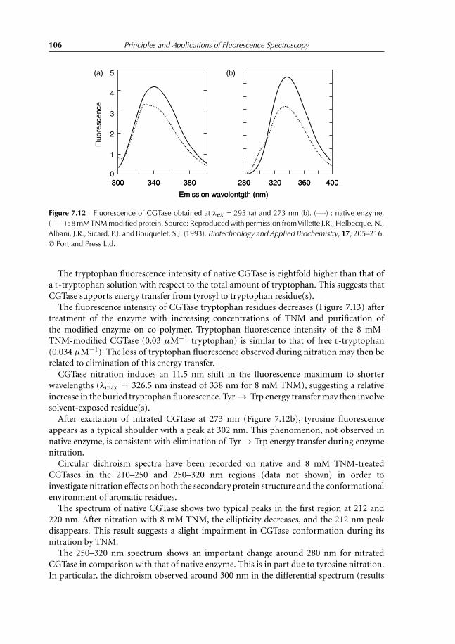
106 Principles and Applications of Fluorescence Spectroscopy
5
4
3
Flu
ores
cenc
e
2
1
0
(a) (b)
300300 340340 380380 280280 320320 360360 400400
Emission wavelentgth (nm)Emission wavelentgth (nm)
Figure 7.12 Fluorescence of CGTase obtained at λex = 295 (a) and 273 nm (b). (—-) : native enzyme,(- - - -) : 8mMTNMmodified protein. Source: Reproducedwith permission fromVillette J.R., Helbecque, N.,Albani, J.R., Sicard, P.J. and Bouquelet, S.J. (1993). Biotechnology andApplied Biochemistry, 17, 205–216.© Portland Press Ltd.
The tryptophan fluorescence intensity of native CGTase is eightfold higher than that ofa L-tryptophan solution with respect to the total amount of tryptophan. This suggests thatCGTase supports energy transfer from tyrosyl to tryptophan residue(s).
The fluorescence intensity of CGTase tryptophan residues decreases (Figure 7.13) aftertreatment of the enzyme with increasing concentrations of TNM and purification ofthe modified enzyme on co-polymer. Tryptophan fluorescence intensity of the 8 mM-TNM-modified CGTase (0.03 μM−1 tryptophan) is similar to that of free L-tryptophan(0.034 μM−1). The loss of tryptophan fluorescence observed during nitration may then berelated to elimination of this energy transfer.
CGTase nitration induces an 11.5 nm shift in the fluorescence maximum to shorterwavelengths (λmax = 326.5 nm instead of 338 nm for 8 mM TNM), suggesting a relativeincrease in the buried tryptophan fluorescence. Tyr → Trp energy transfer may then involvesolvent-exposed residue(s).
After excitation of nitrated CGTase at 273 nm (Figure 7.12b), tyrosine fluorescenceappears as a typical shoulder with a peak at 302 nm. This phenomenon, not observed innative enzyme, is consistent with elimination of Tyr → Trp energy transfer during enzymenitration.
Circular dichroism spectra have been recorded on native and 8 mM TNM-treatedCGTases in the 210–250 and 250–320 nm regions (data not shown) in order toinvestigate nitration effects on both the secondary protein structure and the conformationalenvironment of aromatic residues.
The spectrum of native CGTase shows two typical peaks in the first region at 212 and220 nm. After nitration with 8 mM TNM, the ellipticity decreases, and the 212 nm peakdisappears. This result suggests a slight impairment in CGTase conformation during itsnitration by TNM.
The 250–320 nm spectrum shows an important change around 280 nm for nitratedCGTase in comparison with that of native enzyme. This is in part due to tyrosine nitration.In particular, the dichroism observed around 300 nm in the differential spectrum (results

Fluorescence Spectroscopy Principles 107
3
2.5
2
Flu
ores
cenc
e in
tens
ity (
au)
1.5
1
0.5
0300 320 340
Emission wavelength (nm)
360 380 400
0
0.25
0.5
1
2
4
8
Figure 7.13 Tryptophan fluorescence spectra of CGTase after 18 h of nitration with 0, 0.25, 0.5, 1, 2,4, and 8 mM TNM. λex = 295 nm. Source: Villette J.R., Helbecque, N., Albani, J.R., Sicard, P.J. andBouquelet, S.J. (1993). Biotechnology and Applied Biochemistry, 17, 205–216. Reprinted with permissionfrom Portland Press.
Table 7.2 Absorption and fluorescence properties of tryptophan, tyrosine, phenylalanine, and the Y-base
Absorption Fluorescence
εmax(×10−3)
Fluorophore Conditions λmax (nm) (M−1 cm−1) λmax (nm) F τf (ns) Sensitivity
Trp H2O, pH 7 280 5.6 348 0.2 2.6 11Tyr H2O, pH 7 274 1.4 303 0.1 3.6 2Phe H2O, pH 7 257 0.2 282 0.04 6.4 0.08Y-base t-ARNPhe 320 1.3 460 0.07 6.3 0.91
From yeast
Reference: Cantor, C.R. and Schimmel, P.R. (1980). Biophysical Chemistry, W.H. Freeman, NewYork.
not shown) strongly suggests that the conformational environment of some tryptophanresidues has been changed during nitration.
These results support a conformational impairment of the enzyme during nitration andwould account for the loss of tryptophan fluorescence by the elimination of (Tyr → Trp)energy transfer (removal of the chromophores) and hence enzyme inactivation. Table 7.2lists the principal absorption and fluorescence characteristics of the three aromatic aminoacids within the proteins and of the Y-base.

108 Principles and Applications of Fluorescence Spectroscopy
Figure 7.14 Absorption spectra for (a) NADH (pH 7 buffer) and (b) NADH+ (pH 2 buffer).
7.3.2 Cofactors
NADH is highly fluorescent, with absorption and emission maxima located at 340 and450 nm, respectively, while NAD+ and NADH+ are not fluorescent (Figures 7.14 and 7.15).Schauenstein et al. (1980) explained the spectral modification of NADH+ by a higherpercentage of the stacked conformation at a lower pH.
FMN and FAD absorb light in the visible at 450 nm and fluoresce at around 515 nm. Thefluorescence lifetimes of FMN and FAD are 4.7 and 2.3 ns, respectively.
7.3.3 Extrinsinc fluorophores
7.3.3.1 Fluorescein and rhodamine
These bind covalently to lysines and cysteines of proteins, and absorb and fluoresce in thevisible. The fluorescence lifetimes of fluorescein and rhodamine are around 4 ns, and theiremission spectra are not sensitive to medium polarity.

Fluorescence Spectroscopy Principles 109
350 400 450 500 5500
2
4
6
8
10
12
14
16
18
Flu
ores
cenc
e in
tens
ity (
au)
Wavelength (nm)
a
b
Figure 7.15 Fluorescence emission spectra of (a) NADH (pH 7) and of (b) NADH+ (pH 2). λex = 340 nm.
7.3.3.2 Naphthalene sulfonate
5-((((2 iodoacetyl)amino)ethyl)amino)naphthalene-1-sulfonic acid (IAEDANS or 1,5-IAEDANS) and DNS bind covalently to proteins, while l-anilino-8-naphthalene sulfonate(ANS) and 2-p-toluidinylnaphthalene-6-sulfonate (TNS) bind non-covalently to proteinsand membranes. Dissolved in a polar medium such as water, TNS and ANS show a very weakfluorescence that increases with decreasing medium polarity. When bound to proteins or tomembranes, their fluorescence increases, and their maximum shifts to the blue edge. Theintensity increase and the shift to shorter wavelengths are increasingly important with thedecrease in binding-site polarity. Table 7.3 lists the characteristics of several extrinsic probes.
7.3.3.3 Nucleic bases
Puric and pyrymidic bases show a weak fluorescence in aqueous medium, which increasesby a factor of 10 in a medium of pH 2 and by a factor of 100 at 77 K. The quantum yieldof the nucleic acids depends largely on the temperature, and their fluorescence lifetime isweak. Fluorescence polarization is high, even at ambient temperature. At a low pH, theemission maximum is temperature-dependent.
Puric bases fluoresce at least three times more than pyrimidic bases. Guanidine is themost fluorescent basis. In the native state, DNA and RNA show a very weak fluorescence,

110 Principles and Applications of Fluorescence Spectroscopy
Table 7.3 Absorption and spectral properties of some used fluorophores
Absorption Emission
Fluorophore Binding site λmax (nm) εmax (×10−3) λmax f τf (ns)
Dansyl chloride Covalent bond 330 3.4 510 0.1 13on Cys and Lys
1,5-I-AEDANS Covalent bond 360 6.8 480 0.5 15on Lys and Cys
Fluorescein Covalent bond 495 42 516 0.3 4isothiocyanate (FITC) on lysines8-Anilino-1-naphthalene Noncovalent 374 6.8 454 0.98 16sulfonate (ANS) bond on proteinsPyrene and derivatives Membranes 342 40 383 0.25 100Ethidium bromide Noncovalent 515 3.8 600 1 26.5
bond on nucleicacids
Reproduced from Cantor, R.C. and Schimmel, P.R. (1980). Biophysical Chemistry,W.H. Freeman, NewYork. Fluorescencelifetimes are means.
to the difference of the yeast transfer RNA (t-RNA) that contains a highly fluorescent basiscalled Y basis.
At 77 K, the DNA and RNA fluorescence increases. This fluorescence is due to theformation of adenine and thymine dimers, while the fluorescence of guanine and cytosineis inhibited. Ethidium bromide, acridine and Hoechst 33258 intercalate between DNA andRNA bases, thereby inducing a fluorescence increase.
Ethidium bromide emits red fluorescence when bound to DNA. The fluorescentprobe is trapped in the base pair of DNA (Figure 7.16), thereby inducing an increasein its fluorescence intensity. Also, ethidium bromide can bind to double-stranded andsingle-stranded DNA and to RNA.
Hoechst 33258 binds to the minor groove of double-stranded DNA with a preferencefor the A–T sequence (Pjura et al. 1987). Interaction between DNA and proteins very ofteninduces structural modifications in both interacting molecules. Such modifications in DNAcan be characterized with 2-aminopurine (2AP), which is a highly fluorescent isomer ofadenine. 2AP does not alter the DNA structure. It forms a base pair with thymine and canbe selectively excited, since its absorption is red-shifted compared to that of nucleic acidsand aromatic amino acids. In addition, its fluorescence is sensitive to the conformationalchange that occurs within the DNA (Rachofsky et al. 2001).
7.3.3.4 Ions detectors
Some fluorophores are used to detect the presence of sodium or potassium in cells. Forexample, the maxima of the fluorescence excitation and emission spectra of SBFI increase,and its emission maximum shifts toward short wavelengths in the presence of sodium(Figure 7.17).

Fluorescence Spectroscopy Principles 111
FluorophoreBase pair
DNA
Ethidium bromideEtBr
H2N NH2
CH2CH3
N+ Br−
Figure 7.16 Binding of ethidium bromide to DNA.
a a
b
b
Flu
ores
cenc
e ex
cita
tion
Flu
ores
cenc
e em
issi
on
300 350 400 450 500 550 600 650
Wavelength (nm)
Figure 7.17 Fluorescence excitation (detected at 505 nm) and emission (excited at 340 nm) spectra ofSBFI in pH 7.0 buffer containing 135 mM (a) or zero (b) Na+. Source: Molecular Probes.
7.4 Polarity and Viscosity Effect on QuantumYield andEmission Maximum Position
Quantum yield and fluorescence emission maximum are sensitive to the surroundingenvironment. This can be explained as follows. Fluorophore molecules and amino acidsof the binding sites (in the case of an extrinsic fluorophore such as TNS, fluorescein, etc.)or the amino acids of their microenvironment (case of Trp residues) are associated by theirdipoles. Upon excitation, only the fluorophore absorbs the energy. Thus, the dipole of theexcited fluorophore has an orientation different from that of the fluorophore in the groundstate. Therefore, the fluorophore dipole–solvent dipole interaction in the ground state isdifferent from that in the excited state (Figure 7.18).

112 Principles and Applications of Fluorescence Spectroscopy
Absorption Fluorescence
E
S1
S1*
S0*
S0S0
Figure 7.18 Relationship between fluorescence emission and dipole orientation. Squares characterizefluorophore dipole and circles solvent dipole.
The new interaction is unstable. To reach stability, fluorophore molecules will use someof their energy to reorient the dipole of the microenvironment (solvent and surroundingamino acids). Dipole reorientation is called relaxation. Emission occurs after the relaxationphenomenon.
An important dipole means a high polarity. In this case, the energy released by thefluorophore to reorient the dipole of the microenvironment is very important. Therefore,for a highly polar environment, photon emission will occur with low energy and thus witha spectrum maximum shifted to higher wavelength.
In an apolar medium, fluorophore in the excited state will induce a dipole formationwithin the environment. The formation of a new dipole needs less energy than thereorientation of an already existing dipole. Thus, emission from an apolar environmentyields an emission spectrum with a maximum located in the blue compared to emissionoccurring in a polar environment.
Also, since the intensity and thus quantum yield are dependent on the number of emittedphotons, they will be lower when emission occurs in a polar environment. It should be notedhere that fluorescence parameters are more sensitive to the environment than absorptionspectra.
When a fluorophore is bound to a protein, its fluorescence will be dependent on thepolarity of the surrounding amino acids. Fluorescence spectra are also dependent onthe rigidity of the medium. The relaxation phenomenon (reorientation of the dipoleenvironment) occurs much more easily in a fluid medium. In such a case, emission will occurafter relaxation. This is the case when relaxation is faster than fluorescence, i.e., the relaxationlifetime τr is shorter than the fluorescence lifetime τ0. This occurs when the binding site isflexible, and the fluorophore can move easily. Emission from a relaxed state does not changewith excitation wavelength. This can be explained by the fact that whatever the value of theexcitation wavelength, the emission will always occur at the same energy level.

Fluorescence Spectroscopy Principles 113
When the binding site is rigid, fluorescence emission occurs before relaxation. Inthis case, excitation at the longer wavelength edge of the absorption band photoselectsthe population of fluorophores energetically different from that photoselected when theexcitation wavelength is shorter. In the absence of motions, specific excitation wavelengthwill reach specific population. Therefore, excitation at the red edge yields a fluorescencespectrum with a maximum located at a higher wavelength than that obtained when theexcitation occurs at short wavelengths. In other words, when surrounding environmentof the fluorophore is rigid, its emission maximum shifts to higher wavelengths with theexcitation wavelength.
In summary, the shift of the emission peak could be the result of two phenomena: thedecrease in the medium polarity and/or emission from a nonrelaxed state. Demchenko(1994) explains that:
applying the term hydrophobic to fluorophores is not correct, fluorophores are ratheramphipylic and posess a polar or even a charged group. Binding sites of these probes are notnecessary hydrophobic; however numerous data demonstrate that their short wavelength shiftof fluorescence spectra on binding is due to [the] slow rate of relaxations of the environmentrather than to its hydrophobic nature.
References
Albani, J.R. (2004). Structure and Dynamics of Macromolecules: Absorption and Fluorescence Studies,Elsevier, Amsterdam.
Albani, J.R. (2007). New insights in the interpretation of tryptophan fluorescence. Origin of thefluorescence lifetime and characterization of a new fluorescence parameter in proteins: theemission to excitation ratio. J. of fluorescence, in press.
Badea, M.G. and Brand, L. (1979). Time-resolved fluorescence measurements. Methods in Enzymology,61, 378–425.
Balabanli, B., Kamisaki, Y., Martin, E. and Murad, F. (1999). Requirements for heme and thiols for thenonenzymatic modification of nitrotyrosine. Proceedings of the Natural Academy of Sciences USA,96, 13136–13141.
Barik, A., Priyadarsini, K.I. and Mohan, H. (2003). Photophysical studies on binding of curcumin tobovine serum albumin. Photochemistry and Photobiology, 77, 597–603.
Bennett, R.G. (1960). Instrument to measure fluorescence lifetimes in the millimicrosecond region.Review of Scientific Instruments, 31, 1275–1279.
Burstein, E.A.,Vedenkina, N.S. and Ivkova, M. N. (1973). Fluorescence and the location of tryptophanresidues in protein molecules. Photochemistry and Photobiology, 18, 263–279.
Cantor, R.C. and Schimmel, P.R. (1980). Biophysical Chemistry, W.H. Freeman, New York.Demchenko, A.P. (1994). A new generation of fluorescence probes exhibiting charge-transfer
reactions. In: Proceedings of SPIE – The International Society for Optical Engineering, vol. 2137,588–599.
Froschle, M., Ulmer, W. and Jany, K.D. (1984). Tyrosine modification of glucose dehydrogenase fromBacillus megaterium. Effect of tetranitromethane on the enzyme in the tetrameric and monomericstate. European Journal of Biochemistry, 142, 533–540.
Handbook, Molecular Probes. 10th edn. (2005). http://probes.invitrogen.com/Jablonski, A. (1935). Über den Mechanismus des Photolumineszenz von Farbstoffphosphoren.
Zeitschrift fur Physik, 94, 38–64.

114 Principles and Applications of Fluorescence Spectroscopy
James, D.R., Siemiarczuk, A. and Ware, W.R. (1992). Stroboscopic optical boxcar technique for thedetermination of fluorescence lifetimes. Review of Scientific Instruments, 63, 1710–1716.
Lakowicz, J.R. (1999). Principles of Fluorescence Spectroscopy (2nd edn), Plenum, New York.Pjura, P.E., Grzeskowiak, K. and Dickerson, R.E. (1987). Binding of Hoechst 33258 to the minor
groove of B-DNA. Journal of Molecular Biology, 197, 257–271.Rachofsky, E.L., Osman, R. and Ross, J.B. (2001). Probing structure and dynamics of DNA with
2-aminopurine: effects of local environment on fluorescence. Biochemistry, 40, 946–956.Riordan, J.F., Wacker, W.E.C. and Vallee, B.L. (1966). Tetranitromethane. A reagent for the nitration
of tyrosine and tyrosyl residues of proteins. Journal of The American Chemical Society, 88,4104–4105.
Schauenstein, E., Saenger, W., Schaur, R.J., Desoye, G. and Schreibmayer, W. (1980). Influence of pH,temperature and polarity of the solvent on the absorption of NADH+ and NADH at 260 nm.Zeitschrift für Naturforschung C , 35, 76–79.
Spencer, R.D. (1970). Fluorescence lifetimes: theory, instrumentation and application of nanosecondfluorometry. Ph.D. thesis, University of Illinois at Urbana Champaign. Published by UniversityMicrofilms International.
Valeur, B. (2002). Molecular Fluorescence: Principles and Applications, Wiley-VCH, Weinheim.Villette, J.R., Helbecque, N., Albani, J.R., Sicard, P.J. and Bouquelet, S.J. (1993). Cyclomaltodextrin
glucanotransferase from Bacillus circulans E 192: nitration with tetranitromethane. Biotechnologyand Applied Biochemistry, 17, 205–216.

Chapter 8
Effect of the Structure and the Environmentof a Fluorophore on Its Absorption andFluorescence Spectra
Experiments
Students should read carefully the whole text before beginning the experiments and plottingthe spectra. The purpose of these experiments is to find out how the fluorophore structureaffects optical spectroscopy properties such as absorbance and fluorescence.
The following experiments have been chosen to provide students with experience withspectra of typical fluorescent molecules, which are often used in biochemical research.In particular, students should become familiar with the ways in which a molecule’senvironment can affect its energy states, and with the relation that exists between changesin energy states and the resulting modifications in absorption and fluorescence spectra.
Before entering the laboratory, students should be able to describe the following:
1 Absorption spectrum.2 Emission spectrum.3 Excitation spectrum.4 Relationship between 1, 2, and 3.5 Structures of ANS (1-anilinonaphthalene-8-sulfonate), L-tryptophan, riboflavin or
flavin, ethidium bromide (EB), TNS, and NADH.
Students should receive the following solutions:
• L-Trp in pH 7 buffer with an optical density at 295 nm equal to 0.12.• Riboflavin in pH 7 buffer with an optical density at 450 nm equal to 0.015.• Ethidium bromide in pH 7 buffer with an optical density at 480 equal to 0.153.• ANS in pH 7 buffer with an optical density at 350 nm equal to 0.06.• ANS in the presence of 10 μM of bovin serum albumin (optical density at 350 nm
should be around to 0.065).• TNS in pH 7 buffer with an optical density at 320 nm equal to 0.06.• TNS in the presence of 10 μM of bovin serum albumin (optical density at 320 nm
should be around to 0.065).• NADH dissolved in phosphate buffer pH 7 and in butylglycol (optical density should
be around 0.04 at 280 nm).

116 Principles and Applications of Fluorescence Spectroscopy
Figure 8.1 Normalized fluorescence emission spectrum (λex = 295 nm with emission peak = 355 nm)(c), excitation spectrum obtained at λem = 340 nm (b), and absorption spectrum (a) of L-tryptophan inphosphate buffer, pH 7.
Plot on the same graph paper the absorption spectrum of L-Trp solution from 240 to350 nm, the fluorescence emission spectrum from 300 to 450 nm (λex = 295 nm), and thefluorescence excitation spectrum from 240 to 350 nm (λem = 340 nm).
Plot on the same graph paper the absorption spectrum of the riboflavin solution from300 to 500 nm, fluorescence emission spectrum from 480 to 600 nm (λex = 450 nm) andthe fluorescence excitation spectrum from 300 to 500 nm (λem = 530 nm).
Plot on the same graph paper the absorption spectrum of ethidium bromide from 420to 580 nm, its fluorescence emission spectrum from 500 to 700 nm (λex = 475 nm) and itsfluorescence excitation spectrum from 420 to 580 nm (λem = 600 nm).
Plot on the same graph paper the absorption spectra from 240 to 450 nm, fluorescenceemission spectra from 360 to 550 nm (λex = 350 nm), and fluorescence excitation spectrafrom 240 to 450 nm (λem = 480 nm) of ANS and of ANS–BSA solutions.
Plot on the same graph paper, the normalized excitation (from 290 to 420 nm) (λem = 440or 450 nm) and emission spectra (from 360 to 560 nm) (λex = 340 nm) of NADH dissolved

Structure and the Environment of a Fluorophore 117
Figure 8.2 Normalized fluorescence emission spectrum (λex = 475 nm) with emission peak at 585 nm(©), excitation spectrum (λem = 600 nm (�)) and absorption spectrum (�) of ethidium bromide inphosphate buffer, pH 7.
in phosphate buffer pH 7 and in butylglycol and compare for both solvents, excitation peakstogether and emission peaks together.
For the solutions containing Trp, riboflavin, ethidium bromide, and ANS alone, normalizethe absorption and excitation spectra and superimpose them. We suggest that thenormalization be carried out at 280, 450, and 280 nm, for L-Trp, riboflavin, and ANS,respectively.
For the solution containing the ANS–BSA complex, normalize the absorption spectrumof free ANS in solution with the excitation spectrum of the ANS–BSA complex at 280 nmand superimpose them.
Questions:
1 Are the absorption spectra of the fluorophores identical? Explain.2 Are the fluorescence emission spectra of these fluorophores identical? Explain.3 Are the fluorescence excitation and absorption spectra of each fluorophore
superimposed? Explain.

118 Principles and Applications of Fluorescence Spectroscopy
Figure 8.3 Normalized fluorescence emission spectrum (λex = 450 nm with emission peak = 520 nm)(c), excitation spectrum (λem = 530 nm) (a) and absorption spectrum (b) of riboflavin in phosphate buffer,pH 7.
4 Are the fluorescence excitation spectrum of the ANS–BSA complex and the absorptionspectrum of the free ANS in solution superimposed? Explain.
5 Are the fluorescence excitation and absorption spectra of the ANS–BSA complexsuperimposed? Explain.
6 What will happen if you correct the fluorescence intensities of emission and excitationspectra for the inner filter effect?
7 Calculate the Stokes shift for each fluorophore.8 Plot the fluorescence emission spectra of ANS bound to serum albumin and of TNS (2,
p-toluidinylnaphthalene-6-sulfonate) also bound to the protein. Are the two spectraidentical? Explain.
9 Plot the fluorescence emission spectra of free TNS in solution (around 10–20 μM) inthe absence and presence of the same concentration of free tryptophan. What do youobserve? Can you explain the difference observed in the emission spectra obtained inparts 8 and 9?
10 Are the NADH spectra in good agreement with the polarity of the solvents used?

Structure and the Environment of a Fluorophore 119
Figure 8.4 Normalized fluorescence emission spectrum (λex = 350 nm with emission peak = 465 nm)(c), excitation spectrum (λem = 480 nm) (b) of ANS bound to BSA and absorption spectra (a) of free ANSin phosphate buffer, pH 7.
Answers:
1 The fluorophores show different absorption spectra since they possess differentstructures. In fact, the absorption spectrum reflects the electronic distribution of themolecule in the ground state and thus the molecule structure in the ground state.
2 The fluorophores show different fluorescence spectra. A fluorescence spectrum reflectsthe electronic distribution of the molecule in the excited state S1 and thus the structureof the molecule in this state. We notice also that ANS does not fluoresce in a phosphatebuffer (i.e., a polar medium), which is not the case when it is bound to serum albumin.Thus, fluorescence depends not only on the structure of the fluorophore but also onits environment. Each fluorophore has its own spectral properties, and one should becareful not to generalize a rule for all fluorophores, although most of the fluorophoresshare common rules.
3 Since ANS dissolved in a polar medium does not fluoresce, one cannot record itsfluorescence excitation spectrum. For tryptophan, ethidium bromide, and riboflavin,one can see that for each molecule, the absorption spectrum looks like the fluorescence

120 Principles and Applications of Fluorescence Spectroscopy
Figure 8.5 Normalized fluorescence emission spectra of the TNS–BSA complex (λex = 320 nm andλem = 432 nm) (a) and of ANS–BSA complex (λex = 350 nm and λem = 465 nm) (b).
excitation spectrum (Figures 8.1–8.3). In general, excitation and absorption spectraare supposed to superimpose when the fluorophore is in pure solution, and nodynamical or structural phenomena interface with it. This is true for fluorophores suchas ethidium bromide but not for L-Trp and riboflavin. In fact, although the generalfeature of excitation spectrum looks like the absorption spectrum, there is an importantdifference between the spectra recorded for L-Trp and riboflavin: the intensity of theexcitation spectrum does not vary with the wavelength in the same way them theoptical density along the absorption spectrum. Detailed studies of the phenomenonhave shown that absorption is not necessarily equal to excitation and thus fluorescenceemission spectra of fluorophores such as aromatic amino are proportional to theintensity of the excitation spectrum at the excitation wavelength and not to the opticaldensity at the excitation wavelength (Albani, 2007).
4 The absorption spectrum of free ANS in solution fluorescence excitation spectrumof the ANS–BSA complex do not overlap as a result of molecular interaction betweenANS and BSA (Figure 8.4). Energy transfer occurs between Trp residues of the BSA andANS molecules bound to the protein affecting the fluorescence excitation spectrum

Structure and the Environment of a Fluorophore 121
Figure 8.6 Emission spectra of buffer (a), free TNS (b), free TNS in the presence of free L-tryptophan (c)and of TNS bound to bovine serum albumin (d). λex = 320 nm.
of bound ANS. In fact, one can see that in the excitation spectrum of the complex,there is a peak at 280 nm characteristic of the protein. One can see also that there isa shift in the second peak of ANS absorption from 350 to 385 nm in the excitationspectrum. This shift also characterizes the difference in the structural environment ofANS (buffer and protein).
5 The absorption spectrum of ANS bound to serum albumin shows a peak at 370 nm,different from 350 nm observed for ANS alone and 385 nm observed in the excitationspectrum. In general, the excitation spectrum is much more accurate than theabsorption spectrum because it characterizes the real emitting fluorophores (hereANS bound to BSA). The absorption spectrum characterizes the sum of all absorbingmolecules in the different ground states, here free and bound ANS.
6 Corrections of the fluorescence excitation and emission spectra for the optical densities(inner filter effect) yield an increase in the intensities without inducing any shift inany of the maxima. This is true for all recorded spectra. At the optical densities weare suggesting, you may find that these corrections are not significant and even notnecessary for all fluorophores but ethidium bromide. Its intensity increases withoutany modification in the peak position.

122 Principles and Applications of Fluorescence Spectroscopy
Figure 8.7 Fluorescence excitation (a and b) and emission (c and d) spectra of NADH dissolved inphosphate buffer, pH 7 (full lines), and in butylglycol (dashed lines). λex = 360 nm and λem = 440 or450 nm. Peaks positions are: in phosphate buffer, 345 and 450 nm and in butylglycol, 355 and 437 nm.
7 The Stokes shift is equal to the distance (nm) that exists between the absorption andemission peaks:
Stokes shift = δλ = λem − λex (8.1)
The Stokes shift is dependent on the structure of the fluorophore itself and on itsenvironment (the solvent in which it is dissolved and/or the molecule to which it isbound. The Stokes shifts obtained are thus 75 nm (355–280 nm), 70 nm (520–450 nm),113 nm (585–472 nm), and 185 nm (465–280 nm) for tryptophan, riboflavin, ethidiumbromide, and ANS bound to BSA, respectively.
8 Figure 8.5 shows fluorescence emission spectra of TNS and ANS bound to serumalbumin. The two fluorophores do not show the same maximum, although the twofluorophores bind to hydrophobic domains of the protein. This result can be explainedmainly by the differences in the structure of the two fluorophores. Also, one couldexplain the difference in the emission peaks could be due to the higher sensitivityof TNS to hydrophobicity. This interpretation is based on the fact that the peak ofTNS emission spectrum is shifted to short wavelengths compared to that of ANS

Structure and the Environment of a Fluorophore 123
emission spectrum. However, this interpretation should be considered with caution,since effective comparative studies between the two fluorophores have not yet beenundertaken. The fluorescence excitation spectrum of the TNS–BSA complex (notshown), recorded at λem = 460 nm, a wavelength where only TNS emits, shows apeak located at 278 nm, characteristic of the protein absorption. This peak, absentin the absorption spectrum of TNS dissolved in buffer, indicates, as in the ANS–BSA complex, energy-transfer between tryptophan residues of serum albumin andTNS. The fluorescence intensity of fluorophores such as TNS and ANS increases whenthey bind to a protein or to a membrane. In a polar solvent such as water, the twofluorophores mainly TNS, do not show any significant fluorescence.
9 Figure 8.6 clearly indicates that in the presence of free tryptophan in solution, thereis no binding of TNS on the amino acid. However, in the presence of bovine serumalbumin, TNS shows a fluorescence emission spectrum, indicating that TNS is boundto the protein.
10 Regarding fluorescence excitation and emission spectra of NADH, Figure 8.7 showsthe normalized spectra obtained in phosphate buffer, pH 7, and in butylglycol. Theexcitation peak of NADH in phosphate buffer is located at 343–344 nm, while inbutylglycol it is located at 355 nm. This shift to higher wavelengths of the excitationpeak is the result of a low polarity of butylglycol compared to phosphate buffer. Thedifference in polarity also affects the emission position peak of NADH. In fact, emissionpeaks are located at 450 and 437 nm in phosphate buffer and butylglycol, respectively.
Reference
Albani, J.R. (2007). New insights in the interpretation of tryptophan fluorescence. Origin of thefluorescence lifetime and characterization of a new fluorescence parameter in proteins: theemission to excitation ratio. J. of fluorescence, in press.

Chapter 9Fluorophore Characterization andImportance in Biology
This chapter contains four experiments, which are to be conducted separately.
9.1 Experiment 1. Quantitative Determination of Tryptophan inProteins in 6 M Guanidine
9.1.1 Introduction
The luminescent properties of tyrosine and tryptophan are affected by theirmicroenvironments. Depending upon the location within the polypeptide structure and theneighboring charges, several classes of residues have been distinguished in native proteins(Cogwill 1968; Burstein et al. 1973). Each class exhibits mainly a distinct spectral emissionmaximum with a specific spectral bandwidth. Nevertheless, upon denaturation, the proteinunfolds, and, as was first reported by Teale (1960), for most proteins, the quantum yields oftryptophan residues tend to become uniform.
Fluorescence spectra of the tryptophanyl residues of the fully denatured protein isnormalized, as is its absorption spectra. In the absence of any structured protein,fluorescence of tryptophanyl residues and of free Trp in solution can be compared.
With an efficient denaturing agent such as guanidine hydrochloride (Tanford et al. 1966,1967) and in the presence of 2-mercaptoethanol, a more uniform environment could bereached and hence a normalization of the fluorescence parameters, a condition which hasto be met before applying the process for quantitative analytical purposes.
9.1.2 Principle
The analytical method proposed by Pajot (1976) involves (a) incubating the proteinof a known concentration in 6 M guanidine at pH 6.5–7 in the presence of 30 mM2-mercaptoethanol for 30 min (if only a small amount of the protein is available, theincubation can be carried out directly in the fluorescence cuvette); and (b) measuring thefluorescence, excited at 295 nm and observed at 354 nm, yielded by the denatured proteinin 6 M guanidine hydrochloride (tryptophanyl residues concentration 3–10 μM). A linearcalibration curve is obtained, thus allowing the ‘free tryptophan fluorescence equivalents’of the protein sample to be estimated by extrapolation.

Fluorophore Characterization and Importance in Biology 125
Therefore, by carrying out a titration as described above, the fluorescence of thedenatured protein can be compared to that of a given amount of free tryptophan.Plotting the fluorescence intensity at the emission maximum as a function of addedfree tryptophan residues allows the tryptophan concentration in the protein to bedetermined.
The fluorescence estimation may be impaired by the inner filter effect, but this maybe made practically negligible by lowering the sample concentration. A maximal totalconcentration of 25 μM tryptophan is correct, since about 98% of the incident light isthen available at the center of a 4-mm cell.
Although denaturation and the highly charged medium tend to make the fluorophoreenvironment uniform, certain features of the primary structure may exert some quenchingor enhancing effects on the fluorescence parameters of certain residues. This may be thecase with lysozyme, which contains a Trp–Trp segment, or with myoglobin, in whicha carboxylic charge is located on the amino acid adjacent to tryptophan. Such factorsmay be responsible for the deviation observed with some proteins. This type of studyalso relies upon the accuracy of the absorbance coefficients used for estimating proteinconcentrations.
9.1.3 Experiment
Prepare a 100 μM stock solution of L-Trp dissolved in 10 mM phosphate buffer. ε279 nm ofL-tryptophan is 5710 M−1 cm−1. Prepare stocks of 10 different proteins in 10 mM phosphatebuffer pH 7.
The concentration of each protein stock should be 25 μM. Incubate for 30 min, by slowlyshaking 40 μl of each protein stock in a fluorescence cuvette containing 860 μl of 6 Mguanidine, pH 7. The protein concentration in the cuvette is around 1 μM.
The stock of guanidine solution should be prepared in 0.1 M phosphate buffer.After 30 min of incubation, record the fluorescence spectrum for each protein from 310
to 440 nm, λex = 295 nm. Then, add to the cuvette at least 5 aliquots of 5 μl each from theL-Trp stock solution, and after each addition, record the fluorescence spectrum.
Plot the fluorescence intensity at the peak as a function of added L-Trp concentration, andthen determine the concentration of the tryptophan in the protein. From the concentrationof the protein you are using, you can determine the number of tryptophan present in eachprotein.
We suggest performing the experiments on the following proteins: rabbit muscle aldolase,A1%
280 = 9.38, Mr = 142 000; pig-heart aspartate aminotransferase, ε280 nm = 1.40 ×10⁵ M−1 cm−1 (dimer) and its apoenzyme ε280 nm = 1.33 × 10⁵ M−1 cm−1; bovineserum albumin, ε280 nm = 4.2 × 10⁴ M−1 cm−1; bovine α-chymotrypsin, A1%
282 = 20.4,Mr = 25 600; bovine α-chymotrypsinogen, A1%
280 = 21, Mr = 25 600; horse-heartcytochrome c , type VI, ε550 nm = 29.5 × 10³ M−1 cm−1; porcine cytochrome b5,ε556 nm = 27.5 × 10³ M−1 cm−1; bovine deoxyribonuclease, A1%
280 = 12.3, Mr = 31 000;bovine hemoglobin (Fe2+), ε555 nm = 12.5×10³ M−1 cm−1; muscle lactate dehydrogenase,ε280 nm = 20.1 × 10³ M−1 cm−1; β-lactoglobulin, ε278 nm = 17.6 × 10³ M−1 cm−1;egg lysozyme, ε280 nm = 37.8 × 10³ M−1 cm−1; sperm-whale myoglobin, ε409 nm =157×103 M−1 cm−1; porcine pepsin, ε278 nm = 50.9×10³ M−1 cm−1; bovine ribonuclease,

126 Principles and Applications of Fluorescence Spectroscopy
ε277.5 nm = 9800 M−1 cm−1; trypsin, A1%280 = 15.4, Mr = 23 891; soybean trypsin inhibitor,
A1%280 = 9.1; Mr = 21 700.
9.1.4 Results obtained with cytochrome b2 core
Figure 9.1 shows the fluorescence spectrum of tryptophan residues of cytochrome b2 coredissolved in 6 M guanidine, pH 7, in the presence of 30 mM 2-mercaptoethanol. Theemission peak is located at 357 nm, indicating that the protein is completely denatured(spectrum a). The fluorescence emission spectra of successive aliquots (0.55 μM) of freetryptophan added to the protein solution are also shown (spectra b–g).
Figure 9.1 Titration of 1 μM cytochrome b2 core in 6 M guanidine with aliquots of 5.5 μM of L-Trp.λex = 295 nm.
Figure 9.2 shows the fluorescence intensity maximum as a function of added freetryptophan. Extrapolation of the plot at the x-axis yields a value equal to 2 μM as theconcentration of tryptophan in the cytochrome b2 core. Since the protein concentrationin the cuvette is 1 μM, the number of tryptophan residues in the cytochrome b2 core is

Fluorophore Characterization and Importance in Biology 127
Figure 9.2 Determination of tryptophan residues concentration in the cytochrome b2 core.
2 μM/1 μM = 2. This value is identical to that known for cytochrome b2 core. In general,one should divide the value obtained by a correlation coefficient equal to 1.1 to obtain thereal number of tryptophan residues in the protein.
9.2 Experiment 2. Effect of the Inner Filter Effect onFluorescence Data
9.2.1 Objective of the experiment
Student will apply the Beer–Lambert–Bouguer law to find out the effect of the optical densityon the fluorescence intensity.This experiment can be performed with any fluorophore, butstudents should be sure that it is not aggregating beyond a specific concentration. This iswhy it is better to perform this experiment with a fluorophore that has a high exctinctioncoefficient, so that one can work at low concentrations. We have chosen fluorescein toperform the experiments.
9.2.2 Experiment
The same cuvette with each fluorescein concentration should be used to measure ODsat 495 nm and record the fluorescence intensities at 540 nm (λex = 495 nm). Preparea stock solution of at least 40 μM fluorescein. Calculate the volume you need to pipetteand to add to the fluorescence cuvette containing the buffer alone (1 ml of buffer forexample) so that you add aliquots of approximately 0.2 μM fluorescein to the cuvette.

128 Principles and Applications of Fluorescence Spectroscopy
Mix the solution, and then measure the OD and fluorescence intensity. Add aliquotsuntil you have 4 μM fluorescein in the cuvette. Plot the OD at 495 nm vs. fluoresceinconcentration. Do you obtain a linear plot? What is the value of ε you obtain fromyour data?
Plot the fluorescence intensity at 540 nm vs. the OD at 495 nm. How can you interpret theplot you obtained? With Equation (7.15), calculate the value of the fluorescence intensityat each OD. Superimpose your theoretical results with the experimental plot. What do youobserve?
9.2.3 Results
Figure 9.3 shows the variation in OD for fluorescein at 495 nm as a function of fluorophoreconcentration. We obtain a linear plot indicating that the Beer–Lambert–Bouguer law isrespected in this range of fluorescein concentrations. Since, in the present measurementsoptical densities were measured with a pathlength equal to 1 cm, we obtained at 495 nmfrom the slope of the plot, a value equal to 42 mM−1 cm−1 for ε. This result, identical to
Figure 9.3 Optical density (OD) of fluorescein at 495 nm as a function of chromophore concentration.

Fluorophore Characterization and Importance in Biology 129
Figure 9.4 Fluorescence intensity of fluorescein at 540 nm as a function of the optical density at theexcitationwavelength (495 nm). Plot (a) is the experimental, and plot (b) is calculated using Equation (7.15).
that known for fluorescein (see Table 7.3) means that the errors on the volume added andthus on the fluorescein concentrations in the cuvette are very small.
Plotting the fluorescein fluorescence intensity at 540 nm vs. the OD at the excitationwavelength (495 nm) does not yield a linear plot (Figure 9.4). Although we do not have anexplanation for the small curvarture at low fluorescein concentrations, results indicate thatlinearity between fluorescence intensities and ODs are clearly lost when the OD is higherthan 0.075. Corrections of the fluorescence intensities for the ODs at 495 nm (the inner filtereffect) indicate that up to an OD of 0.075, the theoretical fluorescence intensities are equalto the experimental intensities. When ODs are equal to or higher than 0.075, theoreticalfluorescence intensities are higher than the experimental intensities and are linear with thefluorescence intensities recorded for the lower ODs.
One can conclude that Equation (7.15) is very useful in correcting fluorescence intensitiesrecorded at high ODs. Also, it is important to indicate that the curvature observed, at highODs, in the experimental plot is not the result of fluorescein aggregation, since ODs increaselinearly with fluorescein concentrations (Figure 9.3).

130 Principles and Applications of Fluorescence Spectroscopy
9.3 Experiment 3. Theoretical Spectral Resolution of TwoEmitting Fluorophores Within a Mixture
9.3.1 Objective of the experiment
The objective of these experiments is to apply a method of calculation that allows, whenpossible, separation of the fluorescence spectra of two or three emitting residues. Instead ofusing a computer and applying specific programs, students will learn how to perform themathematical calculation and will see that it is very simple to obtain the different spectra.
The method we are asking the students to use is the ln-normal analysis of Burstein andEmelyanenko (1996).
In this analysis, the following equation is used:
I(ν) = Im exp{−(ln 2/ ln2 ρ) × ln2[(a − ν)/(a − νm)]} (9.1)
where Iνm = Im is the maximal fluorescence intensity. νm is the wavenumber of the bandmaximum,
ρ = (νm − ν−)/(ν+ − νm) (9.2)
is the band asymmetry parameter. ν+ and ν− are the wavenumber positions of the left andright half maximal amplitudes:
a = νm + Hρ/(ρ2 − 1) (9.3)
and H is the bandwidth:
H = ν+ − ν− (9.4)
Equation (9.1) allows us in principle to draw a spectrum that matches the entire spectrumobtained experimentally. This is correct only if the recorded spectrum originates fromone fluorophore (i.e., Trp in solution) or from compact protein within a folded structure.However, when the experimental spectrum originates from two fluorophores (i.e., mixturesof tyrosine and tryptophan in solution) or from a disrupted protein that has two classesof Trp residues, the calculated spectrum using Equation (9.1) does not match the recordedspectrum.
• Step 1: Students will record the fluorescence emission spectra of 10 μM L-Trp, 10 μML-Tyr, and around 160 μM Calcofluor.
• Step 2: Students will record the fluorescence spectrum of a (L-Trp + L-Tyr) mixture.• Step 3: Students will analyze emission spectra obtained in steps 1 and 2 using the Burstein
equation. For the fluorescence spectra recorded in step 1, the Burstein equation shouldyield theoretical spectra that match the recorded spectra. However, this will not be thecase for the tyrosine–tryptophan mixture.
• Step 4: Students will plot the fluorescence emission spectrum of the Trp residues of aprotein.
• Step 5: Students will analyze the emission spectra obtained in step 4 with the Bursteinequation. Correct the fluorescence spectrum for the inner filter effect before doing theanalysis with the Burstein–Emelyanenko method.

Fluorophore Characterization and Importance in Biology 131
We will show here the example of an analysis method concerning the fluorescenceemission of Calcofluor. First, with a Pasteur pipette, take a small amount of powder ofCalcofluor White and dissolve it in 1 ml of phosphate buffer present in the fluorescencecuvette. Then, measure the OD at 352.7 nm and calculate the fluorophore concentration inthe cuvette. The value of ε at this wavelength is 4388 M−1 cm−1. In principle, you shouldhave a Calcofluor solution concentration of 150–200 μM in the fluorescence cuvette.
Plot the fluorescence emission spectrum from 380 to 550 nm (λex = 300 nm). You willobtain the spectrum shown in Figure 9.5.
Figure 9.5 Experimental fluorescence emission spectrum of 160 μM calcofluor in water (full line) λex =300 nm, and that calculated theoretically (dashed line) using Equation (10.1).
Let us see the details of the equation we are going to use
I(ν) = Im exp{−(ln 2/ ln2 ρ) × ln2[(a − ν)/(a − νm)]} (9.1)
Im is the maximal intensity of the spectrum, i.e., at 438 nm, and is 19.5.
νm = 1/438 nm = 22.83 × 103 cm−1
ν− = 1/434 nm = 20.66 × 103 cm−1
ν+ = 1/410 nm = 24.4 × 103 cm−1

132 Principles and Applications of Fluorescence Spectroscopy
H = ν+ − ν− = 3.8 × 103 cm−1
ρ = (νm − ν−)/(ν+ − νm) = (22.83 − 20.66)/(24.4 − 22.83) = 2.17/1.57 = 1.382.
a = νm + Hρ/(ρ2 − 1) = 22.83 + (3.8 × 1.382)/0.909924 = 28.6 × 103 cm−1
Now that we have all the parameters values we need, we can replace them in Equation (9.1)and determine the value of the intensity I(ν) at a specific wavenumber (ν).
I(400 nm) = 19.5 exp{−(0.693/0.1046) × ln2[(28.6 − 25)/(28.6 − 22.83)]}= 19.5 exp[−6.625 × ln2(3.6/5.8)]= 19.5 × 0.2216 = 4.32 cm
The intensity measured at 400 nm from the spectrum is 3 cm, and that calculatedtheoretically is 4.32 cm. One can see that the two values are close. Let us do this alongthe emission wavelength:
λ (nm) I measured from the I calculatedrecorded spectrum (cm) theoretically (cm)
400 3 4.32410 9.8 9.77420 16 15.3430 19 18.86438 19.5 19.5450 17.6 18.3460 15.3 16.1470 13.1 13.7480 10.5 10.9490 8.3 8.8500 6.5 6.97510 4.9 5.4520 3.6 4.17530 2.6 3.15540 1.7 2.54
Now, let us plot the two spectra on the same graph. We shall obtain two identical spectrawith one peak at 438 nm (Figure 9.5).
9.3.2 Results
Figure 9.6 shows the emission spectrum of free L-Trp in solution.Figure 9.7 shows the experimental fluorescence spectrum of a mixture of L-tyrosine and
L-tryptophan in water (line, spectrum a). The presence of a small shoulder around 303 nmindicates that L-tyrosine contributes to the fluorescence emission. Analysis of the data using

Fluorophore Characterization and Importance in Biology 133
Figure 9.6 Experimental fluorescence emission spectrum of pure L-Trp in water (line) and that obtainedusing Equation (10.1) (�).
Figure 9.7 Experimental fluorescence emission spectrum of a mixture of L-tyrosine and L-tryptophanin water (line, spectrum a) and that approximated using Equation (9.1) (�, spectrum b). Substractingspectrum (b) from (a) yields a fluorescence spectrum (c) characteristic of tyrosine. λex = 260 nm.

134 Principles and Applications of Fluorescence Spectroscopy
Equation (9.1) yields a fluorescence spectrum (squares, spectrum b) that does not matchwith the experimental one, especially within the region where tyrosine emits. The calculatedspectrum (b) corresponds to that of tryptophan alone. Subtracting spectrum (b) from (a)yields a spectrum with a maximum at 303 nm corresponding to that of tyrosine.
Figure 9.8 shows the experimental fluorescence spectrum of Trp residues of 15 μMα1-acid glycoprotein (λex = 295 nm) (line) and calculated spectrum obtained usingEquation (9.1) (square). We notice that the calculated spectrum matches the experimentalspectrum. Note: students can apply this method to different fluorophore mixtures.
Figure 9.8 Experimental fluorescence emission spectrum of Trp residues of α1-acid glycoprotein (15 μM)(line) and that approximated using Equation (10.1) (�). λex = 295 nm.
9.4 Experiment 4. Determination of Melting Temperature ofTriglycerides in Skimmed Milk Using Vitamin A Fluorescence
9.4.1 Introduction
Ultraviolet absorption spectrum of vitamin A shows a maximum near 328 nm, which wasused extensively as a means for both identification and determination of the vitamin in the

Fluorophore Characterization and Importance in Biology 135
various natural sources in which it occurs. Different solvents such as alcohol, chloroform,benzene, and light petroleum have been used to study the effects of these solvents on thespectral properties of vitamin A from different oils and butter (Gillam and El Ridi 1938).
Vitamin A shows a fluorescence emission spectrum with a peak located at 450 nm. Sincefluorescence is more sensitive than absorption, vitamin A is retained in many foods suchas butter, oil, milk, and cheese, which retain the important quantities of vitamin A, andcan be studied by fluorescence spectroscopy. However, because of the thickness and densityof such products, classical right-angle spectroscopy studies are difficult to perform. In fact,high ODs at excitation and emission wavelengths may not only decrease the real fluorescenceintensity of the sample but also distort fluorescence spectra. We observed this fact when wetried to record the fluorescence emission spectrum of pure milk (spectrum not shown). Inorder to circumvent this problem, one should use front-face fluorescence spectroscopy. Inthis method, the sample is excited at the cuvette surface, thereby avoiding any displacementof the excitation light through the sample to the cuvette center (Figure 9.9). Therefore,the front-face technique yields fluorescence spectra (excitation and emission) that are notdistorted. In fact, with highly concentrated and opaque liquids, intensity measurements arenot reproducible or detectable. In the front-face technique, the excitation light is focused tothe front surface of the samples, and then fluorescence emission is collected from the sameregion at an angle that minimizes reflected and scattered light. Front-face spectroscopy isapplied to highly concentrated opaque or solid samples.
Sample
Emission Emission
Sample
Excitation
(a) (b)
Excitation
Figure 9.9 Principles of (a) right-angle and (b) front-face fluorescence spectroscopies.
The front-face technique was used by Dufour (2002) to study the melting point of amilk fat-in-water emulsion stabilized by β-lactoglobulin. Milk and milk products retainvitamin A located in the core and membrane of the fat globule. The lipids of milk fatglobules contain hundreds of triacylglycerol species. Increasing the temperature modifiesthe textural structures of these fat molecules and thus affects the fluorescence of vitamin A.Thus, vitamin A can be used as probe to follow structural changes within the fat particles andto study, if possible, their melting point. Figure 9.10 shows the excitation spectra of a milkfat-in-water emulsion at different temperatures and the ratios of the intensities at 322 and295 nm. The shape of the excitation spectra changes with temperature (Figure 9.10a). Themodification of the ratio I322/I295 with the temperature (Figure 9.10b), allows to determinethe melting point of the triglycerides found to be equal to 28◦C.

136 Principles and Applications of Fluorescence Spectroscopy
(a)
0.82.0
1.5
1.0
Flu
ores
cenc
e in
tens
ity 3
22nm
/29
nm
Flu
ores
cenc
e in
tens
ity (
au)
0.6
0.4
0.2
0.0280 300 320 10 20 30 40 50
Temperature (°C)Wavelength (nm)
(b)
Figure 9.10 (a) Excitation spectra of vitamin A of a milk fat-in-water emulsion (melting point of the fats:28◦C) recorded at (—) 8.3◦C, (· · · ) 13.8◦C, (- - -) 20.6◦C, (– - - –) 30.2◦C, and (——) 49.1◦C. (b) Changesin the ratio F322 nm/295 nm with temperature. Figure reprinted with permission from Dufour, E. (2002).American Laboratory, 2202 34, 51–55. Copyright © 2002 International Scientific Communnications, Inc.
9.4.2 Experiment to conduct
The experiment described in Figure 9.10 can be reproduced if front-face fluorescence isused. Otherwise, another experimental method should be applied to determine meltingpoint of triglycerides. The following method can be used. Add 15–20 μl of skimmed milkinto 1 ml of 1 N NaOH. The milk we used is enriched with vitamins E and B. By mixingslowly, you should soon obtain a clear and slightly pink solution.
Measure the fluorescence excitation intensity at 295 nm for increasing temperatures from7 to 40◦C, λem = 410 nm. Then, plot the fluorescence intensity vs. temperature. You shouldobtain an exponential decay curve. Finally, plot ln I vs. t ◦ and calculate the melting point.
9.4.3 Results
The fluorescence excitation spectrum of the milk–NaOH solution shows two maxima at280 and 325 nm (data not shown). Figure 9.11 shows the variation in fluorescence intensityat λex = 295 nm vs. temperature. The results clearly indicate that the fluorescence intensityis temperature-dependent and decreases exponentially with temperatures. Experimentsshould be repeated five times and performed on two different days. From the plot obtained,it is difficult to calculate the melting point of the triglycerides.
Therefore, we plot ln I vs. temperature. This should yield one straight slope (in theabsence of a melting point) or two slopes separated by an area where the slope is almostequal to zero. This area characterizes the transformation of the triglycerides from a solid-like state to a liquid state. Figure 9.12 clearly shows that we are in the presence of a meltingarea, indicating that fusion of triglycerides is not abrupt.
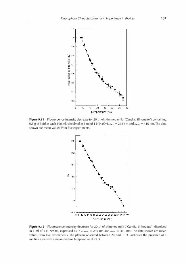
Fluorophore Characterization and Importance in Biology 137
Figure 9.11 Fluorescence intensity decrease for 20 μl of skimmed milk (“Candia, Silhouette”) containing0.1 g of lipid in each 100 ml, dissolved in 1 ml of 1 N NaOH. λex = 295 nm and λem = 410 nm. The datashown are mean values from five experiments.
Figure 9.12 Fluorescence intensity decrease for 20 μl of skimmed milk (“Candia, Silhouette”) dissolvedin 1 ml of 1 N NaOH, expressed as ln I . λex = 295 nm and λem = 410 nm. The data shown are meanvalues from five experiments. The plateau observed between 24 and 30 ◦C indicates the presence of amelting area with a mean melting temperature at 27 ◦C.

138 Principles and Applications of Fluorescence Spectroscopy
This result is in good agreement with that found by Dufour, and shows that alternativemethods to front-face fluorescence could be used. Our results indicate that a melting areaexists, and not only a single melting temperature. This means that structural changes occurwithin a temperature range where triglycerides are in a semi-solid–semi-fluid state. NaOHis used in general to neutralize the acid pH of milk. Finally, it is important to mention thatwe have not been able to dissolve non-skimmed (complete) milk in 1 N NaOH.
References
Burstein, E.A. and Emelyanenko, V.L. (1996). Log-normal description of fluorescence spectra oforganic fluorophores. Photochemistry and Photobiology, 64, 316–320.
Burstein, E.A., Vedenkina, N.S. and Ivkova, M.N. (1973). Fluorescence and the location of tryptophanresidues in protein molecules. Photochemistry and Photobiology, 18, 263–279.
Cogwill, R.W. (1968). Fluorescence and protein structure : XV. Tryptophan fluorescence in a helicalmuscle protein. Biochimica et Biophysica Acta, 168, 432–438.
Dufour, E. (2002). Examination of the molecular structure of food products using front-facefluorescence spectroscopy. American Laboratory, 34, 51–55.
Gillam, A.E. and El Ridi, M.S. (1938). The variation of the extinction coefficient of vitamin A withsolvent. The Biochemical Journal, 32, 820–825.
Pajot, P. (1976). Fluroescence of proteins in 6-M guanidine hydrochloride. A method for thequantitative determination of tryptophan. European Journal of Biochemistry, 63, 263–269.
Tanford, C., Kawahara, K. and Lapanje, S. (1966). Proteins in 6 M Guanidine Hydrochloride.Demonstration of random behaviour. Journal of Biological Chemistry, 241, 1921–1923.
Tanford, C., Kawahara, K. and Lapanje, S. (1967). Proteins as random coils. I. Intrinsic viscositiesand sedimentation coefficients in concentrated guanidine hydrochloride. Journal of the AmericanChemical Society, 89, 729–736.
Teale, F.W.J. (1960). The ultraviolet fluorescence of proteins in neutral solution. The BiochemicalJournal, 76, 381–388.
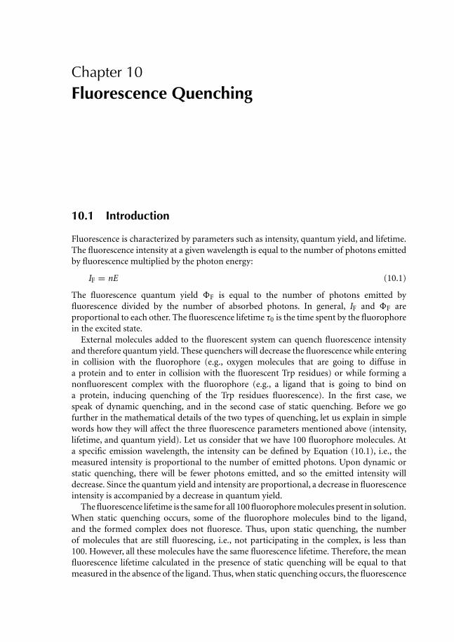
Chapter 10Fluorescence Quenching
10.1 Introduction
Fluorescence is characterized by parameters such as intensity, quantum yield, and lifetime.The fluorescence intensity at a given wavelength is equal to the number of photons emittedby fluorescence multiplied by the photon energy:
IF = nE (10.1)
The fluorescence quantum yield F is equal to the number of photons emitted byfluorescence divided by the number of absorbed photons. In general, IF and F areproportional to each other. The fluorescence lifetime τ0 is the time spent by the fluorophorein the excited state.
External molecules added to the fluorescent system can quench fluorescence intensityand therefore quantum yield. These quenchers will decrease the fluorescence while enteringin collision with the fluorophore (e.g., oxygen molecules that are going to diffuse ina protein and to enter in collision with the fluorescent Trp residues) or while forming anonfluorescent complex with the fluorophore (e.g., a ligand that is going to bind ona protein, inducing quenching of the Trp residues fluorescence). In the first case, wespeak of dynamic quenching, and in the second case of static quenching. Before we gofurther in the mathematical details of the two types of quenching, let us explain in simplewords how they will affect the three fluorescence parameters mentioned above (intensity,lifetime, and quantum yield). Let us consider that we have 100 fluorophore molecules. Ata specific emission wavelength, the intensity can be defined by Equation (10.1), i.e., themeasured intensity is proportional to the number of emitted photons. Upon dynamic orstatic quenching, there will be fewer photons emitted, and so the emitted intensity willdecrease. Since the quantum yield and intensity are proportional, a decrease in fluorescenceintensity is accompanied by a decrease in quantum yield.
The fluorescence lifetime is the same for all 100 fluorophore molecules present in solution.When static quenching occurs, some of the fluorophore molecules bind to the ligand,and the formed complex does not fluoresce. Thus, upon static quenching, the numberof molecules that are still fluorescing, i.e., not participating in the complex, is less than100. However, all these molecules have the same fluorescence lifetime. Therefore, the meanfluorescence lifetime calculated in the presence of static quenching will be equal to thatmeasured in the absence of the ligand. Thus, when static quenching occurs, the fluorescence

140 Principles and Applications of Fluorescence Spectroscopy
intensity and quantum yield decrease, and the fluorescence lifetime does not change. Directphysical interaction between the fluorophore and the ligand is not necessary to observestatic quenching. We can observe a long- or short-distance effect, depending on whetherthe fluorophore is within the interaction area or not.
Dynamic quenching does not induce complex formation; the fluorophore and quenchercollide, inducing a loss of fluorophore energy; and then the two molecules are againseparated. Thus, dynamic quenching induces a partial energy loss of the fluorophoremolecules entering into collision with the quencher molecules. This means that thefluorescence lifetime of these molecules is lower than for those free in solution and notparticipating in the dynamic process. Therefore, the mean fluorescence lifetime measuredin the presence of dynamic quenching will be lower than the mean lifetime measured in theabsence of the ligand. In conclusion, dynamic quenching induces a decrease in fluorescenceintensity, quantum yield, and lifetime. Also, one can observe a thermal quenching, whichis the decrease in the fluorescence parameters (lifetime, intensity and quantum yield) withtemperature. This decrease is dependent on the dynamics of the surrounding environmentof the fluorophore.
Förster energy transfer or energy transfer at a distance occurs between two molecules, adonor (the excited fluorophore), and an acceptor (a chromophore or fluorophore). Energyis transferred by resonance, i.e., the electron of the excited molecule induces an oscillatingelectric field that excites the acceptor electrons. As a result of this energy transfer, thefluorescence intensity and quantum yield of the emitter will decrease. Energy transfer isdescribed in Chapter 14.
10.2 Collisional Quenching: the Stern–Volmer Relation
Macromolecules display continuous motions. These motions can be of two main types: themolecule can rotate on itself, following the precise axis of rotation, and it can have a localflexibility. Local flexibility, also called internal motions, allows different small molecules,such as solvent molecules, to diffuse along the macromolecule. This diffusion is generallydependent on the importance of the local internal dynamics. Also, the fact that solventmolecules can reach the interior hydrophobic core of macromolecules such as proteinsclearly means that the term hydrophobicity should be considered as relative and not asabsolute. Internal dynamics of proteins allow and facilitate a permanent contact betweenprotein core and the solvent. Also, this internal motion permits small molecules such asoxygen to diffuse within the protein core. Since oxygen is a collisional quencher, analyzingthe fluorescence data in the presence of different oxygen concentrations yields informationon the internal dynamics of macromolecules.
Dynamic quenching occurs within the fluorescence lifetime of the fluorophore, i.e.,during the excited-state lifetime. This process is time-dependent. We have definedfluorescence lifetime as the time spent by the fluorophore in the excited state. Collisionalquenching is a process that will depopulate the excited state in parallel to the other processesalready described in the Jablonski diagram. Therefore, the excited-state fluorescence lifetimeis lower in the presence of a collisional quencher than in its absence.
The velocity of fluorophore de-excitation can be expressed as
v = kq[F ][Q] (10.2)

Fluorescence Quenching 141
where kq is the bimolecular quenching constant (M−1 s−1), [F] is the fluorophoreconcentration, which is held constant during the experiment, and [Q] is the quencherconcentration. If [Q] is higher than [F], the system can be considered as pseudo-first orderwith a constant equal to kq × [Q].
v = k ′[F ] = kq[Q][F ] (10.3)
The quantum yield in the absence of the quencher is
F = kr
kr + ki + kisc(10.4)
where kr is the radiative constant, kisc the intersystem crossing constant, and ki the constantcorresponding to de-excitation due to the temperature effect.
In the presence of a quencher, the quantum yield is
F(Q)= kr
kr + ki + kisc + kq[Q] (10.5)
F
F(Q)
= kr + ki + kisc + kq[Q]kr + ki + kisc
= kr + ki + kisc
kr + ki + kisc+ kq[Q]
kr + ki + kisc
= 1 + kq[Q] 1
kr + ki + kisc= 1 + kqτ0[Q] = 1 + KSV[Q]
(10.6)
where KSV is the Stern–Volmer constant, and τ0 is the mean fluorescence lifetime ofthe fluorophore in the absence of quencher. Equation (10.6) is called the Stern–Volmerequation.
Since the fluorescence intensity is proportional to the quantum yield, the Stern–Volmerequation can be written as:
I0
I= 1 + kqτ0[Q] = 1 + KSV[Q] (10.7)
where I0 and I are, respectively, the fluorescence intensities in the absence and presence ofquencher (Stern and Volmer 1919). Plotting I0/I as a function of [Q] yields a linear plotwith a slope equal to KSV.
The KSV value shows the importance of fluorophore accessibility to the quencher, whilethe value of kq gives an idea of the importance of the diffusion of the quencher withinthe medium. Figure 10.1 shows a Stern–Volmer plot of fluorescence intensity quenchingwith iodide of flavin free in solution and of flavin bound to flavocytochrome b2. The KSV
values found are 39 and 14.6 M−1 for free and bound flavins, respectively, i.e., values of kq
equal to 8.3 × 10⁹ and 3.33 × 10⁹ M−1 s−1, respectively. Accessibility of flavin to KI is moreimportant when it is free in solution, and the presence of protein matrix prevents frequentcollisions between iodide and FMN thereby decreasing the fluorophore accessibility to thequencher. Also, as revealed by the kq values, diffusion of iodide in solution is much moreimportant than in flavocytochrome b2. The protein matrix inhibits iodide diffusion, therebydecreasing the kq value.
Figure 10.2 shows a Stern–Volmer plot for the fluorescence intensity quenching by oxygenof zinc protoporphyrin IX embedded in the heme pocket of apomyoglobin (Mbdes →Fe).The slope of the plot yields KSV and kq values of 15.96 M−1 s−1 and 7.6 × 10⁹ M−1 s−1,
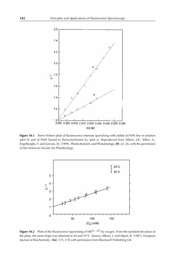
142 Principles and Applications of Fluorescence Spectroscopy
Figure 10.1 Stern–Volmer plots of fluorescence intensity quenching with iodide of FMN free in solution(plot b) and of FMN bound to flavocytochrome b2 (plot a). Reproduced from Albani, J.R., Sillen, A.,Engelborghs,Y. and Gervais, M. (1999). Photochemistry and Photobiology, 69, 22–26, with the permissionof the American Society for Photobiology.
20°C
35°C5
4
3
I 0 /
I
2
1
050 100
[O2] (mM)
150
Figure 10.2 Plots of the fluorescence quenching of MbFe→Zn by oxygen. From the standard deviation ofthe plots, the same slope was obtained at 20 and 35◦C. Source: Albani, J. and Alpert, B. (1987). EuropeanJournal of Biochemistry, 162, 175–178 with permission from Blackwell Publishing Ltd.

Fluorescence Quenching 143
respectively (τ0 = 2.3 ns). This kq value is lower than that (1.2 × 10¹⁰ M−1 s−1) foundfor oxygen when fluorescence-quenching of free tryptophan in solution with oxygen isperformed. This kq value is the highest value that can be measured in a homogeneousmedium. In the case of MbFe →Zn (Figure 10.2), the quenching constant, 7.6×10⁹ M−1 s−1,appears essentially to represent oxygen migration in and near the heme pocket andis temperature-independent. As a result of the short fluorescence lifetime of the zincporphyrin, τ0 = 2.1 ns, following dynamic quenching process of zinc-protoporphyrinfluorescence requires oxygen diffusion in spatial proximity to the fluorophore.
A Stern–Volmer plot can be obtained also from fluorescence lifetime quenching. In fact,the fluorescence lifetime in the absence of a quencher is
τ0 = 1
kr + ki + kisc(10.8)
and in the presence of a quencher, the fluorescence lifetime is
τQ = 1
kr + ki + kisc + kq[Q] (10.9)
τ0
τQ= 1 + kqτ0[Q] = 1 + KSV[Q] (10.10)
Equations (10.10) and (10.7) are identical. Therefore, in the presence of collisionalquenching, we have Equation (10.11) (Figure 10.3):
I0
I= τ0
τQ(10.11)
Figure 10.3 Stern–Volmer plot of quenching with oxygen of intensity and lifetime of protoporphyrin IXembedded in the heme pocket of myoglobin. Experiments performed at 20◦C.

144 Principles and Applications of Fluorescence Spectroscopy
The most common quenchers are oxygen, acrylamide, iodide, and cesium ions. The kq
value increases with probability of collisions between the fluorophore and quencher. Oxygenis a small and uncharged molecule, so it can diffuse easily. Therefore, the bimoleculardiffusion constant kq observed for oxygen in solution is the most important between allcited quenchers.
Acrylamide is an uncharged polar molecule, so it can diffuse within a protein andquenches fluorescence emission of Trp residues. The quencher should be able to collidewith tryptophan whether it is on the surface or in the interior of a protein. Nevertheless,Trp residues, mainly those buried within the core of the protein, are not all reached byacrylamide. For a fully exposed tryptophan residue or for Tryptophan free in solution, thehighest value of kq found with acrylamide is 6.4 × 10⁹ M−1 s−1.
Cesium and iodide ions quench Trp residues that are present at or near the surface of theprotein. The iodide ion is more efficient than the cesium ion, i.e., each collision with thefluorophore induces a decrease in fluorescence intensity and lifetime, which is not the casewith cesium. Also, since cesium and iodide ions are charged, their quenching efficiency willdepend on the charge of the protein surface. For free tryptophan and tyrosine in solution,the highest values of KSV that we have found with iodide are 17.6 and 19 M−1, respectively,and so the corresponding kq values are 6.8 × 10⁹ and 5.3 × 10⁹ M−1 s−1, respectively(Figure 10.4). KSV is calculated from the slope of the plot drawn at low KI concentrations.
Figure 10.4 Fluorescence intensity quenching of L-Trp by KI. Stock solution = 4 M KI + 10−3 Na2SO4.

Fluorescence Quenching 145
10.3 Different Types of Dynamic Quenching
When a protein possesses two or several Trp residues, when quenchers such as iodide,cesium, or acrylamide are used, and if all Trp residues are not accessible to the quencher,the Stern–Volmer equation yields a downward curvature. In this case, we have selectivequenching (Figure 10.5b). From the linear part of the plot, we can calculate the value ofthe Stern–Volmer constant corresponding to the interaction between the quencher andaccessible Trp residues. Upon complete denaturation and loss of the tertiary structure of aprotein, all Trp residues will be accessible to the quencher. In this case, the Stern–Volmer plotwill show an upward curvature. In summary, inhibition of the protein fluorescence withtwo or several Trp residues can yield three different representations for the Stern–Volmerequations, depending on the accessibility of the fluorophore to the quencher.
1 An exponential plot, i.e., all residues are accessible to the quencher or fluorescence isdominated by one single residue (Figure 10.5a).
2 Downward curvature, i.e., fluorescence is heterogeneous, and residues do not have anidentical accessibility to the quencher (Figure 10.5b).
3 Linear plot, i.e., fluorescence is heterogeneous and the accessibility of residues to theinhibitor slightly differs (Eftink and Ghiron 1976).
(a)
(b)
Figure 10.5 Acrylamide and CsCI quenching effects on the ascorbate oxidase emission properties. Steady-state (�) and dynamic (�) quenching of ascorbate oxidase by acrylamide (a) and CsCI (b) upon excitationat 293 nm. Source: Di Venere, A., Mei, G., Gilardi, G. et al. (1998). European Journal of Biochemistry,257, 337–343 with permission from Blackwell Publishing Ltd.

146 Principles and Applications of Fluorescence Spectroscopy
In a selective quencher, the fluorophores fraction accessible to the quencher canbe calculated. Let us consider two populations of fluorophore, one accessible to thequencher and the second inaccessible. At high quencher concentrations, fluorescence ofthe accessible fluorophores is completely quenched. Thus, residual fluorescence originatesfrom inaccessible fluorophores, i.e., fluorophores buried in the hydrophobic core of theprotein.
The fluorescence intensity F0 recorded in the absence of quencher is equal to the sumof the fluorescence intensities of populations accessible (Fa) and inaccessible (Fb) to thequencher:
F0 = Fa + Fb (10.12)
In the presence of quencher, only fluorescence of the accessible population decreasesaccording to the Stern–Volmer equation. The fluorescence recorded at a defined quencherconcentration [Q] is
F = F0(a)
1 + KSV[Q] + F0(b)(10.13)
where Ksv is the Stern–Volmer constant of the accessible fraction:
F0 − F = �F = F0(a) × KSV[Q]1 + KSV[Q] (10.14)
F
�F= F0 + F0 × KSV[Q]
F0(a) × KSV[Q] = F0
F0(a) × KSV[Q] + F0
F0(a)
(10.15)
F0
�F= 1
fa × KSV[Q] + 1
fa(10.16)
where fa is the fraction of the accessible fluorophore population to the quencher. Therefore,if one plots F0/�F vs. 1/[Q], a linear plot is obtained whose slope is 1/faxKSV, and theintercept is equal to 1/fa. Equation (10.16) is known as the Lehrer equation (Lehrer 1971).
Accessibility of a fluorophore to the solvent and thus to the quencher depends onits position within the protein. For example, buried Trp residues should have a loweraccessibility to the solvent than those present at the surface.
Figure 10.6 shows fluorescence emission spectra of lens culinaris agglutinin (LCA)(a) (λmax = 330 nm), of inaccessible Trp residues (b) (λmax = 324 nm) obtainedby extrapolating to [I−] = ∞, and of quenched Trp residues (c) obtained bysubtracting spectrum (b) from spectrum (a). The emission maximum of accessibleTrp residues is located at 345 nm, a characteristic of emission from Trp residues nearthe protein surface. Thus, both classes of Trp residues contribute to the fluorescencespectrum of LCA (Albani 1996). The presence of five Trp residues makes the analysisby the modified Stern–Volmer equation very approximate; nevertheless, a selectivequenching method allows the percentage of accessible fluorophores to the quencher to bedetermined.
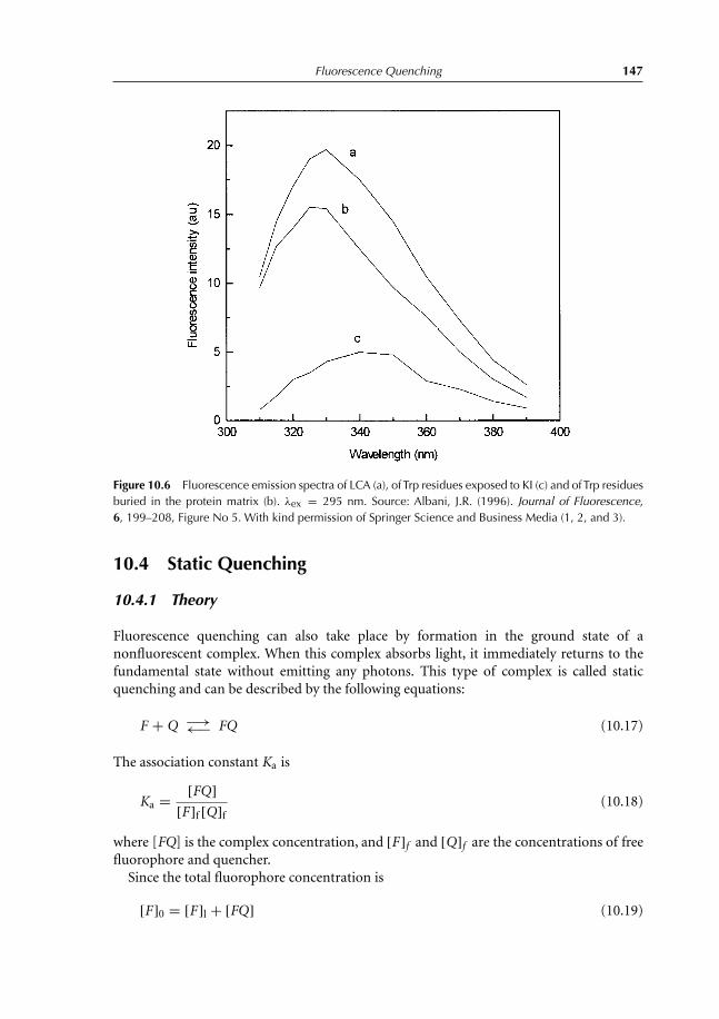
Fluorescence Quenching 147
Figure 10.6 Fluorescence emission spectra of LCA (a), of Trp residues exposed to KI (c) and ofTrp residuesburied in the protein matrix (b). λex = 295 nm. Source: Albani, J.R. (1996). Journal of Fluorescence,6, 199–208, Figure No 5. With kind permission of Springer Science and Business Media (1, 2, and 3).
10.4 Static Quenching
10.4.1 Theory
Fluorescence quenching can also take place by formation in the ground state of anonfluorescent complex. When this complex absorbs light, it immediately returns to thefundamental state without emitting any photons. This type of complex is called staticquenching and can be described by the following equations:
F + Q −→←− FQ (10.17)
The association constant Ka is
Ka = [FQ][F ]f [Q]f
(10.18)
where [FQ] is the complex concentration, and [F ]f and [Q]f are the concentrations of freefluorophore and quencher.
Since the total fluorophore concentration is
[F ]0 = [F ]l + [FQ] (10.19)
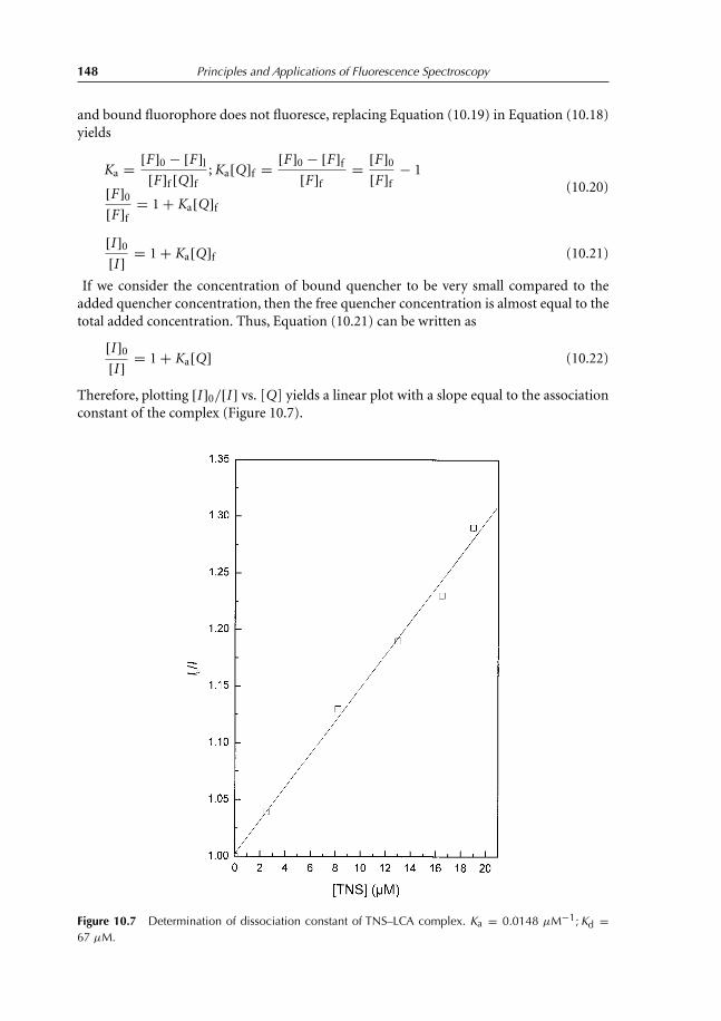
148 Principles and Applications of Fluorescence Spectroscopy
and bound fluorophore does not fluoresce, replacing Equation (10.19) in Equation (10.18)yields
Ka = [F ]0 − [F ]l
[F ]f [Q]f; Ka[Q]f = [F ]0 − [F ]f
[F ]f= [F ]0
[F ]f− 1
[F ]0
[F ]f= 1 + Ka[Q]f
(10.20)
[I ]0
[I ] = 1 + Ka[Q]f (10.21)
If we consider the concentration of bound quencher to be very small compared to theadded quencher concentration, then the free quencher concentration is almost equal to thetotal added concentration. Thus, Equation (10.21) can be written as
[I ]0
[I ] = 1 + Ka[Q] (10.22)
Therefore, plotting [I ]0/[I ] vs. [Q] yields a linear plot with a slope equal to the associationconstant of the complex (Figure 10.7).
Figure 10.7 Determination of dissociation constant of TNS–LCA complex. Ka = 0.0148 μM−1;Kd =67 μM.

Fluorescence Quenching 149
Lectins are widely used as tools in the study of plasma membrane modifications inneoplasia. Lectins are able to bind sugars specifically, but the binding constant of the specificfree sugar with a lectin may be several orders of magnitude lower than the binding constantof a glycoconjugate containing this sugar. LCA is primarily specific for α-mannopyranosylresidues. The lectin recognizes α-mannopyranosyl end-groups or those substituted at the0–2 position. Additional requirements for strong binding involve the presence of an L-fucoseresidue α-1,6-linked to an N -acetylglucosamine (GlcNac) which is linked to the protein viaa N-glycosamine bond. This lentil lectin is a mixture of two proteins named LCH-A andLCH-B.
In static quenching, one observes fluorescence of free fluorophore in solution. Complexedfluorophore does not fluoresce and is not observed in the derived equations. Thefluorescence lifetime of free fluorophore is the same whether all fluorophore moleculesare free or some are complexed. Thus, the fluorescence lifetime of fluorophore does notchange upon increasing the quencher concentration. This implies the following equation:
τ0/τ(Q) = l (10.23)
Therefore, in static quenching, one observes an intensity decrease only. Binding of TNSto α1-acid glycoprotein induces a decrease in the fluorescence intensity of the protein Trpresidues. Fluorescence lifetime of the intrinsic fluorophore is not modified. Variations inTrp residue intensities and lifetimes can be analyzed by plotting intensities and lifetimes inthe absence and presence of TNS as a function of TNS concentration (Figure 10.8). It isclear from the figure that the TNS–α1-acid glycoprotein interaction is of a static nature.
Figure 10.8 Quenching of the tryptophan fluorescence of α1-acid glycoprotein (4 μM) by TNS at 20◦C.Intensity (a) and lifetime (b) variation. Reproduced from Albani, J.R., Sillen, A., Engelborghs, Y. andGervais, M. (1999). Photochemistry and Photobiology, 69, 22–26, with permission of theAmerican Societyfor Photobiology.

150 Principles and Applications of Fluorescence Spectroscopy
0
6
5
4
3
2
1
050 100 150
35°C20°C
15°C
[O2] (mM)
I 0/I
Figure 10.9 Stern–Volmer plots of the fluorescence intensity quenching of MbdesFe by oxygen. The kτ0values were obtained from the initial slopes of each plot. Source: Albani, J. and Alpert, B. (1987). EuropeanJournal of Biochemistry, 162, 175–178 with permission from Blackwell Publishing Ltd.
In static quenching, an intrinsic or extrinsic fluorophore is used to examine theinteraction between two macromolecules.
The fluorophore should be bound to one of the two proteins only (case of extrinsicfluorophores) or should be part of it (case of intrinsic fluorophores). Also, the bindingparameters of the fluorophore–macromolecule complex can be determined by followingthe fluorescence modification of the fluorophore observables.
Finally, one should remember that dynamic quenching is diffusion-dependent, whilestatic quenching is not. Thus, a temperature increase induces an increase in the diffusioncoefficient and of kq (Figure 10.9). However, in the presence of static quenching, increasingthe temperature destabilizes the formed complex and thus decreases its association constant(Figure 10.10).
As the slopes of the Stern–Volmer plots are equal to kτ0, and since the fluorescencelifetimes, τ0, of both porphyrins do not change with temperature, the slope variation reflectsa change that occurs in oxygen diffusion with the temperature. From the slopes at lowquencher concentrations, we have found values of k equal to 8.4 ± 0.4 × 10⁸ M−1 s−1 and13 ± 0.4 × 10⁸ M−1 s−1 at 20◦ and 35◦C, respectively.
Figure 10.10 shows the interaction between TNS and the α1-acid glycoprotein. Wenotice that for a constant protein concentration, fluorescence intensity is higher at lowtemperatures. The Ka obtained is 19.6(±4)×103 M−1, 16.7(±3)×103 M−1, and 11(±2)×103 M−1 at 10, 20, and 33◦C, respectively. The maximal fluorescence of the complexdecreases with increasing temperature (301 ± 60, 201 ± 30, and 156 ± 30, respectively,in arbitrarily scaled units), as expected from the known temperature dependence ofnonradiative decay processes (Albani et al. 1995).
Finally, the formation of a complex in the fundamental state can be characterized bydisruption of the absorption spectrum of one of the two molecules that forms the complex(Schaberle et al. 2003).
Fluorescence quenching is frequently applied to sudy the interaction between humicacids and pollutants. Before presenting one or two applications, we will describe briefly

Fluorescence Quenching 151
Figure 10.10 Fluorescence intensity of TNS (0.85 μM) in the presence of increased concentration ofα1-acid glycoprotein. (a) = 9◦C. (b) = 20◦C. (c) = 33.5◦C. λex = 320 nm and λem = 430 nm.
some of the terminology used in ecotoxicology. We call bioavailability, fraction of chemicalcomponent present in the environmental medium and which is available to be accumulatedby the organisms. The environment can include water, sediments, particles in suspension,and food. According to the mode of action and the quantity of pollutant in the medium, twotypes of toxicity can be observed: acute and chronic toxicities. Acute toxicity describes theadverse effects resulting from a single exposure to a substance (The MSDS HyperGlossary:).Chronic toxicity leads to organisms mortality. Chronic toxicity leads to long-term effects andis evaluated by different types of effects measurements (reproduction, distortions, growthdelay…) (Gourlay, 2004).
The hydrophobicity of an organic molecule is quantified by means of its partitioncoefficient between octanol and water (KOW). KOW is equal to the ratio of compoundconcentrations at saturation in n-octanol and in water at equilibrium and at a specifictemperature. n-Octanol possesses structural properties analogous to lipidic tissues oforganisms, and so KOW allows evaluation of the lipophilic character of the contaminant andthus of its capacity to be accumulated in the lipidic tissues of living organisms. The KOW
value of hydrophobic organic pollutants (HOPs) is higher than 100. They are nonpolarmolecules with a low water solubility. Their weak solubility and their hydrophobicity

152 Principles and Applications of Fluorescence Spectroscopy
lead them to bind preferentially on hydrophobic particles of the medium, composed ofparticulate organic matter (POM) and dissolved organic matter (DOM). POM is organicmatter that is retained on a 0.45 μm sieve. It consists of living organisms (phytoplankton,bacteria, and animals) and detritus (e.g., biogenic material in various stages ofdecomposition).
DOM is composed of small molecules that can be obtained by filtration. Quantificationof organic matter in aquatic environment is performed by measuring the concentrationsexpressed in organic carbon. One measures total organic carbon (TOC) obtained from rawliquid sample, particulate organic carbon (POC) by analyzing the filter, and the dissolvedorganic carbon (DOC) characterized from the sample after filtration.
Humic substances are the main components of DOM. Thus, the presence of humicsubstances within the aqueous environment decreases the toxicity level. Organic matter isgenerally characterized by its absorption located in the range 254–280 nm.
According to their acidity, humic substances are hydrophobic and are split into twogroups: humic and fulvic acids. Humic acids are stable molecules originating from theageing of organic matter. They are responsible for water coloration and represent 40–60%of natural organic matter in rivers and lakes. Fulvic acids are smaller than the humicacids and are generally less aromatic than humic acids extracted from the same poolof DOM.
Soil acidity originates from parental material (quartz, granite, sandstone, etc.), fromorganic matter (fulvic and humic acids, etc.), and from the pedogenetic evolution. In fact,acidity occurs not only from the presence of H+ ions but also from Al3+ ions. Rootsexchange some H+ ions by Ca2+ and Mg2+ ions and acidify the medium.
Humic acids are polymerized organic acids of loose structure, which makes themhydrophilic. They are large dark brown or gray-black molecules and are in general richin oxygen and carbon, and some contain calcium that helps them to bind to clay inducing ahumic-clay complex. They are formed in soil by oxidization of the lignin and polyphenolsinducing their polymerization. Fulvic acids are poor in carbon and rich in nitrogen, andare found in poorly aerated acidic media. Dervived from the Latin fulvus, meaning yellow,fulvic acids have the same properties as humic acids but are composed of smaller moleculesand are less polymerized.
Humic substance has a complex structure, comprising a hydrophobic core carryingfunctional radicals, mainly carboxyls and hydroxyls. Thus, humic substances can react withdifferent products of various chemical functions, and so they interact ecologically with allclasses of toxic products such as heavy metals, pesticides, etc.
The hydrophobic character of organic pollutants means that they can be adsorbedby sediments or particles in suspension or bind to DOMs such as humic substances.The hydrophobicity of organic pollutants reduces the probability of finding them free inwater.
In the presence of very hydrophobic pollutants, three phases can be considered: water,DOM, and POM. Thus, the presence of DOM decreases the bioavailability and thusthe harmfulness of the POHs. Only organic pollutants dissolved and free in water arebioavailable for organisms.
Humic substances that constitute the hydrophobic part of DOM have a high capacity forsorption of hydrophobic organic pollutants. Humic acids have a better sorption capacitythan fulvic acids, and thus reduce bioaccumulation much better than fulvic acids.

Fluorescence Quenching 153
Increasing HSconcentration
250
200
150
100
Flu
ores
cenc
e in
tens
ity
50
Pyrene
360 380 400 420� (nm)
440 460 4800
Figure 10.11 Variation of fluorescence emission spectra of pyrene with increasing the humic substanceconcentration. Source: Frimmel, H.F. (2000). Agronomie, 20, 451–463. Authorization of reprint accordedby INRA, France.
2.2
1.8
1.4
F0/F
10 1 2
Concentration of HS ×106 (kg C l−1)
3 4 5
Pyrene
Fluoranthene
Anthracene
Figure 10.12 Binding constants analysis for quenching of pyrene, fluoranthene, and anthracenefluorescence with Aldrich HS. Reprinted with permission from Perminova, I., Grechishcheva, N. andPetrosyan,V. (1999). Environmental Science andTechnology, 33, 3781–3787. Copyright © 1999AmericanChemical Society.
Figure 10.11 shows the fluorescence emission spectrum of pyrene in the absence andpresence of two humic substance concentrations. The fluorescence intensity of pyrenedecreases with increasing humic substance concentration. This decrease results from thebinding of pyrene on the humic substance.
Binding of pyrene,fluoranthene,and anthracene to humic substances has been performedby following the decrease in fluorescence intensity of the polluants in the presence ofincreased humic substance concentrations. Figure 10.12 shows an analysis of the databased on calculations using Equation (10.22). Since the slopes of the plots are equal tothe association constants of the complexes, one can say that pyrene has the highest affinityto humic substances, followed by fluoranthene and anthracene.

154 Principles and Applications of Fluorescence Spectroscopy
4
3pH 4
pH 11
4
3
2
1
� F0/�
F
2I F
0 /I F
1
1 5 10 15
DOC (mg l−1)
20 25 30 35
Figure 10.13 Determination of the association constant of a humic substance – pollutants at two pH.Source: Frimmel, H.F. (2000).Agronomie, 20, 451–463.Authorization of reprint accorded by INRA, France.
Binding studies between humic substances and polluants have also been performed byfollowing the variation in fluorescence lifetime for the polluant as a function of increasedconcentration of humic substances. Binding means static quenching, and so no variationin the fluorescence lifetime should be observed (Figure 10.13).
We can see that while the fluorescence intensity of the polluant is modified in the presenceof DOM (DOC), its lifetime does not change. Thus, we have static quenching. Dissolvedorganic matter–hydrophobic polluant interactions are pH-dependent. In fact, DOC areacids, and so at high pHs, their structure could be modified, and their interaction withhydrophobic polluant would decrease.
10.5 Thermal Intensity Quenching
De-excitation of a fluorophore occurs via different competitive mechanisms described in theJablonski diagram. The global rate constant, which is the inverse of the fluorescence lifetime,can be considered equal to the sum of the different rates of the competitive mechanisms.Thus, one can write:
1/τ0 = kr + kisc + ki +∑
kqi (10.24)
where kr is the radiative constant, kisc the intersystem crossing constant, ki the constantcorresponding to de-excitation due to the temperature effect, and
∑kqi the different
quenching mechanisms such as proton transfer or electron transfer. In the presence ofenergy transfer at a distance (Förster energy transfer), another rate constant, kT, should beadded.
Working at a constant temperature allows the different parameters of the system to becontrolled, and one can quantify the mechanisms intervening in the depopulation of thefluorophore excited state. However, what will happen when we measure the fluorescencelifetime or intensity at different temperatures? Free in solution, a fluorophore can betemperature-dependent or not. In the first case, the temperature variation affects both

Fluorescence Quenching 155
lifetime and intensity. In the second case, none of these parameters is affected. Thetemperature increase favors important Brownian motions facilitating energy loss viadynamic quenching by the solvent. This will induce a decrease in the fluorescence quantumyield and in parallel with fluorescence intensity. Fluorescence lifetime is less sensitiveto temperature than the quantum yield, and so the observed decrease in fluorescencelifetime with temperature is not proportional to that observed for quantum yield orintensity.
With a temperature increase, kr decreases. kisc is temperature-independent, and sothe temperature will not affect kr. The constant ki or thermal constant increases withtemperature. ki is called the solvent constant, since the latter is considered to be responsiblefor the temperature dependence of the fluorescence lifetime. ki allows fluorophore activationenergy to be determined by the classical Arrhenius theory:
ki = A exp(−E/RT ) (10.25)
where A is the temperature-independent factor equal to 1015–1017 s−1. E is the Arrheniusactivation energy (kcal mol−1), R is the molar gas constant, and T is the temperature inkelvins. Plotting ln ki as a function of 1/T yields the value of E . Taking into considerationthat not all constant rates are temperature-dependent, and neglecting the presence of energytransfer, Equation (10.24) can be simplified to
1/τ0 = kr + ki (10.26)
Thus, Equation (10.25) can be written as
ki = 1/τ − kr = A exp(−E/RT ) (10.27)
Since the fluorescence lifetime can be obtained experimentally and kr calculated, the valueof E can be obtained by plotting ln(1/τ − kr) as a function of 1/T . One should notethat since kr is at least 10 times less than 1/τ , it is no longer taken into account inEquation (10.27).
Figure 10.14 displays fluorescence lifetime and quantum yield of FMN with temperaturein the absence and presence of AMP. Figure 10.15 shows the Arrhenius plot of free FMN insolution obtained with Equation (10.27).
The slope of fluorescence lifetime variation with temperature of FMN in the absence ofAMP differs from that observed in the presence of AMP, thus indicating that an interactionexists between FMN and AMP. The quantum yield of FMN free in solution varies identicallyto fluorescence lifetime. However, in the presence of AMP, the quantum yield increases, whilethe lifetime decreases, thus indicating that a static complex (nonfluorescent) is formedbetween FMN and AMP.
The activation energy of FMN is 0.77 kcal mol−1, a smaller value than that(4.2 kcal mol−1) found for NADH in the same conditions. This clearly means that thedifference in the radiotionless transitions is characteristic of the structures of the studiedcompounds.
The activation energy of the FMN–AMP complex has also been determined and foundto be equal to 5.6 kcal mol−1, thus revealing that the structure around the fluorophore andthe nature of the interaction between the two molecules will also play an important role inthe definition of the activation energy.

156 Principles and Applications of Fluorescence Spectroscopy
Figure 10.14 Fluorescence lifetime (a and c) and quantum yield (b and d) of free FMN in solution (a andb) and of FMN in the presence of AMP (c and d). The values of the quantum yields are normalized withthose of lifetime in order to make a better comparison between the two variations in parameters. Adaptedfrom Spencer, R.D. (1970). Ph.D. thesis, University of Illinois at Urbana Champaign.
3.2
18.9
18.8
lnk s
°
18.73.3 3.4
1000 temperature
3.5 3.6
k2 = 1.47 × 10⁸ s−1
�a = 0.77 × kcal mol−1A = 5.5 × 10⁸ s−1
Arrhenius parameters at 20°C
Figure 10.15 Arrhenius plot of the rate of radiationless transitions of FMN in water. Source: Spencer, R.D.(1970). Ph.D. thesis, University of Illinois at Urbana Champaign.
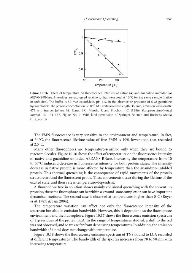
Fluorescence Quenching 157
1
0.9F/F
10
0.8
10 20 30
Temperature [°C]
Figure 10.16 Effect of temperature on fluorescence intensity of native (�) and guanidine unfolded (•)AEDANS-RNase. Intensities are expressed relative to that measured at 10◦C for the same sample (nativeor unfolded). The buffer is 50 mM cacodylate, pH 6.5, in the absence or presence of 6 M guanidinehydrochloride.The protein concentration is 10−5 M. Excitation wavelength: 350 nm; emission wavelength:476 nm. Source: Jullien, M., Garel, J-R., Merola, F. and Brochon J.-C. (1986). European BiophysicalJournal, 13, 131–137, Figure No. 1. With kind permission of Springer Science and Business Media(1, 2, and 3).
The FMN fluorescence is very sensitive to the environment and temperature. In fact,at 34◦C, the fluorescence lifetime value of free FMN is 10% lower than that recordedat 2.5◦C.
Many other fluorophores are temperature-sensitive only when they are bound tomacromolecules. Figure 10.16 shows the effect of temperature on the fluorescence intensityof native and guanidine unfolded AEDANS-RNase. Increasing the temperature from 10to 30◦C induces a decrease in fluorescence intensity for both protein states. The intensitydecrease in native protein is more affected by temperature than the guanidine-unfoldedprotein. This thermal quenching is the consequence of rapid movements of the proteinstructure around the fluorescent probe. These movements occur during the lifetime of theexcited state, and their rate is temperature-dependent.
A fluorophore free in solution shows mainly collisional quenching with the solvent. Inproteins, the same fluorophore can be within a ground-state complex or can have importantdynamical motions. The second case is observed at temperatures higher than 0◦C (Royeret al. 1987; Albani 2004).
The temperature variation can affect not only the fluorescence intensity of thespectrum but also its emission bandwidth. However, this is dependent on the fluorophoreenvironment and the fluorophore. Figure 10.17 shows the fluorescence emission spectrumof Trp residues of the protein LCA. In the range of temperatures studied, a shift to the redwas not observed, and so we are far from denaturing temperatures. In addition, the emissionbandwidth (54 nm) does not change with temperature.
Figure 10.18 shows the fluorescence emission spectrum of TNS bound to LCA recordedat different temperatures. The bandwidth of the spectra increases from 78 to 98 nm withincreasing temperature.

158 Principles and Applications of Fluorescence Spectroscopy
280 300 320 340 360 380 400 420 440 460
0
5
10
15
20
i
a
Flu
ores
cenc
e in
tens
ity (
au)
Wavelength (nm)
Figure 10.17 Fluorescence spectra of Trp residues of LCA at different temperatures. λex = 295 nm.Spectruma: 6.5◦C. Spectrumb: 9.5◦C. Spectrumc: 12◦C. Spectrumd: 15◦C. Spectrume: 17.8◦C. Spectrumf: 20.4◦C. Spectrum g: 23◦C. Spectrum h: 26◦C. Spectrum i: 30◦C.
350 400 450 500
0
2
4
6
8
10
12
14
16
18
20
22
9
1
Flu
ores
cenc
e in
tens
ity (
au)
Wavelength (nm)
Figure 10.18 Fluorescence spectra of TNS bound to LCA as a function of temperature. λex = 320 nm.Spectrum 1: 6.5◦C. Spectrum 2: 9.5◦C. Spectrum 3: 12◦C. Spectrum 4: 15◦C. Spectrum 5: 17.8◦C.Spectrum 6: 20.4◦C. Spectrum 7: 23◦C. Spectrum 8: 26◦C. Spectrum 9: 30◦C.
Fluorescence Quenching 159
References
Albani, J. and Alpert, B. (1987). Fluctuation domains in myoglobin. Fluorescence quenching studies.European Journal of Biochemistry, 162, 175–178.
Albani, J., Vos, R., Willaert, K. and Engelborghs, Y. (1995). Interaction between human α1-acid glycoprotein (orosomucoid) and 2-p-toluidinylnaphthalene-6-sulfonate. Photochemistry andPhotobiology, 62, 30–34.
Albani, J.R. (1996). Dynamics of Lens culinaris agglutinin studied by red-edge excitation spectra andanisotropy measurements of 2-p-toluidinylnaphthalene-6-sulfonate (TNS) and of tryptophanresidues. Journal of Fluorescence, 6, 199–208.
Albani, J.R. (2004). Effect of the secondary structure of carbohydrate residues of α1-acid glycoprotein(orosomucoid) on the local dynamics of Trp residues. Chemistry and Biodiversity, 1, 152–160.
Albani, J.R., Sillen, A., Engelborghs, Y. and Gervais, M. (1999). Dynamics of flavin in flavocytochromeb2: a fluorescence study. Photochemistry and Photobiology, 69, 22–26.
Di Venere, A., Mei, G., Gilardi, G. et al. (1998). Resolution of the heterogeneous fluorescence inmulti-tryptophan proteins: ascorbate oxidase. European Journal of Biochemistry, 257, 337–343.
Eftink, M.R. and Ghiron, C.A. (1976). Exposure of tryptophanyl residues in proteins. Quantitativedetermination by fluorescence quenching studies. Biochemistry, 15, 672–680
Frimmel, H.F. (2000). Development in aquatic humic chemistry. Agronomie, 20 ,451–463.Gourlay, C. (2004). Biodisponibilité des hydrocarbures polycycliques dans les écosystèmes aquatiques:
influence de la matière organique naturelle et anthropique. Thèse de doctorat à l’Ecole Nationaledu Génie Rural, des Eaux et Forêts Centre de Paris.
Jullien, M., Garel, J-R., Merola, F. and Brochon J.-C. (1986). Quenching by acrylamide and temperatureof a fluorescent probe attached to the active site of ribonuclease. European Biophysical Journal, 13,131–137.
Lehrer, S.S. (1971). Solute perturbation of protein fluorescence. The quenching of the tryptophylfluorescence of model compounds and of lysozyme by iodide ion. Biochemistry, 10, 3254–3263
Perminova, I., Grechishcheva, N. and Petrosyan, V. (1999). Relationships between structure andbinding affinity of humic substances for polycyclic aromatic hydrocarbons: relevance of moleculardescriptors. Environmental Science and Technology, 33, 3781–3787.
Royer, C.A., Tauc, P., Hervé, G. and Brochon, J.-C. (1987). Ligand binding and protein dynamics:a fluorescence depolarization study of aspartate transcarbamylase from Escherichia coli.Biochemistry, 26, 6472–6478.
Schaberle, F.A., Kuz’min, V.A. and Borissevitch, I.E. (2003). Spectroscopic studies of the interactionof bichromophoric cyanine dyes with DNA. Effect of ionic strength. Biochimica Biophysica Acta,1621, 183–191.
Spencer, R.D. (1970). Fluorescence lifetimes: theory, instrumentation and application of nanosecondfluorometry. Ph.D. thesis, University of Illinois at Urbana Champaign. Published by UniversityMicrofilms International, Ann Arbor, MI.
Stern, O. and Volmer, M. (1919). Uber die Abklingungszeit der Fluoreszenz. Physikalische Zeitschrift,20, 183–188.

Chapter 11Fluorescence Polarization
11.1 Definition
Biological systems show global rotation and local dynamics that are dependent on thestructure, environment, and function of the system. These motions differ from one systemto another, and within one system, local motions are not the same. The best-known exampleis that of membrane phospholipids where the hydrophilic phosphates are rigid, and thehydrophobic lipid is highly mobile. Polarized light is a good tool for studying differenttypes of rotations a molecule can undergo.
Natural light is unpolarized; it has no preferential direction. Thus, in order to studymolecules dynamics during the excited-state lifetime, molecular photoselection should beperformed. This can be reached by exciting the fluorophores with a polarized light andby recording the emitted light in a polarized system. When excitation is performed withpolarized light (definite orientation), absorption of the fluorophore will depend on theorientation of its dipole in the ground state compared to the polarized excitation light(Figure 11.1).
Fluorophores with dipoles perpendicular to excitation light will not absorb. Fluorophoreswith dipoles parallel to excitation light will absorb the most. Thus, polarized excitation willinduce photoselection in the fluorophore absorption. The electric vector of excitation lightis oriented parallel to or in the same direction as the z-axis. Emitted light will be measuredwith a polarizer. When emission is parallel to the excitation, the measured intensity is calledI‖. When the emission is perpendicular to the excitation light, the measured intensity iscalled I⊥. Light polarization and anisotropy are obtained according to Equations (11.1)and (11.2):
P = I‖ − I⊥I‖ + GI⊥
(11.1)
and
A = I‖ − I⊥I‖ + 2GI⊥
(11.2)
G is the correction factor and allows one to take into account the differences in sensitivityof the detection system in the two polarizing directions Ivv and Ivh. The G factor can be

Fluorescence Polarization 161
c
aE
b
hcva
hcva
Ip Iv
(a) (b)
Figure 11.1 Photoselection of differently oriented molecules with plane-polarized (a) and unpolarized(b) light. Excited molecules are shaded. After Albrecht, A.C. (1961). Journal of Molecular Spectroscopy,6, 84. Figure published by Dörr, F. (1971), Creation and Detection of the Excited States, pp. 53–122,Dekker, NewYork.
evaluated by measuring the fluorescence intensities parallel and perpendicular to the z-axiswith the excitation polarizer perpendicular to the z-axis. G will be equal to:
G = Ivh
Ihh(11.3)
P and A are inter-related with the following two equations:
P = 3A
2 + A(11.4)
and
A = 2P
3 − P(11.5)
Since the presence of polarizers induces photoselection, the global fluorescence intensityrecorded in the presence of polarizers is lower than that obtained in their absence. This is aconsequence of the decrease in the number of absorbing and emitting fluorophores.
A fluorophore free in solution can have a low polarization value, whereas when it is boundto a macromolecule, its polarization increases. The polarization unit is a dimensionlessentity, i.e., the value of P does not depend on the intensity of emitted light and thefluorophore concentration. However, this is the theory; the reality is quite different. Infact, measuring polarization at high fluorophore concentrations yields erroneous values,and in many cases, instead of reading the correct values of P and A, values that neighborthe limiting values are recorded.
Equation (11.1) indicates that values of P occur between 1 (I⊥ = 0) and −1 (I‖ = 0).Natural or unpolarized light, where I⊥ = I‖, yields a P value of 0. These two extremevalues of P are observed when the polarized absorption transition moment and that of theemission are colinear (I⊥ = 0) or perpendicular (I‖ = 0). However, in a rigid mediumwhere motions are absent, the absorption and emission transition dipoles can be orientedby an angle θ , one relative to the other.

162 Principles and Applications of Fluorescence Spectroscopy
Therefore, the probability of light absorption by the molecules will be a function of cos2 θ ,and the polarization will be equal to
Po = 3 cos2 θ − 1
cos2 θ + 3(11.6)
and
Ao = 3 cos2 θ − 1
5(11.7)
θ Po Ao
0 0.5 0.445 0.14 0.154.7 0.00 0.0090 −0.33 −0.20
A value of θ = 0 indicates that the excitation and emission dipoles are co-planar. This meansthat excitation induces an S0 → S1 transition. For an angle of 54.7◦, P and A are 0. Thisangle is called the “magic angle.” By measuring fluorescence emission with polarizers setup with an orientation equal to the magic angle, unpolarized light can be detected. Po andAo are called, respectively, intrinsic polarization and anisotropy. Po and Ao are measuredat temperatures equal to −45◦C or less. At this temperature, fluorophores do not showany movement. Colinear excitation and emission vectors yield S0 → S1 and S1 → So
transitions. This means that high positive values of P would correspond to an S0 → S,transition, while negative values of P would correspond to the So → S2 transition.
Since electronic transitions differ from one excitation wavelength to another, the valueof P would change with excitation wavelength. Emission generally occurs from the lowestexcited state S1v0, and so one can measure anisotropy or polarization along the absorptionspectrum at a fixed emission wavelength. We obtain a spectrum called the excitationpolarization spectrum or simply the polarization spectrum (Figure 11.2).
Figure 11.2 shows the excitation polarization spectrum of protoporphyrin IX in propyleneglycol at −55◦C (full line) and bound to the heme pocket of apohemoglobin recorded at20◦C (dotted line). One can see that polarization at a low temperature is higher than thatobserved when porphyrin is embedded in the heme pocket of apohemoglobin. This is theresult of fluorophore local motions within the pocket, independently of the global rotationof the protein.
Finally, it is important to mention that the polarization spectrum shape is characteristicof the chemical structure and nature of the fluorophore.
11.2 Fluorescence Depolarization
11.2.1 Principles and applications
In vitrified solution and/or when fluorophore molecules do not show any residual motions,the measured polarization is equal to the intrinsic one, Po. This value is obtained at low

Fluorescence Polarization 163
350
0.4A(o) / Ao = 1−
0.3
0.2
0.1
Pol
ariz
atio
n
0
−0.4
400 450 500
� (nm)
550 600
cos = (1− — )1/223
Figure 11.2 Excitation polarization spectrum of protoporphyrin IX in propylene glycol at−55◦C (full line)and bound to the heme pocket of apohemoglobin recorded at 20◦C (dotted line). λem = 634 nm. Source:Sebban P. (1979). Etude par fluorescence de molécule HbdesFe thesis, University of Paris 7.
and ambient temperatures, too, if, during the excited-state lifetime of the fluorophore, i.e.,during the time period between light absorption and emission, the orientation of excitationand emission dipoles does not change.
However, during the excited-state lifetime, energy transfer to neighboring moleculesand/or local and global motions of the fluorophores can be observed. These two phenomenainduce reorientation of the emission dipole, thereby depolarizing the system. Therefore, thevalue of the measured polarization P will be lower than intrinsic polarization value Po
(Weber, 1952).The relationship between P and Po is given by the Perrin equation:
1
P− 1
3=
(1
Po− 1
3
) (1 + RTτo
ηV
)=
(1
Po− 1
3
) (1 + τo
φR
)(11.8)
where R is the gas constant = 2.10 kcal mol−1 deg−1 or 0.8 × 10³ g cm2 s−2 M−1 deg−1;T , the temperature in kelvins; η the medium viscosity in centipoise (cp) or g cm−1 s−1
(1 cp = 0.01 g cm−1 s−1); and V and φR the rotational volume and rotational correlationtime of the fluorophore.
Plotting 1/P as a function of T/η yields in principle a linear graph with a y-interceptequal to 1/Po and a slope equal to
Rτo
V
(1
Po− 1
3
)The Perrin plot can also be written as
1
A= 1
Ao
(1 + τo
φR
)(11.9)
Decreasing the temperature or increasing the concentration of sucrose and/or glycerol inthe medium increases the medium viscosity.

164 Principles and Applications of Fluorescence Spectroscopy
Whether fluorophores are intrinsic or extrinsic to the macromolecule (protein, peptide,or DNA), depolarization is the result of two motions, fluorophore local motions andmacromolecule global rotation.
Rotational correlation time of a spherical macromolecule can be determined usingEquation (11.10) or Equation (11.11):
φP = M (ν + h)η/kTN (11.10)
where M is the molecular mass, v = 0.73 cm3 g−1 characterizes the specific volume,h = 0.3 cm3 g−1 is the hydration degree, η is the medium viscosity, and N is the Avogadronumber.
φP(T ) = 3.8η(T ) × 10−4 M (11.11)
Equations (11.10) and (11.11) do not yield exactly the same value for φP. For example, fora protein with a molecular mass of 235 kDa, such as flavocytochrome b2extracted from theyeast Hansenula anomala, the rotational correlation times calculated from Equations (11.10)and (11.11) are 97 and 90 ns, respectively.
The Perrin plot enables us to obtain information concerning fluorophore motion. Whenthe fluorophore is tightly bound to the protein, its motion will correspond to that of theprotein. In this case, φR will be equal to the protein rotational correlation time φP, andAo obtained experimentally from the Perrin plot will be equal to that measured at −45◦C(Figure 11.3).
The rotational correlation times measured at 15◦C and 35◦C are equal to 5.5 and3.6 ns. These values, within the range of theoretical values of myoglobin, indicate thatzinc porphyrin is tightly linked to the myoglobin heme pocket. The extrapolated value of Pis 0.176. This value, identical to that (0.1744) measured for the polarization Po at −20◦C,does not reveal the presence of motions. Thus, Perrin plot experiments show that zinc-protoporphyrin IX is rigid within the heme pocket. This result is in good agreement withthat found by Raman spectroscopy. In fact, the authors found that the zinc–imidazole bondis anomalously weak, orientation of the proximal histidine is suboptimal for binding to thezinc, and it is held relatively rigid in the myoglobin heme pocket (Andres and Atassi 1970).
When fluorophore exhibits local motions, extrapolated value of A, A(o), is lower thanthe Ao value obtained at −45◦C. Information obtained from the Perrin plot slope dependson the fluorophore fluorescence lifetime and on the relative amplitudes of the fluorophoreand protein motions.
Equation (11.9) indicates the possibility of calculating the rotational correlation time ofthe fluorophore not only by varying the T/η ratio but also by adding a collisional quencher.Interaction between the quencher and fluorophore decreases the fluorescence lifetime andintensity of the fluorophore, and increases its fluorescence anisotropy. Plotting 1/A as afunction of τo yields a straight line with a slope equal to φR. If the fluorophore is tightlybound to the macromolecule and does not exhibit any residual motions, the measured φR isequal to φP, and the extrapolated anisotropy is equal to that measured at a low temperature.
If, however, the fluorophore exhibits free motion, the measured φR is lower than that ofthe protein, and extrapolated anisotropy is lower than the limiting anisotropy.

Fluorescence Polarization 165
Figure 11.3 Steady-state fluorescence polarization vs. temperature/viscosity ratio for MbFe→Zn. Datawere obtained by thermal variation of temperature. λex = 517 nm and λem = 600 nm.
11.3 Fluorescence Anisotropy Decay Time
Anisotropy measurements yield information on molecular motions taking place during thefluorescence lifetime. Thus, measuring the time-dependent decay of fluorescence anisotropyprovides information regarding rotational and diffusive motions of macromolecules (Wahland Weber, 1967). Time-resolved anisotropy is determined by placing polarizers in theexcitation and emission channels, and measuring the fluorescence decay of the parallel andperpendicular components of the emission.
In the time-decay method, fluorescence anisotropy can be calculated as follows:
A(t ) = D(t )/S(t ) (11.12)
where
D(t ) = Vv = gVH (11.13)
S(t ) = Vv + 2gVH (11.14)
Vv and VH are fluorescence intensities of vertically and horizontally polarized components,respectively, obtained with vertically polarized light. g is the correction factor and is equal
166 Principles and Applications of Fluorescence Spectroscopy
to HV/HH, where HV and HH are the vertically and horizontally polarized components,respectively, of the fluorescence elicited by horizontally polarized light.
For a fluorophore bound tightly to a protein, anisotropy decays as a single exponential,
A(t ) = Aoe−t P (11.15)
where P is the rotational correlation time of the protein, and Ao is the fluorophore intrinsicanisotropy at the excitation wavelength.
When a fluorophore exhibits segmental motions, time-resolved anisotropy decay mustbe analyzed as the sum of exponential decays:
A(t ) = Ao[αe−t/φS + (1 − α)e−t/φL ] (11.16)
where φS and φL are the short and long rotational correlation times, α and 1 − α are theweighting factors for the respective depolarizing processes.
1
φS= 1
φP+ 1
6φF(11.17)
and
1
φL= 1
φP(11.18)
F is the rotational correlation time of the fluorophore.
11.4 Depolarization and Energy Transfer
Energy transfer is a source of depolarization. For example, a high energy-transfer efficiencyin hemoproteins can be evidenced by plotting Perrin plot at different temperatures.
The cytochrome b2 core from the yeast Hansenula anomala has a molecular mass of14 kDa, and its sequence shows the presence of two tryptophan residues. Their fluorescenceintensity decay can be adequately described by a sum of three exponentials. Lifetimesobtained from the fitting are equal to 0.054, 0.529, and 2.042 ns, with fractional intensitiesequal to 0.922, 0.068, and 0.010. The mean fluorescence lifetime, τo, is 0.0473 ns.
The main fluorescence lifetime (τ=54 ps) and its important fractional intensity (fi =92%) indicate that an important energy transfer occurs between Trp residues and heme.In an attempt to measure rotational correlation time of the protein, we have measuredanisotropy of cytochrome b2 core Trp residues at different temperatures. Results aredescribed with the classical Perrin plot (1/A as a function of T/η) (Figure 11.4).
The data yield a rotational correlation time equal to 38 ps instead of 5.9 ns calculatedtheoretically for the cytochrome b2 core, with an extrapolated value A(o) of 0.208, lowerthan that (0.265) usually found for Trp residues at λex = 300 nm at −45◦C. The fact thatthe extrapolated anisotropy is lower than the limiting anisotropy means that the system isdepolarized as a result of global and local motions within the protein. In this case, the valueof the apparent rotational correlation time (A) calculated from the Perrin plot is lowerthan the global rotational time of the protein (P). However, the fact that A is 1000 timeslower than P indicates that a third process different than the global and local rotations is

Fluorescence Polarization 167
Figure 11.4 Steady-state fluorescence anisotropy vs. temperature/viscosity ratio for tryptophan residuesof cytochrome b2 core. Data are obtained by thermal variations in the range 10–36◦C.
participating in the depolarization of the system. This process is the high energy transferthat occurs from the tryptophans to the heme.
The extrapolated value A(o) is
A(o) = Ao × dP × dF × dT (11.19)
where Ao, dP, dF, and dT are the intrinsic anisotropy, depolarization factor due toglobal protein rotation, depolarization factor due to the local fluorophore motions, anddepolarization factor due to energy transfer and Brownian motion, respectively.
In the absence of energy transfer, Equation (11.19) becomes
A(o) = Ao × dP × dF (11.20)
References
Albrecht, A.C. (1961). Polarizations and assignments of transitions: The method of photoselection.Journal of Molecular Spectroscopy, 6, 84.
Andres, S.F. and Atassi, M.Z. (1970). Conformational studies on modified proteins and peptides.Artificial myoglobins prepared with modified and metalloporphyrins. Biochemistry, 9 , 2268–2275.
Dörr, F. (1971). Polarized light in spectroscopy and photochemistry, in: A.A. Lamola (ed.), Creationand Detection of the Excited States, pp. 53–122, Dekker, New York.
Sebban P. (1979). Etude par fluorescence de molécule HbdesFe thesis, University of Paris 7.Wahl, P. and Weber, G. (1967). Fluorescence depolarization of rabbit gamma globulin conjugates.
Journal of Molecular Biology, 30, 371–382.Weber, G. (1952). Polarization of the fluorescence of macromolecules. I. Theory and experimental
method. Biochemical Journal, 51, 145–155.
Chapter 12Interaction Between EthidiumBromide and DNA
12.1 Objective of the Experiment
This experiment allows students to learn how to extract and purify DNA and then to studythe interaction between purified DNA and a fluorescent probe such as ethidium bromide(3,8-diamino-5-ethyl-6-phenylphenanthridinium bromide).
Ethidium bromide is a common fluorescent stain for nucleic acids. It is reported tohave significant anti-tumor and anti-viral properties. However, its potential applications inhuman therapy are prevented, due to its mutagenic and carcinogenic activities in modelorganisms.
Students will follow the absorption and fluorescence spectral modifications of ethidiumbromide in the presence of different DNA concentrations. Then, they will calculate thenumber of binding sites and the mean association constant. Before coming to the lab,students should determine the absorption and emission spectra of ethidium bromide boundto DNA.
12.2 DNA Extraction from Calf Thymus or Herring Sperm
12.2.1 Destruction of cellular structure
About 1 g of tissue is placed onto a glass strip over crushed ice and carefully cut in alldirections with a razor blade. The tissue is then transferred into a 50 ml polypropylene tubeFalcon sunk in crushed ice. Ten milliliters of TE buffer (i.e., TRIS buffer 10 mM pH 7.6;EDTA 1 mM) is added, and the cells are carefully homogenized with a glass rod for 5 min.SDS solution [50 p.100 in Ethanol 50 p.100 in water (v/v)] is added to yield 1% in SDS asa final concentration, and the mixture is gently stirred for 5 min at room temperature withthe glass rod in order to avoid frothing.
12.2.2 DNA extraction
One volume of chloroform/2-methyl-1-butanol (3/1 ; v/v) is added and the tube is carefullyblocked and violently shaken for 10 min at room temperature. Then, the volume in the

Interaction Between Ethidium Bromide and DNA 169
tube is made up to 40 ml with 2 M NaCl (this improves the solubilization of DNA in thehydrophilic phase) before being regularly shaken for a further 5 min.
Centrifugation is performed for 10 min at 3500 rpm. The upper phase is then removedand precipitated by 1 volume of ethanol at –20◦C. DNA fibers are simply coiled on a glassrod and dissolved immediately in the TE buffer. DNA fibers cannot support the dehydratingeffect of ethanol for more than 40 s.
12.2.3 DNA purification
Proteases [DNase free] are added to the DNA solution to decrease the amount of protein thatcan remain associated. After the protease action, the entire procedure of DNA extractionis repeated, and the DNA dissolved again in TE buffer and dialyzed against TE bufferto eliminate any proteases and peptides. Professors and students can also refer to thefollowing website for DNA extraction and purification: http://gmotraining.jrc.it/docs/Session04.pdf
12.2.4 Absorption spectrum of DNA
Plot an absorption spectrum of DNA solution from 220 to 300 nm. Add 5 μl of the DNAstock to 1 ml buffer, then plot the spectrum and calculate the concentration from the opticaldensity (OD) at 260 nm. The ε value at 260 nm for herring DNA is 12 858 M−1(bp) cm−1
and for calf thymus DNA 6900 M−1(bp) cm−1.To check the DNA purity, a comparison of the optical densities at 260 and 280 nm
should be performed. The OD260/OD280 ratio should give a value of around 1.8 forpure DNA.
12.3 Ethidium Bromide Titration with Herring DNA
Prepare an ethidium bromide solution (50 μM) in a fluorescence cuvette and then plotboth absorption and emission spectra (λex = 470 nm). The molar extinction coefficient ofethidium bromide at 480 nm is 5680 M−1 cm−1.
To the fluorophore solution, add 8–9 μM DNA aliquots, and after each additionplot both absorption and emission spectra. The experiment will end after 18 DNAadditions.
Take two photos, one of ethidium bromide before adding DNA solution, the second atthe end of the experiment.
1 What are the indications showing that ethidium bromide is binding to DNA?2 Compare the spectra obtained with those you find from the literature.3 Measure the fluorescence intensity at the peak, correct it for dilution, then for the inner
filter effect, and plot the corrected fluorescence intensity as a function of added DNAconcentration. Use the data to determine the number of binding sites and the associationconstant of the complex.

170 Principles and Applications of Fluorescence Spectroscopy
4 From the absorption spectrum of bound DNA you find in the literature, can you tell ifthere are any wavelengths where bound ethidium bromide does not absorb? Also, fromthe absorption spectra you recorded, are there any wavelengths where bound ethidiumbromide does not absorb or its absorption is weak? Plot at this wavelength the OD ofethidium bromide as a function of added DNA concentration. Use the data to determinethe number of binding sites and the association constant of the complex. Compare theresults obtained in 3 and 4.
12.4 Results Obtained with Herring DNA
12.4.1 Absorption and emission spectra
The OD at 260 nm of herring DNA is found to be equal to 0.115 (see absorption spectrum,Figure 12.1). This yields a concentration equal to 9.1 μM in the cuvette (for each 5 μl takenfrom the stock and added to 1 ml of Tris buffer). The stock concentration is
9.1 μM × 1005 / 5 = 1829 μM (12.1)
Figure 12.1 Absorption spectrum of herring DNA.

Interaction Between Ethidium Bromide and DNA 171
The OD at 280 nm is 0.063. Thus, the ratio of the ODs, OD260/OD280, is 1.825, a value veryclose to 1.8, indicating that DNA is pure.
In general, DNA contamination with protein can be calculated using the followingequation:
[Protein] = (1.55 × OD280) − (0.76 × OD260) (12.2)
Equation (12.2) is to be applied only when the ratio of the optical densities islower than 1.8.
The fluorescence intensity of ethidium bromide increases in the presence of DNA(Figure 12.2). Once saturation is reached, the intensity increase stops. This intensity increasemeans that complex formation is occurring. The intensity increase is proportional to thenumber of binding sites and to the affinity constant.
Figure 12.2 Fluorescence emission spectra of 50 μM ethidium bromide in the absence (1) and presence(2–19) of herring DNA (9.1–164 μM). λex = 470 nm.
Upon binding of ethidium bromide to DNA, the maximum OD from its absorptionspectrum decreases, together with a shift to higher wavelengths (Figure 12.3). Anisobestic point is observed at 510–511 nm, indicating that the fluorophore molecules

172 Principles and Applications of Fluorescence Spectroscopy
are in two spectrophotometrically different conditions, bound and free. This featurecharacterizes the interaction of ethidium bromide to DNA. The isobestic point at512 nm is generally observed when an interaction occurs between ethidium bromideand double-stranded DNA. In the presence of a single-stranded DNA, the same typeof shift is observed with an isobestic point located at 507 nm. The absorption decreaseat 480 nm indicates that a number of ethidium bromide molecules free in the solutiondecrease in the presence of DNA. The absorption of ethidium bromide bound toDNA is located at 520 nm. Thus, the absorption spectra show clearly that ethidiumbromide free in solution shows an absorption spectrum different from that of boundfluorophore.
Finally, one can see that upon addition of DNA to the ethidium bromide solution, theorange color of the fluorophore turns to pink (Figure 12.4). This color modification isthe result of the interaction between the two molecules and mainly binding of ethidiumbromide to DNA.
Figure 12.3 Absorption spectra of 50 μM ethidium bromide in the absence (1) and presence (2–12) ofDNA. Spectrum 12 corresponds to 100 μM of DNA. An isobestic point is observed at 511 nm, indicatingthe presence of two species for ethidium bromide free and bound to DNA.

Interaction Between Ethidium Bromide and DNA 173
Figure 12.4 Fluorescence cuvettes containing ethidium bromide (left) and ethidium bromide–DNAcomplex (right) solutions. Reproduced in Color plate 12.4.
12.4.2 Analysis and interpretation of the results
The results obtained are identical to many data obtained by different authors. However, oneshould remember that the literature also shows a fluorescence spectrum of bound ethidiumbromide located at 605 nm to the difference of the peak observed for free ethidium bromide(see, e.g. the fluorescence excitation and emission spectra published by Molecular Probe)(Figure 12.5). However, this is not always observed, as is the case here.
250
Flu
ores
cenc
e ex
cita
tion
Flu
ores
cenc
e em
issi
on
300 350 400 450 500 550
Wavelength (nm)
600 650 700 750
Figure 12.5 Fluorescence excitation and emission spectra of ethidium bromide–DNA complex publishedby Molecular Probe.

174 Principles and Applications of Fluorescence Spectroscopy
In general, when titration experiments are performed, it is preferable to keep thefluorophore concentration constant and to increase the macromolecule concentration(protein, DNA, etc.). Titration of the fluorophore will induce an increase or decrease influorescence intensity. The shape of the titration curve allows the binding parameters ofthe complex to be calculated. In our case, we observe an increase in fluorescence intensity(Figures 12.2 and 12.6) and a decrease in the OD (Figures 12.3 and 12.7). The fluorescencetitration curve (Figure 12.6) reaches a plateau, which allows determining number of bindingsites. The number of binding sites is equal to 120/50 = 2.5 sites. The dissociation constant isequal to the concentration corresponding to a 50% increase in fluorescence intensity. Thiscorresponds to a concentration of 45.5 μM or an association constant of 0.22 × 10⁵ M−1.Since we have more than one binding site, the calculated binding constant is a mean one.
0 20 40 60 80 100 120 140 1602
4
6
8
10
12
14
16
18
20
Flu
ores
cenc
e in
tens
ity (
au)
at 5
85 n
m
[DNA] (�M)
Figure 12.6 Titration of 50 μM ethidium bromide with herring DNA. λex = 470 nm. The number ofbinding sites is equal to 120/50 = 2.5 sites and the mean dissociation constant is equal to 45.5 μM, i.e.,an association constant equal to Ka = 0.22 × 10⁵ M−1.
The excitation spectrum of bound ethidium bromide published by Molecular Probes(Figure 12.5) indicates that, at saturation, fluorophore in the presence of DNA does notabsorb in the region between 400 and 420 nm. Also, we can see from the absorption spectraof ethidium bromide recorded at different concentrations of DNA (Figure 12.3) that the OD

Interaction Between Ethidium Bromide and DNA 175
at 420 nm of the free probe decreases in the presence of increasing concentrations of DNA.Therefore, by plotting OD at 420 nm as a function of added DNA, we can obtain the numberof binding sites of ethidium bromide on DNA and the binding constant of the complex. Wefind 2.3 sites with a mean dissociation constant equal to 60 μM, i.e., an association constantequal to Ka = 0.167 × 10⁵ M−1 (Figure 12.7).
The results obtained from absorption and fluorescence data are identical, showing thatboth methods can be used to characterize DNA and ethidium bromide interaction.
0 20 40 60 80 100 120 140 1600.00
0.01
0.02
0.03
0.04
0.05
0.06
0.07
0.08
0.09
0.10
OD
at 4
20 n
m
[DNA] (�M)
Figure 12.7 Titration of 50 μM ethidium bromide with herring DNA. The number of binding sites is equalto 115/50 = 2.3 sites, and the mean dissociation constant is equal to 60 μM, i.e., an association constantequal to Ka = 0.167 × 10⁵ M−1.
Data for the absorption spectra can also be analyzed by the following method.Let us consider a solution of a product A with concentration equal to [Ao]. The OD of A
measured at a specific wavelength λ is OD(o) = εcl. Let us add to the A solution increasingconcentrations of a B solution. After each addition, the OD at λ is measured.
If the product B and the AB complex do not absorb at λ, the decrease in OD observed atλ will characterize the decrease in concentration of free A.
Thus, one can describe the interaction between A and B with the following equation:
A + B ⇔ AB (12.3)

176 Principles and Applications of Fluorescence Spectroscopy
The association constant of the complex is
Ka = [AB]/[Af ][Bf ] (12.4)
where [Af ] and [Bf ] are the concentrations of free A and B compounds:
Ka[Bf ] = [AB][Af ] = [Ao] − [Af ]
[Af ] = [Ao][Af ] − 1 (12.5)
Equation (12.5) can be written as:
[Ao][Af ] = 1 + Ka[Bf ] (12.6)
Since the OD measured at λ is proportional to [Af ], Equation (11.6) can be written as
ODo
OD= 1 + Ka[Bf ] (12.7)
If we consider the concentration of bound B to be very small compared to that of addedB, then the free B concentration is almost equal to the total added concentration. Thus,Equation (12.7) can be written as
ODo
OD= 1 + Ka[B] (12.8)
Therefore, plotting ODo/ODobs = f ([B]) yields a linear plot whose slope is equal tothe association constant of the complex. This method of analysis can be applied to theinteraction between DNA and ethidium bromide. In fact, by plotting OD ratios at 420 nmwith Equation (13.8), one can obtain the graph shown in Figure 12.8. The associationconstant Ka calculated from the slope of the plot is 0.1 × 10⁵ M−1. This value is in the samerange of those obtained in Figures 12.6 and 12.7.
Figure 12.8 Plot of the OD ratio at 420 nm of ethidium bromide as a function of DNA concentration.

Interaction Between Ethidium Bromide and DNA 177
Application of Equation (13.8) is correct when the ligand (here ethidium bromide) is verysmall compared to the macromolecule (DNA) and when the ligand binds almost completelywhen it is added to the macromolecule. This was observed also for the interaction betweenhemin and apomyoglobin or apocytochrome, and between TNS and almost all proteins.
12.5 Polarization Measurements
Titration of a fixed amount of ethidium bromide (40 μM) with DNA is performedindependently from the other experiments. The polarization of ethidium bromide increasesupon DNA addition. Once the stoichiometry of the complex is reached, a plateau is observed(Figure 12.9).
Figure 12.9 Polarization of 40 μM ethidium bromide in the presence of herring DNA. λex = 520 nmand λem = 580 nm.
Polarization values are calculated manually by measuring the emission intensities in thepresence of the polarizers at the excitation and the emission wavelengths. Thus, it is possibleto calculate the total emission intensity at each DNA concentration. The plot of IF vs. [DNA]concentration (Figure 12.10) yields a result identical to that observed with the polarizationor when intensities were measured without polarizations (Figure 12.6).
In parallel to the polarization experiment, we measure ODs at 420 nm after eachDNA addition. Also, the results (Figure 12.11) are identical to those already describedin Figure 12.7. In the three plots, we have an ethidium bromide:DNA stoichiometry of 2:1.

178 Principles and Applications of Fluorescence Spectroscopy
Figure 12.10 Fluorescence emission intensity of 40μMethidium bromide with DNA concentration. Dataare obtained from the polarization experiment.
0 20 40 60 80 100 120
0.00
0.02
0.04
0.06
0.08
0.10
OD
at 4
20 n
m
[DNA] (�M)
Figure 12.11 OD of 40 μM ethidium bromide with DNA.

Interaction Between Ethidium Bromide and DNA 179
One should be careful in measuring polarization, since if the sample is not fluorescing toomuch, errors in reading the intensities could be frequent. Also, depending on the instrumentthe student is using to perform the measurements, experiments could be easy or very hardto conduct. Therefore, it is important that all students perform each experiment describedhere so that they can learn how to conduct all experiments, difficult and easy, and alsocompare all the data obtained together.
12.6 Results Obtained with Calf Thymus DNA
The same studies were performed with calf thymus DNA. In addition to the absorptionand emission spectra, we have recorded the fluorescence excitation spectra of ethidiumbromide at different DNA concentrations (Figure 12.12). One can see that the increase influorescence intensity stops when the stoichiometry of the complex is reached. Bindingparameters (n = 2.6 and Ka = 3 × 10⁵ M−1) determined from the fluorescence excitationintensities are found to be equal to those calculated with the fluorescence emission and theOD variations. Figure 12.13 shows the normalized intensity increase in both fluorescenceemission and excitation intensity peaks of ethidium bromide with the function of DNA.The intensity increase in the excitation spectrum of ethidium bromide in the presence ofDNA is the result of binding of the fluorophore to DNA and thus of the increase in thenumber of excited bound fluorophores.
Figure 12.12 Fluorescence excitation spectra of 23 μM ethidium bromide (spectrum 1) with increasingconcentrations of calf thymus DNA (spectra 2–12) (λem = 600 nm).

180 Principles and Applications of Fluorescence Spectroscopy
0 20 40 60 80 100
0.0
0.2
0.4
0.6
0.8
1.0
Flu
ores
cenc
e in
tens
ity (
au)
[DNA] (�M)
Figure 12.13 Intensity variation, excitation (circles) (λem = 600 nm) and emission (squares) (λex = 470nm) of 23 μM of ethidium bromide with DNA concentration.
12.7 Temperature Effect on Fluorescence of theEthidium Bromide–DNA Complex
DNA is stable at high temperatures up to 60–65◦C. Raising the temperature induces DNAdenaturation, and the two-single strands split up. This can be evidenced by following theOD variation of DNA at 260 nm at increasing temperatures from 20 to 82◦C (Marmur andDoty 1959) (see also Figure 12.14).
We suggest here following DNA denaturation by following the fluorescence emissionand variation of excitation spectra of the ethidium bromide–DNA complex at increasingtemperatures from 50 to 85◦C. This experiment should be done at the end of a titrationexperiment when you have complete binding of ethidium bromide within DNA strands.Figure 12.15 shows clearly that the fluorescence intensities of both excitation and emissionspectra decrease when the temperature increases. It is important to indicate that freeethidium bromide in solution does not show any significant fluorescence.
Plotting the normalized fluorescence intensities of excitation and emission spectra vstemperature yields a sigmoidal plot (Figure 12.16) with an inflection point equal to thatobserved when thermal DNA denaturation is observed by following the ODs at 260 nm(Figure 12.14).
The melting temperature, Tm, of DNA is equal to that when the two macromoleculestrands split. If we consider that upon complete denaturation, the fluorescenceintensity is 0.6, Tm can be calculated at half denaturation at 0.8 and so is 70.5 ± 0.5◦C.This value is equal to that found when OD is measured as a function of temperature. One

Interaction Between Ethidium Bromide and DNA 181
Figure 12.14 Thermal denaturation of DNA followed at an OD of 260 nm.
Figure 12.15 Fluorescence excitation (left) (λem = 600 nm) and emission (right) (λex = 520 nm) spectraof ethidium bromide–DNA complex with temperature.Temperatures from spectra 1 to 13 are: 51, 55, 59.5,62.1, 64.5, 67.1, 68.5, 70.9, 72.8, 74, 76.6, 80.8, and 84◦C.

182 Principles and Applications of Fluorescence Spectroscopy
Figure 12.16 Variation in fluorescence intensity of the BET–DNA complex with temperature. The data arefrom three experiments. �: emission intensity at 585 nm λex = 520 nm. ©: excitation intensity at 520 nm(λem = 600 nm).
should expect to see a release of ethidium bromide from the denatured DNA, but this is notthe case since denatured DNA shows a statistical coil structure where ethidium bromide canstill bind. However, one should not exclude the possibility of some of the ethidium bromidebeing free in solution with DNA denaturation.
References
Duhamel, J., Kanyo, J., Dinter-Gottlieb, G. and Lu, P. (1996). Fluorescence emission of ethidiumbromide intercalated in defined DNA duplexes: Evaluation of hydrodynamics components.Biochemistry, 35, 16687–16697.
Leng, F., Chaires, J.B. and Waring, M.J. (2003). Energetics of echinomycin binding to DNA. NucleicAcids Research, 31, 6191–6197.
Luedtke, N.W., Liu, Q. and Tor, Y. (2005). On the electronic structure of ethidium. Chemistry – AEuropean Journal, 11, 495–508.
Marmur, J. and Doty, P. (1959). Heterogeneity in deoxyribonucleic acids. I. Dependence oncomposition of the configurational stability of deoxyribonucleic acids. Nature, 183, 1427–1429.
Shafer, R.H., Brown, S.C., Delbarre, A. and Wade, D. (1984). Binding of ethidium andbis(methidium)spermine to Z DNA by intercalation. Nucleic Acids Research, 12, 4679–4690.

Interaction Between Ethidium Bromide and DNA 183
Somma M. (2004). Extraction and purification of DNA. In: Querci M, Jermini M, and Van den Eede, G.(eds), The Analysis of Food Samples for the Presence of Genetically, Modified Organisms. Europeancommission, Joint research centre, special publication 1.03.114, edition.
Song, G., Li, L., Liu, L., Fang, G., Lu, S., He, Z. and Zeng, Y. (2002). Fluorometric determination ofDNA using a new ruthenium complex Ru(bpy)2PIP(V) as a nucleic acid probe. Analytical Sciences,18, 757–759.
Vardevanyan, P.O., Antonyan, A.P., Parsadanyan, M.A., Davtyan, H.G. and Karapetyan, K.T. (2003).The binding of ethidium bromide with DNA: interaction with single- and double-strandedstructures. Experimental and Molecular Medicine, 35, 527–533.
Wahl, Ph., Paoletti, J. and Le Pecq, J.-B. (1970). Decay of fluorescence emission anisotropy of theethidium bromide–DNA complex evidence for an internal motion in DNA. Proceedings of theNational Academy of Sciences, USA, 65, 417–421.

Chapter 13Lens culinaris Agglutinin: Dynamics andBinding Studies
Students should perform a set of three experiments. The best way to perform theseexperiments is to have different groups working separately on the three types of experiments.This needs at least three persons present to supervise the experiments and to help thestudents when necessary. Each experiment can be conducted during half a day or one day.The last day should be used to regroup the results and to discuss the data.
13.1 Experiment 1. Studies on the Accessibility of I− to aFluorophore: Quenching of Fluorescein Fluorescencewith KI
13.1.1 Objective of the experiment
The following experiment aims to help students perform a dynamic quenching experimentand to find out the role of the fluorophore micro-environment in the modification of thedynamic constants.
Before entering the laboratory, students should be able to differentiate between dynamicand static quenching.
Students will perform two different quenching experiments using KI as quencher,one with fluorescein free in solution and the second with fluorescein bound covalentlyto the protein Lens culinaris agglutinin (LCA). The protein is primarily specific for α-mannopyranosyl residues. The lectin recognizes α-mannopyranosyl end-groups or thosesubstituted at the 0–2 position. Additional requirements for strong binding involve thepresence of an L-fucose residue α-1,6-linked to an N -acetylglucosamine (GlcNac-l) whichis linked to the protein via a N-glycosamine bond.
13.1.2 Experiment
Students should receive a stock solution of 4 M KI in the presence of 0.02 M of Na2S2O3 toavoid the formation of I−1
3 .At 495 nm, the extinction molar coefficient (ε) of free fluorescein in water and of
fluorescein covalently bound to LCA is 42 and 132.996 mM−1cm−1, respectively. Students
Lens culinaris Agglutinin 185
should not forget to correct the observed fluorescence intensities from fluorescein for thedilution and, if necessary, for the inner filter effect (λex = 480 nm and λem = 515 nm).
a In the fluorescence cuvette containing 1 ml of PBS buffer, add with a Pasteur pipette5 grains of fluorescein from Sigma. Measure the optical density (OD) at 495 nm (toobtain the concentration of the fluorescein in the cuvette) and at 480 and 515 nm (to besure that you are working in good conditions). The ODs at the excitation and emissionwavelengths should not exceed 0.01. Once your fluorescein solution is ready, plot thefluorescence emission spectrum from 500 to 560 nm.
Then, add 6 aliquots of 10 μl of KI each, mix slowly, and plot the fluorescencespectrum after each addition. Repeat the experiments two to three times.
How does the fluorescence emission spectrum of fluorescein vary with the additionof KI? Explain.
b Measure the intensity of each spectrum at the peak and correct it for the dilution.Then, draw the Stern–Volmer plot for each experiment using the corrected intensities.Measure the Stern–Volmer constant, KSV, and the bimolecular diffusion constant, kq,from each experiment. Finally, calculate the mean values of the three experiments.The value of the fluorescence lifetime of free fluorescein at the excitation wavelengthis 4 ns.
c Repeat the preceding experiment with the LCA–fluorescein complex instead of freefluorescein. Determine the values of KSV and kq, and compare the results with thoseobtained with free fluorescein in buffer. The value of the fluorescence lifetime offluorescein–LCA complex at the excitation wavelength is 3.16 ns. What do you conclude?Explain.
If students have access to a fluorescence lifetime instrument, it would be useful to seehow one can measure fluorescence lifetime. In this case, it will be useful if students canperform the experiments described by following fluorescence lifetime quenching withKI and compare their results with intensity quenching experiments.
13.1.3 Results
a Figure 13.1 shows the fluorescence emission spectra of fluorescein free in bufferin the presence of increasing concentrations of KI. We observe a decrease in theintensity of the fluorescence emission spectrum of fluorescein in the presenceof KI (Figure 13.1). The fluorophore and quencher diffuse in solution, andafter each collision a decrease in the fluorescence intensity of the fluorophoreoccurs.
b and c Dynamic fluorescence quenching of FITC with iodide analyzed by the Stern–Volmer equation yields a KSV equal to 9.608 ± 0.273 and 3.795 ± 0.295 M−1, forfluorescein free in buffer (Figure 13.2a) and for that bound to LCA (Figure 13.2b),respectively. Thus, iodide is accessible to bound FITC on LCA. However, thisaccessibility is lower than that observed for free fluorescein in solution, becauseamino acid residues surrounding the probe decrease the frequency of collisionswith the quencher. The bimolecular quenching constant of iodide is 2.402 ±0.068 and 1.160 ± 0.090 × 10⁹ M−1 s−1 when the interaction occurs with free

186 Principles and Applications of Fluorescence Spectroscopy
Figure 13.1 Fluorescence emission spectra of fluorescein free in buffer (a) in presence of increasingconcentrations of KI (spectra b to g). [KI] at g is equal to 0.135 M.
Figure 13.2 Stern–Volmer plot for the quenching of fluorescein (a) and of the fluorescein–LCA complex(b) with KI. λex = 480 nm and λem = 515 nm.

Lens culinaris Agglutinin 187
fluorescein and fluorescein bound to LCA, respectively. Thus, diffusion of iodidein the vicinity of bound fluorescein is hindered by the surrounding amino acidresidues.
13.2 Experiment 2. Measurement of Rotational Correlation Timeof Fluorescein Bound to LCA with Polarization Studies
13.2.1 Objective of the work
The purpose of these experiments is first to learn how to measure polarization valueof a fluorophore and then to see the difference in the information when we performthe experiments at different temperatures and when we work at a fixed temperature butincreasing the concentration of sucrose in the medium.
A good model for these studies is a fluorophore bound covalently to a protein; this is whywe choose the fluorescein–LCA complex.
13.2.2 Polarization studies as a function of temperature
a Calculate at 20◦C the rotational correlation time of the lectin with one of these twofollowing formulae:
φP = M (ν + h)η/kTN (11.10)
where M is the molecular mass = 49 000, ν = 0.73 cm3 g−1 characterizes the specificvolume, h = 0.3 cm3 g−1 is the hydration degree, η is the medium viscosity, and N isthe Avogadro number.
φP(T ) = 3.8η(T ) × 10−4 M (11.11)
b Measure the polarization of the fluorescein–LCA complex at different temperaturesfrom 5 to 35◦C, every 5◦ (λex = 495 nm and λem = 515 nm). Plot the Perrin plot usingTable 13.1.
What are the values of the rotational correlation time at 20◦C and of the extrapolatedpolarization? Compare the value of φP with that calculated theoretically in (a) andthe extrapolated polarization with that measured at −65◦C and which is 0.452 (λex =495 nm).
Do you obtain the same values? What is the significance of your data? Explain your results,and what information you can obtain from them?
13.2.3 Polarization studies as a function of sucrose at 20◦C
c Observe the changes in polarization of the fluorescein–LCA solution at a constanttemperature as successive additions of sucrose alter the viscosity. A table of sucrosealiquots and the corresponding temperature over viscosity terms (T/η) is providedbelow.

188 Principles and Applications of Fluorescence Spectroscopy
Table 13.1 Values of water viscosities at different temperatures.
t◦C η t◦C η t◦C η t◦C η
0 1.794 11 1.274 21 0.986 31 0.7871 1.732 12 1.239 22 0.963 32 0.7712 1.674 13 1.206 23 0.941 33 0.7553 1.619 14 1.175 24 0.918 34 0.7404 1.568 15 1.145 25 0.898 35 0.7355 1.519 16 1.116 26 0.878 36 0.7106 1.473 17 1.088 27 0.858 37 0.6977 1.429 18 1.062 28 0.839 38 0.6848 1.387 19 1.036 29 0.821 39 0.6719 1.348 20 1.011 30 0.803 40 0.65910 1.310
Source: Tuma, J. J. (1983). Handbook of Physical Calculations, McGraw-Hill, NewYork.
Prepare a sucrose solution at 60%. Dissolve 12 g of sucrose in 10 ml of buffer by heatingand mixing. Once the sucrose is completely dissolved, complete with buffer up to 20 ml.
Add 165 μl of the sucrose solution to 835 μl of the protein solution; the result is a solutionwith 10% sucrose. The volume of the solution is 1 ml. Measure the polarization of thesolution.
Add 200 μl of the sucrose solution to the 1 ml of the protein solution. The new solutionis now at 20% sucrose. New volume: 1200 μl. Measure the polarization of the solution.
Add 110 μl of the sucrose solution to the 1200 μl of the protein solution. The newsolution is now at 25% sucrose. New volume: 1310 μl. Measure the polarization of thesolution.
Add 120 μl. The new solution is now at 30% sucrose. New volume: 1430 μl. Measure thepolarization of the solution.
Add 130 μl. The new solution is now at 35% sucrose. New volume: 1560 μl. Measure thepolarization of the solution.
Add 145 μl. The new solution is now at 40% sucrose. New volume: 1705 μl. Measure thepolarization of the solution.
Add 345 μl. The new solution is now at 50% sucrose. New volume: 2050 μl. Measure thepolarization of the solution.
Add 410 μl. The new solution is now at 60% sucrose. New volume: 2460 μl. Measure thepolarization of the solution.
The values of the viscosity at 20◦C for the different concentrations of sucrose are:
% 0 10 20 25 30 35 40 50 60η 1.002 1.337 1.945 2.447 3.107 4.023 0.107 15.43 50.49T/η 292 219 150 120 92 68 47.5 19 5
Plot the Perrin plot. What type of plot do you obtain and what information do youobtain?

Lens culinaris Agglutinin 189
13.2.4 Results
a Theoretically rotational correlation time is 20 ns.b The Perrin plot obtained by varying the temperature yields a rotational correlation time
equal to 2.9 ns at 20◦C and an extrapolated value P(0) equal to 0.390. The extrapolatedvalue is much lower than the limiting polarization measured at −65◦C (0.452). Thismeans clearly that fluorescein displays free local motions independent of that of thelectin. This is confirmed by the fact that the rotational correlation time calculated fromthe slope of Perrin plot is much lower than the rotational correlation time of the lectin.Thus, it is an apparent correlation time due to the global rotation of the lectin and thelocal motion of the fluorescein.
The Perrin plot as a function of temperature (Figure 13.3) reveals the presence orabsence of local motions of the fluorophore on the macromolecule. The absence of anyresidual motions yields a Perrin plot with a slope equal to that of the protein and anextrapolated polarization equal to the limiting one.
Figure 13.3 Perrin plot of the fluorescein–LCA complex obtained at different temperatures. λex = 495 nmand λem = 515 nm. A = 2.9 ns. 1/P (0) = 2.56; P (0) = 0.390.
c It is possible to obtain experimentally the rotational correlation time of the fluorophoreby increasing the medium viscosity in the presence of glycerol and/or sucrose. In thiscase, the global rotation of the protein is completely hindered, and only local motionsof the fluorophore are observed. 1/P as a function of T/η yields a plot with twoslopes. Rotational correlation times of the protein (φP) and of the fluorophore (φR) arecalculated at a high and low T/η, respectively (Figure 13.4).
The slope at high T/η values gives a φP of 18 ns, a value in the same range (20 ns) of thatcalculated theoretically. The other slope yields a R of 72 ps; this value characterizes thefree rotation of a fluorophore and which is generally found to be equal to 100 ps.
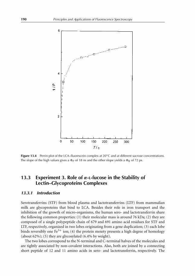
190 Principles and Applications of Fluorescence Spectroscopy
Figure 13.4 Perrin plot of the LCA–fluorescein complex at 20◦C and at different sucrose concentrations.The slope of the high values gives a P of 18 ns and the other slope yields a R of 72 ps.
13.3 Experiment 3. Role of α-L-fucose in the Stability ofLectin–Glycoproteins Complexes
13.3.1 Introduction
Serotransferrins (STF) from blood plasma and lactotransferrins (LTF) from mammalianmilk are glycoproteins that bind to LCA. Besides their role in iron transport and theinhibition of the growth of micro-organisms, the human sero- and lactotransferrin sharethe following common properties: (1) their molecular mass is around 76 kDa; (2) they arecomposed of a single polypeptide chain of 679 and 691 amino acid residues for STF andLTF, respectively, organized in two lobes originating from a gene duplication; (3) each lobebinds reversibly one Fe3+ ion; (4) the protein moiety presents a high degree of homology(about 62%); (5) they are glycosylated (6.4% by weight).
The two lobes correspond to the N-terminal and C-terminal halves of the molecules andare tightly associated by non-covalent interactions. Also, both are joined by a connectingshort peptide of 12 and 11 amino acids in sero- and lactotransferrin, respectively. The

Lens culinaris Agglutinin 191
three-dimensional pictures of the two proteins are perfectly superimposable, with very fewdifferences.
Human STF contains two carbohydrates of the N -acetyllactosaminic type, located in theC-terminal lobe of the polypeptide chain. The two glycosylation sites (Asn-413 and 611)may be occupied by bi-, tri-, and tetra-antennary carbohydrates.
Carbohydrates of human LTF are located in both N- and C-domains, at threeglycosylation sites (Asn-137, 478 and 624).
Carbohydrates of human STF are not fucosylated, while those of human LTF have anα-l,6-fucose bound to the N -acetyl glucosamine residue linked to the peptide chain, andan α-l,3-fucose bound to the N -acetyllactosamine residues.
Studies have shown that the α-l,3-fucose residue does not play any role in the interactionbetween LCA and glycopeptides isolated from human LTF or chemically synthesized(Kornfeld et al. 1981). However, the same work showed that α-l,6-fucose is importantfor a tight binding. Also, X-ray diffraction studies have proved that the α-1,6 fucose isessential for attaining the proper binding conformation of the carbohydrates (Bourne et al.1993).
13.3.2 Binding studies
The goal of these studies is to measure the association constants of the LTF–LCA and STF–LCA complexes. LCA is given as a fluorescein–LCA complex (from Sigma). The extinctioncoefficient of the complex is 132.996 mM−1 cm−1 at 495 nm. Two molecules of fluoresceinare bound to one molecule of LCA. Binding of the STF or LTF to LCA–fluorescein complexinduces a variation in the fluorescence intensity of the extrinsic probe. LTF and STFconcentrations can be determined spectrophotometrically at 280 nm with an absorptionE1% = 14.3 and 14.0, respectively.
Prepare stock solutions of LTF and STF equal to 28 μM.
a Prepare in a fluorescence cuvette around 0.8 μM of LCA–fluorescein solution in PBSbuffer (final volume equal to 1 ml). Then, plot the fluorescence emission spectrum from500 to 560 nm, λex = 495.
Add 5 μl aliquots of LTF or STF solution to the fluorescence cuvette and mix slowly.Then, plot the fluorescence emission spectrum from 500 to 560 nm.
Continue the experiments by adding 10 aliquots of 5 μl each of the LTF or STFsolution.
Repeat each experiment twice.How does the emission intensity of the LCA–fluorescein complex vary with the
addition of LTF or STF? Explain.b Why do we need to use an extrinsic probe to perform our experiments instead of adding
LTF or STF to LCA and following the fluorescence intensity variation of Trp residuesof LCA?
c Measure the intensity of each spectrum at the peak (515 nm) and correct it for thedilution. Then, plot the corrected volume as a function of STF or LTF concentration.
From the shape of the plots drawn, what can you say about the affinities of thetransferrins to LCA?
192 Principles and Applications of Fluorescence Spectroscopy
d The dissociation constants can be calculated using the following equation:
�F/F = (�Fmax/F)(Lb/P) (13.1)
where �F , �Fmax, F , Lb, and P are the fluorescence change for a concentration L of theglycoprotein, the maximum fluorescence change at saturation of the protein with theglycoprotein, the fluorescence intensity of LCA–FITC in the absence of glycoprotein,the concentration of bound glycoprotein, and the total concentration of LCA–FITC,respectively. The concentration of bound glycoprotein can be calculated from the rootof the quadratic equation [Equation (13.2)] arising from the definition of the bindingconstant:
Lb = 0.5{(P0 + L0 + Kd) − [(P0 + L0 + Kd)2 − 4P0L0]1/2} (13.2)
where P0 is the protein concentration.Replacing Equation (13.2) in Equation (13.1) gives Equation (3):
�F/F = (�Fmax/F)×{(P0 + L0 + Kd +[(P0 + L0 + Kd)2 − 4PL]1/2}/2P0 (13.3)
�Fmax can be obtained by plotting 1/�F as a function of 1/L0.From the two plots you obtain, is it possible to determine �Fmax for both LCA–LTF
and LCA–STF interactions? Explain.Note: the whole demonstration of Equation (13.3) is given in Chapter 15.
e After you have determined �Fmax, find the value of the dissociation constants byapplying Equation (13.3). You can do this manually by choosing two to three valuesof �F and L0. For each set of �F and L0, you will have a value for Kd; then you calculatethe mean value of Kd. What is your conclusion concerning the affinities?
f Calculate the values of the affinity constants with Equation (10.22). Do you find thesame values as those obtained with Equation (13.3). Can you explain?
13.3.3 Results
a How does the emission intensity of the LCA–fluorescein complex vary with the additionof LTF or STF? Explain.
Here,we are studying the interaction between two proteins,LCA and LTF or STF,usingfluorescein as a probe. Fluorescein is bound covalently to LCA, and so its fluorescence issensitive to interactions occurring between the proteins. Since we are following bindingexperiments, we have static quenching inducing a decrease in fluorescence intensity offluorescein (Figure 13.5). There is no need for LTF to STF bind to the fluorescein toobserve a decrease in the fluorescence intensity of fluorescein. The external probe ispart of LCA, and so its fluorescence is sensitive to structural modification(s) occurringin LCA.
The emission peak of fluorescein is still in the same position at all LTF concentrations.The reason for this is that the environment of the fluorescein on LCA was not affectedor modified with binding of LTF on LCA. However, it is important to note that thefluorescence emission peak of fluorescein is not very sensitive to all modificationsoccurring in its proximity. Other probes have a much more sensitive emission peak than

Lens culinaris Agglutinin 193
Figure 13.5 Fluorescence spectra of LCA–fluorescein in the absence (a) and presence of increasingconcentrations of LTF. Spectrum j corresponds to 1.223 μM of LTF. λex = 495 nm.
that of fluorescein, which is why it is very important not to generalize the fluorescenceproperties to all fluorophores.
b Why do we need to use an extrinsic probe to perform our experiments instead of addingLTF or STF to LCA and following the fluorescence intensity variation of Trp residuesof LCA?
The three proteins show intrinsic fluorescence due to the presence of Trp residues.Thus, although binding occurs between LCA and LTF or STF, we cannot use fluorescenceof Trp residues of LCA to follow this interaction, since there will be an overlapping withthe fluorescence of Trp residues of LTF or STF. Therefore, it is necessary to use anextrinsic probe, which is bound to one protein only. A covalently bound fluorophoresuch as fluorescein is very suitable to perform binding experiments, since there will beno real binding between the fluorophore and the added protein.
c Figure 13.6 shows the fluorescence intensity at 515 nm of fluorescein bound to LCA inthe presence of increasing concentrations of LTF or STF.
The plots clearly indicate that the affinity of LTF to LCA is much higher than theaffinity of STF to LCA. In fact, the curvature observed for the LTF–STF interaction
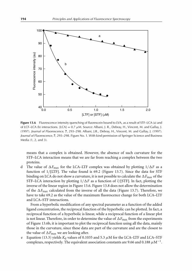
194 Principles and Applications of Fluorescence Spectroscopy
100
90
80
70
Flu
ores
cenc
e in
tens
ity (
au)
60
50
400.0 0.5 1.0
[LTF] or [STF] (�M)
1.5 2.0
b
a
Figure 13.6 Fluorescence intensity quenching of fluorescein bound to LVA, as a result of STF–LCA (a) andof LCF–LCA (b) interactions. [LCA] = 0.7 μM. Source: Albani, J. R., Debray, H., Vincent, M. and Gallay, J.(1997). Journal of Fluorescence, 7, 293–298. Albani, J.R., Debray, H., Vincent, M. and Gallay, J. (1997).Journal of Fluorescence, 7, 293–298. Figure No. 1.With kind permission of Springer Science and BusinessMedia (1, 2, and 3).
means that a complex is obtained. However, the absence of such curvature for theSTF–LCA interaction means that we are far from reaching a complex between the twoproteins.
d The value of �Fmax for the LCA–LTF complex was obtained by plotting 1/�F as afunction of 1/[LTF]. The value found is 69.2 (Figure 13.7). Since the data for STFbinding on LCA do not show a curvature, it is not possible to calculate the �Fmax of theSTF–LCA interaction by plotting 1/�F as a function of l/[STF]. ln fact, plotting theinverse of the linear region in Figure 13.6. Figure 13.8 does not allow the determinationof the �Fmax calculated from the inverse of all the data (Figure 13.7). Therefore, wehave to take 69.2 as the value of the maximum fluorescence change for both LCA–LTFand LCA–STF interactions.
From a hyperbolic modification of any spectral parameter as a function of the addedligand concentration, the reciprocal function of the hyperbolic can be plotted. In fact, areciprocal function of a hyperbolic is linear, while a reciprocal function of a linear plotis not linear. Therefore, in order to determine the value of �Fmax from the experimentsof Figure 13.6b, it is important to plot the reciprocal function using all the data, mainlythose in the curvature, since these data are part of the curvature and are the closest tothe value of �Fmax we are looking after.
e Equation (13.3) yields Kd values of 0.1035 and 5.3 μM for the LCA–LTF and LCA–STFcomplexes, respectively. The equivalent association constants are 9.66 and 0.188 μM−1.

Lens culinaris Agglutinin 195
Figure 13.7 Double reciprocal plot of the LCA–FITC–LTF fluorescence intensity variation vs LTFconcentration.
Figure 13.8 Double-reciprocal plot of the LCA–FITC–LTF fluorescence intensity variation vs LTFconcentration. The data are obtained from the linear part (low concentrations of LTF) of the graph ofFigure 13.6b.
Thus, LTF has its affinity 50 times higher to LCA than STF. The reason for this is thepresence of α-l,6-fucose bound to the N-acetylglucosamine residue.
f Plotting Io/I vs [STF] or [LTF] yields linear graphs with slopes equal to the asociationconstants of the complexes (not shown). The values of Kd were found to be 0.875and 10 μM for the LCA–LTF and LCA–STF complexes, respectively. These values show

196 Principles and Applications of Fluorescence Spectroscopy
that the affinity of LCA to LTF is 11 times higher than that of LCA for STF, and not50 times as we found with Equation (13.3). One reason for this difference is the factthat Equation (10.22) does not take into consideration the concentration of nonboundSTF or LTF.
References
Albani, J.R., Debray, H., Vincent, M. and Gallay, J. (1997). Role of the carbohydrate moiety and of thealpha l-fucose in the stabilization and the dynamics of the Lens culinaris agglutinin–glycoproteincomplex. A fluorescence study. Journal of Fluorescence, 7, 293–298.
Bourne, Y., Van Tilbeurgh, H. and Cambillau, C. (1993). Protein–carbohydrate interactions. CurrentOpinion in Structural Biology, 3, 681–686.
Kornfeld, K., Reitman, M.-L. and Kornfeld, R. (1981). The carbohydrate-binding specificity of pea andlentil lectins. Fucose is an important determinant. Journal of Biological Chemistry, 256, 6633–6640.
Tuma, J.J. (1983). Handbook of Physical Calculations, McGraw-Hill, New York.

Chapter 14
Förster Energy Transfer
14.1 Principles and Applications
Förster energy transfer or energy transfer at a distance occurs between two molecules,a donor (the excited fluorophore) and an acceptor (a chromophore or a fluorophore)(Forster 1948). Energy is transferred by resonance, i.e., the electron of the excited moleculeinduces an oscillating electric field that excites acceptor electrons. The latters will reach anexcited state. If the acceptor is fluorescent, its de-excitation will occur mainly by a photonemission. However, if it does not fluoresce, it will return to a fundamental state as a resultof its interaction with the solvent. Energy-transfer efficiency depends on three parameters,distance R between the donor and acceptor, spectral overlap between the donor fluorescencespectrum and the acceptor absorption spectrum (Figure 14.1), and the orientation factor κ2,which gives an indication of the relative alignment of the dipoles of the acceptor in thefundamental state and of the donor in the excited state.
The distance that separates the two molecules goes from 10 to 60–100 Å. Below 10 Å,electron transfer may occur between the two molecules, inducing an energy transfer fromdonor to acceptor. κ2 values hold from 0 to 4. For aligned and parallel transition dipoles(maximal energy transfer) κ2 is 4, and if the dipoles are oriented perpendicular to eachother (very weak energy transfer), κ2 is 0. When κ2 is not known, its value is considered tobe equal to 2/3. This value corresponds to a random relative orientation of the dipoles.
The energy-transfer mechanism can be described by the following:
D + hνo → D∗ absorption
D∗ → D + hν1 fluorescence
D∗ → D nonradiative de-excitation
D∗ + A → D + A∗ energy transfer
A∗ → A nonradiative de-excitation
A∗ → A + hν2 induced fluorescence
Figure 14.2 shows fluorescence intensity quenching of 4′,6-diamidino-2-phenylindole(DAPI) complexed to DNA in the presence of two concentrations of Acridine Orange.In fact, one can see that while the fluorescence intensity of DAPI decreases, that of Acridine

198 Principles and Applications of Fluorescence Spectroscopy
550500
Wavelength (nm)
121.0
0.5
450400
Figure 14.1 Normalized corrected emission spectrum of apoHb–ANS complex upon excitation at350 nm. 2: Normalized absorption spectrum of apo FIA. Reprinted with permission from Sassaroli, M.,Bucci, E., Liesegang, J., Fronticelli, C. and Steiner, R. F. (1984). Biochemistry, 2487–2491. Copyright ©1984 American Chemical Society.
550500
Wavelength (nm)
DAPIAO
0.03
0
0.045 bp−1
Flu
ores
cenc
e in
tens
ity
450400
Figure 14.2 Fluorescence emission spectra of DNA-bound DAPI in the presence of 0.03 and 0.045 bp−1
of AO. The excitation wavelength is 360 nm. Source: Maliwal, B.P., Kusba, J. and Lakowicz, J.R. (1995).Biopolymers, 35, 245–255. Reprinted with permission from John Wiley & Sons, Inc.
Orange increases. This type of experiment is one of several ways to show the presence ofthe energy-transfer mechanism.
Also, one can put into evidence the energy-transfer mechanism by recording thefluorescence excitation spectrum of the complex (donor–acceptor) (λem is set at awavelength where only the acceptor emits) and comparing it to the absorption spectrumof the donor alone. In the presence of energy transfer between the two molecules, a peakcharacteristic of the donor absorption will be displayed in the fluorescence excitationspectrum.

Förster Energy Transfer 199
Membranes fusion can be studied using the energy-transfer mechanism. In fact,membrane vesicles labeled with both NBD and rhodamine probes are fused with unlabeledvesicles. In the labeled vesicles, upon excitation of NBD at 470 nm, emission from rhodamineis observed at 585 nm as a result of energy transfer from NBD to rhodamine. The averagedistance separating the donor from the acceptor molecules increases with fusion of thevesicules, thereby decreasing the energy-transfer efficiency (Struck et al. 1981).
Energy transfer is considered as a type of dynamic quenching. In general, dynamicquenching can be described with three different processes: electron transfer, electronexchange, and Förster or coulombic energy transfer (Figure 14.3).
D*
D+ •A−
D+ •A−
D−
•A
D •A*
D* •A
D* •A
D* •A
D* •A
D •A*
D •A*
1
or
2
Radical ion pair
Electron transfer
Electron exchange
Dipole–dipole coupling
•A+
Figure 14.3 Different mechanisms of dynamic quenching.

200 Principles and Applications of Fluorescence Spectroscopy
Electron exchange and coulombic modes are part of what we can call in general theenergy-transfer mechanism. In the coulombic mode, an electron transfer does not occurbetween donor and acceptor molecules, but two transitions are observed simultaneously.The rate of dipole–dipole transfer depends on the oscillator strength of the radiativetransitions, which is not the case for the electron-exchange mechanism. Also, in the Förstermechanism, there is a dipole–dipole coupling mechanism, which is effective in the singlet–singlet energy transfer only, as a result of the large transition dipoles. Finally, both Försterand electron-exchange rate constants depend on the spectral overlap integral J between theemission spectrum of the donor and the absorption spectrum of the acceptor. A high valueof J induces a high electron rate.
Combination of time-resolved fluorescence and Förster energy transfer was applied
in the method known as HTRF® (homogeneous time-resolved fluorescence) developedby Cisbio (http://www.htrf-assays.com/). This allows the use of a lanthanide, such aseuropium, with an extremely long emission half-life (from μs to ms) and a large Stokesshift, compared to more traditional fluorophores. Conjugation of Eu3+ to cryptategives an entity which confers increased assay stability and the use of a patentedratiometric measurement that allows correction for quenching and sample interferences.This powerful combination provides significant benefits to drug-discovery researchersincluding assay flexibility, reliability, increased assay sensitivity, higher throughput, andfewer false-positive/false-negative results.
Many compounds and proteins present in biological fluids or serum are naturallyfluorescent, and the use of conventional, prompt fluorophores leads to serious limitations inassay sensitivity. The use of long-lived fluorophores combined with time-resolved detection(a delay between excitation and emission detection) minimizes any prompt fluorescenceinterference. However, it is difficult to generate fluorescence of lanthanide ions by directexcitation, because of the ions’ poor ability to absorb light. Lanthanides must first becomplexed with organic moieties that harvest light and transfer it to the lanthanide throughintramolecular, nonradiative processes. Rare earth chelates and cryptates are examples oflight-harvesting devices. The collected energy is transferred to the rare earth ion, whichthen emits its characteristic long-lived fluorescence.
To be successfully used as labels in biological assays, rare earth complexes shouldpossess specific properties including stability, high light yield, and ability to be linked tobiomolecules. Moreover, insensitivity to fluorescence quenching is of crucial importancewhen working directly in biological fluids. When complexed with cryptates, however, manyof these limitations are eliminated.
In HTRF®, the donor is europium cryptate, which has the long-lived emissions oflanthanides coupled with the stability of cryptate encapsulation, and the primary acceptorfluorophore is XL665, a modified allophycocyanin. When these two fluorophores arebrought together by a biomolecular interaction and after excitation, some of the energycaptured by the Cryptate is released through fluorescence emission with a peak at 620 nm,while the remaining energy is transfered to XL665. This energy is then released by XL665as specific fluorescence at 665 nm. Emission at 665 nm occurs only through FRET witheuropium. Because europium cryptate is always present in the assay, light at 620 nmis detected even when the biomolecular interaction does not bring XL665 within closeproximity.

Förster Energy Transfer 201
HTRF® is a highly flexible chemistry and has been successfully used to measure molecularcomplexes of many different sizes. This includes assessment of small phosphorylatedpeptides, immunoassays for quantifying large glycoproteins such as thyroglobulin, receptortyrosine kinase activity using membrane preparations, and indirect detection (via secondaryantibodies) of tagged complexes such as CD28/CD86 binding.
Heparanase, a heparan sulfate-specific endo-β-d-glucuronidase, cleaves heparin sulfate(HS) into characteristic large-molecular-weight fragments. HS degradation causes therelease of angiogenic and growth factors which lead to tumor-cell proliferation andmigration, and to angiogenesis. Heparanase is therefore an attractive target for thedevelopment of new anti-metastatic therapeutics. Chikachi et al. developed a highlysensitive, quantitative, and robust heparanase assay using HTRF® technology and basedon time-resolved fluorescence energy transfer (TR-FRET) between europium cryptate andXL665 (allophycocyanin) (Figure 14.4).
Cryptates are formed by the inclusion of a cation into a tridimensional cavity. Theproperties of the trisbypyridine macrocycle, for instance (Figure 14.5), favor such a tight
FRET
337 nmexcitation
665 nmemission
Biotinylated-HS-Eu(K)
Heparanase
StreptavidinXL665
Figure 14.4 Heparanase assay configuration. Courtesy of Cisbio.
CO2H
CO2HHO2C
HO2C
HO2CN N
NN
N
N N
R
N
Eu3+
Figure 14.5 Structure of trisbypirydine pentacarboxylate Eu3+ cryptate. Courtesy of Cisbio.

202 Principles and Applications of Fluorescence Spectroscopy
0.0001
1800
1600
ΔF %
1400
1200
1000
800
600
4000.001 0.01 0.1 1 10 100
Protein (�g ml−1)
Figure 14.6 Heparanase activity titration curve.
association of the cage with the europium in that this interaction becomes virtuallyunchallengeable, and leads to an exceptionally inert complex.
The classical TBP Eu3+ has its excitation peak at 307 nm and, substituting carboxylicgroups on two of the bipyridine units, leads to a shift in the excitation peak to 325 nm. Thus,excitation with a nitrogen laser at 337 nm induces an increase in the cryptate fluorescenceby 2.5. Energy transfer was observed when an HS substrate labeled with cryptate andbiotin were incubated with streptavidin-XL665. In this assay configuration, the maximumsignal was obtained without enzymes. Cleavage of the biotin-HS-cryptate substrateby heparanase prevented FRET from occurring and therefore led to a signal decrease(Figure 14.6).
14.2 Energy-transfer Parameters
Let us consider kt as the rate constant of the excited state depopulation via the energy-transfer mechanism; the measured fluorescence lifetime is thus equal to
1
τt= 1
τo+ kt (14.1)
where l/τ is the de-excitation rate constant in the absence of energy transfer. The efficiencyE of de-excitation by means of the energy-transfer mechanism is
E = kt
kt + 1/τo= 1/τt − 1/τo
1/τt= 1 − 1/τo
1/τt= 1 − τt
τo(14.2)
The energy-transfer mechanism appears to affect the fluorescence lifetime, intensity, andquantum yield:
E = 1 − I
Io= 1 − φt
φo= 1 − τt
τo(14.3)
where τ , I , and φt are the mean fluorescence lifetime and intensity in the absence (τo, Io,and φo) and presence of the quencher (τt, I , and φt).

Förster Energy Transfer 203
The distance R that separates the donor from the acceptor is calculated usingEquation (14.4):
R = R0
(1 − E
E
)1/6
(14.4)
The Förster distance Ro(Å) at which the energy-transfer efficiency is 50% is calculated usingEquation (14.5):
R0 = 9.78 × 10³[κ2n−4QDJ (λ)]1/6 (14.5)
where κ2 is the orientation factor (=2/3), n the refractive index (=1.33) and QD the averagequantum yield of the donor in the absence of the acceptor.
From the overlap of the emissium spectrum of the donor and the absorption spectrumof the acceptor, we can calculate the overlap integral J (M−1cm3))
J (λ) =∫ ∞
0 FD(λ) · εA(λ) · λ4 dλ∫ ∞0 FD(λ) dλ
(14.6)
εA is the extinction coefficient of the acceptor expressed in M−1cm−1, FD the fluorescenceintensity of the donor expressed in arbitrary units, and λ the wavelength (cm).
The distance R that separates the donor from the acceptor can be determined fromX-ray diffraction studies. The κ2 value of the five tryptophan residues of cytochromeP-450 has been determined. Cytochrome P-450, a superfamily of heme proteins, catalysesmonooxygenation of a wide variety of hydrophobic substances of xenobiotic and exogenousorigin (Guengerich 1991; Porter and Coon 1991). Cytochrome P-450 from Bacillusmegaterium strain ATCC 14581 called cytochrome P-450BM3 is a monomer of molecularmass of 119 kDa, comprising an N-terminal P-450 heme domain linked to a C-terminalreductase domain (Narhi and Fulco 1986). The heme domain of cytochrome P-450BM3
contains five tryptophan residues (Figure 14.7). The distances of the tryptophans from
N-terminus90
96
Heme
367325
130
C-terminus
Figure 14.7 Location of five tryptophan residues (shown in a ball-and-stick representation) and the hemeprosthetic group (white ball and stick) in the heme domain of cytochrome P-450BM3.

204 Principles and Applications of Fluorescence Spectroscopy
20
W96
T2
T1D
ista
nce
of T
rp fr
om h
eme
(nm
)
W367
W130
W325W90
10
0 1 2
k 2
3 4
Figure 14.8 Plot of κ2 against the distance of tryptophan residues from the heme in cytochrome P-450. The dotted lines in the figure show the crystallographic distances between tryptophan residues, andlines labeled with τx and τ2 show the calculated distances between the heme and different tryptophanresidues using all possible values of κ2 (0.0–4.0). The point where these two lines intersect shows the κ2
value for the particular residue and is indicated by the arrows. Source of figures 11.22 and 11.23: Khan,K.K., Mazumdar, S., Modi, S., Sutcliffe, M., Roberts, G.C.K. and Mitra, S. (1997). European Journal ofBiochemistry, 244, 361–370.
the heme are 1.224 (Trp96), 1.834 (Trp90), 1.85 (Trp325), 1.968 (Trp367), and 2.365 nm(Trp130). Fluorescence intensity decay yields three fluorescence lifetimes equal to 0.2, 1,and 5.4 ns with fractional contributions of 61%, 33%, and 6%, respectively.
Figure 14.8 shows the plot of Trp to heme distance obtained by fluorescence energytransfer as a function of κ2 (from 0 to 4) for the two shortest fluorescence lifetimes (solidcurve). The five dotted lines in the figure show the crystallographic distances betweentryptophan residues and heme. The intersection between the crystallographic lines and theenergy-transfer plots is equal to the κ2 corresponding to the specific tryptophan.
14.3 Bioluminescence Resonance Energy Transfer
Bioluminescence resonance energy transfer (BRET) takes advantage of the Förster resonanceenergy transfer and is observed in the sea pansy Renilla reniformis. This organism expressesa luciferase, which emits blue light when it is purified. If the luciferase is excited in intactcells, green light occurs, because in vivo the luciferase is associated with the green fluorescentprotein (GFP), which accepts the energy from the luciferase and emits green light. BREToccurs in the 1–10 nm regions, which is comparable with the dimensions of biologicalmacromolecules and makes it an ideal system for the study of protein–protein interactionin living cells (Ayoub et al. 2002).
Green fluorescent protein is commonly used for energy-transfer experiments (Baubetet al. 2000). The fluorescent moiety of GFP protein is the Ser–Tyr–Gly derived chromophore.GFP can be expressed in a variety of cells where it becomes fluorescent, can be fused to a host

Förster Energy Transfer 205
protein, and can be mutated so that the mutants have different fluorescence properties andcan be used in energy-transfer studies. Some examples, the blue fluorescent protein (BFP),which is a GFP mutant with a Tyr66His mutation, absorbs at 383 nm and emits at 447 nm.In energy-transfer experiments, BFP is a donor molecule to GFP. In a system with randomlyoriented chromophores, the distance Ro at which 50% energy transfer occurs is found to beequal to 4 nm (Heim 1999). Cyan fluorescent protein (CFP) contains a Tyr66Trp mutationand absorbs and emits at 436 and 476 nm, respectively. Yellow fluorescent protein (YFP) is aThr203Tyr mutant with excitation and emission peaks equal to 516 and 529 nm, respectively.In the CFP–YFP pair, CFP is the donor molecule, and the YFP is the acceptor molecule.The value of Ro found for randomly oriented chromophores is 5.2 nm. The CFP–YFP pairfused to proteins has been used in resonance energy-transfer studies along with multifocalmultiphoton microscopy to measure transport phenomena in living cells (Majoul et al.2002) and protein–protein interaction and structural changes within a molecule (Truongand Ikura 2001).
Also, the Phe-64 → Leu and Ser-65 → Thr mutant shows higher fluorescence parametersthan that of the wild GFP. Excitation at 458 nm yields a fluorescence spectrum with twopeaks at 512 and 530 nm. The fluorescence properties of this enhanced green fluorescentprotein (EGFP) were found to be similar to the recombinant glutathione S-transferase–EGFP (GST–EGFP) protein, expressed in Escherichia coli (Cinelli et al. 2004).
Imaging fluorescence resonance energy-transfer studies between two GFP mutants inliving yeast have also been performed. The donor was the GFP mutant P4.3, bearing theY66H and Y145F mutations, and the acceptor was the GFP mutant S65T (Sagot et al. 1999).The authors constructed a concatemer where the two GFP mutants were linked by a spacercontaining a protease-specific recognition site. The tobacco etch virus (TEV) protease wasadded to cleave the covalent bond between the two fluorophores. Experiments performedin vitro show that excitation of the donor at 385 nm leads to the emission of both the donorand the acceptor at emission peaks equal to 385 and 445 nm, respectively. Addition of TEVprotease induces an increase in the donor emission and a decrease of the emission acceptor.Experiments performed in vivo reveal that in the presence of protease, the energy-transferloss is around 57%.
In most BRET applications, the fused donor is Renillaluciferase (Rluc) rather thanaequorin, to avoid any intrinsic affinity for Aequorea-derived GFP mutant; the acceptoris the YFP, to increase the spectral distinction between the two emissions. When the donorand acceptor are in close proximity, the energy resulting from catalytic degradation of thecoelenterazine derivative substrate is transferred from the luciferase to the YFP, which willthen emit fluorescence at its characteristic wavelength (Xu et al. 1999).
To demonstrate the clear discrimination between positive and negative control ofthe BRET assay technology, the luminescence and fluorescence signals of theBRET2™ demo kit (Perkin Elmer Life Sciences) were quantified on the microplatereader POLARstar OPTIMA (BMG Labtech: http://www.pharmaceutical-technology.com/contractors/lab_equip/bmg_labtech/), allowing the monitoring of the kinetic curves andthe calculation of the BRET ratio. The BRET2™ demo kit applies the cell-permeable andnontoxic coelenterazine derivative substrate DeepBlueC™ (DBC) and a mutant of theGFP2 as acceptor. These compounds show improved spectral resolution and sensitivityover earlier variants. Four sets of samples were run in triplicate, a blank (non-transfectedcells), a positive control (Rluc-GFP2), a negative control (Rluc + GFP2), and a buffer control
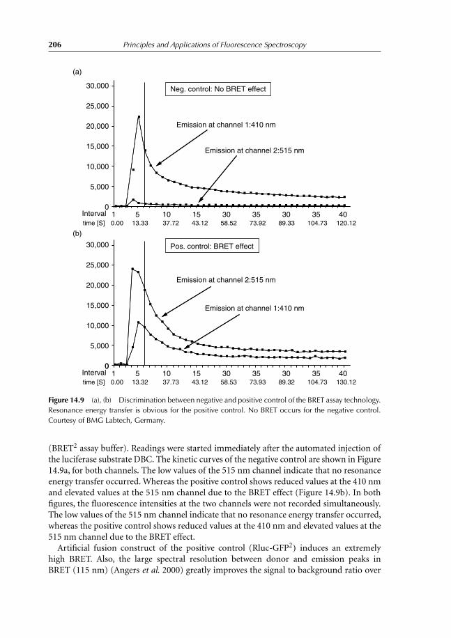
206 Principles and Applications of Fluorescence Spectroscopy
30,000
25,000
Pos. control: BRET effect
Emission at channel 1:410 nm
20,000
15,000
10,000
5,000
01Interval
time [S] 0.00 13.32 37.73 43.12 58.53 73.93 89.32 104.73 130.125 10 15 30 35 30 35 40
0
30,000
(a)
(b)
25,000
Neg. control: No BRET effect
Emission at channel 1:410 nm
Emission at channel 2:515 nm
20,000
15,000
10,000
5,000
01Interval
time [S] 0.00 13.33 37.72 43.12 58.52 73.92 89.33 104.73 120.125 10 15 30 35 30 35 40
Emission at channel 2:515 nm
Figure 14.9 (a), (b) Discrimination between negative and positive control of the BRET assay technology.Resonance energy transfer is obvious for the positive control. No BRET occurs for the negative control.Courtesy of BMG Labtech, Germany.
(BRET2 assay buffer). Readings were started immediately after the automated injection ofthe luciferase substrate DBC. The kinetic curves of the negative control are shown in Figure14.9a, for both channels. The low values of the 515 nm channel indicate that no resonanceenergy transfer occurred. Whereas the positive control shows reduced values at the 410 nmand elevated values at the 515 nm channel due to the BRET effect (Figure 14.9b). In bothfigures, the fluorescence intensities at the two channels were not recorded simultaneously.The low values of the 515 nm channel indicate that no resonance energy transfer occurred,whereas the positive control shows reduced values at the 410 nm and elevated values at the515 nm channel due to the BRET effect.
Artificial fusion construct of the positive control (Rluc-GFP2) induces an extremelyhigh BRET. Also, the large spectral resolution between donor and emission peaks inBRET (115 nm) (Angers et al. 2000) greatly improves the signal to background ratio over
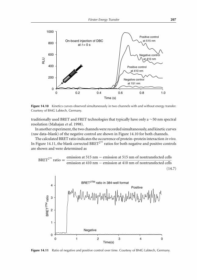
Förster Energy Transfer 207
1000
800
600
400
200
00 0.2 0.4 0.6
Time (s)
0.8 1.0
RLU
On-board injection of DBCat t = 0 s
Positive controlat 515 nm
Negative controlat 410 nm
Negative controlat 151 nm
Positive controlat 410 nm
Figure 14.10 Kinetics curves observed simultaneously in two channels with and without energy transfer.Courtesy of BMG Labtech, Germany.
traditionally used BRET and FRET technologies that typically have only a ∼50 nm spectralresolution (Mahajan et al. 1998).
In another experiment, the two channels were recorded simultaneously, and kinetic curves(raw data–blank) of the negative control are shown in Figure 14.10 for both channels.
The calculated BRET ratio indicates the occurrence of protein–protein interaction in vivo.In Figure 14.11, the blank corrected BRET2™ ratios for both negative and positive controlsare shown and were determined as
BRET2™ ratio = emission at 515 nm − emission at 515 nm of nontransfected cells
emission at 410 nm − emission at 410 nm of nontransfected cells
(14.7)
4
3
2
1
00 1 2 3
Time(s)4 0
PositiveBRET2TM ratio in 384-well format
BR
ET
2TM
rat
io
Negative
Figure 14.11 Ratio of negative and positive control over time. Courtesy of BMG Labtech, Germany.

208 Principles and Applications of Fluorescence Spectroscopy
The signal for negative and positive control here reveals a value of around 0.06 and 3.3,respectively, which leads to a factor of around 50 and a clear discrimination between thesecontrols. The high factor between these controls is caused by the artificial fusion constructof the positive control (Rluc-GFP2) resulting in an extremely high BRET.
The main disadvantages of FRET, as opposed to BRET, are the consequences of therequired excitation of the donor with an external light source. BRET assays show no photo-bleaching or photo-isomerization of the donor protein, no photo-damage to cells, andno light scattering or autofluorescence from cells or microplates, which can be caused byincident excitation light. In addition, one main advantage of BRET over FRET is the lackof emission arising from direct excitation of the acceptor. This reduction in backgroundshould permit detection of interacting proteins at much lower concentrations than ispossible for FRET. However, BRET requires the addition of a cofactor, and for someapplications, e.g., determining the compartmentalization and functional organization ofliving cells, the GFP-based FRET method is superior to BRET due to the much higher lightoutput.
In conclusion, BRET offers the ability to directly study complex protein–proteininteractions in living cells. There is no need for an excitation light source. Therefore,photosensitive tissue can be used for BRET, and problems associated with FRET-basedassays such as photo-bleaching, autofluorescence, and direct excitation of the acceptor areeliminated.
References
Angers, S., Salahpour,A., Joly, E., Hilairet, S., Chelsky, D., Dennis, M. and Bouvier, M. (2000). Detectionof b2-adrenergic receptors dimerization in living cells using bioluminescence resonance energytransfer (BRET). Proceedings of the National Academy of Sciences, USA, 97, 3684–3689.
Ayoub, M.A., Couturier, C., Lucas-Meunier, E., Angers, S., Fossier, P., Bouvier, M. and Jockers, R.(2002). Monitoring of ligand-independent dimerization and ligand-induced conformationalchanges of melatonin receptors in living cells by bioluminescence resonance energy transfer.Journal of Biological Chemistry, 277, 21522–21528.
Baubet, V., Le Mouellic, H., Campbell, A.K., Lucas-Meunier, E., Fossier, P. and Brûlet, P. (2000).Chimeric green fluorescent protein-aequorin as bioluminescent Ca2+ reporters at the single-celllevel. Proceedings of the National Academy of Sciences, USA, 97, 7260–7265.
Cinelli, R.A.G., Ferrari, A., Pellegrini, V., Tyagi, M., Giacca, M. and Beltram, F. (2004). The enhancedgreen fluorescent protein as a tool for the analysis of protein dynamics and localization: Localfluorescence study at the single-molecule level. Photochemistry and Photobiology, 71, 771–776.
Forster, T. (1948). Intermolecular energy migration and fluorescence. Annual of Physics (Leipzig), 2,55–75.
Guengerich, F.P. (1991). Reactions and significance of cytochrome P-450 enzymes. Journal of BiologicalChemistry, 266, 10019–10022.
Heim, R. (1999). Green fluorescent protein forms for energy transfer. Methods in Enzymology, 302,408–423.
Khan, M.J., Joginadha Swamy, M., Krishna Sastry, M.V., Umadevi Sajjan, S., Patanjali, S.R., Rao, P.,Swarnalatha, G.V., Banerjee, P. and Surolia, A. (1988). Saccharide binding to three Gal/GalNacspecific lectins: Fluorescence, spectroscopic and stopped-flow kinetic studies. GlycoconjugateJournal, 5, 75–84.
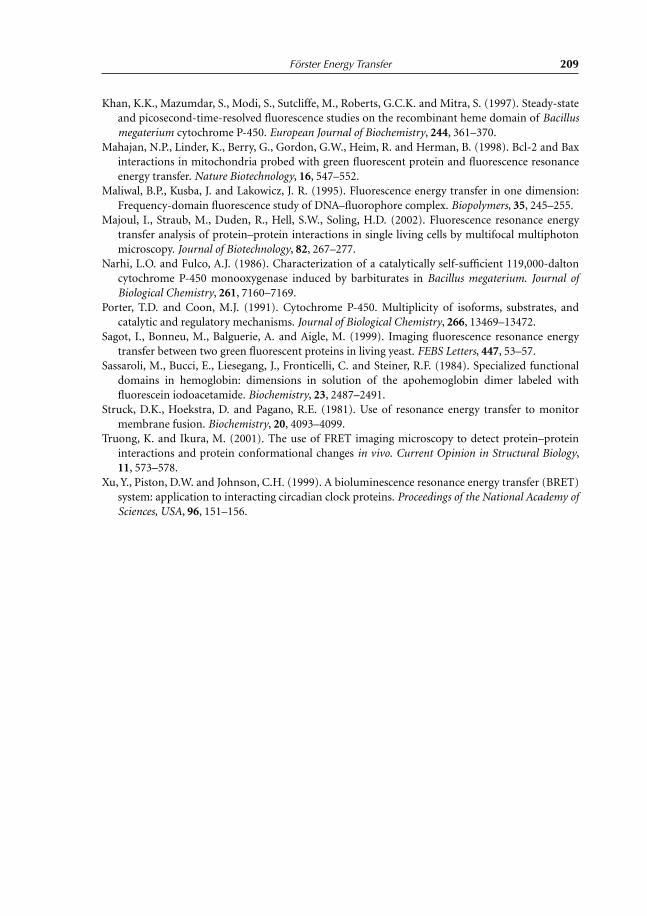
Förster Energy Transfer 209
Khan, K.K., Mazumdar, S., Modi, S., Sutcliffe, M., Roberts, G.C.K. and Mitra, S. (1997). Steady-stateand picosecond-time-resolved fluorescence studies on the recombinant heme domain of Bacillusmegaterium cytochrome P-450. European Journal of Biochemistry, 244, 361–370.
Mahajan, N.P., Linder, K., Berry, G., Gordon, G.W., Heim, R. and Herman, B. (1998). Bcl-2 and Baxinteractions in mitochondria probed with green fluorescent protein and fluorescence resonanceenergy transfer. Nature Biotechnology, 16, 547–552.
Maliwal, B.P., Kusba, J. and Lakowicz, J. R. (1995). Fluorescence energy transfer in one dimension:Frequency-domain fluorescence study of DNA–fluorophore complex. Biopolymers, 35, 245–255.
Majoul, I., Straub, M., Duden, R., Hell, S.W., Soling, H.D. (2002). Fluorescence resonance energytransfer analysis of protein–protein interactions in single living cells by multifocal multiphotonmicroscopy. Journal of Biotechnology, 82, 267–277.
Narhi, L.O. and Fulco, A.J. (1986). Characterization of a catalytically self-sufficient 119,000-daltoncytochrome P-450 monooxygenase induced by barbiturates in Bacillus megaterium. Journal ofBiological Chemistry, 261, 7160–7169.
Porter, T.D. and Coon, M.J. (1991). Cytochrome P-450. Multiplicity of isoforms, substrates, andcatalytic and regulatory mechanisms. Journal of Biological Chemistry, 266, 13469–13472.
Sagot, I., Bonneu, M., Balguerie, A. and Aigle, M. (1999). Imaging fluorescence resonance energytransfer between two green fluorescent proteins in living yeast. FEBS Letters, 447, 53–57.
Sassaroli, M., Bucci, E., Liesegang, J., Fronticelli, C. and Steiner, R.F. (1984). Specialized functionaldomains in hemoglobin: dimensions in solution of the apohemoglobin dimer labeled withfluorescein iodoacetamide. Biochemistry, 23, 2487–2491.
Struck, D.K., Hoekstra, D. and Pagano, R.E. (1981). Use of resonance energy transfer to monitormembrane fusion. Biochemistry, 20, 4093–4099.
Truong, K. and Ikura, M. (2001). The use of FRET imaging microscopy to detect protein–proteininteractions and protein conformational changes in vivo. Current Opinion in Structural Biology,11, 573–578.
Xu, Y., Piston, D.W. and Johnson, C.H. (1999). A bioluminescence resonance energy transfer (BRET)system: application to interacting circadian clock proteins. Proceedings of the National Academy ofSciences, USA, 96, 151–156.
Chapter 15
Binding of TNS on Bovine Serum Albumin atpH 3 and pH 7
15.1 Objectives
The purpose of this experiment is to find out how pH affects proteins tertiary structure andthus the binding of a ligand to proteins. In principle, when a protein is dissolved in a bufferwith a pH far from its physiological pH, its tertiary structure is altered. Therefore, we canspeak of partial or complete denaturation or unfolding of the protein. The characteristics ofan unfolded protein such as ligand binding differ from those of the folded protein. One canfollow the protein–ligand interaction by recording the fluorescence emission parameters(intensity, anisotropy, and lifetime) of the protein Trp residues and of the ligand if it isfluorescing. In the present work, students will study the structural alteration of bovineserum albumin (BSA) with pH, by following the fluorescence of both protein Trp residuesand of TNS.
15.2 Experiments
15.2.1 Fluorescence emission spectra of TNS–BSA at pH 3 and 7
Plot the fluorescence emission spectra from 290 to 500 nm (λex = 280 nm) of 1.5 μM BSAsolutions prepared at pH 3 and 7. Then, to each cuvette, add 15 μM TNS and record theprotein emission spectra at the two pHs. Correct the fluorescence intensity for the innerfilter effect, and then plot the corrected emission spectra. What do you notice? Are thespectra obtained at the two pHs identical? What are the values of the emission peaks youobserve? Explain the results you obtained.
Do not forget to measure the optical densities at the excitation wavelength and along theemission spectra ε of bovine serum albumin at 280 nm is 43 824 M−1 cm−1 and of TNS at317 nm, 1.89 × 10⁴ M−1 cm−1.
15.2.2 Titration of BSA with TNS at pH 3 and 7
To a cuvette containing 1.5–2 μM bovine serum albumin solution, add equal volumes ofTNS solution so that you have 0.3–15 μM TNS in the cuvette. For each TNS concentration

Binding of TNS on Bovine Serum Albumin 211
(0–15 μM), measure the optical densities at 280, 317, and 335 nm, and plot the emissionspectrum from 290 to 500 nm (λex = 280 nm). The experiment should be performed atpHs 3 and 7. What can you say about the variation of the fluorescence emission intensities?Explain the phenomena you are observing. Do you observe an isoemissive point? Explain.
Measure the fluorescence intensities at 335 nm at the different TNS concentrations, andcorrect them first for the dilution then for the inner filter effect. Finally, plot the fluorescenceintensity at 335 nm as a function of TNS concentration. What do you observe?
For each TNS concentration, measure the intensity variation �I , and then plot 1/�I asa function of 1/[TNS]. By extrapolating to 1/[TNS] = 0, we can calculate �Imax. Is �Imax
the same for both pHs? Explain. Determine the apparent value of the association constantKa of the TNS–BSA complex. Are the association constants equal? Explain.
Plot the ratio Io/I vs. [TNS] for each pH and calculate the apparent value of theassociation constant Ka of TNS–BSA complex. Are the association constants calculatedidentical to those obtained by plotting the inverse equation 1/�I vs. 1/[TNS]?
15.2.3 Measurement of energy-transfer efficiency from Trp residues to TNS
From the data obtained in the titration experiments, calculate the energy-transferefficiency, E
E = 1 − I
Io(14.3)
for each TNS concentration, then determine the value of E at infinite concentrations ofTNS by plotting 1/E vs. 1/[TNS] . Is the value of E the same for both pHs? Explain.
15.2.4 Interaction between free Trp in solution and TNS
Repeat the experiment between TNS and BSA by replacing BSA with free L-Trp. What doyou observe? By plotting Io/I vs. [TNS] what is the nature of the constant you will calculate?
15.3 Results
Figure 15.1 shows the fluorescence emission spectrum of BSA Trp residues in the absence(spectrum a) and presence of TNS (b), both recorded at pH 3. First, we see that thefluorescence emission peak (325 nm) of the Trp residues of the protein decreases to almostzero in the presence of TNS, while an important emission peak at 435 nm characterizingthe fluorescence emission of TNS bound to BSA appears.
The decrease in fluorescence intensity of the Trp residues is the result of energy transferthat is occurring from aromatic residues to bound TNS. The fluorescence of the ligandincreases as a result of its binding to BSA and of the energy transfer that is occurring fromTrp residues to TNS.
Figure 15.2 shows fluorescence emission spectra of BSA in the absence (a) and presence(b) of TNS, both recorded at pH 7. The fluorescence emission peak of Trp residues is

212 Principles and Applications of Fluorescence Spectroscopy
Figure 15.1 Fluorescence emission of BSA recorded in the absence (a) and presence of TNS (b) at pH 3.Spectra are corrected for the inner filter effect. λex = 280 nm.
located at 335 nm and is still observed in the presence of TNS. This means that the energytransfer between Trp residues and TNS is less important at pH 7 than at pH 3 and/or theinteraction between TNS and BSA is weaker at pH 7 than at pH 3. We can observe also thatthe decrease in fluorescence intensity of the Trp residues is associated with the increase inthe fluorescence intensity of bound TNS. In fact, for the same concentrations of BSA (2 μM)and of TNS (15 μM), the fluorescence intensity increase in bound TNS is less importantat pH 7 than at pH 3. Thus, one should conclude that the affinity of TNS to the protein atpH 3 is higher than its affinity at pH 7 inducing a better interaction between TNS and BSAat pH 3. Also, one should not rule out the possibility of having more binding sites for TNSon BSA at pH 3 than at pH 7.
Titration of a constant concentration of BSA with TNS yields a decrease in thefluorescence intensity of the Trp residues together with an increase in the fluorescenceintensity of TNS (not shown). We do not observe an isoemissive point at either pH, thusindicating that TNS has more than one binding site on BSA. After correcting the fluorescenceintensities at the emission peak of Trp residues for the dilution and then for the opticaldensities at the excitation (λex = 280 nm) and emission wavelengths (335 or 325 nm),we can plot the fluorescence intensity as a function of TNS concentration at pH 3 and 7(Figure 15.3). Results indicate that the fluorescence-intensity decrease is more important atpH 3 than at pH 7. This means that the interaction between TNS and BSA is more importantat a low pH.
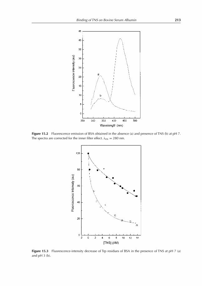
Binding of TNS on Bovine Serum Albumin 213
Figure 15.2 Fluorescence emission of BSA obtained in the absence (a) and presence of TNS (b) at pH 7.The spectra are corrected for the inner filter effect. λex = 280 nm.
Figure 15.3 Fluorescence-intensity decrease of Trp residues of BSA in the presence of TNS at pH 7 (a)and pH 3 (b).

214 Principles and Applications of Fluorescence Spectroscopy
Plotting the variation �I of fluorescence decrease as a function of added TNSconcentration yields a hyperbolic plot at both pHs (Figure 15.4). However, this hyperbolicplot is more obvious at pH 3 than at pH 7. Hyperbolic plots can be described by the followingequation:
�I = �ImaxD
�Imax + Kd(15.1)
where D is the concentration of added TNS, Kd the dissociation constant of TNS–BSAcomplex, and �Imax the maximal variation when TNS binding site on BSA is saturated.
Figure 15.4 Variation of �I with [TNS] at pH 3 and 7.
The inverse plot of a hyperbolic equation is linear, and so the inverse plot ofEquation (15.1) is
1
�I= 1
�Imax+ Kd
�ImaxD(15.2)
Plotting 1/�I vs. 1/[TNS] yields a straight line with a slope equal to Kd/�Imax andintercept equal to 1/�Imax.
Figure 15.5 shows inverse plots obtained at pH 7 and 3. The plots are obtained byusing all the measurements performed. This yields a value of �Imax of 96.52 and 67.52at pH 3 and 7, respectively, with dissociation constants equal to 1.74 and 6.28 μM,respectively.

Binding of TNS on Bovine Serum Albumin 215
Figure 15.5 Double reciprocal plots of the fluorescence-intensity variation vs. [TNS] concentration.
The value of �Imax obtained at pH 7 is lower than the value obtained at the highestconcentration of TNS reached in the experiment. The reason for this is the choice of thedata used to plot Figure 15.5. In fact, we notice that the lowest values of TNS have been takeninto consideration to plot the graph, while the highest values were not. This is a mistake,since the maximum value obtained at saturation is closer to the highest measured valuethan the lowest. Also, there is no reason to have a maximum value at pH 7 at saturationlower than that obtained at pH 3. Therefore, plotting the graph at pH 7 by considering thehighest eight values of TNS and �I will yield a value for �Imax very similar to that obtainedat pH 3 (Figure 15.6). The dissociation constant of TNS–BSA complex calculated at pH 7 isfound to be 13 μM. Thus, the affinity of TNS to BSA is around seven times higher at pH 3than at pH 7.
Binding of TNS to BSA can also be analyzed by the following equation:
Io
I= 1 + Ka[TNS] (15.3)
where Ka is the association constant of the TNS–BSA complex, and Io and I are thefluorescence intensities in the absence and presence of TNS. Plotting the data of Figure 15.3with Equation (15.3), i.e., Io/I vs. [TNS], yields the lines shown in Figure 15.7. The results

216 Principles and Applications of Fluorescence Spectroscopy
Figure 15.6 Determination of the maximal intensity variation at pH 3 and 7 using the highest values of�I and of [TNS].
Figure 15.7 Plot of Io/I vs. [TNS] at pH 3 and 7 for the TNS–BSA interaction.

Binding of TNS on Bovine Serum Albumin 217
indicate that the association constant measured at pH 3 is seven times higher than thatmeasured at pH 7. This result is in good agreement with that obtained when calculationswere performed using Equation (15.2) (Figure 15.6).
Application of Equations (15.2) and (15.3) in the determination of the dissociationconstant of a complex implies that at every concentration of ligand we add, most of theligand is bound to the protein, and so there is a small or negligible concentration of freeligand. When this is not the case, the application of Equations (15.2) and (15.3) is notappropriate, and another equation should be derived and applied to take into considerationthe concentration of free ligand. Let us develop this equation. Binding of a ligand L to aprotein P can be written as follows:
L + P � LP (15.4)
The dissociation constant of the complex is
Kd = [L]f [P]f
[LP] (15.5)
where [L]f and [P]f characterize, respectively, the concentrations of free ligand and proteinin solution.
The total concentration of ligand [L]o is
[L]o = [L]f + [LP] (15.6)
The total protein concentration [P]o is
[P]o = [P]f + [LP] (15.7)
Replacing Equations (15.6) and (15.7) in Equation (15.5) yields
Kd = ([L]o − [LP]) = ([P]o − [LP])[LP] (15.8)
Kd = [L]o[P]o − [L]o[LP] − [P]o[LP] + [LP]2
[LP] (15.9)
Kd[LP] = [L]o[P]o − [L]o[LP] − [P]o[LP] + [LP]2 (15.10)
[LP]2 − ([L]o + [P]o + Kd)[LP] + [L]o[P]o = 0 (15.11)
We have an equation of second degree:
� = ([P]o + [L]o + Kd)2 − 4[P]o[L]o (15.12)
[LP] = 0.5{([L]o + [P]o + Kd) + {([L]o + [P]o + Kd)2 − 4[L]o[P]o}1/2} (15.13)
Knowing that
�I = Io = (�Imax/Io)([LP]/[Po]) (15.14)

218 Principles and Applications of Fluorescence Spectroscopy
where �I , �Imax, Io, and [P] are, respectively, the fluorescence-intensity variation oftryptophans at a concentration Lo of TNS, the fluorescence maximum variation when thebinding site of TNS on the protein is saturated, the fluorescence intensity of the tryptophansin the absence of TNS, and the protein concentration.
Replacing Equation (15.14) in Equation (15.13) yields
�I/Io = (�Imax/Io)×[([L]o+[P]o+Kd)+{([L]o+[P]o+Kd)2−4[L]o[P]o}1/2}]/2[P]o
(15.15)
The dissociation constant of the TNS–BSA complex at pH 3 is found to be equal to1.1 μM, i.e., an association constant equal to 0.91 μM−1. This value is in the same range asthat obtained with Equations (15.2) and (15.3).
The energy-transfer efficiency E between Trp residues of BSA and TNS is calculated byplotting 1/E vs. 1/[TNS]. Figure 15.8 indicates that the value of E is 94–96% for pH 3 and 7.Thus, at a low pH, BSA retains a specific conformation allowing adequate orientations ofthe two fluorophores TNS and Trp residues.
Figure 15.8 Determination of energy-transfer efficiency for the BSA Trp residues–TNS.

Binding of TNS on Bovine Serum Albumin 219
Figure 15.9 Stern–Volmer plot of fluorescence-intensity quenching of free Trp in solution with TNS.KSV = 0.0097 μM−1 = 9700 M−1. kq = KSV/τo = 9700 M−1/2.5 ns = 3.88 × 10¹² M−1 s−1.
Figure 15.9 shows a Stern–Volmer plot of fluorescence-intensity quenching with TNS offree L-Trp in solution. From the slope of the plot, a kq value of around 4×10¹² M−1 s−1 canbe obtained. This value is 100 times higher than that of bimolecular diffusion quenching ofoxygen in solution. This means that fluorescence quenching by TNS of free tryptophan insolution is not controlled by diffusion but is the result of the Förster energy transfer (energytransfer at distance) occurring between the two fluorophores.

Chapter 16
Comet Test for Environmental GenotoxicityEvaluation: A Fluorescence MicroscopyApplication
In this chapter, students have a small course on the effects of hydrophobic polluantson DNA along with the method allowing them to observe and quantify DNA damage.They can find in this chapter all details necessary to perform an experiment on thesubject.
16.1 Principle of the Comet Test
The Comet test is a method that allows measurement of the degree of DNA damage within anucleic cellular population. The general principle of the comet test method can be describedas follows:
1 The nucleic cells are lysed in a basic medium inducing a partial unfolding of thechromatin.
2 The cells are stained with a fluorophore.3 Analysis with a fluorescence microscope of different parameters that characterise the
DNA structure.
16.2 DNA Structure
DNA is composed of three chemical functions: A deoxyribose (a pentose, i.e., a sugar withfive carbons), organic (nitrogenous) bases (pyrimidines: cytosine and thymine; purines:adenine and guanine), and a phosphoric acid.
Ribose and deoxyribose contribute to the formation of RNA and DNA, respectively.Binding of a base to the pentose yields a nucleoside, and binding of a phosphoric acidto the nucleoside forms a nucleotide. Finally, different nucleotides bound together form anucleic acid. There is a specific complementary nature to the bases: adenine with thymineand guanine with cytosine. The C–G pair has three hydrogen bonds, while the A–T pairhas only two, thus preventing incorrect pairing. The sequence of the bases determines theprimary structure of the DNA.
DNA’s secondary structure is a helix (Figure 16.1) twisted to the right and known as theDNA B form. The distance between two consecutive bases is 3.4 Å. Since the helix repeatsitself approximately every 10 bases, the pitch per turn of the helix is 33.4 Å. B DNA is themajor conformation of DNA in solution.

Comet Test for Environmental Genotoxicity Evaluation 221
Sugar-phosphatebackbone
Sugar-phosphatebackbone
Base pairs
Hydrogenbones
Base pair
Nucleotide
S
P
P
P
P
P
P
P
P
P
P
P
P
S
S
S
S
S
S
S
S
S
S
SA T
G C
T A
A T
C G
G C
Figure 16.1 DNA structure illustration provided by the National Human Genome Research Institute(http://www.genome.gov/DIR/VIP/Learning_Tools/genetic_illustrations.html).
An alternative conformation of the B DNA appears in solution when the amount of waternecessary to hydrate the double helix is not sufficient. In the A conformation, the pitch is24.6 Å, and a complete turn of the helix needs the presence of 11 base pairs. Finally, weshould add that in vivo, we do not know whether the A form of DNA does really exist. Thethird conformation of DNA is the Z form where the helix is twisted toward the left.
The sequence of DNA bases is of great importance in heredity. In fact, “the sequence ofbases in one strand has a complementary relationship to the sequence of bases in the otherstrand.” In other terms, information contained in the sequence of one strand is conservedin the second strand.
16.3 DNA Reparation
Damage to DNA, resulting from toxic agents, appears spontaneously and exists permanently.However, most organisms have the ability to repair their DNA. The mechanisms of DNAreparation are generally of three types:
1 Restoration of the damaged zone: An enzymatic reaction restores the initial structurewithout breaking the skeleton of the molecule.

222 Principles and Applications of Fluorescence Spectroscopy
2 Deletion of the damaged zone: The bases or the group of the damaged nucleotides aredeleted then replaced.
3 Tolerance toward the damage zone: In this case, there is no reparation, and the damageis accepted.
Homologous recombination occurs between two homologous DNA molecules. It is alsocalled DNA crossover. It intervenes in the reparation of breaks in DNA resulting mainly fromirradiation. In addition, it helps to restore DNA synthesis after blockage of the replicationfork. Therefore, homologous recombination plays an important role in maintaining theintegrity of the genome. However, in some cases, recombination can generate chromosomalrearrangements harmful to the cell or can induce the formation of toxic intermediates.
16.4 Polycyclic Aromatic Hydrocarbons
Polycyclic aromatic hydrocarbons (PAHs) are persistent pollutants with mutagenic and/orcarcinogenic characteristics. They are persistent in the environment because they formcomplexes with other compounds. They are formed during the incomplete burning ofcoal, oil, gas, garbage, or other organic substances like tobacco or charbroiled meat. Theyfollow inside the organism different metabolic paths. Some of these paths increase thegenotoxic potential of the PAHs inducing the damage of the DNA. PAHs include organiccompounds with at least two aromatic rings, and so they are large and flat compounds.Many aromatic compounds, including PAHs, are carcinogenic because of their structure.The flat, hydrophobic shape of a PAH makes it difficult to excrete from the body. In addition,this shape allows a PAH to insert itself into the structure of DNA, where it interferes withthe proper functioning of DNA, leading to cancer.
Carcinogenicity can result from inhalation of dangerous products, cutaneous contact,and transfer via the alimentary chain. Eight polycyclic aromatic hydrocarbons, benzo(a)anthracene, chrysene, benzo(a)fluoranthene, benzo(k)fluoranthene, benzo(a)pyrene,dibenzo(ah)anthracene, benzo(ghi)perylene, and indeno(1,2,3-cd)pyrene, are known tobe genotoxic via the alimentary chain. In the vertebrate, metabolism of these PAHs willinduce the formation of diol epoxydes compounds responsible for carcinogenicity andgenotoxicity. For example, benzo(a)pyrenes generate the benzopyrene diol epoxyde orBPDE (Figure 16.2).
Benzo(a)pyrene in cigarette smoke coats the lung surface and is absorbed into cells whichoxidize benzo(a)pyrene to convert it into a more polar and hence water-soluble form forexcretion. The oxidized form intercalates at GC base pairs and modifies guanine bases
CYP EH CYP
HO HOOH OH
O
O
Benzo(a)pyrene Benzo(a)pyrene7,8 epoxide
Benzo(a)pyrene7,8 diol
Benzo(a)pyrene7,8 diol-9,10
epoxide
Figure 16.2 Oxidation of benzo(a)pyrene to BPDE.

Comet Test for Environmental Genotoxicity Evaluation 223
Benzo[a]pyrene
Cells(lung/liver)
O
NN
N
NH
HOGC
Base pair
O
HO
OH
HO
OH
NH
* *
Figure 16.3 Effect of benzo(a)pyrene in cigarette smoke on the guanidine base in the GC sequence.
covalently (Figure 16.3). If the resulting DNA lesion is not repaired, a permanent mutationmay be produced when the cells replicate. Mutation can lead to abnormal cell growth andcancer.
16.5 Reactive Oxygen Species
In vivo, in physiological conditions, equilibrium exists between reactive oxygen speciesproduction and the antioxidant-defence mechanisms. An antioxidant is a substance that,when present in low concentrations relative to the oxidizable substrate, significantly delaysor reduces substrate oxidation (Halliwell 1995). Antioxidants get their name becausethey fight oxidation. They are substances that protect other chemicals of the body fromdamaging oxidation reactions by reacting with free radicals and other reactive oxygenspecies within the body, hence hindering the process of oxidation. During this reaction,an antioxidant sacrifices itself by becoming oxidized. However, the antioxidant supplyis not unlimited as one antioxidant molecule can react with only a single free radical.Therefore, there is a constant need to replenish antioxidant resources, whether endogenouslyor through supplementation (source: Dr. Fouad Tamer for The Doctor’s Lounge.net;http://www.thedoctorslounge.net/medlounge/articles/antioxidants/antioxidants1.htm).
Reactive oxygen species are the result of a photochemical reaction of oxygen:
O2Photochemical reaction−−−−−−−−−−−−−→
1O2 singlet oxygen
O−2 anion superoxide → H2O2 hydrogen peroxide
OH• hydroxyl radical
Reactive oxygen species can attack all cell compartments, lipids, proteins, and DNA. Thecell will activate enzymatic systems to limit the generation of reactive oxygen species. Also,

224 Principles and Applications of Fluorescence Spectroscopy
components such as polyphenol, carotenoid, and vitamin C, which are present in food, aregood antioxidant molecules.
16.6 Causes of DNA Damage and Biological Consequences
DNA damage can be directly or indirectly generated after exposure to chemical and/orphysical environmental agents (UV radiations, ionized radiations, chemical contaminants,etc.). Also, endogenic damage can occur as a result of DNA replication, reparationmechanisms, instability in physiological conditions of some chemical bonds, accumulationor production of reactive metabolites, and generation of reactive oxygen species.
The biological consequences of DNA lesion are: cell death, new mutation as a result ofthe deficient process of reparation, and induction of a damaged DNA. This will lead to themanifestation of the genotoxic syndrom in the vertebrate and to possible embryo toxicity.Figure 16.4 shows the possible courses followed by a cell after DNA damage.
The effect of DNA toxicity such as cancer, genotoxic disease syndrome, modification of agenetic profile, and abnormalities in development generally appear after several years.
Genotoxic agent
Geneticinformation(DNA)
Cell
DNA damage Cell death
Repair
Correct reparation
Initial situation
Incorrect:mutation
Expressionin germ cell
Offspring?Hereditarydiseases,sterility?
Individual(disease,carcinogenesis)
Survival?Survival of the
population?
Figure 16.4 Possible courses undergone by a cell after DNA damage. Courtesy of Lemière, S. (2004).Thesis of University of Metz.

Comet Test for Environmental Genotoxicity Evaluation 225
16.7 Types of DNA Lesions
16.7.1 Induction of abasic sites, AP, apurinic, or apyrimidinic
AP sites may be spontaneous or induced, and can block the replication. Instability of theglycosylic site constitutes the principal cause of AP sites formation. Cellular DNA canundergo puric base losses, estimated at between 250 and 500 per hour. AP sites can beregenerated during reparation processes by base excision and free radicals.
16.7.2 Base modification
This can occur following one of these different methods:
• Alkylation, by addition of methyl or alkyl groups.• Deamination, by losing NH2 groups.• Hydroxylation and oxidation by the reactive oxygen species and the ionized radiations.• Dimer formation between pyrimidines, as a result of UV radiation.• Cross-linking between the two DNA brands or within the same brand or between a
DNA brand and a protein, as a result of UV radiation.
16.7.3 DNA adducts
DNA adducts comprise nucleotides where chemical mutagenic substances are covalentlybound. The common property of the chemical mutagenic substances is their electrophilicnature. Electrophilic sites (electron deficiency) bind to the nucleophilic sites of DNA orthe proteins inducing covalent bonding leading to adduct formation, resulting in DNAconformation distortion, and replication and transcription blockage (Esaka et al. 2003).
16.7.4 Simple and double-stranded breaks
Breaks occurring within DNA can be induced by radical-species production. Also, they canresult from the intervention of reparation mechanisms of damage to the DNA.
16.8 Principle of Fluorescence Microscopy
Two methods have been developed in fluorescence microscopy: transmitted lightfluorescence and epi-illumination fluorescence. In the first method, the specimen is excitedby light passing through the condenser lens, and fluorescence emission is captured by theobjective lens (Figure 16.5).
As we can see from Figure 16.5, excitation light coming from the condenser lens andgoing through the objective lens is not completely blocked by the emission filter, thusleading to a high background signal. However, recent developments in filter technology and

226 Principles and Applications of Fluorescence Spectroscopy
Excitation filterMirror
Eyepiece(a) (b)
Barrierfilter
Objective
Specimen
Condenser
Excitation filter
Eyepiece
Barrierfilter
Objective
SpecimenCondenser(darkfield)
Figure 16.5 (a) Diagram of a fluorescence microscope assembled by the addition of an excitation filterand a barrier filter in a standard bright field microscope. Solid line, excitation light; broken line, emittedlight. (b) Diagram of a darkfield fluorescence microscope. The NA of the objective is designed to miss thedirect rays from the darkfield condenser (thin lines). Only emitted fluorescence can enter the objective(thick line).
Exciter filterChromatic beam splitterFT 420
Radiation above 420 nm
Radiation above 420 nm
Chromaticbeam
splitterFT 420
Fluorescence emission
Radiation below 420 nm
Radiationbelow 420 nm
Objective= condenser
Exciting radiation
Specimen Specimen
(a) (b)
Figure 16.6 Diagram of an incident or epi-illumination fluorescence microscope. (a) Excitation of thespectrumusing the objective as a condenser. The chromatic beam splitter or dichroicmirror is designed suchthat light below a designed cutoff wavelength (here 420 nm) is reflected through the objective (condenser)and excites the specimen (heavy black light). (b) Emission of light from the specimen. Emitted light (heavydashed line) that enters the objective above the designed cutoff is not reflected, but passes to the detector.Wavelengths below the designed cutoff are reflected away from the detector. Courtesy of Zeiss Instruments(http://www.zeiss.de/de/micro/home_e.nsf).
automated microscope controls have enabled very accurate results to be obtained with thetrans-fluorescence method (see, for example, Tran and Chang 2001).
In the epi-illumination method, a dichroic beam splitter comprises two parts: one actingas an excitation filter and the second as an emission filter (Figure 16.6).

Comet Test for Environmental Genotoxicity Evaluation 227
16.9 Comet Test
16.9.1 Experimental protocol
This test, called the Comet Assay or single-cell gel-electrophoresis assay, allows the degree ofDNA damage to be determined within a nucleic cell population. The principle of the methodis based on the microelectrophoresis of nuclei of isolated cells, under basic conditions, onagarose gel (the whole being observed under a fluorescence microscope).
1 After exposure, in vivo or in vitro, eukaryotic cells are surrounded by an agarose gel andlysed in a buffer containing detergents and a high salt concentration.
2 Afterward, DNA is denatured, and a brief electrophoresis is performed under alkalineconditions.
3 After staining with ethidium bromide or any other specific fluorophore, DNA from theintact cell appears as a sphere, while DNA from a damaged cell is stretched progressivelyto the anode, due to the phosphate ions of DNA, proportional to the number of breakswithin the DNA (Figures 16.7 and 16.8). The results are usually displayed as four Cometclass types.
4 The lesions can be evaluated in a semi-quatitative manner with the different cometclasses or in a quantitative manner with an image analyzer.
In summary, we have the following steps: (1) cell suspension, preparation, viability, anddensity; (2) cells in agarose gel on slides; (3) lysis; (4) DNA unwinding, electrophoresis,neutralization, and staining with a fluorophore; (5) image analysis and scoring.
Figure 16.9 shows the results from a Comet test of normal, apoptotic, and necrotic cells.One should be careful not to confuse apoptotic and damaged cells.
16.9.2 Nature of damage revealed with the Comet test
• Up to pH 9, double-stranded breaks are observed.• Up to pH 12.1, certain double- and single-stranded breaks are observed.• Up to pH 13.0, double- and single-stranded breaks are observed along with alkali label
sites.
16.9.3 Advantages and limits of the method
• Approach cell by cell.• Studies can be performed on all cell types.• The method is fast and flexible.• A few cells can be studied at the same time.• The method is very sensitive. In fact, it allows the detection of 100–1000 breaks per
nucleus. One can estimate 0.1–1 break per 109 Da, and one can detect DNA damage asa result of 50 mGy X-rays.
• This method allows the detection of single- and double-stranded breaks and alkali labilesites. These breaks can be a result of radiation, direct and indirect mutagens, alkylationagents, intercalating agents, oxidative DNA damage, and incomplete DNA repair.

0
34
12
Figu
re16
.7Im
ages
ofco
mets(from
lymph
ocytes),staine
dwith
DAPI.Th
eserepresen
tclasses0–
4,as
used
forvisual
scoring.
Source:Collin
s,A.R.(200
4).
MolecularBiotechnology,2
6,24
9–26
1.Rep
rinted
with
perm
ission
from
Hum
anaPressInc.
Rep
rodu
cedin
Color
plate16
.7.
01
34
2
Figu
re16
.8CHO
cells
treatedwith
ethy
lmetha
nesulfo
nate;M
agnific
ation35
0×.C
ourtesyof
Dr.AlokDha
wan
,Ind
ustrialTox
icolog
yResearchCen
tre,Mah
atma
Gan
dhiM
arg,
Luckno
w,U
P.www.com
etassayind
ia.org
andwww.com
etassayind
ia.org/protoco
ls.htm
.Rep
rodu
cedin
Color
plate16
.8.

Nor
mal
lym
phoc
ytes
Apo
ptot
ic ly
mph
ocyt
eN
ecro
tic ly
mph
ocyt
e
Figu
re16
.9Com
ettestforlym
phoc
ytecells
inthreestates:n
ormal,apo
ptotic,and
necrotic.T
heread
ercanrefertothefollo
wingsites:www.com
etassayind
ia.org
andwww.com
etassayind
ia.org/protoco
ls.htm
.Rep
rodu
cedin
Color
plate16
.9.

Comet Test for Environmental Genotoxicity Evaluation 231
16.9.4 Result expression
DNA damage observed via the Comet test is expressed as follows:
• Percentage of DNA in the comet tail.• Length of the tail.• Extent of tail moment, which characterizes the product of % DNA in the tail with the
length of the tail.• Olive tail moment, which is equal to the product of the % DNA in the tail with the
distance between the gravity center of the tail and that of the head of the comet,calculated from the fluorescence intensity.
% DNA in the comet head = IF in the head
IF in the head + IF in the tail× 100
where IF is the fluorescence intensity.
References
Collins, A.R. (2004). The comet assay for DNA damage and repair. Principles, applications andlimitations. Molecular Biotechnology, 26, 249–261.
Esaka, Y., Inagaki, S. and Goto, M. (2003). Separation procedures capable of revealing DNA adducts.Journal of Chromatography B – Analytical Technologies in the Biomedical and Life Sciences, 797,321–329.
Halliwell, B. (1995). Antioxydants. The Biochemist, 17, 3–6.Lemière, S. (2004). Interest of the Comet Assay for the study of environmental genotoxicity. Thesis,
University of Metz.Tran, P.T. and Chang, F. (2001). Transmitted light fluorescence microscopy revisited. The Biological
Bulletin, 201, 235–236.www.cometassayindia.orgwww.cometassayindia.org/protocols.htm
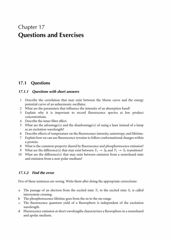
Chapter 17Questions and Exercises
17.1 Questions
17.1.1 Questions with short answers
1 Describe the correlation that may exist between the Morse curve and the energypotential curve of an anharmonic oscillator.
2 What are the parameters that influence the intensity of an absorption band?3 Explain why it is important to record fluorescence spectra at low product
concentrations.4 Describe the inner filter effect.5 What are the advantage(s) and the disadvantage(s) of using a laser instead of a lamp
as an excitation wavelength?6 Describe effects of temperature on the fluorescence intensity, anisotropy, and lifetime.7 Explain how we can use fluorescence tyrosine to follow conformational changes within
a protein.8 What is the common property shared by fluorescence and phosphorescence emission?9 What are the difference(s) that may exist between T1 → S0 and T1 → S1 transitions?
10 What are the difference(s) that may exist between emission from a nonrelaxed stateand emission from a non-polar medium?
17.1.2 Find the error
Five of these sentences are wrong. Write them after doing the appropriate corrections:
a The passage of an electron from the excited state T1 to the excited state S1 is calledintersystem crossing.
b The phosphorescence lifetime goes from the ns to the ms range.c The fluorescence quantum yield of a fluorophore is independent of the excitation
wavelength.d Fluorescence emission at short wavelengths characterizes a fluorophore in a nonrelaxed
and apolar medium.

Questions and Exercises 233
e Fluorophore molecules dissolved in an apolar medium are associated to the solventmolecules by their dipoles.
f The multiple fluorescence lifetimes of a fluorophore are dependent on different factorssuch as the nonrelaxed states of the fluorophore.
17.1.3 Explain
a We have recorded the fluorescence emission spectrum of Trp residues of a protein ata λex of 295 nm using different slits at the excitation and emission wavelengths, andobtained the spectra shown in Figure 17.1. Regardless of the intensity variation, do youobserve any significant difference between the recorded spectra?
b Why does an increase in temperature broaden the spectral bands?c How can we know whether a solution contains one or two fluorophores?d The principle of resonance energy transfer.e The error we can induce if we record the fluorescence spectra of the blank and the
fluorophore solution at two different temperatures.f The principle of studying molecules diffusion in cells with the method of
photobleaching.g Why does an increase in temperature decrease the fluorescence quantum yield?h Why might the information obtained from dynamic fluorescence quenching be different
from that obtained with dynamic phosphorescence quenching?i How can you explain the existence of a fluorescence quantum yield?j What are the difference(s) between isobestic and isoemissive points?
Fluorescenceintensity
(a)
Slits (15/10) 1
Slits (10/10) 2
Slits (5/5) 3
Slits (2.5/2.5) 4
Wavelength
Figure 17.1 Fluorescence emission spectrum of Trp residues within a protein recoded at differentexcitation/emission slits.

234 Principles and Applications of Fluorescence Spectroscopy
17.1.4 Exercises
17.1.4.1 Exercise 1
We have determined the rotational correlation time and the fluorescence intensity of theunique Trp residue of a protein, at the native and the denatured states at three temperatures,5, 17, and 44◦C and obtained the following values:
c (ns) 0.1 5 10 2 1 15I (au) 5 7 10 20 17 15
Assign to each value of c and I the temperature of the measurement and the state ofthe protein. Explain your assignment.
17.1.4.2 Exercise 2
The heme optical density of a hemoprotein and the fluorescence intensity of the unique Trpresidue of the protein are recorded at hydrostatic pressures between 0 and 4 kbar. The tworecorded parameters increase with hydrostatic pressure. Explain in five to seven lines.
17.1.4.3 Exercise 3
We have determined the emission maximum of TNS bound to a protein at two hydrostaticpressures (0 and 5 kbar) and at three different temperatures, −60, 0, and 40◦C (λex =360 nm), and obtained the following results:
0 kbar 5 kbar
−60◦C 420 nm 425 nm0◦C 430 nm 435 nm
40◦C 433 nm 435 nm
Can you explain the results obtained?
17.1.4.4 Exercise 4
We have determined the fluorescence polarization P and the bimolecular diffusion constantkq of oxygen of the unique Trp residue of a protein at three temperatures, 5, 20, and 30◦C,and at two hydrostatic pressures (0–4 kbar), and obtained the following results:
P 0.015 0.03 0.05 0.1 0.2 0.3kq (M−1 s−1) 0.5 × 10⁸ 4 × 10⁸ 8 × 10⁸ 1 × 10⁹ 5 × 10⁹ 9 × 10⁹

Questions and Exercises 235
Assign to each value of P and kq the corresponding temperature and hydrostatic pressure.Explain your assignment in five to seven lines.
17.1.4.5 Exercise 5
The polarization and the rotational correlation time of the unique Trp residue of a proteinhave been measured at two hydrostatic pressures, 0 and 8 kbar, at three temperatures, 5, 17,and 44◦C. The following values are obtained:
P 0.1 0.06 0.05 0.3 0.2 0.44c 2.9 8.5 44.6 1.5 4.4 22.4
Assign to each value of P and c the corresponding temperature and hydrostatic pressure.Explain your assignment in a maximum of seven lines.
17.1.4.6 Exercise 6
The fluorescence lifetime and polarization of an extrinsic probe bound tightly to a sphericalprotein have been measured at different oxygen concentrations. The following data areobtained:
O2 (mM) P τ (ns)
0.218 0.156 150.250 0.178 120.450 0.208 90.700 0.250 6
What is the molecular weight of the protein? The viscosity η at 20◦C is 0.01 g cm−1 s−1.The Boltzman constant k = 1.3805 × 10⁻⁶ g cm2 s−2 K−1. The Avogadro number N =6.022 × 10²³.
17.1.4.7 Exercise 7
The fluorescence intensity and anisotropy of the flavin of a flavoprotein have been measuredfrom 0 to 4 kbar. We notice an increase in the fluorescence intensity and a decrease in thefluorescence anisotropy. Explain the results in five to seven lines.
17.1.4.8 Exercise 8
We have determined the fluorescence intensity and lifetime of the unique Trp residue ofa protein, at the native and denatured states at three temperatures, 5, 17, and 44◦C, and

236 Principles and Applications of Fluorescence Spectroscopy
obtained the following values:
τ 0.1 0.3 0.5 1 3 5 nsI 5 10 20 40 80 100 au
Assign to each value of τ and I the temperature of the measurement and the state of theprotein. Explain your assignment.
17.1.4.9 Exercise 9
Describe a fluorescent method allowing the conformational change of a protein to befollowed with the two probes: Trp residue and TNS.
17.1.4.10 Exercise 10
1 The fluorescence polarization of the unique Trp residue of a monomeric protein hasbeen measured as a function of the temperature over viscosity ratio. The followingvalues have been obtained:
P 0.200 0.190 0.182 0.174T/η 190 260 340 410
Knowing that the value of the limiting polarization at the excitation wavelength is0.24, the rotational correlation time of the protein is 20 ns, and the fluorescence lifetimeof the Trp residue is 2.8 ns, can you tell whether the fluorophore presents residualmotions or not?
2 If we measure the anisotropy decay of the Trp residue of the protein as a functionof time, based on the answer you found in question 1, what would be the expectedresult?
3 The fluorescence intensity of the Trp residue of the protein is measured as a functionof temperature, what will be the result that we should obtain and why? The viscosity η
at 20◦C is 0.01 g cm−1 s−1. The Boltzman constant k = 1.3805 × 10⁻⁶ g cm2 s−2 K−1.The Avogadro number N = 6.022 × 10²³.
17.1.4.11 Exercise 11
Binding experiments have been performed between the fluorophore TNS and aflavodeshydrogenase extracted from the yeast Hansenula anomala. The fluorescencespectrum of the Trp residues of the protein was recorded from 320 to 370 nm, in theabsence and presence of different concentrations of TNS. Two sets of experiments were

Questions and Exercises 237
carried out, one in phosphate buffer pH 7 and one in 6 M guanidine, pH 7. The followingfluorescence intensities (IF) were obtained:
Experiment 1
[TNS] = 0 μM [TNS] = 0.74 μM [TNS] = 0.95 μM
λ (nm) IF λ (nm) IF λ (nm) IF
320 14.2 320 13.3 320 12.5325 16.5 325 15.5 325 14.7330 18.3 330 17.4 330 16.5335 19.3 335 18.5 335 17.6340 19.6 340 18.7 340 17.9342 19.4 342 18.6 342 17.8343.5 19.2 343.5 18.5 343.5 17.7345 19.0 345 18.3 345 17.5350 17.7 350 17.1 350 16.4355 16.1 355 15.5 355 14.9360 14.3 360 13.8 360 13.2365 12.4 365 12 365 11.5370 10.8 370 10.5 370 10.2
[TNS] = 2.33 μM [TNS] = 3.17 μM [TNS] = 3.97 μM
λ (nm) IF λ (nm) IF λ (nm) IF
320 11.8 320 10.8 320 10.5325 13.8 325 12.7 325 12.2330 15.6 330 14.5 330 14335 16.8 335 15.6 335 15.2340 17.3 340 16 340 15.8342 17.2 342 15.9 342 15.8343.5 17.1 343.5 15.9 343.5 15.7345 16.9 345 15.7 345 15.6350 15.9 350 14.75 350 14.75355 14.5 355 13.5 355 13.4360 13.0 360 12.1 360 12.1365 11.3 365 10.5 365 10.4370 10 370 9.4 370 9.3

238 Principles and Applications of Fluorescence Spectroscopy
[TNS] = 4.45 μM [TNS] = 5.18 μM [TNS] = 6.14 μM
λ (nm) IF λ (nm) IF λ (nm) IF
320 10 320 9.7 320 9.2325 11.8 325 11.5 325 10.8330 13.6 330 13.2 330 12.6335 14.9 335 14.4 335 13.8340 15.3 340 14.9 340 14.3342 15.4 342 15.1 342 14.4343.5 15.4 343.5 15.0 343.5 14.4345 15.2 345 14.8 345 14.3350 14.5 350 14.1 350 13.65355 13.3 355 12.9 355 12.5360 12.1 360 11.5 360 11.2365 10.3 365 10.1 365 9.8370 9.2 370 8.9 370 8.7
[TNS] = 6.56 μM [TNS] = 6.98 μM [TNS] = 7.88 μM
λ (nm) IF λ (nm) IF λ (nm) IF
320 8.7 320 8.3 320 8.0325 10.3 325 9.7 325 9.4330 12.0 330 11.4 330 11.0335 13.2 335 12.6 335 12.3340 13.8 340 13.3 340 13.0342 13.8 342 13.35 342 13.0343.5 14.0 343.5 13.45 343.5 13.1345 13.8 345 13.4 345 13.1350 13.2 350 12.7 350 12.5355 12.2 355 11.8 355 11.5360 10.8 360 10.6 360 10.4365 9.5 365 9.3 365 9.2370 8.5 370 8.3 370 8.2

Questions and Exercises 239
[TNS] = 8.68 μM [TNS] = 9.42 μM
λ (nm) IF λ (nm) IF
320 7.6 320 7.1325 9.0 325 8.5330 10.6 330 10.1335 11.3 335 11.3340 12.6 340 12342 12.7 342 12.1343.5 12.8 343.5 12.3345 12.7 345 12.2350 12.2 350 11.8355 11.3 355 11.0360 10.2 360 10.0365 8.9 365 8.9370 8.1 370 8.0
Experiment 2
[TNS] = 0 μM [TNS] = 2 μM [TNS] = 4 μM
λ (nm) IF λ (nm) IF λ (nm) IF
320 7.2 320 7.0 320 6.7325 8.8 325 8.2 325 7.8330 10.7 330 10.0 330 9.7335 12.8 335 12.0 335 11.7340 14.3 340 13.6 340 13.3345 16.2 345 15.6 345 15.2350 17.2 350 16.7 350 16.3355 17.4 355 17.1 355 16.6360 17.0 360 16.9 360 16.4365 16.0 365 16.0 365 15.5370 15.0 370 15.0 370 14.6

240 Principles and Applications of Fluorescence Spectroscopy
[TNS] = 8 μM [TNS] = 12 μM
λ (nm) IF λ (nm) IF
320 6.6 320 6.6325 7.7 325 7.7330 9.5 330 9.5335 11.5 335 11.5340 13.0 340 13.0345 15.0 345 15.0350 16.1 350 16.1355 16.4 355 16.4360 16.1 360 16.1365 15.3 365 15.3370 14.4 370 14.4
1 Plot the spectra of each experiment.2 Can you tell from the data and from the spectra obtained, the buffer in which each
experiment was carried on? Explain your answer.3 Can you give a logical explanation of the slight shift observed in the first experiment?4 Why is this shift not observed in the second experiment?5 The data shown before are from spectra not corrected for the inner filter effect. The
optical density measured at the excitation wavelength (280 nm) and at two emissionwavelengths, 335 for experiment 1 and 355 for experiment 2, gives the following values:
Experiment 1
OD[TNS] Volume in the(μM) cuvette (μl) λex = 280 nm λem = 335 nm
0 1060 0.086 0.0080.74 1061.5 0.092 0.0160.95 1063 0.107 0.0262.33 1064.5 0.116 0.0303.17 1066 0.130 0.0403.97 1067.5 0.143 0.0474.45 1069 0.151 0.0525.18 1070.5 0.162 0.0596.14 1072 0.181 0.0676.56 1073.5 0.190 0.0726.98 1075 0.200 0.0787.88 1076.5 0.210 0.0848.68 1078 0.223 0.0929.42 1079.5 0.234 0.099

Questions and Exercises 241
Experiment 2
OD[TNS] Volume in the(μM) cuvette (μl) λex = 280 nm λem = 335 nm
0 1100 0.090 0.0122 1110 0.120 0.0344 1120 0.147 0.0456 1130 0.185 0.0588 1140 0.214 0.070
Correct the fluorescence intensities at 335 and 355 nm for the optical densities. What canyou conclude?
The optical densities measured with a spectrophotometer were obtained with an opticalpath length equal to 1 cm. However, optical path lengths equal to 1 and 0.4 cm were usedfor the emission and excitation wavelengths, respectively.
17.1.4.12 Exercise 12
O-Nitrophenyl glactoside hydrolysis with β-galactosidase in the absence and presence ofthree inhibitors, O-nitrophenyl β-D-thiogalactoside (ONPTG), maltose, and melibiose, wasstudied at 25◦C in pH 7.5 buffer. Table 17.1 shows the optical densities at 410 nm of thePNP formed, expressed per minute.
Table 17.1 Optical densities at 410 nm of PNP obtained by minute.
[Substrate] v1 v2 v3(M) vo (3 × 10⁻⁴ M of ONPTG) (0.26 M of maltose) (0.17 M of melibiose)
2.5 × 10⁻⁵ 0.033 0.018 0.0165 0.0275 × 10⁻⁵ 0.055 0.033 0.0275 0.0411 × 10⁻⁴ 0.0825 0.055 0.041 0.0552.5 × 10−4 0.118 0.091 0.059 0.0695 × 10⁻⁴ 0.138 0.118 0.069 0.0751 × 10⁻³ 0.15 0.138 0.075 0.079
Plot v = f ([S]) and determine the types of inhibition. Calculate the kinetic parameters.
17.2 Solutions
17.2.1 Questions with short answers
1 Describe the correlation that may exist between the Morse curve and the energy potentialcurve of a anharmonic oscillator.

242 Principles and Applications of Fluorescence Spectroscopy
R1. Within a molecule, the stretching of the molecular bond lets the atoms comecloser and move away one from each other. The Morse curve describes the potentialenergy induced by this stretching. At short distances, the repulsive forces are dominant,while at long distances, the attractive forces are dominant. However, when thedistance that separates the two atoms within the bond is too important, the attractiveforces are no longer efficient, and the Morse curve will look like an anharmonicoscillator.
2 What are the parameters that influence the intensity of an absorption band?R2. The position of the nuclei at the moment of the electronic transition and thepopulation of molecules that have reached the excited state.
3 Explain why it is important to record fluorescence spectra at low product concentrations.R3. A high concentration may increase the optical density at the excitation and/orthe emission wavelengths. This will distort the fluorescence emission spectrum bydecreasing the real fluorescence intensity and by shifting the emission peak.
4 Describe the inner filter effect.R4. At a high optical density at the excitation and/or emission wavelengths, a distortionof the fluorescence emission spectrum is observed. A fluorescence intensity decrease isobserved, and the emission peak is shifted.
5 What are the advantage(s) and the disadvantage(s) of using a laser instead of a lamp asan excitation source?R5. The energy of a laser is higher than that of a lamp, thus allowing one to work at lowfluorophore concentrations. However, since fluorophores are light-sensitive, excitationwith a laser could accelerate the photo-bleaching rate.
6 Describe the temperature effects on fluorescence intensity, anisotropy, and lifetime.R6. Temperature favors the deactivation processes other than fluorescence andso decreases the fluorescence intensity, quantum yield, and lifetime. Temperatureincreases the local motions of the fluorophores and so decreases the value of thepolarization.
7 Explain how can we use tyrosine fluorescence to follow conformational changes within aprotein.R7. Fluorescence of tyrosine in protein is generally quenched as a result of the tertiarystructure of the protein. A structural modification of the protein would affect thefluorescence properties of the protein, including those of the tyrosine. Thus, in somecases, one can observe an increase in the fluorescence intensity at 303 nm and thequantum yield of the tyrosine and a decrease in its anisotropy.
8 What is the common property shared by fluorescence and phosphorescence emission?R8. Photon emission.
9 What are the difference(s) that may exist between T1 → So and T1 → S1 transitions?R9. T1s → So transition is possible since T1 is energetically higher than So.T1 → S1 transition is not possible because T1 is energetically lower than S1.
10 What are the difference(s) that may exist between emission from a nonrelaxed state andemission from a non-polar medium?R10. Emission from a nonrelaxed state means that it occurs before the dipolereorientation of the solvent molecules or the dipole of the amino acids of thefluorophore binding site. Emission from a non-polar medium means that thefluorescence occurred after the inducing by the fluorophore of a dipole in the medium.

Questions and Exercises 243
17.2.2 Find the error
Five of these sentences are wrong. Write them out after doing the appropriate corrections:
1 The passage of an electron from the excited state T1 to the excited state S1 is called intersystemcrossing.R1. The passage of an electron from the excited state S1 to the excited state T1 is calledintersystem crossing.
2 The phosphorescence lifetime goes from the ns to the ms range.R2. The phosphorescence lifetime stands from the ms to the s, min, or h range.
3 The fluorescence quantum yield of a fluorophore is independent of the excitation wavelength.R3. The sentence is correct.
4 Fluorescence emission at short wavelengths characterizes a fluorophore in a nonrelaxed andapolar medium.R4. Fluorescence emission at short wavelengths characterizes a fluorophore in anonrelaxed or non-polar medium.
5 Fluorophore molecules dissolved in a non-polar medium are associated to the solventmolecules by their dipoles.R5. Fluorophore molecules dissolved in a polar medium are associated to the solventmolecules by their dipoles.orThe dipoles of fluorophore molecules dissolved in a polar medium are associated withthe dipoles of the solvent molecules.orThe dipoles of fluorophore molecules dissolved in a non-polar medium are associatedwith the induced dipoles of the solvent molecules.
6 The multiple fluorescence lifetimes of a fluorophore are dependent on different factors suchas the nonrelaxed states of the fluorophore.R6. The multiple fluorescence lifetimes of a fluorophore are dependent on differentfactors such as the nonrelaxed states of the fluorophore emission.
17.2.3 Explain
a At large slits, vibrational transitions are not observed on the emission spectra.b Why does a temperature increase broaden the spectral bands?
Rb. Temperature increases the frequency of molecular collisions. The vibrationaltransitions of the nuclei are badly resolved. This will induce a broadening of the spectralbands.
c How can we know whether a solution contains one or two fluorophores?Rc. The fluorescence emission of a solution containing two fluorophores varies withexcitation wavelength, which is not the case in the presence of one fluorophore.
d The principle of resonance energy transfer.Rd. The electron of the excited molecules induces an oscillating electric field that excitesthe electrons of the acceptor molecules.
244 Principles and Applications of Fluorescence Spectroscopy
e The error we can induce if we record the fluorescence spectra of the blank and the fluorophoresolution at two different temperatures.Re. In principle, the blank is not fluorescing. However, one should subtract the Ramanspectrum of the blank from the recorded fluorescence spectrum of the fluorophore.Therefore, the temperature should be the same for both spectra; otherwise, an errorcould be induced in determining the real intensity of the fluorophore emission.
f The principle of studying molecules diffusion in cells with the method of photobleaching.Rf. We induce an irreversible photo-bleaching of fluorophore molecules within a specificregion of the cell. The appearance of fluorescence in this area after a short time is theresult of fluorophore diffusion from other cell areas to the irradiated area.
g Why does an increase in temperature decrease the fluorescence quantum yield?Rg. Increasing the temperature will induce an increase in the Brownian motions andthe intramolecular fluctuations. Therefore, deactivation of the excited singlet state S1
via nonradiative processes will be favored, and there will be fewer emitted photons. Thisinduces a decrease in the quantum yield.
h Why might the information obtained from dynamic fluorescence quenching be differentfrom that obtained with dynamic phosphorescence quenching?Rh. Since the phosphorescence lifetime is longer than the fluorescence lifetime, theinformation obtained is within two different timescales and so can be different.
i How can you explain the existence of a fluorescence quantum yield?Ri. Since different processes deactivate the excited state of the molecule, there arefewer photons emitted via fluorescence than photons originally absorbed by thefluorophore.
j What are the difference(s) that exist between isobestic and isoemissive points?Rj. We use the term isobestic when we are dealing with absorption spectroscopy and theterm isoemissive when we are dealing with fluorescence spectroscopy.
17.2.4 Exercises solutions
17.2.4.1 Exercise 1
At a specific temperature, in the native state, the protein is more compact than in thedenatured state. Thus, the motion of the fluorophore in the native state is slower than itsmotion in the denatured state. Therefore, the rotational correlation time of the fluorophoreis longer in the native state.
For a specific protein state, increasing the temperature will accelerate the motion of thefluorophore. Therefore, the rotational correlation time will be shorter when the temperatureis higher.
In the native state, the compactness of the protein increases the interaction between thefluorophore and the surrounding amino acids, thereby decreasing the fluorescence intensity.Thus, the fluorescence intensity should be lower in the native state than when the protein isdenatured.
Increasing the temperature will facilitate deactivation of the fluorophore via thenonradiative process and so will decrease the temperature.

Questions and Exercises 245
Native state Denatured state
5◦C 10 au 2 ns 20 au 15 ns17◦C 7 au 1 ns 17 au 10 ns44◦C 5 au 0.1 ns 15 au 5 ns
17.2.4.2 Exercise 2
At 0 kbar, the protein is not denatured but disrupted. Hydrostatic pressure favors hemedisplacement from its binding site, the heme pocket. Hemin (free heme) will absorb morethan bound heme. In the absence of heme in the protein, energy transfer from Trp residuesto heme decreases, thereby inducing an increase in the fluorescence intensity.
17.2.4.3 Exercise 3
TNS fluorescence will characterize the state of the protein. At 5 kbar, the protein is not yetdenatured, although its tertiary structure is stabilized.
At low temperatures, TNS emission will occur from a nonrelaxed state, and the emissionpeak will be blue-shifted compared to the spectrum obtained at high temperatures. This iswhy there is a shift of 10 nm between the spectra recorded at −60 and 0◦C.
In the native state, the shift observed between 0 and 40◦C is 3 nm, indicating that thestructure around TNS is not loose. Hydrostatic pressure destabilizes the tertiary structureof the protein. In this case, between 0 and 40◦C, there is no shift in the emission peak.
17.2.4.4 Exercise 4
At 0 kbar, the protein is more compact than at 4 kbar. Thus, motions and fluctuations withinthe protein are weaker at 0 kbar. Therefore, for the same temperature, P is higher at 0 kbarthan at 4 kbar, and kq is weaker.
When the temperature increases, protein motions increase, accompanied by a decreasein the value of P . Also, oxygen diffusion increases, accompanied by an increase in kq value.
0 kbar 4 kbar
P kq P kq
5◦C 0.3 0.5 × 10⁸ 0.05 1 × 10⁹
20◦C 0.2 4 × 10⁸ 0.03 5 × 10⁹
30◦C 0.1 8 × 10⁸ 0.01 9 × 10⁹
17.2.4.5 Exercise 5
At low temperatures, motions are weak, and the rotational time is high. Also, weak motionsinduce a high polarization value P .
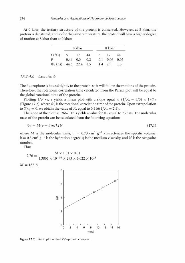
246 Principles and Applications of Fluorescence Spectroscopy
At 0 kbar, the tertiary structure of the protein is conserved. However, at 8 kbar, theprotein is denatured, and so for the same temperature, the protein will have a higher degreeof motion at 8 kbar than at 0 kbar:
0 kbar 8 kbar
t (◦C) 5 17 44 5 17 44P 0.44 0.3 0.2 0.1 0.06 0.05c (ns) 44.6 22.4 8.5 4.4 2.9 1.5
17.2.4.6 Exercise 6
The fluorophore is bound tightly to the protein, so it will follow the motions of the protein.Therefore, the rotational correlation time calculated from the Perrin plot will be equal tothe global rotational time of the protein.
Plotting 1/P vs. τ.. yields a linear plot with a slope equal to (1/Po − 1/3) × 1/P
(Figure 17.2), where P is the rotational correlation time of the protein. Upon extrapolationto T/η = 0, we obtain the value of Po equal to 0.416(1/Po = 2.4).
The slope of the plot is 0.2667. This yields a value for P equal to 7.76 ns. The molecularmass of the protein can be calculated from the following equation:
P = M (ν + h)η/kTN (17.1)
where M is the molecular mass, ν = 0.73 cm3 g−1 characterizes the specific volume,h = 0.3 cm3 g−1 is the hydration degree, η is the medium viscosity, and N is the Avogadronumber.
Thus
7.76 = M × 1.01 × 0.01
1.3805 × 10−16 × 293 × 6.022 × 1023
M = 18715.
0 2 4 6 8 10 12 14 160
2
4
6
8
1/P
� (ns)
Figure 17.2 Perrin plot of the DNS–protein complex.
Questions and Exercises 247
17.2.4.7 Exercise 7
Up to 4 kbar, protein is not denatured. However, slight structural changes can be observed,inducing flavin release from its binding site. Free flavin in solution has almost no interactionswith the protein, and so energy transfer between the flavin and the amino acids of its bindingsite decreases, which induces an increase in the fluorescence intensity of the co-factor.
The motions of free flavin in solution are much more important than those of boundflavin. Thus, the anisotropy of flavin will decrease with increasing hydrostatic pressure.
17.2.4.8 Exercise 8
The tertiary structure of the protein induces a high energy transfer between the Trp residueand the neighboring amino acids. This induces low values in the fluorescence parametersof the Trp residue in the native state in comparison to those measured when the protein isdenatured, and so the energy transfer is weak.
A temperature increase induces energy loss via the nonradiative process, therebydecreasing the values of the fluorescence parameters.
Native state Denatured state
IF τ IF τ
5◦C 20 0.5 100 517◦C 10 0.3 80 344◦C 5 0.1 40 1
17.2.4.9 Exercise 9
A Trp residue embedded in the protein matrix will in principle fluoresce with a maximumlocated at 330 nm. A conformational change may induce a displacement of the Trp residuetoward the protein surface. Thus, a shift of the maximum peak to the highest wavelengths(340–350 nm) will be observed.
A structural modification of the protein could induce the displacement of the TNS fromits binding site and so the fluorescence intensity decrease in the fluorophore.
17.2.4.10 Exercise 10
Let us plot the Perrin plot 1/P vs. T/η and calculate the rotational correlation time c
and the polarization P(0) at T/η = 0. If c is equal to that of the protein and P(0) to thelimiting polarization, then the fluorophore is bound tightly to the protein. Otherwise, thefluorophore displays free and independent motions.

248 Principles and Applications of Fluorescence Spectroscopy
17.2.4.11 Exercise 11
1.
320 330 340 350 360 3706
8
10
12
14
16
18
20
14
1F
luor
esce
nce
inte
nsity
(au
)
Wavelength (nm)
Figure 17.3 Fluorescence spectra of Trp residues of Hansenula anomala flavodehydrogenase, in theabsence (spectrum 1) and presence (spectra 2–14) with increasing concentrations of TNS. The spectraobtained are from Experiment 1.
320 330 340 350 360 370
6
8
10
12
14
16
18
4;5
1
Flu
ores
cenc
e in
tens
ity (
au)
Wavelength (nm)
Figure 17.4 Fluorescence spectra of Trp residues of Hansenula anomala flavodehydrogenase, in theabsence (spectrum 1) and presence (spectra 2–5) of increasing concentrations of TNS.The spectra obtainedare from Experiment 2.

Questions and Exercises 249
2 Experiment 1 was carried out in phosphate buffer, pH 7. In fact, the fluorescencemaximum is located at 340 nm, indicating a fluorescence arising from a structuredprotein. Experiment 2 was carried out in Guanidine, since the Trp residues emit from adenatured state (355 nm). Guanidine denatures proteins.
3 The slight shift to the red observed in the presence of TNS could be simply the resultof the inner filter effect due to the absorption of TNS, or it may indicate a slightconformational change of the protein around the Trp residues. In order to find outwhich of the two cases we have here, we have to replot the spectra after correcting theintensities for the inner-filter effect. If the peaks of the corrected spectra shift to 340 nm,the red-shift observed is the result of the inner filter effect. However, if the positions ofthe peak do not change, the red shift observed is the result of a slight conformationalchange around the Trp residues.
4 In the presence of 6 M guanidine, the protein is completely denatured. Trp residues arefully exposed to the solvent. In this case, the interaction between the protein and TNS isweak, almost non-existent. Therefore, the addition of TNS to the protein will not affectthe fluorescence spectrum of the Trp residues of the protein.
5 First, we should remember that the fluorescence intensities shown are corrected fromthe background intensities of the buffer solution or from guanidine solution. Therefore,observed fluorescence intensities should be corrected for the dilution, and finallycorrections are made for the absorption at the excitation and emission wavelengthsusing the following equation:
Fcorr = Fvol × 10[OD(em)+OD(ex)]/2
where Fcorr is the corrected fluorescence intensity for the inner filter effect, andOD(em) and OD(ex) are the optical densities at the excitation and emission wavelengths,respectively.
Fluorescence measurement of the Trp residues of the protein in the absence of TNS wasperformed in a total volume equal to 1060 and 1100 for the native and denatured proteins,respectively. Addition of TNS increases the initial volume and so dilutes the protein solution.Therefore, in order to see the real effect of TNS addition on the protein fluorescence, weshould correct the fluorescence intensities for the dilution effect. In the present experiments,we can see that the volume of TNS added to the protein solution is small, and so correctionsshould have only a minor effect. However, let us do these corrections using the followingequation:
Fvol = Frec × volume in the presence of TNS
volume in the absence of TNS

250 Principles and Applications of Fluorescence Spectroscopy
Experiment 1
Correction for the volume
[TNS] (μM) Volume in the cuvette (μl) Irec Ivol
0 1060 19.3 19.30.74 1061.5 18.5 18.530.95 1063 17.6 17.652.33 1064.5 16.8 16.873.17 1066 15.6 15.6883.97 1067.5 15.2 15.304.45 1069 14.9 15.035.18 1070.5 14.4 14.546.14 1072 13.8 13.966.56 1073.5 13.2 13.376.98 1075 12.6 12.787.88 1076.5 12.3 12.498.68 1078 11.3 11.499.42 1079.5 11.3 11.51
Correction for the inner filter effect
The optical densities are obtained with a spectrophotometer using a path length equal to1 cm. However, when fluorescence experiments were performed, the optical path lengthupon excitation was equal to 0.4 cm. Thus, the real optical density at the excitationwavelength is equal to that measured on the spectrophotometer divided by 2.5.
λex = 280 nm λem = 335 nm[TNS] (μM) OD(experiment) OD(experiment) fc Ivol Icorr
0 0.0344 0.008 1.05 19.3 20.270.74 0.0368 0.016 1.063 18.53 19.700.95 0.0428 0.026 1.083 17.65 19.122.33 0.0464 0.030 1.092 16.87 18.433.17 0.052 0.040 1.11 15.688 17.423.97 0.0572 0.047 1.127 15.30 17.244.45 0.0604 0.052 1.138 15.03 17.105.18 0.0648 0.059 1.153 14.54 16.776.14 0.0724 0.067 1.174 13.96 16.396.56 0.076 0.072 1.186 13.37 15.866.98 0.080 0.078 1.200 12.78 15.347.88 0.084 0.084 1.213 12.49 15.158.68 0.0892 0.092 1.232 11.49 14.169.42 0.0936 0.099 1.248 11.51 14.37
Questions and Exercises 251
One can notice that after correction for the inner filter effect, one can still observe adecrease in the fluorescence intensities of the Trp residues. This decrease is a result of theTNS binding to the flavodehydrogenase.
Experiment 2
Correction for the volume
[TNS] (μM) Volume in the cuvette (μl) Irec Ivol
0 1100 17.4 17.402 1110 17.1 17.264 1120 16.6 16.906 1130 16.4 16.858 1140 16.4 17.0
Correction for the inner filter effect
λex = 280 nm λem = 355 nm[TNS] (μM) OD(experiment) OD(experiment) fc Ivol Icorr
0 0.0360 0.012 1.057 17.40 18.402 0.0480 0.034 1.099 17.26 18.964 0.0588 0.045 1.127 16.90 19.006 0.0740 0.058 1.164 16.85 19.618 0.0856 0.070 1.196 17.00 20.33
One can see that after correction for the dilution and the inner filter effect, the measuredintensities in the presence of TNS reach that measured for the protein alone. This indicatesthat binding of TNS to the flavodehydrogenase does not occur, and the protein has lost itsspecific binding site for the TNS.
This experiment can be repeated with other proteins such as bovine serum albumin, aprotein that is commercially very easily available.
17.2.4.12 Exercise 12
Plotting the velocity expressed as optical density per minute vs. substrate concentrations inthe absence and presence of the three inhibitors yields the results shown in Figure 17.5.
The curves shown indicate that ONPTG, maltose, and melibiose, in the range of theconcentrations used, inhibit the O-nitrophenyl galactoside hydrolysis rate. We can see fromthe curves that a plateau is not reached at the high concentrations of inhibitors, meaningthat the maximum velocity VM is not reached. Thus, in order to determine VM and KM,reciprocal plots should be drawn (Figure 17.6).
ONPTG acts as a competitive inhibitor, maltose as a noncompetitive inhibitor, andmelibiose as a noncompetitive inhibitor.
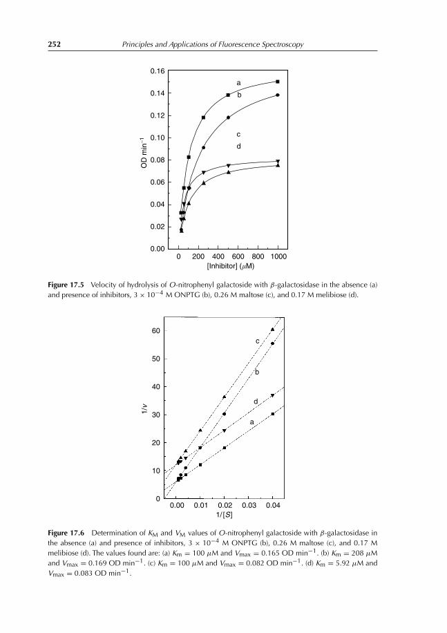
252 Principles and Applications of Fluorescence Spectroscopy
0 200 400 600 800 10000.00
0.02
0.04
0.06
0.08
0.10
0.12
0.14
0.16
OD
min
−1
[Inhibitor] (�M)
a
b
c
d
Figure 17.5 Velocity of hydrolysis of O-nitrophenyl galactoside with β-galactosidase in the absence (a)and presence of inhibitors, 3 × 10⁻⁴ M ONPTG (b), 0.26 M maltose (c), and 0.17 M melibiose (d).
0.00 0.01 0.02 0.03 0.040
10
20
30
40
50
60
1/v
1/ [S]
a
b
c
d
Figure 17.6 Determination of KM and VM values of O-nitrophenyl galactoside with β-galactosidase inthe absence (a) and presence of inhibitors, 3 × 10⁻⁴ M ONPTG (b), 0.26 M maltose (c), and 0.17 Mmelibiose (d). The values found are: (a) Km = 100 μM and Vmax = 0.165 OD min−1. (b) Km = 208 μMand Vmax = 0.169 OD min−1. (c) Km = 100 μM and Vmax = 0.082 OD min−1. (d) Km = 5.92 μM andVmax = 0.083 OD min−1.

Index
1-Anilino-8-naphthalene sulfonate (ANS), 109,115, 118, 119, 121
Absorption, 1, 34, 42, 48, 61, 63, 69, 76, 88, 91,108, 191, 198, 232
Absorption spectrum, 2–4, 6, 7, 16–18, 21, 22,35, 36, 79, 82, 84, 91, 94, 104, 115, 116,119, 124, 150, 169, 170, 172, 197, 200
Acridine Orange, 197Acrylamide, 144Alpha-amylase, 59, 61, 67, 69, 70, 73, 77α-l-fucose, 190α1-Acid glycoprotein, 13, 15–18, 134, 150Anisotropy, 160–162, 166, 235, 236Arrhenius activation energy, 155Association constant, Ka, 148, 153, 174–6, 194,
211, 215, 218
Beer-Lambert-Bouguer law, 4, 5, 13, 37, 38, 126Benzo(a) pyrene, 222β-galactosidase, 34, 35, 38–40, 42, 43, 47, 48, 56,
57, 241β-lactoglobulin, 135Bimolecular diffusion constant, kq, 141, 144,
150, 219, 234Bioluminescence resonance energy transfer,
BRET, 204, 205, 207Bovine serum albumin, BSA, 42, 118, 120,
210–212, 215, 218Bradford method, 42
Calcofluor White, 13, 16, 18, 131Catalytic constant, kcat, 25, 30Cesium ion, 144Chromophore, 2, 6, 89, 91Coomassie blue, 42Cytochrome b2 core, 126Cytochrome P-450, 203
Dipole relaxation, 112, 113Dissolved organic matter, DOM, 152DNA, 168–70, 172, 173, 175, 177, 180, 197, 220,
222, 224, 227, 231Dynamic quenching, 140, 143, 157, 184
Electron spin, 90, 91Emission spectrum, 91, 93–5, 101, 115, 117, 124,
132, 171, 173, 197, 211, 242Energy transfer, 106, 140, 202Energy transfer efficiency, 211, 218Enzymatic activity, 21, 40Equilibrium constant, Keq, 48, 50, 52, 54Ethidium bromide, 110, 115, 168, 169, 171, 172,
175, 177, 179, 180Europium cryptate, 200, 201Excitation, 1, 91, 160Excitation spectrum, 93, 95, 115, 117, 120, 123,
136, 173, 179, 198
First-order kinetics, 28Flavin adenine dinucleotide, FAD, 108Flavin mononucleotide, FMN, 108, 155, 157,
247Fluorescein, 108, 127, 184, 187, 193, 194Fluorescence, 88, 91, 232Fluorescence intensity, 139, 155, 211Fluorescence lifetime, 96, 97, 139, 149, 155, 166,
243Fluorescence microscopy, 225, 226Fluorescence quantum yield, 94, 101, 111, 139,
141, 232, 233, 243, 244Fluorophore, 89, 92, 102, 112, 146, 179, 243, 246Förster energy transfer, 197, 198, 200, 202, 204,
219, 233, 243Franck-Condon Principle, 1Frequency-domain method, 98
254 Index
Front-face spectroscopy, 135Fulvic acid, 152
Green fluorescent protein, GFP, 204, 205Guanidine chloride, 47, 48, 54–6, 124, 237, 249
Heat treatment, 69Heme, 6, 164, 204, 234, 245Heparanase, 201Homogeneous time-resolved fluorescence, 200,
201Humic substances, 152, 153Hydrolysis, 41, 59Hydrostatic pressure, 234, 235, 245
Inhibition constant, KI, 46Inner filter effect, 95, 121, 125, 129, 185, 232,
240, 242, 249, 250Intrinsic polarization, 163, 166Iodide ion, 144, 184Isobestic point, 84, 171, 233, 244Isoemissive point, 233, 244
Jablonski diagram, 88, 89, 154
Lactate dehydrogenase, LDH, 21Lactotransferrin, LTF, 190–192, 194Lectin, 146, 149, 157, 184, 187, 191, 192, 194
4-Methyl-2-nitrophenol, mNPH, 82, 84, 854-Methyl-2-nitrophenolate, mNP, 82Maltose, 63Melting temperature, 135, 136, 180Membrane, 199Michaëlis constant, KM, 25, 30–32, 44, 47, 251Molar extinction coefficient, 4, 6, 13, 16, 18, 19,
22, 35–8, 48, 80, 94, 105, 128, 131, 169,175, 210
Morse curve, 1, 232, 242Multifrequency, 100Multiplicity, 90Myoglobin, 164
NADH, 21, 23, 108, 115, 118, 123
Olive tail moment, 231Optical Density (O.D), 5, 18, 36–42, 44–8, 55,
47, 80, 81, 83–6, 94, 95, 101, 120, 128,129, 135, 169–71, 175, 176, 179, 211,234, 240–242, 250, 251
Oxygen, 144, 234, 245Oxygen diffusion, 143
Paranitrophenol, PNP, 34–9, 41, 42, 46, 48Particulate organic carbon, POC, 152Perrin plot, 163, 164, 166, 189, 246pH, 36, 39, 51, 64, 80, 81, 83, 84, 212Phenylalanine, 3, 6, 17, 104Phosphorescence, 232, 243Photobleaching, 233, 244pK, 79–81, 83–6Polarization, 160–162, 177, 187, 235, 245Polarization spectrum, 162Polycyclic aromatic hydrocarbons, PAH, 222Porphyrin, 4, 141, 143, 162, 164Progesterone, 15Protein structure, 104Protonation constant, 79Pyruvate, 21
Quencher, 148, 150
Raman, 102Rayleigh, 102Rhodamine, 108, 199Riboflavin, 115Rotational correlation time, 164, 166, 189, 234,
235, 246
Selective quenching, 145, 146Serotransferrin, STF, 190–192, 194Soret band, 6Spectrofluorometer, 93Standard Gibbs free energy, �G◦′, 51, 52, 54Starch, 59, 61, 64, 66, 67, 70Static quenching, 149Stern-Volmer constant, KSV, 141, 144, 146,
185, 219Stokes shift, 93, 94, 118, 122Strobe method, 98Sucrose, 188
2,p-Toluidinylnaphthalene-6-sulfonate (TNS),15, 109, 115, 118, 123, 149, 157, 210–212,215, 219, 234, 236, 245, 249, 251
Temperature, 40, 66, 135, 155, 157, 180, 232,234, 244, 245
Tetranitromethane, TNM, 105Thermal motions, 3Thermal quenching, 157Time-correlated single-photon counting
(TCSPC) method, 97

Index 255
Time-resolved anisotropy, 166Total organic carbon, TOC, 152Triglyceride, 136Tryptophan, 3, 16, 17, 104, 115, 125, 132, 146,
149, 203, 211, 219, 233, 234, 236, 247
Tyrosine, 3, 6, 17, 104, 105, 132, 134, 232, 242
Vanadate-containing enzyme vanadiumchloroperoxidase, 6, 9, 11
Vitamin A, 135


Color plate 6.2 Methylnitrophenol dissolved in 10 mM Tris buffer at pHs ranging from 2 (far left) to 12(far right). The colorless protonated methylnitrophenol turns yellow when the pH increases.
Color plate 12.4 Fluorescence cuvettes containing ethidium bromide (left) and ethidium bromide–DNAcomplex (right) solutions.
0
34
12
Color
plate16
.7Im
ages
ofco
mets(from
lymph
ocytes),staine
dwith
DAPI.The
serepresen
tclasses
0–4,
asused
forvisual
scoring.
Source:C
ollin
s,A.R.(20
04).
MolecularBiotechnology,2
6,24
9–26
1.Rep
rinted
with
perm
ission
from
Hum
anaPressInc.
01
34
2
Color
plate16
.8CHO
cells
treatedwith
ethy
lmetha
nesulfo
nate;Magnific
ation35
0×.Cou
rtesyof
Dr.AlokDha
wan
,Indu
strial
Toxico
logy
ResearchCen
tre,
Mah
atmaGan
dhiM
arg,
Luckno
w,U
P.www.com
etassayind
ia.org
andwww.com
etassayind
ia.org/protoco
ls.htm
.

Color
plate
16.9
Com
ettest
for
lymph
ocyte
cells
inthree
states:no
rmal,ap
optotic
,an
dne
crotic.Th
eread
ercan
refer
tothe
follo
wing
site:
www.com
etassayind
ia.org
andwww.com
etassayind
ia.org/protoco
ls.htm
.