principle of link evaluation - semantic scholar

Communications and Network, 2009, 06-19 doi:10.4236/cn.2009.11002 Published Online August 2009 (http://www.scirp.org/journal/cn)

Copyright © 2009 SciRes CN

Principle of Link Evaluation

Jinbao ZHANG1, Hongming ZHENG2, Zhenhui TAN3, Yueyun CHEN4 1,3Institution of Electronics and Information, Beijing JiaoTong University, Beijing, China

2Intel China Research Centre, Beijing, China 4University of Science and Technology Beijing, Beijing, China

Email: [email protected], [email protected], 3zhhtan@ bjtu.edu.cn, [email protected]

Abstract: Link Evaluation (LE) is proposed in system evaluation to reduce complexity. It is important to practical systems also for link adaptation. Current algorithms for link evaluation are developed by simulation method, lacking of theoretical description. Although they provide some good accuracy for some scenarios, all of them are not universal. With the help of information theory, a universal principle of link evaluation is pro-posed in this paper, which explains current algorithms and leads to a universal algorithm to implement link evaluation for common wireless transmissions.

This paper proposes an Extended Received Block Information Rate (ERBIR) algorithm for universal link evaluation, which is extended from current RBIR algorithm by the help of the principle presented in this paper. Mainly the universality and accuracy are highlighted. Simulation results verify all the algorithms mentioned in this paper. Both the principle and ERBIR are validated by simulation with various wireless scenarios.

Keywords: link evaluation, information theory, MIMO, OFDM, WiMAX II 1. Introduction

LINK evaluation aims to estimate the instant perform-ance of transmissions for given channel status informa-tion (CSI), by a computational model with reasonable complexity.

As to wireless transmissions, due to macro and micro fading, the CSI is varying within both time and fre-quency domains, so fading will influence wireless trans-mission a lot. Consequently, link evaluation is significant to analysis and design for real wireless system.

For that the instant performance for wireless trans-missions under given CSI can be computed by link evaluation quite simply and accurately, it is possible for System Level Simulation (SLS) to hold down real cod-ing and decoding procedures, reducing a lot of com-plexity [1]. Meanwhile, wireless system can dynami-cally choose the proper transmitting mode with the help of link evaluation to enhance system performance, which is referred as link adaptation [1-3].

Accuracy is very important to link evaluation. For SLS, obviously it directly determines if the simulation results are reasonable. For link adaptation, accurate link evalua-tion ensures that the transmitting mode is selected prop-erly. If the link performance is overestimated, the trans-mitter will always choose a mode which can not be sup-ported by instantaneous CSI, introducing too much transmission error; while the link performance is under-estimated, potential gain exists. Both of the above cases will lead to loss of system performance.

Currently, there are several algorithms to implement

link evaluation, like Effective Exponential Signal-to- noise-ratio Mapping (EESM) [4], Mean Instantaneous Capacity (MIC) [5], Received Block Information Rate (RBIR) [6] and Mean Mutual Information per Bit (MMIB) [7]. Here RBIR and MMIB are Mean mutual Information (MI) based algorithms, with different RBIR calculation. Unfortunately, all of them are just simulation methods, lacking of theoretical analysis. Moreover, when it comes to nonlinear detection, there are still problems with all these algorithms mentioned above.

This paper proposes a universal principle for link evaluation, and extends RBIR to common wireless sce-narios. Firstly, background knowledge is introduced, including models of common transmission and link evaluation; a universal principle for link evaluation is proposed; and then RBIR is extended to ERBIR with the help of this principle. Simulation results show that the proposed algorithm provides more accuracy for different scenarios. Finally, conclusions are drawn.

2. Background

To analyze link evaluation, common models of wireless transmission and link evaluation are presented in this section.

2.1 Common Model of Wireless Transmission

Following assumptions are made for analysis in this pa-per.

1) Multi-Input Multi-Output Orthogonal Frequency Division Multiplexing (MIMO OFDM) is adopted in wireless transmission. NT and NR indicate the number of

PRINCIPLE OF LINK EVALUATION 7

transmitting and receiving antennas respectively. NOFDM indicates the number of subcarriers in OFDM symbol. As to SISO or single subcarrier case, there is NT= NR=1 or NOFDM=1;

2) Perfect channel estimation and the channel response is flat fading on each OFDM subcarrier;

3) Detection with interference cancellation is not taken into consideration;

4) Source bits are random and iterative coding and decoding is used, for example Turbo;

5) Link evaluation interests in statistical BLock Error Rate (BLER) [1] for given CSI. Let Nu indicate the number of subcarriers mapped to the interested wireless resource block.

6) Modulation and Coding Scheme (MCS) levels are set to QPSK 1/2, QPSK 3/4, 16QAM 1/2, 16QAM 3/4, 64QAM 1/2, 64QAM 2/3, 64QAM 3/4 and 64QAM 5/6, referred to MCS 1~8 respectively.

Disregarding subcarrier index, MIMO OFDM trans-mission can be written as [2]

y = HcFx + HIxI + n (1)

where y is NR×1 dimensional receiving signal vector; Hc is NR×NT channel response matrix; F is NT×NS transmit-ting precoding matrix; x is NS×1 independent transmit-ting signal vector, with unit transmitting power; HI is NR×NS interference channel response matrix; xI is NS×1 independent interference signal vector, with unit trans-mitting power; n is NR×1 AWGN vector, which is con-sisted of NR independent AWGN elements with power of σ2 (given SNR, σ2=10−SNR/10). So this MIMO OFDM transmission is effective to

y = Hex + ne; ||He||F2 = 1; ExxH = I(NS);

He = T−1HcF / || T−1HcF ||F; TTH = HI HIH +σ2I(NR);

EneneH =σe

2I(NR); σe2= 1 / || T−1HcF ||F

2 (2)

See Appendix A for a proof. Here He is NR×NS effec-tive channel response matrix. ||A||F refers to the Frobenius norm of matrix A. I(N) is N×N identity matrix. σe

2 is effective AWGN power.

2.2 Detection Algorithms

Consider detection at receiver. There are mainly three types of detection algorithms [8]: Minimum Mean Square Error (MMSE), Zero Forcing (ZF) and Maximum Likelihood (ML). Since MMSE and ZF are homologous, MMSE and ML are emphasized, and ZF is similar to MMSE.

For MMSE detection, the output signal is

xo = My = M(Hex + ne) (3)

where M is NS ×NR dimensional equalizing matrix. Then this MIMO transmission can be divided into NS SISO transmissions with NS different Output Signal to Inter-

ference and Noise Ratio (OSINR), written as γi, i = 1, 2, … , NS.

xo(i) = x(i) + n(i) (4)

where n(i) is independent AWGN with power of 1/γi. For MMSE, M and OSINR for each output signal are de-tailed in Appendix B.

As to ML detection, let Ω(x) mean the vector aggre-gate of every possible value of x, then output signal is

ox x

q x

( | )arg max

( ) (y | )

y xx

q q

P

P P (5)

Note that there is an exception of Alamouti MIMO. Only one symbol can be transmitted by each transmis-sion for Alamouti MIMO. This Alamouti MIMO is ef-fective to SISO transmission [8], where n is AWGN with power of σ2.

y = ||H||F2x + n (6)

For both linear and nonlinear detection, the iterative coding and decoding is adopted. The implementation of such system is described in reference [9].

2.3 Common Model of Link Evaluation

There have been already several algorithms to carry out link evaluation, such like EESM, MIC, RBIR and MMIB. Common model of link evaluation is shown as the fol-lowing figure.

Link evaluation follows these procedures: Step 1: Channel estimation outputs CSI of this block; Step 2: According link evaluation algorithm, indicator

Sk for the kth subcarrier is computed from CSI; Step 3: Compute average S with all these indicators; Step 4: Once the relation between S and BLER of this

block is definite, BLER is computed from S, without Monte Carlo simulation.

If necessary, Packet Error Rate (PER), Frame Error Rate (FER) and so on can be computed also, using bel-lowing equation [1]

1

or 1 1 mm

PER FER BLER

(7)

Here NB is the number of blocks in the packet or frame.

Figure 1. Common model of link evaluation


8 PRINCIPLE OF LINK EVALUATION

3. Universal Principle of Link Evaluation

EESM, MIC, RBIR and MMIB algorithms are developed by simulation method, without strict theoretical deduc-tion. A universal principle of link evaluation is proposed in this section, making them clear.

3.1 Mathematical Model of Link Evaluation

Since link evaluation mainly interests in BLER for given CSI, it should be deduced from block transmission error rate. As the transmitting block is consisted of Nu subcar-riers, the uncoded BLER is computed as

ave1

1 1 1 1

u

u

u kk

BLER SER SER (8)

Here BLERu means the statistical uncoded BLER. With the help of information theory, there is lemma 1: When MCS of the transmitted block is given, BLER is one-one to the BLERu. Written as

BLER = MappingFunctionMCS(BLERu) (9)

See Appendix C for a proof. Then the universal prin-ciple of link evaluation is described as: find a unified and accurate indicator to reflect the BLER of the current transmitting block.

3.2 Current Link Evaluations

Generally speaking, there are three indicators which re-flect the Symbol Error Rate (SER) under given CSI. They are OSINR, Channel Capacity and MI. Current link evaluation falls into EESM, MIC and RBIR algorithms. 3.2.1 EESM Link Evaluation As γk is known, the Chernoff limit of SERk is approxi-mated as [8]

SERk ≈ exp(−γk/β) (10)

where β is MCS related parameter. Use the mathematical average of all SERk to approximate SERave of this block, then

u

ave eff1u

1exp /

k

k

SER SER (11)

Then there is

u

u eff1 1 exp /BLER

(12)

And

u

eff e1u

1log exp /k

k

data from Link Level Simulation (LLS).

d SNR is given, the channel

(13)

The effective OSINR defined by (13) is exactly the same as in EESM [4]. The mapping function between γeff

and BLER, and parameter β can be decided by training

3.2.2 MIC Link Evaluation Since channel response Hk ancapacity for this transmission is

2 2R

1 1log I H H

Hk k kC (14)

Here |A| means the determinant of matrix A. The ca-pa

(15)

where A and B are MCS related pa

city decides the lower bound of SERk [5], so

AC BSER k 1 2 k

rameters. Then

u u

u1 1

1 1 1 1 1 2 kAC Bk

k k

BLER SER

u

u1 u u 1 21 2 1 2 1 2

kk

A C BA MIC B A MIC A

(16)

Here A1 and A2 are optimized by training dLL

ata from S, and A1 and A2 are listed in Table 2. Then,

u

1u

1k

k

MIC C

(17)

This is exactly the same as [5]. Then MIC is validated by

x, and the receiving sym-

the same LLS data base in previous section. 3.2.3 RBIR Link Evaluation Let the transmitting symbol isbol is y after distortion by fading channel and pollution by interference and noise. Then MI for this symbol is [10]

2 2, ,

,log log 1 , x y x y

P x yMI S

P x P y ER x y

(18) Then consider RBIR of the uncoded block

MIMO Scheme

Table 1. Parameter for EESM

Parameter Values (MCS 1~8)

SISO [1.6000

00] 1.6000 4.8000 4.9000

12.1000 19.1000 22.1000 25.10

2×2 Alamouti 00]

2×2 SM 00]

[1.6000 1.6000 4.8000 4.9000 12.1000 19.1000 22.1000 25.10

[1.2000 1.3000 4.3000 7.1000 13.1000 21.1000 22.1000 28.10

Table 2. Para eter for MIC

Prameter ues

m

Parameter Val

A1 [−14.3852 −6.6149 −9.1091 −8.0877 −5.2316 −4.3936 −5.3627 −3.3814]

A 2 22.[18.2503 17.8563 20.6476 24.411 20.5704

0257 28.8529 19.8698]



2,

log 1 kx y

u

u1 1u u

,

k k

k kk k

RBIR MI SER x y

(19

Generally speaking, for multi-subcarriers transmiseach sym

u1 1

)

sion, bol is transmitted independently. So

u

u 2

1log 1 ,k kRBIR SER x y

,1uk kx y

k

u

2,1u

1log 1 ,

k kk kx y

k

SER x y

2 u,

u

1log ,

k kk kx y

BLER x y

(20)

Reconsider the uncoded BLERu

(21)

Compare (20) and (21), RBIRu is one-onthe bl IR

on

f link evaluation,

k Evaluation

IR reflects the transmis-

es of ERBIR Link Evaluation

ted CSI indicators are channel response matrixes of [H1, H2, …, HNu], and AWGN power of SNR;

btained by LL

on is used, it is not the same. So ERBIR is exten-si

O transmission, the received symbol is (22)

u u,x y

RBIR RBIR ,k k

k kx y

e to RBIRu of ock. From lemma 1, BLER is one-one to RB u

also. According to different calculations of RBIRu, there are

RBIR and MMIB algorithms. As to RBIR, RBIRu is computed by OSINR [6], so

there are same problems as EESM, not to support ML scenario. But as it is strictly in accordance to the BLER model, RBIR shows better accuracy than EESM.

As to MMIB, computation of RBIRu is from bit Log-wise Likelihood Ratio (LLR), which is presented in ref-erence [7], so it can support ML scenario. Also as it is strictly in accordance to the BLER model, MMIB should be of the same accuracy as RBIR.

3.3. Principle of Link Evaluati

There are two parts for the principle obased on previous analysis. Firstly, BLER should be computed from the BLER model presented before; sec-ondly, RBIR is the most accurate indicator of BLER computation.

4. Erbir Lin

Previous analysis shows that RBsion error probability accurately. Thus link evaluation should be based on mean mutual information indicator. This section proposes extension for RBIR, obtaining a unified and accurate ERBIR algorithm for common wireless transmissions.

4.1 General Procedur

ERBIR link evaluation is implemented following these steps:

1) Get instantaneous CSI from channel estimation. The interes

2) According to detection algorithms, normalized MI ‘Ik’ for each transmitted symbol is computed;

3) Average all the Ik in this block to get RBIR; 4) Finally BLER is computed from RBIR according to

RBIR to BLER mapping function which is oS. In Step (2), computation is the same as conventional

RBIR when it comes to MMSE detection. While ML detecti

on for RBIR, which is homologous to RBIR and MMIB, but providing more accurate and universal RBIR compu-tation.

4.2 Normalized MI Computation for SISO

For SIS

y = Hx + n; Exx* = 1; Enn* = 10−SNR / 10

The normalized MI ‘I’ is computed as

2/10

2 QAM

1_ 10 /

log

SNRS S H

(23) See Appendix D for details. And the following figure

shows that it is accurate for a random selected channel ‘H’.

mplify analysis, take 2×2 MIMO as example, and The

2

2,

2 QAM

loglog

x y

IP x P y

,1 P x y

4.3. Normalized MI Computation for MIMO

To sianalysis is similar for MIMO with more antennas. received symbol is

1 11 12 1 1

2

y h h x n

y 21 22 2h h x n

(24)

Here assume

Figure 2. SISO normalized MI computation



1 1 2 211 12

/1021 22 F 1 1 2 2

11

10

SNR

x x x xh h

h h n n n n

1 2 1 20 0 x x n n (25)

The normalized MI ‘I1’ for the 1st transmitted symbol is computed as

11 2,

2 QAM

,1log

log

y

x y

x y

P xI

P P

/10

2 2

12 22

2 QAMlog

10Vector , SΙS _H

SNR

SNRh h

(2 )

Similarly

6

/10

2 2

11 21

22 QAM

10Vector , _

log

H

SNR

SNR S Sh h

I

(27)

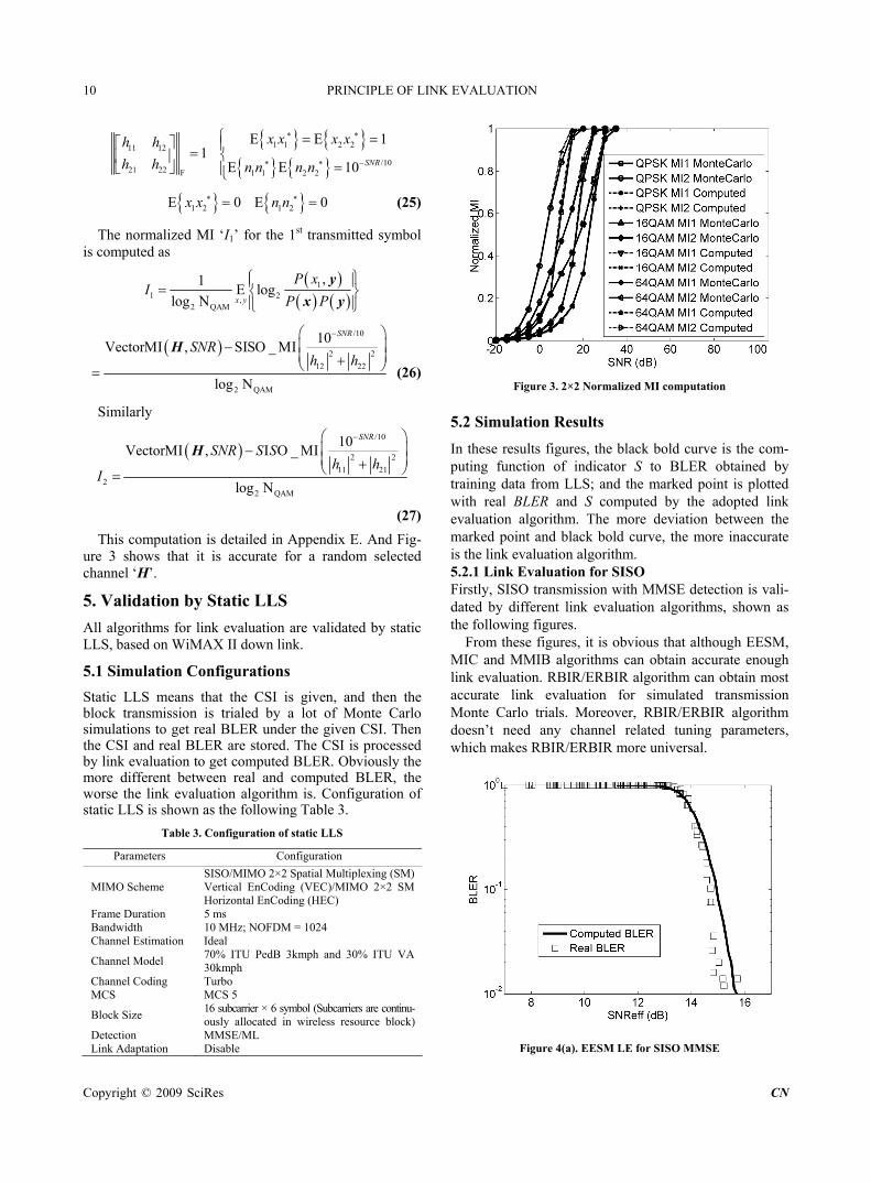
This computation is detailed in Appendix E. And Fig-ure 3 shows that it is accurate for a random selected channel ‘H’.

5. Validation by Static LLS

All algorithms for link evaluation are validated by static LLS, based on WiMAX II down link.

5.1 Simulation Configurations

St CSI is given, and then the block transmission is trialed by a lot of Monte Carlo simulations to get real BLER under the given CSI. Then the CSI and real BLER are stored. The CSI is processed by link evaluation to get computed BLER. Obviously t more different between real and computed BLER, the worse the link evaluation algorithm is. Configuratiostat

Configuration

atic LLS means that the

he

n of ic LLS is shown as the following Table 3.

Table 3. Configuration of static LLS

Parameters

MIMO Scheme SISO/MIMO 2×2 SVertical EnCoding

patial Multiplexing (SM) (VEC)/MIMO 2×2 SM

Horizontal EnCoding (HEC) Frame Duration 5 ms Bandwidth 10 MHz; NOFDM = 1024

mph and 30% ITU VA Channel Estimation Ideal

Channel Model 70% ITU PedB 3k30kmph

Channel Coding Turbo MCS MCS 5

Block Size 16 subcarrier × 6 symbol (Subcarriers are continu-ously allocated in wireless resource block)

Detection MMSE/ML Link Adaptation Disable

mputation Figure 3. 2

5.2 Simulation Results

In these results figures, the black bold curve is the com-puting function of indicator S to BLER obtained by training data from LLS; and the marked point is plotted with real BLER and S computed by the adopted link evaluation algorithm. The more deviation between the marked point and black bold curve, the more inaccurate is the link evaluation algorithm. 5.2.1 Link Evaluation for SISO Firstly, SISO transmission with MMSE detection is vali-dated by different link evaluation algorithms, shown as the following figures.

From these figures, it is obvious that although EESM, MIC and MMIB algorithms can obtain accurate eno

k evalu tain most for simulated transmission

ver, RBIR/ERBIR algorithm

×2 Normalized MI co

ugh lina

ation. RBIR/ERBIR algorithm can obccurate link evaluation

Monte Carlo trials. Moreodoesn’t need any channel related tuning parameters, which makes RBIR/ERBIR more universal.

Figure 4(a). EESM LE for SISO MMSE




Figure 4(b). MIC LE for SISO MMSE

Figure 5(a). MIC LE for SISO ML

Figu SE Figure 5(b). MMIB LE for SISO ML

re 4(c). RBIR/ERBIR LE for SISO MM

Figure 5(c). ERBIR LE for SISO ML

From thes and RBIR

algorithm is invalid, and MIC algorithm sho s too much accuracy. MMIB and ERBIR are of accurate enough

Figure 4(d). MMIB LE for SISO MMSE

Then, SISO transmission with ML detection is vali-

ated by different link evaluation algorithms, shown as the following figures.

e figures, it is obvious that EESMwd

in



Figure 6(a). EESM LE for VEC MMSE Figure 6(b). MIC LE for VEC MMSE

Figure 6(c). RBIR/ERBIR LE for VEC MMSE Figure 6(d). MMIB LE for VEC MMSE

results, while ERBIR is a bit better than MMIB. Here simulation results also validate the theoretical

conclusions. MIC chooses the upper bound of SER, so all the real BLER are bigger than computed BLER. And MMIB uses approximation in MI computation, so there is a little inaccuracy. 5.2.2 Link Evaluation for VEC Firstly, VEC transmission with MMSE detection is vali-dated by different link evaluation algorithms, shown as the following figures.

These figures show that although EESM, MIC anMIB algorithms can also obtain quite accurate link

evaluation, RBIoreover, RBIR/ERBIR algorithm doesn’t need any

nel related tuning parameters. Then, VEC transmission with ML detection is vali-

dated by different link evaluation algorithms, shown as

the following figures. Figure 7(a), Figure 7(b) and Figure 7(c) show that

EESM and RBIR algorithms are invalid, and MIC and MMIB algorithms show too much inaccuracy. ERBIR algorithm betters the accuracy of link evaluation for VEC ML transmissions a lot, although there is still some in-accuracy.

Here, MIC algorithm only provides the upper bound of wireless transmissions, and it is of the worst accuracy. Although MMIB seems a little better, for the sake of lim-

ed parameters presented in reference [7], the RBIRnot very accurate, so MMIB shows worse results than

5.2.3 Link Evaluation for HEC Firstly, HEC transmission with MMSE detection is vali-dated by different link evaluation algorithms, shown as the following figures.

d it is M

R/ERBIR algorithm is the most accurate. ERBIR. Mchan


Figure 7(a). MIC LE for VEC ML Figure 8(a). EESM LE for HEC MMSE

E Figure 7(b). MMIB LE for VEC ML

MS Figure 8(b). MIC LE for HEC M

Figure 8(c). RBIR/ERBIR LE for HEC MMSE

Figure 7(c). ERBIR LE for VEC ML




Figure 8(d). MMIB LE for HEC MMSE

These figures show that although EESM, MIC and

MMIB algorithms can also obtain quite accurate link evaluation, RBIR/ERBIR algorithm is the most accurate. Moreover, RBIR/ERBIR algorithm doesn’t need any channel related tuning parameters.

Then, HEC transmission with ML detection is vali-thms, shown as

dated by different link evaluation algori the following figures.

Figure 9 shows that EESM, RBIR, MIC and MMIB algorithms are invalid at all. Only ERBIR algorithm can achieve link evaluation for HEC ML transmissions.

5.3 Further Results Comparisons and Analysis

To ensure the universality of the simulation, more MCS levels are simulated. Following configuration in Table 3, MCS levels are set to MCS 1~8 with different MIMO schemes respectively. And the average difference is listed in the following tables. The average difference is measured by Mean Square Error Root (MSER) between computed and real BLER values.

Table 4. MSER for EESM li

Figure 9. ERBIR LE for HEC ML

nk evaluation MSE Transmission

Mode EESM MIC RBIR MMIB ERBIR

SISO with MMSEDetection

0.0369 0.1295 0. 0247 0. 0400 0. 0247

SISO with ML Detection

Not Supported

0.1296 Not

Supported 0. 0469 0. 0241

VEC with MMSEDetection

0. 0604

VEC with MLDetection Supported orted

0. 1 0956

H MMSEDetection

0.0256

HEC with D d S

ot ported

0.0547 0.1348 0. 0604 0. 0622

Not 0.3956

Not Supp

574 0.

EC with0. 0206 0851 0. 0. 0312 0.0206

ML Not etection Supporte

Not Nupported Sup

Not 0.0791

Supported

As to EESM quite a uation for nsmissions with MM on, o can not rios. T em, and MMIB are developed. Unfortunately, they are n ls either.

d MM t ters, wh es not. This makes E MIB iversal. RBIR is the most c gorithm for lf SE only. ERBI all scenarios.

lts in T -v accurate link nd more universality. M CS and lated tuning parameters are n r necessary, whv d accurate meth evaluation.

6. Validation by Link Adaptation and SLS

Link re v d S MAX II do ence caused by inaccuracy of link evaluation. Since previous results show that ERBIR is accurate, and MIC is not, link adaptation and SLS with ERBIR and MIC link evalua-tions are implemented.

6.1 Validation by Link Adaptation

Basic configuration of dynamical LLS is the same as Table 2, with link adaptation enable, 2×2 Alamouti STBC and MIMO 2×2 SM VEC of all MCS levels adap-tation, and ML detection. Receiver dynamically esti-mates the statistical performance of wireless channel, and chooses the MCS level which can get best Spectrum Ef-ficiency (SE) and acceptable BLER, then feeds it back to the transmitter [1].

Let target BL 10 15 20] dB. irstly Hybrid Au est (HARQ) is

and RBIR, although they have achievedccurate link eval

SE detecti wireless tra

because the computation is based support ML detection scenan OSINR, they

o solve this probl MIC ot accurate for some leve

EESM, MIC an IB need MCS and CSI relatedile RBIR douning parame

ESM, MIC and M not unommon alor MM

ink evaluation, but it can be used R can support link evaluation for

Simulation resu able 4 show that ERBIR can proluation aide more eva

oreover, the M CSI reo longeersal an

ich makes ERBIR become a uni-od for link

evaluations a alidated by link adaptation anLS of Wi wn link, profiling the influ

ER is 0.1, SNR is [5 tomatic Repeat reQuF

disabled, and simulation results are listed in the follow-ing Table 5.


Table 5. Dynamical LLS results without HARQ

Extended MI MIC

BLER [0.0334, 0.0125, 0.0052, 0.047]

[0.1545, 0.1482, 0.19, 0.2495]

Throughput (103 bits) [0.721, 1.111, 2.007, 3.093]

[0.687, 1.082, 1.819, 2.652]

Total Retransmission Times

[0 0 0 0] [0 0 0 0]

Then enable HARQ with maximum retransmission times of 3. Simulation results are listed in the following Table 6.

Compare the results of link adaptation with/without HARQ, it is obvious that accurate ERBIR link evaluation will ensure wireless system to choose proper MCS level, obtaining better BLER and throughput, and reducing the retransmission times. While using inaccurate MIC link evaluation, it is shown that MIC will overestimate the

in simulation results in pre-nd retransmission time

will become

mical LLS results with HARQ Extended MI MIC

link performance, as shownvious section. So BLER a s in-crease, and throughput decreases.

6.2 Validation by SLS

Configuration of dynamical SLS is listed in Table 6. In SLS, link evaluation is used to hold down real coding and decoding procedures, reducing SLS complexity, as described in Reference [1]. Because the BLER in SLS is computed by link evaluation, the SLS results

Table 6. Dyna

BLER [0 0 0 0] [0 0 0 0]

Throughput (103 bits) [0.747, 1.382, 2.294, 3.476]

[0.725, 1.166, 2.023, 3.245]

[13, 5, 3, 9] [53, 86, 46, 53] Total Retransmission Times

Table 7. Configuration of SLS figuration Parameters Con

MIMO Scheme Single user, 2×2 Alamouti STBC and MIMO 2×2 SM VEC Adaptation

Frame Duration 5 ms Bandwidth Channel Estimation

AM 2/3; 64QAM 3/4; 64QAM 5/6;

Block Size

DLi

H

C

Scheduling Proportional Fairness Scheduling

10 MHz; NOFDM = 1024 ideal

Channel Model 70% ITU PedB 3kmph and 30% ITU VA 30kmph

Channel Coding Turbo

MCS QPSK 1/2; QPSK 3/4; 16QAM 1/2; 16QAM 3/4; 64QAM 1/2; 64Q

16 subcarrier×6 symbol (Subcarriers are continuously allocated in wireless re-source block)

etection ML nk Adaptation Enable

Enable, with maximum retransmission ARQ

times of 3 Target BLER 0.1 Link Evaluation ERBIR/MIC

ell Configuration 3 sectors; omni directional antenna; 10 users per sector; 1.5 km of Cell Radius.

Figure 10. CDF of SLS SE

inaccurate when link evaluation can not provide accurate BLER.

Figure 10 shows the Cumulative Distribution Function

SLS results.

that RBIR is the most accurate metric, and a method to compute RBIR from CSI is proposed. Simulation results of LLS and SLS s works ve e prob-lem n

8. Acknowledgments

Tha n Zhen i, Zheng Hon ing, and Chen Yue

This work is sand developmenNa

[1] IEEE 802.16 Broadband Wireless Access Working Group. Draft IEEE 802.16m Evaluation Methodology Document. http:// ieee802.org/16/.July 18th, 2008.

[2] HE X, NIU K, HE Z Q, et al. Link layer abstraction in MIMO-OFDM system. International Workshop on Cross Layer De-sign, IWCLD’07, Sept. 20-21, 2007: 41-44.

[3] AKYILDIZ F, LEE W Y, AND VURAN M C, et al. A survey on spectrum management in cognitive radio networks. IEEE Communication Magazine, Apr. 2008, 46(4): 40-48.

[4] 3GPP TSG-RAN-1 Meeting #35, Effective SIR Computation for

(CDF) of SLS SE results. It is shown that the SLS SE is overestimated by MIC link evaluation by (2.0985 − 1.9075) / 1.9075 × 100% ≈ 10%. It is obvious that inac-curate link evaluation will lead to incredible

7. Conclusions

Link evaluation aims to provide a fading insensitive per-formance metric for common transmissions. It is proven from the view of information theory

how that the proposed ERBIR algorithmry well for common transmissions, solving th

s existing in current link evaluatio s.

nks to Ta hu gmyun for their great support.

upported in part by the Hi-tech research t program of China (2007AA01Z277),

tional Natural Science Foundation of China (6077 2035), University Doctorial Foundation of China (2007 0004010), and Intel China Research Centre.

REFERENCES




OFDM System-Level Simulations.

[5] WiMAX Forum. Mobile WiMAX-Part I: A Technical Ov -view and Performance Evaluation. white paper, August 2006.

[6] Ericsson. A Fading-Insensitive Performance Metric for a Unified

[7]

http://ieee802.org/16/. May 2nd, 2008.

[8] PAtio

[9] t detec-cations.

[10 A mathematical theory of communication. The ical Journal, July, October, 1948, 27: 379-423,

623-656.

[11] LEE J. W, BLAHUT R. E. Generalized EXIT chart analysis of finite-length turbo codes. Global TelecommConference, Dec. 2003, 4(1-5): 2067-2072.

1. Ef

The original wireless transmission is

y c I I ; ExIxIH = I(NS);

EnnH = σ2I(NR)

out interference symbol but the correlation, and H is consisted of corre-lated GaussiaGaussians.

H H

xx H = I(NS); E n1 n1 H = I(NR)

(31)

y = (T

σe2 = 1 / ||T−1HcF|| F (33)

This idenview of capacity. Let |A| means the determinant of matrix A. Ch f the original transmission is

C1 = log2|πeE H|

86-88, 178-198.

er CHUL H K, SUNGWOO P, MOON J, et al. Iterative jointion and decoding for MIMO-OFDM wireless communiFortieth Asilomar Conference on Signals, Systems and Com-puters, ACSSC’06. Oct.-Nov. 2006, 1752-1756.

Link Quality Model. ] SHANNON C. E.

Bell System Techn SAYANA K, ZHUANG J. Link performance abstraction based on mean mutual information per bit (MMIB) of the LLR channel.

and BER unication ULRAJ A. Introduction to space-time wireless communica-

ns. 1st Edition. Cambridge University Press, England, 2003:

APPENDIX

2

2 2log

H FF H R I

R I

c c R

R

fective MIMO Transmission

11 2R

2 11 2 HR

logT H FF H R I T

T R I T

H

c c

= H Fx + H x + n; ExxH = I(NS)

(28) = log2|I(NR) + (T−1HcF)(T−1HcF) H| (34)

ransmission is

C2 = log2|I(NR) + (T−1HcF)(T−1HcF) H| (35)

Equation (34) and (35) indicates that the two transmis-sions are effective.

2. OSINR Computation for MMSE

Consider transmission as

y = Hex + ne; Exx H = I(NS); E nene H = σe

2I(NR) (36)

Let xo = My = M(Hex +

Because receiver knows nothing abThen the channel capacity of the effective t

I

ns, HIxI + n is approximated as correlated Assume RI is known to the receiver.

E( HIxI + n)( HIxI + n) H = RI + σ2I(NR) (29)

Let En1n1 H = I(NR), and TT H = RI + σ2I(NR). So

E(Tn1)(Tn1) = E(HIxI + n)(HIxI + n) (30)

This means Tn1 is effective to HIxI + n, so the originalwireless transmission is effective to

y = HcFx + Tn1; E ne), where

2

o Far

MConsider identical transform, it is effective to

−1HcFx + n1) / ||T−1HcF||F = Hex + ne (32)

Where

He = T−1HcF / || T−1HcF|| F; Enene H = σe

2I(NR);

tity between (28) and (33) is proven from the

annel capacity o

yyH )(| − log2|πeE( HIxI + n HIxI + n)

g minM x x (37)

According to orthogonality principle,

E(xo − x) y H = 0 (38)

So, M = HeH(HeHe

H + σe2I)−1 (39)

Let, D = diag(MHe), N = diag(σe2MMH) and I =

MHe−D, then OSINR for each symbol in the transmitting signal vector is

γi = (DDH) ii / [(If If H) ii + (N) ii]; i = 1, 2, …, NS

eans the ith row and ith column element of ma-trix A.

3. Proof of Lemma 1

A LER is one-one to RBIR. Then consider the uncoded block

f

(40)

(A) ii m

2log

H F H x n H Fx H x n

c cx

ccording to Equation (20) and (21), BH x n H x n

, there is


BLERu = RBIRtoBLER(RBIRu) (41)

Since the MCS is given, it is pointed out that Extrinsic Information Transfer (EXIT) is definite [11]. So RBIR for the coded block after iterative decoding is determined by

RBIR = EXITMCS(RBIRu) (42)

So there is

BLER = RBIRtoBLER(RBIR) = RBIRtoBLER[E

=RBIRtoBLEREXITMCS[InversRBIRtoBLER(BLERu)] appingFunctionMCS(BLERu) (43)

This is referred to lemma 1.

4. Normalized MI for SISO

d symbol is

* = σ2 = 10−SNR/10 (44)

I is computed as

XITMCS(RBIRu)]

= M

For SISO transmission, the receive

y = Hx + n; Exx* = 1; Enn

2,

2 Q 2 Q

|1log

logI

log

x y

P y x MI

P y (45)

Since x is random selected from the constellation, t

P(x=qi)=1/NQAM

Where qi is the ith mapping point in the modulation co points in the co

hen

(46)

nstellation, and NQAM is the number ofnstellation. So

Q Q

2 Q1 1

Q

Then co

log | /

i kyi i

P y q P

MI (47)

nsider the probability of P(y | x),

|y q

| P y x P n y Hx

real imagreal imag P n y Hx P n y Hx

22

imagreal

2 2

1 1exp exp

y Hxy Hx

2

(48)

Let Δi,k = qi − qk,

2

1exp

y Hx

QΑΜ

QΑΜ

2

QΑΜ 2

2 21

,

21

QΑΜ

exp

log

exp

dn

i n i k

i

n

p nH n

MI

(49)

Here

2 2 2( ) exp( / ) /p n n

2 2 2

(50)

Let ne = n/H, and σe = σ /|H| then

2 2 2e e e( ) exp( / ) /p n n e (51)

So

QΑΜ

QΑΜ

2

eQΑΜ 2

e

e 2 21

, e

21

QΑΜ

exp

log

exp

i n i k

i

n

p n dnH n

MI

e

2/10SISO _ (10 / ) SNR H (52)

So

2/10

2 QΑΜ

1SISO _ (10 / )

log

SNRI H (53)

5. Normalized MI for 2×2 MIMO

2×2 MIMO received symbol is

1

2

1 11 12 1

2 21 22 2

Hx n

y h h xy

y h h x

n

n (54)

Where

1 1 2 2

2 /2 2

1 2 1 2

1

/ 10

0 0

SNR

x x x x

n

x x n n

1 1 n n n 10 (55)

For example, the normalized MI of x1 is

11 2,

2 QΑΜ

, |1log

log

y x

y

x y

P xI

P (56)

Since x1 and x2 are random selected from the constel-



lation,

P(x1 = q1,i, x2 = q2,j) = 1 / NQAM2 (57)

Here q1,i and q2,j are the ith and jth mapping points ithe constellation for x1 and x2 respectively. NQAM is the number of points in the constellation. Given transmitting vector,

ql = [q1,i, q2,j]T; l = 1,2,…,NQAM

2; i, j = 1,2,…,NQAM (58)

Let Δl,m = H(ql − qm),

n

2QΑΜ

2 21

12 2 2

QΑΜ

exp ( ) /q q n

mm

HP y

F

2

QΑΜ2

2

,1

2 2 4QΑΜ

exp /n

l mm

F

(59)

QΑΜ2

1, 1, 1 2

1 2, 2, 2

1, 2 4QΑΜ

exp /

, |

H

y q

i i

t j t

i l

q q n

q q nP q

F

QΑΜ 2

1 2

1 2, 2, 2

2 4QΑΜ

0exp /

t j t

nH

q q nF

(60)

Then

2QΑΜ

1,

21

1 2QΑΜ 2 QΑΜ

, |log

log

y qn n

y

i l

l n

p qp d

pI

2QΑΜ

1,

21

2QΑΜ 2 QΑΜ

, | /log

/

log

y q nn n

y n

i l

l n

p q pp d

p p

2

2QΑΜ

221QΑΜ 1,

2 QΑΜ

1log

log

nn n

l n

pp d

p q

, |y qi l

22 QΑΜ

1

log

cMI MI 1)

Consider MIc,

(6

QΑΜ

221QΑΜ

2 QΑΜ

1log

log

nn n

y

l n

pp d

p

2

QΑΜ1 nn

pc 22

1QΑΜ

logny

l n

MI p dp

2QΑΜ

2QΑΜ

221 2

,1

2QΑΜ

log

exp /

n n

n

l n

l mm

p d

F

22 2QΑΜ exp /n

F

2

QΑΜ

2QΑΜ

2QΑΜ

2 21

, , ,

21

2QΑΜ

log

exp

n nn n

H Hl n l m l m l m

m

p d

F

(62)

Let ne = (Δl,mHn+nHΔl,m) / || Δl,m||F, so

ne ~ N(0, 2σ2) (63)

Then

2

QΑΜ

2QΑΜ

2

e 2 21

, ,

21

2Q

log

exp

Q

l n l m l m e

m

c

p

ΑΜ

n dnn

MI

Then define approximation as

F F

2QΑΜ

2

,2e 2 2

1QΑΜ

1 1log exp

l m

lm

F ( 4)

Here the tuning parameter is

Table 8. Tuning parameter for 2×2 MIC

6




Then

2QΑΜ

222 2

1QΑΜ

log eVector ( , )H

c l

l

MI SNR (65)

Then compute MI2, and let Δ2,j,t = q2,j − q2,t,

QΑΜ QΑΜ

2 221 1 1QΑΜ

1 (( ) log

( , | )

nn n

y x

i j n

p )MI p

P x d

QΑΜ

2 2

1 22

2 21QΑΜ 12 2, , 1

exp1

( ) logn n

j n j t

n n

p dh n

QΑΜ2

22 2, , 2

21

exp

j t

t

h n( ) (66)

Here

2 2 2 2

12 2, , 1 22 2, , 2 12 22/ j t j th n h n h h( ) ( )

2 22 1 2 12 1 22 2

2, , 2, , real2 2 2 2

12 22 12 22

2

j t j t

n n h n h n

h h h h

(67)

Let ne = (h12n1* + h22n2

*) / (|h12|2 + |h22|

2), so

Ene = 0; Ene,realne,imag = 0; E|ne|2 = σe

2;

σe2 =σ2 / (|h12|

2 + |h22|2) (68)

Then

QΑΜ

QΑΜe

2

e2

e

2 e 2 21QΑΜ 2, , e

21 e

exp1

( ) log

exp(

j n j t

t

n

T p nn

)

edn

QΑΜ

QΑΜe

2

e2

e

2 e 2 21QΑΜ 2, , e

21 e

exp1

( ) log

exp(

j n j t

t

n

T p nn

)

edn

/10

2 2

12 22

10=SISO _

SNR

h h（） (69)

The computation of I1 and I2 are similar, so

/10

2 2

12 221

2 QΑΜ

10ector ( , ) _ )

log

H

SNR

SNRh h

I

V SISO (

/10

2 2

11 212

2 QΑΜ

10ector ( , ) SISO _ ( )

log

H

SNR

SNRh h

I

V

(70)

principle of link evaluation - semantic scholar

Documents