principal component analysis - sas · 2013-03-14 · principal component analysis is a variable...
TRANSCRIPT
1
Chapter 1
PRINCIPAL COMPONENT ANALYSIS
Introduction: The Basics of Principal Component Analysis . . . . . . . . . . . . . . . . . . . . . . . . . . . 2A Variable Reduction Procedure . . . . . . . . . . . . . . . . . . . . . . . . . . . . . . . . . . . . . . . . . . 2An Illustration of Variable Redundancy . . . . . . . . . . . . . . . . . . . . . . . . . . . . . . . . . . . . 3What is a Principal Component? . . . . . . . . . . . . . . . . . . . . . . . . . . . . . . . . . . . . . . . . . . 5
How principal components are computed . . . . . . . . . . . . . . . . . . . . . . . . . . . . . 5Number of components extracted . . . . . . . . . . . . . . . . . . . . . . . . . . . . . . . . . . . 7Characteristics of principal components . . . . . . . . . . . . . . . . . . . . . . . . . . . . . . 7
Orthogonal versus Oblique Solutions . . . . . . . . . . . . . . . . . . . . . . . . . . . . . . . . . . . . . . 8Principal Component Analysis is Not Factor Analysis . . . . . . . . . . . . . . . . . . . . . . . . . 9
Example: Analysis of the Prosocial Orientation Inventory . . . . . . . . . . . . . . . . . . . . . . . . . . 10Preparing a Multiple-Item Instrument . . . . . . . . . . . . . . . . . . . . . . . . . . . . . . . . . . . . . 11Number of Items per Component . . . . . . . . . . . . . . . . . . . . . . . . . . . . . . . . . . . . . . . . 12Minimally Adequate Sample Size . . . . . . . . . . . . . . . . . . . . . . . . . . . . . . . . . . . . . . . 13
SAS Program and Output . . . . . . . . . . . . . . . . . . . . . . . . . . . . . . . . . . . . . . . . . . . . . . . . . . . . . 13Writing the SAS Program . . . . . . . . . . . . . . . . . . . . . . . . . . . . . . . . . . . . . . . . . . . . . . 14
The DATA step . . . . . . . . . . . . . . . . . . . . . . . . . . . . . . . . . . . . . . . . . . . . . . . . 14The PROC FACTOR statement . . . . . . . . . . . . . . . . . . . . . . . . . . . . . . . . . . . . 15Options used with PROC FACTOR . . . . . . . . . . . . . . . . . . . . . . . . . . . . . . . . 15The VAR statement . . . . . . . . . . . . . . . . . . . . . . . . . . . . . . . . . . . . . . . . . . . . . 17Example of an actual program . . . . . . . . . . . . . . . . . . . . . . . . . . . . . . . . . . . . . 17
Results from the Output . . . . . . . . . . . . . . . . . . . . . . . . . . . . . . . . . . . . . . . . . . . . . . . . 17
Steps in Conducting Principal Component Analysis . . . . . . . . . . . . . . . . . . . . . . . . . . . . . . . . 21Step 1: Initial Extraction of the Components . . . . . . . . . . . . . . . . . . . . . . . . . . . . . . . 21Step 2: Determining the Number of “Meaningful” Components to Retain . . . . . . . . 22Step 3: Rotation to a Final Solution . . . . . . . . . . . . . . . . . . . . . . . . . . . . . . . . . . . . . . 28
Factor patterns and factor loadings . . . . . . . . . . . . . . . . . . . . . . . . . . . . . . . . . 28Rotations . . . . . . . . . . . . . . . . . . . . . . . . . . . . . . . . . . . . . . . . . . . . . . . . . . . . . 28
Step 4: Interpreting the Rotated Solution . . . . . . . . . . . . . . . . . . . . . . . . . . . . . . . . . . 28Step 5: Creating Factor Scores or Factor-Based Scores . . . . . . . . . . . . . . . . . . . . . . . 31
Computing factor scores . . . . . . . . . . . . . . . . . . . . . . . . . . . . . . . . . . . . . . . . . 32Computing factor-based scores . . . . . . . . . . . . . . . . . . . . . . . . . . . . . . . . . . . . 36Recoding reversed items prior to analysis . . . . . . . . . . . . . . . . . . . . . . . . . . . . 38
Step 6: Summarizing the Results in a Table . . . . . . . . . . . . . . . . . . . . . . . . . . . . . . . . 40Step 7: Preparing a Formal Description of the Results for a Paper . . . . . . . . . . . . . . 41

2 Principal Component Analysis
An Example with Three Retained Components . . . . . . . . . . . . . . . . . . . . . . . . . . . . . . . . . . . . 41The Questionnaire . . . . . . . . . . . . . . . . . . . . . . . . . . . . . . . . . . . . . . . . . . . . . . . . . . . . 41Writing the Program . . . . . . . . . . . . . . . . . . . . . . . . . . . . . . . . . . . . . . . . . . . . . . . . . . 43Results of the Initial Analysis . . . . . . . . . . . . . . . . . . . . . . . . . . . . . . . . . . . . . . . . . . . 44Results of the Second Analysis . . . . . . . . . . . . . . . . . . . . . . . . . . . . . . . . . . . . . . . . . . 50
Conclusion . . . . . . . . . . . . . . . . . . . . . . . . . . . . . . . . . . . . . . . . . . . . . . . . . . . . . . . . . . . . . . . . 55
Appendix: Assumptions Underlying Principal Component Analysis . . . . . . . . . . . . . . . . . . 55
References . . . . . . . . . . . . . . . . . . . . . . . . . . . . . . . . . . . . . . . . . . . . . . . . . . . . . . . . . . . . . . . . 56
Overview . This chapter provides an introduction to principal component analysis: avariable-reduction procedure similar to factor analysis. It provides guidelines regardingthe necessary sample size and number of items per component. It shows how to determinethe number of components to retain, interpret the rotated solution, create factor scores, andsummarize the results. Fictitious data from two studies are analyzed to illustrate theseprocedures. The present chapter deals only with the creation of orthogonal (uncorrelated)components; oblique (correlated) solutions are covered in Chapter 2, “Exploratory FactorAnalysis”.
Introduction: The Basics of Principal Component Analysis
Principal component analysis is appropriate when you have obtained measures on a number ofobserved variables and wish to develop a smaller number of artificial variables (called principalcomponents) that will account for most of the variance in the observed variables. The principalcomponents may then be used as predictor or criterion variables in subsequent analyses.
A Variable Reduction Procedure
Principal component analysis is a variable reduction procedure. It is useful when you haveobtained data on a number of variables (possibly a large number of variables), and believe thatthere is some redundancy in those variables. In this case, redundancy means that some of thevariables are correlated with one another, possibly because they are measuring the sameconstruct. Because of this redundancy, you believe that it should be possible to reduce theobserved variables into a smaller number of principal components (artificial variables) that willaccount for most of the variance in the observed variables.

Principal Component Analysis 3
Because it is a variable reduction procedure, principal component analysis is similar in manyrespects to exploratory factor analysis. In fact, the steps followed when conducting a principalcomponent analysis are virtually identical to those followed when conducting an exploratoryfactor analysis. However, there are significant conceptual differences between the twoprocedures, and it is important that you do not mistakenly claim that you are performing factoranalysis when you are actually performing principal component analysis. The differencesbetween these two procedures are described in greater detail in a later section titled “PrincipalComponent Analysis is Not Factor Analysis.”
An Illustration of Variable Redundancy
A specific (but fictitious) example of research will now be presented to illustrate the concept ofvariable redundancy introduced earlier. Imagine that you have developed a 7-item measure ofjob satisfaction. The instrument is reproduced here:
Please respond to each of the following statements by placing arating in the space to the left of the statement. In making yourratings, use any number from 1 to 7 in which 1=“strongly disagree”and 7=“strongly agree.”
_____ 1. My supervisor treats me with consideration._____ 2. My supervisor consults me concerning important decisions
that affect my work._____ 3. My supervisors give me recognition when I do a good job._____ 4. My supervisor gives me the support I need to do my job
well._____ 5. My pay is fair._____ 6. My pay is appropriate, given the amount of responsibility
that comes with my job._____ 7. My pay is comparable to the pay earned by other employees
whose jobs are similar to mine.
Perhaps you began your investigation with the intention of administering this questionnaire to200 or so employees, and using their responses to the seven items as seven separate variables insubsequent analyses (for example, perhaps you intended to use the seven items as seven separatepredictor variables in a multiple regression equation in which the criterion variable was“intention to quit the organization”).

4 Principal Component Analysis
There are a number of problems with conducting the study in this fashion, however. One of themore important problems involves the concept of redundancy that was mentioned earlier. Take aclose look at the content of the seven items in the questionnaire. Notice that items 1-4 all dealwith the same topic: the employees’ satisfaction with their supervisors. In this way, items 1-4are somewhat redundant to one another. Similarly, notice that items 5-7 also all seem to dealwith the same topic: the employees’ satisfaction with their pay.
Empirical findings may further support the notion that there is redundancy in the seven items. Assume that you administer the questionnaire to 200 employees and compute all possiblecorrelations between responses to the 7 items. The resulting fictitious correlations arereproduced in Table 1.1:
Table 1.1
Correlations among Seven Job Satisfaction Items_______________________________________________________
Correlations __________________________________________
Variable 1 2 3 4 5 6 7_______________________________________________________
1 1.00
2 .75 1.00
3 .83 .82 1.00
4 .68 .92 .88 1.00
5 .03 .01 .04 .01 1.00
6 .05 .02 .05 .07 .89 1.00
7 .02 .06 .00 .03 .91 .76 1.00__________________________________________________________________
Note : N = 200.
When correlations among several variables are computed, they are typically summarized in theform of a correlation matrix, such as the one reproduced in Table 1.1. This is an appropriateopportunity to review just how a correlation matrix is interpreted. The rows and columns of

Principal Component Analysis 5
Table 1.1 correspond to the seven variables included in the analysis: Row 1 (and column 1)represents variable 1, row 2 (and column 2) represents variable 2, and so forth. Where a givenrow and column intersect, you will find the correlation between the two corresponding variables. For example, where the row for variable 2 intersects with the column for variable 1, you find acorrelation of .75; this means that the correlation between variables 1 and 2 is .75.
The correlations of Table 1.1 show that the seven items seem to hang together in two distinctgroups. First, notice that items 1-4 show relatively strong correlations with one another. Thiscould be because items 1-4 are measuring the same construct. In the same way, items 5-7correlate strongly with one another (a possible indication that they all measure the sameconstruct as well). Even more interesting, notice that items 1-4 demonstrate very weakcorrelations with items 5-7. This is what you would expect to see if items 1-4 and items 5-7were measuring two different constructs.
Given this apparent redundancy, it is likely that the seven items of the questionnaire are notreally measuring seven different constructs; more likely, items 1-4 are measuring a singleconstruct that could reasonably be labelled “satisfaction with supervision,” while items 5-7 aremeasuring a different construct that could be labelled “satisfaction with pay.”
If responses to the seven items actually displayed the redundancy suggested by the pattern ofcorrelations in Table 1.1, it would be advantageous to somehow reduce the number of variablesin this data set, so that (in a sense) items 1-4 are collapsed into a single new variable that reflectsthe employees’ satisfaction with supervision, and items 5-7 are collapsed into a single newvariable that reflects satisfaction with pay. You could then use these two new artificial variables(rather than the seven original variables) as predictor variables in multiple regression, or in anyother type of analysis.
In essence, this is what is accomplished by principal component analysis: it allows you to reducea set of observed variables into a smaller set of artificial variables called principal components. The resulting principal components may then be used in subsequent analyses.
What is a Principal Component?
How principal components are computed. Technically, a principal component can bedefined as a linear combination of optimally-weighted observed variables. In order tounderstand the meaning of this definition, it is necessary to first describe how subject scores on aprincipal component are computed.
In the course of performing a principal component analysis, it is possible to calculate a score foreach subject on a given principal component. For example, in the preceding study, each subjectwould have scores on two components: one score on the satisfaction with supervisioncomponent, and one score on the satisfaction with pay component. The subject’s actual scoreson the seven questionnaire items would be optimally weighted and then summed to computetheir scores on a given component.

6 Principal Component Analysis
Below is the general form for the formula to compute scores on the first component extracted(created) in a principal component analysis:
C1 = b 11(X1) + b12(X 2) + ... b1p(Xp)
where
C1 = the subject’s score on principal component 1 (the first component extracted)
b1p = the regression coefficient (or weight) for observed variable p, as used increating principal component 1
Xp = the subject’s score on observed variable p.
For example, assume that component 1 in the present study was the “satisfaction withsupervision” component. You could determine each subject’s score on principal component 1 byusing the following fictitious formula:
C1 = .44 (X1) + .40 (X2) + .47 (X3) + .32 (X4) + .02 (X5) + .01 (X6) + .03 (X7)
In the present case, the observed variables (the “X” variables) were subject responses to theseven job satisfaction questions; X1 represents question 1, X2 represents question 2, and so forth.Notice that different regression coefficients were assigned to the different questions incomputing subject scores on component 1: Questions 1– 4 were assigned relatively largeregression weights that range from .32 to 44, while questions 5 –7 were assigned very smallweights ranging from .01 to .03. This makes sense, because component 1 is the satisfaction withsupervision component, and satisfaction with supervision was assessed by questions 1– 4. It istherefore appropriate that items 1– 4 would be given a good deal of weight in computing subjectscores on this component, while items 5 –7 would be given little weight.
Obviously, a different equation, with different regression weights, would be used to computesubject scores on component 2 (the satisfaction with pay component). Below is a fictitiousillustration of this formula:
C2 = .01 (X1) + .04 (X2) + .02 (X3) + .02 (X4) + .48 (X5) + .31 (X6) + .39 (X7)
The preceding shows that, in creating scores on the second component, much weight would begiven to items 5 –7, and little would be given to items 1– 4. As a result, component 2 should

Principal Component Analysis 7
account for much of the variability in the three satisfaction with pay items; that is, it should bestrongly correlated with those three items.
At this point, it is reasonable to wonder how the regression weights from the preceding equationsare determined. The SAS System’s PROC FACTOR solves for these weights by using a specialtype of equation called an eigenequation. The weights produced by these eigenequations areoptimal weights in the sense that, for a given set of data, no other set of weights could produce aset of components that are more successful in accounting for variance in the observed variables. The weights are created so as to satisfy a principle of least squares similar (but not identical) tothe principle of least squares used in multiple regression. Later, this chapter will show howPROC FACTOR can be used to extract (create) principal components.
It is now possible to better understand the definition that was offered at the beginning of thissection. There, a principal component was defined as a linear combination of optimallyweighted observed variables. The words “linear combination” refer to the fact that scores on acomponent are created by adding together scores on the observed variables being analyzed. “Optimally weighted” refers to the fact that the observed variables are weighted in such a waythat the resulting components account for a maximal amount of variance in the data set.
Number of components extracted . The preceding section may have created the impressionthat, if a principal component analysis were performed on data from the 7-item job satisfactionquestionnaire, only two components would be created. However, such an impression would notbe entirely correct.
In reality, the number of components extracted in a principal component analysis is equal to thenumber of observed variables being analyzed. This means that an analysis of your 7-itemquestionnaire would actually result in seven components, not two.
However, in most analyses, only the first few components account for meaningful amounts ofvariance, so only these first few components are retained, interpreted, and used in subsequentanalyses (such as in multiple regression analyses). For example, in your analysis of the 7-itemjob satisfaction questionnaire, it is likely that only the first two components would account for ameaningful amount of variance; therefore only these would be retained for interpretation. Youwould assume that the remaining five components accounted for only trivial amounts ofvariance. These latter components would therefore not be retained, interpreted, or furtheranalyzed.
Characteristics of principal components . The first component extracted in a principalcomponent analysis accounts for a maximal amount of total variance in the observed variables. Under typical conditions, this means that the first component will be correlated with at leastsome of the observed variables. It may be correlated with many.
The second component extracted will have two important characteristics. First, this componentwill account for a maximal amount of variance in the data set that was not accounted for by thefirst component. Again under typical conditions, this means that the second component will be

8 Principal Component Analysis
correlated with some of the observed variables that did not display strong correlations withcomponent 1.
The second characteristic of the second component is that it will be uncorrelated with the firstcomponent. Literally, if you were to compute the correlation between components 1 and 2, thatcorrelation would be zero.
The remaining components that are extracted in the analysis display the same two characteristics:each component accounts for a maximal amount of variance in the observed variables that wasnot accounted for by the preceding components, and is uncorrelated with all of the precedingcomponents. A principal component analysis proceeds in this fashion, with each new componentaccounting for progressively smaller and smaller amounts of variance (this is why only the firstfew components are usually retained and interpreted). When the analysis is complete, theresulting components will display varying degrees of correlation with the observed variables, butare completely uncorrelated with one another.
What is meant by “total variance” in the data set? To understand the meaning of “totalvariance” as it is used in a principal component analysis, remember that the observedvariables are standardized in the course of the analysis. This means that each variable istransformed so that it has a mean of zero and a variance of one. The “total variance” in thedata set is simply the sum of the variances of these observed variables. Because they havebeen standardized to have a variance of one, each observed variable contributes one unit ofvariance to the “total variance” in the data set. Because of this, the total variance in aprincipal component analysis will always be equal to the number of observed variablesbeing analyzed. For example, if seven variables are being analyzed, the total variance willequal seven. The components that are extracted in the analysis will partition this variance: perhaps the first component will account for 3.2 units of total variance; perhaps the secondcomponent will account for 2.1 units. The analysis continues in this way until all of thevariance in the data set has been accounted for.
Orthogonal versus Oblique Solutions
This chapter will discuss only principal component analyses that result in orthogonal solutions. An orthogonal solution is one in which the components remain uncorrelated (orthogonal means“uncorrelated”).
It is possible to perform a principal component analysis that results in correlated components. Such a solution is called an oblique solution . In some situations, oblique solutions are superiorto orthogonal solutions because they produce cleaner, more easily-interpreted results.
However, oblique solutions are also somewhat more complicated to interpret, compared toorthogonal solutions. For this reason, the present chapter will focus only on the interpretation of

Principal Component Analysis 9
orthogonal solutions. To learn about oblique solutions, see Chapter 2. The concepts discussed inthis chapter will provide a good foundation for the somewhat more complex concepts discussedin that chapter.
Principal Component Analysis is Not Factor Analysis
Principal component analysis is sometimes confused with factor analysis, and this isunderstandable, because there are many important similarities between the two procedures: bothare variable reduction methods that can be used to identify groups of observed variables that tendto hang together empirically. Both procedures can be performed with the SAS System’sFACTOR procedure, and they sometimes even provide very similar results.
Nonetheless, there are some important conceptual differences between principal componentanalysis and factor analysis that should be understood at the outset. Perhaps the most importantdeals with the assumption of an underlying causal structure: factor analysis assumes that thecovariation in the observed variables is due to the presence of one or more latent variables(factors) that exert causal influence on these observed variables. An example of such a causalstructure is presented in Figure 1.1:
V1
V2
V3
V4
Satisfactionwith
Supervision
SatisfactionwithPay
V5
V6
V7
Figure 1.1: Example of the Underlying Causal Structure that is Assumed in Factor Analysis
The ovals in Figure 1.1 represent the latent (unmeasured) factors of “satisfaction withsupervision” and “satisfaction with pay.” These factors are latent in the sense that they areassumed to actually exist in the employee’s belief systems, but cannot be measured directly. However, they do exert an influence on the employee’s responses to the seven items thatconstitute the job satisfaction questionnaire described earlier (these seven items are represented

10 Principal Component Analysis
as the squares labelled V1-V7 in the figure). It can be seen that the “supervision” factor exertsinfluence on items V1-V4 (the supervision questions), while the “pay” factor exerts influence onitems V5-V7 (the pay items).
Researchers use factor analysis when they believe that certain latent factors exist that exertcausal influence on the observed variables they are studying. Exploratory factor analysis helpsthe researcher identify the number and nature of these latent factors.
In contrast, principal component analysis makes no assumption about an underlying causalmodel. Principal component analysis is simply a variable reduction procedure that (typically)results in a relatively small number of components that account for most of the variance in a setof observed variables.
In summary, both factor analysis and principal component analysis have important roles to playin social science research, but their conceptual foundations are quite distinct.
Example: Analysis of the Prosocial Orientation Inventory
Assume that you have developed an instrument called the Prosocial Orientation Inventory (POI)that assesses the extent to which a person has engaged in helping behaviors over the precedingsix-month period. The instrument contains six items, and is reproduced here.
Instructions: Below are a number of activities that peoplesometimes engage in. For each item, please indicate howfrequently you have engaged in this activity over the precedingsix months. Make your rating by circling the appropriate numberto the left of the item, and use the following response format:
7 = Very Frequently 6 = Frequently 5 = Somewhat Frequently 4 = Occasionally 3 = Seldom 2 = Almost Never 1 = Never
1 2 3 4 5 6 7 1. Went out of my way to do a favor for acoworker.
1 2 3 4 5 6 7 2. Went out of my way to do a favor for arelative.

Principal Component Analysis 11
1 2 3 4 5 6 7 3. Went out of my way to do a favor for afriend.
1 2 3 4 5 6 7 4. Gave money to a religious charity.
1 2 3 4 5 6 7 5. Gave money to a charity not associated witha religion.
1 2 3 4 5 6 7 6. Gave money to a panhandler.
When you developed the instrument, you originally intended to administer it to a sample ofsubjects and use their responses to the six items as six separate predictor variables in a multipleregression equation. However, you have recently learned that this would be a questionablepractice (for the reasons discussed earlier), and have now decided to instead perform a principalcomponent analysis on responses to the six items to see if a smaller number of components cansuccessfully account for most of the variance in the data set. If this is the case, you will use theresulting components as the predictor variables in your multiple regression analyses.
At this point, it may be instructive to review the content of the six items that constitute the POI tomake an informed guess as to what you are likely to learn from the principal component analysis.Imagine that, when you first constructed the instrument, you assumed that the six items wereassessing six different types of prosocial behavior. However, inspection of items 1-3 shows thatthese three items share something in common: they all deal with the activity of “going out ofone’s way to do a favor for an acquaintance.” It would not be surprising to learn that these threeitems will hang together empirically in the principal component analysis to be performed. In thesame way, a review of items 4-6 shows that all of these items involve the activity of “givingmoney to the needy.” Again, it is possible that these three items will also group together in thecourse of the analysis.
In summary, the nature of the items suggests that it may be possible to account for the variancein the POI with just two components: An “acquaintance helping” component, and a “financialgiving” component. At this point, we are only speculating, of course; only a formal analysiscan tell us about the number and nature of the components measured by the POI.
(Remember that the preceding fictitious instrument is used for purposes of illustration only, andshould not be regarded as an example of a good measure of prosocial orientation; among otherproblems, this questionnaire obviously deals with very few forms of helping behavior).
Preparing a Multiple-Item Instrument
The preceding section illustrates an important point about how not to prepare a multiple-itemmeasure of a construct: Generally speaking, it is poor practice to throw together a questionnaire,administer it to a sample, and then perform a principal component analysis (or factor analysis) tosee what the questionnaire is measuring.

12 Principal Component Analysis
Better results are much more likely when you make a priori decisions about what you want thequestionnaire to measure, and then take steps to ensure that it does. For example, you wouldhave been more likely to obtain desirable results if you:
• had begun with a thorough review of theory and research on prosocial behavior
• used that review to determine how many types of prosocial behavior probably exist
• wrote multiple questionnaire items to assess each type of prosocial behavior.
Using this approach, you could have made statements such as “There are three types of prosocialbehavior: acquaintance helping, stranger helping, and financial giving.” You could have thenprepared a number of items to assess each of these three types, administered the questionnaire toa large sample, and performed a principal component analysis to see if the three components did,in fact, emerge.
Number of Items per Component
When a variable (such as a questionnaire item) is given a great deal of weight in constructing aprincipal component, we say that the variable loads on that component. For example, if the item“Went out of my way to do a favor for a coworker” is given a lot of weight in creating theacquaintance helping component, we say that this item loads on the acquaintance helpingcomponent.
It is highly desirable to have at least three (and preferably more) variables loading on eachretained component when the principal component analysis is complete. Because some of theitems may be dropped during the course of the analysis (for reasons to be discussed later), it isgenerally good practice to write at least five items for each construct that you wish to measure; inthis way, you increase the chances that at least three items per component will survive theanalysis. Note that we have unfortunately violated this recommendation by apparently writingonly three items for each of the two a priori components constituting the POI.
One additional note on scale length: the recommendation of three items per scale offered hereshould be viewed as an absolute minimum, and certainly not as an optimal number of items perscale. In practice, test and attitude scale developers normally desire that their scales containmany more than just three items to measure a given construct. It is not unusual to see individualscales that include 10, 20, or even more items to assess a single construct. Other things heldconstant, the more items in the scale, the more reliable it will be. The recommendation of threeitems per scale should therefore be viewed as a rock-bottom lower bound, appropriate only ifpractical concerns (such as total questionnaire length) prevent you from including more items. For more information on scale construction, see Spector (1992).

Principal Component Analysis 13
Minimally Adequate Sample Size
Principal component analysis is a large-sample procedure. To obtain reliable results, theminimal number of subjects providing usable data for the analysis should be the larger of 100subjects or five times the number of variables being analyzed.
To illustrate, assume that you wish to perform an analysis on responses to a 50-itemquestionnaire (remember that, when responses to a questionnaire are analyzed, the number ofvariables is equal to the number of items on the questionnaire). Five times the number of itemson the questionnaire equals 250. Therefore, your final sample should provide usable (complete)data from at least 250 subjects. It should be remembered, however, that any subject who fails toanswer just one item will not provide usable data for the principal component analysis, and willtherefore be dropped from the final sample. A certain number of subjects can always beexpected to leave at least one question blank (despite the most strongly worded instructions tothe contrary!). To ensure that the final sample includes at least 250 usable responses, you wouldbe wise to administer the questionnaire to perhaps 300-350 subjects.
These rules regarding the number of subjects per variable again constitute a lower bound, andsome have argued that they should apply only under two optimal conditions for principalcomponent analysis: when many variables are expected to load on each component, and whenvariable communalities are high. Under less optimal conditions, even larger samples may berequired.
What is a communality? A communality refers to the percent of variance in an observedvariable that is accounted for by the retained components (or factors). A given variablewill display a large communality if it loads heavily on at least one of the study’s retainedcomponents. Although communalities are computed in both procedures, the concept ofvariable communality is more relevant in a factor analysis than in principal componentanalysis.
SAS Program and Output
You may perform a principal component analysis using either the PRINCOMP or FACTORprocedures. This chapter will show how to perform the analysis using PROC FACTOR sincethis is a somewhat more flexible SAS System procedure (it is also possible to perform anexploratory factor analysis with PROC FACTOR). Because the analysis is to be performedusing the FACTOR procedure, the output will at times make references to factors rather than toprincipal components (i.e., component 1 will be referred to as FACTOR1 in the output,component 2 as FACTOR2, and so forth). However, it is important to remember that you arenonetheless performing a principal component analysis.

14 Principal Component Analysis
This section will provide instructions on writing the SAS program, along with an overview of theSAS output. A subsequent section will provide a more detailed treatment of the steps followedin the analysis, and the decisions to be made at each step.
Writing the SAS Program
The DATA step . To perform a principal component analysis, data may be input in the form ofraw data, a correlation matrix, a covariance matrix, as well as other some other types of data (fordetails, see Chapter 21 on “The FACTOR Procedure” in the SAS/STAT users guide, version 6,fourth edition, volume 1 [1989]). In this chapter’s first example, raw data will be analyzed.
Assume that you administered the POI to 50 subjects, and keyed their responses according to thefollowing keying guide:
VariableLine Column Name Explanation
1 1-6 V1-V6 Subjects’ responses to surveyquestions 1 through 6. Responses weremade using a 7-point “frequency”scale.
Here are the statements that will input these responses as raw data. The first three and the lastthree observations are reproduced here; for the entire data set, see Appendix B.
1 DATA D1; 2 INPUT #1 @1 (V1-V6) (1.) ; 3 CARDS; 4 556754 5 567343 6 777222 7 . 8 . 9 .10 76715111 45532312 45554413 ;
The data set in Appendix B includes only 50 cases so that it will be relatively easy for interestedreaders to key the data and replicate the analyses presented here. However, it should be

Principal Component Analysis 15
remembered that 50 observations will normally constitute an unacceptably small sample for aprincipal component analysis. Earlier it was said that a sample should provide usable data fromthe larger of either 100 cases or 5 times the number of observed variables. A small sample isbeing analyzed here for illustrative purposes only.
The PROC FACTOR statement . The general form for the SAS program to perform a principalcomponent analysis is presented here:
PROC FACTOR DATA=data-set-name SIMPLE METHOD=PRIN PRIORS=ONE MINEIGEN=p SCREE ROTATE=VARIMAX ROUND FLAG=desired-size-of-"significant"-factor-loadings ; VAR variables-to-be-analyzed ; RUN;
Options used with PROC FACTOR. The PROC FACTOR statement begins the FACTORprocedure, and a number of options may be requested in this statement before it ends with asemicolon. Some options that may be especially useful in social science research are:
FLAG=desired-size-of-”significant”-factor-loadings causes the printer to flag (with an asterisk) any factor loading whose absolute
value is greater than some specified size. For example, if you specify
FLAG=.35
an asterisk will appear next to any loading whose absolute value exceeds .35. Thisoption can make it much easier to interpret a factor pattern. Negative values arenot allowed in the FLAG option, and the FLAG option should be used inconjunction with the ROUND option.
METHOD=factor-extraction-method specifies the method to be used in extracting the factors or components. The
current program specifies METHOD=PRIN to request that the principal axis(principal factors) method be used for the initial extraction. This is the appropriatemethod for a principal component analysis.

16 Principal Component Analysis
MINEIGEN=p specifies the critical eigenvalue a component must display if that component is to
be retained (here, p = the critical eigenvalue). For example, the current programspecifies
MINEIGEN=1
This statement will cause PROC FACTOR to retain and rotate any componentwhose eigenvalue is 1.00 or larger. Negative values are not allowed.
NFACT=n allows you to specify the number of components to be retained and rotated, where
n = the number of components.
OUT=name-of-new-data-set creates a new data set that includes all of the variables of the existing data set,
along with factor scores for the components retained in the present analysis. Component 1 is given the varible name FACTOR1, component 2 is given thename FACTOR2, and so forth. It must be used in conjunction with the NFACToption, and the analysis must be based on raw data.
PRIORS=prior-communality-estimates specifies prior communality estimates. Users should always specify
PRIORS=ONE to perform a principal component analysis.
ROTATE=rotation-method specifies the rotation method to be used. The preceding program requests a
varimax rotation, which results in orthogonal (uncorrelated) components. Obliquerotations may also be requested; oblique rotations are discussed in Chapter 2.
ROUND causes all coefficients to be limited to two decimal places, rounded to the nearest
integer, and multiplied by 100 (thus eliminating the decimal point). This generallymakes it easier to read the coefficients because factor loadings and correlationcoefficients in the matrices printed by PROC FACTOR are normally carried out toseveral decimal places.
SCREE creates a plot that graphically displays the size of the eigenvalue associated with
each component. This can be used to perform a scree test to determine how manycomponents should be retained.
SIMPLE requests simple descriptive statistics: the number of usable cases on which the
analysis was performed, and the means and standard deviations of the observedvariables.
Principal Component Analysis 17
The VAR statement . The variables to be analyzed are listed in the VAR statement, with eachvariable separated by at least one space. Remember that the VAR statement is a separatestatement, not an option within the FACTOR statement, so don’t forget to end the FACTORstatement with a semicolon before beginning the VAR statement.
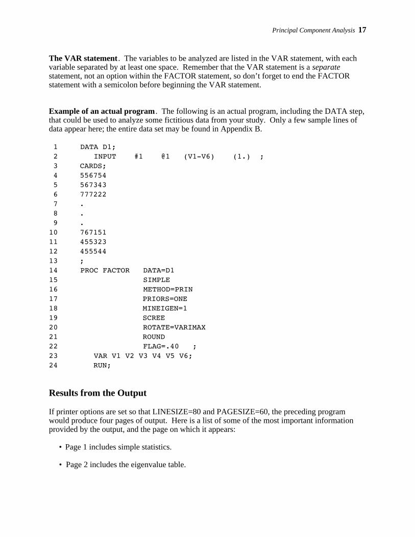
Example of an actual program . The following is an actual program, including the DATA step,that could be used to analyze some fictitious data from your study. Only a few sample lines ofdata appear here; the entire data set may be found in Appendix B.
1 DATA D1; 2 INPUT #1 @1 (V1-V6) (1.) ; 3 CARDS; 4 556754 5 567343 6 777222 7 . 8 . 9 .10 76715111 45532312 45554413 ;14 PROC FACTOR DATA=D115 SIMPLE 16 METHOD=PRIN17 PRIORS=ONE18 MINEIGEN=119 SCREE20 ROTATE=VARIMAX21 ROUND22 FLAG=.40 ;23 VAR V1 V2 V3 V4 V5 V6;24 RUN;
Results from the Output
If printer options are set so that LINESIZE=80 and PAGESIZE=60, the preceding programwould produce four pages of output. Here is a list of some of the most important informationprovided by the output, and the page on which it appears:
• Page 1 includes simple statistics.
• Page 2 includes the eigenvalue table.

18 Principal Component Analysis
• Page 3 includes the scree plot of eigenvalues.
• Page 4 includes the unrotated factor pattern and final communality estimates.
• Page 5 includes the rotated factor pattern.
The output created by the preceding program is reproduced here as Output 1.1:
The SAS System 1
Means and Standard Deviations from 50 observations
V1 V2 V3 V4 V5 V6Mean 5.18 5.4 5.52 3.64 4.22 3.1Std Dev 1.39518121 1.10656667 1.21621695 1.79295674 1.66953495 1.55511008
2
Initial Factor Method: Principal Components
Prior Communality Estimates: ONE
Eigenvalues of the Correlation Matrix: Total = 6 Average = 1
1 2 3 Eigenvalue 2.2664 1.9746 0.7973 Difference 0.2918 1.1773 0.3581 Proportion 0.3777 0.3291 0.1329 Cumulative 0.3777 0.7068 0.8397
4 5 6 Eigenvalue 0.4392 0.2913 0.2312 Difference 0.1479 0.0601 Proportion 0.0732 0.0485 0.0385 Cumulative 0.9129 0.9615 1.0000
2 factors will be retained by the MINEIGEN criterion.

Principal Component Analysis 19
3Initial Factor Method: Principal Components Scree Plot of Eigenvalues | | 2.25 + 1 | | | | 2.00 + | 2 | | | 1.75 + | | | | 1.50 + |E |i |g |e 1.25 +n |v |a |l |u 1.00 +e |s | | | 3 0.75 + | | | | 0.50 + | 4 | | | 5 0.25 + 6 | | | | 0.00 + | | ---------+--------+--------+--------+--------+--------+--------+--------- 0 1 2 3 4 5 6 Number
20 Principal Component Analysis
4
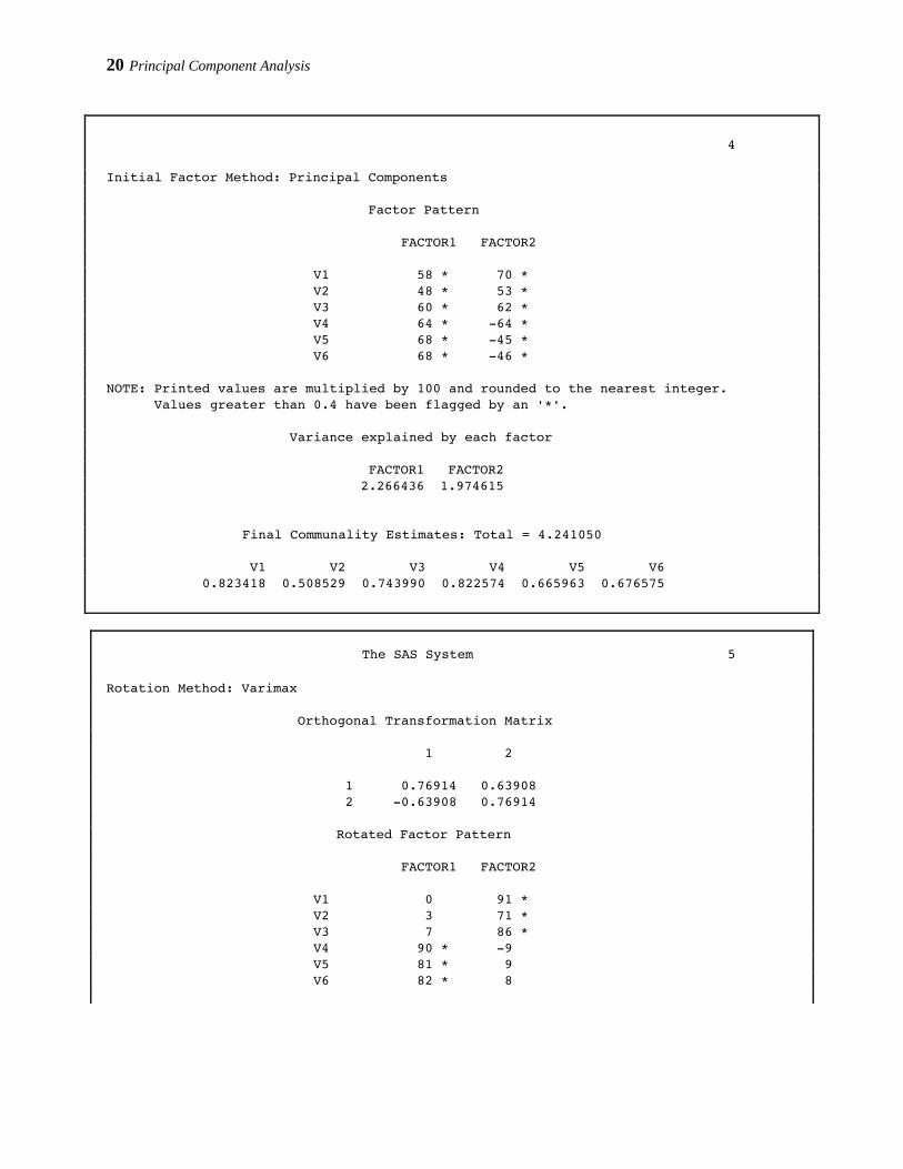
Initial Factor Method: Principal Components
Factor Pattern
FACTOR1 FACTOR2
V1 58 * 70 * V2 48 * 53 * V3 60 * 62 * V4 64 * -64 * V5 68 * -45 * V6 68 * -46 *
NOTE: Printed values are multiplied by 100 and rounded to the nearest integer. Values greater than 0.4 have been flagged by an '*'.
Variance explained by each factor
FACTOR1 FACTOR2 2.266436 1.974615
Final Communality Estimates: Total = 4.241050
V1 V2 V3 V4 V5 V6 0.823418 0.508529 0.743990 0.822574 0.665963 0.676575
The SAS System 5
Rotation Method: Varimax
Orthogonal Transformation Matrix
1 2
1 0.76914 0.63908 2 -0.63908 0.76914
Rotated Factor Pattern
FACTOR1 FACTOR2
V1 0 91 * V2 3 71 * V3 7 86 * V4 90 * -9 V5 81 * 9 V6 82 * 8

Principal Component Analysis 21
NOTE: Printed values are multiplied by 100 and rounded to the nearest integer. Values greater than 0.4 have been flagged by an '*'.
Variance explained by each factor
FACTOR1 FACTOR2 2.147248 2.093803
Final Communality Estimates: Total = 4.241050
V1 V2 V3 V4 V5 V6 0.823418 0.508529 0.743990 0.822574 0.665963 0.676575
Output 1.1: Results of the Initial Principal Component Analysis of the Prosocial OrientationInventory (POI) Data
Page 1 from Output 1.1 provides simple statistics for the observed variables included in theanalysis. Once the SAS log has been checked to verify that no errors were made in the analysis,these simple statistics should be reviewed to determine how many usable observations wereincluded in the analysis and to verify that the means and standard deviations are in the expectedrange. The top line of Output 1.1, page 1, says “Means and Standard Deviations from 50Observations”, meaning that data from 50 subjects were included in the analysis.
Steps in Conducting Principal Component Analysis
Principal component analysis is normally conducted in a sequence of steps, with somewhatsubjective decisions being made at many of these steps. Because this is an introductorytreatment of the topic, it will not provide a comprehensive discussion of all of the optionsavailable to you at each step. Instead, specific recommendations will be made, consistent withpractices often followed in applied research. For a more detailed treatment of principalcomponent analysis and its close relative, factor analysis, see Kim and Mueller (1978a; 1978b),Rummel (1970), or Stevens (1986).
Step 1: Initial Extraction of the Components
In principal component analysis, the number of components extracted is equal to the number ofvariables being analyzed. Because six variables are analyzed in the present study, sixcomponents will be extracted. The first component can be expected to account for a fairly largeamount of the total variance. Each succeeding component will account for progressively smalleramounts of variance. Although a large number of components may be extracted in this way,only the first few components will be important enough to be retained for interpretation.

22 Principal Component Analysis
Page 2 from Output 1.1 provides the eigenvalue table from the analysis (this table appears justbelow the heading “Eigenvalues of the Correlation Matrix: Total = 6 Average = 1”). Aneigenvalue represents the amount of variance that is accounted for by a given component. In therow headed “Eignenvalue” (running from left to right), the eigenvalue for each component ispresented. Each column in the matrix (running up and down) presents information about one ofthe six components: The column headed “1” provides information about the first componentextracted, the column headed “2” provides information about the second component extracted,and so forth.
Where the row headed EIGENVALUE intersects with the columns headed “1” and “2,” it can beseen that the eigenvalue for component 1 is 2.27, while the eigenvalue for component 2 is 1.97. This pattern is consistent with our earlier statement that the first components extracted tend toaccount for relatively large amounts of variance, while the later components account forrelatively smaller amounts.
Step 2: Determining the Number of “Meaningful” Components to Retain
Earlier it was stated that the number of components extracted is equal to the number of variablesbeing analyzed, necessitating that you decide just how many of these components are trulymeaningful and worthy of being retained for rotation and interpretation. In general, you expectthat only the first few components will account for meaningful amounts of variance, and that thelater components will tend to account for only trivial variance. The next step of the analysis,therefore, is to determine how many meaningful components should be retained forinterpretation. This section will describe four criteria that may be used in making this decision: the eigenvalue-one criterion, the scree test, the proportion of variance accounted for, and theinterpretability criterion.
A. The eigenvalue-one criterion. In principal component analysis, one of the most commonlyused criteria for solving the number-of-components problem is the eigenvalue-one criterion, alsoknown as the Kaiser criterion (Kaiser, 1960). With this approach, you retain and interpret anycomponent with an eigenvalue greater than 1.00.
The rationale for this criterion is straightforward. Each observed variable contributes one unit ofvariance to the total variance in the data set. Any component that displays an eigenvalue greaterthan 1.00 is accounting for a greater amount of variance than had been contributed by onevariable. Such a component is therefore accounting for a meaningful amount of variance, and isworthy of being retained.
On the other hand, a component with an eigenvalue less than 1.00 is accounting for less variancethan had been contributed by one variable. The purpose of principal component analysis is toreduce a number of observed variables into a relatively smaller number of components; thiscannot be effectively achieved if you retain components that account for less variance than hadbeen contributed by individual variables. For this reason, components with eigenvalues less than1.00 are viewed as trivial, and are not retained.

Principal Component Analysis 23
The eigenvalue-one criterion has a number of positive features that have contributed to itspopularity. Perhaps the most important reason for its widespread use is its simplicity: You donot make any subjective decisions, but merely retain components with eigenvalues greater thanone.
On the positive side, it has been shown that this criterion very often results in retaining thecorrect number of components, particularly when a small to moderate number of variables arebeing analyzed and the variable communalities are high. Stevens (1986) reviews studies thathave investigated the accuracy of the eigenvalue-one criterion, and recommends its use whenless than 30 variables are being analyzed and communalities are greater than .70, or when theanalysis is based on over 250 observations and the mean communality is greater than or equal to.60.
There are a number of problems associated with the eigenvalue-one criterion, however. As wassuggested in the preceding paragraph, it can lead to retaining the wrong number of componentsunder circumstances that are often encountered in research (e.g., when many variables areanalyzed, when communalities are small). Also, the mindless application of this criterion canlead to retaining a certain number of components when the actual difference in the eigenvaluesof successive components is only trivial. For example, if component 2 displays an eigenvalue of1.001 and component 3 displays an eigenvalue of 0.999, then component 2 will be retained butcomponent 3 will not; this may mislead you into believing that the third component wasmeaningless when, in fact, it accounted for almost exactly the same amount of variance as thesecond component. In short, the eigenvalue-one criterion can be helpful when used judiciously,but the thoughtless application of this approach can lead to serious errors of interpretation.
With the SAS System, the eigenvalue-one criterion can be implemented by including theMINEIGEN=1 option in the PROC FACTOR statement, and not including the NFACT option. The use of MINEIGEN=1 will cause PROC FACTOR to retain any component with aneigenvalue greater than 1.00.
The eigenvalue table from the current analysis appears on page 2 of Output 1.1. The eigenvaluesfor components 1, 2, and 3 were 2.27, 1.97, and 0.80, respectively. Only components 1 and 2demonstrated eigenvalues greater than 1.00, so the eigenvalue-one criterion would lead you toretain and interpret only these two components.
Fortunately, the application of the criterion is fairly unambiguous in this case: The lastcomponent retained (2) displays an eigenvalue of 1.97, which is substantially greater than 1.00,and the next component (3) displays an eigenvalue of 0.80, which is clearly lower than 1.00. Inthis analysis, you are not faced with the difficult decision of whether to retain a component thatdemonstrates an eigenvalue that is close to 1.00, but not quite there (e.g., an eigenvalue of .98). In situations such as this, the eigenvalue-one criterion may be used with greater confidence.
B. The scree test . With the scree test (Cattell, 1966), you plot the eigenvalues associated witheach component and look for a “break” between the components with relatively largeeigenvalues and those with small eigenvalues. The components that appear before the break areassumed to be meaningful and are retained for rotation; those apppearing after the break areassumed to be unimportant and are not retained.
24 Principal Component Analysis
Sometimes a scree plot will display several large breaks. When this is the case, you should lookfor the last big break before the eigenvalues begin to level off. Only the components that appearbefore this last large break should be retained.
Specifying the SCREE option in the PROC FACTOR statement causes the SAS System to printan eigenvalue plot as part of the output. This appears as page 3 of Output 1.1.
You can see that the component numbers are listed on the horizontal axis, while eigenvalues arelisted on the vertical axis. With this plot, notice that there is a relatively small break betweencomponent 1 and 2, and a relatively large break following component 2. The breaks betweencomponents 3, 4, 5, and 6 are all relatively small.
Because the large break in this plot appears between components 2 and 3, the scree test wouldlead you to retain only components 1 and 2. The components appearing after the break (3-6)would be regarded as trivial.
The scree test can be expected to provide reasonably accurate results, provided the sample islarge (over 200) and most of the variable communalities are large (Stevens, 1986). However,this criterion has its own weaknesses as well, most notably the ambiguity that is often displayedby scree plots under typical research conditions: Very often, it is difficult to determine exactlywhere in the scree plot a break exists, or even if a break exists at all.
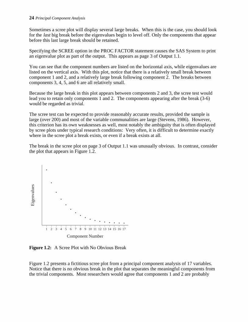
The break in the scree plot on page 3 of Output 1.1 was unusually obvious. In contrast, considerthe plot that appears in Figure 1.2.
Eig
enva
lues
Component Number
1 2 3 4 5 6 7 8 9 10 11 12 13 14 15 16 17
Figure 1.2: A Scree Plot with No Obvious Break
Figure 1.2 presents a fictitious scree plot from a principal component analysis of 17 variables. Notice that there is no obvious break in the plot that separates the meaningful components fromthe trivial components. Most researchers would agree that components 1 and 2 are probably
Principal Component Analysis 25
meaningful, and that components 13–17 are probably trivial, but it is difficult to decide exactlywhere you should draw the line.
Scree plots such as the one presented in Figure 1.2 are common in social science research. Whenencountered, the use of the scree test must be supplemented with additional criteria, such as thevariance accounted for criterion and the interpretability criterion, to be described later.
Why do they call it a “scree” test? The word “scree” refers to the loose rubble that lies atthe base of a cliff. When performing a scree test, you normally hope that the scree plotwill take the form of a cliff: At the top will be the eigenvalues for the few meaningfulcomponents, followed by a break (the edge of the cliff). At the bottom of the cliff will liethe scree: eigenvalues for the trivial components.
In some cases, a computer printer may not be able to prepare an eigenvalue plot with the degreeof precision that is necessary to perform a sensitive scree test. In such cases, it may be best toprepare the plot by hand. This may be done simply by referring to the eigenvalue table on outputpage 2. Using the eigenvalues from this table, you can prepare an eigenvalue plot following thesame format used by the SAS System (component numbers on the horizontal axis, eigenvalueson the vertical). Such a hand-drawn plot may make it easier to identify the break in theeigenvalues, if one exists.
C. Proportion of variance accounted for. A third criterion in solving the number of factorsproblem involves retaining a component if it accounts for a specified proportion (or percentage)of variance in the data set. For example, you may decide to retain any component that accountsfor at least 5% or 10% of the total variance. This proportion can be calculated with a simpleformula:
Proportion = Eigenvalue for the component of interest
Total eigenvalues of the correlation matrix
In principal component analysis, the “total eigenvalues of the correlation matrix” is equal to thetotal number of variables being analyzed (because each variable contributes one unit of varianceto the analysis).
Fortunately, it is not necessary to actually compute these percentages by hand, since they areprovided in the results of PROC FACTOR. The proportion of variance accounted for by eachcomponent is printed in the eigenvalue table from output page 2, and appears to the right of the“Proportion” heading.
The eigenvalue table for the current analysis appears on page 2 of Output 1.1. From the“Proportion” line in this eigenvalue table, you can see that the first component alone accounts for38% of the total variance, the second component alone accounts for 33%, the third component

26 Principal Component Analysis
accounts for 13%, and the fourth component accounts for 7%. Assume that you have decided toretain any component that accounts for at least 10% of the total variance in the data set. For thepresent results, using this criterion would cause you to retain components 1, 2, and 3 (notice thatuse of this criterion would result in retaining more components than would be retained with thetwo preceding criteria).
An alternative criterion is to retain enough components so that the cumulative percent of varianceaccounted for is equal to some minimal value. For example, remember that components 1, 2, 3,and 4 accounted for approximately 38%, 33%, 13%, and 7% of the total variance, respectively. Adding these percentages together results in a sum of 91%. This means that the cumulativepercent of variance accounted for by components 1, 2, 3, and 4 is 91%. When researchers usethe “cumulative percent of variance accounted for” as the criterion for solving the number-of-components problem, they usually retain enough components so that the cumulative percent ofvariance accounted for at least 70% (and sometimes 80%).
With respect to the results of PROC FACTOR, the “cumulative percent of variance accountedfor” is presented in the eigenvalue table (from page 2), to the right of the “Cumulative” heading.For the present analysis, this information appears in the eigenvalue table on page 2 of Output 1.1. Notice the values that appear to the right of the heading “Cumulative”: Each valuein this line indicates the percent of variance accounted for by the present component, as well asall preceding components. For example, the value for component 2 is .7068 (this appears at theintersection of the row headed “Cumulative” and the column headed “2”). This value of .7068indicates that approximately 71% of the total variance is accounted for by components 1 and 2combined. The corresponding entry for component 3 is .8397, meaning that approximately 84%of the variance is accounted for by components 1, 2, and 3 combined. If you were to use 70% asthe “critical value” for determining the number of components to retain, you would retaincomponents 1 and 2 in the present analysis.
The proportion of variance criterion has a number of positive features. For example, in mostcases, you would not want to retain a group of components that, combined, account for only a minority of the variance in the data set (say, 30%). Nonetheless, the critical values discussedearlier (10% for individual components and 70%-80% for the combined components) areobviously arbitrary. Because of these and related problems, this approach has sometimes beencriticized for its subjectivity (Kim & Mueller, 1978b).
D. The interpretability criteria. Perhaps the most important criterion for solving the “number-of-components” problem is the interpretability criterion: interpreting the substantive meaningof the retained components and verifying that this interpretation makes sense in terms of what isknown about the constructs under investigation. The following list provides four rules to followin doing this. A later section (titled “Step 4: Interpreting the Rotated Solution”) shows how toactually interpret the results of a principal component analysis; the following rules will be moremeaningful after you have completed that section.
1. Are there at least three variables (items) with significant loadings on each retainedcomponent? A solution is less satisfactory if a given component is measured by less thanthree variables.

Principal Component Analysis 27
2. Do the variables that load on a given component share the same conceptual meaning? For example, if three questions on a survey all load on component 1, do all three of thesequestions seem to be measuring the same construct?
3. Do the variables that load on different components seem to be measuring differentconstructs? For example, if three questions load on component 1, and three otherquestions load on component 2, do the first three questions seem to be measuring aconstruct that is conceptually different from the construct measured by the last threequestions?
4. Does the rotated factor pattern demonstrate “simple structure?” Simple structuremeans that the pattern possesses two characteristics: (a) Most of the variables haverelatively high factor loadings on only one component, and near zero loadings on the othercomponents, and (b) most components have relatively high factor loadings for somevariables, and near-zero loadings for the remaining variables. This concept of simplestructure will be explained in more detail in a later section titled “Step 4: Interpreting theRotated Solution.”
Recommendations . Given the preceding options, what procedure should you actually follow insolving the number-of-components problem? We recommend combining all four in a structuredsequence. First, use the MINEIGEN=1 options to implement the eigenvalue-one criterion. Review this solution for interpretability, and use caution if the break between the componentswith eigenvalues above 1.00 and those below 1.00 is not clear-cut (i.e., if component 2 has aneigenvalue of 1.001, and component 2 has an eigenvalue of 0.998).
Next, perform a scree test and look for obvious breaks in the eigenvalues. Because there willoften be more than one break in the scree plot, it may be necessary to examine two or morepossible solutions.
Next, review the amount of common variance accounted for by each individual component. Youprobably should not rigidly use some specific but arbitrary cutoff point such as 5% or 10%. Still,if you are retaining components that account for as little as 2% or 4% of the variance, it may bewise to take a second look at the solution and verify that these latter components are of trulysubstantive importance. In the same way, it is best if the combined components account for atleast 70% of the cumulative variance; if less than 70% is accounted for, it may be wise toconsider alternative solutions that include a larger number of components.
Finally, apply the interpretability criteria to each solution that is examined. If more than onesolution can be justified on the basis of the preceding criteria, which of these solutions is themost interpretable? By seeking a solution that is both interpretable and also satisfies one (ormore) of the other three criteria, you maximize chances of retaining the correct number ofcomponents.

28 Principal Component Analysis
Step 3: Rotation to a Final Solution
Factor patterns and factor loadings. After extracting the initial components, PROC FACTORwill create an unrotated factor pattern matrix. The rows of this matrix represent the variablesbeing analyzed, and the columns represent the retained components (these components arereferred to as FACTOR1, FACTOR2 and so forth in the output).
The entries in the matrix are factor loadings. A factor loading is a general term for a coefficientthat appears in a factor pattern matrix or a factor structure matrix. In an analysis that results inoblique (correlated) components, the definition for a factor loading is different depending onwhether it is in a factor pattern matrix or in a factor structure matrix. However, the situation issimpler in an analysis that results in orthogonal components (as in the present chapter): In anorthogonal analysis, factor loadings are equivalent to bivariate correlations between the observedvariables and the components.
For example, the factor pattern matrix from the current analysis appears on page 4 of Output 1.1. Where the rows for observed variables intersect with the column for FACTOR1, youcan see that the correlation between V1 and the first component is .58; the correlation betweenV2 and the first component is .48, and so forth.
Rotations. Ideally, you would like to review the correlations between the variables and thecomponents and use this information to interpret the components; that is, to determine whatconstruct seems to be measured by component 1, what construct seems to be measured bycomponent 2, and so forth. Unfortunately, when more than one component has been retained inan analysis, the interpretation of an unrotated factor pattern is usually quite difficult. To makeinterpretation easier, you will normally perform an operation called a rotation. A rotation is alinear transformation that is performed on the factor solution for the purpose of making thesolution easier to interpret.
PROC FACTOR allows you to request several different types of rotations. The precedingprogram that analyzed data from the POI study included the statement
ROTATE=VARIMAX
which requests a varimax rotation . A varimax rotation is an orthogonal rotation, meaning thatit results in uncorrelated components. Compared to some other types of rotations, a varimaxrotation tends to maximize the variance of a column of the factor pattern matrix (as opposed to arow of the matrix). This rotation is probably the most commonly used orthogonal rotation in thesocial sciences. The results of the varimax rotation for the current analysis appear on page 5 ofOutput 1.1.
Step 4: Interpreting the Rotated Solution
Interpreting a rotated solution means determining just what is measured by each of the retainedcomponents. Briefly, this involves identifying the variables that demonstrate high loadings for a

Principal Component Analysis 29
given component, and determining what these variables have in common. Usually, a brief nameis assigned to each retained component that describes its content.
The first decision to be made at this stage is to decide how large a factor loading must be to beconsidered “large.” Stevens (1986) discusses some of the issues relevant to this decision, andeven provides guidelines for testing the statistical significance of factor loadings. Given that thisis an introductory treatment of principal component analysis, however, simply consider a loadingto be “large” if its absolute value exceeds .40.
The rotated factor pattern for the POI study appears on page 5 of Output 1.1. The following textprovides a structured approach for interpreting this factor pattern.
A. Read across the row for the first variable . All “meaningful loadings” (i.e., loadingsgreater than .40) have been flagged with an asterisk (“*”). This was accomplished by includingthe FLAG=.40 option in the preceding program. If a given variable has a meaningful loading onmore than one component, scratch that variable out and ignore it in your interpretation. In manysituations, researchers want to drop variables that load on more than one component, because thevariables are not pure measures of any one construct. In the present case, this means looking atthe row headed “V1”, and reading to the right to see if it loads on more than one component. Inthis case it does not, so you may retain this variable.
B. Repeat this process for the remaining variables, scratching out any variable that loadson more than one component. In this analysis, none of the variables have high loadings onmore than one component, so none will have to be dropped.
C. Review all of the surviving variables with high loadings on component 1 to determinethe nature of this component. From the rotated factor pattern, you can see that only items 4, 5,and 6 load on component 1 (note the asterisks). It is now necessary to turn to the questionnaireitself and review the content of the questions in order to decide what a given component shouldbe named. What do questions 4, 5, and 6 have in common? What common construct do theyseem to be measuring? For illustration, the questions being analyzed in the present case arereproduced here. Remember that question 4 was represented as V4 in the SAS program,question 5 was V5, and so forth. Read questions 4, 5, and 6 to see what they have in common.
1 2 3 4 5 6 7 1. Went out of my way to do a favor for acoworker.
1 2 3 4 5 6 7 2. Went out of my way to do a favor for arelative.
1 2 3 4 5 6 7 3. Went out of my way to do a favor for afriend.

30 Principal Component Analysis
1 2 3 4 5 6 7 4. Gave money to a religious charity.
1 2 3 4 5 6 7 5. Gave money to a charity not associated with areligion.
1 2 3 4 5 6 7 6. Gave money to a panhandler.
Questions 4, 5, and 6 all seem to deal with “giving money to the needy.” It is thereforereasonable to label component 1 the “financial giving” component.
D. Repeat this process to name the remaining retained components. In the present case,there is only one remaining component to name: component 2. This component has highloadings for questions 1, 2, and 3. In reviewing these items, it becomes clear that each seems todeal with helping friends, relatives, or other acquaintances. It is therefore appropriate to namethis the “acquaintance helping” component.
E. Determine whether this final solution satisfies the interpretability criteria. An earliersection indicated that the overall results of a principal component analysis are satisfactory only ifthey meet a number of interpretability criteria. In the following list, the adequacy of the rotatedfactor pattern presented on page 5 of Output 1.1 is assessed in terms of these criteria.
1. Are there at least three variables (items) with significant loadings on each retainedcomponent? In the present example, three variables loaded on component 1, and threealso loaded on component 2, so this criterion was met.
2. Do the variables that load on a given component share some conceptual meaning? All three variables loading on component 1 are clearly measuring giving to the needy,while all three loading on component 2 are clearly measuring prosocial acts performedfor acquaintances. Therefore, this criterion is met.
3. Do the variables that load on different components seem to be measuring differentconstructs? The items loading on component 1 clearly are measuring the respondents’financial contributions, while the items loading on component 2 are clearly measuringhelpfulness toward acquaintances. Because these seem to be conceptually very differentconstructs, this criterion seems to be met as well.
4. Does the rotated factor pattern demonstrate “simple structure?” Earlier, it was saidthat a rotated factor pattern demonstrates simple structure when it has twocharacteristics. First, most of the variables should have high loadings on onecomponent, and near-zero loadings on the other components. It can be seen that thepattern obtained here meets that requirement: items 1-3 have high loadings on

Principal Component Analysis 31
component 2, and near-zero loadings on component 1. Similarly, items 4-6 have highloadings on component 1, and near-zero loadings on component 2. The secondcharacteristic of simple structure is that each component should have high loadings forsome variables, and near-zero loadings for the others. Again, the pattern obtained herealso meets this requirement: component 1 has high loadings for items 4-6 and near-zeroloadings for the other items, while component 2 has high loadings for items 1-3, andnear-zero loadings on the remaining items. In short, the rotated component patternobtained in this analysis does seem to demonstrate simple structure.
Step 5: Creating Factor Scores or Factor-Based Scores
Once the analysis is complete, it is often desirable to assign scores to each subject to indicatewhere that subject stands on the retained components. For example, the two componentsretained in the present study were interpreted as a financial giving component and anacquaintance helping component. You may want to now assign one score to each subject toindicate that subject’s standing on the financial giving component, and a different score toindicate that subject’s standing on the acquaintance helping component. With this done, thesecomponent scores could be used either as predictor variables or as criterion variables insubsequent analyses.
Before discussing the options for assigning these scores, it is important to first draw a distinctionbetween factor scores versus factor-based scores. In principal component analysis, a factorscore (or component score) is a linear composite of the optimally-weighted observed variables. If requested, PROC FACTOR will compute each subject’s factor scores for the two componentsby
• determining the optimal regression weights
• multiplying subject responses to the questionnaire items by these weights
• summing the products.
The resulting sum will be a given subject’s score on the component of interest. Remember that aseparate equation, with different weights, is developed for each retained component.
A factor-based score , on the other hand, is merely a linear composite of the variables thatdemonstrated meaningful loadings for the component in question. For example, in the precedinganalysis, items 4, 5, and 6 demonstrated meaningful loadings for the financial giving component.Therefore, you could calculate the factor-based score on this component for a given subject bysimply adding together his or her responses to items 4, 5, and 6. Notice that, with a factor-basedscore, the observed variables are not multiplied by optimal weights before they are summed.

32 Principal Component Analysis
Computing factor scores . Factor scores are requested by including the NFACT= and OUT=options in the PROC FACTOR statement. Here is the general form for a SAS program that usesthe NFACT= and OUT= option to compute factor scores:
PROC FACTOR DATA=data-set-name SIMPLE METHOD=PRIN PRIORS=ONE NFACT=number-of-components-to-retain ROTATE=VARIMAX ROUND FLAG=desired-size-of-"significant"-factor-loadings OUT=name-of-new-SAS-data-set ; VAR variables-to-be-analyzed ; RUN;
Here are the actual program statements (minus the DATA step) that could be used to perform aprincipal component analysis and compute factor scores for the POI study.
1 PROC FACTOR DATA=D1 2 SIMPLE 3 METHOD=PRIN 4 PRIORS=ONE 5 NFACT=2 6 ROTATE=VARIMAX 7 ROUND 8 FLAG=.40 9 OUT=D2 ;10 VAR V1 V2 V3 V4 V5 V6;11 RUN;
Notice how this program differs from the original program presented earlier in the chapter (in thesection titled “SAS Program and Output”): the MINEIGEN=1 option has been dropped, and hasbeen replaced with the NFACT=2 option; and the OUT=D2 option has been added.
Line 9 of the preceding programs asks that an output data set be created and given the name D2.This name was arbitrary; any name consistent with SAS System requirements would have beenacceptable. The new data set named D2 will contain all of the variables contained in theprevious data set (D1), as well as new variables named FACTOR1 and FACTOR2. FACTOR1will contain factor scores for the first retained component, and FACTOR2 will contain scoresfor the second component. The number of new “FACTOR” variables created will be equal to thenumber of components retained by the NFACT statement.

Principal Component Analysis 33
The OUT= option may be used to create component scores only if the analysis has beenperformed on a raw data set (as opposed to a correlation or covariance matrix). The use of theNFACT= option is also required.
Having created the new variables named FACTOR1 and FACTOR2, you may be interested inseeing how they relate to the study’s original observed variables. This can be done by appendingPROC CORR statements to the SAS program, following the last of the PROC FACTORstatements. The full program (minus the DATA step) is now reproduced:
1 PROC FACTOR DATA=D1 2 SIMPLE 3 METHOD=PRIN 4 PRIORS=ONE 5 NFACT=2 6 ROTATE=VARIMAX 7 ROUND 8 FLAG=.40 9 OUT=D2 ;10 VAR V1 V2 V3 V4 V5 V6;11 RUN;1213 PROC CORR DATA=D2;14 VAR FACTOR1 FACTOR2;15 WITH V1 V2 V3 V4 V5 V6 FACTOR1 FACTOR2;16 RUN;
Notice that the PROC CORR statement on line 13 specifies DATA=D2. This data set (D2) is thename of the output data set created on line 9 in the PROC FACTOR statement. The PROCCORR statements request that the factor score variables (FACTOR 1 and FACTOR2) becorrelated with the subjects’ responses to questionnaire items 1-6 (V1-V6), as well as withthemselves (FACTOR1 and FACTOR2).
With printer options of LINESIZE=80 and PAGESIZE=60, the preceding program would againproduce four pages of output. Pages 1-2 provide simple statistics, the eigenvalue table, and theunrotated factor pattern, identical to those produced with the first program. Page 3 provides therotated factor pattern and final communalities (same as before), along with the standardizedscoring coefficients used in creating the factor scores. Finally, page 4 provides the correlationsrequested by the CORR procedure. Pages 3 and 4 of the output created by the precedingprogram are reproduced here as Output 1.2.

34 Principal Component Analysis
The SAS System 3Rotation Method: Varimax
Orthogonal Transformation Matrix
1 2
1 0.76914 0.63908 2 -0.63908 0.76914
Rotated Factor Pattern
FACTOR1 FACTOR2
V1 0 91 * V2 3 71 * V3 7 86 * V4 90 * -9 V5 81 * 9 V6 82 * 8
NOTE: Printed values are multiplied by 100 and rounded to the nearest integer. Values greater than 0.4 have been flagged by an '*'.
Variance explained by each factor
FACTOR1 FACTOR2 2.147248 2.093803
Final Communality Estimates: Total = 4.241050
V1 V2 V3 V4 V5 V6 0.823418 0.508529 0.743990 0.822574 0.665963 0.676575
Scoring Coefficients Estimated by Regression Squared Multiple Correlations of the Variables with each Factor
FACTOR1 FACTOR2 1.000000 1.000000
Standardized Scoring Coefficients
FACTOR1 FACTOR2
V1 -0.03109 0.43551 V2 -0.00726 0.34071 V3 0.00388 0.41044 V4 0.42515 -0.07087 V5 0.37618 0.01947 V6 0.38020 0.01361

Principal Component Analysis 35
4 Correlation Analysis
8 'WITH' Variables: V1 V2 V3 V4 V5 V6 FACTOR1 FACTOR2 2 'VAR' Variables: FACTOR1 FACTOR2
Simple Statistics Variable N Mean Std Dev Sum Minimum Maximum
V1 50 5.18000 1.39518 259.00000 1.00000 7.00000V2 50 5.40000 1.10657 270.00000 3.00000 7.00000V3 50 5.52000 1.21622 276.00000 2.00000 7.00000V4 50 3.64000 1.79296 182.00000 1.00000 7.00000V5 50 4.22000 1.66953 211.00000 1.00000 7.00000V6 50 3.10000 1.55511 155.00000 1.00000 7.00000FACTOR1 50 0 1.00000 0 -1.87908 2.35913FACTOR2 50 0 1.00000 0 -2.95892 1.58951
Pearson Correlation Coefficients / Prob > |R| under Ho: Rho=0 / N = 50
FACTOR1 FACTOR2
V1 -0.00429 0.90741 0.9764 0.0001
V2 0.03328 0.71234 0.8185 0.0001
V3 0.06720 0.85993 0.6429 0.0001
V4 0.90274 -0.08740
0.0001 0.5462
V5 0.81055 0.09474 0.0001 0.5128
V6 0.81834 0.08303 0.0001 0.5665
FACTOR1 1.00000 0.00000 0.0 1.0000
FACTOR2 0.00000 1.00000 1.0000 0.0
Output 1.2: Output Pages 3 and 4 from the Analysis of POI Data in Which Factor Scores WereCreated

36 Principal Component Analysis
The simple statistics for the CORR procedure appear at the top of page 4 in Output 1.2. Noticethat the simple statistics for the observed variables (V1-V6) are identical to those that appearedat the beginning of the FACTOR output discussed earlier (at the top of Output 1.1, page 1). Incontrast, note the simple statistics for FACTOR1 and FACTOR2 (the factor score variables forcomponents 1 and 2, respectively): both have means of 0 and standard deviations of 1. Obviously, these variables were constructed in such a way as to be standardized variables.
The correlations between FACTOR1 and FACTOR2 and the original observed variables appearon the bottom half of page 4. You can see that the correlations between FACTOR1 and V1–V6on page 4 of Output 1.2 are identical to the factor loadings of V1–V6 on FACTOR1 on page 5 ofOutput 1.1, under “Rotated Factor Pattern”. This makes sense, as the elements of a factor pattern(in an orthogonal solution) are simply correlations between the observed variables and thecomponents themselves. Similarly, you can see that the correlations between FACTOR2 andV1–V6 from page 4 of Output 1.2 are also identical to the corresponding factor loadings frompage 5 of Output 1.1.
Of special interest is the correlation between FACTOR1 and FACTOR2, as computed by PROCCORR. This appears on page 4 of Output 1.2, where the row for FACTOR2 intersects with thecolumn for FACTOR1. Notice the observed correlation between these two components is zero. This is as expected: the rotation method used in the principal component analysis was thevarimax method, which produces orthogonal, or uncorrelated, components.
Computing factor-based scores. A second (and less sophisticated) approach to scoringinvolves the creation of new variables that contain factor-based scores rather than true factorscores. A variable that contains factor-based scores is sometimes referred to as a factor-basedscale .
Although factor-based scores can be created in a number of ways, the following method has theadvantage of being relatively straightforward and is commonly used:
1. To calculate factor-based scores for component 1, first determine which questionnaire itemshad high loadings on that component.
2. For a given subject, add together that subject’s responses to these items. The result is thatsubject’s score on the factor-based scale for component 1.
3. Repeat these steps to calculate each subject’s score on the remaining retained components.
Although this may sound like a cumbersome task, it is actually made quite simple through theuse of data manipulation statements contained in a SAS program. For example, assume that youhave performed the principal component analysis on your survey responses, and have obtainedthe findings reported in this chapter. Specifically, you found that survey items 4, 5, and 6 loadedon component 1 (the financial giving component), while items 1, 2, and 3 loaded on component2 (the acquaintance helping component).

Principal Component Analysis 37
You would now like to create two new SAS variables. The first variable, called FINANCE, willinclude each subject’s factor-based score for financial giving. The second variable, calledACQUAINT, will include each subject’s factor-based score for acquaintance helping. Oncethese variables are created, you can use them as criterion variables or predictor variables insubsequent analyses. To keep things simple in the present example, assume that you are simplyinterested in determining whether there is a significant correlation between FINANCE andACQUAINT.
At this time, it may be useful to review Appendix A.3, “Working with Variables andObservations in SAS Data Sets,” particularly the section on creating new variables from existingvariables. Such a review should make it easier to understand the data manipulation statementsused here.
Assume that earlier statements in the SAS program have already input subject responses to thesix questionnaire items. These variables are included in a data set called D1. The following arethe subsequent lines that would go on to create a new data set called D2. The new data set willinclude all of the variables in D1, as well as the newly created factor-based scales calledFINANCE and ACQUAINT.
1415 DATA D2;16 SET D1;1718 FINANCE = (V4 + V5 + V6);19 ACQUAINT = (V1 + V2 + V3);2021 PROC CORR DATA=D2;22 VAR FINANCE ACQUAINT;23 RUN;
Lines 15 and 16 request that a new data set called D2 be created, and that it be set up as aduplicate of existing data set D1. In line 18, the new variable called FINANCE is created. Foreach subject, his or her responses to items 4, 5, and 6 are added together. The result is thesubjects’ score on the factor-based scale for the first component. These scores are stored in avariable called FINANCE. The component-based scale for the acquaintance helping componentis created on line 19, and these scores are stored in the variable called ACQUAINT. Line 21–23request the correlations between FINANCE and ACQUAINT be determined. FINANCE andACQUAINT may now be used as predictor or criterion variables in subsequent analyses.
To save space, the results of this program will not be reproduced here. However, note that thisoutput would probably display a significant correlation between FINANCE and ACQUAINT. This may come as a surprise, because earlier it was shown that the factor scores contained inFACTOR1 and FACTOR2 (counterparts to FINANCE and ACQUAINT) were completelyuncorrelated.

38 Principal Component Analysis
The reason for this apparent contradiction is simple: FACTOR1 and FACTOR2 are trueprincipal components, and true principal components (created in an orthogonal solution) arealways created with optimally weighted equations so that they will be mutually uncorrelated.
In contrast, FINANCE and ACQUAINT are not true principal components that consist of truefactor scores; they are merely artificial varibles that were based on the results of a principalcomponent analysis. Optimal weights (that would ensure orthogonality) were not used in thecreation of FINANCE and ACQUAINT. This is why factor-based scales will often demonstratenonzero correlations with one another, while true principal components (from an orthogonalsolution) will not.
Recoding reversed items prior to analysis. It is generally best to recode any reversed itemsbefore conducting any of the analyses described here. In particular, it is essential that reverseditems be recoded prior to the program statements that produce factor-based scales. For example,the three questionnaire items that assess financial giving appear again here:
1 2 3 4 5 6 7 4. Gave money to a religious charity.
1 2 3 4 5 6 7 5. Gave money to a charity not associated with areligion.
1 2 3 4 5 6 7 6. Gave money to a panhandler.
None of these items are reversed; with each item, a response of “7” indicates a high levelof financial giving. In the following, however, item 4 is a reversed item: with item 4, aresponse of “7” indicates a low level of giving:
1 2 3 4 5 6 7 4. Refused to give money to a religious charity.
1 2 3 4 5 6 7 5. Gave money to a charity not associated with areligion.
1 2 3 4 5 6 7 6. Gave money to a panhandler.
If you were to perform a principal component analysis on responses to these items, thefactor loading for item 4 would most likely have a sign that is the opposite of the sign ofthe loadings for items 5 and 6 (e.g., if items 5 and 6 had positive loadings, item 4 would

Principal Component Analysis 39
have a negative loading). This would complicate the creation of a component-based scale: with items 5 and 6, higher scores indicate greater giving; with item 4, lower scores indicategreater giving. Clearly, you would not want to sum these three items as they are presentlycoded. First, it will be necessary to reverse item 4. Notice how this is done in thefollowing program (assume that the data have already been input in a SAS data set namedD1):
15 DATA D2;16 SET D1;1718 V4 = 8 - V4;1920 FINANCE = (V4 + V5 + V6);21 ACQUAINT = (V1 + V2 + V3);2223 PROC CORR DATA=D2;24 VAR FINANCE ACQUAINT;25 RUN;
Line 18 of the preceding program created a new, recoded version of variable V4. Values on this new version of V4 will be equal to the quantity 8 minus the value of the old version of V4. Therefore, for subjects whose score on the old version of V4 was 1,their value on the new version of V4 will be 7 (because 8 – 1 = 7); for subjects whosescore on the old version of V4 was 7, their value on the new version of V4 will be 1(because 8 – 7 = 1); and so forth.
The general form of the formula used when recoding reversed items is
Variable-name = constant - variable-name ;
In this formula, the “constant” is the following quantity:
The number of points on the response scale used with the questionnaire item plus 1
Therefore if you are using the 4-point response format, the constant is 5; if using a 9-pointscale, the constant is 10.
If you have prior knowledge about which items are going to appear as reversed items (withreversed component loadings) in your results, it is best to place these recoding statementsearly in your SAS program, before the PROC FACTOR statements. This will makeinterpretation of the components a bit more straightforward because it will eliminatesignificant loadings with opposite signs from appearing on the same component. In anycase, it is essential that the statements that recode reversed items appear before thestatements that create any factor-based scales.

40 Principal Component Analysis
Step 6: Summarizing the Results in a Table
For published articles that summarize the results of your analysis, it is generally desirableto prepare a table that presents the rotated factor pattern. When the variables beinganalyzed contain responses to questionnaire items, it can be helpful to actually reproducethe questionnaire items themselves within this table. This is done in Table 1.2:
Table 1.2
Rotated Factor Pattern and Final Communality Estimates fromPrincipal Component Analysis of Prosocial Orientation Inventory______________________________________________________________
Component ___________ 1 2 h2 Items______________________________________________________________
.00 .91 .82 1. Went out of my way to do a favor for acoworker.
.03 .71 .51 2. Went out of my way to do a favor for arelative.
.07 .86 .74 3. Went out of my way to do a favor for afriend.
.90 -.09 .82 4. Gave money to a religious charity.
.81 .09 .67 5. Gave money to a charity not associatedwith a religion.
.82 .08 .68 6. Gave money to a panhandler.______________________________________________________________
Note : N = 50. Communality estimates appear in column headed h2.
The final communality estimates from the analysis are presented under the heading “h2” inthe table. These estimates appear in the SAS output following the “Rotated Factor Pattern”and “Variance explained by each factor” (page 3 of Output 1.2).
Very often, the items that constitute the questionnaire are so lengthy, or the number ofretained components is so large, that it is not possible to present both the factor pattern, the

Principal Component Analysis 41
communalities, and the items themselves in the same table. In such situations, it may bepreferable to present the factor pattern and communalities in one table, and the items in asecond (or in the text of the paper). Shared item numbers may then be used to associateeach item with its corresponding factor loadings and communality.
Step 7: Preparing a Formal Description of the Results for a Paper
The preceding analysis could be summarized in the following way for a published paper:
Responses to the 6-item questionnaire were subjectedto a principal component analysis using ones as priorcommunality estimates. The principal axis method was usedto extract the components, and this was followed by avarimax (orthogonal) rotation. Only the first two components displayed eigenvaluesgreater than 1, and the results of a scree test alsosuggested that only the first two components weremeaningful. Therefore, only the first two components wereretained for rotation. Combined, components 1 and 2accounted for 71% of the total variance. Questionnaire items and corresponding factor loadingsare presented in Table 1.2. In interpreting the rotatedfactor pattern, an item was said to load on a givencomponent if the factor loading was .40 or greater for thatcomponent, and was less than .40 for the other. Usingthese criteria, three items were found to load on the firstcomponent, which was subsequently labelled the financialgiving component. Three items also loaded on the secondcomponent, which was labelled the acquaintance helpingcomponent.
An Example with Three Retained Components
The Questionnaire
The next example involves a piece of fictitious research that investigates the investment model(Rusbult, 1980). The investment model identifies variables that are believed to affect a person’scommitment to a romantic relationship. In this context, commitment refers to the person’sintention to maintain the relationship and stay with the current romantic partner.
One version of the investment model predicts that commitment will be affected by threeantecedent variables: satisfaction, investment size, and alternative value. Satisfaction refers tothe subject’s affective response to the relationship; among other things, subjects report high

42 Principal Component Analysis
levels of satisfaction when their current relationship comes close to their ideal relationship. Investment size refers to the amount of time, energy, and personal resources that an individualhas put into the relationship. For example, subjects report high investments when they havespent a lot of time with their current partner and have developed a lot of mutual friends that maybe lost if the relationship were to end. Finally, alternative value refers to the attractiveness ofone’s alternatives to the current partner; a subject would score high on alternative value if, forexample, it would be attractive to date someone else or perhaps to not be dating at all.
Assume that you wish to conduct research on the investment model, and are in the process ofpreparing a 12-item questionnaire that will assess levels of satisfaction, investment size, andalternative value in a group of subjects involved in romantic associations. Part of the instrumentused to assess these constructs is reproduced here:
Indicate the extent to which you agree or disagree with each of thefollowing statements by writing the appropriate response number in thespace to the left of the statement. Please use the following responseformat in making these ratings:
7 = Strongly Agree 6 = Agree 5 = Slightly Agree 4 = Neither Agree Nor Disagree 3 = Slightly Disagree 2 = Disagree 1 = Strongly Disagree
_____ 1. I am satisfied with my current relationship.
_____ 2. My current relationship comes close to my ideal relationship.
_____ 3. I am more satisfied with my relationship than is the averageperson.
_____ 4. I feel good about my current relationship.
_____ 5. I have invested a great deal of time in my currentrelationship.
_____ 6. I have invested a great deal of energy in my currentrelationship.
_____ 7. I have invested a lot of my personal resources (e.g., money)in developing my current relationship.
_____ 8. My partner and I have developed a lot of mutual friends whichI might lose if we were to break up.
_____ 9. There are plenty of other attractive people around for me todate if I were to break up with my current partner.

Principal Component Analysis 43
_____ 10. It would be attractive for me to break up with my currentpartner and date someone else.
_____ 11. It would be attractive for me to break up with my partner andjust be alone for a while.
_____ 12. It would be attractive for me to break up with my partner and“play the field” for a while.
In the preceding questionnaire, items 1–4 were designed to assess satisfaction, items 5-8 weredesigned to assess investment size, and items 9–12 were designed to assess alternative value. Assume that you administer this questionnaire to 300 subjects, and now want to perform aprincipal component analysis on their responses.
Writing the Program
Earlier, it was mentioned that it is possible to perform a principal component analysis on acorrelation matrix as well as on raw data; this section shows how this is done. The following program inputs the correlation matrix that provides all possible correlations between responses tothe 12 items on the questionnaire, and performs a principal component analysis on theseresponses (these correlations are based on fictitious data):
1 DATA D1(TYPE=CORR) ; 2 INPUT _TYPE_ $ 3 _NAME_ $ 4 V1-V12 ; 5 CARDS; 6 N . 300 300 300 300 300 300 300 300 300 300 300 300 7 STD . 2.48 2.39 2.58 3.12 2.80 3.14 2.92 2.50 2.10 2.14 1.83 2.26 8 CORR V1 1.00 . . . . . . . . . . . 9 CORR V2 .69 1.00 . . . . . . . . . .10 CORR V3 .60 .79 1.00 . . . . . . . . .11 CORR V4 .62 .47 .48 1.00 . . . . . . . .12 CORR V5 .03 .04 .16 .09 1.00 . . . . . . .13 CORR V6 .05 -.04 .08 .05 .91 1.00 . . . . . .14 CORR V7 .14 .05 .06 .12 .82 .89 1.00 . . . . . 15 CORR V8 .23 .13 .16 .21 .70 .72 .82 1.00 . . . .16 CORR V9 -.17 -.07 -.04 -.05 -.33 -.26 -.38 -.45 1.00 . . .17 CORR V10 -.10 -.08 .07 .15 -.16 -.20 -.27 -.34 .45 1.00 . .18 CORR V11 -.24 -.19 -.26 -.28 -.43 -.37 -.53 -.57 .60 .22 1.00 .19 CORR V12 -.11 -.07 .07 .08 -.10 -.13 -.23 -.31 .44 .60 .26 1.0020 ;21 PROC FACTOR DATA=D122 METHOD=PRIN23 PRIORS=ONE

44 Principal Component Analysis
24 MINEIGEN=125 SCREE26 ROTATE=VARIMAX27 ROUND28 FLAG=.40 ;29 VAR V1-V12;30 RUN;
The PROC FACTOR statement in the preceding program follows the general formrecommended for the initial analysis of a data set. Notice that the MINEIGEN=1 statementrequests that all components with eigenvalues greater than one be retained, and the SCREEoption requests a scree plot of the eigenvalues. These options are particularly helpful for theinitial analysis of the data, as they can help determine the correct number of components toretain. If the scree test (or the other criteria) suggests retaining some number of componentsother than what would be retained using the MINEIGEN=1 option, that option may be droppedand replaced with the NFACT= option.
Results of the Initial Analysis
The preceding program produced four pages of output, with the following information appearingon each page:
• Page 1 includes the eigenvalue table.
• Page 2 includes the scree plot of eigenvalues.
• Page 3 includes the unrotated factor pattern and final communality estimates.
• Page 4 includes the rotated factor pattern.
The eigenvalue table from this analysis appears on page 1 of Output 1.3. The eigenvaluesthemselves appear in the row to the right of the “Eigenvalue” heading. From the valuesappearing in this row, you can see that components 1, 2, and 3 demonstrated eigenvalues of 4.47,2.73, and 1.70, respectively. Further, you can see that only these first three componentsdemonstrated eigenvalues greater than one. This means that three components will be retainedby the MINEIGEN criterion. Notice that the first nonretained component (component 4)displays an eigenvalue of approximately 0.85 which, of course, is well below 1.00. This isencouraging, as you can have more confidence in the eigenvalue-one criterion when the solutiondoes not contain components with “near-miss” eigenvalues of , say, .98 or .99.

Principal Component Analysis 45
The SAS System 1
Initial Factor Method: Principal Components
Prior Communality Estimates: ONE
Eigenvalues of the Correlation Matrix: Total = 12 Average = 1
1 2 3 4 Eigenvalue 4.4706 2.7306 1.7017 0.8463 Difference 1.7400 1.0289 0.8555 0.2256 Proportion 0.3725 0.2276 0.1418 0.0705 Cumulative 0.3725 0.6001 0.7419 0.8124
5 6 7 8 Eigenvalue 0.6206 0.4110 0.3450 0.3029 Difference 0.2096 0.0660 0.0421 0.0701 Proportion 0.0517 0.0343 0.0288 0.0252 Cumulative 0.8642 0.8984 0.9272 0.9524
9 10 11 12 Eigenvalue 0.2328 0.1869 0.1062 0.0453 Difference 0.0460 0.0806 0.0609 Proportion 0.0194 0.0156 0.0089 0.0038 Cumulative 0.9718 0.9874 0.9962 1.0000
3 factors will be retained by the MINEIGEN criterion.

46 Principal Component Analysis
Initial Factor Method: Principal Components 2 Scree Plot of Eigenvalues | 4.5 + 1 | | | | 4.0 + | | | | 3.5 + | | | | 3.0 + |E |i | 2g |e 2.5 +n |v |a |l |u 2.0 +e |s | | 3 | 1.5 + | | | | 1.0 + | | 4 | | 5 0.5 + | 6 | 7 8 | 9 0 | 1 0.0 + 2 | | -+-----+-----+-----+-----+-----+-----+-----+-----+-----+-----+-----+-----+ 0 1 2 3 4 5 6 7 8 9 10 11 12
Number

Principal Component Analysis 47
The SAS System 3
Initial Factor Method: Principal Components
Factor Pattern
FACTOR1 FACTOR2 FACTOR3
V1 39 76 * -14 V2 31 82 * -12 V3 34 79 * 9 V4 31 69 * 15 V5 80 * -26 41 * V6 79 * -32 41 * V7 87 * -27 26 V8 88 * -14 9 V9 -61 * 14 47 * V10 -43 * 23 68 * V11 -72 * -6 12 V12 -40 19 72 *
NOTE: Printed values are multiplied by 100 and rounded to the nearest integer. Values greater than 0.4 have been flagged by an '*'.
Variance explained by each factor
FACTOR1 FACTOR2 FACTOR3 4.470581 2.730623 1.701734
Final Communality Estimates: Total = 8.902938
V1 V2 V3 V4 V5 V6 0.755221 0.782123 0.747982 0.598878 0.871668 0.899804
V7 V8 V9 V10 V11 V12 0.899918 0.796680 0.611250 0.694877 0.532084 0.712453
The SAS System 4
Rotation Method: Varimax
Orthogonal Transformation Matrix
1 2 3
1 0.83139 0.34426 -0.43620 2 -0.29475 0.93866 0.17902 3 0.47107 -0.02026 0.88186
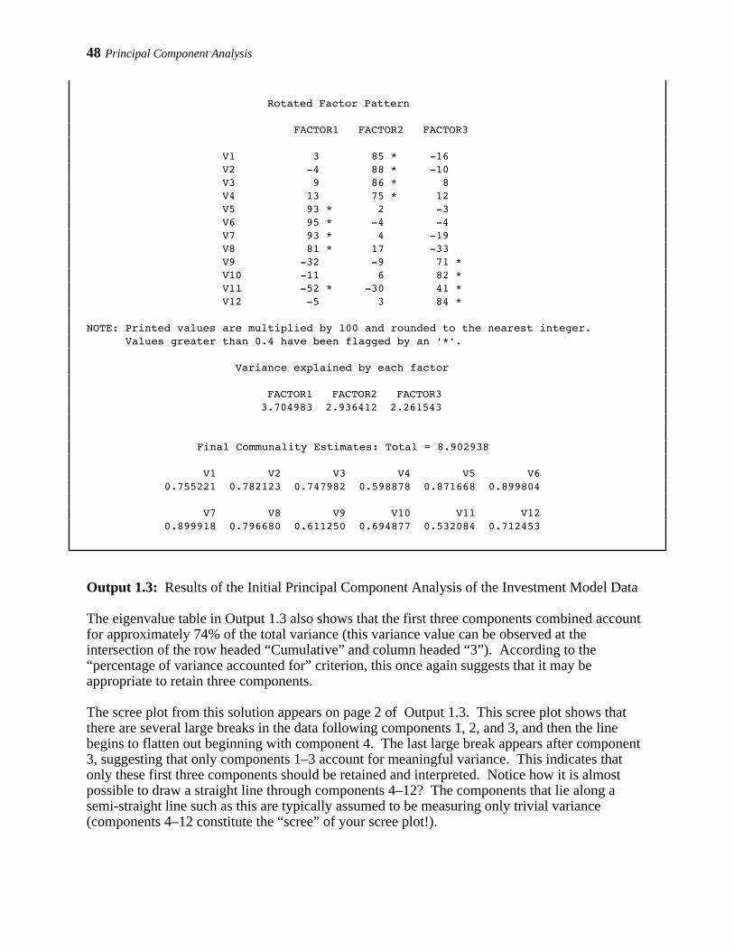
48 Principal Component Analysis
Rotated Factor Pattern
FACTOR1 FACTOR2 FACTOR3
V1 3 85 * -16 V2 -4 88 * -10 V3 9 86 * 8 V4 13 75 * 12 V5 93 * 2 -3 V6 95 * -4 -4 V7 93 * 4 -19 V8 81 * 17 -33 V9 -32 -9 71 * V10 -11 6 82 * V11 -52 * -30 41 * V12 -5 3 84 *
NOTE: Printed values are multiplied by 100 and rounded to the nearest integer. Values greater than 0.4 have been flagged by an '*'.
Variance explained by each factor
FACTOR1 FACTOR2 FACTOR3 3.704983 2.936412 2.261543
Final Communality Estimates: Total = 8.902938
V1 V2 V3 V4 V5 V6 0.755221 0.782123 0.747982 0.598878 0.871668 0.899804
V7 V8 V9 V10 V11 V12 0.899918 0.796680 0.611250 0.694877 0.532084 0.712453
Output 1.3: Results of the Initial Principal Component Analysis of the Investment Model Data
The eigenvalue table in Output 1.3 also shows that the first three components combined accountfor approximately 74% of the total variance (this variance value can be observed at theintersection of the row headed “Cumulative” and column headed “3”). According to the“percentage of variance accounted for” criterion, this once again suggests that it may beappropriate to retain three components.
The scree plot from this solution appears on page 2 of Output 1.3. This scree plot shows thatthere are several large breaks in the data following components 1, 2, and 3, and then the linebegins to flatten out beginning with component 4. The last large break appears after component3, suggesting that only components 1–3 account for meaningful variance. This indicates thatonly these first three components should be retained and interpreted. Notice how it is almostpossible to draw a straight line through components 4–12? The components that lie along asemi-straight line such as this are typically assumed to be measuring only trivial variance(components 4–12 constitute the “scree” of your scree plot!).

Principal Component Analysis 49
So far, the results from the eigenvalue-one criterion, the variance accounted for criterion, and thescree plot have converged in suggesting that a three-component solution may be appropriate. Itis now time to review the rotated factor pattern to see if such a solution is interpretable. Thismatrix is presented on page 4 of Output 1.3.
Following the guidelines provided earlier, you begin your interpretation by looking forfactorially complex items; that is, items with meaningful loadings for more than one component. A review shows that item 11 (variable V11) is a complex item, loading on both components 1and 3. Item 11 is therefore scratched out. Except for this item, the solution is otherwise fairlyclean.
To interpret component 1, you read down the column for FACTOR1 and see that items 5–8display significant loadings for this component (remember that item 11 has been scatched out). These items are:
_____ 5. I have invested a great deal of time in my current relationship.
_____ 6. I have invested a great deal of energy in my current relationship.
_____ 7. I have invested a lot of my personal resources (e.g., money) indeveloping my current relationship.
_____ 8. My partner and I have developed a lot of mutual friends which Imight lose if we were to break up.
All of these items deal with the investments that subjects have made in their relationships, so itmakes sense to label this the “investment size” component.
The rotated factor pattern shows that items 1–4 displayed meaningful loadings for component 2.These items are:
_____ 1. I am satisfied with my current relationship.
_____ 2. My current relationship comes close to my ideal relationship.
_____ 3. I am more satisfied with my relationship than is the averageperson.
_____ 4. I feel good about my current relationship.
Given the content of the preceding items, it seems reasonable to label component 2 the“satisfaction” component.
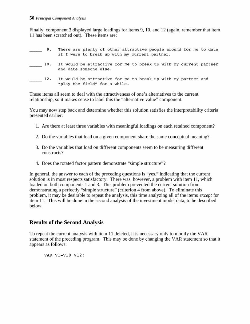
50 Principal Component Analysis
Finally, component 3 displayed large loadings for items 9, 10, and 12 (again, remember that item11 has been scratched out). These items are:
_____ 9. There are plenty of other attractive people around for me to dateif I were to break up with my current partner.
_____ 10. It would be attractive for me to break up with my current partnerand date someone else.
_____ 12. It would be attractive for me to break up with my partner and“play the field” for a while.
These items all seem to deal with the attractiveness of one’s alternatives to the currentrelationship, so it makes sense to label this the “alternative value” component.
You may now step back and determine whether this solution satisfies the interpretability criteriapresented earlier:
1. Are there at least three variables with meaningful loadings on each retained component?
2. Do the variables that load on a given component share the same conceptual meaning?
3. Do the variables that load on different components seem to be measuring differentconstructs?
4. Does the rotated factor pattern demonstrate “simple structure”?
In general, the answer to each of the preceding questions is “yes,” indicating that the currentsolution is in most respects satisfactory. There was, however, a problem with item 11, whichloaded on both components 1 and 3. This problem prevented the current solution fromdemonstrating a perfectly “simple structure” (criterion 4 from above). To eliminate thisproblem, it may be desirable to repeat the analysis, this time analyzing all of the items except foritem 11. This will be done in the second analysis of the investment model data, to be describedbelow.
Results of the Second Analysis
To repeat the current analysis with item 11 deleted, it is necessary only to modify the VARstatement of the preceding program. This may be done by changing the VAR statement so that itappears as follows:
VAR V1-V10 V12;

Principal Component Analysis 51
All other aspects of the program would remain as they were previously. The eigenvalue table,scree plot, the unrotated factor pattern, the rotated factor pattern, and final communalityestimates obtained from this revised program appear in Output 1.4:
The SAS System 1
Initial Factor Method: Principal Components
Prior Communality Estimates: ONE
Eigenvalues of the Correlation Matrix: Total = 11 Average = 1
1 2 3 4 Eigenvalue 4.0241 2.7270 1.6898 0.6838 Difference 1.2970 1.0372 1.0060 0.1274 Proportion 0.3658 0.2479 0.1536 0.0622 Cumulative 0.3658 0.6137 0.7674 0.8295
5 6 7 8 Eigenvalue 0.5564 0.3963 0.3074 0.2668 Difference 0.1601 0.0889 0.0406 0.0798 Proportion 0.0506 0.0360 0.0279 0.0243 Cumulative 0.8801 0.9161 0.9441 0.9683
9 10 11 Eigenvalue 0.1869 0.1131 0.0486 Difference 0.0739 0.0645 Proportion 0.0170 0.0103 0.0044 Cumulative 0.9853 0.9956 1.0000
3 factors will be retained by the MINEIGEN criterion.

52 Principal Component Analysis
Initial Factor Method: Principal Components 2 Scree Plot of Eigenvalues
| 4.0 + 1 | | | | | 3.5 + | | | | | 3.0 + | | | 2 | |E 2.5 +i |g |e |n |v |a 2.0 +l |u |e |s | 3 | 1.5 + | | | | | 1.0 + | | | | 4 | 5 0.5 + | 6 | 7 | 8 | 9 | 0 1 0.0 + ----+-----+-----+-----+-----+-----+-----+-----+-----+-----+-----+-----+--- 0 1 2 3 4 5 6 7 8 9 10 11 Number

Principal Component Analysis 53
The SAS System 3
Initial Factor Method: Principal Components
Factor Pattern
FACTOR1 FACTOR2 FACTOR3
V1 38 77 * -17 V2 30 83 * -15 V3 32 80 * 8 V4 29 70 * 15 V5 83 * -23 38 V6 83 * -30 38 V7 89 * -24 24 V8 88 * -12 7 V9 -56 * 13 47 * V10 -44 * 22 70 * V12 -40 18 74 *
NOTE: Printed values are multiplied by 100 and rounded to the nearest integer. Values greater than 0.4 have been flagged by an '*'.
Variance explained by each factor
FACTOR1 FACTOR2 FACTOR3 4.024086 2.727039 1.689791
Final Communality Estimates: Total = 8.440916
V1 V2 V3 V4 V5 V6 0.772386 0.798289 0.748233 0.591921 0.882544 0.921349
V7 V8 V9 V10 V12 0.904096 0.796623 0.553800 0.736193 0.735482
The SAS System 4
Rotation Method: Varimax
Orthogonal Transformation Matrix
1 2 3
1 0.84709 0.32928 -0.41715 2 -0.27787 0.94351 0.18051 3 0.45303 -0.03699 0.89073

54 Principal Component Analysis
Rotated Factor Pattern
FACTOR1 FACTOR2 FACTOR3
V1 3 86 * -17 V2 -4 89 * -11 V3 8 86 * 8 V4 12 75 * 14 V5 94 * 4 -4 V6 96 * -2 -6 V7 93 * 5 -20 V8 81 * 18 -33 V9 -30 -8 68 * V10 -12 4 85 * V12 -5 1 86 *
NOTE: Printed values are multiplied by 100 and rounded to the nearest integer. Values greater than 0.4 have been flagged by an '*'.
Variance explained by each factor
FACTOR1 FACTOR2 FACTOR3 3.444866 2.866255 2.129795
Final Communality Estimates: Total = 8.440916
V1 V2 V3 V4 V5 V6 0.772386 0.798289 0.748233 0.591921 0.882544 0.921349
V7 V8 V9 V10 V12 0.904096 0.796623 0.553800 0.736193 0.735482
Output 1.4: Results of the Second Analysis of the Investment Model Data
The results obtained when item 11 was dropped from the analysis are very similar to thoseobtained when it was included. The eigenvalue table of Output 1.4 shows that the eigenvalue-one criterion would again result in retaining three components. The first three componentsaccount for 77% of the total variance, which means that three components would also be retained if you used the variance-accounted-for criterion. Finally, the scree plot from page 2of Output 1.4 is just a bit cleaner than had been observed with the initial analysis: The breakbetween components 3 and 4 is now slightly more distinct, and the eigenvalues again level offafter this break. This means that three components would also likely be retained if the scree testwere used to solve the number-of-components problem.
The biggest change can be seen in the rotated factor pattern, which appears on page 4 of Output 1.4. The solution is now cleaner, in the sense that no item now loads on more thanone component. In this sense, the current results demonstrate a somewhat simpler structurethan had been demonstrated by the initial analysis of the investment model data.
Principal Component Analysis 55
Conclusion
Principal component analysis is a powerful tool for reducing a number of observed variables intoa smaller number of artificial variables that account for most of the variance in the data set. It isparticularly useful when you need a data reduction procedure that makes no assumptionsconcerning an underlying causal structure that is responsible for covariation in the data. When itis possible to postulate the existence of such an underlying causal structure, it may be moreappropriate to analyze the data using exploratory factor analysis.
Both principal component analysis and factor analysis are often used to construct multiple-itemscales from the items that constitute questionnaires. Regardless of which method is used, oncethese scales have been developed it is often desirable to assess their reliability by computingcoefficient alpha: an index of internal consistency reliability. Chapter 3 shows how this can bedone using the SAS System’s PROC CORR.
Appendix: Assumptions Underlying Principal Component Analysis
Because a principal component analysis is performed on a matrix of Pearson correlationcoefficients, the data should satisfy the assumptions for this statistic. These assumptions aredescribed in detail in Chapter 6, “Measures of Bivariate Association,” of Hatcher & Stepanski(1994) and are briefly reviewed here:
• Interval-level measurement . All analyzed variables should be assessed on an interval or ratiolevel of measurement.
• Random sampling . Each subject will contribute one score on each observed variable. Thesesets of scores should represent a random sample drawn from the population of interest.
• Linearity . The relationship between all observed variables should be linear.
• Normal distributions . Each observed variable should be normally distributed. Variables thatdemonstrate marked skewness or kurtosis may be transformed to better approximate normality(see Rummel, 1970).
• Bivariate normal distribution. Each pair of observed variables should display a bivariatenormal distribution; e.g., they should form an elliptical scattergram when plotted. However,the Pearson correlation coefficient is robust against violations of this assumption when thesample size is greater than 25.

56 Principal Component Analysis
References
Cattell, R. B. (1966). The scree test for the number of factors. Multivariate Behavioral Research, 1, 245-276.
Hatcher, L. & Stepanski, E. (1994). A step-by-step approach to using the SAS system for univariateand multivariate statistics . Cary, NC: SAS Institute Inc.
Kaiser, H. F. (1960). The application of electronic computers to factor analysis. Educational andPsychological Measurement, 20, 141-151.
Kim, J. O. & Mueller, C. W. (1978a). Introduction to factor analysis: What it is and how to do it. Beverly Hills, CA: Sage.
Kim, J. O. & Mueller, C. W. (1978b). Factor analysis: Statistical methods and practical issues. Beverly Hills, CA: Sage.
Rummel, R. J. (1970). Applied factor analysis. Evanston, IL: Northwestern University Press.
Rusbult, C.E. (1980). Commitment and satisfaction in romantic associations: A test of theinvestment model. Journal of Experimental Social Psychology, 16, 172-186.
SAS Institute Inc. (1989). SAS/STAT users guide, version 6, fourth edition, volume 1. Cary, NC: SAS Institute Inc.
Spector, P.E. (1992). Summated rating scale construction: An introduction. Newbury Park, CA: Sage.
Stevens, J. (1986). Applied multivariate statistics for the social sciences. Hillsdale, NJ: LawrenceErlbaum Associates.