principal component analysis and side-channel attacks
TRANSCRIPT

Principal Component Analysisand Side-Channel Attacks -
Master Thesis
Jip HogenboomDepartment of Computing Science
Digital SecurityRadboud University Nijmegen, The Netherlands
August, [email protected]
Thesis No. 634Supervisors:
Lejla Batina (Radboud University Nijmegen)Jasper van Woudenberg (Riscure B.V. Delft)


Abstract
Differential Power Analysis is commonly used to obtain information about the secretkey used in cryptographic devices. It requires power traces, which usually are high di-mensional, but may leak key information at multiple time instances. Power traces maybe misaligned, which reduces the effectiveness of DPA. Principal Component Analysis isa powerful tool which is used in different research areas to identify trends in a dataset.Principal Components are introduced which describe the relationships within the data.The largest principal components capture the data with the largest variance. ThesePrincipal Components can be used to reduce the noise in a dataset or to transform thedataset in terms of these components.We propose the use of Principal Component Analysis to improve the correlation for thecorrect key guess for Differential Power Analysis attacks on simulated DES traces, soft-ware DES traces, hardware DES traces and hardware AES-256 traces. Since PrincipalComponent Analysis does not consider the time domain, but instead finds the maximumvariance within a dataset, we still find the correct key in the presence of countermeasureslike introducing random delays. We introduce a new way of determining key candidatesby calculating the absolute average value of the correlation traces after a DPA attack ona PCA-transformed trace. A comparison between PCA and static alignment is made.We conclude that Principal Component Analysis can successfully be used as a prepro-cessing technique to reduce the noise in a traceset and improve the correlation for thecorrect key guess for Differential Power Analysis attacks.
i


Acknowledgements
First of all, I would like to thank Lejla Batina and Jasper van Woudenberg for theirtime, their guidance and their support. Especially during the final weeks, when theirfeedback was the most needed.My thanks go to Jing Pan, who gave valuable comments during the project.I would like to thank Marc Witteman from Riscure B.V. for providing me the opportu-nity to pursue this project. Also all colleagues at Riscure B.V. are thanked for makingthe trip to Delft worthwhile. Further I would like to thank Riscure B.V. as a whole forproviding the lunches and the facilities I needed for this project.I would specifically like to thank Yang Li and Kazuo Sakiyama of The University ofElectro-Communications in Tokyo, Japan who provided us with the SASEBO traces. Iwould not have been able to complete the SASEBO experiments without them.Further, I would like to thank Wojciech Mostowski for guiding me through the wholeprocess of writing a research paper, getting it accepted, and presenting it at WISSEC’09 which made writing this thesis and presenting it much easier.Thanks to the employee from the ARBO, who came to me in the second week of theproject and gave me some comments on my posture, I would not have come this farwithout him.
Finally I wish to thank my Father, my Mother and my Sister for always being therefor me and supporting me with whatever choice I make.
iii


Contents
Contents v
List of Figures ix
List of Tables xi
List of Abbreviations xiii
List of notations xv
1 Introduction 1
2 Data Encryption Standard (DES) 32.1 Introduction . . . . . . . . . . . . . . . . . . . . . . . . . . . . . . . . . . 32.2 DES . . . . . . . . . . . . . . . . . . . . . . . . . . . . . . . . . . . . . . 32.3 3-DES . . . . . . . . . . . . . . . . . . . . . . . . . . . . . . . . . . . . . 4
3 Side-Channel Attacks and Differential Power Analysis 73.1 Introduction . . . . . . . . . . . . . . . . . . . . . . . . . . . . . . . . . . 73.2 Power consumption . . . . . . . . . . . . . . . . . . . . . . . . . . . . . . 83.3 Simple Power Analysis (SPA) . . . . . . . . . . . . . . . . . . . . . . . . 93.4 Differential Power Analysis (DPA) . . . . . . . . . . . . . . . . . . . . . 103.5 Template attacks . . . . . . . . . . . . . . . . . . . . . . . . . . . . . . . 11
3.5.1 Number of traces . . . . . . . . . . . . . . . . . . . . . . . . . . . 113.6 Power model . . . . . . . . . . . . . . . . . . . . . . . . . . . . . . . . . 11
3.6.1 Hamming Distance model . . . . . . . . . . . . . . . . . . . . . . 123.6.2 Hamming Weight model . . . . . . . . . . . . . . . . . . . . . . . 123.6.3 Other models . . . . . . . . . . . . . . . . . . . . . . . . . . . . . 12
3.7 Side Channel Analysis distinguishers . . . . . . . . . . . . . . . . . . . . 123.7.1 Difference of means . . . . . . . . . . . . . . . . . . . . . . . . . . 133.7.2 Correlation . . . . . . . . . . . . . . . . . . . . . . . . . . . . . . 13
3.8 Common measurement setup . . . . . . . . . . . . . . . . . . . . . . . . 14
4 Countermeasures against Differential Power Analysis 174.1 Introduction . . . . . . . . . . . . . . . . . . . . . . . . . . . . . . . . . . 174.2 Hiding . . . . . . . . . . . . . . . . . . . . . . . . . . . . . . . . . . . . . 184.3 Masking . . . . . . . . . . . . . . . . . . . . . . . . . . . . . . . . . . . . 18
5 Principal Component Analysis (PCA) 215.1 Introduction . . . . . . . . . . . . . . . . . . . . . . . . . . . . . . . . . . 215.2 Mechanics . . . . . . . . . . . . . . . . . . . . . . . . . . . . . . . . . . . 225.3 Choosing the right number of principal components to keep . . . . . . . 23
5.3.1 Cumulative percentage of total variation . . . . . . . . . . . . . . 235.3.2 Scree test . . . . . . . . . . . . . . . . . . . . . . . . . . . . . . . 23
5.4 Applications for side-channel attacks . . . . . . . . . . . . . . . . . . . . 24
v

Contents
5.4.1 PCA transformation . . . . . . . . . . . . . . . . . . . . . . . . . 245.4.2 Noise reduction . . . . . . . . . . . . . . . . . . . . . . . . . . . . 24
6 Experiments 256.1 Introduction . . . . . . . . . . . . . . . . . . . . . . . . . . . . . . . . . . 256.2 Measurement setup . . . . . . . . . . . . . . . . . . . . . . . . . . . . . . 25
6.2.1 Hardware . . . . . . . . . . . . . . . . . . . . . . . . . . . . . . . 256.2.2 Software . . . . . . . . . . . . . . . . . . . . . . . . . . . . . . . . 26
6.3 Obtaining traces . . . . . . . . . . . . . . . . . . . . . . . . . . . . . . . 276.3.1 Smartcard . . . . . . . . . . . . . . . . . . . . . . . . . . . . . . . 276.3.2 SASEBO . . . . . . . . . . . . . . . . . . . . . . . . . . . . . . . 28
7 Principal Component Analysis and noise reduction - Experiments 297.1 Introduction . . . . . . . . . . . . . . . . . . . . . . . . . . . . . . . . . . 297.2 Simulated traceset (DES) . . . . . . . . . . . . . . . . . . . . . . . . . . 29
7.2.1 Experiments . . . . . . . . . . . . . . . . . . . . . . . . . . . . . 307.2.2 Discussion . . . . . . . . . . . . . . . . . . . . . . . . . . . . . . . 32
7.3 Real traceset (Software DES) . . . . . . . . . . . . . . . . . . . . . . . . 327.3.1 Experiments . . . . . . . . . . . . . . . . . . . . . . . . . . . . . 337.3.2 Discussion . . . . . . . . . . . . . . . . . . . . . . . . . . . . . . . 35
7.4 Real traceset (Hardware DES) . . . . . . . . . . . . . . . . . . . . . . . 357.4.1 Experiments . . . . . . . . . . . . . . . . . . . . . . . . . . . . . 357.4.2 Discussion . . . . . . . . . . . . . . . . . . . . . . . . . . . . . . . 36
7.5 SASEBO-R (AES-256) . . . . . . . . . . . . . . . . . . . . . . . . . . . . 367.5.1 Experiments . . . . . . . . . . . . . . . . . . . . . . . . . . . . . 377.5.2 Discussion . . . . . . . . . . . . . . . . . . . . . . . . . . . . . . . 37
7.6 How many and which components should be kept using power traces . . 377.6.1 Discussion . . . . . . . . . . . . . . . . . . . . . . . . . . . . . . . 38
8 Principal Component Analysis and transformation - Experiments 418.1 Introduction . . . . . . . . . . . . . . . . . . . . . . . . . . . . . . . . . . 418.2 Real traceset (Software DES) . . . . . . . . . . . . . . . . . . . . . . . . 41
8.2.1 Experiments . . . . . . . . . . . . . . . . . . . . . . . . . . . . . 428.2.2 Discussion . . . . . . . . . . . . . . . . . . . . . . . . . . . . . . . 43
8.3 Real traceset (Hardware DES) . . . . . . . . . . . . . . . . . . . . . . . 438.3.1 Experiments . . . . . . . . . . . . . . . . . . . . . . . . . . . . . 438.3.2 Discussion . . . . . . . . . . . . . . . . . . . . . . . . . . . . . . . 44
8.4 SASEBO-R (AES-256) . . . . . . . . . . . . . . . . . . . . . . . . . . . . 448.4.1 Experiments . . . . . . . . . . . . . . . . . . . . . . . . . . . . . 448.4.2 Discussion . . . . . . . . . . . . . . . . . . . . . . . . . . . . . . . 44
8.5 Simulated traceset (DES) . . . . . . . . . . . . . . . . . . . . . . . . . . 458.5.1 Experiments . . . . . . . . . . . . . . . . . . . . . . . . . . . . . 458.5.2 Discussion . . . . . . . . . . . . . . . . . . . . . . . . . . . . . . . 45
9 Alignment 479.1 Introduction . . . . . . . . . . . . . . . . . . . . . . . . . . . . . . . . . . 47
9.1.1 DPA on misaligned traces . . . . . . . . . . . . . . . . . . . . . . 489.1.2 Alignment before attack . . . . . . . . . . . . . . . . . . . . . . . 489.1.3 Preprocess power traces before attack . . . . . . . . . . . . . . . 49
9.2 PCA and Misalignment - Experiments . . . . . . . . . . . . . . . . . . . 499.2.1 Experiments . . . . . . . . . . . . . . . . . . . . . . . . . . . . . 499.2.2 A comparison between PCA and static alignment . . . . . . . . . 519.2.3 Random delays . . . . . . . . . . . . . . . . . . . . . . . . . . . . 519.2.4 Other algorithms . . . . . . . . . . . . . . . . . . . . . . . . . . . 539.2.5 Discussion . . . . . . . . . . . . . . . . . . . . . . . . . . . . . . . 53
vi

Contents
10 Conclusion 5510.1 Conclusion . . . . . . . . . . . . . . . . . . . . . . . . . . . . . . . . . . 5610.2 Further research . . . . . . . . . . . . . . . . . . . . . . . . . . . . . . . 57
Bibliography 59
Appendices 63Appendix A. PCAFilter source code . . . . . . . . . . . . . . . . . . . . . . . 65
vii

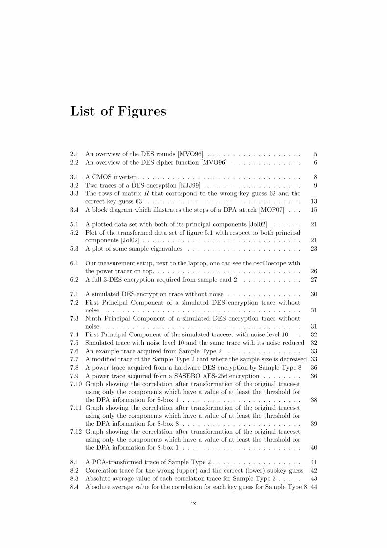
List of Figures
2.1 An overview of the DES rounds [MVO96] . . . . . . . . . . . . . . . . . . . 5
2.2 An overview of the DES cipher function [MVO96] . . . . . . . . . . . . . . 6
3.1 A CMOS inverter . . . . . . . . . . . . . . . . . . . . . . . . . . . . . . . . . 8
3.2 Two traces of a DES encryption [KJJ99] . . . . . . . . . . . . . . . . . . . . 9
3.3 The rows of matrix R that correspond to the wrong key guess 62 and thecorrect key guess 63 . . . . . . . . . . . . . . . . . . . . . . . . . . . . . . . 13
3.4 A block diagram which illustrates the steps of a DPA attack [MOP07] . . . 15
5.1 A plotted data set with both of its principal components [Jol02] . . . . . . 21
5.2 Plot of the transformed data set of figure 5.1 with respect to both principalcomponents [Jol02] . . . . . . . . . . . . . . . . . . . . . . . . . . . . . . . . 21
5.3 A plot of some sample eigenvalues . . . . . . . . . . . . . . . . . . . . . . . 23
6.1 Our measurement setup, next to the laptop, one can see the oscilloscope withthe power tracer on top. . . . . . . . . . . . . . . . . . . . . . . . . . . . . . 26
6.2 A full 3-DES encryption acquired from sample card 2 . . . . . . . . . . . . 27
7.1 A simulated DES encryption trace without noise . . . . . . . . . . . . . . . 30
7.2 First Principal Component of a simulated DES encryption trace withoutnoise . . . . . . . . . . . . . . . . . . . . . . . . . . . . . . . . . . . . . . . 31
7.3 Ninth Principal Component of a simulated DES encryption trace withoutnoise . . . . . . . . . . . . . . . . . . . . . . . . . . . . . . . . . . . . . . . 31
7.4 First Principal Component of the simulated traceset with noise level 10 . . 32
7.5 Simulated trace with noise level 10 and the same trace with its noise reduced 32
7.6 An example trace acquired from Sample Type 2 . . . . . . . . . . . . . . . 33
7.7 A modified trace of the Sample Type 2 card where the sample size is decreased 33
7.8 A power trace acquired from a hardware DES encryption by Sample Type 8 36
7.9 A power trace acquired from a SASEBO AES-256 encryption . . . . . . . . 36
7.10 Graph showing the correlation after transformation of the original tracesetusing only the components which have a value of at least the threshold forthe DPA information for S-box 1 . . . . . . . . . . . . . . . . . . . . . . . . 38
7.11 Graph showing the correlation after transformation of the original tracesetusing only the components which have a value of at least the threshold forthe DPA information for S-box 8 . . . . . . . . . . . . . . . . . . . . . . . . 39
7.12 Graph showing the correlation after transformation of the original tracesetusing only the components which have a value of at least the threshold forthe DPA information for S-box 1 . . . . . . . . . . . . . . . . . . . . . . . . 40
8.1 A PCA-transformed trace of Sample Type 2 . . . . . . . . . . . . . . . . . . 41
8.2 Correlation trace for the wrong (upper) and the correct (lower) subkey guess 42
8.3 Absolute average value of each correlation trace for Sample Type 2 . . . . . 43
8.4 Absolute average value for the correlation for each key guess for Sample Type 8 44
ix

List of Figures
8.5 Absolute average value for the correlation for each key byte for SASEBOAES-256 measurements . . . . . . . . . . . . . . . . . . . . . . . . . . . . . 45
8.6 Absolute average value for the correlation for each key guess for the simulatedtraces without noise . . . . . . . . . . . . . . . . . . . . . . . . . . . . . . . 45
9.1 Two misaligned traces . . . . . . . . . . . . . . . . . . . . . . . . . . . . . . 479.2 The two traces from figure 9.1 after an alignment step . . . . . . . . . . . . 489.3 Correlation trace for a wrong key guess (62) and for the correct key guess(63) 509.4 Absolute average value of each correlation trace . . . . . . . . . . . . . . . . 509.5 Selected components in the upper graph are used for analysis, the lower graph
shows the absolute average value of each correlation trace for those components 509.6 Transformed traceset from Sample Type 2 with random delays . . . . . . . 529.7 The 40th and the 41 principal component of a PCA transformed traceset
with random delays . . . . . . . . . . . . . . . . . . . . . . . . . . . . . . . 529.8 Absolute average value of the correlation graphs for the key guesses using
the transformed traceset . . . . . . . . . . . . . . . . . . . . . . . . . . . . . 53
x

List of Tables
9.1 Comparison between Static alignment and PCA . . . . . . . . . . . . . . . 51
xi


List of Abbreviations
AES Advanced Encryption StandardCMOS Complementary Metal Oxide SemiconductorCPA Correlation Power AnalysisDES Data Encryption StandardDPA Differential Power AnalysisDTL Dual-rail Transition LogicDTW Dynamic Time WarpingEA Elastic AlignmentECC Elliptic Curve CryptographyEEPROM Electrically Erasable Programmable Read-Only MemoryEMA ElectroMagnetic AnalysisFFT Fast Fourier TransformationFPGA Field-Programmable Gate ArrayHD Hamming DistanceHW Hamming WeightIP Initial PermutationMDPL Masked Dual-rail Precharge LogicMHz MegahertzPC Principal ComponentPCA Principal Component AnalysisRSL Random Switching LogicRFID Radio Frequency IDentificationRSA Rivest-Shamir-AdelmanSABL Sense Amplifier Based LogicSASEBO Side-channel Attack Standard Evaluation BoardSCA Side-Channel AnalysisSNR Signal-to-Noise RatioSPA Simple Power AnalysisWDDL Wave Dynamic Differential LogicXOR Exclusive-OR
xiii


List of notations
Σ Covariance matrixΛ Eigenvalue matrixck Index of the correct key in kct Index of the position in the power traces that leaks information in a DPA attackCov(X,Y ) Covariance of X and Yd Vector of calculated input/output valuesD Number of power traces used for a DPA attackDimx The xth dimension in a power traceH Matrix of hypothetical power consumption valuesi Indexk Subkey out of keyspace KK KeyspaceM Mean vectorn Number of samples in a power traceρ Correlation coefficientR Matrix which contains the results of a DPA attackT Matrix of power consumption valuesT Number of samples in a power tracet Power traceU Eigenvector matrix/PCA feature vectorV Matrix of hypothetical power consumption valuesV ar(X) Variance of XX Original dataset
X PCA transformed datasetZ Final matrix
xv


Chapter 1
Introduction
Side-channel attacks are indirect methods which are used to find secret keys in crypto-graphic devices. These devices include smartcards, set-top boxes and mobile phones. Onthese devices, cryptographic algorithms are implemented to ensure encrypted communi-cation. Smartcards can sometimes contain a software implementation of some algorithmbut they might also have a cryptographic co-processor, where the larger devices usu-ally have a dedicated hardware implementation. In this thesis, the Data EncryptionStandard (DES) and the Advanced Encryption Standard (AES) algorithms are used astarget encryption algorithms. The secret keys used for the algorithms are usually wellprotected within cryptographic devices. If the key of a device is found, the device isconsidered broken. Depending on the scenario where the device is used, an adversarycan cause serious harm. If, for example, the cryptographic key of a smartcard which isused in a Pay-TV application can be found, one can watch the channels for free. If thishappens at a large scale, this might have serious economic consequences. A widely usedmethod to recover secret keys is by making use of a side-channel.
Side-channel attacks make use of side-channel information, which is information thatcan be acquired from a cryptographic device that is not the plaintext nor the ciphertext.This information is leaked because of weaknesses in the physical implementation of thealgorithm.
An example of a widely used side-channel attack is Differential Power Analysis (DPA)[KJJ99]. The power consumption of a cryptographic device is dependent on the datawhich is being processed. The secret key is used during an encryption or a decryption.This means that the power consumption of a cryptographic device is dependent on theused key. This power consumption can be measured by creating power traces. DPAanalyses the statistics of the power measurements on a device in order to derive theused cryptographic key. Depending on the amount of noise in the measurements, a lotof power traces might be required in order for a DPA attack to be successful. Manu-facturers of cryptographic devices usually implement countermeasures on their devices.These countermeasures also complicate DPA substantially.
Principal Component Analysis (PCA) [Jol02] is a technique which is used to identifytrends in multidimensional datasets. It can be used to reduce the noise in a dataset ortransform the data in terms of lines that describe the relationships within the data thebest. It captures data with the same amount of variance in different, so-called, PrincipalComponents. The key leakage in power traces usually has a large amount of variance.Power measurements usually also contain noise. PCA can be used to reduce the amountof noise while keeping only the components which capture the key leakage.DPA uses the measurement data to find the used secret key. Since these measurementsusually contain a lot of noise, we could potentially obtain better results if we couldreduce this noise in some way.
1
1. Introduction
In this thesis, the effects of PCA on DPA attacks are analysed.
In order to perform a successful DPA attack, one needs to be sure that the sameoperation of the algorithm is executed at the same time within each power trace in orderto compare the values. This is called alignment. Power traces are easily misaligned sinceit is very hard to time the recording of a trace. Furthermore, there are countermeasuresagainst side-channel attack which introduce random time delays in the execution of thealgorithm which causes power traces to be even more misaligned. Different methodshave been proposed to make aligning traces easier, e.g. static alignment [MOP07] andelastic alignment [vWWB]. In this thesis, the effect of Principal Component Analysison misaligned traces is analysed. Also, a comparison is made between PCA and staticalignment in terms of their effect and the computation time.
We analyse power measurements which are taken from simulated DES encryptions,software DES (smartcard), hardware DES (smartcard) and hardware AES-256 (SASEBO-R).
Template attacks using Principal Component Attacks are described in [APSQ06].Before they perform a normal template attack, they transform the traces in order to beable to select relevant features. They use PCA to find the maximum variance. In thisthesis, we won’t touch the subject of template attacks. We make use of the same PCAtransformation, but dive more into noise reduction and look at the behaviour of PCAin the presence of countermeasures.
[BNSQ03] also touches upon Principal Component Analysis as a method to improvepower attacks. They cover the effect of PCA on Simple Power Analysis, while we studythe effect of PCA on Differential Power Analysis.
This thesis is organized as follows. Chapter 2 describes the DES algorithm sincethis is the algorithm which we use the most for our experiments. Chapter 3 describeswhat side-channel attacks are. Since our focus is on power analysis, we discuss SimplePower Analysis and Differential Power Analysis in particular. Countermeasures againstDPA are covered in Chapter 4 since we want to analyse the effect PCA has in the pres-ence of one of these countermeasures. Chapter 5 describes the background of PrincipalComponent Analysis. Our measurement setup and the way we acquire traces can befound in Chapter 6. Our experiments with PCA and noise reduction on the differenttracesets are described in Chapter 7. Chapter 8 contains the experiments with a PCAtransformation of power measurements. The alignment problem and the effect of PCAon this problem is discussed in Chapter 9. In Chapter 10 our conclusion and furtherresearch is described.
2

Chapter 2
Data Encryption Standard (DES)
2.1 Introduction
The Data Encryption Standard (DES) is a block cipher which was invented in 1970by IBM. In 1976 it became a Federal Information Processing Standard (FIPS) in theUnited States. After its initial publication, the standard has been revised 3 times. DEScan not be considered secure anymore, [Wie94] shows how to build an exhaustive DESkey search machine for 1 million dollar that can find a key in 3.5 hours on average. Thisis the reason why the use of Triple-DES is advised [US 99]. Triple-DES is very widelyused in practice since it still is considered to be secure.Since the Advanced Encryption Standard (AES) became the successor of Triple-DES,US government agencies have until 2030 to switch to AES. After 2030, they are notallowed to use Triple-DES anymore [Bar08].
For our experiments we mostly target DES since we have access to a DES simulator,a software DES implementation and a hardware DES implementation.
2.2 DES
DES makes use of a 64-bit key, of which only 56 bits are actually used by the algorithm.The other 8 bits are only used for error-detection.
The DES algorithm consists of 15 identical rounds. The 16th round uses the samefunctions as the other 15, but does not swap the L and R block afterwards (irregularswap). For an overview, see figure 2.1. DES takes blocks of 64 bits of plaintext asinput and returns an output of blocks of 64 bits of ciphertext. The first operation inthe algorithm is a permutation of the plaintext. This permutation is called the InitialPermutation (IP ). In this step, the bits of the plaintext are switched in a fixed order.Then the 64-bit block is split into two 32-bit blocks, a left (L) and a right (R) halve (L0
and R0 in figure 2.1).
After these initial steps, the round operations start. During each round, a 48 bitblock (Kn) of the key is derived by permuting a, depending on the round number (n),selection of bits from the full key. Then the previous L and R block are used to derivethe next block using a cipher function (f) (2.1).
Ln = Rn−1
Rn = Ln−1 ⊕ f(Rn−1,Kn) (2.1)
The cipher function f takes the 32-bit block R, and expands it using an expansionfunction E to a block of 48 bits. This expansion function is a fixed permutation wherethe bits in some positions are copied to other positions in order to make a 48-bit block.
3

2. Data Encryption Standard (DES)
This result is then added bit-by-bit to the 48 bit key (modulo 2). This result is thendivided into 8 blocks of 6 bits (2.2). The function further contains 8 substitution boxes(S1,...,S8) which are commonly called S-boxes. These boxes take a 6-bit input, andresult in a 4-bit output in order to get a result of 8 x 4 = 32 bits again. The S-boxes area lookup table where, depending on the input, the corresponding output can be found.The principle is the same for all S-boxes but they use different tables. They are used toreduce the relationship between the key and the ciphertext.
The final operation within this function f is a permutation operation which switchesthe bits to obtain the final result (2.3).
B1, B2, ..., B8 = K ⊕ E(R) (2.2)f(R,K) = P (S1(B1), S2(B2), ..., S8(B8)) (2.3)
For an overview of the cipher function f , see figure 2.2.
The final operation is a Final Permutation (FP) which switches the bits of the ci-phertext in a fixed order. This operation is the inverse of the initial permutation tofacilitate easy decryption.
Decryption works by running the algorithm with inverted rounds and by makingsure that the right keys are used in subsequent rounds.
Modern equipment (e.g. the Cost-Optimized PArallel COde Breaker (COPACOBANA)1)can relatively easy brute-force the 56-bit key which is used by DES. Also, DES is proneto a Linear [Mat94] and Differential Cryptanalysis attack [BS93]. Because of these is-sues, there became a need for a new, more secure, algorithm. 3-DES was proposed[US 99].
2.3 3-DES
Triple DES (also 3-DES or Triple Data Encryption Algorithm (TDEA)) basically con-sists of a DES encryption using one key, followed by a DES decryption using anotherkey. The resulting ciphertext is encrypted again (2.1).
ciphertext = Ek3(E−1k2 (Ek1(plaintext))) (2.3)
The standard defines three ways how this key bundle (k1, k2, k3) can be chosen:
• k1, k2 and k3 are independent keys (168 bit key).
• k1 and k2 are independent keys and k1 = k3 (112 bit key).
• k1 = k2 = k3. This is basically the same as a single DES encryption since thedecryption cancels out the first encryption (56 bit key). Using this key bundlemakes the algorithm backwards compatible with DES.
For more information on DES or Triple-DES, the reader is referred to [US 99].
1http://www.copacobana.org
4

2.3. 3-DES
Figure 2.1: An overview of the DES rounds [MVO96]
5

2. Data Encryption Standard (DES)
Figure 2.2: An overview of the DES cipher function [MVO96]
6
Chapter 3
Side-Channel Attacks andDifferential Power Analysis
3.1 Introduction
Cryptographic devices like smartcards, set-top boxes, mobile phones, PDA’s and RFIDtags are becoming a large part of modern society. Their private keys, which are usedfor the cryptographic algorithms are usually kept safe in a secure way. Side-channelattacks use weaknesses in the physical implementation of an algorithm in order to findexploitable information other than the plaintext or ciphertext. Testing laboratories useside-channel attacks to test the protection of a cryptographic device. Researchers applyside-channel attacks to test new countermeasures or try to invent new attacks. Finallythere are the ’bad guys’ who actually use side-channel attacks to find the secret keywithin a cryptographic device in order to break it.
The main advantage of side-channel attacks is that they are applicable to mostpresent circuit technologies. In most cryptographic devices, a secure cryptographicalgorithm is used, where secure means that performing a brute force attack on the al-gorithm to find the secret key is infeasible. The main property which is exploited byside-channel attacks, is that the physical implementation of these algorithms can leaksome amount of information.
If some information about the algorithm is known (either by general knowledgeor reverse engineering), it might be possible to measure some characteristics of thesystem in order to exploit this information. There are two categories of side-channelattacks, passive and active attacks. Examples of passive side-channels that may beused are power [KJJ99], electromagnetic radiation [QS01], timing [Koc96] and sound[ST04],[Bri91]. Active side-channel attacks are e.g. fault injection [BDL97] and cold-boot attacks [HSH+09].
For many secure applications, side-channel testing is mandatory. There are multipletesting laboratories who can evaluate these cryptographic devices, Riscure B.V. is one ofthem. There are different frameworks which describe how a cryptographic device shouldbe protected. If the device is considered safe according to these frameworks, they canbe certified. An example of such a framework is the Common Criteria for InformationTechnology Security Evaluation (Common Criteria or CC).
The subject of this thesis are power analysis attacks. There are two basic typesof attacks, Simple Power Analysis (SPA) and Differential Power Analysis (DPA). Thereason they work and their main differences will be discussed in the following sections.It is important to note that power analysis attacks are usually non-invasive, which
7
3. Side-Channel Attacks and Differential Power Analysis
means that mounting an attack does not cause damage to the device and thus might beunnoticed.
3.2 Power consumption
The power consumption of a cryptographic device can leak information about the secretkey used within the device since it is dependent on the data that the circuit processes.This is caused by the low-level design of these devices. The basis of almost every elec-tronic device are CMOS (Complementary Metal Oxide Semiconductor) circuits. Thistechnology has a characteristic power consumption which can be used in power analysisattacks. A CMOS circuit consists of logic cells which contribute to the total powerusage of the circuit. The power consumption depends on the number of logic cells, theconnections between them and how the cells are built. A CMOS circuit is provided witha constant supply voltage Vdd.
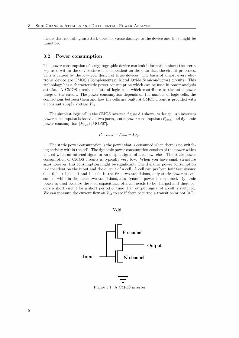
The simplest logic cell is the CMOS inverter, figure 3.1 shows its design. An inverterspower consumption is based on two parts, static power consumption (Pstat) and dynamicpower consumption (Pdyn) [MOP07].
Pinverter = Pstat + Pdyn
The static power consumption is the power that is consumed when there is no switch-ing activity within the cell. The dynamic power consumption consists of the power whichis used when an internal signal or an output signal of a cell switches. The static powerconsumption of CMOS circuits is typically very low. When you have small structuresizes however, this consumption might be significant. The dynamic power consumptionis dependent on the input and the output of a cell. A cell can perform four transitions:0 → 0, 1 → 1, 0 → 1 and 1 → 0. In the first two transitions, only static power is con-sumed, while in the latter two transitions, also dynamic power is consumed. Dynamicpower is used because the load capacitance of a cell needs to be charged and there oc-curs a short circuit for a short period of time if an output signal of a cell is switched.We can measure the current flow on Vdd to see if there occurred a transition or not [AO].
Figure 3.1: A CMOS inverter
8

3.3. Simple Power Analysis (SPA)
3.3 Simple Power Analysis (SPA)
Simple Power Analysis (SPA) was, together with Differential Power Analysis (DPA),first introduced in 1999 by Paul Kocher et al. [KJJ99]. Even though the name suggestsotherwise, SPA is not that simple.
In order to mount an SPA attack, only one or several power traces of a cryptographicdevice executing the encryption or decryption of a known input are needed. A prereq-uisite for this attack is some knowledge of the implementation of the algorithm. Ideally,these power traces only show the power consumption of the gates used in the encryp-tion/decryption. This is however not the case, there always exists some amount of noise.
The total power consumption at some point in time consists of the constant powerconsumption and the electronic noise, the switching noise and an exploitable part (3.1)[MOP07].
Ptotal = Pconstant + Pswitchingnoise + Pelectricnoise + Pexp (3.1)
The more measurements one has, the easier it is to reduce the noise by taking themean of the traces. SPA attacks work for example on algorithms which have condi-tional branches. This means that they execute different instructions depending on theprocessed value. If one has have knowledge of the implementation of the algorithm,one might be able to find which branch was taken, and what the value of a specific bitmust have been. The DES algorithm contains a lot of permutations. Software imple-mentations of this algorithm might use a lot of conditional branches [KJJ99]. Withoutcountermeasures, these branches can easily be found in power traces when performingSPA. Figure 3.2 shows two traces of a DES encryption, the difference is in clock cycle6 where in the upper trace the microprocessor performs a jump instruction which isnot present in the lower trace [KJJ99]. Using this method it might be possible to finddifferent bit values and reconstruct parts of the used key.
Figure 3.2: Two traces of a DES encryption [KJJ99]
According to Kocher et al. [KJJ99], it is fairly easy to prevent SPA attacks by notusing conditional branches in software implementations. Also, most hardware imple-mentations have very small power consumption variations which means that a single
9
3. Side-Channel Attacks and Differential Power Analysis
trace might not be enough to find the differences. In order to make power analysis moresuccessful, Differential Power Analysis was proposed.
3.4 Differential Power Analysis (DPA)
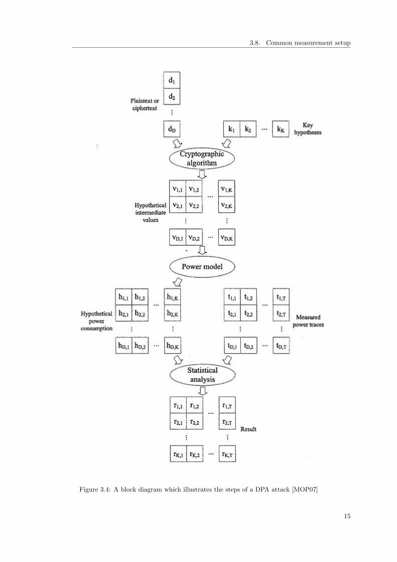
Differential Power Analysis is an advanced power analysis technique which uses sta-tistical methods in order to define a relationship between power measurements and apredicted power consumption of the device. This power consumption can be predictedby different methods which will be explained below. In order to mount a DPA attack, nodetailed knowledge of the implementation of the cryptographic algorithm on the deviceis needed. Since this usually is the case when attacking a device, this method is verysuitable. The main drawback is that DPA usually needs a lot of traces in order to findthe relation. Acquiring the necessary amount of traces might take a long time, or mightnot be possible at all due to different countermeasures which, for example, only allowthe device to perform a limited number of encryptions in a fixed amount of time. Theinfluence of the processed data on the power is analysed at a fixed moment in time.DPA attacks are typically done in 5 steps [MOP07], see figure 3.4 for an overview.
• First an intermediate result of the cryptographic algorithm is chosen where a non-constant data value d is known. The value is usually the plaintext when attackingthe first round and the ciphertext when attacking the final round. The functionfor this intermediate result is f(d, k) where k is a small part of the key.
• Then we take power measurements of encryption or decryption operations of thedevice.We choose a sufficiently large number D of plaintexts. Depending on the chosenposition in the algorithm in the first step, we can calculate beforehand what thevalue of d should be for each encryption/decryption run D. We define a vectord = (d1, ..., dD).For each of these D runs, a power trace is created with T samples. Hence we cancreate a matrix T of size D ∗ T which contains the power traces corresponding toeach data block.
• The third step is to calculate the hypothetical values of d for every possible subkeyk out of the key space K. In the case of DES, this key space has size 64 since thereare 64 different subkeys for each S-box. We choose a position to attack where theused subkey is small. Since the subkey of an S-box is typically small enough todo an exhaustive search, we can calculate the function f(d, k) for each data valued and each subkey k. These results can be stored in a matrix V of size D ∗ K.One of the keys we have tried here must correspond to the actual subkey used inthe device. The goal is to find the column in this matrix V which was processedduring the encryption/decryption runs.
• The fourth step is to map the hypothetical intermediate values to hypotheticalpower consumption values using a power model. This way we can simulate thepower consumption the processed data is expected to have. This power model willbe explained later. These calculations result in a matrix H of size D ∗K whichcontains these hypothetical power consumption values.
• The last step in a DPA attack is comparing the hypothetical power consumptionvalues to the measured power consumption values. The hypothetical power con-sumption values of each key hypothesis are compared with the power traces ateach position. This results in a matrix R of size K ∗ T which contains the resultsof the comparison. Depending on the used power model, there exists a relationbetween the hypothetical power consumption and the real power consumption. Wecan use statistical methods to derive this relation. If there are sufficient traces,
10
3.5. Template attacks
a suitable power model, and a suitable statistical analysis algorithm is used, thehighest value in this matrix will correspond to the correct key guess.
By repeating these steps for each S-box within the algorithm, one can derive allsubkeys.
The power traces must be perfectly aligned in order to be sure that the measuredvalues at the same moment in time are caused by the same operation within the algo-rithm. This alignment problem is explained in section 9.1.
3.5 Template attacks
The strongest kind of DPA attacks are template-based DPA attacks [AR03]. For atemplate attack, one needs full access to and control over a training device. This deviceis used to characterize the target device. Then a template is built for every possible keyusing the training device, the signal and the noise needs to be modelled. A capturedtrace of the target device is classified using these templates, the goal is to find thetemplate which fits best to the captured trace.
3.5.1 Number of traces
It is hard to estimate beforehand how many traces we need to acquire. On poorlyprotected devices this may be tens, but on well-protected hardware devices this may bemillions. In case of using the correlation coefficient, one needs to find out how manytraces are necessary in order to find which column of H has the strongest correlation toa column of T. [MOP07] provides a rule which is based on three assumptions:
• A DPA attack is successful if there is a significant peak in the row of the correctkey ck in the result matrix R.
• The power model fits the power consumption of the attacked device.
• The number of traces that are needed to see a peak only depends on the correlationbetween the correct key ck and the correct moment of time ct. The attackedintermediate result is processed in only a small number of samples as compared tothe whole power trace which means that many operations are executed that areindependent of this intermediate result. This means that most of the correlationsbetween ck and ct are zero. One needs to find if the correlation coefficient betweenck and ct is zero or not.
When we want to assess the number of traces which are needed for a DPA attackwith a confidence of 0.0001, the following formula can be used [MOP07]:
n = 3 + 8 3.719
ln2(1+ρck,ct1−ρck,ct
)
3.6 Power model
A DPA attack is most successful if the modelled power consumption is as close to thereal power consumption as possible. A basic netlist describes the cells of a circuit andthe connections between them. It could also include signal delays and rise and fall timesfor the signals in the circuit [MOP07]. If one has such a netlist, one can simulate thetransitions within the circuit. Then one can map the simulated transitions to a powertrace using a power model. The more precise the netlist is, the easier it is to createa correct power model. A generic model which can be used is the Hamming Distance(HD) model.
11
3. Side-Channel Attacks and Differential Power Analysis
3.6.1 Hamming Distance model
Since the power consumption strongly depends on the number of flips done by the tran-sistors within the circuit, it is possible to check how many of these had to be appliedto get from a value to another value. Depending on the device which is being attacked,and the knowledge of an attacker, he can usually make some assumptions about the waythe device is built.The Hamming Weight (HW) of a byte is the number of bits which are set to one in thebinary value. The Hamming Distance (HD) between two values is the number of zeroto one and one to zero transitions which have to occur in order to transform the firstvalue into the second value. This method uses a couple of assumptions while consideringCMOS. For example, it is assumed that zero to one and one to zero transitions havethe same power consumption. This is also assumed for zero to zero and one to onetransitions. Also, it is assumed that all cells contribute equally to the power consump-tion. Since this is a fairly easy power model which can be used to calculate the roughestimate of the power consumption relatively quickly, it is commonly used [MOP07]. Ifan attacker knows which values are being processed by a part of the netlist, he can usethe Hamming Distance model to simulate the power consumption.
3.6.2 Hamming Weight model
If an attacker does not know consecutive data values or has no knowledge of the netlist,the Hamming Weight model can be used. An attacker needs to know one value whichis processed. He assumes that the power consumption is proportional to the HammingWeight of the value. In CMOS circuits, the power consumption depends on the transi-tions and not on the processed values [MOP07].
For this model, we assume that before processing the known value v1, another, un-known value v0 is processed. There are multiple scenarios which can occur, dependingon the value of v0. If the bits of v0 are equal and constant, one gets that the simulatedpower consumption is directly or inversely proportional to the actual power consump-tion since if all bits of v0 are 0: HD(v0, v1) = HW (v0 ⊕ v1) = HW (v1). If all n bits ofv1 are 1: HD(v0, v1) = HW (v0 ⊕ v1) = n−HW (v1). This means that in this case theHW and the HD model have equivalent results.
There are other scenarios which are more likely to occur, for an explanation ofthese scenarios the interested reader is referred to section 3.3.2 of [MOP07]. The mainconclusion is that the HW model can be used instead of the HD model but it performsmuch worse since the relation between the Hamming Weight of v1 and the actual powerconsumption can become very weak.
3.6.3 Other models
If the power consumption of a specific device is known in more detail, a power model canbe created for that device in order to model the power consumption more effectively, andthus make a DPA attack more effective. There are various methods which can be usedto derive such a model, two examples are toggle counts [TV05] and SPICE simulation[Nag75].
3.7 Side Channel Analysis distinguishers
A side-channel analysis distinguisher is a statistical test which is used to determinethe relationship between the hypothetical power consumption and the measured powertraces. The difference of means and correlation are two of those distinguishers.
12

3.7. Side Channel Analysis distinguishers
3.7.1 Difference of means
The original, and first published, DPA attack makes use of the ”difference of means”method [KJJ99]. This method is used to determine the relationship between the hy-pothetical power consumption (matrix H mentioned above) and the measured powerconsumption (matrix T mentioned above). In step 4 only a binary power model can beused which means that hi,j can only be one or zero. This means that the power con-sumption can not be described with a high accuracy. The power consumption in eachcolumn of H is a function of the input data and the key hypothesis. If the key guess isincorrect, the value of hi will be correct with a probability of 1
2 for each plaintext. Anattacker can split the matrix T in two rows, one where hi is zero and one where hi isone. Then one can calculate the mean of both rows and subtract those from each other.The result with the largest peak, which indicates a big difference between the two rows,is the correct key since this indicates a relation between hck and some columns of T.
3.7.2 Correlation
Compared to the difference of means method, using the correlation uses more resources,but it is less sensitive to noise which means that it produces better results in most cases.Analysis using the correlation coefficient is also called Correlation Power Analysis (CPA)[BCO04]. The correlation coefficient ρ(X,Y ) defines the linear relationship between twopoints (X and Y ) of a trace and it can take values between plus and minus 1. Thecorrelation is defined as:
ρ(X,Y ) = Cov(X,Y )√V ar(X)·V ar(Y )
The correlation coefficient is used to determine the linear relationship between thehypothetical power consumption (H) and the measured power consumption (T ). Asshown before, in step 5 of a DPA attack, these estimated correlation coefficients arestored in the matrix R. This correlation coefficient can be calculated as:
ri,j =
∑D
d=1(Hd,i−Hi)·(Td,j−tj)√∑D
d=1(Hd,i−Hi)2·
∑D
d=1(Td,j−Tj)2
Figure 3.3: The rows of matrix R that correspond to the wrong key guess 62 and thecorrect key guess 63
Figure 3.3 shows two plotted rows of R, one for the wrong key guess (62) and onefor the correct key guess (63). The peak for key guess 63 can easily be spotted. Sincethis is the largest peak in the correlation traces for all 64 sub keys, this means that thiskey guess has the highest correlation coefficient and thus probably the correct key.
13

3. Side-Channel Attacks and Differential Power Analysis
3.8 Common measurement setup
Taking power traces of a device needs some hardware and some software components.First of all, one needs access to the target device. This can for example be a smartcard.A smartcard reader is used to communicate with this smart card since we want to sendsome known plaintexts which it should encrypt. Then we need an oscilloscope in orderto create power measurements. If one sends these measurements back to a computer,one can visualize them on the screen. Our specific measurement setup is discussed inthe next chapter.
14
3.8. Common measurement setup
Figure 3.4: A block diagram which illustrates the steps of a DPA attack [MOP07]
15

Chapter 4
Countermeasures against DifferentialPower Analysis
4.1 Introduction
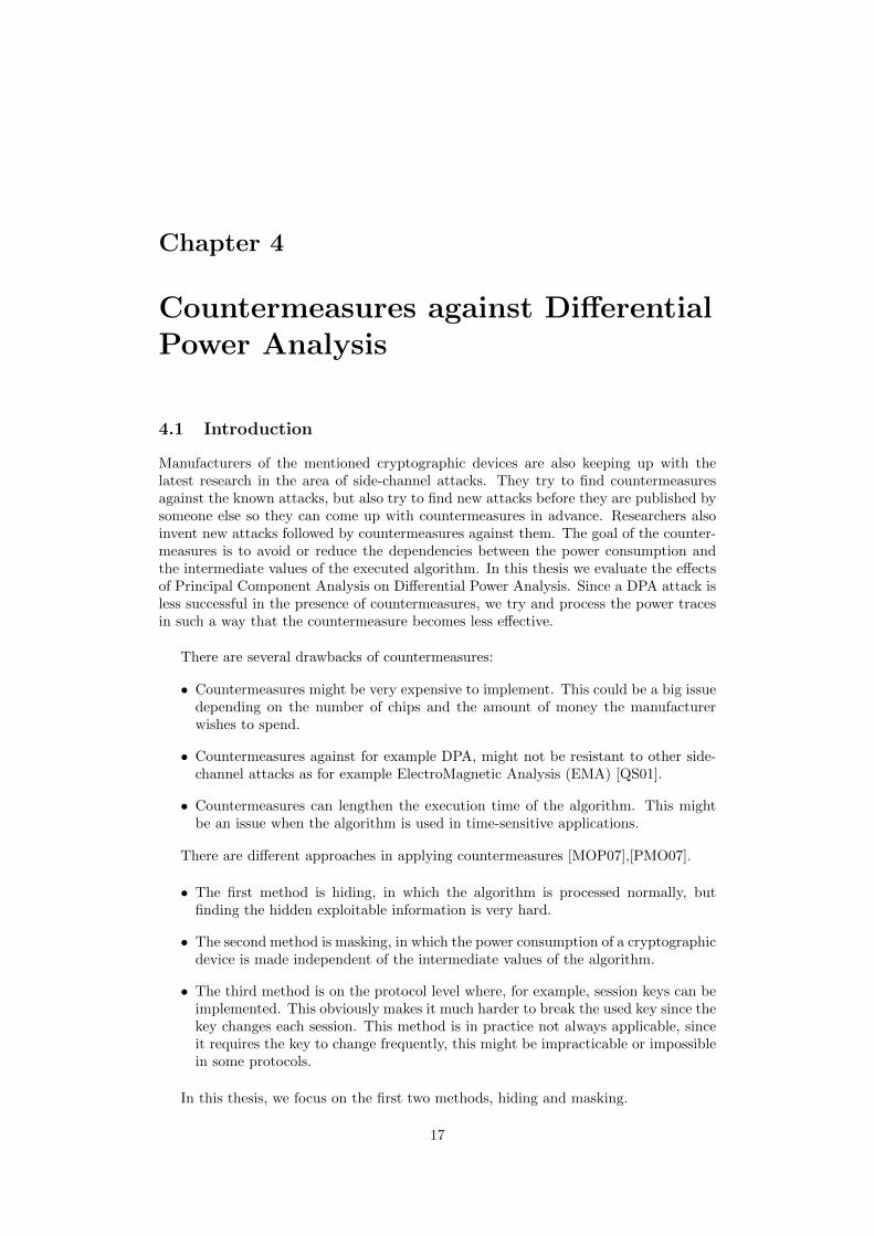
Manufacturers of the mentioned cryptographic devices are also keeping up with thelatest research in the area of side-channel attacks. They try to find countermeasuresagainst the known attacks, but also try to find new attacks before they are published bysomeone else so they can come up with countermeasures in advance. Researchers alsoinvent new attacks followed by countermeasures against them. The goal of the counter-measures is to avoid or reduce the dependencies between the power consumption andthe intermediate values of the executed algorithm. In this thesis we evaluate the effectsof Principal Component Analysis on Differential Power Analysis. Since a DPA attack isless successful in the presence of countermeasures, we try and process the power tracesin such a way that the countermeasure becomes less effective.
There are several drawbacks of countermeasures:
• Countermeasures might be very expensive to implement. This could be a big issuedepending on the number of chips and the amount of money the manufacturerwishes to spend.
• Countermeasures against for example DPA, might not be resistant to other side-channel attacks as for example ElectroMagnetic Analysis (EMA) [QS01].
• Countermeasures can lengthen the execution time of the algorithm. This mightbe an issue when the algorithm is used in time-sensitive applications.
There are different approaches in applying countermeasures [MOP07],[PMO07].
• The first method is hiding, in which the algorithm is processed normally, butfinding the hidden exploitable information is very hard.
• The second method is masking, in which the power consumption of a cryptographicdevice is made independent of the intermediate values of the algorithm.
• The third method is on the protocol level where, for example, session keys can beimplemented. This obviously makes it much harder to break the used key since thekey changes each session. This method is in practice not always applicable, sinceit requires the key to change frequently, this might be impracticable or impossiblein some protocols.
In this thesis, we focus on the first two methods, hiding and masking.
17

4. Countermeasures against Differential Power Analysis
4.2 Hiding
The main goal of hiding is to make the power consumption independent of the interme-diate values and independent of the operations that are performed. [MOP07] mentionstwo ways in which this can be achieved. The first is to make the power consumptionrandom so that a random amount of power is consumed each clock cycle. The secondway is to make sure that all operations and all data values consume the same power sothat each clock cycle the same amounts of power are consumed. These methods can beapplied in two ways.
The first way to implement these methods is to randomize the moments of time ofthe operations of the cryptographic algorithm. This creates a change in the time dimen-sion of the power consumption. This randomization can be created by inserting dummyoperations at randomized intervals at different locations when the cryptographic algo-rithm is executed. In order for this method to work, there needs to be a random numbergenerator which supplies the seeds for the number and location of dummy operations.Since DPA requires traces which are aligned, a DPA attack usually needs a lot moretraces in order to be successful when this method is applied.Another way to create randomization is to shuffle the operations of the cryptographicalgorithm. Take for example a DES encryption, where S-box lookups do not have to beperformed in a fixed order. Random numbers could be used to create a new sequence forS-box lookups for each encryption. This causes the power consumption to be randomfor each run. In practice, both of these methods are combined.
The second way the methods can be applied is to change the power consumptioncharacteristics of the performed operations and thus cause a change in the amplitude.If we lower the signal-to-noise ratio (SNR), performing a DPA attack becomes muchharder. The higher the signal-to-noise ratio is, the higher is the leakage.
SNR =V ar(Pexp)
V ar(Psw.noise+Pel.noise)[MOP07]
Where Pexp is the exploitable component of the power consumption, Psw.noise is theswitching noise and Pel.noise is the electronic noise.
This implies that if V ar(Psw.noise + Pel.noise) is raised, the signal-to-noise ratio de-creases. This means we could either increase the noise or reduce the signal. We couldincrease the noise by performing several operations in parallel, as, for example, hardwareimplementations of cryptographic algorithms do.Another way to decrease the SNR is to reduce the signal and thus make each operationconsume the same amount of power. If the power consumption of each cell is constant,the power consumption of the whole device is constant.
Examples of several logic styles which implement hiding are Sense Amplifier BasedLogic (SABL) [TAV02], Wave Dynamic Differential Logic (WDDL) [TV04] and Dual-rail Transition Logic (DTL) [MSS09].
Attacks on misaligned power traces are discussed in chapter 9.1. Our focus willbe on a countermeasure which introduces random delays. Since Principal ComponentAnalysis does not look at the time domain, but instead at the variance of samples, itcould potentially negate the effects of random delays.
4.3 Masking
Masking countermeasures can be implemented at the architecture level without chang-ing the power consumption characteristics of the cryptographic device. Masking causes
18

4.3. Masking
the power consumption to be independent of the intermediate values. Masking is basi-cally done by creating a random value for each execution which is called a mask. Thismask is then used to conceal the intermediate value by performing an operation on thetwo values, for example an exclusive-or (XOR) vm = v ⊕m or an arithmetic operationvm = v + m (mod n) depending on the used cryptographic algorithm. Since vm andv are uncorrelated, and only vm and m are processed, the power consumption remainsuncorrelated to v. One must be careful in defining the number of different masks. Us-ing many different masks obviously decreases the performance. Using just one maskhowever is also not advisable, since when two masked values are XOR’ed together, oneshould be sure that the result is masked as well [MOP07].It is important that each intermediate value needs to be masked. At the end of thealgorithm, there needs to be an unmask step in order to obtain the ciphertext.
It is also possible to perform masking at the cell level, which uses the same basicprinciples as mentioned above. Examples of masked logic styles are Masked Dual-railPrecharge Logic (MDPL) [PM05] and Random Switching Logic (RSL) [SSI04]. Sincemasked implementations are not considered in this thesis, the interested reader is advisedto read [MOP07].
19


Chapter 5
Principal Component Analysis(PCA)
5.1 Introduction
Principal Component Analysis (PCA) is a technique which is widely used to reduce thenoise or the dimensionality in a data set, while retaining the most variance, by findingpatterns within it. The origin of PCA can be traced back to Pearson [Pea01], but themodern instantiation was formed by Hotelling [Hot33].PCA searches for linear combinations with the largest variances, and divides them intoPrincipal Components (PC) where the largest variance is captured by the highest com-ponent in order to extract the most important information. PCA is used in manydifferent domains such as gene analysis and face recognition. An example of PCA andthe applications of PCA to side-channel analysis will be given.
Figure 5.1: A plotted data set with bothof its principal components [Jol02]
Figure 5.2: Plot of the transformed dataset of figure 5.1 with respect to bothprincipal components [Jol02]
In order to illustrate the workings of PCA, we give a small example for a two-dimensional (x,y) data set with 50 observations [Jol02]. In figure 5.1 a plot of this dataset is given. The first principal component is required to have the largest variance. Thesecond component must be orthogonal to the first component while capturing the largestvariance within the dataset in that direction. These components are plotted in figure5.1. This results in components sorted by variance, where the first component capturesthe largest variance. If we transform the data set using these principal components, theplot given in figure 5.2 will be obtained. This plot clearly shows that there is a larger
21

5. Principal Component Analysis (PCA)
variation in the direction of the first principal component.
When we apply this example to power measurements, we have a data set where thedimensionality is equal to the number of samples and the number of observations isequal to the number of traces. This means that the number of Principal Componentswhich can be deduced from a power trace is equal to the number of samples.
5.2 Mechanics
As mentioned before, PCA is mostly used when trying to extract interesting informationfrom data with large dimensions. Power traces usually have large dimensions, and onewould like to find the information of the key leakage within them. This could make theman ideal target for Principal Component Analysis. In order to make such an analysis, afew steps have to be performed [Smi02].
• First, the mean from each of the dimensions n of the traces Ti, is calculated in avector Mn.
Mn =
T∑i=1
Ti,n
n
This mean Mn must be subtracted from each of the dimensions n for each trace Ti.
Ti,n = Ti,n −Mn
• Construct the covariance matrix Σ. A covariance matrix is a matrix whose (i, j)thelement is the covariance between the ith and jth dimension of each trace. Thismatrix will be a n∗n matrix where n is equal to the number of samples (dimension)of the power traces. This means that the calculation time increases quadraticallyrelative to the number of samples. This is also the main drawback of PCA.
The covariance for two dimensions X and Y is defined as follows:
Cov(X,Y ) =
∑n
i=1(Xi−X)(Yi−Y )
n−1
Using the formula for the covariance, the covariance matrix is defined as follows:
Σn∗n = (ci,j , ci,j = Cov(Dimi, Dimj))
Where Dimx is the xth dimension.
• Then calculate the eigenvectors and eigenvalues of the covariance matrix.
Σ = U ∗ Λ ∗ U−1
22

5.3. Choosing the right number of principal components to keep
Where the eigenvalue matrix Λ is diagonal and U is the eigenvector matrix of Σ.These eigenvectors and eigenvalues provide information about the patterns in thedata.
The eigenvector corresponding to the largest eigenvalue is called the first principalcomponent, this component corresponds to the direction with the most variance.Since n eigenvectors can be derived, there are n principal components. They haveto be ordered from high to low based on their eigenvalue. Afterwards, the firstprincipal component represents the largest amount of variance between the traces.
• Choose p components which one wishes to keep, and form a matrix with thesevectors in the columns. This matrix is called the feature vector.
With this feature vector of length p, two things can be done. The original data canbe transformed to retain only p dimensions, or the noise of the original data set can bereduced using some components while keeping all n dimensions. These applications arediscussed in section 5.4.
5.3 Choosing the right number of principal components to keep
Choosing the right number of principal components to keep is essential in order to gainoptimal results. In chapter six of [Jol02] multiple ways are described in order to derivethe number of components which should be kept. A summary of two of these methodswill be given.
5.3.1 Cumulative percentage of total variation
For this method, a threshold is defined as the percentage of total variation one wishes tokeep. The amount of components which should be kept is then defined as the smallestamount for which this threshold is exceeded.By defining the percentage as e.g. 90%, the resulting data set contains only 90% of thetotal variation, but the number of components has been reduced. Choosing the rightpercentage is dependent on the application.
5.3.2 Scree test
The second method is to plot the eigenvalues according to their size. This is the so-calledscree test [Cat66]. The name is derived from the similarity of the typical shape of theplot (see figure 5.3) to that of the accumulation of loose rubble, or scree, at the foot ofa mountain slope [Jol02].Only the components which are before the point where the plot turns from a steep intoa flat line (elbow) are kept. This way you expect the components which are thrownaway not to contain much useful information with respect to the larger components.
Figure 5.3: A plot of some sample eigenvalues
23
5. Principal Component Analysis (PCA)
5.4 Applications for side-channel attacks
Principal component analysis can be used in two ways, a PCA transformation (whichcan also be used to reduce the dimensions) and a noise reduction of a dataset.
5.4.1 PCA transformation
Power traces used for DPA usually have large dimensions (a high number of samples)which makes calculations computationally intensive. It would be a great improvementif these dimensions can be reduced without removing much relevant data. This mightimprove the computation time of DPA. PCA can be used to reduce the dimensionalityof the dataset by removing the samples which do not relate to the leakage of the secretkey after a transformation in terms of lines that describe the relationship between thedata the best. The feature vector U and the original data X can be used to derive thisreduction. If we transpose the feature vector, we get the eigenvectors in the columns.By multiplying this vector with the transposed mean-adjusted data, we get the trans-formed data set X. This is the original data in terms of the chosen principal components.
Y = UT ∗XT = (X ∗ U)T
X = Y T = ((X ∗ U)T )T = X ∗ U
5.4.2 Noise reduction
If we do not want to remove dimensions, but instead would like to reduce the noise in thetraces in order to keep only the most relevant information, we can use the chosen Prin-cipal Components to retain only the most important information. If we choose to retainall principal components, this method returns the original data since no information isdiscarded. Normally, one would remove the components which contribute to the noise.The first step is the same as in a transformation, the feature vector U is transposed andmultiplied with the transposed mean-adjusted data X. Then, in order to get the originaldata X back, this matrix is multiplied by the feature vector. In order to get the rows andcolumns correct, we transpose this final matrix Z. Because we want the original databack, we have to add the mean, which was subtracted in the first step, to each dimension.
Y T = X ∗ UZ = U ∗ (X ∗ U)T = U ∗ UT ∗XT = XT
X = ZT = (XT )T = X
24
Chapter 6
Experiments
6.1 Introduction
We would like to study the effect of PCA on DPA attacks. Since there are different waysof implementing a cryptographic algorithm, we need power measurements from differ-ent sources. In this thesis we use simulated power measurements, power measurementstaken from smartcards (a software DES and a hardware DES) and power measurementstaken from a SASEBO-R (hardware AES-256).
We created a measurement setup to take measurements from these different sources.The following sections describe the setup and the used method of acquiring power traces.
6.2 Measurement setup
In order to measure power traces of a smartcard or a SASEBO, a few components arenecessary. This includes hardware and software components. Figure 6.1 shows ourmeasurement setup.
6.2.1 Hardware
Taking measurements requires the following hardware components.
• Power tracer Riscure B.V. developed an advanced smartcard reader which con-tains e.g. a trigger for the oscilloscope and a software-controlled smart card supplyvoltage. The power traces is used to measure the power consumption. It also en-hances the signal to noise ratio of the output which can then be measured by anoscilloscope.
• Picoscope A Picoscope is a PC-based digital oscilloscope which is used to recordthe power measurement traces and send them to the PC for further processing. Inour setup, the Picoscope 52031 is used.
• Filters Two electronic filters were provided for use within this project. Thesefilters process the signal which is passing through in order to reduce noise, andmake it easier to analyze the measured traces. We make use of a 50 Ohm, 48Mhz lowpass filter which passes low-frequency signals, reduces the amplitude ofhigh-frequency signals and reduces aliasing. Also we make use of an impedancefilter.
• Computer A computer is necessary to control the hardware and store and vi-sualize the acquired measurements. It is important to have sufficient computingpower since analysing traces usually requires a lot of computations.
1http://www.picotech.com/picoscope5200.html
25

6. Experiments
Figure 6.1: Our measurement setup, next to the laptop, one can see the oscilloscopewith the power tracer on top.
• Smartcards We need to have cryptographic devices to perform out measurementson. We make use of two smartcards provided by Riscure B.V., which are SampleType 2 which contains a software implementation of DES and Sample Type 8which contains a hardware implementation of DES.
• Side-channel Attack Standard Evaluation Board (SASEBO) A SASEBOboard is a device which is used to evaluate side-channel attacks. It is a pro-grammable cryptographic hardware device which allows power and electromag-netic measurements. The board can be programmed using a Field-ProgrammableGate Array (FPGA) in order to switch typical countermeasures on or off to testside-channel attacks. In this project, power traces acquired from an AES encryp-tion on the SASEBO-R are used [Res08].
6.2.2 Software
In order to process and analyse traces, we need to visualize them on the PC. Riscuredeveloped an application in order to process them.
• Inspector 4.1 Riscure B.V. developed an application named ”Inspector”. Theused version is 4.1. Inspector is designed as a side-channel analysis tool which canbe used to acquire, browse, inspect and analyse samples. These samples can bee.g. power measurements or electromagnetic measurements. Inspector containsmodules which allow filtering, alignment and analysis of signals. There are quite afew supported algorithms (e.g. DES, AES and ECC) for which DPA attacks canbe performed.
26

6.3. Obtaining traces
Because of these properties, Inspector is used for the acquisition and analysis ofpower traces within this project.
6.3 Obtaining traces
Obtaining power traces from a target device takes a couple of steps. This section de-scribes how traces can be obtained from smartcards and from a SASEBO.
6.3.1 Smartcard
Obtaining a traceset of the DES encryption of a typical smartcard is done by usingInspector. The module to acquire DES traces contains some adjustable options in orderto get traces of the best quality. The most important ones for the oscilloscope are thesample frequency, the number of samples and the delay. The sample frequency definesthe number of samples per second. The resulting measurement will be more detailedif this frequency is higher. Lower sample frequencies are for example used to createan overview of a full encryption over a longer period of time. If a delay is given, theoscilloscope will start measuring the given amount of time after the trigger signal.
Further, we can insert some parameters for the power tracer. These parameters in-clude a delay, but also the number of traces one would like to obtain. Also we can adda module which should be applied to each trace in a chain. In our acquisitions, we usethe ”resample” module to resample the power traces. The power traces we take fromsample card 2 are resampled to 4 Megahertz (MHz) which is equal to the external clockfrequency. We do this resampling step because we want to compress our measurementsin order to reduce the number of samples. The clock frequency is the lower limit sincewe would like to have each key processed in a different sample. If we resample to a lowerfrequency, the key information might not be in its own sample. Sample card 8 has aninternal clock frequency around 31 MHz. Further we can tweak the gain, the offset andthe voltage of the power tracer in order to get the best measurements.
The first step one has to take is to find the moment in time where the first roundof the DES encryption starts. In order to find this position, the first measurement wetake contains all DES rounds. Since we just need an overview to find the first round, weuse a low sampling rate (e.g. 67.5 Megasamples per second), obtain 3.5 million samplesand resample them to 4 MHz. The computer is then used to send a specific amountof random plaintexts, depending on the amount of traces we need, to the card. Thecard will encrypt each plaintext, and send the ciphertext back. The oscilloscope is usedto record the power consumption of these encryptions, and sends the data back to thecomputer.
An example of such a trace is given in figure 6.2. In this trace, all three roundsof the 3-DES encryption of the plaintext and the processing of the ciphertext can bedistinguished.
Figure 6.2: A full 3-DES encryption acquired from sample card 2
27

6. Experiments
We only need measurements of the first round of the algorithm to do a DPA attackon all S-boxes. Since we would like to keep the number of samples as small as possiblein order to keep the computational requirements as low as possible, we roughly needto find the position where the first round starts, and record from there. The powertracer can give a trigger signal to the oscilloscope after a specified delay so only therelevant data will be measured. For the power measurements of the first round, we usea higher sample frequency of 125 Megasamples per second in order to get more detailedinformation. Also, we resample the obtained traces to 4 MHz.
Following these steps will provide us with usable power measurements for our exper-iments.
6.3.2 SASEBO
Taking traces from a SASEBO is a bit different as compared to taking traces from asmartcard. The first thing we need is a power supply in order to power the SASEBO.Then we need to connect the SASEBO to a computer in order to send commands. Somesoftware to communicate with the SASEBO is also needed. This way one can sendcommands and install software on the chip. Same as for the smartcards, one needs anoscilloscope to visualize the power consumption.One also needs two power probes in order to measure the power consumption. Theseprobes should be placed on two pins on the SASEBO.When these initial steps are finished, one can use Inspector to send plaintexts to theSASEBO which will then be processed. The power probes can measure the used powerand send this information to the oscilloscope which sends the measurements to the com-puter.
We were not able to get a power supply on the Radboud University within time andthe power probes were in use at Riscure. This meant that we could not take our ownmeasurements.Yang Li and Kazuo Sakiyama were so kind to provide us with measurements which weretaken from AES-256 encryptions on a SASEBO-R. We use these measurements in ourexperiments.
28

Chapter 7
Principal Component Analysis andnoise reduction - Experiments
7.1 Introduction
One of the properties of PCA is that it can be used to reduce the noise of a traceset.We wish to investigate the effect PCA has on DPA. Since DPA inspects the relationshipbetween the measured power and the hypothetical power, reducing the noise in a trace-set might have a positive or negative effect on finding the secret key by performing DPA.
The experiments were performed using a custom made Java implementation of PCAin Inspector. See appendix A for a full listing. The code was verified by checking if theresults of a noise reduction on the dataset which is used in [Smi02] match their results.
In simulated DES encryption there is no simulation of things like the processing ofthe plaintext. Also, there is no noise, which means that the measurements are perfect.In order to evaluate how PCA performs on a noise-less traceset, we also consider sim-ulated traces. We expect there will be differences between simulated DES encryptiontraces and real DES encryption traces due to the difference in noise.
We suspect that some Principal Components capture the variance of the key leakageof the different S-boxes. If we only keep those Principal Components, and do not usethe others, we should be able to reduce the noise in the original signal. Since the largestvariance is captured in the highest Principal Components, we suspect that, if there is nonoise in the measurements, the information of the key leakage should be in these largestcomponents. If there is a lot of noise with a high variance, according to the propertiesof PCA, the information of the key leakage should be within the smaller components.
We implemented the PCA module in such a way that its output contains both theoriginal traces with their noise reduced, all of the Principal Components and a plot ofthe eigenvalues in order to evaluate the Principal Components for interesting results.
7.2 Simulated traceset (DES)
The first traceset we consider is created by making use of a module in Inspector whichcan simulate DES encryption traces using a known plaintext and a known key. The sim-ulated tracesets which are used in the following experiments all have the artificial keyleakage in sample 0-7, 20-27 and 120-127. We create a traceset of 1000 traces of a sim-ulated DES encryption with 256 samples per trace. This simulated traceset contains akey leakage at a known position which makes it easy to measure the success of the attack.
29

7. Principal Component Analysis and noise reduction - Experiments
Inspector contains a module named ’DESAnalysis’ which performs a DPA attack ona given traceset. It follows the same steps as explained in section 3.4. After performingthese steps, the module outputs correlation traces for each S-box and each candidate subkey using Correlation Power Analysis. This results in 8 ∗ 64 = 512 output traces. Thesecorrelation traces are scanned for the highest peak, which indicates the correctness ofthe sub key. This module is used to measure the effectiveness of the PCA transformationby looking at the correlation for the highest peak.
7.2.1 Experiments
Our first experiment is based on a simulation of power measurements of a DES encryp-tion without any noise. Since there is no noise, we expect the DPA information to havethe largest variance. Since Principal Component Analysis captures the sample with thelargest variance in the same component, we expect the largest eight Principal Compo-nents to capture the key information for each S-box.
Since we also would like to see how a traceset with noise compares, we added somerandom noise to each sample of this traceset, and did some experiments with these.If there is a lot of noise, we expect the key leakage to be present in smaller PrincipalComponents.
7.2.1.1 Simulated traces without noise
Our first experiment is based on a simulation of power measurements of a DES en-cryption without any noise. Figure 7.1 shows a sample power measurement of thissimulation.
Figure 7.1: A simulated DES encryption trace without noise
Performing a noise reduction with PCA using all Principal Components on thesesimulated traces shows some interesting results. The first thing we do is inspect thePrincipal Components. Since we kept all of them, there was no noise reduced from theoriginal traceset. Inspecting the values of the Principal Components shows clearly thatthe first eight Principal Components show a large variation at the spots where the keyleakage is in the traces. Since the key is leaked in three locations, three groups of peakscan be spotted (0-7, 20-27 and 120-127). At all the other locations, much less variationcan be seen. Figure 7.2 shows the first Principal Component, all 7 following PrincipalComponents are visually roughly equal to this trace. It looks like each component showsthe variation of the key leakage of one S-box. All the other Principal Components rep-resent more variance in different places. An example of such a component is component9 which is shown in figure 7.3.
As we expected, since there is no noise, the samples with the largest variance capturethe variance of the key leakage. Since these samples have the largest variance, they arecaptured by the first eight Principal Components. The 9th component captures the dataorthogonal to the 8th component with the largest variance left. Since the key leakagehas already been captured by the first eight components, this data will not be capturedby smaller components.
30

7.2. Simulated traceset (DES)
Figure 7.2: First Principal Component of a simulated DES encryption trace withoutnoise
Figure 7.3: Ninth Principal Component of a simulated DES encryption trace withoutnoise
7.2.1.2 Simulated traces with artificially added noise
Since there is no noise in this simulation, and real measurements do contain noise, weperform the same experiment on the same traceset where we add some random noise.The simulation module allows one to provide a noise level, this level is the standarddeviation of the normal distributed noise. We create a traceset with noise level 10 tosimulate 1000 traces with 256 samples. The signal level is equal to the variance of thesignal. We calculate the distribution of the values for sample 0 (where the first keyleakage is). There are 57 traces with value 0, 249 traces with value 1, 383 traces withvalue 2, 241 traces with value 3 and 70 traces with value 4. This means that the meanvalue for this sample is 2.018. We now calculate the difference of the mean for eachvalue and square these. Adding these values and dividing by 1000 now gives us the vari-ance, which is equal to 0,997676. Since the signal level is the variance of the signal, itis roughly equal to 1. This means that a noise level of 10 lowers the SNR with a factor 10.
It is important to note that a DPA attack on this traceset does not rank the correctkey the highest due to too much noise.
We perform PCA using a noise reduction on this obtained traceset. Inspecting thePrincipal Components clearly shows that, again, the first eight Principal Componentscapture the variance of the samples which contain the key leakage.
The first Principal Component is plotted in figure 7.4. The peaks show the varianceon the positions where the key leakage is and not much variance for the other samples.Since we are only interested in the samples where the leakage is, and wish to reduce thenoise as much as possible, it makes sense to try and reduce the noise by using only thefirst eight Principal Components in the PCA calculation. The noise-reduced tracesetusing only these eight components shows clear peaks at the locations which contain theleakage, see figure 7.5. This was to be expected since we chose the components basedon the peaks for the samples which contain the key leakage and a small variance for theother samples.
The right position of the key leakage can now easily be spotted in the traces, evenfrom simulated traces with a very high noise level. We are not able to find the correct
31
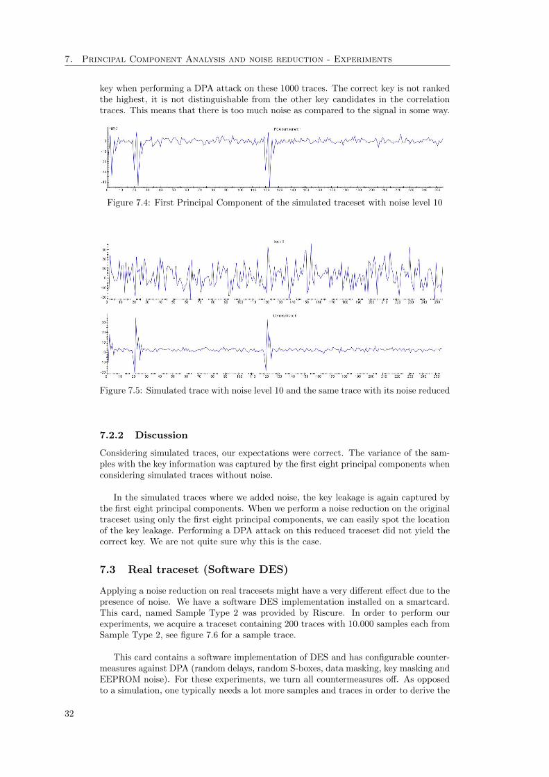
7. Principal Component Analysis and noise reduction - Experiments
key when performing a DPA attack on these 1000 traces. The correct key is not rankedthe highest, it is not distinguishable from the other key candidates in the correlationtraces. This means that there is too much noise as compared to the signal in some way.
Figure 7.4: First Principal Component of the simulated traceset with noise level 10
Figure 7.5: Simulated trace with noise level 10 and the same trace with its noise reduced
7.2.2 Discussion
Considering simulated traces, our expectations were correct. The variance of the sam-ples with the key information was captured by the first eight principal components whenconsidering simulated traces without noise.
In the simulated traces where we added noise, the key leakage is again captured bythe first eight principal components. When we perform a noise reduction on the originaltraceset using only the first eight principal components, we can easily spot the locationof the key leakage. Performing a DPA attack on this reduced traceset did not yield thecorrect key. We are not quite sure why this is the case.
7.3 Real traceset (Software DES)
Applying a noise reduction on real tracesets might have a very different effect due to thepresence of noise. We have a software DES implementation installed on a smartcard.This card, named Sample Type 2 was provided by Riscure. In order to perform ourexperiments, we acquire a traceset containing 200 traces with 10.000 samples each fromSample Type 2, see figure 7.6 for a sample trace.
This card contains a software implementation of DES and has configurable counter-measures against DPA (random delays, random S-boxes, data masking, key masking andEEPROM noise). For these experiments, we turn all countermeasures off. As opposedto a simulation, one typically needs a lot more samples and traces in order to derive the
32
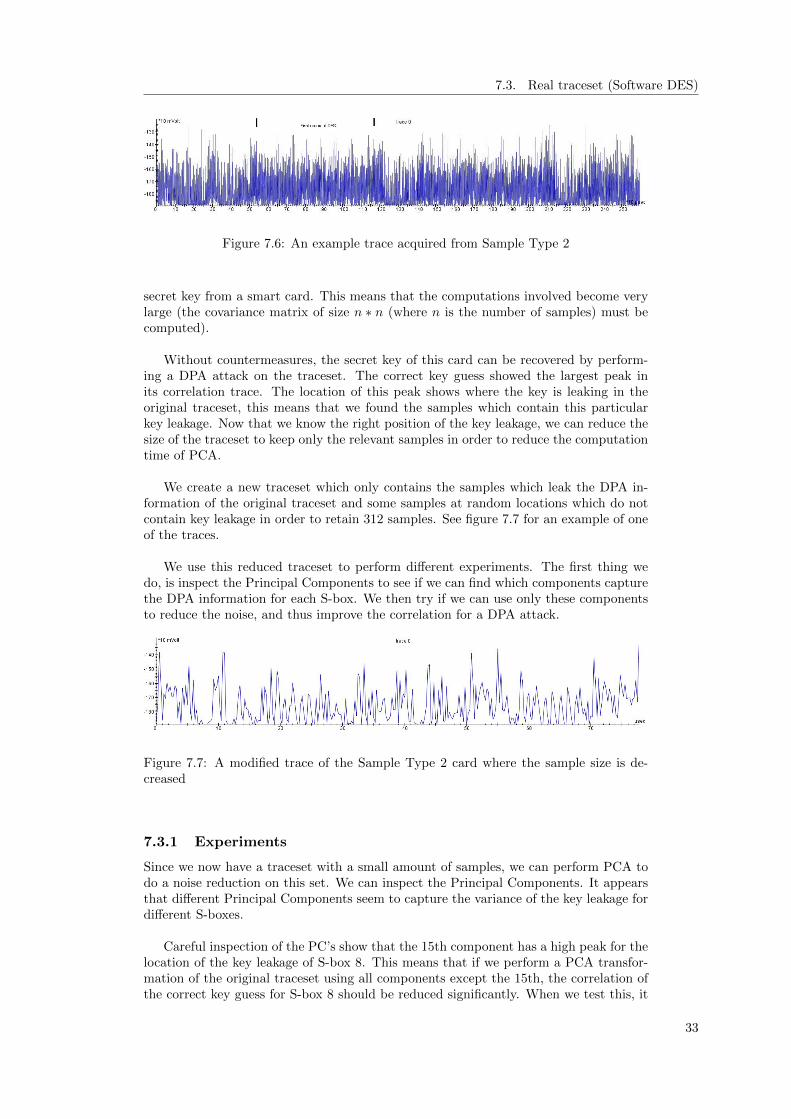
7.3. Real traceset (Software DES)
Figure 7.6: An example trace acquired from Sample Type 2
secret key from a smart card. This means that the computations involved become verylarge (the covariance matrix of size n ∗ n (where n is the number of samples) must becomputed).
Without countermeasures, the secret key of this card can be recovered by perform-ing a DPA attack on the traceset. The correct key guess showed the largest peak inits correlation trace. The location of this peak shows where the key is leaking in theoriginal traceset, this means that we found the samples which contain this particularkey leakage. Now that we know the right position of the key leakage, we can reduce thesize of the traceset to keep only the relevant samples in order to reduce the computationtime of PCA.
We create a new traceset which only contains the samples which leak the DPA in-formation of the original traceset and some samples at random locations which do notcontain key leakage in order to retain 312 samples. See figure 7.7 for an example of oneof the traces.
We use this reduced traceset to perform different experiments. The first thing wedo, is inspect the Principal Components to see if we can find which components capturethe DPA information for each S-box. We then try if we can use only these componentsto reduce the noise, and thus improve the correlation for a DPA attack.
Figure 7.7: A modified trace of the Sample Type 2 card where the sample size is de-creased
7.3.1 Experiments
Since we now have a traceset with a small amount of samples, we can perform PCA todo a noise reduction on this set. We can inspect the Principal Components. It appearsthat different Principal Components seem to capture the variance of the key leakage fordifferent S-boxes.
Careful inspection of the PC’s show that the 15th component has a high peak for thelocation of the key leakage of S-box 8. This means that if we perform a PCA transfor-mation of the original traceset using all components except the 15th, the correlation ofthe correct key guess for S-box 8 should be reduced significantly. When we test this, it
33

7. Principal Component Analysis and noise reduction - Experiments
appears to be the case. Where the correlation for the correct key for S-box 8 was 0.7191in the original traceset, performing a PCA noise reduction using all Principal Compo-nents except the 15th, yields a correlation for the correct key for S-box 8 of 0.5257. Thecorrelation for the correct key guess for all other S-boxes remained roughly the same.This means that, in order to improve the correlation for the key guess of S-box 8, weshould keep all components which capture a part of the variance for the sample of thekey leakage.
We perform PCA by making use of different numbers of Principal Components inorder to reduce as much noise as possible to try to improve the correlation for the correctkey guess for all S-boxes.Since the largest amounts of noise are captured by the largest Principal Components,we perform a noise reduction without using some of these largest components. We trydifferent numbers. A PCA noise reduction using all components except the largest 25seems to yield good results. When we perform a DPA attack on the noise-reduced traces,the correlation for the correct key for most S-boxes, except S-box 4 and 8, improves whencomparing the results to a DPA attack on the original traceset. The correlation for S-box4 and 8 becomes worse. The correlation for the correct key guess for S-box 1 improvesfrom 0.6592 before the noise reduction to 0.6738 after the noise reduction. This meansthat the relevant DPA information for S-box 1, 2, 3, 5, 6 and 7 is not captured by thelargest 25 components.
7.3.1.1 S-box 4 and 8
Careful analysis shows that the variance for the key leakage for S-box 4 and 8 is presentin larger PC’s than for the other 6. In this case, for S-box 4 and 8, the largest varianceis present in some PC’s between the 6th and the 32th. Since we did not use the first25 PC’s, this explains why the key distinction becomes worse. This also means that thevariance in the leakage of those S-boxes is larger than for the other six.Since the information for S-box 4 and 8 is present in larger PC’s, this means that theirvariation is larger. We can not explain this difference in behaviour for S-box 4 and 8 asopposed to the other S-boxes. We inspected the source code of the DES implementationon the card but could not find any difference between the implementation of the S-boxes.Our best guess would be that the assembly code contains some differences which mightexplain this behaviour.
7.3.1.2 Noise
The information for the other 6 S-boxes was captured somewhere after the 25th Princi-pal Components. This means that the components from 1 until 25 capture informationwith more variation than those S-boxes, which should be noise. In order to test this,we add large amounts of random noise to a number of samples (30). If the variation ofthis noise is larger than the variation of the key information, we expect that it shouldbe captured by some of the first Principal Components and thus that the relevant DPAinformation will be captured by smaller Principal Components than before. We imple-mented and used a module which does exactly this. We perform the same experimentas before on this new traceset, and check in which components the information is now.It appears that the information is now present in the Principal Components which arelarger than 55. This means that, as expected, adding noise with a large variation shiftsthe DPA information to smaller components.
In our experiment with the simulated traces, this phenomenon did not appear, thekey information did not shift to smaller components. This was due to the case that weadded noise to each of the samples in those traces instead of only 30 of them. PCAcaptures the components with the largest variance in the largest components. Sincethe noise was added to each sample, the samples with the key leakage, which already
34

7.4. Real traceset (Hardware DES)
contained the largest variance, still contain the largest variance. If noise with a largevariance is introduced to some samples, those samples gain a much larger variance thanthe rest which is unaffected. This means that in this case, the samples to which thenoise was added will be captured in a larger component than before.
7.3.2 Discussion
Because not all information is present in the same components, it would be best if allPC’s which have a high contribution to the variance of the key leakage of one singleS-box remain and the others are removed. The biggest problem is that if we removethe rest of the Principal Components, the correlation of the right key guess for otherS-boxes becomes much lower. This leads to the conclusion that, in order to get theoptimal results, the PCA filter should be applied eight times on the original traceset,once for each S-box and its most relevant components.
A prerequisite for this method is that the position of the key leakage should be ap-proximately known in order to find which PC’s must be retained. The best results areobtained when the position is precisely known since this will allow removing the largestpart of irrelevant Principal Components. An easy way to find the correct key leakagesample is to obtain a card of the same type with a known key which might be possiblein lab situations. It is much easier to find the places of key leakage if the key is known,since this can be checked. If we are able to derive this key, and know at which samplesthe key is leaking, we know which components we should keep in order to improve theDPA attack.
We can conclude that the largest Principal Components capture the largest partof the noise for this traceset since adding noise with a large variance shifted the DPAinformation to smaller Principal Components.
7.4 Real traceset (Hardware DES)
The main difference between a hardware and software DES implementation is that inhardware, one DES round can be computed in one single clock cycle as opposed tosoftware where one round is computed in many clock cycles. This attribute makes theimpact of PCA possibly different as compared to the results before. Performing a suc-cessful DPA attack on a hardware DES typically requires a lot more traces as opposedto software DES since there is a lot more noise. A lot more switching is done in thesame amount of time as compared to software since all S-boxes are calculated in parallel.Because of these larger amounts of noise, we expect the DPA information to be capturedin smaller Principal Components than with software DES.We expect that the results of a noise reduction are the same as before but since theS-boxes are used in the same clock cycle, keeping the correct PC’s should improve thecorrelation for the key guess for each S-box.
To find if there is a difference between tracesets obtained from software and hardwaredevices, the same experiments we performed before are performed on a traceset whichwe obtain from a hardware device performing a DES encryption, see figure 7.8.
7.4.1 Experiments
We acquire a traceset of 48852 traces with 1232 samples each from Sample Type 8 whichcontains a hardware DES implementation. A DPA attack can successfully recover thekey from this traceset and shows us the location where the key is leaked which is sample518. Since we now know the location of the key leakage, we can reduce the amount of
35

7. Principal Component Analysis and noise reduction - Experiments
Figure 7.8: A power trace acquired from a hardware DES encryption by Sample Type 8
samples which we use for the PCA calculation.
We create a new traceset which only contains samples 400 until 712 in order to keep312 samples which makes the calculations less time consuming.
We use this smaller traceset to perform a noise reduction using PCA retaining dif-ferent numbers of principal components. It appears that the best results are obtainedwhen we remove the first 50 components. The correlation rises from 0.0782 for thecorrect key guess for S-box 1 on the original traceset to 0.0842 on the noise-reducedtraceset. The correlation for the other S-boxes also improves. This means that thesefirst 50 components contain more noise than relevant data, and thus can be removed.
7.4.2 Discussion
We were able to improve the correlation for the correct key guess by removing somelarge components which captured the noise. It must be noted that, we can only applythis method if we know the location of the key leakage in order to reduce the amountof samples since this traceset contains too many traces and samples.We can conclude that the DPA information is captured by smaller Principal Componentsas with software. This is in line with our expectations, since the measurements whichwere taken from the hardware DES contain more noise than the measurements takenfrom the software DES.
7.5 SASEBO-R (AES-256)
To see how another cryptographic device would withstand PCA, we acquired sometraces from a SASEBO-R. Since our own measurement setup failed to work, we ac-quired a traceset from Yang Li and Kazuo Sakiyama of The University of Electro-Communications in Tokyo, Japan. They measured 5000 power traces with 1000 samplesof an AES encryption on a SASEBO-R without any countermeasures. A sample traceis shown in figure 7.9.
Figure 7.9: A power trace acquired from a SASEBO AES-256 encryption
Since we want to find out if noise reduction has any beneficial effects on this traceset,we try the same experiment as with the other tracesets.
36

7.6. How many and which components should be kept using power traces
The first thing we do is perform a DPA attack on the original traceset. We are ableto find the correct key for S-box 1 with a correlation of 0.1378. The second highestcorrelation, for a wrong key guess, is 0.0716.
7.5.1 Experiments
We try PCA transformations whilst removing a different number of Principal Com-ponents. For this traceset, if we remove 30 of the largest Principal Components, thecorrelation drops and the correct key is not ranked the highest anymore after performinga DPA attack. This means that the key information is present somewhere within thesecomponents, which means that the variation of the noise in this traceset is very small.
By trial and error, we tried to find the best results of a noise reduction. We foundthat removing the largest 2 Principal Components has the best results. This meansthat the some of the key information is present within the 3rd Principal Component.When we tried a noise reduction without the largest 2 components, the correlation forthe correct key guess increased to 0.1439 and the correlation for the wrong key guessdropped to 0.0648.
Since the smallest components should also contain noise, we try and remove someof these components which improved the correlation even more. When we use only the3rd until the 50th component (so remove the 2 largest and 950 smallest components),we can even increase the correlation to 0.1599. This means that the key information issomewhere within the 3rd until the 50th component.
7.5.2 Discussion
Performing a noise reduction on the SASEBO traces using the 3rd until the 50th Princi-pal Component shows an improvement for the correlation of the correct key guess. Thismeans that the noise was successfully reduced. The variation for the key leakage seemsto be fairly high compared to the variation of the noise since the DPA information iscaptured somewhere between the 3rd and 50th Principal Component.
7.6 How many and which components should be kept usingpower traces
As mentioned before there are multiple ways to select which components should be keptand which can be discarded. These methods do however assume that the componentswhich should be kept are always the largest. However, as we have seen with the ex-periments using power traces, it is not the case that the DPA information is present inthe largest Principal Components since this is usually noise. Since we need the DPAinformation, we have to find another way to choose which components should be kept.
We decide if a component is relevant by checking how much of the variance is cap-tured for the sample of the key leakage. We use the reduced traceset with 200 traceswith 312 samples taken from Sample Type 2 which we used in section 7.3 (figure 7.7)for this experiment. We try different thresholds to see if we can improve the correlationfor the correct key guess for the first S-box. We find the best threshold by experimenting.
Figure 7.10 shows the correlation values for the correct key guess for S-box 1 whendifferent thresholds are used to keep relevant components. As can be seen in the peak,the best threshold for this S-box is 0.07, which means that the Principal Componentswhich have a variance higher than 0.07 for the correct sample are kept. In this case, 35Principal Components are used in the transformation and the correlation improves from0.6592 to 0.7493. The figure also shows the correlation of the second key candidate.
37

7. Principal Component Analysis and noise reduction - Experiments
Figure 7.10: Graph showing the correlation after transformation of the original tracesetusing only the components which have a value of at least the threshold for the DPAinformation for S-box 1
This correlation also improves, but the correlation for the correct key guess improvesrelatively more which means there is an overall improvement.
Since this value might be different for other S-boxes, we redo this experiment forS-box 8 on the same traceset. Figure 7.11 shows this graph. As can be noted, there aremuch fewer Principal Components used for the same threshold as with S-box 1. Thehighest peak is around the value of 0.03. Here, 35 Principal Components are used forthe noise reduction. This is the same value as above which, by looking at the curve ofthe graph, leads us to believe that the best number of components to be kept for thissample card and for this number of samples is between 12 and 45 for each S-box.
In order to evaluate if this is the same for each traceset, we repeat this experimentfor a new traceset acquired from the same Sample Type 2 with a different key which alsocontains 200 traces with 312 samples per trace, and try the same thresholds as before.Figure 7.12 shows the results. The best result is a transformation which uses only thecomponents with a threshold of 0.1 for the correct sample for S-box 1. This resulted in atransformation using only 20 Principal Components. The correlation of the correct keyguess went up from 0.7050 before the noise reduction to 0.9375 after the noise reductionwhile the correlation for the second key guess only improved by a little.
7.6.1 Discussion
From these experiments, we can conclude that there is no ’magic’ threshold which wecan use to select the Principal Components which we would like to keep. It seems,
38
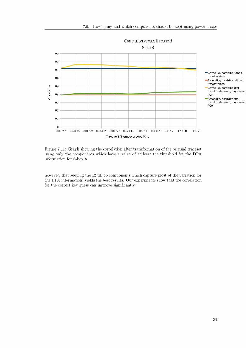
7.6. How many and which components should be kept using power traces
Figure 7.11: Graph showing the correlation after transformation of the original tracesetusing only the components which have a value of at least the threshold for the DPAinformation for S-box 8
however, that keeping the 12 till 45 components which capture most of the variation forthe DPA information, yields the best results. Our experiments show that the correlationfor the correct key guess can improve significantly.
39

7. Principal Component Analysis and noise reduction - Experiments
Figure 7.12: Graph showing the correlation after transformation of the original tracesetusing only the components which have a value of at least the threshold for the DPAinformation for S-box 1
40
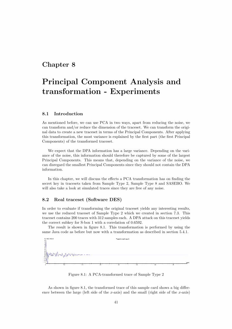
Chapter 8
Principal Component Analysis andtransformation - Experiments
8.1 Introduction
As mentioned before, we can use PCA in two ways, apart from reducing the noise, wecan transform and/or reduce the dimension of the traceset. We can transform the origi-nal data to create a new traceset in terms of the Principal Components. After applyingthis transformation, the most variance is explained by the first part (the first PrincipalComponents) of the transformed traceset.
We expect that the DPA information has a large variance. Depending on the vari-ance of the noise, this information should therefore be captured by some of the largestPrincipal Components. This means that, depending on the variance of the noise, wecan disregard the smallest Principal Components since they should not contain the DPAinformation.
In this chapter, we will discuss the effects a PCA transformation has on finding thesecret key in tracesets taken from Sample Type 2, Sample Type 8 and SASEBO. Wewill also take a look at simulated traces since they are free of any noise.
8.2 Real traceset (Software DES)
In order to evaluate if transforming the original traceset yields any interesting results,we use the reduced traceset of Sample Type 2 which we created in section 7.3. Thistraceset contains 200 traces with 312 samples each. A DPA attack on this traceset yieldsthe correct subkey for S-box 1 with a correlation of 0.6592.
The result is shown in figure 8.1. This transformation is performed by using thesame Java code as before but now with a transformation as described in section 5.4.1.
Figure 8.1: A PCA-transformed trace of Sample Type 2
As shown in figure 8.1, the transformed trace of this sample card shows a big differ-ence between the large (left side of the x-axis) and the small (right side of the x-axis)
41
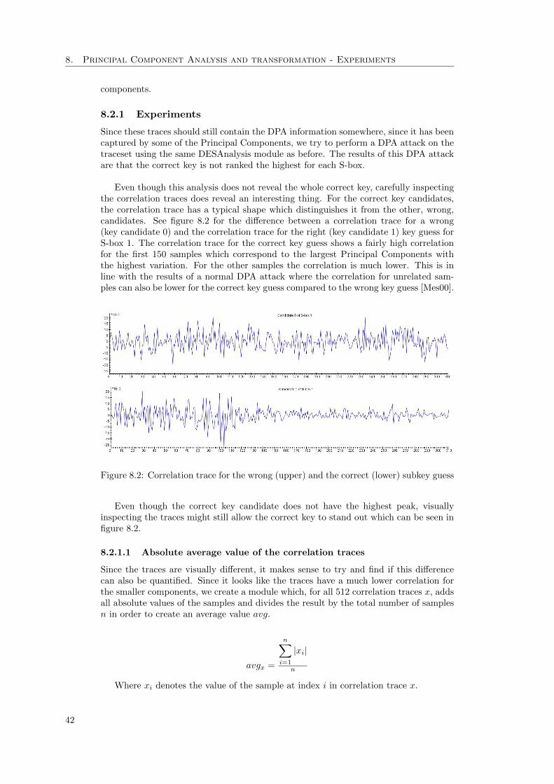
8. Principal Component Analysis and transformation - Experiments
components.
8.2.1 Experiments
Since these traces should still contain the DPA information somewhere, since it has beencaptured by some of the Principal Components, we try to perform a DPA attack on thetraceset using the same DESAnalysis module as before. The results of this DPA attackare that the correct key is not ranked the highest for each S-box.
Even though this analysis does not reveal the whole correct key, carefully inspectingthe correlation traces does reveal an interesting thing. For the correct key candidates,the correlation trace has a typical shape which distinguishes it from the other, wrong,candidates. See figure 8.2 for the difference between a correlation trace for a wrong(key candidate 0) and the correlation trace for the right (key candidate 1) key guess forS-box 1. The correlation trace for the correct key guess shows a fairly high correlationfor the first 150 samples which correspond to the largest Principal Components withthe highest variation. For the other samples the correlation is much lower. This is inline with the results of a normal DPA attack where the correlation for unrelated sam-ples can also be lower for the correct key guess compared to the wrong key guess [Mes00].
Figure 8.2: Correlation trace for the wrong (upper) and the correct (lower) subkey guess
Even though the correct key candidate does not have the highest peak, visuallyinspecting the traces might still allow the correct key to stand out which can be seen infigure 8.2.
8.2.1.1 Absolute average value of the correlation traces
Since the traces are visually different, it makes sense to try and find if this differencecan also be quantified. Since it looks like the traces have a much lower correlation forthe smaller components, we create a module which, for all 512 correlation traces x, addsall absolute values of the samples and divides the result by the total number of samplesn in order to create an average value avg.
avgx =
n∑i=1
|xi|
n
Where xi denotes the value of the sample at index i in correlation trace x.
42

8.3. Real traceset (Hardware DES)
We use this method to calculate the absolute average for samples 150 until 312 ofthe correlation traces, since we noticed a difference in behavior here.Figure 8.3 shows these average values for each correlation trace. The x-axis shows thekey guess for each S-box. This means the first 64 values correspond to the 64 subkeysof S-box 1, the second 64 values to the 64 subkeys of S-box 2 and so on. One candistinguish eight downward peaks, which correspond to the correct key guesses. Thismeans that the total correlation for all samples for the correct key guess is lower thanfor the wrong key guesses. This was to be expected by inspecting figure 8.2.
Figure 8.3: Absolute average value of each correlation trace for Sample Type 2
8.2.2 Discussion
From this experiment, we can conclude that the correlation trace for the correct key guessis different from the correlation trace for the wrong key guess. Where in a normal DPAattack one is looking for the highest peak, we have found a different approach by lookingat the correlation trace which is different from the rest. We proposed a method to do thisby comparing the average value of parts of the correlation traces. The correlation for thelower samples of the correct key guess was lower for the smaller Principal Componentsin this traceset. This means that the smaller Principal Components do not seem tocapture the variance for the key leakage.
8.3 Real traceset (Hardware DES)
After looking at software, we wanted to see how a hardware DES compares by perform-ing a PCA transformation.For our experiments, we use the same reduced traceset, acquired from Sample Type 8,as in section 7.4.1. This traceset contains 48852 traces and 312 samples. A DPA attackon this traceset yields the correct key for S-box 1 with a correlation of 0.0782 for S-box 1.
We expect the results of a PCA transformation to be the same is with a softwareDES. The DPA information will probably in some smaller principle components sincethere is more noise. This is in line with the results we found with our noise reductionexperiment.
8.3.1 Experiments
The first thing we do is transform the traceset by performing a PCA transformation.When we perform a DPA attack on this transformed traceset, the highest peak is notthe one for the correct key guess. This means the DPA attack failed. Visually inspect-ing the traces does not yield any differences between the correct and the wrong key guess.
Since these differences might be subtle, we try and take the absolute value of eachsample for each correlation trace, and plot these.
Figure 8.4 shows the trace with the peaks marked. These peaks correspond to thecorrect key guesses. The only S-box for which the key guess is not distinguishable is
43

8. Principal Component Analysis and transformation - Experiments
S-box 7. It is not clear why the correct subkey for S-box 7 is harder to find, but it is aknown ”feature” of this particular card.
Figure 8.4: Absolute average value for the correlation for each key guess for SampleType 8
8.3.2 Discussion
We were able to find the used key by calculating the absolute average value of thecorrelation traces. The total correlation for the correct key guess for each S-box is,on average, larger than for the wrong key guess. These results are the opposite of theresults we obtained with the software DES traces, where there was a downward peak.
8.4 SASEBO-R (AES-256)
We expect that the results for the SASEBO traces are in line with the other results sincethe power measurements have the same properties. This means that we should be ableto find the used key by calculating the absolute average value of the correlation tracesafter a DPA attack on the transformed traceset. The only difference is that AES-256 isused instead of DES, but this should not make a difference since we still use CPA whichalso works for AES.
We use the same traceset as used in section 7.5. A DPA attack on this traceset showsthe correct key with a correlation of 0.1378 for S-box 1.
8.4.1 Experiments
The first step we take is performing a PCA transformation on the SASEBO traceset.On this transformed traceset, we perform a DPA attack. This results in finding thecorrect key with a correlation of 0.1115 for S-box 1. This is a bit lower than on the orig-inal traceset. The correct key bytes are found within the first 10 Principal Componentswhich means that there is not much noise. This means that if we look at the absoluteaverage for the correlation traces for the first 10 samples, it should produce clear peaks.
Figure 8.5 shows the plot for the absolute average for the first 10 samples fromthe correlation traces. Since these power measurements are acquired from an AES-256encryption, 16 key bytes are used. Each key byte can have 256 values. This means thatthere are 16 ∗ 256 = 4096 correlation traces. One can clearly spot the 16 peaks whichcorrespond to each correct key guesses for each key byte.
8.4.2 Discussion
As expected, we were able to find the correct key in the transformed trace by looking atthe average value of the correlation traces. This is in line with the result for hardwareDES.
44
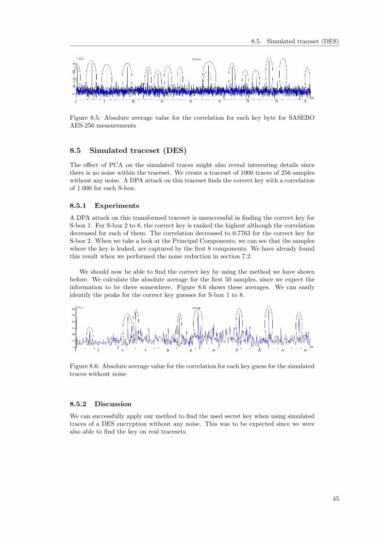
8.5. Simulated traceset (DES)
Figure 8.5: Absolute average value for the correlation for each key byte for SASEBOAES-256 measurements
8.5 Simulated traceset (DES)
The effect of PCA on the simulated traces might also reveal interesting details sincethere is no noise within the traceset. We create a traceset of 1000 traces of 256 sampleswithout any noise. A DPA attack on this traceset finds the correct key with a correlationof 1.000 for each S-box.
8.5.1 Experiments
A DPA attack on this transformed traceset is unsuccessful in finding the correct key forS-box 1. For S-box 2 to 8, the correct key is ranked the highest although the correlationdecreased for each of them. The correlation decreased to 0.7763 for the correct key forS-box 2. When we take a look at the Principal Components, we can see that the sampleswhere the key is leaked, are captured by the first 8 components. We have already foundthis result when we performed the noise reduction in section 7.2.
We should now be able to find the correct key by using the method we have shownbefore. We calculate the absolute average for the first 50 samples, since we expect theinformation to be there somewhere. Figure 8.6 shows these averages. We can easilyidentify the peaks for the correct key guesses for S-box 1 to 8.
Figure 8.6: Absolute average value for the correlation for each key guess for the simulatedtraces without noise
8.5.2 Discussion
We can successfully apply our method to find the used secret key when using simulatedtraces of a DES encryption without any noise. This was to be expected since we werealso able to find the key on real tracesets.
45


Chapter 9
Alignment
9.1 Introduction
As we have seen before, DPA attacks try to find the correlation between the hypothet-ical power consumption for the correct key hypothesis and the power consumption ata specific moment in time (where the calculated intermediate result is processed). Asshowed before, manufacturers have developed multiple countermeasures to make DPAattacks less successful. One of these countermeasures, which is an example of hiding, isto introduce random time delays during execution of the algorithm and thus misalignthe traces. Another source of misalignment is the start of the recording of the powerconsumption [MOP07] which should be exactly at the same time for each trace. Inpractice this is very hard to obtain. Also, the time interval between the trigger signaland the clock signal might not be constant, this means the recording does not alwaysstart at the same time. Figure 9.1 shows two traces which are misaligned.
As explained before, Principal Component Analysis looks at the variance within adata set, and captures the largest variance within the largest principal components.This means that PCA does not consider the time domain. The main requirement forDPA is that the traces should be aligned, and thus capture the same operation in thesame sample. A PCA transformation can be used to capture the samples with the keyinformation in the same principal component. This means that a DPA attack on thistransformed traceset, where the key information is captured within the same componentfor each trace, might be successful.
This means that one might be able to perform DPA on the transformed traceset anduse our absolute average method in order to find the correct key. In this chapter wedescribe the experiments we did with misaligned traces and the obtained results. Wewill also consider power measurements taken from a software DES encryption with acountermeasure which causes more misalignment due to random delays.
Figure 9.1: Two misaligned traces
There are three ways to deal with misalignment:
• Perform DPA analysis on the misaligned traces.
47

9. Alignment
• Align the power traces before performing the attack.
• Preprocess the power traces in order to reduce misalignment.
9.1.1 DPA on misaligned traces
A DPA attack on misaligned traces will still work, provided that one has enough traces.This usually requires much more traces than in the case when they are aligned. Obtain-ing such an amount of traces might be infeasible since the key is processed in differentpositions. It depends on the way the random delays are implemented how many extratraces are needed. When, for example, a random number is used to define the numberof delays for each execution, it depends on the distribution from where this number ischosen for how many traces are needed. If this random number is somewhere betweenone and 10, roughly ten times more traces are needed to get the same correlation sinceonly one in ten traces captured the same instruction at the same location.
9.1.2 Alignment before attack
The best way to process a misaligned traceset is by aligning the traces before mountinga DPA attack. Multiple methods have been proposed, of which three will be discussed.All methods cause the traces to be aligned after performing them. After alignment, thetraces shown in figure 9.1 look like the traces shown in figure 9.2.
Figure 9.2: The two traces from figure 9.1 after an alignment step
There are multiple different alignment methods of which two, static and elastic[vWWB] alignment, will be discussed here.
9.1.2.1 Static alignment
Static alignment is a process in which the power traces are aligned based on a referencepart in a trace [MOP07]. The first step is to select such a reference part in a trace. Thenone searches for that part in all other traces, and shifts the trace in such a way that theseparts overlap. Inspector includes a module in which static alignment is implemented. Itcontains configurable options such as the maximum amount of shifts and the minimumcorrelation threshold. The maximum amount of shifts defines how many samples thealgorithm is allowed to shift the traces. The minimum correlation threshold can be setin order to only keep traces for which the correlation between the selected parts is abovethe threshold. The reference trace should have some unique properties in order to geta correct match. If a non-unique pattern is selected, the alignment will probably notwork properly.
9.1.2.2 Elastic alignment
Elastic Alignment (EA) is an algorithm which is based on Dynamic Time Warping(DTW). DTW is a term for algorithms that match parts of several traces at differentoffsets. Then Elastic Alignment can be used to perform linear resampling of the traces.
48

9.2. PCA and Misalignment - Experiments
Elastic Alignment requires a reference trace on which the alignment is based. For moreinformation, the interested reader is referred to [vWWB].
9.1.3 Preprocess power traces before attack
Another approach, when aligning is not possible due to, for example, too much noise,is to preprocess the power traces. [MOP07] mentions the use of integration. Integra-tion means that the power consumption per clock cycle (or multiple clock cycles) issummed up before performing a DPA attack. In this way, depending on the amount ofmisalignment, the DPA information will be captured in the same sum.
9.2 PCA and Misalignment - Experiments
Since a DPA attack can also be successful without transforming an aligned traceset, itis interesting to evaluate how results on a misaligned traceset would compare. As shownabove, typically, taking power measurements of a card is influenced by some factorswhich cause a small misalignment of the measurements.
The tracesets which we have used before were all statically aligned in order to makesure that each sample contains the same information. Since PCA captures the samelevels of variance of the traceset in the same Principal Components, it may be tolerantto misalignment. In order to test this hypothesis, we create 500 power measurement ofSample Type 2 with 2081 samples. In the previous experiments we have aligned thesetraces before performing a DPA attack. For our next experiments we do not align thetraceset. This makes the effectiveness of a DPA attack much worse, even to the pointthat the correct key ranked very low for this misaligned traceset. As mentioned beforewe could just obtain more traces to find the correct key, but this is very time intensiveand might not be possible due to different countermeasures.
9.2.1 Experiments
We use PCA to transform the traceset taken from Sample Type 2, and then perform aDPA attack on the transformed traceset. It is important to note that the correct keycan not be found by looking for the highest peak in the correlation traces.Visually inspecting the correlation traces does not reveal much this time, but it lookslike there is a minor difference in the traces for the correct key guess opposed to thecorrelation trace for a wrong key guess. Figure 9.3 shows two correlation traces. Thelower one, for the correct key guess, seems to have more high peaks for the larger com-ponents.
We use the same methods as used in the previous chapter to see if we can find thecorrect key. We calculate and plot the average value for each sample of each correlationtrace (figure 9.4). In this figure, the correct key is distinguishable, although not veryclear, in downward peaks. This means that the total absolute correlation for the correctkey guess is smaller than for the wrong key guess. As mentioned before, it is a knownproperty that the correlation for samples which do not contain the key leakage mightbe lower for the correct key guess than for the wrong key guess [Mes00]. This explainsthe overall lower correlation.
In previous experiments, the DPA information was present somewhere in the firstPrincipal Components. We suspect that this is the same with misaligned traces sincethe variance does not change. Therefore we recalculate the absolute average value for avarious number of Principal Components. Good results were obtained while looking atthe absolute average value for only the first 180 PC’s for each correlation trace. Figure
49
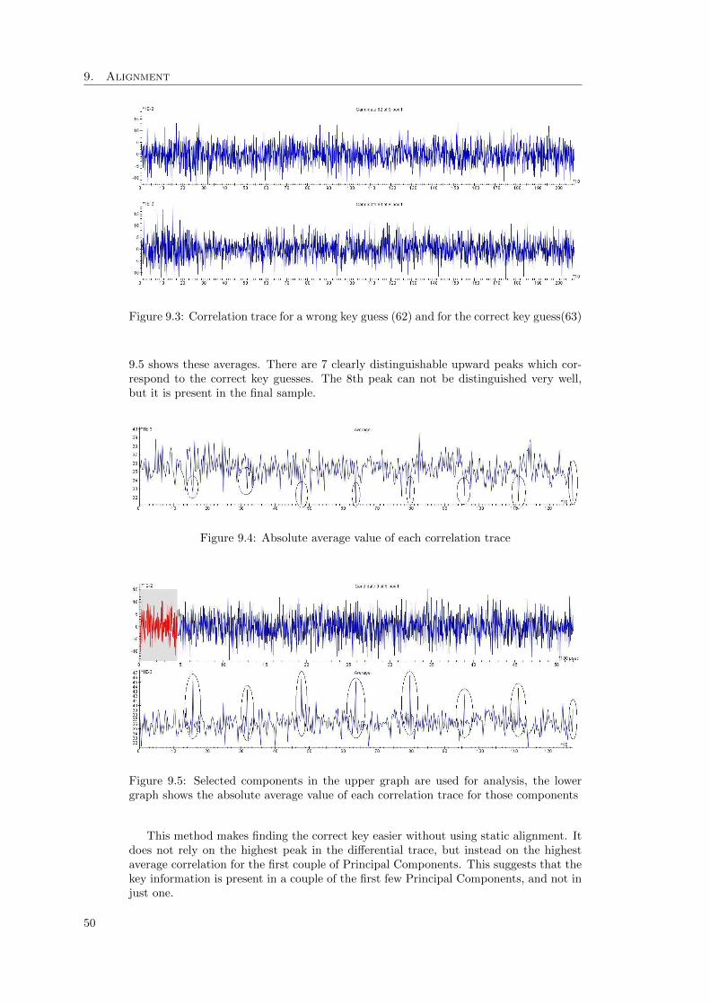
9. Alignment
Figure 9.3: Correlation trace for a wrong key guess (62) and for the correct key guess(63)
9.5 shows these averages. There are 7 clearly distinguishable upward peaks which cor-respond to the correct key guesses. The 8th peak can not be distinguished very well,but it is present in the final sample.
Figure 9.4: Absolute average value of each correlation trace
Figure 9.5: Selected components in the upper graph are used for analysis, the lowergraph shows the absolute average value of each correlation trace for those components
This method makes finding the correct key easier without using static alignment. Itdoes not rely on the highest peak in the differential trace, but instead on the highestaverage correlation for the first couple of Principal Components. This suggests that thekey information is present in a couple of the first few Principal Components, and not injust one.
50

9.2. PCA and Misalignment - Experiments
Table 9.1: Comparison between Static alignment and PCA
Static alignment Principal Com-ponent Analysis(first 100)
Principal Com-ponent Analysis(first 150)
Correct key guess 0.4035 0.0416 0.0450First wrong keyguess
0.2869 0.0405 0.0393
Difference betweencorrect and wrongkey guess (%)
28,2 2,6 12,7
9.2.2 A comparison between PCA and static alignment
The traces which were used in the previous chapters were all statically aligned in orderto make a DPA attack successful with a relatively small amount of traces. In the pre-vious experiment, we did not perform this alignment, but instead used PCA to capturethe samples with the same variance in the same component. Using this method, we werealso able to find the correct key, although not by finding the correlation trace with thehighest peak, but instead the correlation trace which had the largest absolute averagevalue for the first 70 components.
Since these two methods are totally different, we wanted to see how PCA comparesto static alignment. We compare these two methods by the height of the peak for thecorrect key guess. For static alignment, we look at difference in the height of the peakfor the correct key guess as opposed to the one for the first wrong key guess. For PCA,we look at the difference in the height of the average value of the correlation trace forthe correct key guess as opposed to the one for the wrong key guess.
For the values for static alignment, we use the misaligned traceset from sample card2 and statically align them before doing a DPA attack. For the values for PCA, weuse the misaligned traceset, perform a PCA transformation, and calculate the absoluteaverage value for 100 and 150 samples of the correlation traces. The results can be foundin table 9.1.
We can conclude from these results that if static alignment is possible on a traceset,it yields better results in that the correct key guess differs more from the first wrongkey guess. If static alignment is not possible for some reason, one can find the correctkey by using our method.
The main drawback of PCA is that there is a maximum to the number of sampleswe can use for our calculations. Remember that the correlation matrix of n ∗ n has tobe computed. Static alignment does not have this problem. If a traceset has a largesample size, static alignment would be preferred.
9.2.3 Random delays
In order to see if the method shown before also works with traces which are moremisaligned than only a couple of samples, we create power measurements of a DESencryption on sample card 2 with random delays as a countermeasure. This counter-measure introduces random delays within the execution of the DES algorithm. It usesDES to derive random numbers which are used as a seed for the delays. This causesmisalignment since the S-boxes are now processed in different samples which lie moreapart than in the misaligned traces we have seen before.
51
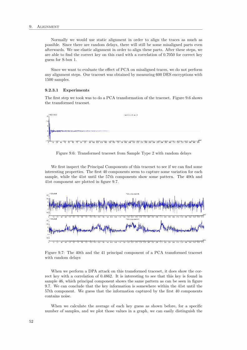
9. Alignment
Normally we would use static alignment in order to align the traces as much aspossible. Since there are random delays, there will still be some misaligned parts evenafterwards. We use elastic alignment in order to align these parts. After these steps, weare able to find the correct key on this card with a correlation of 0.7050 for correct keyguess for S-box 1.
Since we want to evaluate the effect of PCA on misaligned traces, we do not performany alignment steps. Our traceset was obtained by measuring 600 DES encryptions with1500 samples.
9.2.3.1 Experiments
The first step we took was to do a PCA transformation of the traceset. Figure 9.6 showsthe transformed traceset.
Figure 9.6: Transformed traceset from Sample Type 2 with random delays
We first inspect the Principal Components of this traceset to see if we can find someinteresting properties. The first 40 components seem to capture some variation for eachsample, while the 41st until the 57th components show some pattern. The 40th and41st component are plotted in figure 9.7.
Figure 9.7: The 40th and the 41 principal component of a PCA transformed tracesetwith random delays
When we perform a DPA attack on this transformed traceset, it does show the cor-rect key with a correlation of 0.4862. It is interesting to see that this key is found insample 46, which principal component shows the same pattern as can be seen in figure9.7. We can conclude that the key information is somewhere within the 41st until the57th component. We guess that the information captured by the first 40 componentscontains noise.
When we calculate the average of each key guess as shown before, for a specificnumber of samples, and we plot those values in a graph, we can easily distinguish the
52
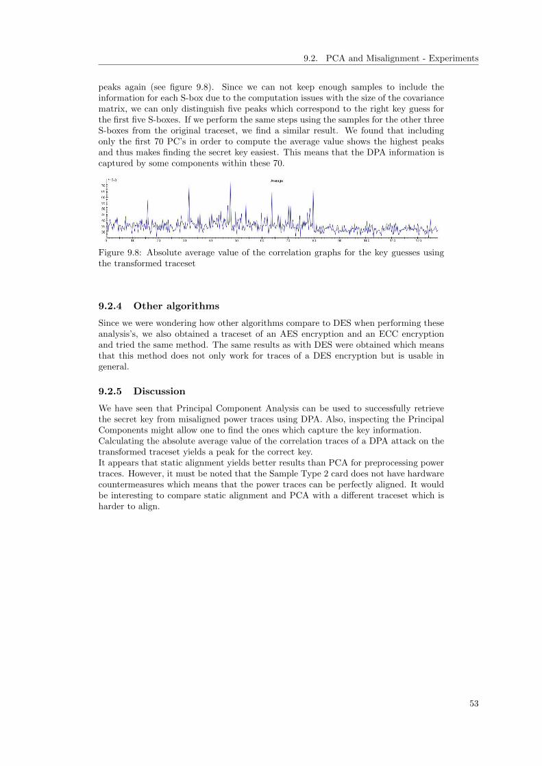
9.2. PCA and Misalignment - Experiments
peaks again (see figure 9.8). Since we can not keep enough samples to include theinformation for each S-box due to the computation issues with the size of the covariancematrix, we can only distinguish five peaks which correspond to the right key guess forthe first five S-boxes. If we perform the same steps using the samples for the other threeS-boxes from the original traceset, we find a similar result. We found that includingonly the first 70 PC’s in order to compute the average value shows the highest peaksand thus makes finding the secret key easiest. This means that the DPA information iscaptured by some components within these 70.
Figure 9.8: Absolute average value of the correlation graphs for the key guesses usingthe transformed traceset
9.2.4 Other algorithms
Since we were wondering how other algorithms compare to DES when performing theseanalysis’s, we also obtained a traceset of an AES encryption and an ECC encryptionand tried the same method. The same results as with DES were obtained which meansthat this method does not only work for traces of a DES encryption but is usable ingeneral.
9.2.5 Discussion
We have seen that Principal Component Analysis can be used to successfully retrievethe secret key from misaligned power traces using DPA. Also, inspecting the PrincipalComponents might allow one to find the ones which capture the key information.Calculating the absolute average value of the correlation traces of a DPA attack on thetransformed traceset yields a peak for the correct key.It appears that static alignment yields better results than PCA for preprocessing powertraces. However, it must be noted that the Sample Type 2 card does not have hardwarecountermeasures which means that the power traces can be perfectly aligned. It wouldbe interesting to compare static alignment and PCA with a different traceset which isharder to align.
53


Chapter 10
Conclusion
55

10. Conclusion
10.1 Conclusion
Differential Power Analysis is a widely used side-channel attack to find the secret keyused by a cryptographic device. By creating power measurements of a cryptographicencryption using a known plaintext, one can derive which secret key must have beenused using statistical methods.
We introduce Principal Component Analysis as a suitable preprocessing technique onthe power traces to enhance the results of Differential Power Analysis attacks. The twouses of PCA, noise reduction and a PCA transformation, were analysed for their effecton DPA attacks using different power measurements. In order to see what effect PCAhas on power measurements without any noise, we did some experiments on simulatedtraces. Since we also wanted to do some experiments on real-life traces, we obtainedpower traces from a smartcard with a software DES implementation, a smartcard witha hardware DES implementation and a SASEBO-R with an AES implementation.
Our experiments have shown that we were able to improve the signal to noise ratioin various occasions when the location of the key leakage is known. We were able toreduce the noise of a given traceset by retaining only the Principal Components whichcapture the variance at the location of the key leakage. The effect of this noise reductionwas that the guessed, correct, subkeys had a higher correlation when a DPA attack wasperformed on the noise-reduced traceset as opposed to the correlation on the originaltraceset. This method works for each of the tracesets we used.
We tried to find a threshold to decide which components can best be kept, andwhich components should be removed when performing a noise reduction using PCA.Components which had a variance above this threshold for the sample where the keyleakage is, were retained. Our experiments showed that there was no ’magic’ value forthis threshold.
Using PCA as a transformation in particular seems to show some interesting results.In our experiments, we transformed a traceset using PCA. On this transformed trace-set, we perform a DPA attack. In most cases, this did not yield the correct key. Wenoticed a visual difference in the correlation traces for the correct subkey and the wrongsubkeys. We introduced a method to find this difference in the correlation traces. Aftera DPA attack on the transformed traces, we calculate the absolute average value for allcorrelation traces for each subkey for a given number of components. We found that,in most cases, if we do this for the right number of Principal Components, which wefound by trial and error, the absolute average value for the correct key guess was higherthan for the other key guesses and thus showed a peak. The traceset for the SampleType 2 card showed a different behaviour than the other tracesets, we could not find anyupward peaks. Calculating the absolute average for the smallest components did showdownward peaks, which means that the correlation for these samples for the correct keyguess is much smaller than for the other, wrong, key guesses.
In order to perform an optimal DPA attack, power traces need to be aligned. Sincethe relation between the same samples of different traces is used, these samples needto be the result of the same operation. Manufacturers and researchers are constantlyresearching and implementing new countermeasures against side-channel attacks. Wehave found that PCA can be used to derive the secret key even in the presence of one ofthese countermeasures, the use of random delays. During the execution of the algorithm,a random amount of delays are introduced. These delays are used to make alignment ofthe power traces harder.Since Principal Component Analysis looks at the variance within a traceset instead ofa specific moment in time, introducing random delays has less effect. This means that
56
10.2. Further research
when we transform the original dataset using PCA, the samples with the same amountof variance are all captured by the same Principal Component. Experiments showedthat a DPA attack does not yield the highest peak for the correct subkey on this trans-formed traceset.The correlation traces which were obtained from the DPA attack did show some visualdifferences for the correct subkey as compared to the traces for the wrong subkey. Itwas found that the key information is captured by a couple of Principal Componentsinstead of just one as in a normal DPA attack. This means that the correlation also ishigh for a couple of Principal Components. We used our absolute average method tofind the peak for the correct subkey.
Since static alignment and PCA are both able to process misaligned power traces soa DPA attack is successful, we compared them. Performing DPA after a static align-ment showed a bigger difference between the correct and the first wrong key. It mustbe noted that we compared these methods on a traceset from a device without anyhardware countermeasures which makes a perfect alignment possible.
The main drawback of PCA is that one has to work with a relatively small samplesize. Since we need to calculate the n ∗ n-covariance matrix, increasing the number ofsamples causes the calculation time to increase quadratically. Our applet was able todeal with 2500 samples before running out of memory. In real-life situations, this mightnot be enough.
Our experiments were focussed on DES, but we obtained similar results when at-tacking AES, as we did with the SASEBO measurements, or ECC.
We conclude that using Principal Component Analysis to preprocess power traceshas a positive effect on finding the correct key using DPA attacks.
10.2 Further research
Although researching Principal Component Analysis answered some interesting ques-tions, diving into it also raised more questions. In this section we mention topics forpossible future research.
Our experiments only included tracesets with a small amount of samples due tocomputation issues. In real life, these tracesets can contain millions of samples and/ortraces. Also, we might not know the location of the key leakage. How can we applyPCA there?
We compared PCA with static alignment for a traceset taken from the Sample Type2 card. This card has no hardware countermeasures which makes it possible to do aperfect alignment. How does PCA compare with static alignment on a better protecteddevice?
We introduced a new distinguisher to find a peak for the correct key. We performeda PCA transformation on a traceset. Then we did a DPA attack. We took the absoluteaverage value for each resulting correlation trace. Using different parts of these correla-tion traces for this calculation showed different results. Further research could be intothe theory of this method.
57


Bibliography
[AO] Manfred Aigner and Elisabeth Oswald. Power analysis tutorial. Technicalreport, Institute for Applied Information Processing and Communication,University of Technology Graz.
[APSQ06] C. Archambeau, E. Peeters, F.-X. Standaert, and J.-J. Quisquater. Templateattacks in principal subspaces. In Cryptographic Hardware and EmbeddedSystems - CHES 2006, volume 4249/2006 of Lecture Notes in ComputerScience, pages 1–14. Springer Berlin / Heidelberg, 2006.
[AR03] J.R. Agrawal, D. Rao and P. Rohatgi. Multi-channel attacks. Lecture notesin computer science, 2779:2–16, 2003.
[AW10] Herv Abdi and Lynne J. Williams. Principal component analysis. Technicalreport, University of Texas at Dallas and University of Toronto Scarborough,2010.
[Bar08] William C. Barker. Recommendation for the triple data encryption algorithm(TDEA) block cipher. http://csrc.nist.gov/publications/nistpubs/
800-67/SP800-67.pdf, May 2008.
[BCO04] E. Brier, C. Clavier, and F. Olivier. Correlation power analysis with a leak-age model. Cryptographic Hardware and Embedded Systems CHES 2004,3156:16–29, 2004.
[BDL97] Dan Boneh, Richard A. DeMillo, and Richard J. Lipton. On the impor-tance of checking cryptographic protocols for faults. In EUROCRYPT’97:Proceedings of the 16th annual international conference on Theory and ap-plication of cryptographic techniques, pages 37–51, Berlin, Heidelberg, 1997.Springer-Verlag.
[BGLR09] Lejla Batina, Benedikt Gierlichs, and Kerstin Lemke-Rust. Differential clus-ter analysis. In CHES ’09: Proceedings of the 11th International Workshopon Cryptographic Hardware and Embedded Systems, pages 112–127, Berlin,Heidelberg, 2009. Springer-Verlag.
[BNSQ03] Lilian Bohy, Michael Neve, David Samyde, and Jean-Jacques Quisquater.Principal and independent component analysis for crypto-systems with hard-ware unmasked units. In In Proceedings of e-Smart 2003, 2003.
[Bri91] R. Briol. Emanation: How to keep your data confidential. Symposium onElectromagnetic Security For Information Protection (SEPI’91), November1991.
[BS93] Eli Biham and Adi Shamir. Differential cryptanalysis of the full 16-roundDES. In CRYPTO ’92: Proceedings of the 12th Annual InternationalCryptology Conference on Advances in Cryptology, pages 487–496. Springer-Verlag, 1993.
59

Bibliography
[Cat66] Raymond B. Cattell. The scree test for the number of factors. MultivariateBehavioral Research, 1:245–276, 1966.
[CRR03] Suresh Chari, Josyula R. Rao, and Pankaj Rohatgi. Template attacks. InCHES ’02: Revised Papers from the 4th International Workshop on Crypto-graphic Hardware and Embedded Systems, pages 13–28, London, UK, 2003.Springer-Verlag.
[Hot33] Harold Hotelling. Analysis of a complex of statistical variables into principalcomponents. The Journal of Educational Psychology, pages 417–441, 1933.
[HSH+09] J. Alex Halderman, Seth D. Schoen, Nadia Heninger, William Clarkson,William Paul, Joseph A. Calandrino, Ariel J. Feldman, Jacob Appelbaum,and Edward W. Felten. Lest we remember: cold-boot attacks on encryptionkeys. Commun. ACM, 52(5):91–98, 2009.
[Jol72] I.T. Joliffe. Discarding variables in a principal component analysis 1: Arti-ficial data. Applied statistics, 21:160–173, 1972.
[Jol02] I.T. Jolliffe. Principal Component Analysis. Springer Series in Statistics.Springer New York, second edition edition, 2002.
[KJJ99] Paul C. Kocher, Joshua Jaffe, and Benjamin Jun. Differential power analysis.In CRYPTO ’99: Proceedings of the 19th Annual International CryptologyConference on Advances in Cryptology, pages 388–397, London, UK, 1999.Springer-Verlag.
[Koc96] Paul C. Kocher. Timing attacks on implementations of diffie-hellman, RSA,DSS, and other systems. In CRYPTO ’96: Proceedings of the 16th AnnualInternational Cryptology Conference on Advances in Cryptology, pages 104–113, London, UK, 1996. Springer-Verlag.
[Man04] Stefan Mangard. Hardware countermeasures against DPA A statistical anal-ysis of their effectiveness. In Topics in Cryptology - CT-RSA 2004, TheCryptographers Track at the RSA Conference 2004, pages 222–235. Springer,2004.
[Mat94] Mitsuru Matsui. Linear cryptanalysis method for DES cipher. In EURO-CRYPT ’93: Workshop on the theory and application of cryptographic tech-niques on Advances in cryptology, pages 386–397. Springer-Verlag New York,Inc., 1994.
[MBB08] Abhilash Alexander Miranda, Yann-Ael Borgne, and Gianluca Bontempi.New routes from minimal approximation error to principal components. Neu-ral Process. Lett., 27(3):197–207, 2008.
[Mes00] Thomas S. Messerges. Power analysis attacks and countermeasures for cryp-tographic algorithms. PhD thesis, University of Illinois at Chicago, Chicago,IL, USA, 2000.
[MOP07] Stefan Mangard, Elisabeth Oswald, and Thomas Popp. Power Analysis At-tacks: Revealing the Secrets of Smart Cards (Advances in Information Secu-rity). Springer-Verlag New York, Inc., Secaucus, NJ, USA, 2007.
[MSS09] Amir Moradi, Mohammad Taghi Manzuri Shalmani, and Mahmoud Salma-sizadeh. Dual-rail transition logic: A logic style for counteracting poweranalysis attacks. Comput. Electr. Eng., 35(2):359–369, 2009.
[MVO96] Alfred J. Menezes, Scott A. Vanstone, and Paul C. Van Oorschot. Handbookof Applied Cryptography. CRC Press, Inc., Boca Raton, FL, USA, 1996.
60
Bibliography
[Nag75] L.W. Nagel. SPICE2: A computer program to simulate semiconductor cir-cuits. Technical report, Electronics Research Laboratory, University of Cal-ifornia, Berkeley, USA, 1975.
[Pea01] Karl Pearson. On lines and planes of closest fit to systems of points in space.Philosophical Magazine Series 6, 2:559–572, 1901.
[PM05] T. Popp and S. Mangard. Masked dual-rail pre-charge logic: DPA-resistancewithout routing constraints. Proc. 7th International Workshop CryptographicHardware and Embedded Systems (CHES 05), pages 172–186, 2005.
[PMO07] Thomas Popp, Stefan Mangard, and Elisabeth Oswald. Power analysis at-tacks and countermeasures. IEEE Design and Test of Computers, 24:535–543, 2007.
[QS01] Jean-Jacques Quisquater and David Samyde. Electromagnetic analysis(EMA): Measures and counter-measures for smart cards. In E-SMART ’01:Proceedings of the International Conference on Research in Smart Cards,pages 200–210, London, UK, 2001. Springer-Verlag.
[Res08] Research Center for Information Security, National Institute ofAdvanced Industrial Science and Technology. Side-channel At-tack Standard Evaluation Board, SASEBO-R, Specification, 2008.http://www.rcis.aist.go.jp/files/special/SASEBO/SASEBO-R-ja/
SASEBO-R_Spec_Ver1.0_English.pdf.
[RO04] Christian Rechberger and Elisabeth Oswald. Practical template attacks. InInformation Security Applications, 5th International Workshop, WISA 2004,Jeju Island, Korea, August 23-25, 2004, Revised Selected Papers, volume3325 of Lecture Notes in Computer Science, pages 443–457. Springer, 2004.
[Smi02] Lindsay I. Smith. A tutorial on principal components analysis.http://www.cs.otago.ac.nz/cosc453/student_tutorials/principal_
components.pdf, February 2002.
[SSI04] Daisuke Suzuki, Minoru Saeki, and Tetsuya Ichikawa. Random switchinglogic: A countermeasure against DPA based on transition probability. Tech-nical report, Mitsubishi Electric Corporation, Information Technology R&DCenter, 2004.
[ST04] Adi Shamir and Eran Tromer. Acoustic cryptanalysis: on nosy people andnoisy machines. Presented at the Eurocrypt 2004 rump session, 2004. http://people.csail.mit.edu/tromer/acoustic/.
[TAV02] Kris Tiri, Moonmoon Akmal, and Ingrid Verbauwhede. A dynamic and differ-ential CMOS logic with signal independent power consumption to withstanddifferential power analysis on smart cards. ESSCIRC 2002, pages 403–406,2002.
[TV04] Kris Tiri and Ingrid Verbauwhede. A logic level design methodology for asecure DPA resistant ASIC or FPGA implementation. In DATE ’04: Pro-ceedings of the conference on Design, automation and test in Europe, page10246, Washington, DC, USA, 2004. IEEE Computer Society.
[TV05] Kris Tiri and Ingrid Verbauwhede. Simulation models for side-channel infor-mation leaks. In DAC ’05: Proceedings of the 42nd annual Design Automa-tion Conference, pages 228–233, New York, NY, USA, 2005. ACM.
[US 99] US National Institute of Standards and Technology. Federal InformationProcessing Standard 46-3, Data Encryption Standard, 1999. http://csrc.
nist.gov/publications/fips/fips46-3/fips46-3.pdf.
61

[vWWB] J. van Woudenberg, M. Witteman, and B. Bakker. Improving differentialpower analysis by elastic alignment. http://www.riscure.com/fileadmin/images/Docs/elastic_paper.pdf.
[Wie94] Michael J. Wiener. Efficient DES key search. Technical report, School ofComputer Science, Carleton University, 1994.
[ZHT04] Hui Zou, Trevor Hastie, and Robert Tibshirani. Sparse principal componentanalysis. Journal of Computational and Graphical Statistics, 15(2):265–286,2004.

Appendices
63


Appendix A. PCAFilter source code
package sandbox.jip;
/**
* Copyright (c) 2010 Riscure BV. All rights reserved.
* @author Jip Hogenboom <[email protected]>
* Based on PCATemplateAnalysis by Jasper Van Woudenberg
*/
import java.util.ArrayList;
import java.util.Arrays;
import java.util.Collection;
import java.util.Collections;
import java.util.List;
import java.util.Vector;
import java.awt.Dimension;
import javax.swing.ButtonGroup;
import javax.swing.JCheckBox;
import javax.swing.JPanel;
import javax.swing.JLabel;
import javax.swing.JRadioButton;
import javax.swing.JTextField;
import java.awt.BorderLayout;
import javax.swing.border.TitledBorder;
import sandbox.jasper.lib.IncrementalStatistics;
import Jama.EigenvalueDecomposition;
import Jama.Matrix;
import com.riscure.signalanalysis.Data;
import com.riscure.signalanalysis.Module;
import com.riscure.signalanalysis.Trace;
import com.riscure.signalanalysis.TraceSet;
@SuppressWarnings("serial")
public class PCAFilter extends Module {
private IncrementalStatistics[] targetMean;
private Matrix pcaVectors[];
private Vector<Trace> resultTraces;
private Matrix[] pcaCovInverse;
private double[] pcaCovDet;
private double[][] initialtraces;
private Matrix covMatrix[];
private Matrix testMatrix;
private double[] stdVector;
private byte[][] data;
private JTextField keepSmallTextField;
private JTextField keepLargeTextField;
private JTextField keepSpecificTextField;
private JTextField removeSmallTextField;
private JTextField removeLargeTextField;
private JCheckBox noiseSuppressionCheckBox;
private JCheckBox transformationCheckBox;
private boolean noiseSuppression = true;

private boolean transformation = false;
private String title = "";
int KEEPSMALL = 0;
int REMOVESMALL = 0;
int KEEPLARGE = 0;
int REMOVELARGE = 0;
int KEEPSPECIFIC = 0;
boolean NOISESUPPRESSION = true;
boolean TRANSFORMATION = false;
/** init module */
public void initModule() {
prefix = "PCA filter";
moduleDescription = "Perform Principal Component analysis on a traceset
for noise reduction or a transformation";
moduleVersion = "1.0";
titleSpace = 128;
}
public JPanel initDialog() {
noiseSuppressionCheckBox = new JCheckBox("Noise Reduction", noiseSuppression);
transformationCheckBox = new JCheckBox("Transformation", transformation);
JLabel keepSmallLabel = new JLabel(" Keep small PC’s:");
keepSmallTextField = new JTextField("0");
keepSmallTextField.setPreferredSize(new Dimension(30, 26));
JLabel keepSpecificLabel = new JLabel(" Keep only a specific sample with
threshold 0.1 in the PC’s");
keepSpecificTextField = new JTextField("-1");
keepSpecificTextField.setPreferredSize(new Dimension(100, 26));
JLabel keepLargeLabel = new JLabel(" Keep large PC’s:");
keepLargeTextField = new JTextField("0");
keepLargeTextField.setPreferredSize(new Dimension(30, 26));
JLabel removeSmallLabel = new JLabel(" Remove small PC’s:");
removeSmallTextField = new JTextField("0");
removeSmallTextField.setPreferredSize(new Dimension(30, 26));
JLabel removeLargeLabel = new JLabel(" Remove large PC’s:");
removeLargeTextField = new JTextField("0");
removeLargeTextField.setPreferredSize(new Dimension(30, 26));
JPanel centerPanel = new JPanel();
centerPanel.setBorder(new TitledBorder("Simulation options"));
centerPanel.add(removeLargeLabel);
centerPanel.add(removeLargeTextField);
centerPanel.add(removeSmallLabel);
centerPanel.add(removeSmallTextField);
centerPanel.add(keepLargeLabel);
centerPanel.add(keepLargeTextField);
centerPanel.add(keepSmallLabel);
centerPanel.add(keepSmallTextField);
centerPanel.add(keepSpecificLabel);
centerPanel.add(keepSpecificTextField);
centerPanel.add(noiseSuppressionCheckBox);
centerPanel.add(transformationCheckBox);
return centerPanel;
}
public boolean initProcess() {
if (!super.initProcess())
return false;
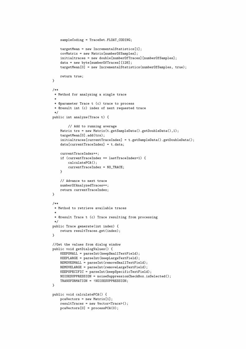
sampleCoding = TraceSet.FLOAT_CODING;
targetMean = new IncrementalStatistics[1];
covMatrix = new Matrix[numberOfSamples];
initialtraces = new double[numberOfTraces][numberOfSamples];
data = new byte[numberOfTraces][128];
targetMean[0] = new IncrementalStatistics(numberOfSamples, true);
return true;
}
/**
* Method for analyzing a single trace
*
* @parameter Trace t (c) trace to process
* @result int (c) index of next requested trace
*/
public int analyze(Trace t) {
// Add to running average
Matrix trs = new Matrix(t.getSampleData().getDoubleData(),1);
targetMean[0].add(trs);
initialtraces[currentTraceIndex] = t.getSampleData().getDoubleData();
data[currentTraceIndex] = t.data;
currentTraceIndex++;
if (currentTraceIndex == lastTraceIndex+1) {
calculatePCA();
currentTraceIndex = NO_TRACE;
}
// Advance to next trace
numberOfAnalyzedTraces++;
return currentTraceIndex;
}
/**
* Method to retrieve available traces
*
* @result Trace t (c) Trace resulting from processing
*/
public Trace generate(int index) {
return resultTraces.get(index);
}
//Get the values from dialog window
public void getDialogValues() {
KEEPSMALL = parseInt(keepSmallTextField);
KEEPLARGE = parseInt(keepLargeTextField);
REMOVESMALL = parseInt(removeSmallTextField);
REMOVELARGE = parseInt(removeLargeTextField);
KEEPSPECIFIC = parseInt(keepSpecificTextField);
NOISESUPPRESSION = noiseSuppressionCheckBox.isSelected();
TRANSFORMATION = !NOISESUPPRESSION;
}
public void calculatePCA() {
pcaVectors = new Matrix[1];
resultTraces = new Vector<Trace>();
pcaVectors[0] = processPCA(0);

numberOfResultTraces = resultTraces.size();
}
//Remove mean and divide by standard deviation if we do a noise reduction
//If we do a transformation, just remove the mean.
private Matrix centerMatrix(double[][] traces, IncrementalStatistics
targetMean, double[] stdVector, boolean noiseReduction) {
Matrix Mean = targetMean.getMean();
for(int i=0;i<numberOfTraces;i++) {
for(int j=0;j<numberOfSamples;j++) {
if(noiseReduction) {
traces[i][j] = ((traces[i][j] - Mean.get(0,j)) /
stdVector[j]);
} else {
traces[i][j] = ((traces[i][j] - Mean.get(0,j)));
}
}
}
return new Matrix(traces);
}
//multiply by standard deviation and add mean
private Matrix deCenterMatrix(double[][] traces, IncrementalStatistics
targetMean, double[] stdVector,
boolean removeZero, boolean noiseReduction) {
Matrix Mean = targetMean.getMean();
for(int i=0;i<numberOfTraces;i++) {
for(int j=0;j<traces[0].length;j++) {
//if value was removed, mean should not be added to prevent
weird calculations
if(traces[i][j] != 0 && !removeZero) {
if(noiseReduction) {
traces[i][j] = ((traces[i][j] * stdVector[j]) +
Mean.get(0,j));
} else {
traces[i][j] = ((traces[i][j]) + Mean.get(0,j));
}
}
}
}
return new Matrix(traces);
}
//Calculate the standard deviation
private double[] calcStd(Matrix Values, double[] MeanVector) {
//add all distances to mean, and divide by n-1
double[] totalPerColumn = new double[Values.getColumnDimension()];
for (int j=0;j<Values.getColumnDimension();j++) {
for(int i=0;i<Values.getRowDimension();i++) {
//std = sqrt((xi-x~)^2/n-1)
double a = ((Values.get(i,j) - MeanVector[j]) * (Values.get(i,j) -
MeanVector[j]));
totalPerColumn[j] += a;
}
totalPerColumn[j] /= Values.getRowDimension()-1;
totalPerColumn[j] = Math.sqrt(totalPerColumn[j]);
}
return totalPerColumn;
}

private Matrix createFeatureVector(Matrix V, int smallPCcutoff,
int largePCcutoff, double border,
int keeplargepc, int keepsmallpc,
int keepspecific) {
Matrix tmpMatrix =
new Matrix(V.getRowDimension(),V.getColumnDimension());
int numberOfPCs = 0;
//V: small PC -> large PC has to be flipped
if((largePCcutoff == 0) && (keepsmallpc != 0)) {
largePCcutoff = numberOfPCs - keepsmallpc;
}
if ((smallPCcutoff == 0) && (keeplargepc != 0)) {
smallPCcutoff = numberOfPCs - keeplargepc;
}
if(keeplargepc != 0 || keepsmallpc != 0) {
for (int i=V.getColumnDimension()-1;
i>V.getColumnDimension()-1-keeplargepc; i--) {
for(int row=0;row<V.getRowDimension();row++) {
tmpMatrix.set(row,V.getColumnDimension()-1-i,
V.get(row,i));
}
}
for(int i=0;i<keepsmallpc;i++) {
for (int row=0;row<V.getRowDimension();row++) {
tmpMatrix.set(row,V.getColumnDimension()-1-i,V.get(row,i));
}
}
} else {
for (int i=V.getColumnDimension()-largePCcutoff-1;
i>smallPCcutoff-1; i--) {
for(int row=0;row<V.getRowDimension();row++) {
if(((keepspecific == -1) ||
(Math.abs(V.get(keepspecific,i)) > 0.1))) {
tmpMatrix.set(
row,V.getColumnDimension()-1-i,
V.get(row,i)
);
if(row == 0) {
numberOfPCs++;
out(Integer.toString(
V.getColumnDimension()-i));
}
}
}
}
}
out("NUMBER OF PC’s USED: " + Integer.toString(numberOfPCs));
return tmpMatrix;
}
private Matrix processPCA(int t) {
// Get target mean
Matrix Tmean = targetMean[t].getMean();
testMatrix = new Matrix(initialtraces);
stdVector = calcStd(testMatrix,Tmean.getArray()[0]);
Matrix X = centerMatrix(initialtraces, targetMean[t],stdVector,NOISESUPPRESSION);

Matrix CovMatrix = targetMean[t].getCovariance();
EigenvalueDecomposition ed1 =
CovMatrix.times(numberOfTraces).
times((double)1/(numberOfTraces-1)).eig();
Matrix V = ed1.getV();
Matrix D = ed1.getD();
double cutoffValue = 0.00;
int removesmallpc = REMOVESMALL;
int removelargepc = REMOVELARGE;
int keeplargepc = KEEPLARGE;
int keepsmallpc = KEEPSMALL;
int keepspecific = KEEPSPECIFIC;
Matrix FeatureVector = createFeatureVector(
V,removesmallpc,
removelargepc, cutoffValue,
keeplargepc,keepsmallpc,
keepspecific
);
//W = V[]
//Y=X*U
Matrix FinalData = (X.times(FeatureVector));
Matrix origDeCenterMatrix = new Matrix(numberOfTraces,numberOfSamples);
if(NOISESUPPRESSION) {
//Z = U*(X*U)^T = U*U^T*X^T = X^T
Matrix RowDataAdjust2 = FeatureVector.times(FinalData.transpose());
//Z^T = X
origDeCenterMatrix = DeCenterMatrix(RowDataAdjust2.transpose().
getArray(), targetMean[t],
stdVector,false,NOISESUPPRESSION);
title = "Denoised trace ";
}
else if(TRANSFORMATION) {
origDeCenterMatrix = FinalData;
title = "Transformed trace ";
}
double [][] origarray = origDeCenterMatrix.getArray();
for(int i=0; i<origDeCenterMatrix.getRowDimension();i++) {
resultTraces.add(new Trace(title+i, data[i],
operation.createData(origarray[i])));
}
double[][] RowFeatureArray = V.transpose().getArray();
//Create plot for all Principal Components
for(int i=V.getColumnDimension()-1; i>-1;i--) {
double [] data = RowFeatureArray[i];
resultTraces.add(new Trace("PCA component "+
(V.getColumnDimension()-i), null, operation.createData(data)));
}

//Create plot of the eigenvalues
double[] vectors = new double[D.getColumnDimension()];
for(int i=D.getColumnDimension()-1;i>=0;i--) {
vectors[D.getColumnDimension()-1-i] = D.get(i,i);
}
resultTraces.add(new Trace("Eigenvalues ", null,
operation.createData(vectors)));
return V;
}
}