princeton the natural behavior available for everyone

The Natural Behavior of Unemployment

Robert Hall Markus BrunnermeierStanford Princeton

29. October 2020

Hosted from PRINCETONAvailable for EVERYONE,

WORLDWIDE

Webinar

1. When inflation is steady, neither rising nor falling over time, a) Unemployment is above its natural rateb) Unemployment is at its natural ratec) Unemployment is below its natural rate

2. The natural rate of unemploymenta) Is constant over time at around its long-term level of 5 percent.b) Has declined over time in recent decades, to 3.5 percent in February 2020,

before the pandemicc) Behaves according to stable principles, rising sharply in crises and declining

slowly during periods of economic calm.

3. High unemployment early in the pandemic (multiple choice)a) Completely departed from historical behavior--inflation remained stable at

close to 2 percent.b) Was consistent with historical behavior if workers who retain jobs but are on

temporary layoff are not considered to have a downward effect on inflation.c) Subsequently declined much faster than following other crises.

Bob Hall

Poll Results

Unemployment rate – policy dependency

USA Europe Breaks: job-worker matches maintain match: “Kurzarbeit”

Labor participation rate after GFC

German rise of socle/base unemployment

Economic miracle

Full employment

1st oil crisis

2nd oil crisis GFC Lehman

Labor market reforms

German unification

Unemployment rate Germany

Is there a NAIRU? Phillips curve

How is it connected to 𝑟𝑟∗?(Menger, Wicksell, Laubach-Williams)

How to 𝑢𝑢∗ ? Better matching technology Labor-search models?

(Davis-Haltiwanger, Shimer,…)

UnemplRate (BLS)

NAIRU (CBO)

Fed’s inclusion driveNo inflation explosion Greenspan inclusion drive Powell inclusion drive

New Fed policy framework Essentially eliminated NAIRU

NAIRU (CBO)

UnemplRate (BLS)

Greenspan Yellen/Powell

Thank [email protected]

The Natural Behavior of Unemployment

Robert E. Hall Marianna Kudlyak

Disclaimer: The opinions expressed are those of the authors and do not reflect those of the FederalReserve Bank of San Francisco, the Federal Reserve System, or the National Bureau of Economic

Research.

We thank Stephane Dupraz, Emi Nakamura, and Jon Steinsson for providing the code for their business-cyclechronology function and Marcelo Perlin for providing code for estimating hidden-Markov regime-switching models.

Milton Friedman, 1967, originates the natural rateof unemployment

The “natural rate of unemployment” ... is the level that would be ground out bythe Walrasian system of general equilibrium equations, provided there is imbeddedin them the actual structural characteristics of the labor and commodity markets,including market imperfections, stochastic variability in demands and supplies, thecost of gathering information about job vacancies and labor availabilities, the costsof mobility, and so on. (Friedman, 1967)

Nomenclature

We take the non-accelerating-inflation rate of unemployment (NAIRU) to be asynonym for the natural rate

In this paper

I We do not enter the thicket of general equilibrium models or empirical Phillipscurves.

I Rather, we study the behavior of unemployment in recoveries and document aregularity of the process.

I We believe that macro models should generate paths of unemployment withthese properties.

In this paper

The observed behavior of unemployment and thenatural behavior

Our empirical work is descriptive—it finds a parsimonious statistical description ofthe observed evolution of unemployment

After describing our approach and its findings, we return to the problem ofinferring the path of the natural rate from observed unemployment

The observed behavior of unemployment and thenatural behavior

Our empirical work is descriptive—it finds a parsimonious statistical description ofthe observed evolution of unemployment

After describing our approach and its findings, we return to the problem ofinferring the path of the natural rate from observed unemployment

Observed behavior of unemployment

We find that the observed behavior of unemployment comprises

I occasional sharp upward movements in economic crises

I at other times, an inexorable downward glide at a low but reliableproportional rate .

The glide continues until unemployment reaches approximately 3.5 percent or untilanother economic crisis interrupts the glide.

The paths of log-unemployment during recoveries

1949 1955 1961 1967 1973 1979 1985 1991 1997 2003 2009 2015

Our place in the literature

I Dupraz, Nakamura and Steinsson (2019) document the asymmetry of thebusiness cycle and cite a large earlier literature on that subject.

I We measure the rate of recovery of unemployment from recession-highs anddemonstrate how uniform the rate is.

I We develop a framework for inferring the natural rate from the observedbehavior of unemployment.

Recent influential papers with many references

Crump, Nekarda, and Petrosky-Nadeau (2020); Crump, Giannoni, Eusepi, andSahin (2019); Barnichon and Matthes, (2017); Coibion and Gorodnichenko (2015);Jorgensen and Lansing (2019); Hazell, Herreno, Nakamura and Steinsson (2020);Laubach (2001); and Staiger, Stock and Watson (1997)

Measurement

Measuring the business cycle

Two issues:1. What measure: output, unemployment, or latent “economic activity”?

2. Do we need to use a bandpass filter to remove a non-cyclical slower-movingtrend?

Following Romer & Romer (2019), we consider unemployment as an indicator littleaffected by forces other than the business cycle, so that choice of measure obviatesfiltering.

We consider the general class of statistical models

f(ut) = xt + εt,

where f(·) is a monotonic transformation, xt is the systematic trend componentcapturing the business cycle, and εt is the random unsystematic component, takento be uncorrelated with xt.

We pick the log transformation.

We use two econometric approaches:• a chronology-based approach• Hamilton’s (1989) Markov regime-switching model

f(ut) = xt + εt,

Chronology-based approach

Given a chronology, one can approximate the systematic component xt byinterpolating between the turning points and measuring the noise εt as the residualbetween log ut and xt.

The systematic trend component xt is a smooth function of t.

We take it to be a straight line between the turning points of the series, so xt hasequal increments over time, between the turning points.

Overall, the trend component is a linear spline.

Model for a single recovery

12(log uT − log u0) = −β T + εT − ε0

We include the 12 so that the recovery rate β of the recovery that starts in monthT (high point) and ends in month 0 (low point) is in log points per year.

We use the estimator

β = −12(log uT − log u0)

We use a quasi-bootstrap procedure to approximate the sampling distribution of β.

12(log uT − log u0) = −β T + εT − ε0

Available chronologies

1. NBER turning points in economic activity.

2. The output of a chronology-finding algorithm of Dupraz-Nakamura-Steinsson(DNS) applied to unemployment.

3. A chronology of the unemployment rate based on observed business cyclepeaks and troughs (HK).I Dates are similar to DNS; however, we pick the latest points for peaks and

troughs, consistently with our definition of the recovery.I Results are quite similar to DNS.

Results

Estimated Annual Log Unemployment RecoveryRate, Chronology-Based

NBERDupraz-Nakamura-Steinsson

Hall-Kudlyak

Full sample

Annual recovery rate, log points0.087 0.132 0.129

Standard error (0.016) (0.017) (0.017)

Standard deviation of recovery rate across recoveries 0.076 0.084 0.084Standard error (0.119) (0.117) (0.115)

After 1959

Annual recovery rate, log points 0.067 0.106 0.103Standard error (0.013) (0.007) (0.007)

Standard deviation of recovery rate across recoveries 0.025 0.011 0.016Standard error (0.038) (0.039) (0.038)

Chronology

Estimated Annual Log Unemployment RecoveryRate, by Recovery

1949 1954 1958 1961 1971 1975 1982 1992 2003 2009

Starting year

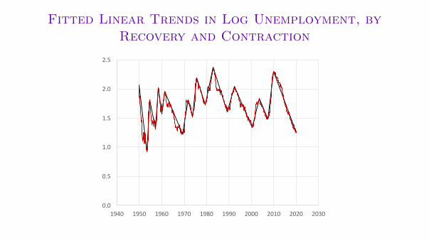
Fitted Linear Trends in Log Unemployment, byRecovery and Contraction

1940 1950 1960 1970 1980 1990 2000 2010 2020 2030

Estimated Annual Log Unemployment Recovery andContraction Rates, Hidden-Markov-Based

Full sample After 1959

Starting observation Oct-49 May-61

Ending observation Feb-20 Feb-20

Annual recovery rate, log points 0.066 0.070Standard error, quasi-bootstrap (0.042) (0.039)Standard error, information matrix (0.015) (0.014)

Annual contraction rate, log points 0.700 0.433Standard error, quasi-bootstrap (0.103) (0.051)Standard error, information matrix (0.078) (0.053)

Comparison of Chronology- andHidden-Markov-Based Log Unemployment Recovery

Rate Estimates

Full sample Later sample

Return rate, chronology based 0.132 0.106

Return rate, hidden-Markov based 0.066 0.070

Difference 0.066 0.036Quasi-bootstrap standard error of difference

(0.015) (0.012)

The key difference between the two approaches is the precision of information about

turning points. In the regime-switching model, turning points are latent unobserved events

and the model yields a probability that a given month is a turning point. Chronologies,

instead, treat turning points as unambiguous events.

Inferring the natural behavior of unemployment from theobserved behavior

Behavior of Unemployment vs a Constant NaturalRate

I We suggest that a notion of the natural behavior of unemployment shouldreplace the notion of a single natural rate fixed over time.

I The natural behavior of unemployment differs from the observed behavioraccording to principles similar to the literature on short-run deviations ofactual unemployment from the natural rate of unemployment.

Behavior of Unemployment vs a Constant NaturalRate

I We suggest that a notion of the natural behavior of unemployment shouldreplace the notion of a single natural rate fixed over time.

I The natural behavior of unemployment differs from the observed behavioraccording to principles similar to the literature on short-run deviations ofactual unemployment from the natural rate of unemployment.

Volatile Unemployment and Stable Inflation in thePast 30 Years

I Friedman’s analysis implies that years of stable inflation are years when theunemployment rate is at its natural level.

I High volatility of unemployment and highly stable inflation over the past 30years suggest that most of the movement in unemployment is movement of thenatural rate.

I So one idea would be to take actual unemployment rate as a goodapproximation to the natural rate.

Existing Approaches to Measuring the Natural Rateof Unemployment over Time

1. A longer-run average of the actual unemployment rate

2. A rate backed out of the Phillips curve

3. A solution from a model with nominal frictions removed

Our view on measurement

Methods 2 and 3 are likely to find large variations in the natural rate, trackingactual unemployment

That conclusion should be taken seriously

Our results suggest that all types of crises set a similar path of unemployment inmotion, once the initial impulse to unemployment occurs.

Conclusions

We have developed a parsimonious statistical model of the behavior of observedunemployment

It describes:(1) occasional sharp upward movements in unemployment in times of economiccrisis, and(2) an inexorable downward glide at a low but reliable proportional rate at allother times.

Conclusions

We have developed a parsimonious statistical model of the behavior of observedunemployment

It describes:(1) occasional sharp upward movements in unemployment in times of economiccrisis, and(2) an inexorable downward glide at a low but reliable proportional rate at allother times.

Conclusions (cont.)

The natural rate of unemployment derived from this model would bestate-dependent. It would be contingent on the severity of the most recent crisisshock and the number of months into the recovery.

In other words, the natural rate of unemployment in a given month is the averageover history conditional on the level at its most recent business-cycle high level andnumber of months that have elapsed from the trough to the given month.

We don’t yet have a position on the non-contingent natural rate

Conclusions (cont.)

As for policy,

The Fed’s new policy of not resisting the downward glide in unemployment duringperiods of calm is consistent with our conclusions.

Recovery from the 2020 Pandemic

The 2020 Pandemic Put Spotlight on the Unemployedwith and without Jobs

Both jobless-unemployment and recall-unemployment are associated with loweraggregate work effort and corresponding loss of earnings.

Jobless-unemployment follows the principles of modern search-and-matchingmodels, while workers suffering recall unemployment are waiting for recall.

The 2020 Pandemic Put Spotlight on the Unemployedwith and without Jobs

Both jobless-unemployment and recall-unemployment are associated with loweraggregate work effort and corresponding loss of earnings.

Jobless-unemployment follows the principles of modern search-and-matchingmodels, while workers suffering recall unemployment are waiting for recall.

Findings

• Prior to the pandemic, recall-unemployment was unimportant.

• The pandemic caused an explosion of recall unemployment.

• In the pandemic, recall-unemployment returned rapidly toward normal whilejobless-unemployment rose somewhat.

• We are monitoring the evolution of jobless-unemployment andrecall-unemployment to gauge the recovery.

Findings

Historical recall- and jobless-unemployment

1965 1970 1975 1980 1985 1990 1995 2000 2005 2010 2015 2020

Unemployment rate from temporary layoff, SA

Unemployment rate for reasons other than temporary layoff, SA

Pandemic recall- and jobless-unemployment

Jan‐19

Feb‐19

Mar‐19

Apr‐19

May‐19

Jun‐19

Jul‐1

Aug‐19

Sep‐19

Oct‐19

Nov‐19

Dec‐19

Jan‐20

Feb‐20

Mar‐20

Apr‐20

May‐20

Jun‐20

Jul‐2

Aug‐20

Sep‐20

Unemployment rate from temporary layoff, SAUnemployment rate for reasons other than temporary layoff, SA

princeton the natural behavior available for everyone

Documents