price responsiveness of world grain markets: the...
TRANSCRIPT

Ig 12~ ~~ 10 ~~ RfiI=I 0
IIIII~middot~ I~ 22 11111 ~ 136
I ut
f 1pound 0I I ~
IIIII~ ~~~ 1111118
11111 125 11111 1411111 16_
Price Responsiveness of World Grain Markets The Influence of Gevernment Intervention on Import Price Elasticity By Terry Roe Mathew Shane and De Huu Vo International Economics Division Economic Research Service US Department of Agriculture Technical Bulletin No 1720
Abstract
Intervention by governments in their foreign trade sectors fundamentally alters the character and composition of agricultural trade by making imports less responsive to international price changes than they otherwise would be Intervention can also make world market prices change more frequently and more drastically The authors developed a model of government intervention and applied it to the international wheat and rice markets using combined cross-country and time-series data Using an estimated import equatioll they measured the responsiveness of import demand and excess demand to price changes and the extent to which price changes are transmitted to final consumers Based on this study the authors concluded that governments reduced the degree of intervention between 1967 and 1980 and that US agriculture is in a good position to benefit from relaxed trade restrictions Also increased per capita income does not necessarily increase demand for imported goods rather increased per capita export revenues generate the basis for increased purchases of imports
Keywords Import elasticities government intervention international trade wheat and rice markets
Acknowledgments
This work is part of a broader study on growth market countries being undertaken by the Agricultural Development Branch Terry Roes participation was financed under a cooperative agreement between ERS and the University of Minnesota Lon Cesal provided considerable help and encouragement Phil Abbott Alex McCalla and Jim Houck in the profession and T Kelley White John Dunmore Nicole Ballenger Carlos Amade Chong Kim and Tom Vollrath in ERS provided valuable comments and suggestions Lindsay Mann provided valuable editorial assistance with the manuscript Charles Rodgers assisted in the study and Jamesena George typed the manuscript
Washington DC 20005-4788 June 1986
11
Contents
Page
Summary _ iv
Introduction
Prior Research in Import Elasticity 2
The Government Intervention Model 3
Empirical Model 7
Empirical Estimation of Wheat and Rice Imports 9
Elasticity Estimates Impiications of the Empirical Results 12
Conclusion 17
References 20
Appendix 1 The Derivation of the Import Demand Elasticity 22
Appendix 2 Definitions of Variables 24
Appendix 3 Country Data 26
Additional copies of this report
can be purchased from the Superintendent of Documents US Government Printing Office Washington DC 20402 Ask for Price Responsiveness of World Grain Markets The Illfluellc of Government Intervention on Import Price Elasticity (TB-1720) Write to the above addresses for price and ordering instructions For faster service call the GPO order desk at 202-783-3238 and charge your purchase to your VISA MasterCard Choice or GPO Deposit Account A 25-percent bulk discount is available on orders of 100 or more copies shipped to a single address Please add 25 percent extra for postage for shipments to foreign address
Microfiche copies ($595 each) can be purchased from the order desk National Technical Information Service 5285 Port Royal Road Springfield VA 22161 Ask for Price Responsivelless of World Grain Markets The Influence of Governmellt Interlelllioll Oil Imporl Price Elasticity (TB-1720) Enclose check or money order payable to NTIS For faster service call NTIS at 703-487-4650 and charge your purchase to your VISA MasterCard American Express or NTIS Deposit Account NTIS will ship rush orders within 24 hours for an extra $10 charge your rush order by calling 800-336-4700
The Economic Research Service has no copies for free mailing
111
Summary
Intervention by governments in their foreign trade sector fundamentally alters the character and composition of agricultural trade by making imports les~ responsive to international price changes than they otherwise would be Intervention can also make world market prices change more frequently and more drastically
The authors developed a model of government intervention and applied it to the international wheat and rice markets using combined cross-country and time-series data Using an estimated import equation they measured the responsiveness of import demand and excess demand to price changes and the extent to which price changes are transmitted to final consumers Based on this study the authors concluded that governments reduced the degree of intervention between 1967 and 1980 and that US agriculture is in a good position to benefit from relaxed trade restrictions The authors also concluded that increased per capita income does not necessarily increase demand for imported goods rather increased per capita export revenues generate the basis for increased purchases of imports
Other findings include the following
o Import decisions tend to be less responsive to price changes when a government intervenes strongly in the international market than when a government intervenes less or not at all
o From 1967-80 the governments of the study countries increasingly reduced their intervention in international markets for wheat and rice
o Government intervention has made world wheat and rice prices react more drastically to economic shocks such as oil embargoes
o Countries which have low per capita incomes and which rely significantly on imports for basic foodstuffs such as the African countries south of the Sahara are less likely to respond to price changes
a Wealthier countries such as the oil-exporting countries of North Africa and the Middle East have greater choices among food imports and respond more to prices when making import decisions
o Per capita income growth does not necessarily cause imports to grow Per capita export growth is more important because increased foreign exchange earnings permit increased commercial imports
iv
Price Responsiveness of World G rain Markets The Influence of Government Intervention on Import Price Elasticity
Terry Roe Mathew Shane De Huu Vo
Introduction
The issue of how foreign markets respond to price changes is critical in designing appropriate trade and agricultural policies If import demand is elastic then policies which raise US agricultural prices will significantly dampen imports in other countries if import demand is inelastic however imports will continue at comparable levels and US export revenue will rise as prices increase
To study this issue we developed the following objectives
To identify the specific import elasticities which might be affected by government intervention
To identify the types of government intervention which might affect import elasticities
To determine long-term trends in government intervention and assess their effects on world markets
To compare import elasticities under government intervention and under free market situations
We analyzed the effect of government intervention on import behavior using a formal model of endogenous government behavior By posing a government choice function and deriving the implied import demand function we moved away from the traditional excess demand approach We pooled both cross-section and time-series data to estimate this relationship because this data base gives us the single most consistent means for estimating the relationships we believed exist
We specified our empirical model in terms of exogenous shift variables which are proxies for political factors affecting alternative policies for many countries Although we readily admit that the selected variables imperfectly reflect the factors affecting government policies we could find no better available variables for a wide spectrum of countries
Our empirical analysis focused on 72 countries for the petiod 1967-80 We estimated import excess demand and price transmission elasticities for wheat and rice Of the 72 countries 70 imported wheat and 56 imported rice We excluded from our estimates countries with zero imports
Roe isa professor of agricultural and applied economics University of Minnesota Shane and Vo are economists with the International Economics Division Economic Research Service US Department of Agriculture
1
Prior Research in Import Elasticity
Traditional commodity models of foreign demand have typically taken a free market approach to the estimation of import elasticity Under this formulation (16 27 and others) the import elasticity (EIij) is the sum of domestic demand (EDij) and supply (ESi) elasticities weighted by Import shares (IDij= QDijlQIi and ISij = QSiQIi)lI When domestic and border prices are different import elasticity must -be further weighted by the price transmission elasticity (Epij)b In this case the import elasticity of demand can be expressed as
(10)
where (EDijIDij - ESijISij) is the excess demand elasticity
Assume for instance that the domestic demand elasticity (ED) is -02 that the domestic supply elasticity (ES) is 04 and that the import demand and supply shares (I and IS) areD11 and 10 respectively Then the excess demand elasticity of demand (EE) is -62 The influence of the price transmissions elasticity on the import demand elasticity can be great Now assume that the price transmission elasticity is only 02 The import demand elasticity then becomes -12 instead
Numerous governments intervene in their foreign trade markets A recent study of 21 developing countries found that 19 exercised direct control on imports or exports or both of cereals through a government export-import monopoly import licenses export taxes or quotas QQ) In economies with government intervention the domestic forces of supply and demand are not necessarily reflected in the countrys foreign trade behavior If governments intervene to attain specific economic objectives the excess demand elasticity can differ substantially from the import demand elasticity
The approach employed by Tweeten Johnson (2) and others to obtain import demand elasticities does not endogenize government intervention behavior Bredahl Meyers and Collins addressed that shortcoming when they concluded
In cases where governments insulate internal production and consumption from world markets the Ep [price transmission elasticity] will be at or near zero
However Bredahl Meyers and Collins do not incorporate a theory of government behavior Rather they posit a system in which the price transmission elasticity is zero or near zero if governments intervene and one otherwise
We developed a more direct means of creating an empirical basis for estimating import demand elasticity We maintain that governments intervene in their foreign trade sectors purposefully by choosing levels of policy instruments to affect consumer and producer welfare and the Treasury]j
Using an approach similar to that developed by Abbott 0 and expanded by Gerrard and Roe 01) Sarris and Freebairn ~ and Riethmuller and Roe we developed a method
1 For the derivation of this equation see appendix 1 The subscripts I D and S refer to import demand and supply and the ij subscript refers to the ihcommodity in the jcountry For the remainder of this report the ij subscript will often be assumed but for convenience not written (read Er E1ij) Also there is an implicit time sUbscript (t) associated with each variable Underlined numbers in parentheses identify literature cited in the references at the end of th~ report Jj Epij (apdijlapwij)(PwijPdj) where P dij is the domestic price of the ihcommodity in the jb
country and P w is the respective border price ~ In a multiperiod model a positive Treasury position can be viewed as a subsidy for consumers and producers in later
periods A single-period model assumes that these concerns are embodied in the utility the government obtains from the Treasurys position
2
for deriving import demand excess demand and price transmission functions from patterns of government behavior These functions form the basis for estimating elasticities as expressed in equation (10)
Fitting these functions to data for a lar3e number of countries involves some important decisions especially whether to use time-series cross-section or pooled data Which type of data is used will determine th~ appropriate definition of variables so that variations across countries reflect uniform respnses to change rather than changes in scale The empirical model must also be specified with fixed empirical parameters to allow for adjustment based on country-specific characteristics Individual estimates for each country would be ideal however sufficient data to estimate elasticities for a reasonably large set of individual countries are very limited With appropriate normalization of variables the pooling of cross-section and time-series data therefore provides the best overall consistent results across countries
We analyzed the effect of govemment intervention on import behavior using a formal model of endogenous government behavior By posing a government choice function and deriving the implied import demand function we moved away from the traditional excess demand approach We used pooled cross-section time-series data to estimate this relationship because we felt that these data gave us the single most consistent means for estimating the relationships we believed exist We specified our empirical model in terms of exogenous shift variables which are proxies for political factors affecting alternative policies for many countries Although we readily admit that the selected variables imperfectly reflect the factors (ffecting government policies we could find no better available variables for a wide spectrum of countries
The Government Intervention Model
Within a partial- quilibrium context a governments motivation for intervening in a particular market can be specified as a function of only two criteria
o the area under the excess demand function (A) representing the tradeoff of consumer and producer interests and
o the net revenue position of the government (NR) in marketing imports
We can also assume that the government exercises through whatever mechanism direct control over net trade (QI)~ This function (U) can be written as follows
(20) U= U(A NR Q(zraquo
where Q(z) denotes the parameters Q of U which are determined by unknown political variables We assumed the function U() to be a CQncave monotonically increasing function in both A and NR which is implied by the assumption of strict concavity in QI Here we maintain that the government chooses the level of its policy instrument net trade as though it sought to optimize (20) Implicitly we assumed the government knows the underlying supply and demand reiationship embodied in A
if There are of course numerous instruments which the government can control These include among other things domestic consumer and producer prices exchange rates taxes tariffs and subsidies of various kinds Moreover a government is almost surely concerned with economic activity in other sectors Howeverfrom the point of view of evaluating the import demand function those policies which isolate the domestic market from the world market are important The solution of the more general problem requires a general equilibrium statement of the problem which would unnecessarily distract from the focus of this report
3
If we assume no stockholdings and market clearance at a single price the quantity imported (QI) equals excess demand (QE)
(21)
where the two right-hand terms are domestic demand and supply as a funGtion of domestic price Pd Income and all other prices in the sense of partial equilibrium are treated as parameters Thus we can define the criteria of (20) as follows
(22) A = - PdQI + ofqpdCQI)dQI
(23) NR = PdQI - PwQI
where Pw is the border price and Pd(QI) is the excess demand function The governments problem is to find QI to maximize U
We assume that the ratio of marginal utility weights (8Uj8A)j(8UjBNA) equals one The first order necessary and sufficient condition characterizing a maximum of (20) in this case is 2
(112)
Thus when the ratio of the marginal utility weights is one the domestic and the border price are equal and the government may be said to be unbiased Hence our model does not by construction prevent a free-trade solution
Now suppose that the ratio of marginal utility weights is not one so that the government has a biased preference If we let Q = 8Uj8A andgt = 8Uj8NR then from the first order condition we obtain
(24)
Thus if Q is less than gt P d is greater than Pw the converse is true if Q is greater than A Using (24) the relative bias might be estimated by
(25)
Using the implicit function theorem we can determine the governments decision rule for imports (that is the import demand function) by solving (24) for QI Let
(30)
denote this result We can derive the inverse excess demand function from (21) and denote it as
(31 )
We then obtain the price transmission equation by substituting (31) into (25)
(32)
Y The maximization follows directly from use of the chain rule on (20) Thus
8u8Qr = (8U8A)(8A8Qr) + (8u8NR)(8NR8Qr)
Substituting in the partial derivations frotn (22) and (23) and assuming (8u8A)(8u8NR) equals one leads to the result
4
Equation (31) is independent of government preferences Clearly equations (30 31 and 32) are not independent of each other
Assuming linear functions we can diagram the import demand function on the price and import axis (fig 1)21 Note that a change in bias implies a rotation of the import demand function Because we are implicitly assuming a single market clearing domestic price the domestic excess demand function is identical to that of the free marketJl
A two-commodity model that does not distinguish among producers or among consumers of the two commodities but does distinguish between producers and consumers is a slight generalization of the previous model In this case the governments criterion function corresponding to (20) can be expressed as
(20)
The market-clearing consumer surplus and government expenditure equations are
(21 ) Qn = QEi == QDi(PdrPdw) - QSi(PdpPdw)
(22) Ac =Li(-PdiQn + oSqipdi(QlrQrw)dP di)
and
(23)
where the index i = rw denotes commodities rand w respectively Conditions (24) and (25) remain unchanged for each commodity The import demand function
(30)
where Pwr and Pww denote the border prices for rand w respectively follows from the implicit function theorem The inverse excess demand functions
(31 )
and the price transmission equations
(32)
are derived in a manner similar to (30) and (32)
sect In the case of linear supply and demand functions we can easily show that the import demand inverse excess demand and the price transmission equation can be expressed as
QI == ((gt(2gt-a))(a-bPw)
= (a-QE)b andP d
P d = (a-gt)ab+a + (gta)Pw
~spectively where a (whkh embodies other price and income effects) and b are parameters and 2gt-a =0 is assumed11 In more complex cases of government intervention the government uses producer and consumer prices as policy instruments
Under these cases the domestic excess demand function and the import demand function will shift with changing utility weights Note that we make a clear distinction between the import demand function which depends in general on import prices government utility weights and macroeconomic policy variables and the excess demand function which is primarily driven by domestic consumer and producer behavior through domestic prices The distinction between these functions has not been brought out in the literature Furthermore thio distinction clearly separates allocative intervention which distributes the benefits to different groups from scale intervention which separate the domestic and international markets For the problem of import demand scale intervention is more important The function U() contains the parameters Q(z) which over time may vary as a function of social and political factors (z)
5
Figure 1
Import Demand Function Under Government Intervention
PD Pw
PD(a)A) ~----------+-~-+----~
The import demand curve when the marginal utility of increasing A is greater than NR(a)A)
The import demand curve equals the domestic excess demand curve The government choice function is unbiased (a=A)
The import demand curve when the marginal utility of NR is greater than that of A(a(A)
Aamiddot2A-a (A) a)
Aamiddot2A-a (a)A)
The deviation of the import and excess demand and the price transmission elasticities for r ald w along he lines of (10) can be simply stated as
where it is easily shown that the right-hand term in brackets is equivalent to the first right-hand term in (10) If the price transmission elasticity is one then the import and excess demand elasticities are equal Hence as price transmission elasticity moves away from one government preferences ()a) will also vary from one (25) so that the free trade case (24) rannot occur In the case of linear demand and supply (see footnote 7) ) greater than a implies a transmission elasticity greater than one and vice versa
Empirical Model
To estimate our empirical model we could have applied our import demand model to a single country during a period over which the parameters Q(z) of (20) are constant However we generally would not expect these parameters to be constant across countries or through time Thus we specified the empirical model to accommodate parameters that are not constant by using pooled cross-section time-series data for 72 countries over 14 years Several researchers have used pooled cross-section time-series data to estimate econometric models (L l1lb 1Q) In our study we use this procedure to estimate global import demand elasticities which are a composite of individual country elasticities We included interaction variables designed to capture the unique contribution of each countrys economy to the global economy in the empirical model Thus the procedure generates both country-specific and global estimates of import elasticities However we will only discuss the estimates of global import elasticities A consideration of the statistical significance of individual country elasticities is beyond the scope of this report
With respect to specifying our empirical model the counterpart of the import demand and price transmission equations(30) and (32) are respectively
= eaoip alip a2ip a3ip a4ip a5ipXTa6ie (E30) ww wr wf wo wp I
(E32) = ecoip cliy i = r w WI l
where exponential terms are coefficients and ei and Yi are disturbance terms The variables pwf p wo P wp and PXT are the border prices of feedgrains oilseeds petroleum and per capita total exports respectively Because only two of the three equations embodied in (40) need to be estimated we chose (E30) and (E32) The price transmission relationship is straightforward and can be estimated directly from existing councry data Hence we omit the excess demand equations (31 ) and estimate their direct price elasticities as a residual from the other two directly estimated elasticities
Our elasticities are functions of both demand anj supply parameters and the government criterion function which is embodied in the (z) parameters Thus the estimated parameters generally reflect the combined effects of both as well as the interaction between them If the model is correctly specified the estimated parameters will reflect the expected economic relationships
The model specified for this study uses three factors to reflect differences between each countrys economy and the global economy These factors are reflected in the estimated coefficients aiO ail and ai2 One coefficient is an index of the real exchange rate (ERj) whIch measures the tendency for a countrys currency to be over- or undervalued reflectmg
7
the countrys pohey environment The second variable the relative net trade share (NRCAij)~ provides a measure of how important a commodity is to a countrys trade Finally the ratio of rice and wheat production to consumption (PCij) is a measure of the importance of trade in relation to domestic needs
To capture changes in parameters among countries and across time we define
aoi LhbohZh
ali LhblhZh
a2i Lhb2hZh
where (Z 1 Z2 Z4) - (1 NRCAi ER PCi) To keep our model simple and retain our focus we allowed for interaction terms only with the direct price effect and with the cross-price effect of rice in the wheat equation and vice versa In the case of the price transmission equations only the relativ9 trade shares (NRCA) exchange rate indexes (ER) and productionfood consumption ratio (PC) are employed as shifters Thus
In a framework of an import demand function with government intervention one would expect the availability of foreign exchange which we measure by total exports per capita (PXT) to provide the equivalent of an income constraint for import demand in contrast to an excess demand framework where demand is driven by prices and income Other exogenous variables that might affect the governments choice of imports of rice and wheat are border prices of food substitutes complements and petroleum price given its relatively large share of import expenditures in mal~y countries
We employed the small country assumption namely that the level of imports for the j country in the t- year has a negligible effect on world prices Although this assumption is reasonable for most countries in the sample it is quite unlikely in others To treat the probh~m otherwise however is to significantly compFcate the fitting of the model to available data
The conceptual framework assumes that governments choose the level of net imports QI in period t-l so that these quantities actualiy enter the market during period t We further assume that the government has perfect knowledge of the supply and demand conditions prevailing in the economy In reality a government probably would not have that knowledge Instead governments probably form expectations of the next periods demand and supply conditions However to incorporate an expectation formation mechanism for each country in the sample would quickly exhaust the degrees of freedom of the 14-year time series for each country Thus we continued to assume that governments have perfect foresight so that the independent variables specified in equations (E30) and (E32) can be treated as exogenous While the residual terms may still not be independently distributed no evidence of simultaneous equations bias was revealed in the empirjcal results
Ordinary least squares (OLS) estimation is unbiased in this case However the potential for significant heteroskedasticity exists We thus choose a generalized least square (GLS) procedure to account for country-to-country differences Country population over world population is used as a weighting factor The results exceeded our expectations for adherence to classical conditions even without imposing cross-equation restrictions
sect See appendix 2 for defini~ion
8
Our sample included 72 countries over the period 1967-80 70 countries import wheat and 56 import rice We excluded countries which do not import either wheat or rice
Three specific data problems must be dealt with to get meaningful results when estimating rarameters from a pooled data set
o Scale Without appropriate normalization some variables would represent scale factors rather than underlying economic relationships because countries differ dramatically in size The fact that Indias GNP is bigger than Jamaicas has very little economic significance for our analysis Scale problems were handled by defining scale variables in per capita terms
o Common units Many of the variables were initially defined in local currency units A systematic approach to converting these into common units was necessary and was particularly important because more than one method is available The most common technique is to convert the nominal local currency values into current US dollars through the current exchange rate However the new valu~ although in common units is now a function of both the original series and changes in exchange rates We converted each series into real valued local currency units first and then applied a fixed base year exchange rate Thus the variations now reflect the underlying changes in the base series and not in exchange rates Exchange rates can be brought in as a separate variable but they present particular problems for pooled data analysis To overcome these problems we converted the real exchange rates into an index with a common 1973 base year
o Real values We wanted our variables to reflect as much as possible real values rather than nominal values because our concern is with fundamental import behavior We converted the commodity production consumption and trade figures to wheat equivalent units using calorie conversions developed by the Food and Agriculture Organization of the United Nations We converted our macroeconomic variables gross national product (GNP) and total exports first into real local currency values through the use of GNP and export price deflators from the World Banks World Tables series and then converted that to constant 1973 US dollar through the use of the 1973 fixed exchange rate
Empirical Estimation of Wheat and Rice Imports
The results from applying our import demand function (E30) to data for rice and wheat appear in table 1 and table 2 The results closely adhere to prior conditions of import demand functions in spite of the fact that we did not impose such conditions on the system Moreover the sum of the mean own price (-050998) cross price (007094) and export elasticities (0435372) is almost zero in the wheat equation They are marginally negative in the rice equation The cross price elasticities of the two equations are surprisingly close to being equal (007094 and 0091884 bottom of tables 1 and 2) The most significant variable in the equations is per capita total exports A I-percent increase in per capita exports implies an approximate increase for both wheat and rice imports of almost 044 percent21
All coefficients associated with the rice and wheat import price variable are significant at the 99-percent level In the rice case only the base value of the import price elasticity is not significant The goodness-of-fit results measured by the adjusted R 2 at 087 and 083 are reasonably lar~ for pooled data results
E In our initial estimates we included per capita income as an independent variable along with price and per capita exports However per capita income never came into any estimating equation as a significant variable For the government import equation export earnings take the place of income in a domestic demand function
9
Table 1--Pooled data per capita wheat illlOrt demand equation
Inde~ndent variable Coefficient T-statistic Mean valle
Intercept Production-food consllllption shifter Wheat import price variable Base value Trade share shifter Exchange rate shifter Production-food consumption shifter
Rice illlOrt price cross variable Base value Trade share shifter Exchange rate shifter PIoduction-food consumption shifter
Feed grain import price oilseed illlOrt price International oil price Per capita total real exports
4_461324 6_1806 1 bull 097934 6 bull 0557 06719
1536104 3_4428 374m 6_1284 - 5137
- bull013254 -3 bull 0311 1015462 - _755431 -43596 6719
-1139350 -4_1806 - 398571 -7_3053 - 5137 bull010461 27158 1015462 488835 29643 6719
- 267497 -49297 158_110 - 241467 -47693 223_007
_002557 33578 86607 435372 16_7148 442 bull0603
-Adjusted R2 = 08685 -Number of observatio~s = 980 -Degrees of freedom = 964 -Standard error of the estimate = 24785 -Dependent variable = Per capita wheat import quantity -W(ighting factor = Country populationworld population -Form of the equation--Log-log with varying country parameters on wheat illlOrt price and rice import price
-Data coverage--70 countries 1967-80 -Direct price elasticity estimate at mean variable v~lues =-0_50998 -Cross price elasticity at mean variable value = 0 bull07094
-- =No value to specify_
Table 2--Pooled data per capita rice import demand equation
Independent variable Coeff i ci ent T-statistic Mean value
Intercept Production-food consumption shifter Rice import price variable Base value Trade share shifter Exchange rate shifter Production-food consumption shifter
Wheat import price cross variable Base value Trade share shifter Exchange rate shifter Production-food consumption shifter
Feed grain import price oilseed import price International oil price Per capita total real exports
5_364787 7_7011 -1_955932 -4_1147 08271
- bull041256 -_1174 -_117753 -4 8347 -1_1307 - _012365 -36938 102_9551
629491 57877 _8271
- 725832 -1_8743 070447 27888 -11307 011663 31510 1029551
- 366803 -3_6227 _8271 - 113700 -2_4451 162_9835 - _295057 -6_2329 2226139 bull004085 63319 8_6607 441707 14_4860 562_7990
-Adjusted R2 = 08259 -Number of observations = 784 -Degrees of freedom = 786 -Standard error of the estimate = 20 bull064 -Dependent variable = Per capita rice import quantity -Weighting factor = Country poplJlationworld population -Form of the equation--Log-log with varying country parameters on rice import pri ce and wheat import pri ceo
-Data coverage--56 COUntries 1967-80 -Direct price elasticity estimate at mean variable values = -066055 -Cross price elasticity estimate at mean variable values = J bull o91884
10
We could have estimated the price transmission equation in several ways We estimated a pooled data GLS using a varying parameter model similar to but aimpler than that used for the import equations We used only relative net trade shares exchange rates and the production-food consumption ratio as shifters (table 3) The variables are all highly significant and the adjusted R2 exceeds 099 for both wheat and rice The wheat price transmission elasticity is more than twice as large as the rice price transmission elasticity implying a lower degree of intervention in the wheat market compared with the rice market (table 3)
These results must be interpreted with some caution for several reasons First wheat and rice imports are probably not perfect substitutes for indigenous wheat and rice Second we did not adjust border prices to account for differences in transportation storage and other marketing costs which may cause domestic prices to vary from their border market counterparts These departures from our framework will probably give rise to lower price transmission elasticities that would otherwise occur and hence to an overestimate of excess demand elasticities Therefore an empirical estimate of a price transmission elasticity which varies from one should not strictly be interpreted as implying government intervention
Table 3--Pooled data price transmission equation for wheat and rice
Inde~endent variable Coefficient T-statistic Mean value
Intercept (wheat) 232567 221295 Wheat price transmission variable
Base value 600036 334129 Trade share shifter 010620 71947 -05138 Exchange rate shifter -001038 -87063 1015462 Production consumption food shifter 019759 50877 6029
Intercept( ri ce) 408660 385104 Rice price transmission variable Base value 50209 268041 Trade share shifter 00165 31214 -112837 Exchange rate shifter -00287 -224813 1028368 Production food consumption shifter -00482 -40842 8292
Wheat Rice Adjusted R2 = 09921 09927
Number of observations = 980 784 Degrees of freedom = 975 779
Standard error of the estimate = 8235 9402 Dependent variable = Log of producer price of wheat and rice Weighting factor =Country populationworld population
-Form of the equation--Log-log with varying country parameters on P~ shifters -Data coverage--70 countries for wheat and 56 countries for rice 1967-80 -Wheat price transmission elasticity estimates at mean variable values =051244 -Rice price transmission elasticity estimates at mean variable values = 02015
-- = No value to specify
To determine the stability of the estimated coefficients of the price transmission equation we reestimated the parameters without the production-food consumption variable (table 4) The changes in the estimated elasticities and other eq1Jation characteristics were minor the price transmission elasticity declined somewhat but the t-statistics and adjusted R 2
remained virtually unchanged
Because the expected price transmission relationship appears straightforward we fit equation (E32) to individual country data rather than pooled data reducing cross-country effects on individual price transmissions estimates Even using this procedure the estimated mean price transmission elasticities were still quite close to mean values reported in table 4
11
Table 4--Country data price transmission equation for wheat and rice
independent variables Coeff i ci ent T-statistic Mean value
Intercept (wheat) 232421 218390 Wheat price transmission elasticity Base value 60083 330212 Trade share shifter 00996 66875 -0_5138
Exchange rate shifter -00099 -82537 1015462 Productionmiddot food consumption shifter Intercept (rice) 417718 398543 Rice price transmission elasticity Base value 48069 264639 Trade share shifter 000783 15995 -11283
Exchange rate shifter - 002912 middot227010 1028368 Production-food consumption shifter
Wheat Rice Adjusted R2 = 09919 09926
Number of observations = 980 784 Degrees of freedom ~ 976 780
Standard error of the estimate = 83395 94958 Dependent variable Producer price of wheat and rice
Weighting factor =Country populationworld population
-Form of the equation--Log-log with varying country parameters on Pw shifters middotData coverage--70 countries for wheat and 56 countries for rice 1967-80 -Wheat price elasticity estimates at mean variable values =050513 middotRice price elasticity estimates at mean variable values = 01803
-- =No value to specify
The wheat elasticity declined slightly from 0512 to 0458 and the rice elasticity increased slightly from 0201 to 0221 The results do not appear to be very sensitive to the estimating procedure
Elasticity Estimates Implications of the Empirical Results
The direct elasticities of import demand for all countries for the entire period 1967-80 are -051 for wheat (table 1) and -066 for rice (table 2) The corresponding price transmission elasticities are 051 for wheat and 02 for rice (table 3) Hence the implied excess demand elasticities are approximately -1 for wheat and approximately -33 for rice In our view the results suggest that import demand elasticities are less than one and that these elasticities are in absolute value less than their corresponding excess demand elasticities which in the case of wheat is probably less than one and in the case of rice greater than one Moreover the results generally agree with our model leading to the conclusion that over all countries for the 1967-80 period government intervention in markets for imported wheat and rice has caused variations between direct import demand elasticities and their corresponding excess demand elasticities Thus the nature of this intervention has isolated domestic markets from variation in border market prices
The results obtained for variables (NRCA ER PC) which reflect country differences in the direct import demand elasticities imply that government behavior in wheat markets was different from government behavior in rice markets This difference in behavior was also suggested when we analyzed pattern of elasticities over time regions and export-GNP ratios
The coefficient of the trade shifter variable associated with the price of wheat is positive (0375) and for rice the corresponding coefficient is negative (-0118) These results suggest that as a countrys relative net import share in world wheat trade (NRCA) increases the direct price elasticity increases as the countrys relative net import share in world
12
rice trade increases import demand elasticity decreasesJQj Hence rice importers become less responsive to changes in border prices as their relative trade dependence on rice imports increases and wheat importers become more responsive to changes in border price as their relative trade dependence on wheat imports increases These results imply that governments of major rice importing countries are less willing to promote substitutes for rice in consumption and that governments of major wheat importing countries are more willing to promote substitutes for wheat in consumption This situation may reflect the fact that rice has long been a traditional staple in the rice-importing countries whereas wheat is a relatively recent addition to the diet in many of the wheat-importing countries
The coefficients of the trade shifter variable are positive in the price transmission equations for both wheat and rice as countries become more dependent on wheat and rice imports changes in border prices tend to be reflected in changes in domestic prices
The coefficients of the real exchange rate variable associated with wheat and rice price in their respective import demand equations and price transmission equations all have negative signs Depreciating a countrys currency in real terms tends to make rice and wheat imports more sensitive to border prices However the results from the price transmission equations suggest that a real devaluation of a currency in relation to the dollar makes domestic prices less responsive to changes in border market prices This finding could be related to the effects of foreign exchange constraints
A very clear time trend underlies the elasticity estimates for both wheat and rice (table 5 and figs 2 and 3) The import price elasticity and the excess demand elasticity both declined significantly over the period 1967-80 while the price transmission elasticity increased
Table 5World wheat and rice import demand price transmission and excess demand elasticities 5-year and yearly averages 1967-80
Wheat 1 Rice 2pound Import Price Excess Import Price Excess demand transmission demand demand transmission demand
Year elasticity elasti city elasticity elasticity elasticity elasticity
1967 -0_459 0_408 -1125 -0_739 0_165 -4479 1968 - 591 403 -1_464 - _795 162 -4905 1969 - 575 400 -1_437 -877 158 -5535 1970 -606 396 -1529 - 857 155 -5536
1971 - 650 396 -1643 - 833 161 -5167 1972 -580 408 -1420 - 795 177 -4486 1973 - 461 431 -1070 - 641 220 -2917 1974 - 442 443 -997 - 600 229 -2615 1975 -351 456 -769 -554 248 -2233
1976 - 453 453 - 999 - 607 252 -2403 1977 -388 467 - 831 - 532 272 -1960 1978 - 330 479 - 689 - 467 289 -1617 1979 - 254 486 - 522 468 304 -1543 1980 - 270 484 - 558 - 481 297 -1619
1967-70 -558 402 1388 -817 160 -5104 1971 -75 -497 427 -1164 -685 207 -3305 1976-80 - 339 474 -715 -511 283 -1808 1967-80 - 458 437 -1049 - 661 221 -2993
1 For 70 countries ~ For 56 countries
iQ The major countries with large average shares of world wheat imports over the 1967-80 period include Bangladesh Chile Pakistan Peru Egypt Ethiopia and Brazil In the case of rice the countries are Indonesia Sierra Leone Sri Lanka Bangladesh Senegal Tanzania Malaysia and the Ivory Coast
13
Figure 2
Wheat Elasticty Average for 70 Countries
Elasticity 06 r-------------------------------------------------------------~
11111111111111111111111111111111111111111111111111111111111111111111111111111111111111111111111111111111111111111111111111111111111111111111111111111111111111111111111111111111111111111111111111111111111111111111111111111111111111111111111111111111111111111111
Price transmission
00
~ Import demand -06 Ishy
-12
-18 I I I I I I
1967 70 73 76 79
Figure 3
Rice Elasticity Average for 56 Countries
Elasticity 4
2 I-
Price transmission I bullbullbullbull IRbullbullbullbullbullbullbullbull I bullbullbullbullbullbullbullbullbullbullbullbull~II bullbullbullbullbullbull I mo
Import demand 11111111111111111111111111111111111111111111111
11111111111111111-2 f- 1111111111111111111111111111111111111111111111
gt111111111111111111111111111 $
$$
~ -4 - $
$
~ Excess demand 111111111111111 1111111111111tl
111 ~~ 1111111 11111111111111
11lnlllllllllllllllllllllIllIllI
-6 I I I I I I I I I I I I
1967 70 73 76 79
14
The import price elasticities remain less than one for both wheat and rice and decline over the entire period This pattern again tends to support the notion that import demand is inelastic However the implied excess demand elasticities are greater than one for wheat through 1973 and greater than one for rice over the entire period This pattern also implies that government intervention increases international price variability due to shifts in world market supplies Declining import and excess demand elasticities and rising price transmission elasticities imply that this effect may have dampened the variability during the years of our study period
The import demand and excess demand elasticities for rice are 011 average larger than those for wheat At the same time the price transmission elasticity is smaller for rice than for wheat Government intervention over the 1967-80 period therefore appears to have caused a larger divergence between import demand and excess demand elasticities for rice than for wheat
Elasticities by world region also differ significantly 11 the import and excess demand elasticities for wheat increase as we move from Sub-Sahara Africa to Asia to Latin America and to North Africa (table 6 and fig 4) The price transmission elasticity is largest in Asia and Latin America
The pattern for rice differs from that of wheat (fig 5) Sub-Sahara Africa has the highest excess demand elasticity and the lowest price transmission elasticities Asia Latin America and North Africa follow patterns similar to those of wheat European countries have
Table 6--Wheat and rice import demand price transmission and excess demand elasticities by geographical area and study period average 1967-80
Wheat 1 Rice 2
Import Price Excess Import Price Excess ResionStudy ~eriod demand transmission demand demand transmission demand
All countries 1967-80 -0458 0437 -1049 -0661 0221 -299 Sub-Sahara Africa
1967-70 -136 334 -407 -733 _064 -11454 1971-75 -_155 376 -411 - 575 _109 -5293 1976-80 _055 452 122 - 084 242 - _346 1967-80 - 074 391 -190 -445 144 -3097
Asia 1967-70 -374 532 -072 - 275 327 - 842 1971-75 -426 544 -783 -190 373 -509 1976-80 - 203 570 - 357 - 360 431 -837 1967-80 -332 550 - 603 - 275 380 -723
Latin America 1967-70 - 659 538 -1226 - 668 442 -1585 1971-75 - 655 537 -1221 - 685 426 -1610 1976-80 - 616 579 -1064 -725 464 -1563 1967-80 - 642 552 -1 164 - 695 438 -1585
North Africa and Middle East
1967-70 -1234 418 ~2953 -1081 311 -3477 1971-75 - 988 434 -2274 -1054 347 -3040 1976-80 -842 480 -1 754 - 896 427 -2099 1967-80 -1006 446 -2255 -1005 365 -2_754
Europe 1967-70 - 679 235 -2886 -1341 -049 27545 1971-75 - 504 279 -1804 -1106 029 -38397 1976-80 - 280 327 - 855 -914 097 -9403 1967-80 -474 284 -1670 -1104 031 -35534
1 For 70 countriesgl For 56 countries bull
ill For definitions of country groups see appendix 3
15
Figure 4
Wheat Elasticit~J( By Region
Elasticity 16 rmiddot-------------------------------------------------------------~
Price transmission 08 ~~~ Excess demand
o
-08
-16
-24
All Sub-Sahara Africa Asia Latin America North Africa Europe
Figure 5
Rice Elasticity By Region
Elasticity 4 r------------------------------------------------------------
Price transmission 2 XXXX~
Excess demand ~~~
o
-2
-4
-6
-8
All Sub-Sahara Africa Asia Latin America North Africa
16
extremely low price transmission elasticities and relatively high but declining import elasticities implying considerable government intervention in this market
The export-GNP ratio is positively correlated with wheat and rice imports (tables 1 and 2) it also tends to be associated with a countrys import demand elasticity This tendency suggests that wheat imports in countries with larger foreign exchange earnings in relation to GNP are less responsive to border wheat prices (fig 6) No apparent pattern emerges for rice We could find no statistical association significantly different from zero between per capita income and either wheat or rice imports This result supports the hypothesis that the availability of foreign exchange rather than per capita income is important in determining grain imports A correspondence also seems to exist between the nominal protection coefficient (PwPd) and import eiasticities The wheat import and excess demand elasticities clearly decline as the protection coefficient increases (that is as governments tax their agriculture sector) (fig 7 and table 7) This pattern is less pronounced for rice but still seems to hold (fig 8) There appears to be little correspondence between the pric transmission elasticity and the ratio of prices Price levels and changes need not be automatically related
Conclusion
Governments intervene substantially in their foreign trade sectors The framework we used to model import behavior which explicitly accounts for government intervention provides one basis for estimating elasticities empirically
Our model conformed well to classical demand theory in spite of our not imposing constraints to that end Governments like other consumers respond rationally to the forces they face
Figure 6
Wheat Elasticity and Exports-to-Gross National Product Ratio
Elasticity 2 ~----------------------------------------------------------------~
o
-2
-4
-6 I I I
005 015 025 035 OA5 Exports-to-gross national product ratio
17
FigunI 7
Wheat Elasticity and Nominal Protection Rate
Elasticity 3
2 I-
Import demand
1 I- Price transmission uubullbull~~~II
0
-1 shy
-2 shy
-3 I I I I
07 09 11 13 15 17 Least protective Protection rate Most protective
Table 7--Wheat and rice import demand price transmission and excess demand elasticities by price ratio and 5-year average 1967-80
Wheat 1 Rice 2 Price Price
Item ratio Import Price Excess ratio Import Price Excess average demand transmission demand average demand transmission demand
All countries 131 -0458 0437 -1049 1189 -0661 0221 -2993
Price ratio 1967-70 1971-75 1976-80 1967-80
10 0778
932
893
909
-0807 bull565 - 385 - 570
0430 468 508 471
-1876 -1208 middot759
-1 21 0
0854 899 712 886
-0763 - 644 - 622 bull670
0170 221 281 228
middot4477 middot2922 -2213 -2942
10 Price ratio 1967-70 1971-75 1976-80 1967-80
12 1052 1098 1099 1092
667 - 658 - 573 - 630
424
438
475
448
1572 -1501 -1206 -408
1091 1107 1100 1103
- 894 - 847 - 696 - 806
231
266
347
285
middot3868 3179 -2002 2827
Price Ratio 1967-70 1971-75 1976middot80 1967-80
12 1327 1379 1507 1362
- 218 244 - 016 -155
351
379
445
394
- 621 - 644 037 - 39lt
1677 1681 2212 1740
- 823 - 645 362 -595
124
174
257
190
-6610 -3708 406 -3136
1 For 70 countries y For 56 countries
18
Figura 8
Rice Elasticity and Nominal Protection Rate Elasticity
1 ~--------------------------------------------------- Price transmission
I bull bullbullbullbullbullbullbull~IIU8 o Import demand
9
-1
~11I11llllj Igt-2 - l1111ll _S 1111111111 ~ ~ S IIIIL to I 11111111111111111111111111111111111111111111111111111111111111111111111111111111111111111
-3 fshy = = ~I
-4
~ ~ ~ ~
I shy
~ ~ S == == ~s~~
sect -
EIl= t~sect t
4 Excess demand
-5 I I I I I I
07 09 11 13 15 17 19 21 23 Least protective Protection rate Most protective
However government intervention significantly biases import behavior compared with free market solutions Import elasticities generally tend to be substantially lower than what they would otherwise be implying that on average there are significant producer biases in developing countries when governments intervene Excess demand elasticities for both wheat and rice (rice more than wheat) tend to be elastic supporting the contention of Schuh and Tweeten dQ) However government intervention lessens import demand elasticities
Over the period studied (1967-80) both wheat and rice import and excess demand elasticities declined and converged while price transmission elasticity increased This situation implies a lessening of government intervention over time creating a more open world trade environment Also increasing world specialization and rising incomes might be factors that reduce import elasticities Regional differences were also substantial Countries with lower incomes and more reliance on trade for their consumption (such as Sub-Sahara Africa) generally had lower import demand elasticities
The lack of a relationship between income and import demand challenges the hypothesis that income growth most significantly leads to import growth At the very least the relationship is far more complex than previously assumed Per capita export growth more directly increased import growth In the absence of risk a food-importing countrys most appropriate strategy is to concentrate on exporting those items which complement the countrys resource base in the broadest sense to earn foreign exchange for importing those items which do not
19
References
1 Abbott Philip Foreign Exchange Constraints to Trade and Development FAER-209 US Dept Agr Econ Res Serv Nov 1984
2 Modeling International Grain Trade with Government Controlled Markets American Journal of Agricultural Economics Vol 61 No1 Feb 1979 pp 22-31
3 The Role of Government Interferences in International Commodity Trade Models American Journal of Agricultural Economics Vol 61 No I Feb 1979 pp 135-39
4 Bates Robert H States and Political Intervention in Markets A Case Study from Africa Paper presented at Conference on Economic and Political Development sponsored by the National Science Foundation Oct 1980
5 Belassa Bela The Policy Experience of Twelve Less Developed Countries Staff Working Paper 449 Washington DC World Bank Apr 1981
6 Bredahl M E W H Meyers and K J Collins The Elasticity of Foreign Demand for US Agricultural Products The Importance of the Price Transmission Elasticity American Journal of Agricultural Economics Vol 61 No1 Feb 1979 pp 58-63
7 Christ CarlF Econometric Models and Methods New York John Wiley and Sons Inc 1966
8 Dunmore John and James Longmire Sources of Recent Changes in US Agricultural Exports ERS Staff Report No AGES831219 US Dept Agr Econ Res Serv Jan 1984
9 Food and Agriculture Organization of the United Nations Agricultural Trade Statistics Rome 1983
10 ___---= Trade Yearbook 1973-84 Rome annual issues
11 ___--- Producer Price Tape Rome 1983
12 Gerrard Chistopher and Terry Roe Government Intervention in Food Grain Markets Journal of Development Economics Vol 12 No1 1983 pp 109-32
13 Honma Masayoshi and Earl Heady An Econometric Model for International Wheat Trade Exports Imports and Trade Flows Card Report 124 AmesIA The Center for Agricultural and Rural Development Iowa State Univ Feb 1984
14 Jabara Cathy L Wheat Import Demand Among Middle-Income Developing Countries A Cross Sectional Analysis ERS Staff Report No AGES820212 US Dept Agr Econ Res Serv Feb 1982
15 Trade Restrictions in International Grain and Oilseed Markets-A Comparative Country Analysis FAER-162 US Dept Agr Econ Stat Serv Jan 1981
16 Johnson P R The Elasticity of Foreign Demand for US Agricultural Products American Journal of Agricultural Economics Vol 59 No4 Nov 1977 pp 735-36
17 Maddala G S Econometrics Chapter 17 Varying-Parameter Models New York McGraw-Hill 1977
20
18 The Use of Variance Component Models in Pooling Cross Section and Time Series Data Econometrics Vol 39 No2 Mar 1971 pp 341-57
19 Orcutt Guy H The Measurement of Price Elasticities in International Trade Review of Economics and Statistics Vol 32 No2 May 1950 pp 117-32
20 Pendyck Robert S and Daniel L Rubinfeld Econometric Models and Economic Forecasts New York McGraw-Hill 1976
21 Peterson Willis L International Farm Prices and the Social Cost of Cheap Food Policies American Journal of Agricultural Economics Vol 61 No1 Feb 1979 pp 12-21
22 Riethmuller Paul and Terry Roe Government Intervention and Preferences in the Japanese Wheat and Rice Sectors Paper presented at the Australian Agrioultural Economics Society annual conference Univ of New England Feb 12-14 1985
23 Schuh G Edward US Agricultural Policies in an Open World Economy Hearing before the Joint Economic Committee of Congress Washington DC May 26 1983
24 The Exchange Rate and US Agriculture American Journal of AgriculturalEconomics Vol 56 No1 Feb 1974 pp 1-13
25 Shane Mathew and David Stallings Financial Constraint to Trade and Growth The World Debt Crisis and Its Aftermath FAER-211 US Dept Agr Econ Res Serv Dec 1984
26 Sarris Alexander and P Freebairn Endogenous Price Policies and International Wheat Price American Journal of Agricultural Economics Vol 65 No2 May 1983 pp 214-24
27 Tweeten Luther The Demand for United States Farm Output Stanford Food Research Institute Studies Vol 7 No3 Sept 1967 pp 343-69
28 and Shida Rastegari The Elasticity of Export Demand for US Wheat Mimeograph Oklahoma State Univ Dept of Agr Econ 1984
29 World Bank World Tables Tape Washington DC 1983
30 US Department of Agriculture Economic Research Service International Economics Division and Univ of Minnesota Food Policies in Developing Countries FAER-184 Dec 1983
21
Appendix 1 lihe Derivation of the Import Demand Elasticity
Case 1 Free Trade
Assume that there are no government intervention no transportation costs no stock change and no marketing margins then the domestic demand (QD) supply (QS) and import (QI) functions under perfectly competitive markets can be written
where QDl lt Oll
where Q1 gt O
Then from (A13)
(4) (AlA) QIl = QDl - QSl
(5) (A15) QIl(PdQJ) = QDl(PdQD)(QDQr) - QSl(PdQs)(QSQr)middot
Letting Er = QIl(PdQI)
ED = QDl(PdQD)
10 = QDQI
IS = QSQI
then
which is the usual form of the import demand elasticity
11 We will use the following notational formi Y =f(X bull X X2) Then f refers to the partial derivative of f with respectfu l 2 1middot
to the i-- argument Xi
22
Case 2 Transport Costs and Import Marketing Margins
We allow the same conditions as Case 1 except that the domestjc price (P d) will now be greater than the import price due to transport cost and marketing margin We now define a function to relate the two
where P dl gt O
and P w is the import price Substituting (A21) into (A13) and proceeding to take the partial derivatives as in Case 1
Finally normalizing for elasticity
where Ep is a price transmission elasticity defined as P dl(PwPd) Simplifying terms and factoring out Ep yields
This latter formulation is very similar to that used by Tweeten (W Johnson UQ) and Bredahl Meyers and Collins reg in their discussions of foreign demand elasticity However one can readily show that several terms are missing from a fully specified foreign demand elasticity such as an international price transmission elasticity and a market share elasticity
23
Appendix 2 Definitions of Variables
The following variables appear in the text
Variable
CPIUS
CPIj
JPOIL
NRCA
PERINC
RXR
TEX
Definition
Index of US Consumer Price Index
Country j consumer price index
International price of crude oil measured in US dollars per barrel times the real exchange rate index (RXR)
Wheat and rice net revealed comparative advantage ration that is revealed comparative advantage (RCA) of export of wheat or rice minus RCA of import of wheat or rice as compared with total agricultural export and import or
where i = commodity j = country t = time period X = export M = import
Producer price series taken from Producer Price Tape ltD published by Food and Agriculture Organization of the United Nations (FAO) aggregated using production weights in wheat equivalent units and converted to 1973 US dollars through real exchange rate (RX-R) series
The wheat and rice border price derived from the FAO Trade Yearbook (Q) value series for wheat wheat flour and rice divided by the wheat equivalent quantity series measured in US dollars per wleat equivalent in metric tons
Maize barley soybean and peanut border price measured in US dollars per wheat equivalent in metric tons
Personal income derived by dividing current GNP by constant GNP with a 1973 series which is then divided by population and converted to US dollars through the 1973 exchange rate
Per capita import quantity wheat and rice measured in wheat equivalent kilograms based on FAO caloric conversion (Q)
Real exchange rate index using a 1973 dollar base calculated as
Per capita total export of goods and nonfactor services at the constant 1973 price level measured in 1973 US dollars
Exchange rate for country j in year t
Exchange rate for country j in 1973
24
Variable
IPOIL
Pd
NRCA
37 RXR73
38 PERINC
Data Source and Derivation by Variable
Source and Derivation
Taken from FAO Trade Yearbook quantity series for wheat wheat flour and rice The wheat flour and rice figures are adjusted to wheat equivalent units through an FAO calorie conversion This is then divided by country Census population estimates
The FAO Trade Yearbook value series for wheat wheat flour and rice are divided by the wheat wheat flour and rice wheat equivalent quantity series
Derived from IFS
Same as (32) above but for maze and barley and soybeans and groundnuts series
Producer price series from FAO converted to constant US dollars
Derived as ratios of values in FAO Trade Yearbook for wheat and rice as given in formula 29
Derived by multiplying the country exchange rate by USCPIcountry CPI ratio and converting to 1973 base index From World Tables Series No 055
Derived by dividing current GNP by constant GNP with a 1973 base This index is then multiplied by the current GNP series which is then divided by population (Census Series) and converting to US dollars through the 1973 exchange rate Taken from World Tables Series No 015 and 043
25
--------------------
Appendix 3 country Data
-----------------------_ ----------------------------------------------------------------------------------------------------------Geographical Region bull
1980 Sub N Africa Protection Country Per Capita Income Irrporter of Saharan ampMiddle Asia Latin Europe Other Coefficient bl
Income Group al IJheat Rice Africa East America IJheat Rice -----------------------------__---------------------------------------------------------------------------------------------------
US Dollars
3 2Algeria 70765 2 X X X X 1Austral ia 584b00 1 X
1 2Austria 451650 1 X X X 3 3Bangladesh 10216 4 X X X
X 2 3Belgium Luxembourg 548390 1 X X
X 1Bolivia 29644 3 X Brazil 106430 2 X X X 3 3
1 2Cameroon 30822 3 X X X Canada 611390 1 X X 2
2 2Chile 114610 2 X X X
X 2Coloobia 56351 2 X Costa Rica 83673 2 X X X 2
X 1Dominican RepubLic 55333 2 X 1Ecuador 44749 3 X X
Egypt 43618 3 X X 3 tv 01
1 2El Salvador 33086 3 X X X 1Ethiopia 9427 4 X X X 2
1 1France 569160 1 X X X 1 1Gabon 86972 2 X X X
Germany Fed Rep 657290 1 X X X 2 3
1 2 Greece 219010 1 X Ghana 23659 3 X X X
X X 1 1 Guatemala 51405 2 X X X 2 3
X 2 2Honduras 32662 3 X X Hong Kong 253790 1 X X X 3 3
Iceland 5810 bull90 1 X X X 1 1 India 14449 4 X X X 2 3 Indonesia 16562 4 X X X 2 1
X 2 1Ireland 246890 1 X X Israel 305350 1 X X X 2 1
Italy 332230 1 X X X 2 3 Ivory Coast 44127 3 X X X 1 3 Japan 458200 1 X X X 3 3 Kenya 20563 3 X X 1 Korea Republic of 54366 2 X X X 2 3
Madagascar 161312 4 X X Malawi 114 51 4 X X X
ContinuedSee footnotes at end of table
-Appendix 3 Country Data
- - _- - - _--_ _-- _ _-- _-- --- _--- _-- _- _----- _-- _--- _- - _- _- _- _- c en -------------------- Geographical Region ------------- ______ _
1980 Sub- N_ Africa o Protection Country Per Capita Income Importer of-- Saharan ampMiddle Asia Latin Europe Other Coefficient b Income Group a Wheat Rice Africa East America Wheat Rice us Dollars Malaysia 86485 2 x X X 3Mexico 119060 2 X X 3
Morocco 45180 1 X 1 o 3 X X 3 n Netherlands 521450 1 X X X New Zealand 421740 3 31 X X X 2 3Nicaragua 40976 3 X X
Niger 14705 4 X X X X 1 1
Nigeria 28456 1 13 X X X 1 1 Norway 631790 1 X X XPakistan 10998 4 X X
3 Panama 101650 2 X X 1 Paraguay 57912 2 X
X 2 Xbull Peru 369079 2 X X 3
Phi l ippines 32739 3 XPortugal 140990 2 X X
X 3 tv X 3 -J Saudi Arabia 196620 1 X X 1
XSenegal 243D3 3 X X X 1 1
Sierra Leone 15744 4 X X X 1 3 1 2
Singapore 279400 1 XSouth Africa 125230 2 X X X 3 3
Spain 222190 1 X X X 2 2
Sri Lanka 21077 3 X X X 1
XSudan 22925 3 X X X 1 3 1 1
Sweden 703680 1 X X XSwitzerland 683580 1 X X 1 1
X 3Syria 162534 2 X X XTanzania 13178 4 X X X 1 3
Thailand 34800 3 X X 1 1 1
Tunisia 70353 2 XUnited Kingdom 340230 1
X X 3
1X XUnited States 687610 1 X XVenezuela 140320 2 X 2 Yugoslavia 137790 2 X X
X 3 X 1
Zaire 9144 4 )( X xZambia 39103 3 X X X 1 1 3 2--- - - -- -- -_ -- ---- -- - -- -- --- _- ------ - - -- -- -_ -- - ------- _---- --- -_ --- --_ -- - ---
a Income Group 1greater than $1995 2-middot$500$1995 3--$200$499 4-middotless than $200 b Protection Coefficient Group l-greater than 12 2-12 3-middotless than 1 Source (29)
UNITED STATES DEPARTMENT OF AGRICULTURE
ECONOMIC RESEARCH SERVICE
1301 NEW YORK AVENUE N W
WASHINGTON D C 20005-4788
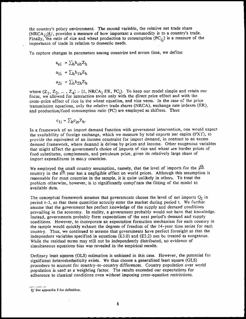
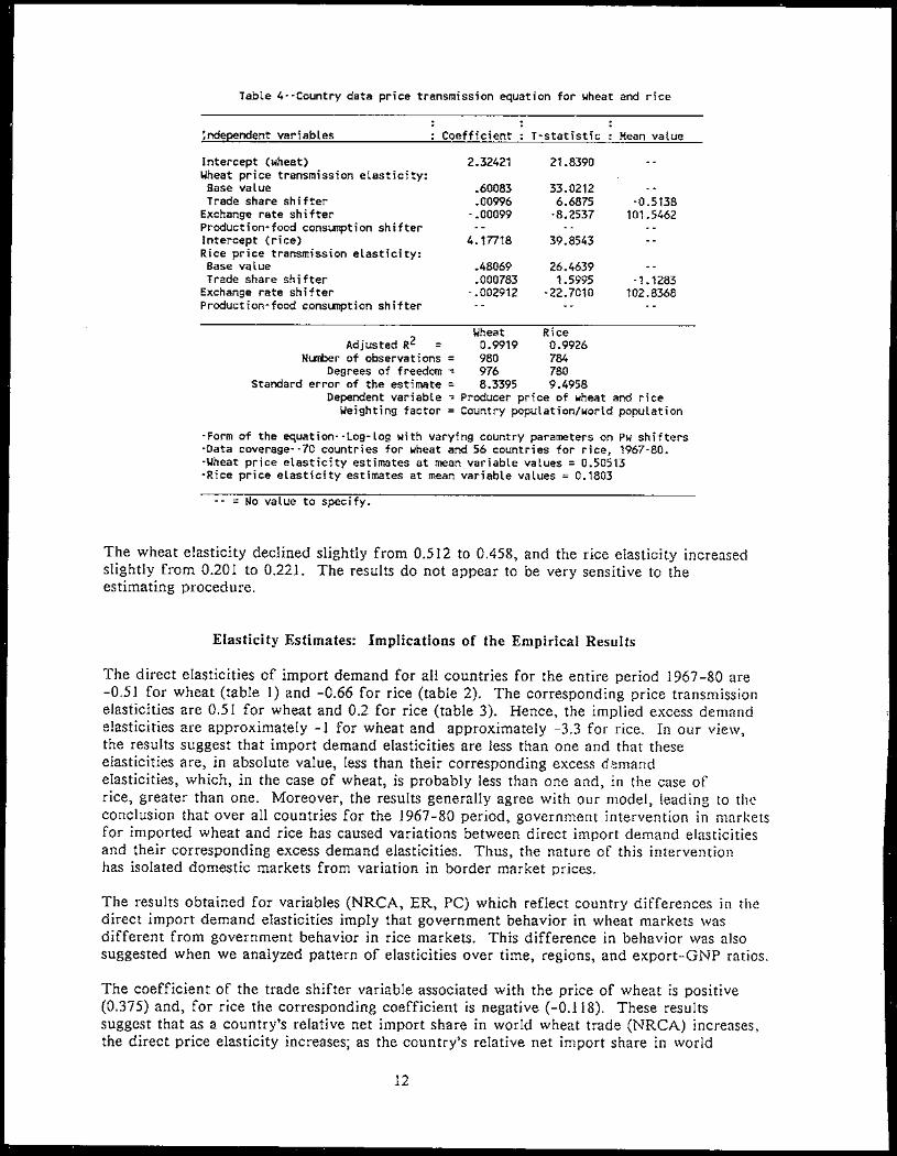
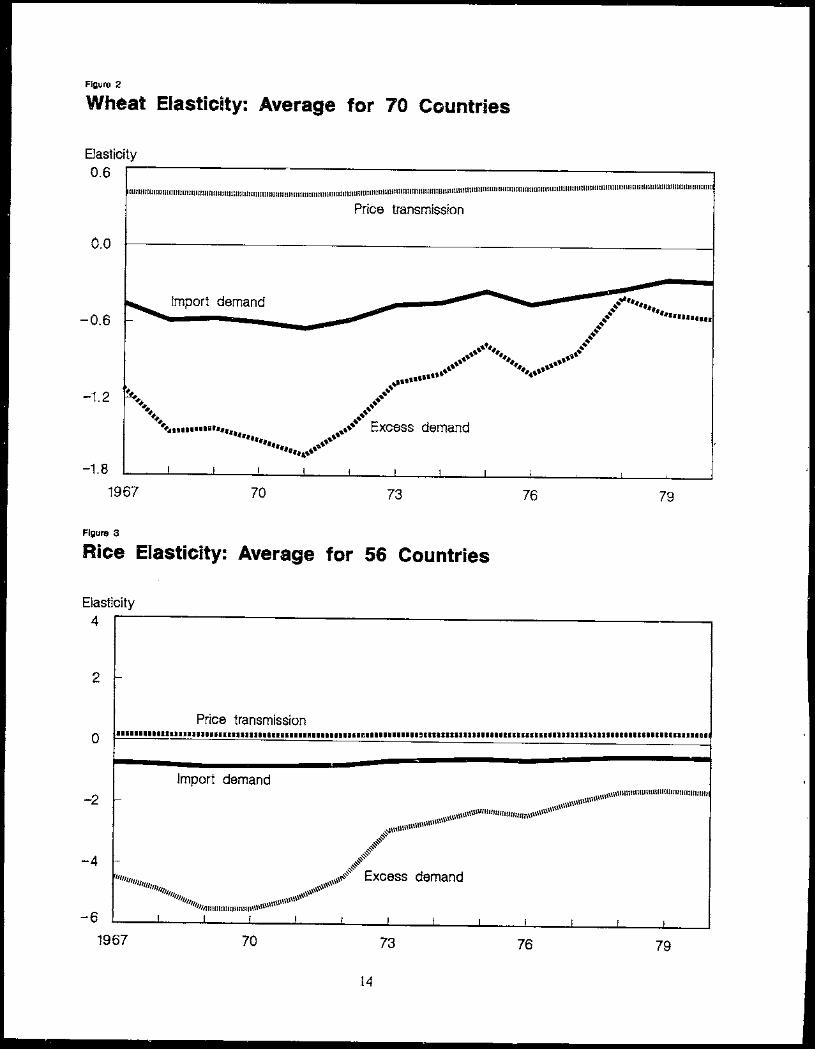
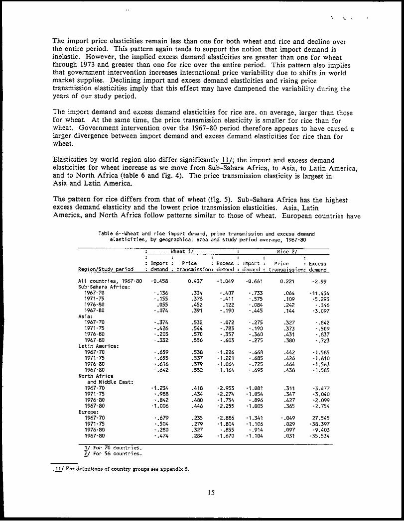
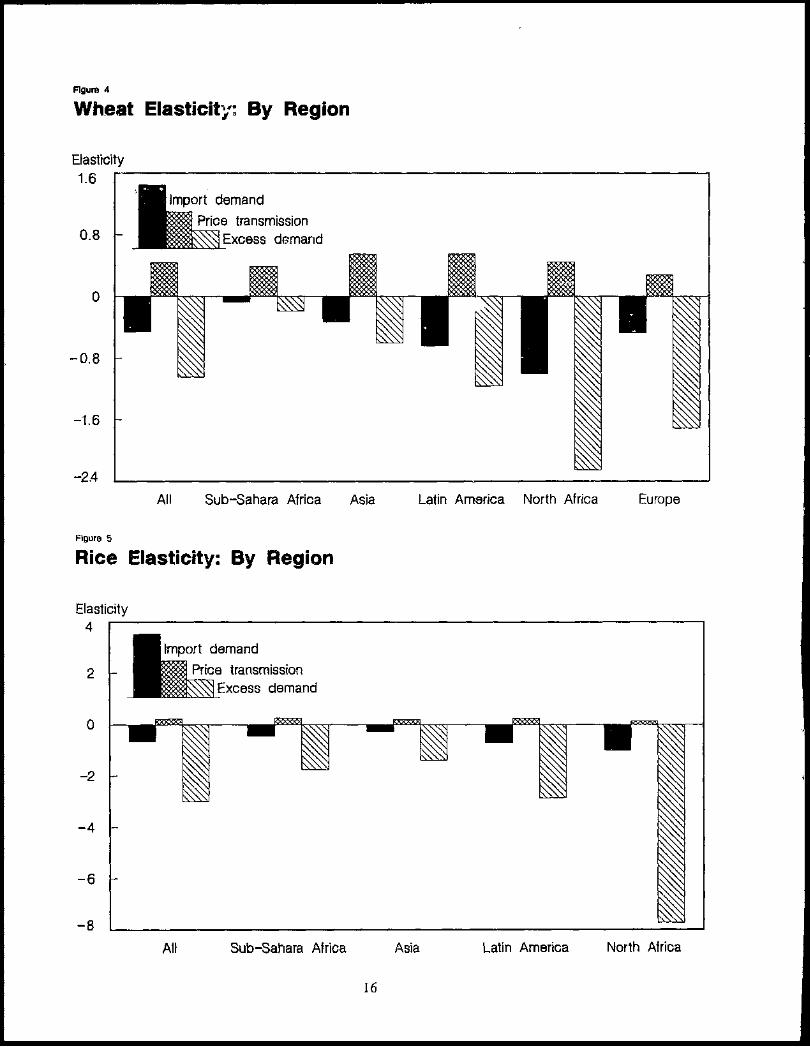

UNITED STATES DEPARTMENT OF AGRICULTURE
ECONOMIC RESEARCH SERVICE
1301 NEW YORK AVENUE N W
WASHINGTON D C 20005-4788
