price response, asymmetric information, and competition … · price response, asymmetric...
TRANSCRIPT

PRICE RESPONSE, ASYMMETRIC INFORMATION,
AND COMPETITION
Joshua Sherman*
Avi Weiss
Abstract
We compare predictions from a theoretical model based on the structure of the main outdoor retail market in
Jerusalem with the results of an empirical analysis of price response to changes in cost. We find that firms without
adjacent competition exhibit both upward and downward price rigidity, an outcome we ascribe to asymmetric
information between the consumer and the firm. Given that previous studies have focused on downward price
rigidities of firms with market power, our findings highlight the importance of accounting for transitory information
asymmetries between the consumer and the firm when studying price rigidity.
JEL Classifications: L11, L13
Keywords: price response, price rigidity, information asymmetry, market power
This Version: October 11, 2012
* Department of Economics, University of Vienna. Email: [email protected] Department of Economics, Bar-Ilan University and IZA. Email: [email protected]
Portions of this paper originated in Sherman’s Ph.D. dissertation in economics at Bar-Ilan University, approved in September 2011, under Weiss’s supervision. We are grateful to Arthur Fishman, David Genesove, and Daniel Levy for many useful discussions and feedback and we thank
Dennis Carlton, Oz Shy, and Wesley Wilson for helpful suggestions and comments. Thanks to Ilan Cohen, Roni Avraham, Shimon Darwish,
Devora Avidan, and Uri Amedi who provided valuable insider knowledge of the Mahane Yehuda market. We are thankful to Yael Landa, Neta Linzen, and Tomer Weil for excellent research assistance. We also thank Pedro Bom, Joe Podwol, Aziz Simsir, Avichai Snir, and Yariv
Welzman for helpful discussions. Comments from seminar participants at the Israel Antitrust Authority, the IO Workshop at Tel Aviv University,
the University of Vienna, and attendees of the 9th annual IIOC and 39th annual EARIE were greatly appreciated. Sherman thanks the Bar-Ilan University President's Scholarship Fund for financial support, and both authors gratefully acknowledge financial support from the Adar
Foundation of the Economics Department at Bar-Ilan University.

1
1. Introduction
Price rigidity has concerned economists for almost a century, beginning with Mills (1927) and
continuing to include the theory of kinked demand (Hall and Hitch (1939), Sweezy (1939)). In particular,
the effect of information transmission on price rigidity has long been a topic of concern in the areas of
industrial organization and macroeconomics. In this paper, we will argue that transitory information
asymmetries between the consumer and the firm influence pricing behavior in ways not previously
considered or examined by earlier studies of price rigidity.
Using a set of daily observations that we collected for approximately four months from Shuk
Mahane Yehuda, the outdoor retail market in Jerusalem and one of the largest such markets in Israel, we
find that firms with localised market power exhibit both downward and upward price rigidity in response
to changes in cost, whereas firms that face immediate competition only exhibit downward price rigidity.
In contrast to previous empirical literature which presents evidence that firms endowed with market power
exhibit quicker upward price response than downward price response, this study indicates that it is
reasonable to expect both upward and downward rigidity on behalf of firms with market power when
short-term information asymmetries exist. And while previous theoretical and empirical studies have
frequently cited information costs or market power as potential sources of price rigidity, this analysis
underscores the relationship between the two phenomena.1
Our findings may be explained by considering our empirical environment, where vendors are
lined up on two sides of a narrow pedestrian walkway. Some of these stands encounter competition for
their product(s) from nearby stands, while others face competition for their product(s) in a different
location of the market, perhaps not within eyesight. First we consider firms that encounter competition
from at least one firm located immediately adjacent or immediately across from the firm in question, firms
which we will refer to as rivals. If these firms are charging the competitive price, when costs increase
their best response is to increase price immediately. When costs decrease, however, these firms may be
able to temporarily collude at last period’s price precisely because of their close proximity to one another
in both geographic and product space.2
A firm without immediate competition, which we will refer to as isolated, naturally charges a
higher price than rival firms due to localised market power. However, the isolated firm’s price is
1 Indeed, Bénabou and Gertner (1993) emphasise this link in their study of how informational costs determine whether inflation variability encourages or discourages search by noting that informational costs imply market power.
2 Such a phenomenon, which is also suggested as a possible explanation for asymmetric price response in previous literature, may be thought of as
focal price coordination or tacit collusion at a focal price. No information asymmetries between the consumer and the firm are required for such downward rigidity to occur. Later in this section we will address the possibility that heterogeneous search costs can explain such downward
rigidity, as suggested by previous theoretical literature.

2
disciplined by the presence of such rival firms.3 When costs rise, the isolated firm is constrained by the
fact that consumers do not yet know that cost has increased. If these consumers observe the isolated firm
increase price above the last period’s price, they will seek to purchase elsewhere. Therefore, the isolated
firm is prevented from raising price until consumers learn of the cost increase. Likewise, when costs
decrease, the isolated firm only lowers price when consumers learn of the cost decrease. Moreover, if
rivals coordinate with one another, the isolated firm may further postpone such a price decrease until
coordination amongst rivals fails.4 Thus the firm without immediate competition exhibits both downward
and upward rigidity whereas the firm with immediate competition only exhibits downward rigidity.
With the configuration of the outdoor market in mind, we will demonstrate the phenomenon just
described in a Hotelling context where one firm is located at one end of the line (A) and more than one
firm is located at the other end (B). In this model, consumers are exogenously located at the ends of the
line (at the entrances to the market).5 Due to its location, the firm at point A may exercise a certain degree
of market power whereas firms at point B cannot. Note that our analysis can also be interpreted more
broadly as a comparison of price response of firms selling a differentiated product (which endows such
firms with a certain degree of market power) with firms that sell a homogeneous product. Alternatively, it
is possible to interpret our study in the context of switching costs, whereby consumers have a particular
level of lock-in for a certain product.
Note that our previous discussion implies that, given short-term information asymmetries,
empirical results of price rigidity should be sensitive to the choice of (or availability of) observation
intervals, a particular concern given that most previous studies use weekly or monthly observation
intervals. For example, suppose that a firm with localised market power (or, in our context, an isolated
firm) is immediately updated regarding changes in its costs, buyers learn of a cost change with a delay of
one day, and price observations are recorded weekly. Given this scenario, the frequency with which the
buyer is updated regarding changes in costs exceeds the frequency of observation intervals. In such a case
it is plausible that short-term downward and upward price rigidities exhibited by the firm would not be
detected by the researcher. Nevertheless, this study does not seek to compare price response using
different observation intervals; it would be difficult to conduct such a comparison using our data given the
3 In a less interesting scenario that is not considered here, the isolated firm will simply charge the monopoly price if it is situated distant enough
from a pair of rival firms. 4 As in the previous paragraph, downward price rigidity related to collusion does not require information asymmetry between the consumer and
the firm. Furthermore, it will be demonstrated that information asymmetry between the consumer and the firm is a sufficient condition for the isolated firm to exhibit both upward and downward price rigidity. However, it will be shown in Section 2 that the cost of travelling from one firm
to another needs to be sufficiently high in order for isolated firms to behave in such a manner.
5 This scenario may be compared to one analyzed by Shy (1996), who considers the case in which one firm is located at point A and one firm is
located at point B, with consumers located at both points. We return to a comparison of the two scenarios in the next section.
3
need for many consecutive observations of a given firm selling a given product, a requirement which we
discuss in further detail later in the paper.
Literature spanning the last three decades has frequently cited market power and search costs as
primary drivers of price rigidity.6 In particular, Carlton (1986) explores the relationship between price
rigidity and concentration and Carlton (1989) discusses how price information asymmetries, amongst
other factors, may contribute to price rigidities. Furthermore, Tirole (1988) and Borenstein, Cameron, and
Gilbert (1997) propose theories of tacit collusion with imperfect monitoring that have been cited as
possible explanations for downward price rigidity.7 Examples of studies that employ search cost
hypotheses to explain price rigidities include Fishman (1996), Yang and Ye (2008), Tappata (2009),
Lewis (2011), and Cabral and Fishman (2012). In particular, Tappata (2009) employs a theoretical
framework in which information asymmetries and the presence of consumers with heterogeneous search
costs lead to quicker upward than downward adjustment. His theoretical model, which predicts a unique
symmetric equilibrium in which price dispersion exists in every period, also predicts that the price
distribution will adjust to costs asymmetrically in relatively competitive environments due to higher
demand elasticity when costs are expected to be low. However, it seems unlikely that heterogeneity in
consumer search costs would be an explanation for downward rigidity of rival firm price response in our
empirical environment. Namely, due to the fact that we have defined rival firms as adjacent firms or firms
immediately across from one another, it is easy for all consumers to compare prices at such firms.
Therefore, we expect that the cost of comparing prices at rival firms is near zero.
Empirical studies have found ample evidence of price rigidity in a variety of markets but typically
do not offer formal theoretical motivation.8 In particular, Peltzman (2000) found asymmetric price
adjustment in two-thirds of the markets he examined and concluded that there is a gap in the standard
economic theory of markets because it does not predict or explain the pervasiveness of the phenomenon.
Meyer and von Cramon-Taubadel (2004), Geweke (2004), and Frey and Manera (2007) provide thorough
6 Wolman (2007) provides a detailed survey of the vast theoretical and empirical literature addressing price rigidity as well as the implications of
such studies for macroeconomic models. The cited literature attributes infrequent price adjustment to one or more of several factors, including
menu costs, relationships between buyers and sellers, and strategic firm behavior. He notes that while earlier empirical work often cites menu costs of price adjustment, more recent literature examining price rigidity has focused on buyer-seller relationships and firm interaction.
7 In particular, the latter study supposes that prices respond immediately upward to cost increases in order to ensure positive margins given higher costs, but respond more slowly downward in response to negative cost shocks in the context of a collusive scheme. It should be noted that this
study offers additional potential explanations for price response asymmetry, including a search theoretic hypothesis as well as a hypothesis which
cites production lags and finite inventories as possible causes. 8 Previously, Geweke (2004) and Eckert (2011) have made this observation with regards to empirical studies of price response in the gasoline
industry. Geweke (2004) notes that while there is a theoretical literature on possible connections between imperfect competition and asymmetric movements in price, this literature does not yet deliver implications that can be tested using available data. Eckert (2011) observes that very few
empirical studies of pass-through using gasoline data present formal models.

4
surveys on empirical studies of price asymmetries.9 Notably, Frey and Manera (2007) find that the vast
majority of studies use data aggregated at the weekly or monthly level. Moreover, a large number of
empirical studies have examined the fuel/gasoline sector.10
For example, a detailed station-level study by
Verlinda (2008) analyzes weekly gas station prices from Southern California and finds that price response
asymmetry is more pronounced amongst firms with relatively more market power.
The paper is divided as follows. Section 2 presents the details and predictions of a theoretical
model based on the Mahane Yehuda market setting in which firms with disparate degrees of market power
compete with one another. Section 3 discusses the Mahane Yehuda market and the data that were
collected. In Section 4 we present the empirical findings and compare these results with the predictions of
the theoretical model. Section 5 concludes.
2. The Theoretical Model
We begin by providing a concise motivation for the theoretical model to be presented in this
section, with a more complete description of the empirical setting presented in the next section. The
Mahane Yehuda market consists of many vendors lined up one next to another on either side of narrow
pedestrian walkways. In practice most vendors sell many goods.11
While some firms face direct and
immediate competition from other stands selling the same goods and are located either immediately
adjacent to one another or immediately across from one another, others are relatively isolated. We define
the former firm type as a rival firm and all other firms are defined as isolated. Rivals interact in a unique
manner because the seller at one rival firm can observe the price that is being charged by the other firm at
all times without having to leave his stand. In addition, consumers incur virtually no cost in order to
compare prices at two such firms. Consumers enter through one of several entrances according to their
9 For example, Hannan and Berger (1991) and Neumark and Sharpe (1992) analyze consumer bank deposit rates and conclude that upward price flexibility and downward price rigidity are a result of market concentration. An empirical study by Kahn, Pennacchi, and Sopranzetti (2005) finds
that banks are quicker to increase auto loan rates in a rising market rate environment than they are to decrease rates when market rates are falling.
In contrast to previous studies, however, they find that banks in more concentrated markets are less likely to engage in such asymmetric behavior than banks in less concentrated markets. This is the first empirical result of which we are aware that finds a greater degree of asymmetry in less
concentrated markets than more concentrated markets. Examples of studies examining agricultural asymmetric price transmission include Ward
(1982), who uses aggregate price data for fresh vegetables, and Aguiar and Santana (2002), who use monthly aggregate retail prices from the city of Sao Paulo, Brazil. Dutta, Bergen, and Levy (2002a) and Levy, Dutta, and Bergen (2002b) examine price rigidities of orange juice.
10 Studies that examine rigidities in gasoline markets begin with Bacon (1991) and Karrenbrock (1991) and continue to include Duffy-Deno
(1996), Borenstein, Cameron, and Gilbert (1997), Borenstein and Shepard (2002), Eckert (2002), Bachmeier and Griffin (2003), Noel (2007),
Balmaceda and Soruco (2008), Deltas (2008), Hosken, McMillan, and Taylor (2008), and Verlinda (2008), amongst others – Geweke (2004) and Eckert (2011) provide thorough reviews of retail gasoline studies.
11 We collected price observations for 10 products in order to protect the researcher’s anonymity and in order to keep the data collection
manageable. While theoretically there may be examples of multiproduct relationships in our empirical setting, we analyze a single product
framework for both theoretical and practical purposes. A single product analysis allows for tractability of the theoretical model, and collecting price observations of more than 10 vegetables in an attempt to capture multiproduct relationships was not feasible and would not have been
informative for our analysis because identifying the correct cost basis for many products was not possible (to be discussed further in Section 3).
5
mode of transportation to the market or by foot according to where they live or work. Store locations are
fixed, and the majority of vendors selling fruits and vegetables have occupied the same space in the
market for a number of years.
With this environment in mind, our theoretical setting is illustrated in Figure 1A. There is one
firm at one end (point A) and firms at the other end (point B) of a Hotelling line that compete in an
infinite-horizon setting, with all firms selling the same homogeneous good.12
The firm at point A is the
isolated firm, the firms at point B are rival firms, and all firms are symmetric.13
At the beginning of each
period, each firm simultaneously chooses a price of the good to be sold that period.14
For simplicity, we
assume that there are two possible costs, and , with . Costs are identical for all firms in a
given period and evolve according to a two-state, first order Markov-switching process where
, , and we assume . In other words, if cost was low
(high) last period, it is more likely that we will observe a low (high) cost this period than a high (low) cost.
There are no fixed costs and the number of firms is given.
Consumers on each side of the market have demand represented by a downward sloping demand
function where is the realization at time of the size of the market, i.e., the number of
consumers in a given period. In every period we assume that consumers only know past cost realizations
and the aforementioned switching probabilities whereas firms know the current and past cost realizations
as well as the switching probabilities.15
Consumers are exogenously located at each point A and B, but
they are not located along the line.16
One may think of these exogenous locations as being determined by
the consumers’ places of residence or employment or mode of transportation, so that consumers who
12 Although one may interpret distance as a measure of product heterogeneity.
13 While we have modeled our theoretical setting using a Hotelling line with two endpoints, one may conceive of analogous settings in which there
are more than two endpoints – one such alternative is presented in Figure 1B. All that is required for our theoretical framework is that rival firms
are located at a minimum of one point and any given point where an isolated firm or rival firms are located is not surrounded by other firms on both sides. If point A and point B for a certain good are each located further inside the market away from an entrance, as in Figure 1B, we simply
account for the distance between the two points. It should be noted that for a given product on a given date, anecdotally it is relatively uncommon
to observe another isolated firm or cluster of rival firms in between a given isolated firm (or cluster of rival firms) and every entrance to that area. This observation will be reinforced by summary statistics regarding the average number of firms per area, reported in Section 3.
14 In Davidson and Deneckere (1986), firms first choose capacities and then engage in price competition. In their model, if firms are not capacity-constrained then the standard Bertrand competitive price prevails. If firms are capacity-constrained, there may be a mixed-strategy solution. In
Mahane Yehuda, a given stand first purchases product at the wholesale market and then sets a retail price. A stand is not capacity-constrained if it
could hypothetically serve all consumers in its geographic area (which is how we will define the geographic “market”) for a particular good. Note that amongst all observations collected there is an average of 3.86 firms selling a given good per area and it appears that these firms are not
capacity-constrained according to the preceding definition.
15 When considering our empirical setting, the current day’s costs (wholesale prices) for vegetables are usually posted on the internet by the Israeli
Ministry of Agriculture in the afternoon of the same market day whereas a consumer must visit the market in order to observe prices (and a given
consumer typically does not visit the market every day). However, as rival firms are Bertrand competitors, their price may also serve as an indication of the current cost if they do not coordinate (to be discussed in more detail later in this section).
16 As will be discussed later in the paper, we define four different areas of Shuk Mahane Yehuda according to product quality and the type of clientele that typically visits each area. Each area has multiple entrance points (typically more than two) and firms primarily compete with other
firms in the same area. Thus, distinct Hotelling lines are located in each geographic area of the market.

6
travel to the other end of the line must return to their original location upon purchasing. A consumer who
travels must incur a travel cost of in order to visit the other point and return to the entrance from which
she entered.17
Note that as no consumers are located in between points, it is optimal for firms to locate at
the entrances, but location is not a choice variable for either firms or consumers. In addition, an equal
number of consumers are assumed to originate at each point A and B in a given period.18
For simplicity we assume two possible demand states, and , where . During the
beginning of the week (Monday – Tuesday) demand tends to be relatively low, whereas during the days
leading up to the Jewish Sabbath (Wednesday – Friday) it is less likely to observe low demand. Thus, we
assume that the probability of a low demand state depends on the weekday. Specifically, given our
empirical environment, we assign a probability of that on Mondays and Tuesdays and a
probability of that on Wednesdays, Thursdays, and Fridays, with .19
The
subscripts and denote the beginning and the end of the week, respectively. In addition, we assume
that demand in each period is realised independently. We also assume that realised demand is observable
to firms and consumers and that both firms and consumers know the probabilities and .
Equilibrium: Rival Firms
There is substantial evidence that firms which are situated within close proximity in both product
and geographic space successfully sustain outcomes that dominate the one-period outcome for at least
brief periods of time, whether they compete in prices or quantities. To this end, we invoke the hypotheses
of Borenstein, Cameron, and Gilbert (1997) and others who have studied oligopolistic price response to
changes in cost, and assume that while explicit collusion may be difficult to attain, oligopolistic firms may
17 While our analysis assumes all consumers share a common travel cost , one might ask whether our result would hold if we allowed for an additional consumer type with no travel cost, which the consumer search literature commonly refers to as a shopper. Sherman and Weiss (2012) examine the relationship between search costs and price dispersion in an empirical study using data collected from Mahane Yehuda during the
same time period. In particular, they explore the possibility that heterogeneities in search costs across geographic areas of the market and over the
course of the week influence the extent of price dispersion observed. After discussing equilibrium behavior of both firm types, we will present two straightforward conditions that are required in order to ensure that the results of our theoretical model are unaffected by introducing shoppers.
18 There are two other obvious competitive scenarios to the one presented here which can also be interpreted in a Hotelling context that are not
considered in this paper, and we note them briefly here. First, one might be interested in analyzing a scenario in which there is a single firm and a
mass of consumers located at each end of the line. Shy (1996) analyzes this precise example and finds that there is no Bertrand-Nash equilibrium
in pure strategies in such a case (but he does show the existence of an undercutproof equilibrium). Such an example is also less relevant for our study because we are primarily interested in how information asymmetries affect price response of firms with differing degrees of market power.
The other obvious example would entail more than one firm and a set of consumers located at each end of the line. As we will see later in the
paper, the ability of all consumers to compare prices without incurring a travel cost render information asymmetries irrelevant in such a circumstance. That is, downward rigidities of firms located at the same point in product space and geographic space may result from collusive
behavior alone. On the other hand, in our analysis information asymmetries between the consumer and firm will be shown to result in downward
(and upward) rigidities of a firm with market power that does not collude.
19 Note that vendors close early on Friday due to the Jewish Sabbath, a detail to be discussed further in Section 3. We ignore three holiday eves in
our theoretical analysis due to their infrequency but we account for these dates in our empirical analysis.

7
be able to coordinate at a focal point, thereby delaying a downward response to cost changes. Note that
the Folk theorem predicts that if the discount factor is sufficiently high, any price between the competitive
price and the monopoly price may be sustained as part of an equilibrium in an environment in which
homogeneous goods firms with identical marginal costs compete in prices over an infinite horizon. We,
however, limit the collusion possibilities to a single focal price. This is appealing as it is essentially
passive (implicit collusion), and therefore allows firms to react rather than to collectively choose a new
collusive price (which would be more profitable than the focal price, but is both more difficult to achieve
and illegal). Therefore, we make the following assumption:
Assumption 1 (collusive price): Collusion can only be attained at the price from the previous period.
In other words, when costs decrease, rivals will seek to earn profits associated with the focal price from
the recent high cost period rather than charging the profit maximizing price, as this price is unattainable.20
Such collusion is supported by the threat of punishment by the other rival firms. Along these lines we
make the following assumption:
Assumption 2 (punishment behavior): If a rival firm deviates from the focal equilibrium, it incurs a
punishment of zero profits in each subsequent period until cost increases.
We assume that the punishment ends when cost increases rather than continuing in every low cost period
into the infinite future. Note that an alternative punishment that included all low cost states into the
infinite future is less realistic and would not alter the substantive conclusions of our analysis.21
If the rival firms are unable to coordinate, they set price equal to marginal cost in that period.
Thus, when , because there is no higher price from the previous period at which the firms
can collude (Assumption 1). Similarly, suppose that and (i.e., rival firms were
unable to coordinate in period ). Then if , it follows that .
Now let us suppose that and . The low cost in the current period coupled with
the high price in the prior period allows the rival firms an opportunity to earn supra-competitive profits by
coordinating at . For this to be an equilibrium, however, it must be the case that no firm has an
incentive to deviate by lowering price in the current period and in turn trigger punishment in future
20 An alternative assumption would be that if the monopoly price is above the prior period price, then the prior period price is the only attainable collusive price, but if the monopoly price is below the prior period price then the parties can collude on the lower more profitable price. This
alternative assumption will not alter the conclusions of the model.
21 That is, a more severe punishment would increase the expected future profits lost due to deviation, thereby shifting the range of parameter
values for which collusion is achievable (the circumstances under which collusion is attainable given our assumed punishment will be discussed shortly).

8
period(s), as per Assumption 2. Thus, cooperation is an equilibrium as long as the single period profit
from defection from the focal, collusive price is less than or equal to the profit from cooperation in the
current period plus expected profits from continued cooperation in subsequent periods.
In Appendix A1 of the paper we demonstrate that our theoretical framework implies that rival
firms will either (1) always collude when cost is low, (2) always set price equal to marginal cost, or (3)
collude following a cost decrease when demand is low, and continue to collude until demand increases or
until cost increases.22
The parameter values associated with each of these three scenarios are also
provided in Appendix A1, and we shall assume parameter values associated with the third scenario for the
remainder of the paper. Given this assumption, we make the following predictions regarding the pricing
behavior of the rival firms:
a) If then
b) If and , then
c) If , , and , then
d) If , , and , then
Equilibrium: The Isolated Firm
We model the interaction between the isolated firm and consumers as a one-shot game. While
firms know the current and past cost realizations, consumers only know past cost realizations (via
information published on the internet or through word of mouth from friends who shopped in previous
periods).23
Likewise, we assume that previous demand realizations are observed by firms and are known
to consumers (also via word of mouth) and the current demand realization is observable to consumers and
firms. Knowledge of this information and the rival firm equilibrium is sufficient for consumers at point A,
the location of the isolated firm, to infer the price set by the rival firms in the previous period. In turn,
they may form prior expectations with regards to the current price of the rival firms.
22 Several studies that have examined oligopolistic behavior in the presence of demand fluctuations provide insight regarding the firm’s ability to collude given observable demand. Rotemberg and Saloner (1986) assume i.i.d. demand and find that collusion at the monopoly price is more
easily achieved when realised demand is low. Later, Haltiwanger and Harrington (1991) assume deterministic demand and find that collusion is
easier to maintain when it is known that demand will rise in future periods. And Bagwell and Staiger (1997) find that the most collusive prices are weakly procyclical when growth rates are positively correlated through time. In each case, collusion is most difficult if future demand is lower
than present demand because it is most tempting for firms to deviate in the current period when they are not deterred by an expected punishment
that will exceed the gains from deviation. While the preceding papers do not allow for price wars but instead predict lower collusive prices in periods when expected future collusive profits are lower, the conclusion given either framework is similar. Namely, given observable demand, we
should expect price to decline when it is more difficult to collude in the current period. This price decrease may be due to a collusion failure or
due to the fact that the collusive price must be lowered in order to maintain collusion in all periods. 23 We will discuss the collection and dissemination of wholesale prices for vegetables in more detail in Section 3.

9
It is straightforward to calculate the expected price of the rival firms in each state of the world
from the perspective of consumers originating at point A. We define Condition 1 as the states of the
world in which consumers at point A know that the rival firms' price equals , and Condition 2 as the
states of the world in which the consumers at point A have ex-ante uncertainty regarding this price. We
further bifurcate Condition 2 into those states in which the previous period cost was low (Condition 2A)
and those in which it was high (Condition 2B). The ex-ante expected prices, denoted , based on the
previous period's cost and price and the current period demand, are summarised in Table 1.24
The isolated firm seeks to charge the price that maximises profit whereas consumers seek the
lowest price, which includes the travel cost d if the consumer chooses to travel to point B. For this
signaling game between the isolated firm and consumers who reside at point A we only consider
sequential equilibria, that is, strategies that are sequentially rational and consistent. Note that for
computational simplicity, we assume that consumers do not travel on the equilibrium path if they are
indifferent between travelling and not travelling.
In the following discussion we shall define ,
,
,
and
. The superscripts and are used to indicate that such prices are the
highest possible prices charged in a separating equilibrium and a pooling equilibrium, respectively, given
the associated current or preceding period cost state realization. For notational purposes, given our
assumption of downward sloping demand, in the following discussion we will periodically refer to
as the quantity that is implied by a particular price chosen by the isolated firm.
Under Condition 1 the isolated firm will choose the lower of two prices – the unconstrained
monopoly price (denoted and
in the low cost and high cost states of the world, respectively) and
the rival firm price plus the travel cost, .
25 Thus, the isolated firm will charge
when
,
when , and no consumers will travel.26
Prices will be equal across cost
states if
. Under Condition 2, pricing behavior of the isolated firm is specified in the following
two propositions.
24 The reader may note that consumers at point B, upon observing a rival firm’s price, may infer if coordination is not possible in period .
They may make this inference according to the value of or an earlier value .
25 Note that since is a measure of the number of identical consumers at either end of the market and marginal costs are constant, the monopoly
prices are independent of . In addition, the ratio between the high cost quantity and the low cost quantity will similarly not be affected by .
Thus, the discussion below is independent of the demand state. 26 Note that if , the isolated firm may undercut the rival firms by charging when and attract consumers from point B. If
such an undercutting strategy yielded greater profits than charging and selling only to consumers at point A, there would be no pure strategy Nash equilibrium. We do not analyze this circumstance here. For more detailed information on undercutproof equilibria, see Shy (1996)
or Shy (2002).

10
Proposition 1 (Pooling Equilibrium): If
given Condition 2 there is a
pooling equilibrium in period in which , independent of the current cost, but there is no
separating equilibrium. Specifically, given Condition 2A the isolated firm always charges
whereas
given Condition 2B the isolated firm always charges
, and consumers do not travel.
Proof:27
First we note that if there is no pooling equilibrium because the highest price the
isolated firm can charge in a pooling equilibrium, , is less than , so the isolated firm will not
sell when cost is high. The consumer, knowing this, will then know that if the product is being sold by the
isolated firm, then the cost must be low, and he will be willing to pay no more than . This accounts for
the lower bound on travel costs.
The condition
guarantees that there is no separating equilibrium. To see this, suppose
that a separating equilibrium exists in which the isolated firm charges when and
when
, and consumers believe this occurs with certainty. This strategy entails the highest price that the
isolated firm would be able to charge in each state without losing any sales from consumers at point A to
the rival firms. Given , when off-equilibrium path profits from charging would exceed profits
generated from charging , and therefore this strategy is not sequentially rational. More specifically,
note that
( ) and
(
). It can then be
shown that when
we have that
. Furthermore, given
that this inequality holds, the same reasoning can be applied to rule out the existence of any other
separating equilibrium. Specifically, if the isolated firm were to charge any price between and when
, off-equilibrium path profits from charging such a price would exceed profits from charging ,
and therefore there is no separating equilibrium in this case.
Now we may check for the existence of a pooling equilibrium. If the isolated firm charges
in both cost states, consumers from point A never travel on the equilibrium path.28
This strategy is
sequentially rational given consumers’ beliefs because given either cost state, it yields higher profits for
the isolated firm than any alternative off-equilibrium path price strategy.29
Lowering price would result in
27 Given Condition 2 consumers from point B never travel because they may infer that the rival firms set price equal to cost based on their
knowledge of or an earlier value . 28 As a technical matter, with regards to the instances in Propositions 1 and 2 in which there is a pooling equilibrium, given Condition 2A we
assume that consumers’ off-equilibrium path beliefs that are greater or equal to , and given Condition 2B we assume that consumers’
off-equilibrium path beliefs that are less than or equal to . 29 Of course in practice one may observe customers travel in between two firms selling the same good in our empirical setting or other empirical settings for a variety of reasons. For example, in the market, there are also cafes, restaurants, and vendors that sell durable goods. In addition,
some consumers may not share the same travel costs. We assign a common travel cost of to all consumers for simplicity and because we seek to

11
strictly lower profits whereas raising price would cause consumers to travel in both cost states, resulting in
zero profits.30
Proposition 2 (Pooling and Separating Equilibria): If
given Condition 2 there exist
both pooling and separating equilibria. Consumers do not travel in any equilibrium.
Proof: In this case
, so in a separating equilibrium the isolated firm will
charge
in the low cost state of the world,
in the high-cost state of the
world, and consumers do not travel. Given these beliefs by consumers, a separating equilibrium is
sequentially rational because profits are always higher from choosing these prices than from choosing any
alternative off-equilibrium path pricing strategy.
In addition, as in Proposition 1, a pooling equilibrium also exists in which is
charged. This pooling equilibrium is sequentially rational given consumers’ beliefs because for each cost
state it yields higher profits for the isolated firm than any alternative off-equilibrium path price strategy. It
is easy to see that lowering price would result in strictly lower profits regardless of whether or
is charged. Raising price would result in strictly lower profits when , whereas
raising price when would cause consumers to travel in both cost states and result in
zero profits.
To summarise, Propositions 1 and 2 show that there is always a pooling equilibrium in which the
isolated firm’s price is independent of the current period’s cost when , while a separating
equilibrium only exists when the travel cost is high (because, for instance, the isolated firm is sufficiently
distant from the rival firms such that the rival firms exert little or no competitive pressure on the isolated
firm). However, whenever a separating equilibrium exists, a pooling equilibrium exists as well.31
Our
demonstrate that heterogeneous search costs are not necessary to generate downward and upward price rigidities. However we briefly address the ramifications of allowing some consumers to have no travel costs at the end of this section.
30 Trivially speaking, given downward sloping demand, consumer surplus and total welfare are lower when consumers learn with a delay
(which results in a pooling equilibrium) relative to a scenario in which consumers and firms are contemporaneously informed of in period . 31 Returning to footnote 17, if we were to introduce a second consumer type that did not have any travel costs (shoppers), it is easy to see that our predictions regarding equilibrium behavior would not change given Condition 2A or 2B. Namely, since rival firms price at marginal cost given
either condition, the isolated firm cannot undercut the rival firms in order to attract shoppers and therefore it will simply sell to those consumers at
point A with a travel cost of at the prices predicted in this section. Given Condition 1, we note that both the incentives for rivals to collude as well as the incentives for the isolated firm to not undercut the rivals are altered when shoppers are introduced into the market. However, our
predictions should not be affected if two conditions hold. First, rivals’ focal price collusion remains more profitable than deviation given the possibility of attracting all consumers located at point B plus shoppers at point A. Second, the isolated firm earns higher profits from charging
when and
when to consumers at point A who have a travel cost than from undercutting the
rival firms’ price of by a small amount and attracting all consumers at point A as well as shoppers from point B. Given , , and , it would be straightforward to find a proportion of shoppers at points A and B such that both of these conditions are satisfied, namely a proportion of
shoppers that is relatively low. However, addressing this scenario formally is beyond the scope of this paper.

12
theoretical predictions are summarised in Table 2, and we will return to these predictions once again prior
to examining our empirical results in Section 4.
3. The Data
Located in the commercial centre of western Jerusalem, the market dates back to the late 19th
century and subsequently evolved into a permanent market during the late 1920’s and 1930’s. The market
underwent renovation in the early 2000's and today is one of the largest in Israel, featuring hundreds of
vendors of vegetables, fruits, meats, poultry, fish, baked goods, and clothing.32
Vegetable and fruit
vendors constitute the largest percentage of sellers, however the market’s gentrification in recent years is
evidenced by the entrance of several small coffee houses and restaurants into the market.33
Regular observation of the market as well as discussions with various vendors and the market
manager served to inform us as to how one might classify areas of the market according to quality
observed. Accordingly, we divide the market into four areas, A through D, where A is the highest quality
area and D is the lowest quality area. As can be seen in Figure 2, Areas A-D are geographical
distinctions.34
For example, the southern area of the market features the highest quality products and is
typically the most expensive.35
This area is closest to the parking lots, where presumably higher income
consumers arrive by car. The northern areas of the market, on the other hand, are typically less expensive.
Due to local traffic patterns, consumers who arrive by bus typically enter through one of the northern
entrances of the market. While one might suggest alternate ways of defining geographic markets in this
setting, distance-based measures will necessarily be misleading because they would not take into account
abrupt changes in lighting and cleanliness of the environment, for example, which essentially signal
differences in the quality of product sold. Temporal variations in quality appear to affect the entire market
32 In 2012 the market published an official website in Hebrew and English at http://www.machne.co.il/en/. The site includes a map, photos,
videos, and a very partial list of vendors. Given that the market features hundreds of vendors, the website’s list of vendors is extremely limited
and does not include most fruit and vegetable vendors. 33 Most owners only own one stand and most renters rent only one stand. In rare cases an owner may own two stands. The exception to this rule
may be observed in the northern area of the market, where an adjacent school owns approximately 20 store spaces, most of which are rent-controlled and occupied by disparate sub-owners. However, it is not uncommon for cousins or even siblings, for example, to operate competing
stores. We were unable to learn which vendors are related with whom, but we were told by market insiders that many of these familial
relationships are adversarial. So while we cannot account for familial relationships in our analysis, the anecdotal evidence leads us to believe that strategic pricing decisions are generally made without regard to familial relationships with competitors.
34 There are three firms that are not in the immediate vicinity of the other firms in Area D but are classified as Area D firms due to the extremely low quality of product that they sell. However, no observations of these firms are included in our empirical analysis using two wholesale price
change lags because they do not meet one or more of the restrictions that we impose for inclusion in the analysis (such as posting price during all
periods for which wholesale price changes are included as explanatory variables). These restrictions will be explained in detail at the beginning of the next section.
35 In Section 4 we will present simple empirical evidence of price differences across geographical areas.

13
to the same degree and the index of quality throughout the market does not appear to change over time.
Therefore our analysis should not be influenced by cross-sectional or temporal quality differences.
One may also note from Figure 2 that there are several entrances into the market and into each
area. Typically there are no more than three firms selling a particular product in between two entrances to
a given area of the market, but given that there are several entrances to a given area, it is common to find
more than three firms selling a particular product in a given area, as can be inferred from Table 3 (which
excludes Sundays for reasons specified in the next paragraph). Given that firms principally compete with
other firms in the same area, when considered in the context of the theoretical model in Section 2, distinct
Hotelling lines are located in each geographic area of the market.36
In addition, it is typically not the case
that there is another isolated firm or cluster of rival firms in between a given isolated firm (or cluster of
rival firms) and every entrance to that area (for a given product on a given date). Summary statistics
reported in Table 3 coupled with the fact that every area except for Area D has more than two possible
area entrances (see Figure 2) serves as further evidence for this observation.
The market is open six days a week, Sunday through Friday (it is closed on the Jewish Sabbath
and holidays). Sunday is by far the lightest shopping day of the week and therefore many stores are
closed. In addition, some stores that do open on Sundays sell lower quality leftover produce from the
previous week on particular dates rather than purchasing new product from the wholesale market. On
other dates, the same stores may sell fresh product. Therefore, Sunday prices at the retail market are often
unrelated to the price recorded that morning at the wholesale market. 37
In addition, when incorporating
Sundays, price change observations from Friday to Monday are lost for the relatively large number of
firms that close on Sundays. For these reasons we will omit Sundays from the empirical analysis and treat
Friday and the following Monday as consecutive market days.
Our dataset combines hand-collected daily price observations from the market between April 2,
2009 – August 4, 2009 and the corresponding wholesale price data for the same period, which we discuss
shortly.38
Specifically, every day we observed which of the following products a given firm was selling
and the associated price of the product, when posted: beets, cauliflower, corn, cucumbers, kohlrabi, red
36 As illustrated in Figure 1B, two or more particular entrances to a given area need not be literally connected by a straight line in order to compare
the theoretical predictions presented in Section 2.
37 As discussed below, much of the produce sold to consumers on Fridays, which is a short day, are purchased by the retailers on Thursday. 38 We note that were no major unanticipated shocks to demand during the observation period. The rainy season ended before the beginning of the
observation period and the weather was warm in the spring and hot in the summer, as is typical for Jerusalem. Also, there were no security incidents in the area surrounding the market during the data period. Construction on a main street next to the market, Jaffa Road, began well
before the data period and continued throughout the data period – therefore traffic patterns were the same throughout the data period.
14
cabbage, red bell peppers, sweet potatoes, white cabbage, and yellow bell peppers.39
Observations were
collected between 10:00 a.m. – 12:00 p.m. as it is during this period that prices are the steadiest prior to
declining in the late afternoon.40
We chose to restrict the analysis to vegetables because we sought to
match retail prices of non-durable, unpackaged products with reliable daily cost data for the same
products. Thus, we excluded fruits because many fruits were subject to Jewish sabbatical year laws
during the data collection period and also because most fruits can generally be stored longer than
vegetables, which may have created a problem of relating the correct cost basis to a given day’s product.
Also, each vegetable chosen has only one type sold in both the wholesale and retail markets and therefore
the retail data for these products could be easily connected with corresponding wholesale data.41
We observe one marginal cost component of the firm – vegetable wholesale price – and this
component accounts for the majority of the firm’s marginal costs. Wholesale price data were obtained
from the Israeli Ministry of Agriculture, which reports daily “common,” “high,” and “low” wholesale
prices by product type and by quality for the Tel Aviv, Jerusalem, and Haifa wholesale markets.42
Large
transactions occur at or very near the common price, and smaller transactions occur at the high price, for
the same quality. Produce sold at the low price tends to be lower quality produce or mixed quality or
mixed produce types. We therefore use the common price as the wholesale price facing retail vendors.
The Ministry of Agriculture does not record wholesale prices on Fridays even though the wholesale
market is open. However, most Mahane Yehuda vendors do not purchase at the wholesale market on
39 Vendors were generally not asked about non-posted prices in order to preserve the researcher’s anonymity – Table 3 indicates the number of
observations for which price was posted out of all observations that were collected (excluding Sundays). In addition, unlike the bazaar economy
in Morocco described by Geertz (1978), customers typically do not negotiate with vendors on price. In Israel, vendors at flea markets and stores selling durable goods to tourists are much more likely to engage in negotiation. As an article in Ha’aretz, one of Israel’s daily newspapers
reported, “Many people are under the impression that shuk (market) equals haggling. But believe it or not, your wiles are better put to use in the
staid-looking judaica and jewelry shops (read: tourist traps) in the Ben Yehuda pedestrian mall in the center of town, or at the Arab shuk in the Old City, than at Mahane Yehuda.” Shoshana Kordova, “Playing the Market / Mahane Yehuda,” Ha’aretz English edition. February 28, 2005. In
three studies of markets for fruits and vegetables, Kirman et al. (2005), Moulet and Rouchier (2008) and Kirman, Moulet, and Schulz (2008)
examine bargaining and price discrimination, respectively, at the wholesale market for fruits and vegetables in Marseilles. The dynamic described between buyers and sellers at the wholesale market for fruits and vegetables is significantly different from the interaction between buyers and
sellers at a retail market for fruits and vegetables due to the fact that the wholesale market features professional buyers.
40 The current manager of the market informed us that during the 1980’s he uncovered a cartel supervised by three to four vendors. These vendors
would regularly circulate through the market and convey a specific glance to the other vendors which would indicate whether their prices were too
low. According to the manager, this cartel was eventually broken over a period of several years as there was eventual turnover of vendors.
41 The market is characterised by a large number of vendors in very close proximity. Occasionally, the dividing line distinguishing one vendor
from another was not discernible to the researcher, and this became particularly difficult when vendors which typically did not sell products that
we tracked chose to sell a tracked product for a period of only a day or two. As noted earlier, vendors were typically not asked about these products in order to preserve the researcher’s anonymity, a concern given that on occasion certain vendors questioned whether the researcher was
tracking prices. Such observations accounted for 350 out of 12,333 posted and non-posted price observations (excluding Sundays), and therefore
these observations are excluded from our analysis. However, after imposing consecutive period posted price and firm status restrictions that we discuss at the beginning of the next section, only nine such observations had to be removed from our empirical analysis. In extremely rare cases,
one stand sold a particular product at two different posted prices due to obvious quality differences. The lower priced product was likely product
that did not sell out from the prior day. These lower priced observations were not recorded by the researcher. In all other cases, firms post one price per product or choose to not post price. Due to oversight, one stand that never had rivals and which typically sold sweet potato was
occasionally missed. In addition, there was one stand that was noticed after data collection began. Once noticed, it was learned anecdotally that
this stand hardly ever posted price for its products nor did it ever have rival stands. Therefore its omission should not affect the analysis. 42 This convention is also used by European governmental agencies and private firms for reporting European wholesale market prices.

15
Fridays – Friday is a shortened market day due to the Jewish Sabbath and Friday’s product is typically
purchased by Mahane Yehuda vendors on the previous day. The same is true with respect to holiday eves.
Therefore, we assume that retailers use Thursday morning’s wholesale price as their marginal cost basis
for Thursday and Friday (the same procedure is applied to holiday eves).43,44
While the Mahane Yehuda retail market in Jerusalem serves thousands of consumers every day,
the Jerusalem wholesale market serves many other small to medium sized stores in and surrounding
Jerusalem and therefore we consider the Jerusalem wholesale price to be exogenous to prices observed at
the retail market.45
In Figures 3A – 3J we display graphs of the wholesale price and the average daily
retail price over time for the ten products for which we collected price observations. Perhaps the most
peculiar pricing behavior is exhibited in Figures 3G (red peppers) and 3J (yellow peppers), where we
notice that the wholesale price exceeds the average retail price during particular periods. However, when
examined by geographic area, we find that on average, margins are negative only in lower quality areas of
the market.46
This likely indicates that the wholesale price level for these particular firms is actually lower
than the common wholesale price recorded by the Israeli Ministry of Agriculture. However, this should
not influence our analysis given that we assume that wholesale price decreases and increases have a
uniform effect on products of different quality levels.
4. Empirical Results
In order to test our theoretical model in which firms compete as either an isolated firm or as a rival
firm for several consecutive periods, we run regressions that include two wholesale price change lags. In
43 There are two key differences between Sundays and Fridays for purposes of our empirical analysis. First, a substantially larger number of vendors are open on Fridays relative to Sundays due to very low demand on Sundays. Second, the decline in quality in Fridays is largely uniform
across vendors whereas the vendors that do sell on Sundays may sell fresh product on one date and leftover product from the previous week on
another date, further complicating analysis of pricing behavior on Sundays. 44 There were 10 dates which did not fall on a Friday for which a wholesale price was not recorded by the Ministry of Agriculture for the
Jerusalem wholesale market. In such instances, an estimated Jerusalem wholesale price was used. This estimate was calculated according to the percentage change in price observed at an alternate wholesale market from the last day for which the Jerusalem wholesale price was available to
the date of the missing Jerusalem observation. The alternate observations used to make this calculation were considered in the following order
(based on the existence of such an alternate observation): the Ministry of Agriculture Tel Aviv wholesale market price, the Ministry of Agriculture Haifa wholesale market price, and the Plants Board Tel Aviv wholesale market price. The same calculation was performed in the
extremely rare instance in which an observation for only one particular product was not taken by the Ministry of Agriculture.
45 It should be noted that some product that retailers bring to market is not purchased at the Jerusalem wholesale market. There are a few vendors
that receive their product directly from the West Bank, and this product is typically less expensive than product sold at the Jerusalem wholesale
market. However, if we assume that wholesale price trends affect a given product equally regardless of where the product was purchased, then wholesale price changes in the Jerusalem wholesale market likely occur in the same direction and with similar magnitude to wholesale price
changes for the same product bought elsewhere. The same reasoning would apply to the rare occasion when a retailer buys from the Tel Aviv
wholesale market or if he receives product directly from a farmer rather than purchasing at the Jerusalem wholesale market. 46 For red peppers, the average daily margins (standard deviation) in Areas A-D using the daily common wholesale price reported by the Israeli
Ministry of Agriculture are: 0.58 NIS/kg (1.51), -0.25 NIS/kg (1.78), -1.67 NIS/kg (1.63), and -1.94 NIS/kg (1.81). For yellow peppers, the average margins in Areas A-D using the common wholesale price reported by the Israeli Ministry of Agriculture are: 2.53 NIS/kg (1.21), 1.19
NIS/kg (1.50), -0.08 NIS/kg (1.87), and -0.55 NIS/kg (1.20).

16
determining the number of lags of wholesale price change to include, we had to balance between omitting
observations and omitting potentially relevant information pertaining to the observations themselves. In
our case, it is particularly difficult to compare different lag specifications because the addition of each
successive lag results in a notable reduction in sample size due to our requirement of successive price
observations and constant firm status. Namely, in order for an observation to be included in a
specification for which there are two wholesale price change lags, it is necessary for a firm to post price in
four consecutive periods and retain its status as an isolated firm or rival firm during these four periods.47
In our analysis we will also run a robustness check in which only one wholesale price change lag is
included, and differences in sample size will be reported when addressing our results using different lag
lengths.
Recall from the theoretical model in Section 2 that whereas rival firms are disciplined by one
another, the isolated firm is disciplined by rival firms. Therefore it is important that the isolated firms that
we observe in our empirical environment compete in the same geographic area as rival firms.
Accordingly, we conduct our empirical analysis by analyzing three different subsets of our dataset. After
imposing the consecutive period firm status and lag restrictions outlined in the previous paragraph, our
first subset (Subset 1) includes all eligible observations of rival firms but only some price observations of
isolated firms; specifically, we exclude observations of isolated firms if no rival sold the same product
during the same period and in the same geographic area. Given the criteria for inclusion described in the
previous paragraph, this implies that isolated firms included in the first subset of observations post price
for four consecutive periods, and throughout these four periods at least one rival firm also sold the same
product in the same geographic area. We restrict our second subset (Subset 2) by product rather than by
the competitive environment. Specifically, given all observations that meet the consecutive period firm
status and lag restrictions, we analyze a subset of products for which rival firms account for at least one
quarter of the observations in at least one of the geographic areas (see Table 4). Our rationale for this
subset is that consumers first encountering an isolated firm selling these products are more likely to expect
that rival firms also sell these products on the same day. This expectation in turn may influence the
isolated firm’s pricing behavior even if rival firms do not sell on that particular day. Our third subset of
observations (Subset 3) combines these restrictions.
One immediate theoretical expectation is that price charged by isolated firms should be higher
than that charged by rival firms, ceteris paribus. We perform a simple check of this prediction by running
a pooled OLS regression (Equation 1) of price observations in each of our three subsamples, where
denotes the firm, denotes the good, and denotes the date. In addition, the current period wholesale
47 We briefly discuss the potential for selection bias later in this section.

17
price for a given good is denoted as , assumes a value of one if a rival of firm f sells the
same product in the same period, and the default cases for weekday, area, and product are Wednesdays,
Area B, and cucumbers, respectively:
∑
∑
∑
As expected, the results (Table 5) indicate that isolated firms price higher than rival firms.48
We
also notice that prices are lowest on Fridays and descend in order from Area A through Areas B - D.
Lower prices on Fridays are likely due to quality differences, as most of the produce would have been
purchased a day earlier. In addition, firms may charge lower prices in order to ensure that they will sell
out prior to the weekend. Note that no observations of cauliflower or red cabbage qualify in any of the
three subsets. Also note that there are fewer than 50 observations of beets, corn, kohlrabi, sweet potato,
and white cabbage in Subset 1 and fewer than 50 observations of corn and sweet potato in Subset 3.49
We recall from Table 2 that the timing of the response to cost changes depends not only on the
direction of the change and on the type of firm; it also depends on the level of demand. Specifically,
collusion is only maintained when low demand is realised and therefore empirically we would expect
retail prices to adjust downward to wholesale price decreases more often when it is less likely to observe
low demand – on Wednesdays, Thursdays, and Fridays (which we denoted as Period E days in our
theoretical model). Therefore, using the predictions of Table 2, it possible to infer the periods in which it
is likely to expect price to respond to a cost change according to weekday of the cost change. Table 6
offers an interpretation of variables that we will use for the remainder of our empirical analysis, and Table
7 includes predictions of price response for specifications in which two wholesale price change lags are
included. Our predictions in Table 7 assume an actual value of from Section 2 such that only a pooling
equilibrium exists for isolated firms; the existence of a separating equilibrium would require a sufficiently
large value of such that rival firms exert little or no competitive pressure on the isolated firm. However,
as outlined in Proposition 2, it is worth recalling that a pooling equilibrium also exists given such a
sufficiently large value of .
48 We cluster standard errors at the date product level throughout our analysis in order to allow for correlation across vendors selling a given
product on a particular date. We have 215, 281, and 175 unbalanced clusters at the date product level in Subsets 1, 2, and 3, respectively. Clustering at the firm level yields insignificant results for the rival coefficient estimate in Equation 1, however, clustering at the firm level using our data is problematic because we have only 38, 38, and 34 unbalanced firm clusters for Subsets 1, 2, and 3, respectively whereas the estimator is
asymptotic in the number of clusters.
49 Subset 1 contains the following number of observations by product: beets (19), corn (27), cucumbers (989), kohlrabi (25), red peppers (326), sweet potato (46), white cabbage (18), and yellow peppers (22). Subset 2 contains: corn (58), cucumbers (1,100), red peppers (562), and sweet
potato (275). Subset 3 contains: corn (27), cucumbers (989), red peppers (326), and sweet potato (46).

18
Given our predictions in Table 7, we may now test our theory by formulating an error correction
model. The model includes current and lagged downward and upward wholesale price changes interacted
with firm type in order to examine the speed and magnitude of isolated firm and rival firm price response.
In addition, weekdays are interacted with wholesale price changes because we expect downward price
response to vary by weekday, as predicted earlier.50
Previous period retail price and wholesale price are
included to capture current period adjustment to the long term relationship between the two variables, and
lagged retail price changes are included to account for short term price adjustments:
∑
∑
∑
∑
∑
∑
∑
∑
The sample is an unbalanced panel of observations collected over a period of 82 dates.51
Note
that there are six market days examined – Mondays, Tuesdays, Wednesdays, Thursdays, Fridays, and
holiday eves, but only four mornings on which wholesale price may change – Mondays, Tuesdays,
Wednesdays, and Thursdays.
Given our interest in immediate and delayed retail price response on different weekdays for each
firm type, in most cases it is difficult to interpret the results of Equation 2, which are reported in Appendix
A2, without performing -tests on the sums of coefficients. For this reason in Table 8 we report the
magnitude and significance of retail price response of isolated firms and rival firms to changes in
wholesale price according to the weekday of the wholesale price change. Estimates are calculated by
summing the appropriate coefficients found from estimating Equation 2.52
For example, in order to
calculate the estimate of isolated firm second period response to a wholesale price decrease
that occurred on Monday, we sum
. In
Appendix A2, this corresponds to summing the coefficient estimates associated with and
50 The specification that we describe does not include interactions between wholesale price change, firm type, and weekday due to sample size
considerations, an issue which we will address shortly. However, results of a specification that includes these interactions, which are similar, will be reported and discussed later in this section.
51 Selection bias should not be a concern because while the profitability of a firm selling a product in a given period may affect the probability of that observation appearing in the sample, one would not expect profitability to explain a change in price, the dependent variable of interest in our
study.
52 Note that isolated firm price response on Wednesdays, the base case, occurs in period for a wholesale price change on Wednesday, period
for a wholesale price change on Tuesday, and period for a wholesale price change on Monday.

19
(0.280 – 0.201 in Subset 1, for example). Rival firm second period response to a
wholesale price decrease that occurred on Monday would be
calculated as
. In Appendix A2 this corresponds to adding the coefficient
estimates associated with ,
, and (0.280 –
0.201 + 0.076 in Subset 1, for example), recalling that implies rival status during the current
and preceding three periods. For these estimates, the values in parentheses are p-values associated with -
tests that the sum of the corresponding coefficient estimates from Equation 2 are equal to zero. Table 7
lists each calculation required to compute the estimates reported in Table 8. We also report estimates of
robustness checks of Equation 2 in Tables 9A – 9D, which we will discuss shortly.
First, let us compare the results of Table 8 directly with our predictions in Table 7. Examining
rival firm and isolated firm upward response, our results indicate that rival firms respond upward
immediately to positive cost shocks on all weekdays except for Thursdays
. On the other hand, isolated firms only exhibit significant immediate
upward response on Mondays . In addition, isolated firms exhibit
significant upward response on Wednesday to positive cost shocks that occur on Tuesday as well as
significant upward response on Thursday to positive cost shocks that occur on Wednesday
. Further evidence of differences in first and second period
upward response between isolated firms and rival firms is offered in Appendix A2 by the positive
coefficient estimates of (significant at the 10% level in two of the three subsets) and
by the negative coefficient estimates of (significant at the 10% level in all three
subsets). These findings are mostly consistent with our theory, which predicts that when costs increase, it
is a best response for rivals to increase price immediately if they could not successfully collude in the
previous period. In addition, if a separating equilibrium is not a sequential equilibrium, as outlined in
Proposition 1 earlier in the paper, then isolated firms will choose price independent of the current cost
state in a strategy consistent with a pooling equilibrium. In particular, in a pooling equilibrium we predict
that an isolated firm will raise price one period after a cost increase.
In addition, we notice in Table 8 that neither firm type exhibits significant immediate downward
response on any weekday except Monday. Isolated firms’ immediate response to both wholesale price
increases and decreases on Mondays is interesting and may reflect the fact that the period between
Thursday and Monday allows consumers ample time to learn of a cost change, whereas a normal 24 hour
period from one weekday to the next is not sufficient for most consumers to become informed. We should
note, however, that our results for Mondays are somewhat problematic in general due to the fact that

20
Sunday observations are omitted from the analysis for reasons stated earlier. Thus it is possible that our
theory cannot be appropriately tested on Mondays.
Given that our theory predicts no immediate downward response by isolated firms when only a
pooling equilibrium exists, the fact that isolated firms’ immediate downward response is insignificant on
Tuesdays, Wednesdays, and Thursdays is as expected. We also note that we would expect rivals to
respond downward immediately when low realised demand is less likely, on Wednesdays and Thursdays.
We do not observe this immediate downward response on either day, however in Subset 3 we only have
28 period rival observations (and eight date product instances) that occur when wholesale price
decreases on a Wednesday. This is shown in Table 10, where we summarise the number of observations
in Subset 3 according to firm type, weekday, direction of wholesale price change, and number of lags.53
In Table 8 we do find evidence of simultaneous delayed downward response by both firm types
on Wednesday. This can be seen by noting the positive and significant estimated coefficients of
and due to a wholesale
price change on Tuesday. This finding is consistent with our prediction that coordination is likely to break
down on Wednesday, as discussed earlier. On the other hand, we do not observe significant delayed
downward response of isolated firms on Thursdays and Fridays. It is possible that we do not observe
delayed downward response of isolated firms on Friday due to a wholesale price decrease on Thursday
because quality is observed to be lower on Friday, and therefore prices decrease significantly on Friday
independently of a wholesale price decrease (see the coefficient estimate of in Appendix A2).
We perform several robustness checks on Equation 2 using the third subset of data, and we report
these results in Tables 9A – 9D. We note that the inclusion of interactions (Table
9A), removal of the error correction terms (Table 9B), removal of both the error correction terms and
lagged retail price changes (Table 9C), and specification of the regression using only one wholesale price
lag (Table 9D) do not alter the results considerably (note that using only one wholesale price change lag
increases the number of observations in Subset 3 from 1,388 to 1,760). Our motivation for the robustness
check reported in Table 9A relates to our prediction in Table 8 that rivals will respond downward
immediately (and therefore one period ahead of isolated firms) on Wednesday and Thursday. Therefore
the difference between isolated firm and rival firm downward response in periods and due to a
wholesale price decrease on Wednesday or Thursday should be different than the difference in downward
response on Mondays or Tuesdays. However, including interactions (Table 9A) in
order to allow for the difference between isolated firm and rival firm price response to vary by weekday is
53 In Tables 9A-9D and Table 10 we only report results and summary statistics from Subset 3, the subset with the smallest number of observations,
for space considerations.

21
somewhat problematic due to the relatively small amount of observations for particular combinations of
firm type, weekday, and negative or positive wholesale price change (shown in Table 10).
Notwithstanding these issues, an -test that all coefficients are equal to zero cannot
be rejected at the 10% level, and the results in Table 9A are similar to those reported in Table 8.54
Next, we check whether three-day cumulative responses of isolated firms and rival firms are
significantly different than zero by weekday of the wholesale price change (Table 11). Given our theory,
we should observe significant downward and upward three-day cumulative response due to wholesale
price changes on all weekdays. While this is observed in all cases on Mondays and Tuesdays and in some
cases on Wednesdays, the fact that no significant cumulative response is observed due to a wholesale price
change on Thursday may be due to the characteristics of period observations (Fridays, when prices
decline due to lower quality) and period observations (Mondays, which occur several days later).
Now that we have examined the periods for which isolated and rival firm price response is
significantly different than zero (Table 8) as well as the significance of three-day cumulative price
response, we report results of additional tests of our coefficient estimates found from Equation 2. In
particular, we examine three-day cumulative price response of isolated firms vs. rival firms in both
directions and three-day cumulative downward price response vs. three-day cumulative upward price
response of both firm types. Table 12A presents each test and its predictions and Table 12B presents the
results.
Given that isolated firms presumably possess relatively more market power than rival firms, we
would expect their price-cost pass through in both directions to be relatively smaller than rival firms
( and
. However, we only find that cumulative response of isolated firms is significantly
different than cumulative response of rival firms due to downward wholesale price changes. In examining
cumulative downward response vs. cumulative upward response of both firm types ( and
,
we do not reject the null hypothesis of equality between three-day cumulative downward response and
three-day cumulative upward response of either firm type. We also test but do not report per-period
downward and upward equality of coefficient estimates by firm type. We do not reject equality of
downward and upward first period response of isolated firms on any weekday, but somewhat surprisingly
in most cases we also cannot reject the null hypothesis of equal first period downward and upward
response for rivals.
54 We also ran Equation 2 with a rival dummy and a rival interaction with each weekday dummy separately but no individual or joint significance
of the additional variables was found.
22
5. Conclusion
This study compares predictions of price rigidities from a theoretical framework in which
information asymmetries exist between consumers and firms with price rigidities observed in a
comparable empirical environment. In doing so, we provide theoretical motivation for and empirical
evidence of both downward and upward price rigidity of firms that are endowed with market power. Our
empirical evidence is found using a highly disaggregated hand-collected daily data set from Shuk Mahane
Yehuda, the main outdoor market in Jerusalem and one of the largest in Israel.
An important difference between our study and previous studies is that our results indicate that
only firms with market power exhibit upward price rigidity, whereas previous studies have supposed that
market power only increases the likelihood that a firm will exhibit downward price rigidity. In our
empirical analysis, we presume that an absence of competitors in close geographic proximity endows a
vendor with market power, whereas vendors operating one next to another or one across from the other are
Bertrand competitors. Along these lines, we find that firms both with and without competition in close
geographic proximity exhibit downward price rigidities.
We attribute downward and upward price rigidity of firms with localised market power to
information asymmetries between the consumer and the firm – namely, when the consumer cannot infer or
know the current cost state with certainty, she will be charged the expected price of a more competitive
firm (which depends on the previous period’s cost) plus the cost that she must incur in order to travel to
this alternative firm. Downward and upward price rigidity is therefore a natural consequence of the fact
that the current period’s expected price is not dependent on the current cost state. On the other hand, we
expect that a firm faced with immediate competition will raise price immediately in response to a cost
increase when it charged a competitive price in the previous period.
The fact that previous empirical studies have not yielded similar results may be attributable in part
to the difficulty associated with collecting and finding high frequency price and cost data. That is, we
speculate that rigidities associated with short-term information asymmetries between the consumer and the
firm in certain environments may not be detected using weekly or monthly data. If one were to obtain a
high frequency balanced panel data set of firms in the same geographic area, it may be possible to
compare price rigidity using different observation intervals in order to examine the effect of information
asymmetry on price rigidity. While such data are likely to be relatively rare, we anticipate that the
increasing availability of high frequency data may make such a study possible in the foreseeable future.

23
Appendix A1: Rival firm coordination
Using Figure 1A, let us denote by the single-period profit to each rival firm from setting its price equal to the focal
price when , where the subscript denotes the demand state, { }. Therefore
and
, recalling that is the number of rival firms. That is, a collusive equilibrium will allow rival firms to
equally split the profits that are earned from all consumers located at point B. Denoting as the monopoly price when
and defining , the isolated firm will charge
and sell to all consumers at point A in such a
circumstance. Given the pricing behavior of all firms in the market, a rival firm that deviates from a collusive equilibrium would
capture all consumers at point A and point B. Therefore, recalling that consumers on each side of the market have demand
represented by , the single-period profit from deviating from the focal price is . It follows that the gain to a rival
firm due to deviating from this equilibrium is:
As stated in Assumption 2, the punishment for such a deviation is a loss of expected future profits until cost increases.
But note that the expected loss will depend not only on , the probability that each succeeding period will also be a low cost
period, but also on the probability that market demand will be such that the rivals will be able to cooperate in each period until
cost increases. Recall that we assume that is realised independently in each period, and therefore the expected profit that is lost
as a consequence of deviation is independent of this period's realization of .
We define by the discount factor common to all rival firms, , and recall that we consider Monday and
Tuesday to be Period B days (beginning of the week) and Wednesday, Thursday, and Friday to be Period E days (end of the
week). Therefore the infinitely repeated future according to each weekday is: Monday (B, E, E, E, B,…), Tuesday (E, E, E, B,
B,…), Wednesday (E, E, B, B, E,…), Thursday (E, B, B, E, E,…), and Friday (B, B, E, E, E,…). Also recall that we assign a
probability of that on Period B days and a probability of that on Period E days, and we assume that
.
Consider first the possibility that rival firms charge on every day given the realization of either demand state
(thereby earning strictly positive profits when ), i.e., rival firms always collude when costs are low. Then expected future
profits on each weekday as a result of collusion in the current period are as follows:
Mondays:
Tuesdays:
Wednesdays:
Thursdays:
Fridays:
The last term in each of the five preceding equations denotes the fact that the future always looks identical given the
price in the prior period and the low cost state-of-the-world. It can then be shown that expected future profits are lowest on
Fridays, as it is immediately followed by two consecutive Period B days (it is more likely to observe on a Period B day than on
a Period E day).
For rival firms to always collude when , it is necessary that on all days and for each demand state the loss from
deviating is greater than the gain. Specifically, this requires that the expected future profits from collusion on Friday are greater or
equal to the gains from deviating when . Solving (8) for and utilizing (3), we find that collusion will always occur
when if:
On the other hand, if (9) is violated, collusion fails when on Friday. As one would expect, we notice that the likelihood
of successful collusion increases with and and the temptation to deviate increases with .55
55 Costs do not change on Fridays in our empirical analysis. Therefore as an alternative one could also use in place of in (9), however there is little
practical difference between the two.

24
Now suppose that (9) is violated and that collusion fails when on Friday. In this case, the fact that collusion is
destined to fail on Friday when causes the expected future profit from collusion on Thursday to fall below the expected
future profit in (8), meaning that cooperation will fail on Thursdays as well. To see this, note that (8) can be rewritten as:
Expected future profits on Thursdays given that collusion fails on Fridays when are given by:
By comparing each right hand side term in order in (10) and (11), one notes that the first term in (10) is larger than the first term
in (11), the second term in (10) is larger than the second term in (11), and this is also the case for the remaining terms in the two
equations. Therefore if (9) is violated, collusion will not occur when on Thursday either.56 The same reasoning will
exclude the possibility of collusion when on Wednesday (by noting that expected future profits on Wednesday given that
collusion cannot occur on Thursday or Friday when must be less than the left hand side of (9)), and the same can then be
shown for Tuesday and finally for Monday. Therefore, if collusion fails when on Friday, collusion always fails when
.
We therefore turn to examine the possibility that collusion occurs following a cost decrease when , continuing
until or until . In this case, expected future profits on each weekday as a result of collusion in the current period
are:
Mondays:
Tuesdays:
Wednesdays:
Thursdays:
Fridays:
It can then be shown that expected future profits are lowest on Tuesdays, as Tuesday is immediately followed by three
consecutive Period E days (observing is less likely on Period E days than Period B days). For collusion to occur when
following a cost decrease, it must be the case that the expected future profit from collusion on Tuesdays as given in (13) is greater
or equal to the one-time gain from deviating when . Solving (13) for and once again utilizing (3), we find that the
conditions under which rival firms will cooperate following a cost decrease when and will continue to do so only until
or until are that (9) is violated and the following condition holds (noting that cancels on both sides):
If (17) is violated, then collusion never occurs on Tuesday. Furthermore, if collusion never occurs on Tuesday, then
collusion can never occur on Monday. This follows from the fact that certain collusion failure on Tuesday renders expected
future profits due to collusion on Monday equal to expected future profits due to deviation (recall Assumption 1); that is, since
deviation is more profitable than collusion in the current period, deviation is clearly more profitable than collusion on Monday.
Thus collusion will fail on Monday, and the same reasoning can be applied to rule out collusion on Friday, Thursday, and
Wednesday. Hence a violation of (17) implies that rival firms will always set price equal to marginal cost.
It remains to check whether there exist parameter values such that rival firms will collude following a cost decrease
when but not when . However, if (9) holds given deviation profits of , then (9) necessarily holds
when deviation profits are equal to . Therefore if collusion holds when it must also hold when .
To summarise, there are only three possible equilibria – either rival firms always collude when , rival firms
never collude, or rival firms collude when following a cost decrease when and continue to collude until
or until . The first scenario occurs if (9) is satisfied and the second scenario occurs if (17) is violated. The third scenario
occurs if (9) is violated and (17) is satisfied, i.e., if:
56 This is a sufficient condition for collusion to fail on Thursdays when If collusion fails on other days also, this condition will certainly hold.

25
For example, given , (18) is satisfied given parameter values of and As stated in the text, for purposes of our analysis we assume that (18) is satisfied, namely, that following a cost decrease rival
firms collude when demand is low, and they will continue to collude until demand increases or until cost increases. This yields
the pricing predictions stated in the text of the paper.
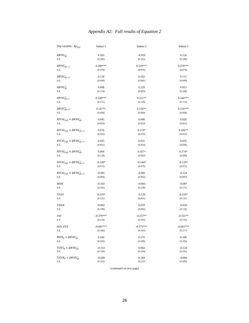
26
Appendix A2: Full results of Equation 2
Dep variable: Subset 1
Subset 2
Subset 3
0.163 -0.019 0.154
S.E. (0.180) (0.152) (0.189)
0.280*** 0.319*** 0.270***
S.E. (0.078) (0.070) (0.079)
0.118 0.102 0.115
S.E. (0.099) (0.081) (0.099)
0.098 0.129 0.053
S.E. (0.114) (0.093) (0.108)
0.338*** 0.311** 0.344***
S.E. (0.111) (0.129) (0.114)
0.147** 0.156** 0.156***
S.E. (0.058) (0.064) (0.058)
0.045 0.008 0.028
S.E. (0.059) (0.053) (0.057)
0.076 0.119* 0.106**
S.E. (0.052) (0.070) (0.053)
0.025 0.031 0.035
S.E. (0.051) (0.054) (0.049)
0.094 0.167* 0.174*
S.E. (0.118) (0.092) (0.094)
-0.128* -0.144* -0.119*
S.E. (0.073) (0.079) (0.072)
-0.091 -0.081 -0.124
S.E. (0.093) (0.092) (0.097)
-0.102 -0.093 -0.087
S.E. (0.165) (0.128) (0.171)
-0.233* -0.120 -0.219*
S.E. (0.125) (0.091) (0.131)
-0.062 0.019 -0.033
S.E. (0.109) (0.092) (0.116)
-0.379*** -0.257** -0.331**
S.E. (0.124) (0.105) (0.135)
-0.681*** -0.375*** -0.662***
S.E. (0.166) (0.143) (0.177)
0.100 0.270 0.108
S.E. (0.220) (0.180) (0.229)
-0.153 0.064 -0.124
S.E. (0.158) (0.144) (0.161)
-0.049 0.184 -0.094
S.E. (0.315) (0.222) (0.309)
(continued on next page)

27
Appendix A2: Full results of Equation 2 (continued)
Dep variable: Subset 1
Subset 2
Subset 3
0.249 0.251 0.375*
S.E. (0.199) (0.177) (0.220)
0.005 -0.013 0.005
S.E. (0.119) (0.121) (0.121)
-0.118 -0.200* -0.132
S.E. (0.142) (0.120) (0.148)
-0.201* -0.223*** -0.209*
S.E. (0.109) (0.081) (0.109)
-0.647 -0.516** -0.657
S.E. (0.497) (0.211) (0.505)
-0.126 0.015 -0.132
S.E. (0.462) (0.322) (0.491)
-0.184 -0.121 -0.153
S.E. (0.137) (0.141) (0.133)
-0.076 0.007 -0.103
S.E. (0.112) (0.142) (0.115)
-0.315 -0.220 -0.364*
S.E. (0.202) (0.194) (0.209)
0.017 0.036 0.038
S.E. (0.165) (0.120) (0.176)
-0.080 -0.023 -0.047
S.E. (0.235) (0.193) (0.244)
0.165 -0.062 0.220
S.E. (0.583) (0.334) (0.593)
0.065 -0.017 0.061
S.E. (0.105) (0.123) (0.109)
-0.136 -0.151 -0.132
S.E. (0.149) (0.154) (0.141)
0.077 0.112 0.046
S.E. (0.277) (0.215) (0.276)
-0.081*** -0.051*** -0.085***
S.E. (0.022) (0.013) (0.023)
0.057** 0.025 0.059**
S.E. (0.028) (0.017) (0.029)
-0.378*** -0.387*** -0.372***
S.E. (0.064) (0.051) (0.066)
-0.197*** -0.188*** -0.194***
S.E. (0.044) (0.033) (0.044)
0.327*** 0.232** 0.323*** S.E. (0.116) (0.091) (0.121)
Obs. 1,472 1,995 1,388
0.314 0.264 0.323
Note: Standard errors clustered at the date product level are in parentheses
(***) indicates significance at the .01 level (**) indicates significance at the .05 level (*) indicates significance at the .1 level

28
References
Aguiar, Danilo R.D., and Josana A. Santana, “Asymmetry in Farm to Retail Price Transmission: Evidence from Brazil,” Agribusiness, 18
(2002), 37-48.
Bachmeier, Lance J., and James M. Griffin, “New Evidence on Asymmetric Gasoline Price Responses,” Review of Economics and
Statistics, 85 (2003), 772-776.
Bacon, Robert W., “Rockets and Feathers: The Asymmetric Speed of Adjustment of UK Retail Gasoline Prices to Cost Changes,”
Energy Economics, 13 (1991), 211-218.
Bagwell, Kyle, and Robert W. Staiger, “Collusion over the Business Cycle,” RAND Journal of Economics, 28 (1997), 82-106.
Balmaceda, Felipe, and Paula Soruco, “Asymmetric Dynamic Pricing in a Local Gasoline Retail Market,” The Journal of Industrial
Economics, 56 (2008), 629-653.
Bénabou, Ronald, and Robert Gertner, “Search with Learning from Prices: Does Increased Inflationary Uncertainty Lead to Higher
Markups,” The Review of Economic Studies, 60 (1993), 69-93.
Borenstein, Severin, A. Colin Cameron, and Richard Gilbert, “Do Gasoline Prices Respond Asymmetrically to Crude Oil Price
Changes?,” The Quarterly Journal of Economics, 112 (1997), 305-339.
Borenstein, Severin, and Andrea Shepard, “Sticky Prices, Inventories, and Market Power in Wholesale Gasoline Markets,” The RAND
Journal of Economics, 33 (2002), 116-139.
Cabral, Luis, and Arthur Fishman, “Business as Usual: A Consumer Search Theory of Sticky Prices and Asymmetric Price Adjustment,”
International Journal of Industrial Organization, 30 (2012), 371-376.
Carlton, Dennis, “The Rigidity of Prices,” The American Economic Review, 76 (1986), 637-658.
Carlton, Dennis, “The Theory and the Facts of How Markets Clear: Is Industrial Organization Valuable for Understanding
Macroeconomics?,” in Handbook of Industrial Organization, Richard Schmalensee and Robert Willig, eds. (New York, NY: Elsevier
Science Publishers B.V., 1989).
Davidson, Carl, and Raymond Deneckere, “Long-Run Competition in Capacity, Short-Run Competition in Price, and the Cournot
Model,” The RAND Journal of Economics, 17 (1986), 404-415.
Deltas, George, “Retail Gasoline Price Dynamics and Local Market Power,” The Journal of Industrial Economics, 56 (2008), 613-628.
Duffy-Deno, Kevin, “Retail Price Asymmetries in Local Gasoline Markets,” Energy Economics, 18 (1996), 81-92.
Dutta, Shantanu, Mark Bergen, and Daniel Levy, “Price Flexibility in Channels of Distribution: Evidence from Scanner Data,” Journal
of Economic Dynamics and Control, 26 (2002a), 1845-1900.
Eckert, Andrew, “Retail Price Asymmetries in Local Gasoline Markets,” Canadian Journal of Economics, 35 (2002), 52-77.
Eckert, Andrew, “Empirical Studies of Gasoline Retailing: A Guide to the Literature,” Journal of Economic Surveys, forthcoming, 2011.
Fishman, Arthur, “Search with Learning and Price Adjustment Dynamics,” The Quarterly Journal of Economics, 11 (1996), 253-268.
Frey, Giliola, and Matteo Manera, “Econometric Models of Asymmetric Price Transmission,” Journal of Economic Surveys, 21 (2007),
349-415.
Geertz, Clifford, “The Bazaar Economy: Information and Search in Peasant Marketing,” American Economic Review, 68 (1978), 28-32.
Geweke, John, “Issues in the Rockets and Feathers Gasoline Literature,” Report to the Federal Trade Commission, 2004.
Hall, Robert L., and Charles J. Hitch, “Price Theory and Business Behavior,” Oxford Economic Papers, 2 (1939), 12-45.
Haltiwanger, John, and Joseph P. Harrington “The Impact of Cyclical Demand Movements on Collusive Pricing Behavior,” RAND
Journal of Economics, 22 (1991), 89-106.
Hannan, Timothy H., and Allen N. Berger, “The Rigidity of Prices: Evidence from the Banking Industry,” The American Economic
Review, 84 (1991), 938-945.

29
Hosken, Daniel S., Robert S. McMillan, and Christopher T. Taylor, “Retail Gasoline Pricing: What Do We Know?,” International
Journal of Industrial Organization, 26 (2008), 1425-1436.
Kahn, Charles, George Pennacchi, and Ben Sopranzetti, “Bank Consolidation and the Dynamics of Consumer Loan Interest Rates,” The
Journal of Business, 78 (2005), 99-134.
Karrenbrock, Jeffrey D., “The Behavior of Retail Gasoline Prices: Symmetric or Not?,” Federal Reserve Bank of St. Louis Review,
July/August (1991), 19-29.
Kirman, Alan, Sonia Moulet, and Rainer Schulz, “Price Discrimination and Customer Behaviour: Empirical Evidence from Marseille,”
Working Paper, 2008.
Kirman, Alan, Rainer Schulz, Wolfgang Härdle, and Axel Werwatz, “Transactions that did not Happen and their Influence on Prices,”
Journal of Economic Behavior and Organization, 56 (2005), 567-591.
Levy, Daniel, Shantanu Dutta, and Mark Bergen, “Heterogeneity in Price Rigidity: Evidence from Primary Micro Level Data,” Journal
of Money, Credit, and Banking, 34 (2002b), 197-220.
Lewis, Matthew, “Asymmetric Price Adjustment and Consumer Search: An Examination of the Retail Gasoline Market,” Journal of
Economics and Management Strategy, 20 (2011), 409-449.
Meyer, Jochen, and Stephan von Cramon-Taubadel, “Asymmetric Price Transmission: A Survey,” Journal of Agricultural Economics,
55 (2004), 581-611.
Mills, Frederick C., “The Behavior of Prices,” NBER General Series, 11 (New York: Arno Press, 1927).
Moulet, Sonia, and Juliette Rouchier, “The Influence of Seller Learning and Time Constraints on Sequential Bargaining in an Artificial
Perishable Goods Market,” Journal of Economic Dynamics & Control, 32 (2008), 2322-2348.
Neumark, David, and Steven A. Sharpe, “Market Structure and the Nature of Price Rigidity: Evidence from the Market for Consumer
Deposits,” The Quarterly Journal of Economics, 107 (1992), 657-680.
Noel, Michael D., “Edgeworth Price Cycles, Cost-Based Pricing and Sticky Pricing in Retail Gasoline Markets,” The Review of
Economics and Statistics, 89 (2007), 324-334.
Peltzman, Sam, “Prices Rise Faster Than They Fall,” Journal of Political Economy, 108 (2000), 466-502.
Rotemberg, Julio J., and Garth Saloner, “A Supergame-Theoretic Model of Price Wars during Booms,” The American Economic Review,
76 (1986), 390-407.
Sherman, Joshua, and Avi Weiss, “An Empirical Analysis of Search Costs and Price Dispersion,” Working Paper, 2012.
Shy, Oz, Industrial Organization: Theory and Applications. (Cambridge, MA: The MIT Press, 1996).
Shy, Oz, “A Quick-and-Easy Method for Estimating Switching Costs,” International Journal of Industrial Organization, 20 (2002), 71-
87.
Sweezy, Paul, “Demand under Conditions of Oligopoly,” Journal of Political Economy, 47 (1939), 568-573.
Tappata, Mariano, “Rockets and Feathers: Understanding Asymmetric Pricing,” RAND Journal of Economics, 40 (2009), 673-687.
Tirole, Jean, The Theory of Industrial Organization. (Cambridge, MA: MIT Press, 1988).
Verlinda, Jeremy A., “Do Rockets Rise Faster and Feathers Fall Slower in an Atmosphere of Local Market Power? Evidence from the
Retail Gasoline Market,” The Journal of Industrial Economics, 56 (2008), 581-612.
Ward, Ronald W., “Asymmetry in Retail, Wholesale and Shipping Point Pricing for Fresh Vegetables,” American Journal of Agricultural
Economics, 62 (1982), 205-212.
Wolman, Alexander L., “The Frequency and Costs of Individual Price Adjustment,” Managerial and Decision Economics, 28 (2007),
531-552.
Yang, Huanxing, and Lixin Ye, “Search with Learning: Understanding Asymmetric Price Adjustments,” RAND Journal of Economics, 39
(2008), 547-564.

30
Table 1: Consumers’ ex-ante expected rival price
Condition
1
1
2A
2A
2A
2B
Table 2: Period of retail price response to a change in cost
Cost increase in
period
Cost decrease in period
,
Rival firms
Isolated firms
(pooling equilibrium)
Isolated firms
(separating equilibrium)
Table 3: Total number of observations collected and number of firms per area
Observations of a firm selling
(including firms posting price)
Observations of a firm
posting price
Observations 11,983 7,491
Area date product combinations 3,107 2,474
Number of firms per
area date product combination:
Average 3.857 3.028
Standard deviation 2.2 2.083
Min 1 1
Max 11 11

31
Table 4: Percentage of observations in which a firm faces at least one rival:
Two consecutive price change lags, firm status unchanged during same time period (n = 2,788)
Product / Area A B C D Overall
Beet 0% 6% 0% 0% 4%
Cauliflower 0% 0% 0%
Corn 100% 27% 0% 45%
Cucumber 52% 52% 41% 40% 48%
Kohlrabi 0% 11% 0% 0% 7%
Red Cabbage 0% 0% 0% 0%
Red Pepper 51% 18% 90% 0% 41%
Sweet Potato 35% 11% 0% 0% 11%
White Cabbage 0% 0% 13% 7% 6%
Yellow Pepper 0% 7% 19% 0% 8%
Note: A cell indicating 0% indicates that observations for isolated firms exist. A blank cell indicates that no observations exist for either firm type.

32
Table 5: OLS price level regression (shekels per kilogram)
Dep variable: Subset 1
Subset 2
Subset 3
-0.262***
-0.215***
-0.286***
S.E. (0.044)
(0.043)
(0.045)
0.417***
0.351***
0.399***
S.E. (0.060)
(0.048)
(0.063)
0.100
0.069
0.096
S.E. (0.141)
(0.125)
(0.147)
0.031
0.011
0.032
S.E. (0.148)
(0.125)
(0.153)
-0.009
0.015
0.012
S.E. (0.133)
(0.123)
(0.141)
-0.253**
-0.214*
-0.214*
S.E. (0.120)
(0.114)
(0.127)
-0.253
-0.056
-0.238
S.E. (0.212)
(0.194)
(0.219)
0.978***
0.659***
0.982***
S.E. (0.092)
(0.084)
(0.092)
-0.340***
-1.011***
-0.334***
S.E. (0.091)
(0.124)
(0.092)
-0.833***
-1.508***
-0.817***
S.E. (0.089)
(0.105)
(0.090)
1.456***
S.E. (0.286)
0.511***
0.971***
0.507***
S.E. (0.183)
(0.157)
(0.185)
0.996***
S.E. (0.169)
0.135
0.296
0.205
S.E. (0.232)
(0.204)
(0.239)
3.029***
2.555***
3.095***
S.E. (0.355)
(0.199)
(0.361)
-0.546**
S.E. (0.269)
-0.247
S.E. (0.204)
Constant 3.044***
3.503***
3.083***
S.E. (0.180)
(0.162)
(0.186)
Obs. 1,472
1,995
1,388
0.647
0.591
0.643
Note: Standard errors clustered at the date product level are in parentheses. During the data collection period in 2009, on average
6.33 shekels = £1.00.
(***) indicates significance at the .01 level (**) indicates significance at the .05 level (*) indicates significance at the .1 level

33
Table 6: Legend for Tables 7, 8, and 9A – 9D
Isolated firm Interpretation
Isolated firm price response in period t to a decrease in wholesale price in period t
Isolated firm price response in period t to an increase in wholesale price in period t
Isolated firm price response in period t+1 to a decrease in wholesale price in period t
Isolated firm price response in period t+1 to an increase in wholesale price in period t
Isolated firm price response in period t+2 to a decrease in wholesale price in period t
Isolated firm price response in period t+2 to an increase in wholesale price in period t
Rival firm Interpretation
Rival firm price response in period t to a decrease in wholesale price in period t
Rival firm price response in period t to an increase in wholesale price in period t
Rival firm price response in period t+1 to a decrease in wholesale price in period t
Rival firm price response in period t+1 to an increase in wholesale price in period t
Rival firm price response in period t+2 to a decrease in wholesale price in period t
Rival firm price response in period t+2 to an increase in wholesale price in period t

34
Table 7: Predictions of the theoretical model when isolated firms pool57
(calculation using coefficients estimated from Equation 2 in parentheses)
Morning of wholesale price change
Isolated firm Mon Tues Wed Thur
Sum of coefficients obtained from Equation 2
Sum of coefficients obtained from Equation 2
Sum of coefficients obtained from Equation 2
Sum of coefficients obtained from Equation 2
Sum of coefficients obtained from Equation 2
Sum of coefficients obtained from Equation 2
Rival firm Mon Tues Wed Thur
Sum of coefficients obtained from Equation 2
Sum of coefficients obtained from Equation 2
Sum of coefficients obtained from Equation 2
Sum of coefficients obtained from Equation 2
Sum of coefficients obtained from Equation 2
Sum of coefficients obtained from Equation 2
57 A checkmark indicates a prediction of a retail price response to a wholesale price change (in the same direction) for a given period.

35
Table 8: Retail price response to a one shekel per kilogram change in wholesale price
(calculated using coefficient estimates obtained from Equation 2)
Subset 1
Subset 2
Subset 3
Morning of wholesale price change
Morning of wholesale price change
Morning of wholesale price change
Isolated firm Mon Tues Wed Thur
Mon Tues Wed Thur
Mon Tues Wed Thur
0.262** 0.010 0.163 0.113
0.251*** 0.045 -0.019 0.164
0.262** 0.030 0.154 0.061
-value (0.011) (0.905) (0.367) (0.697)
(0.007) (0.413) (0.900) (0.377)
(0.013) (0.726) (0.415) (0.831)
0.348** 0.103 0.098 -0.020
0.380*** 0.115 0.129 -0.071
0.428*** 0.058 0.053 -0.079
-value (0.010) (0.304) (0.388) (0.897)
(0.004) (0.199) (0.170) (0.485)
(0.007) (0.511) (0.622) (0.589)
0.079 0.280*** -0.367 0.154
0.096 0.319*** -0.196 0.335
0.061 0.270*** -0.387 0.138
-value (0.227) (0.000) (0.481) (0.731)
(0.135) (0.000) (0.326) (0.282)
(0.331) (0.001) (0.467) (0.772)
0.154* 0.338*** 0.262*** 0.023
0.189*** 0.311** 0.318*** 0.091
0.190** 0.344*** 0.241*** -0.020
-value (0.095) (0.003) (0.000) (0.887)
(0.005) (0.016) (0.001) (0.505)
(0.028) (0.003) (0.001) (0.905)
0.118 0.136 0.039 0.284
0.102 0.138* 0.079 0.040
0.115 0.153 0.067 0.335
-value (0.233) (0.289) (0.854) (0.619)
(0.210) (0.096) (0.646) (0.901)
(0.247) (0.262) (0.758) (0.564)
0.147** 0.211** 0.011 0.223
0.156** 0.139 0.005 0.268
0.156*** 0.218* 0.024 0.202
-value (0.012) (0.049) (0.928) (0.434)
(0.016) (0.236) (0.969) (0.199)
(0.008) (0.056) (0.817) (0.478)
Rival firm Mon Tues Wed Thur
Mon Tues Wed Thur
Mon Tues Wed Thur
0.308** 0.055 0.208 0.159
0.259** 0.054 -0.011 0.173
0.290** 0.058 0.182 0.089
-value (0.034) (0.435) (0.243) (0.589)
(0.042) (0.284) (0.944) (0.370)
(0.048) (0.439) (0.330) (0.759)
0.441** 0.197* 0.192** 0.074
0.547*** 0.283** 0.296*** 0.097
0.602*** 0.233** 0.227** 0.095
-value (0.041) (0.069) (0.026) (0.523)
(0.005) (0.012) (0.002) (0.295)
(0.009) (0.022) (0.010) (0.427)
0.155** 0.355*** -0.291 0.230
0.215*** 0.438*** -0.077 0.453
0.166** 0.375*** -0.281 0.244
-value (0.036) (0.000) (0.582) (0.621)
(0.005) (0.000) (0.726) (0.174)
(0.026) (0.000) (0.603) (0.622)
0.026 0.210* 0.134** -0.105
0.045 0.167 0.173** -0.053
0.071 0.225** 0.122** -0.139
-value (0.820) (0.059) (0.022) (0.582)
(0.638) (0.214) (0.010) (0.750)
(0.499) (0.048) (0.038) (0.478)
0.143 0.161 0.064 0.309
0.133 0.170 0.110 0.071
0.150 0.187 0.102 0.370
-value (0.137) (0.237) (0.759) (0.590)
(0.126) (0.114) (0.515) (0.828)
(0.131) (0.210) (0.634) (0.526)
0.055 0.120 -0.081 0.132
0.075 0.058 -0.076 0.187
0.032 0.094 -0.100 0.078
-value (0.444) (0.269) (0.658) (0.650)
(0.399) (0.613) (0.687) (0.421)
(0.665) (0.408) (0.577) (0.785)
Note: The -values associated with standard errors clustered at the date product level are in parentheses.
(***) indicates significance at the .01 level (**) indicates significance at the .05 level (*) indicates significance at the .1 level

36
Tables 9A-9B: Robustness checks of Equation 2 (Subset 3)
9A: With interactions
9B: Without error correction terms
Morning of wholesale price change
Morning of wholesale price change
Isolated firm Mon Tues Wed Thur
Mon Tues Wed Thur
0.211 0.062 -0.011 -0.141 0.242** 0.023 0.034 0.070
-value (0.280) (0.516) (0.953) (0.435) (0.024) (0.707) (0.865) (0.764)
0.472*** 0.007 0.087 -0.057 0.440*** 0.017 0.021 -0.054
-value (0.000) (0.948) (0.456) (0.669) (0.004) (0.848) (0.852) (0.662)
0.062 0.251*** -0.118 -0.119 0.105 0.354*** -0.411 0.209
-value (0.297) (0.025) (0.684) (0.612) (0.134) (0.000) (0.469) (0.647)
0.169** 0.315*** 0.288*** -0.011 0.246*** 0.340*** 0.264*** 0.070
-value (0.028) (0.008) (0.000) (0.939) (0.003) (0.007) (0.001) (0.683)
0.095 0.200** 0.387** 0.726 0.145 0.153 0.062 0.273
-value (0.300) (0.050) (0.048) (0.158) (0.148) (0.276) (0.779) (0.634)
0.081 0.146 0.048 0.104 0.165** 0.247** 0.055 0.325
-value (0.066) (0.110) (0.280) (0.693) (0.015) (0.014) (0.634) (0.234)
Rival firm Mon Tues Wed Thur Mon Tues Wed Thur
0.314** 0.044 0.284 0.282 0.253* 0.034 0.045 0.080
-value (0.047) (0.554) (0.270) (0.516) (0.087) (0.462) (0.823) (0.736)
0.552 0.289** 0.202*** 0.074 0.636*** 0.213** 0.217** 0.142
-value (0.154) (0.028) (0.007) (0.539) (0.005) (0.030) (0.017) (0.159)
0.164** 0.404*** -0.441 0.430 0.199** 0.448*** -0.317 0.303
-value (0.028) (0.007) (0.502) (0.556) (0.017) (0.000) (0.582) (0.523)
0.125 0.247** 0.083 -0.141 0.138 0.232* 0.155*** -0.038
-value (0.332) (0.033) (0.276) (0.534) (0.158) (0.058) (0.002) (0.850)
0.168 0.168 -0.098 0.216 0.170* 0.178 0.086 0.298
-value (0.110) (0.330) (0.725) (0.751) (0.090) (0.240) (0.687) (0.605)
0.109* 0.176 -0.134 0.142 0.050 0.132 -0.060 0.210
-value (0.093) (0.178) (0.611) (0.642) (0.499) (0.182) (0.759) (0.449)
Note: The -values associated with standard errors clustered at the date product level are in parentheses.
(***) indicates significance at the .01 level (**) indicates significance at the .05 level (*) indicates significance at the .1 level
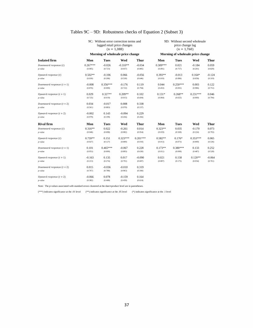
37
Tables 9C – 9D: Robustness checks of Equation 2 (Subset 3)
9C: Without error correction terms and
lagged retail price changes
9D: Without second wholesale
price change lag
Morning of wholesale price change
Morning of wholesale price change
Isolated firm Mon Tues Wed Thur
Mon Tues Wed Thur
0.267*** -0.026 -0.310** -0.034 0.309*** 0.021 -0.184 0.059
-value (0.005) (0.723) (0.037) (0.885) (0.001) (0.757) (0.201) (0.829)
0.502** -0.106 0.066 -0.056 0.393** -0.013 0.164* -0.124
-value (0.030) (0.206) (0.530) (0.646) (0.019) (0.896) (0.058) (0.319)
-0.008 0.356*** -0.176 0.119 0.044 0.250*** 0.003 0.122
-value (0.876) (0.000) (0.722) (0.794) (0.453) (0.001) (0.986) (0.751)
0.029 0.327** 0.209** 0.102 0.131* 0.268** 0.231*** 0.046
-value (0.725) (0.010) (0.015) (0.604) (0.064) (0.025) (0.000) (0.794)
0.034 -0.017 0.008 0.338
-value (0.561) (0.883) (0.970) (0.537)
-0.002 0.143 -0.094 0.229
-value (0.979) (0.199) (0.456) (0.456)
Rival firm Mon Tues Wed Thur Mon Tues Wed Thur
0.316** 0.022 -0.261 0.014 0.323** 0.035 -0.170 0.073
-value (0.046) (0.698) (0.082) (0.954) (0.019) (0.569) (0.224) (0.793)
0.759** 0.151 0.323*** 0.201*** 0.582** 0.176* 0.353*** 0.065
-value (0.027) (0.127) (0.000) (0.010) (0.013) (0.073) (0.000) (0.536)
0.101 0.465*** -0.067 0.228 0.173** 0.380*** 0.133 0.252
-value (0.053) (0.000) (0.893) (0.630) (0.011) (0.000) (0.487) (0.528)
-0.163 0.135 0.017 -0.090 0.021 0.158 0.120** -0.064
-value (0.213) (0.274) (0.791) (0.687) (0.807) (0.175) (0.034) (0.761)
0.015 -0.036 -0.010 0.319
-value (0.767) (0.788) (0.963) (0.560)
-0.066 0.078 -0.159 0.164
-value (0.382) (0.468) (0.459) (0.624)
Note: The -values associated with standard errors clustered at the date product level are in parentheses.
(***) indicates significance at the .01 level (**) indicates significance at the .05 level (*) indicates significance at the .1 level

38
Table 10: Number of observations by weekday, number of lags, direction of wholesale price,
and firm type (Subset 3)
No wholesale price change
Wholesale price decrease
Wholesale price increase
Observations
Observations
Observations
Morning of wholesale price change Isolated Rival Date products
Isolated Rival Date products
Isolated Rival Date products
Monday
First period retail price response (t) 12 27 8
88 108 19
17 20 6
Second period retail price response (t+1) 10 21 6
91 123 23
18 23 6
Third period retail price response (t+2) 10 18 7
95 131 23
11 17 6
Tuesday
First period retail price response (t) 31 41 7
46 62 13
41 60 13
Second period retail price response (t+1) 27 37 7
40 55 13
47 71 14
Third period retail price response (t+2) 19 30 8
44 67 15
47 64 12
Wednesday
First period retail price response (t) 24 36 7
17 28 8
59 81 14
Second period retail price response (t+1) 23 38 9
23 29 8
57 82 15
Third period retail price response (t+2) 27 44 10
34 42 12
62 77 13
Thursday
First period retail price response (t) 11 26 8
34 45 11
59 85 17
Second period retail price response (t+1) 13 25 6
39 53 13
67 89 18
Third period retail price response (t+2) 16 25 6
32 49 10
58 73 16

39
Table 11: Three-day cumulative response to a one shekel per kilogram change in wholesale price
Subset 1
Subset 2
Subset 3
Morning of wholesale price change
Morning of wholesale price change
Morning of wholesale price change
Mon Tues Wed Thur
Mon Tues Wed Thur
Mon Tues Wed Thur
Isolated firm downward response 0.460*** 0.425*** -0.166 0.552
0.449*** 0.503*** -0.137 0.539
0.437*** 0.453*** -0.165 0.534
Isolated firm upward response 0.649*** 0.652*** 0.371** 0.227
0.725*** 0.565*** 0.451*** 0.288
0.775*** 0.620*** 0.318** 0.103
Rival firm downward response 0.606*** 0.571*** -0.020 0.697
0.608*** 0.662*** 0.022 0.697
0.606*** 0.621*** 0.003 0.702
Rival firm upward response 0.523** 0.527*** 0.246 0.101
0.667*** 0.507** 0.393* 0.230
0.706** 0.551*** 0.249 0.034
Note: Tests of significance correspond to the null hypothesis that the cumulative three-day response to a wholesale price change in Equation 2 is zero. Significance is associated with standard errors clustered at
the date product level.
(***) indicates significance at the .01 level (**) indicates significance at the .05 level (*) indicates significance at the .1 level
Table 12A: Predictions of tests of cumulative response equality
Predictions
Morning of wholesale price change
Null hypothesis Mon Tues Wed Thur
: Cumulative down isolated = cumulative down rival Not equal (isolated < rival)
: Cumulative up isolated = cumulative up rival Not equal (isolated < rival)
: Cumulative down isolated = cumulative up isolated Equal Equal Equal Equal
: Cumulative down rival = cumulative up rival Equal Equal Equal Equal
Table 12B: Results of cumulative response equality tests
The -values associated with rejecting the null hypothesis
Subset 1
Subset 2
Subset 3
Morning of wholesale price change
Morning of wholesale price change
Morning of wholesale price change
Null hypothesis Mon Tues Wed Thur
Mon Tues Wed Thur
Mon Tues Wed Thur
0.090*
0.098*
0.047**
0.389
0.693
0.617
0.501 0.395 0.412 0.738
0.275 0.807 0.130 0.675
0.257 0.545 0.471 0.669
0.811 0.864 0.686 0.542
0.852 0.529 0.367 0.455
0.782 0.798 0.714 0.512
Note: The -values are associated with standard errors clustered at the date product level.
(**) indicates significance at the .05 level (*) indicates significance at the .1 level

40
Point A Point B
Isolated Firm N>1 Rival Firms
Exogenous location of consumers
(i.e., residence, place of employment)
Exogenous location of consumers
(i.e., residence, place of employment)
Figure 1A: The isolated firm and the rival firms
Isolated Firm Isolated Firm
N>1 Rival Firms Point B
Point A Point C
Figure 1B: One of several possible alternate renderings of the theoretical setting
Exogenous location of consumers
(i.e., residence, place of employment)
Exogenous location of consumers
(i.e., residence, place of employment)
Exogenous location of consumers
(i.e., residence, place of employment)

41
Figure 2: Map of Mahane Yehuda58
58 We thank Shmuel Browns for providing us with this hand-drawn map. We have added notation to indicate the locations of Areas A-D, the bus lines, and additional parking lots.
Area A
Area B
Area D
Area C
Parking Lot
Buses run along
Jaffa Road
Parking Lot

42
Figures 3A – 3J: Wholesale price and average retail price by product
(Shekels per kilogram (Y axis), daily, April 2 – August 4, 2009 (X axis))
Note: Not including Sundays. As noted in the text, the wholesale price is the daily common price recorded at the Jerusalem wholesale market for a given product. The average retail price is the
daily average of all posted prices for a given product. One cauliflower observation of 14 shekels per kilogram on July 15, 2009 is not shown. An absence of observations in the average retail
price series for cauliflower and red cabbage indicates that there were no posted prices for that particular product during the time period. For seasonality purposes corn enters the data series 11
periods after the beginning of the data set.
0
2
4
6
8
10
3A: Beets
Average Retail Price Wholesale Price
0
2
4
6
8
10
3B: Cauliflower
Average Retail Price Wholesale Price
0
2
4
6
8
10
3C: Corn
Average Retail Price Wholesale Price
0
2
4
6
8
10
3D: Cucumbers
Average Retail Price Wholesale Price
0
2
4
6
8
10
3E: Kohlrabi
Average Retail Price Wholesale Price
0
2
4
6
8
10
3F: Red Cabbage
Average Retail Price Wholesale Price
0
2
4
6
8
10
3G: Red Peppers
Average Retail Price Wholesale Price
0
2
4
6
8
10
3H: Sweet Potatoes
Average Retail Price Wholesale Price
0
2
4
6
8
10
3I: White Cabbage
Average Retail Price Wholesale Price
0
2
4
6
8
10
3J: Yellow Peppers
Average Retail Price Wholesale Price