Price Dispersion and the Border E↵ect⇤

Ryan ChahrourBoston College

Luminita StevensUniversity of Maryland

September 2019

Abstract

Cross-country price di↵erences could reflect regional market segmentation withincountries or national segmentation at the border. In a search-based model of pricesetting, identifying national versus regional segmentation requires data on regionaltrade flows. A calibration to U.S. and Canadian data implies predominantly re-gional frictions: U.S. producers are three times more likely to sell in their homeregion than another U.S. region and Canadian producers are seven times morelikely to sell in their home region than another Canadian region. Frictions vis-a-visforeign regions are only slightly higher. Models that ignore regional segmentationcan misstate the severity of frictions at the border.

Keywords: Law of one price, Real exchange rates, Trade barriers, Home bias

JEL Codes: F41, F30, E30

⇤We would like to thank Emi Nakamura, Jaromir Nosal, John Shea, Jon Steinsson, Rosen Valchev,and seminar participants at the Federal Reserve Bank of Boston, Boston College, and Columbia Univer-sity for very helpful comments. We are grateful to Joao Ayres for excellent research assistance. Contact:ryan.chahrour@bc.edu and stevens@econ.umd.edu.

1 Introduction

A large literature in international macroeconomics measures the frictions that hin-

der the arbitrage of price di↵erences across countries. The seminal paper of Engel and

Rogers (1996) documented significant border frictions using semi-aggregated price in-

dices for goods sold in the United States and Canada. Subsequent work has sought to

refine these estimates using increasingly disaggregated data. Empirical work by Gopinath

et al. (2011), Burstein and Jaimovich (2012), Broda and Weinstein (2008), and Crucini

and Telmer (2012) has shown that product-level price di↵erences across countries are

consistent with a very large degree of segmentation at the national border. Following

Gorodnichenko and Tesar’s (2009) criticism of reduced-form treatment of cross-border

relative price data, and their call for a more structural approach, the empirical evidence

has been complemented by structural work reinforcing the conclusion that high cross-

country segmentation is crucial for generating realistic good-level violations of the law of

one price.

We demonstrate an identification problem—even within structural frameworks—in

disentangling segmentation that is induced by national borders from the segmentation

that exists between regions or markets within a country. Using a two-country multi-

region model of trade, we show that cross-country price and trade data are not su�cient

for determining if international price dispersion arises from a friction inhibiting trade

across countries or from a friction that inhibits trade across regions internally. We also

show that adding data on regional trade patterns is precisely what is needed to separately

identify the parameters governing within-country and across-country trade frictions, and

we estimate these two levels of segmentation for the United States and Canada.

1

Our central finding is that much of the measured market segmentation occurs at the

subnational regional level. To arrive at this result, we calibrate our model to match a set

of facts regarding good-level violations of the law of one price across the United States–

Canada border, as well as both international and internal levels of trade for the two

countries. Matching both sets of facts simultaneously requires a calibration in which re-

gional markets are strongly segmented and the national border generates little additional

segmentation.

We obtain our results using a search-based model of international trade in which

retailers engage in costly sequential search for the best price among the producers that are

active in the retailers’ local markets. The search friction, combined with a distribution

of producer-specific productivity shocks, gives rise to endogenous price dispersion in

equilibrium. Generating significant price dispersion at the local level is relevant for

measuring the severity of international border frictions because, as demonstrated by

Gorodnichenko and Tesar (2009), the existence of price dispersion within countries can

bias estimates of the “size” of the border.

The model allows for heterogeneous segmentation across regions, with the mass of

producers that are headquartered in one region and active in another depending on both

market sizes and on a pure market bias parameter. This specification enables us to

quantify the degree of domestic and international segmentation for each country, while

taking into account di↵erential trade patterns that reflect market size di↵erences. The

model nests regionally and nationally segmented markets. Under regional segmentation,

producers headquartered in one region are less likely to set up shop in other regions,

while under national segmentation, producers are equally likely to set up shop in the

2

regions within their own country, but less likely to set up shop in the other country. We

use price and trade flows data to estimate the size of these relative biases.

Applied to United States and Canada data, our model implies that the apparent

segmentation at the national border is primarily a reflection of regional segmentation.

Splitting the United States in two equal-sized regions, we estimate that on average pro-

ducers are 3 times more likely to sell to retailers in their own region than to retailers in

the “away” U.S. region. Hence, there are significant barriers to the flow of goods across

U.S. regions. Crossing the national border further reduces access, but this barrier is less

severe than the regional barrier, with American producers only 23% more likely to sell

in the “away” domestic region than to a Canadian region.

Furthermore, we uncover substantial asymmetry across countries in the severity of

these frictions. Canadian producers are 7 times more likely to sell in their own region

than in the “away” Canadian region, and 11 times more likely to sell in their own region

than in an American region. Overall, regional bias is a major component of the national

home bias, and it appears more severe for Canadian producers.

Our measures of relative bias provide a simple way to parameterize all the frictions

and barriers to trade, either bilateral or unilateral, which may a↵ect the likelihood of

transacting across regions. These include informational advantages that ease access to

the chain of production in one’s own market, and external barriers that make transacting

with firms located outside one’s own network more di�cult. Together with the size of

each market, the segmentation parameters determine how producers are matched with

the retailers of di↵erent regions, which pins down the distribution of prices available in

each region. The model generates pricing to market, as producers charge di↵erent prices

3

in di↵erent regions, depending on local demand conditions and competitive pressures. In

turn, pricing to market contributes to cross-border price di↵erentials, consistent with the

empirical evidence emphasized by Burstein and Gopinath (2014).

Our paper relates to an extensive literature examining violations of the law of one

price, recently surveyed by Burstein and Gopinath (2014). Alessandria (2004, 2009) and

Alessandria and Kaboski (2011) also use a search friction to motivate cross-border price

di↵erences, although these papers do not emphasize the distinction between frictions

that occur across markets within countries versus those that occur at the border. Other

search models of the product market that focus on price dispersion across stores in a

single market include Kaplan and Menzio (2015) and Menzio and Trachter (2015, 2018).

Our approach resembles that of Gopinath et al. (2011) and Burstein and Jaimovich

(2012) in that we consider a model with a real friction in goods markets, coupled with

country heterogeneity in the distribution of firm costs. Burstein and Jaimovich (2012)

model within-country regions and point out an identification problem using prices alone

to distinguish between di↵erences in demand-shock correlations and di↵erences in markup

elasticities across markets. However, the forces they discuss map to within-region price

dispersion in our economy.1 We assume perfect correlation of demand conditions within

countries, but show there is nevertheless an identification problem regarding the level

at which markets are segmented. Other related papers using product-level price data

include Baxter and Landry (2017), Goldberg and Hellerstein (2013), Fitzgerald and Haller

(2014), and De Loecker et al. (2016). Alternative structural frameworks are considered

by Atkeson and Burstein (2008), Drozd and Nosal (2012) and Candian (2019).

1Prices are dispersed within regions in our economy, but not in Burstein and Jaimovich (2012).

4

Methodologically, our paper is distinct from the earlier literature because it incorpo-

rates price and quantity data simultaneously. An exception is Boivin et al. (2012), who

undertake a nonstructural analysis using price and quantity data from a retailer in the

online book market, and find substantial international market segmentation.

Our results are also related to gravity models of trade. McCallum (1995) finds that

large border frictions are required to account for within- versus across-country trades

levels between the United States and Canada. Anderson and van Wincoop (2003) show

that the estimated border e↵ect on trade is much smaller once theoretically motivated

measures of multilateral resistance are added to the estimation. Wolf (2000) and Millimet

and Osang (2007) focus on intranational trade barriers. Other papers in this area include

Chen (2004), Hillberry and Hummels (2008), and Atkin and Donaldson (2015).

2 Model

We develop a multi-region, multi-sector two-country model in which search frictions

generate price dispersion both within and across regions. We model the search friction as

in Reinganum (1979), whose model of homogeneous buyers and heterogeneous sellers we

develop into a general equilibrium framework with producers, retailers and consumers.

We then extend the model to a two-country world with two regions in each country,

featuring producers selling the same good to retailers in multiple regions.

2.1 Single-Region Economy

The economy features a representative consumer, a perfectly competitive nontradable

sector, and a monopolistically competitive tradable goods sector. We focus on the trad-

able goods sector since the puzzle is that the law of one price also fails to hold for traded

5

goods, for which arbitrage should—but does not—eliminate price di↵erences.

Consumers: The representative consumer buys goods in sectors N and T (which rep-

resent nontradables and tradables in the two-country model) and supplies labor to solve

maxCT ,CN ,L

log⇣C�

TC1��N

⌘� L1+1/

1 + 1/ (1)

PTCT + PNCN WL+ ⇧, (2)

where CN and CT denote aggregate consumption in the two sectors, PN and PT are

the respective price indices, L is labor supply, W the economy-wide nominal wage, and

⇧ nominal firm profits. The parameter � 2 (0, 1) governs the share of sector T in

consumption, and > 0 is the Frisch elasticity of labor supply. Consumer optimization

implies that expenditure is allocated across the two sectors according to PTCT/PNCN =

�/(1� �), and labor supply is given by L1/ = �W/ PTCT .

Sector T is monopolistically competitive, with a continuum of goods indexed by i and

a continuum of varieties ⌫ for each good. At each level, consumption is aggregated using

CT =

✓Z 1

0

c"�1"

i di

◆ ""�1

and ci =

✓Z 1

0

c⌘i�1⌘i

i⌫ d⌫

◆ ⌘i⌘i�1

, (3)

where " > 1 is the elasticity of substitution across goods and ⌘i > 0 is the elasticity of

substitution across varieties of good i. The price indices are PT ⌘⇣R 1

0 p1�"i di⌘ 1

1�"and

pi ⌘⇣R 1

0 p1�⌘ii⌫ d⌫⌘ 1

1�⌘i . Demand at the good and variety level are given by

ci = p�"i P "TCT and ci⌫ = p�⌘ii⌫ p⌘ii ci. (4)

Sector N is competitive, with a homogeneous good produced by a representative firm.

6

Retailers: A unit mass of multi-product retailers indexed by ⌫ search for goods on

behalf of consumers. Retailers know the distribution of prices posted by the producers

(or distributors) of each good, but they do not know which producer sells at what price.

Instead, they pay a fixed search cost to sample from the distribution of producer prices.

Upon meeting a producer, each retailer either purchases its entire demand at the sampled

price, or pays the search cost again to meet a new producer. Search continues until

each retailer has settled on a single supplier for each good. Retailers then costlessly

di↵erentiate each good i into a retailer-specific variety, which they sell to consumers.

Placing the search friction at the retailer level is motivated by the evidence that retail

markups do not vary much with nominal exchange rates (Goldberg and Hellerstein, 2008;

Gopinath et al., 2011), that retail-level price changes follow changes in wholesale costs

(Goldberg and Hellerstein, 2013; Eichenbaum et al., 2011), and that overall “distribution

wedges” are stable over time (Berger et al., 2012). We abstract from the local cost

component by assuming that retailers costlessly di↵erentiate goods because prior work

has found that such costs are also insensitive to exchange rate movements.

Each retailer maximizes total per-period profits across all the goods it sells,

⇡R⌫ =

Z 1

0

⇡r (pi⌫ , bpi⌫) di, (5)

⇡r (pi⌫ , bpi⌫) = (pi⌫ � bpi⌫) ci⌫ � ni⌫ , (6)

where bpi⌫ is the producer price upon which retailer ⌫ settles after completing the search

for good i in the period, ci⌫ is demand given by (4), > 0 is the fixed search cost, and

ni⌫ is the number of times the retailer searches for a potential supplier of good i. Since

di↵erentiation at the retail level is costless, the retailer charges a constant markup over

7

the producer price, pi⌫ = µibpi⌫ , with µi ⌘ ⌘i/ (⌘i � 1).

The search process is independent across goods (since we assume that there are di↵er-

ent suppliers for di↵erent goods) and each retailer’s variety competes with the varieties

of the same good from other retailers. As a result, the retailer maximizes profits good by

good. The sequential nature of search implies that a retailer’s choice to continue looking

for a better price is independent of the number of producers already sampled. Given the

currently sampled price bpi⌫ and the distribution fi of producer prices available to the

retailer, the retailer’s search decision maximizes the value function

V (bpi⌫ ; fi) = max{V s(fi), Vns(bpi⌫)}, (7)

where V s(fi) is the value of continuing to search, which integrates over the distribution

of possible producer prices, and V ns(bpi⌫) is the value of halting the search, which yields

the maximum value at the currently sampled price:

V s(fi) =

ZV (bp; fi)fi(bp)dbp� , (8)

V ns(bpi⌫) = maxp⇡r (p, bpi⌫) . (9)

The optimal search strategy is a stopping rule defined by a unique reservation price

ri for each good that equates the value of searching to that of stopping the search. All

retailers sampling a price less than or equal to this threshold stop searching and purchase

all their demand for good i at the sampled price, and all retailers sampling a price above

it continue to search for a better o↵er.

Producers: For each good i, there is a unit mass of potential producers j characterized

by the production function yij = Aijhij, where Aij is idiosyncratic productivity and hij is

8

the labor input. Each producer potentially sells to multiple retailers. Since the producer

does not engage in price discrimination among the retailers in a given market and since

retailers are symmetric, each retailer who settles on a given producer demands the same

quantity. Letting �ij denote the mass of retailers who settle on producer j (determined

in equilibrium), a producer setting price bpi,j faces total demand

xij =

8>>><

>>>:

�ijbp�⌘iij bp⌘ii ci if bpij ri

0 if bpij > ri.

(10)

The producer maximizes profits given by (bpij �W/Aij)xij, where W is the aggregate

wage. The optimal price is then a constant markup over marginal cost, up to the retailers’

reservation price, bpij = min {µiW/Aij, ri} , where µi is the good-level markup. Since

search is undirected, the producer cannot use price to a↵ect the mass of customers, so

�ij = �i is the same across all producers j. However, since demand is elastic, lower-cost

producers set prices below the reservation price to capture more demand per customer.

Search Equilibrium: An equilibrium in the producer-retailer market for good i is a

retail reservation price ri and a distribution of producer prices fi such that (a) given

fi, retailers choose the optimal stopping rule governed by ri and (b) given ri, producers

maximizing profits generate fi. There is no search in equilibrium, since all producers

either post prices that are weakly below this reservation price or shut down.

Let the cumulative distribution of marginal costs across producers of good i be de-

9

noted by Gi. The resulting cumulative distribution of producer prices is given by

Fi(bp) =

8>>><

>>>:

Gi

⇣bpµi

⌘if bp ri

1 if bp > ri

. (11)

Since there is a unit mass of retailers and a unit mass of potential producers, the mass

of retailers per active producer of each good i is then given by �i = 1/(1�Gi(ri)).

In models of search with homogeneous goods, arbitrarily small search costs can re-

sult in a collapse of the price distribution at the monopoly price—the Diamond (1971)

paradox. In our setup, heterogeneous production costs and elastic demand generate a

non-degenerate distribution of prices, as shown by Reinganum (1979) for a single prod-

uct with many buyers and sellers. The degree of dispersion in prices depends on the

cross-sectional dispersion of producer costs, and the out-of-equilibrium threat of search

leads to incomplete pass-through of marginal cost for high-cost producers: markups are

constant for all producers with marginal costs less than ri/µi, and are decreasing for

active producers with costs above this threshold.2

2.2 Multi-Region Economy

We now consider two countries, United States and Canada, each with two regions.

The countries di↵er along several dimensions: size, severity of trade and search frictions,

the realization of aggregate and good-specific shocks, and the distribution of idiosyn-

cratic productivity shocks. These asymmetries give rise to pricing-to-market, where a

given producer charges di↵erent prices to retailers located in di↵erent regions. To reduce

notation, we drop the product subscript i wherever there is no confusion.

2Other ways to break the Diamond paradox are heterogeneity in consumer search costs, preferences,or information, e.g., Salop and Stiglitz (1977), and non-sequential search, e.g., Burdett and Judd (1983).

10

Market Segmentation: Let mrx denote market access, defined as the proportion of

producers from region r who have the option to sell to region x retailers. We assume

mrx =�rxsrsxsr + sx

, (12)

where sr is the mass of producers in the source region r, sx is the mass of retailers

in destination region x, and �rx 2 [0, 1] is a bias parameter specific to each source-

destination pair. A larger market attracts more producers from all regions, and it also

sends more producers to other regions. To these market size forces we add the bias

parameter, which may limit the trade potential between region pairs. This specification

allows us to define what it means for two regions to be fully open to trading with each

other (�rx = 1), while accounting for relative size di↵erences. We borrow this function

from labor market models with search frictions (den Haan et al. (2000)).

The bias parameters �rx capture any bilateral and unilateral frictions that make

transacting across regions less likely than within regions. They may reflect informational

advantages that ease access to the chain of distribution in certain markets, or external

barriers that make transacting with firms located outside one’s own network more di�-

cult. Such features are specific to each source-destination pair and may be asymmetric

within the pair. For simplicity, we assume that they are exogenous. The exogeneity as-

sumption can be relaxed without significantly a↵ecting our conclusions, as long as market

access remains orthogonal to short-run relative prices di↵erences between regions.

Equilibrium Price Distributions: Market access determines the distribution of pro-

ducer prices from which retailers in each region can sample. Equilibrium in each region is

associated with a distribution of producer prices and a retailer reservation price. Pricing

11

to market arises from producers selling in regions with di↵erent reservation prices.

Exchange Rate and Wages: To close the model, we make assumptions that permit

a simple link between exchange rates and real labor costs. Money demand follows a

standard velocity equation, with fixed velocity normalized to one,

P usT Y us

T + P usN Y us

N = Mus, (13)

P caT Y ca

T + P caN Y ca

N = eM ca, (14)

where an increase in the nominal exchange rate e represents a depreciation of the U.S.

dollar. Nominal wages adjust incompletely in each country k, according to

W k = ↵W kss + (1� ↵)W k

flex, (15)

where W kss is the nominally fixed wage that is state-invariant, W k

flex is the flexible equi-

librium wage given by the household’s optimality condition for labor supply in country

k, and ↵ 2 (0, 1). We introduce sticky wages and persistence to generate substantial fluc-

tuations in the exchange rate and di↵erences in real unit labor costs between countries,

consistent with the evidence of Burstein and Jaimovich (2012).

Shocks and Heterogeneity: We include three sources of exogenous variation, each of

which plays an important role in driving observed levels of price dispersion. First, idiosyn-

cratic producer productivity Aij is drawn independently each period from a log-normal

distribution with mean zero and country-specific variance �2k. These shocks drive price

heterogeneity within and across regions and appear frequently in the related literature.

Second, the elasticity of substitution among varieties fluctuates independently across

goods i and countries k, with ⌘ik = ⌘ exp(⇠ik), where ⇠ik is drawn from a normal distri-

12

bution with mean zero and variance �2⌘. These shocks to desired markups average out

across goods, which makes them a valuable source of cross-country dispersion that does

not contribute to aggregate fluctuations.

Third, relative money supply Mus/M ca is exogenous and follows an AR(1) process

with persistence ⇢m and standard deviation of innovations �m. These nominal shocks

drive realistic fluctuations in the real exchange rate and are important for the model’s

ability to capture observed correlations in cross-country price changes.

2.3 Identification of Regional and National Frictions

Our goal is to estimate �rx within and across countries. We normalize the home

region parameter, �rr = 1, implying that firms always have the option to sell in their

own region (though they may choose not to, depending on costs and demand conditions).

We also impose within-country symmetry in terms of market size, market access, and all

other structural parameters. Internally, this means that it is just as easy for producers

from region r to sell to retailers in region r0 as it is for producers from region r0 to sell

to retailers in region r. Internationally, this means that producers from either region

of one country face the same bias when attempting to access either region of the other

country. Symmetry is supported by evidence that price di↵erentials are centered around

zero within U.S. and Canadian regions (Gopinath et al., 2011), and that average changes

in relative prices within these countries are also zero (Burstein and Jaimovich, 2012).3

With these assumptions, we seek to identify four bias parameters: the average bias

between U.S. regions �us,us, the average bias between Canadian regions �ca,ca, the average

bias that American suppliers face when attempting to sell in any Canadian region �us,ca,

3In Section 3 we document the robustness of our results to the definition of regions inside each country.

13

and the average bias that Canadian suppliers face in the American regions �ca,us.

The definition of access to each region (12) determines the probability of a foreign

producer servicing retailers in the domestic country, relative to that of a domestic pro-

ducer. This probability is determined by relative country sizes, together with a measure

of national bias of country k, which is given by

Xk =2�k0,k

1 + �k,k

, (16)

Equation (16) illustrates the identification problem: national bias is a composite

of internal and international parameters. Once we allow for the possibility of internal

trade frictions, the price dispersion statistics that have often been taken to indicate large

frictions and strong segmentation at the national border cannot disentangle the bias

toward one’s own region from that toward one’s own country.

This lack of identification is not an idiosyncrasy of our model, but rather a feature

common to a wide class of models that generate pricing to market across countries. This

concern is mentioned by Burstein and Jaimovich (2012). Here we formalize it, in the

context of our model, and furthermore, in the next section, we provide actual estimates

of the relative strength of these two levels of segmentation.

To overcome the identification challenge, and to also test if regions are integrated

within countries, we compute the internal import share of a region, defined as the demand

satisfied by the producers from the “away” region in the same country, as a fraction of the

demand satisfied by producers from either the home or the away region in the country.

14

Assuming equal-sized regions, the internal import share for each country k is4

zk =�k,k

1 + �k,k

. (17)

Equations (16)-(17) show that data on Xk and zk are su�cient to identify the full set

of bias parameters. In Section 3, we parameterize the model to target price dispersion and

cross-country trade moments, to identify the national bias parameters; we then use these

estimates of composite trade frictions together with the internal trade data to separately

identify the within-country regional bias and any additional national border bias.

3 Segmentation Estimates

We use price dispersion and trade flows data to identify the export bias parameters

across regions within each country and across countries. Our estimates disentangle the

degree of segmentation that is truly coming from the national border from the segmen-

tation that exists at the regional level. They also identify asymmetries, providing a more

nuanced characterization of the pattern of trade frictions, compared with estimates of a

single segmentation parameter between country pairs.

3.1 Data Moments

We use data for the U.S. and Canada due to comparability (the two economies are

similar in terms of structure and level of development, operate inside a free-trade agree-

ment, and also share a language and a physical border), and to relate to prior work on

the severity of trade frictions between these two countries.

4We assume the regions are of equal size for expository purposes, but this assumption does not haveany bearing on our results.

15

Prices: We consider data on the relative prices of identical products sold in multiple

locations from a common source (e.g. variation in the relative price of a two-liter bottle

of Canada Dry Ginger Ale sold in a region of the U.S. and in a region of Canada, and

produced in Canada). Let the period-t log price of good i, produced in region r and sold

in region x be denoted by pit(r; x). Then, comparing prices in two destinations, x and

x0, the period-t product-level RER of good i is

dit(r; x, x0) ⌘ pit(r; x)� pit(r; x

0)� et(x0, x). (18)

where et(x0, x) is the log nominal exchange rate that converts region x0 currency into

region x currency, and an increase in et(x0, x) is a depreciation of x’s currency.

In a frictionless world, dit would be zero across all origins and destinations, and

absolute purchasing power parity (PPP) would hold. With permanent di↵erences across

locations (e.g. if some regions are permanently more expensive), dit would be a nonzero

constant, but relative PPP would still hold. In practice, product-level real exchange rates

are very volatile, and the RER aggregated across goods closely tracks the NER.5

The statistics that pin down the parameters of our model concern the volatility of

changes over time in these product-level RERs across di↵erent region pairs. To mea-

sure the volatility of price dispersion within the U.S, we compute the standard devi-

ation of �dit across regions of the U.S., for goods made in the U.S., ��dus,us, and sep-

arately, for goods made in Canada, ��dca,us. Analogous measures for Canada are ��d

ca,ca

and ��dus,ca. For cross-border dispersion, we consider the volatility of price di↵erentials

between U.S.-Canada region pairs, separately for U.S.-made goods and for Canada-made

5This well-known aggregate fact has been reconstructed from micro-level data in various forms, andholds across many countries and time periods, for consumer and at-the-dock prices. See Burstein andGopinath (2014) for a recent review of the evidence.

16

goods: ��dus,across and ��d

ca,across. These statistics eliminate time-invariant sources of price

di↵erences, such as some areas being permanently more expensive than others.

For all empirical estimates, we use the numbers reported by Burstein and Jaimovich

(2012). Their barcode level data comes from a major retail chain that operates hundreds

of stores in multiple Canadian provinces and U.S. states, hence we can map it to our multi-

region, two-country structure. Crucially, the authors collect information on the country

of production of each good, and report statistics separately for each origin-destination

country pair. These cuts of the data are necessary to isolate the role of segmentation as

distinct from the role played by di↵erent destinations being subjected to di↵erent shocks

and characterized by di↵erent market structures.

The statistics are constructed by aggregating the weekly wholesale prices of thousands

of products to the quarterly frequency, and cover the period 2004-2006. We use the

statistics for traded products that are “broadly matched” across all pricing regions. Broad

matches are defined using items within product categories that have the same brand,

manufacturer, and at least one other product characteristic.6

For products made in the U.S., the standard deviation is 13% for changes in cross-

border product-level RERs versus 8% across U.S. regions, and 6% across Canadian re-

gions. For products made in Canada, the standard deviations are 17% for cross-border

deviations, 10% inside the U.S., and 4% in Canada. The numbers illustrate two facts.

First, not only are deviations from relative price parity very large, but they are larger

6Burstein and Jaimovich (2012) also report versions of these statistics with narrower, more exactmatches. But since the di↵erences in dispersion statistics are fairly modest across the di↵erent productclassification methods, our segmentation estimates are robust to targeting these other matches. SeeBurstein and Jaimovich (2012) for additional details about the data coverage. Gopinath et al. (2011)also use data from the same chain in their study of relative costs and markup di↵erences across the twocountries.

17

when comparing relative prices across countries than within. Second, these deviations

are larger in the U.S. than in Canada, regardless of the producer’s home country. These

di↵erences help us pin down asymmetries across the two countries.

Quantities: We complement the price dispersion statistics with inter-provincial trade

data from Statistics Canada and interstate U.S. trade data from the Commodity Flow

Survey (CFS) produced by the U.S. Department of Transportation. We obtain cross-

country gross trade flows in goods from the U.S. Census Bureau and National Income

and Product Accounts, and U.S. markup data from the Census Bureau’s Wholesale Trade

Survey. Since the state-level trade data available from the CFS are from 2007, we use

2007 as our base year for computing all trade quantities and markup levels.

We use data for internal trade for ten Canadian provinces plus three territories, and

for all U.S. states. For simplicity, we combine these geographic units into two economic

markets inside each country. Geographic distinctions (for instance, East versus West)

provide a natural way to split the countries in two, but to ensure that our choice of

geography is not influencing our results, we consider a broader set of regional definitions.

For the U.S., we first combine the states into 12 di↵erent subregions, according to the

Department of Transportation classification. We then consider all possible combinations

of these subregions into two markets, regardless of geography or distance. The only

requirement is that the resulting two markets have an economic output that is roughly

equal (within 10% of the other). This procedure yields 464 roughly equal-sized two-region

splits of the U.S. For Canada, we follow an identical procedure, after first combining the

data for the three territories of Canada (Northwest Territories, Nunavut, and Yukon).

Considering 10 provinces plus one combined territory, we obtain 108 two-region splits of

18

Canada of roughly equal size in terms of total economic output.

3.2 Model Parameters and Targets

Table 1 presents the parameter values of the model and Table 2 presents the targets

for the joint optimization. The model statistics are derived from the equilibrium with

both idiosyncratic and aggregate shocks, aggregated over many periods.7

The top panel of Table 1 shows the aggregate and preference parameters that are

calibrated to standard values. We set the relative size of the two countries sus/sca = 8,

to match the ratio of goods production between the U.S. and Canada. We set the

volatility and persistence of relative money supply shocks to match an unconditional

auto-correlation of the NER of 0.95 and a standard deviation of changes in the NER of

3.0%, as reported by Burstein and Jaimovich (2012). These targets imply ⇢m = 0.95

and �m = 0.057. We normalize the fixed component of the nominal wage to be equal

to the equilibrium wage when aggregate shocks are at their steady-state values, and

we set the wage rigidity parameter ↵ = 0.85 to capture large short-run stickiness in

nominal wages. Persistence in relative money supply and sticky nominal wages generate

fluctuations in both NER and RER. Lower wage rigidity boosts the volatility of the

NER, and increases cross-country correlations in price changes, but does not meaningfully

impact price dispersion. We fix the share of traded goods in the final good consumption

aggregator � = 0.66, the Frisch elasticity of labor supply = 1 and the multiplicative

factor in labor disutility = 5, which yields a steady state labor supply value of 0.4.8

7 Statistics based on the stochastic steady state equilibrium with idiosyncratic shocks and no aggregateshocks are very similar and are reported in the Supplementary Appendix.

8The literature uses a range of values for the Frisch elasticity and for the degree of wage rigidity. TheSupplementary Appendix discusses existing estimates of these two parameters and presents robustnessresults for di↵erent values. The resulting statistics are similar to the baseline results.

19

The bottom panel of Table 1 reports the values for the parameters that we optimize.

These parameters are estimated so as to minimize the squared deviations from the data

of the nine moments on U.S.-Canada trade and on relative price di↵erences listed in

Table 2. We estimate the elasticity of substitution at the sector level " = 2.4, the

mean elasticity of substitution between varieties in a sector ⌘ = 5.1, and the standard

deviation of this elasticity across sectors, �⌘ = 0.16. The retailers’ search costs are

us = 0.0058 and ca = 0.0023. These values are small, representing 1.8% of revenues for

U.S. retailers and 0.7% of revenues for Canadian retailers. Together with the estimated

elasticity parameters, the search costs play an important role in determining firms’ pricing

power. Although modest, the estimated values limit markups well below their steady-

state monopoly value, but still allow for the substantial price dispersion seen in the data.

In particular, the model generates a sales-weighted unconditional markup equal to 15.2%

for U.S. producers and 14.6% for Canadian producers.

For the level of idiosyncratic productivity dispersion, we estimate �us = 0.127 and

�ca = 0.089. The relatively larger dispersion across U.S. firms is important for matching

the higher level of within-country price dispersion. In turn, matching this di↵erential is

necessary for a proper structural identification of the border e↵ect as distinct from country

heterogeneity, as shown by Gorodnichenko and Tesar (2009).

The composite bias parameters defined in equation (16) are Xus = 0.13 for relative

Canadian access to the U.S. market, and Xca = 0.44 for the access of American firms

to the Canadian market. These estimates imply a strong home country bias, especially

against Canadian producers. This result confirms a long line of work that has documented

that such a home bias exists and can be quite large (going back to the seminal work of

20

McCallum (1995) and Engel and Rogers (1996)). However, our estimates also uncover

substantial asymmetry: Canada appears to be much more open to U.S. products than

the U.S. is to Canadian products, controlling for country size di↵erences.

These bias parameters a↵ect both the price dispersion statistics and the share of

domestic U.S. demand met by imports from Canada and the equivalent object from the

Canadian perspective. U.S. imports from Canada account for �us = 2.1% of final U.S.

demand, while imports by Canada of goods from the U.S. account for �ca = 17.5% of

domestic demand in Canada. Our model matches the U.S. value exactly, while generating

a slightly higher import share for Canada, at 17.9%. We next turn to our main result,

estimating regional versus national export bias.

3.3 Bias in Trade

Baseline Segmentation: Table 3 reports our estimates for the degree of regional

versus national segmentation for the U.S. and Canada. The table reports the median,

minimum and maximum value of the export bias estimates, where the statistics are

computed over all similarly sized regional splits of the two countries. We find a median

value for the average U.S. regional bias of �us,us = 0.32. This means that an American

supplier is about three times more likely to sell to their own region than to the other

region in the U.S. How we aggregate U.S. regions into two equal sized markets matters to

some extent, with �us,us varying between 0.24 and 0.39. This variation suggests uneven

economic integration across sub-regions in the U.S.9

The national border further reduces access, with a median bias �us,ca = 0.25. Hence,

9In the Supplementary Appendix we document that proximity plays a role in segmenting regions, butits explanatory power is quite limited. We leave for future work a theory of endogenous regional bias.

21

an American producer is about four times more likely to have access to its own region

than to either Canadian region. Interestingly, there is little variation in this estimate

across all possible equal-sized splits of the two economies, suggesting that producers

from across the U.S. face uniform di�culties accessing the Canadian market.

Overall, the bulk of the segmentation (the distance from the full access value of 1)

comes from home bias at the regional level. Indeed, a parameterization in which all

segmentation is entirely driven by the regional frictions, without any additional impedi-

ments at the border, generates results that are very similar to our baseline estimates, as

discussed further below.

Market segmentation faced by Canadian producers is larger than that faced by Amer-

ican producers, both internally and across the border. We estimate a median value of

�ca,ca = 0.14 for the regional bias faced by Canadian producers, and �ca,us = 0.09, for

the U.S. bias they face. Hence, a Canadian producer is seven times more likely to sell

in its own region than in the “away” Canadian region, and 11 times more likely to sell

in its own region than in either U.S. region. Once again, regional home bias is a major

component of the national home bias.

The Relevance of Regional Bias: Our results indicate that segmentation within

countries is non-negligible and is in fact responsible for a big portion of the segmentation

observed across countries. To put the strength of this result in context, consider an

experiment in which we assume that there is only regional bias. We impose the restriction

that an American supplier has the same access to a Canadian region as it does at home,

to the “away” U.S. region, and similarly for the Canadian supplier, namely, that �us,ca =

�us,us and �ca,us = �ca,ca. We use the median value for the regional bias parameters from

22

the internal trade data, and we report the results in the column titled “Regional” of

Table 2. In this experiment, both countries are more open to each other, with import

shares increasing from 2.1% to 2.8% for the U.S. and from 17.9% to 23.4% for Canada.

But the price dispersion moments are only marginally a↵ected. Overall, the data are not

far from the case in which we impose that all trade frictions come from a region-level

bias that is symmetric for all regions, be they in one’s own country or not.

The Degree of Cross-Country Openness: Where do our estimates lie on the con-

tinuum between full openness and autarky? Consider the extreme in which we remove

both internal and international trade biases. In this case, the key determinants of trade

flows and deviations from price parity across the two countries become relative market

sizes and relative markups. The column of Table 2 titled Open reports the model-implied

moments from this counterfactual exercise. Not surprisingly, trade levels would be much

higher between the two countries, more than doubling. But beyond that, opening up

to trade has asymmetric e↵ects on the U.S. and Canada. Since the U.S. economy is so

much larger, the additional imports from Canada do not meaningfully a↵ect competition

in the U.S. As a result, the average markup remains unchanged and the volatility of price

dispersion for U.S. goods actually increases, since lower trade barriers enable producers

with more dispersed costs to be active. For Canada, the resulting competitive pressures

are quite strong. As the country opens up to its much larger trading partner, a large

mass of low cost U.S. producers enter the Canadian market, putting downward pressure

on both markups and price dispersion. The average markup in Canada falls to 10% from

the baseline value of 15%. The contrast with the baseline economy demonstrates that

cross-border market frictions have a substantial e↵ect on firms’ pricing decisions and

23

asymmetrically a↵ect cross-border pricing di↵erentials.

These two counterfactual exercises suggest partial market segmentation that supports

the finding of Gopinath et al. (2011) that international markets are strongly segmented;

but unlike these authors, we attribute much of this segmentation to regional, rather than

international frictions.

The model has a fractal-like quality: if we successively disaggregate the economy

in sub-regions, sub-sub regions and so on, more disaggregated biases may arise. We

interpret the search friction as summarizing all the frictions that may exist at lower levels

of aggregation, e.g. between neighboring towns or between stores across the street from

each other. Further disaggregation could help determine at which level within-country

frictions arise, which may be of independent interest; but it will not change the conclusion

about the relative importance of cross-country vs. within country frictions. Many of the

economic policy questions for which our results are relevant depend primarily on this level

of segmentation. If international borders do not currently create meaningful impediments

to trade, as our results suggest, then border-specific policies such as reducing customs

delays, tari↵s, and cross-country informational frictions, would generate relatively modest

benefits.

The Role of Pricing-to-Market: In the model, the distributions of prices di↵er across

countries because of pricing to market by each producer active in the two markets and

also because of di↵erences in the composition of active producers. Pricing to market arises

due to di↵erences between countries in structural parameters (such as the dispersion in

local producer productivities) and shock realizations (such as aggregate demand). The

partial segmentation across markets enables producers to post di↵erent prices in di↵erent

24

countries in response to these structural di↵erences. Moreover, di↵erences in market sizes

and bias parameters imply that the mass of producers from di↵erent regions di↵ers across

destination markets, resulting in compositional di↵erences across markets.

We investigate how strong pricing-to-market is in our model by considering an alter-

native parameterization in which search costs are high enough that the threat of retailer

search is e↵ectively shut down. In this case, producers always charge a constant monopoly

markup relative to their marginal cost. The last column of Table 2 shows that under

this calibration price dispersion is much larger, as the threat of search no longer limits

markups. Moreover, the amount of additional price dispersion created by the border in

the baseline model largely disappears. This calibration indicates that pricing-to-market

plays a very important role in explaining cross-border price di↵erentials, a finding that

is consistent with both Gopinath et al. (2011) and Burstein and Jaimovich (2012).

4 Robustness

Non-targeted Moments: Table 4 shows that the model can match other moments

in the data as well. A particularly striking fact about the micro data is that price

changes are far more correlated within countries than across countries: within-country

correlations of price changes range between 68% and 89%, while across countries, the

correlation is 5% or less. This fact has been taken as evidence in favor of large frictions

across countries. But our model is able to replicate these facts, as well as generating

a high positive correlation for real and nominal aggregate exchange rates, even though

frictions are mostly concentrated at the regional level.

The model matches movements in relative unit labor costs, aggregate nominal and

25

real exchange rates, and average markups. These moments limit overall volatility in

the economy. Nevertheless, one potential concern may be that in order to generate the

large level of price dispersion, the model requires shocks that yield implausibly large

movements in output and other real aggregate variables. However, this is not the case:

as in the data, aggregate variables are only modestly volatile. For example, the standard

deviation of aggregate hours is 1.8% in both countries, which is very close to the standard

deviation of detrended hours in U.S. data.

The Importance of Trade Flows: We estimate very strong segmentation based on

detailed micro price data but fairly aggregated trade data across regions. One important

question is how sensitive our results might be to using more disaggregated trade data,

for instance at the same level of aggregation as the data underlying our price statis-

tics. In the absence of such data, we instead ask the following question: How much

would our international trade bias estimates be a↵ected if the internal trade data were

underestimated by 20%? Table 5 reports the resulting segmentation estimates, which

confirm that internal regional bias would drop significantly, with firms now more likely

to transact across regions within each country. However, the degree of international

segmentation remains largely unchanged, suggesting that the international estimates are

robust to measurement error of internal trade flows.

Robustness to Nominal Rigidities: The analysis incorporates nominal wage rigidi-

ties, but abstracts from nominal price rigidities, which are an important source of relative

price dispersion.10 We find that our estimates of market segmentation are robust to a

10Woodford (2003), Yun (2005), Burstein and Hellwig (2008) and more recently Sheremirov (2019)are key references discussing price dispersion induced by time-dependent and state-dependent nominal

26

version of the model that features nominal price frictions. We consider an extension in

which producers change prices in each market subject to a fixed adjustment cost. In

each period, producers make their pricing decision by comparing the value of paying the

menu cost and changing their price to the value of retaining the previous period’s price.11

Combined with the retailer search frictions and the heterogeneous costs across both pro-

ducers and countries, this gives rise to both real and nominal sources of price dispersion.

We re-estimate the model, fixing the international access parameters Xus and Xca at the

values estimated in the flexible price model, and we target the same set of moments. The

model can match the price dispersion targets for both low and high values of the fixed

adjustment cost—and hence high and low frequencies of nominal price adjustment. A

parameterization with higher menu costs requires larger idiosyncratic productivity shocks

and slightly smaller retailer search costs. Intuitively, the model trades o↵ one friction for

another. In the absence of segmentation across markets, price dispersion—whatever its

source—stimulates trade. The gap between the trade flows that would be generated by

the non-segmented model and the data then pins down market segmentation. We con-

clude that the segmentation parameters can be identified across classes of models with

di↵erent sources of within-region price dispersion, as long as both price dispersion and

trade flow moments are matched. The Supplementary Appendix presents this extension

of the model in more detail.

price rigidities in closed economy models.11Search models augmented with nominal frictions are considered in the closed economy setting by

Benabou (1988), Benabou and Gertner (1993), and, more recently, Burdett and Menzio (2017), whofocus on the resulting price dispersion and its relationship with aggregate inflation and monetary policye↵ectiveness.

27

5 Conclusion

We have demonstrated that a model of price dispersion via retailer search can repli-

cate the most prominent facts about good-level real exchange rates without relying on

extreme segmentation at the international border. Evidence on intranational trade from

the United States and Canada strongly indicates that in fact the national border plays a

rather limited role in segmenting markets. Instead, internal regional segmentation seems

the much bigger driver of large price di↵erentials across countries. Whether real or nom-

inal, the friction that generates within-market price dispersion also appears to play a

limited role in determining the severity of segmentation across markets. Our estimates

suggest that there is substantial scope for further reduction of intra-national barriers to

the flow of goods. Our approach estimates reduced-form wedges to quantify the relative

severity of regional versus national frictions. We leave for future work endogenizing these

wedges with respect to the price distributions and distribution networks in each country.

ReferencesAlessandria, G. (2004). International Deviations from the Law of One Price: The Role of Search

Frictions and Market Share. International Economic Review 45 (4), 1263–1291.

Alessandria, G. (2009). Consumer Search, Price Dispersion, and International Relative PriceFluctuations. International Economic Review 50 (3), 803–829.

Alessandria, G. and J. P. Kaboski (2011). Pricing-to-Market and the Failure of Absolute PPP.American Economic Journal: Macroeconomics 3 (1), 91–127.

Anderson, J. E. and E. van Wincoop (2003). Gravity With Gravitas: A Solution to the BorderPuzzle. American Economic Review 93 (1), 170–192.

Atkeson, A. and A. Burstein (2008). Pricing-to-Market, Trade Costs, and International RelativePrices. American Economic Review 98 (5), 1998–2031.

Atkin, D. and D. Donaldson (2015). Who’s Getting Globalized? The Size and Implications ofIntra-national Trade Costs. National Bureau of Economic Research Working Paper 21439.

28

Baxter, M. and A. Landry (2017). IKEA: Pricing, Product, and Pass-Through. Research inEconomics 71 (3), 507–520.

Benabou, R. (1988). Arch, Price Setting and Inflation. The Review of Economic Studies 55 (3),353–376.

Benabou, R. and R. Gertner (1993). Arch With Learning from Prices: Does Increased In-flationary Uncertainty Lead to Higher Markups? The Review of Economic Studies 60 (1),69–93.

Berger, D., J. Faust, J. H. Rogers, and K. Steverson (2012). Border Prices and Retail Prices.Journal of International Economics 88 (1), 62–73.

Boivin, J., R. Clark, and N. Vincent (2012). Virtual Borders. Journal of International Eco-nomics 86 (2), 327–335.

Broda, C. and D. E. Weinstein (2008, May). Understanding International Price Di↵erencesUsing Barcode Data. Working Paper 14017, National Bureau of Economic Research.

Burdett, K. and K. L. Judd (1983). Equilibrium Price Dispersion. Econometrica: Journal ofthe Econometric Society 51 (4), 955–970.

Burdett, K. and G. Menzio (2017). E (Q, S, S) Pricing Rule. The Review of Economic Stud-ies 85 (2), 892–928.

Burstein, A. and G. Gopinath (2014). International Prices and Exchange Rates. In G. Gopinath,E. Helpman, and K. Rogo↵ (Eds.), Handbook of International Economics, Volume 4, Ams-terdam, pp. 391–451. Elsevier.

Burstein, A. and C. Hellwig (2008). Lfare Costs of Inflation in a Menu Cost Model. AmericanEconomic Review 98 (2), 438–43.

Burstein, A. and N. Jaimovich (2012). Understanding Movements in Aggregate Product-LevelReal-Exchange Rates. Working paper, UCLA.

Candian, G. (2019). Formation Frictions and Real Exchange Rate Dynamics. Journal ofInternational Economics 116, 189–205.

Chen, N. (2004). Intra-national Versus International Trade in the European Union: Why doNational Borders Matter? Journal of International Economics 63 (1), 93–118.

Crucini, M. J. and C. I. Telmer (2012, April). Microeconomic Sources of Real Exchange RateVariability. Working Paper 17978, National Bureau of Economic Research.

De Loecker, J., P. K. Goldberg, A. K. Khandelwal, and N. Pavcnik (2016). Prices, Markupsand Trade Reform. Econometrica 84 (2), 445–510.

den Haan, W. J., G. Ramey, and J. Watson (2000). Job Destruction and Propagation of Shocks.The American Economic Review 90 (3), 482–498.

Diamond, P. A. (1971). A Model of Price Adjustment. Journal of Economic Theory 3 (2),156–168.

29

Drozd, L. A. and J. B. Nosal (2012). Understanding International Prices: Customers As Capital.American Economic Review 102 (1), 364–395.

Eichenbaum, M., N. Jaimovich, and S. Rebelo (2011). Reference Prices and Nominal Rigidities.American Economic Review 101 (1), 234–62.

Engel, C. and J. H. Rogers (1996). HowWide is the Border? American Economic Review 86 (5),1112–1125.

Fitzgerald, D. and S. Haller (2014). Pricing-to-Market: Evidence from Plant-Level Prices.Review of Economic Studies 81 (2), 761–786.

Goldberg, P. K. and R. Hellerstein (2008). A Structural Approach to Explaining IncompleteExchange-rate Pass-through and Pricing-to-market. American Economic Review 98 (2), 423–29.

Goldberg, P. K. and R. Hellerstein (2013). A Structural Approach to Identifying the Sourcesof Local Currency Price Stability. The Review of Economic Studies 80 (1), 175–210.

Gopinath, G., P.-O. Gourinchas, C.-T. Hsieh, and N. Li (2011). International Prices, Costs,and Markup Di↵erences. American Economic Review 101 (6), 2450–2486.

Gorodnichenko, Y. and L. L. Tesar (2009). Border E↵ect or Country E↵ect? Seattle May Notbe So Far from Vancouver After All. American Economic Journal: Macroeconomics 1 (1),219–241.

Hillberry, R. and D. Hummels (2008). Trade Responses to Geographic Frictions: A Decompo-sition Using Micro-data. European Economic Review 52 (3), 527–550.

Kaplan, G. and G. Menzio (2015). The Morphology of Price Dispersion. International EconomicReview 56 (4), 1165–1206.

Lombardo, G. and F. Ravenna (2012). The Size of the Tradable and Non-tradable Sectors:Evidence from Input-Output Tables For 25 Countries. Economics Letters 116 (3), 558–561.

McCallum, J. (1995). National Borders Matter: Canada-U.S. Regional Trade Patterns. Amer-ican Economic Review 85 (3), 615–623.

Menzio, G. and N. Trachter (2015). Equilibrium Price Dispersion With Sequential Search.Journal of Economic Theory 160, 188–215.

Menzio, G. and N. Trachter (2018). Equilibrium Price Dispersion Across and Within Stores.Review of Economic Dynamics 28, 205–220.

Millimet, D. L. and T. Osang (2007). Do State Borders Matter For U.S. Intranational Trade?The Role of History and Internal Migration. Canadian Journal of Economics 40 (1), 93–126.

Reinganum, J. F. (1979). A Simple Model of Equilibrium Price Dispersion. Journal of PoliticalEconomy 87 (4), 851–858.

Salop, S. and J. Stiglitz (1977). Bargains and Ripo↵s: A Model of Monopolistically CompetitivePrice Dispersion. The Review of Economic Studies 44, 493–510.

30

Sheremirov, V. (2019). Ice Dispersion and Inflation: New Facts and Theoretical Implications.Journal of Monetary Economics.

Wolf, H. C. (2000). Intranational Home Bias in Trade. Review of Economics and Statis-tics 82 (4), 555–563.

Woodford, M. (2003). Terest and Prices: Foundations of a Theory of Monetary Policy. Prince-ton University Press.

Yun, T. (2005). Timal Monetary Policy With Relative Price Distortions. American EconomicReview 95 (1), 89–109.

31

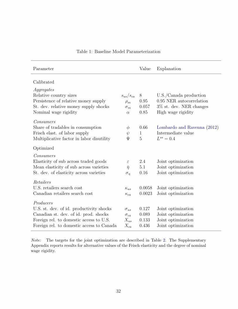
Table 1: Baseline Model Parameterization

Parameter Value Explanation

Calibrated

Aggregates

Relative country sizes sus/sca 8 U.S./Canada productionPersistence of relative money supply ⇢m 0.95 0.95 NER autocorrelationSt. dev. relative money supply shocks �m 0.057 3% st. dev. NER changesNominal wage rigidity ↵ 0.85 High wage rigidity

Consumers

Share of tradables in consumption � 0.66 Lombardo and Ravenna (2012)Frisch elast. of labor supply 1 Intermediate valueMultiplicative factor in labor disutility 5 Lss = 0.4

Optimized

Consumers

Elasticity of sub across traded goods " 2.4 Joint optimizationMean elasticity of sub across varieties ⌘ 5.1 Joint optimizationSt. dev. of elasticity across varieties �⌘ 0.16 Joint optimization

Retailers

U.S. retailers search cost us 0.0058 Joint optimizationCanadian retailers search cost ca 0.0023 Joint optimization

Producers

U.S. st. dev. of id. productivity shocks �us 0.127 Joint optimizationCanadian st. dev. of id. prod. shocks �ca 0.089 Joint optimizationForeign rel. to domestic access to U.S. Xus 0.133 Joint optimizationForeign rel. to domestic access to Canada Xca 0.436 Joint optimization

Note: The targets for the joint optimization are described in Table 2. The SupplementaryAppendix reports results for alternative values of the Frisch elasticity and the degree of nominalwage rigidity.

32

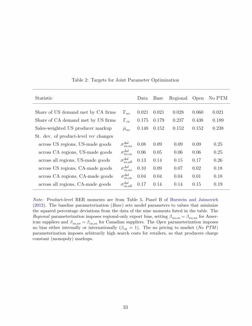
Table 2: Targets for Joint Parameter Optimization

Statistic Data Base Regional Open No PTM

Share of US demand met by CA firms �us 0.021 0.021 0.028 0.060 0.021

Share of CA demand met by US firms �ca 0.175 0.179 0.237 0.438 0.189

Sales-weighted US producer markup µus 0.148 0.152 0.152 0.152 0.238

St. dev. of product-level rer changes

across US regions, US-made goods ��dus,us 0.08 0.09 0.09 0.09 0.25

across CA regions, US-made goods ��dus,ca 0.06 0.05 0.06 0.06 0.25

across all regions, US-made goods ��dus,all 0.13 0.14 0.15 0.17 0.26

across US regions, CA-made goods ��dca,us 0.10 0.09 0.07 0.02 0.18

across CA regions, CA-made goods ��dca,ca 0.04 0.04 0.04 0.01 0.18

across all regions, CA-made goods ��dca,all 0.17 0.14 0.14 0.15 0.19

Note: Product-level RER moments are from Table 5, Panel B of Burstein and Jaimovich(2012). The baseline parameterization (Base) sets model parameters to values that minimizethe squared percentage deviations from the data of the nine moments listed in the table. TheRegional parameterization imposes regional-only export bias, setting �us,ca = �us,us for Amer-ican suppliers and �ca,us = �ca,ca for Canadian suppliers. The Open parameterization imposesno bias either internally or internationally (�rk = 1). The no pricing to market (No PTM )parameterization imposes arbitrarily high search costs for retailers, so that producers chargeconstant (monopoly) markups.

33

Table 3: Estimated Regional and National Bias Parameters

United States Canada

Median Min Max Median Min Max

Cross-region bias �rx 0.32 0.24 0.39 0.14 0.12 0.16Cross-country bias �rx⇤ 0.25 0.25 0.26 0.09 0.08 0.09

Note: Within-region bias is normalized to 1. Cross-region bias is the relative bias against the“away” region of one’s own country. Cross-country bias is the bias against either one of thetwo foreign regions, relative to one’s own region. The median, minimum and maximum valuesare computed over all similarly-sized two-region splits of each country. Nus = 464 possibleequal-sized U.S. splits, and Nca = 108 possible equal-sized Canadian splits.

34

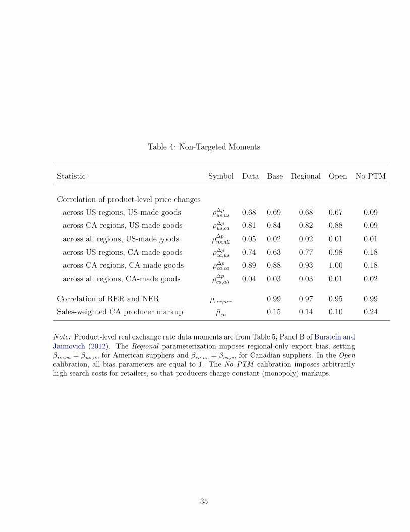
Table 4: Non-Targeted Moments

Statistic Symbol Data Base Regional Open No PTM

Correlation of product-level price changes

across US regions, US-made goods ⇢�pus,us 0.68 0.69 0.68 0.67 0.09

across CA regions, US-made goods ⇢�pus,ca 0.81 0.84 0.82 0.88 0.09

across all regions, US-made goods ⇢�pus,all 0.05 0.02 0.02 0.01 0.01

across US regions, CA-made goods ⇢�pca,us 0.74 0.63 0.77 0.98 0.18

across CA regions, CA-made goods ⇢�pca,ca 0.89 0.88 0.93 1.00 0.18

across all regions, CA-made goods ⇢�pca,all 0.04 0.03 0.03 0.01 0.02

Correlation of RER and NER ⇢rer,ner 0.99 0.97 0.95 0.99

Sales-weighted CA producer markup µca 0.15 0.14 0.10 0.24

Note: Product-level real exchange rate data moments are from Table 5, Panel B of Burstein andJaimovich (2012). The Regional parameterization imposes regional-only export bias, setting�us,ca = �us,us for American suppliers and �ca,us = �ca,ca for Canadian suppliers. In the Opencalibration, all bias parameters are equal to 1. The No PTM calibration imposes arbitrarilyhigh search costs for retailers, so that producers charge constant (monopoly) markups.

35

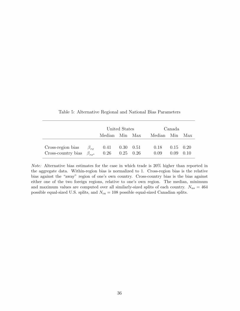
Table 5: Alternative Regional and National Bias Parameters

United States Canada

Median Min Max Median Min Max

Cross-region bias �rx 0.41 0.30 0.51 0.18 0.15 0.20Cross-country bias �rx⇤ 0.26 0.25 0.26 0.09 0.09 0.10

Note: Alternative bias estimates for the case in which trade is 20% higher than reported inthe aggregate data. Within-region bias is normalized to 1. Cross-region bias is the relativebias against the “away” region of one’s own country. Cross-country bias is the bias againsteither one of the two foreign regions, relative to one’s own region. The median, minimumand maximum values are computed over all similarly-sized splits of each country. Nus = 464possible equal-sized U.S. splits, and Nca = 108 possible equal-sized Canadian splits.

36

Supplementary Appendix for

Price Dispersion and the Border E↵ect

Ryan ChahrourBoston College

Luminita StevensUniversity of Maryland

September 18, 2019

A Model Details

Countries are k 2 {US,CA}, sectors/goods are indexed by i 2 [0, 1] and retailers are

indexed by ⌫ 2 [0, 1].

Retailers

The problem of the retailers in each region is described in the main text. Each retailer’s

profit function is the sum of profits obtained from selling its own variety of each good,

(⌫, i). All retailers in country k face the same constant elasticity of demand for each good,

⌘ik, distributed according to ⌘ik ⇠ f⌘. Retailers therefore charge a constant markup

µik = ⌘ik⌘ik�1 over marginal cost. Since di↵erentiation of each good i into the retailer-

specific variety is costless, the retailer’s marginal cost is the producer price at which it

stops the search and purchases all its demand, bpi⌫k. Maximized profits as a function of

the sampled price, bp, are given by

⇡r⇤(bp) = (µik � 1)(µik)�⌘ik(bp)1�⌘ik(Pik)

⌘ikCik.

The retailer’s search decision depends on distribution of prices posted in sector i in

country k, fik. After sampling a price from this distribution, the retailer decides wether

to quit searching (ns) and purchase all demand at the sampled price, or search again (s).

A1

For a given draw bp from the distribution fik, the retailer’s value function is:

V (bp; fik) = max{V ns(bp), V s(fik)}

where

V ns(bp) = ⇡r⇤(bp)

is the profit the retailer earns if they do not continue to search and

V s(fik) = E [V (p; fik)]� k

is the value of repeating the search. Optimal search policy consists of country and sector

specific reservation price rik above which retail firms chose s, and below which they

choose ns.

Producers

Producers in sector i post potentially di↵erent prices in each market. Because we have

assumed that regions within the same country are symmetric, they post the same price in

markets within the same country. Retailers that settle on a given producer have elastic

demand. Hence optimal prices that are below the reservation price will be a constant

markup over producer marginal cost. Since the retailers pass on the demand from the

consumers, producers set the same markup µik over marginal cost. Producers whose

marginal cost is high enough such that they earn no profits at the reservation price

choose to shut down.

A firm producing in country k0 and selling in country k faces the problem

maxpj

(bpj �mcj)xik(bpj)

where

xik(bpj) =

8><

>:

�ik(µikbpj)�⌘ik(pik)⌘ikCik if bpj rik

0 if bpj > rik

A2

and mcj =wk0Aj

, Aj ⇠ fAk, and �ik is the mass of active retailers-per-producer in sector i

in country k at the time. We have assumed that the mass of retailers is equal to the mass

of potential producers, so that �ik � 1, with strict inequality only when some producers

find it optimal to shutdown for the period given retailer’s reservation prices.

Denote the optimal price of the producing in country k0 and selling in k with bp⇤ijk0,k. The

corresponding implied labor demand of the firm is lijk0,k = xik(bp⇤ijk0,k)/Aj. The total labor

demanded by country-k0 traded-good producers is

LTk =

Z 1

0

Z 1

0

lijk0,k1[p⇤ijk0,k �mcj > 0]djdi

| {z }labor supplied to exports

+

Z 1

0

Z 1

0

lijk0,k01[p⇤ijk0,k0 �mcj > 0]djdi

| {z }labor supplied to domestic sales

.

(A.1)

where 1(·) is an indicator function indicating when producer choose to become active.

General Equilibrium and Market Clearing

Individual firm level prices and quantities must be consistent with general equilibrium in

the economy. In addition to the expression for traded-good labor (A.1) above, it must

be that

Cik =

✓Z 1

0

(Ci⌫k)⌘ik�1⌘ik d⌫

◆ ⌘ik⌘ik

(A.2)

CTk =

✓Z 1

0

(Cik)"�1" di

◆ "�1"

(A.3)

pik =

✓Z 1

0

p1�⌘iki⌫k d⌫

◆ 11�⌘ik

(A.4)

P Tk =

✓Z 1

0

p1�"ik di

◆ 11�"

(A.5)

PNk = Wk (A.6)

CTk = �Mk/P

Tk (A.7)

CNk = (1� �)Mk/P

Nk (A.8)

LNk = CN

k /A (A.9)

Lk = LTk + LN

k (A.10)

A3

Given the values for {Mk} for each country and distributions {fAk} and f⌘, equilibrium

in the economy is summarized by a set of reservation prices {rik} selected by retailers,

a distribution of wholesale prices posted {fik} selected by producers, the sets of general

equilibrium objects summarized above, {⌦k}, where

⌦k ⌘�{Cik, pik} , CT

k , CNk , LT

k , LNk , Lk, P

Tk , P

Nk ,Wk

,

and an exchange rate e that ensures balanced trade.

Regional Bias Measures

The measure of firms from k with an opportunity to sell in region k0 is given by the

matching function

mkk0 =�kk0SkSk0

Sk + Sk0.

Hence, imposing symmetric sized regions within each country, the total sales opportuni-

ties for firms in region a of the US is given by

maa +mab =(1 + �ab)S

2a

2Sa= Sa

1 + �ab

2.

The probability that a given region-a firm has a domestic selling opportunity is then just

maa +mab

Sa=

1 + �ab

2.

Similarly, the probably that a given region-a firm has foreign selling opportunity is

mac +mad

Sa=

2�acSc

Sa + Sc.

Hence the relative probabilities of accessing the foreign market relative to the domestic

market — the parameter that is pinned down by the pricing moments we target — is

Rus =2�ac

1 + �ab

⇥ 2Sc

Sa + Sc.

A4

In turn, this pins down the measure of pure bias,

Xus =2�ac

1 + �ab

.

National bias is a composite of both regional bias and additional bias that comes from

crossing the border. To separately identify the regional bias, we derive a relationship

between this parameter and the domestic import share. Given within-country symmetry,

sales per firm have the same distribution regardless of the domestic region of origin.

Hence, we need only compute the ratio of e.g. the number of region b firms with selling

opportunities in region a compared to the total number of firms selling in region a; this

will be equal to the import share. This is given by

�a ⌘mba

mba +maa=

�ab

1 + �ab

.

Hence the internal bias parameters are uniquely identified by trade-quantities alone.

Together with the expression for Xus, this fully identifies our bias parameters. Identical

calculations delivers analogous expressions for the Canada.

B Extension with Menu Costs

As a robustness check, we consider a steady-state version of the economy in which all

shocks remain i.i.d., but producing firms face a menu cost ⌧ k of changing a price posted

in country k from the previous period. Firms entering a given period with a price that is

close enough to their optimal price choose not change their price in the current period.

Let

⇧(bpj) ⌘ (bpj �mcj)xci(bpj)

be the contemporaneous profit of a firm producing firm in sector i charging price bpj and

let bp⇤c be the price that maximizes B. Then, the value function of a producer entering

the period with inherited price pj,t�1 is

V pc(pj,t�1) = max {⇧(bp⇤c)� ⌧ c + E[V pc(bp⇤c)],⇧(pj,t�1) + E[V pc(bpj,t�1)], } . (B.1)

A5

As before, we assume that firms who would earn negative profits if they posted a price

and produced choose to shutdown, and inherit their past price for the subsequent period.

C Numerical Procedure

In order to solve the model, we discretize the state-space and the set of prices that

producing firms may post. There are three states that need to be discretized. We

approximate the distribution of log marginal cost using 200 equally spaced grid between

-5 and +5 standard deviations. The distribution of sectoral elasticities is approximated

by using 16 gaussian hermite grid points to approximate the bivariate normal distribution

for elasticities in each sector for both countries. Finally, the set of aggregate monetary

shocks is approximated for each country using the Rouwenhorst (Kopecky and Suen

(2010)) approach to create a 3 point discrete markov process that approximates and

AR(1) process with persistence 0.95. Finally, optimal prices are computed on a grid of

600 equally-spaced grid of potential (log) prices.

We use an iterative approach to solve for the equilibrium of the economy. We conjecture

an initial set of general equilibrium prices and quantities (summarized above), compute

optimal pricing decision by firms, find implied quantities and labor demand, and use the

results to update the general equilibrium quantities. Since this is a steady-state model,

we require balanced trade. Our iterative procedure adjusts the nominal exchange rate to

ensure trade is balanced.

Given the number of discrete choices in the model, the iterative algorithm sometime

oscillates between very similar solutions without fully converging. We have found that

this can generally be avoided by assuming that firms’ choice to shutdown or operate

adjust continuously in the neighborhood of zero profits, rather than discretely shutting

on or o↵. We implement this using the an exponential function, so that the probability

of shutting down is

pshut =exp(V shut/�)

exp(V shut/�) + exp(V open/�),

with � = 0.0002. This ensures that, in equilibrium, pshut is numerically zero or one for

all but a small number of firms very close to indi↵erent between operating and shutting

A6

down.

For each state in the aggregate state-space, our numerical algorithm can be summarized

as an iteration l = 0, 1, ... on the following steps:

1. Conjecture a set of general equilibrium objects in both countries, including k- and

i-specific prices and quantities, reservation prices, general equilibrium quantities

{⌦k}l, and the bilateral exchange rate.

2. Given the entries in {⌦k}l and the reservation prices, compute the optimal prices

(or shutdown decision) for for producers from each country and for each value of

the marginal cost grid. This implies a distribution of prices posted in each country,

fik.

3. Given {fik}, compute the optimal search decision of retailers and update reservation

prices, {rik}.

4. Given the distribution of {fki} and {rik}, compute the implied quantities and price

indexes and update (or partially update) the entries of {⌦k}l + 1.

5. Check if |{⌦k}l+1 � {⌦k}l| ⇡ 0. If not, return to step 1.

D Additional Results

Alternative model versions: Table D.1 presents results for the steady state and

for the best-fitting menu cost model. The first column presents values for the baseline

estimation; the second column presents values for the stochastic steady state with id-

iosyncratic shocks but no aggregate shocks; and the third column presents values for the

best-fitting menu cost model.

When we compare the model to the data, we compute the model statistics based on the

equilibrium with both idiosyncratic and aggregate shocks, aggregated over many periods.

Our empirical moments are based on data during “normal times”, with no recession or

large expansion during the sample period. Nevertheless, the statistics at the steady state

with no aggregate shocks are close to the baseline statistics.

A7

For the menu cost model, the national bias parameters, Xus and Xca, are kept fixed at

values we estimated in our baseline model. We then re-estimate the model, targeting the

same set of moments as the baseline model, along with a price change frequency of 1/3

in both the U.S. and Canada. The model generates dispersion statistics that are similar

to those generated by the flexible price model. Since these moments are obtained with

the same values for the international access parameters, the estimation implies exactly

the same coe�cients for regional versus international segmentation. We conclude that

adding nominal rigidities does not alter our inference regarding the severity of regional

versus national trade frictions.Introducing the nominal price rigidity does a↵ect some of

the other estimated parameters. In particular, it yields larger idiosyncratic productivity

shocks and smaller markup shocks, compared with the flexible price model. Since nominal

rigidities generate endogenous variation in realized markups, the model requires smaller

elasticity shocks to generate the same level of price dispersion. The estimation also yields

higher search and menu costs for Canada compared with the U.S.

Robustness: Table D.2 presents sensitivity results to alternative parameterizations.

For the Frisch elasticity, the article reports results for an intermediate value of the Frisch

elasticity equal 1. Here, we report results for 0.4 (which is closer to the estimates based on

micro data) and 1.5 (which is towards the high end of the values used in macro models),

per Chetty et al. (2011) and Keane and Rogerson (2012). Results are modestly a↵ected.

In particular, a higher Frisch elasticity raises markups, and hence price dispersion, and

generates a lower correlation of price changes both within and across countries, but our

conclusions do not change qualitatively. Note that although the micro literature suggests

small elasticities, structural work has shown that small micro elasticities can coexist with

large macro elasticities, which means that higher values are warranted for representative

agent macro models like ours.

For the degree of wage rigidity, the article reports results for a high wage rigidity param-

eterization (↵w = 0.85). To a simple approximation, this level of rigidity is equivalent

to assuming a Calvo model in which wages are reoptimized roughly every six quarters.

This is somewhat higher than the micro-based estimates of Barattieri et al. (2014), who

report an estimated duration of 4 to 5 quarters, based on survey data corrected for mea-

A8

surement error. The values estimated in DSGE models typically range from 2.8 quarters

(Christiano, Eichenbaum and Evans, 2005) to nearly 4 quarters (Smets and Wouters,

2007). Our relatively higher degree of wage rigidity reflects the fact that what matters

for aggregate dynamics is the extent to which wages incorporate new information, which

is a↵ected by both the frequency of adjustment and the degree of noise and inertia con-

ditional on adjustment. Below, we report results for a lower degree of wage rigidity equal

to 0.65 (close to the CEE estimates). Overall, our results are very robust to changes in

the degree of wage rigidity. With a lower degree of wage rigidity, both the volatility of

the NER and the correlation of price changes across the border (which is an untargeted

moment) increase. The remaining statistics do not change in significant ways.

Lastly, our baseline results estimate a small amount of volatility in the elasticity of substi-

tution among varieties. As discussed in the main text, this volatility in desired markups

enables us to generate large price dispersion without also generating large aggregate

fluctuations. Below we report results for the case of an even smaller variation in this

elasticity (0.04 instead of 0.16). We find that this generates less trade, less cross-country

price dispersion, and a much lower correlation of price changes.

The Role of Asymmetries: We incorporate multiple dimensions of asymmetry in our

parameterization: market size, trade bias, productivity dispersion among producers, and

search costs for retailers. While the last two dimensions are crucial for matching the price

dispersion data, the first two are particularly important for matching trade volumes, as

shown in Table D.3, which reports results for two alternative specifications: one in which

the two countries are both equal to the average between the U.S. and Canada, and one

in which the two countries have the same retailer search costs and the same producer

productivity dispersion, and these parameters are set to the average between the U.S.

and Canada.

Regional Heterogeneity Our results show that how the subregions are aggregated

matters for estimates of internal segmentation, especially for the U.S. But they also

suggest that the bias against foreign producers is roughly symmetric: the ranges of

values for �us,ca and �ca,us are quite narrow.

A9

For the U.S., the regional bias coe�cients range from 0.24 to 0.39. This means that

economic integration is uneven across subregions. It is indeed the case that proximity

plays a role in segmenting U.S. regions, as shown in Figure D.1, but its explanatory power

is quite limited. For Canada, regional segmentation is more severe, but it is also more

narrow. Furthermore, there is virtually no correlation with distance, and there also does

not appear to be a stronger regional bias between Quebec and the rest of Canada. We

leave for future work a theory of endogenous regional bias, which would likely require

modeling the network structure of each country.

A10

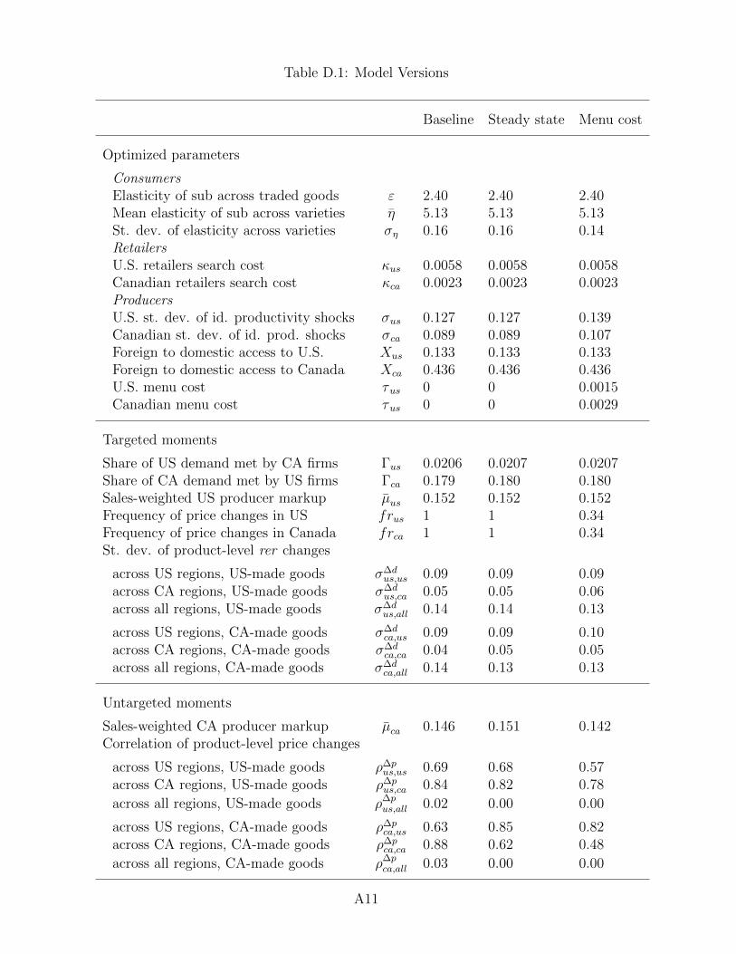
Table D.1: Model Versions

Baseline Steady state Menu cost

Optimized parameters

ConsumersElasticity of sub across traded goods " 2.40 2.40 2.40Mean elasticity of sub across varieties ⌘ 5.13 5.13 5.13St. dev. of elasticity across varieties �⌘ 0.16 0.16 0.14RetailersU.S. retailers search cost us 0.0058 0.0058 0.0058Canadian retailers search cost ca 0.0023 0.0023 0.0023ProducersU.S. st. dev. of id. productivity shocks �us 0.127 0.127 0.139Canadian st. dev. of id. prod. shocks �ca 0.089 0.089 0.107Foreign to domestic access to U.S. Xus 0.133 0.133 0.133Foreign to domestic access to Canada Xca 0.436 0.436 0.436U.S. menu cost ⌧us 0 0 0.0015Canadian menu cost ⌧us 0 0 0.0029

Targeted moments

Share of US demand met by CA firms �us 0.0206 0.0207 0.0207Share of CA demand met by US firms �ca 0.179 0.180 0.180Sales-weighted US producer markup µus 0.152 0.152 0.152Frequency of price changes in US frus 1 1 0.34Frequency of price changes in Canada frca 1 1 0.34St. dev. of product-level rer changes

across US regions, US-made goods ��dus,us 0.09 0.09 0.09

across CA regions, US-made goods ��dus,ca 0.05 0.05 0.06

across all regions, US-made goods ��dus,all 0.14 0.14 0.13

across US regions, CA-made goods ��dca,us 0.09 0.09 0.10

across CA regions, CA-made goods ��dca,ca 0.04 0.05 0.05

across all regions, CA-made goods ��dca,all 0.14 0.13 0.13

Untargeted moments

Sales-weighted CA producer markup µca 0.146 0.151 0.142Correlation of product-level price changes

across US regions, US-made goods ⇢�pus,us 0.69 0.68 0.57

across CA regions, US-made goods ⇢�pus,ca 0.84 0.82 0.78

across all regions, US-made goods ⇢�pus,all 0.02 0.00 0.00

across US regions, CA-made goods ⇢�pca,us 0.63 0.85 0.82

across CA regions, CA-made goods ⇢�pca,ca 0.88 0.62 0.48

across all regions, CA-made goods ⇢�pca,all 0.03 0.00 0.00

A11

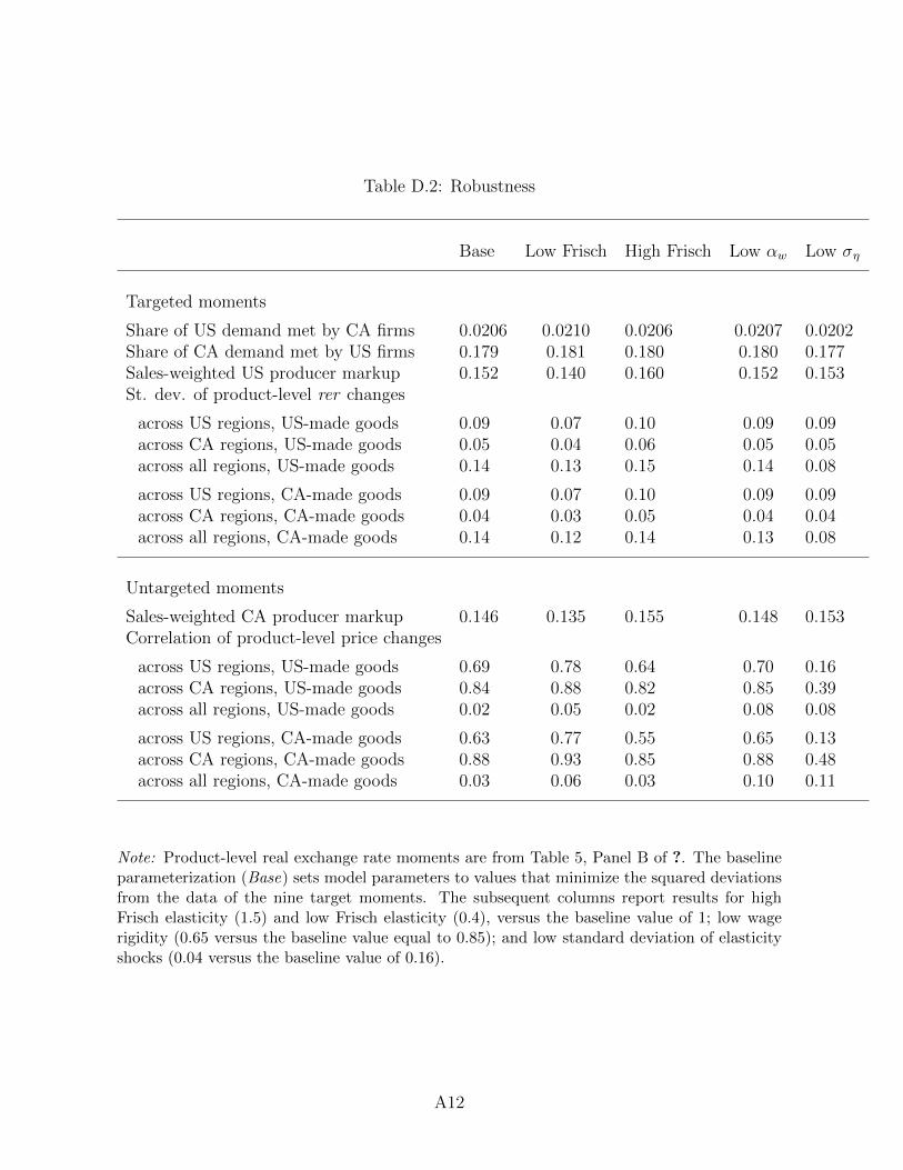
Table D.2: Robustness

Base Low Frisch High Frisch Low ↵w Low �⌘

Targeted moments

Share of US demand met by CA firms 0.0206 0.0210 0.0206 0.0207 0.0202Share of CA demand met by US firms 0.179 0.181 0.180 0.180 0.177Sales-weighted US producer markup 0.152 0.140 0.160 0.152 0.153St. dev. of product-level rer changes

across US regions, US-made goods 0.09 0.07 0.10 0.09 0.09across CA regions, US-made goods 0.05 0.04 0.06 0.05 0.05across all regions, US-made goods 0.14 0.13 0.15 0.14 0.08

across US regions, CA-made goods 0.09 0.07 0.10 0.09 0.09across CA regions, CA-made goods 0.04 0.03 0.05 0.04 0.04across all regions, CA-made goods 0.14 0.12 0.14 0.13 0.08

Untargeted moments

Sales-weighted CA producer markup 0.146 0.135 0.155 0.148 0.153Correlation of product-level price changes

across US regions, US-made goods 0.69 0.78 0.64 0.70 0.16across CA regions, US-made goods 0.84 0.88 0.82 0.85 0.39across all regions, US-made goods 0.02 0.05 0.02 0.08 0.08

across US regions, CA-made goods 0.63 0.77 0.55 0.65 0.13across CA regions, CA-made goods 0.88 0.93 0.85 0.88 0.48across all regions, CA-made goods 0.03 0.06 0.03 0.10 0.11

Note: Product-level real exchange rate moments are from Table 5, Panel B of ?. The baselineparameterization (Base) sets model parameters to values that minimize the squared deviationsfrom the data of the nine target moments. The subsequent columns report results for highFrisch elasticity (1.5) and low Frisch elasticity (0.4), versus the baseline value of 1; low wagerigidity (0.65 versus the baseline value equal to 0.85); and low standard deviation of elasticityshocks (0.04 versus the baseline value of 0.16).

A12

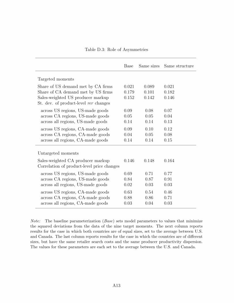
Table D.3: Role of Asymmetries

Base Same sizes Same structure

Targeted moments

Share of US demand met by CA firms 0.021 0.089 0.021Share of CA demand met by US firms 0.179 0.101 0.182Sales-weighted US producer markup 0.152 0.142 0.146St. dev. of product-level rer changes

across US regions, US-made goods 0.09 0.08 0.07across CA regions, US-made goods 0.05 0.05 0.04across all regions, US-made goods 0.14 0.14 0.13

across US regions, CA-made goods 0.09 0.10 0.12across CA regions, CA-made goods 0.04 0.05 0.08across all regions, CA-made goods 0.14 0.14 0.15

Untargeted moments

Sales-weighted CA producer markup 0.146 0.148 0.164Correlation of product-level price changes

across US regions, US-made goods 0.69 0.71 0.77across CA regions, US-made goods 0.84 0.87 0.91across all regions, US-made goods 0.02 0.03 0.03

across US regions, CA-made goods 0.63 0.54 0.46across CA regions, CA-made goods 0.88 0.86 0.71across all regions, CA-made goods 0.03 0.04 0.03

Note: The baseline parameterization (Base) sets model parameters to values that minimizethe squared deviations from the data of the nine target moments. The next column reportsresults for the case in which both countries are of equal sizes, set to the average between U.S.and Canada. The last column reports results for the case in which the countries are of di↵erentsizes, but have the same retailer search costs and the same producer productivity dispersion.The values for these parameters are each set to the average between the U.S. and Canada.

A13

0 500 1000 1500 2000Distance in KM

0.22

0.25

0.28

0.31

0.34

0.37

0.4

Cro

ss-re

gion

bia

s (

r2)

US

R2 = 0.140

0 500 1000 1500 2000 2500

0.12

0.13

0.14

0.15

0.16

CA

R2 = 0.018

Figure D.1: Scatter plot of regional bias against distance

A14

References

Barattieri, A., S. Basu, and P. Gottschalk (2014). Some evidence on the importance of

sticky wages. American Economic Journal: Macroeconomics 6 (1), 70–101.

Benabou, R. (1988). Search, price setting and inflation. The Review of Economic Stud-

ies 55 (3), 353–376.

Benabou, R. and R. Gertner (1993). Search with learning from prices: Does increased in-

flationary uncertainty lead to higher markups? The Review of Economic Studies 60 (1),

69–93.

Burdett, K. and G. Menzio (2017). The (Q, S, s) pricing rule. The Review of Economic

Studies 85 (2), 892–928.

Chetty, R., A. Guren, D. Manoli, and A. Weber (2011). Are micro and macro labor

supply elasticities consistent? a review of evidence on the intensive and extensive

margins. The American Economic Review 101 (3), 471–475.

Christiano, L. J., M. Eichenbaum, and C. L. Evans (2005). Nominal rigidities and the

dynamic e↵ects of a shock to monetary policy. Journal of Political Economy 113 (1),

1–45.

Keane, M. and R. Rogerson (2012). Micro and macro labor supply elasticities: A re-

assessment of conventional wisdom. Journal of Economic Literature 50 (2), 464–76.

Kopecky, K. A. and R. M. H. Suen (2010). Finite state Markov-chain approximations to

highly persistent processes. Review of Economic Dynamics 13 (3), 701–714.

Smets, F. and R. Wouters (2007). Shocks and frictions in US business cycles: A Bayesian

DSGE approach. American Economic Review 97 (3), 586–606.

15