1

Price and Wage Inflation in Chile

Carlos Jose García T. & Jorge Enrique Restrepo✝

Central Bank of Chile

Abstract

Price and wage equations based on a model of imperfect competition were estimated using data from 1986:1 to 2000:4. From the estimations we can conclude: (i) as expected, productivity reduces unit labor costs and inflation and increases real wages; (ii) it is confirmed what was found in other studies in the sense that output gap and unemployment have a small impact on inflation due to widespread indexation; (iii) inflation imposes important costs to firms and workers; (iv) the exchange rate pass-through depends positively on economic activity and the inflation level, explaining why pass-through has been so low in recent years. Since inflation has been stabilized around 3% Pass-through should be permanently lower than in the nineties. The estimation includes the first difference of the dependent variable following the literature on the estimation of linear quadratic adjustment cost (LQAC) models when the target and some of the driving variables follow I(2) processes. Given that it is a mark-up model, the price index fitted is narrower than the CPI to reflect the fact that these prices are formed where there is monopolistic competition. In order to model wages, we assume that a fraction of wages is negotiated, while the other fraction is adjusted according to past inflation. The nominal wages negotiated are determined following the theory of efficiency wage and bargaining model. The equations are used to generate out-of-sample inflation forecast closer to actual inflation than before.

JEL Classification: F3, F4 Key Words: Exchange rate pass-through, Phillips curve, mark-ups

✝ Senior Economists, Central Bank of Chile The views expressed in this paper are those of the authors and should not be attributed to the Central Bank of Chile. We would like to thank Pablo García, Esteban Jadresic and seminar participants at the Bank of International Settlements and the Central Bank of Chile, for their comments and suggestions.

2

Contents

I. Introduction

II. Inflation Stylized Facts and Theoretical Considerations

a. The Phillips Curve

b. Exchange Rate Pass-Through

i. Theory and international evidence

ii. Rolling correlation

iii. Rolling regression and pass-through in a small-structural model

III. A Price Setting Model

a. Optimal price in the long run

b. Short run

IV. Results

a. Unit Roots and Cointegration

b. Price equation

c. Wage equation

d. Pass-Through

V. Conclusions

3

I. Overview

This article estimates equations for price and wage inflation using quarterly Chilean data

from 1986:1 to 2000:4. Several issues crucial for understanding and anticipating the

behavior of inflation —which are at stake in the Phillips curve— motivate such

estimation. For instance: i) elasticity of inflation to the output gap, ii) the permanent and

cyclical movements of mark-ups, iii) effects of labor productivity growth on inflation, iv)

credibility, indexation and rationality, and v) the size of the exchange rate pass-through.

Even though we touch all these subjects in this paper, we take a closer look at the effect

of exchange-rate changes on domestic inflation because apparently this factor has

substantially changed in recent years. Despite the fact that Chile is a small open

economy, the exchange rate pass-through has been low recently. In fact, there has been

significant peso depreciation since 1997 without having a strong impact on inflation.

Why is it? Is a low pass-through a new permanent characteristic of the Chilean economy?

Will the depreciation impact on inflation take place as soon as demand takes off again?

The answer to these questions is crucial defining monetary policy.

In order to tackle at least part of this research agenda, we present below a model of the

Phillips curve based on some microfoundations and time-series econometrics. Thus, we

address these issues by estimating a structural equation for price inflation that considers

explicitly a model of staggered nominal price setting by imperfect competitive firms. In

doing this, we use the quadratic price adjustment cost model of Rotemberg (1982), where

the representative firm chooses a sequence of prices for solving its intertemporal

problem. As a result, inflation can be represented as an error correction equation (Euler

equation), relating this variable to expected inflation as well as to the gap between the

“equilibrium” and actual price level.

In addition, an I(2) analysis of inflation and the mark-up is undertaken. We find that the

price level is best described as I(2) process. To deal with I(2) processes, we incorporate

inflation as an additional component of the “equilibrium” price in the Euler equation

(Engsted and Haldrup 1999). Having this variable in the cointegration equation reflects

the existence of a long-run relationship between mark-ups and inflation. In the

4

estimations this relationship is negative, which may be interpreted as the cost to firms of

overcoming missing information when adjusting prices in an inflationary environment

(Barnerjee, Cockerell and Russell 2001). Different versions of the price equation are

estimated (Gruen, Pagan and Thompson 1999) by using a limited-information approach

due to McCallum (1976).

Since, there is a clear connection between prices and wages, we also estimated a model to

explain wage dynamics. The model assumes that a fraction of wages is negotiated every

period, while the other fraction is adjusted according to past inflation (Jadresic 1996).

The negotiated nominal wages are determined following the theory of efficiency wage

and the bargaining model. Thus, expected real wages depend on labor productivity,

unemployment, and past real wages (Blanchard and Katz 1997). In order to incorporate

the fact that nominal wages are also I(2), we included the inflation rate as a cost for

workers when wages are negotiated. Since indexation is never perfect, the higher the

inflation level, the lower real average wage each period.

The results show, as expected, that labor productivity reduces unit labor costs and

inflation. In addition, a negative relationship between inflation and both mark-ups and

real wages indicates that inflation imposes important costs for firms and workers, fully

justifying the stabilization program put in place by the Central Bank since 1990.

Moreover, the results confirm what was found in other studies in the sense that output

gap and unemployment have a small impact on inflation due to widespread indexation.

Therefore, gradual monetary policy is perfectly adequate in this case.

Finally, since pass-through is related to economic activity and the level of inflation, it

should be smaller than in the nineties given that the level of inflation has been stabilized

around 3%. Taking the estimated price and wage equations simultaneously, the

exchange-rate pass-through is analyzed by simulating an exchange rate shock, with and

without output gap. Had not existed a negative output gap after 1997 exchange rate pass-

through would have been higher.

5

This article is organized as follows. The second section shows several stylized facts and

introduces some imperfect-competition theoretical framework for the Phillips curve and

the exchange rate pass-through. The third one presents the mark-up model for prices. The

next section has a wage model based on indexation, efficiency wage, and bargaining

models. Then, the fourth section presents the estimations for the price and wage

equations. Finally there are some conclusions and policy recommendations.

II. Inflation Stylized Facts and Theoretical Considerations

Figure 1 was built with data covering the sample already mentioned. It shows that during

this period quarterly inflation has had a positive correlation with output gap and foreign

inflation (considering the depreciation rate as well). Where output gap was calculated as

the difference between actual output and its Hodrick-Prescott trend. Meanwhile, inflation

had a negative correlation with average labor-productivity growth. The strong relation

between price and nominal wage inflation indicates the key role indexation plays in the

Chilean economy. In addition it is important to point out that there is a negative

correlation between inflation and the mark-up1. This reveals that, contrary to what we

initially expected, in periods of higher inflation it is much harder for firms to increase the

mark-up.

The negative correlation between real wages and inflation also indicates that workers

suffer important costs from the latter expressed in lower real wages. Furthermore, both

labor productivity and unemployment are important in wage setting as well. As seen in

Figure 1 both variables have a strong correlation with real wages but with different signs.

These graphs seem to indicate there is a Phillips curve with a small slope while other

variables, such as labor productivity and foreign inflation, also play an important role

explaining inflation.

1 Mark-up is obtained as the error term of this equation ttttt paqwaap ε++−+= *)( 210 . Pt is price level, wt is nominal wage, p*

t is foreign price (adjusted by exchange rate, tariff, and taxes).

6

Figure 1 Inflation in Chile: Stylized Facts

a. A Phillips curve

A convenient and widely used setup to describe the behavior of the short-run tradeoff

between the change in inflation and output is the expectations-augmented Phillips curve,

like the one shown in equation 1.

tttttt RmkgapepE εββββπβπβπ ++∆++∆++= +− ******* 654431211 (1)

Where Eπt+1= expected inflation, ∆4ep* = annual imported price inflation, gap = output

gap, ∆mk = mark-up, R = raw materials, supply shocks or relative price changes (Romer

1996, Ball and Mankiw 1995).

Equation 1 is also useful to summarize some of questions already mentioned above in

which we are interested, since the coefficients are associated for instance to: i) 1β : inertia

and 2β : how much forward looking price formation is; ii) 3β : the size of the exchange

.00

.01

.02

.03

.04

.05

.06

.07

-.08 -.04 .00 .04 .08

Output Gap(-1)

Infla

tion

Inflation and Output Gap

-.06

-.04

-.02

.00

.02

.04

.06

.00 .02 .04 .06 .08

Inflation

Mar

kup

Inflation and Markup

.00

.01

.02

.03

.04

.05

.06

.07

-.05 .00 .05 .10 .15

Foreign Inflation

Infla

tion

Inflation and Foreign Inflation

.00

.01

.02

.03

.04

.05

.06

.07

-.02 .00 .02 .04

Productivity Growth

Infla

tion

Inflation and Productivity Growth

.00

.01

.02

.03

.04

.05

.06

.07

.00 .04 .08 .12

Nominal Wage Growth

Infla

tion

Inflation and Nominal Wage Growth

.1

.2

.3

.4

.5

.6

.7

5.4 5.5 5.6 5.7 5.8 5.9 6.0 6.1

Productivity

Rea

l Wag

e

Productivity and Real Wage

.1

.2

.3

.4

.5

.6

.7

.00 .02 .04 .06 .08

Inflation

Rea

l Wag

e

Inflation and Real Wage

.1

.2

.3

.4

.5

.6

.7

.04 .06 .08 .10 .12

Unemployment Rate

Rea

l Wag

e

Unemployment Rate and Real Wage

7

rate pass-through; iii) 4β : elasticity of inflation to the output gap; iv) 5β : the effect of

mark-ups on inflation; v) 6β : effects of raw- material shocks on inflation2.

Similar or variations of equation 1 have been estimated for Chile (García, Herrera, and

Valdés 2000). Nonetheless it is useful to pursue further research on Phillips curves since

there is uncertainty about the β parameters, they do not have a structural interpretation

and finally some of those equations have consistently overpredicted Chilean inflation

during the recent past.

Furthermore, we will follow a different approach: instead of estimating a reduced form

relation between the change in inflation and the unemployment rate we will estimate

separate price and wage equations based on a model of imperfect-competitive firms in

error-correction form. Thus, the error correction in the price equation ensures that in the

steady state the price level is a mark-up on unit labor costs.

Besides the issues cited above, estimating price and wage equations will also allow us to

say something about the relationship between labor productivity and inflation, and the

effects inflation has on mark-ups and wages. The non-competitive setting is also

appropriate to analyze the low exchange-rate passthrough experienced in recent years.

Getting the right size of this coefficient is instrumental in implementing an adequate

monetary policy. In the next section we introduce the non-competitive theoretical

framework by relating the exchange rate pass-through to mark-ups and imperfect

competition.

b. Pass-Through from Depreciation to Inflation

i. Theory

Although the exchange rate directly affects the peso price of imported goods, this

movement does not necessarily get transferred to the end consumer immediately. When

does this transfer occur and to what degree depends on several factors, some of which are

described below.

2 1β and 2β coefficients are usually restricted to add up to 1.

8

As above said, the impact of changes in the exchange rate on domestic inflation is known

as the “pass-through coefficient”. The direct short-term effect of the exchange rate on

inflation is related to the imported part of the basket of goods that make up the CPI. The

larger the share of imported goods within the CPI basket, the greater the exchange rate

effect on prices. In Chile, about 48% of CPI goods are considered importable. The

exchange rate also directly affects the cost structure of companies using imported inputs.

Thus, the greater the proportion of imported inputs making up the costs, the more

depreciation will affect these companies’ prices.

In a regime based on inflation targets, pass-through ultimately depends on monetary

policy and agents’ expectations. Although in the short-term inflation may rise due to

depreciation, in the medium- and long-term inflation should fall back to the target level

or range defined by the Central Bank.

The behavior of demand determines whether or not companies can transfer to end prices

any changes in their costs resulting from fluctuations in the exchange rate. For example,

if the economy is in the midst of a recession, companies will find it difficult to transfer to

their prices higher costs due to depreciation. Furthermore, movements in the exchange

rate can also influence both the level of aggregate demand and wages as well as the

composition of demand. For example, depreciation in the exchange rate that tends to

produce a contraction in aggregate demand could also end up reducing prices by an

amount equivalent to the upward pressures generated by the same depreciation.

Currency devaluation brings with it a change in relative prices. Assuming that income is

constant, when the prices of imported goods rise, consumers’ real income falls. If demand

for these imported goods is inelastic, the purchase of other goods and services will have

to fall and, as a result, so will the prices of the latter, assuming that prices are perfectly

flexible. However, prices are often rigid due to market imperfections. In this case, faced

with currency depreciation, the CPI inflation rise. This is why many pass-through

analyses are based on aspects related to industrial organization (Dornbusch, 1987). This

analysis emphasizes, for example, the degree of import penetration, market structure in

9

terms of greater or lesser concentration, and the differentiation and degree of substitution

between domestic and imported products.

A greater concentration in a productive sector increases the producing company’s control

over price and therefore over profit margins (mark-ups). The same occurs if there is a

small degree of substitution between the domestic and imported product. This degree of

control over the price could vary with the cycle (Small 1997). In these situations,

producers evaluate the costs of modifying their prices and when these are higher than the

benefits, they accept transitory fluctuations in their profit margins, causing prices to react

less to shifts in the exchange rate.

As a result, in the presence of imperfect competition, aggregate demand movements,

combined with fluctuations in the exchange rate, affect importers’ mark-ups. More

volatile aggregate demand would be associated with a reduced pass-through of exchange

rate fluctuations to end prices. In this case, importers will be less willing to raise their

prices for fear of losing market share.

The entrance of new firms could have an impact similar to a demand reduction. For

instance, during the nineties the retailing sector has gone through a restructuring process

in Chile. As a matter of fact, huge superstores and supermarkets distributing a wide

variety of products proliferated. These megastores are usually able to reduce costs

because of their ability to negotiate with suppliers. At the same time they fight for their

market share by introducing sales and different marketing strategies. Some times these

sales imply mark-up reduction particularly when demand is weak.

The volatility of the exchange rate is another factor influencing transfers affecting

domestic inflation. Thus, the more volatile the exchange rate, the less its impact on

domestic prices should be, because importers will be more cautious when it comes to

changing prices, especially when the costs of an adjustment are high. As a result,

expectations about the duration of currency depreciation affect the speed and size of pass-

through of a higher exchange rate to prices.

10

The level of inflation also affects the pass-through coefficient. In general, the magnitude

of the transfer should fall as the annual inflation rate declines. In a low-inflation

economy, the price change of a good is more easily perceived as a modification of

relative prices, which has more impact on demand for the good and its market share.

Thus, the cost of increasing prices could be high for a company, if its market share plays

a decisive role in its margins and total profits (Taylor 2000).

International evidence indicates that the pass-through of the exchange rate to prices is

lower in developed countries than in Latin America and Asia3. In one panel estimate with

71 countries, Goldfjan and Werlang (2000) found a depreciation-to-inflation pass-through

coefficient of 0.73 at the end of 12 months. When the sample was sorted between OECD

members (Organization for Economic Cooperation and Development) and emerging

economies, at the end of 12 months, pass-through coefficients of 0.6 and 0.91

respectively appeared. When this sample was sorted by regions, the 18-month coefficient

for Europe was 0.46, while in America it was 1.24. Finally, as a result of an exercise

based on their estimates, the authors found a bias toward predicting higher inflation than

that actually observed in several well-known cases of large depreciation.

ii. Rolling Correlation

The simplest exercise one can do is to compute the correlation between inflation and

exchange rate depreciation. In this case two rolling correlation statistics were computed

(Figure 2). The first one (black line) has its starting date fixed (1986:1) and the

correlation coefficient is calculated each time after adding a new observation starting in

1990. Therefore, each computation has a larger sample than the last one. Even though

this coefficient is rather stable, it has some movement. It decreases at the beginning of the

nineties, grows again from 1994 to 1996 and is steadily falling since 1998.

3 There has been a great amount of articles written on pass-through over the years. Most of them try to estimate how much exchange rate fluctuations are responsible for the behavior of inflation. Some use CPI inflation others producer price inflation. There is also a wide range of estimation techniques used to obtain a quantitative result. It goes from ordinary least squares (Woo 1984), to panel data (Goldfajn and Werlang 2000), vector auto regression (McCarthy 1999), cointegration analysis and error correction models (Beaumont et al 1994, Kim K. 1998, Kim Y. 1990), and state-space models (Kim Y. 1990).

11

Figure 2 Rolling Correlation Coefficient between Annual Inflation and Depreciation

-0 .8

-0 .6

-0 .4

-0 .2

0 .0

0 .2

0 .4

0 .6

0 .8

1 .0

Ene

-90

Ene

-91

Ene

-92

Ene

-93

Ene

-94

Ene

-95

Ene

-96

Ene

-97

Ene

-98

Ene

-99

Ene

-00

The second statistic in Figure 2 (gray line) has a fully moving sample. Thus, both the

starting and ending dates move each time the correlation coefficient is computed. In this

case the statistics fluctuates much more. This coefficient moves closely to what is

happening to the former up to 1996. After that year it falls dramatically to even become

negative showing an important change in the relationship between these two variables.

It is worth saying that such a simple exercise shows that decision making based

exclusively on the pass-through coefficient used in the small structural model, or based

on the first correlation statistics computed, could lead to policy mistakes. That way one

could easily overestimate forecasted inflation missing the significant change, that took

place from 1997 to 1999, in the relationship between inflation and currency depreciation.

iii. Rolling Regression and Pass-Through in a Small Model

A rolling regression was estimated for annual inflation with exchange rate depreciation

and a trend as right hand side variables using monthly data between 1986 and 20004

(Figure 3). Again the two types of rolling samples were used. The left side in Figure 3

shows the regression coefficient obtained when the initial date of the sample does not

change. On the contrary, the sample used to estimate the right side in Figure 3 has both

initial and last date moving. The left panel of Figure 3 shows that the coefficient fall

4 Annual CPI inflation was found to be trend stationary using monthly data.

12

started earlier in 1996. As one would expect the coefficient is less stable with both dates

moving5.

Figure 3 Rolling Regression

0.05

0.15

0.25

0.35

0.45

0.55

0.65

Ene-9

4Ju

l-94

Ene-9

5Ju

l-95

Ene-9

6Ju

l-96

Ene-9

7Ju

l-97

Ene-9

8Ju

l-98

Ene-9

9Ju

l-99

Ene-0

0Ju

l-00

0.05

0.10

0.15

0.20

0.25

0.30

0.35

0.40

0.45

0.50

Ene-9

4Ju

l-94

Ene-9

5Ju

l-95

Ene-9

6Ju

l-96

Ene-9

7Ju

l-97

Ene-9

8Ju

l-98

Ene-9

9Ju

l-99

Ene-0

0Ju

l-00

Missing variables such as output gap may cause the instability problem. We also

simulated a (five equation) small structural model, similar to the one in García, Herrera

and Valdés (2000). The impact of the exchange rate on inflation is controlled by output

gap. The pass-through obtained with this simulation amounts to 50% over 5 to 6 years

(Figure 4). Meaning that the period over which the full impact of a depreciation is felt is

rather long. However, Figure 4 shows that over the first three years most of the effect has

already taken place. It is important to point out that this model includes a monetary rule

consistent with the behavior of a Central Bank in an inflation-targeting regime.

Therefore, it explains why pass-through is never complete in Figure 46.

5 As a matter of fact, it matches some stylized facts of the economy during the last decade. It is well known there was a consumption boom between 1995 and 1997 which coincides with a rebound of this coefficient. 6 Pass-through never reaches 100% because traded goods represent a share of all inputs and consumer goods.

13

Figure 4 Pass-Through in a Small Model

Exchange rate Pass-throughCPI

0.00

0.05

0.10

0.15

0.20

0.25

1 3 5 7 9 11 13 15 17 19 21 23 25

0%

10%

20%

30%

40%

50%

60%

1 3 5 7 9 11 13 15 17 19 21 23 25

III. A Price Setting Model

a. Optimal Price in the Long Run

In this section we derive a Phillips curve from the quadratic price adjustment cost

model developed by Rotemberg (1982). Thus, firms weigh the cost of changing prices

against the cost of being away from the price that the firm would choose in case there

were no adjustment cost (Roberts 1995). The latter price is called the “optimal price”

which is found following Beaumont et al (1994) and Layard et al (1991). The firms are

identical and get an output (y) by using labor (l) and an imported input (z):

iii zalaay )1( 221 −++= (2)

Each firm’s demand is yd-f, where f is the log of the number of identical firms. The

demand curve faced by each firm would be:

( ) fyppy didi −+−−= ~η (3)

where pi is the firm's price, p is the price level and η is the elasticity of demand.

Therefore, the price that maximizes benefits in the long run is given by:

*221 )1(

1log~

ttdi pawaamMCmMCn

np −+++=+=+

−−= (4

where the price (pdi) is fixed by charging a margin (m) over the marginal cost (MC)7. A

pricing model based on a mark-up over costs is inappropriate when applied to markets

close to perfect competition like the ones for agricultural products (Woo 1984). Since the

7 Note also that wt can be separated in private (wprt) and public wages (wput).

14

price index to be explained should be the one reflecting monopolistic markets, core or

underlying inflation, IPCX28 is used here.

We examine the margin now. It is assumed that in the long term firms desire a constant

mark-up, m. However, in the short run firms could postpone price adjustments and accept

deviations of their mark-up from the desired level. In doing so, firms could be motivated

by both market share and the actual cost of changing prices or menu cost (Ghosh and

Wolf 2001). Therefore, demand fluctuations and anything affecting market power could

have an impact on the mark-up (Barnerjee, Cockerell and Rusell 2001). On the other

hand, margins and inflation may also be either positively or negatively related because

there are two opposite effects. First, one would expect this coefficient to be positive

since, as above said, it is harder for employers to pass on to customers cost increases in a

low-inflation environment (Taylor 2000). In Taylor words “firms in low inflation

economies will appear to have less pricing power than firms in high inflation economies."

Second, one would also expect that inflation imposes costs on firms and therefore the

mark-up net of inflation is reduced (Banerjee, Cockerell, and Russell 2001). We rely on

the econometric estimation to determine its sign, i.e. which effect is greater.

We follow Banerjee et al (2001), Benabou (1992), Russel et al (1997) and others arguing

that high inflation, which usually leads to higher volatility and uncertainty, is associated

with lower mark-ups. Therefore we write the mark-up equation as a function of labor

productivity, output gap and inflation:

( ) tttt pcyycqccm ∆+−++= 4321 (5)

Following Beaumont et al (1994), and Banerjee et al (2001) one can approximate

equation 4 by this expression:

( ) ttttttdi pcyycpaqwacap ∆+−+−+−++= 43*

2211 )1()()(~ (6)

Where p* is equal to foreign input prices adjusted by nominal exchange rate and taxes

and wt-qt is wages minus labor productivity (unit labor cost). Here we are imposing a2 = -

c2, which implies that income shares are independent of the level of productivity in the

long run. We drop output gap from the long-run price equation (6) on the base that it is a 8 IPCX excludes perishable food as well as gas, fuels and regulated services. Throughout the article we

15

stationary variable with a zero steady-state level. Although in the short run (12), mark-up

depends on economic activity. However, economic theory is not conclusive regarding

this issue and it could be either pro or counter cyclical. Therefore, this is question should

be solved empirically.9

b. Short run

The structural equation for inflation is in the spirit of the new Phillips curve

literature. It evolves explicitly from a setting of imperfect competitive firms where

nominal prices are rigid. In doing this, we propose a (Rotemberg 1982) LQAC model of

the representative firm, which minimizes the loss of charging for its product a different

price from the optimal one weighted against the cost of changing its price. This

intertemporal problem is solved by choosing a sequence of pt, the decision variable, in

order to:

{ }( ) ( )[ ]2

12

0

~−++++

∞

=

−+−∑+

ititititi

itp

ppppEminit

θβ (7)

where tE is the expectations operator conditional on the full public information set, β is

the subjective discount rate, θ is the relative cost parameter, and tp~ denotes the optimal

price of tp . After rearrangement, the Euler equation from the minimization problem can

be written as:

[ ]itite

itit pppp +++++ −−∆=∆ ~1 θβ (8)

Where eitp 1++∆ denotes expected inflation. One could think of it as being an error-

correction equation relating the rate of inflation to the gap between the equilibrium and

actual price levels. In order for this to be a useful theory of inflation, the optimal price

level needs to be defined as in (6).

The second step is to reparameterize equation (8) for carrying out the I(2) analysis.

Following Haldrup (1995) the optimal price can be parameterized as:

ttttttt xxxxxxp ,22

21,22121,22,111,11~ ∆+∆+∆++∆+= −−−− γγγγγγ

also call it core inflation.

16

where x1 are the I(1) variables {qt, ∆pt} while x2 are the I(2) ones {wt}.

Therefore we transform the optimal price:

tttttttttt pcqwapawapcqwapap 24

22

*21214112

*12 )()1()()1(~ ∆+∆−∆+∆−+∆+∆+−+−= −−−−−

Now we transform [ ]tt pp ~−θ to get the cointegration error correction term.

In order to do that we add and subtract 1−∆ tp , and we also use two identities

ttt ppp ∆+≡ −1 and 111 )1( −−− ∆−+∆≡∆ ttt ppp φφ where θ

βφ+

=1

. Thus, equation (8) can

be written in acceleration form:

( )

ttttttt

tttttttt

pcwaqwapapk

yyqwakpakppkp

εθ

θφ

ψ

+

∆

+−++∆+−+−−−

−+∆−∆+∆−+∆−∆=∆

−−−−−−

−−−+

1412112*

1212

112

22*

221112

)1)(1()()1(

)()1()( (12)

Where )1(1 4

1 ck

−+=

θβ

and )1(1 4

2 ck

−+=

θθ

Even though the model is over-identified and we need to impose some restrictions to -

identify all parameters, the parameters β, γ12 and θ can be obtained from the same number

of equations:

)1(1 4

1

^

ck

−+=

θβ ,

)1(1 4

2

^

ck

−+=

θθ ,

+−+=

θθφ )1)(1(* 42

^

3

^ckk (13)

Where k1, k2, and k3 are parameters obtained from the unrestricted estimations.

Equation (12) is what we refer to as the price equation. This equation relates inflation to

expected inflation, wage growth, output gap, and average cost. In addition, there is an

error correction term which ensures that in steady state the price level is set adding a

mark-up on unit labor cost and imported-input prices. If one wants to get the

expectations-augmented reduced-form Phillips curve, one should substitute tw2∆ for a

wage curve (Blanchard and Katz 1997, Gruen, Pagan and Thompson 1999).

9 The theory about the relationship between margins and the cycle is ambiguous. Some models predict pro-cyclical margins (Kreps and Scheinkman 1983). Others, in contrast, predict that they are countercyclical (Rotemberg and Saloner 1986, Rotemberg and Woodford 1991).

17

Finally, it is important to notice that expected inflation matters because prices are sticky.

What happens with prices next period affects current prices. Note that expectations can

be rational or adaptive. When expectations are rational, we will have a price curve similar

to the New Phillips curve proposed by Galí (2000) and Roberts (1995). Inflation rate can

jump. However, usually inflation shows a great amount of inertia10. This distinction is

crucial whenever designing a successful stabilization program. For example, in the case

of sticky inflation a more gradual stabilization program is called for, in order to reduce

the risk of causing a sharp fall in the rate of output growth.

c. Private Wage Equation

We have assumed that indexation is complete and there is uniform staggering in order to

study wage behavior. This implies that a proportion α of the wages is negotiated, while

(1-α-δ) are adjusted according to past inflation (Jadresic 1996). The remainders (δ)

cannot adjust their wages with past inflation and suffer a loss with it.

ttt xpwpr ∆+∆−−=∆ − αδα 1)1( (14)

The negotiated wages are set as in Blanchard and Katz (2001):

ttttett uqbpx εβµµ +−−+=− + )1(1 (15)

The expected real wage depends on the reservation wage, bt, labor productivity, qt, and

unemployment rate, ut, where 0 ≤ µ ≤ 1. The reservation wage is related to non-labor

income. However, Blanchard and Katz (2001) argue that labor productivity increases "in

the informal and home production sectors are closely related to those in the formal

market economy." Therefore the reservation wage depends on past real wage and labor

productivity.

tttt qpwprab )1()( 11 σσ −+−+= −− (16)

Substituting equation (16) into (15) and doing some algebra one can get equation (17):

10 In Chile inflation is highly persistent to the extent that it is best described as being an I(1) process.

18

[ ] ttttttett uqqpwprappx βσµσµµ −∆−+−−−−+−=∆ −−−−+ )1())(1( 11111 (17)

Where pt is the consumer price level, which includes all goods11, and qt is labor

productivity.

Figure 5 Average Real Wage and Inflation

0.0

0.2

0.4

0.6

0.8

1.0

1.2

0 1 2 3 4 5 6

Replacing equation (17) into equation (14) and doing a reparameterization aggregate

wage acceleration is found:

[ ]tttttt

ttttttett

ZDpuqqpwprawprpppwpr

εδαβσµασµααµα

+++∆−−∆−

+−−−−+∆−∆+∆−∆=∆

−

−−−−−−+

1

11111112

)1(

))(1()( (18)

Where α, µ, λ, δ are all greater than zero. Dt represents variables such as seasonal

dummies. Variables such as minimum wages and public wages are in Zt. Thus in absence

of adjustment cost, an increase in either the price level or labor productivity will cause an

increase in the desired nominal wage. We have also incorporated the rate of inflation to

consider the negative effect this variable has on real wages. Since indexation is never

perfect, the higher the inflation level, the lower average real wage each period. This loss

is equal to δ∆p (Figure 6).

On the other hand, some parameters of interest can be obtained from this specification.

For instance, the impact of unemployment on wage acceleration, for workers who are

changing their wage contracts can be calculated as α β .

11 Indexation is based on CPI.

19

V. Results

We present here the estimation results. Instead of applying the two step method proposed

by Engle and Granger (1987) and Haldrup (1995), we estimated the long-run relationship

together with the dynamics, as in equation 12, following Harris (1995)12. As this author

puts it, when estimating a long-run equation, superconsistency ensures that it is

asymptotically valid to omit the stationary I(0) terms, however the long-run relationship

estimates will be biased in finite samples (see also Phillips 1986). Therefore, Harris cites

Inder (1993) to conclude that in the case of finite samples, "the unrestricted dynamic

model gives... precise estimates (of long-run parameters) and valid t-statistics, even in the

presence of endogenous explanatory variables" (Harris op.cit., p.p. 60-61). At the same

time it is also possible to test the null hypothesis of no cointegration.

In addition, an I(2) analysis of inflation and the mark-up is done as in Haldrup (1995).

We find that the levels of prices and unit labor costs are best described as I(2) processes.

1. Unit Roots and Cointegration

We begin the empirical section testing for unit roots the variables used in the estimations.

Table 1 indicates that price level and wage are I(2). This confirms that the price equation

can be estimated in acceleration form. In general one can say that Chilean inflation

deviates from any given mean in the period here considered. On top of that, Chilean

inflation has traditionally been very persistent due to generalized indexation. In addition,

variables such as output gap and the nominal exchange rate are instead I(0) and I(1)

respectively.

12 Harris, R. Cointegration Analysis in Econometric Modeling pp 60-61. See also Phillips and Loretan (1991) for a comparison among several one-step (uniequational) cointegration methods used to estimate long-run economic equilibria.

20

Table 1 Unit Root Test

Variables Level1 First differences2 Price -0.02 -0.143

Private Wage 1.13 -1.33

Labor Productivity -2.38 -6.63 Nominal Exchange Rate

-2.16 -3.78

Foreign Price -1.59 -5.98

Output Gap -4.26 -7.2

Private Unit Labor Cost -0.22 --1.35

Public Wage 0.72 -0.65

Unemployment Rate -2.41 -3.87

1% Critical Value4 -3.56 -3.56

5% Critical Value -2.92 -2.92

10% Critical Value -2.6 -2.6 (1) Test includes a constant and a trend.. (2) Test includes a constant (3) We also tested inflation including a constant and a trend. In this case the statistic (-2.7) does not allow

reject the unit root hypothesis either. (4) MacKinnon critical value for rejection of a unit root hypothesis.

In order to test for cointegration Phillips-Perron and Dickey-Fuller tests were applied to

the residuals obtained in the regression: tttttt ppqwcp εββββ +∆++++= 4321 * . Unit root

is rejected at standard critical values. However when using I(2) variables the appropriate

critical values are tabulated in Haldrup (1994). In this case the Phillips-Perron statistic is

high enough to reject the null hypothesis. On the other hand the Dickey-Fuller statistic

roughly matches the 10% Haldrup critical value (Table 2). We consider that with these

results it is possible to reject the null of no cointegration, especially when the Z test is

considered.

Table 2 Cointegration Test for Prices1 2

Test Value Critical Value 5% 10% Phillips-Perron -5.9 PP -2.6 -1.95 Haldrup -4.3 -3.9 ADF -4.2 ADF -2.6 -1.95 Haldrup -4.3 -3.9 (1)The equation to obtain error term was the following:

tttttt ppqwcp εββββ +∆++++= 4321 * (2) Each test was estimated with four lags. Serial Correlation LM and ARCH tests do not indicate autocorrelation or heteroskedasticity.

21

2. Price Equation

As stated in equation (12), price acceleration was run on wage, productivity, output gap,

lagged prices, foreign prices and several difference terms13. We have estimated two

versions of equation (12). • Model 1

In this estimation we imposed β6 = -β7, which implies that we can introduce unit labor

costs instead of private wages and labor productivity. Cost homogeneity (the various

costs add up to prices) was also imposed: -β4= β5 + β6 +β7 +β8 + β9. Table

∆2pt=β1 + β2 (∆pe

t+1-∆pt-1)+ β3 (yt-1- 1−ty )+β4p t-1+β5(wpr t-1-qt-1)+β6 (wput-1+taxes)+ (-β4-β5-β6) p*

t-1+ β7∆pt-1+β8 ∆2wt-1+β9∆qt +β12 ∆et-1+β10∆et-3

where wpr is private wages and wpu corresponds to public wages.

• Model 2

Model 2 includes exchange rate terms multiplied by inflation, besides also having the

unit-labor cost restriction.

∆2pt=β1 + β2 (∆pet+1-∆pt-1)+β3 [ ])()(

21

2211 −−−− −+− tttt yyyy +β4 p t-1+β5 (wpr t-1-qt-1)+β6

wput-1+ [β7+β8 ( p t-1- p t-4)/4)] p*t-1+ β9∆pt-1+β10 ∆2wprt-1+β11 ∆2wput-1+β12∆qt +β13∆et +

β14∆pt∆et + β15D883 + β16D911 where p* = e + pext + taxes The results are presented in Table 3:

13 Even though the oil price was included in these regressions to take into account short-run shocks to the system it was not significant. Therefore we dropped it.

22

Table 3 Price Equation (Dependent Variable: ∆∆∆∆2pt)

Sample1987.4-2000.4 Variables1 Model 1 Variables Model 2

Const 0.57 (2.8)

Const. 0.58 (3.3)

∆pet+1-∆pt-1

2 0.34 (2.3)

∆pet+1-∆pt-1

2 0.19 (2.0)

(yt-1- 1−ty ) 0.08 (3.4)

(yt-1- 1−ty ) 0.08 (2.6)

p t-1 -0.23 (-5.2)

p t-1 -0.25 (-10.0)

wpr t-1-qt-1 0.15 (4.7)

wpr t-1-qt-1 0.13 (6.2)

wput-1 0.05 (3.4)

wput-1 0.08 (8.3)

p*t-1 0.23-0.15-

0.05=0.03 p*

t-1 0.02 (1.7)

∆pt-1 -0.3 (-1.8)

p*t-1*(pt-pt-4)/4 0.05

(3.6) ∆2wt-1 0.17

( 3.9) ∆pt-1 -0.61

(-4.7) ∆qt -0.23

(-3.2) ∆2wprt-1 0.15

(4.3) ∆et 0.04

(1.7) ∆2wput-1 0.02

(1.8) ∆et-3 0.04

(2.3) ∆qt -0.11

(-2.1) ∆et -0.05

(-3.1) ∆et.•∆pt 3.1

(3.5) D883 -0.012

(-8.7) D911 -0.009

(-4.7) R2 DW ARCH(4)3

LM(4)3

Jaque Bera3 β θ c4 assuming β=1 c4 θ

0.70 2.06

0.6 (66%) 0.8 (52%) 5.4 (6%)

1.2 0.8

-2.04

[-2.4, -1.8] [0.7,1]

0.87 2.34

1.2 (32%) 4.9 (0%)

0.4 (82%)

(1) pt is core inflation and each variable is in logs. (2) ∆pe

t+1 is estimated by instrumental variables. We use as IV contemporaneous and three lags of domestic inflation, external inflation, rate of depreciation, wage growth, labor productivity growth, output gap, and the rate of growth of oil price. We also include seasonal dummies. (3) Probabilities are reported in brackets.

23

Table 3 shows the estimation of equation (12)14. The various diagnostic residual tests

indicate that the models have the desired properties for OLS estimation15. Multivariate

tests are satisfactory as seeing in the lower part of the table. In general, the econometric

fit is satisfactory with high R-squares and highly significant variables. Also, the results

presented in Table 3 provide evidence of the existence of I(2) data trends and

cointegration because the parameter of ∆pt-1 is significant and the error terms are

stationary.

We tested the two restrictions of model 1 using an unrestricted version of it. First, we

tested the hypothesis of the coefficient on private wages being equal to the one on labor

productivity, though with opposite signs. If this is the case we can include unit labor cost

(w-q) as a variable in the model. As shown in Table 4 the Wald test indicates that we fail

to reject the null hypothesis at a 89% of significance. Second, we tested in Model 1 the

hypothesis of cost homogeneity or, the same, the various costs add up to prices. We also

fail to reject this null hypothesis at a 35% of significance (Table 4). As a result we

imposed both restrictions in Model 1. The third estimated model, which generates the

best out-of sample inflation forecast, includes only the unit labor cost restriction. This

model is also different in the sense that it has two dummy variables and the exchange-rate

terms are multiplied by the rate of inflation: β8•∆pt•p*t-1 β14•∆et •∆pt. The out-of-sample

forecast of this model is better as can be seen in the second row of Figure 6.

A mayor outcome of these econometric estimations is that the parameters have the

expected signs and the restrictions of the model hold. The coefficient on output gap (yt-1-

1−ty ) is positive but small, indicating that a 10 per cent output gap will accelerate inflation

rate in 0.8 per cent. Thus, these results confirm what was found in other studies in the

sense that output gap and unemployment have a small impact on inflation due to

widespread indexation. Therefore, a gradual monetary policy is perfectly adequate in this

case.

14 Instead of having the contemporaneous acceleration of nominal wages, we included its first lag because the former was not significant and had the wrong sign. 15However the second model may have some autocorrelation. Standard errors were obtained with the Newey-West heteroscedasticity and autocorrelation consistent procedure.

24

Table 4 Restrictions Tests

Wald Test Hypothesis Model 1 Unit Labor Cost 89% Linear Homogeneity 35%

The results also show, as expected, that labor productivity reduces unit labor costs and

inflation. In addition, a negative relationship between inflation and both mark-ups and

real wages indicates that inflation imposes important costs for firms and workers, fully

justifying the stabilization program put in place by the Central Bank since 199016. On the

other hand, expected inflation acceleration ∆pet+1-∆pt-1 is significant, confirming that

expectations matter determining inflation.

The parameters β, c12 and θ can be obtained from equation (13). This implies that the

long-run relationship between markup and inflation is negative, i.e., c12 is around (–2).

On the other hand, θ is 0.8. This parameter is the weight firms put on costs associated

with deviations from the optimal price. Notice that inflation imposes a high cost for

firms: one-percentage point increase in annual steady state inflation (0.25) reduces

markups in average 0.5 per cent (0.25*2)17.

In order to compare the models we estimated them until 1997:4 and generated out-of-

sample inflation forecast (Figure 6). We find that the restrictions imposed on Model 2

reduce the error when compared to a fully unrestricted estimation (first row in Figure 6).

On the other hand, the second model is better forecasting inflation. This confirms that

pass-through is positively related to inflation and, at the same time, that inflation

overprediction in the recent past is linked to miss-measurement of the pass-through

coefficient.

16 Barnerjee et al (2001) found a similar result for Australia. 17 One problem with estimation is that β is far above what is theoretically reasonable. In empirical studies it is often common to find imprecise estimates of the discount factor, hence it may be preferable to fix it. Nevertheless, the model is overidentified when β is fixed and it is only possible to obtain a range of values for c12 and θ. Fixing β=1, we obtain a range between 0.7 and 1.0 for the θ coefficient. In the case of the c12 parameter, in equation (12), it is negative and similar to the value found without fixing β=1 (see Table 3).

25

Figure 6 Out-of-sample Inflation Forecast

-.005

.000

.005

.010

.015

.020

.025

.030

1995 1996 1997 1998 1999 2000

Actual Forecast

.01

.02

.03

.04

.05

.06

.07

.08

.09

1995 1996 1997 1998 1999 2000

Actual Forecast

-.005

.000

.005

.010

.015

.020

.025

.030

1995 1996 1997 1998 1999 2000

Actual Forecast

.01

.02

.03

.04

.05

.06

.07

.08

.09

1995 1996 1997 1998 1999 2000

Actual Forecast

Model 1 Quarterly Inflation

Model 2 Quarterly Inflation

Model 1 Annual Inflation

Model 2 Annual Inflation

3. Wage equation

Regarding wages, Table 5 indicates that using the error term from this regression

ttttt pqpcw εβββ +∆+++= 321 the Phillips-Perron statistic does reject the null of no

cointegration at a 10% Haldrup critical value. On the other hand, Table 6 shows that the

wage model replicates the dynamics of wage inflation remarkably well (out-of-sample

forecast confirms this as well, see Figure 7). The regressors explain most of the

movements of the dependent variable since the adjusted R squared is around 80%. In

addition ARCH test and LM test on the residuals allow us to reject the presence of

significant heteroskedasticity and autocorrelation respectively.

26

Table 5 Cointegration Test for Private Wages 1 2 3

Test Value Critical Value 5% 10% Phillips-Perron -4.15 PP -2.6 -1.95

Haldrup -4.3 -3.9 ADF -2.7 ADF -2.6 -1.95

Haldrup -4.3 -3.9 (1)The equation to obtain error term was the following ttttt pqpcwpr εβββ +∆+++= 321 (2) Each test was estimated with four lags. Serial Correlation LM and Arch tests do not indicate autocorrelation and heteroskedasticity. (3) Hodrick-Prescott filter is used to calculate productivity.

As shown in Table 6, the data confirms a negative relationship between the acceleration

of wage inflation ∆2wt and unemployment Ut, with a -0.15 parameter. This is a Phillips

curve itself. It is worth pointing out that there is a close relation between wage and CPI

inflation due to widespread indexation (the term ∆pt-1-∆wt-1). Our estimation indicates

that a 10% increase in inflation above wages will lead to a 7% acceleration of wage

inflation next period18.

18 It is worth noting that expected inflation was not significant in the wage equation and hence it was dropped.

27

Table 6

Private Wage Equation (Dependent Variable: ∆∆∆∆2wt) Sample1987.4-2000.4

∆2wprt = β1 + β2∆qt + β3(∆pt-1 -∆wprt-1) β4 w t-1+β5 pt-1+β6 qt-1+β7∆pt-1+β8Ut+ β9d2+β10d3+β11d4

Variables1 Coefficient 2 (t-statistic)

β1 C -0.8 (-2.8)

β2 ∆qt 0.1 (1.3)

β3 ∆pt-1 -∆wprt-1 0.68 (7.6)

β4 wpr t-1 -0.35 (-3.4)

β5 pt-1 0.37 (3.4)

β6 Q_HPt-1 0.15 (2.7)

β7 ∆pt-1 -0.33 (-2.7)

β8 Ut -0.15 (-1.84)

β9 Seas_D2 -0.006 (-2.2)

β10 Seas_D3 0.001 (0.5)

β11 Seas_D4 -0.003 (-1.3)

R2 DW Arch(43

LM(4)3

Jaque-Bera3

0.79 2.17

0.67 (61% 0.43 (78%) 1.3 (51%)

(1) Except unemployment rate, each variable is in log. (2) Hodrick-Prescott filter is used to calculate the level of productivity. Instead, the first difference is calculated without using this filter. (3) Probabilities are reported in brackets.

On the other hand, the parameters of productivity confirm it has a positive effect on

wages. In addition, the negative parameter of lagged inflation indicates that this variable

imposes a cost for workers. Even though the sign of this variable can be derived from the

model (inflation is multiplied only for positive parameters), the overidentification does

not allow determine its exact magnitude.

28

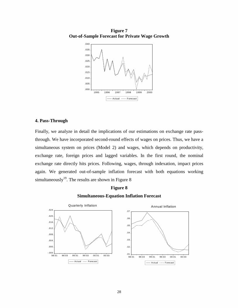
Figure 7 Out-of-Sample Forecast for Private Wage Growth

.000

.005

.010

.015

.020

.025

.030

.035

.040

1995 1996 1997 1998 1999 2000

Actual Forecast

4. Pass-Through

Finally, we analyze in detail the implications of our estimations on exchange rate pass-

through. We have incorporated second-round effects of wages on prices. Thus, we have a

simultaneous system on prices (Model 2) and wages, which depends on productivity,

exchange rate, foreign prices and lagged variables. In the first round, the nominal

exchange rate directly hits prices. Following, wages, through indexation, impact prices

again. We generated out-of-sample inflation forecast with both equations working

simultaneously19. The results are shown in Figure 8

Figure 8

Simultaneous-Equation Inflation Forecast

-.004

.000

.004

.008

.012

.016

.020

.024

98:01 98:03 99:01 99:03 00:01 00:03

Actual Forecast

.01

.02

.03

.04

.05

.06

.07

98:01 98:03 99:01 99:03 00:01 00:03

Actual Forecast

Quarterly Inflation Annual Inflation

29

Figure 9 shows pass-through when the nominal exchange rate increases. First we

incorporated both equations in the García, Herrera and Valdés (2000) five-equation

model –instead of their Phillips curve. Next, given that this model does not have money,

ie it is a real model, we hit both real and equilibrium-real exchange rate with a 10%

shock. After that we observed the nominal exchange rate and price paths in order to

compute the pass-through effect.

Figure 9 indicates that after a 1% rise in the real exchange rate, the nominal exchange

rate also increases producing an accumulated impact on prices of around 0.14% in the

first two years (8 quarters) which is considered the relevant policy horizon.

Figure 9

0.00

0.02

0.04

0.06

0.08

0.10

0.12

0 2 4 6 8 10 12 14 16 18

Real Exchange Rate

Passthrough

-0.05

0.00

0.05

0.10

0.15

0.20

0.25

0.30

0 2 4 6 8 10 12 14 16 18

Passthrough y-gap

Next, we explore how the effect of an exchange-rate shock depends on economic activity.

Evidence suggests that there is a pass-through decrease when the economy is in a

“recession”. Figure 9 shows what happens in our artificial environment with prices, and

the pass-through effect, if we have a temporary increase of 10% in the exchange rate in

two alternative scenarios. One with the output gap being endogenous and which starts

from zero. The second one has, at the initial point, an exogenous 2 % negative output gap

which fades linearly in 3 years. The inflation effect of depreciation is higher when the

economy is at potential (zero output gap). A negative output gap tends to compensate the

19 This exercise was performed with our restricted price index IPCX2, instead of CPI, affecting wages. We consider that this is the origin of the underestimation of the inflation forecast shown in Figure 8.

30

inflationary effect of depreciation. The negative output gap reduces margins and hence a

fraction of the depreciation is not passed on to consumers20.

Finally, Model 2 in Table 3 suggests that the size of exchange rate pass-through is

positively related to the inflation level. This effect is captured in the variables where the

nominal exchange rate is multiplied by inflation. In both cases the coefficients are

positive and strongly significant. Therefore one could conclude that the low pass-through

from exchange rate to inflation observed in recent years is permanent since inflation has

been stabilized around 3%. It also suggests, as stated above, that inflation overprediction

in the recent past is probably related to miss-measurement of the pass-through

coefficient.

V. Conclusions

Price and wage equations based on a model of imperfect competition were estimated and

used to generate out-of-sample inflation forecast. From the estimations we can conclude:

It is confirmed what was found in previous studies in the sense that output gap and

unemployment have a small impact on inflation due to widespread indexation. Therefore

gradual monetary policy is called for.

Despite the fact that generalized wage indexation is one of the most important elements

explaining price and wage behavior, expectations of future inflation matter. This is a very

important variable to be considered in an inflation-targeting regime, since credibility

could substantially reduce the sacrifice ratio.

We empirically found that productivity reduces unit labor costs and inflation affecting

real wages positively. In addition, a negative relationship between inflation and both

mark-ups and real wages indicates that inflation imposes important costs for firms and

20 This exercise was performed assuming a zero unemployment rate because unemployment was not linked to output gap. Considering this second round effect in this particular exercise would probably generate a lower pass-through.

31

workers. This result emphasizes the benefits of stabilizing the inflation rate. This cost

rises even more when the impact of inflation on real wages is considered.

Finally, the exchange rate pass-through depends positively on economic activity and the

inflation level, explaining why pass-through has been so low in recent years. Therefore

one could conclude that pass-through would be permanently lower than in the nineties

given that inflation has been stabilized around 3%.

32

VII. Bibliography Ball, L. and G. Mankiw, (1995) "Relative-Price Changes as Aggregate Supply Shocks." Quarterly Journal of Economics 110 February: 127-151. Banerjee A. L. Cockerell and B. Russell (2001), “An I(2) Analysis of Inflation and the Markup” Forthcoming Journal of Applied Econometrics. Beaumont, C. V. Cassino and D. Mayes (1994), "Approaches to Modeling Prices at the Reserve Bank of New Zealand," Reserve Bank of New Zealand Discussion Paper No.3. Benabou, R. “Inflation and Markups: Theories and Evidence from the Retail Trade Sector” European Economic Review. Blanchard O. and L. Katz (1997), “What we know an do not know about the natural rate of unemployment” Journal of Economic Perspectives Vol. 11, pages 51-72, winter. Blanchard O. and L. Katz (2001), "Wage Dynamics: Reconciling Theory and Evidence" Mimeo, MIT. Blanchflower D. and A. Oswald (1994), The Wage Curve, The MIT press, Cambridge, Massachusetts. Debelle G. and J. Vickery (1997), "Is the Phillips Curve a Curve? Some Evidence and Implications for Australia," Reserve Bank of Australia Research Discussion Paper No. 9706, October. Doornik, J. And D.F. Hendry (1992), PC-Give version7, “An Interactive Econometric Modeling System,” University of Oxford Press. Dornbusch, R. (1987), “Exchange Rates and Prices,” American Economic Review, vol. 77, No.1, March. Engsted and Haldrup (1999) "Estimating the LQAC Model with I(2) variables" Journal of Applied Econometrics, 14:155-170. García, P., L. Herrera, and R. Valdés (2000) “New Frontiers for Monetary Policy in Chile” Mimeo, Central Bank of Chile. Goldberg, P., and M. Knetter (1997), “Goods Prices and Exchange Rates: What Have We Learned?,” Journal of Economic Literature, Vol. 35, No.3, September. Goldfajn, I., and S. Werlang (2000), “The Pass-through from Depreciation to Inflation: A Panel Study,” Working Paper of the Central Bank of Brazil, July. Haldrup N. (1994), "The Asymptotics of Single-Equation Cointegration Regressions with I(1) and I(2) Variables," Journal of Econometrics 63 pp 153-181.

33

Haldrup N. (1995), "An Econometric Analysis of I(2) Variables," Journal of Economic Surveys Vol.12, No. 5. Harris R. (1995), Using Cointegration Analysis in Econometric Modeling, Chapter 4, Prentice Hall. Haskel, J. C., Martin and I. Small (1995), "Price, Marginal cost and the Business Cycle," Oxford Bulletin of Economics and Statistics, 57, No.1. Inder, B. (1993), "Estimating Long-run Relationships in Economics: a Comparison of Different Approaches," Journal of Econometrics 57, 53-68. Kim, K. (1998), US Inflation and the Dollar Exchange Rate a Vector Error Correction Model," Applied Economics, 30, pp. 613-619. Kim, Y. (1990), "Exchange Rates and Import Prices in the United States: A Varying-Parameter Estimation of Exchange-Rate Pass-Through," Journal of Business & Economic Statistics, Vol. 8, No. 3, July. Kreps, D. and J. Scheinkman (1983), “Quantity Pre-Commitment and Bertrand Competition Yield Cournot Outcomes”, Rand Journal of Economics, vol. 14, pp. 326-337. McCarthy J. (1999), "Pass-Through of Exchange Rates and Import Prices to Domestic Inflation in Some Industrialised Economies," BIS Working Paper No. 79, November. McCallum, B. (1976) "Rational Expectations and the Natural Rate Hypothesis: Some Consistent Estimates," Econometrica, Vol. 44, pp.43-52. Menon, J. (1995), "Exchange Rate Pass-Through" Journal of Economic Surveys Vol. 9, No. 2. Phillips, P. (1986), "Understanding Spurious regressions in econometrics, Journal of Econometrics, 33, 335-346. Phillips P. And M. Loretan (1991), “Estimating Long-run Economic Equilibria” Review of Economic Studies Vol. 58, pp. 407-436. Romer, D, (1996) Advanced Macroeconomics McGraw-Hill Chapters 5 and 6. Rotemberg, J. (1982) “Sticky Prices in the United States.” Journal of Political Economy 60, November. Rotemberg, J. and G. Saloner (1986), “A Supergame Theoretic Model of Price Wars During Booms” American Economic Review, vol. 76, pp. 390-407.

34

Rotemberg, J. and M. Woodford (1991), “Mark-ups and the Business Cycle”, NBER Macroeconomics Annual, 6. Russel, B., Evans, J. and B. Preston (1997), “The impact of Inflation and Uncertainty on the Optimum Price Set by Firms” Department of Economic Studies Discussion Papers, No. 84, University of Dundee. Small, I. (1997), “The Cyclicality of Mark-ups and Profit Margins: Some Evidence for Manufacturing Services,” Working Paper of the Bank of England. Taylor, J. (2000), "Low Inflation, Pass-Through, and the Pricing Power of Firms," Forthcoming European Economic Review Woo W. (1984), "Exchange Rates and the Prices of Nonfood, Non-fuel Products," Brookings Papers on Economic Activity 2.