prestressed pcbt girders made continuous and composite · prestressed pcbt girders made continuous...
TRANSCRIPT

PRESTRESSED PCBT GIRDERS MADE CONTINUOUS AND COMPOSITE
WITH A CAST-IN-PLACE DECK AND DIAPHRAGM
by
Stephanie Koch
Thesis submitted to the faculty of the
Virginia Polytechnic Institute and State University
in partial fulfillment of the requirements for the degree of
MASTER OF SCIENCE
in
CIVIL ENGINEERING
Dr. Carin L. Roberts-Wollmann, Chairperson
Dr. Thomas E. Cousins
Dr. Elisa D. Sotelino
April 22, 2008
Blacksburg, Virginia
Keywords: PCBT Girders, Diaphragm, PCA Method, Restraint Moment
ii
PRESTRESSED PCBT GIRDERS MADE CONTINUOUS AND COMPOSITE
WITH A CAST-IN-PLACE DECK AND DIAPHRAGM
by
Stephanie Koch
ABSTRACT
This research document focuses on prestressed PCBT girders made composite with a
cast-in-place concrete deck and continuous over several spans through the use of continuity
diaphragms. The current design procedure in AASHTO states that a continuity diaphragm is
considered to be fully effective if a compressive stress develops in the bottom of the diaphragm
when the superimposed permanent load, settlement, creep, shrinkage, 50 percent live load, and
temperature gradient are summed, or if the girders are stored at least 90 days when continuity is
established. It is more economical to store girders for fewer days, so it is important to know the
minimum number of days that girders must be stored to satisfy AASHTO requirements.
In 2005, Charles Newhouse developed the positive moment diaphragm reinforcement
detail that is currently being adopted by VDOT. This thesis concludes that Newhouse’s detail,
four No. 6 bars bent 180° and extended into the diaphragm, is adequate for all girders except for
the PCBT-77, PCBT-85, and the PCBT-93 when the girders are stored for a minimum of 90
days. It is recommended that two additional bent strands be extended into the continuity
diaphragm for these three girder sizes.
It was also concluded that about half of the cases result in a significant reduction in the
minimum number of storage days if the designer is willing to perform a detailed analysis. The
other half of the cases must be stored for 90 days because the total moment in the diaphragm will
never become negative and satisfy the AASHTO requirement. In general, narrower girder
spacing and higher concrete compressive strength results in shorter required storage duration.
The PCA Method was used in this analysis with the updated AASHTO LRFD creep, shrinkage,
and prestress loss models. A recommended quick check is to sum the thermal, composite dead
load, and half of the live load restraint moments. The girder must be stored 90 days if that sum is
positive, and a more detailed time-dependent analysis would result in a shorter than 90 day
storage period if that sum is negative.

iii
ACKNOWLEDGEMENTS
I would like to thank Dr. Carin Roberts-Wollmann, the chair of my research committee,
for making the completion of this research possible. Dr. Wollmann has taught me a great deal
through her extensive understanding and unwavering patience in communicating it to me. I also
genuinely appreciate the time and insight that Dr. Tommy Cousins and Dr. Elisa Sotelino have
provided as my committee members.
I am very grateful for the opportunities provided to me by the Charles E. Via, Jr.
Department of Civil and Environmental Engineering. I came to Virginia Tech in the pursuit of a
Master’s degree, but I am leaving with much more than a diploma because of the dedication and
hard work of the exceptional faculty and staff.
I also would like to thank the Via family for their generous donations to the fellowship
which contributed to my financial support. In addition, I would like to thank the Virginia
Transportation Research Council for their continued support of research at Virginia Tech, and in
particular for the funding they provided towards the research of PCBT continuity diaphragms.
It has been a pleasure to work with and develop friendships with so many of the students
and faculty in the Structural Engineering and Materials program. I am thankful that I have had
the opportunity to meet so many talented and kind people while at Virginia Tech.
Also, I also am forever grateful for my family and friends who continue to encourage me
to pursue my dreams. I would especially like to thank my future husband, Ray, who has been
very supportive and has helped to make the past two challenging years a wonderful experience. I
am also thankful for my parents, Ken and Kay, who have always provided me with ample love,
encouragement, and guidance. Thanks also to Michelle, Bradley, and Charles who have always
been able to balance the right amount of laughter and sincerity. I would not be where I am today
without the love and encouragement of my family and friends.
Finally, I would like to thank God for all of the blessings in my life. Only through Him is
all of this made possible.

iv
TABLE OF CONTENTS
ABSTRACT.................................................................................................................................... ii
ACKNOWLEDGEMENTS........................................................................................................... iii
LIST OF FIGURES ...................................................................................................................... vii
LIST OF TABLES....................................................................................................................... viii
CHAPTER 1: INTRODUCTION................................................................................................... 1
1.1 Continuity Diaphragms in Composite Systems .................................................................. 1
1.2 AASHTO LRFD Bridge Design Specifications ................................................................. 4
1.3 Research Objectives............................................................................................................ 5
1.4 Thesis Organization ............................................................................................................ 8
CHAPTER 2: LITERATURE REVIEW........................................................................................ 9
2.1 Continuous Prestressed Concrete Girder Bridge Systems .................................................. 9
2.1.1 History........................................................................................................................ 9
2.1.2 Continuity Diaphragm Reinforcement..................................................................... 10
2.2 Time-dependent Effects in Prestressed Concrete ............................................................. 11
2.2.1 Concrete Shrinkage.................................................................................................. 12
2.2.2 Concrete Creep......................................................................................................... 14
2.2.3 Relaxation of Prestressing Steel............................................................................... 18
2.3 Analysis Methods for Creep and Shrinkage ..................................................................... 19
2.3.1 Principle of Superposition........................................................................................ 19
2.3.2 Effective Modulus Method ...................................................................................... 19
2.3.3 Rate of Creep Method.............................................................................................. 21
2.3.4 Rate of Flow Method ............................................................................................... 22
2.3.5 Improved Dischinger Method .................................................................................. 22
2.3.6 Age Adjusted Effective Modulus Method ............................................................... 22
2.4 Design Procedures for Continuity Diaphragms ................................................................ 23
2.4.1 PCA Method ............................................................................................................ 23
2.4.2 NCHRP 322 Method................................................................................................ 26
2.5 Thermal Effects................................................................................................................. 27
2.5.1 Background .............................................................................................................. 28
v
2.5.2 AASHTO LRFD Specifications .............................................................................. 29
2.6 Summary of Need for Research........................................................................................ 30
CHAPTER 3: TESTING THE PCA METHOD........................................................................... 31
3.1 Problem Description ......................................................................................................... 31
3.2 Separate Sections Method................................................................................................. 32
3.2.1 Calculation of Change in Stresses Using the Separate Sections Method ................ 34
3.2.2 Calculation of Rotation Using the Separate Sections Method................................. 36
3.3 PCA Method ..................................................................................................................... 37
3.3.1 Calculation of Change in Stresses Using the PCA Method..................................... 38
3.3.2 Calculation of Rotation Using the PCA method...................................................... 40
3.4 Prestress Applied to Composite Cross-Section ................................................................ 42
3.5 Set-Up and Results............................................................................................................ 43
3.5.1 Comparison of Stresses............................................................................................ 43
3.5.2 A Better Creep Coefficient ...................................................................................... 44
3.6 Conclusions....................................................................................................................... 50
CHAPTER 4: GIRDERS OLDER THAN 90 DAYS................................................................... 51
4.1 Background and Calculations ........................................................................................... 51
4.1.1 Design Variables and Assumptions ......................................................................... 52
4.1.2 Calculations.............................................................................................................. 52
4.1.3 Sample Calculations................................................................................................. 56
4.2 Results............................................................................................................................... 56
4.3 Conclusions....................................................................................................................... 58
CHAPTER 5: GIRDERS YOUNGER THAN 90 DAYS ............................................................ 60
5.1 Introduction....................................................................................................................... 60
5.2 Models............................................................................................................................... 60
5.2.1 AASHTO Creep Model ........................................................................................... 61
5.2.2 AASHTO Shrinkage Model..................................................................................... 62
5.2.3 AASHTO Prestress Loss Model .............................................................................. 63
5.2.4 QConBridge ............................................................................................................. 63
5.2.5 Thermal Moment ..................................................................................................... 64
5.3 Calculations....................................................................................................................... 66

vi
5.3.1 Cases Analyzed........................................................................................................ 66
5.3.2 MathCAD Spreadsheet ............................................................................................ 67
5.4 Results............................................................................................................................... 68
5.4.1 Interpreting Results .................................................................................................. 69
5.4.2 All Results................................................................................................................ 70
5.4.3 General Trends......................................................................................................... 72
5.4.3.1 Changes in Length .......................................................................................... 72
5.4.3.2 Changes in Compressive Strength .................................................................. 72
5.4.3.3 Changes in Girder Spacing ............................................................................. 72
5.4.4 Two-Span vs. Three-Span........................................................................................ 74
5.5 Conclusions....................................................................................................................... 75
CHAPTER 6: CONCLUSIONS AND RECOMMENDATIONS................................................ 77
6.1 Conclusions and Recommendations ................................................................................. 77
6.1.1 Testing the PCA Method ......................................................................................... 77
6.1.2 Girders Older than 90 Days ..................................................................................... 77
6.1.3 Girders Younger than 90 Days ................................................................................ 78
6.2 Recommendations for Future Work.................................................................................. 79
REFERENCES ............................................................................................................................. 81
APPENDIX A: Design of Continuity Diaphragms for Girders Older than 90 Days ................... 83
APPENDIX B: Strands for PCBT Girder Older than 90 Days..................................................... 86
APPENDIX C: 2-Span PCBT Girder Systems Younger than 90 Days........................................ 91
APPENDIX D: 3-Span PCBT Girder Systems Younger than 90 Days ..................................... 128
APPENDIX E: PCBT Details and Section Properties................................................................ 130

vii
LIST OF FIGURES
Figure 1.1: Simple Continuity Diaphragm Illustration................................................................... 1
Figure 1.2: Strains and Stress in a Composite Section ................................................................... 2
Figure 1.3: Restraint Moment Illustration ...................................................................................... 3
Figure 1.4: Charles Newhouse’s Continuity Diaphragm Detail ..................................................... 7
Figure 2.1: Shrinkage Strain over Time........................................................................................ 13
Figure 2.2: Strain Diagram for Creep ........................................................................................... 15
Figure 2.3: Superposition of Creep Strains................................................................................... 16
Figure 2.4: Prestress Loss over time ............................................................................................. 18
Figure 2.5: Effective Modulus ...................................................................................................... 20
Figure 2.6: Positive Temperature Gradient through Cross-Section.............................................. 29
Figure 3.1: Forces, Moments, and Strain Distribution for a Composite Cross-Section ............... 32
Figure 3.2: Change in Stress Distribution through Cross-Section................................................ 35
Figure 3.3: Sample of Change in Curvature along Half of the Span Length................................ 37
Figure 3.4: Stress through Cross-Section if Creep is Zero .......................................................... 38
Figure 3.5: Stress through Cross-Section if Creep is Infinite ...................................................... 38
Figure 3.6: Change in Stress through Cross-Section (from Zero to Infinite Creep).................... 39
Figure 3.7: M/EI Diagram for Straight Strands ............................................................................ 41
Figure 3.8: M/EI Diagram for Harped Strands ............................................................................. 42
Figure 3.9: Percent Difference between PCA Phi and the Best Fit Phi........................................ 50
Figure 4.1: Sketch of PCBT Girder with Deck and Haunch......................................................... 51
Figure 4.2: Length of Prestressing Strand Extended into the Continuity Diaphragm .................. 54
Figure 4.3: Cracking Moment and Design Strength for PCBT-45 Girder.................................... 57
Figure 5.1: Thermal Forces in PCBT Girders............................................................................... 65
Figure 5.2: Restraint Moment ....................................................................................................... 66
Figure 5.3: Continuity Diaphragm Restraint Moments ................................................................ 69
viii
LIST OF TABLES
Table 3.1: Sample Given Parameters for Testing the PCA Method ............................................. 35
Table 3.2: Design Parameters from Newhouse............................................................................. 42
Table 3.3: Sample Stresses (ksi) using the Separate Section Method .......................................... 45
Table 3.4: Sample Stresses (ksi) using the PCA Method ............................................................. 45
Table 3.5: Percent Difference of Stresses for a Girder and Deck Phi of 2.00 .............................. 46
Table 3.6: Percent Difference of Stresses for a Girder and Deck Phi of 1.75 and 2.25 ............... 48
Table 3.7: Comparison of PCA Phi to Best Fit Phi ...................................................................... 49
Table 4.1: Bent Strands Required and Recommended for PCBT Girders.................................... 58
Table 5.1: Experimental Results, PCBT-29 to PCBT 53.............................................................. 70
Table 5.2: Experimental Results, PCBT-61 to PCBT 93.............................................................. 71
Table 5.3: Three-Span Systems vs. Two-Span Systems: Minimum Storage Duration ................ 75

1
CHAPTER 1: INTRODUCTION
1.1 Continuity Diaphragms in Composite Systems
The amount of pressure on the United States transportation infrastructure continues to
increase as our growing population demands new roads and older roadways need to be replaced.
Only a portion of the necessary funds are available for building new bridges and replacing
deficient ones, so unfortunately there are always additional projects that are not considered a
high enough priority. Therefore, research in bridge design is crucial. High quality structures
need to be designed and built with increasing efficiency to allow them to better serve society for
a longer period of time while leaving finances for other undertakings. This research document
focuses on one specific type of bridge system: precast prestressed concrete girders made
composite with a cast-in-place concrete deck and made continuous over several spans through
the use of continuity diaphragms. This type of bridge system was selected because it has many
advantages.
A composite bridge system is one in which the deck and the girders are bonded together
so that the system strains and deflects as one unit. Figure 1.1 is a simple illustration of a
continuity diaphragm with a cast-in-place deck. Composite construction is generally preferred
because there is a substantial increase in strength and stiffness when the deck and girders are tied
together. However, it is more difficult to calculate the forces in the system due to time-
dependent effects, especially in the case of precast prestressed concrete girders with a cast-in-
place deck.
Figure 1.1: Simple Continuity Diaphragm Illustration
Girder Girder
Deck
Continuity
Diaphragm
Deck
Pier

2
The time-dependent effects that occur in the girders and deck include creep, shrinkage,
and relaxation of prestressing steel. It is found that the most dominant forces and moments
develop from differential shrinkage between the deck and girder, which occurs because each
component has a different ultimate value and rate of creep and shrinkage. Nevertheless, the
entire cross-section must strain compatibly since the girders and the deck are made composite
when the deck is poured. In other words, compression develops in the top of the girder and
tension develops in the bottom of the deck since there cannot be discontinuity in the strain
through the cross-section of the girder and deck. See Figure 1.2 for illustration. These forces
will cause rotation at the end of the girder if it is simply supported, and restraint moments will
develop in the continuity diaphragm if the bridge is made continuous.
Figure 1.2: Strains and Stress in a Composite Section
A continuous bridge is one in which two or more simple spans are connected end-to-end
with continuity diaphragms (see Figure 1.1). To understand the moments that develop in a
continuity diaphragm, consider a simply supported system. The ends of the girder are able to
rotate freely throughout the service life of the bridge from the effects of creep, shrinkage,
prestress loss, live loads, temperature gradients, and other loading conditions. In a continuous
system, no further end rotation is allowed after the continuity diaphragm is poured and the ends
of the girders are fixed. Restraint moments must then develop in the continuity diaphragm to
oppose those moments that would rotate the end of the girder if it were unrestrained. See Figure
1.3
Deck
Girder
Cross-Section Unrestrained
Strains
Restrained
Strains
Resulting
Stresses

3
Restraint
Moment
Figure 1.3: Restraint Moment Illustration
A continuous bridge has several advantages over a series of simple span structures. First,
there is a reduction in mid-span bending moments and deflections. This is economical because
the girder cross-section can be reduced, or fewer prestressing strands can be used in cases where
the member size is fixed (Mattock, et al. 1960). Secondly, making a bridge continuous will
improve serviceability by eliminating joints in the deck. The removal of joints will improve the
riding surface of the bridge, and durability will be increased because the water and salts from the
deck will not drain onto the substructure. Many people consider this the most important
advantage (Freyermuth 1969). In addition, the exclusion of joints in a design will reduce the
initial cost of the bridge and also reduce bridge maintenance. Third, a bridge that has been made
continuous will redistribute moments if the load capacity is exceeded for a particular girder in
the system (Mattock, et al. 1960). This provides redundancy.
Although the advantages of continuous systems are numerous and many states are using
them, there is not much agreement on the best method to calculate the restraint moments that
develop in the continuity diaphragms or how to detail the positive moment connection. Note that
the negative moment connection is not discussed in this document because it is provided through
the deck reinforcement, which is much easier to adjust than the positive moment reinforcement
that must enter into the end of the girder. This study uses the current design standards, which are
the AASHTO LRFD Bridge Design Specifications, for the analysis of the positive moment
connection in continuity diaphragms (AASHTO 2007).

4
1.2 AASHTO LRFD Bridge Design Specifications
The Virginia Department of Transportation (VDOT) has been designing an increasing
number of continuous bridges using the relatively new Precast Concrete Bulb Tee (PCBT)
girders. The primary goal of this research is to determine if the continuity diaphragms in bridges
using PCBT girders are in compliance with current LRFD Specifications. Section 5.14.1.4.5 in
the AASHTO LRFD Bridge Design Specifications states:
“The connection between precast girders at a continuity diaphragm shall
be considered fully effective if either of the following are satisfied:
• The calculated stress at the bottom of the continuity diaphragm for
the combination of superimposed permanent load, settlement,
creep, shrinkage, 50 percent live load and temperature gradient, if
applicable, is compressive.
• The contract documents require that the age of the precast girders
shall be at least 90 days when continuity is established and the
design simplifications of Article 5.14.1.4.4 are used.
Section 5.14.1.4.4 states:
“ The following simplification may be applied if acceptable to the owner
and if the contract documents require a minimum girder age of at least 90
days when continuity is established:
• Positive restraint moments caused by girder creep and shrinkage
and deck slab shrinkage may be taken to be 0.
• Computation of restraint moments shall not be required.
• A positive moment connection shall be provided with a factored
resistance, ФMn, not less than 1.2 Mcr, as specified in Article
5.12.1.4.9.”
So, the AASHTO Specifications are straightforward and relatively simple as long as the
girders are older than 90 days before they are made composite and continuous. However, since it
is less economical to wait until girders are 90 days old, it is preferable to store them for less than
5
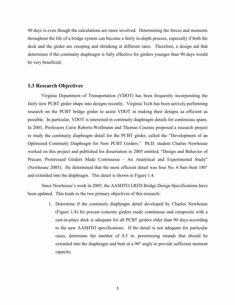
90 days is even though the calculations are more involved. Determining the forces and moments
throughout the life of a bridge system can become a fairly in-depth process, especially if both the
deck and the girder are creeping and shrinking at different rates. Therefore, a design aid that
determines if the continuity diaphragm is fully effective for girders younger than 90 days would
be very beneficial.
1.3 Research Objectives
Virginia Department of Transportation (VDOT) has been frequently incorporating the
fairly new PCBT girder shape into designs recently. Virginia Tech has been actively performing
research on the PCBT bridge girder to assist VDOT in making their designs as efficient as
possible. In particular, VDOT is interested in continuity diaphragm details for continuous spans.
In 2001, Professors Carin Roberts-Wollmann and Thomas Cousins proposed a research project
to study the continuity diaphragm detail for the PCBT girder, called the “Development of an
Optimized Continuity Diaphragm for New PCBT Girders.” Ph.D. student Charles Newhouse
worked on this project and published his dissertation in 2005 entitled, “Design and Behavior of
Precast, Prestressed Girders Made Continuous – An Analytical and Experimental Study”
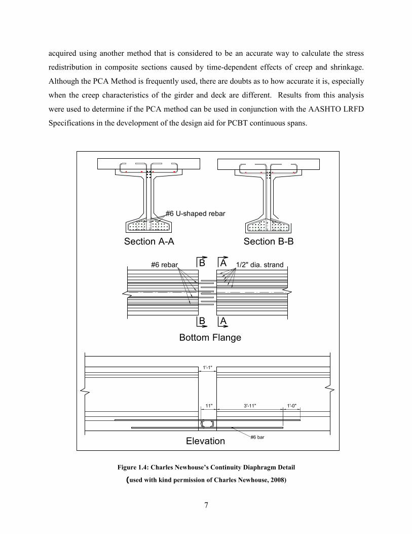
(Newhouse 2005). He determined that the most efficient detail was four No. 6 bars bent 180°
and extended into the diaphragm. This detail is shown in Figure 1.4.
Since Newhouse’s work in 2005, the AASHTO LRFD Bridge Design Specifications have
been updated. This leads to the two primary objectives of this research:
1. Determine if the continuity diaphragm detail developed by Charles Newhouse
(Figure 1.4) for precast concrete girders made continuous and composite with a
cast-in-place deck is adequate for all PCBT girders older than 90 days according
to the new AASHTO specifications. If the detail is not adequate for particular
cases, determine the number of 0.5 in. prestressing strands that should be
extended into the diaphragm and bent at a 90° angle to provide sufficient moment
capacity.
6
2. Determine the minimum number of days that a particular PCBT girder in a
continuous and composite system must age before being erected so that the new
AASHTO specifications are satisfied.
To satisfy the first objective of this research, design parameters were varied to determine
if the Newhouse diaphragm detail for PCBT girders is sufficient for all cases. The assumptions
include:
• The bridge being analyzed is a two-span continuous structure
• The diaphragm concrete has a compressive strength of 4 ksi
• The deck thickness is 8 in.
• The haunch height is 1 in.
• The yield strength of the reinforcing bars is 60 ksi.
A two-span continuous system is more critical than a three or more span system, and the other
assumptions are typical for VDOT designs. The variable parameters include the beam spacing,
the span length and the beam size. For each size girder, the design strength (ФMn) must be
greater than or equal to 1.2 times the cracking moment for multiple combinations of girder
spacings and span lengths. If this requirement is not met, additional 0.5 in. prestressing strands
are extended into the diaphragm to satisfy the requirement.
To meet the second objective of this research, it is necessary to develop a design aid (in
the form of a MathCAD spreadsheet) that will determine when continuity diaphragms for PCBT
girder bridges can be assumed to be fully effective according to Article 5.12.1.4.5 of the
AASHTO specifications. A variety of different size PCBT girders at different ages, span
lengths, compressive concrete strengths, and deck widths were considered in this study. The
design aid simplifies the current procedure and allows for continuous brides to be designed and
built more efficiently. This will save time and money in the design and construction processes.
Another component of the second objective is to explore how accurately the PCA
Method calculates stresses and strains in composite concrete sections. This is important because
the PCA Method is very commonly used and accepted for calculating the restraint moment due
to time-dependent effects. Results obtained using the PCA Method are compared to those results
7
acquired using another method that is considered to be an accurate way to calculate the stress
redistribution in composite sections caused by time-dependent effects of creep and shrinkage.
Although the PCA Method is frequently used, there are doubts as to how accurate it is, especially
when the creep characteristics of the girder and deck are different. Results from this analysis
were used to determine if the PCA method can be used in conjunction with the AASHTO LRFD
Specifications in the development of the design aid for PCBT continuous spans.
Elevation
1'-1"
11" 3'-11" 1'-0"
#6 bar
Bottom Flange
1/2" dia. strand#6 rebar AB
AB
Section A-A Section B-B
#6 U-shaped rebar
Figure 1.4: Charles Newhouse’s Continuity Diaphragm Detail
(used with kind permission of Charles Newhouse, 2008)
8
1.4 Thesis Organization
This document begins with Chapter 1, the Introduction, which includes a brief summary
of the current design specifications and the research objectives. The relevant background can be
found in the Literature Review in Chapter 2. The analytical investigation and results to
determine if the PCA Method is an accurate method of calculating restraint moments in
continuity diaphragms due to time-dependent effects are found in Chapter 3, Testing the PCA
Method. Chapter 4 presents a discussion, analysis procedure, and conclusions for Girders Older
Than 90 Days. Chapter 5, Girders Younger Than 90 Days, determines the minimum number of
days that prestressed PCBT girders must be stored before being erected so that the AASHTO
LRFD Bridge Design Specifications are met. Finally, the Conclusions and Recommendations
can be found in Chapter 6.
9
CHAPTER 2: LITERATURE REVIEW
2.1 Continuous Prestressed Concrete Girder Bridge Systems
A continuous bridge is one in which two or more simple spans are connected end-to-end
with a continuity diaphragm. Some of the earliest long-span continuous highway bridges built in
the United States were constructed in the early 1960’s and include the Big Sandy River Bridge in
Tennessee and the Los Penasquitos Bridge in California (Freyermuth 1969). After a short trial
period where these aesthetic bridges displayed excellent performance, many states began to
research and design their own continuous bridge systems. Since then, continuous prestressed
concrete girder systems have become a popular choice around the country because of their
numerous advantages. Although people agree on their advantages, there is still much
discrepancy on methods used for design of these systems and the associated reinforcement
details.
2.1.1 History
One of the early methods of making a bridge continuous over two or more spans was to
place the ends of the girders close to each other and post-tension them together. However, this
method was not efficient because the anchorages and tensioning were relatively expensive and
there was considerable friction loss due to the severe curves necessary to make the post-
tensioning effective (Mattock, et al. 1960). Because of these disadvantages, an alternative
method began to develop. The improved method called for leaving a small space between the
ends of the girders and extending positive moment reinforcing steel, instead of post-tensioning
strands, into that region from the beams. Concrete would be added to this section at the time
when the deck was poured to provide continuity over the joint. This area is known as a
continuity diaphragm.
It is important that the continuity diaphragm be fully effective for positive bending
moments. Positive moment occurs in the continuity diaphragm because of creep due to the
prestressing force and thermal effects. The 2005 NCHRP Project 12-53 concluded that cracking
of the diaphragm due to positive bending does not necessarily affect the continuity of the system.
10
It was estimated that continuity was only reduced by 30% when the connection was near failure
(Dimmerling, et al. 2005). However, it is still recommended that full continuity be achieved.
Negative moment occurs in the continuity diaphragm because of differential shrinkage, dead
load creep, loss in prestress, live loads, and superimposed dead load. The negative moment
reinforcement is placed in the deck, and does not need to enter into the end of the girder.
Cracking that develops due to diaphragm moments can present maintenance and aesthetic
problems. Also, it is important to limit cracking over the pier because cracking reduces the
stiffness of the system, which will cause the bridge to behave like a series of simple spans under
large loading events. The resulting increased moment at mid-span could cause failure at a
smaller than expected loading or could reduce the service life of the structure.
2.1.2 Continuity Diaphragm Reinforcement
NCHRP Project 12-53 examined methods of making a positive moment connection for
the portion of a continuous bridge over an interior support (Dimmerling, et al. 2005). Cracking
of the diaphragm reduces the effectiveness of continuity for service loads and also reduces the
ductility of the structure. Positive moment reinforcement will help moderate or eliminate this
cracking. Therefore, it is important to design for the appropriate amount of positive moment so
that the cracking of the diaphragm can be controlled and a significant loss of continuity can be
avoided.
Two basic details that are used for positive moment reinforcement in continuous spans
are compared in NCHRP Project 12-53. Variations of these two details represent the majority of
positive moment reinforcement in continuity diaphragms commonly used in design today. The
first detail consists of prestressing strands that are extended from the end of the girder into the
diaphragm and bent at a 90° angle. The second detail uses mild reinforcing steel that is
embedded into the ends of the girder to be extended into the diaphragm. Experimental testing in
this NCHRP Project concluded that positive moment connections could be made using either of
these methods, although embedding mild reinforcement provided slightly improved connection
capacity over using extended prestressing strands. However, bent bar connections are more
difficult to construct than bent strand connections (Dimmerling, et al. 2005).
11
Charles Newhouse published a study on continuity diaphragms in 2005, part of which
analyzed the performance of various positive moment connections for continuous Precast
Concrete Bulb-Tee (PCBT) girders. The reinforcement details selected for analysis in Charles’
study were similar to those used in the NCHRP Project 12-53. The test specimens included ½ in.
prestressing strands extended from the bottom of the girders and bent at a 90° angle, No. 6 mild
reinforcing bars extended from the bottom of the girders and bent at a 180° angle, and no
reinforcement in the diaphragm. Newhouse concluded that the best design feature was the 180°
hooks of mild reinforcement that extended from the end of the girder into the diaphragm. He
stated that this detail “remained stiffer during the testing and is expected to provide for better
long term connections” (Newhouse 2005).
The Virginia Department of Transportation (VDOT) is in the process of adopting
Newhouse’s recommended continuity diaphragm detail as a design standard. Since the objective
of this research is to develop a design aid for the Virginia Transportation Research Council
(VTRC), this study will only examine Newhouse’s continuity diaphragm standard detail of four
No. 6 “U” shaped pieces of mild reinforcing steel.
2.2 Time-dependent Effects in Prestressed Concrete
Creep and shrinkage of concrete members and relaxation of prestressing strands cause
time-dependent changes in strains in a prestressed bridge system, which result in changes in
stress throughout the cross-section. These stresses can have a large impact, and must be
considered when calculating deformations and the redistribution of forces that occurs (Menn,
1986). Time-dependent effects are defined as those that develop after the hardening of the deck
and continuity diaphragm concrete. There are several causes of time-dependent changes in
strain. These include the creep from girder weight and initial prestressing force, the creep due to
the slab weight, and the differential shrinkage between the girder and the deck (ACI 209R-92).
Nearly all concrete structures are built in stages, and all have time-dependent effects from
creep, shrinkage, and other factors. In many cases, the primary reason to accurately predict time-
dependent losses in prestressed concrete members is to determine prestress loss and the
deflection of the member. In these situations, an elastic analysis of the structure as a whole is
sufficient to approximately determine the forces present. A simple lump sum of losses or a

12
simplified approach may then be used to determine the time-dependent effects at various stages
of construction. It is recommended that losses should be assumed to be between 15 and 20% for
pre-tensioned structures and between 10 and 15% for post-tensioned structures (ACI 209R-92).
However, pronounced time-dependent effects would require analysis at multiple stages of
construction. A more in-depth analysis is needed in continuous and composite construction
where the internal forces at a certain stage of construction are substantially different from those
at another stage. This requires a more accurate estimation of the forces and moments in the
system at multiple times during the construction and service life of the structure.
The time-dependent restraint moments that occur in the continuity diaphragm can
become difficult to compute, especially if prestressed concrete girders are used with a cast-in-
place deck. In general, the negative moments will be caused predominately by differential
shrinkage between the deck and the girder and by the creep of the deck. There will also be
positive moments that will develop due to the creep of the prestressed girders, among others.
The dead load and live load that act on adjacent and remote spans will also have an effect on the
restraint moments that will develop in the continuity diaphragms.
2.2.1 Concrete Shrinkage
Shrinkage is defined as the decrease in the volume of concrete over time. Similarly to
creep, shrinkage occurs rapidly at first, but then at a slower rate as it approaches an asymptote
after a large amount of time (Nilson 1987). Unlike creep, shrinkage is independent of the
loading of the concrete. This makes computation simpler because shrinkage of individual
concrete members will not be affected by different construction sequences. Figure 2.1 illustrates
how shrinkage strain changes over time from an initial time, t0, to a final time, t.

13
Figure 2.1: Shrinkage Strain over Time
The three main types of shrinkage are autogenous shrinkage, carbonation shrinkage, and
drying shrinkage. First to be discussed is autogenous shrinkage, which occurs because the
physical materials in concrete take up less space after hydration (MacGregor, et al. 2005). It
does not include any type of moisture exchange between the member and the environment, and is
also known as basic shrinkage or chemical shrinkage (ACI 209R-05). Second is carbonation
shrinkage, which is when water and carbon dioxide mix with the calcium hydroxide in the
cement paste to produce calcium carbonate and additional water. This process of reducing the
volume of the cement only occurs if the humidity is not too high or too low, because moisture is
needed for the reaction but too much will restrict the reaction. Finally, drying shrinkage occurs
when moisture is allowed to enter and leave the member, and is the focus of most research at this
time. It occurs because water slowly moves to the surface of the concrete and is lost due to
evaporation, so the other particles become more compact (MacGregor, et al. 2005). For the
duration of this study, the term “shrinkage” will refer solely to “drying shrinkage.” This is
because researchers commonly assume that all of the shrinkage strain is due to drying shrinkage
for normal weight concrete, while the contributions from autogenous and carbonation shrinkage
can be neglected (ACI 209R-05).
Differential shrinkage occurs between two pieces of concrete if they must strain together
but have different rates of shrinkage. An example of this is a prestressed girder with cast-in-
place deck, because shrinkage occurs at different rates if both are allowed to shrink separately
(Mattock, et al. 1961). They have different shrinkage rates because they are cast with different
types of concrete and the concrete in the deck is younger. In this case where the deck is made
composite with the girder, new forces and moments are introduced since there still must be a
constant change in strain throughout the entire cross-section. Since the girder with a composite
Shrinkage Strain, εsh
to t Time
Strain

14
deck would deflect downward if a simple span were being analyzed, the corresponding rotations
at the end of the girder would result in a negative restraint moment in a continuity diaphragm.
There are several factors in the mix design that influence shrinkage rates and the ultimate
value of shrinkage strain. Aggregates restrain shrinkage, so the volume of aggregates in the
concrete is often considered to be the most important factor limiting shrinkage (ACI 209R-05).
Likewise, stiffer and larger aggregate results in less shrinkage because the concrete is better
restrained (MacGregor, et al. 2005). Increasing water content will cause more shrinkage because
the total volume of the aggregates must be reduced (ACI 209R-05). For similar reasons,
shrinkage will increase when there is a greater ratio of the volume of cement to the volume of
concrete (MacGregor, et al. 2005). The type of cement will also influence shrinkage, with those
having more finely ground cement or low quantities of sulfate exhibiting more shrinkage (ACI
209R-05).
The ambient environment during the life of the member also influences shrinkage, so the
curing process and the duration of the drying period will have an effect. For example, steam
curing can significantly reduce shrinkage by as much as 30%, and extended periods of moist
curing can reduce shrinkage by 10 to 20% (ACI 209R-05). Humidity at the construction site will
also affect shrinkage, with low humidity causing increased shrinkage. Temperature also affects
shrinkage, but the effects are minimal when compared to humidity (MacGregor, et al. 2005).
Finally, the size and shape of a member will also influence shrinkage. This is because
shrinkage will occur more slowly when moisture has to travel through more material to reach the
air (ACI 209R-05). In other words, a very long and slender member would shrink more than a
short compact one, if all other factors were the same. A volume-to-surface-area ratio is often
computed to measure this geometric property, and assists in calculations of shrinkage. The
relationship that is defined by the ACI 209 committee states that shrinkage is considered to be
inversely proportional to the square of the volume-to-surface-area ratio (MacGregor, et al. 2005).
2.2.2 Concrete Creep
Creep is defined as the deformation of concrete under sustained loading, or an increase of
strain under constant stress. In other words, constant stress in a member will not result in

15
constant strain because creep will cause the member to increasingly deform throughout time.
Creep causes strain to increase quickly at first, but then it will increase at a slower rate as it
approaches an asymptote (Nilson 1987).
Consider a sustained load that is applied to a member. Instantaneous elastic strains occur
in the member at the time the load is applied, to, and then creep strains develop slowly over time
as the load is sustained. Figure 2.2 illustrates this example.
Figure 2.2: Strain Diagram for Creep
The process of calculating the strain due to creep becomes more complicated if there is
more than one applied load. This is because concrete becomes increasingly stiff as it ages; in
other words, the modulus of elasticity increases over time. Figure 2.3 depicts multiple loadings
on a specimen.
Creep Strain, εcp
Elastic Strain, εo
εcp(t,to)
εo(t,to)
ε(t,to)
to t
Strain
Time
16
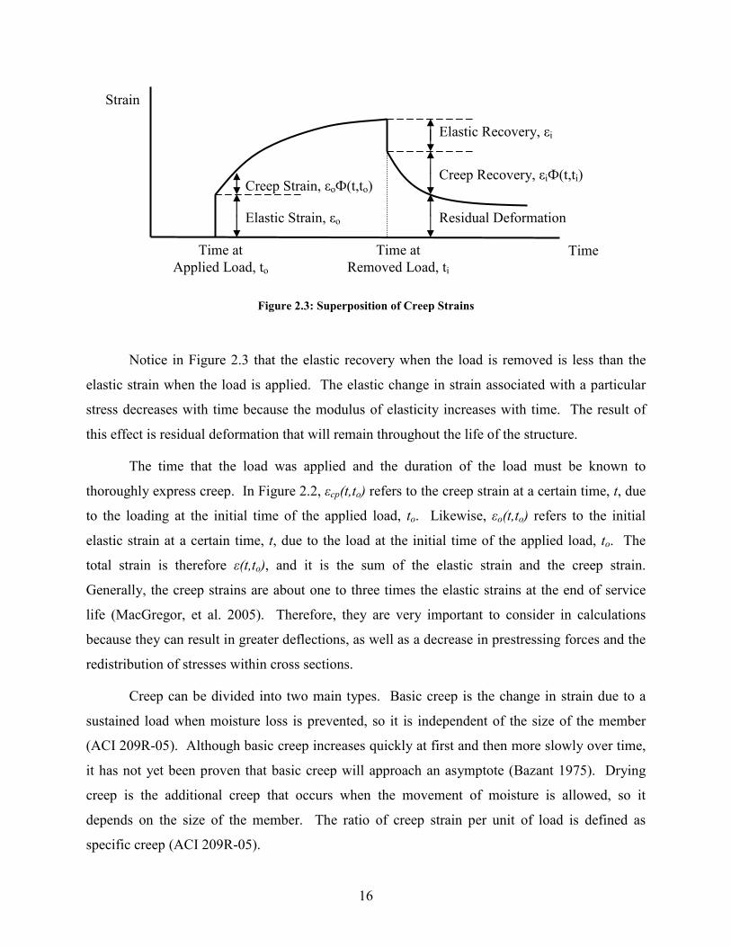
Figure 2.3: Superposition of Creep Strains
Notice in Figure 2.3 that the elastic recovery when the load is removed is less than the
elastic strain when the load is applied. The elastic change in strain associated with a particular
stress decreases with time because the modulus of elasticity increases with time. The result of
this effect is residual deformation that will remain throughout the life of the structure.
The time that the load was applied and the duration of the load must be known to
thoroughly express creep. In Figure 2.2, εcp(t,to) refers to the creep strain at a certain time, t, due
to the loading at the initial time of the applied load, to. Likewise, εo(t,to) refers to the initial
elastic strain at a certain time, t, due to the load at the initial time of the applied load, to. The
total strain is therefore ε(t,to), and it is the sum of the elastic strain and the creep strain.
Generally, the creep strains are about one to three times the elastic strains at the end of service
life (MacGregor, et al. 2005). Therefore, they are very important to consider in calculations
because they can result in greater deflections, as well as a decrease in prestressing forces and the
redistribution of stresses within cross sections.
Creep can be divided into two main types. Basic creep is the change in strain due to a
sustained load when moisture loss is prevented, so it is independent of the size of the member
(ACI 209R-05). Although basic creep increases quickly at first and then more slowly over time,
it has not yet been proven that basic creep will approach an asymptote (Bazant 1975). Drying
creep is the additional creep that occurs when the movement of moisture is allowed, so it
depends on the size of the member. The ratio of creep strain per unit of load is defined as
specific creep (ACI 209R-05).
Time at
Applied Load, to
Strain
Time
Elastic Strain, εo
Time at
Removed Load, ti
Residual Deformation
Elastic Recovery, εi
Creep Strain, εoФ(t,to) Creep Recovery, εiФ(t,ti)
17
Some of the factors that influence the creep of concrete include the mix design, curing
process, humidity, temperature, and age of concrete when loaded (MacGregor, et al. 2005). One
of the most important is the mix design, which includes the quantity of aggregate, size of
aggregate, elastic properties of the aggregate, water content, air content, and cement content.
Creep will generally be greater when the aggregate volume is smaller, the aggregate has lower
elastic properties, the water content is higher, and the air content is higher. The cement content
and the size of the aggregate do cause variations in creep, but it is difficult to determine their
definitive effects. Another important factor is the surrounding environment, which affects the
drying creep of a concrete member. The ambient relative humidity and temperature will cause
greater creep if they encourage the evaporation of moisture from the specimen (ACI 209R-05).
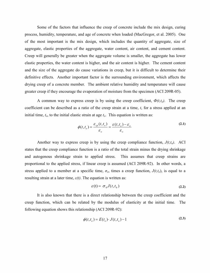
A common way to express creep is by using the creep coefficient, Ф(t,to). The creep
coefficient can be described as a ratio of the creep strain at a time, t, for a stress applied at an
initial time, to, to the initial elastic strain at age to. This equation is written as:
(2.1)
Another way to express creep is by using the creep compliance function, J(t,to). ACI
states that the creep compliance function is a ratio of the total strain minus the drying shrinkage
and autogenous shrinkage strain to applied stress. This assumes that creep strains are
proportional to the applied stress, if linear creep is assumed (ACI 209R-92). In other words, a
stress applied to a member at a specific time, σo, times a creep function, J(t,to), is equal to a
resulting strain at a later time, ε(t). The equation is written as:
(2.2)
It is also known that there is a direct relationship between the creep coefficient and the
creep function, which can be related by the modulus of elasticity at the initial time. The
following equation shows this relationship (ACI 209R-92):
(2.3)
o
oo
o
ocp
o
tttttt
εεε
ε
εφ
−==
),(),(),(
)(= 00 , (t) ttJσε
1),()(),( −⋅= ooo ttJtEttφ
18
2.2.3 Relaxation of Prestressing Steel
A concrete member is put into compression when the prestressing tendons are cut or
when the post-tensioning strands are stressed. This tensile force keeps the member uncracked
for a longer period of time, which results in additional stiffness. However, there are both
instantaneous and time-dependent losses that cause a reduction in the prestressing force.
The immediate loss that occurs in a pre-tensioned member is due to the elastic shortening
of the concrete, although it is assumed that the change in length of the member is negligible for
computational purposes. If a member is post-tensioned, the instantaneous losses would also
include the friction between the tendons and the duct and the anchorage slip when the jacking
force is transferred to the member (Nilson 1987). Since these elastic losses occur immediately
after the transfer of compression to the member, they will not have long term effects on the
system. However, there is creep that will occur in the girder because of this prestressing force.
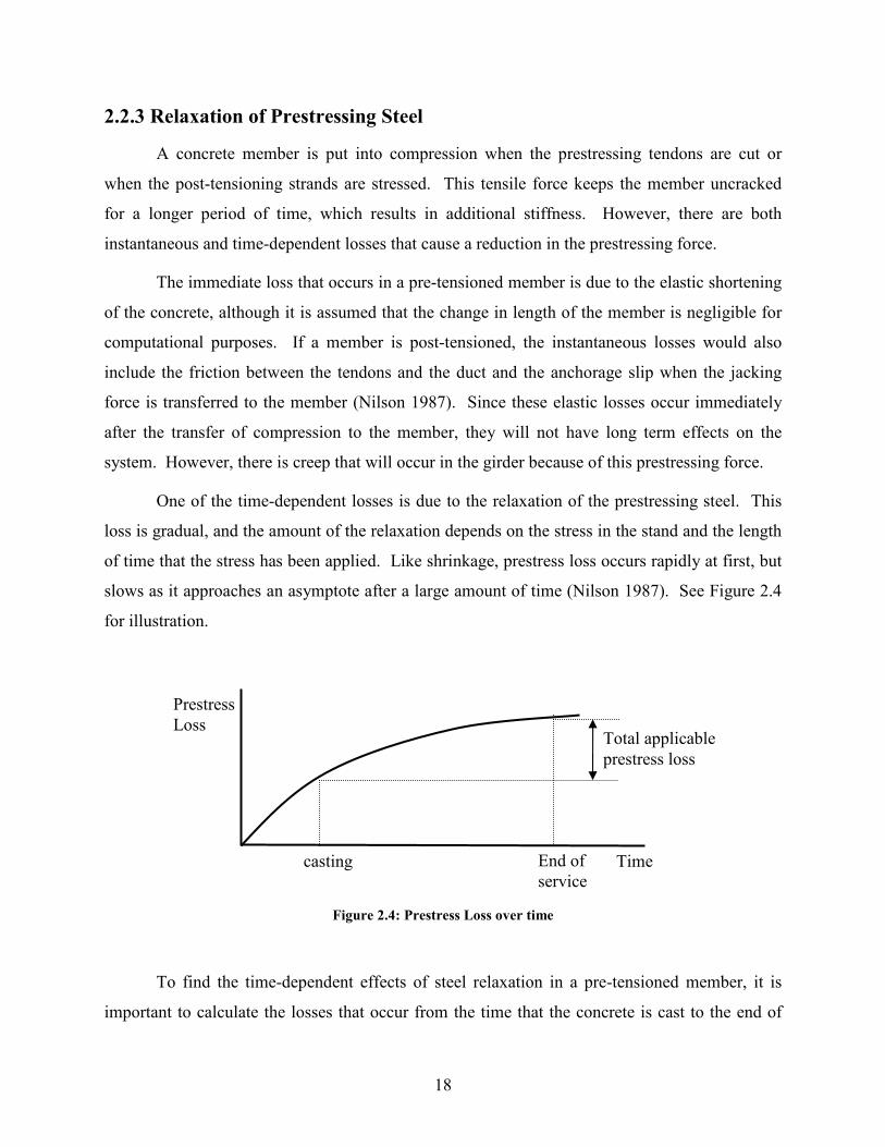
One of the time-dependent losses is due to the relaxation of the prestressing steel. This
loss is gradual, and the amount of the relaxation depends on the stress in the stand and the length
of time that the stress has been applied. Like shrinkage, prestress loss occurs rapidly at first, but
slows as it approaches an asymptote after a large amount of time (Nilson 1987). See Figure 2.4
for illustration.
Figure 2.4: Prestress Loss over time
To find the time-dependent effects of steel relaxation in a pre-tensioned member, it is
important to calculate the losses that occur from the time that the concrete is cast to the end of
casting End of
service
Time
Prestress
Loss Total applicable
prestress loss
19
service life. This is found by subtracting the losses that occur from the initial time of
prestressing to the time when the concrete is cast from the losses that occur from the initial time
of prestressing to the end of service life.
2.3 Analysis Methods for Creep and Shrinkage
Although the individual properties of creep and shrinkage are fairly well understood,
several different methods have been developed to analyze their behavior over time.
2.3.1 Principle of Superposition
The principle of superposition is an analysis method used to determine the change in
strain from multiple loading and unloading conditions through time. This method determines the
value of creep strain at a particular time due to a load applied at an earlier time. If more than one
load has been applied through the life of the member, all of the creep strain components are then
summed to determine the final creep curve due to all of the loading and unloading cases that
occur at various times. Therefore, this method is fairly straightforward if it is assumed that the
modulus of elasticity of the concrete is constant and if the stress history is well known. A
problem is that this method predicts complete creep recovery, because the modulus of elasticity
is considered to be constant, which is not true.
2.3.2 Effective Modulus Method
The effective modulus method was developed by McMillan (1916) and Farber (1927),
and it is one of the oldest methods to predict the effects of creep (ACI 209R-92). In this method,
the initial modulus of elasticity is adjusted by a factor to account for creep. Figure 2.5 illustrates
this relationship.

20
Figure 2.5: Effective Modulus
In Figure 2.5, the left portion of the x-axis is elastic strain, εo, which occurs at the initial
application of the load. The right portion of the graph is the creep strain, εcr, which occurs under
sustained loading.
As shown in Figure 2.5, the modus of elasticity, E, must change over time since the strain
increases due to creep but stress remains constant. It is known that:
(2.4)
(2.5)
(2.6)
The variable Φ is known as the creep coefficient, and is simply a ratio of the creep strain to the
elastic strain. Setting stress in equations (2.4) and (2.5) equal to each other yields:
(2.7)
(2.8)
σ
E’ E
ε εo, elastic strain εcr, creep strain
0εσ
=E
0
'εε
σ+
=cr
E
o
cr
εε
φ =
)(' croo EE εεε +⋅=⋅
φεεε
+=
+⋅=
1'
EEE
cro
o
21
The effective modulus, E’, is therefore a reduced modulus, which can be used in an
elastic analysis to take into account the effects of creep. This method is simple, but is incorrect
for cases of varying stress. Since the creep strain at a particular time only depends on the current
stress, the stress history is excluded. Also, complete recovery of strain is predicted if the stress is
removed, which is fundamentally incorrect (Mattock, et al. 1961). Therefore, the stress in the
concrete must be fairly constant over the analysis period and the concrete must be older so that
there is not a significant change in the modulus of elasticity in order for this method to be used
(ACI 209R-92).
2.3.3 Rate of Creep Method
Glanville (1930) developed another method to calculate creep, which is known as the rate
of creep method. The basic equation for calculating creep under variable stress using the rate of
creep method is:
(2.9)
where:
T = time
dεc/dT = rate of creep
f = stress
The rate of creep method is based on Glanville’s findings that show that the rate of creep
is independent of the age of the concrete for young members. The method assumes that concrete
will creep at a rate of f*dεc/dT regardless of the stress conditions that occurred in its earlier
history, and therefore the creep coefficient is assumed to be independent of the time of loading
(Mattock, et al. 1961). In other words, all of the forces that are building up with time are
assumed to creep at the same rates as the initially applied load. Since this is not true, this method
is generally considered to be outdated. However, newer methods were developed from the basic
∫=T
c dTdT
dfcreep
0
ε

22
principles of the rate of creep method that accounted for the underestimation of creep and creep
recovery in older members.
2.3.4 Rate of Flow Method
The rate of flow method was developed by England and Illston (1965) to improve the rate
of creep method. They suggested that the creep compliance functions should be the sum of the
elastic strain, the delayed elastic strain, and the irrecoverable flow. The delayed elastic strain
developed much faster than the irrecoverable flow component, so they needed to be separate
components in the formulation of the creep function (ACI 209R-92). The rate of flow method
provided a much needed improvement to the rate of creep method, but it still underestimated the
value of creep under increasing stress.
2.3.5 Improved Dischinger Method
The improved Dischinger method was formulated when Nielsen (1970) tried to further
advance the development of the creep function by combining the rate of creep and the rate of
flow methods. He proposed that the irrecoverable flow should be treated similarly as the total
creep in the rate of creep method. This method was presented in the CEB-FIP Model Code in
1978 after Rusch, Jungwirth, and Hilsdorf (1973) provided additional modifications.
2.3.6 Age Adjusted Effective Modulus Method
Another method was developed by Trost (1967) and later modified by Bazant (1972)
which is today known as the Age Adjusted Effective Modulus method. This method improves
upon the previously discussed effective modulus method by making use of an aging coefficient
(ACI 209R-92). When a load is applied at a time after the initial loading, an adjustment to the
ultimate value of creep is needed because the concrete ages. So, the effective modulus, E’, must
be further modified to the age-adjusted effective modulus, E’’. It can be found by:
(2.10)
χφ+
=1
''E
E

23
In equation (2.10), χ is the age-adjusted factor or the aging coefficient which accounts for
changes with time because creep occurs at a slower rate as a member continues to age. The
aging coefficient can only be used if the support conditions change instantaneously or if the
support conditions change at approximately the same rate as creep, which is the case for
shrinkage (ACI 209R-92). In other words, the aging coefficient can be used as long as support
conditions do not change considerably faster or slower than creep.
The aging coefficient has a value between 0.5 and 1.0. If the concrete does not age, as in
the case of an old member loaded for a short amount of time, the aging coefficient is almost 1.0.
On the other hand, if a young member is loaded for a very long period of time, the aging
coefficient is nearly 0.5 (Jirsasek 2002). It is recommended that an aging coefficient of 0.8 be
used for most analyses (Dilger 1983, Bazant 2002). The Age Adjusted Effective Modulus
method is a method that is commonly used in analysis and design of concrete structures today.
In 1982, Dilger published his work on creep-transformed section properties to help
analyze members with steel reinforcement. Previously, all of the steel would be combined into
one layer for calculations, which would produce inaccurate results. This was a widespread
problem since many prestressed structures have more than one layer of steel. This method states
that unrestrained creep, free shrinkage, and reduced inherent relaxation should be applied to the
creep-transformed cross-section (ACI 209R-92). This study ignores the steel reinforcement,
since it is minimal in comparison to the amount of concrete present.
2.4 Design Procedures for Continuity Diaphragms
There currently are several design procedures that calculate the restraint moment in a
continuity diaphragm. These include the PCA Method (Freyermuth 1969) and the National
Cooperative Highway Research Program (NCHRP) 322 Method (Oesterle, et al. 1989).
2.4.1 PCA Method
In the 1950’s the Portland Cement Association (PCA) undertook several projects that
focused on composite construction so that an analysis method could be developed (Hongestad, et
al. 1960). The findings of a well-known researcher, Mattock, were also included in the

24
development of the PCA Method which states, “the effects of creep under prestress and dead
load can be evaluated by an elastic analysis assuming that the girder and slab were cast and
prestressed as a monolithic continuous girder” (Mattock, et al. 1961). The result was the
“Design of Continuous Highway Bridges with Precast Prestressed Girders” bulletin (Freyermuth
1969), which laid out the PCA Method that is still used in the calculation of restraint moments in
continuity diaphragms today.
The article published by Freyermuth (1969) stated that the effects of the prestressing
force and dead load can be modified to account for creep by multiplying by a factor of:
(2.11)
The negative restraint moment due to shrinkage can be modified by a factor of:
(2.12)
The PCA Method also outlined a method to calculate the creep coefficient. The specific
creep strain for a loading that occurs at a girder age of 28 days is based on the modulus of
elasticity at the time of the loading. This modulus is obtained from a 20-year loading curve,
assuming that the ultimate creep occurs at 20 years. Another figure is then used to adjust the
creep strain for the actual age of the concrete at loading, which occurs when the girder is
prestressed. A size coefficient is used to adjust the creep strain for a particular volume to
surface-area ratio that is being analyzed. Since this method is used to analyze composite and
continuous systems, another figure is used to determine the coefficient that represents the percent
of the ultimate creep that will have occurred at the time the connection is made. The creep
strain that must be developed by the continuity diaphragm must therefore be adjusted by a factor
of 100 percent minus the percent of creep strain that has occurred up to the time of continuity.
The creep coefficient, Ф, for the creep strain that is remaining can be found by the following:
(2.13)
(2.14)
(2.15)
φ−− e1
φ
φ−− e1
elastic
creep
ε
εφ =
elastic
Eε1
=
Ecreep ⋅= εφ

25
where:
εcreep = creep strain
εelastic = elastic strain
E = initial modulus of elasticity
The PCA Method also defined the differential shrinkage moment due to the different
shrinkage rates of the girder and the deck. It can be applied to the girder along its entire length:
(2.16)
(2.17)
(2.18)
where:
εdiff = differential shrinkage strain
Eb = elastic modulus for the deck slab concrete
Ab = cross-sectional area of deck slab
e’2 = centroid of the composite section
t = thickness of the slab
εs = shrinkage strain at any time, T
εsu = ultimate shrinkage strain
V/S = volume to surface-area ratio
The 1969 PCA bulletin contained an equation to calculate the time-dependent restraint
moment over the pier. It is:
(2.19)
+⋅⋅⋅=2
'2t
eAEM bbdiffs ε
TN
T
s
sus +
⋅=ε
ε
SV
s eN/36.0
0.26⋅⋅=
LLsDLcr Ye
YeYYM +
−⋅−−⋅−=
−−
φ
φφ 1)1()(

26
where:
Mr = final restraint moment
Yc = restraint moment at a pier due to creep under prestress force
YDL = restraint moment at a pier due to creep under dead load
Ys = restraint moment at a pier due to differential shrinkage between the slab and girder
YLL = positive live load plus impact moment
PCA bulletin also recommended positive and negative moment reinforcement. It was
decided that a viable option for the positive moment continuity reinforcement was reinforcing
bars at right angles that were extended into the diaphragm. This detail was tested, and it is
recommended that 60% of the yield stress should be used in design of the diaphragm so that the
live load plus impact stress range is reduced and there is more assurance against the possibility of
diaphragm cracking. It was also suggested that the negative moment continuity reinforcement be
designed using the compressive strength of the girder concrete. This bulletin notes that the
shear provisions in the AASHTO Specifications of Highway Bridges provide a conservative
estimate of the shear capacity of the beams in a continuous system, but the formulas must be
applied over the full length instead of only over the middle half of the spans.
The second part of the article published by Freyermuth in 1969 included design
examples. The first was for a bridge with four continuous spans with an arbitrary length. The
next model expanded on the details of the first example, and spans of 130 ft were selected for the
Type IV AASHTO girders.
2.4.2 NCHRP 322 Method
By the early 1980’s, continuous bridge design had changed considerably since the PCA
Method was developed and implemented. Bridges could span larger distances and have a girder
spacing that was greater. Also, the material properties of concrete were changing along with the
methods of analysis to model the behavior of these structures. Therefore, although the bridges
27
that were designed using the PCA Method seemed to be performing fairly well, a new method
was sought that would predict the behavior of these structures more accurately.
In the 1980’s the National Cooperative Highway Research Program (NCHRP) performed
a study to develop procedures for the computation of design moments in the continuity
diaphragms of prestressed bride girders. It was known as NCHRP Project 12-29, and the
objectives were to investigate the positive and negative moments to be used in the design of the
connections in precast prestressed bridge girders made continuous. The work completed
included several experimental investigations involving creep and shrinkage that were performed
in Skokie, Illinois, and several analytical investigations of typical continuous bridges.
The NCHRP 322 report summarized and explained the findings of NCHRP Project 12-
29. The report noted that the time-dependent effects and the construction sequences must be
considered for design. Suggested combinations of girder age at time of deck and diaphragm
placement, and age of girder at live load moments, were also included. In addition, computer
programs that calculate the service moments using the NCHRP 322 method were developed to
aid designers.
2.5 Thermal Effects
Temperature is an important factor influencing creep and shrinkage of a concrete
structure. For example, tests have shown that creep strains are approximately two to three times
greater for specimens at 122°F, compared to those at 68 to 75°F (Manual of Concrete Practice).
Changes in the average temperature of the structure can occur throughout the entire cross-section
of the bridge. This will result in translational distortions if the bridge is free to expand and
contract, while stresses are introduced if the superstructure is restrained. Also, temperature
variations can exist through the cross-section of the bridge. Temperature gradients will cause
rotational distortions if the bridge is unrestrained, and bending moments in bridges that are
continuous. It is important to be able to model and analyze the effects of temperature gradients
on a continuous concrete structure because the bending moments that are introduced must be
included in the restraint moment that develops in the continuity diaphragm.
28
2.5.1 Background
Heat can be transferred by radiation, convection, and conduction. Usually the
contributions from convection and conduction are so small that a single coefficient will consider
these effects (Imbsen, et al. 1985). Heat transfer by radiation occurs when the structure is
exposed to sunlight, and often results in noticeable thermal changes.
Temperature gradients occur because the top and bottom of a member are exposed to a
change in temperature and absorb heat rapidly, while the middle portion is predominately
insulated from these effects due to the relatively non-conductive nature of concrete. A positive
thermal gradient is one in which the deck is warmer than the girder, and a negative thermal
gradient is one in which the deck is cooler than the girder. A maximum positive thermal gradient
would occur on a sunny and warm day after a few days of cool overcast weather. Likewise, a
negative temperature gradient may be applicable on a cool day following warm weather.
Thermal gradients in structures were often not considered before 1980. Then, even after
the importance of accounting for temperature changes was universally recognized, there were
many different opinions on how to quantify them to predict the best responses. Although
thermal effects were known to introduce some additional strain in the cross-section of a bridge,
there were not many reported cases where temperature caused significant damage (Imbsen, et al.
1985). Researchers now attribute this to the slightly conservative nature of the design process.
Also, the effects of temperature were often largely overlooked, even in situations where
temperature was cited as being a likely reason for cracking, because it was known that creep and
shrinkage also contributed to the problem.
Engineers realized that bridge design in the United States could be slightly simplified if a
standard temperature gradient could be agreed upon and modified to account for geographically
specific thermal conditions. In 1978, the British Standard BS 5400 published results defining a
negative thermal gradient. This gradient was adopted by the 1985 NCHRP Report 276 as the
standard negative thermal gradient for use in the United States. In 1983, a study was published
by Potgieter and Gamble that outlined a positive thermal gradient to be used in the design of
typical US bridges (Potgieter, et al. 1983). This gradient was based on data gathered from
weather stations around the country. This was the positive thermal gradient that was adopted by
the 1985 NCHRP Report 276 (Imbsen, et al. 1985) as the standard for use.
29
The NCHRP Report 276 was very important because at that time states considered the
effects of axial length changes to be the most severe, and no state included temperature gradient
effects in its typical design codes. In this report, field tests and meteorological data were
compiled to divide the United States into four zones for solar radiation (Imbsen, et al. 1985).
This temperature gradient was later modified and introduced into the AASHTO LRFD Bridge
Design Specifications and is further discussed in Section 2.5.2.
Although a standard temperature gradient is used in continuity diaphragm calculations
today, thermal effects are still being researched. A series of experimental tests were completed
in 2005 as part of the NCHRP Project 12-53 to examine the performance of diaphragm
reinforcement common in the United States. It was concluded that daily temperature changes
affect the end reactions in a continuous system by as much as 25%, which reinforced the
importance of including thermal effects in the design of continuity diaphragms (Dimmerling, et
al. 2005).
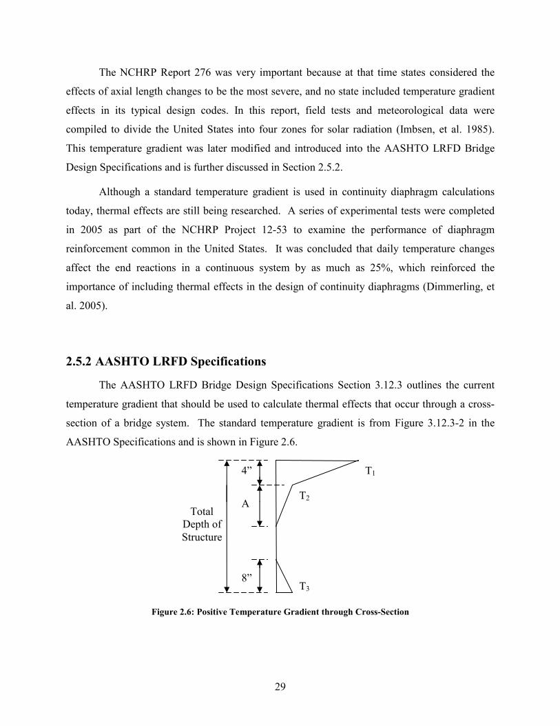
2.5.2 AASHTO LRFD Specifications
The AASHTO LRFD Bridge Design Specifications Section 3.12.3 outlines the current
temperature gradient that should be used to calculate thermal effects that occur through a cross-
section of a bridge system. The standard temperature gradient is from Figure 3.12.3-2 in the
AASHTO Specifications and is shown in Figure 2.6.
Figure 2.6: Positive Temperature Gradient through Cross-Section
T1
T2
T3
4”
A
8”
Total
Depth of
Structure
30
As stated in Section 2.5.1, the United States is divided into 4 zones based on climate.
From Figure 3.12.3-1 in the AASHTO Specifications, it is obtained that Virginia is in Zone 3.
Table 3.12.3-1 in AASHTO Specification shows that the temperatures associated with Zone 3
are:
T1 = 41°F
T2 = 11°F
Section 3.12.3 in AASHTO states that T3 should be taken as 0°F unless a site study indicates
otherwise, and the maximum value that can be used for T3 is 5°F. For the analysis in this
project, T3 will be taken to be 0°F since no other data is available. Section 3.12.3 also defines
the value of the dimension A in Figure 2.6 as 12.0 in. for concrete superstructures that have a
depth of 16 in. or more. All of the PCBT girders, which are the types that will be considered in
this study, fall into this category.
2.6 Summary of Need for Research
First, the PCA Method is often considered to be fairly accurate and conservative in the
calculation of time-dependent restraint moments that develop in continuity diaphragms. Since
the basis of this method was developed by Mattock in the early 1960’s, it would be beneficial to
confirm that the PCA Method is still accurate for bridges with modern properties.
Secondly, it is important to further analyze the continuity diaphragm detail developed by
Charles Newhouse. It must be checked that the detail is adequate for all PCBT girders that are
stored for 90 days according to the new AASHTO specifications.
Finally, it would be advantageous to develop a design aid that assists in the calculation of
time-dependent restraint moments for girders that are stored for less than 90 day according the
new AASHTO specifications. Although previous research studies discuss the time-dependent
moments that develop in continuity diaphragms of concrete bridge systems, one does not exist
that calculates the restraint moments for PCBT girders according to new code requirements.

31
CHAPTER 3: TESTING THE PCA METHOD
3.1 Problem Description
The time-dependent restraint moment that develops in a continuity diaphragm includes
the differential shrinkage restraint moment, the prestress losses restraint moment, the moment to
restrain prestress creep rotations, and the moment to restrain dead load creep rotations. The PCA
Method (Equation 2.19) is a widely accepted method used to calculate the restraint moment due
to time-dependent effects. It is often preferred because it is relatively simple and considered to
be conservative.
The work of Alan Mattock is the basis for what is known as the PCA Method today
(Mattock, et al. 1961). He states that moments develop to restrain the end rotation that would
have occurred if the girders in continuous spans were not rigidly connected. Mattock concluded
from his research that these moments, “are similar in character and distribution to the secondary
moments which are set up in monolithic prestressed continuous girders, prestressed by a non-
concordant prestressing tendon”. He also concluded that, “for design purposes, and assuming
usual construction procedures, it may be assumed that the distribution of moments and forces
will change toward that which would have occurred if the loads applied to the individual
elements before continuity was established had instead been applied to the structure after
continuity was established” (Mattock, et al. 1961). Mattock assumes that the creep coefficients
of the girder and deck are the same, but problems arise because that is not the case for most real
bridge structures. Also, it has been debated if the prestress force should be applied to the girder
alone instead of the composite cross-section as Mattock suggests. Therefore, there are two
questions that needed to be answered before the PCA Method was used in the calculation of
prestress restraint moments for this research:
1. Should the prestress moment be applied only to the girder or to the composite cross-
section?
2. Does the PCA Method accurately predict the restraint moment in continuity
diaphragms if the creep coefficients for the girder and the deck are different?
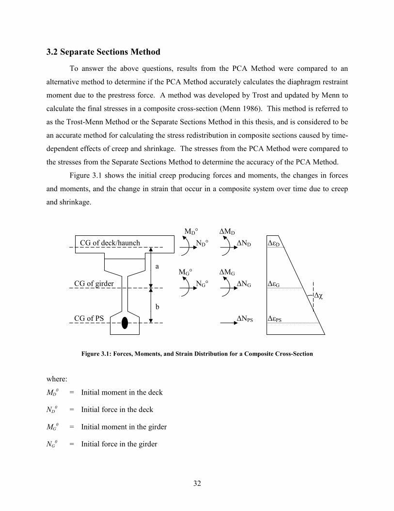
32
3.2 Separate Sections Method
To answer the above questions, results from the PCA Method were compared to an
alternative method to determine if the PCA Method accurately calculates the diaphragm restraint
moment due to the prestress force. A method was developed by Trost and updated by Menn to
calculate the final stresses in a composite cross-section (Menn 1986). This method is referred to
as the Trost-Menn Method or the Separate Sections Method in this thesis, and is considered to be
an accurate method for calculating the stress redistribution in composite sections caused by time-
dependent effects of creep and shrinkage. The stresses from the PCA Method were compared to
the stresses from the Separate Sections Method to determine the accuracy of the PCA Method.
Figure 3.1 shows the initial creep producing forces and moments, the changes in forces
and moments, and the change in strain that occur in a composite system over time due to creep
and shrinkage.
Figure 3.1: Forces, Moments, and Strain Distribution for a Composite Cross-Section
where:
MD0 = Initial moment in the deck
ND0 = Initial force in the deck
MG0 = Initial moment in the girder
NG0 = Initial force in the girder
CG of girder
∆MD
∆ND
∆MG
∆NG
∆NPS
∆εD
∆εG
∆εPS
∆χ
CG of PS
CG of deck/haunch
b
a
MD°
ND°
MG°
NG°
33
∆MD = Change in the moment in the deck
∆ND = Change in the force in the deck
∆MG = Change in the moment in the girder
∆NG = Change in the force in the girder
∆NPS = Change in the force in the deck
∆εD = Change in strain in the deck
∆εG = Change in strain in the girder
∆εPS = Change in strain in the prestress
∆χ = Change in curvature of the system
a = Distance from centroid of the deck and haunch to the centroid of the girder
b = Distance from the centroid of the girder to centroid of prestress
The separate sections method is based on the equations of internal equilibrium, the
equations relating forces to deformations in the girder and the deck (constitutive equations), and
compatibility of deformations through the depth of the cross-sections using the above listed
variables. It is assumed that all changes in moments and forces are positive, so a negative
change in force resulting from the solution of the simultaneous equations denotes a more
compressive force. The equations are shown below:
Equilibrium:
(3.1)
(3.2)
Constitutive:
(3.3)
0=∆+∆+∆ PSGD NNN
0=∆+∆+∆⋅+∆⋅ GDPSD MMNbNa
)1( D
DD
DD
DD
o
DD
AE
N
AE
Nφµφε ⋅+
∆+=∆
34
(3.4)
(3.5)
(3.6)
(3.7)
Compatibility:
(3.8)
(3.9)
After the equations are derived, they can be solved simultaneously. Tensile stresses and
elongating strains are considered to be positive, while moments and curvatures with compression
at the top and tension at the bottom are positive. The initial forces and moments are considered
to be known parameters because they are found from the initial loads on the section. Solving
the system of equations gives the changes in the forces, moments, and strains in the system.
Note that shrinkage was ignored for this study. Also notice that the prestress relaxation is not
included in this analysis because it is considered to be negligible compared to the other forces.
3.2.1 Calculation of Change in Stresses Using the Separate Sections Method
Equations (3.1) through (3.9) are solved simultaneously so the stress distribution changes
can be determined for the cross-section. Consider an example of a PCBT 77 girder with a span
length of 130 ft, girder spacing of 6 ft, 38 prestressing strands, and a creep coefficient of 2.0 for
the girder and deck. The given parameters at mid-span are found in Table 3.1. The stress
distribution for this example at mid-span, found using the Separate Sections Method, is shown in
Figure 3.2. Note that tension is considered to be positive. The first term in Equation 2.19
calculates the creep due to the quantity of the prestressing minus dead load times the reduction
)1( G
GG
G
G
GG
o
G
GAE
N
AE
Nφµφε ⋅+
∆+=∆
psps
ps
psEA
N
⋅
∆=∆ε
aGD ⋅∆−∆=∆ χεε
bGPS ⋅∆+∆=∆ χεε
)1( G
GG
G
G
GG
o
G
IE
M
IE
Mφµφχ ⋅+
∆+=∆
)1( D
DD
DD
DD
o
D
IE
M
IE
Mφµφχ ⋅+
∆+=∆
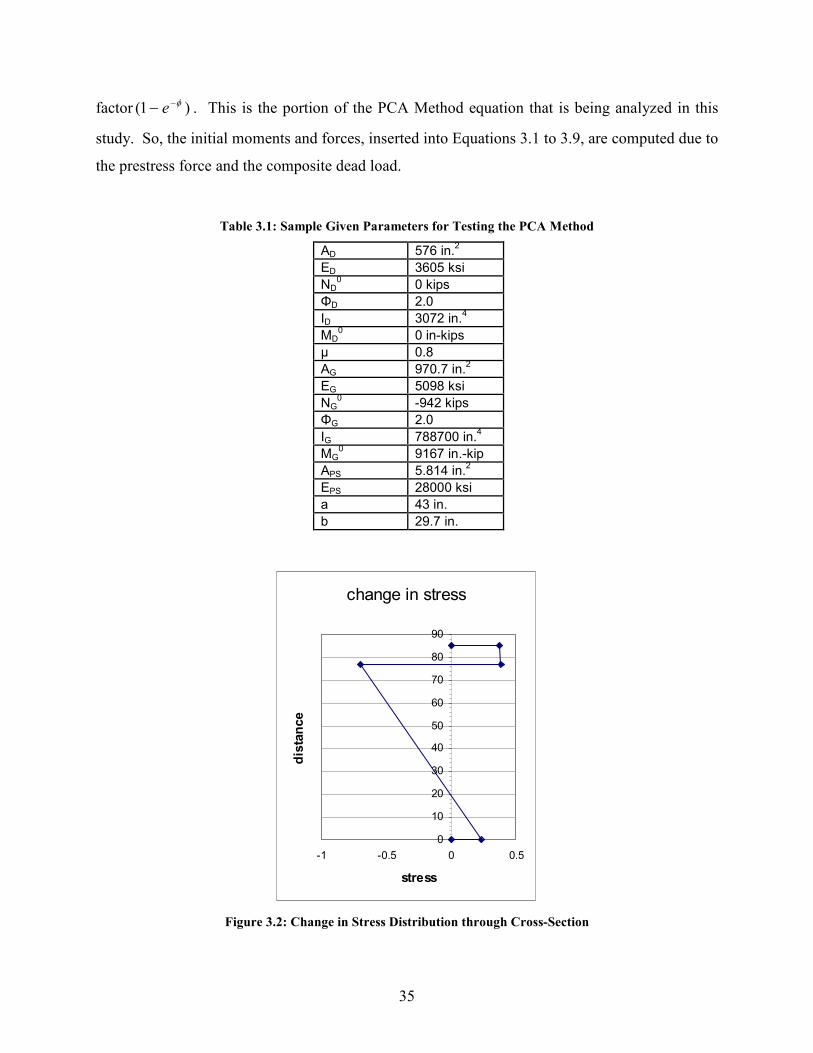
35
factor )1( φ−− e . This is the portion of the PCA Method equation that is being analyzed in this
study. So, the initial moments and forces, inserted into Equations 3.1 to 3.9, are computed due to
the prestress force and the composite dead load.
Table 3.1: Sample Given Parameters for Testing the PCA Method
change in stress
0
10
20
30
40
50
60
70
80
90
-1 -0.5 0 0.5
stress
dis
tan
ce
Figure 3.2: Change in Stress Distribution through Cross-Section
AD 576 in.2
ED 3605 ksi
ND0
0 kips
ΦD 2.0
ID 3072 in.4
MD0
0 in-kips
µ 0.8
AG 970.7 in.2
EG 5098 ksi
NG0
-942 kips
ΦG 2.0
IG 788700 in.4
MG0
9167 in.-kip
APS 5.814 in.2
EPS 28000 ksi
a 43 in.
b 29.7 in.

36
3.2.2 Calculation of Rotation Using the Separate Sections Method
The goal of this analysis is to determine if the PCA Method accurately predicts the
restraint moments in continuity diaphragms due to prestressing forces when compared to the
Separate Sections Method. Therefore, it is important to determine if the two methods give
similar rotations at the end of the girder, since the rotation at the ends of the beams is needed to
compute the restraint moments that develop in continuity diaphragms. Note that change in
curvature is defined as the rate of strain change through the depth of a section, while change in
rotation is considered to be the amount that the section rotates (in radians) throughout a given
time. For example, the rotation at an end of a simply supported uniformly loaded beam is found
by summing the area under the curvature diagram over half of the beam.
To estimate the change in rotation, the change in curvature should be obtained for several
critical points. These include the end of the beam, the end of the transfer length, half the
distance to the harping point, the harping point, and mid-span. It is necessary to calculate the
change in rotation at these points, if not more, because the location of the center of gravity of the
strands will cause a variable prestressed moment along the length of the beam and a variable
dead load moment will also be present. The Moment Area Method is used to compute the
change in rotation.
See Figure 3.3 for a general plot of how the change in curvature varies from the support
to mid-span. Note that, for simplicity, it is assumed that there is a linear relationship between
each of these points so that the area under a portion of the curve (and therefore the change in
rotation) can be found by averaging the changes in curvature between points and multiplying by
the distance between them. The total change in rotation at a support is then the total area under
half of the change in curvature diagram, if the beam is symmetric about mid-span. This change in
curvature is then modified by multiplying by )1( φ−− e because the moment will “relax” due to
creep as time progresses.

37
Span Length
Change in Curvature
Figure 3.3: Sample of Change in Curvature along Half of the Span Length
Also, note that a certain distance is needed to develop the prestressing force, which is
known as the transfer length. AASHTO states that testing indicates that the transfer length is
about 50 times the strand diameter. Therefore, the prestressing force, and consequently the
moment caused by the prestressing force, is zero at the end of the beam. It is assumed in our
example, which uses 0.5 in. diameter prestressing strands, that the full prestressing force is
transferred at 25 in. from the end of the beam.
3.3 PCA Method
As previously mentioned, the PCA Method only considers the creep coefficient of the
girder. This allows stresses and strains to be computed directly, which avoids the complicated
simultaneous equations necessary in the Separate Sections Method. Stresses and strains are
computed and compared to the results from the Separate Sections Method. This example is
again for a PCBT 77 girder with a span of 130 ft, girder spacing of 6 ft, 38 strands, and creep
coefficient of 2.0 for the girder and deck that was discussed in Section 3.2.1.
mid span
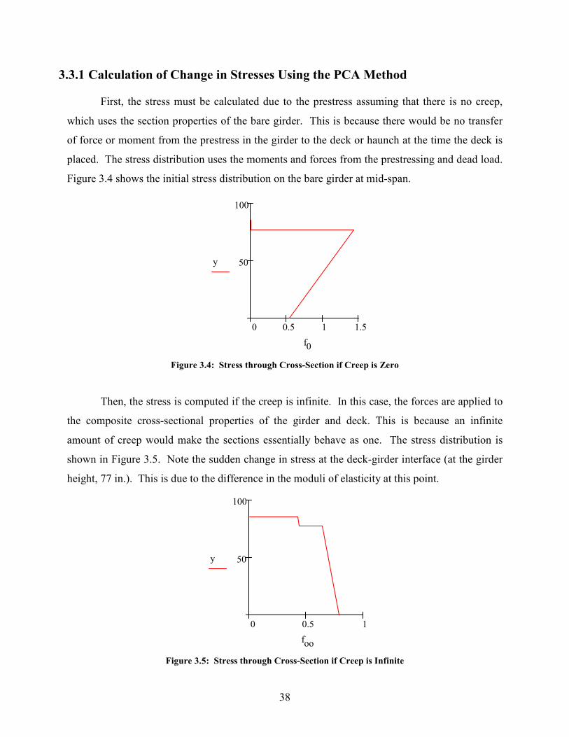
38
3.3.1 Calculation of Change in Stresses Using the PCA Method
First, the stress must be calculated due to the prestress assuming that there is no creep,
which uses the section properties of the bare girder. This is because there would be no transfer
of force or moment from the prestress in the girder to the deck or haunch at the time the deck is
placed. The stress distribution uses the moments and forces from the prestressing and dead load.
Figure 3.4 shows the initial stress distribution on the bare girder at mid-span.
0 0.5 1 1.5
50
100
y
f0
Figure 3.4: Stress through Cross-Section if Creep is Zero
Then, the stress is computed if the creep is infinite. In this case, the forces are applied to
the composite cross-sectional properties of the girder and deck. This is because an infinite
amount of creep would make the sections essentially behave as one. The stress distribution is
shown in Figure 3.5. Note the sudden change in stress at the deck-girder interface (at the girder
height, 77 in.). This is due to the difference in the moduli of elasticity at this point.
0 0.5 1
50
100
y
foo
Figure 3.5: Stress through Cross-Section if Creep is Infinite

39
Subtracting the stress when creep is infinite from the stress when there is no creep will
yield the change in stress due to creep. This is shown in Figure 3.6.
1 0.5 0 0.5
50
100
y
fc
Figure 3.6: Change in Stress through Cross-Section (from Zero to Infinite Creep)
Then, the final stress for the top of the deck, bottom of the deck, top of the girder, and
bottom of the girder can be found using the relationships defined in the PCA Method. They are:
(3.10)
(3.11)
(3.12)
(3.13)
where:
ftg,f = stress in the top of the girder at final time
ftg,o = stress in the top of the girder at no creep
ftg,c = change in stress in the top of the girder from no creep to infinite creep
Фg = creep coefficient of the girder
The other variables in Equations (3.11) to (3.13) are defined similarly to those in Equation (3.10)
for the bottom of the deck, the top of the girder, and the bottom of the girder. Note that
differential shrinkage is ignored.
( )gctdotdftd efff φ−−⋅+= 1,,,
( )gcbdobdfbd efff φ−−⋅+= 1,,,
( )gctgotgftg efff φ−−⋅+= 1,,,
( )gcbgobgfbg efff φ−−⋅+= 1,,,

40
3.3.2 Calculation of Rotation Using the PCA Method
Using the initial stresses and the change in stresses, the following equations were used to
compute the change in curvature:
(3.14)
(3.15)
(3.16)
where:
∆εgt = change in strain at the top of the girder
Фg = creep coefficient of the girder
Eg = modulus of elasticity of the girder
ftg,o = initial stress at the top of the girder
ftg,c = change in stress at the top of the girder
∆εbt = change in strain in the bottom of the girder
fbg,o = initial stress at the bottom of the girder
fbg,c = change in stress at the bottom of the girder
∆χ = change in curvature
h = height of the girder
Equations (3.13) through (3.15) were computed at mid-span, and were compared to the
change in curvature at mid-span using the Separate Sections Method. As mentioned previously,
it is important to compare the unrestrained rotation at the end of the beams since that will cause
diaphragm restraint moments to develop in continuous spans. The PCA Method states that the
rotation at the end of the beam can be computed using the following equations:
( 3.17)
( )ctgotg
g
g
gt ffE
,, +=∆φ
ε
( )cbgobg
g
g
bt ffE
,, +=∆φ
ε
h
bgtg εεχ
∆−∆=∆
( )compg
scompeffs
sIE
LeyPSpca
⋅⋅
⋅−⋅⋅=
2θ

41
( 3.18)
( 3.19)
where:
θpcas = rotation due to straight strands
θpcah = rotation due to harped strands
θpca = total rotation
Ss = number of straight strands
Sh = number of harped strands
Peff = effective prestressing force per strand
ycomp = composite centroid measured from the bottom of the girder
es = centroid of straight prestressing strands measured from the bottom of the girder
ehms = centroid of harped prestressing strands from the bottom of the girder at mid-span
ehend = centroid of harped prestressing strands from the bottom of the girder at end of beam
L = span length
Eg = modulus of elasticity of the girder
Icomp = composite moment of inertia
Note that one of the objectives of Chapter 3 is to determine if θpca should involve the centroid of
the bare beam instead of the composite centroid. See Section 3.4 for this discussion. Also,
notice that Equations (3.17) and (3.18) are derived using the Moment Area Method, so the M/EI
diagrams for straight and harped strands are shown in Figure 3.7 and Figure 3.8.
Figure 3.7: M/EI Diagram for Straight Strands
L 0.5L
Pe/EI
( ) ( )[ ]compg
compendmscompeffh
hIE
LyehehyPSpca
⋅
⋅−−−⋅=
⋅ 2.01.0θ
hs pcapcapca θθθ +=

42
Figure 3.8: M/EI Diagram for Harped Strands
3.4 Prestress Applied to Composite Cross-Section
A brief study is needed to show if the prestress force should be applied to the composite
cross-section as recommended by the PCA Method. The prestress was the only loading
condition considered in this study, and shrinkage was ignored. The work of Charles Newhouse
(Newhouse 2005) contains a design example which can be used to compare the PCA Method and
the Separate Sections Method. The parameters are found in Table 3.2.
Table 3.2: Design Parameters from Newhouse
The updated AASHTO LRFD models for creep, shrinkage, and prestress loss are used in
the time-dependent calculations. The Separate Sections Method gives a rotation of
16,705,478/EI. The rotation using the PCA Method when the prestressing force is applied to the
bare beam is 9,921,428/EI, while the rotation when the PCA Method is used applying the
prestressing force to the composite beam gives a rotation of 16,943,831/EI. See the document
published by Newhouse in 2005 for a more in-depth discussion of the calculations using the
Separate Sections Method.
Girder Size PCBT-45
Girder compressive strength 8 ksi
Span length 100 ft
Modulus of the girder 4578 ksi
Moment of inertia of the girder 207,300 in.4
Distance from girder centroid to the bottom 22.23 in.
Area of the girder 746.7 in.2
Deck width 6 ft
Thickness of the deck 7.5 in.
Haunch thickness 1.5 in.
Composite moment of inertia 432700 in.4
Creep Coefficients (Girder and Deck) 2.0
Pe/EI
0.5L L 0.4L

43
Notice that there is substantially more error when the prestress is applied only to the
girder cross-section. No extensive study was needed because limited results showed very clearly
that applying the prestress to the composite section is more accurate.
3.5 Set-Up and Results
Several trials with a variety of parameters were run to determine if the PCA Method and
the Separate Sections Method gave similar results. It was out of the scope of this document to
analyze all combinations of parameters that could be associated with this problem, so a few were
selected that would provide an overall representation of results. The parameters that were used
include three types of PCBT girders (45, 61, and 77), a deck width of 6 ft and 9 ft, and a long and
medium span length for each case. The suggested number of prestressing strands for each trial
was obtained from the VDOT design guide (see Appendix E).
3.5.1 Comparison of Stresses
The prestressing force was applied to the composite cross-section. The calculated stress
results showed that there was less than 5% error in the calculation of stress at the bottom and top
of the deck and at the bottom and top of the girder for all cases where the creep coefficient of the
girder and the deck were equal. However, there was error introduced when the creep coefficients
were not equal. In general, the greatest percent error occurred in the top of the deck (about 20%
to 25%), and the smallest error occurred in the bottom of the girder (5% or less). The PCA
Method conservatively over-predicted the stress in the bottom of the girder and deck in nearly all
cases, but was not always conservative when predicting the stress in the top of the girder and
deck.
As mentioned in the beginning of section 3.1, the PCA Method is a simplified approach
that assumes the creep coefficients of the girder and the deck are the same and equal to the creep
coefficient of the girder. The results from this study provide reassurance that using the creep
coefficient of the girder was sufficient if the creep coefficients of the girder and the deck were
the same. However, although the PCA Method was almost always conservative, results did vary
if the creep coefficients were different. Since it seems that the creep coefficient of the girder did

44
not provide highly accurate results, an investigation was undertaken to determine if a creep
coefficient can be used in the PCA Method that will more accurately model stresses.
3.5.2 A Better Creep Coefficient
This set of parametric studies addresses if the girder creep coefficient can be modified so
that use in the PCA Method would provide more accurate results in composite systems. It was
quickly determined that an average or a weighted average of the girder and deck creep
coefficients was not the best solution. Using one of these methods increases the creep coefficient
used in the PCA Method because the deck creep coefficient is always greater than or equal to the
girder creep coefficient because the deck concrete is younger than girder concrete. The creep
coefficients that give results closest to those found using the superposition method were less than
the girder creep coefficients.
A parametric study was completed to determine the best creep coefficient to compute
stresses through a cross-section using the cases discussed in Section 3.5, including girder and
deck creep coefficients of 2.00 and 2.00, 1.75 and 2.25, 1.50 and 2.50, 1.25 and 2.75, and 1.00
and 3.00 respectively. Once again, the effects of shrinkage were not included. First, the more
exact stresses were found at several locations through the depth of the composite cross-section
using the Separate Sections Method and the specified creep coefficients. Then, the stresses were
found using the PCA Method and a creep coefficient varying from 2.00 to 0.30 with 0.05
increments. The “best fit” PCA creep coefficient, Φ, was the one that minimized the percent
error for the stresses along the depth of the composite cross-section when compared to those
obtained using the Separate Sections Method.
For example, consider a PCBT 45 girder, with 6 ft girder spacing, a span length of 60 ft,
and 16 prestressing strands. Stresses were calculated using the Separate Sections Method with
numerous values of the girder and deck creep coefficients, and are presented in Table 3.3. The
stresses were then calculated using the PCA Method with varying creep coefficients. For the
above example, the PCA stresses are shown in Table 3.4.

45
Table 3.3: Sample Stresses (ksi) using the Separate Section Method
Фg Фd top deck bottom deck top girder bottom girder
2.0 2.0 0.072 0.119 -0.256 0.655
1.75 2.25 0.067 0.103 -0.281 0.647
1.5 2.5 0.061 0.089 -0.306 0.638
1.25 2.75 0.053 0.074 -0.333 0.628
1.0 3.0 0.045 0.060 -0.362 0.618
Table 3.4: Sample Stresses (ksi) using the PCA Method
PCA Ф top deck bottom deck top girder bottom girder
2.00 0.075 0.123 -0.247 0.658
1.95 0.074 0.122 -0.249 0.657
1.90 0.074 0.121 -0.251 0.656
1.85 0.073 0.120 -0.253 0.655
1.80 0.072 0.119 -0.256 0.655
1.75 0.071 0.117 -0.258 0.654
1.70 0.071 0.116 -0.261 0.653
1.65 0.070 0.115 -0.263 0.652
1.60 0.069 0.113 -0.266 0.651
1.55 0.068 0.112 -0.269 0.650
1.50 0.067 0.110 -0.272 0.649
1.45 0.066 0.109 -0.275 0.648
1.40 0.065 0.107 -0.278 0.647
1.35 0.064 0.105 -0.282 0.645
1.30 0.063 0.103 -0.286 0.644
1.25 0.062 0.101 -0.290 0.643
1.20 0.060 0.099 -0.294 0.641
1.15 0.059 0.097 -0.298 0.640
1.10 0.058 0.095 -0.302 0.638
1.05 0.056 0.092 -0.307 0.636
1.00 0.055 0.090 -0.312 0.635
0.95 0.053 0.087 -0.318 0.633
0.90 0.051 0.084 -0.323 0.631
0.85 0.050 0.081 -0.329 0.629
0.80 0.048 0.078 -0.335 0.627
0.75 0.046 0.075 -0.341 0.624
0.70 0.044 0.072 -0.348 0.622
0.65 0.041 0.068 -0.355 0.619
0.60 0.039 0.064 -0.363 0.617
0.55 0.037 0.060 -0.371 0.614
0.50 0.034 0.056 -0.379 0.611
0.45 0.031 0.052 -0.388 0.608
0.40 0.029 0.047 -0.397 0.605
0.35 0.026 0.042 -0.406 0.601
0.30 0.022 0.037 -0.416 0.598

46
After the stresses are computed using the Separate Sections Method and PCA Method,
they can be compared. See Table 3.5 for percent difference of stresses with the girder and deck
creep coefficients of 2.00.
Table 3.5: Percent Difference of Stresses for a Girder and Deck Phi of 2.00
Фg top deck bottom deck top girder bottom girder
2.00 -4 -3 4 0
1.95 -3 -3 3 0
1.90 -3 -2 2 0
1.85 -1 -1 1 0
1.80 0 0 0 0
1.75 1 2 -1 0
1.70 1 3 -2 0
1.65 3 3 -3 0
1.60 4 5 -4 1
1.55 6 6 -5 1
1.50 7 8 -6 1
1.45 8 8 -7 1
1.40 10 10 -9 1
1.35 11 12 -10 2
1.30 13 13 -12 2
1.25 14 15 -13 2
1.20 17 17 -15 2
1.15 18 18 -16 2
1.10 19 20 -18 3
1.05 22 23 -20 3
1.00 24 24 -22 3
0.95 26 27 -24 3
0.90 29 29 -26 4
0.85 31 32 -29 4
0.80 33 34 -31 4
0.75 36 37 -33 5
0.70 39 39 -36 5
0.65 43 43 -39 5
0.60 46 46 -42 6
0.55 49 50 -45 6
0.50 53 53 -48 7
0.45 57 56 -52 7
0.40 60 61 -55 8
0.35 64 65 -59 8
0.30 69 69 -63 9

47
The percent difference that is shown in Table 3.5 is the difference in stresses calculated
using the PCA and Separate Sections Methods. As shown in Table 3.5 by the highlighted region,
the creep coefficient recommended for use by the PCA Method is 2.00 because the creep
coefficient of the girder is 2.00. However, it is observed in Table 3.5 that a creep coefficient of
about 1.80 should be used in the PCA Method to produce results closest to those obtained using
the more accurate Separate Sections Method. Note that the difference may be due to the aging
coefficient that must be assumed in the Separate Sections Method. A typical value of 0.8 for the
aging coefficient is used in this example.
Likewise, consider girder and deck creep coefficients of 1.75 and 2.25, respectively.
Table 3.6 illustrates the associated percent difference. The creep coefficient used for the PCA
Method is 1.75 because the PCA Method specifies that the creep coefficient of the girder be used
in calculations. However, 1.35 is a more accurate estimation of a creep coefficient that would
give similar results in stress to those obtained using the Separate Sections Method. This more
accurate creep coefficient, Φ, will be regarded as the “best fit Φ” for the remainder of this
document.
This process of determining a creep coefficient that can be used in the PCA Method to
produce stresses closest to those from the Separate Sections Method was repeated for creep
coefficients of the girder and deck of 1.50 and 2.50, 1.25 and 2.75, and 1.00 and 3.00,
respectively. Then, this process was repeated for different girder sizes, span lengths, and girder
spacings, and the results are shown in Table 3.7.
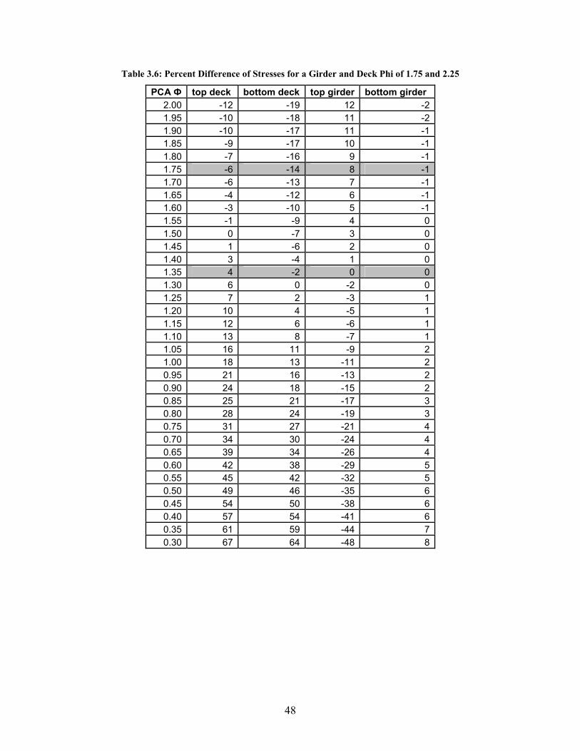
48
Table 3.6: Percent Difference of Stresses for a Girder and Deck Phi of 1.75 and 2.25
PCA Ф top deck bottom deck top girder bottom girder
2.00 -12 -19 12 -2
1.95 -10 -18 11 -2
1.90 -10 -17 11 -1
1.85 -9 -17 10 -1
1.80 -7 -16 9 -1
1.75 -6 -14 8 -1
1.70 -6 -13 7 -1
1.65 -4 -12 6 -1
1.60 -3 -10 5 -1
1.55 -1 -9 4 0
1.50 0 -7 3 0
1.45 1 -6 2 0
1.40 3 -4 1 0
1.35 4 -2 0 0
1.30 6 0 -2 0
1.25 7 2 -3 1
1.20 10 4 -5 1
1.15 12 6 -6 1
1.10 13 8 -7 1
1.05 16 11 -9 2
1.00 18 13 -11 2
0.95 21 16 -13 2
0.90 24 18 -15 2
0.85 25 21 -17 3
0.80 28 24 -19 3
0.75 31 27 -21 4
0.70 34 30 -24 4
0.65 39 34 -26 4
0.60 42 38 -29 5
0.55 45 42 -32 5
0.50 49 46 -35 6
0.45 54 50 -38 6
0.40 57 54 -41 6
0.35 61 59 -44 7
0.30 67 64 -48 8

49
Table 3.7: Comparison of PCA Phi to Best Fit Phi
Girder, span, length Фg, Фd Difference of PCA BestFit Difference in Ф, % Difference of Ф,
Фg & Фd Ф Ф PCA & Best Fit PCA & Best Fit
2.00,2.00 0.0 2.00 1.80 0.200 11
1.75,2.25 0.5 1.75 1.40 0.350 25
1.50,2.50 1.0 1.50 1.05 0.450 43
1.25,2.75 1.5 1.25 0.83 0.420 51
PCBT45,S6,L90
1.00,3.00 2.0 1.00 0.60 0.400 67
2.00,2.00 0.0 2.00 1.80 0.200 11
1.75,2.25 0.5 1.75 1.35 0.400 30
1.50,2.50 1.0 1.50 1.05 0.450 43
1.25,2.75 1.5 1.25 0.80 0.450 56
PCBT45,S6,L60
1.00,3.00 2.0 1.00 0.60 0.400 67
2.00,2.00 0.0 2.00 1.80 0.200 11
1.75,2.25 0.5 1.75 1.43 0.320 22
1.50,2.50 1.0 1.50 1.10 0.400 36
1.25,2.75 1.5 1.25 0.85 0.400 47
PCBT45,S9,L60
1.00,3.00 2.0 1.00 0.62 0.380 61
2.00,2.00 0.0 2.00 1.80 0.200 11
1.75,2.25 0.5 1.75 1.35 0.400 30
1.50,2.50 1.0 1.50 1.03 0.470 46
1.25,2.75 1.5 1.25 0.80 0.450 56
PCBT61,S6,L120
1.00,3.00 2.0 1.00 0.60 0.400 67
2.00,2.00 0.0 2.00 1.80 0.200 11
1.75,2.25 0.5 1.75 1.35 0.400 30
1.50,2.50 1.0 1.50 1.00 0.500 50
1.25,2.75 1.5 1.25 0.75 0.500 67
PCBT77,S6,L130
1.00,3.00 2.0 1.00 0.55 0.450 82
2.00,2.00 0.0 2.00 1.80 0.200 11
1.75,2.25 0.5 1.75 1.38 0.374 27
1.50,2.50 1.0 1.50 1.05 0.454 44
1.25,2.75 1.5 1.25 0.81 0.444 55
Average
1.00,1.00 2.0 1.00 0.59 0.406 69
It can be seen that there is similarity in the percent difference between the PCA Φ and the
Best Fit Φ among the cases analyzed in Table 3.7. Graphically, the results are represented in
Figure 3.9. This figure shows that the percent error increases as the creep coefficients of the
girder and the deck become more different. This suggests that the PCA Method would
accurately predict the stresses in a cross-section as long as the creep coefficients are similar.
More research in this area should be done to determine if an appropriate adjustment factor could
increase the accuracy of the PCA Method.

50
y = -57.253x + 127.06
-
10
20
30
40
50
60
70
80
90
0.0 0.5 1.0 1.5 2.0
Difference in Girder Phi and Deck Phi
Pe
rce
nt
Dif
fere
nc
e b
ete
we
en
PC
A P
hi a
nd
Be
st
Fit
Ph
i
PCBT45,S6,L90
PCBT45,S6,L60
PCBT45,S9,L60
PCBT61,S6,L120
PCBT77,S6,L130
AVERAGE
Figure 3.9: Percent Difference between PCA Phi and the Best Fit Phi
3.6 Conclusions
It is important to notice that the PCA Method is conservative. In all cases, the girder creep
coefficient used in the PCA Method was larger that the best fit coefficient. For a particular case,
the best fit creep coefficient is the one that can be used in the PCA Method to predict stresses
closest to those obtained from the Separate Sections Method. This means that the PCA Method
predicts a greater redistribution of stresses and moments than what is actually occurring in the
cross-section. However, as discussed previously, the PCA Method does not always overestimate
the stresses everywhere in the cross-section. The PCA Method generally underestimates the
compressive stress that occurs in the top of the girder, but this not critical because concrete is
much stronger in compression than in tension. It can therefore be concluded that the PCA
Method can be used in the calculations of time-dependent moments for the remainder of this
document.
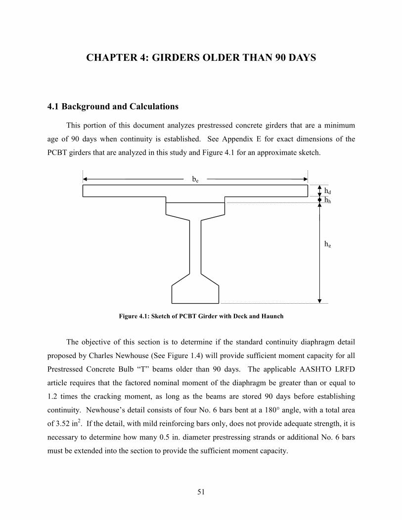
51
CHAPTER 4: GIRDERS OLDER THAN 90 DAYS
4.1 Background and Calculations
This portion of this document analyzes prestressed concrete girders that are a minimum
age of 90 days when continuity is established. See Appendix E for exact dimensions of the
PCBT girders that are analyzed in this study and Figure 4.1 for an approximate sketch.
Figure 4.1: Sketch of PCBT Girder with Deck and Haunch
The objective of this section is to determine if the standard continuity diaphragm detail
proposed by Charles Newhouse (See Figure 1.4) will provide sufficient moment capacity for all
Prestressed Concrete Bulb “T” beams older than 90 days. The applicable AASHTO LRFD
article requires that the factored nominal moment of the diaphragm be greater than or equal to
1.2 times the cracking moment, as long as the beams are stored 90 days before establishing
continuity. Newhouse’s detail consists of four No. 6 bars bent at a 180° angle, with a total area
of 3.52 in2. If the detail, with mild reinforcing bars only, does not provide adequate strength, it is
necessary to determine how many 0.5 in. diameter prestressing strands or additional No. 6 bars
must be extended into the section to provide the sufficient moment capacity.
be
hd hh
hg
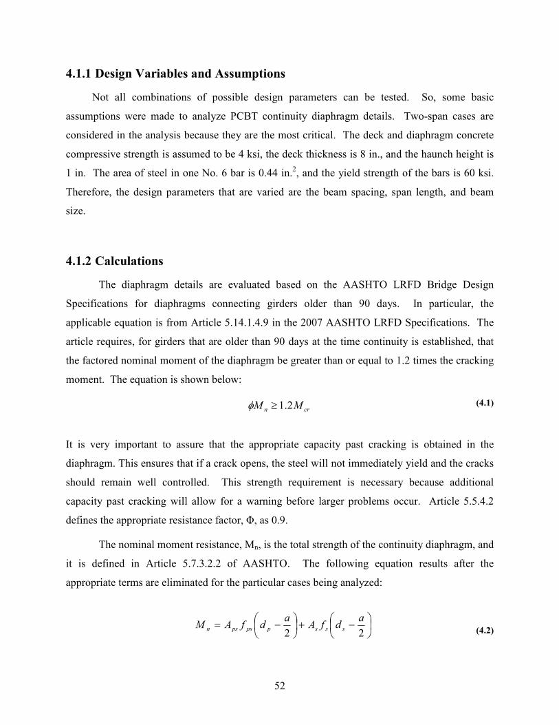
52
4.1.1 Design Variables and Assumptions
Not all combinations of possible design parameters can be tested. So, some basic
assumptions were made to analyze PCBT continuity diaphragm details. Two-span cases are
considered in the analysis because they are the most critical. The deck and diaphragm concrete
compressive strength is assumed to be 4 ksi, the deck thickness is 8 in., and the haunch height is
1 in. The area of steel in one No. 6 bar is 0.44 in.2, and the yield strength of the bars is 60 ksi.
Therefore, the design parameters that are varied are the beam spacing, span length, and beam
size.
4.1.2 Calculations
The diaphragm details are evaluated based on the AASHTO LRFD Bridge Design
Specifications for diaphragms connecting girders older than 90 days. In particular, the
applicable equation is from Article 5.14.1.4.9 in the 2007 AASHTO LRFD Specifications. The
article requires, for girders that are older than 90 days at the time continuity is established, that
the factored nominal moment of the diaphragm be greater than or equal to 1.2 times the cracking
moment. The equation is shown below:
(4.1)
It is very important to assure that the appropriate capacity past cracking is obtained in the
diaphragm. This ensures that if a crack opens, the steel will not immediately yield and the cracks
should remain well controlled. This strength requirement is necessary because additional
capacity past cracking will allow for a warning before larger problems occur. Article 5.5.4.2
defines the appropriate resistance factor, Φ, as 0.9.
The nominal moment resistance, Mn, is the total strength of the continuity diaphragm, and
it is defined in Article 5.7.3.2.2 of AASHTO. The following equation results after the
appropriate terms are eliminated for the particular cases being analyzed:
(4.2)
crn MM 2.1≥φ
−+
−=22
adfA
adfAM sssppspsn

53
where:
Aps = area of prestressing steel
fps = average stress in prestressing steel at nominal flexural resistance
dp = distance from extreme compression fiber to the centroid of prestressing tendons
a = depth of the compression block
As = area of non-prestressed tension reinforcement
fs = stress in the mild steel tension reinforcement at nominal flexural resistance
ds = distance from extreme compression fiber to the centroid of non-prestressed tensile
reinforcement
The area of prestressed and non-prestressed steel, the average stress in the mild steel, and the
distance from the extreme compression fiber of the member to the centroid of the prestressing
tendons and to the centroid of the non-prestressed steel can be easily determined. The area of
mild steel is based on the detail developed by Charles Newhouse, and is held constant. The area
of the prestressing steel is variable, so it is necessary to adjust the number of strands extended
into the continuity diaphragm until the factored nominal moment is greater than 1.2 times the
cracking moment for all of the cases that are tested.
Assuming that the strains are within the elastic range, the stress in one strand at general
slip can be taken as (Salmons 1975):
(4.3)
where:
Le = length of the strand
The strand length, Le, is calculated as the summation of “a” and “b” in the Figure 4.2.
According to the research done by the Missouri Department of Transportation and considering
the minimum lengths specified by AASHTO, the detail considered for this analysis has a value a
of 10 in. and a value b of 20 in. So, the total strand length is 30 in.
163.
25.8−= e
ps
Lf
54
Figure 4.2: Length of Prestressing Strand Extended into the Continuity Diaphragm
Due to the very broad top flange width (see Figure 4.1), the depth of the compression
block, a, can be assumed to be less than the depth of the deck. The equation to determine this
value is:
(4.4)
where:
beff = the effective flange width
f’c = the specified compression strength
Note that it is important to confirm that the depth of the compression block is indeed less than
the depth of the deck after it has been calculated.
The effective flange width, or beff, is defined in Article 4.6.2.6.1 of AASHTO, and must
be calculated to determine the depth of the compression block, a. So, beff is the least of:
• ¼ the effective span length
• 12 times the average depth of the deck, plus the greater of the web thickness or ½
the width of the top flange of the girder
• Average adjacent spacing of the girders
Concrete
Girder
b
Prestressing Strand
Continuity
Diaphragm
a
Deck
effc
pspsss
bf
fAfAa
'85.0
+=

55
Also, article 4.6.2.6 defines the effective span length for a continuous span as being “the distance
between the points of permanent load inflection”. So, for a two-span bridge, the distance
between points of permanent load inflection is half the span length.
The cracking moment must be found to determine if the diaphragm reinforcement is
adequate for girders older than 90 days. Article 5.7.3.3.2 of AASHTO defines the cracking
moment, Mcr, as being:
(4.5)
where:
fcpe = compressive stress in concrete due to effective prestress forces only (after allowance for
all prestress losses) at extreme fiber of section where tensile stress is caused by
externally applied loads
Mdnc = total unfactored dead load moment acting on the monolithic or noncomposite section
Sc = section modulus for the extreme fiber of the composite section when tensile stress is
caused by externally applied loads.
Snc = section modulus for the extreme fiber of the monolithic or noncomposite section where
tensile stress is caused by externally applied loads
fr = modulus of rupture
It is important to note that fcpe and Mdnc in the previous equation are equal to 0 for the purpose of
calculating the diaphragm cracking moment. Therefore, the above equation can be reduced to
(see Figure 4.1 for sketch of cross-section):
(4.6)
where:
Icomposite = the moment of inertia for the composite section
ycomposite = the distance from the bottom of the girder to the centroid of the composite section
Article 5.4.2.6 in the AASHTO LRFD Specifications defines the modulus of rupture, fr,
for normal weight concrete as:
rc
nc
cdnccperccr fS
S
SMffSM ≤
−−+= 1)(
r
composite
composite
rccr fy
IfSM ⋅==
56
(4.7)
Note that f’c, for the calculations in this section, refers to the compressive strength of the
diaphragm concrete, not the compressive strength of the girder.
4.1.3 Sample Calculations
Consider a PCBT-77 girder with a girder spacing of 8 ft and a span length of 130 ft. For
this study, the following parameters are considered to be constant:
• Diaphragm compressive strength of 4 ksi
• Slab thickness of 8 in.
• Haunch height of 1 in.
• Area of steel bars of 3.52 in.2 (Newhouse standard detail of four No. 6 bars bent
180°)
For this particular girder size, the following parameters can be found:
• Beam moment of inertia of 788,700 in.4
• Beam area of 970.7 in.2
• Beam height of 77 in.
• Distance from bottom of beam to centroid of 37.67 in.
See Appendix A for the calculations.
• 1.2 Mcr = 16,490 in.-k
• ΦMn = 16,930 in.-k
• No additional strands are needed
4.2 Results
As previously mentioned, it is important to determine how many prestressing strands or
additional mild reinforcing bars must be extended into diaphragms so that the total strength is
greater than 1.2 times the cracking moment for girders older than 90 days. A certain amount of
strength is obtained from the detail developed by Charles Newhouse, so the remaining strength
must come from the prestressing strands or the additional steel.
cr ff '24.0=
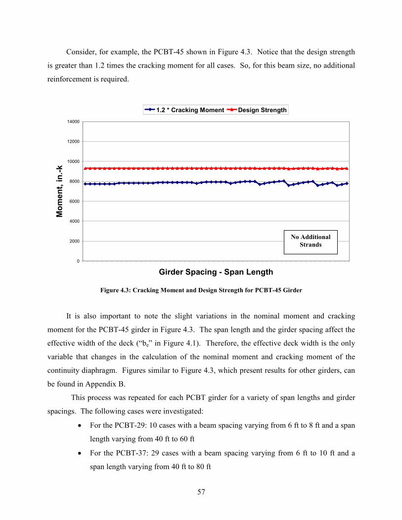
57
Consider, for example, the PCBT-45 shown in Figure 4.3. Notice that the design strength
is greater than 1.2 times the cracking moment for all cases. So, for this beam size, no additional
reinforcement is required.
0
2000
4000
6000
8000
10000
12000
14000
Girder Spacing - Span Length
Mo
me
nt,
in
.-k
1.2 * Cracking Moment Design Strength
Figure 4.3: Cracking Moment and Design Strength for PCBT-45 Girder
It is also important to note the slight variations in the nominal moment and cracking
moment for the PCBT-45 girder in Figure 4.3. The span length and the girder spacing affect the
effective width of the deck (“be” in Figure 4.1). Therefore, the effective deck width is the only
variable that changes in the calculation of the nominal moment and cracking moment of the
continuity diaphragm. Figures similar to Figure 4.3, which present results for other girders, can
be found in Appendix B.
This process was repeated for each PCBT girder for a variety of span lengths and girder
spacings. The following cases were investigated:
• For the PCBT-29: 10 cases with a beam spacing varying from 6 ft to 8 ft and a span
length varying from 40 ft to 60 ft
• For the PCBT-37: 29 cases with a beam spacing varying from 6 ft to 10 ft and a
span length varying from 40 ft to 80 ft
No Additional
Strands

58
• For the PCBT-45: 55 cases with a beam spacing varying from 6 ft to 10 ft and a
span length varying from 40 ft to 100 ft
• For the PCBT-53: 68 cases with a beam spacing varying from 6 ft to 10 ft and a
span length varying from 40 ft to 115 ft
• For the PCBT-61: 70 cases with a beam spacing varying from 6 ft to 10 ft and a
span length varying from 50 ft to 125 ft
• For the PCBT-69: 66 cases with a beam spacing varying from 6 ft to 10 ft and a
span length varying from 60 ft to 135 ft
• For the PCBT-77: 60 cases with a beam spacing varying from 6 ft to 10 ft and a
span length varying from 80 ft to 145 ft
• For the PCBT-85: 60 cases with a beam spacing varying from 6 ft to 10 ft and a
span length varying from 95 ft to 150 ft
• For the PCBT-93: 59 cases with a beam spacing varying from 6 ft to 10 ft and a
span length varying from 100 ft to 160 ft
4.3 Conclusions
For cases for which bars alone were not adequate, the numbers of strands were adjusted
until the design strength was at least 1.2 times the cracking moment for all cases. Table 4.1
presents the results.
Table 4.1: Bent Strands Required and Recommended for PCBT Girders
Girder # Bent Strands Required # Bent Strands Recommended
PCBT-29 0 0
PCBT-37 0 0
PCBT-45 0 0
PCBT-53 0 0
PCBT-61 0 0
PCBT-69 1 0
PCBT-77 1 2
PCBT-85 2 2
PCBT-93 2 2
59
Note that the PCBT-69 girder almost has sufficient moment capacity beyond the cracking
moment without any bent strands. In fact, the design strength was 1.17 times the cracking
moment, instead of the needed 1.2, for the worst case analyzed for this girder without bent
strands. Therefore, it is recommended that no additional strands be used because it is highly
likely that this detail is adequate without extended strands, but the decision to add strands should
be left to the discretion of the designer.
There is another option if extending prestressing strands into the diaphragm is not
preferable. If the designer would rather not extend prestressing strands, additional mild steel
could be used for the continuity diaphragm reinforcement. Using six, rather than four, No. 6 bars
bent at a 180° angle would provide adequate capacity for the diaphragm for all cases.
60
CHAPTER 5: GIRDERS YOUNGER THAN 90 DAYS
5.1 Introduction
Section 5.14.1.4.5 of the AASHTO LRFD Bridge Design Specifications gives two
conditions that can be used to determine if a bridge can be considered fully continuous for live
loads. Either a negative moment must develop over time in the diaphragm or the girders must be
at least 90 days old. It is important to determine when, if ever, the diaphragm moment will
become negative because it is not profitable to store girders longer than necessary. However,
one must be able to predict long-term effects in order to determine if the AASHTO requirement
is met for girders that are stored less than 90 days before continuity.
This chapter presents the method of calculating continuity diaphragm restraint moments
for girders younger than 90 days. The PCA Method was used in the analysis with the updated
creep and shrinkage models presented in the AASHTO LRFD Bridge Design Specifications.
The discussion of the models is followed by the presentation of calculations for time-dependent
effects in continuity diaphragms. Finally, an overview of the results and conclusions for PCBT
girders is presented towards the end of this chapter.
5.2 Models
Although time-dependent effects in prestressed concrete are fairly well understood, many
different models exist to calculate their influences. The two widely used models to determine
creep and shrinkage values for design today are the AASHTO LRFD Bridge Design
Specifications and the CEB-FIP Model Code 1990. This study was conducted to develop a
design aid for continuous concrete bridges with a cast-in-place deck for the Virginia Department
of Transportation (VDOT).
VDOT uses the AASHTO LRFD Specifications for design. Therefore, this study uses
the AASHTO creep, shrinkage, and prestress loss models with the PCA Method to determine the
time-dependent moments in the diaphragm, except Φ/(1+Φχ) is used instead of (1-e-Φ). These
two factors are generally equivalent, but Φ/(1+Φχ) is consistent with the prestress loss method.
To show that these two factors are equivalent, consider typical values of 2.0 for Φ and 0.7 for χ:

61
1-e-2 = 0.865
2/(1+0.7*2) = 0.833
Also, some additional consideration of the time-dependent moment that is applied to the
continuity diaphragm is in order. AASHTO states that the time-dependent moment must be
considered if it is positive because it produces a more critical result, but it should be ignored if it
is negative. This illustrates that there is much uncertainty in modeling the time-dependent
effects in concrete, so AASHTO chooses the conservative option of ignoring beneficial effects
but considering harmful ones.
The moments that must be calculated include the time-dependent, thermal, composite
dead load, and live load. This section presents the models used in the calculation of these
moments. A MathCAD spreadsheet was developed, using the AASHTO specifications, to
determine the restraint moment that will develop in the continuity diaphragm.
5.2.1 AASHTO Creep Model
According to AASHTO LRFD 2007 Bridge Design Specifications Section 5.4.2.3.2, the
creep coefficient can be calculated by using the following equations:
( 5.1)
(5.2)
(5.3)
(5.4)
(5.5)
where:
ψ(t,ti) = creep of a member at a given time, t, due to a load applied at an initial time, ti
H = relative humidity (%)
118.0
i 9.1)t(t,−= itdfhcvs tkkkkψ
0)/(13.045.1 ≥−= SVkvs
Hkhc 008.056.1 −=
ci
ff
k'1
5
+=
tf
tk
ci
td +−=
'461

62
kvs = factor for the effect of the volume-to-surface ratio of the component
kf = factor for the effect of the concrete strength
khc = humidity factor for creep
ktd = time development factor
t = maturity of concrete (days)
ti = age of concrete when the initial load is applied (days)
V/S = volume-to-surface area ratio (in.)
f’ci = specified compressive strength of concrete at time of prestressing (ksi)
Note that it can be observed that one day of accelerated steam curing is equal to 7 days of regular
curing. The above calculated factors can be used to predict the creep that will occur from any
time to any other time.
5.2.2 AASHTO Shrinkage Model
Section 5.4.2.3.3 of the AASHTO LRFD Interim 2005 Bridge Design Specifications
defines shrinkage as follows:
(5.6)
(5.7)
where:
εsh = shrinkage of a member
khs = humidity factor for shrinkage
All other factors correspond to those defined in section 5.1.1.
31048.0 −−= xkkkk tdfhsvsshε
Hkhs 014.000.2 −=
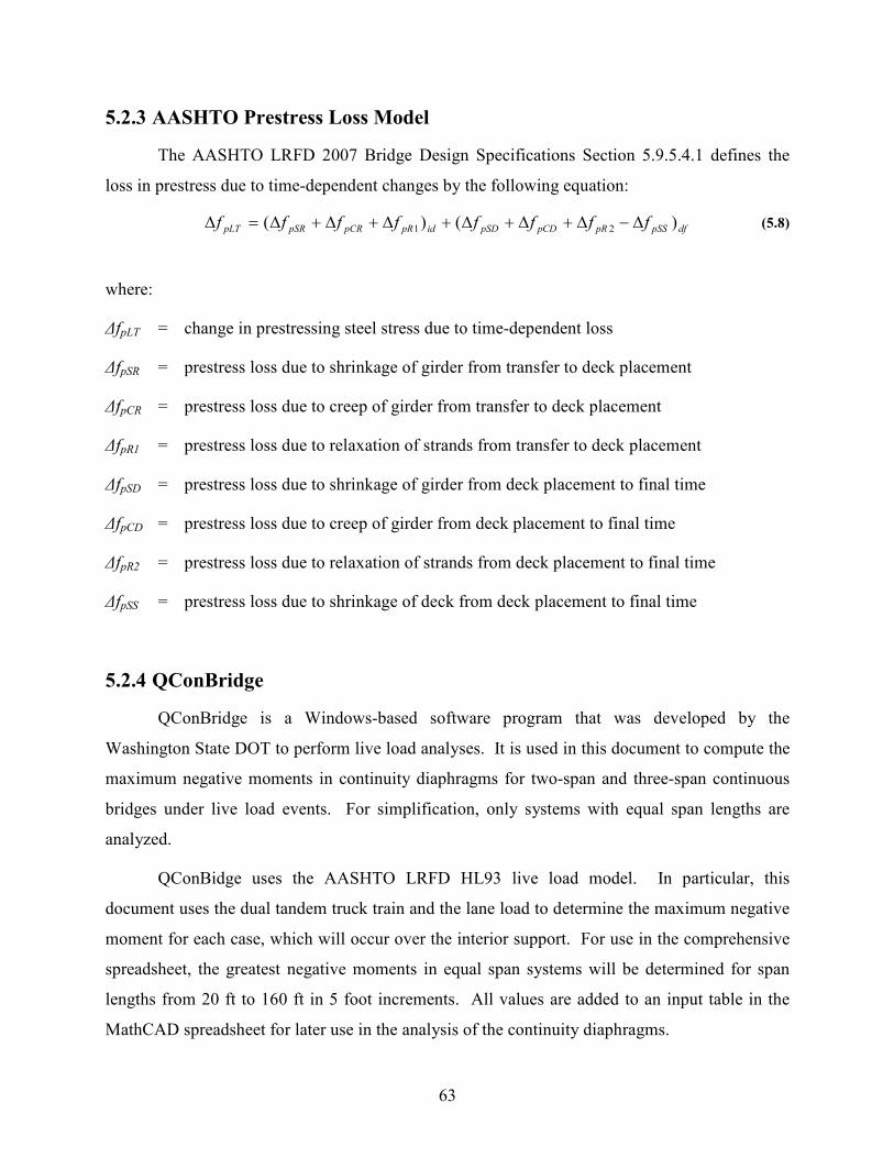
63
5.2.3 AASHTO Prestress Loss Model
The AASHTO LRFD 2007 Bridge Design Specifications Section 5.9.5.4.1 defines the
loss in prestress due to time-dependent changes by the following equation:
(5.8)
where:
∆fpLT = change in prestressing steel stress due to time-dependent loss
∆fpSR = prestress loss due to shrinkage of girder from transfer to deck placement
∆fpCR = prestress loss due to creep of girder from transfer to deck placement
∆fpR1 = prestress loss due to relaxation of strands from transfer to deck placement
∆fpSD = prestress loss due to shrinkage of girder from deck placement to final time
∆fpCD = prestress loss due to creep of girder from deck placement to final time
∆fpR2 = prestress loss due to relaxation of strands from deck placement to final time
∆fpSS = prestress loss due to shrinkage of deck from deck placement to final time
5.2.4 QConBridge
QConBridge is a Windows-based software program that was developed by the
Washington State DOT to perform live load analyses. It is used in this document to compute the
maximum negative moments in continuity diaphragms for two-span and three-span continuous
bridges under live load events. For simplification, only systems with equal span lengths are
analyzed.
QConBidge uses the AASHTO LRFD HL93 live load model. In particular, this
document uses the dual tandem truck train and the lane load to determine the maximum negative
moment for each case, which will occur over the interior support. For use in the comprehensive
spreadsheet, the greatest negative moments in equal span systems will be determined for span
lengths from 20 ft to 160 ft in 5 foot increments. All values are added to an input table in the
MathCAD spreadsheet for later use in the analysis of the continuity diaphragms.
dfpSSpRpCDpSDidpRpCRpSRpLT ffffffff )()( 21 ∆−∆+∆+∆+∆+∆+∆=∆

64
It is important to note that QConBridge calculates the maximum moments occurring in
the structure per lane loaded. However, analysis and design of bridges require that a critical
moment per beam be found. So, distribution factors are calculated and used to adjust the
moment per lane into a moment per beam. Spacing, deck thickness, and length requirements are
checked to make sure that AASHTO recommended distribution factors can be used.
5.2.5 Thermal Moment
As previously discussed, the thermal effects on a concrete bridge must be taken into
account (Imbsen, et al. 1985). The method suggested in the AASHTO LRFD Bridge Design
Specifications states that the equation to calculate the axial force in a fully restrained system due
to thermal effects is:
(5.9)
where:
E = elastic modulus
α = coefficient of thermal expansion
T(Y) = temperature at depth Y
b(Y) = net section width at height Y
σ(Y) = longitudinal stress at a fiber located a distance Y from the center of gravity of the cross-
section
P = restraining axial force
Likewise, the moment caused by the thermal forces in a fully restrained system is also defined in
NCHRP 276 and is as follows:
(5.10)
Figure 5.1 illustrates the AASHTO LRFD Zone 3 thermal gradient being applied to the PCBT
girder.
∫∫ ⋅=⋅⋅⋅=YY
dyYbYdyYbYTEP )()()()( σα
∫∫ ⋅⋅=⋅⋅⋅⋅=YY
YdyYbYYdyYbYTEM )()()()( σα

65
hf
hh
4 in.
2 in.
1.5 in.
S
47"
11"
P1P1
P2 P2
P3P3
P4P4
P5P5
41
11TA
TB
TC
TD
12"
4"
TE P6P6
7"
Figure 5.1: Thermal Forces in PCBT Girders
Note that the top and bottom sections of all PCBT girders are the same, so the difference
between girder sizes is in web heights. Therefore, the top part of the cross-section shown in
Figure 5.1 is valid for all PCBT girder sizes. The negative thermal gradient is not considered
because it causes beneficial negative moments over interior supports. See the design example in
Appendix C for sample calculations of forces P1 through P6 and for temperatures TA through
TE.
Also, notice assumptions made in the model regarding the thickness of the deck and the
haunch. Figure 5.1 is based on the assumption that the thickness of the deck is at least 4 in., so
the temperature of 11°F is acting in the deck. This is a valid assumption because the VDOT
standard specification design aid states that the thickness of the deck should range between 7.5
in. and 8.5 in. (VDOT 2005). In addition, the depth of the deck and haunch together must be at
least 8.5 in., so that the temperature gradient reaches 0°F at or before the point labeled “TE” in
Figure 5.1. This is a valid assumption because the height of the haunch can be assumed to be at
least 1 in. in all cases.
It is important to note that the restraint moment at the interior support is 1.5 times the
moment that acts on the end of a beam. See Figure 5.2.

66
Figure 5.2: Restraint Moment
5.3 Calculations
The PCA Method was used with the improved creep, shrinkage, and prestress loss
models, discussed in the previous section, to analyze the time-dependent moments in PCBT
girder diaphragms.
5.3.1 Cases Analyzed
For each PCBT girder size, the following cases were analyzed:
• 6 ksi compressive strength, average span length, and narrowest girder spacing
• 6 ksi compressive strength, long span length, and narrowest girder spacing
• 8 ksi compressive strength, average span length, and narrowest girder spacing
• 8 ksi compressive strength, long span length, and narrowest girder spacing
• 6 ksi compressive strength, average span length, and widest girder spacing
• 6 ksi compressive strength, long span length, and widest girder spacing
• 8 ksi compressive strength, average span length, and widest girder spacing
• 8 ksi compressive strength, long span length, and widest girder spacing
These cases were selected because they are considered to be the extreme cases, so they provide
bounds for the typical design parameters. The “long span length” was the greatest span length
according to the VDOT design aid for a particular girder with a specified compressive strength
and girder spacing, and the “average span length” was considered to be about 20 to 25 ft shorter
P M
P M
.5 M
M 1.5 M
67
than the greatest span length. Likewise, the “narrowest girder spacing” was considered to be the
smallest girder spacing available on the VDOT design aid for a particular girder size, girder
spacing, and compressive strength, while the “widest girder spacing” was the largest girder
spacing available.
5.3.2 MathCAD Spreadsheet
The following is a brief description of the calculations that are performed in the
MathCAD spreadsheet in Appendix C:
• Input:
o Beam and deck properties
o Span length
o Strand pattern (including number of strands harped)
o Live loads from QConBridge
• Intermediate Calculations:
o Calculate transformed cross-sectional properties
o Check allowable stresses at transfer
o Calculate creep and shrinkage coefficients
� From initial time to deck placement
� From deck placement to end of service
o Calculate prestress loss
� From initial time to deck placement
� From deck placement to end of service
o Check stresses at deck placement
o Calculate composite cross-sectional properties
o Calculate cracking moment of diaphragm

68
• Time-dependent Calculations:
o Calculate dead load creep rotation
o Find the moment to restrain the dead load creep rotation
o Calculate the end rotation due to prestress
o Find the moment to restrain prestress rotations
o Subtract effects of rotation from transfer to deck placement and calculate
reduced restraint moment
o Calculate the diaphragm restraint moment due to loss of prestress
o Calculate differential shrinkage restraint moment
o Find the total time-dependent moment in the diaphragm
• Final Calculations:
o Check stresses at end of service
o Calculate the thermal restraint moment
o Calculate the nominal moment capacity of the diaphragm
o Check if the AASHTO requirements are satisfied
o Check the flexural strength of the diaphragm
5.4 Results
A comprehensive MathCAD spreadsheet was developed to perform all calculations. See
Appendix C for the comprehensive spreadsheet of a two span system. The three-span system is
shown in Appendix D. The highlighted fields in the Appendices represent input values that can
be adjusted to represent any situation. Results from runs of the MathCAD sheet were recorded
in an EXCEL spreadsheet for further analysis. The objective was to determine how many days
each PCBT girder must be stored so that positive time-dependent moments will not develop in
the continuity diaphragm.

69
5.4.1 Interpreting Results
Figure 5.3 is a plot of the individual components of the restraint moment in the
diaphragm for an average analysis case. These components include the time-dependent, dead
load on composite, live load, and thermal restraint moments. The example presented in Figure
5.3 is a PCBT-61 girder with 8 ksi compressive strength concrete, a wide girder spacing (10 ft),
and an average span length (60 ft) for the given girder size. As specified by AASHTO, the
modified total does not include the contribution of the time-dependent restraint moment if it is
negative, but does include it if it is positive. Figure 5.3 illustrates how the restraint moments will
change depending on the number of days the girders are stored before they are made continuous
and composite. For other cases that were analyzed in this study, the magnitudes of the values in
Figure 5.3 are different, but the general patterns are similar.
-1800.0
-1500.0
-1200.0
-900.0
-600.0
-300.0
0.0
300.0
600.0
900.0
1200.0
1500.0
0 10 20 30 40 50 60 70 80 90
Girder Age at Continuity (days)
Dia
ph
rag
m R
es
tra
int
Mo
me
nt
(k-f
t)
Time Dependant
Dead Load
1/2 Live Load
Thermal
Total
Modified Total
Figure 5.3: Continuity Diaphragm Restraint Moments
Note the magnitude of the positive thermal restraint moment compared to the dead load
and live load restraint moment. The positive thermal moment is greater than the sum of the
composite dead load and half of the life load. Also notice that that the modified total moment,
which does not include the contribution of the time-dependent moment when it is negative, never
is negative for this example. This means that this additional criterion involving the modified
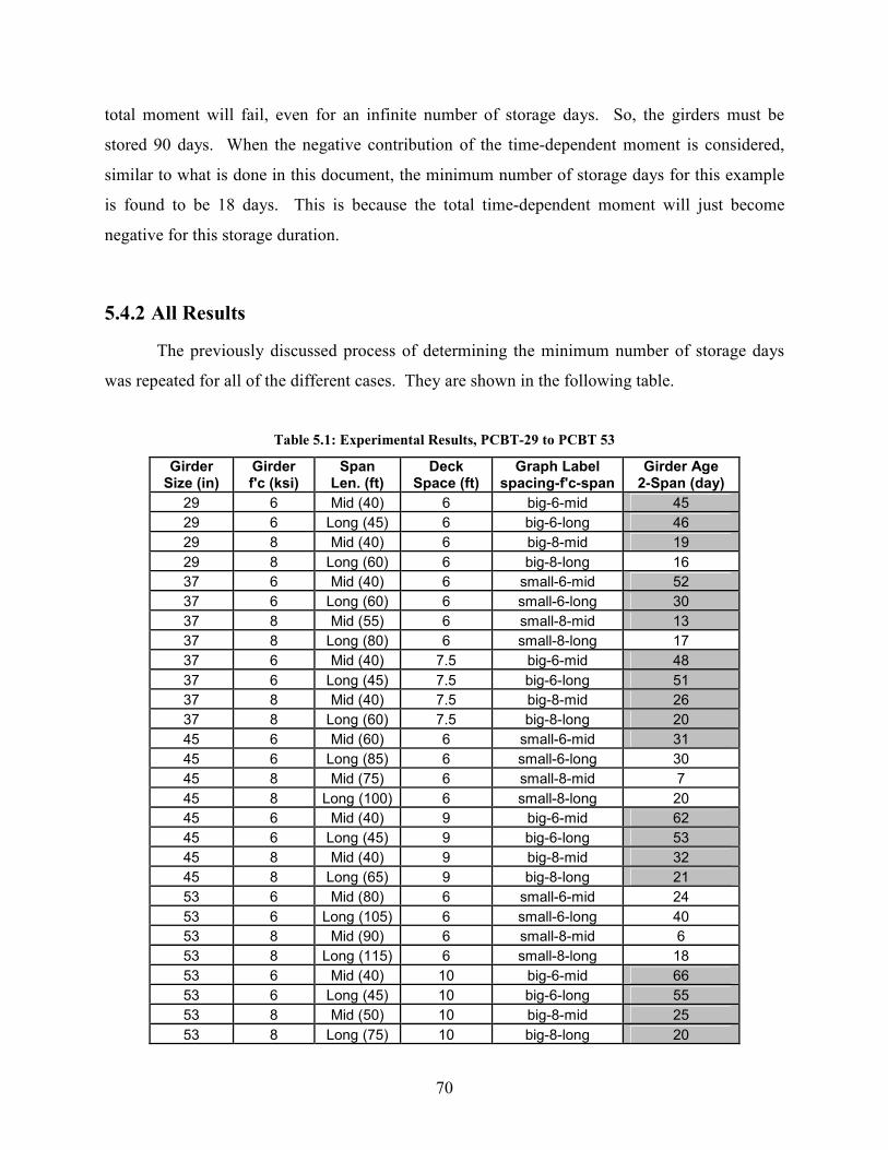
70
total moment will fail, even for an infinite number of storage days. So, the girders must be
stored 90 days. When the negative contribution of the time-dependent moment is considered,
similar to what is done in this document, the minimum number of storage days for this example
is found to be 18 days. This is because the total time-dependent moment will just become
negative for this storage duration.
5.4.2 All Results
The previously discussed process of determining the minimum number of storage days
was repeated for all of the different cases. They are shown in the following table.
Table 5.1: Experimental Results, PCBT-29 to PCBT 53
Girder Size (in)
Girder f'c (ksi)
Span Len. (ft)
Deck Space (ft)
Graph Label spacing-f'c-span
Girder Age 2-Span (day)
29 6 Mid (40) 6 big-6-mid 45
29 6 Long (45) 6 big-6-long 46
29 8 Mid (40) 6 big-8-mid 19
29 8 Long (60) 6 big-8-long 16
37 6 Mid (40) 6 small-6-mid 52
37 6 Long (60) 6 small-6-long 30
37 8 Mid (55) 6 small-8-mid 13
37 8 Long (80) 6 small-8-long 17
37 6 Mid (40) 7.5 big-6-mid 48
37 6 Long (45) 7.5 big-6-long 51
37 8 Mid (40) 7.5 big-8-mid 26
37 8 Long (60) 7.5 big-8-long 20
45 6 Mid (60) 6 small-6-mid 31
45 6 Long (85) 6 small-6-long 30
45 8 Mid (75) 6 small-8-mid 7
45 8 Long (100) 6 small-8-long 20
45 6 Mid (40) 9 big-6-mid 62
45 6 Long (45) 9 big-6-long 53
45 8 Mid (40) 9 big-8-mid 32
45 8 Long (65) 9 big-8-long 21
53 6 Mid (80) 6 small-6-mid 24
53 6 Long (105) 6 small-6-long 40
53 8 Mid (90) 6 small-8-mid 6
53 8 Long (115) 6 small-8-long 18
53 6 Mid (40) 10 big-6-mid 66
53 6 Long (45) 10 big-6-long 55
53 8 Mid (50) 10 big-8-mid 25
53 8 Long (75) 10 big-8-long 20
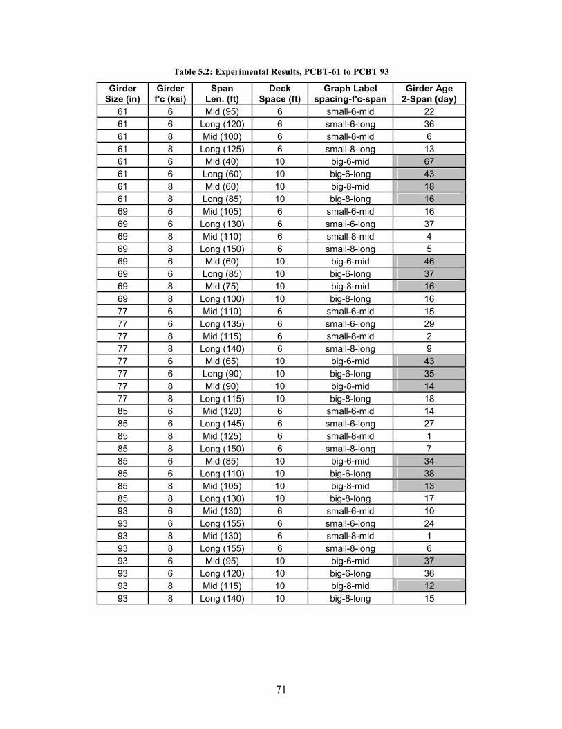
71
Table 5.2: Experimental Results, PCBT-61 to PCBT 93
Girder Size (in)
Girder f'c (ksi)
Span Len. (ft)
Deck Space (ft)
Graph Label spacing-f'c-span
Girder Age 2-Span (day)
61 6 Mid (95) 6 small-6-mid 22
61 6 Long (120) 6 small-6-long 36
61 8 Mid (100) 6 small-8-mid 6
61 8 Long (125) 6 small-8-long 13
61 6 Mid (40) 10 big-6-mid 67
61 6 Long (60) 10 big-6-long 43
61 8 Mid (60) 10 big-8-mid 18
61 8 Long (85) 10 big-8-long 16
69 6 Mid (105) 6 small-6-mid 16
69 6 Long (130) 6 small-6-long 37
69 8 Mid (110) 6 small-8-mid 4
69 8 Long (150) 6 small-8-long 5
69 6 Mid (60) 10 big-6-mid 46
69 6 Long (85) 10 big-6-long 37
69 8 Mid (75) 10 big-8-mid 16
69 8 Long (100) 10 big-8-long 16
77 6 Mid (110) 6 small-6-mid 15
77 6 Long (135) 6 small-6-long 29
77 8 Mid (115) 6 small-8-mid 2
77 8 Long (140) 6 small-8-long 9
77 6 Mid (65) 10 big-6-mid 43
77 6 Long (90) 10 big-6-long 35
77 8 Mid (90) 10 big-8-mid 14
77 8 Long (115) 10 big-8-long 18
85 6 Mid (120) 6 small-6-mid 14
85 6 Long (145) 6 small-6-long 27
85 8 Mid (125) 6 small-8-mid 1
85 8 Long (150) 6 small-8-long 7
85 6 Mid (85) 10 big-6-mid 34
85 6 Long (110) 10 big-6-long 38
85 8 Mid (105) 10 big-8-mid 13
85 8 Long (130) 10 big-8-long 17
93 6 Mid (130) 6 small-6-mid 10
93 6 Long (155) 6 small-6-long 24
93 8 Mid (130) 6 small-8-mid 1
93 8 Long (155) 6 small-8-long 6
93 6 Mid (95) 10 big-6-mid 37
93 6 Long (120) 10 big-6-long 36
93 8 Mid (115) 10 big-8-mid 12
93 8 Long (140) 10 big-8-long 15
72
The highlighted cases in Table 5.1 and Table 5.2 are those that failed the AASHTO requirement,
which excludes the contribution of the time-dependent moment if it negative. Therefore, the
highlighted cases would need to be stored 90 days since the total moment in the diaphragm will
never be negative (because then effects due to negative time-dependent moments must be
ignored). There are many of these cases.
5.4.3 General Trends
There are general trends among the results. It is important to recognize and understand
these patterns so that continuity diaphragm restraint moments can be better understood.
5.4.3.1 Changes in Length
No comprehensive conclusions can be drawn to compare the change that occurs in the total
restraint moment due to changes in the length of the member. In some cases, moving from an
average span length to a long span length required a longer storage period for the girders, and in
others a shorter storage period resulted. It is difficult to directly determine the effects of
adjusting the span length on the total diaphragm restraint moment, because the span length
affects all of the individual components of the total restraint moment in different ways.
However, the following observations can be noted as span lengths increase for a given number of
storage days:
• The thermal moment will not change
• The live load moment will become more negative
• The dead load moment will become more negative
• The time-dependent moment could become either more positive or negative depending
on the magnitudes of the changes in the following components:
o The moment to restrain the dead load creep rotation will become more negative
o The moment to restrain prestress creep rotations will become more positive
o The moment to restrain the creep of prestress losses will become more positive
o The differential shrinkage restraint moment will not change

73
5.4.3.2 Changes in Compressive Strength
Analysis of the results showed that there was a decrease in the minimum number of
storage days when the girder compressive strength was increased from 6 ksi to 8 ksi. The
average decrease in the minimum storage days was 65.5%. The largest reduction occurred in the
cases consisting of the medium span lengths with the closer girder spacing, which was an
average decrease of 80.6% for the cases tested. The smallest reduction occurred in the cases
consisting of the long span lengths with the wide girder spacing, which was a decrease of 59.2%.
The decrease in the minimum number of storage days for girders as compressive strength
increases is due to several factors. First of all, as the compressive strength increases, there are
changes in the transformed area and in the centroid of the transformed area. This will have
numerous effects on the calculation of total restraint moment. Also, the ultimate creep and
shrinkage will decrease as the concrete strength increases. Therefore, there is a decrease in the
minimum number of days that a girder needs to be stored so that the remaining time-dependent
effects will not cause positive moments in the diaphragm.
5.4.3.3 Changes in Girder Spacing
The results of the analyzed cases show that there was a 137% average increase in the
number of days that the girders needed to be stored so that a positive moment would not develop
in the diaphragm when the girder spacing increases from the close to the wide spacing. A larger
compressive strength results in a greater degree of change when the girder spacing is adjusted.
Also, a more average span length results in greater changes as well. Hence, there is only a
moderate (24%) increase in the minimum number of storage days when the girder spacing is
changed from close to wide for the cases consisting of the 6 ksi compressive strength with the
long span lengths
The girder spacing has several effects on the continuity diaphragm restraint moments.
First of all, the dead load moment of the structure in the continuity diaphragm will become more
negative as the deck width increases. Likewise, the live load moment in the continuity
diaphragm will also become more negative as the deck width increases because the girder
distribution factors will increase. Also, differential shrinkage between the deck and the girders
74
increases because a larger volume of the deck results in a greater shrinkage force in the deck.
Most importantly, the thermal gradient that was used in this analysis has a very large component
that is applied to the top of the deck. So, increasing the width of the deck substantially increases
the positive thermal restraint moment in the continuity diaphragm that needs to be counteracted
by the other moments.
5.4.4 Two-Spans vs. Three-Spans
Although it was previously assumed that two-span cases are critical, three-span systems
must be further explored because time-dependent factors are interdependent. Appendix D shows
a comparison of the calculated terms that change between the two-span and three-span systems.
When moving from a two-span case to a three-span case, the composite dead load restraint
moment becomes less negative, the live load restraint moment becomes less negative, the
thermal restraint moment becomes less positive, the non-composite dead load restraint moment
becomes less negative, the prestress restraint moment becomes less positive, and the differential
shrinkage moment becomes less negative. Several tests were run on about half of the PCBT
girders to compare the two-span and the three span-cases. The results are shown in Table 5.3
The two-span systems are critical for all cases, as shown in Table 5.3. This means that
the PCBT girders need to be stored for fewer days before establishing continuity so that a
negative diaphragm moment will result. Therefore, it is a valid assumption that the two-span
cases are critical and are the only ones that need to be computed.

75
Table 5.3: Three-Span Systems vs. Two-Span Systems: Minimum Storage Duration
Girder Size (in)
Girder f'c (ksi)
Span Len. (ft)
Deck Space (ft)
Graph Label space-f'c-span
Girder Age 2-Span (day)
Girder Age 3-Span (day)
29 6 Mid (40) 6 big-6-mid 45 39
29 6 Long (45) 6 big-6-long 46 40
29 8 Mid (40) 6 big-8-mid 19 16
29 8 Long (60) 6 big-8-long 16 14
45 6 Mid (60) 6 small-6-mid 31 28
45 6 Long (85) 6 small-6-long 30 23
45 8 Mid (75) 6 small-8-mid 7 6
45 8 Long (100) 6 small-8-long 20 12
45 6 Mid (40) 9 big-6-mid 62 55
45 6 Long (45) 9 big-6-long 53 47
45 8 Mid (40) 9 big-8-mid 32 29
45 8 Long (65) 9 big-8-long 21 19
61 6 Mid (95) 6 small-6-mid 22 19
61 6 Long (120) 6 small-6-long 36 23
61 8 Mid (100) 6 small-8-mid 6 4
61 8 Long (125) 6 small-8-long 13 7
61 6 Mid (40) 10 big-6-mid 67 61
61 6 Long (60) 10 big-6-long 43 39
61 8 Mid (60) 10 big-8-mid 18 16
61 8 Long (85) 10 big-8-long 16 4
77 6 Mid (110) 6 small-6-mid 15 12
77 6 Long (135) 6 small-6-long 29 20
77 8 Mid (115) 6 small-8-mid 2 1
77 8 Long (140) 6 small-8-long 9 7
77 6 Mid (65) 10 big-6-mid 43 39
77 6 Long (90) 10 big-6-long 35 31
77 8 Mid (90) 10 big-8-mid 14 12
77 8 Long (115) 10 big-8-long 18 18
93 6 Mid (130) 6 small-6-mid 10 7
93 6 Long (155) 6 small-6-long 24 16
93 8 Mid (130) 6 small-8-mid 1 1
93 8 Long (155) 6 small-8-long 6 4
93 6 Mid (95) 10 big-6-mid 37 33
93 6 Long (120) 10 big-6-long 36 32
93 8 Mid (115) 10 big-8-mid 12 10
93 8 Long (140) 10 big-8-long 15 13
5.5 Conclusions
If the designer is willing to perform a somewhat involved analysis, the number of girder
storage days can be reduced significantly below 90 days about half of the time. For the other
half of the cases that must be stored for 90 days, the total moment in the diaphragm will never
76
become negative because the contributions of the negative time-dependent moment must be
ignored.
If the negative time-dependent restraint moments are considered, the largest minimum
number of storage days for girders with a compressive strength of 6 ksi is 67 days and the largest
minimum number of storage days for girders with a compressive strength of 8 ksi is 32 days.
Note that including the negative time-dependent restraint moments in analysis of girders with a
compressive strength of 8 ksi cause a substantial reduction (32 days from 90 days) in the greatest
minimum storage duration. In general, narrower girder spacing and higher concrete compressive
strength results in shorter required storage duration.
A quick check can be done to see if girders must be stored 90 days. If the sum of the
thermal, composite dead load, and half of the live load restraint moments is positive, then the
girder must be stored 90 days. This is true because the only restraint moment that varies over
time is the time-dependent moment, which must be ignored if it is negative. If the sum of the
thermal, composite dead load, and half of the live load restraint moments is negative, then it is
very likely that the girder will be able to be stored for less than 90 days. In this case, it would be
beneficial to calculate the time-dependent restraint moment and determine the minimum number
of storage days that would result in a negative diaphragm restraint moment.
77
CHAPTER 6: CONCLUSIONS AND RECOMMENDATIONS
6.1 Conclusions and Recommendations
Several conclusions can be drawn from the research presented in this document that will
assist in the design of continuity diaphragms for PCBT girders. The topics that are discussed
include Testing the PCA Method, Girders Younger than 90 days, and Girders Older than 90
days.
6.1.1 Testing the PCA Method
The stresses throughout the cross-section of a composite bridge system were computed
using the PCA Method and then were compared to those found using the Separate Sections
Method (or the Trost-Menn Method) to determine accuracy. The PCA Method generally
produced conservative estimates of all stresses, and the girder creep coefficient is always a
conservative estimation of the creep coefficient that would give results similar to those obtained
using the Separate Sections Method. Also, this method is fairly accurate when the girder and the
deck creep coefficients are the same, or similar. However, more error is introduced as the creep
coefficients become more different from each other, but the method is still overall conservative.
Therefore, it has been concluded that the PCA Method adequately predicts the restraint moments
that develop in continuity diaphragms due to time-dependent effects.
6.1.2 Girders Older than 90 Days
This section determined how many bent strands need to be extended into continuity
diaphragms, in addition to Charles Newhouse’s standard detail (see Figure 1.4), to provide
sufficient moment capacity for PCBT girders. The applicable AASHTO LRFD article requires,
for girders that are older than 90 days at the time continuity is established, that the factored
nominal moment of the diaphragm be greater than or equal to 1.2 times the cracking moment.
Several girder spacings and span lengths were considered for each girder size.
78
It was concluded that no additional strands are required for the PCBT-29, PCBT-37,
PCBT-45, PCBT-53, and PCBT-61. For the PCBT-69, the design strength was 1.17 times the
cracking moment for the worst case analyzed without bent strands, instead of the required 1.2.
Therefore, it is highly likely that this detail is adequate without extended strands, but the decision
to add strands should be left to the discretion of the designer. The PCBT-77, PCBT-85, and the
PCBT-93 require one or two additional bent strands. So, it is recommended that two bent strands
be extended into the continuity diaphragm for these three girder sizes.
6.1.3 Girders Younger than 90 Days
The AASHTO LRFD Bridge Design Specifications were used to analyze PCBT girders
that are younger than 90 days when continuity is established. AASHTO states that a negative
moment must develop in the diaphragm if the girder is stored for less than 90 days before being
erected. In addition, the time-dependent moment must be considered if it is positive because it
produces a more critical result, but it should be ignored if it is negative. The goal of this aspect
of the research was to determine the minimum number of days that PCBT girders need to be
stored so that the AASHTO specifications are met.
It was found that if negative time-dependent moments are considered, 67 days is the
longest that a PCBT girder needs to be stored for the cases analyzed. However, half of the cases
must be stored for 90 days if the negative time-dependent effects are ignored. The factors that
seemed to contribute to the necessary 90 day storage time were average span lengths, wide girder
spacings, and lower compressive strengths.
If negative time-dependent moments are considered, there are general trends in the data.
Analysis of the results showed that there was a decrease in the minimum number of storage days
when the girder compressive strength was increased from 6 ksi to 8 ksi and when the girder
spacing decreased from the widest spacing to the closest spacing. However, no comprehensive
conclusions could be drawn to compare the change that occurs in the total restraint moment due
to changes in the length of the member.
Three-span systems were also considered, but the two-span systems were found to be
critical for all of the cases in this study. In other words, the PCBT girders need to be stored for
fewer days before establishing continuity (so that a negative diaphragm moment will result) if
79
they are used in three-span systems rather than two-span systems. This is true if negative time-
dependent moments are considered or if they are ignored.
6.2 Recommendations for Future Work
The results of this research produce additional questions. First of all, is there a more
accurate creep coefficient that can be used in place of the girder creep coefficient when
determining stresses in composite systems using the PCA Method? This study showed that
although the PCA Method was almost always conservative, the girder creep coefficient was not
always close to being accurate. This is especially true if the girder and deck coefficient were not
similar. More work is needed to determine if the girder creep coefficient can be simply adjusted
for use in the PCA Method to give more accurate results. Also, additional aging coefficients
should be considered. This study only considers an aging coefficient of 0.8, which could have a
significant impact on the appropriate creep coefficient that should be used in the PCA Method.
Secondly, the behavior of creep and shrinkage are fairly well understood, but there are
many different ways to model this behavior. This has been complicated by the many recent
advances in the material properties of concrete, which could require older methods of analysis to
be further updated. For example, thirty years ago the compressive strength of a typical concrete
bridge girder was somewhere between 3000 to 6000 psi, and models existed that calculated the
associated time-dependent effects fairly accurately. Since then, a greater understanding of the
properties and performance of concrete has been achieved. Concrete mixes now include
components, admixtures, and mix proportions considerably different from those in the past. The
result is more durable concrete that typically has a compressive strength anywhere from 4000 psi
to 10,000 psi. So, it stands to reason that new models should be developed to analyze and design
more modern concrete.
In particular, more research is needed to improve the models that analyze prestressed
concrete bridge girders made composite with a cast-in-place concrete deck and made continuous
over two or more spans. The AASHTO LRFD Bridge Design Specification asserts that the
restraint moments that develop in the continuity diaphragm are a function of many factors
including time-dependent effects, superimposed permanent load, settlement, live load, and a
temperature gradient. The effects that these factors have on restraint moments are still being
80
explored. Also, additional factors that could possibly contribute to the restraint moments are
being considered.
Also, additional design parameters could be varied for PCBT girders that are stored for
more than 90 days before erection. For the girders in this study, only the girders’ spacings and
span lengths were varied for each size girder. So, the diaphragm compressive strength, slab
thickness, and haunch height were held constant. The results presented in this study make use of
typical design parameters used by VDOT, but varying these parameters could provide more
comprehensive results for all possible cases.
Additionally, further research regarding the thermal restraint moment would be
beneficial. Although a standard thermal gradient exists for Virginia, experimental testing could
improve upon the existing design values. This research illustrated that the thermal restraint
moment calculated using the AASHTO thermal gradient was dominant in the design of
continuity diaphragm. Therefore, VDOT should consider evaluating a thermal gradient
specifically for Virginia to assure that the AASHTO gradient is appropriate. Installing
thermocouples into new bridge systems would allow researchers to see how temperature changes
through the life of the concrete due to environmental factors. Also, attaching strain gauges to a
concrete girder that is part of a bridge would provide insight as to how temperature affects strain
due to the surrounding temperatures.
Finally, additional design parameters could also be varied for PCBT girders that are less
than 90 days old before they are made composite and continuous. Only different values for the
span lengths, girder spacings, and girder compressive strengths were considered for the PCBT
girders younger than 90 days. Other design parameters that could be varied to provide a more
comprehensive understanding of the results include the age of girder at transfer of prestressing,
haunch height, and deck concrete compressive strength. In addition, a sensitivity analysis could
be performed on the aging coefficient to determine the magnitude of change that would result
from adjusting this parameter.
81
REFERENCES
American Association of State Highway and Transportation Officials (AASHTO), (2004).
AASHTO LRFD Bridge Design Specifications - Third Edition with 2005 and 2006 Interims.
Washington, D.C.
American Concrete Institute (ACI) Manual of Concrete Practice (2002). “Prediction of Creep,
Shrinkage, and Temperature Effects in Concrete Structures.” ACI 209R-92. Farmington Hills,
Michigan.
American Concrete Institute (ACI) Manual of Concrete Practice (2002). “Report on Factors
Affecting Shrinkage and Creep of Hardened Concrete.” ACI 209R-05. Farmington Hills,
Michigan.
Bazant, Z.P. (1975). “Theory of Creep and Shrinkage in Concrete Structures: A precis of recent
developments." Mechanics Today. American Academy of Mechanics, Vol. 2. Pergamon, New
York.
British Standards Institution, “Steel, Concrete and Composite Bridge, Part I, General Statement.”
British Standard BS 5400. Crowthorne, Berkshire, England (1978).
Dimmerling, A., Miller, R. A., Reid, C., Mirmiran, A., Hastak, M., and Baseheart, T. M. (2005).
“Connections Between Simply Supported Concrete Beams Made Continuous – Results of
NCHRP Project 12-53.” Transportation Research Record: Journal of the Transportation
Research Board, No. 1928. Transportation Research Board of the National Academies,
Washington, D.C.
Freyermuth, C. L. (1969). “Design of Continuous Highway Bridges with Precast, Prestressed
Concrete Girders.” Journal of the Prestressed Concrete Institute, Vol. 14, No 2.
Hognestad, E., Mattock, A. H., Karr, P. H. (1960). “Composite Construction for Continuity.”
Journal of the Prestressed Concrete Institute, Vol. 5, No 1.
Imbsen, A., Vandershaf, D.E., Schamber, R. A., and Nutt, R.V. (1985). “Thermal Effects in
Concrete Bridge Superstructures.” National Cooperative Highway Research Program Report
276, National Research Council, Washington, D.C.
MacGregor, J. G., and Wright, J. K. (2005). Reinforced Concrete: Mechanics and Design 4th
Edition. Pearson Prentice Hall, Upper Saddle River, New Jersey.
Mattock, A. H. (1961). “Precast-Prestress Concrete Bridges: 5. Creep and Shrinkage Studies.
Development Department Bulletin D46.” Portland Cement Association, Research and
Development Laboratories, Vol. 3, No 2. Stokie, Illinois.
82
Mattock, A. H., Kaar, P. H. (1960). “Continuous Precast-Prestressed Concrete Bridges.
Development Department Bulletin D43.” Portland Cement Association, Research and
Development Laboratories, Vol. 2, No. 5. Stokie, Illinois.
Menn, C. (1986). Prestressed Concrete Bridges, translated by Gauvreau, P., originally published
as Stahlbentonbruken, Springer-Berlag, Wein. Vienna, Austria.
Newhouse, C. D. (2005). “Design and Behavior of Prestressed, Precast Girders Made
Continuous – An Analytical and Experimental Study.” Ph.D. Dissertation, Virginia Tech.
Nilson, A. H. (1987), Design of Prestressed Concrete – Second Edition, John Wiley and Sons.
New York, NY.
Oesterle, R.G., Glikin, J.D., and Larson, S.C. (1989). “Design of Precast Prestressed Girders
Made Continuous.” National Cooperative Highway Research Program Report 322, National
Research Council, Washington, D.C.
Potgieter, I.C., and Gamble, W.L. (1983). “Response of Highway Bridges to Nonlinear
Temperature Distributions.” Rep. No. FHWA/IL/UI-201, University of Illinois at Urbana-
Champaign, Urbana-Champaign, IL.
Salmons, J.R. (1974). “End Connections of Pretensioned I-Beam Bridges”, Missouri
Cooperative Highway Report 73-5C. Missouri State Highway Department, Jefferson City,
Missouri.
Virginia Department of Transportation (2006). “Volume V – Part 2: Design Aids – Typical
Details.” <http://www.vdot.virginia.gov/business/bridge-v5p2.asp>
Washington State Department of Transportation (2005). Bridge Engineering Software-
QConBridges
<http://www.wsdot.wa.gov/eesc/bridge/software/index.cfm?fuseaction=software_detail&softwar
e_id=48>

beff 96 in=
beff min b( ):=
b
.125 l⋅
12 hd⋅ 7in+
s
:=
Effective width:
Astrand .153in2
:=
strands 1:=
yb 37.67in:=
hb 77in:=
Ab 970.7in2
:=
Ib 788700in4
:=
As 3.52in2
:=
hh 1in:=
hd 8in:=
fc 4ksi:=
l 130ft:=
s 8ft:=
Variables (PCBT Girder):
klfk
ft:=
ksik
in2
:=psi
lb
in2
:=
kin k in⋅:=µε .000001:=
kft k ft⋅:=
pcflb
ft3
:=k 1000lb:=Unit definition:
These calculations: PCBT-77 with a beam spacing of 8 ft and a span length of 130 ft
APPENDIX A: Design of Continuity Diaphragms for Girders Older than 90 Days
83
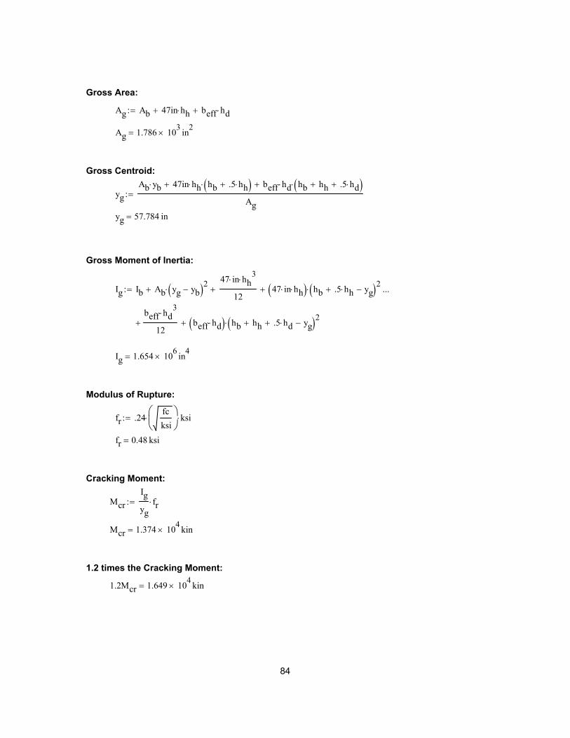
1.2Mcr 1.649 104
× kin=
1.2 times the Cracking Moment:
Mcr 1.374 104
× kin=
Mcr
Ig
yg
fr⋅:=
Cracking Moment:
fr 0.48 ksi=
fr .24fc
ksi
⋅ ksi⋅:=
Modulus of Rupture:
Ig 1.654 106
× in4
=
Ig Ib Ab yg yb−( )2⋅+47 in⋅ hh
3⋅
12+ 47 in⋅ hh⋅( ) hb .5 hh⋅+ yg−( )2⋅+
beff hd3
⋅
12beff hd⋅( ) hb hh+ .5 hd⋅+ yg−( )2⋅++
...:=
Gross Moment of Inertia:
yg 57.784 in=
yg
Ab yb⋅ 47in hh⋅ hb .5 hh⋅+( )⋅+ beff hd⋅ hb hh+ .5 hd⋅+( )⋅+
Ag
:=
Gross Centroid:
Ag 1.786 103
× in2
=
Ag Ab 47in hh⋅+ beff hd⋅+:=
Gross Area:
84
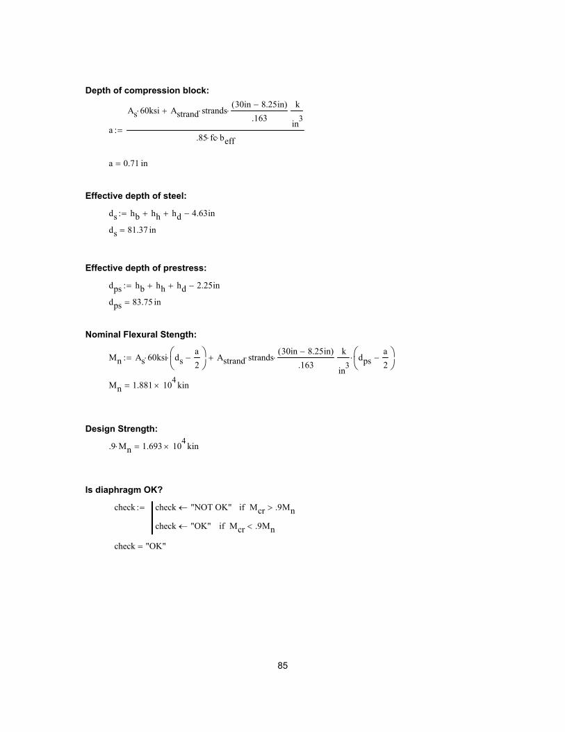
check "OK"=
check check "NOT OK"← Mcr .9Mn>if
check "OK"← Mcr .9Mn<if
:=
Is diaphragm OK?
.9 Mn⋅ 1.693 104
× kin=
Design Strength:
Mn 1.881 104
× kin=
Mn As 60⋅ ksi dsa
2−
⋅ Astrand strands⋅30in 8.25in−( )
.163⋅
k
in3
dpsa
2−
⋅+:=
Nominal Flexural Stength:
dps 83.75 in=
dps hb hh+ hd+ 2.25in−:=
Effective depth of prestress:
ds 81.37 in=
ds hb hh+ hd+ 4.63in−:=
Effective depth of steel:
a 0.71 in=
a
As 60⋅ ksi Astrand strands⋅30in 8.25in−( )
.163⋅
k
in3
+
.85 fc⋅ beff⋅:=
Depth of compression block:
85
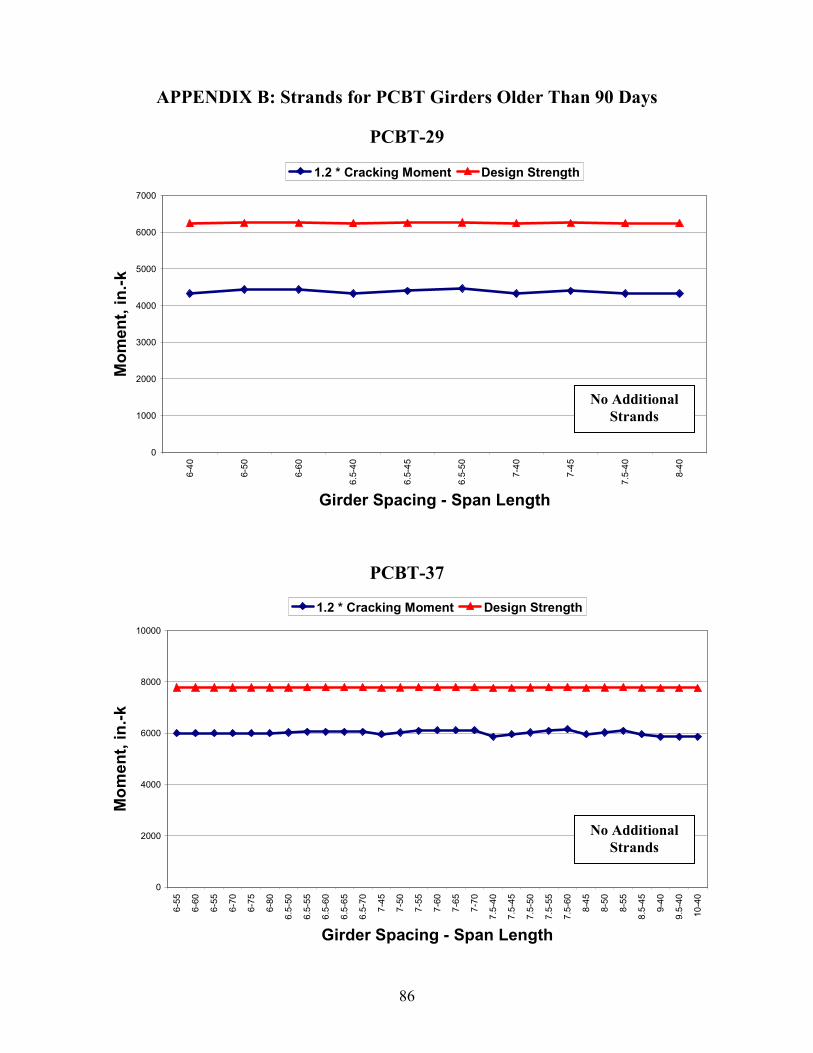
86
APPENDIX B: Strands for PCBT Girders Older Than 90 Days
PCBT-29
0
1000
2000
3000
4000
5000
6000
70006-40
6-50
6-60
6.5-40
6.5-45
6.5-50
7-40
7-45
7.5-40
8-40
Girder Spacing - Span Length
Moment, in.-k
1.2 * Cracking Moment Design Strength
PCBT-37
0
2000
4000
6000
8000
10000
6-55
6-60
6-55
6-70
6-75
6-80
6.5-50
6.5-55
6.5-60
6.5-65
6.5-70
7-45
7-50
7-55
7-60
7-65
7-70
7.5-40
7.5-45
7.5-50
7.5-55
7.5-60
8-45
8-50
8-55
8.5-45
9-40
9.5-40
10-40
Girder Spacing - Span Length
Moment, in.-k
1.2 * Cracking Moment Design Strength
No Additional
Strands
No Additional
Strands
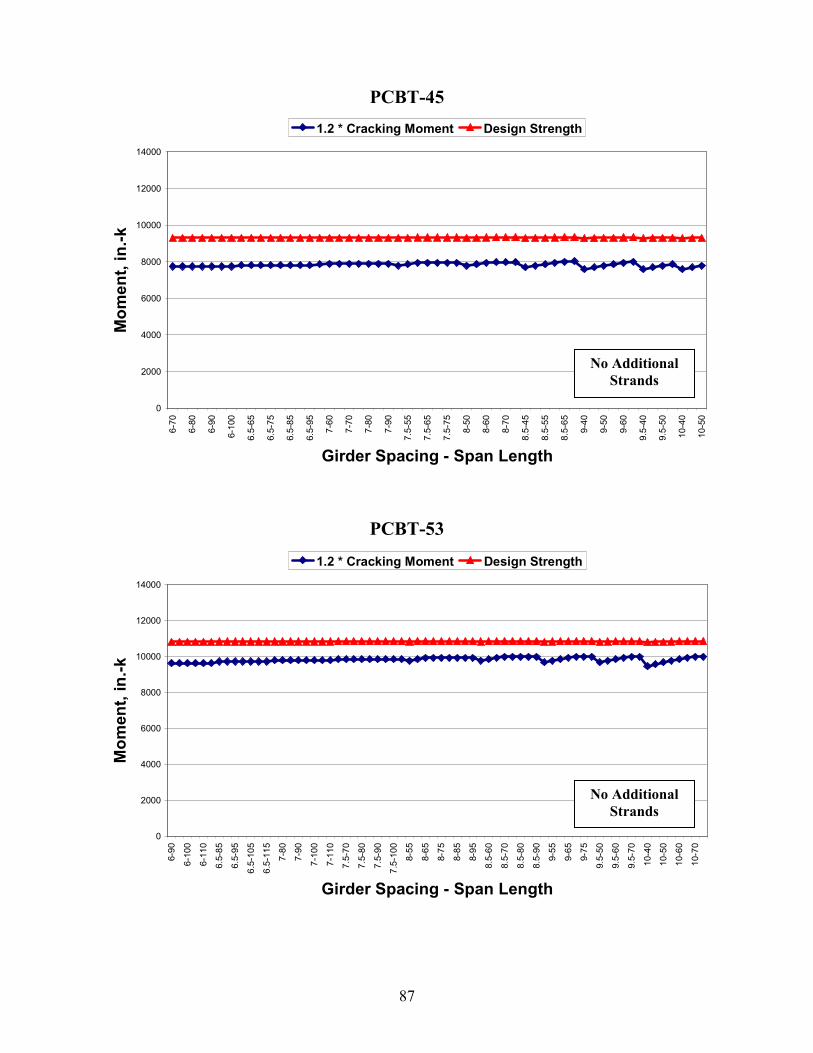
87
PCBT-45
0
2000
4000
6000
8000
10000
12000
14000
6-70
6-80
6-90
6-100
6.5-65
6.5-75
6.5-85
6.5-95
7-60
7-70
7-80
7-90
7.5-55
7.5-65
7.5-75
8-50
8-60
8-70
8.5-45
8.5-55
8.5-65
9-40
9-50
9-60
9.5-40
9.5-50
10-40
10-50
Girder Spacing - Span Length
Moment, in.-k
1.2 * Cracking Moment Design Strength
PCBT-53
0
2000
4000
6000
8000
10000
12000
14000
6-90
6-100
6-110
6.5-85
6.5-95
6.5-105
6.5-115
7-80
7-90
7-100
7-110
7.5-70
7.5-80
7.5-90
7.5-100
8-55
8-65
8-75
8-85
8-95
8.5-60
8.5-70
8.5-80
8.5-90
9-55
9-65
9-75
9.5-50
9.5-60
9.5-70
10-40
10-50
10-60
10-70
Girder Spacing - Span Length
Moment, in.-k
1.2 * Cracking Moment Design Strength
No Additional
Strands
No Additional
Strands
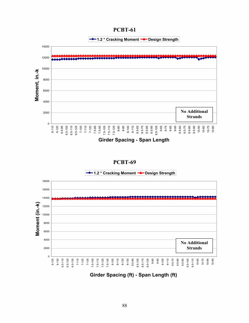
88
PCBT-61
0
2000
4000
6000
8000
10000
12000
14000
6-110
6-120
6.5-95
6.5-105
6.5-115
6.5-125
7-100
7-110
7-120
7.5-85
7.5-95
7.5-105
7.5-115
7.5-125
8-80
8-90
8-100
8-110
8.5-65
8.5-75
8.5-85
8.5-95
8.5-105
9-65
9-75
9-85
9-95
9.5-60
9.5-70
9.5-80
9.5-90
10-50
10-60
10-70
10-80
Girder Spacing - Span Length
Moment, in.-k
1.2 * Cracking Moment Design Strength
PCBT-69
0
2000
4000
6000
8000
10000
12000
14000
16000
18000
6-120
6-130
6.5-115
6.5-125
6.5-135
7-115
7-125
7-135
7.5-105
7.5-115
7.5-125
7.5-135
8-100
8-110
8-120
8-130
8.5-95
8.5-105
8.5-115
8.5-125
9-80
9-90
9-100
9-110
9.5-70
9.5-80
9.5-90
9.5-100
9.5-110
10-65
10-75
10-85
10-95
Girder Spacing (ft) - Span Length (ft)
Moment (in.-k)
1.2 * Cracking Moment Design Strength
No Additional
Strands
No Additional
Strands

89
PCBT-77
0
2000
4000
6000
8000
10000
12000
14000
16000
18000
20000
6-130
6-140
7-130
7-140
7-125
7-135
7-145
8-120
8-130
8-140
8-105
8-115
8-125
8-135
9-100
9-110
9-120
9-130
9-95
9-105
9-115
9-125
10-90
10-100
10-110
10-120
10-80
10-90
10-100
10-110
Girder Spacing - Span Length
Moment, in.-k
1.2 * Cracking Moment Design Strength
PCBT-85
0
2000
4000
6000
8000
10000
12000
14000
16000
18000
20000
22000
24000
6-135
6-145
7-135
7-145
7-130
7-140
7-150
8-130
8-140
8-150
8-125
8-140
8-150
9-120
9-130
9-140
9-150
9-105
9-115
9-125
9-135
9-145
10-105
10-115
10-125
10-135
10-95
10-105
10-115
10-125
Girder Spacing - Span Length
Moment, in.-k
1.2 * Cracking Moment Design Strength
1 Additional
Strand
2 Additional
Strands

90
PCBT-93
0
2000
4000
6000
8000
10000
12000
14000
16000
18000
20000
22000
24000
6-145
6-155
7-145
7-155
7-145
7-155
8-135
8-145
8-155
8-130
8-140
8-150
8-160
9-130
9-140
9-150
9-120
9-130
9-140
9-150
10-110
10-120
10-130
10-140
10-150
10-105
10-115
10-125
10-135
10-145
Girder Spacing - Span Length
Moment, in.-k
1.2 * Cracking Moment Design Strength
2 Additional
Strands

APPENDIX C: 2-Span PCBT Girder Systems Younger than 90 Days
Purpose: Evaluate Continuity Diaphragm Details
sign convention for concrete stresses: " -" for tension, "+" for compression
yellow highlighed regions are input values
UNITS:
k 1000lb:= pcflb
ft3
:=
kft k ft⋅:=µε .000001:=
kin k in⋅:=
psilb
in2
:=ksi
k
in2
:=
klfk
ft:=
91

Ig 443100in4
:=
Distance from centroid to bottom of girder- ygb 29.92in:=
Weight per foot wg wgird Ag⋅:= wg 894.479lb
ft=
Span Length- L 75ft:=
Volume to surface area ratio- vs 3.75in:=
Relative Humidity-H 70:= percent
Deck Properties
Girder spacing- s 10ft:=
Deck depth hf 8.5in:=
Haunch height hh 1.5in:=
Deck concrete fcd 4000psi:=
wdeck 150pcf:=
INPUT:
Time Properties
Age of girder at transfer of prestressing- ti 1:= day
Age of girder at deck placement- td 45:= days
Aging coefficient χ .7:=
Girder Properties
Girder concrete- fc 7000psi:=
fci fc 0.8⋅:= fci 5.6 103
× psi=
wgird 150pcf:=
αTC 6.0 106−
⋅1
F⋅:= (strain per degree F)
Girder height- hg 61in:=
Girder cross-sectional area- Ag 858.7in2
:=
Girder moment of inertia-
92
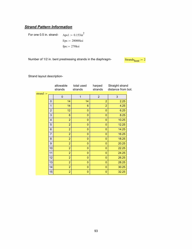
Strand Pattern Information
For one 0.5 in. strand- Aps1 0.153in2
:=
Eps 28000ksi:=
fpu 270ksi:=
Number of 1/2 in. bent prestressing strands in the diaphragm- Strandsbent 2:=
Strand layout description-
allowable total used harped Straight strand
strands strands strands distance from bot.
strand0 1 2 3
0
1
2
3
4
5
6
7
8
9
10
11
12
13
14
15
14 14 2 2.25
14 6 2 4.25
12 0 0 6.25
6 0 0 8.25
2 0 0 10.25
2 0 0 12.25
2 0 0 14.25
2 0 0 16.25
2 0 0 18.25
2 0 0 20.25
2 0 0 22.25
2 0 0 24.25
2 0 0 26.25
2 0 0 28.25
2 0 0 30.25
2 0 0 32.25
:=
93
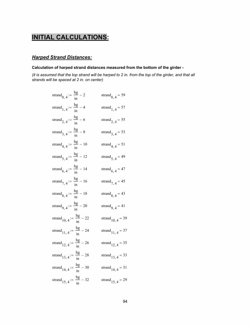
strand7 4,
hg
in16−:= strand
7 4,45=
strand8 4,
hg
in18−:= strand
8 4,43=
strand9 4,
hg
in20−:= strand
9 4,41=
strand10 4,
hg
in22−:= strand
10 4,39=
strand11 4,
hg
in24−:= strand
11 4,37=
strand12 4,
hg
in26−:= strand
12 4,35=
strand13 4,
hg
in28−:= strand
13 4,33=
strand14 4,
hg
in30−:= strand
14 4,31=
strand15 4,
hg
in32−:= strand
15 4,29=
INITIAL CALCULATIONS:
Harped Strand Distances:
Calculation of harped strand distances measured from the bottom of the girder -
(it is assumed that the top strand will be harped to 2 in. from the top of the girder, and that all
strands will be spaced at 2 in. on center)
strand0 4,
hg
in2−:= strand
0 4,59=
strand1 4,
hg
in4−:= strand
1 4,57=
strand2 4,
hg
in6−:= strand
2 4,55=
strand3 4,
hg
in8−:= strand
3 4,53=
strand4 4,
hg
in10−:= strand
4 4,51=
strand5 4,
hg
in12−:= strand
5 4,49=
strand6 4,
hg
in14−:= strand
6 4,47=
94
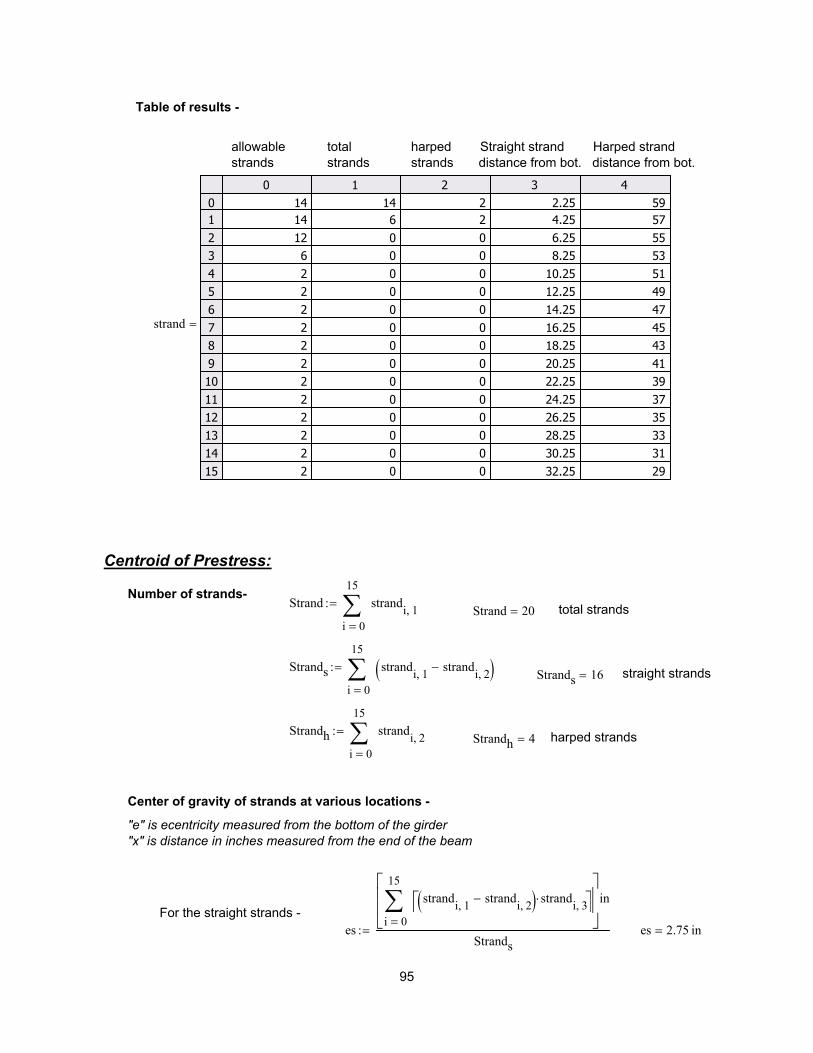
es 2.75 in=es0
15
i
strandi 1,
strandi 2,
−( ) strandi 3,⋅ ∑
=
in
Strands
:=For the straight strands -
"e" is ecentricity measured from the bottom of the girder
"x" is distance in inches measured from the end of the beam
Center of gravity of strands at various locations -
harped strandsStrandh 4=Strandh
0
15
i
strandi 2,∑
=
:=
straight strandsStrands 16=Strands
0
15
i
strandi 1,
strandi 2,
−( )∑=
:=
total strandsStrand 20=Strand
0
15
i
strandi 1,∑
=
:=Number of strands-
Centroid of Prestress:
strand
0 1 2 3 4
0
1
2
3
4
5
6
7
8
9
10
11
12
13
14
15
14 14 2 2.25 59
14 6 2 4.25 57
12 0 0 6.25 55
6 0 0 8.25 53
2 0 0 10.25 51
2 0 0 12.25 49
2 0 0 14.25 47
2 0 0 16.25 45
2 0 0 18.25 43
2 0 0 20.25 41
2 0 0 22.25 39
2 0 0 24.25 37
2 0 0 26.25 35
2 0 0 28.25 33
2 0 0 30.25 31
2 0 0 32.25 29
=
allowable total harped Straight strand Harped strand
strands strands strands distance from bot. distance from bot.
Table of results -
95

cgshp 2.85 in=cgshp
es Strands⋅ ehhp Strandh⋅+
Strand:=
ehhp 3.25 in=ehhp ehend
ehend ehms−( ).4 L⋅
x⋅−:=x .4 L⋅:=
For harped stands at the harping point -
cgs.5hp 8.325 in=cgs.5hp
es Strands⋅ eh.5hp Strandh⋅+
Strand:=
eh.5hp 30.625 in=eh.5hp ehend
ehend ehms−( ).4 L⋅
x⋅−:=x .2 L⋅:=
For harped stands at 1/2 the distance to the harping point -
cgstl 13.04 in=cgstl
es Strands⋅ ehtl Strandh⋅+
Strand:=
ehtl 54.198 in=ehtl ehend
ehend ehms−( ).4 L⋅
x⋅−:=x 25in:=
For harped strand at the transfer length -
cgsend 13.8 in=cgsend
es Strands⋅ ehend Strandh⋅+
Strand:=
ehend 58 in=ehend0
15
i
strandi 2,
strandi 4,
⋅( )∑=
in
Strandh
:=x 0in:=
For harped strands at the ends -
cgsms 2.85 in=cgsms
es Strands⋅ ehms Strandh⋅+
Strand:=
ehms 3.25 in=ehms0
15
i
strandi 2,
strandi 3,
⋅( )∑=
in
Strandh
:=x .5 L⋅:=
For harped stands at mid span -
96
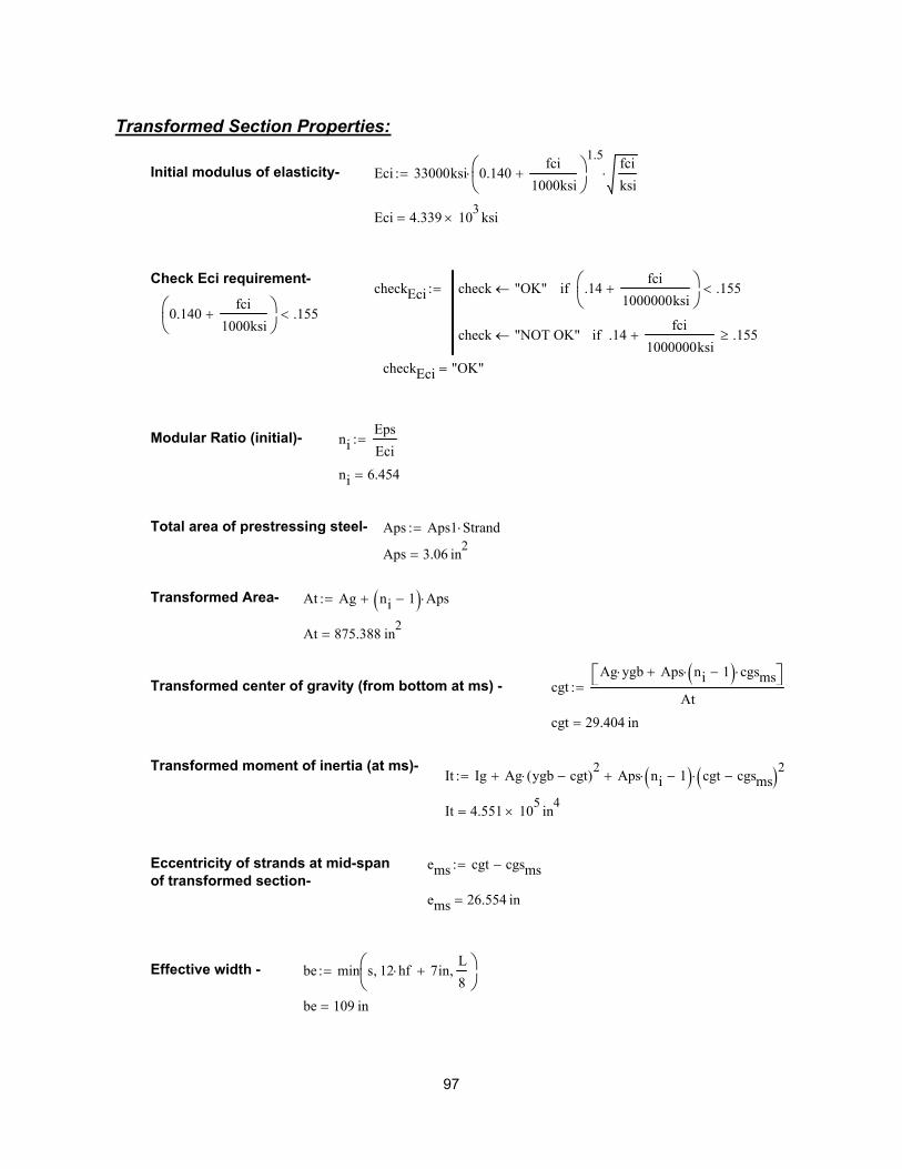
be 109 in=
be min s 12 hf⋅ 7in+,L
8,
:=Effective width -
ems 26.554 in=
ems cgt cgsms−:=Eccentricity of strands at mid-span
of transformed section-
It 4.551 105
× in4
=
It Ig Ag ygb cgt−( )2
⋅+ Aps ni 1−( )⋅ cgt cgsms−( )2⋅+:=Transformed moment of inertia (at ms)-
cgt 29.404 in=
cgtAg ygb⋅ Aps ni 1−( )⋅ cgsms⋅+
At:=Transformed center of gravity (from bottom at ms) -
At 875.388 in2
=
At Ag ni 1−( ) Aps⋅+:=Transformed Area-
Aps 3.06 in2
=
Aps Aps1 Strand⋅:=Total area of prestressing steel-
ni 6.454=
niEps
Eci:=Modular Ratio (initial)-
checkEci "OK"=
0.140fci
1000ksi+
.155<
checkEci check "OK"← .14fci
1000000ksi+
.155<if
check "NOT OK"← .14fci
1000000ksi+ .155≥if
:=Check Eci requirement-
Eci 4.339 103
× ksi=
Eci 33000ksi 0.140fci
1000ksi+
1.5
⋅fci
ksi⋅:=Initial modulus of elasticity-
Transformed Section Properties:
97
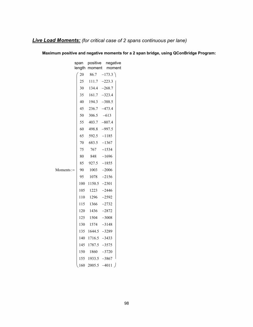
Live Load Moments: (for critical case of 2 spans continuous per lane)
Maximum positive and negative moments for a 2 span bridge, using QConBridge Program:
span positive negative
length moment moment
Moments
20
25
30
35
40
45
50
55
60
65
70
75
80
85
90
95
100
105
110
115
120
125
130
135
140
145
150
155
160
86.7
111.7
134.4
161.7
194.3
236.7
306.5
403.7
498.8
592.5
683.5
767
848
927.5
1003
1078
1150.5
1223
1296
1366
1436
1504
1574
1644.5
1716.5
1787.5
1860
1933.5
2005.5
173.3−
223.3−
268.7−
323.4−
388.5−
473.4−
613−
807.4−
997.5−
1185−
1367−
1534−
1696−
1855−
2006−
2156−
2301−
2446−
2592−
2732−
2872−
3008−
3148−
3289−
3433−
3575−
3720−
3867−
4011−
:=
98
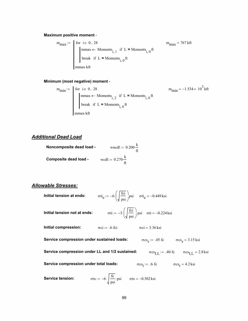
σti 3−fci
psi
⋅ psi⋅:= σti 0.224− ksi=
Initial compression: σci .6 fci⋅:= σci 3.36 ksi=
Service compression under sustained loads: σcss .45 fc⋅:= σcss 3.15 ksi=
Service compression under LL and 1/2 sustained: σcsLL .40 fc⋅:= σcsLL 2.8 ksi=
Service compression under total loads: σcst .6 fc⋅:= σcst 4.2 ksi=
Service tension: σts 6−fc
psi⋅ psi⋅:= σts 0.502− ksi=
Maximum positive moment -
mmax
mmax Momentsi 1,
← L Momentsi 0,
ft=if
break L Momentsi 0,
ft=if
i 0 28..∈for
mmax kft⋅
:= mmax 767 kft=
Minimum (most negative) moment -
mmin
mmax Momentsi 2,
← L Momentsi 0,
ft=if
break L Momentsi 0,
ft=if
i 0 28..∈for
mmax kft⋅
:= mmin 1.534− 103
× kft=
Additional Dead Load
Noncomposite dead load - wncdl 0.200k
ft:=
Composite dead load - wcdl 0.270k
ft:=
Allowable Stresses:
Initial tension at ends: σtie 6fci
psi
⋅ psi−:= σtie 0.449− ksi=
Initial tension not at ends:
99
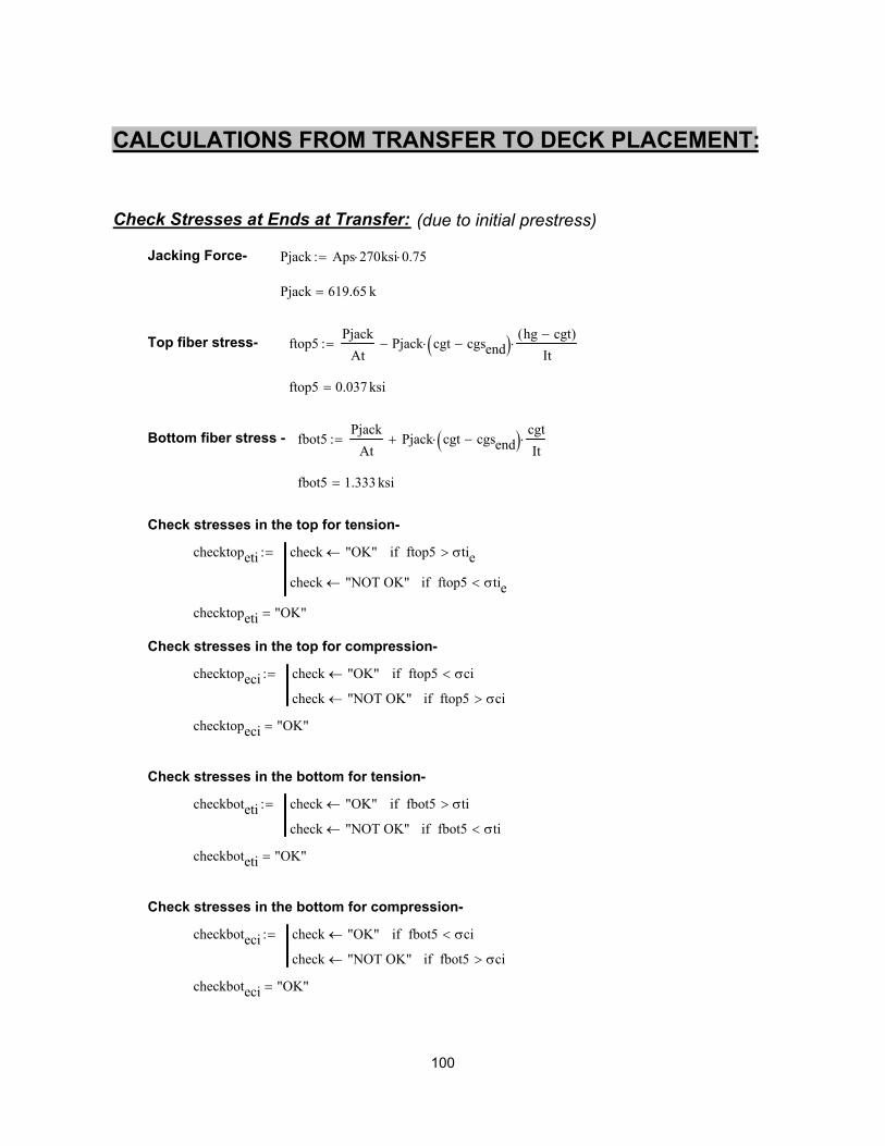
checkboteci "OK"=
checkboteci check "OK"← fbot5 σci<if
check "NOT OK"← fbot5 σci>if
:=
Check stresses in the bottom for compression-
checkboteti "OK"=
checkboteti check "OK"← fbot5 σti>if
check "NOT OK"← fbot5 σti<if
:=
Check stresses in the bottom for tension-
checktopeci "OK"=
checktopeci check "OK"← ftop5 σci<if
check "NOT OK"← ftop5 σci>if
:=
Check stresses in the top for compression-
checktopeti "OK"=
checktopeti check "OK"← ftop5 σtie>if
check "NOT OK"← ftop5 σtie<if
:=
Check stresses in the top for tension-
fbot5 1.333ksi=
fbot5Pjack
AtPjack cgt cgsend−( )⋅
cgt
It⋅+:=Bottom fiber stress -
ftop5 0.037ksi=
ftop5Pjack
AtPjack cgt cgsend−( )⋅
hg cgt−( )
It⋅−:=Top fiber stress-
Pjack 619.65 k=
Pjack Aps 270⋅ ksi 0.75⋅:=Jacking Force-
Check Stresses at Ends at Transfer: (due to initial prestress)
CALCULATIONS FROM TRANSFER TO DECK PLACEMENT:
100
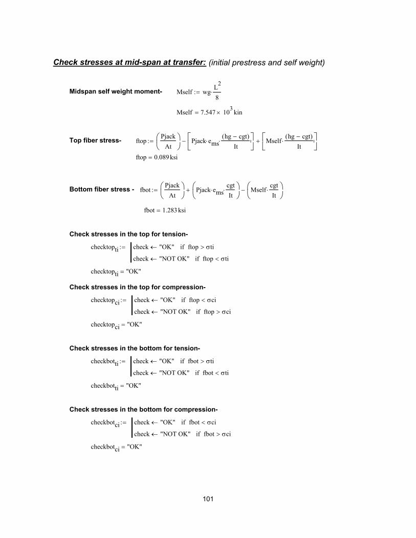
checkbotci "OK"=
checkbotci check "OK"← fbot σci<if
check "NOT OK"← fbot σci>if
:=
Check stresses in the bottom for compression-
checkbotti "OK"=
checkbotti check "OK"← fbot σti>if
check "NOT OK"← fbot σti<if
:=
Check stresses in the bottom for tension-
checktopci "OK"=
checktopci check "OK"← ftop σci<if
check "NOT OK"← ftop σci>if
:=
Check stresses in the top for compression-
checktopti "OK"=
checktopti check "OK"← ftop σti>if
check "NOT OK"← ftop σti<if
:=
Check stresses in the top for tension-
fbot 1.283ksi=
fbotPjack
At
Pjack ems⋅cgt
It⋅
+ Mselfcgt
It⋅
−:=Bottom fiber stress -
ftop 0.089ksi=
ftopPjack
At
Pjack ems⋅hg cgt−( )
It⋅
− Mselfhg cgt−( )
It⋅
+:=Top fiber stress-
Mself 7.547 103
× kin=
Mself wgL2
8⋅:=Midspan self weight moment-
Check stresses at mid-span at transfer: (initial prestress and self weight)
101

ψbif 1.385=
ψbif 1.9 klai⋅ ks⋅ khc⋅ kf⋅:=Girder creep at end of service due
to loading introduced at transfer-
epg 27.07 in=
epg ygb cgsms−:=Eccentricity of strands with respect to
gross section properties-
εbid 1.863 104−
×=
εbid 480 106−
⋅ ktd⋅ ks⋅ khs⋅ kf⋅:=Shrinkage from transfer to deck placement-
Shrinkage of Girder Concrete: (from transfer to deck placement)
khc 1=
khc 1.56 0.008 H⋅−:=Humidity factor for creep-
klai 1=
klai ti0.118−
:=Loading age factor-
kf 0.758=
kf5
1fci
ksi+
:=Concrete strength factor-
khs 0.999=
khs 2.00 0.0143 H⋅−:=Humidity factor for shrinkage-
ks 0.963=
ks 1.45 .13vs
in⋅−:=Girder Size factor-
ktd 0.533=
ktdtd ti−
61 4fci
ksi⋅− td ti−( )+
:=Time development factor-
Factors for Time Dependent Effects:
102

checkfpo "OK"=
checkfpo check "OK"← fpo .55 fpy⋅>if
check "NOT OK"← fpo .55 fpy⋅<if
:=
Note: fpo > .55 fpyCheck requirement -
fpy 243 ksi=
fpy 0.90 270⋅ ksi:=Yield stress-
fpo 194.578 ksi=
fpo 0.75 270⋅ ksi fcgp ni⋅−:=Initial stress in strand after transfer-
Relaxation of Prestressing Strands: (from transfer to deck placement)
∆fpCR 5.269ksi=
∆fpCR ni fcgp⋅ ψbid⋅ Kid⋅:=Prestress loss due to creep
from transfer to deck placement-
fcgp 1.228ksi=
fcgpPjack
AtPjack
ems2
It⋅+ Mself
ems
It⋅−:=Concrete stress at centroid of strand due to
initial prestress plus self weight of girder-
ψbid 0.738=
ψbid 1.90 ktd⋅ klai⋅ ks⋅ khc⋅ kf⋅:=Girder creep coefficient at time of deck
placement due to loading introduced at transfer-
Creep of Girder Concrete: (from transfer to deck placement)
∆fpSR 4.7 ksi=
∆fpSR εbid Eps⋅ Kid⋅:=Prestress Loss due to shrinkage
from transfer to deck placement-
Kid 0.901=
Kid1
1 niAps
Ag⋅ 1
Ag epg( )2
⋅
Ig+
⋅ 1 χ ψbif⋅+( )⋅+
:=Transformed section coefficient
(between initial and deck placement)-
103

Inherent relaxation-Li
fpo
45
fpo
fpy0.55−
⋅ log24 td⋅( )24( )
⋅:=(It is assume that the age of concrete
at transfer of prestressing is 1 day) Li 1.792ksi=
Reduction factor for relaxation losses- φi 13 ∆fpSR ∆fpCR+( )⋅
fpo−:=
φi 0.846=
Prestress Loss due to relaxation of prestressing
strands from transfer to deck placement-∆fpR1 φi Li⋅ Kid⋅:=
∆fpR1 1.367ksi=
Prestress at time of deck placement- fpd fpo ∆fpSR− ∆fpCR− ∆fpR1−:=
fpd 183.242 ksi=
104
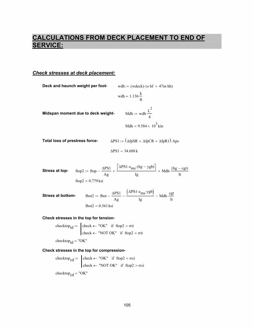
checktopcd "OK"=
checktopcd check "OK"← ftop2 σci<if
check "NOT OK"← ftop2 σci>if
:=
Check stresses in the top for compression-
checktoptd "OK"=
checktoptd check "OK"← ftop2 σti>if
check "NOT OK"← ftop2 σti<if
:=
Check stresses in the top for tension-
fbot2 0.561ksi=
fbot2 fbot∆PS1
Ag−
∆PS1 ems⋅ ygb⋅( )Ig
− Mdhcgt
It⋅−:=Stress at bottom-
ftop2 0.779ksi=
ftop2 ftop∆PS1
Ag−
∆PS1 ems⋅ hg ygb−( )⋅ Ig
+ Mdhhg cgt−( )
It⋅+:=Stress at top-
∆PS1 34.688 k=
∆PS1 ∆fpSR ∆fpCR+ ∆fpR1+( ) Aps⋅:=Total loss of prestress force-
Mdh 9.584 103
× kin=
Mdh wdhL2
8⋅:=Midspan moment due to deck weight-
wdh 1.136k
ft=
wdh wdeck( ) s hf⋅ 47in hh⋅+( )⋅:=Deck and haunch weight per foot-
Check stresses at deck placement:
CALCULATIONS FROM DECK PLACEMENT TO END OFSERVICE:
105
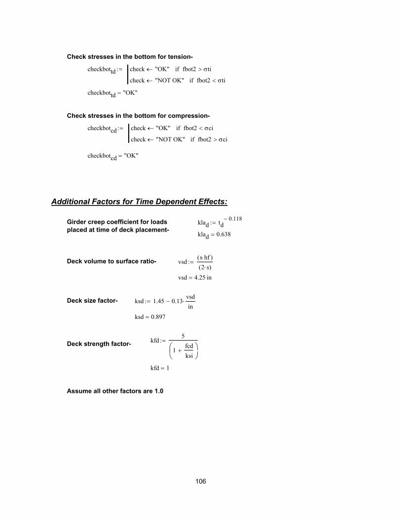
Assume all other factors are 1.0
kfd 1=
Deck strength factor-kfd
5
1fcd
ksi+
:=
ksd 0.897=
ksd 1.45 0.13vsd
in⋅−:=Deck size factor-
vsd 4.25 in=
vsds hf⋅( )
2 s⋅( ):=Deck volume to surface ratio-
klad 0.638=
klad td0.118−
:=Girder creep coefficient for loads
placed at time of deck placement-
Additional Factors for Time Dependent Effects:
checkbotcd "OK"=
checkbotcd check "OK"← fbot2 σci<if
check "NOT OK"← fbot2 σci>if
:=
Check stresses in the bottom for compression-
checkbottd "OK"=
checkbottd check "OK"← fbot2 σti>if
check "NOT OK"← fbot2 σti<if
:=
Check stresses in the bottom for tension-
106

Act 1.604 103
× in2
=
Act Agc ns 1−( ) Aps⋅+:=Transformed composite area-
ns 5.69=
nsEps
Ec:=Modular ratio for prestressing strands to girder concrete-
Calculate transformed composite cross-sectional properties:
Igc 9.737 105
× in4
=
Igc Ig Ag ygb cggc−( )2
⋅+1
12be⋅ hf
3⋅ nd⋅+ be hf⋅ nd⋅ hg hh+
hf
2+ cggc−
2
⋅+
1
1247⋅ in hh
3⋅ nd⋅ 47in hh⋅ nd⋅ hg
hh
2+ cggc−
2
⋅+
+
...:=
Moment of Inertia of Gross Composite Area-
cggc 46.69 in=
cggc
Ag ygb⋅ hf be⋅ hg hh+hf
2+
⋅ nd⋅+ hh 47⋅ in hghh
2+
⋅ nd⋅+
Agc:=
Centroid (from bottom) of
Gross Composite Area-
Agc 1.589 103
× in2
=
Agc Ag hf be⋅ hh 47⋅ in+( ) nd⋅+:=Gross composite area-
nd 0.733=
ndEcd
Ec:=Modular ratio for deck to girder concrete-
Ecd 3.607 103
× ksi=
Ecd 33000ksi 0.140fcd
1000ksi+
1.5
⋅fcd
ksi⋅:=Modulus for Deck Concrete at 28 days-
Ec 4.921 103
× ksi=
Ec 33000ksi 0.140fc
1000ksi+
1.5
⋅fc
ksi⋅:=Modulus of Girder Concrete at 28 days-
Calculate the Gross Composite Section Properties:
107

wcdl 0.27k
ft=Permanent load on composite section
(from VDOT design standards)-
ψbdf 0.884=
ψbdf 1.9 klad⋅ ks⋅ khc⋅ kf⋅:=Girder creep for loads placed at
time of deck placement-
ψddf 1.292=
ψddf 1.9 ksd⋅ khc⋅ kf⋅:=Creep of deck concrete from time of
deck placement to end of service-
∆fpCD1 4.709ksi=
∆fpCD1 ni fcgp⋅ ψbif ψbid−( )⋅ Kdf⋅:=Prestress loss due to initial prestress
and self weight of girder-
Creep of girder concrete: (from deck placement to end of service)
∆fpSD 4.2 ksi=
∆fpSD εbdf Eps⋅ Kdf⋅:=Prestress loss due to shrinkage from
deck placement to end of service-
Kdf 0.918=
Kdf1
1 nsAps
Agc⋅ 1
Agc cggc cgsms−( )2⋅
Igc+
⋅ 1 χ ψbif⋅+( )⋅+
:=
Transformed section coefficient (between deck placement and final time)-
εbdf 1.634 104−
×=
εbdf εbif εbid−:=Shrinkage from deck placement to end of service-
εbif 3.496 104−
×=
εbif 480 106−
⋅ ks⋅ khs⋅ kf⋅:=Shrinkage from transfer to end of service-
Shrinkage of girder concrete: (from deck placement to end of service)
Ict 1.001 106
× in4
=
Ict Igc Agc cggc cgct−( )2
⋅+ Aps ns 1−( )⋅ cgct cgsms−( )2⋅+:=Moment of inertia of transformed
composite area-
cgct 46.297 in=
cgctAgc cggc⋅ Aps ns 1−( )⋅ cgsms⋅+
Act:=Centroid of transformed composite area-
108

∆fpR2 1.367ksi=
∆fpR2 ∆fpR1:=Prestress Loss due to relaxation of prestressing
strands from deck placement to end of service-
Relaxation of Prestressing Strands: (from deck placement to end of service)
∆fpCD 0.991ksi=
∆fpCD ∆fpCD1 ∆fpCD2+:=Total creep of girder concrete-
∆fpCD2 3.717− ksi=
∆fpCD2 ns ∆fccs ∆fcdp+ ∆fcl+( )⋅ ψbdf⋅ Kdf⋅:=Prestress loss due to placement of deck-
∆fcl 0.098− ksi=
∆fcl ∆fpSR ∆fpCR+ ∆fpR1+( )−Aps
Ag⋅ 1
Ag epg2
⋅
Ig+
⋅:=Change in stress in concrete at level
of strand due long term losses
between initial and deck placement-
∆fcdp 0.658− ksi=
∆fcdp Mdh Mncomp+( )−ems
It⋅:=Change in stress in concrete at level
of strand due to deck placement-
∆fccs 0.049− ksi=
∆fccs Mcomp−cgct cgsms−( )
Ict⋅:=Change in stress in concrete at level of strand due
to superimposed loads on composite section-
Mncomp 1.688 103
× kin=
Mncomp wncdlL2
8⋅:=Moment from permanent non-composite DL-
(at mid-span)
wncdl 0.2k
ft=Permanent load on non-composite
section (from VDOT Standards)-
Mcomp 1.139 103
× kin=
Mcomp wcdlL2
16⋅:=Moment from permanent composite DL-
(at mid-span)
109
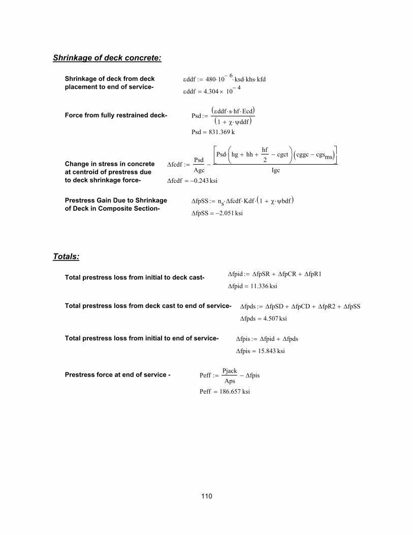
Peff 186.657 ksi=
PeffPjack
Aps∆fpis−:=Prestress force at end of service -
∆fpis 15.843 ksi=
∆fpis ∆fpid ∆fpds+:=Total prestress loss from initial to end of service-
∆fpds 4.507ksi=
∆fpds ∆fpSD ∆fpCD+ ∆fpR2+ ∆fpSS+:=Total prestress loss from deck cast to end of service-
∆fpid 11.336 ksi=Total prestress loss from initial to deck cast-
∆fpid ∆fpSR ∆fpCR+ ∆fpR1+:=
Totals:
∆fpSS 2.051− ksi=
∆fpSS ns ∆fcdf⋅ Kdf⋅ 1 χ ψbdf⋅+( )⋅:=Prestress Gain Due to Shrinkage
of Deck in Composite Section-
∆fcdf 0.243− ksi=
∆fcdfPsd
Agc
Psd hg hh+hf
2+ cgct−
⋅ cggc cgsms−( )⋅
Igc−:=Change in stress in concrete
at centroid of prestress due
to deck shrinkage force-
Psd 831.369 k=
Psdεddf s⋅ hf⋅ Ecd⋅( )1 χ ψddf⋅+( ):=Force from fully restrained deck-
εddf 4.304 104−
×=
εddf 480 106−
⋅ ksd⋅ khs⋅ kfd⋅:=Shrinkage of deck from deck
placement to end of service-
Shrinkage of deck concrete:
110
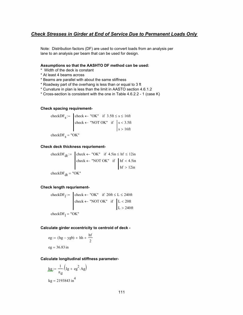
kg 2193843 in4
=
kg1
nd
Ig eg2Ag⋅+( )⋅:=
Calculate longitudinal stiffness parameter-
eg 36.83 in=
eg hg ygb−( ) hh+hf
2+:=
Calculate girder eccentricity to centroid of deck -
checkDFl "OK"=
checkDFl check "OK"← 20ft L≤ 240ft≤if
check "NOT OK"← L 20ft<
L 240ft>
if
:=
Check length requriement-
checkDFdt "OK"=
checkDFdt check "OK"← 4.5in hf≤ 12in≤if
check "NOT OK"← hf 4.5in<
hf 12in>
if
:=
Check deck thickness requriement-
checkDFs "OK"=
checkDFs check "OK"← 3.5ft s≤ 16ft≤if
check "NOT OK"← s 3.5ft<
s 16ft>
if
:=
Check spacing requirement-
Assumptions so that the AASHTO DF method can be used:
* Width of the deck is constant
* At least 4 beams across
* Beams are parallel with about the same stiffness
* Roadway part of the overhang is less than or equal to 3 ft
* Curvature in plan is less than the limit in AASTO section 4.6.1.2
* Cross-section is consistent with the one in Table 4.6.2.2 - 1 (case K)
Note: Distribution factors (DF) are used to convert loads from an analysis per
lane to an analysis per beam that can be used for design.
Check Stresses in Girder at End of Service Due to Permanent Loads Only
111

M.5LL 664− kft=M.5LL Mmin .5⋅:=
Live load moments per beam-
Mmin 1329− kft=Mmin mmin DF⋅:=
Mmax 664 kft=Mmax mmax DF⋅:=
Live load moments per beam-
DF 0.866=
DF DF DF1← DF1 DF2>if
DF DF2← DF1 DF2<if
:=
The controlling DF is the larger of the 2 distribution factors-
DF2 0.866=
DF2 0.075s
9.5ft
.6s
L
.2
⋅kg
L hf3
⋅
.1
⋅+:=
DF for Moment for 2 lane loaded -
DF1 0.608=
DF1 0.06s
14ft
.4s
L
.3
⋅kg
L hf3
⋅
.1
⋅+:=
DF for Moment for 1 lane loaded -
checkDFkg "OK"=
checkDFkg check "OK"← 10000in4
kg≤ 7000000in4
≤if
check "NOT OK"← kg 10000in4
<
kg 7000000in4
>
if
:=
Check longitudinal stiffness requirement-
112

Calculate Cracking Moment
Calculate Cracking Moment of the Continuity Diaphragm:
Tensile strength of Diaphragm Concrete- fr 7.5psifcd
psi:=
fr 474.342 psi=
Cracking Moment- Mcr frIgc
cggc⋅:=
Mcr 824.3 kft=
113

θp 5.137 103−
×=
θp θps θph+:=Total initial end rotation-
θph 5.608 104−
×=
θph
Peff Aps⋅Strandh
Strand⋅
.3 cggc ehms−( )⋅ .2 ehend cggc−( )⋅− ⋅ L( )⋅
Eci It⋅
:=
Initial end rotation from prestress (Harped strands only)-
Note: The moment arm is the center of gravity of the gross composite section - not the
transformed. So, the effective prestressing force should have the elastic shortening removed.
θps 0.0046=
(Straight strands only) θps
Peff Aps⋅Strands
Strand⋅
cggc es−( )⋅ L( )⋅
2 Eci⋅ It⋅
:=Initial end rotation from prestress -
Calculate moment to restrain rotation due to initial prestress:
MφDLR 698.686 kft=
MφDLR
3 θcr⋅ Eci It⋅( )⋅
L 1 χ ψbif ψbid−( )⋅+ ⋅:=Moment to restrain dead load creep rotation -
1
1 χψ+Modify the creep rotation by using:
radiansθcr 1.851 103−
×=
θcr ψbif ψbid−( ) wg wdh+ wncdl+( ) L3
⋅
24 Eci⋅ It⋅⋅:=Creep rotation after continuity -
MDLR 1.568 103
× kft=
MDLRwg wdh+ wncdl+( ) L
2⋅
8:=Dead load restraint moment to restore rotation to zero -
Calculate moment to restrain creep rotation due to dead load:
Calculate Time Dependent Moments in Diaphragm
114

MφPSloss 46.816 kft=
MφPSloss MPSloss1
1 χ ψbif ψbid−( )⋅+⋅:=Modified remaining prestress
restraint moment losses -
MPSloss 68.033 kft=
MPSloss 1 %lossesd−( ) ∆MPSR⋅:=Remaining prestress restraint moment losses -
MφPSR 1.285 103
× kft=
MφPSR MPSRdψbif ψbid−( )
1 χ ψbif ψbid−( )⋅+⋅:=Modified prestress restraint moment caused by
creep rotations at time of deck placement-
MPSRd 2.885 103
× kft=
MPSRd MPSRi %lossesd ∆MPSR⋅−:=Prestress restraint moment at time of deck placement -
%lossesd 0.715=
%lossesd∆fpid
∆fpis:=Percent of total losses at time of deck placement -
∆MPSR 239.127 kft=
∆MPSR MPSRi MPSR−:=Losses in prestress restraint moment -
MPSRi 3.056 103
× kft=
MPSRi MPSRPjack
Peff Aps⋅⋅:=Prestress restraint moment without losses -
MPSR 2.817 103
× kft=
MPSR3 θp⋅ Eci It⋅( )⋅
L:=Restraint moment to restore prestress rotation to zero -
115

MTD 961.852− kft=
MTD MφDLR− MφPSR+ MφDSR− MφPSloss−:=
Calculate final time dependent moments:
MφDSR 1.502 103
× kft=
MφDSR
Mdiffrest
1 χ ψbdf⋅+:=
Modified moment for creep relaxation -
Mdiffrest 2.431 103
× kft=
Mdiffrest Mdiffsh 1.5⋅:=Check differential shrinkage restraint moment -
Mdiffsh 1.621 103
× kft=
Mdiffsh Fdiffsh hg cggc− hh+cgdiffsh
2+
⋅:=Differential shrinkage moment -
cgdiffsh 5.427 in=
cgdiffsh
hf s⋅ hhhf
2+
⋅ hh 47⋅ inhh
2
⋅+
hf s⋅ hh 47⋅ in+:=
Centroid of differential shrinkage force -
Fdiffsh 1.05 103
× k=(applied at centroid of deck and haunch)
Fdiffsh εdiffsh hf s⋅ hh 47⋅ in+( )⋅ Ecd⋅:=Differential shrinkage force -
εdiffsh 2.67 104−
×=
εdiffsh εddf εbdf−:=Differential shrinkage from deck placement to end of service -
Calculate moment to restrain rotation due to differential shrinkage:
116
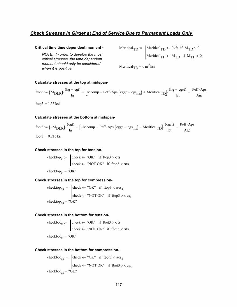
checkbotcs "OK"=
checkbotcs check "OK"← fbot3 σcss<if
check "NOT OK"← fbot3 σcss>if
:=
Check stresses in the bottom for compression-
checkbotts "OK"=
checkbotts check "OK"← fbot3 σts>if
check "NOT OK"← fbot3 σts<if
:=
Check stresses in the bottom for tension-
checktopcs "OK"=
checktopcs check "OK"← ftop3 σcss<if
check "NOT OK"← ftop3 σcss>if
:=
Check stresses in the top for compression-
checktopts "OK"=
checktopts check "OK"← ftop3 σts>if
check "NOT OK"← ftop3 σts<if
:=
Check stresses in the top for tension-
fbot3 0.216ksi=
fbot3 MDLR−( ) cgt( )
Ig⋅ Mcomp− Peff Aps⋅ cggc cgsms−( )⋅+ McriticalTD−
cgct( )
Ict⋅+
Peff Aps⋅
Agc+:=
Calculate stresses at the bottom at midspan-
ftop3 1.35 ksi=
ftop3 MDLR( ) hg cgt−( )
Ig⋅ Mcomp Peff Aps⋅ cggc cgsms−( )⋅− McriticalTD+
hg cgct−( )
Ict⋅+
Peff Aps⋅
Agc+:=
Calculate stresses at the top at midspan-
McriticalTD 0m3ksi=
NOTE: In order to develop the most
critical stresses, the time dependent
moment should only be considered
when it is positive.
McriticalTD McriticalTD 0kft← MTD 0≤if
McriticalTD MTD← MTD 0>if
:=Critical time time dependent moment -
Check Stresses in Girder at End of Service Due to Permanent Loads Only
117
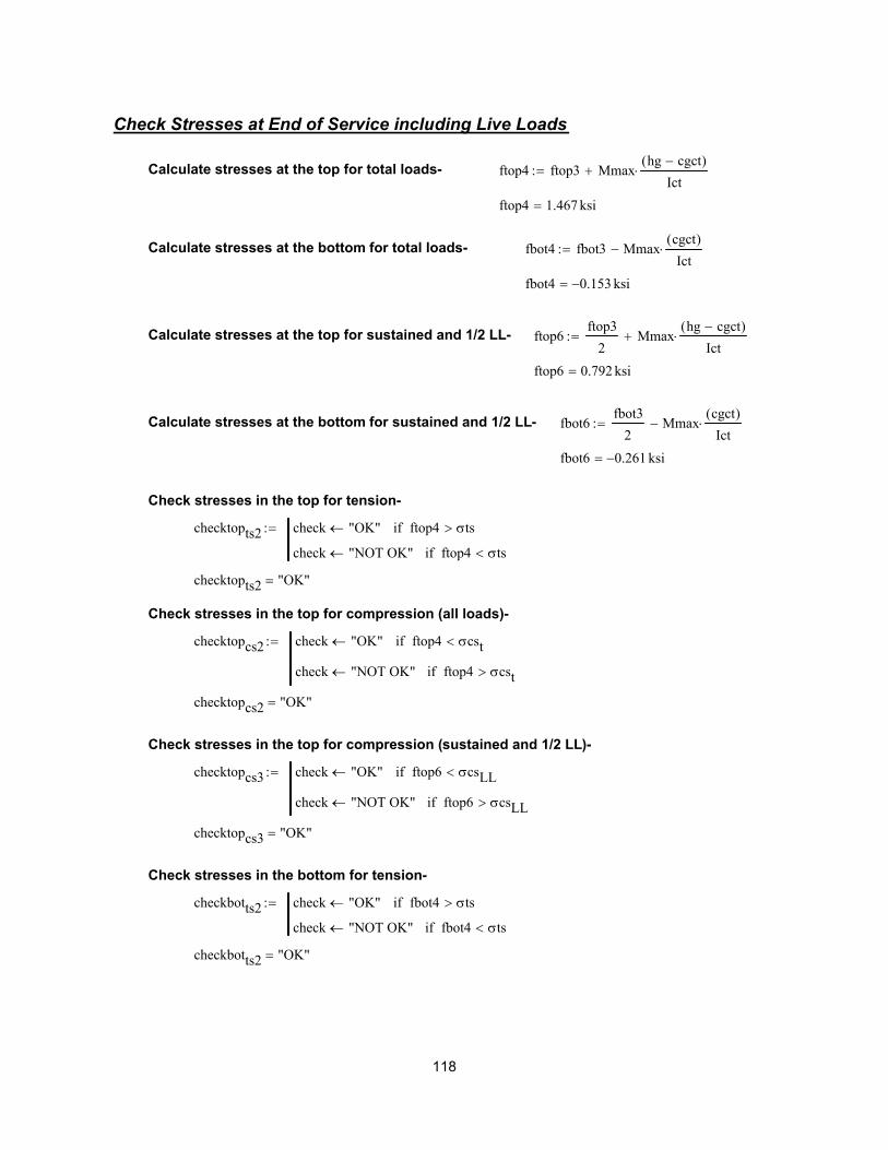
checkbotts2 "OK"=
checkbotts2 check "OK"← fbot4 σts>if
check "NOT OK"← fbot4 σts<if
:=
Check stresses in the bottom for tension-
checktopcs3 "OK"=
checktopcs3 check "OK"← ftop6 σcsLL<if
check "NOT OK"← ftop6 σcsLL>if
:=
Check stresses in the top for compression (sustained and 1/2 LL)-
checktopcs2 "OK"=
checktopcs2 check "OK"← ftop4 σcst<if
check "NOT OK"← ftop4 σcst>if
:=
Check stresses in the top for compression (all loads)-
checktopts2 "OK"=
checktopts2 check "OK"← ftop4 σts>if
check "NOT OK"← ftop4 σts<if
:=
Check stresses in the top for tension-
fbot6 0.261− ksi=
fbot6fbot3
2Mmax
cgct( )
Ict⋅−:=Calculate stresses at the bottom for sustained and 1/2 LL-
ftop6 0.792ksi=
ftop6ftop3
2Mmax
hg cgct−( )
Ict⋅+:=Calculate stresses at the top for sustained and 1/2 LL-
fbot4 0.153− ksi=
fbot4 fbot3 Mmaxcgct( )
Ict⋅−:=Calculate stresses at the bottom for total loads-
ftop4 1.467ksi=
ftop4 ftop3 Mmaxhg cgct−( )
Ict⋅+:=Calculate stresses at the top for total loads-
Check Stresses at End of Service including Live Loads
118

Check stresses in the bottom for compression (all loads)-
checkbotcs2 check "OK"← fbot4 σcst<if
check "NOT OK"← fbot4 σcst>if
:=
checkbotcs2 "OK"=
Check stresses in the bottom for compression (sustained and 1/2 LL)-
checkbotcs3 check "OK"← fbot6 σcsLL<if
check "NOT OK"← fbot6 σcsLL>if
:=
checkbotcs3 "OK"=
Note: For the loading condition with with the live load, the stresses for the top are checked using
Service I and stresses for the bottom are checked using Service III (for the tension check).
119

P6 0.122k=P6TD
2
11in 7in+( )
2in⋅ 2⋅ Ec⋅ αTC⋅:=
(assume that TE is very small, so just take the average of TD and TE for P6)TE 0:=
P5 1.654k=P5 17.25in TD⋅ 26.25in TC⋅+( )in Ec⋅ αTC⋅:=
TD 0.458F=TD 11F hf hh+ 4in− 4in+ 1.5in+( )11
12⋅
F
in⋅−:=
P4 20.353 k=P4 47in 4⋅ inTB TC+( )
2⋅ αTC⋅ Ec⋅:=
TC 1.833F=TC 11F hf hh+ 4in+ 4in−( )11
12⋅
F
in⋅−:=
P3 9.439k=P3 47in hh⋅
TA TB+( )
2⋅ αTC⋅ Ecd⋅:=
TB 5.5F=TB 11F hf hh+ 4in−( )11
12⋅
F
in⋅−:=
P2 104.436 k=P2 s hf 4in−( )⋅11F TA+( )
2⋅ αTC⋅ Ecd⋅:=
TA 6.875F=TA 11F hf 4in−( )11
12⋅
F
in⋅−:=
P1 270.056 k=P1 s 4⋅ in41F 11F+( )
2⋅ αTC⋅ Ecd⋅:=
Thermal Forces-
hf
hh
4
in.
2 in.
1.5 in.
S
47"
11"
P1P1
P2 P2
P3P3
P4P4
P5P5
41
11TA
TB
TC
TD
12"
4"
TE P6P6
7"
Calculate Thermal Restraint Moment
120

MRTh 1.082 103
× kft=MRTh 1.5 MThermal⋅:=
Note: Thermal Restraint Moment in a 2-span Continuous System is 1.5 x MThermal
MThermal 721.6 kft=MThermal M1 M2+ M3+ M4+ M5+ M6+:=
M6 0.999kin=M6 P6 cgcttg hf hh+ 4in+ 1.5in+ 1in+( )− ⋅:=
M5 16.914 kin=M5 P5 cgcttg hf hh+ 4in+ 1.5in cg5a−+( )− ⋅:=
(relative from top of taper)cg5a 1.021 in=cg5a10.875 TD⋅ 28.5 TC⋅+( )
17.25 TD⋅ 26.25 TC⋅+in:=
M4 315.069 kin=M4 P4 cgcttg cg3−( )⋅:=
cg4 11.667 in=cg4
TC 4⋅ hf hh+ 2in+( )⋅TB TC−( )
24⋅ hf hh+ 1.333in+( )⋅+
TC 4⋅TB TC−( )
24⋅+
:=
M3 146.127 kin=M3 P3 cgcttg cg3−( )⋅:=
cg3 9.222 in=cg3
TB hh⋅ hfhh
2+
⋅TA TB−( )
2hh⋅ hf
hh
3+
⋅+
TB hh⋅TA TB−( )
2hh⋅+
:=
M2 1.945 103
× kin=M2 P2 cgcttg cg2−( )⋅:=
cg2 6.077 in=cg2
TA hf 4in−( )⋅ 4inhf 4in−( )
2+
⋅11F TA−( )
2hf 4in−( )⋅ 4in
hf 4in−( )
3+
⋅+
TA hf 4in−( )⋅11F TA−( )
2hf 4in−( )⋅+
:=
M1 6.235 103
× kin=M1 P1 cgcttg cg1−( )⋅:=
cg1 1.615 in=cg1
11F 4⋅ in( ) 2⋅ in1
230⋅ F 4⋅ in
1
3⋅ 4⋅ in+
11F 4⋅ in( )1
230⋅ F 4⋅ in
+
:=
cgcttg 24.703 in=
cgcttg hg hh+ hf+ cgct−:=cgct must be measured from the top of the beam:
Thermal Moments (moments summed about transformed composite center of gravity,
center of gravities are from top of slab) -
121

checkΦMn "OK"=
checkΦMn check "OK"← ΦMn MCR>if
check "NOT OK"← ΦMn MCR<if
:=
MCR 989.188 kft=
MCR 1.2 Mcr⋅:=
ΦMn 1.255 103
× kft=
ΦMn Mn .9⋅:=Check Mn > 1.2Mcr -
Mn 1.395 103
× kft=
Mn As fy⋅ ds
acd
2−
⋅ Abent fpustrand⋅ dps
acd
2−
⋅+:=Nominal Moment -
dps 68.75 in=
dps hg hf+ hh+ 2.25in−:=Moment arm for prestress-
ds 66.375 in=
ds hg hf+ hh+ cghp−:=Moment arm for steel-
Calculate Nominal Strength with 4 each No. 6 Hairpins
Area of bent prestressing strands - Abent Strandsbent 0.153⋅ in2
:=
Abent 0.306 in2
=
Stress in strands at general slip - fpustrand30 8.25−
.163ksi:=
fpustrand 133.436 ksi=
NOTE: this assumes a total embedment length of 30 in.
Area of four No. 6 Hairpins (reinforcing steel) - As 3.52in2
:=
CG of bars relative to bottom of beam - cghp 4.625in:=
Yield strength of the hairpins - fy 60ksi:=
Depth of compression block - acd
As fy⋅( ) Abent fpustrand⋅( )+
0.85 fcd⋅ be⋅:=
acd 0.68 in=
122

MTD 961.9− kft=
Thermal restraint moment - MRTh 1082.4 kft=
Sum of above moments - ΣM MDL M.5LL+ MTD+ MRTh+:=
ΣM 733.6− kft=Note: the bottom of the diaphragm is in
compression if the ΣM is is negative
(which is OK), and the bottom of the
diaphragm is in tension if ΣM is positive
(which is not OK).
checkΣM check "NOT OK"← ΣM 0>if
check "OK"← ΣM 0<if
:=
checkΣM "OK"=
Modified sum of some above moments - MTDmod MTDmod 0kft← MTD 0<if
MTDmod MTD← MTD 0>if
:=
Note: since the time dependent
moment is 0 at the initial time, the
time dependent restraint moment will
be ignored if it is less than 0
(because the critical time will be the
inital time)
MTDmod 0 kft=
ΣM2 MDL M.5LL+ MTDmod+ MRTh+:=
ΣM2 228.267 kft=
checkΣMmod check "NOT OK"← ΣM2 0kft>if
check "OK"← ΣM2 0kft<if
:=
checkΣMmod "NOT OK"=
RESULTS:
Moments for girder older than 90 days:
Nominal moment of 4 No. 6 hairpins- Mn 1.395 103
× kft=
Cracking Moment- Mcr 824.323 kft=
Check FMn > 1.2Mcr - checkΦMn "OK"=
Moments for girder younger than 90 days:
Superimposed permanent dead load moment at mid-span -
(for 2 span continuous system) MDL
wcdl− L2
⋅
8:=
MDL 189.844− kft=
Superimposed permanent dead load moment - MDL 189.8− kft=
50% maximum live load moment - M.5LL 664.3− kft=
Total time dependent moment -
123

checka "OK"=
checka check "NOT OK"← c β1⋅ hf hh+ 4in+>if
check "OK"← c β1⋅ hf hh+ 4in+<if
:=
Check to make sure the compression block is not in the web -
Note: "..." in the above equation signifies that there is a continuation of equation
c 2.595 in=
c c
Aps fpu⋅ .85 fcd⋅ hf be⋅ 47in hh⋅+( )⋅−.85 fc⋅ 47⋅ in hf hh+( )⋅+
...
.85 fc⋅ β1⋅ 47⋅ in K Aps⋅fpu
dp⋅+
← β1
Aps fpu⋅ .85 fcd⋅ hf be⋅ 47in hh⋅+( )⋅−.85 fc⋅ 47⋅ in hf hh+( )⋅+
...
.85 fc⋅ β1⋅ 47⋅ in K Aps⋅fpu
dp⋅+
⋅ hf hh+>if
cAps fpu⋅ .85 fcd⋅ be 47in−( )⋅ hf⋅−
.85 fcd⋅ β1⋅ 47⋅ in K Aps⋅fpu
dp⋅+
← hf hh+ β1Aps fpu⋅ .85 fcd⋅ be 47in−( )⋅ hf⋅−
.85 fcd⋅ β1⋅ 47⋅ in K Aps⋅fpu
dp⋅+
⋅> hf>if
cAps fpu⋅
.85 fcd⋅ β1⋅ be⋅ K Aps⋅fpu
dp⋅+
← β1Aps fpu⋅
.85 fcd⋅ β1⋅ be⋅ K Aps⋅fpu
dp⋅+
⋅ hf<if
:=
Depth of the compression section -
dp 68.15 in=
dp hg hh+ hf+ cgsms−:=Distance from prestress to extreme compression fiber -
β1 0.85=
Factor for concrete strength - β1 β .85← fcd 4ksi≤if
β .85 fcd 4ksi−( ).05
ksi⋅−← 4ksi fcd≤ 8ksi≤if
β .65← fcd 8ksi≥if
:=
K 0.28:=Factor for low relaxation strands -
Stress in Prestressing Steel at Nominal Flexural Resistance (AASHTO 5-33):
Check Flexural Strength of Member at Mid-Span:
checkΣMfactored "OK"=
checkΣMfactored check "NOT OK"← ΣMfactored ΦMn>if
check "OK"← ΣMfactored ΦMn<if
:=
ΣMfactored 1.278− 103
× kft=(use Strength III even though
there is no wind load because the
live load should not be included
because it will reduce the
magnitude of the applied moment
and not be critical)
ΣMfactored 0.65 MDL⋅ 0 M.5LL⋅+ 1.2 MTD⋅+ 0 MRTh⋅+:=Check Strength III Requirement -
124

checkMStrength1 "OK"=
checkMStrength1 check "OK"← φMnms MStrength1>if
check "NOT OK"← φMnms MStrength1≤if
:=
Check that the nominal moment capacity at midspan is greater than the Strength I
moment -
MStrength1 3421.2 kft=
MStrength1 1.25 MDLR Mcomp+( )⋅ 1.75 mmax⋅+ 1.2 McriticalTD⋅+:=
Calculate Strength I moment -
NOTE: This is because the time dependent moment develops over time. There will
be no time dependent moment in the continuity diaphragm when the bridge is made
composite and continuous. A negative time dependent moment actually helps the
strength of the member, so it is assumed that the critical time for that situation is at
the intitial time. However, a positive time dependent moment will produce a more
critical case, so the critical time will be at the end of the service life of the structure.
McriticalTD 0m3ksi=Midspan strength check at service:
φMnms 4110.3 kft=
φMnms 0.9 Mnms⋅:=Factored nominal moment at mid-span -
Mnms 4567 kft=
Mnms Aps fps⋅ dpams
2−
⋅:=Nominal moment capacity at mid-span -
ams 2.206 in=
ams c β1⋅:=Depth of compression block -
Check Flexural Resistance:
fps 267.122 ksi=
fps fpu 1 Kc
dp⋅−
⋅:=Stress in steel -
125

MStrength1 3421.2 kft=Strength I moment at mid-span -
φMnms 4110.3 kft=Nominal moment at mid-span -
ΣMfactored 1277.6− kft=Sum of factored moments -
ΣM2 228.3 kft=Sum of moments (Mtd)-
ΣM 733.6− kft=Sum of all moments -
MCR 989.2kft=1.2 times cracking moment -
ΦMn 1255.5 kft=Nominal moment at diaphragm -
MRTh 1082.4 kft=Thermal restraint moment -
MTD 961.9− kft=Total time dependent moment -
M.5LL 664.3− kft=50% maximum live load moment -
MDL 189.8− kft=Superimposed permanent dead load moment -
SUMMARY:
126

checkbotcs "OK"=
Stresses at service including live loads:checktopts2 "OK"= checktopcs2 "OK"=
checkbotts2 "OK"= checkbotcs2 "OK"=
checktopcs3 "OK"= checkbotcs3 "OK"=
Distribution factor: checkDFs "OK"= checkDFl "OK"=
checkDFdt "OK"= checkDFkg "OK"=
ΦΦΦΦMn > 1.2Mcr : checkΦMn "OK"=
Overall sum of moments in diaphragm: checkΣM "OK"=
Overall sum of moments with sign of Mtd: checkΣMmod "NOT OK"=
Overall factored sum of moments in diaphragm: checkΣMfactored "OK"=
The compression block is not in the web: checka "OK"=
Mn at midspan > Strength I moment - checkMStrength1 "OK"=
CHECKS:
Initial modulus of elasticity: checkEci "OK"=
Initial strand stress:checkfpo "OK"=
Stresses at transfer at mid-span:checktopti "OK"= checktopci "OK"=
checkbotti "OK"= checkbotci "OK"=
Stresses at transfer at ends: checktopeti "OK"= checkboteti "OK"=
checktopeci "OK"= checkboteci "OK"=
Stresses at deck placement:checktoptd "OK"= checktopcd "OK"=
checkbottd "OK"= checkbotcd "OK"=
Stresses at service due to permanent loads:checktopts "OK"= checktopcs "OK"=
checkbotts "OK"=
127
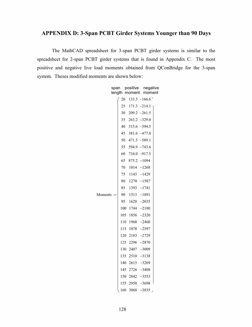
128
APPENDIX D: 3-Span PCBT Girder Systems Younger than 90 Days
The MathCAD spreadsheet for 3-span PCBT girder systems is similar to the
spreadsheet for 2-span PCBT girder systems that is found in Appendix C. The most
positive and negative live load moments obtained from QConBridge for the 3-span
system. Theses modified moments are shown below:
span positive negative length moment moment
Moments
20
25
30
35
40
45
50
55
60
65
70
75
80
85
90
95
100
105
110
115
120
125
130
135
140
145
150
155
160
133.3
171.3
209.2
263.2
315.6
381.6
471.3
594.9
734.0
875.2
1014
1143
1270
1393
1513
1628
1744
1856
1968
1078
2183
2296
2407
2510
2615
2726
2842
2958
3068
166.6−
214.1−
261.5−
329.0−
394.5−
477.0−
589.1−
743.6−
917.5−
1094−
1268−
1429−
1587−
1741−
1891−
2035−
2180−
2320−
2460−
2597−
2729−
2870−
3009−
3138−
3269−
3408−
3553−
3698−
3835−
:=

129
All of the other terms in Appendix C are the same for the 3-span system, except
for the differences that are noted below:
Definition of changed term 2-Span System 3-Span System
Mid-span moment due to deck and
haunch weight M = 8
2lw ⋅ M =
10
2lw ⋅
Moment from permanent composite
dead load at mid-span 0625.02 ⋅⋅= lwM 075.02 ⋅⋅= lwM
Composite dead load restraint
moment l
IEM
⋅⋅⋅=
3θ 83.0
3⋅
⋅⋅⋅=
l
IEM
θ
Prestress restraint moment
l
IEM
⋅⋅⋅=
3θ 83.0
3⋅
⋅⋅⋅=
l
IEM
θ
Differential shrinkage restraint
moment
1.5 * Mdiffsh 1.2 * Mdiffsh
Thermal restraint moment 1.5 * Mthermal 1.2 * Mthermal
Superimposed permanent dead load
moment at mid-span M = 8
2lw ⋅ M =
10
2lw ⋅

130
APPENDIX E: PCBT Details and Section Properties

131
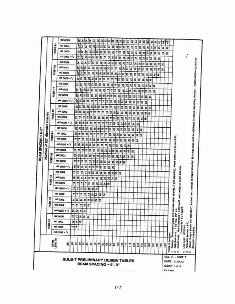
132

133
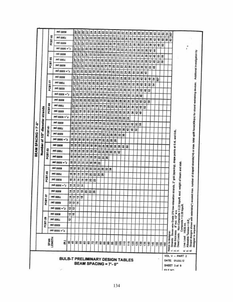
134

135

136
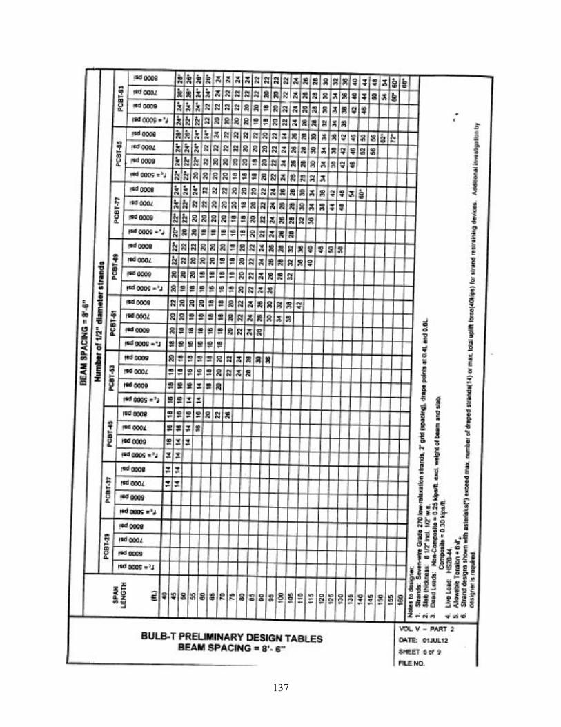
137
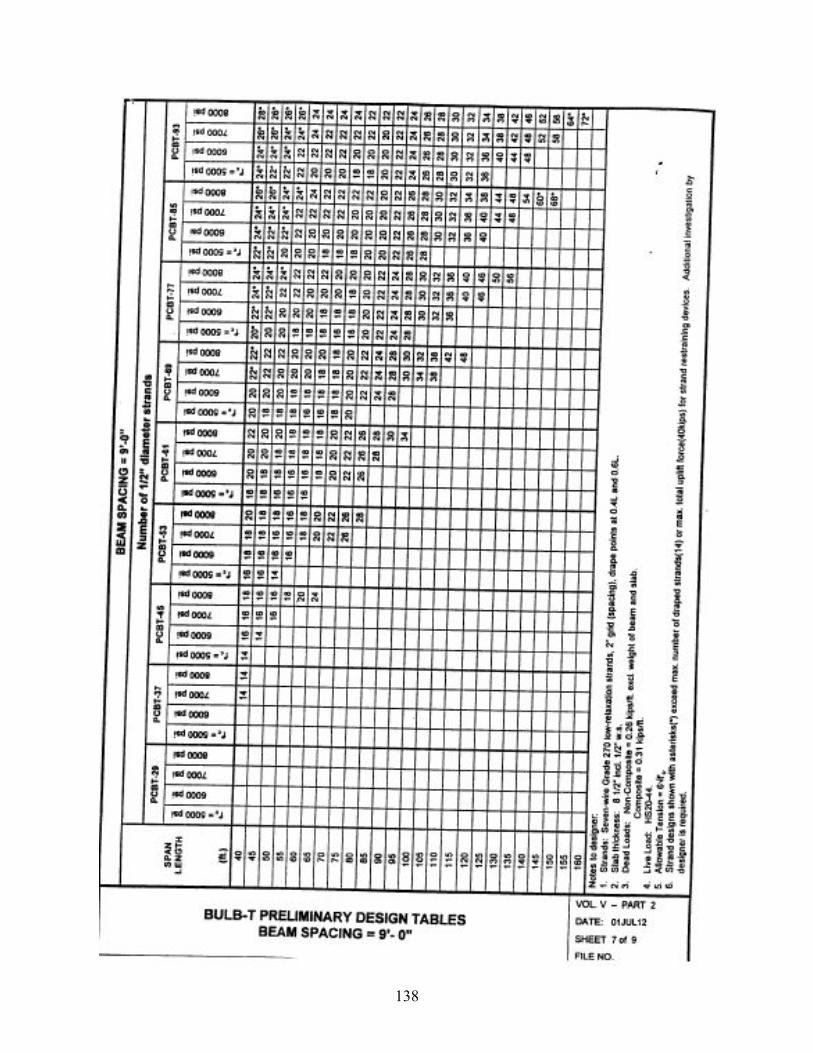
138

139
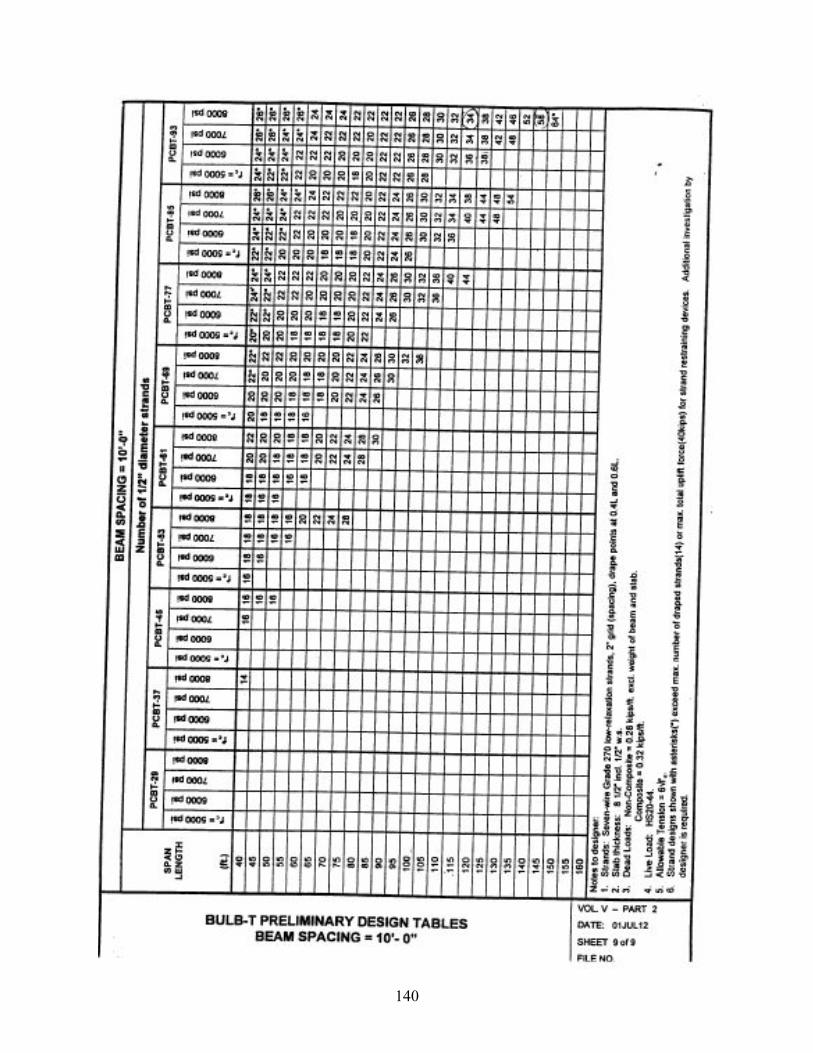
140