Prestige Matters: Value of Connections Formed in Elite Colleges ∗

Sheetal Sekhri†

March 21, 2014

Abstract

This paper provides evidence that graduates of elite public institutions in In-

dia have an earnings advantage in the labor-market even though attending these

colleges has no discernible effect on learning outcomes. Data do not bear out the

predictions of signaling theories of human capital. Using original survey data, I

find that college networks do not facilitate job search. Also, the wage-premium

does not dissipate with experience. However, the number of college friends in the

same industry does explain the wage premium. These results support the hypoth-

esis that the labor market rewards the connections students’ form at elite colleges.

JEL Classifications: I23, J24, O15

∗Funding from International Growth Centre, India Country Team (CPP-IND-CEN-2010-008) isgreatly acknowledged. Zhou Zhang and Sisir Debnath provided excellent research assistance. Thispaper has benefitted from discussions with Ken Chay, Andrew Foster, Leora Friedberg, Claudia Goldin,Kevin Lang, John Pepper, Sarah Turner, Miguel Urquiola, and from suggestions of seminar participantsat Boston University and IGC Growth Week.

†Corresponding author: University of Virginia, PO Box 400182, Department of Economics, MonroeHall, Charlottesville,VA 22904-4182, USA, Email: SSekhri@virginia.edu, Phone:434-982-4286,Fax:434-982-2904

1 Introduction

The reputation of elite institutions attracts the very best students, and the graduates of

such institutions often earn a premium in the labor market. Because college quality af-

fects students’ enrollment decisions and governments’ investment decisions, determining

the returns to quality of higher education is important. Limited credit markets, uncer-

tain labor market conditions, and acute information asymmetries in developing countries

make the need to understand the returns to college quality even more compelling. In

addition to understanding the returns to attending elite institutions from a public fi-

nance perspective, understanding what mechanisms are responsible for generating these

returns- if such return truly exists- is crucial. An understanding of these mechanisms

would enable us to inform policy choices in improving college education and making it

more accessible.

As noted in previous research addressing this question, estimating the returns to

college quality is empirically challenging. The unobserved individual traits that influence

admissions decision, may also affect labor market outcomes. Employing a variety of

methods, previous research focusing on estimating the returns to selective colleges has

found mixed evidence (Dale and Krueger 2002; Black and Smith 2004; Hoekstra 2009;

Saavendra 2009; Dale and Krueger 2011). But minimal evidence is available concerning

the mechanisms by which prestigious institutions may affect labor market outcomes.

One main difficulty in assessing these mechanisms is the lack of comprehensive data that

link school outcomes, college outcomes, family background, earnings, networks, referrals,

and occupation for individuals. Using data from India, this study applies a regression

discontinuity design to estimate the returns to college quality. More notably, it research

employs an original survey to shed light on the black box of the underlying mechanisms.

Attending an elite college can influence an individual’s labor market outcomes in

a number of ways. First, the elite institutions may increase the productivity of the

students as a result of high value added (human capital theory). Second, because such

colleges tend to be more selective, students may also attend prestigious institutions

to signal their ability to prospective employers and distinguish themselves from other

1

prospective employees. The firms may screen applicants on the basis of the type of college

attended, and statistically discriminate in favor of such colleges (signalling theory). A

third possibility is that college graduates develop helpful social networks (networking

theory). This effect can operate in two ways. The networks can help graduates get

better paying jobs by reducing information asymmetries. Additionally, the students’

peers and friends from college are likely to be placed well, and such connections may

matter to employers. Original data, collected via an in-person survey, allow me to isolate

the underlying mechanism.

This paper contributes to the literature in three ways. First, it provides causal

estimates for returns to attending prestigious colleges in India, using the features of

India’s education system. Second, it addresses the mechanisms that can drive the re-

turns. Third, it compiles a comprehensive data set that includes observational data and

in-person interview-based survey data, to test what drives the returns to attending pres-

tigious colleges. Public colleges in India are very prestigious and therefore attract the

best students. Numerous media reports and popular press stories indicate these grad-

uates receive high wages. Average comparisons of common college exit test scores also

show these students out-perform their private counterparts. The admission procedure

to public colleges makes this setting ideal for examining the returns to attending such

colleges. Public colleges admit students based on a cutoff point of the students’ scores

on the Senior Secondary School Examinations.1 I use a unique data set that I collected

to test whether public college graduates earn more than private college graduates. In

doing so, I test whether evidence supports the predictions of the signalling, networking,

or human capital models of higher education. I find that the educational outcomes of

public college students who were on the margin of the admission cutoff do not differ

from those of students who barely missed the cutoff and thus attended private colleges.2

However, graduating from a public college provides a premium in the labor market. I

employ a regression discontinuity design and show the results are robust to several spec-1Senior Secondary School Examinations are the equivalent of high school exit tests in US. Technical

education colleges such as medicine and engineering use different centralized tests for admission.2Rubinstein and Sekhri (2011) use this rule and show the students who barely get admitted to public

colleges perform similarly in college exit tests to those who barely miss and attend private colleges.

2

ifications and methods of estimation. I show that selection into the sample or into being

employed are not likely to bias the results. I do not observe the wages of all employed

individuals in the data, and I cannot rule out selection in reporting wages. However, I

estimate treatment-effect bounds (Lee’s bounds (2009)), which confirm the results.

My findings do not provide evidence for the human capital theory. The average qual-

ity of the college cohort drives the public main effect, implying the selectivity of the

college the employee attended is important to the firms. A first-order prediction of the

signalling model would be that if the public college is a signal, then we should see a

positive return to attending a public college in equilibrium even though public college

attendance does not influence human-capital production. The data support this predic-

tion. However, dynamic learning by firms, as in the framework of Farber and Gibbons

(1996)and Altonji and Pierret (2001), would predict this positive return would diminish

with experience and inframarginal students’ wages would increase with experience. In

addition, the divergence in wages would increase overall but decrease at the admission

threshold. However, the public college returns do not diminish with experience over the

10 year period in the data. The overall wage dispersion does not increase and wages do

not converge around the admission cutoff with experience. Hence, the predictions of the

dynamic learning models are empirically rejected in this setting.

The average quality of the cohort should not affect job referrals. In addition, using

data from several questions asked in the survey, I find no evidence that referrals or job-

search facilitation by networks result in better-paying jobs.3 Besides being consistent

with the signalling model, the average quality of the cohort would also matter if the

firms placed a value on the prospective employee’s connections. The findings weigh

in favor of this model. The number of college friends that public college graduates

have accounts for the majority of the premium. In developing countries such as India,

corruption is rampant and red tape increases the cost of doing business. Thus employers

reward connections and favors that employees’ can bring to the firm. I bolster these

findings with an instrumental variable approach using the eligibility for public colleges

as an instrument for college friends in the same industry.3 See Munshi 2003 for an example in which network ties facilitate job search.

3

Educational networks have been shown to be an important source of information

in the finance industry in the developed world. Cohen, Frazzini, and Malloy (2008)

show that mutual fund managers have vital informational benefits when investing in

firms managed by peers in their education networks. Social ties also matter for busi-

ness decisions. Hong, Kubik, and Stein (2004) show that peers influence stock market

participation. Kelly (2012) shows that educational peers can have a significant effect

on executive decisions about the firms and that these decisions are much more influ-

enced when peers have interacted. In the developing countries context, Khawaja and

Mian (2005) show the values of political connections for businesses by demonstrating

that banks favor politically connected firms in their lending decisions. My paper also

contributes to this literature and presents evidence that firms favor employees with more

connections and ability to network with these connections.

The remainder of the paper is organized as follows: Section 2 provides background

information about general education college education and admission rules. Section 3

discusses the data. Section 4 presents the estimation strategy. Section 5 documents

the results and the findings of robustness tests. Section 6 discusses the mechanisms. I

discuss selection issues in detail in section 7. Section 8 provides concluding remarks.

2 Background

2.1 Public versus Private Colleges

In India, general eduction colleges operate in all districts with the goal of making ter-

tiary education accessible. The colleges account for about nine-tenths of undergraduate

enrollments (Agarwal, 2006), but these colleges are not allowed to confer a degree and

must affiliate with a university to operate. 4 Each college has its own campus and in-

frastructure. Private colleges are managed privately. However, they may receive public

funds (“private aided college”) or they may be totally self-financed (“private unaided4The University Grant Commission Act (UGC), which is the government body that regulates tertiary

education, has a provision that prohibits any institution from awarding degrees unless it is establishedunder an act of Parliament or is specially empowered to award degrees.

4

college”). The private aided colleges can raise funds by charging higher fees and accept-

ing donations from philanthropic or business groups. On the other hand, public colleges

are managed and financed by the government. Public colleges cannot accept any private

donations, and the state funds their maintenance and development expenses. In the sam-

ple, the private aided colleges receive public funds to meet their recurring expenditures

(mostly teacher salaries) and charge much higher tuition than the government colleges.

Although the teachers have to take the same University Grants Commission Exam to

qualify for teaching positions in private colleges, they do not enjoy the same degree of

job security as the government teachers. Their contracts differ from college to college

and are negotiated with the private management. Private colleges also hire more adjunct

teachers on short-term contracts than public colleges. In contrast, public colleges are

managed and run by state employees. Teacher contracts are negotiated with the govern-

ment and offer tenure security. The state funds public colleges’ facilities and equipment,

but private colleges (both aided and un-aided) have to self-finance such expenditures.

Private aided colleges can apply government aid only to pay teachers salaries. Public

colleges are considered very prestigious and students favor these over private colleges.5

2.2 Public College Admissions

Admission to general education public colleges (excluding technical education such as

medicine or engineering etc) is determined on the basis of the students’ performance

on the Senior Secondary School examinations taken in class XII.6 Students cannot be

admitted to college without at least passing this exam, but to be admitted to public

colleges, their score must exceed a specified cutoff. This admission cutoff for public

colleges is determined every year and varies by college and stream of education. Students

who score above the cutoff are eligible for admission to public colleges. Although the

colleges post a list of of students who are offered admission to public colleges, the public5 For example-Presidency college in Calcutta, West Bengal has been an elite public college. It was

converted into a university recently.6Class XII is equivalent to a high school grade 12, the last year of high school. All high schools

in India must be affiliated either with one of the two national boards (Central Board of SecondaryEducation or Indian Certificate of Secondary Education) or with their state’s regional board. The exitexams are conducted by school boards across India and are recognized nationally.

5

does not know the admission cutoffs and rules used to determine the cutoffs are kept

confidential. Students apply to various colleges simultaneously as the admissions open

in the spring. The admission decisions are made public in early fall, shortly before the

start of the academic year. Colleges diligently follow admission rules. The percentage of

students attending public colleges rises sharply from near 0 to above 90 percent around

the admission threshold. Streams are declared in the penultimate year of the high school

2 years before the Senior Secondary School Examinations are taken. Hence, performance

in the exit exams does not affect stream choice.

2.3 Uniform College Exit Tests

All students in colleges (private or public) affiliated with the same university, take the

same exit exams. These exams vary by stream of education, but conditional on the

stream, private and public college students study the same curriculum and take the

same exit tests. These exams test for language competencies( English and regional

language) and stream-specific competencies; for example, commerce students take tests

in accounting, taxation, and so forth. The examinations for the affiliated colleges are

conducted by the respective universities, which also set the course curriculum. The

affiliated colleges only offer prescribed courses. Thus, conditional on the university and

stream, I can compare the educational outcomes of students in public and private colleges

because they take the same exit tests.

3 Data

The data used in the analysis are collected from several different sources. I obtained

admissions records for public and private colleges from a district in North India. These

records include the Senior Secondary School Examination scores, age, gender, place of

residence, board of secondary education, stream of study, and father’s occupation. The

college exit test scores were obtained from the affiliating university. I matched these

admission records and college exit test scores using a unique roll number assigned to

each student. Institutional details on admission cutoffs were obtained from the colleges.

6

The sample included admission cohorts from 1999 to 2002. I conducted a detailed follow-

up survey of these students in 2011-12. 7 I did not survey graduates from rural areas due

to cost considerations in the follow-up survey. Of the 1981 individuals that the survey

tried to locate, 1,506 students (76 percent) were successfully surveyed.

The general education colleges do not offer professional degrees like law or medicine.

In general migration out of district for higher education is low. Students do not migrate

out of their district to attend general education colleges (Rubinstein and Sekhri, 2011).

Private colleges offer merit scholarships which ensures that students around the cutoff

who apply to college attend either public or private colleges. As a further test, I collected

the applications of students who applied but did not get into the public colleges. I verified

that these students had indeed attended colleges. Rubinstein and Sekhri (2011) also

document that the drop-out rate from private and public colleges in India is similar and

the observable characteristics of the students are no different. Neither Senior Secondary

School Examination scores nor father’s occupation influence drop-out decisions very close

to the cutoff; hence students with different abilities and socio-economic backgrounds are

equally likely to drop out on either side of the cutoff.

Besides the administrative data, I also conducted an in-person interview-based survey

that asked detailed questions about labor-market participation. I obtained data on

employment history, duration of each employment, occupation, type of organization

worked for,type of industry, and salary per month. Salary information was elicited as a

categorical variable. The categories included rupees 5,000 or less, 5,000-10,000, 10,000-

15,000, 15,000-20,000, 20,000-30,000, and greater than 30,000. The survey also collected

data on networks and job referrals. The respondents were asked if they were referred to

the job by friends, their spouse’s friends, people who attended their college, people who

attended their spouse’s college, and the number of college friends in the same organization

and industry. Demographic information such as marital status and number of children

were also ascertained.

Of the 1,506 respondents, 748 individuals are either self-employed or earn a salary.7This sample excludes the students admitted to public colleges based on reservation quotas for lower

castes.

7

Those who are either self-employed or earn a salary are considered employed for the

purpose of the analysis. Other possible choices include being a student, being unemployed

and looking for work, being unemployed and not looking for work, home production, and

other. In the sample of successfully located respondents, 40 percent are home makers,

and 99.04 of these individuals are women. Among the formally non-employed, 79 percent

are engaged in home production. Among the employed, 458 out of 748 individuals report

their salary and 439 observations have non missing data for background characteristics.

Selection bias can result from selection into the sample, selection into employment,

and selection into reporting the salary. The implications of selection issues for the results

and robustness tests performed to address these issues are discussed in detail in Section

7. The main sample of analysis comprises individuals who are either self-employed or

earn a salary and have reported their salaries. Table 1 provides the summary statis-

tics. Table 2 provides summary statistics by college type. Appendix Table 1 provides

summary statistics in the -5 to +5 interval of the Senior Secondary School Exam scores

around the admission cutoffs. This table shows the individuals are similar on observ-

able characteristics in narrow intervals around the cutoff in the main sample used in the

analysis.

4 Estimation Strategy

4.1 Empirical Specification

I employ a regression discontinuity (RD) design to estimate the effect of attending public

colleges on wages. Since admission to public colleges is based on a deterministic rule

of Senior Secondary School Exams, I am able to compare outcomes across students

with similar expected productivity(or ability) who are on the margin of the admission

cutoff and hence attend public or private colleges due to small differences in their Senior

Secondary School Examination scores. The application lends itself to a sharp design and

the empirical model is as follows:

8

Yi = αXi + β Publici + f(Si) + ei (1)

where Yi is the outcome variable including salary and college exit test scores. Xi is a

vector of individual characteristics including own demographics and family characteris-

tics. Publici is an indicator variable that takes the value of 1 if the individual attends a

public college and 0 otherwise. β is the parameter of interest and it indicates the effect

of attending public colleges on the outcomes. f(Si) is a function of the Senior Secondary

School Exam scores Si. Robust standard errors are reported. I also show results from

an ordered-logit empirical specification for salary brackets, because salary is recorded as

a ordered categorical variable. I calculate the average marginal effect of public colleges

on being in each salary bracket.

4.2 Sensitivity Analysis

I use both parametric and non-parametric functions of Si to explore the robustness of the

findings to functional-form assumptions. For the parametric specifications, I use linear,

quadratic, and cubic control functions. For the non-parametric specifications, I follow

Hahn, Todd, and van der Klaauw (2001) and use local linear regressions to estimate the

left and right limits of the discontinuity, where the difference between the two is the

estimated treatment effect. Bandwidth choice can also influence results and no widely

accepted guidelines exist for choice of bandwidth. Therefore, for non-parametric analysis,

I vary the bandwidth and show results for several choices. I also show results for the

optimal bandwidth proposed by Imbens and Kalyanarman (2014). Finally, I use both

triangular and rectangular kernels to show the results are not sensitive to the choice of

the kernel.

9

5 Results

5.1 Main Results - Salary and College Exit Test Scores

Public colleges indeed follow admission rules. Figure 1 plots the percentage of students

who attended public colleges in two percentage bins of normalized Senior Secondary

School Exam scores. The top panel shows a polynomial fit and the bottom panel shows

a linear fit. This figure clearly demonstrates that there is a sharp rise in the percentage of

students who attended public colleges around the cutoff. The percentage rises from near

0 to around 90 percent. Figure 2 plots the regression functions from the local polynomial

regression of the salary index on normalized Senior Secondary School scores. Salary is a

categorical variable corresponding to different slabs. The highest value it takes is 6. The

first panel uses a bandwidth of 1.5 and the bottom panel uses the optimal bandwidth as

proposed by Imbens and Kalyanaraman (2014). Appendix Figure 1(a) shows confidence

intervals around the regression function and Appendix Figure 1(b) shows the scatter

plot of the average salary in 2 percentage point bins of the normalized Senior Secondary

School Examination scores in addition to the regression functions. These figures show

that salary exhibits a jump at the admission cutoff for public colleges.

The results depicted in these two figures are formalized, and Tables 3 to 7 report the

estimation results. Table 3 shows the results of an ordinary least squares regression of

salary on the public college indicator. Column (i) reports the coefficient from a simple re-

gression. Pre-college demographic controls including gender, year of admission to college,

age at entering college, stream of study, board of education for Senior Secondary school,

and father’s occupation are added in column (ii). Column (iii) additionally controls for

Senior Secondary School Exam scores. Across these specifications, the coefficient on

public college is positive and highly statistically significant at the 1 percent significance

level. Column (iv) controls for college exit test scores to show the results are robust

to including the college exit test scores. The public college effect corresponds to a 1

category shift in salary, which is large. Table 4 shows the results from the parametric

regression discontinuity analysis. Each cell reports the public college coefficient from a

separate regression. Column (i) reports results from the full sample. Column (ii) re-

10

stricts the sample to 15 percentage points of the normalized Senior Secondary School

Examination scores around the admission cutoff. Column (iii) restricts the sample to a

10 percentage- point interval, and column (iv) to a 5 percentage- point interval. The first

row uses a linear control function of the Senior Secondary School Scores. The second row

uses a quadratic and the third row uses a cubic. All regressions control for pre-college

demographic characteristics mentioned previously. The results are remarkably similar

across all these specifications and statistically significant at the 1 percent level.

In Table 5, I report the results from a non-parametric regression analysis. Each cell

reports the public college coefficient from a separate local linear regression. Panel A

shows the results for a triangle kernel, and Panel B shows the results from a rectangular

kernel. In the absence of clear rules regarding what bandwidth to use, I show the

results for a range of bandwidths. Column (i) uses a bandwidth of 10, column (ii)

uses 7.5, column (iii) uses 5, and column (iv) uses the optimal bandwidth proposed by

Imbens and Kalyanamraman (2014) (IK). In each panel, the first row shows the results

without controlling for any other characteristics and the second row shows the results

with the pre-college demographic controls. These results show a positive and statistically

significant effect of public college attendance on salary. The results are not sensitive to

the choice of the kernel or bandwidth.

Salary is a categorical variable. The index corresponds to six salary slabs. In Ap-

pendix Table 2, I report the ordered logit estimates of the impact of public college

attendance on the probability of being in a given salary bracket. Each cell reports the

marginal effect for the specific bracket. The first row shows the results without any

controls. The second row shows results with demographic controls. The third row con-

trols for pre-college demographic characteristics and the Senior Secondary School Exam

scores. Public college attendance reduces the probability of being in the first, second,

and third salary brackets, has no effect on being in the fourth bracket, and increases the

probability of being in the fifth and sixth bracket. These effects are highly statistically

significant. In the last row, the probability of being in the lowest bracket reduces by 4.2

percent and the probability of being in the highest bracket goes up 17 percent. These

coefficients are large in magnitude.

11

The full sample IV estimate, where I instrument public college attendance with eligi-

bility to attend ( Senior Secondary School Examination Scores > the admission cutoff),

is 1.43 with a standard error of 0.25. As with other approaches, this estimate is highly

statistically significant at 1 percent significance level indicating that public colleges grad-

uates receive a wage premium in labor markets.

5.2 Robustness Checks

The admission rules used to determine the cutoffs are only known internally and the

tests are evaluated externally using a double-blind method. Hence, little scope exists

for manipulation of Senior Secondary School Exam scores. I present evidence from the

McCrary density test to highlight that the students do not manipulate their Senior Sec-

ondary School test scores. The results are shown in Appendix Figure 2. The distribution

of the Normalized Senior Secondary School Exam scores on the left and right of the dis-

continuity are similar and exhibit no jump around the cutoff.

Another possible concern might be that the background characteristics of the indi-

viduals vary around the cutoff. This concern can lead to the spurious attribution of

treatment effects to treatment when the results are caused by these other variables that

exhibit a jump near the discontinuity. Appendix Table 1 shows that the control variables

including demographic characteristics and family background are similar in the -5 to +5

interval of Senior Secondary School Exams scores around the public college admission

cutoff. I also show that these variables are smooth around the cutoff graphically in

Appendix Figure 3.

6 Mechanisms

The results shown so far establish that the labor-market rewards attending public col-

lege. Wages are higher for the public college graduates than for their private college

counterparts. Four possible alternative mechanisms can explain these results.

First, the students may learn more in public colleges and this learning increases their

productivity. Not only the teachers, but peers as well can contribute to such learning.

12

Second, the employers may use public colleges as a signal of quality as in the classical

signalling hypothesis put forward by Spence (1973) and Weiss (1995). In equilibrium,

this hypothesis will translate into higher wages for public college graduates, but the

college would not contribute to the students’ human capital. Suppose the employers

form a prior that the average quality of students entering the public colleges is better

than those entering private colleges. Then they would statistically discriminate in the

favor of public college graduates without knowing the true quality of the marginally

admitted student.8

The third hypothesis is that the public college graduates have a wide network of

alumni who help them get better jobs, which pay higher wages. A large literature in

labor shows that networks help individuals find jobs by reducing information asymmetry.9

Thus, the college network may provide referrals for the students, and public college

students have better access to such networks. The fourth explanation might be that the

labor market rewards the potential connections that the students might have made in the

college. If public college students are expected to be in important positions in government

or the private sector, a firm may value a student who knows these key personnel. This is

more relevant in a developing country such as India where connections can be vital for

doing business.10I test these alternate hypothesis to discern why is there a labor market

premium on attending public colleges.8Note that a number of reasons can account for the absence of value added by the public colleges.

MacLeod and Urquiola (2009) propose that students who enter prestigious institutions may not exerta high degree of effort while in college. Thus, marginally admitted students will perform just like theirprivate counterparts on college exams, but the labor market will still favor the reputation of the college.If elite institutions are selective, students ought to experience positive peer effects as proposed by Eppleand Romano (1998). Public college employees have a high degree of job security in India. They mightnot invest in teaching. So, teachers’ lack of effort cancels out the gains from the peer effects. A work-in-progress paper addresses these mechanisms. For this study, in both these cases, public colleges can serveas a signal even if they do not contribute to the human capital of the marginally admitted student. Thefocus of this paper is on isolating what drives the returns to attending public colleges in labor markets,and not on shedding light on the production function of the colleges.

9Montgomery (1991) provides a review of this literature. Munshi (2003) shows that network referralsmatter for job placement.

10Khwaja and Mian (2005) provide insights about financial benefits of political connections for firmsin Pakistan.

13

6.1 Human Capital

So far, the results have shown a large robust effect of attending public colleges on salary

earned post college. If the human capital theory of education is driving these results,

we should observe a positive and large effect on college examinations as well. Note as

explained 2.3, students of the left and right of the admission cutoff take identical college

exit exams even though they attend different types of colleges. I test if the college

exit test scores of the marginal students in public colleges are higher than the private

counter-part for this sample and report the results in Table 6. I show the results from a

parametric regression discontinuity design analysis. 11 Each cell again reports the results

from a separate standardized regression. As before, column (i) reports results from the

full sample. Column (ii) restricts the sample to 15 percentage points of the normalized

Senior Secondary School Scores around the admission cutoff. Column (iii) restricts the

sample to a 10 percentage point interval, and column (iv) to a 5 percentage point interval.

The first row uses a linear control function of the Senior Secondary School Scores. The

second row uses a quadratic and the third row uses a cubic. All regressions control for pre-

college demographic characteristics. Since I show the standardized coefficients, I report

the t-statistics in the brackets. This sample also bears out the findings of Rubinstein and

Sekhri (2011). We do not see an effect of public college attendance on college exit test

scores. None of the coefficients is significant at conventional significance levels.12 The

full sample instrumental variable estimate where public college is instrumented with

eligibility is -0.03 with a t statistic of -0.32. 13

11Non-parametric results are similar and have not been shown in the interest of brevity.12One concern might be that the college exit tests do not capture differences in learning. Students

just memorize the material by rote learning, expecting what the exam will ask, and thus the college exitexam scores are no different in public versus private colleges. In the survey, the students were asked ifthey learned anything in college. Appendix Figure 4 shows that self-assessment of learning in college ispositive and increases with the Senior Secondary School Exam Scores.

13 A growing number of studies in both developed and developing countries examine whether attendingelite schools in K-12 setting improve test scores and find mixed evidence. See Mbiti and Lucas (2013)for a survey of these studies. In the context of a developing country, Mbiti and Lucas (2013) examinethe impact of elite high schools in Kenya and find that elite schools do not result in better academicoutcomes. Saavendra(2009) examines return to elite university education in Columbia and finds thatdifferential college inputs lead to better academic outcomes.

14

6.2 Selectivity of Colleges

I first show that college selectivity as measured by the average quality of the cohort

with whom you enter college (as defined by your college, stream of study, and year

of admission) drives the public college effect on salary. Appendix Table 3 shows the

results of the parametric regression discontinuity analysis. Each cell is the public college

coefficient from a separate regression and the standard errors are clustered at the college-

stream level. The specifications are similar to those in Table 4. I use the full sample,

15, 10 and 5 percentage point intervals of Senior Secondary School Exam scores around

the cutoff, and three specifications for the control function- linear, quadratic, and cubic.

For the sake of comparison, the first row in each panel repeats the results reported in

Table 4 for comparison. The second row reports the coefficient on public college after

controlling for the average Senior Secondary School Examination scores of your cohort.

In comparing the first and second rows in each panel, we see the average quality of the

cohort explains the public college effect. The coefficient changes from large and positive

to small and statistically indistinguishable from 0. This result can be consistent with

the signalling hypothesis or the connections valued by firms. But the average quality of

the cohort should not matter for networks mediating referrals.

6.3 Other Applied Skills Acquired in College

The public colleges may provide inputs that result in better applied skills that the labor

market rewards. According to a recent survey of employers’ perspectives on the corporate

workforce in United States, the top applied soft skills that the firms wanted in their

employees were critical thinking, communication, team work, and collaboration, and

professionalism.14 Although we do not directly measure these soft skills, we can infer

whether college students have a better applied skill set by observing their behavior.

Survey questions measure whether the public college students are more informed, use

technology better, have better team and leadership skills, and are more confident and less14In collaboration, The Conference Board, Corporate Voices for Working Families, the Partnership

for 21st Century Skills, and the Society for Human Resource Management conducted an in-depth studyof the corporate perspective on the readiness of new entrants into the U.S. workforce. This report isbased on the surveys conducted.

15

disruptive. I also examine whether they have higher a propensity to network. Table 7

shows the results from a parametric analysis in the -5 to 5 interval around the admission

cutoff. No difference exists between (i) reading the newspaper, (ii) using the internet, (iii)

helping non-friends with college work, (iv) lending notes to non-friends,15 (v) winning

awards in college, and (vi) being punished in college. However, the public college students

do seem to have a higher propensity to network. The public college graduates spent more

time with peers in their stream (college major). The coefficient is marginally significant

at 10 percent. They also spent more time with people outside their stream and this

coefficient is even larger than the one on ‘own stream students’. They also report having

more friends in college. This is indicative of the fact that public college students do

acquire skills to network better. I also use the false discovery rate procedure proposed

by Benjamini and Hochberg (1995) to test for the joint significance of the nine outcomes.

Only hours spent with students out of stream is significant at 5 percent.16 Thus, the

public college students do tend to network with their out of stream peers.

6.4 Training, Occupation, and Sector

Public colleges can affect labor market outcomes by affecting choice of occupation, sector,

and any other training. I use the survey questions and examine whether public college

attendance affects if the students (i)acquire a diploma (training certificate) , (ii) earn a

post graduate degree, (iii) enter professional specialization , or (iv) study or work abroad.

I also examine whether the students who attend public college are more likely to be in

rewarding jobs such as tertiary-sector jobs or skilled occupations. I test whether they are

employed in public enterprizes and whether they have a higher job turn-over. Table 8

reports the results from a parametric analysis in a -5 to +5 window around the admission

cutoff. None of these factors are statistically different from 0. These attributes do look

fairly comparable across the private and public college graduates near the admission15Almost everyone reports helping friends and lending them notes. I cannot examine the differential

effect on helping friends due to lack of variation.16The p-values used for the individual hypothesis for the false discovery rate are reported in the table.

16

cutoff.17 Using the Benjamini and Hochberg (1995) false discovery rate procedure for

testing the significance of these 8 outcomes, I find that all of these are jointly statistically

insignificant at 5 percent level significance level.

6.5 Signalling- Dynamic Learning

Farber and Gibbons (1996) and Altonji and Pierret (2001) frameworks of dynamic learn-

ing by employers in a signalling framework implies that as employers learn more about

the ability of the employee, the public college effect should diminish with experience.

I conduct three tests to examine whether signalling is important. First, the employers

would initially pay an average salary for the college cohort. But as the employers learn

over time about the employees’ ability, the dispersion in the unconditional salary should

increase. The salary conditional on Senior Secondary School Exam Scores should con-

verge. In other words, salary should converge near the admission cutoff with experience.

Appendix Figure 5 shows the distribution of salary for 0-6 years of experience. In panel

A, the dispersion of the unconditional salary does not increase with years of experience.

The coefficient of variation is 35.3. In panel B, we do not see any evidence of convergence.

The coefficient of variation is still 33.85.

In the second test, I determine whether higher Senior Secondary School Examination

scores, which are a proxy for ability, are rewarded more over time. More formally, I test

whether λ is positive or zero in the following extension of equation 1:

Yi = αXi+β Publici+γ Experiencei+δ Public ∗Experiencei+λ Si ∗Experiencei+f(Si)+ei

(2)

λ > 0 would imply that firms learn over time and use college type as a signal. I plot

salary as a function of the Senior Secondary School Examination scores by experience

in Appendix Figure 6. We do not observe a systematic pattern emerging. As graduates

gain more experience, the slope is flat rather than positive. Table 9 reports the results17Some of these features may be measured imprecisely. If anything, however they have a negative

sign and hence cannot explain the positive public college wage premium.

17

of the regression analysis. I use a full sample parametric analysis with a linear control

function. In column (i), we see a public college premium for salary. Experience is

strong and positive and the squared term is small, negative, and statistically significant

(column (ii)). The public college premium is still strong and positive. In column (iii), the

interaction of public college and experience turns out to be statistically indistinguishable

from 0. In column (iv), I interact Senior Secondary School exam scores with experience.

The public college effect is strong and positive. The coefficient on the interaction is

negative but small and not statistically distinguishable from 0.

The third test checks if the public college premium dissipates with time. This test

checks if δ is zero in the RD frame work. If firms learnt over time then δ would drop

to zero with experience. Appendix Figure 7 shows 6 panels plotting the public college

premium at the admission cutoff by years of experience. We see that the premium persist

over years. Hence we do not find conclusive evidence to support the signalling hypothesis

in which dynamic learning occurs over 6-10 years of experience.

6.6 Network Referrals

The results in Appendix Table 3 suggest network referrals are not the main mechanism

driving the results. I test for the network effect more directly using the survey data. I

restrict the sample to the 5 percentage point interval of Senior Secondary School exam

scores and look at the whether public college graduates are more likely to (1) be referred

for a job by a friend, (2) get a job based on a friend’s referral, (3) have more college

alumni at their organization, and (4) receive a recommendation for a job from college

alumni. I also examine if public college attendees are more likely to be referred for a

job by a friend of the spouse, get a job based on a referral by spouse’s friend, have more

of the spouse’s college alumni at the organization, and get a referral by the spouse’s

college alumni. The results are reported in Table 10. None of these factors are positive

and statistically significant. Only one variable - recommended for a job by a friend- is

influenced by the type of college attended, but the coefficient is negative and statistically

significant. Private college graduates are more likely than public college graduates to

receive a job referral from a friend.

18

6.7 Networks- Value of Connections

The survey asked the respondents how many college friends they have in the same in-

dustry in which they work. In order to directly evaluate whether the connections of the

public college employees matter, I add the number of friends that an individual has in

the industry to the specification. I also interact the number of friends with the public

college indicator. Table 11 shows the results from a full sample parametric analysis with

a linear control function. Column (i) shows that salary increases with the number of

friends the individual has from the same college. The coefficient is positive and statisti-

cally significant. In column (ii), I add the interaction of number of friends from college

and public college. The public college coefficient drops by one-third and becomes in-

significant. However, the interaction is positive and significant. I interpret this result as

evidence that the firms value their employees’ connections. Columns (iii) and (iv), show

that this effect is robust to controlling industry fixed effects and is not driven by public

college graduates being channeled into specific industries. 18 In Appendix Table 4, I

show results from an instrumental variable regression in which I instrument the num-

ber of college friends in the industry with the eligibility for public colleges. The wage

premium associated with the college friends in the industry is high and significant. 19

Results from Tables 7 and 11 indicate two facts. Public college students have more

friends in college and spend more time with their peers and the firms favor employees

with more connections and ability to network with these connections. More connections

can put the employees at informational advantage or benefit them due to pure peer

favors.

Alternate Interpretation: An alternate interpretation might be that underlying

selection mechanisms by firms such that they only hire the inframarginal students (who18I do not observe the rank or position of the friends from same college of the surveyed individuals.

Hence I cannot address the important of the degree of influence. Many industries do have intermediatevalue addition, so connections can matter. For example, in textiles, one of the largest employer in thesample, firms deal in yarn manufacturing, dyeing, processing, weaving, garments, and so forth.

19The underlying empirical model is as follows: The structural relation is given by the equation,Wi = α1 +α2 Fi +α3 Xi +ei. This is the second stage. Wi is the salary of individual i, Fi are individuali’s number of college friends in the industry, Xi are the characteristics of the individual. The first stageis given by : Fi = β1 + β2 E

Pi + β3 Xi + ei. Thus the number of friends in the industry is instrumented

by eligibility for public college attendance (E)P .

19

would be smartest in their cohort) from the public colleges in their area of specialization.

These students may be better trained, have a comparative advantage in the industry,

and thus receive a high pay. The marginal students are hired in different industry. This

could potentially generate the positive effects of friends in an industry on salary and wipe

out the public college premium. In order to examine this possibility, I calculate the mean

number of friends in industry in bins whose X axis is the normalized Senior Secondary

School Examination scores and Y axis is the salary. If the explanation posited above

was true, we should see more number of friends reported for inframarginal individuals

who earn more. Appendix Figure 8 shows the plot. The scale represents the 5 quintiles

of the distribution of mean number of friends in the industry. In this figure, the above

hypothesis will translate into higher average number of friends reported in the upper

right quadrant. Two facts emerge from this figure. First, we do see that people who earn

more on the average report having higher number of friends. Second, however this is not

skewed towards inframarginal students. The distribution is evenly balanced. Hence this

selection mechanism is not driving the results.

7 Implications of Selection

As mentioned above, three main data problems may be a concern for selection. First,

since the data are collected via a survey, selection into the sample could occur. However,

the success rate of the survey does not differ among private and public college graduates.

In a -5 to + 5 interval of the public college admission cutoffs, the rate of survey success

is 33.4 percent in private colleges and 32.19 percent in public colleges. These rates are

comparable on the margin of admission as show in Appendix Figure 9. If the sample

selection rates in treatment and control groups are similar and if the monotonicity as-

sumption holds, a comparison of treatment and control means is a valid estimate of the

treatment effect (Lee, 2009).20 I also check whether observable differences are present20Monotonicity will imply attending public colleges cannot affect difficulty to locate respondents in

either direction. That is - it cannot be that some public college graduates are more difficult to traceand some are very easy.

20

between the surveyed and non-surveyed graduates by college type in this window.21 In

Appendix Table 5, I compare the characteristics of the individuals who were successfully

traced and surveyed to those who were not located by college type in a -5 to + 5 interval

of the public college admission cutoffs. None of the characteristics are different except

one. Fewer Science majors who graduated from public colleges were traced. If science

majors earn less than other majors, their under-representation in public college salary

sample can cause an upward bias in the results. This possibility seems unlikely. 22

The second issue is that the salary is reported conditional on being employed. If

public college attendance also affects the likelihood of employment, an increase in em-

ployment can influence salary. I examine whether having attended a public college affects

the probability of the individual being employed. In Appendix Table 6, I show the results

from a parametric regression discontinuity analysis.23Public college attendance does not

affect probability of being employed in any of the specifications. Since probability of be-

ing employed is no different for public versus private college graduates in narrow intervals

around the admission cutoff, the results are not biased by selection into employment. 24

Finally, there could be selection into reporting the salary. Not every employed individ-

ual reported their salary. If salary were missing at random, the results will be unbiased.

Imputing salary information is possible. Appendix Table 7 shows the differences in ob-

servable characteristics of the individuals who report their salaries to the characteristics

of ones who did not.Individuals who report their salaries are marginally younger, took

their Senior Secondary School Examinations from the central board of secondary exams,

are males whose fathers are in business and they graduated from the commerce stream.

If their incomes are higher than average, which is likely, their under-representation in the21Students who were not traced in the survey look comparable to the ones who were successfully

surveyed on important observable dimensions. Notably, their Senior Secondary School Exam Scoresthat sort them into public and private colleges are very similar and statistically indistinguishable. Thefull sample comparison is available from the author.

22In a regression determining the correlates of salary, being in science stream is uncorrelated withsalary conditional on reporting and being employed. Results are available on request.

23Non-parametric RD analysis shows the same results, which are available upon request.24The majority of the non-employed in the sample are women engaged in home production. In a +5

to -5 interval of Senior Secondary School Examination Scores around the admission cutoff, the resultsare robust to the two extreme-case scenarios- all women engaged in home production would have earnedthe highest value for salary and all women in home production would have earned the lowest level ofsalary observed in the data. Results are available upon request.

21

public colleges near the cutoff can generate an upward bias. If, however, their incomes

are lower than average, their under- representation in private colleges can generate an

upward bias. Therefore, we need to examine whether they are under-represented in the

public colleges near the cutoff of admission. In an interval of -5 to +5 percentage points

around the cutoff for admission, 24.8 percent individuals in public colleges do not report

their salary. However, for private colleges, this number is only 10 percent. Appendix

Figure 10 shows that the probability of reporting salary jumps down in public colleges at

the cutoff of admission. This finding suggests the bias is in fact attenuating the results.

I determine Lee’s bounds for the estimated effect. Appendix Table 8 shows the bounds

and the confidence interval for the estimated effect based on Imbens and Manski(2004).

The confidence interval for the effect, [0.44331.9002] is fairly tight and does not contain

0. Lee’s Bounds (lower bound of 0.73 and upper bound of 1.6) are highly statically

significant. Neither confidence interval covers 0. In the labor markets, public colleges do

yield a premium over private colleges.

8 Conclusion

Using a regression discontinuity design to address selection, this research demonstrates

a substantial earnings advantage associated with public college attendance in India,

although we observe no discernible effects of the type of college on learning outcomes.

Three possible theories can explain these findings. The first hypothesis is derived from

the classical signalling model of education. Public colleges in India are prestigious and

admit the best students. Therefore, firms use college type to statistically discriminate.

The signal value of public colleges results in better wages. The second possibility is

that public college graduates have better alumni networks that help reduce information

asymmetry and result in better labor market outcomes. The third explanation is that

public college graduates have a network of friends holding important offices, and such

relations warrant a premium in the labor market because they reduce the cost of doing

business or result in direct or indirect rents to the firms.

The specific findings are that network referrals are not driving the public college

22

premium. Direct survey-based questions indicate network referrals are not responsible

for the better labor market outcomes of public college graduates. The public college

premium does not dissipate with experience, which is inconsistent with the dynamic

learning models of signalling. If signalling were important, then as firms learn more

about the quality of employees, they should rely less on college type as a signal. We do

not however, observe this. We also do not observe firms learning more about ability of the

employees over time. Public college students have a higher propensity to network, and

have a better placed network. The number of college friends in the industry explains

the public college premium, and public college students spend more time developing

friendships with peers. Hence, the findings are consistent with the hypothesis that the

firms value connections and pay a premium in wages for such connections. This premium

in turn ascribes a reputation to the colleges, which might be an important determinant

of the type of college that students attend. From policy perspective, if private colleges

held networking events and internship programs to strengthen ties with businesses, they

will be able to compensate for the lack of prestige in the labor market.

23

References

[1] Agarwal,P. (2006), “Higher Education in India:need for Change”, ICRIER Working

Paper No. 180,

[2] Aghion , P.,L. Boustan,C. Hoxby, and J. Vandenbussche (2005),“Exploiting States

Mistakes to Identify the Causal Impact of Higher Education on Growth” Harvard

University Mimeo

[3] Altonji, J. and C. Pierret(2001) ,“Employer Learning and Statistical Discrimina-

tion”, Quarterly Journal of Economics, Vol. 116(1), pp. 313 - 50

[4] Benjamini, Y., and Y. Hochberg (1995),“ Controlling the False Discovery Rate:

A Practical and Powerful Approach to Multiple Testing”, Journal of the Royal

Statistical Society, Series B, Vol. 57(1),pp. 289 - 300

[5] Cohen, L., A. Frazzini, and C. Malloy(2010), “Sell Side School Ties,” Forthcoming

Journal of Finance

[6] Dale, S. and A.B. Krueger (2002), “Estimating The Payoff To Attending A More

Selective College: An Application Of Selection On Observables And Unobservables”

Quarterly Journal of Economics, 117(4), 1491-1527

[7] Dale, S. and A. Krueger (2011), “Estimating the Return to College Selectivity over

Career Using Administrative Earning Data”, Princeton University Working Paper

No. 563

[8] Department of Higher Education, Government of India, Annual Reports 2003-04,

2006-07.

[9] Epple, D. and R. Romano (1998), “Competition between Private and Public Schools,

Vouchers, and Peer-Group Effects,” American Economic Review, Vol. 88(1), pp 33-

62

24

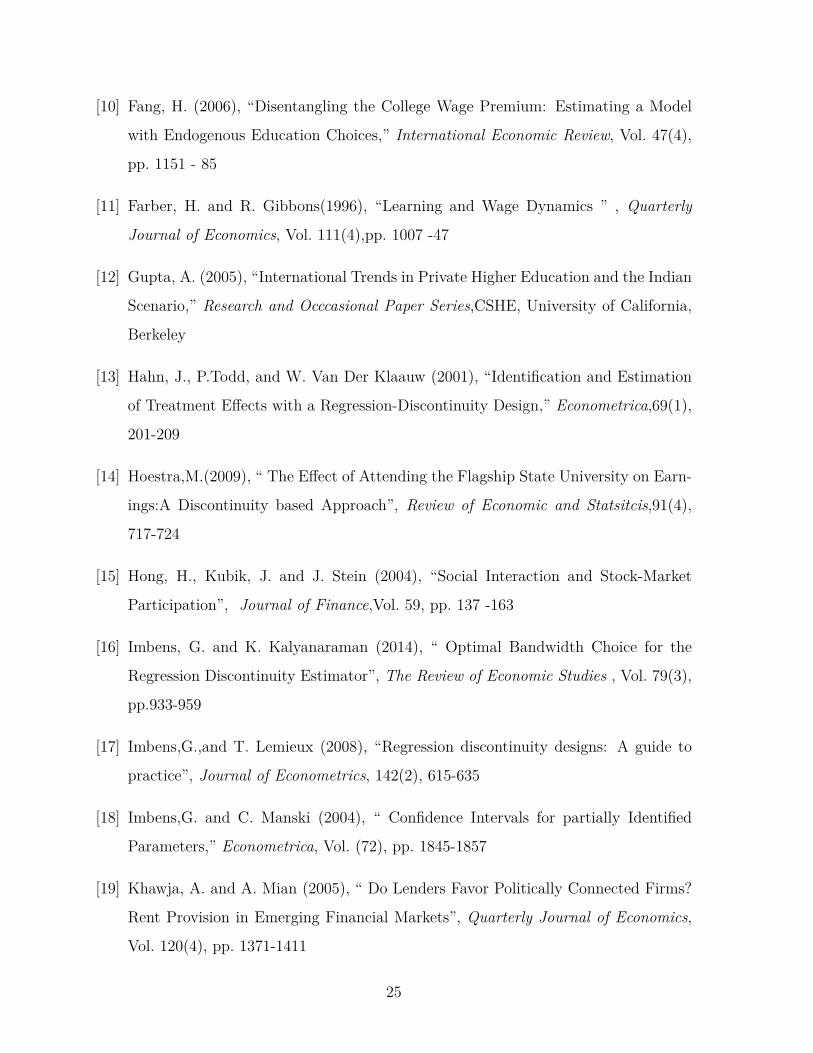
[10] Fang, H. (2006), “Disentangling the College Wage Premium: Estimating a Model

with Endogenous Education Choices,” International Economic Review, Vol. 47(4),

pp. 1151 - 85

[11] Farber, H. and R. Gibbons(1996), “Learning and Wage Dynamics ” , Quarterly

Journal of Economics, Vol. 111(4),pp. 1007 -47

[12] Gupta, A. (2005), “International Trends in Private Higher Education and the Indian

Scenario,” Research and Occcasional Paper Series,CSHE, University of California,

Berkeley

[13] Hahn, J., P.Todd, and W. Van Der Klaauw (2001), “Identification and Estimation

of Treatment Effects with a Regression-Discontinuity Design,” Econometrica,69(1),

201-209

[14] Hoestra,M.(2009), “ The Effect of Attending the Flagship State University on Earn-

ings:A Discontinuity based Approach”, Review of Economic and Statsitcis,91(4),

717-724

[15] Hong, H., Kubik, J. and J. Stein (2004), “Social Interaction and Stock-Market

Participation”, Journal of Finance,Vol. 59, pp. 137 -163

[16] Imbens, G. and K. Kalyanaraman (2014), “ Optimal Bandwidth Choice for the

Regression Discontinuity Estimator”, The Review of Economic Studies , Vol. 79(3),

pp.933-959

[17] Imbens,G.,and T. Lemieux (2008), “Regression discontinuity designs: A guide to

practice”, Journal of Econometrics, 142(2), 615-635

[18] Imbens,G. and C. Manski (2004), “ Confidence Intervals for partially Identified

Parameters,” Econometrica, Vol. (72), pp. 1845-1857

[19] Khawja, A. and A. Mian (2005), “ Do Lenders Favor Politically Connected Firms?

Rent Provision in Emerging Financial Markets”, Quarterly Journal of Economics,

Vol. 120(4), pp. 1371-1411

25

[20] Kingston, P. and L. Lewis editors(1990), The High Status Track: Studies of Elite

Schools and Startification, State University of New York Press

[21] Lang, K. and E. Siniver (2011), “Why is an elite undergraduate education Valuable?

Evidence from Israel”,Labour Economics, Vol. 18, pp. 767-777

[22] Lee, D (2009), “ Training , Wages , and Sample Selection: Estimating Sharp Bounds

on treatment Effcets,” Review of Economic Studies, Vol. (76), pp. 1071-1102

[23] MacLeod, B. and M. Urquiola (2009), “Anti-Lemons: School Reputation and Edu-

cational Quality,” NBER Working Papers 15112

[24] Mbiti, I. and A. Lucas (2013), “Effects of School Quality on Student Achievement:

Discontinuity Evidence from Kenya”, forthcoming(American Economic Journal:

Applied Economics

[25] Munshi, K. (2003), “ Networks in the Modern Economy: Mexican Migrants in the

U.S. Labor Market, ”Quarterly Journal of Economics, Vol. 118(2), pp. 549-599

[26] Montgomery, J. (1991), “ Social Networks and Labor-Market Outcomes: Toward an

Economic Analysis,” American Economic Review, LXXXI, pp. 1408 - 1418

[27] Rubinstein, Y. and S. Sekhri (2011), “Public Private College Educational Gap in

Developing Countries: Evidence on Value Added versus Sorting from General Edu-

cation Sector in India ” Working Paper, University of Virginia

[28] Saavendra, J .(2009), “ The Returns to College Quality: A Regression Discontintuity

Analysis”, Unpublished paper, Harvard University

[29] Shue,K. (2012), “ Executive Networks and Firm Policies: Evidence from the Ran-

dom Assignment of MBA Peers”, unpublished manuscript

[30] Spence, M. (1973), “Job Market Signaling” Quarterly Journal of Economics,Vol.

87(3), pp. 355 -74

[31] UNESCO (1998), “Higher Education in India: Vision and Action”,UNSECO World

Conference on Higher Education in the Twenty-First Century

26

[32] Weiss, A.(1995), “Human Capital vs. Signalling Explanations of Wages ” Journal

of Economic Perspectives, Vol. 9(4), pp. 133 -54

27

 

 

                           Figure 1: Discontinuity in Attending Public Colleges  

 

 

02

04

06

08

01

00

Pe

rcen

tage

in P

ublic

Col

lege

s

-22 -14 -6 2 10

Normalised Senior Secondary School Score Bins

02

04

06

08

01

00

Pe

rcen

tage

in P

ublic

Col

lege

s

-22 -14 -6 2 10

Normalised Senior Secondary School Score Bins

 

                             Figure 2: Discontinuity in Salary at the Public College Admission Cutoff 

23

45

Sa

lary

Bra

cke

ts

-30 -20 -10 0 10 20

Normalized Senior Secondary School Exam Scores

Bandwidth (1.5)

The Impact of Public Colleges on Salary1

23

45

6

Sa

lary

Bra

cket

s

-30 -20 -10 0 10 20

Normalized Senior Secondary School Exam Scores

IK - Optimal bandwidth

The Impact of Public Colleges on Salary

Table 1: Summary Statistics

N Mean  Std. Dev. 

Salary 439 4 1.44

Senior Secondary School Exam Scores 439 66.57 10.09

Central Board of Secondary Education 439 0.25 0.43

Age at Starting College 439 18.03 0.9

Father's Occupation

              Government Service 439 0.08 0.27

              Labor in Unorganized Sector 439 0.07 0.25

              Professional 439 0.05 0.22

              Service in Formal Sector 439 0.32 0.46

               Agriculture 439 0.07 0.26

                Business 439 0.3 0.45

Admission Year

1999 439 0.21 0.41

2000 439 0.3 0.45

2001 439 0.25 0.42

2002 439 0.24 0.43

Male 439 0.4 0.5

Stream

Commerce 439 0.24 0.43

Liberal Arts 439 0.51 0.5

Science 439 0.24 0.42

College Exit Test Scores 439 1255.18 274.93

Public Colleges 439 0.432 0.5

Table 2: Summary Statistics by College Type

Public Private

mean std dev mean std dev Difference

Salary 4.67 1.4 3.5 1.5 1.18***

Senior Secondary School Exam Scores 72.8 7.6 61.8 9 10.9***

Central Board of Secondary Education 0.32 0.46 0.2 0.4 0.12***

Age at Starting College 18 0.88 18.05 0.92 0.05

Father's Occupation

              Government Service 0.09 0.3 0.07 0.26 0.018

              Labor in Unorganized Sector 0.057 0.23 0.08 0.27 0.02

              Professional 0.03 0.18 0.06 0.25 0.03

              Service in Formal Sector 0.38 0.46 0.27 0.44 0.1**

               Agriculture 0.07 0.26 0.07 0.25 0.001

                Business 0.24 0.43 0.32 0.47 0.08*

Admission Year

1999 0.22 0.41 0.21 0.41 0.008

2000 0.34 0.47 0.24 0.43 0.09**

2001 0.22 0.41 0.26 0.44 0.03

2002 0.21 0.4 0.27 0.44 0.06

Male 0.57 0.5 0.266 0.44 0.31***

Stream

Commerce 0.22 0.41 0.26 0.44 0.04

Liberal Arts 0.56 0.5 0.46 0.5 0.1**

Science 0.21 0.4 0.26 0.44 0.05

College Exit Test Scores 1302.8 275.97 1218.83 269 84***

Observations 190 249

Table 3: OLS Estimates of the Effect of Public Colleges on Salary

Dependent Variable: Reported Salary in 6 Categorical Brackets

(i) (ii) (iii) (iv)

Public College 1.18*** 1.08*** 1.05*** 1.07***(0.12) (0.13) (0.19) (0.19)

Demographic Controls No Yes Yes Yes

Senior Secondary School  Exam Scores No No Yes Yes

College Exit Test Scores No No No Yes

Observations  439 439 439 439R‐square 0.16 0.24 0.24 0.26

Notes:Demographic controls include gender, year of admission in college, age at entering college, stream of study, board of education for Senior Secondary school, and father's occupation. Robust standard errorsare reported in parenthesis. Public College is an indicator equal to 1 if the individual attended public college and 0 if the individual graduated from a private college.*** indicates significance at 1 percent level, ** at 5 percent and * at 10 percent

Table 4: Parametric RDD Estimates of the Effect of Public Colleges on Salary

                                      Dependent Variable: Reported Salary in 6 Categorical Brackets

                                                                       Public College Coefficients 

Full sample 15 Point  10 Point  5 Point Interval Interval Interval

 Senior Secondary School Exam Scores (i) (ii) (iii) (iv)

Linear  Control Function 1.05*** 1.02*** 0.95*** 1.2***

(0.19) (0.2) (0.2) (0.24)

Quadratic Control Function 1.08*** 1.04*** 0.96*** 1.18***

(0.2) (0.2) (0.2) (0.23)

Cubic Control Function 1.15*** 1.08*** 0.97*** 1.2***

(0.2) (0.2) (0.22) (0.24)

Observations  439 384 309 167

Notes:Demographic controls include gender, year of admission in college, age at entering college, stream of study, board of education for Senior Secondary school, and father's occupation. Robust standard errorsare reported in parenthesis. Public College is an indicator equal to 1 if the individual attended public college and 0 if the individual graduated from a private college.*** indicates significance at 1 percent level, ** at 5 percent and * at 10 percent

Table 5: Non-Parametric RDD Estimates of the Effect of Public Colleges on Salary

                                      Dependent Variable: Reported Salary in 6 Categorical Brackets

                                                                          Public College Coefficients 

A: Kernel ‐ Triangle Bandwidth=10 Bandwidth=7.5 Bandwidth=5 IK ‐OptimalBandwidth

 Senior Secondary School Exam Scores (i) (ii) (iii) (iv)

Without Controls 2.2*** 2.36*** 2.37*** 2.2**

(0.48) (0.6) (0.8) (0.94)

With Controls 1.86*** 1.92*** 1.47*** 1.32**

(0.43) (0.5) (0.5) (0.55)

B: Kernel ‐ Rectangular Bandwidth=10 Bandwidth=7.5 Bandwidth=5 IK ‐OptimalBandwidth

 Senior Secondary School Exam Scores (i) (ii) (iii) (iv)

Without Controls 2.19*** 2.23*** 2.5*** 1.76*

(0.4) (0.5) (0.6) (0.48)

With Controls 1.81*** 1.87*** 2.16*** 0.98*

(0.38) (0.32) (0.6) (0.6)

Notes:Demographic controls include gender, year of admission in college, age at entering college, stream of study, board of education for Senior Secondary school, and father's occupation. Robust standard errorsare reported in parenthesis. Public College is an indicator equal to 1 if the individual attended public college and 0 if the individual graduated from a private college. *** indicates significance at 1 percent level, ** at 5 percent and * at 10 percent

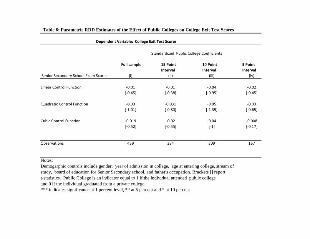
Table 6: Parametric RDD Estimates of the Effect of Public Colleges on College Exit Test Scores

                                                         Dependent Variable:  College Exit Test Scores

                              Standardized  Public College Coefficients  

Full sample 15 Point  10 Point  5 Point 

Interval Interval Interval

 Senior Secondary School Exam Scores (i) (ii) (iii) (iv)

Linear Control Function ‐0.01 ‐0.01 ‐0.04 ‐0.02

[‐0.45] [‐0.38] [‐0.95] [‐0.45]

Quadratic Control Function ‐0.03 ‐0.031 ‐0.05 ‐0.03

[‐1.01] [‐0.80] [‐1.35] [‐0.65]

Cubic Control Function ‐0.019 ‐0.02 ‐0.04 ‐0.008

[‐0.52] [‐0.55] [‐1] [‐0.17]

Observations  439 384 309 167

Notes:Demogarphic controls include gender, year of admission in college, age at entering college, stream of study, board of education for Senior Secondary school, and father's occupation. Brackets [] reportt-statistics. Public College is an indicator equal to 1 if the individual attended public college and 0 if the individual graduated from a private college.*** indicates significance at 1 percent level, ** at 5 percent and * at 10 percent

Soft Skills

Table 7: Parametric RDD Estimates of the Effect of Public Colleges on Soft Skills

Sample restricted to the ‐5 to 5 Interval of Normalized Senior Secondary School Exams Scores

Read Newspaper Use Internet Help Non‐friends Lend Noteswith College Work to Non‐Friends

Public College 0.05 0.07 0.027 ‐0.0008

(0.04) (0.08) (0.08) (0.01)

P ‐value 0.2 0.13 0.8 0.2

N 157 159 157 157 157

Win Any Awards Punished in  Hours Spent  Hours Spent  Number of 

in College College with Students  with Students  Friends in

in Stream out of Stream College

Public College ‐0.09 ‐0.03 0.23* 0.52** 0.56*

(0.11) (0.07) (0.13) (0.2) (0.33)

P ‐value 0.7 0.4 0.08 0.05 0.09

N 154 157 157 157 157

Notes:Demographic controls include gender, year of admission in college, age at entering college, stream of study, board of education for Senior Secondary school, and father's occupation. Robust standard errorsare reported in parenthesis. Public College is an indicator equal to 1 if the individual attended public college and 0 if the individual graduated from a private college.*** indicates significance at 1 percent level, ** at 5 percent and * at 10 percent

Training, Occupation, and Sector

Table 8: Parametric RDD Estimates of the Effect of Public Colleges

Sample restricted to the ‐5 to 5 Interval of Normalized Senior Secondary School Exams Scores

Diploma Post Graduate Professional  Studied or Degree Specialization Worked Aboard

Public College 0.03 ‐0.14 ‐0.16 ‐0.01

(0.09) (0.1) (0.1) (0.03)

P‐value 0.34 0.17 0.128 0.71

N 156 157 159 159

Tertiary  Skill Public Sector Number of Sector Occupation Jobs held

Public College 0.005 0.07 ‐0.12 ‐0.18

(0.08) (0.08) (0.09) (0.15)

P‐value 0.9 0.4 0.17 0.3

N 159 159 158 146

Notes:Demographic controls include gender, year of admission in college, age at entering college, stream of study, board of education for Senior Secondary school, and father's occupation. Robust standard errorsare reported in parenthesis. Public College is an indicator equal to 1 if the individual attended public college and 0 if the individual graduated from a private college.*** indicates significance at 1 percent level, ** at 5 percent and * at 10 percent

Dynamic Learning: Salary, Experience, and Test Scores

Table 9: OLS Estimates of the Effect of Public Colleges on Salary

Dependent Variable: Reported Salary in 6 Categorical Brackets

(i) (ii) (iii) (iv)

Public College 1.08*** 1.09*** 1.6*** 1.5***

(0.19) (0.19) (0.42) (0.4)

Experience 0.31*** 0.38*** 0.45

(0.11) (0.14) (0.3)

Experience Square ‐0.04*** ‐0.04** ‐0.04**(0.01) (0.01) (0.01)

Public * Experience ‐0.2 ‐0.2

(0.2) (0.22)

Public * Experience Square 0.01 0.01(0.02) (0.02)

Senior Secondary Scores * Experience ‐0.001(0.004)

Linear Senior Secondary Scores yes yes yes yes

Observations  419 419 419 419

R‐square 0.23 0.25 0.25 0.27

Notes:Demographic controls include gender, year of admission in college, age at entering college, stream of study, board of education for Senior Secondary school, and father's occupation. Robust standard errorsare reported in parenthesis. Public College is an indicator equal to 1 if the individual attended public college and 0 if the individual graduated from a private college.*** indicates significance at 1 percent level, ** at 5 percent and * at 10 percent

Network Effects: Job Referrals

Table 10: Parametric RDD Estimates of the Effect of Public Colleges on Referrals for Jobs

Sample restricted to the ‐5 to 5 Interval of Normalized Senior Secondary School Exams Scores

Recommended for  Got a job on a  College alumni College alumni a job by a friend referral by a friend at Organization recommended for a job

Public College ‐0.16** ‐0.03 0.027 ‐0.006

(0.074) (0.99) (0.08) (0.07)

N 164 148 136 135

Recommended for  Got a job on a referral  Spouse's College Spouse's college alumni

a job by a friend of  by spouse's friend alumni at recommended for a jobthe spouse Organization

Public College 0.028 ‐0.025 0.11 0.014

(0.7) (0.02) (0.1) (0.1)

N 135 116 120 117

Notes:Demographic controls include gender, year of admission in college, age at entering college, stream of study, board of education for Senior Secondary school, and father's occupation. Robust standard errorsare reported in parenthesis. Public College is an indicator equal to 1 if the individual attended public college and 0 if the individual graduated from a private college.*** indicates significance at 1 percent level, ** at 5 percent and * at 10 percent

Public College Premium and Number of College Friends in the Industry

Table 11: OLS Estimates of the Effect of Public Colleges on Salary

                                                                Dependent Variable: Reported Salary in 6 Categorical Brackets

(i) (ii) (iii) (iv)

Public College 1.13*** 0.57 1.14*** 0.5

(0.22) (0.35) (0.22) (0.36)

Number of Friends from College in the  0.058** 0.008 0.05** 0.002

same Industry (0.028) (0.003) (0.02) (0.004)

Public College * Number of College friends in the  Same Industry 0.1** 0.1**

(0.05) (0.05)

Industry Fixed Effects No No Yes Yes

Observations 358 358 354 354

Notes:Demographic controls include gender, year of admission in college, age at entering college, stream of study, board of education for Senior Secondary school, and father's occupation. Robust standard errorsare reported in parenthesis. Public College is an indicator equal to 1 if the individual attended public college and 0 if the individual graduated from a private college.*** indicates significance at 1 percent level, ** at 5 percent and * at 10 percent

Online Appendix: Supplementary Material

 

 

                       

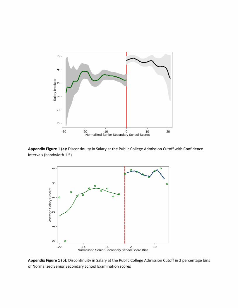
Appendix Figure 1 (a): Discontinuity in Salary at the Public College Admission Cutoff with Confidence 

Intervals (bandwidth 1.5) 

                  Appendix Figure 1 (b): Discontinuity in Salary at the Public College Admission Cutoff in 2 percentage bins 

of Normalized Senior Secondary School Examination scores 

01

23

45

Sa

lary

bra

cke

ts

-30 -20 -10 0 10 20 Normalized Senior Secondary School Scores

01

23

45

Ave

rag

e S

alar

y B

rack

et

-22 -14 -6 2 10 Normalised Senior Secondary School Score Bins

                 Appendix Figure 2: Smooth Density of Forcing Variable 

 

 

0.0

2.0

4.0

6.0

8

-40 -20 0 20 40

Normalized Senior Secondary School Exam Scores

                                       Appendix Figure 3: Smooth Controls 

                      

                      

                               

17.

81

81

8.2

18.

41

8.6

Age

-22 -14 -6 2 10

Normalised Senior Secondary School Score Bins

.1.2

.3.4

.5

Ce

ntr

al B

oa

rd o

f E

du

catio

n

-22 -14 -6 2 10

Normalised Senior Secondary School Score Bins

0.2

.4.6

.8

Ma

les

-22 -14 -6 2 10

Normalised Senior Secondary School Score Bins

                             

                                                        Appendix Figure 3: Smooth Controls continued 

 

 

0.0

5.1

.15

-22 -14 -6 2 10

0.0

5.1

.15

.2.2

5

-22 -14 -6 2 10

0.0

5.1

.15

-22 -14 -6 2 10

0.2

.4.6

-22 -14 -6 2 10

0.0

5.1

.15

.2

-22 -14 -6 2 10

0.2

.4.6

-22 -14 -6 2 10

0.0

5.1

.15

.2.2

5

-22 -14 -6 2 10

Father's Occupation

                

               Appendix Figure 4: Self ‐Reported Assessment of Learning from College Classes 

  

 

 

.8.9

11

.1

Lea

rn F

rom

Co

lleg

e C

lass

es

-30 -20 -10 0 10 20

Normalized Senior Secondary School Exam Scores

                

                                                A: Coefficient of variation = 35.3 

 

                                                            B: Coefficient of Variation = 33.85 

 

   Appendix Figure 5:  Panel A shows the Dispersion in Salary with Experience (0‐6 years) for the Full 

sample. Panel B shows the Dispersion in Salary with Experience near the Admission Cutoff 

12

34

56

sala

ry

0 1 2 3 4 5 6

Dispersion of Salary with Experience

12

34

56

sala

ry

0 1 2 3 4 5 6

(-5 to +5 Interval of SSSE scores)Salary Dispersion with Experience around the Cutoff

 

           Appendix Figure  6: Salary as a function of SSSE Scores for Public Colleges by Years of Experience      

 

 

 

 

 

 

 

 

 

 

23

45

62

34

56

50 60 70 80 90 50 60 70 80 90

0 1 2

3 4 5

Pre

dict

ed

Sal

ary

SSSE Scores

   

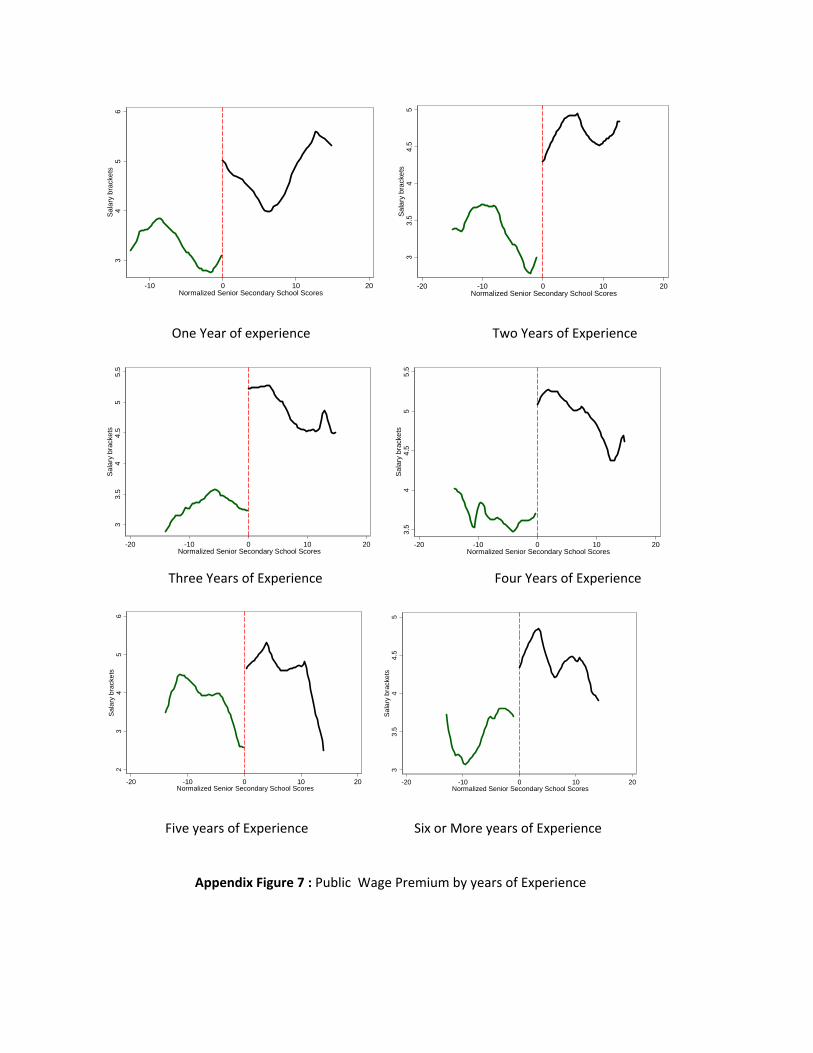
                       One Year of experience                                                       Two Years of Experience 

                         Three Years of Experience                                                    Four Years of Experience 

 

                     Five years of Experience                                Six or More years of Experience 

 

                              Appendix Figure 7 : Public  Wage Premium by years of Experience 

 

34

56

Sa

lary

bra

cke

ts

-10 0 10 20 Normalized Senior Secondary School Scores

33

.54

4.5

5S

ala

ry b

rack

ets

-20 -10 0 10 20 Normalized Senior Secondary School Scores

33

.54

4.5

55

.5S

ala

ry b

rack

ets

-20 -10 0 10 20 Normalized Senior Secondary School Scores

3.5

44

.55

5.5

Sa

lary

bra

cke

ts

-20 -10 0 10 20 Normalized Senior Secondary School Scores

23

45

6S

ala

ry b

rack

ets

-20 -10 0 10 20 Normalized Senior Secondary School Scores

33

.54

4.5

5S

ala

ry b

rack

ets

-20 -10 0 10 20 Normalized Senior Secondary School Scores

                    

       Appendix Figure 8: Binned Average Number of Friends in Industry with Normalized Senior 

Secondary School Examination Scores and Salary Brackets as Cartesian Co‐ordinates 

 

 

 

0

1

2

3

4

5

6

Sa

lary

0 5 10 15 20Normalized Senior Secondary School Scores

0-2.400

2.400 - 5.5005.500 - 7.0007.000 - 11.000> 11.000

Mean Number of Friends in Industry

                                         Appendix Figure 9: Probability of Survey Success 

      

 

                Appendix Figure 10: Discontinuity in Probability of Reporting Salary (IK bandwidth) 

.3.3

5.4

.45

Pro

babl

ity o

f Bei

ng S

urv

eye

d

-20 -10 0 10 20Normalized senior Secondary School Exam Scores

0.2

.4.6

.81

Pro

babi

lity

of

Rep

ortin

g S

ala

ry

-30 -20 -10 0 10 20

Normalized Senior Secondary School Exam Scores

Appendix Table 1: Summary Statistics by College Type in -5 to 5 Interval of Senior Secondary School Normalized Scores

Public Privatemean std dev mean std dev Difference

Salary 5 1 3.55 1.44 1.36***

Senior Secondary School Exam Scores 70.4 8 67.26 7.4 3.2***

Central Board of Secondary Education 0.22 0.42 0.21 0.41 0.01

Age at Starting College 18 0.91 18 0.9 0.08

Father's Occupation

              Government Service 0.1 0.3 0.09 0.28 0.01

              Labor in Unorganized Sector 0.03 0.02 0.06 0.02 0.03

              Professional 0.063 0.24 0.05 0.23 0.006

              Service in Formal Sector 0.35 0.48 0.23 0.42 0.11

               Agriculture 0.075 0.266 0.09 0.29 0.014

                Business 0.25 0.43 0.32 0.47 0.07

Admission Year

1999 0.2 0.4 0.26 0.44 0.05

2000 0.37 0.48 0.19 0.4 0.18***

2001 0.3 0.45 0.26 0.44 0.03

2002 0.12 0.33 0.28 0.45 0.15**

Male 0.46 0.5 0.35 0.05 0.11

Stream

Commerce 0.27 0.45 0.3 0.45 0.016

Liberal Arts 0.51 0.5 0.45 0.5 0.06

Science 0.2 0.4 0.25 0.43 0.047

College Exit Test Scores 1272.35 276 1247 271.2 25.27

Observations 79 88

Appendix Table 2: Ordered Logit Estimation of the Impact of Public Colleges on the Probability of being in a Salary Bracket

Dependent Variable : Salary Brackets

[1] [2] [3] [4] [5] [6]

Average Marginal Effects

Public Colleges

No Controls ‐0.044*** ‐0.15*** ‐0.13*** ‐0.03 0.14*** 0.21***

(0.01) (0.016) (0.02) (0.019) (0.017) (0.038)

Demographic Controls ‐0.044*** ‐0.145*** ‐0.11*** ‐0.013 0.14*** 0.18***

(0.01) (0.016) (0.02) (0.017) (0.017) (0.038)

Demographic Controls and  ‐0.042*** ‐0.14*** ‐0.11*** ‐0.011 0.13*** 0.17***

Senior Secondary School Exam (0.009) (0.02) (0.02) (0.02) (0.018) (0.05)

Scores

Notes:Demographic controls include gender, year of admission in college, age at entering college, stream of study, board of education for Senior Secondary school, and father's occupation. Robust standard errorsare reported in parenthesis. Public College is an indicator equal to 1 if the individual attended public college and 0 if the individual graduated from a private college.*** indicates significance at 1 percent level, ** at 5 percent and * at 10 percent

Selectivity of Colleges- Average Cohort Quality

Appendix Table 3: RDD Estimates of the Effect of the Average Quality of the Students Admitted to Public Colleges on Salary

                                      Dependent Variable: Reported Salary in 6 Categorical Brackets

                                Public College Coefficients from Parametric Regressions in Intervals around the Cutoff 

Full sample 15 Point  10 Point  5 Point 

Interval Interval Interval

(i) (ii) (iii) (iv)

Control Function‐Linear

Without the Cohort Average Senior Secondary 1.05*** 1.02*** 0.95*** 1.2***

School Examination Scores (0.19) (0.2) (0.2) (0.24)

Controlling Cohort Average  Senior Secondary  0.3 0.3 0.34 0.2

School Examination Scores  (0.34) (0.37) (0.4) (0.56)

Control Function‐Quadratic

Without the Cohort Average Senior Secondary 1.08*** 1.04*** 0.96*** 1.18***

School Examination Scores (0.2) (0.2) (0.2) (0.23)

Controlling Cohort Average  Senior Secondary  0.32 0.3 0.34 0.16

School Examination Scores  (0.34) (0.37) (0.4) (0.56)

Control Function‐Cubic

Without the Cohort Average Senior Secondary 1.15*** 1.08*** 0.97*** 1.2***

School Examination Scores (0.2) (0.2) (0.22) (0.24)

Controlling Cohort Average  Senior Secondary  0.38 0.38 0.34 0.1

School Examination Scores  (0.35) (0.38) (0.41) (0.6)

Observations  439 384 309 167

Notes:Demographic controls include gender, year of admission in college, age at entering college, stream of study,board of education for Senior Secondary school, and father's occupation. Robust standard errors clustered at college-stream level are reported in parenthesis. Public College is an indicator equalto 1 if the individual attended public college and 0 if the individual graduated from a private college.*** indicates significance at 1 percent level, ** at 5 percent and * at 10 percent

Public College Premium and Number of College Friends in the Industry

Appendix Table 4: Instrumental variable Estimates of the Effect of Number of College Friends in Industry on Salary

                                                                Dependent Variable: Reported Salary in 6 Categorical Brackets

(i) (ii)

Predicted Number of College Friends in Same Industry 1.6*** 1.22**

(0.55) (0.06)

Covariates No Yes

Observations 371 358Instrument used: Eligibility For Public Colleges 

Notes:

Demographic controls include gender, year of admission in college, age at entering college, stream of study, board of education for Senior Secondary school, and father's occupation. Robust standard errorsare reported in parenthesis. *** indicates significance at 1 percent level, ** at 5 percent and * at 10 percent

Appendix Table 5: Survey Success by College Type in -5 to 5 Interval of Senior Secondary School Normalized Scores

Private Public

Responded  Respondent  Difference Responded  Respondent  Difference

Found not Found Found not Found

Commerce 0.28 0.27 ‐0.01 0.3 0.25 ‐0.04

(0.02) (0.01) (0.02) (0.01)

Science 0.17 0.22 0.04 0.11 0.18 0.07***

(0.02) (0.01) (0.02) (0.016)

Father 0.05 0.086 0.03 0.06 0.06 0.0003

in Agriculture (0.013) (0.01) (0.01) (0.01)

Father 0.19 0.23 0.047 0.27 0.3 0.025

in Service in (0.02) (0.01) (0.02) (0.019)

Formal Sector

Father 0.037 0.03 ‐0.006 0.015 0.03 0.016

in Service in (0.01) (0.007) (0.007) (.007)

Unorganized

Sector

Admission 0.25 0.27 0.013 0.23 0.25 0.02

year 1999 (0.025) (0.018) (0.02) (0.018)

Admission 0.27 0.27 ‐0.006 0.18 0.16 ‐0.02

year 2002 (0.02) (0.018) (0.02) (0.01)

Age at 18.02 18.12 ‐0.1 17.93 18 ‐0.15

Entering (0.09) (0.15) (0.1) (.09)

College

Appendix Table 6: Parametric RDD Estimates of the Effect of Public Colleges on being Employed

                                      Dependent Variable: Self Employed or Working for Salary

                                Public College Coefficients from Parametric Regressions in Intervals around the Cutoff 

Full sample 15 Point  10 Point  5 Point 

Interval Interval Interval

 Senior Secondary School Exam Scores (i) (ii) (iii) (iv)

Linear  0.05 0.06 0.03 0.06

(0.03) (0.04) (0.04) (0.05)

Quadratic  0.05 0.06 0.04 0.067

(0.03) (0.04) (0.04) (0.053)

Cubic 0.04 0.06 0.03 0.05

(0.036) (0.04) (0.04) (0.05)

Observations  1505 1285 1017 549

Notes:Demographic controls include gender, year of admission in college, age at entering college, stream of study, board of education for Senior Secondary school, and father's occupation. Robust standard errorsare reported in parenthesis. Public College is an indicator equal to 1 if the individual attended public college and 0 if the individual graduated from a private college.*** indicates significance at 1 percent level, ** at 5 percent and * at 10 percent

Appendix Table 7: Characteristics of Individuals who report their salary and those who do not

Salary Reported Salary not Reported Difference

Senior Secondary School Exam Scores 66.57 66.35 ‐0.21

(0.48) (0.63)

Age at Entering Colleges 18.03 18.15 0.12*

(0.046) (0.04)

Admission Year 1999 0.21 0.26 0.04

(0.02) (0.02)

Admission Year 2000 0.29 0.3 0.01

(0.02) (0.02)

Admission year 2001 0.24 0.02 ‐0.03

(0.02) (0.02)

Admission year 2002 0.24 0.23 ‐0.017

(0.02) (0.02)

Central Board of Secondary Education 0.31 0.25 0.06*

(0.02) (0.02)

Male 0.4 0.78 0.38***

(0.023) (0.02)

Father's occupation

Government Service 0.08 0.04 ‐0.04**

(0.01) (0.01)

Labor in Unorganized Sector 0.07 0.05 ‐0.02

(0.01) (0.01)

Professional 0.05 0.02 ‐0.03**

(0.01) (0.008)

Service in Formal sector 0.3 0.25 ‐0.067**

(0.02) (0.02)

Agriculture 0.07 0.06 ‐0.007

(0.01) (0.01)

Business 0.3 0.36 0.07**

(0.02) (0.03)

Streams

Commerce 0.24 0.35 0.1***

(0.02) (0.03)

Liberal Arts 0.51 0.57 0.06*

(0.02) (0.03)

Science 0.24 0.06 ‐0.17***

(0.02) 0.01

*** indicates significance at 1 percent level, ** at 5 percent and * at 10 percent

Appendix Table 8: Bounded Effect of Public Colleges on Salary

                       Dependent Variable: Reported Salary in 6 Categorical Brackets

‐5 to +5 Interval

Full sample around cutoff

Number of Observations  748 274

Number of Observations with Non Missing Salary 458 171

Trimming Proportion 0.1865 0.1947

Confidence Interval for the Treatment Effect [95%] [0.443  1.9] [0.503  2.3]

Lower Bound

Coefficient 0.73*** 0.96***

Standard Error (0.17) (0.27)

95% confidence Interval

Upper Bound

Coefficient 1.6*** 1.86***

Standard Error (0.17) (0.27)

95% confidence Interval

*** indicates significance at 1 percent level, ** at 5 percent and * at 10 percent