Presidential popularity in a young democracy:

Russia under Yeltsin and Putin

In established democracies, voters often evaluate incumbents’ performance based on economic outcomes. By contrast, in young democracies leaders are often thought to seek support by exploiting nationalism, exaggerating external threats, and manipulating the media. Such ploys are believed to work because voters are inexperienced and unsophisticated. Using time series data, I examine the determinants of presidential popularity in Russia since 1991, a period in which leaders’ ratings swung between extremes. I find that Yeltsin’s and Putin’s ratings were, in fact, closely linked to public perceptions of economic performance, which, in turn, tracked objective economic indicators. Although media manipulation, wars, terrorist attacks, and other events had some effect, Putin’s unprecedented popularity and the decline in Yeltsin’s are well explained by the contrasting economic circumstances over which each presided. In some transitional democracies, the volatility of leaders’ popularity may reflect not the capriciousness of citizens but logical responses to economic volatility.

Daniel Treisman

Department of Political Science University of California, Los Angeles

4289 Bunche Hall Los Angeles California 90095

treisman@polisci.ucla.edu

November, 2009

I thank Yevgenia Albats, Robert Erikson, Lev Freinkman, Tim Frye, Scott Gehlbach, Vladimir Gimpelson, Sergei Guriev, Arnold Harberger, John Huber, Rostislav Kapelyushnikov, Matthew Lebo, Grigore Pop-Eleches, Brian Richter, Richard Rose, Jim Snyder, Konstantin Sonin, Stephen Thompson,

Jeff Timmons, Josh Tucker, Andrei Yakovlev, Alexei Yudin, Katya Zhuravskaya and other participants in seminars at the Higher School of Economics, Moscow, and Columbia University for comments or helpful

communications.

1 Introduction

The essence of modern democracy is the use of elections to select effective leaders and motivate them to

act in the public’s interest. In the developed democracies of the West, voters are often thought to judge

incumbents on the basis of economic conditions, rewarding those who preside over prosperity and

punishing those whose terms coincide with economic deterioration. In this, the voters are considered

rational. Imperfectly informed about the state of the world, they decode signals about the competence of

officials from the economic statistics and vote accordingly (e.g. Rogoff and Sibert 1988).

Can—and do—voters in young democracies exercise a similar control over their leaders,

sanctioning the incompetent on the basis of economic performance?1 In the view of some scholars and

commentators, various obstacles make this difficult. Socialization into authoritarian regimes is thought to

have left citizens of young democracies psychologically ill-equipped for such a role. Drawn to “strong”

leaders, sensitive to nationalist appeals, poorly informed and unorganized, they are seen as easily

manipulated by government advertising on state-dominated media, and more likely to focus on image and

personalities than to soberly evaluate performance by studying economic statistics. Cynical about the

system’s responsiveness, citizens may also, quite reasonably, give up on sanctioning ineffective leaders

(Duch 2002). In this environment, incumbents are tempted to exaggerate external threats, warn of terrorist

dangers, or even begin military engagements to generate rallies of support (Mansfield and Snyder 1995).

One country where these issues arise particularly starkly is Russia. Since the first competitive

presidential election there in 1991, presidents’ approval ratings have careened wildly. Russia’s first

president, Boris Yeltsin, started out extremely popular, with 81 percent of Russians approving of his

performance in September 1991. By the time he left office eight years later, that proportion had dropped

to eight percent.2 His successor, Vladimir Putin, relatively unknown a few months before, saw his

1 Of course, voters can only control their governments to the extent that elections are not too fraudulent. I leave that issue to one side here to focus on the question whether citizens in young democracies—specifically Russia—evaluate leaders on the basis of economic performance. 2 Data from polls by VCIOM, available at http://sofist.socpol.ru.

2

approval shoot up from 31 percent in August 1999 to 84 percent in January 2000. In his eight years as

president, his rating rose as high as 87 percent and never fell below 60 percent.

To some, these extreme swings reveal the country’s political immaturity. Journalists attributed

both wars in Chechnya to the desire to boost a Kremlin-backed candidate’s electoral prospects. Putin’s

popularity has been explained as the result of an artificially cultivated image as a “tough” leader, the

trauma after terrorist bombings in late 1999, and the Kremlin’s increasing control and manipulation of the

media. Such interpretations seem in accord with the fluidity of the political scene, where parties have

come and gone and politics has often been seen as primarily the clash of personalities.

But there is another possibility. The volatility of presidents’ ratings and vote shares could merely

mirror volatility in the economy. Russians might be responding to perceived conditions in a manner as

logical as their Western counterparts. The swings in incumbents’ approval might reflect not Kremlin

manipulation or the flightiness of voters but their admittedly crude attempts, in an environment of

uncertainty and imperfect information, to hold their leaders to account.

Although there are many conjectures about what causes change over time in the popularity of

Russian presidents, few have attempted to confront these systematically with evidence.3 In this paper, I

use statistical techniques and time series survey data to do so. I look first at what polls reveal directly

about the determinants of presidential popularity. Then, with error correction regression models, I test

whether factors related to various arguments help predict the trajectories of presidents’ ratings.

Understanding what influences presidential approval in Russia is important for several reasons.

Not least, it has practical implications for Russian politics. If building support for an incumbent requires

only the projection of a particular image, it makes sense for the Kremlin’s operatives to monopolize the

mass media. If Putin’s appeal was boosted by the struggle against Chechen terrorists, such threats are

likely to be dramatized as elections approach. However, if what mattered was the economic recovery,

implications are more benign: leaders will need to master the nuts and bolts of economic management.

3 Mishler and Willerton (2003) is a notable exception. By contrast, a number of scholars have examined what characteristics of individual Russians best explain their rating of the president at a given moment in time.

3

Determining the influence of economics is also important to assess the likely impact of the 2008-9

financial crisis on the evolution of democracy in Russia.4

Although Russia is unique in certain regards, and conclusions can not be generalized

unreflectively, the results suggest hypotheses and modes of analysis relevant to other young democracies.

Debates continue over the influence of economics and charismatic populism over election results and

presidential approval in Latin America.5 Does Hugo Chavez’s appeal in Venezuela rest on ideological

support for his “Bolivarian Revolution” or on oil-fueled prosperity? Did the popularity of Fujimori in

Peru owe more to economic conditions or his counterinsurgency efforts (Arce 2003)? Scholars have also

pondered what shapes presidential popularity in the young democracies of Asia, exploring, for instance,

whether the dips in Indonesian President Yudhono’s rating in 2008 were caused by falling oil prices or by

the image of the president as “weak, indecisive, and increasingly defensive” (Mietzner 2009, p.147).

To preview the results, I find that Russians are surprisingly like voters in developed democracies

in how they judge their leaders. Their evaluations closely follow economic conditions. Perceptions of the

state of the Russian economy and of families’ own finances do a good job of predicting both the decline

in Yeltsin’s rating, and the surge and plateau in Putin’s. Although leaders have tried to manipulate

perceptions, the statistical evidence suggests such efforts have had quite limited effects. At times—

notably during certain election campaigns—Russians’ views of the economy were rosier than warranted.

But in general economic perceptions were well predicted by objective economic indicators.

On balance, the evidence suggests that much commentary and analysis of recent Russian politics

has exaggerated the importance of the style and image of leaders. At the same time, the Chechen wars

appear to have weighed on presidential approval most of the time. Although the outbreak of the second

war may help account for Putin’s sudden surge in late 1999, from then on the war reduced his popularity.

His rating rose in 2005-7 as Russians came to believe the Chechen situation was stabilizing.

4 And, of course, Putin remains as prime minister, believed by many to be making the key decisions, together with his loyal aide—and now the country’s president—Dmitri Medvedev. His return to presidential politics is widely expected in 2012. Thus, the causes of his popularity are of more than historical interest. 5 See, for instance, Dominguez and McCann (1996), Weyland (2003).

4

In this paper, I study what determines change in the average level of support for Russian

presidents over time. A number of other papers, using cross-sectional survey data, have explored what

characteristics of individuals correlated with support for Yeltsin or Putin at given moments. Such studies,

like this one, tend to find that economic factors were important (Duch 1995, Miller, Reisinger, and Hesli

1996, Hesli and Bashkirova 2001, Rose, Mishler and Munro 2004, Rose 2007b, Colton and Hale 2008;

White and Mcallister 2008). While this correspondence is reassuring in a way, it is important to remember

how cross-sectional and time series analyses differ. They do not, as sometimes thought, generate

comparable, potentially competing evidence on the same question. Rather, they address different

questions. Cross-sectional analyses uncover what types of citizens favored the incumbent at a given

moment. They reveal little about the level of and changes in total support. For this, we need time series or

panel data and analyses. To see this, suppose all citizens’ incomes doubled simultaneously, causing a

massive surge of approval of the president. A cross sectional regression would find no relationship

between individuals’ change in income and support for the president since there would be no variation

across individuals in the income change—and it is variation across individuals that cross-sectional

regressions pick up.6 Of course, time series regressions are unable to answer the other type of question—

about the importance of characteristics that vary across individuals but not over time.7

The only time series analysis of Russian presidential approval of which I am aware is Mishler and

Willerton (2003), which examined data up to 2000, and so was not able to draw strong comparisons

between the Yeltsin and Putin periods. I extend their analysis in various ways, and, using the more

extensive data now available, draw somewhat different conclusions.

6 The problem does not necessarily disappear if the income change is not identical for all individuals. The common element in the income change may still have a much stronger impact on opinion than the cross-respondent variation. And the cross-respondent variation may not be large enough to estimate the over time effects. 7 For an excellent discussion of the different uses of cross-sectional and time series data, see Erikson, MacKuen and Stimson (2002). In addition, average opinion may be more informative and well-behaved than the opinion of individuals because idiosyncratic or random elements tend to balance each other out. In the American context, knowledge of the individual voter “turns out not to be a reliable guide for generalizing to the electorate and its role in democratic politics.”

5

2 Data on presidential approval

The main data I analyze come from a regular, face-to-face survey conducted by the Russian Center for

Public Opinion Research (VCIOM) until September 2003, and then by its successor, the Levada Center.8

VCIOM, founded in 1988, was directed from 1992 by Yuri Levada, a sociologist who had been fired from

Moscow State University in 1969 for “ideological mistakes in his lectures.” VCIOM acquired a reputation

as the most professional and politically independent of Russia’s half dozen leading polling organizations.

This independence is believed to have prompted a hostile state takeover in 2003, in which Levada was

dismissed. The center’s researchers set up the private Levada Center, which continued the polls.

The surveys are of a nationally representative sample of voting-age citizens, who are interviewed

in their homes. I focus on two questions. First, the pollsters ask: “On the whole do you approve or

disapprove of the performance of Boris Yeltsin [after December 1999, Vladimir Putin]?” This question,

similar to that posed by the US Gallup poll, was included monthly from late 1996 (and irregularly before

then).9 I use it to examine approval of President Putin, first elected in March 2000. However, since this

question was asked only occasionally before September 1996, I use another to study Yeltsin’s popularity.

This one, included every second month from early 1994 (and less regularly before then), asked: “What

evaluation from 1 (lowest) to 10 (highest) would you give the President of Russia Boris Yeltsin?”10 I use

the average evaluation as a measure of Yeltsin’s approval.11 In months for which both measures are

8 Mishler and Willerton (2003) studied a subset of these data, for Yeltsin’s presidency and the first 18 months of Putin’s. 9 The US Gallup poll asks: “Do you approve or disapprove of the way that [President's name] is handling his job as President?” 10 This question was also used by Mishler and Willerton (2003). In the approval question, sample sizes were about 1600; in the 10-point scale questions, the size was usually from 2,100 to about 2,400. 11 I construct a dataset including just the alternating months in which the question was asked, from early 1994 when the regular series began. In a previous version of the paper, I had interpolated the missing values linearly. However, this required interpolating about 50 percent of the data, which might inflate the significance of estimates and increase autocorrelation. Although it turns out that whether or not one interpolates the missing months does not affect the results much, here I use the bimonthly series. I also use a bimonthly series to analyze the Putin period, even though the appproval question was asked monthly, in order to avoid having to interpolate a large amount of data for the key economic explanatory variables, which were available only every second month.

6

available, the two are highly correlated, both in levels (r = .98) and in two-month differences (r = .91).12

The data are shown in Figure 1. On the left, Yeltsin’s rating bumps its way down from its 1991

peak. On the right, we see Putin’s remarkable eight years with approval consistently above 60 percent. No

American president has equaled this since regular polling began in the 1930s. Eisenhower came closest,

but even his rating fell into the 50s and even the 40s.13 No British prime minister has come close at least

since the first MORI poll in 1979.14

12 The correlation for levels includes all months in which both were available between January 1992 and March 2008; that for 2-month differences, the period for which a virtually complete bimonthly series existed for both (September 1996 - March 2008). 13 I base this on the Gallup poll, the historical data from which are available at the American Presidency Project, at http://www.presidency.ucsb.edu/data/popularity.php.

0

10

20

30

40

50

60

70

80

90

100

0

1

2

3

4

5

6

7

8

9

10

1991 1992 1993 1994 1995 1996 1997 1998 1999 2000 2001 2002 2003 2004 2005 2006 2007 2008

Figure 1.   Presidential Approval, Russia 1991‐2008

Yeltsin rating on 10 point scale, left axis Putin rating on 10 point scale, left axis

Yeltsin approval, %, right axis Putin approval, %, right axis

Sources: See appendix. Surveys of VCIOM and Levada Center. Yeltsin approval is percentage of respondents saying on the whole they approve of the peformance of Boris Yeltsin. Likewise for Putin approval. Ratings on 10 point scale are average answer to: "What evaluation from 1 (lowest) to 10 (highest) would you give the President of Russia (name of president)?" Putin approval includes his period as prime minister.

7

A natural first question, then, is whether the results are believable. Might Putin’s high ratings

have been concocted to please the Kremlin or reflect the insincere replies of intimidated respondents?

There are reasons to feel reassured on these points. First, it is hard to believe VCIOM was slanting its

results to please Putin given its leaders’ impeccable credentials and the state’s takeover of the center in

2003 to punish it for insufficient loyalty. Various Western polling teams (such as World Public Opinion

and the New Russia Barometer) have worked with the Levada group and found it highly professional. It is

also reassuring that the dynamics in the VCIOM/Levada polls are very close to those in surveys by other

organizations. For instance, the Levada 10-point scale rating correlates at r = .93 with the proportion of

respondents to polls by the Fond Obshchestvennogo Mnenia that said they “trusted” Putin in 2006-7.15

Second, it seems unlikely many respondents were scared to answer frankly given their readiness

to express harsh criticism on other questions. Asked in 2004 whether there was more or less corruption

and abuse of power in the highest state organs than a year before, 30 percent said “more,” 45 percent said

“the same amount,” and only 13 percent said “less.”16 Respondents were not shy to give Yeltsin a six

percent approval rating and Putin just 31 percent in 1999. Even as Russians swooned over Putin, his

governments never won the approval of more than 46 percent of respondents, and large majorities

opposed ome of his policies, including—after the initial period—the military occupation of Chechnya.17

Another concern is that, by limiting respondents to a 10 point scale, the surveys are censoring the

data (this issue does not arise for the approval measure). Some might have liked to give Yeltsin less than

14 See the Ipsos-MORI polls at http://www.ipsos-mori.com/polls/trends/satisfac.shtml. 15 The FOM data are available on its website at www.fom.ru. 16 Results at www.russiavotes.org, Slide 450. Twelve percent picked “don’t know.” 17 Wyman (1997, pp.5-19) includes an excellent discussion of the difficulties and common criticisms of polling in Russia, and concludes that most problems are those faced by survey researchers worldwide. Beyond the positivity bias that makes respondents everywhere more likely to answer yes than no, “there is no evidence specific to Russia that respondents…. engage in self-censorship.” To assess whether respondents were afraid to give critical opinions, Rose (2007) asked respondents in 13 postcommunist countries in 2004-5 whether they thought “people today are afraid to say what they think to strangers.” Among Russian respondents, 25 percent thought people were afraid to some extent, while 74 percent thought they were not. This was the lowest reported fear level for all 13 countries. He also found that those who did think people were afraid to say what they think to strangers—and who presumably were somewhat afraid themselves—were only very slightly more likely to favor the current regime, suggesting distortions due to self-censorship are minor. See, also, the discussion in Rose, Mishler, and Munro (2007, pp.73-4).

8

one. In the appendix, I show the distributions of responses around Yeltsin’s highest and lowest points.

While the distribution is reasonably symmetric for Yeltsin’s peak, respondents did cluster at the bottom

around his low point. To the extent the end of the scale was censoring some respondents, the effect of

economic decline under Yeltsin may actually have been stronger than that which I estimate.

3 Possible explanations

To assess arguments about presidential approval, I look first at polls bearing directly on the plausibility of

the hypothesis and then run time series regressions to see whether related variables help to predict the

ratings. I treat the two presidencies separately because, examining Figure 1, it seems likely the underlying

process changed between their tenures.18

3.1 Chechnya and terrorism

In other countries, the public often rallies behind leaders at the start of wars (Mueller 1973). Both Russian

wars in the southern republic of Chechnya began in the runup to presidential elections. In November

1994, Yeltsin’s aide Oleg Lobov reportedly said that a “small, victorious war” in Chechnya was needed to

“raise the president’s ratings.”19 Putin’s early rise in the polls occurred as he sent troops to the republic for

a second time and promised to destroy the terrorists who had bombed four Russian apartment buildings.

Many saw it as a traditional wartime rally. “People believed that he, personally, could protect them,”

Yeltsin wrote in his memoirs. “That’s what explains his surge in popularity” (Yeltsin 2000, p.338).

Surveys suggest the public viewed the two wars quite differently. Yeltsin’s use of force in

December 1994 was widely condemned. In January 1995, two thirds or more of Russian respondents

18 And analysis using the 10-point scale for both periods (not shown here) confirms that the coefficients on key variables changed between the two presidencies. Economic perceptions, although still highly significant, had somewhat smaller coefficients under Putin. It is intuitive to suppose that Russians acclimated psychologically to the stable growth under Putin and were less sensitive to short run changes than they were to the large, sustained, irregular economic declines under Yeltsin. 19 Colton (2008, p.290) reports that Lobov later denied having made this comment, although he did admit to overestimating the chances of a quick success.

9

opposed it (Jeffries 2002, p.372). By summer, 71 percent disapproved of Yeltsin’s actions regarding

Chechnya; only 16 percent approved. However, by 1999 opinion had soured on the compromise of

August 1996, under which the government of president Aslan Maskhadov failed to prevent terrorists from

crossing the border to take hostages for ransom. In October 1999, 74 percent supported a major military

operation against illegal armed groups in Chechnya.20 Asked what attracted them about Vladimir Putin,

the second most popular answer that month—with 24 percent—was “I support his policy on Chechnya.”

However, backing for Putin’s approach proved fickle. By July 2000, about two thirds of Russians

thought Putin’s attempts to rout the insurgents mostly or completely unsuccessful, and the share remained

above 60 percent until 2006. By November 2000, more Russians thought the government should start

peace negotiations than thought it should continue the military operation. And by early 2001, fewer than

one in ten respondents said they were attracted to Putin by his Chechnya policy. If Putin’s hard line on

Chechnya helped him in his early months in power, this does not seem to have been the case later on.

3.2 Personal style

Some saw the main reason for Putin’s popularity and Yeltsin’s dwindling appeal in their divergent

personal styles. Yeltsin—ailing, gaffe-prone, at times visibly inebriated—could hardly have seemed more

different from the disciplined, energetic, sober Putin, a former spy and judo black belt. As one Russian

journalist put it: “He is, if you like, our James Bond.”21 Polls confirm that Russians were attracted by

Putin’s image of youthful vigor and put off by Yeltsin’s physical decline. When asked what qualities they

found attractive about Putin, from 30 to 47 percent of respondents chose “he is an energetic, decisive,

strong-willed person.” Only nine percent said this of Yeltsin in January 2000. Even in 1996, the third

most frequent thing respondents disliked about Yeltsin was that he was “a sick, weak person.”22

20 VCIOM, Omnibus poll 1995-4, 11 July – 10 August, 1995, 2,983 respondents, at http://sofist.socpol.ru; VCIOM, Express poll, 1999-11, 29 Oct – 2 Nov, 1999, 1,600 respondents, at http://sofist.socpol.ru. 21 Vladimir Soloviev, quoted by Andrew Harding, “Why is Putin Popular?”, BBC News, 8 March, 2000. 22 VCIOM Express 1996-3, 15-20 February, 1996, 1,584 respondents, at http://sofist.socpol.ru.

10

But did the presidents’ images explain their varying levels of support? Unfortunately, regular data

were not available to test this hypothesis systematically. The VCIOM/Levada pollsters did periodically

ask respondents “What attracts you about Vladimir Putin?” allowing them to choose answers from a list. I

considered using a time series of the proportion saying they were attracted to Putin by his energy,

decisiveness and strong will. However, the question was only asked in 19 of the 96 months between

January 2000 and December 2007, so this would have required interpolating massive amounts of data.

Governing style is also manifested in particular incidents. One episode thought to have

punctured Putin’s image of decisiveness was his insensitive reaction when the Kursk nuclear submarine

sank in the Barents Sea in 2000. While the Navy brass ignored offers of Western help and delayed

mounting a rescue mission, Putin was shown on the news jet-skiing on the Black Sea. As for Yeltsin, his

image cannot have benefited from his frequent hospital stays (Mishler and Willerton 2003). Yeltsin’s

drinking problem was most vividly illustrated in August 1994, when television showed him energetically

conducting a police band in Berlin. I created dummies for each of these to include in the regressions.

3.3 Imposing order

From the start, Putin promised to restore “order” after the turbulent 1990s, to fight crime and corruption,

and to reimpose central control over wayward local officials. A former KGB officer, he seemed to have

the appropriate experience and connections. Could this explain his popularity?

Many—perhaps a growing proportion of—Russians say in surveys that they favor strong leaders

and are willing to sacrifice some civil or political rights in return for order.23 However, it turns out that

23 Whether this reveals a cultural predilection for authoritarian rule or just a response to extreme conditions is hard to say. After the terrorist attacks of 9/11, large majorities of American and British respondents were willing to compromise civil liberties to increase domestic security. In a YouGov poll of a representative sample of British adults, 70 percent said they were “willing to see some reduction in our civil liberties in order to improve security in this country” (“Observer Terrorism Poll: Full Results,” The Observer, September 23, 2001). A New York Times/CBS poll around the same time found 64 percent of US respondents thought that in wartime “it was a good idea for the president to have authority to change rights usually guaranteed by the Constitution” (Robin Toner and Janet Elder, “A Nation Challenged: Attitudes; Public is Wary but Supportive on Rights Curbs,” New York Times, December 12, 2001). See, also, Hale (2009) for a convincing debunking of the common claim that Russians are undemocratic.

11

those who favored a “strong hand” and other antidemocratic norms were generally less likely to support

Putin than the Communist leader Gennady Zyuganov or the ultranationalist Vladimir Zhirinovsky. In fact,

Whitefield (2005) found it was supporters of democracy that favored Putin.24

At the same time, Russians were quite skeptical of Putin’s claims. Roughly twice a year between

2000 and 2007, VCIOM/Levada polls asked how successful Putin had been recently in imposing order in

the country. On average 47 percent thought he had been at least partly successful, while 49 percent

thought he had been unsuccessful.25 There was no clear trend. When asked more specific questions, those

reporting deterioration vastly outnumbered those reporting improvement. Each year since 2000, at least

25 percent more thought citizens’ personal security had worsened than thought it had increased. Each

year, at least 15 percent more saw deterioration in law enforcement than saw improvement.26 At the start

of his term, 29 percent said they were attracted to Putin because he was “someone who could impose

order in the country.” By October 2006 the share had fallen to 13 percent. For the regressions, I used a

measure of the percentage of respondents who thought Putin had been very or quite successful in creating

order in the country minus the percentage who thought he had been mostly or completely unsuccessful.

Since this question was asked only 14 times, this required shortening the data period and interpolating

two thirds of the data. Perhaps for this reason, the measure was not statistically significant.27

Following Mishler and Willerton (2003), I created a measure of respondents’ assessments of the

political situation from a question asked roughly bimonthly: “Overall, how would you assess the political

situation in Russia?” I subtracted the proportion choosing “critical, explosive,” and “tense” from the share

choosing “calm” and “favorable.” This variable turns out not to be significant in the regressions. (In any

case, causal modeling presented in the appendix suggests that this measure of the political mood was 24 This was confirmed by a Pew Research Center poll that asked a similar question and again found Putin’s approval was lower among those favoring a leader with a “strong hand” (Morin and Samaranayake 2006). Rose, Mishler, and Munro (2004) also found that support for Putin did not predict support for undemocratic forms of government. 25 See “Prezident: otsenki dyeatelnosti,” Levada Center, at http://www.levada.ru/ocenki.html. 26 Levada Center press release, at http://www.levada.ru/press/2007120703.html. 27 I include this and the variable on international affairs with some reservations given the very large amount of interpolation necessary; however, some previous readers of the paper thought it important to do so.

12

itself caused in part by economic expectations. The political mood was highly correlated to both

perceived current economic performance and perceptions of the state of affairs in Chechnya.)

To test whether Putin’s attacks on the oligarchs earned him support, I created a dummy for the

month after Khodorkovsky’s arrest. To see if Putin gained by indulging nostalgia, I constructed a dummy

for his restoration of the Soviet music to the national anthem. Polls at the time found a large plurality—46

percent in a VCIOM poll, 50 percent in one by ROMIR—in favor of the Soviet Alexandrov version.28

3.4 Foreign affairs

In surveys, respondents regularly graded Putin very highly on “strengthening Russia’s international

position.” Between July 2000 and March 2007, 65 percent of respondents on average said he was coping

with this quite or very successfully, compared to 47 percent who said this of his efforts to “introduce

order in the country,” and 41 percent who saw him as successful in “defending democracy and political

freedoms.”29 By contrast, many thought Yeltsin had been too accommodating towards the West, which

expanded NATO into Eastern Europe on his watch and then bombed the Serbs over Kosovo.

To capture effects of foreign affairs, I included variables for the 9/11 attack in the US, which was

followed by a spike in sympathy for the US among Russians (Putin was the first foreign leader to reach

President Bush to offer sympathy and support), for the NATO bombing of Kosovo, and for the 2003 US

invasion of Iraq. Both Western military actions were unpopular in Russia and might have reduced support

for presidents viewed as too cozy with Washington. Under Putin, I also included the percentage that

thought Putin was successfully strengthening Russia’s international position minus the percentage that

thought he was mostly or completely unsuccessful in this. These results need to be treated very cautiously

as including this variable required shortening the time series and interpolating two thirds of the data

28 VCIOM Express poll, 2000-22, 27-30 October, 2000, 1,600 respondents, and Romir Omnibus poll, 2000-11, 1-30 November, 2000, 2,000 respondents. Results available at http://sofist.socpol.ru. In a previous version of the paper, in which I interpolated more data, I was able to examine the effect of public reactions to the moments of constitutional crisis in April and October 1993. Foregoing such interpolation, available data now begin in 1994. 29 See http://www.levada.ru/ocenki.html.

13

points. The variable was not significant, perhaps because of these data problems.

3.5 Media coverage

To his opponents, Putin’s ratings simply reflected the Kremlin’s increasing dominance of the press. In

the words of Garry Kasparov: “You cannot talk about polls and popularity when all of the media are

under state control” (Remnick 2007). Under Putin, state companies or loyal businessmen took over the

last independent national television networks. Strong criticism of the president—although not of the

government—largely disappeared from mainstream broadcasts. Based on a 1999 survey, White et al.

(2005, p.192) concluded that bias in the official media played a major role in Putin’s rise: “The decisive

factor in this dramatic reversal of fortunes appeared to be the media, particularly state television.”

Constructing a measure of change in press freedom over time was difficult. For lack of a more

sophisticated measure, I used the organization Freedom House’s annual index of press freedom, with the

annual value used for each month of the relevant year. I also created a variable for the month of the state

takeover of NTV, the network previously most critical of the Kremlin.

3.6 Economics

Economic performance—and, especially, perceptions of it—have been shown to influence approval of

incumbents in countries such as the US, France, and Britain (Erikson, MacKuen and Stimson 2002, Lafay

1991, Clarke and Stewart 1995, Sanders 2000). In Russia, too, scholars have found economic influences

on voting (Colton 2000, Tucker 2006). Recent economic performance might also influence presidential

popularity. Such effects might be retrospective or prospective, and might focus on respondents’ own

circumstances or their view of conditions nationwide.

Previous analyses from Russia and other post-Soviet countries found evidence of all four types of

economic influences. Hesli and Bashkirova (2001), looking at cross-sectional surveys, found all four

effects shaped support for Yeltsin. Mishler and Willerton (2003), focusing on time series data, noted the

14

influence of retrospective evaluations of both the national economy and family finances. Rose et al (2004,

p.209) also found in a cross-section that respondents’ views of current economic performance were the

strongest predictor of support for the political regime.

Data were available in the VCIOM/Levada surveys to construct three variables. For retrospective

evaluations of the national economy, I use the question: “How would you assess Russia’s present

economic situation?” For retrospective assessments of personal finances, I use the question: “How would

you assess the current material situation of your family.” In both cases, respondents could answer “very

good,” “good,” “in between,” “bad,” “very bad,” or “don’t know.” I subtracted the shares saying “very

bad” or “bad” from those saying “very good” or “good.” For prospective evaluations of the national

economy, I use the question: “What do you think awaits Russia in the economy in the coming several

months?” Respondents chose between “a significant improvement of the situation,” “some improvement

of the situation,” “some deterioration of the situation,” “a significant deterioration of the situation,” and

“don’t know.” I subtracted the percentage anticipating deterioration from that anticipating improvement.30

Unfortunately, no question was available to measure prospective evaluations of personal finances for a

comparable period. I also created a dummy to capture the extreme shock of the August 1998 crisis.

4 Explaining presidential approval: analysis

Before analyzing the patterns in presidential ratings, some statistical issues must be addressed. As is well-

known, OLS regressions on non-stationary data may produce spurious results. I began, therefore, by

examining whether the approval data and the time series explanatory variables were stationary, i.e. I(0);

had a unit root, i.e. I(1); or were something in between, i.e. fractionally integrated, I(d) where

0 < d < 1.31 Table 1 shows test statistics for the main series in the Yeltsin and Putin periods, using the

30 These variables were available in a continuous bimonthly series from early 1994, and irregularly before then. In a previous version of the paper, I included some observations from 1993, but I have eliminated these because they required interpolating data. Results are very similar including them. 31 On the analysis of fractionally integrated time series, see, for instance, Box-Steffensmeier and Smith (1996).

15

augmented Dickey-Fuller (ADF) and the Phillips-Perron tests to test the null hypothesis of a unit root, and

the Kwiatkowski et al. (KPSS) and Harris-McCabe-Leybourne (HML) tests to test the null of stationarity.

Table 1.   Testing for stationarity, unit roots, and cointegration 

              A. Under Yeltsin (May 1994 ‐ Dec 1999, bimonthly data) 

    Yeltsin rating  Current economy  Family finances  Russia’s ec. future  Political situation 

           ADF test of I(1)  

‐1.26,  p < .90  ‐2.17, p < .90  ‐2.00, p < .90  ‐2.47, p < .90  ‐2.43, p < .90 

Phillips‐Perron test of I(1)  

‐1.22, p < .90  ‐1.97, p < .90   ‐2.39, p < .90  ‐2.56, p < .90  ‐2.58, p < .10 

KPSS test of I(0)  

.03, p < 1  .00, p < 1  .02, p < 1  .01, p < 1  .00, p < 1 

HML test of I(0)  

2.24, p = .01  2.22 p = .01  2.19, p = .01  2.04 p = .02  2.23 p = .01 

Estimate of d  0.884 (.17)  .909 (.17)  0.977 (.17)  0.505 (.17)  0.553 (.17)            Estimate of d for residuals of regression of Yeltsin rating on this variable 

 

0.344 (.17)   0.509 (.17)  0.629 (.17)  1.001 (.17) 

  B. Under Putin (Jan 2000 ‐ Nov 2007 or Mar 2008, bimonthly data)   

  Putin approval   Current ec.  Family finances Russia’s ec. future War in Chechnya  Pol. situation 

             ADF test of I(1)  

‐1.99, p <.90  .11, p < .98  ‐.85, p < .90  ‐2.09, p < .90  ‐1.18, p < .90  ‐.09, p < .95 

Phillips‐Perron test of I(1)  

‐2.78 p < .10  ‐.68, p < .90  ‐1.80, p < .90  ‐3.10, p < .05   ‐.28, p < .95  ‐.95, p < .90 

KPSS test of I(0)  

.00 p < 1  .14, p < 1  .07, p < 1  .15, p < 1  .10, p < 1  .34, p < 1 

HML test of I(0)  

2.49, p = .01  2.35, p =.01  2.42,p = .01  ‐.17, p = .57  3.32, p = 0  2.08, p = .02  

Estimate of d  .646 (.17)  0.725 (.17)  0.470 (.17)  0.635 (.17)  0.735 (.17)  0.634 (.17)  Estimate of d for residuals of regression of Putin approval on this variable 

 

.703 (.17)  .754 (.17)  .492 (.17)  .565 (.17) 

   .592 (.17) 

Calculated using James Davidson’s Time Series Modeling software, v. 4.27; p: probability of the test statistic exceeding the computed value under H(0); estimates of d calculated with Robinson’s Local Whittle Gaussian ML semi‐parametric method; I present averages of the estimates for bandwidths of 15, 10, and 5 (Yeltsin series have N of 34; those for Putin have N of 50), standard errors in parentheses (averaged across the 3 bandwidths). Yeltsin: 10‐point rating; Putin: percent approving of his performance.    

 

The tests have weak power and do not always agree. In almost all cases, the HML test—but not

the KPSS test—suggests the series are not stationary.32 In almost all, the ADF and Phillips-Perron tests

cannot exclude the possibility of a unit root.33 Given the likelihood that most or all of the series are not

32 The exception is economic expectations in the Putin period, for which the HML test cannot reject stationarity.

16

stationary and the uncertainty about whether they are exactly I(1), it makes sense to consider whether they

are fractionally integrated. I therefore estimated the order of fractional integration, d, for each series,

using Robinson’s Local Whittle Gaussian ML semi-parametric method (Robinson 1995).34 The estimates

are in Table 1. I fractionally differenced each series by its estimated d before including it in regressions.35

I then examined whether the presidents’ ratings were cointegrated with any of the economic

series. If two variables are cointegrated, a long-run equilibrium relationship exists between them (Box-

Steffensmeier and Tomlinson 2000, p.70). The usual way to test for cointegration of two I(1) variables is

to regress one on the other and test whether the residuals are I(0), in which case the variables are

cointegrated. To test whether two fractionally integrated series are fractionally cointegrated, one regresses

one on the other and estimates d for the residuals. If d for the residuals is less than those for the “parent”

series, the two variables are fractionally cointegrated.36 The estimates in Table 1 suggest that Yeltsin’s

rating was fractionally cointegrated with perceptions of the current economy and/or family finances (the

two are highly correlated). Putin’s approval may be fractionally cointegrated with economic expectations

and the perceived situation in Chechnya; it may also be cointegrated with the political mood (but recall

that this was highly correlated with the Chechen situation and Granger caused by economic expectations).

One revealing way to analyze non-stationary time series is to fit an error correction model, which

simultaneously estimates the long-run relationship and the short-run dynamics of adjustment. Error

33 The exceptions are economic expectations under Putin, for which the Phillips-Perron, but not the ADF test, rejects the null of I(1), and possibly Putin’s approval and evaluations of the political situation under Yeltsin, for which the Phillips-Perron test is marginally significant. 34 I used James Davidson’s Time Series Modeling software, v. 4.27. To calculate d, it was necessary to choose a bandwidth parameter. Unfortunately, as one text puts it: “In the case of the Gaussian semiparametric estimator…. [t]here are as yet no satisfactory methods for choosing the bandwidth parameter” (Doukhan, Oppenheim, and Taqqu 2003, p.282). The only recommendation I could find was that of Haldrup and Nielsen (2007), who suggest choosing relatively low bandwidths: “Amongst the semiparametric estimators the choice of a relatively low bandwidth parameter tends to bias estimators less when noise is not too persistent.” I therefore aimed low, calculating d for bandwidths of 5, 10, and 15, and averaging the results. N was 34 for the Yeltsin series and 50 for the Putin series. 35 Again, I used Davidson’s Time Series Modeling software. Fractionally differencing in this way produces extremely large values for the first numbers in the series (in fact, the first value is the level, not a difference). To prevent this from distorting the results, I dropped the first case from all fractionally differenced series. 36 Steffensmeier and Tomlinson (2000, pp.70-71) derive this method from Cheung and Lai (1993) and Dueker and Startz (1998).

17

correction models have been used with fractionally integrated series to study various problems (Clarke

and Lebo 2003, Baum and Barkoulas 2006). I use the three-step fractional error correction model of, for

instance, Clarke and Lebo (2003) and Lebo and Cassino (2007). That is, I run regressions of the form:

0 , , 1 1d d d

t j j t k k t t tj k

Rating X W ECM (1)

where d indicates that a variable has been fractionally differenced by its estimated value of d; Rating is

the average rating on the 10-point scale (for Yeltsin) or the percentage approving of the president’s

performance (for Putin); the X’s, indexed by j, are fractionally integrated explanatory variables; the W’s,

indexed by k, are stationary explanatory variables; 1d

tECM is the fractional error correction

mechanism; and ε is a normally distributed stochastic error. Where necessary to reduce autocorrelation, I

also included one lag of the fractionally differenced dependent variable on the right-hand side (Table 3,

columns 1-4, 6-7). To obtain the fractional error correction mechanism, I regressed the president’s rating

on a right-hand variable or variables with which it was believed to be cointegrated (both in levels),

retained the residuals, estimated the appropriate d for these, fractionally differenced the residuals by this

d, and then lagged the series by one two-month period (see Clarke and Lebo 2003).

Disentangling the effects of the different economic perceptions measures is complicated by the

high correlations between them, which run as high as r = .91 (for the current economy and family

finances under Putin). Since the same factors—real wage growth, for instance—are bound to influence

respondents’ views of both their own finances and the national economy, such correlations are not

surprising. Although it is possible to assess the aggregate influence of economic perceptions on

presidential approval, without good instruments to identify the impact of particular economic variables

conclusions about their relative importance must be tentative. Because of the high correlations, I first

present models with each economic perceptions measure separately, and then report a preferred model

with more than one economic time series variable included and dropping those event dummies that were

not significant at p = .30 (Table 2, column 5; Table 3, column 7). Under Putin, the choice of which of the

three individually significant economic variables to include in the final model was somewhat arbitrary

18

given the high correlations among them. Significance falls when more than one is included. The model

shown in column 7 had the highest adjusted R2 of the various combinations. But clearly the correct

conclusion is that the data are not fine enough to adjudicate in this period between the three types of

economic perceptions. I also include the political mood variable separately since it is so highly correlated

with the economic variables and Granger caused by one of them (see the appendix). And I show separate

models with the measures of Putin’s policy performance (on international affairs, order) in Table 3 since

these require shortening the data series. Finally, in Table 2 column 6 and Table 3, column 8, I show the

preferred models with the FECM dropped; these are necessary for subsequent simulations.

Choosing how to model the influence of discrete events poses a dilemma when the duration of

such effects is unclear. When Yeltsin cavorts before the band in Berlin, does the revulsion of his

compatriots last one month, three months, forever? One can arbitrarily assume a path of decay. Or,

lacking theoretically-informed priors, one can experiment with several specifications. The second course

reduces the risk of missing the true effect because one has misspecified the duration. But it increases the

danger of false positives. From experience, I conclude that readers are more uncomfortable with the latter

than with the former. Where there is no reason not to, I model each event with a dummy valued 1 in the

month of the earliest subsequent survey, and 0 at other times. Thus, the impact is assumed to decay at the

same gradual rate that the fractional differencing implies.

The one exception is the end of the first Chechen war, which arrived gradually. A Yeltsin decree

of March 31, 1996, called a halt to military operations, but changed little on the ground. In May 1996,

Yeltsin and acting Chechen president, Zelimkhan Yandarbiyev, signed an agreement on a ceasefire and

withdrawal of Russian troops. But only in late August was the Khasavyurt Accord signed, actually ending

the war. I model this with a variable valued 1 in July and September, and 0 otherwise (June and August

were not in the bimonthly data). I model the beginnings of the two Chechen wars with simple dummies

(since the dependent variables are differenced, it makes sense to model the start and end of wars, rather

than to use a variable marking each month of their duration). Dating the end of the second war is more

controversial—some would say it continues today. What matters, though, is the public’s perceptions. I

19

use a measure of the proportion that, when asked what was happening in Chechnya, chose “war is

continuing” rather than “peace is being established,” or “don’t know.” This series had many gaps; I

assigned the value 1 to the months from January to March 2000 (no one could have believed then that the

war was over), and interpolated missing values linearly.37 It was also possible to include a measure of the

percentage of respondents that agreed with Putin that Russia should continue its military operation in

Chechnya rather than begin peace negotiations. The VCIOM/Levada polls on this were taken monthly,

and sometimes even weekly, in which case I used the monthly average. (No similar question was asked

regularly during the first war.) Surprisingly, I found no results in which this was statistically significant.

I follow the common practice in studies of US presidential approval of including a control

for the number of months the president had been in office. Approval of American presidents

typically falls over time even controlling for other factors. Mueller (1973) argued that citizens have

unrealistically high expectations and gradually become disappointed in their leaders. Under Putin, the

number of months in office and the index of press restrictions turn out to be highly correlated (r = .96);

both rose monotonically over time. Therefore, I do not include them in the same regression, but

experiment and show results with whichever is more significant.

Table 1 suggested that, under both presidents, more than one variable could be cointegrated with

the president’s rating. Since it was not obvious a priori which of these—individually or in combination—

belonged in the fractional error correction mechanism (FECM), I experimented with several formulations.

In Table 2, columns 1 and 5 contain an FECM formed using the residuals of a regression of Yeltsin’s

rating on perceptions of the current economy. In column 2, the FECM used residuals from regressing

Yeltsin’s rating on perceived family finances. The former proved much more significant, and also more

significant than an FECM that used residuals from a regression of Yeltsin’s rating on both family finances

and the current economy. In Table 3, the FECM in all columns uses residuals from a regression of Putin’s

approval on expected future economic performance. This proved more significant than FECMs that

incorporated perceptions of the Chechnya situation or the political mood.

37 About 59 percent of the months had to be interpolated.

20

 Table 2.  Explaining Yeltsin’s popularity, Russia 1994‐1999 

                                           Dependent variable is fractionally differenced Yeltsin rating on 10 point scale (d = .884)

  (1)  (2) (3) (4) (5)  (6)

d current economy  

.030*** (.005) 

      .032*** (.004) 

.034*** (.004) 

d family finances  

  .009 (.012) 

    .005 (.003) 

.007** (.003) 

d Russia’s economic future  

    .010*** (.003) 

     

d Political mood  

      .002 (.008) 

   

d ECM(t‐1)  ‐.37** (.14) 

‐.14 (.15) 

    ‐.23** (.09) 

 

Months in office  ‐.005** (.002) 

‐.002 (.003) 

‐.004 (.003) 

‐.002 (.004) 

‐.005*** (.002) 

‐.005*** (.002) 

First Chechen war start  

‐.27*** (.07) 

‐.51*** (.09) 

‐.41*** (.09) 

‐.54*** (.15) 

‐.29*** (.07) 

‐.29*** (.06) 

First Chechen war end  

.40*** (.13) 

.47*** (.12) 

.27** (.11) 

.37** (.16) 

.32** (.12) 

.26* (.14) 

Budyonnovsk crisis  

‐.29** (.10) 

‐.17 (.11) 

‐.13 (.10) 

‐.15 (.11) 

‐.25*** (.06) 

‐.17*** (.05) 

Start of second Chechen war  ‐.04 (.06) 

‐.07 (.10) 

.04 (.10) 

.00 (.14) 

   

Drunk in Berlin   

‐.13* (.07) 

‐.18* (.10) 

‐.19** (.08) 

‐.21* (.11) 

‐.25*** (.07) 

‐.28*** (.07) 

Yeltsin hospitalized   .03 (.07) 

‐.09 (.10) 

‐.07 (.09) 

‐.11 (.10) 

   

Kosovo bombing   

.06 (.07) 

.02 (.15) 

.16** (.07) 

.18** (.08) 

   

1998 financial crisis   

‐.16 (.10) 

‐.55*** (.18) 

‐.53*** (.09) 

‐.62*** (.15) 

   

Constant  .30** (.14) 

.13 (.22) 

.32 (.19) 

.21 (.32) 

.37*** (.13) 

.37*** (.13) 

R2  .8490  .6120  .6737  .5815  .8205  .7846 

LM  Autocorrelation test, χ2  .58, p = .45  .53, p = .47  .00, p = .99  .17, p = .68  .00, p = .99  .03, p = .86 

KPSS test of I(0)  .05, p < 1  .08, p < 1  .12, p < 1  .11, p < 1  .06, p < 1  .07, p < 1 

Durbin Watson statistic  2.23  1.78  1.95  1.79  1.86  1.97 

N  32  32  33  33  32  33 *** p < .01, ** p < .05, * p < .10. OLS with robust standard errors in parentheses. Data are bimonthly, starting in March 1994, when continuous 

bimonthly economic series begin, ending in December 1999. d

 series fractionally differenced using d estimated in Table 1.  ( 1)

dECM t  in 

columns 1 and 5 is the fractionally differenced residuals from a regression of Yeltsin’s rating on perceptions of the current economy (both in levels), lagged one two‐month period; in column 2, the residuals are from a regression of Yeltsin’s rating on perceived family finances. Column 5 shows the preferred model (in bold), from which event variables not significant at p = .30 have been dropped. Column 6 shows a regression identical to that in column 5 except without the ECM.   

21

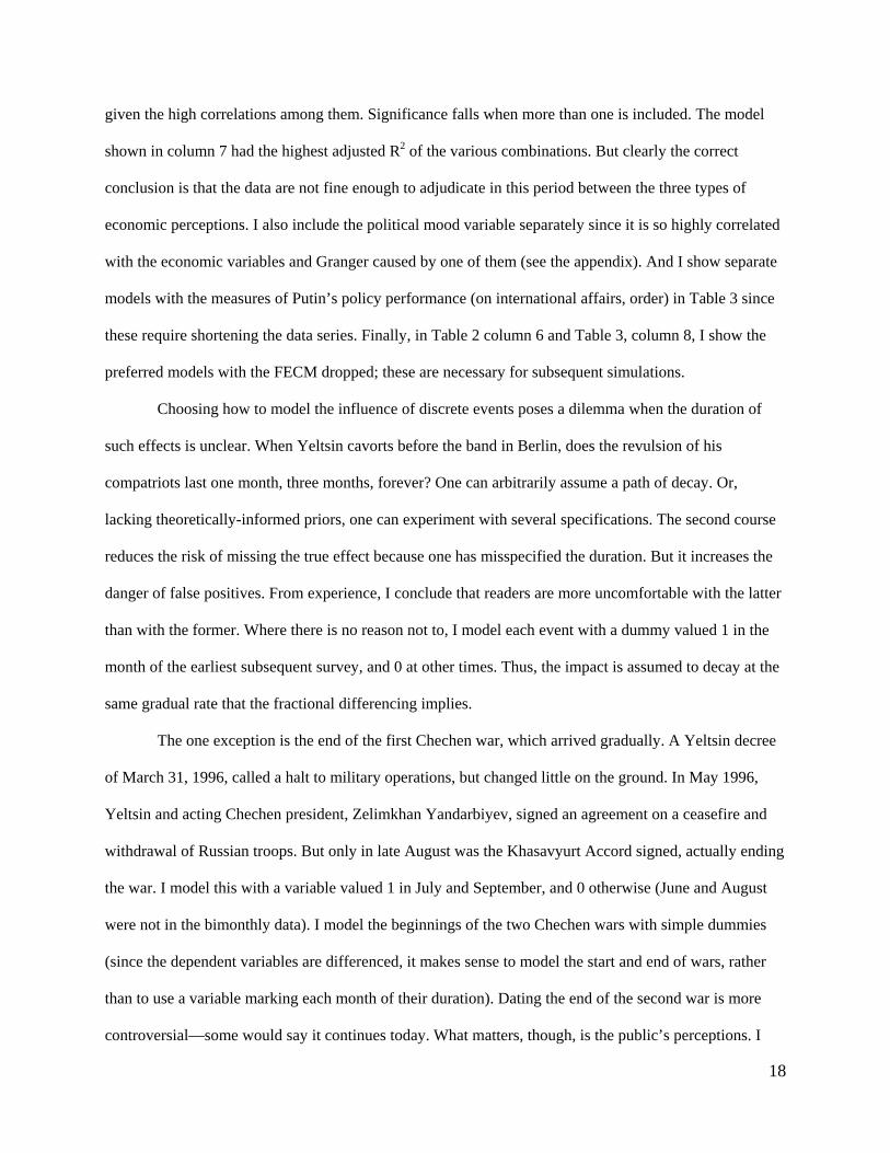
Table 3.  Explaining Putin’s popularity, Russia 2000‐2008                 Dependent variable is fractionally differenced percent approving of Putin’s performance (d = .646) 

  (1)  (2)  (3)  (4)  (5)  (6)  (7)  (8) 

d current economy  .29** (.12) 

        

  .17 (.15) 

.19 (.17) 

d family finances    .30** (.12) 

        .20 (.17) 

.22 (.17) 

d Russia’s ec. future      .16** (.07) 

         

d Political mood        .10 (.06) 

       

d Successful: International affairs 

        .19 (.14) 

     

d Successful: order            .15 (.21) 

   

d  “War continuing”  in Chechnya 

‐19.05 (16.68) 

‐40.99*** (12.19) 

‐26.56* (14.73) 

‐31.84** (13.75) 

‐21.09 (17.69) 

‐25.11 (18.13) 

‐29.61** (14.36) 

‐15.84 (25.32) 

d ECM(t‐1)  ‐.55*** (.09) 

‐.52*** (.10) 

‐.55*** (.10) 

‐.58*** (.10) 

‐.21 (.15) 

‐.52*** (.12) 

‐.54*** (.08) 

 

Months in office            

  ‐.04* (.02) 

‐.09*** (.03) 

Nordost theater siege   7.55*** (1.13) 

4.85*** (1.39) 

8.98*** (1.67) 

8.87*** (2.06) 

4.02* (2.05) 

6.53*** (1.27) 

6.71*** (1.39) 

4.31*** (1.31) 

Beslan terrorist attack  ‐.85 (1.25) 

‐.30 (1.32) 

‐.34 (1.38) 

2.88 (2.96) 

‐1.38 (1.28) 

‐.85 (1.38) 

   

Sinking of Kursk   ‐.46 (1.12) 

‐.17 (1.17) 

‐.60 (1.25) 

‐.65 (1.49) 

‐3.70* (2.10) 

‐1.42 (2.40) 

   

Soviet anthem restored  

6.88*** (.90) 

6.49*** (1.08) 

6.15*** (.90) 

7.73*** (1.05) 

8.95*** (1.32) 

6.84*** (1.41) 

6.32*** (.95) 

5.63*** (1.42) 

Nine eleven   ‐1.44 (1.25) 

‐.61 (1.22) 

‐.80 (.98) 

.10 (.93) 

‐.49 (1.71) 

.12 (1.24) 

‐1.34 (1.16) 

‐2.67* (1.56) 

Iraq war   ‐4.41*** (.79) 

‐3.41*** (.94) 

‐4.80*** (.72) 

‐4.88*** (.77) 

‐5.05*** (.74) 

‐5.90*** (1.89) 

‐3.84*** (.96) 

‐5.19*** (1.09) 

FH press index (high: less free) 

‐.14 (.10) 

‐.24** (.11) 

‐.16 (.11) 

‐.17 (.10) 

‐.33** (.15) 

‐.23 (.17) 

   

Takeover of NTV  ‐1.07 (1.00) 

‐1.67 (1.17) 

‐1.43 (1.03) 

‐.92 (1.10) 

‐4.40* (2.43) 

‐1.47 (1.18) 

   

Arrest of Khodorkovsky  

4.74*** (.96) 

4.58*** (.90) 

3.87*** (.84) 

3.87*** (.89) 

3.37* (1.72) 

5.24*** (1.49) 

4.74*** (.86) 

5.98*** (.82) 

L1 d rating  .26*** 

(.03) .28*** (.03) 

.22*** (.03) 

.28*** (.03) 

  

.34** (.15) 

.25*** (.03) 

 

Constant  12.45* (6.94) 

19.40** (7.84) 

13.92* (7.48) 

13.98* (7.19) 

24.71** (10.45) 

17.88 (11.80) 

5.18*** (1.44) 

9.02*** (1.59) 

R2  .6583  .6660  .6557  .6293  .5186  .5650  .6780  .4135 

LM  Autocorrelation test, χ2 

.18,  p =.67 

.67,  p =.41 

.06,  p =.80 

.02,  p =.89 

.11,  p =.74 

.11,  p = .74 

1.15,  p =.28 

.01, p =.91 

KPSS test of I(0)  .21, p < 1  .16, p < 1  .22, p < 1  .20, p < 1  .15, p < 1  .15, p <1  .14, p < 1  .27, p < 1 Durbin Watson statistic  2.09  2.18  1.94  1.96  1.91  2.06  2.20  1.84 N  49  49  49  49  40  41  49  49 *** p < .01, ** p < .05, * p < .10. OLS with robust standard errors in parentheses. Data bimonthly, starting in early 2000 and ending in February 

2008. d

series fractionally differenced using d estimated in Table A1.  ( 1)d

ECM t  is the fractionally differenced residuals from a 

regression of Putin’s approval on expected performance of the national economy (both in levels), lagged one two‐month period. Preferred model in bold.  

22

What do the results show? Consider first the effects of war and terrorist attacks. Yeltsin’s

Chechen misadventure does appear to have cost him support, although perhaps less than might have been

expected. His rating fell with the start of the first Chechen war, by a little less than one third of a point on

the 10 point scale (Table 2, column 5).38 It rose as the war ended in the summer of 1996. The regressions

suggest that the popularity gain from ending the war—a boost of a little less than one third of a point in

both the months of July and September—was larger than the popularity loss at the beginning, although of

course the estimates should be viewed as only approximate.39 The1995 terrorist siege of the hospital in

Budyonnovsk was followed by a drop in Yeltsin’s approval of about one quarter point. By contrast, the

start of the second Chechen war had no clear effect on the popularity of the departing Yeltsin.

Contrary to some conventional wisdom that links Putin’s appeal to Chechnya, the second war

seems to have weighed on his rating rather than boosting it. These regressions start in early 2000, and so

do not include Putin’s period as prime minister in 1999, during which his tough response to Basayev’s

invasion of Dagestan and the apartment explosions may indeed have bought him popularity (I discuss this

below). But after Putin’s election in March 2000, support for the war fell. In fact, his rating benefited in

2006-7 as Russians discerned some stabilization in Chechnya under the brutal leadership of Ramzan

Kadyrov. As the number saying that “peace was being established” in Chechnya rose, so too did Putin’s

rating. The “Nordost” terrorist seizure of a Moscow theater in 2002 led to a rally of about seven

percentage points for Putin. The Beslan attack of 2004, however, had no clear effect.

I lacked good data to assess the influence of presidential style conclusively. But it probably made

some difference. After Yeltsin’s stint conducting the band in Berlin, his rating fell by about one quarter

38 The fact that the dependent variable is fractionally differenced makes it harder to interpret the size of the effects. To get a sense of what difference this makes, I ran versions of the preferred models replacing the fractionally differenced dependent variable with the variable’s first difference. In almost all cases, the coefficients were similar, sometimes a little above and sometimes a little below the values in the tables. (The few exceptions concerned variables that were not statistically significant.) Thus, it is probably safe to assume that the size of the effects on presidential ratings are roughly those suggested by the coefficients in Tables 2 and 3. 39 And it is hard to think of anything else that a dummy for July and September 1996 could be picking up. These were months in which many Russians were experiencing buyer’s remorse, having reelected Yeltsin on July 3, only to discover he had secretly suffered a heart attack between the election rounds and needed quintuple bypass surgery, which he received in November.

23

point. I found no evidence, however, that Yeltsin’s hospitalizations affected his popularity. Perhaps his

ill-health was so well-known that hospitalization revealed little. As for Putin, his approval may have

fallen after the Kursk sank, but by a minuscule amount, not usually statistically significant. Restoring the

Soviet music to the national anthem produced a boost of around six points. It could be that this was the

moment Putin “closed the deal” with some former Communist supporters. Perhaps for the same reason,

the arrest of the oligarch Khodorkovsky led to a bounce of four or five points for Putin.

Respondents’ assessments of the prevailing political mood were not significant determinants of

popularity for either president. Evaluations of Putin’s success at establishing “order” in the country were

not significant, although this might merely reflect the data problems. I also found little evidence that

Putin’s international role influenced his rating. The percentage praising Putin’s international actions was

not significant and the estimated effect on his rating was small, although, again, the imperfect data might

be to blame. The 2003 US invasion of Iraq was followed by a drop in Putin’s approval of several points—

this extremely unpopular brandishing of American military power must have cast Putin’s previous

solicitousness towards the US after 9/11 in a bad light. The 9/11 terrorist attack and Putin’s quick support

for the US did not have a statistically significant effect. Nor was there a robust effect of the NATO

bombing of Kosovo, under President Yeltsin. As with US presidents, Yeltsin’s popularity did fall over

time, even controlling for other variables. Each month the downward pressure increased by .005 points,

adding up to about a half point by the end of his eight years in office. Putin’s approval may also have

fallen over time controlling for other effects.

What about the Kremlin’s growing control over the national press? The data on this—admittedly

limited—provide no evidence that Putin’s rating rose because of the Kremlin’s press mangement. His

rating was not improved by the takeover of NTV; the dummy for this was insignificant but negative. Nor

did greater media restrictions, as measured by Freedom House, bolster Putin’s image; in fact, the index’s

negative coefficient suggests his popularity fell as the state’s grip over the press tightened. (In any case,

the press freedom index was less significant in controlled regressions than tenure in office, with which it

was extremely highly correlated, so it drops out in the final regression.)

24

These results include a mixture of surprises and confirmations of the conventional wisdom.

Some of the factors discussed so far can help account for the jagged spikes in the ratings at various points.

But most of the effects are relatively small. By contrast, economic perceptions turn out to have

considerable explanatory power.40

Although the individual effects of the economic variables are hard to disentangle, their aggregate

impact is impressive. Under Yeltsin, the strongest effects were with perceptions of the national economy.

The FECM in columns 1 and 5, constructed using residuals from a regression of Yeltsin’s rating on

perceptions of the national economy, is significant, suggesting a long run relationship between positive

views of current conditions and support for the president. The coefficient’s value, -.23 in column 5,

implies that when a shock knocks the two variables out of equilbrium, about one quarter of the gap is

eliminated in each two-month period. The significant coefficients on the fractionally differenced current

economic perceptions measure suggest that such perceptions also had a short-term effect. Expectations

about future economic performance were significant when entered alone, but lost significance to current

economic perceptions if the two were included together. As one might expect, the 1998 financial crisis

depressed Yeltsin’s popularity, at least in regressions that do not control for perceptions of the national

economy; however reactions to the crisis were absorbed by such perceptions in column 1.

Under Putin, the evidence suggests a long run equilibrium relationship between economic

expectations and presidential approval—and the speed of re-equilibriation appears to have been relatively

fast: the coefficient of around .5 suggests that after a shock about half of the divergence was eliminated in

each two-month period. There is also evidence of short run effects, although the high mutual correlations

among economic variables makes it hard to say which matters more. Each of the three is significant if

entered alone (columns 1-3). But statistical significance falls if more than one is included at one time.

Since interpreting the coefficients on fractionally differenced variables is not straightforward, one

40 For instance, a model including all the variables in Table 2 except the economic ones has an adjusted R2 of .3913. Adding fractionally differenced current economy and family finances along with the FECM, the adjusted R2 jumps to .7290. Similarly, a model including all varaiables in Table 3 except the economic ones (I also leave out order and international affairs to avoid having to drop 8-9 observations) has an adjusted R2 of .2814. Adding fractionally differenced current economy and family finances along with the FECM, the adjusted R2 is .5227.

25

can get a sense of the size of the effects by simulating the path of presidential popularity holding

particular factors constant. How would Putin’s rating have changed, for instance, had he failed to produce

apparent progress towards stabilizing Chechnya? Using model 8, I simulated what Putin’s approval would

have been had the share of respondents who thought “war was continuing” in Chechnya remained at 100

percent rather than falling to 33 percent in late 2007. In this scenario, Putin’s rating would have dropped

from 79 percent in early 2000 to 56 percent later that year, before recovering to 72 percent in late 2007

(his actual rating at that point was 84 percent). What if Russians’ perceptions of the national economy and

of their family finances had remained frozen at December 1999 levels rather than improving under Putin?

Simulations suggest that his rating would have fallen from 79 percent to 59 percent in late 2007.

Of course, the economy had already begun to recover by early 2000 when Putin took office. The

odds are his popularity would have fallen still further had he presided over economic conditions as awful

as those under Yeltsin. Somewhat speculatively, one can explore this by simulating the model estimated

for Putin’s presidency (Table 3, column 8) but using the economic perceptions data not from Putin’s term

but from the corresponding months in Yeltsin’s, while leaving all other variables at their actual Putin-

presidency levels. Similarly, one can simulate what Yeltsin’s popularity might have been had perceived

economic conditions been those experienced under Putin (that is, I run the model from Table 2, column 6,

substituting the economic perceptions variables from the corresponding months in Putin’s term and

leaving all else as before). The two presidents’ simulated approval trajectories supposing they had

presided over the other’s perceived economic conditions are shown in Figure 2, panels a and b.41

This exercise should be taken with a grain of salt. The simulations change somewhat depending

on the model’s specification, and it was not possible to include an FECM.42 But the results are

nevertheless suggestive. It appears that Russians’ radically different evaluations of their first two

41 To simulate Putin with Yeltsin’s economy, it was necessary to impute values for economic perceptions under Yeltsin in 1992. To do this, I regressed the economic perceptions variables on inflation and real wages during the period when both were available and used the resulting models to impute backwards to 1992. 42 The dependent variable and residuals, from which the FECM is created, would themselves need to be the result of the simulation. This would require iterating at each period, estimating the dependent variable, computing the

26

presidents were heavily influenced by the very different economic conditions under which each served.

residual from the cointegrating regression, fractionally differencing it, and adding this to the error correction mechanism before estimating the dependent variable for the next period. Since without the full series of residuals, one could not know the appropriate d to fractionally difference them by, it is not clear how this could be done.

0

1

2

3

4

5

6

7

8

9

10

1991 1992 1993 1994 1995 1996 1997 1998 1999

Figure 2a.  What if perceived economic conditions under Yeltsin had been the same as under Putin? 

Simulated Yeltsin rating on 10‐point scale, supposing economic perceptions were same as in corresponding month under Putin

Yeltsin's actual rating

Source: VCIOM and author's calculations. 

0

10

20

30

40

50

60

70

80

90

100

2000 2001 2002 2003 2004 2005 2006 2007 2008

Figure 2b.  What if perceived economic conditions under Putin had been the same as under Yeltsin? 

Putin's actual approval

Simulated Putin approval supposing economic perceptions were same as in corresponding month under Yeltsin

Source: VCIOM/Levada Center and author's calculations

27

Had he presided over Putin’s economy, Yeltsin would likely have left office extremely popular. Had

Putin presided over Yeltsin’s economy, his rating would have fallen sharply early in his term, recovered

somewhat, but then dropped again towards the end. He would have left office with fewer than 50 percent

of Russians approving of his performance.43

The regressions also enable us to explore an intriguing counterfactual about Putin’s path to

power, which is usually seen as inexorably tied to the violent events of late 1999. Suppose there had been

no apartment bombings, no second Chechen war. Would Putin’s rating have remained around its starting

point of 31 percent, or slipped even lower? Were the traumas of late 1999 necessary to produce the rally

that took him to the Kremlin? Of course, we cannot know for sure. But the statistics offer some clues. To

see what economic perceptions alone would predict, I use the estimated effects of just economic

perceptions and months in office from Table 2, model 6, and simply extrapolate forward using the actual

economic perceptions data for the Putin presidency and restarting the months-in-office clock. I assume

the new president inherited Yeltsin’s dismal rating. In Figure 4, the dotted line shows the simulated rating

of a generic new president, based on just the dramatic economic improvement then occurring, supposing

that Russians started evaluating the new incumbent in September 1999, right after Putin took over as

prime minister (and Kremlin-endorsed presidential candiate). The dashed line supposes that Russians

started evaluating Putin in January 2000, as he took office as acting president. 44

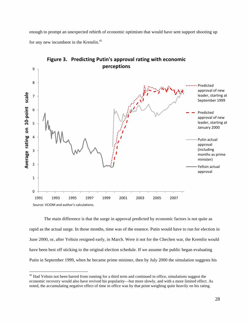
The striking implication of Figure 3 is that even without a Chechen war or terrorist attacks,

economic factors alone would have predicted a sharp jump in the new president’s popularity quite similar

to that which actually occurred. In late 1999, the Russian economy began to revive. Between August 1999

and June 2000, real wages rose by about 20 percent, while wage arrears and unemployment fell. This was 43 In fact, this probably underestimates Putin’s decline. For one thing, the simulations, which do not include the FECM, are thus unable to take into account the long run effect of the sharp drop in economic expectations under Yeltsin (in the Putin model, economic expectations are cointegrated with approval). Some, but probably not all, of this effect is captured by the coefficients on the short-run economic variables, which are slightly higher in column 8. 44 To be clear, no actual data on Putin’s approval were used in calculating this. Starting from the actual Yeltsin rating, I ran the model forward to produce predictions for each subsequent period, using the actual economic perceptions data, and restarting months-in-office. I am, therefore, assuming nothing about Yeltsin’s successor other than that he took office in either September 1999 (dotted line) or January 2000 (dashed line), inherited Yeltsin’s low initial popularity, and benefited from economic perceptions in the same way as Yeltsin had.

28

enough to prompt an unexpected rebirth of economic optimism that would have sent support shooting up

for any new incumbent in the Kremlin.45

The main difference is that the surge in approval predicted by economic factors is not quite as

rapid as the actual surge. In those months, time was of the essence. Putin would have to run for election in

June 2000, or, after Yeltsin resigned early, in March. Were it not for the Chechen war, the Kremlin would

have been best off sticking to the original election schedule. If we assume the public began evaluating

Putin in September 1999, when he became prime minister, then by July 2000 the simulation suggests his

45 Had Yeltsin not been barred from running for a third term and continued in office, simulations suggest the economic recovery would also have revived his popularity—but more slowly, and with a more limited effect. As noted, the accumulating negative effect of time in office was by that point weighing quite heavily on his rating.

0

1

2

3

4

5

6

7

8

9

1991 1993 1995 1997 1999 2001 2003 2005 2007

Average  rating  on  10‐point   scale

Figure 3.   Predicting Putin's approval rating with economic perceptions

Predicted approval of new leader, starting at September 1999

Predicted approval of new leader, starting at January 2000

Putin actual approval (including months as prime minister)

Yeltsin actual approval

Source: VCIOM and author's calculations. 

29

rating would have reached 4.5 on the 10-point scale. If we suppose instead that Putin’s initial approval in

January 2000 was anchored to Yeltsin’s final November 1999 score, his simulated rating by July would

have been 3.8. Yeltsin’s rating when he won reelection in July 1996, with 54 percent of the valid vote,

had been 3.9. Thus, it is very possible that Putin—or some other generic new Kremlin candidate—would

have won the presidency without the effect of the Chechen conflict and terrorist bombings.

However, economic factors do not explain why Putin’s rating actually surged when it did. This

might, indeed, be associated with the Chechen events. To examine this further, I experimented with

regressions going back to September 1999, combining Putin’s prime ministerial rating with his

presidential rating. A dummy variable for the months of September to November 1999 is statistically

significant, with a large coefficient. Something different—most likely the terrorist attacks and Chechen

events—caused a rallying behind Putin during these months that went beyond the powerful effects of

economic recovery. Although economic factors would have achieved the same result a few months later,

the traumas of late 1999 apparently sped things up.46

5 The determinants of economic perceptions

The importance of economic perceptions raises the question: what caused these perceptions? Did they

reflect actual economic conditions, were they idiosyncratic, or were they manipulated by government

public relations? It might seem that Russians’ rosy view of the economy under Putin was itself a result of

the Kremlin’s growing dominance over national television. Or a sanguine view of the economy might

reflect a general feeling of confidence in the regime and in Putin’s stewardship.

To explore this, I ran fractional error correction models with the fractionally differenced

economic perceptions measures as the dependent variables (Table 4). Among the explanatory

variables, I included six objective measures of economic conditions—the average real wage, the real

46 This very positive effect of Chechnya in late 1999 contrasts with the longer term reaction to the war, which, as noted, apparently decreased enthusiasm for Putin (Table 3). It seems that the sense of external attack prompted an intense rally behind the leadership, but that over time, as other opinion polls suggest, support for military operations fell and Russians switched to rewarding the president for moves towards stabilization.

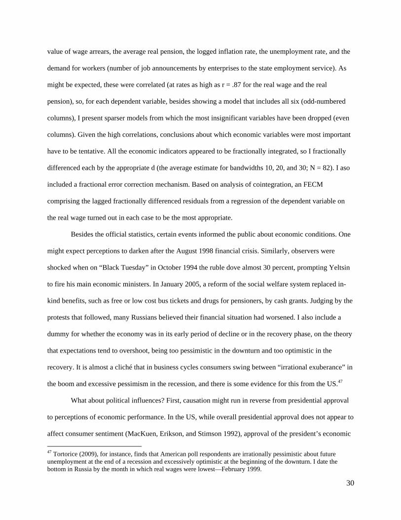
30

value of wage arrears, the average real pension, the logged inflation rate, the unemployment rate, and the

demand for workers (number of job announcements by enterprises to the state employment service). As

might be expected, these were correlated (at rates as high as r = .87 for the real wage and the real

pension), so, for each dependent variable, besides showing a model that includes all six (odd-numbered

columns), I present sparser models from which the most insignificant variables have been dropped (even

columns). Given the high correlations, conclusions about which economic variables were most important

have to be tentative. All the economic indicators appeared to be fractionally integrated, so I fractionally

differenced each by the appropriate d (the average estimate for bandwidths 10, 20, and 30; N = 82). I aso

included a fractional error correction mechanism. Based on analysis of cointegration, an FECM

comprising the lagged fractionally differenced residuals from a regression of the dependent variable on

the real wage turned out in each case to be the most appropriate.

Besides the official statistics, certain events informed the public about economic conditions. One

might expect perceptions to darken after the August 1998 financial crisis. Similarly, observers were

shocked when on “Black Tuesday” in October 1994 the ruble dove almost 30 percent, prompting Yeltsin

to fire his main economic ministers. In January 2005, a reform of the social welfare system replaced in-

kind benefits, such as free or low cost bus tickets and drugs for pensioners, by cash grants. Judging by the

protests that followed, many Russians believed their financial situation had worsened. I also include a

dummy for whether the economy was in its early period of decline or in the recovery phase, on the theory

that expectations tend to overshoot, being too pessimistic in the downturn and too optimistic in the

recovery. It is almost a cliché that in business cycles consumers swing between “irrational exuberance” in

the boom and excessive pessimism in the recession, and there is some evidence for this from the US.47

What about political influences? First, causation might run in reverse from presidential approval

to perceptions of economic performance. In the US, while overall presidential approval does not appear to

affect consumer sentiment (MacKuen, Erikson, and Stimson 1992), approval of the president’s economic

47 Tortorice (2009), for instance, finds that American poll respondents are irrationally pessimistic about future unemployment at the end of a recession and excessively optimistic at the beginning of the downturn. I date the bottom in Russia by the month in which real wages were lowest—February 1999.

31

management does (De Boef and Kellstedt 2004). Given the evidence already presented that economic

perceptions affect presidential approval, we should expect the two to be correlated. So in estimating the

impact of economic indicators on economic perceptions, one should at least control for presidential

approval. In the regressions, I include the differenced rating of the incumbent on the 10-point scale. (My

estimate of the order of integration was almost exactly 1, so first differencing was appropriate.)

Certain government actions are likely to influence economic perceptions. I included a dummy for

Khodorkovsky’s arrest to see whether the prosecution of the country’s leading businessman was viewed

as good or bad for the economy (recall that Putin’s approval jumped). Finally, officials manipulate media

coverage of the economy. I included a dummy for Putin’s presidency to test the common presumption

that coverage became more favorable under him. I also tried including Freedom House’s index of press

freedom, which I used in the regressions for Putin era presidential approval. Media effects are expected to

be particularly strong during election campaigns. I included variables valued 1 for the six months before a

presidential election and -1for the six months after it.48

The first point to note about the results in Table 4 is that the public’s view of economic conditions

is not just idiosyncratic. Each of the perceptions variables is systematically related to objective measures

of economic performance. All three appear to be in long run equilibrium with the average real wage. The

coefficients on the FECM are significant and suggest that when the real wage increases economic

perceptions adjust upward to a new equilbrium; between a quarter and a third of the gap is closed each

two-month period.49 In the short run, more job vacancies and, possibly, lower wage arrears (not

significant) were associated with a more positive view of the current economy. Short run increases in

wages and pensions and decreases in unemployment correlated with a rosier view of family finances.

Rising pensions, falling wage arrears, and, perhaps, falling unemployment (not significant) were

associated with more sanguine expectations. Inflation was never significant, perhaps because its effects

48 For a similar approach, see De Boef and Kellstedt (2004). 49 The real driver might, of course, be some other economic indicator correlated with the real wage. However, results were most significant using it in the FECM.

32

Table 4.  Determinants of economic perceptions Dependent variable d current economy (d = .947)

d family finances (d = .505) d Russia’s ec. future (d = .884)

  (1)  (2) (3) (4) (5)  (6)

Economic data             

     d real wage  .003 

(.015)   .004 

(.012) .011* (.007) 

.007 (.020) 

 

     d real wage arrears  ‐.045 

(.038) ‐.044 (.026) 

.069 (.059) 

  ‐.12** (.05) 

‐.11** (.05) 

     d unemployment  .25 

(1.24)   ‐1.81 

(1.44) ‐2.03* (1.17) 

‐2.91 (2.40) 

‐2.76 (1.83) 

     d log inflation  2.61 

(3.52)   1.67 

(3.63)   3.06 

(7.40)  

     d demand for workers  .009 

(.006) .009** (.004) 

.001 (.005) 

  ‐.00 (.01) 

 

     d average real pension  .023 

(.027)   .050** 

(.025) .057*** (.019) 

.10* (.05) 

.094*** (.035) 

     d ECM(t‐1)  ‐.28*** 

(.09) ‐.31*** (.09) 

‐.36*** (.09) 

‐.34*** (.08) 

‐.27* (.15) 

‐.27** (.12) 

     Recovery phase  2.81 (2.00) 

1.81** (.88) 

9.28*** (2.30) 

8.11*** (1.73) 

1.17 (4.54) 

 

Economic events                  1998 financial crisis   

‐16.42*** (4.90) 

‐16.39*** (2.82) 

‐.22 (7.16) 

  ‐2.94 (7.60) 

 

     Oct. 1994 financial crisis  ‐5.07 (3.08) 

‐5.37*** (1.17) 

‐.02 (2.66) 

  ‐11.73** (5.39) 

‐12.47*** (1.28) 

     Monetization of benefits,       Jan 2005 

‐1.78 (1.33) 

‐1.04 (.68) 

‐15.75*** (2.09) 

‐15.38*** (1.60) 

‐5.89* (3.06) 

‐5.42** (2.05) 

Politics                  Putin presidency dummy  ‐2.26 

(2.02)   ‐5.72** 

(2.59) ‐5.17*** (1.72) 

‐3.59 (4.69) 

 

      President’s rating       (10 point scale) 

3.57*** (1.26) 

2.90*** (1.06) 

1.85** (.76) 

1.15** (.47) 

7.23*** (1.71) 

6.91*** (1.69) 

     Khodorkovsky arrested  

‐5.82*** (1.73) 

‐5.37*** (1.17) 

.64 (1.99) 

  ‐6.23** (2.80) 

‐6.11*** (2.15) 

     Press freedom       (high = less free) 

.07 (.11) 

  ‐.03 (.08) 

  .10 (.17) 

 

     1996 campaign  3.07* (1.53) 

3.50*** (1.22) 

‐1.14 (1.38) 

‐1.57* (.90) 

3.56 (2.15) 

3.86** (1.93) 

     2000 campaign  ‐2.27 (2.58) 

  ‐1.66 (2.12) 

  6.16 (7.19) 

6.94 (7.15) 

     2004 campaign  4.46*** (1.22) 

4.50*** (1.02) 

‐.33 (.91) 

  8.53*** (1.70) 

8.79*** (1.54) 

     2008 campaign  ‐.49 (2.02) 

  ‐2.88* (1.65) 

‐3.28*** (.68) 

‐5.90** (2.33) 

‐4.30*** (.94) 

Constant  ‐4.39 (5.74) 

‐.75 (.70) 

‐1.01 (4.33) 

‐2.55*** (.69) 

‐4.77 (8.75) 

.31 (.73) 

R2  .5429  .5193  .6490  .6197  .5128  .5038 

LM  Autocorrelation test, χ2 (p)  .59 (.44)  .86 (.35)  .06 (.81)  1.41 (.24)  .19 (.67)  .20, p = .66 KPSS test of I(0)  .03, p < 1  .03, p < 1  .03, p < 1  .04, p < 1  .05, p < 1  .10, p < 1 Durbin Watson statistic  2.10  2.10  2.03  2.16  2.08  2.09 N  81  81  81  81  80  80 *** p < .01, ** p < .05, * p < .10. OLS with robust standard errors in parentheses. Data are bimonthly, starting in early 1994, when contiuous 

bimonthly economic series begin, ending in December 2007. d

:  series fractionally differenced using estimated d (average for bandwidths of 

30, 20, and 10). d

 President’s rating: on 10‐point scale. 

d ECM(t‐1) is fractionally differenced one period lag of residuals of regression of 

dependent variable on real wage (both in levels). Even columns show models from which the most insignifiant variables have been dropped.  

33

were captured here by change in the real wage and pension. The regressions also support the hypothesis

that attitudes overshoot, accentuating the current trend; even controlling for political factors, views of the

current economy and of family finances were more negative during the downslide and positive during the

recovery than would be predicted by just the objective economic indicators.

As expected, major economic events also triggered reevaluations. The 1998 financial crisis

lowered assessments of the current economy dramatically, although surprisingly it did not influence

expectations. Both evaluations of the current economy and economic expectations sank after the October

1994 currency crisis. If these events hit Russians in the pocketbook, the effect was captured by economic

indicators included in the regressions. By contrast, the monetization of benefits in January 2005 prompted

a sharp fall in how well-off many Russians felt, and also led to more pessimistic expectations.

The extent to which objective economic indicators and events can account by themselves for the

pattern of economic perceptions can be seen in Figures 4a and 4b. The dashed lines represent values

predicted using just the economic variables in models 2 and 4 of Table 4. (That is, I use the coefficients

on economic variables in columns 2 and 4 to predict the fractionally differenced dependent variable,

leaving out the political effects, and convert the predictions to levels.) These predictions do not catch all

the spikes and dives in the perceptions series. But they do an excellent job of capturing the trends.

Politics helps explain the remaining variation. Presidential approval was, as expected, correlated

with all three economic perceptions measures; controlling for it allows greater confidence in the estimated

impact of the economic variables. The coefficients on presidential approval—2.90, 1.15, and 6.91, in

columns 2, 4, and 6—provide estimates of the extent of reverse causation. For the current economy and

family finances, such effects seem minor. Of the 84-point range of the current economy variable,

presidential popularity could predict about 16 points, and it could predict about six points of the 77-point

range in family finances.50 The possible effect of presidential approval on economic expectations is

50 The range of the presidential rating was 5.6 points. Multiplying this by the estimated coefficients on current economy and family finances yields 16.2 points for current economy and 6.4 points for family finances.

34

somewhat larger—the former could predict up to 39 points in the 81-point range of the latter.51

  

 

51 To disentangle the relationships further is difficult since they appear to be simultaneous. Attempts at causal modeling using lagged fractional differences of independent variables turned up no statistically significant results.

‐100

‐90

‐80

‐70

‐60

‐50

‐40

‐30

‐20

‐10

0

1994 1995 1996 1997 1998 1999 2000 2001 2002 2003 2004 2005 2006 2007

Figure 4a.   Perceptions of the national economy and their economic determinants

Russians' assessment of current national economy

Assessment of national economy predicted from just economic variables

‐90

‐80

‐70

‐60

‐50

‐40

‐30

‐20

‐10

0

1994 1995 1996 1997 1998 1999 2000 2001 2002 2003 2004 2005 2006 2007

Figure 4b.   Perceptions of family finances and their economic determinants

Russians' assessment of their family finances

Assessment of family finance predicted from just economic variables

Source: VCIOM and author's calculations. 

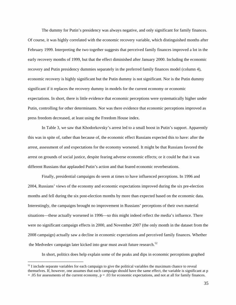
35

The dummy for Putin’s presidency was always negative, and only significant for family finances.

Of course, it was highly correlated with the economic recovery variable, which distinguished months after

February 1999. Interpreting the two together suggests that perceived family finances improved a lot in the

early recovery months of 1999, but that the effect diminished after January 2000. Including the economic

recovery and Putin presidency dummies separately in the preferred family finances model (column 4),

economic recovery is highly significant but the Putin dummy is not significant. Nor is the Putin dummy

significant if it replaces the recovery dummy in models for the current economy or economic

expectations. In short, there is little evidence that economic perceptions were systematically higher under

Putin, controlling for other determinants. Nor was there evidence that economic perceptions improved as

press freedom decreased, at least using the Freedom House index.

In Table 3, we saw that Khodorkovsky’s arrest led to a small boost in Putin’s support. Apparently

this was in spite of, rather than because of, the economic effect Russians expected this to have: after the

arrest, assessment of and expectations for the economy worsened. It might be that Russians favored the

arrest on grounds of social justice, despite fearing adverse economic effects; or it could be that it was

different Russians that applauded Putin’s action and that feared economic reverberations.

Finally, presidential campaigns do seem at times to have influenced perceptions. In 1996 and

2004, Russians’ views of the economy and economic expectations improved during the six pre-election

months and fell during the six post-election months by more than expected based on the economic data.

Interestingly, the campaigns brought no improvement in Russians’ perceptions of their own material

situations—these actually worsened in 1996—so this might indeed reflect the media’s influence. There

were no significant campaign effects in 2000, and November 2007 (the only month in the dataset from the

2008 campaign) actually saw a decline in economic expectations and perceived family finances. Whether

the Medvedev campaign later kicked into gear must await future research.52

In short, politics does help explain some of the peaks and dips in economic perceptions graphed

52 I include separate variables for each campaign to give the political variables the maximum chance to reveal themselves. If, however, one assumes that each campaign should have the same effect, the variable is significant at p = .05 for assessments of the current economy, p = .03 for economic expectations, and not at all for family finances.

36

in Figure 4. Russians’ greater approval of Putin than of Yeltsin may have fed back, exacerbating

economic pessimism in the late Yeltsin period and fueling optimism in the early Putin years. Biased

media might help to explain the surges and subsequent falls of economic optimism during the presidential

campaigns of 1996 and 2004. On the other hand, I found no evidence of systematically greater distortions

under Putin than under Yeltsin. Overall, the trends in economic perceptions were well predicted by just

the economic indicators. Perceptions of the economy tanked under Yeltsin and soared under Putin not

because of effective propaganda but because the underlying economic variables were doing the same.

6 Conclusion

From Argentina to Poland, politics in young democracies is a game full of surprises. Politicians’ ratings

wax and wane, sometimes very rapidly. Electorates swing between candidates and parties, at times

embracing complete unknowns. It is easy to attribute such volatility to an unhealthy brew of rootless

voters, demagogic politicians, and media manipulation. However, in some cases it may have quite a

different cause: electoral volatility may reflect underlying economic volatility—and the efforts of rational

voters, even in difficult circumstances, to hold their leaders to account.

In Russia, presidential ratings since 1991 have traced a pattern of dramatic slides and sudden

leaps. The collapse of Yeltsin’s popularity and the soaring support for Putin are often linked to their

personalities and public images.53 Others see in Putin’s ratings an endorsement of his Chechen military

campaign and ambitions to rebuild the Russian state (Sil and Chen 2004). Still others suppose that

Russians backed Putin because they had been brainwashed by a state-controlled media from which

criticism of the Kremlin had been eliminated (Ryzhkov 2004).

Wartime rallies, media effects, and image did play a part at times. Perhaps were better data

available their role would turn out to be somewhat greater. However, the evidence suggests that Russians’

53 Anderson (2007), for instance, attributes Putin’s popularity largely to his “image of firm, where necessary ruthless authority,” and claims to see a link to Russian culture: “Historically, the brutal imposition of order has been more often admired than feared in Russia… In what remains in many ways a macho society, toughness–prowess in judo and drops into criminal slang are part of Putin’s kit–continues to be valued.”

37

perceptions of economic conditions have been more consistently important. Much like citizens in Western

democracies, Russians approved of their president when they saw the economy improving and felt

hopeful about its future. Although government public relations influenced these perceptions, especially

during certain electoral campaigns, Russians’ views of the economy were closely related to objective

economic indicators, in particular the levels and recent changes in real wages, pensions, and wage arrears.

From this perspective, the political fates of Russia’s first two presidents appear in a new light.

Yeltsin’s ignominious slide in the public’s affections and Putin’s unprecedented eight years of adulation

appear to have been largely predetermined by the economic conditions each inherited. (Of course, each

influenced the economy on his watch; but it is hard to deny that Yeltsin inherited the decrepit Soviet

system in the middle of a macroeconomic disaster, whereas Putin benefited from a recovery fueled by

soaring world commodity prices.) Simulations suggest that a generic new president inaugurated in 2000

would have become extremely popular—whether or not he practiced judo—because of the boom.

The analysis also implies that, were income growth to falter for an extended period , this would

likely weigh on the approval of President Medvedev and now Prime Minister Putin. Judging by the

simulations, however, it could take a long time for even quite dramatic economic deterioration to drag

down the leaders’ ratings from their current extraordinary highs. The model could change—if, for

instance, civil disturbances fed on each other, and the regime responded in counter-productive and

provocative ways, catalyzing further decline. But should Russians continue to evaluate their incumbent

leaders as they have done in recent years, the fall should be gradual.

These conclusions fit with a body of recent work that has been discovering familiar rational

behavior beneath the paradoxical and irregular surface of political life in developing and middle income

countries (Drazen 2008). Outside the rich democracy club, information is unusually asymmetric,

uncertainty is endemic, and economic conditions often fluctuate wildly. In such environments, quite

rational behavior gives the impression of impulsiveness and manipulation. While miscalculations and

fraud are certainly common in transitional democracies, so too, it turns out, is retrospective voting. From

Peru to Poland, scholars have found that “governments are being held accountable for bad economic

38

policies, at least to some degree” (Lewis-Beck and Stegmaier 2008, p.320). The irony is that in such

countries economic conditions are particularly vulnerable to global forces, which complicates the task for

voters—regardless how sophisticated—of separating noise from signals about incumbent competence.

39

References

Anderson, Perry. 2007. “Russia’s Managed Democracy,” London Review of Books, 29, 2, pp.3-12. Arce, Moisés. 2003. “Political Violence and Presidential Approval in Peru,”Journal of Politics, 65, 2, May, pp. 572–583. Baum, Christopher and John Barkoulas. 2006. “Dynamics of Intra-EMS Interest Rate Linkages,” Journal of Money, Credit, and Banking, 38, 2, pp.469-82. Box-Steffensmeier, Janet M. and R.M. Smith. 1996. “The Dynamics of Aggregate Partisanship,” American Political Science Review, 90, pp.567-80. Box-Steffensmeier, Janet M. and Andrew R. Tomlinson. 2000. “Fractional integration methods in political science,” Electoral Studies, 19, pp.63-76. Box-Steffensmeier, Janet M., David Darmofal, and Christian A. Farrell. 2009. “The Aggregate Dynamics of Campaigns,” The Journal of Politics, 71, 1, 2009, pp. 309–323. Cheung, Y.-W., and K.S. Lai. 1993. A Fractional Cointegration Analysis of Purchasing Power Parity. Journal of Business and Economic Statistics 11, 103–112. Clarke, Harold D. and Matthew Lebo. 2003. “Fractional (Co)integration and Governing Party Support in Britain,” British Journal of Political Science, 33, pp.283-301. Clarke, Harold and Marianne C. Stewart. 1995. “Economic Evaluations, Prime Ministerial Approval and Governing Party Support: Rival Models Reconsidered,” British Journal of Political Science, 25, pp.145-70. Colton, Timothy J. 2000. Transitional Citizens: Voters and What Influences Them in the New Russia, Cambridge, MA: Harvard University Press. Colton, Timothy J. 2008. Yeltsin: A Life, New York: Basic Books. Colton, Timothy J. and Henry E. Hale. 2008. “The Putin Vote: The Demand Side of Hybrid Regime Politics,” George Washington University: unpublished. De Boef, Suzanna and Paul M. Kellstedt. 2004. “The Political (and Economic) Origins of Consumer Confidence,” American Journal of Political Science, 48, 4, pp.633-49. Dominguez, Jorge I., and James A. McCann. 1996. Democratizing Mexico: Public Opinion and Electoral Choices, Baltimore: Johns Hopkins University Press. Doukhan, Paul, Georges Oppenheim and Murad S. Taqqu, eds. 2003. Theory and Applications of Long-Range Dependence: Theory and Applications, Basel: Birkhäuser. Drazen, Allan. 2008. “Is There a Different Political Economy fro Developing Countries? Issues, Perspectives, and Methodology,” Journal of African Economies, 17, 1, pp.18-71. Duch, Raymond M. 1995. “Economic Chaos and the Fragility of Democratic Transitions in Former Communist Regimes.” Journal of Politics, 37, 1, pp. 121-58.

40

Duch, Raymond M. 2002. “A Developmental Model of Heterogeneous Economic Voting in New Democracies,” American Political Science Review, 95, 4, pp.895-910. Dueker, M., and R. Startz. 1998. Maximum-Likelihood Estimation of Fractional Cointegration with an Application to U.S. and Canadian Bond Rates. The Review of Economics and Statistics, pp.420–426. Erikson, Robert S., Michael B. MacKuen, and James A. Stimson. 2002. The Macro Polity, New York: Cambridge University Press. Haldrup, Niels and Morten Orregaard Nielsen. 2007. “Estimation of Fractional Integration in the Presence of Data Noise,” Computational Statistics & Data Analysis, 51, 6, pp.3100-3114. Hale, Henry. 2009. “The Myth of Mass Authoritarianism in Russia: Public Opinion Foundations of a Hybrid Regime,” George Washington University: manuscript. Hesli, Vicki L. and Elena Bashkirova. 2001. “The Impact of Time and Economic Circumstances on Popular Evaluations of Russia’s President,” International Political Science Review, 22, 4, pp.379-98. Jeffries, Ian. 2002. The New Russia: A Handbook, New York: Routledge. Lafay, J.D. 1991. “Political Dyarchy and Popularity Functions: Lessons from the 1986 French Experience,” in Norpoth, H., M. Lewis-Beck, and J.D. Lafay, Economics and Politics: The Calculus of Support, 1991, Ann Arbor: University of Michigan Press, pp.123-39. Lebo, Matthew J. and Daniel Cassino. 2007. “The Aggregated Consequences of Motivated Reasoning and the Dynamics of Partisan Presidential Approval,” Political Psychology, 28, 6, pp.719-46. Lewis-Beck, Michael, and Mary Stegmaier. 2008. “The Economic Vote in Transitional Democracies,” Journal of Elections, Public Opinion & Parties,18, 3, pp.303-23. MacKuen, Michael, B., Robert S. Erikson, and James A. Stimson. 1992. “Peasants or Bankers? The American Electorate and the US Economy,” American Political Science Review, 86, 3, pp.597-611. Mansfield, Edward D. and Jack Snyder. 1995. “Democratization and the Danger of War,” International Security, 20, 1, pp. 5-38. Miller, Arthur H., William Reisinger, and Vickie L. Hesli. 1996. “Understanding Political Change in Post-Soviet Societies: A Further Commentary on Finifter and Mickiewicz.” American Political Science Review, 90, 1, pp. 153-66. Mishler, William and John Willerton. 2003. “The Dynamics of Presidential Popularity in Post-Communist Russia: Cultural Imperative versus Neo-Institutional Choice?” Journal of Politics, 65, 1, pp.111-141.

Morin, Richard, and Nilanthi Samaranayake. 2006. The Putin Popularity Score: Increasingly Reviled in the West, Russia's Leader Enjoys Broad Support at Home, Washington, DC: Pew Research Center.

Mueller, John. 1973. War, Presidents, and Public Opinion, New York: Wiley. Remnick, David. 2007. “Letter from Moscow: The Tsar’s Opponent,” The New Yorker, October 1.

41

Robinson, P. M. 1995. “Gaussian semiparametric estimation of long range dependence,” Annals of Statistics, 23, pp.1630-61. Rogoff, Kenneth and Anne Sibert. 1988. “Elections and macroeconomic policy cycles,” Review of Economic Studies, 55, pp.1-16. Rose, Richard. 2007a. “Going Public with Private Opinions: Are Post-Communist Citizens Afraid to Say What They Think?” Journal of Elections, Public Opinion, and Parties, 17, 2, pp.123-42. Rose, Richard. 2007b. “The Impact of President Putin on Popular Support for Russia’s Regime,” Post-Soviet Affairs, 23, 3. Rose, Richard, William Mishler, and Neil Munro. 2004. “Resigned Acceptance of an Incomplete Democracy: Russia’s Political Equilibrium,” Post-Soviet Affairs, 20, 3, pp.195-218. Rzyhkov, Vladimir. 2004. “The Liberal Debacle,” Journal of Democracy, 15, 3, pp.52-8. Sanders, David. 2000. “The real economy and the perceived economy in popularity functions: how much do voters need to know? A study of British data, 1974-97,” Electoral Studies, 19, pp.275-94. Sil, Rudra and Cheng Chen. 2004. “State Legitimacy and the (In)significance of Democracy in Post-Communist Russia,” Europe-Asia Studies, 56, 3, pp. 347-368.

Tortorice, Daniel L. 2009. “Unemployment expectations and the business cycle,” Brandeis: manuscript. Tucker, Joshua A. 2006. Regional Economic Voting: Russia, Poland, Hungary, Slovakia and the Czech Republic, 1990-1999, New York: Cambridge University Press. Weyland, Kurt. 2003. “Economic Voting Reconsidered: Crisis and Charisma in the Election of Hugo Chávez,” Comparative Political Studies, 36,7, September, pp.822-848. White, Stephen and Ian Mcallister. 2008. “The Putin Phenomenon,” Journal of Communist Studies and Transition Politics, 24, 4, pp.604-28. White, Stephen, Sarah Oates, and Ian McAllister. 2005. “Media Effects and Russian Elections, 1999” British Journal of Political Science, 35, pp.191-208. Whitefield, Stephen. 2005. “Putin’s Popularity and Its Implications,” in Alex Pravda, ed., Leading Russia: Putin in Perspective, Essays in Honour of Archie Brown, New York: Oxford University Press, pp.139-160. Wyman, Matthew. 1997. Public Opinion in Postcommunist Russia, New York: St Martin’s Press. Yeltsin, Boris. 2000. Midnight Diaries, New York: Public Affairs.

42

Appendix A1. Distribution of evaluations of Yeltsin on 10-point scale

A2. Analyzing the relationship between economic perceptions and perceptions of the political situation I use causal modeling with fractionally differenced variables to examine the relationship between the

economic and political perceptions variables. Testing for Granger causality (1969) requires one to regress

a dependent variable on lags of itself and one or more possible explanatory variables. If the lagged

explanatory variables are statistically significant, one concludes that they “Granger cause” the dependent

variable. This method has been applied to fractionally differenced variables in, for instance, Box-

Steffensmeier, Darmofal and Farrell (2009).

From the estimates in Table A1 we can conclude that Russians’ expectations about future

economic performance probably Granger caused their evaluations of the political situation during the

Yeltsin period (this is significant at p = .08; second column). Evidence of causation running from

evaluations of the political system to expectations of future economic performance was less significant (p

Figure A1.a Distribution of evaluations of Yeltsin's performance, October 1991

0

5

10

15

20

1 2 3 4 5 6 7 8 9 10

Score on 10 point scale

Per

cen

t o

f va

lid r

esp

on

ses

Figure A1b. Distribution of evaluations of Yeltsin's performance, September 1999

0

10

20

30

40

50

60

70

80

1 2 3 4 5 6 7 8 9 10

Score on 10 point scale

Per

cen

t o

f va

lid r

esp

on

ses

43

= .15; fourth column). There was no evidence that economic perceptions affected political perceptions

during the Putin period, however.

  Table A1.  Economic and political perceptions: causal modeling 

                                                           ‐‐‐‐‐‐‐‐‐‐‐‐‐‐‐‐‐Yeltsin presidency‐‐‐‐‐‐‐‐‐‐‐‐‐‐‐‐‐                      ‐‐‐‐‐‐‐‐‐‐‐‐‐‐‐‐‐‐‐Putin presidency‐‐‐‐‐‐‐‐‐‐‐‐‐‐‐‐‐‐ 

  d  political situation 

d  political situation 

d   current economy 

d  Russia’s ec. future 

d  political situation 

d  political situation 

d   current economy 

d  Russia’s ec. future 

L1 d political situation  .24 

(.17) .45*** (.13) 

.00 (.12) 

.26 (.17) 

‐.19 (.13) 

‐.23 (.14) 

.01 (.06) 

‐.13 (.20) 

L1 d current economy  .29 

(.29)   .17 

(.19)   ‐.07 

(.31)   ‐.16 

(.18)  

L1 d Russia’s ec. future   

 .27* (.15) 

  .31* (.17) 

  .06 (.19) 

  .25 (.24) 

L2 d dependent var.  .30 

(.18)             .21 

(.18)                  Constant  ‐3.92** 

(1.53) ‐4.00** (1.49) 

‐.91 (1.57) 

‐.47 (3.01) 

5.13*** (1.61) 

4.96*** (1.65) 

   2.50*** (.70) 

2.07* (1.22) 

R2  .4061  .4761  .0262  .1778  .0423  .0437  .0223  .1235 

Durbin Watson  2.09  2.19  1.91  1.77  1.97       2.00  2.00  1.99 

LM autocorrelation test, χ2  

1.73,  p = .19 

.95 p =.33 

.22 p = .64 

.15 p =.70 

.23 p =.63 

1.19 p =.28 

.43 p =.51 

1.01 p =.32 

KPSS test of I(0)  .12 (p < 1)  .28 (p < 1)  .10 (p < 1)  .08 (p < 1)  .33 (p < 1)  .35 (p < 1)  .21 (p < 1)  .11 (p < 1) 

N  31  32  32  32  50  50  50  50 

*** p < .01, ** p < .05, * p < .10. OLS with robust standard errors in parentheses.d : series fractionally differenced using d 

estimated in Table 1; Lk: kth lag of the variable. Lags of the dependent variable were included when necessary to reduce autocorrelation.  

44

Table A2.   Variable definitions and data sources Variable  Definition  Source  

Yeltsin What evaluation from 1 (lowest) to 10 (highest) would you give the President of Russia Boris Yeltsin?  Mar 1994‐Nov 1999, bimonthly series.  

http://sofist.socpol.ru, http://www.levada.ru/programs.html, Ekonomicheskie i Sotsialnie peremeni: monitoring obshchestvennogo mnenia, various issues, Russiavotes.org 

Approval On the whole do you approve or disapprove of the performance of President ____? % saying they approve. Sep 1996‐Mar 2008.  

http://www.levada.ru/programs.html, Ekonomicheskie i Sotsialnie peremeni: monitoring obshchestvennogo mnenia, various issues, Russiavotes.org 

russec How would you assess Russia’s present economic situation?  Very good + good ‐ (Very bad + bad), %, there is also category "in between"; Mar 1994‐Mar 2008, bimonthly series. 

http://www.levada.ru/programs.html, Ekonomicheskie i Sotsialnie peremeni: monitoring obshchestvennogo mnenia, various issues, Russiavotes.org 

fammat How would you assess your family’s present material condition? Very good + good ‐ (Very bad + bad), %, there is also category "in between"; Mar 1994‐Mar 2008, bimonthly series. 

http://www.levada.ru/programs.html, Ekonomicheskie i Sotsialnie peremeni: monitoring obshchestvennogo mnenia, various issues, Russiavotes.org 

Echope 

What do you think, what awaits Russia in coming months in the economic sphere? significant improvement + minor improvement ‐ significant deterioration ‐ minor deterioration; Mar 1994‐Mar 2008, bimonthly series. 

http://www.levada.ru/programs.html, Ekonomicheskie i Sotsialnie peremeni: monitoring obshchestvennogo mnenia, various issues, Russiavotes.org 

Polsit How, overall, would you assess the political situation in Russia? Favorable + calm ‐ tense ‐ critical, explosive; Mar 1994‐Mar 2008, bimonthly series. 

Russiavotes.org, Levada Center, and Ekonomicheskie i Sotsialnie peremeni: monitoring obshchestvennogo mnenia 1996, Jan‐Feb. 

Yhosp1 Variable that takes value 1 for any month that Yeltsin reported to be in hospital (including just for checkup), 0 otherwise.  Search of Lexis‐Nexis 

 Che1start  Start of first Chechen war; 1 in January 1995, 0 other months (Dec1994 not in bimonthly data).   Author 

Che1end  End of first Chechen war; 1 in May and July 1996, 0 otherwise.    Author 

Startc2  Start of second Chechen war; 1 in September 1999, 0 other months.   Author 

Budyonnovsk (budp)  1 in July 1995, 0 otherwise (June 1995 not in bimonthly data).   Author 

Drunk in Berlin (orchp)  1 in September 1994; then negative values, summing to ‐1 over either 5, 3, or 1 months, or just zeros.  Author 

 Finp  1998 financial crisis; 1 in September 1998; 0 otherwise.   Author 

Kosovo (kosp)  1 in May 1999; 0 otherwise. (April 1999 not in bimonthly dataset).   Author 

Nov94p  “Black Tuesday” financial crisis; 1 in Nov 1994; 0 otherwise.   Author 

Months in office   since June 1991 (Yeltsin), since Dec 1999 (Putin)   Author 

Fhpress  Freedom House index of restrictions on the press, annual figures; high = less free.  Freedomhouse.org 

Nordost  1 in Nov 2002; 0 otherwise (October not in bimonthly dataset).    Author 

Beslan  1 in Sept 2004; 0 otherwise.   Author 

Kursk  1 in Sep 2000; 0 otherwise.   Author 

Iraq invasion  1 in May 2003; 0 otherwise.   Author 

Nine Eleven  1 in Sep 2001; 0 otherwise.   Author 

Khodorkovsky arrest   1 in Nov 2003; 0 otherwise    Author 

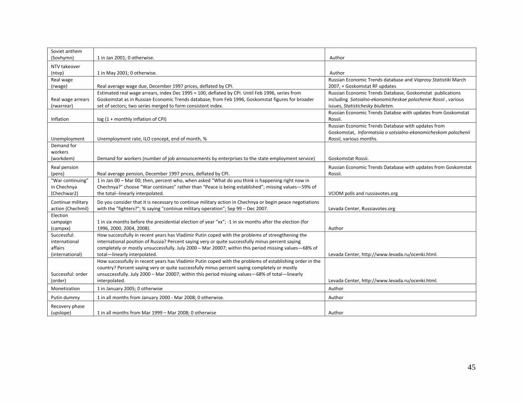
45

Soviet anthem (Sovhymn)  1 in Jan 2001; 0 otherwise.   Author 

NTV takeover (ntvp)  1 in May 2001; 0 otherwise.    Author 

Real wage (rwage)  Real average wage due, December 1997 prices, deflated by CPI. 

Russian Economic Trends database and Voprosy StatistikiMarch 2007, + Goskomstat RF updates 

Real wage arrears (rwarrear) 

Estimated real wage arrears, index Dec 1995 = 100, deflated by CPI. Until Feb 1996, series from Goskomstat as in Russian Economic Trends database; from Feb 1996, Goskomstat figures for broader set of sectors; two series merged to form consistent index. 

Russian Economic Trends Database, Goskomstat  publications including  Sotsialno‐ekonomicheskoe polozhenie Rossii , various issues, Statistichesky biulleten. 

Inflation  log (1 + monthly inflation of CPI) Russian Economic Trends Databse with updates from Goskomstat Rossii. 

Unemployment  Unemployment rate, ILO concept, end of month, % 

Russian Economic Trends Database with updates from Goskomstat,  Informatsiia o sotsialno‐ekonomicheskom polozhenii Rossii, various months. 

Demand for workers (workdem)  Demand for workers (number of job announcements by enterprises to the state employment service)  Goskomstat Rossii.  

Real pension (pens)  Real average pension, December 1997 prices, deflated by CPI. 

Russian Economic Trends Database with updates from Goskomstat Rossii. 

“War continuing” in Chechnya (Chechwar2) 

1 in Jan 00 – Mar 00; then, percent who, when asked “What do you think is happening right now in Chechnya?” choose “War continues” rather than “Peace is being established”; missing values—59% of the total‐‐linearly interpolated.  VCIOM polls and russiavotes.org 

Continue military action (Chechmil) 

Do you consider that it is necessary to continue military action in Chechnya or begin peace negotiations with the "fighters?"; % saying "continue military operation”; Sep 99 – Dec 2007.  Levada Center, Russiavotes.org 

Election campaign (campxx) 

1 in six months before the presidential election of year “xx”; ‐1 in six months after the election (for 1996, 2000, 2004, 2008).  Author 

Successful: international affairs (international) 

How successfully in recent years has Vladimir Putin coped with the problems of strengthening the international position of Russia? Percent saying very or quite successfully minus percent saying completely or mostly unsuccessfully. July 2000 – Mar 20007; within this period missing values—68% of total—linearly interpolated.   Levada Center, http://www.levada.ru/ocenki.html. 

Successful: order (order) 

How successfully in recent years has Vladimir Putin coped with the problems of establishing order in the country? Percent saying very or quite successfully minus percent saying completely or mostly unsuccessfully. July 2000 – Mar 20007; within this period missing values—68% of total—linearly interpolated.   Levada Center, http://www.levada.ru/ocenki.html. 

Monetization  1 in January 2005; 0 otherwise  Author 

Putin dummy  1 in all months from January 2000 ‐ Mar 2008; 0 otherwise.   Author 

Recovery phase (upslope)  1 in all months from Mar 1999 – Mar 2008; 0 otherwise  Author