presented at the comsol conference 2009 boston benchmarking comsol … · 2009-12-01 ·...
TRANSCRIPT

Benchmarking COMSOL Multiphysics 3.5a – CFD problems
Darrell W. Pepper
Xiuling Wang*
Nevada Center for Advanced Computational MethodsUniversity of Nevada Las Vegas
*Purdue University - Calumet
Boston MA, Oct. 8-10, 2009
Presented at the COMSOL Conference 2009 Boston

Xiuling Wang, PhD
Testing the mesh generator

Verification vs validation
Verification = solving the eqns right
Validation = solving the right eqns
Benchmarking = validating the verification

Outline
Introduction
Benchmark environment and criteria
Simulation results1. Flow over a 2-D circular cylinder2. Compressible flow in a shock tube3. Incompressible heated laminar flow and non-
heated turbulent flow over a 2-D backward facing step
4. 3D natural convection within an air-filled articulated cubical enclosure
Conclusions

Introduction
Objective Compare results obtained from COMSOL
Multiphysics 3.4 with those obtained from COMSOL Multiphysics 3.5a for four multiphysics problems
Test four CFD and CHT problems using COMSOL Multiphysics 3.5a
Obtain the CPU times and memory costs for solving those problems
New features for COMSOL 3.5a – segregated solver; 32 – 64 bit; memory saving 50%

Benchmark environment and criteria
Hardware: Platform 1: Pentium(R) D CPU 2.80GHz,
4.0GB this configuration was used to test the first four benchmark problems.
Platform 2: Intel ® Core ™ 2 Quad CPU Q9300 CPU 2.50GHz, 4.0GB RAM. This configuration was used for the four CFD-CHT benchmark problems.

Benchmark environment and criteria
Operating system: for the first hardware platform, the operating system was 32 bit and running Windows XP; for the second hardware platform, the operating system was 64 bit running Windows Vista.

Benchmark environment and criteria
Benchmark criteria Computational accuracy (comparison difference is
less than or equal to 5%) Contours of key variables Extreme values Experimental data
Mesh independent study Comparisons are made for results obtained for different
mesh densities for a selected test problem Increase in the number of elements leads to negligible
differences in the solutions.

Benchmark environment and criteria-cont.
Benchmark criteria Memory
Provided by software package whenever possible COMSOL “Mem Usage” shows the approximate memory
consumption, the average memory during the entire solution procedure
CPU time Execution times can be recorded from immediate access
to the CPU time by the program or from measuring wall-clock time
To obtain accurate CPU time, all unnecessary processes were stopped

Comparison between 3.4 and 3.5a
Benchmark
case
Software
Used
Number of elements
Memory cost (MB)
CPU time (s) Compared values
Case 1:
FSI
COMSOL Multiphysics 3.4
3,407 245 1,537 Totdis-max:25.43µm 6,602 267 3,342 Totdis-max:25.72µm9,728 308 5,301 Totdis-max:25.50µm14,265 349 8,475 Totdis-max:26.04µm
COMSOL Multiphysics 3.5
3,372 264 240 Totdis-max:21.97µm 6,221 290 522 Totdis-max:23.99µm9,918 295 719 Totdis-max:23.72µm20,545 320 2426 Totdis-max:25.14µm
Case 2:
Actuator
COMSOL Multiphysics 3.4
5,032 220 5 Xdis-max=3.065µm9,635 312 11 Xdis-max=3.069µm15,774 520 22 Xdis-max=3.066µm
COMSOL Multiphysics 3.5
5,032 170 3 Xdis-max=3.065µm10,779 360 8 Xdis-max=3.067µm16,893 480 22 Xdis-max=3.066µm
Case 3:
Circulator
COMSOL Multiphysics 3.4
9,067 173 127 reflection, isolation and insertion loss19,398 376 361
COMSOL Multiphysics 3.5
14,089 280 103
Case 4:
Generator
COMSOL Multiphysics 3.4
38,440 303 78 Bmax=1.225T
COMSOL Multiphysics 3.5
32,395 190 17 Bmax=1.257T

CFD-CHT problem 1 - Flow around a circular cylinder The flow around a circular cylinder has been examined
over many years and is a popular CFD demonstration problem. At very low Reynolds numbers, the flow is steady. As the Reynolds number is increased, asymmetries and time-
dependent oscillation develops in the wake region, resulting in the well-known Karman vortex street.
Problem configuration

CFD-CHT problem 1 - Flow around a circular cylinder –cont.
Re = 100, results from t = 0 s to t = 17 s. Mesh independent study
Number of
elements
Number of degrees of freedom
CPU time (s)
Memory (MB)
Mesh 1: 8,568
39,306 3,728 884
Mesh 2: 14,965
68,105 14,236 1,193
Mesh 1 Mesh 2

CFD-CHT problem 1 - Flow around a circular cylinder –cont.
Velocity fields from mesh 1 Velocity fields from mesh 2
Re = 100

CFD-CHT problem 1 - Flow around a circular cylinder –cont.
Drag coefficient from mesh 1 Drag coefficient from mesh 2
COMSOL 3.5a Mesh 1
COMSOL 3.5a Mesh 2
Numerical Results [5]
1.486 1.485 1.3353
Comparison of drag coefficient for Re = 100 with literature data [5]
[5] B. N. Rajani, A. Kandasamy and Sekhar Majumdar, “Numerical simulation of laminar flow past a circular cylinder”, Applied Mathematical Modelling, 33, pp. 1228-1247, 2009.

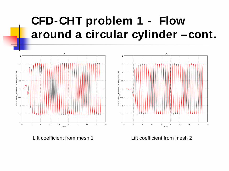
CFD-CHT problem 1 - Flow around a circular cylinder –cont.
Lift coefficient from mesh 1 Lift coefficient from mesh 2
Re = 100

CFD-CHT problem 1 - Flow around a circular cylinder –cont.
Re = 1,000, results from t = 0 s to t = 17 s. Mesh independent study
Mesh 1 Mesh 2
Number of
elements
Number of degrees of freedom
CPU time (s)
Memory (MB)
Mesh 1: 8,272
37,974 1,894 974
Mesh 2: 17,536
79,947 4,024 1,501

CFD-CHT problem 1 - Flow around a circular cylinder –cont.
Velocity fields from mesh 1 Velocity fields from mesh 2
Re = 1000

CFD-CHT problem 1 - Flow around a circular cylinder –cont.
Drag coefficient from mesh 1 Drag coefficient from mesh 2
COMSOL 3.5a Mesh 1
COMSOL 3.5a Mesh 2
Numerical Results [6]
1.69 1.65 1.47
Comparison of drag coefficient with literature data [6]
[6] G. Sod, “A survey of finite difference methods for systems of nonlinear hyperbolic conservation laws”, Journal of Computational Physics, 27, pp.1-31, 1978.
CFD-CHT problem 1 - Flow around a circular cylinder –cont.
Lift coefficient from mesh 1 Lift coefficient from mesh 2

Flow over a cylinder Re = 100

Re = 1000

Natural convection within a cylinder

CFD-CHT problem 2 -Compressible flow in a shock tube
Shock waves arise from sudden jumps in gas properties such as temperature or pressure. They are very thin regions (~10-8 m) in a supersonic flow across which there is a large variation in flow properties.
The configuration of problem is shown in the figure below, the diaphragm is located at x = 0.5.

CFD-CHT problem 2 -Compressible flow in a shock tube –cont.
The initial conditions for the driver section were and ;the initial condition for the driven section was
Results were obtained and compared with analytical solutions as well as simple numerical models based on MacCormack and Roe’s methods for t = 0.2.
Computational meshes
8.0; 7.2Pρ = =
; 0.0u =1.0; 0.72; 0.0P uρ = = =
Number of elements for coarse mesh
Number of degrees of
freedom for coarse mesh
Number of elements for final
fine mesh
Number of degrees of
freedom for final fine mesh
250 3,213 800 9,963250 3,213 4000 48,843

CFD-CHT problem 2 -Compressible flow in a shock tube –cont.
•Coarse Mesh
•Fine mesh 1 • Fine mesh 2
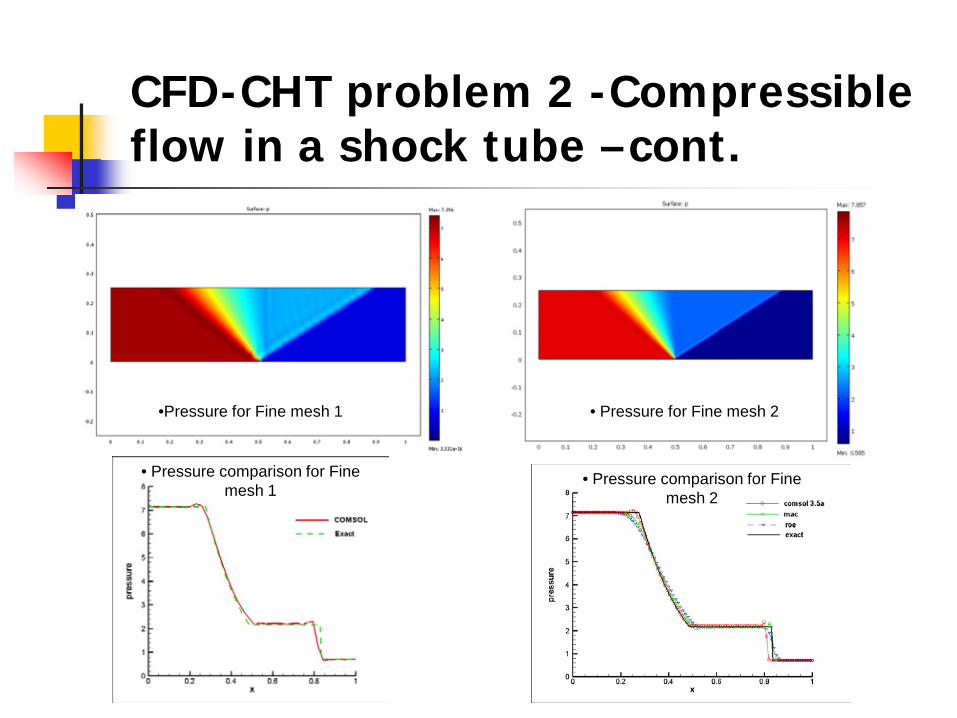
CFD-CHT problem 2 -Compressible flow in a shock tube –cont.
•Pressure for Fine mesh 1 • Pressure for Fine mesh 2
• Pressure comparison for Fine mesh 1
• Pressure comparison for Fine mesh 2

CFD-CHT problem 2 -Compressible flow in a shock tube –cont.
• Velocity for Fine mesh 1 • Velocity for Fine mesh 2
• Velocity comparison for Fine mesh 1 • Velocity comparison for Fine mesh 2

CFD-CHT problem 2 -Compressible flow in a shock tube –cont.
• Density for Fine mesh 1 • Density for Fine mesh 2
• Density Comparison for Fine mesh 1 • Density Comparison for Fine mesh 2

CFD-CHT problem 3 - Flow over a backward facing step
Incompressible flow over a backward facing step is a classic problem that has been analyzed for many years. While there are numerous fluid flow comparison studies, very few include the effects of heat transfer.
First test case is run as Re = 800 for thermal and fluid flow; second test case is run for Re = 47,648 for fluid flow only. The configuration of problem is shown as:
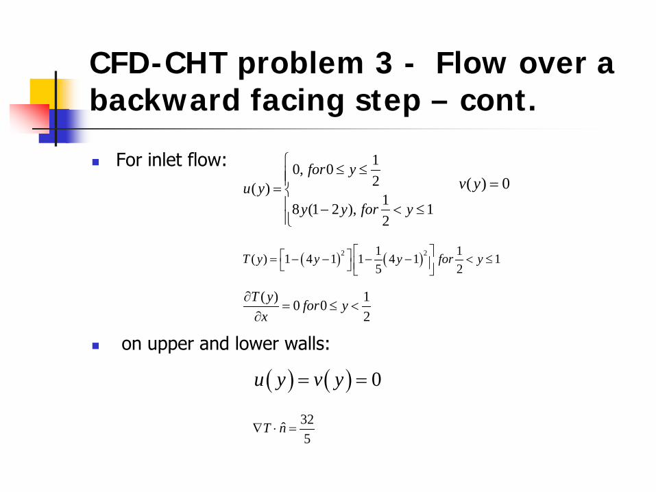
CFD-CHT problem 3 - Flow over a backward facing step – cont.
For inlet flow:
on upper and lower walls:
10, 02( )
18 (1 2 ), 12
for yu y
y y for y
≤ ≤= − < ≤
( ) 0v y =
( ) ( )2 21 1( ) 1 4 1 1 4 1 15 2
T y y y for y = − − − − < ≤
( ) 10 02
T y for yx
∂= ≤ <
∂
( ) ( ) 0u y v y= =
32ˆ5
T n∇ ⋅ =

CFD-CHT problem 3 - Flow over a backward facing step – cont.
Re = 800Number of elements
Number of degrees of freedom
CPU time (s)
Memory (MB)
Mesh 1: 10,850
108,864 2 298
Mesh 2: 22,000
288,384 3 350
•mesh 1 •mesh 2
Notice the fine mesh used along the boundary and in regions close to the step

CFD-CHT problem 3 - Flow over a backward facing step – cont.
Re = 800
•Velocity fields from mesh 1 •Velocity fields from mesh 2

CFD-CHT problem 3 - Flow over a backward facing step – cont.
•Streamlines from mesh 1 •Streamlines from mesh 2
COMSOL 3.5a Mesh 1
COMSOL 3.5a Mesh 2
Gartling [12]
Wang and Pepper [13]
6.80 6.70 6.1 6.0
Comparison of lower wall eddy sizes with literature data [12] [13]
[12] D. K. Gartling, “A Test Problem for Outflow Boundary Conditions- Flow over a Backward-Facing Step”, Int. J. Numer. Meth. Fluids, Vol. 11, pp. 953-967, 1990.[13] X. Wang and D. W. Pepper, “Application of an hp-adaptive FEM for Solving Thermal Flow Problems”, Journal of Thermophysics and Heat Transfer, Vol. 21, No. 1, pp.190-198, 2007.
Re = 800

CFD-CHT problem 3 - Flow over a backward facing step – cont.
Re = 47,648
•Initial mesh 1 •Initial mesh 2
Initial Number of elements
Initial Number of degrees of freedom
Final Number
of elements
Final Number of degrees of freedom
CPU time (s)
Memory (MB)
Mesh 1: 291 2,861 3,876 34,373 52 233Mesh 2: 585 5,504 8,734 76,701 119 350
•Adapted mesh 1 •Adapted mesh 2

CFD-CHT problem 3 - Flow over a backward facing step – cont.
Re = 47,648
•Velocity fields from mesh 1 •Velocity fields from mesh 2

CFD-CHT problem 3 - Flow over a backward facing step – cont.
•Streamlines from mesh 1 •Streamlines from mesh 2
Comparison of lower wall eddy sizes with literature data [14] [15]
[14] 1st NAFEMS Workbook of CFD Examples. Laminar and Turbulent Two-Dimensional Internal Flows, NAFEMS, 2000.[15]Patrick J. Roache, Verification and Validation in Computational Science and Engineering, Hermosa Pub., Albuquerque, NM, 1998.
Re = 47,648
COMSOL 3.5a Mesh 1
COMSOL 3.5a Mesh 2
Experimental data
Other simulation
results6.0 6.19 7.1 6.1
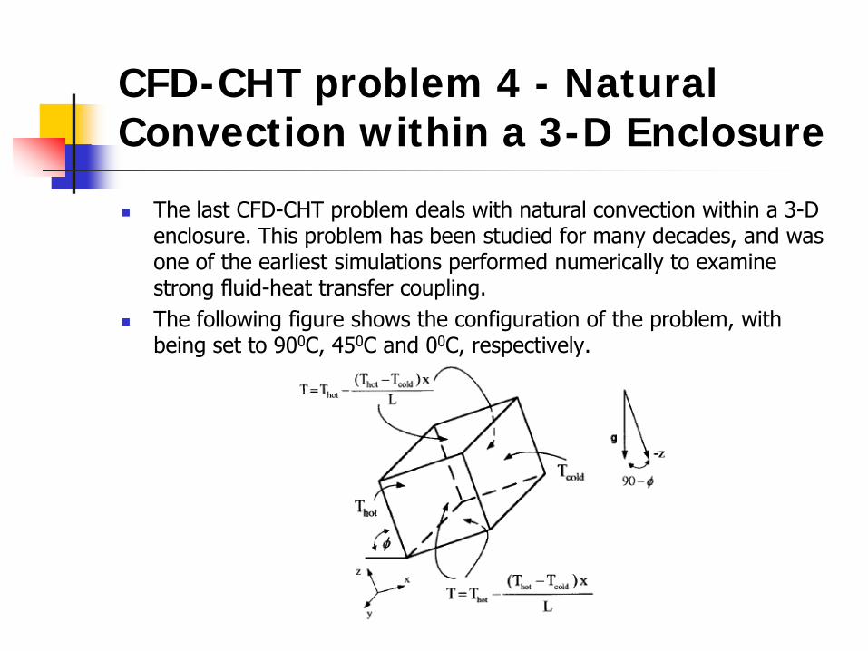
CFD-CHT problem 4 - Natural Convection within a 3-D Enclosure
The last CFD-CHT problem deals with natural convection within a 3-D enclosure. This problem has been studied for many decades, and was one of the earliest simulations performed numerically to examine strong fluid-heat transfer coupling.
The following figure shows the configuration of the problem, with being set to 900C, 450C and 00C, respectively.

CFD-CHT problem 4 - Natural Convection within a 3-D Enclosure –cont.
Case 1: φ = 90o
Number of elements for coarse mesh
Number of degrees of freedom for coarse mesh
Number of elements for final
fine mesh
Number of degrees of freedom for final fine mesh
1,000 38,375 8,000 284,945
• Final Computational mesh

CFD-CHT problem 4 - Natural Convection within a 3-D enclosure –cont.
Case 1: φ = 90o Ra = 105 at y = L/2
• Temperature contours • Velocity vectors
Results from COMSOL 3.5a
[16] [17] [18] [19]
3.12 3.11 3.06-3.12 3.10 3.19-3.20
Comparison of Nu with literature data [16-19]

CFD-CHT problem 4 - Natural Convection within a 3-D enclosure –cont.
Case 2: φ = 45o Ra = 105 at y = L/2
• Temperature contours • Velocity vectors
Results from COMSOL 3.5a
[16] [17] [18] [19]
3.54 - 3.40-3.47 3.50 3.57-3.60
Comparison of Nu with literature data [16-19]

CFD-CHT problem 4 - Natural Convection within a 3-D enclosure –cont.
Case 3: φ = 0o Ra = 105 at y = L/2
• Temperature contours • Velocity vectors
Results from COMSOL 3.5a
[16] [17] [18] [19]
2.25 3.24 3.34-3.47 2.49-3.92 3.49-4.01
Comparison of Nu with literature data [16-19]

CFD-CHT problem 4 - Natural Convection within a 3-D enclosure –cont.
[16] R. Bennacer, A. A. Mohamad, and I. Sezai, Transient Natural Convection in Air-Filled Cubical Cavity: Validation Exercise, ICHMT 2nd Int. Symp. on Adv. in Comput. Heat Transfer, Palm Cove, Queensland, Australia, May 20– 25, 2001.
[17] R. Mossad, Prediction of Natural Convection in an Air-Filled Cubical Cavity Using Fluent Software, ICHMT 2nd Int. Symp. on Adv. in Comput. Heat Transfer, Palm Cove, Queensland, Australia, May 20– 25, 2001.
[18] E. Krepper, CHT’01: Validation Exercise: Natural Convection in an Air-Filled Cubical Cavity, ICHMT 2nd Int. Symp. on Adv. in Comput. Heat Transfer, Palm Cove, Queensland, Australia, May 20– 25, 2001.
[19] C. Xia, J. Y. Murthy, and S. R. Mathur, Finite Volume Computations of Buoyancy- Driven Flow in a Cubical Cavity: A Benchmarking Exercise, ICHMT 2nd Int. Symp. On Adv. in Comput. Heat Transfer, Palm Cove, Queensland, Australia, May 20– 25, 2001.

Conclusions Comparison between running COMSOL 3.5a on 32 bit machine
vs. on 64 bit machine
Number of elements
CPU time (s) (32 bit
machine)
CPU time (s) (64 bit
machine)
Memory (MB) (32 bit
machine)
Memory (MB) (64 bit
machine)Mesh 1: 10,850 3.79 2 211 298Mesh 2: 22,000 6.958 3 303 350
Comparison of flow over backward facing step Re = 800 from COMSOL 3.5a
Initial Number of elements
Initial Number of degrees of freedom
Final Number of elements
Final Number of degrees of freedom
CPU time (s)(64bit)
CPU time (s)
(32bit)
Memory (MB)
(64bit)
Memory (MB)
(32bit)
Mesh 1: 291 2,861 3,876 34,373 52 133.817 233 250
Mesh 2: 585 5,504 8,734 76,701 119 313.45 350 322
Comparison of flow over backward facing step Re = 47,648 from COMSOL 3.5a

Conclusions –cont.Benchmark
case
Number of elements
Number of degrees of freedom
CPU time (s) Memory cost (MB)
Compared valuesCOMSOL
resultsLiterature data
Case 1-a: Flow over circular cylinder Re = 100
8,568 39,306 3,728 884 Cd = 1.486 Cd = 1.3353 see [5] 14,965 68,105 14,236 1,193 Cd = 1.485
Case 1-b: Flow over circular cylinder Re = 1000
8,272 37,974 1,894 974 Cd = 1.69 Cd = 1.47 see [6]17,536 79,947 4,024 1,501 Cd = 1.65
Case 2: Compressible flow in a shock tube
800 9,963 Multi-grid scheme has been applied
Pressure, velocity and density are compared with analytical
solution (Fig. 33, 34, 35)4000 48,843
Case 3-a: Flow over a backward facing step Re = 800
10,850 108,864 2 298 Lloweddy = 6.8 Lloweddy = 6.1 [12]; Lloweddy = 6.0 [13]
22,000 288,384 3 350 Lloweddy = 6.7
Case 3-b: Flow over a backward facing step Re = 47,648
3,876 34,373 52 233 Lloweddy = 6.0 Lloweddy = 7.1 [14]; Lloweddy = 6.1 [15]
8,734 76,701 119 350 Lloweddy = 6.19
Case 4-a: Natural convection within a 3D enclosure φ = 90o
8,000 284,945 Multi-grid scheme has been applied
Nu = 3.12 3.10 [18]
Case 4-b: Natural convection within a 3D enclosure φ = 45o
8,000 284,945 Multi-grid scheme has been applied
Nu = 3.54 3.50 [18]
Case 4-c: Natural convection within a 3D enclosure φ = 0o
8,000 284,945 Multi-grid scheme has been applied
Nu = 2.25 2.49-3.92 [18]

Comparison between XXXXXX, COMSOL and Literature Data
Benchmark
case
Number of cells CPU time (s) Compared valuesXXXXXX COMSOL Literature
Case 1-a: Flow over circular cylinder Re = 100
16,689
14,955
2,245
3,728
14,236
Cd = 1.479 Cd = 1.485 Cd = 1.3353 see [5]
Case 1-b: Flow over circular cylinder Re = 1000
16,689
17,536
2,425
1,894
4,024
Cd = 1.55 Cd = 1.65 Cd = 1.47 see [6]
Case 2: Compressible flow in a shock tube
40 in x-dir Density, velocity and pressure are compared with analytical solutions (Fig. 9, 10, 11)200 in x-dir
Case 3-a: Flow over a backward facing step Re = 800
12,000 Final report Lloweddy = 6.82 Lloweddy = 6.70 Lloweddy = 6.1 [12]; Lloweddy = 6.0 [13]
Case 3-b: Flow over a backward facing step Re = 47,648
9,600 Final report Lloweddy = 7.0 Lloweddy = 6.19 Lloweddy = 7.1 [14]; Lloweddy = 6.1 [15]
Case 4-a: Natural convection within a 3D enclosure φ = 90o
32,000 Final report Nu = 3.10 Nu = 3.12 3.10 [18]
Case 4-b: Natural convection within a 3D enclosure φ = 45o
32,000 Final report Nu = 3.43 Nu = 3.54 3.50 [18]
Case 4-c: Natural convection within a 3D enclosure φ = 0o
32,000 Final report Nu = 3.43 Nu = 2.25 2.49-3.92 [18]
The Future
COMSOL 4 Compare results obtained from COMSOL
Multiphysics 4 with those obtained from COMSOL Multiphysics 3.5a and other data
Obtain the CPU times and memory costs Try parallel version on Cray CX1
What’s coming: multiscale, multiphysics, stochastic modeling
Advances in h-p adaptation; meshless methods

UAV - 2008

SolidWorks - COMSOL

The Flight of COMSOL- I


Contacts
Darrell W. PepperNCACMUniversity of Nevada Las [email protected]
Xiuling WangDepartment of Mechanical EngineeringPurdue University – [email protected]