Full Terms & Conditions of access and use can be found athttp://www.tandfonline.com/action/journalInformation?journalCode=lsta20

Download by: [University of California Santa Barbara] Date: 31 March 2016, At: 12:32

Communications in Statistics - Theory and Methods

ISSN: 0361-0926 (Print) 1532-415X (Online) Journal homepage: http://www.tandfonline.com/loi/lsta20

Analysis of Gamma and Weibull Lifetime Dataunder a General Censoring Scheme and in thepresence of Covariates

Nathan Bennett, Srikanth K. Iyer & S. Rao Jammalamadaka

To cite this article: Nathan Bennett, Srikanth K. Iyer & S. Rao Jammalamadaka (2016): Analysisof Gamma and Weibull Lifetime Data under a General Censoring Scheme and in the presenceof Covariates, Communications in Statistics - Theory and Methods

To link to this article: http://dx.doi.org/10.1080/03610926.2015.1041981

Accepted author version posted online: 31Mar 2016.

Submit your article to this journal

View related articles

View Crossmark data

ACCEPTED MANUSCRIPT

Analysis of Gamma and Weibull Lifetime Data under a General Censoring Scheme and in

the presence of Covariates

by

Nathan Bennett

Department of Statistics and Applied Probability, University of California, Santa Barbara, CA

93106,

Srikanth K. Iyer1

Department of Mathematics, Indian Institute of Science, Bangalore, India,

and

S. Rao Jammalamadaka

Department of Statistics and Applied Probability, University of California, Santa Barbara, CA

93106.

Abstract1Corresponding Author. email: srikiyer@gmail.com. Research supported in part by UGC CAS.

1ACCEPTED MANUSCRIPT

Dow

nloa

ded

by [

Uni

vers

ity o

f C

alif

orni

a Sa

nta

Bar

bara

] at

12:

32 3

1 M

arch

201

6

ACCEPTED MANUSCRIPT

We consider the problem of estimating the lifetime distributions of sur-

vival times subject to a general censoring scheme called ”middle censor-

ing”. The lifetimes are assumed to follow a parametric family of distri-

butions, such as the Gamma or Weibull distributions, and is applied to

cases when the lifetimes come with covariates affecting them. For any

individual in the sample, there is an independent, random, censoring in-

terval. We will observe the actual lifetime if the lifetime falls outside of

this censoring interval, otherwise we only observe the interval of cen-

soring. This censoring mechanism, which includes both right- and left-

censoring, has been called ”middle censoring” (see Jammalamadaka and

Mangalam (2003)). Maximum likelihood estimation of the parameters

as well as their large sample properties are studied under this censoring

scheme, including the case when covariates are available. We conclude

with an application to a dataset from Environmental Economics dealing

with Contingent Valuation of natural resources.

Keywords: Middle censoring, Maximum likelihood estimators, Accelerated failure time model,

EM algorithm, Gamma distribution, Weibull distribution.

2ACCEPTED MANUSCRIPT

Dow

nloa

ded

by [

Uni

vers

ity o

f C

alif

orni

a Sa

nta

Bar

bara

] at

12:

32 3

1 M

arch

201

6

ACCEPTED MANUSCRIPT

1 Introduction

Our aim in this paper is to estimate the lifetime distribution or its complement, the survival func-

tion, for data that is subject to middle censoring. Middle censoring occurs when a data point

becomes unobservable if it falls inside a random interval. This is a generalization of left and right

censored data and is quite distinct from the case of doubly censored data. We consider two fami-

lies of distributions that are common to many applications, namely the Gamma distribution or the

Weibull distribution.

Middle censoring was first introduced by Jammalamadaka and Mangalam (2003) for non-

parametric estimation of the lifetime distributions, and was studied further in Jammalamadaka

and Iyer (2004). Middle censored data was analyzed in Iyer, Jammalamadaka, and Kundu (2008)

when the lifetimes are exponentially distributed, whereas Jammalamadaka and Mangalam (2009)

study such censoring in the context of circular data. Gamma and Weibull distributions are natural

and the most widely used choices for modelling lifetimes in many applications. Not only does

the consideration of these more general models extend the earlier results for the exponential dis-

tribution in Iyer, Jammalamadaka, and Kundu (2008), but the current work also discusses how the

presence of covariates can be handled nicely in the form of Accelerated Failure Time (AFT) mod-

elling (see Section 3). We derive the maximum likelihood estimators for the parameters and show

how the computation of the MLEs can be done via the EM algorithm. We then establish their large

sample properties.

Let us denote the ”actual” lifetimes ofn individuals by t1, ∙ ∙ ∙ , tn, and not all of them are

observable. For each individual there is a random period of time[`i , ri] for which the lifetime

of the ith individual is unobservable. Thus, the actual lifetime is observed ifti < [`i , ri] and if

ti ∈ [`i , ri] then only the interval is observed. Hence the observed data is given by:

(xi , δi) =

(ti ,1) i f ti < [`i , ri]

([`i , ri] ,0) otherwise(1.1)

Based on observed data of this type, the goal is to estimate the lifetime distribution function. The

3ACCEPTED MANUSCRIPT

Dow

nloa

ded

by [

Uni

vers

ity o

f C

alif

orni

a Sa

nta

Bar

bara

] at

12:

32 3

1 M

arch

201

6

ACCEPTED MANUSCRIPT

lifetimes are assumed to be independent and identically distributed(i.i.d.) from an unknown dis-

tribution functionF (∙). Additionally, the censoring intervals,[L1, R1] , ∙ ∙ ∙ , [Ln, Rn], are assumed

to be i.i.d. from an unknown bivariate distribution functionG (∙, ∙). Finally, the lifetimes and the

censoring intervals are taken to be independent of each other, as is common in survival analysis.

In Section 2 we consider the Maximum Likelihood estimation of the parameters for these 2

models under middle censoring, discuss the EM algorithm needed for their computation, and es-

tablish asymptotic properties like consistency and asymptotic normality of these estimators. In

Section 3, we consider estimation under middle-censoring in the presence of covariates employing

Accelerated Failure Time modelling. Extensive simulations illustrate the robustness of these MLEs

even under heavy censoring.

2 Maximum Likelihood Estimation

The lifetimes are assumed to follow either a Gamma or a Weibull distribution whose respective

probability density functions are given by

f1(t| a, b) =ba

Γ(a)ta−1e−bt f or t > 0, (2.2)

f2(t| a, b) = aba ta−1 exp[−ba ta] f or t > 0, (2.3)

and (a,b) ∈ Θ = [0,∞)2.The unknown censoring distributionG is then assumed to be supported

on [0,∞)2. The data can be re-arranged so that the firstn1 observations are uncensored and the last

n2 observations are censored. Then the respective log-likelihood functions for these two models

are given by

l1n(a, b) = an1 ln b− n1 ln (Γ(a)) + (a− 1)n1∑

i=1

ln (ti) − bn1∑

i=1

ti

+

n1+n2∑

i=n1+1

ln [F1 (ri | a, b) − F1 (li | a, b)] . (2.4)

4ACCEPTED MANUSCRIPT

Dow

nloa

ded

by [

Uni

vers

ity o

f C

alif

orni

a Sa

nta

Bar

bara

] at

12:

32 3

1 M

arch

201

6

ACCEPTED MANUSCRIPT

whereF1(t| a, b) is the CDF of a Gamma(a, b) distribution.

l2n(a, b) = n1 ln a+ n1a ln b+ (a− 1)n1∑

i=1

ln (ti) − ban1∑

i=1

tai

+

n1+n2∑

i=n1+1

ln(exp

[−balai

]− exp

[−bara

i

])(2.5)

Let θ = (a,b) denote the unknown parameter vector. The MLEθ̂ of θ is the value of the pa-

rameter which maximizes the function in (2.4), (2.5) respectively for the case of the Gamma and

Weibull distributions. We first discuss the large sample properties of these estimators followed by

computational aspects.

2.1 Large-sample properties of the MLEs

Our approach in this section is similar to that of Jammalamadaka and Mangalam (2009). Recall

that the censoring mechanism is independent of the lifetime distributions. Conditional on the

censoring interval (̀, r), define the censoring probability by

pi(θ, `, r) = P(T ∈ (`, r)) =∫ r

`

fi(t|θ)dt, i = 1,2. (2.6)

Let θ0 denote the true value of the parameter. For convenience, we will work with the parameterb

replaced byc−1. Define the functions

g1(θ, `, r) = −a ln(c) − ln (Γ(a)) +∫

t<(`,r)ln

(ta−1e−t/c

)f1(t|θ0)dt

+ p1(θ0, `, r) ln

(∫ r

`

ta−1e−t/cdt

)

, (2.7)

g2(θ, `, r) = ln(a) − a ln(c) +∫

t<(`,r)ln

(ta−1e−ta/ca)

f2(t|θ0)dt

+ p2(θ0, `, r) ln

(∫ r

`

ta−1e−ta/cadt

)

(2.8)

Define the function

hi(θ) =∫

gi(θ, `, r)dG(`, r), i = 1,2. (2.9)

5ACCEPTED MANUSCRIPT

Dow

nloa

ded

by [

Uni

vers

ity o

f C

alif

orni

a Sa

nta

Bar

bara

] at

12:

32 3

1 M

arch

201

6

ACCEPTED MANUSCRIPT

Lemma 2.1 For i = 1,2, we have1nlin(θ)→ hi(θ), Pθ0−a.s.

Proof. Fork = 1,2, . . ., define the sequences of random variables

X1k = −a ln(c) − ln (Γ(a)) + δk ln

(ta−1k e−tk/c

)+ (1− δk) ln

(∫ rk

`k

ta−1e−t/cdt

)

, (2.10)

X2k = ln(a) − a ln(c) + δk ln

(ta−1k e−tak/c

a)+ (1− δk) ln

(∫ rk

`k

ta−1e−ta/cadt

)

. (2.11)

The above two sequences are i.i.d. with meanhi(θ) i = 1,2 respectively underPθ0. The result thus

follows from the law of large numbers.

The following Lemma is a restatement of Lemma 3.3 in Jammalamadaka and Mangalam

(2009).

Lemma 2.2 If ` and r are two distinct arbitrary points in(0,∞), then gi(θ, `, r) ≤ gi(θ0, `, r)

i = 1,2, for all θ ∈ Θ with equality holding only whenθ = θ0.

Theorem 2.3 If the identifiability condition

p(θ0) = Pθ0(T ∈ (L,R)) < 1,

holds, then̂θ → θ0, Pθ0−a.s.

Proof. From Lemma 2.2, it follows thathi(θ) ≤ hi(θ0) for all θ ∈ Θ with equality holding only

whenθ = θ0.

Fix ε > 0 sufficiently small such thatε < c0 and restrict the range ofc to (ε,∞). By integrating

over the full range of the second integrals in (2.7), 2.8), we get

g1(θ, `, r) ≤ (−a ln(c) − ln (Γ(a)))(1− p1(θ0, `, r)) + u(θ, `, r),

g2(θ, `, r) ≤ (ln(a) − a ln(c))(1− p2(θ0, `, r)) + v(θ, `, r),

whereu, v are the first integrals on the right in (2.7), (2.8) respectively. Under the identifiability

condition,pi(θ0, `, r) < 1 on a set of positiveG measure. Hence,gi(θ, `, r) and hencehi(θ)→ ∞ as

6ACCEPTED MANUSCRIPT

Dow

nloa

ded

by [

Uni

vers

ity o

f C

alif

orni

a Sa

nta

Bar

bara

] at

12:

32 3

1 M

arch

201

6

ACCEPTED MANUSCRIPT

|θ| → ∞ in [0,∞) × [ε,∞), for i = 1,2. LetΩi0 be the set ofPθ0 measure 1 where1nlin(θ) → hi(θ),

i = 1,2. The argument below holds for bothi = 1,2 and hence we suppress the indexi. Fix any

ω ∈ Ω0. If θ̂n 9 θ0, then there is a subsequencenk through whichθ̂n → θ1 = (a1,b1), where

(a1,b1) ∈ [0,∞] × [ε,∞].

If |θ1| < ∞, then from Lemma 2.1,1nklnk(θ̂nk) → h(θ1). However, 1

nklnk(θ̂nk) ≥

1nk

lnk(θ0) → h(θ0)

leading to the conclusion thath(θ1) ≥ h(θ0), thus contradicting Lemma 2.2.

If |θ1| = ∞, then 1nk

lnk(θ̂nk) = limθ→θ1 h(θ) = −∞. Again, 1nk

lnk(θ̂nk) ≥1nk

lnk(θ0)→ h(θ0) leading to

a contradiction.

Theorem 2.4 LetΣ1 be the dispersion of(∂Xi

1∂a ,

∂Xi1∂b

), i = 1,2, where Xi

1 is defined in (2.10), (2.11).

Under the identifiability condition given in Theorem 2.3, we have√

n(θ̂n − θ0) ⇒ N2(0,Σ(θ0)),

whereΣ(θ) = [h′′(θ)]−1Σ1(θ)[h′′(θ)]−1.

Proof. The proof is fairly straightforward (see for example the proof of Theorem 3.2 in

Jammalamadaka and Mangalam (2009)) and so we omit it.

2.2 Computation of the MLEs

To compute the ML estimators, we need to maximize equations (2.4) in case of the Gamma distri-

bution and (2.5) if the underlying distribution is Weibull. We first describe the EM algorithm and

address the issue of convergence of the algorithm for a much wider class of distributions than the

ones considered in this paper. Computation of the MLE when the lifetimes are distributed accord-

ing to the Weibull distribution using the EM algorithm has been considered in Kundu and Pradhan

(2014).

Suppose thatx1, ∙ ∙ ∙ , xn1,(ln1+1, rn1+1

), ∙ ∙ ∙ ,

(ln1+n2, rn1+n2

)is the observed middle-censored data

from a continuous exponential family distribution withk parameters, namely they have probability

density function

f (x|φ) = h (x) c (φ) exp

k∑

j=1

wj (φ) vj (x)

, (2.12)

7ACCEPTED MANUSCRIPT

Dow

nloa

ded

by [

Uni

vers

ity o

f C

alif

orni

a Sa

nta

Bar

bara

] at

12:

32 3

1 M

arch

201

6

ACCEPTED MANUSCRIPT

whereh (x) , vj (x) , c (φ) , and wj (φ) are continuous functions. Note thatφ = (φ1, ∙ ∙ ∙ , φk) is ak

dimensional vector of parameters. This results in the following complete log-likelihood:

l (φ) = n log[c (φ)

]+

n1∑

i=1

log[h (ti)] +

k∑

j=1

wj (φ) vj (ti)

+

n1+n2∑

i=n1+1

log[h (ti)] +

k∑

j=1

wj (φ) vj (ti)

(2.13)

We wish to solve for the MLE ofφ, which will be done by implementing the EM algorithm. More

specifically, we will find the initial estimates forφ = (φ1, ∙ ∙ ∙ , φk) from the uncensored data, and

the estimates ofφ will be updated using the following procedure:

• Step 1: Suppose thatφ( j) = (φ1, ∙ ∙ ∙ , φk)( j) is the jth estimate

• Step 2: ComputeT∗i by calculatingE[Ti |ai < Ti < bi , φ = φ( j)

]

• Step 3: Solve Equation (2.13) with theT∗i ’s imputed for the censored observations for its

maximum and setφ( j+1) as the values that maximizes that equation.

• Step 4: Repeat until convergence criteria is met

We are now ready to prove that this algorithm does indeed converge.

Theorem 2.5 Let x1, ∙ ∙ ∙ , xn1,(ln1+1, rn1+1

), ∙ ∙ ∙ ,

(ln1+n2, rn1+n2

), be the observed middle-censored

data from a continuous exponential family distribution

f (x|φ) = h (x) c (φ) exp

k∑

j=1

wj (φ) t j (x)

such that h(x) , t j (x) , c (φ) , and wj (φ) are all continuous functions. Then the EM algorithm will

converge for this data.

Proof. The result follows by an application of the second theorem in Wu (1983) on the EM

algorithm. Note that the complete log-likelihood is proportional to

l (φ) ∝ n log[c (φ)

]+

n1∑

i=1

k∑

j=1

wj (φ) t j (xi) +n1+n2∑

i=n1+1

k∑

j=1

wj (φ) t j (xi)

8ACCEPTED MANUSCRIPT

Dow

nloa

ded

by [

Uni

vers

ity o

f C

alif

orni

a Sa

nta

Bar

bara

] at

12:

32 3

1 M

arch

201

6

ACCEPTED MANUSCRIPT

Also, observe that

E[t j (xi) |φ

∗, ai < xi < bi

]=

∫ bi

ai

t j (xi) h (xi) c (φ∗) exp

k∑

j=1

wj (φ∗) t j (xi)

dxi

is a continuous function. Thus

E[l (φ|complete data) |φ∗, censored data

]∝ n log

[c (φ)

]+

n1∑

i=1

k∑

j=1

wj (φ) t j (xi)

+

n1+n2∑

i=n1+1

k∑

j=1

wj (φ) E[t j (xi) |φ

∗, ai < xi < bi

]

is a continuous function in bothφ andφ∗. Thus by Theorem 2 of Wu (1983), it follows that the EM

algorithm will converge. We now move on to specific examples.

We first consider the case of the Gamma distribution. In this case the log-likelihood can be

written as

l(α, β) = an1 ln b− n1 ln (Γ(a)) + (a− 1)n1∑

i=1

ln (ti) − bn1∑

i=1

ti

+

n1+n2∑

i=n1+1

ln [F (ri | a, b) − F (li | a, b)] (2.14)

where andF(t| a, b) is the CDF of a Gamma(a, b) distribution. We now need the conditional expec-

tations for the incomplete data in order to use the EM algorithm. The two necessary expectations

are

E[T |L < T < R] =

∫ R

Lt ba

Γ(a) ta−1e−btdt

F1(R| a, b) − F1(L| a, b)(2.15)

E[ln T |L < T < R] =

∫ R

Lln t ba

Γ(a) ta−1e−btdt

F2(R| a, b) − F2(L| a, b)(2.16)

The above equation does not have a closed form solution and so we solve numerically to obtain the

solution. This can be used in the E-Step in the EM algorithm, and then the pseudo log-likelihood

will be

l∗(θ) = anln b− n ln (Γ(a)) + (a− 1)

n1∑

i=1

ln (ti) +n1+n2∑

i=n1+1

ln(t∗i)

9ACCEPTED MANUSCRIPT

Dow

nloa

ded

by [

Uni

vers

ity o

f C

alif

orni

a Sa

nta

Bar

bara

] at

12:

32 3

1 M

arch

201

6

ACCEPTED MANUSCRIPT

−b

n1∑

i=1

ti +n1+n2∑

i=n1+1

t∗i

(2.17)

where thet∗i ’s are found using Equations 2.15 & 2.16.

Thus the EM Algorithm can be set up as follows. Choose (a, b)(0) to be the MLE of the

uncensored data. Update the estimates with the following steps:

• Step 1: Suppose that (a, b)( j) is the jth estimate

• Step 2: ComputeT∗i using equation (2.15) & 2.16 with (a, b) = (a, b)( j)

• Step 3: Solve equation (2.17) for its maximum and set (a, b)( j+1) as that maximum

• Step 4: Repeat until convergence criteria is met

Since there is no explicit form for the MLE’s of a Gamma distribution, the maximum must either

be solved iteratively or with a built-in numerical solver.

The same procedure works for the case of the Weibull distribution. We re-labelba asb while

carrying out the simulations. In this case the log-likelihood for the Weibull lifetimes is given by

l(a, b) = n1 ln a+ n1 ln b+ (a− 1)n1∑

i=1

ln (ti) − bn1∑

i=1

tai

+

n1+n2∑

i=n1+1

ln(exp

[−blai

]− exp

[−bra

i

])(2.18)

The desired conditional expectations are given by

E[Ta|L < T < R] =

∫ R

Lta ab ta−1 exp[−b ta] dt

exp[−blai

]− exp

[−bra

i

] (2.19)

E[ln T |L < T < R] =

∫ R

Lln t ab ta−1 exp[−b ta] dt

exp[−blai

]− exp

[−bra

i

] (2.20)

This will lead to the following pseudo log-likelihood

l∗(a, b) ∝ n ln a+ n ln b+ (a− 1)

n1∑

i=1

ln (ti) +n1+n2∑

i=n1+1

ln(t∗i)

10ACCEPTED MANUSCRIPT

Dow

nloa

ded

by [

Uni

vers

ity o

f C

alif

orni

a Sa

nta

Bar

bara

] at

12:

32 3

1 M

arch

201

6

ACCEPTED MANUSCRIPT

−b

n1∑

i=1

tai +n1+n2∑

i=n1+1

(t∗i)a

(2.21)

The rest of the procedure is identical to the previous case.

3 Accelerated Failure Time Models

In this section we will consider the problem of ML estimation of the parameters of ap−parameter

Accelerated Failure Time (AFT) model where the baseline distribution is exponential, gamma or

Weibull distributed. The AFT models are known to be more robust to the estimation of covariate

effects (e.g. see Keiding and Andersen (1997)), and are more easy to interpret than hazard rates.

For instance in a clinical trial where mortality is the endpoint, one could translate the result as a

certain percentage increase in future life expectancy on the new treatment compared to the baseline.

As before suppose the middle censored data is in the form

t1, ∙ ∙ ∙ , tn1,(ln1+1, rn1+1

), ∙ ∙ ∙ ,

(ln1+n2, rn1+n2

)

Associated with each observation is an observed vectorZi representing the covariates. The ML

estimation is done as earlier using the EM algorithm, which requires the conditional expectation

of the unobserved data given that it falls in a particular interval. As before, the convergence of

the EM algorithm is a consequence of the continuity of the log-likelihood function. The respec-

tive probability density function of the observations for the three models, namely the exponential,

Gamma and Weibull are given below:

f (t|Z,a) = exp[θTZi

]exp

{−a exp

[θTZ i

]t}, t > 0, (3.22)

f (t|Z,a,b) =1

Γ (a)(b exp

[−θTZ

])a ta−1 exp

−t

b exp[−θTZ

]

, t > 0, (3.23)

f (t|Z,a,b) = a(b exp

[aθTZ

])ta−1 exp

[−

(b exp

[aθTZ

])ta], t > 0. (3.24)

11ACCEPTED MANUSCRIPT

Dow

nloa

ded

by [

Uni

vers

ity o

f C

alif

orni

a Sa

nta

Bar

bara

] at

12:

32 3

1 M

arch

201

6

ACCEPTED MANUSCRIPT

4 Simulation Study

To illustrate and validate the procedure, we simulate data under the assumption that the left end

point and the length of the censoring intervals are independent and exponentially distributed with

parametersα andβ respectively. For each sample sizen, N = 1000 samples were simulated. Each

sample was then censored, and the EM algorithm was applied to the censored data. Thea andb

estimates reported are the average value of theN = 1000 estimates obtained.

See Table 1 for the results of these simulations when the lifetimes are from a Gamma distri-

bution. The rowCensoredin the table provides the smallest proportion of censoring and largest

proportion of censoring in theN = 1000 simulated samples. The simulation results for the Weibull

case are summarized in Table 2. The estimates for the Weibull model also appear to converge very

well. The procedure performs reasonably well even with a large proportion of censored observa-

tions.

Also examined was the goodness of fit of the estimated model. To study this, a sample of

sizen=100 was created from a Gamma distribution. Using the aforementioned process, these data

were middle-censored, resulting in twenty-five percent of the data being censored. The MLEs

were calculated using the proposed EM algorithm. The empirical CDF of the uncensored data

and fitted CDF are given in Figure 1. The two curves appear to be very similar. Furthermore, a

Kolmogorov Smirnov test was performed using the fitted Gamma distribution and uncensored data

which yielded a p-value of 0.433 indicating no lack of fit.

A simulation study was performed to illustrate the usefulness of the approach outlined above

for the AFT models. Simulations were carried out in R usingN=1000 replications with a common

sample size ofn=100. The censoring mechanism is the same as used previously. Specifically, the

left endpoint of the censored interval is Exponentially distributed with mean 1; the length of the

censored interval is also Exponentially distributed with mean 1. Three covariate values were used.

The first two covariates,Z1 & Z2, were generated from a Binomial distribution with one trial and

probability of success equal to 0.5. The third covariate,Z3, was generated from a Standard Normal

12ACCEPTED MANUSCRIPT

Dow

nloa

ded

by [

Uni

vers

ity o

f C

alif

orni

a Sa

nta

Bar

bara

] at

12:

32 3

1 M

arch

201

6

ACCEPTED MANUSCRIPT

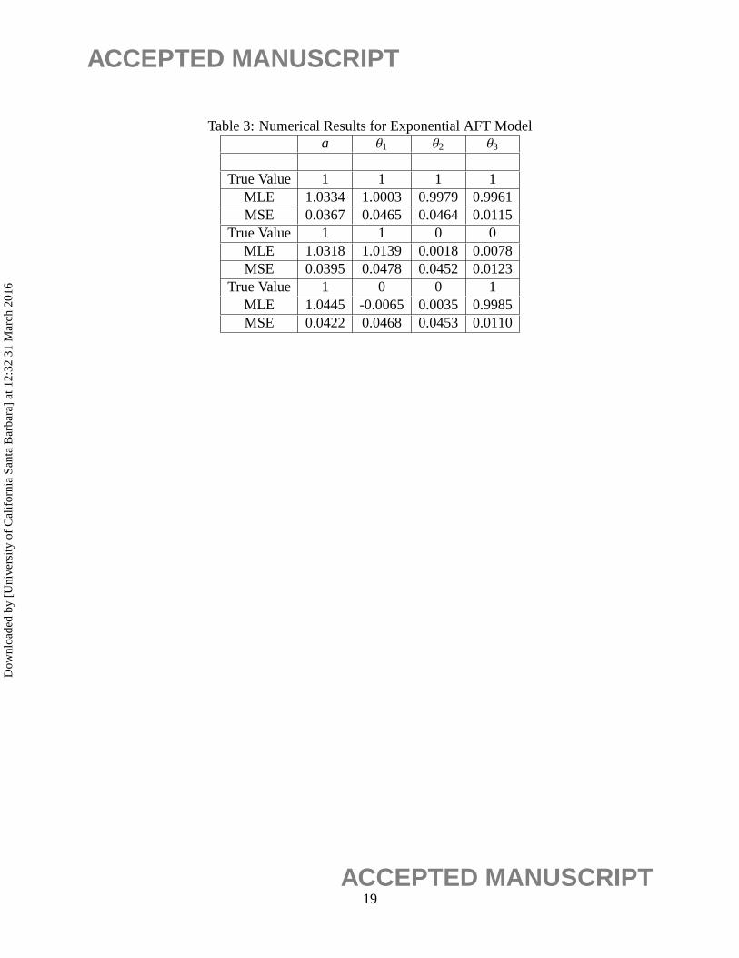
distribution. Similar to Pan (1999), three cases for the true covariate effects were considered. They

are θ = (1, 1, 1), θ = (1, 0, 0), andθ = (0, 0, 1). These three cases were chosen since they

represent the case where all covariates have an equal effect, where only one Bernoulli covariate

has an effect, and where only the Normally distributed covariate had an effect. In the exponential

case, between 7% to 36% of the observations were censored, between 9% and 42% in the case of

the Gamma distribution and between 8% and 40% in the Weibull case. Table 3, 4 and 5report the

results from these simulations. The MLE’s of all the parameters in all cases are very close to the

actual value, and the mean-squared errors are also small.

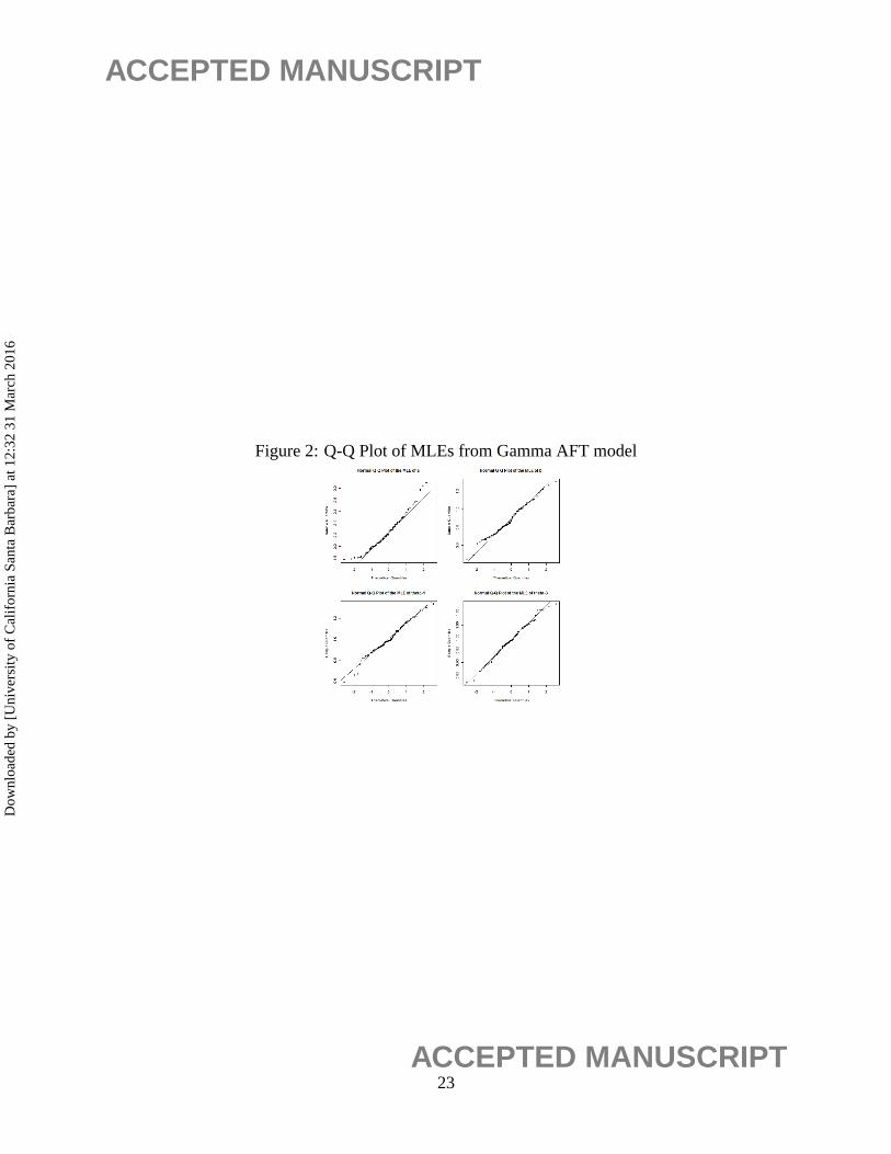
Finally we evaluate the theoretical convergence to normality of the estimators via simulations.

For this purpose, we simulateN = 100 samples of sizen = 100 each from the Gamma AFT and

Weibull AFT models described in the previous paragraph. We compute the MLEs for the samples

in the usual fashion. The Q-Q plots of the estimated values for the shape and scale parameters, and

first and third elements ofθ are displayed in Figures 2 and 3. These plots seem to indicate a fairly

good fit to normality.

5 Data Analysis

To highlight the usefulness of the methods developed in the previous sections, we will now consider

a dataset from Environmental Economics. The data studied is from a Contingent Valuation study

conducted by Cecilia Hakansson from Sweden and Katja Parkkila from Finland in 2004. People

in Finland were asked how much they were willing-to-pay (WTP) to increase the salmon stock in

a particular river basin. Participants were allowed to either give an exact amount that they were

WTP or provide an interval which contained their WTP if they preferred.

A total of 205 Finnish subjects provided data for their WTP and income. Of the 205 responders,

57 gave intervals, thus 27.8% of the data is middle censored. We fit a Weibull AFT model to this

data, using equation (24) with 1 covariate. The fitted values for this are: ˆa = 1.4407,b̂ = 0.0149,

θ̂ = −0.1610. To transform the parameter value onto the WTP scale, we must look at exp[θ̂]=

13ACCEPTED MANUSCRIPT

Dow

nloa

ded

by [

Uni

vers

ity o

f C

alif

orni

a Sa

nta

Bar

bara

] at

12:

32 3

1 M

arch

201

6

ACCEPTED MANUSCRIPT

0.8513. In this dataset, this means that people with higher incomes have a lower WTP.

6 Conclusion

In conclusion, we prove that the maximum likelihood estimates from a large family of distribu-

tions will converge in the case of middle censoring, and we give their large sample properties.

Additionally, we also consider the case of parametric models with the presence of covariates and

again provide the large sample properties of these estimators. In both cases, simulation studies are

presented illustrating the usefulness and accuracy of these methods.

The MLE’s of the regression coefficients are very close to the true value in all cases, but the

MLE’s of the parameters from the Gamma distribution are slightly off. Again, in all cases, the

mean-squared errors are small for all parameters except for ˆaMLE. Table 5 reports the results from

these simulations. The MLE’s of the regression coefficients are very close to the true value in the

case of equal effects of all covariates, but the estimates are slightly when only one covariate has an

effect. The MLE’s of the parameters from the Weibull distribution are fairly good, but ˆaMLE was

consistently underestimated. Again, in all cases, the mean-squared errors are quite small for all the

parameters, demonstrating that the estimation procedures work well. Finally, this methodology is

very flexible and applicable to many different areas of research, as demonstrated by the Contingent

Valuation example.

14ACCEPTED MANUSCRIPT

Dow

nloa

ded

by [

Uni

vers

ity o

f C

alif

orni

a Sa

nta

Bar

bara

] at

12:

32 3

1 M

arch

201

6

ACCEPTED MANUSCRIPT

References

[1] Dempster, A. P., Laird, N. M., and Rubin, D. B., (1997), Maximum likelihood from

incomplete data via the EM algorithm,Journal of the Royal Statistical Society, Series B,

39, 1–22.

[2] Gentleman, R. and Geyer, C.J., (1994), Maximum likelihood for interval censored data:

Consistency and computation,Biometrika, 81, 618–623.

[3] Iyer, S. K., Jammalamadaka, S. Rao, and Kundu, D. (2008), Analysis of Middle-Censored

Data with Exponential Lifetime Distributions,Journal of Statistical Planning and Infer-

ence, 138, No. 11, 3550–3560.

[4] Jammalamadaka, S. Rao, and Mangalam, V. (2003), Nonparametric estimation for middle

censored data,Journal of Nonparametric Statistics,15, No.2, 253–265.

[5] Jammalamadaka, S. Rao, and Mangalam, V. (2009), A general censoring scheme for

circular data,Statistical Methodology, 15, No. 3, 280–289.

[6] Keiding, N., Andersen, P. K., and Klein, J. P. (1997), The Role of Frailty Models and Ac-

celerated Failure Time Models in Describing Heterogeneity Due to Omitted Covariates,

Statistics in Medicine, 16, (1-3), 215–224.

[7] Kundu, D., and Pradhan, B. (2014), Analysis of Interval-Censored Data with Weibull

Lifetime Distribution,Sankhya B, 76, No. 1, pp 120-139.

[8] Lawless, J.F., (2003),Statistical models and methods for lifetime data, 2nd Ed., John

Wiley & Sons, New York.

[9] Tsai, W.Y. and Crowley, J., (1985), A large sample study of generalized maximum like-

lihood estimators from incomplete data via self-consistency,The Annals of Statistics, 13,

4, 1317–1334.

15ACCEPTED MANUSCRIPT

Dow

nloa

ded

by [

Uni

vers

ity o

f C

alif

orni

a Sa

nta

Bar

bara

] at

12:

32 3

1 M

arch

201

6

ACCEPTED MANUSCRIPT

[10] Wei, P. (1999), Extending the Iterative Convex Minorant Algorithm to the Cox Model

for Interval-Censored Data,Journal of Computational and Graphical Statistics, 8, No. 1,

109-120.

[11] Wu, C.F.J. (1983), On the Convergence Properties of the EM Algorithm,The Annals of

Statistics, 11, 95–103.

16ACCEPTED MANUSCRIPT

Dow

nloa

ded

by [

Uni

vers

ity o

f C

alif

orni

a Sa

nta

Bar

bara

] at

12:

32 3

1 M

arch

201

6

ACCEPTED MANUSCRIPT

Table 1: Numerical Results for Gamma(a = 2, b = 1) Lifetimes(α, β) (1, 1) (0.5,0.5) (0.5,1) (1.25,0.75)

n50 a est 2.1150 2.0914 2.1245 2.1062

b est 0.9980 0.9982 0.9757 0.9880MSE a 0.2084 0.1805 0.2064 0.1868MSE b 0.0453 0.0479 0.0479 0.0438

Censored (0.08,0.44) (0.04,0.50) (0.04,0.44) (0.14,0.50)100 a est 2.0676 2.0665 2.0534 2.0562

b est 0.9882 0.9814 0.9935 0.9959MSE a 0.0962 0.0904 0.0856 0.0944MSE b 0.0239 0.0237 0.0232 0.0255

Censored (0.13,0.40) (0.13,0.43) (0.08,0.31) (0.20,0.47)500 a est 2.0144 2.0135 2.0013 2.010

b est 0.9960 0.9963 0.9968 0.9989MSE a 0.0153 0.0159 0.0147 0.0168MSE b 0.0046 0.0049 0.0045 0.0050

Censored (0.19,0.33) (0.23,0.36) (0.14,0.25) (0.25,0.39)

17ACCEPTED MANUSCRIPT

Dow

nloa

ded

by [

Uni

vers

ity o

f C

alif

orni

a Sa

nta

Bar

bara

] at

12:

32 3

1 M

arch

201

6

ACCEPTED MANUSCRIPT

Table 2: Numerical Results for Weibull(a = 2, b = 1) Lifetimes(α, β) (1, 1) (0.5,0.5) (0.5,1) (1.25,0.75)

n50 a est 1.9273 1.9635 1.9659 1.8799

b est 1.1211 1.1504 1.1000 1.1569MSE a 0.0952 0.0905 0.0667 0.1172MSE b 0.0716 0.0730 0.0500 0.1038

Censored (0.12,0.54) (0.10,0.44) (0.06,0.40) (0.16,0.60)100 a est 2.0275 2.0305 2.0417 1.9930

b est 1.1015 1.1386 1.0859 1.1193MSE a 0.0107 0.0098 0.0102 0.0160MSE b 0.0391 0.0416 0.0224 0.0508

Censored (0.19,0.47) (0.14,0.39) (0.10,0.33) (0.22,0.56)500 a est 2.0008 2.0024 2.0042 2.0002

b est 1.0414 1.1032 1.0468 1.0639MSE a 0.00016 0.00048 0.00084 0.00004MSE b 0.01076 0.02344 0.01040 0.02004

Censored (0.26,0.39) (0.19,0.32) (0.15,0.26) (0.34,0.47)

18ACCEPTED MANUSCRIPT

Dow

nloa

ded

by [

Uni

vers

ity o

f C

alif

orni

a Sa

nta

Bar

bara

] at

12:

32 3

1 M

arch

201

6

ACCEPTED MANUSCRIPT

Table 3: Numerical Results for Exponential AFT Modela θ1 θ2 θ3

True Value 1 1 1 1MLE 1.0334 1.0003 0.9979 0.9961MSE 0.0367 0.0465 0.0464 0.0115

True Value 1 1 0 0MLE 1.0318 1.0139 0.0018 0.0078MSE 0.0395 0.0478 0.0452 0.0123

True Value 1 0 0 1MLE 1.0445 -0.0065 0.0035 0.9985MSE 0.0422 0.0468 0.0453 0.0110

19ACCEPTED MANUSCRIPT

Dow

nloa

ded

by [

Uni

vers

ity o

f C

alif

orni

a Sa

nta

Bar

bara

] at

12:

32 3

1 M

arch

201

6

ACCEPTED MANUSCRIPT

Table 4: Numerical Results for Gamma AFT Modela b θ1 θ2 θ3

True Value 2 1 1 1 1MLE 2.2761 0.8961 1.0005 1.0021 1.0012MSE 0.1927 0.0415 0.0238 0.0227 0.0057

True Value 2 1 1 0 0MLE 2.3025 0.8842 1.0102 -0.0092 0.0009MSE 0.2146 0.0421 0.0225 0.0236 0.0058

True Value 2 1 0 0 1MLE 2.2383 0.9166 0.0022 0.0115 0.9986MSE 0.1641 0.0377 0.0230 0.0208 0.0060

20ACCEPTED MANUSCRIPT

Dow

nloa

ded

by [

Uni

vers

ity o

f C

alif

orni

a Sa

nta

Bar

bara

] at

12:

32 3

1 M

arch

201

6

ACCEPTED MANUSCRIPT

Table 5: Numerical Results for Weibull AFT Modela b θ1 θ2 θ3

True Value 2 1 1 1 1MLE 1.8582 1.0556 1.0452 1.0579 1.0502MSE 0.0303 0.0411 0.0190 0.0218 0.0081

True Value 2 1 1 0 0MLE 1.9251 1.0796 1.1554 -0.0094 0.0040MSE 0.0197 0.0470 0.0431 0.0245 0.0066

True Value 2 1 0 0 1MLE 1.8714 0.9847 -0.0136 0.0008 1.1471MSE 0.0277 0.0457 0.0319 0.0319 0.0275

21ACCEPTED MANUSCRIPT

Dow

nloa

ded

by [

Uni

vers

ity o

f C

alif

orni

a Sa

nta

Bar

bara

] at

12:

32 3

1 M

arch

201

6

ACCEPTED MANUSCRIPT

Figure 1: Goodness of Fit using the Gamma distribution

22ACCEPTED MANUSCRIPT

Dow

nloa

ded

by [

Uni

vers

ity o

f C

alif

orni

a Sa

nta

Bar

bara

] at

12:

32 3

1 M

arch

201

6

ACCEPTED MANUSCRIPT

Figure 2: Q-Q Plot of MLEs from Gamma AFT model

23ACCEPTED MANUSCRIPT

Dow

nloa

ded

by [

Uni

vers

ity o

f C

alif

orni

a Sa

nta

Bar

bara

] at

12:

32 3

1 M

arch

201

6

ACCEPTED MANUSCRIPT

Figure 3: Q-Q Plot of MLEs from Weibull AFT model

24ACCEPTED MANUSCRIPT

Dow

nloa

ded

by [

Uni

vers

ity o

f C

alif

orni

a Sa

nta

Bar

bara

] at

12:

32 3

1 M

arch

201

6