preschool and maternal labor market outcomes:...

� 2011 by The University of Chicago. All rights reserved. 0013-0079/2011/5902-0001$10.00

Preschool and Maternal Labor Market Outcomes:Evidence from a Regression Discontinuity Design

samuel berlinskiUniversity College London and Institute for Fiscal Studies

sebastian galianiWashington University in St. Louis

patrick j. mc ewanWellesley College

I. IntroductionAfter World War II, female labor participation rates rose steadily in thedeveloped and developing world. However, participation rates in many coun-tries are still relatively low for mothers with young children. Not surprisingly,expanding preschool education is an often-cited goal in both developed coun-tries (OECD 2002) and Latin America (Myers 1995; Schady 2006). It providesan implicit child care subsidy, while also, perhaps, improving child outcomes(Blau and Currie 2006). While a subsidy specifically designed to achieve oneof these goals will usually be relatively ineffective at accomplishing the othergoal, the hope is that free public preschool could attain both. Nonetheless,the empirical evidence on the effects of preprimary education is still limited,especially for developing countries.1

In two pertinent examples from South America, Berlinski, Galiani, andGertler (2009) find a positive effect of preprimary school attendance on theSpanish and mathematics test scores of Argentine third graders, as well asbehavioral outcomes such as attention, effort, class participation, and discipline.Berlinski, Galiani, and Manacorda (2008), using data from the Uruguayan

We thank Joseph Shapiro for his contributions to the article. We further thank Phil Levine, CostasMeghir, Stephen Nickell, Imran Rasul, and the referees and editors for their useful suggestions.Samuel Berlinski gratefully acknowledges financial help from the ESRC-DFID grant RES-167-25-0124. Please contact the corresponding author, Patrick J. McEwan, at [email protected] There is empirical evidence from the United States that intensive early education interventionstargeted specifically to disadvantaged children yield benefits in the short and in the long run (Blauand Currie 2006). On the less extensive evidence in Latin America, see Schady (2006).

314 economic development and cultural change

household survey that collects retrospective information on preschool atten-dance, find small gains in school attainment from preschool attendance thatare magnified with age. We know less about the effects of preschool on maternallabor market outcomes.

A major impediment to identifying the causal effect of preprimary schoolattendance on child or parent outcomes is nonrandom selection into earlyeducation. In Argentina, the school year runs from March to December, andenrollment in the final year of preschool is mandatory for children who turn5 years old by June 30. Children born on July 1 must wait 1 year to enrollin kindergarten. Using pooled household surveys that report exact birth dates,we confirm that children born on July 1 have sharply lower probabilities, byabout 0.3, of attending school. We exploit this plausibly exogenous variationin the probability of attendance to identify the effect of early school attendanceon maternal labor market outcomes.

The parameters we study, however, differ from those of much research inthe child-care and female labor supply literature. Although many studies haveestimated the sensitivity of maternal employment to costs of child care, theirelasticity estimates cannot be easily generalized to predict the effects of ex-panding preschool education on maternal labor market outcomes (Andersonand Levine 2000; Blau and Currie 2006).2 Additionally, in the absence ofcredible instruments, identification of the elasticities of maternal employmentto child-care costs is challenging (Browning 1992).

Our regression-discontinuity estimates suggest that, on average, 13 mothersstart to work for every 100 youngest children in the household that startpreschool (although, in our preferred specification, this estimate is not statis-tically significant at conventional levels). Furthermore, mothers are 19.1 per-centage points more likely to work for more than 20 hours a week (i.e., moretime than their children spend in school) and to work, on average, 7.8 morehours per week as a consequence of their youngest offspring attending pre-school. We find no effect of preschool attendance on maternal labor outcomesfor children who are not the youngest in the household. Finally, we find thatat the point of transition from kindergarten to primary school there are per-sistent employment effects, even though school attendance is nearly universal.This might be explained by the fact that finding jobs takes time or by amother’s decision to work once the youngest child transitions to primaryschool.

2 For the mothers who would work fewer hours than the school day, public schools provide a100% marginal price subsidy for child care of fixed quality, while for the mothers who wouldotherwise work more hours the price subsidy is inframarginal (Gelbach 2002).

Berlinski, Galiani, and McEwan 315

Our preferred estimates condition on mother’s schooling and other exog-enous covariates, given evidence that mothers’ schooling is unbalanced in thevicinity of the July 1 cutoff in the sample of 4-year-olds. Using a large setof natality records, we find no evidence that this is due to precise birth datemanipulation by parents. Other explanations, like sample selection, are alsonot fully consistent with the data.

Our empirical strategy is related to work in the United States by Gelbach(2002), Barua (2007), and Fitzpatrick (2008). Gelbach estimates the effect ofpublic school enrollment of 5-year-old children on their mothers’ labor marketoutcomes, using U.S. census data and instrumenting enrollment with quarter-of-birth dummy variables. He finds that free public school enrollment increaseslabor supply measures by 6%–24% among women whose youngest child is5. Barua (2007) finds similar effects, but concentrated among married womenwhose youngest child is 5. Using more recent data with exact birth dates,Fitzpatrick (2008) finds that universal prekindergarten in some states doesnot increase the labor supply of most women.

Related literature from several countries reports difference-in-differencesestimates of preschool effects on maternal labor market outcomes, relying ongeographic and temporal variation in policies that affect preschool attendance.3

Of particular relevance to this study’s findings, Berlinski and Galiani (2007)examine an Argentine infrastructure program, initiated in 1993, that builtpreprimary classrooms for children aged 3–5. Using the fact that the con-struction exhibited variation in its intensity across provinces, difference-in-differences estimates suggest that the take-up of new preschool vacancies isperfect. The estimates further suggest that when a child is exogenously inducedto attend preschool by the supply expansion, the likelihood of maternal em-ployment increases between 7 and 14 percentage points, roughly similar tothis study’s point estimates. However, Berlinski and Galiani only find a small,imprecisely estimated effect on hours worked.

The rest of the article is organized as follows. Section II provides backgroundinformation on the education system in Argentina and describes the data sets

3 Cascio (2009) exploits variation across the United States in the funding of kindergarten initiativesin the late 1960s and early 1970s. She finds positive effects of kindergarten enrollment on maternallabor supply for single mothers of 5-year-olds with no younger children. Baker, Gruber, and Milligan(2008) study the expansion of subsidized provision of child care for children 0–4 in the Canadianprovince of Quebec. They also find that child care use has a positive effect on maternal labor supplyfor married mothers. Finally, Schlosser (2006) studies the impact on labor supply of the gradualimplementation of compulsory preschool laws for children aged 3–4 in Israel. She also finds thatthe provision of preschool education in Arab towns increases enrollment and maternal labor supply.


used in this study. Section III describes our identification strategy. Section IVreports the empirical results, and Section V concludes.

II. Background and DataA. Background InformationArgentina is a middle-income developing country with a long tradition offree public schooling. The school system is divided into preprimary, primary,and secondary education. Primary school attendance between 6 and 12 yearsold is virtually universal. However, the preprimary attendance rate amongchildren aged 3–5 years old was only 64% in 2001 (Berlinski and Galiani2007). Preprimary education is divided into three levels: level 1 (age 3), level2 (age 4), and level 3 (age 5). In general, preprimary classes are held withinexisting primary schools. Like primary schools, they typically operate in sep-arate morning and afternoon shifts, with children attending one of these shiftsfor three and a half hours a day, 5 days a week, during a 9-month school year.

Primary school has been compulsory since 1885. The Federal EducationLaw of 1993 further mandated attendance between level 3 of preprimaryeducation and the second year of secondary school. Its implementation was tohave occurred gradually between 1995 and 1999, but it was not rigidlyenforced. First, there is no penalty in place for noncompliers. Second, primaryschool enrollment is not impeded by lack of preprimary schooling. Finally,there are still large dropout rates at ages 13 and older.

In Argentina, the academic school year starts early in March and finishesin December. Like many countries, a cutoff date establishes who can enrollin a given academic year. School age is defined by the age attained on June30 of the current academic year.4 Children can enroll in level 3 of preschoolif they turn 5 years old on or before June 30 of the current school year.

Until 1994 Argentina was a relatively low unemployment country withunemployment rates never exceeding 10%. However, unemployment increasedsubstantially after a macroeconomic shock in 1995 with an average rate of14.5 for the rest of the nineties. High unemployment might tend to attenuatethe impact of preschool attendance on maternal labor outcomes. Annual hoursworked are high, and female participation is at the level of southern Europe.In 1998, the female employment rate for the group aged 18–49 was 48%.

The Argentine labor market is not very rigid. Tax rates in Argentina arecomparable to those in a typical non-European OECD country. Unions are animportant feature of economic life, with around half the workers having theirwages bargained collectively and 45% of employees being union members.

4 See, e.g., Article 39, Resolucion CABA: No. 626/1980.


However, national minimum wages are set at a relatively low level and probablydo not have much impact on employment. Finally, employment protection isat about the average OECD level (Galiani and Nickell 1999).

B. DataWe use data from the Argentine household survey, the Encuesta Permanentede Hogares (EPH), a biannual survey of about 100,000 households managedby Argentina’s National Institute of Statistics and Censuses (INDEC). Thesurvey is representative of the urban population of Argentina (approximately90% of the population resides in urban areas). It has been conducted since1974 in the main urban clusters (referred to as agglomerates) of each provinceof the country, with the exception of Rio Negro.5 A unique feature of thishousehold survey is that from May 1995 to May 2003 it includes the exactdate of birth for each individual in the sample. We pool repeated cross-sectionsof individual-level data from both waves of the survey covering the 1995–2001 period. We do not use the information for 2002 onward because of themacroeconomic collapse of 2002 and its economic and distributional conse-quences (Mussa 2002; Galiani, Heymann, and Tommasi 2003).6

For our main results, we use a sample of households including mothersbetween the ages of 18 and 49 and at least one child aged 4 on January 1 ofthe survey year. The survey collects information on the family relationshipbetween household members and the head of household. Our analysis is limitedto children of either male or female household heads, because only in suchcases can the mother of a child be identified in the EPH. We further restrictthe sample to individuals with full information on date of birth, school at-tendance, mother’s age and education, and siblings’ ages. When children ofthe same household are born on the same day we only include one of thechildren in the household.

In the first panel of table 1 we summarize the information contained inthe EPH sample. On average, 58% of children aged 4 on January 1 of thesurvey year attended school. However, the enrollment rate was 82% for thoseborn in the first half of the year and 33% for those born on or after July 1.Thirty-seven percent of the mothers worked the previous week, with 30%working 20 or more hours per week (i.e., more time than their children spendin school). The average number of hours worked last week is 12.17. The

5 Urban Rio Negro was included in the survey in 2001. See www.indec.gov.ar for detailed infor-mation on the EPH.6 GDP declined 20% and unemployment peaked at 24%. The results using the 1995–2003 sampleare similar to although less precise than those reported here and are available from the authorsupon request.

318

TAB

LE1

VA

RIA

BLE

DE

FIN

ITIO

NS

AN

DD

ESC

RIP

TIV

EST

ATI

STIC

S

Mea

n(S

tand

ard

Dev

iati

on)

Defi

niti

on

All

Bir

thd

ays

6/30

or

Ear

lier

Bir

thd

ays

on

7/1

or

Late

rM

inim

um/M

axim

umN

A.

Enc

uest

aP

erm

anen

ted

eH

og

ares

,M

ay19

95to

Oct

ob

er20

01(4

-Yea

r-O

lds)

Bir

thd

ayC

hild

’sd

ayo

fb

irth

inth

eca

lend

arye

ar,

defi

ned

toad

dre

ssle

apye

ars:

1/1

p

�18

2;7/

1p

0;12

/31

p18

3�

.40

�92

.30

91.2

1�

182/

183

22,9

74(1

05.9

2)(5

2.63

)(5

3.21

)B

orn

on/

afte

rcu

toff

Chi

ld’s

day

of

bir

this

7/1

or

late

r.5

00

10/

122

,974

Att

end

ssc

hoo

lC

hild

atte

nded

any

leve

lof

scho

ola

tti

me

of

surv

ey.5

8.8

2.3

30/

122

,974

Fem

ale

Chi

ldis

fem

ale

.48

.48

.49

0/1

22,9

74M

oth

er’s

age

Mo

ther

’sag

ein

dec

imal

year

s32

.81

33.0

432

.58

18.0

1/49

.94

22,9

74(6

.24)

(6.2

4)(6

.23)

Mo

ther

’ssc

hoo

ling

Mo

ther

’sye

ars

of

form

alsc

hoo

ling

9.37

9.35

9.40

0/17

22,9

74(3

.90)

(3.8

6)(3

.94)

Mo

ther

wo

rks

Mo

ther

wo

rked

last

wee

k.3

7.3

7.3

70/

122

,974

Mo

ther

wo

rks

full

tim

eM

oth

erw

ork

ed20

or

mo

reho

urs

last

wee

k.3

0.3

0.3

00/

122

,841

Ho

urs

wo

rked

Mo

ther

’sho

urs

wo

rked

inal

ljo

bs

last

wee

k12

.17

12.0

712

.27

0/84

22,8

41(1

9.05

)(1

9.03

)(1

9.06

)

319

B.

Nat

alit

yFi

les,

2002

–5

Bir

thd

aySa

me

asab

ove

�.1

4�

45.4

545

.78

�91

/91

888,

033

(53.

18)

(26.

24)

(26.

72)

Bo

rno

n/af

ter

cuto

ffSa

me

asab

ove

.50

01

0/1

888,

033

Satu

rday

Bo

rno

nSa

turd

ay.1

2.1

2.1

20/

188

8,03

3Su

nday

Bo

rno

nSu

nday

.10

.10

.10

0/1

888,

033

Ho

liday

Bo

rno

na

nonfl

oat

ing

holid

ay:

5/1,

5/25

,7/

9.0

1.0

2.0

10/

188

8,03

3M

oth

er’s

age

Mo

ther

’sag

ein

inte

ger

year

s26

.37

26.4

126

.314

/45

888,

033

(6.5

0)(6

.50)

(6.5

0)M

oth

er’s

scho

olin

gM

oth

er’s

year

so

ffo

rmal

scho

olin

g9.

369.

339.

400/

1687

4,90

4(3

.84)

(3.8

4)(3

.84)

Low

birt

hwei

ght

Bir

thw

eig

htis

less

than

2,50

0g

ram

s.0

7.0

7.0

70/

187

7,55

1G

esta

tio

nW

eeks

of

ges

tati

on

38.7

838

.78

38.7

714

/45

857,

330

(1.8

9)(1

.89)

(1.8

9)P

ublic

faci

lity

Chi

ldb

orn

ina

pub

liche

alth

faci

lity

.58

.59

.58

0/1

886,

909

Live

sw

ith

par

tner

Mo

ther

lives

wit

ha

par

tner

.84

.84

.84

0/1

864,

879

No

te.

The

Enc

uest

aP

erm

anen

ted

eH

og

ares

sam

ple

(pan

elA

)in

clud

esch

ildre

nfr

om

surv

eys

bet

wee

nM

ay19

95an

dO

cto

ber

2001

who

wer

e4

year

so

ldo

nJa

nuar

y1

of

the

surv

eyye

aran

dha

da

mo

ther

pre

sent

aged

18–4

9.Th

ena

talit

yfil

es(p

anel

B)

incl

ude

bir

ths

fro

mth

e20

02–5

files

,of

mo

ther

sag

ed14

–45

that

occ

urre

db

etw

een

Ap

ril

1an

dSe

pte

mb

er30

.


employment rate for the mothers of children who attend preschool is 38%,versus 35% for those who do not. On average, maternal characteristics suchas age, education, and labor market outcomes for the mothers of children bornin each half of the year are statistically similar.

We also use natality data from birth certificates, compiled by Argentina’sMinistry of Health.7 It is not compulsory for provinces to report exact dateof birth, but—with the exception of the Province of Buenos Aires—all otherprovinces provide this information for the period 2002–5.8 From this data weextracted all births to mothers aged 14–45 (i.e., those who will be 18–49when their children turn 4). In the second panel of table 1 we summarize theinformation contained in the natality records.

III. Empirical StrategyThis section describes the regression-discontinuity approach that we use toidentify the effect of preschool attendance on maternal labor market outcomes.It exploits sharp differences in the probability of attendance for young childrenborn on either June 30 or July 1. As a starting point, consider the followinglinear model for a child aged 4 on January 1 of the survey year (i.e., a childwho is going to turn 5 in the calendar and academic year of the survey):

′Y p aS � b X � l � m � e , (1)ijs ijs ijs j s ijs

where is a labor market outcome for the mother of child i, residing inYijs

region j, and observed in survey round s (each survey round is the interactionof year and wave of the survey); is a dummy variable indicating schoolSijs

attendance; is a vector of covariates that affect maternal labor marketXijs

outcomes; and is an error term assumed to be independent and identicallyeijs

distributed. The model includes fixed effects for regions ( ), equivalent tolj

survey “agglomerates,” and survey rounds ( ). The parameter of interest, ,m as

represents the mean effect of a child’s preschool attendance on the maternallabor market outcome.9 Because the effects of preschool attendance on maternallabor outcomes could differ between households whose youngest child enterskindergarten with respect to those who have younger children we estimateseparate models and parameters for these groups.

If we estimate the model in equation (1) by ordinary least squares (OLS),the estimator of a is likely to be inconsistent. First, maternal labor market

7 Further information can be found at the Direccion de Estadısticas e Informacion de Salud Website: http://www.deis.gov.ar/.8 Natality data before 2002 do not contain exact date of birth.9 In the case of dichotomous measures of labor market outcomes, we also apply OLS and interpretcoefficient estimates as marginal probabilities.


outcomes and child’s school attendance are jointly determined, rendering theOLS estimator inconsistent. Second, omitted variables such as a mother’s cog-nitive ability are plausibly correlated with both labor outcomes and children’skindergarten attendance.

To disentangle the causal effect of preschool attendance, we use an instru-ment that induces plausibly exogenous variation in but has no direct effectSijs

on . In Argentina, children must turn 5 years old on or before June 30 ofYijs

the school year in which they enroll in (compulsory) kindergarten. Those bornone day later must wait a full year to enroll. Define a variable that indicatesBijs

a child’s day of birth during the calendar year. It equals �182 on January 1,0 on July 1, and 183 on December 31. Further define , anZ p 1{B ≥ 0}ijs ijs

indicator function that equals to one for children born on or after July 1, andzero otherwise.

We model school attendance using a linear probability model:2S p d Z � d B � d B � d Z # B �ijs 0 ijs 1 ijs 2 ijs 3 ijs ijs (2)

2d Z # B � l � m � u .4 ijs ijs j s ijs

The parameter measures the discontinuity in preschool attendance on Julyd0

1. In our sample of Argentine 4-year-olds, we anticipate that , sinced ! 00

children born on or after July 1 do not fulfill the minimum age requirementfor enrollment in kindergarten. In practice, the point estimate is likely to begreater than �1 (a so-called “fuzzy” discontinuity), since younger childrenmay already be enrolled in the previous, noncompulsory level of preschool,and some older children may ignore compulsory attendance rules.

Similarly, we can model maternal labor market outcomes as2Y p a Z � a B � a B � a Z # B �ijs 0 ijs 1 ijs 2 ijs 3 ijs ijs (3)

2a Z # B � l � m � h ,4 ijs ijs j s ijs

where captures the reduced-form effect of July 1 birthdays on labor out-a0

comes. Since we anticipate that , the estimate of a0 must be rescaledd 1 �10

by the estimate of to recover the effect of school attendance on labord0

outcomes. In practical terms, this parameter is computed by estimating equa-tion (1) via two-stage least squares (TSLS), conditioning on the interactedpolynomials of in both stages, and instrumenting with (see, e.g.,B S Zijs ijs ijs

Hahn, Todd, and van der Klaauw 2001; van der Klaauw 2002; Imbens andLemiuex 2008).

For this strategy to identify the parameter of interest, must be correlatedZijs

with , but it should not have a direct effect on the outcome of interest,Sijs

that is, . Since parents can time conception, a child’s seasonCov (Z , e ) p 0ijs ijs


of birth is plausibly correlated with unobserved variables like child health andfamily income, any of which could directly influence maternal labor marketoutcomes (Bound, Jaeger, and Baker 1995; Bound and Jaeger 2000). To addressthis, the TSLS specifications control for smooth functions of , estimatedBijs

separately on either side of the cutoff date.10 The specification above assumesa piecewise quadratic polynomial, but we verify it through visual inspectionof means taken within day-of-birth cells, in addition to reporting estimateswith higher-order polynomials.

Although the polynomials capture smooth, seasonal differences in birth datemanipulation, they cannot capture precise manipulation, near the cutoff date,via caesarean sections or induced births. In the next section, we use natalitydata from birth certificates to show that this is an unlikely source of bias.Another possible threat to the internal validity of our estimates could comefrom welfare subsidies varying with school age. In this scenario, we couldconfound the effect of preschool attendance with the effect of these subsidies.To our knowledge, in Argentina, no such overlapping discontinuities exist inthe design of the welfare system. Finally, parents may deceive educationalauthorities about their child’s date of birth in order to enroll them in preschoolearlier. This practice is difficult to implement in Argentina, since enrollmentrequires a national identification card that includes the officially recorded dateof birth. Moreover, this would only constitute a threat to internal validity ifparents lie to the household survey about birth dates (in addition to the schoolauthorities), which they have no incentive to do.

The interpretation of the TSLS estimates requires some clarification.11 Undera weak monotonicity assumption, as in Imbens and Angrist (1994), the es-timates are informative about the behavior of compliers (i.e., the subgroup ofindividuals whose treatment status switches from nonrecipient to recipient iftheir birth date crosses the cutoff). Our analysis includes children who willturn 5 years old during the academic year. In this sample, the subgroup ofnoncompliers includes households that choose to send their children to pre-

10 The estimated regression functions do not fully saturate the model. Lee and Card (2008) showthat one can interpret the deviation between the true conditional expectation function and theestimated regression function as random specification error that introduces a group structure intothe standard errors for the estimated treatment effect. Thus, we always report standard errorsclustered by 366 days of birth.11 One interpretation for the parameters we estimate is that of an equivalent cash child care subsidy.We find this interpretation less straightforward as preschool education as a means of child careimposes fixed costs on parents (e.g., children have to be taken and collected from school at certaintimes) that a child care cash subsidy may not. Parents likely also value the learning of childrenduring preprimary education. Finally, the population that would be affected by these two conceptualexperiments might be different.


school for 2 years or more, and thus are not influenced by the cutoff date. Incontrast, the compliers include households that choose only 1 year of preschool.Thus, our estimates are most generalizable to households that choose lesspreschool, perhaps likely to be poorer and credit constrained, or with lessaccess to preschool infrastructure.

IV. Main ResultsA. Evidence on Precise Birth TimingWe investigate the validity of our identifying assumption by examiningwhether there is manipulation of the assignment variable, perhaps via caesareansection or induced labor.12 This is plausible in Argentina, where one-quarterof births are via caesarean section, with rates between 36% and 45% in privatehospitals (Belizan et al. 1999). Presuming that timed births do not occur froma random draw of the population, it is plausible that the clustering of suchparents just to the left (or right) of the July 1 cutoff could introduce acorrelation between and .Z eijs ijs

We use two strategies to diagnose precise manipulation of the assignmentvariable (Imbens and Lemieux 2008; Lee 2008). First, we examine the densityof birth dates around the July 1 cutoff for clustering on either side of thecutoff. Second, we examine the distribution of observed socioeconomic andbirth characteristics around the enrollment cutoff, interpreting sharp changesin these variables as suggestive of nonrandom birth date manipulation.

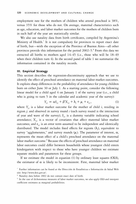
Figure 1 describes data on large samples of births from natality data. Thereis strong evidence that families are able to precisely time births (also seeMcEwan and Shapiro 2008). The upper-left panel shows proportionally fewerbirths on weekends, and that mothers of such births have less schooling. Thispattern, common across many countries, has been shown to be correlated withthe use of caesarean sections and induced labor (Dickert-Conlin and Chandra1999). To determine whether such birth timing might occur around July 1,the upper-right panel reports a histogram of all births. Because of the largesample, we restrict it to a 6-month window around July 1, but the resultsare robust to a larger window. While there are visible dips in births on threenational holidays, consistent with the ability to time births, there is no clearevidence of birth clustering on either side of the July 1 cutoff date.

12 In Chile, with a similarly high rate of caesarean sections (Belizan et al. 1999), there is no evidenceof birth timing around a July 1 enrollment cutoff (McEwan and Shapiro 2008). In the UnitedStates, McCrary and Royer (2006) find no evidence of sorting around birth date cutoffs in Texasand California. In other countries, evidence suggests that parents have manipulated birth dates inorder to avoid taxes (Dickert-Conlin and Chandra 1999) and obtain monetary bonuses (Gans andLeigh 2009).


Figure 1. Evidence of birth day sorting on natality records. In upper left, bars indicate the percent oftotal births, and dots indicate mean mother’s schooling. In upper right, black bars indicate the cutoff(7/1) and three nonfloating holidays (5/1, 5/25, and 7/9). In the bottom panels, dots indicate mean valueswithin day-of-birth cells, while solid dots indicate means on three nonfloating holidays, for weeks ofgestation (lower left) and mother’s schooling (lower right). Source: Natality records, 2002–5.

In the bottom panels of figure 1, we summarize the relationship betweenbirth dates and two variables: weeks of gestation and mother’s schooling. Thecircles represent the unadjusted means of these variables within daily cells.The superimposed lines are fitted values from a piecewise quadratic specifi-cation on date of birth. There is, interestingly, evidence that declines in birthfrequencies on holidays are associated with lower values of mothers’ schooling(indicated by the solid dots). However, there is no visual evidence of breaksaround July 1.

In table 2, we present OLS regression results that are the analogue of thevisual evidence in the bottom panels of figure 1. This table confirms thefinding of no differences in gestation and schooling near the July 1 cutoff. Itshows similar results for a larger set of covariates that include low birth weight.In sum, the natality data provide no evidence of precise manipulation of birthdates around the July 1 cutoff.

B. Day of Birth, Preschool Attendance, and Covariate SmoothnessWe turn now to the analysis of preschool attendance and covariate smoothnessusing the EPH sample. In figure 2, we summarize the relationship between

325

TAB

LE2

DA

YO

FB

IRTH

AN

DB

ASE

LIN

EV

AR

IAB

LES,

NA

TALI

TYD

ATA

Mo

ther

’sSc

hoo

ling

(1)

Mo

ther

’sA

ge

(2)

Low

Bir

thW

eig

ht(3

)G

esta

tio

n(4

)P

ublic

Faci

lity

(5)

Live

sw

ith

Par

tner

(6)

Bo

rno

n/af

ter

cuto

ff.0

22.0

87*

�.0

01.0

12�

.003

.001

(.025

)(.0

51)

(.002

)(.0

15)

(.004

)(.0

02)

Sund

ay�

.517

***

�.9

44**

*.0

06**

*.0

11.1

05**

*�

.025

***

(.019

)(.0

36)

(.001

)(.0

10)

(.003

)(.0

01)

Satu

rday

�.2

95**

*�

.633

***

.007

***

�.0

08.0

60**

*�

.018

***

(.019

)(.0

34)

(.001

)(.0

08)

(.003

)(.0

02)

Ho

liday

�.3

22**

*�

.377

***

.001

.026

**.0

53**

*�

.010

***

(.044

)(.0

75)

(.001

)(.0

11)

(.006

)(.0

03)

Co

ntro

ls?

Yes

Yes

Yes

Yes

Yes

Yes

Ob

serv

atio

ns87

4,90

488

8,03

387

7,55

185

7,33

088

6,90

986

4,87

9

Sour

ce.

Nat

alit

yre

cord

s,20

02–5

.N

ote

.O

LSre

gre

ssio

ns.

Ro

bus

tst

and

ard

erro

rs,

adju

sted

for

clus

teri

ngin

day

-of-

bir

thce

lls,a

rein

par

enth

eses

.Ad

dit

iona

lco

ntro

lsin

clud

ed

umm

ies

for

bir

thye

ar,p

rovi

nce

of

bir

th,a

ndd

ayo

fw

eek

of

bir

thd

ay(e

xclu

din

gM

ond

ay).

All

reg

ress

ions

incl

ude

ap

iece

wis

eq

uad

rati

cp

oly

nom

ialo

fbir

thd

ate.

Sam

ple

incl

udes

allo

bse

rvat

ions

form

oth

ers

14–4

5w

ith

nonm

issi

ngva

lues

of

dep

end

ent

vari

able

and

exac

tb

irth

dat

e,b

etw

een

Ap

ril1

and

Sep

tem

ber

30.

*In

dic

ates

stat

isti

cals

igni

fican

ceat

10%

.**

Ind

icat

esst

atis

tica

lsig

nific

ance

at5%

.**

*In

dic

ates

stat

isti

cals

igni

fican

ceat

1%.


Figure 2. School attendance and day of birth, by age group. Dots indicate means of a dummy variableindicating school attendance within day-of-birth cells. Solid lines show fitted values of piecewise quadraticpolynomials. Source: Encuesta Permanente de Hogares, 1995–2001.

birth date and preschool attendance. The top panels present results among 3-and 4-year-olds who are the youngest in the household, and the bottom panelsamong those who are not the youngest in the household. (In this and allsubsequent analyses, children’s age is calculated on January 1 of the surveyyear in which they are observed.) The circles represent unadjusted means ofthe school attendance variable within daily cells. The superimposed lines arefitted values from a piecewise quadratic specification.

Figure 2 shows, as expected, that preschool attendance is low among 3-year-olds. There is a small break in attendance, with children born on or justafter July 1 slightly less likely to attend than children born just before. Alarger break is evident among 4-year-olds, consistent with the fact that kin-dergarten (i.e., level 3 of preschool) is compulsory. Four-year-olds born on July1 are just below the minimum age requirement for kindergarten and mustdelay enrollment by 1 year, while 4-year-olds born on June 30 are eligible toenroll as the youngest kindergarteners.

Table 3 reports OLS estimates of equation (2), the empirical analogue offigure 2. Panel A presents the results for the youngest children in the householdand panel B the results for children who are not the youngest in the house-


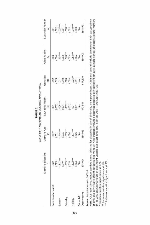
TABLE 3DAY OF BIRTH AND SCHOOL ATTENDANCE BY AGE GROUP

Dependent Variable: SchoolAttendance

(1) (2)

A. Youngest in household:3-year-olds �.048** �.057***

(.021) (.019)12,299 12,299

4-year-olds �.310*** �.299***(.029) (.029)10,990 10,990

B. Not youngest in household:3-year-olds �.052** �.071***

(.021) (.020)9,890 9,890

4-year-olds �.321*** �.331***(.027) (.026)11,984 11,984

Controls? No Yes

Source. Encuesta Permanente de Hogares, May 1995 to October 2001.Note. OLS regressions. Each cell reports the coefficient estimate of adummy variable indicating birthdays on or after July 1, based on eq. (2).Robust standard errors, adjusted for clustering in day-of-birth cells, arein parentheses. Controls include dummy variables for each survey round,sample cluster (agglomerate), day of week of birthday, and holiday birth-days (see text), in addition to linear and quadratic terms of mother’s age,a dummy variable indicating female children, and dummies for mother’syears of schooling.* Indicates statistical significance at 10%.** Indicates statistical significance at 5%.*** Indicates statistical significance at 1%.

hold.13 In column 1 of panel A, where we only condition on a piecewisequadratic polynomial, we find that among 4-year-olds, the coefficient on birth-days after June 30 is a large, negative, and highly significant estimate of�0.31. It is much smaller (�0.048) among 3-year-olds, albeit significant. Incolumn 2, we add a full set of controls, including dummy variables for eachsurvey round, regional agglomerate, day of week of birthday, birthdays onnonfloating holidays,14 linear and quadratic terms of mother’s age, a dummyvariable indicating female children, and dummies for mother’s years of school-ing. The results are not statistically different from those reported in column

13 A regression of a youngest in the household dummy on a born on/after July 1 dummy and apiecewise quadratic polynomial shows no correlation between being the youngest in the householdand the July 1 dummy.14 We include these variables to show that the results are not driven by coincidental overlap ofcutoff dates falling on weekends or holidays. Nevertheless, the results reported in this study arevery similar if we do not include these control variables.


TABLE 4DAY OF BIRTH AND BASELINE VARIABLES BY AGE GROUP

Dependent Variable

Female Mother’s Age Mother’s Schooling

(1) (2) (3) (4) (5) (6)

A. Youngest in Household

3-year-olds �.006 .001 �.017 .013 �.243 �.169(.036) (.036) (.479) (.483) (.266) (.260)

12,299 12,299 12,299 12,299 12,299 12,2994-year-olds .044 .050 �.105 �.052 �.810*** �.760***

(.034) (.033) (.466) (.464) (.232) (.222)10,990 10,990 10,990 10,990 10,990 10,990

B. Not Youngest in Household

3-year-olds �.039 �.039 .206 .175 �.065 �.086(.038) (.038) (.397) (.400) (.258) (.271)9,890 9,890 9,890 9,890 9,890 9,890

4-year-olds �.059* �.060* �.385 �.442 .004 �.096(.032) (.032) (.446) (.444) (.219) (.216)

11,984 11,984 11,984 11,984 11,984 11,984Controls? No Yes No Yes No Yes

Source. Encuesta Permanente de Hogares, May 1995 to October 2001.Note. OLS regressions. Each cell reports the coefficient estimate of a dummy variable indicating birth-days on or after July 1, based on eq. (3). Robust standard errors, adjusted for clustering in day-of-birthcells, are in parentheses. Controls include dummy variables for each survey round, sample cluster (ag-glomerate), day of week of birthday, and holiday birthdays (see text).* Indicates statistical significance at 10%.** Indicates statistical significance at 5%.*** Indicates statistical significance at 1%.

1, and the point estimates are very close in magnitude. The results for thesample of children who are not the youngest in the households are similar,suggesting that this aspect of family structure does not affect compliance withthe enrollment rule.

Before examining the effect of preschool attendance on maternal labor out-comes, we scrutinize whether, in the EPH sample, covariates are smooth aroundthe cutoff point. In table 4, we report successive OLS estimates of an equationlike (3) for mother’s age, years of schooling, and a dummy variable indicatingwhether the child is female. Panel A refers to the sample of children who arethe youngest in the household and panel B to the sample of children who arenot. The most obvious pattern is that mother’s schooling is systematicallylower among the youngest children in each household born on or after July1 (i.e., among children less likely to attend school). The basic result is robustto the inclusion of dummy variables for agglomerates, surveys, day of weekof birth, and holiday births. Interestingly, mother’s schooling is balancedaround the cutoff for the sample of children who are not the youngest in the


Figure 3. Mother’s schooling and day of birth, by age group. Dots indicate means of a variable indicatingyears of schooling within day-of-birth cells. Solid lines show fitted values of piecewise quadratic poly-nomials. Source: Encuesta Permanente de Hogares, 1995–2001.

household and for those children aged 3. In figure 3, we present the corre-sponding visual evidence for mother’s schooling.

In table 5, we present a number of robustness checks, both for the resultson preschool attendance and mother’s schooling. For brevity, we focus on thesample of 4-year-olds. We start by examining whether the quadratic specifi-cation is driving our results. Column 1 is the benchmark; for preschool at-tendance we reproduce the estimates of column 2 in table 3, with the full setof controls, and for mother’s schooling those of column 5 in table 4.15 Incolumns 2 and 3, we respectively include cubic and quartic piecewise poly-nomials. In the remaining columns, we use a piecewise quadratic polynomialbut within different samples. In column 4, we focus on the sample of childrenborn between April and September. In column 5, we drop a 1-week windowat both sides of the cutoff. In column 6, we use survey weights. None of thesechanges in the specification of the analysis affects the basic results we havepresented so far.

In the final two columns of table 5, we present the results of a placebo

15 The results for the mother’s schooling equations are similar if we include other controls anduse as the benchmark column 6 of table 4.

330

TAB

LE5

DA

YO

FB

IRTH

,SC

HO

OL

ATT

EN

DA

NC

E,

AN

DM

OTH

ER

’SSC

HO

OLI

NG

BY

AG

EG

RO

UP

:A

LTE

RN

ATI

VE

SPE

CIF

ICA

TIO

NS

AN

DSA

MP

LES

(1)

(2)

(3)

(4)

(5)

(6)

(7)

(8)

A.

4Ye

ars

Old

,Yo

ung

est

inH

ous

eho

ld

Att

end

scho

ol

�.2

99**

*�

.297

***

�.2

52**

*�

.274

***

�.2

91**

*�

.288

***

.014

�.0

14(.0

29)

(.038

)(.0

49)

(.039

)(.0

35)

(.048

)(.0

28)

(.035

)10

,990

10,9

9010

,990

5,45

410

,587

10,9

905,

286

5,70

4M

oth

er’s

scho

olin

g�

.810

***

�.8

53**

*�

.921

**�

.911

***

�.6

92**

�.8

36*

.503

�.0

47(.2

32)

(.313

)(.3

84)

(.330

)(.2

75)

(.476

)(.3

17)

(.400

)10

,990

10,9

9010

,990

5,45

410

,587

10,9

905,

286

5,69

9

B.

4Ye

ars

Old

,N

ot

Youn

ges

tin

Ho

useh

old

Att

end

scho

ol

�.3

31**

*�

.327

***

�.3

07**

*�

.302

***

�.3

38**

*�

.232

***

�.0

05.0

27(.0

26)

(.033

)(.0

42)

(.035

)(.0

32)

(.051

)(.0

33)

(.036

)11

,984

11,9

8411

,984

5,90

611

,515

11,9

846,

183

5,80

1M

oth

er’s

scho

olin

g.0

04�

.164

�.4

33�

.224

.233

.384

.161

�.2

08(.2

19)

(.259

)(.2

96)

(.264

)(.2

85)

(.332

)(.3

31)

(.297

)11

,984

11,9

8411

,984

5,90

611

,515

11,9

846,

183

5,80

1P

iece

wis

ep

oly

nom

ial

Qua

dra

tic

Cub

icQ

uart

icQ

uad

rati

cQ

uad

rati

cQ

uad

rati

cQ

uad

rati

cQ

uad

rati

cSa

mp

leFu

llFu

llFu

llB

orn

Ap

ril–

Sep

tem

ber

Bo

rn7/

1–7

and

6/24

–30

excl

uded

Full

with

surv

eyw

eig

hts

Bo

rn12

/1–6

/30

Bo

rn7/

1–12

/31

Sour

ce.

Enc

uest

aP

erm

anen

ted

eH

og

ares

,M

ay19

95to

Oct

ob

er20

01.

No

te.

The

“Ful

l”sa

mp

lean

des

timat

esfr

om(1

)are

bas

edon

tab

les

3an

d4,

cols

.2an

d5,

resp

ectiv

ely.

Inco

l.7,

the

dat

eof

birt

hva

riab

leis

cent

ered

onA

pril

1,an

dw

ere

por

tco

effic

ient

ofa

dum

my

equa

lto

1if

bor

non

Ap

ril1

oraf

ter

and

zero

othe

rwis

e.In

col.

8,th

ed

ate

ofb

irth

varia

ble

isce

nter

edon

Oct

ober

1,an

dw

ere

por

tth

eco

effic

ient

ofa

dum

my

equa

lto

1if

bor

non

Oct

ober

1or

afte

ran

dze

root

herw

ise.

OLS

reg

ress

ions

.R

obus

tst

and

ard

erro

rs,

adju

sted

for

clus

terin

gin

day

-of-

birt

hce

lls,a

rein

par

enth

eses

.A

llre

gre

ssio

nsfo

rsc

hool

atte

ndan

cein

clud

ed

umm

yva

riab

les

for

each

surv

eyro

und

,sam

ple

clus

ter

(ag

glo

mer

ate)

,day

ofw

eek

ofb

irthd

ay,a

ndho

liday

birt

hday

s(s

eete

xt),

asw

ella

sco

ntro

lsfo

rlin

ear

and

qua

dra

ticte

rms

ofm

othe

r’s

age,

ad

umm

yva

riab

lein

dic

atin

gfe

mal

ech

ildre

n,an

dd

umm

ies

for

mot

her’

sye

ars

ofsc

hool

ing

.*

Ind

icat

esst

atis

tica

lsig

nific

ance

at10

%.

**In

dic

ates

stat

isti

cals

igni

fican

ceat

5%.

***

Ind

icat

esst

atis

tica

lsig

nific

ance

at1%

.


experiment. In column 7, we take the sample of children born between January1 and June 30. We center the date of birth variable on April 1, and we createa dummy for being born on or after April 1 that we interact with a quadraticpolynomial. We report the coefficient of this dummy variable. In column 8,we conduct a similar exercise for those children born between July 1 andDecember 31. The dummy variable is now being born on or after October1. We find no statistically significant correlations between the outcomes andthese dummy variables. However, it is worth noting that the coefficient onmother’s years of schooling can be large (the p-value is 0.115) as the resultin column 7 shows.

The fact that covariates are smooth around July 1 in the administrativenatality data reduces the plausibility of precise manipulation of birth dates asan explanation for the robust correlation just observed. One alternative ex-planation is sample selection. This could happen, for example, if relativelyless educated mothers of children born before July 1 are induced to work morethan the mothers of children born on or after July 1 and also are less likelyto be interviewed by the household survey as a result. Although a potentiallycompelling explanation, the point estimates are large enough to render it lessplausible. On average, the mothers of children age 4 completed 9.37 years ofeducation with 64.4% of these mothers completing 9 or fewer years of ed-ucation.16 Suppose that the mothers with less than the average level of edu-cation are selecting out of the sample at the same rate over the whole educationdistribution. In this case, we need approximately 38% of these mothers todisappear from the sample to generate a difference of 0.8 years of education.17

Furthermore, we find large differences in schooling among the mothers ofthe nonyoungest children aged 1 and 2 years old (the results are not reportedin the tables). Almost none of these children attend school, reducing theplausibility of labor-supply-induced sample selection. As it stands, the mostlikely explanation is noise, although we cannot rule out the presence of sampleselection. As a result, our preferred estimates in the next section control formother’s schooling. The unconditional instrumental variables estimates willlikely be biased upward because of the positive correlation between educationand labor market outcomes. Of course, to the extent that selection on unob-

16 The distribution of years of education for the mothers of children aged 4 is: 0 (0.85%), 3(11.16%), 7 (30.00%), 9 (22.53%), 12 (16.74%), 14 (2.29%), 15 (11.46%), and 17 (5.08%).17 The distribution of years of education if 38% of the mothers with less than 9.317 years ofeducation drop out from the sample would be: 0 (0.70%), 3 (9.08%), 7 (24.63%), 9 (18.50%),12 (22.17%), 14 (3.03%), 15 (15.18%), and 17 (6.73%). Therefore, the average years of educationis 10.166.


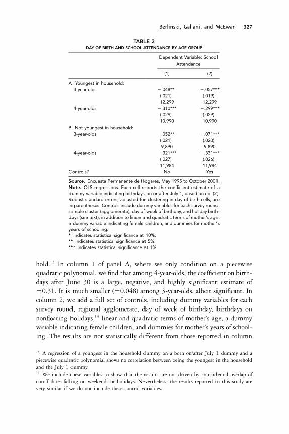
TABLE 6DAY OF BIRTH AND MATERNAL LABOR OUTCOMES BY AGE GROUP

Dependent Variable

Mother WorksMother Works

Full Time Hours Worked

(1) (2) (3) (4) (5) (6)


3-year-olds .005 .009 �.007 �.005 �.124 �.082(.032) (.029) (.029) (.026) (1.242) (1.174)12,299 12,299 12,221 12,221 12,221 12,221

4-year-olds �.066** �.038 �.085** �.058* �3.339** �2.354*(.033) (.031) (.033) (.031) (1.396) (1.350)10,990 10,990 10,911 10,911 10,911 10,911


3-year-olds �.012 �.011 .009 .009 .468 .437(.029) (.031) (.029) (.030) (1.213) (1.260)9,890 9,890 9,843 9,843 9,843 9,843

4-year-olds �.002 .003 �.012 �.007 �.771 �.553(.027) (.026) (.025) (.023) (1.059) (1.026)11,984 11,984 11,930 11,930 11,930 11,930

Controls? No Yes No Yes No Yes

Source. Encuesta Permanente de Hogares, May 1995 to October 2001.Note. OLS regressions. Each cell reports the coefficient estimate of a dummy variable indicating birth-days on or after July 1 (based on eq. [3]). Robust standard errors, adjusted for clustering in day-of-birthcells, are in parentheses. Controls include dummy variables for each survey round, sample cluster (ag-glomerate), day of week of birthday, and holiday birthdays, in addition to linear and quadratic terms ofmother’s age, a dummy variable indicating female children, and dummies for mother’s years of schooling.* Indicates statistical significance at 10%.** Indicates statistical significance at 5%.*** Indicates statistical significance at 1%.

servables is plausible, our results might still be biased, although the directionof the bias is not clear.

C. School Attendance and Maternal Labor OutcomesIn table 6, we report estimates from reduced-form regressions of mother’slabor market outcomes on a dummy variable indicating births on or after July1. The dependent variables include whether mothers were employed last week,whether mothers worked for at least 20 hours last week (full time), and thenumber of hours worked last week. We estimate separate OLS regressions ofequation (3) for children aged 3 and 4. All regressions include as a controlfunction a piecewise quadratic of birth date, while regressions in even columnsinclude a full set of controls. Because children born on or after July 1 are lesslikely to attend school, we expect a negative effect for maternal labor outcomesof being born on or after July 1.

In the samples of 3-year-olds, none of the coefficients are statistically dis-tinguishable from zero. This is perhaps not surprising given the relatively


Figure 4. Maternal labor outcomes and child’s day of birth, by age group. Dots indicate means ofdummy variables indicating employment (left), full-time employment (middle), and weekly hours of work(right). Solid lines show fitted values of piecewise quadratic polynomials. Source: Encuesta Permanentede Hogares, 1995–2001.

small difference in school attendance around the July 1 cutoff for such children.For children aged 4 who are the youngest in the household, the coefficientsin table 6 range between �0.066 and �0.038 when a dichotomous indicatorof mother’s employment is the dependent variable. Coefficients range between�0.085 and �0.058 when the dependent variable is work for more than 20hours a week. In columns 5 and 6, mothers of children born in the secondsemester of the year work between 2.4 and 3.4 fewer hours in the previousweek. Not surprisingly, given the evidence from the previous section, thecoefficients from fully specified models are less negative. The pattern of thereduced-form results just described is corroborated in figure 4, which presentsunsmoothed means and fitted values for children aged 4, both for the youngestchildren (upper panels) and not youngest (lower panels).

Despite the fact that there is a significant increase in preschool attendanceamong children aged 4 who are not the youngest in the household, there isno evidence of changes in employment or hours of work for their mothers.In theory, it is plausible that there could be an effect on these outcomes forthe mothers of these children as the child care provided by preschool attendanceof at least one of their children contributes toward reducing the total cost ofchild care. However, the result implies that this contribution is small relative


TABLE 7PRESCHOOL ATTENDANCE AND MATERNAL LABOR OUTCOMES, 4 YEAR-OLDS:

TWO-STAGE LEAST SQUARES ESTIMATES

Dependent Variable

Mother WorksMother Works

Full Time Hours Worked

(1) (2) (3) (4) (5) (6)


4-year-olds .213* .127 .270** .191* 10.642** 7.779*(.110) (.106) (.111) (.104) (4.595) (4.556)10,990 10,990 10,911 10,911 10,911 10,911


4-year-olds .006 �.008 .037 .021 2.420 1.670(.084) (.078) (.079) (.070) (3.347) (3.114)11,984 11,984 11,930 11,930 11,930 11,930

Controls? No Yes No Yes No Yes

Source. Encuesta Permanente de Hogares, May 1995 to October 2001.Note. Each cell reports the coefficient estimate of a dummy variable indicating school attendance froma TSLS regression, based on eq. (1) and including a piecewise quadratic polynomial of birthdate. Theexcluded instrument is Z. Robust standard errors, adjusted for clustering in day-of-birth cells, are inparentheses. The sample size of each regression is reported below coefficients and standard errors.Controls include dummy variables for each survey round, sample cluster (agglomerate), day of week ofbirthday, and holiday birthdays, in addition to linear and quadratic terms of mother’s age, a dummyvariable indicating female children, and dummies for mother’s years of schooling.* Indicates statistical significance at 10%.** Indicates statistical significance at 5%.*** Indicates statistical significance at 1%.

to the cost of child care for the other children and does not affect the decisionof the mother to either work or work for more hours.

Table 7 reports two-stages least squares estimates, which are simply thereduced-form estimates from table 6 divided by the changes in the probabilityof attendance estimated among 4-year-olds in table 3. Among the subsampleof youngest children (panel A), the model with the full set of controls suggeststhat mothers who are induced to enroll their children in kindergarten are 12.7percentage points more likely to work, although the estimate is not precise.Furthermore, mothers are 19.1 percentage points more likely to work morethan 20 hours per week, and they work, on average, 7.8 more hours per weekas a consequence of their youngest child attending preschool. Both estimatesare statistically significant at the 10% level. The point estimates of the binaryemployment measures are consistent with the upper end of estimates reportedin Berlinski and Galiani (2007), who used a different EPH sample and anempirical strategy that exploits temporal and regional variation in preschoolconstruction.

In table 8, we report a set of robustness checks for the two-stages least


TABLE 8PRESCHOOL ATTENDANCE AND MATERNAL LABOR OUTCOMES, 4-YEAR-OLDS: TWO-STAGE LEAST SQUARES

ESTIMATES, ALTERNATIVE SPECIFICATIONS, AND SAMPLES

(1) (2) (3) (4) (5) (6)

A. 4 Years Old, Youngest in Household

Mother works .127 .050 .086 .019 .197 .056(.106) (.137) (.202) (.153) (.131) (.187)

10,990 10,990 10,990 5,454 10,587 10,990Mother works full time .191* .076 .181 .075 .245* .208

(.104) (.137) (.206) (.157) (.125) (.155)10,911 10,911 10,911 5,416 10,511 10,911

Hours worked 7.779* 5.122 8.642 4.190 10.217* 13.741**(4.556) (6.101) (9.177) (6.870) (5.496) (6.731)10,911 10,911 10,911 5,416 10,511 10,911

B. 4 Years Old, Not Youngest in Household

Mother works �.008 .067 .142 .091 �.030 .294*(.078) (.097) (.128) (.114) (.095) (.173)

11,984 11,984 11,984 5,906 11,515 11,984Mother works full time .021 .006 .105 .056 .014 .110

(.070) (.085) (.111) (.096) (.087) (.143)11,930 11,930 11,930 5,879 11,465 11,930

Hours worked 1.670 .627 5.492 3.148 .867 11.526(3.114) (3.979) (5.404) (4.552) (3.716) (7.819)11,930 11,930 11,930 5,879 11,465 11,930

Piecewise polynomial Quadratic Cubic Quartic Quadratic Quadratic QuadraticSample Full Full Full Born

April–SeptemberBorn 7/1–7

and 6/24–30excluded

Full withsurvey

weights

Source. Encuesta Permanente de Hogares, May 1995 to October 2001.Note. The “Full” sample and estimates from col. 1 are based on even columns in table 7. Each cellreports the coefficient estimate of a dummy variable indicating school attendance from a TSLS regression,following the specification in table 7. Robust standard errors, adjusted for clustering in day-of-birth cells,are in parentheses. All regressions include dummy variables for each survey round, sample cluster (ag-glomerate), day of week of birthday, and holiday birthdays, in addition to linear and quadratic terms ofmother’s age, a dummy variable indicating female children, and dummies for mother’s years of schooling.* Indicates statistical significance at 10%.** Indicates statistical significance at 5%.*** Indicates statistical significance at 1%.

squares estimates.18 Column 1 is the benchmark, reproducing estimates fromcolumns 2, 4, and 6 in table 7. In columns 2 and 3, we use cubic and quarticpolynomials, respectively. In the remaining columns of table 5, we use apiecewise quadratic polynomial but within different samples. In column 4,

18 We have also estimated the effect of preschool attendance on maternal labor outcomes usinglocally weighted regressions (results available upon request from the authors). The estimates forthe youngest in the household are similar in magnitude to those presented in table 7 and robustto the choice of bandwidth. However, they are imprecisely estimated. For children who are notthe youngest in the household the magnitudes of the estimates tend to be positive but are quitesensitive to the bandwidth choice and are also imprecisely estimated.


we focus on the sample of children born between April and September. Incolumn 5, we drop a 1-week window on each side of the cutoff. In column6, we use survey weights.19 The results in panel A are similarly signed butless precise than in the benchmark specification. The most noticeable differenceis that when we weight observations using the survey weights, the results forthe nonyoungest children in the household (panel B) tend to be similar tothe results for the youngest children.

D. Heterogeneous Effects

We have shown that the effect of the enrollment rule on preschool attendanceis not affected by whether there are younger siblings in the household. How-ever, the maternal labor market response to the preschool enrollment rule for4-year-old children is remarkably different for the mothers of children withand without younger siblings. We next explore whether other variables thatare likely to affect maternal home and market productivity, such as age andschooling, affect their behavioral responses to the enrollment rule.

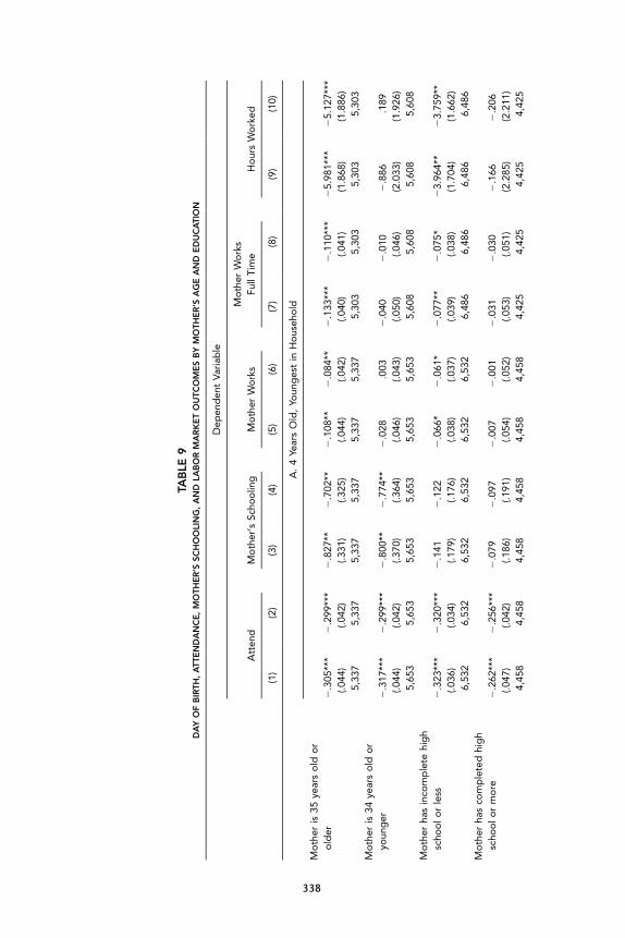
In table 9, we report estimates from OLS regressions of school attendance,mother’s schooling, mother’s employment, employment for more than 20 hourslast week, and hours worked last week on a dummy variable indicating birthson or after July 1 for four samples of 4-year-old children: mothers aged 35or older, mothers younger than 35 years of age, mothers with incomplete highschool or lower educational achievement, and mothers with complete highschool education or higher educational achievement. All regressions controlfor a piecewise quadratic of birth date, while regressions in even columnsinclude a full set of controls. Panel A presents results for children who arethe youngest in the household and panel B for other children.

We find that the effect of the enrollment rule on preschool attendance isnot significantly different between children with mothers of different ages.There is some evidence that the preschool attendance of youngest children inthe household with mothers who have lower education is more sensitive tothe enrollment rule—about 6 percentage points—but this difference is notstatistically significant. The lack of balancing on maternal education persistsfor the youngest children in the household regardless of their mothers’ agegroup.20 Dividing the sample by maternal education seemingly resolves thelack of balancing in maternal education around the cutoff. However, caution

19 Because in the placebo experiments from table 5 the effect on attendance is close to zero, thecorresponding two-stage least squares estimates are close to zero as well.20 In particular, this also suggests that this unbalance is not the result of the younger mothersdropping out of school because they cannot enroll their children at school.


is needed since this might just be a mechanical consequence of censoring thedependent variable.

In terms of labor market responses, the effects are still concentrated amongmothers for whom the child is the youngest in the household. Despite thefact that the enrollment rule produces similar responses in terms of preschoolattendance for the different groups, we find that the effects on employmentand hours of work are driven by older and less educated mothers. For example,among the subsample of youngest children (panel A), the model with the fullset of controls suggests that mothers with children born on or after July 1were 8.4 percentage points less likely to work, 11 percentage points less likelyto work full time, and worked 5 hours less per week. This is equivalent toan effect of preschool attendance on employment of 19 percentage points, onfull-time work of 23 percentage points, and on hours worked of 11.65 hours.21

We speculate that older mothers with young children are either less likely tohave additional children or have more attachment to the labor market andthus are more responsive when their youngest child starts preschool. In theabsence of a comprehensive welfare system, as in Argentina, less-educatedmothers may also have the need to return to work as soon as it is feasible.

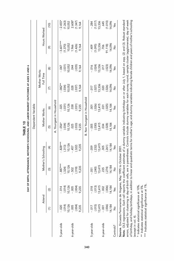
E. Day of Birth and Maternal Outcomes for Primary School ChildrenIn table 10, we reproduce estimates for school attendance, mother’s schooling,mother’s employment, employment for more than 20 hours last week, andhours worked last week for children aged 5 and 6 on July 1 of the surveyyear. School enrollment is uniformly high at these ages, and there is noenrollment effect of July 1 births. The correlation between maternal schoolingand being born in the second semester still persists. We find that for childrenaged 5 who are the youngest in the household the maternal labor outcomescoefficients in table 10 tend to be of similar sign and magnitude to those ofthe youngest children aged 4 we reported in table 6. We find no systematiceffects for children aged 6 or for those children who are not the youngest inthe household.

Why do we observe employment effects for children aged 5 when there isno school attendance discontinuity? One explanation is that the result is astatistical artifact reflecting a lack of balancing in the observables. Althoughthis is theoretically plausible, it does not explain why, in our sample, such acorrelation does not exist at age 6. An alternative explanation is that althoughsome mothers find employment at the moment when their children startkindergarten, for others it takes time to find suitable employment so that

21 Two-stage least squares results are available from the authors upon request.

338

TAB

LE9

DA

YO

FB

IRTH

,A

TTE

ND

AN

CE

,M

OTH

ER

’SSC

HO

OLI

NG

,A

ND

LAB

OR

MA

RK

ET

OU

TCO

ME

SB

YM

OTH

ER

’SA

GE

AN

DE

DU

CA

TIO

N

Dep

end

ent

Vari

able

Att

end

Mo

ther

’sSc

hoo

ling

Mo

ther

Wo

rks

Mo

ther

Wo

rks

Full

Tim

eH

our

sW

ork

ed

(1)

(2)

(3)

(4)

(5)

(6)

(7)

(8)

(9)

(10)

A.

4Ye

ars

Old

,Yo

ung

est

inH

ous

eho

ld

Mo

ther

is35

year

so

ldo

ro

lder

�.3

05**

*�

.299

***

�.8

27**

�.7

02**

�.1

08**

�.0

84**

�.1

33**

*�

.110

***

�5.

981*

**�

5.12

7***

(.044

)(.0

42)

(.331

)(.3

25)

(.044

)(.0

42)

(.040

)(.0

41)

(1.8

68)

(1.8

86)

5,33

75,

337

5,33

75,

337

5,33

75,

337

5,30

35,

303

5,30

35,

303

Mo

ther

is34

year

so

ldo

ryo

ung

er�

.317

***

�.2

99**

*�

.800

**�

.774

**�

.028

.003

�.0

40�

.010

�.8

86.1

89(.0

44)

(.042

)(.3

70)

(.364

)(.0

46)

(.043

)(.0

50)

(.046

)(2

.033

)(1

.926

)5,

653

5,65

35,

653

5,65

35,

653

5,65

35,

608

5,60

85,

608

5,60

8M

oth

erha

sin

com

ple

tehi

gh

scho

ol

or

less

�.3

23**

*�

.320

***

�.1

41�

.122

�.0

66*

�.0

61*

�.0

77**

�.0

75*

�3.

964*

*�

3.75

9**

(.036

)(.0

34)

(.179

)(.1

76)

(.038

)(.0

37)

(.039

)(.0

38)

(1.7

04)

(1.6

62)

6,53

26,

532

6,53

26,

532

6,53

26,

532

6,48

66,

486

6,48

66,

486

Mo

ther

has

com

ple

ted

hig

hsc

hoo

lo

rm

ore

�.2

62**

*�

.256

***

�.0

79�

.097

�.0

07�

.001

�.0

31�

.030

�.1

66�

.206

(.047

)(.0

42)

(.186

)(.1

91)

(.054

)(.0

52)

(.053

)(.0

51)

(2.2

85)

(2.2

11)

4,45

84,

458

4,45

84,

458

4,45

84,

458

4,42

54,

425

4,42

54,

425

339

B.

4Ye

ars

Old

,N

ot

Youn

ges

tin

Ho

useh

old

Mo

ther

is35

or

old

er�

.338

***

�.3

45**

*�

.023

�.1

63.0

17.0

31�

.019

�.0

11�

.686

�.0

50(.0

51)

(.041

)(.5

68)

(.553

)(.0

65)

(.059

)(.0

59)

(.052

)(2

.430

)(2

.212

)2,

909

2,90

92,

909

2,90

92,

909

2,90

92,

897

2,89

72,

897

2,89

7M

oth

eris

youn

ger

than

35�

.315

***

�.3

25**

*.0

09�

.051

�.0

06�

.008

�.0

07�

.006

�.6

74�

.661

(.033

)(.0

32)

(.262

)(.2

60)

(.029

)(.0

27)

(.026

)(.0

23)

(1.0

96)

(1.0

59)

9,07

59,

075

9,07

59,

075

9,07

59,

075

9,03

39,

033

9,03

39,

033

Mo

ther

has

inco

mp

lete

hig

hsc

hoo

lo

rle

ss�

.308

***

�.3

25**

*.1

04.0

53.0

01�

.001

�.0

22�

.026

�.8

57�

.940

(.034

)(.0

31)

(.167

)(.1

63)

(.028

)(.0

28)

(.026

)(.0

24)

(1.1

91)

(1.1

40)

8,27

18,

271

8,27

18,

271

8,27

18,

271

8,23

68,

236

8,23

68,

236

Mo

ther

has

com

ple

ted

hig

hsc

hoo

lo

rm

ore

�.3

36**

*�

.326

***

.190

.109

.007

.014

.027

.037

�.0

08.6

00(.0

42)

(.040

)(.2

07)

(.200

)(.0

52)

(.048

)(.0

49)

(.046

)(2

.043

)(1

.997

)3,

713

3,71

33,

713

3,71

33,

713

3,71

33,

694

3,69

43,

694

3,69

4C

ont

rols

?N

oYe

sN

oYe

sN

oYe

sN

oYe

sN

oYe

s

Sour

ce.

Enc

uest

aP

erm

anen

ted

eH

og

ares

,M

ay19

95to

Oct

ob

er20

01.

No

te.

OLS

reg

ress

ions

.E

ach

cell

rep

ort

sth

eco

effic

ient

esti

mat

eo

fa

dum

my

vari

able

ind

icat

ing

bir

thd

ays

on

or

afte

rJu

ly1,

bas

edo

neq

q.

(2)

and

(3).

Ro

bus

tst

and

ard

erro

rs,

adju

sted

for

clus

teri

ngin

day

-of-

bir

thce

lls,

are

inp

aren

thes

es.

Co

ntro

lsin

clud

ed

umm

yva

riab

les

for

each

surv

eyro

und

,sa

mp

lecl

uste

r(a

gg

lom

erat

e),d

ayo

fw

eek

of

bir

thd

ay,a

ndho

liday

bir

thd

ays,

inad

dit

ion

tolin

ear

and

qua

dra

tic

term

sfo

rm

oth

er’s

age;

and

dum

my

vari

able

sin

dic

atin

gfe

mal

ech

ildre

nan

dye

ars

ofm

oth

er’s

scho

olin

g(e

xcep

tin

col.

4).

*In

dic

ates

stat

isti

cals

igni

fican

ceat

10%

.**

Ind

icat

esst

atis

tica

lsig

nific

ance

at5%

.**

*In

dic

ates

stat

isti

cals

igni

fican

ceat

1%.

340

TAB

LE1

0D

AY

OF

BIR

TH,

ATT

EN

DA

NC

E,

MO

THE

R’S

SCH

OO

LIN

G,

AN

DLA

BO

RM

AR

KE

TO

UTC

OM

ES

AT

AG

ES

5A

ND

6

Dep

end

ent

Vari

able

Att

end

Mo

ther

’sSc

hoo

ling

Mo

ther

Wo

rks

Mo

ther

Wo

rks

Full

Tim

eH

our

sW

ork

ed

(1)

(2)

(3)

(4)

(5)

(6)

(7)

(8)

(9)

(10)

A.

Youn

ges

tin

Ho

useh

old

5-ye

ar-o

lds

�.0

20�

.014

�.8

87**

*�

.828

***

�.0

56*

�.0

25�

.082

**�

.047

�3.

601*

**�

2.45

5*(.0

14)

(.014

)(.3

24)

(.313

)(.0

34)

(.031

)(.0

34)

(.031

)(1

.370

)(1

.263

)10

,126

10,1

2610

,126

10,1

2610

,126

10,1

2610

,052

10,0

5210

,052

10,0

526-

year

-old

s�

.005

�.0

05�

.502

�.4

57.0

25.0

38.0

28.0

441.

966

2.60

8*(.0

04)

(.004

)(.3

18)

(.322

)(.0

33)

(.031

)(.0

37)

(.035

)(1

.426

)(1

.347

)9,

235

9,23

59,

235

9,23

59,

235

9,23

59,

164

9,16

49,

164

9,16

4

B.

No

tYo

ung

est

inH

ous

eho

ld

5-ye

ar-o

lds

�.0

17�

.018

�.0

51�

.059

�.0

05.0

01�

.017

�.0

16�

.409

�.2

84(.0

15)

(.013

)(.2

40)

(.232

)(.0

30)

(.026

)(.0

27)

(.024

)(1

.095

)(1

.017

)13

,415

13,4

1513

,415

13,4

1513

,415

13,4

1513

,336

13,3

3613

,336

13,3

366-

year

-old

s�

.001

�.0

02.2

35.3

05.0

34.0

31.0

20.0

17.7

06.6

45(.0

06)

(.006

)(.2

74)

(.261

)(.0

28)

(.025

)(.0

26)

(.023

)91

.118

)(1

.010

)14

,184

14,1

8414

,184

14,1

8414

,184

14,1

8414

,096

14,0

9614

,096

14,0

96C

ont

rols

?N

oYe

sN

oYe

sN

oYe

sN

oYe

sN

oYe

s

Sour

ce.

Enc

uest

aP

erm

anen

ted

eH

og

ares

,M

ay19

95to

Oct

ob

er20

01.

No

te.

OLS

reg

ress

ions

.E

ach

cell

rep

ort

sth

eco

effic

ient

esti

mat

eo

fa

dum

my

vari

able

ind

icat

ing

bir

thd

ays

on

or

afte

rJu

ly1,

bas

edo

neq

q.

(2)

and

(3).

Ro

bus

tst

and

ard

erro

rs,

adju

sted

for

clus

teri

ngin

day

-of-

bir

thce

lls,

are

inp

aren

thes

es.

Co

ntro

lsin

clud

ed

umm

yva

riab

les

for

each

surv

eyro

und

,sa

mp

lecl

uste

r(a

gg

lom

erat

e),d

ayo

fw

eek

of

bir

thd

ay,a

ndho

liday

bir

thd

ays,

inad

dit

ion

tolin

ear

and

qua

dra

tic

term

sfo

rm

oth

er’s

age;

and

dum

my

vari

able

sin

dic

atin

gfe

mal

ech

ildre

nan

dye

ars

ofm

oth

er’s

scho

olin

g(e

xcep

tin

col.

4).

*In

dic

ates

stat

isti

cals

igni

fican

ceat

10%

.**

Ind

icat

esst

atis

tica

lsig

nific

ance

at5%

.**

*In

dic

ates

stat

isti

cals

igni

fican

ceat

1%.


some effects appear at age 5. Given the similarity in the magnitude of thecoefficients between ages 4 and 5, one suspects that this cannot be the wholestory. A complementary explanation is that, at age 5, the dummy for beingborn on or after July 1 picks up the difference between being enrolled inkindergarten and primary school. If the maturity of a child plays a role onthe decision of a mother to go work, the transition from kindergarten toprimary school may be interpreted by families as a signal that in-home careis no longer necessary.22 This is consistent with the fact that no such effectappears at age 6.

V. ConclusionExpanding preschool education has the dual goals of improving child outcomesand work incentives for mothers. This study provides evidence on the second,identifying the impact of preschool attendance on maternal labor marketoutcomes in Argentina. A major challenge in identifying the causal effect ofpreschool attendance on parental outcomes is nonrandom selection into earlyeducation. We address this by relying on plausibly exogenous variation inpreschool attendance that is induced when children are born on either side ofArgentina’s enrollment cutoff date of July 1. Because of enrollment cutoffdates, 4-year-olds born just before July 1 are 0.3 more likely to attend pre-school. Our regression-discontinuity estimates compare maternal employmentoutcomes of 4-year-old children on either side of this cutoff, identifying effectsamong the subset of complying households (who are perhaps more likely toface constraints on their level 2 preschool attendance).

Our findings suggest that, on average, 13 mothers start to work for every100 youngest children in the household who start preschool (although, in ourpreferred specification, this estimate is not statistically significant at conven-tional levels). Furthermore, mothers are 19.1 percentage points more likelyto work for more than 20 hours a week (i.e., more time than their childrenspend in school) and they work, on average, 7.8 more hours per week as aconsequence of their youngest offspring attending preschool. We find no effecton maternal labor outcomes when a child who is not the youngest in thehousehold attends preschool. Finally, we find that at the point of transitionfrom kindergarten to primary school some employment effects persist.

Our preferred estimates condition on mother’s schooling and other exog-enous covariates, given evidence that mother’s schooling is unbalanced in the

22 A more practical explanation is that primary schools may have longer school days and henceprovide a larger implicit subsidy. Nevertheless, primary schools, like preschools, also operate mainlyon a two-shift schedule.


vicinity of the July 1 cutoff in the sample of 4-year-olds. Using a large sampleof natality records, we found no evidence that this is due to precise birth datemanipulation by parents. Other explanations, like sample selection, are alsonot fully consistent with the data, and we must remain agnostic on this point.Despite this shortcoming, the credibility of the estimates is partly enhancedby the consistency of point estimates with Argentine research using a differentEPH sample and sources of variation in preschool attendance (Berlinski andGaliani 2007).

A growing body of research suggests that preprimary school can improveeducational outcomes for children in the short and long run (Blau and Currie2006; Schady 2006). This study provides further evidence that, all else equal,an expansion in preschool education may enhance the employment prospectsof mothers of children in preschool age.23

ReferencesAnderson, Patricia M., and Philip B. Levine. 2000. “Child Care and Mothers’ Em-

ployment Decisions.” In Finding Jobs: Work and Welfare Reform, ed. David Cardand Rebecca M. Blank. New York: Russell Sage Foundation.

Baker, Michael, Jonathan Gruber, and Kevin Milligan. 2008. “Universal Childcare,Maternal Labor Supply and Family Well-Being.” Journal of Political Economy 116:709–45.

Barua, Rashmi. 2007. “Intertemporal Substitution in Maternal Labor Supply: Evi-dence Using State School Entrance Age Laws.” Unpublished manuscript, BostonUniversity.

Belizan, Jose M., Fernando Althabe, Fernando C. Barros, and Sophie Alexander.1999. “Rates and Implications of Caesarean Sections in Latin America: EcologicalStudy.” British Medical Journal 319:1397–1400.

Berlinski, Samuel, and Sebastian Galiani. 2007. “The Effect of a Large Expansionof Pre-Primary School Facilities on Preschool Attendance and Maternal Employ-ment.” Labour Economics 14:665–80.

Berlinski, Samuel, Sebastian Galiani, and Paul Gertler. 2009. “The Effect of Pre-Primary Education on Primary School Performance.” Journal of Public Economics93:219–34.

Berlinski, Samuel, Sebastian Galiani, and Marco Manacorda. 2008. “Giving Childrena Better Start: Preschool Attendance and School-Age Profiles.” Journal of PublicEconomics 92:1416–40.

Blau, David, and Janet Currie. 2006. “Pre-School, Day Care, and After School Care:Who’s Minding the Kids?” In Handbook of the Economics of Education, vol. 2, ed.Eric Hanushek and Finis Welch. Amsterdam: Elsevier.

Bound, John, and David A. Jaeger. 2000. “Do Compulsory Attendance Laws Alone

23 However, as a referee notes, the large-scale expansion of preschool might have additional effectsnot reflected in our empirical results. For example, one could imagine that it increases fertility,which could have countervailing effects on labor supply among women.


Explain the Association between Earnings and Quarter of Birth?” In Research inLabor Economics: Worker Well-Being, ed. Solomon W. Polacheck. New York: JAI.

Bound, John, David A. Jaeger, and Regina M. Baker. 1995. “Problems with In-strumental Variables Estimation When the Correlation between the Instrumentsand the Endogenous Explanatory Variable Is Weak.” Journal of the American Sta-tistical Association 90:443–50.

Browning, Martin. 1992. “Children and Household Economic Behavior.” Journal ofEconomic Literature 30:1434–75.

Cascio, Elizabeth U. 2009. “Maternal Labor Supply and the Introduction of Kin-dergartens into American Public Schools.” Journal of Human Resources 44:140–70.

Dickert-Conlin, Stacy, and Amitabh Chandra. 1999. “Taxes and the Timing ofBirths.” Journal of Political Economy 107:161–77.

Fitzpatrick, Maria D. 2008. “Preschoolers Enrolled and Mothers at Work? The Effectsof Universal Pre-Kindergarten.” Unpublished manuscript, Stanford University.

Galiani, Sebastian, Daniel Heymann, and Mariano Tommasi. 2003. “Great Expec-tations and Hard Times: The Argentina Convertibility Plan.” Economıa 4:109–60.

Galiani, Sebastian, and Stephen Nickell. 1999. “Unemployment in Argentina in the1990s.” Working Paper DTE 219, Instituto Torcuato Di Tella, Buenos Aires.

Gans, Joshua S., and Andrew Leigh. 2009. “Born on the First of July: An (Un)naturalExperiment in Birth Timing.” Journal of Public Economics 93:246–63.

Gelbach, Jonah B. 2002. “Public Schooling for Young Children and Maternal LaborSupply.” American Economic Review 92:307–22.

Hahn, Jinyong, Petra Todd, and Wilbert van der Klaauw. 2001. “Identification andEstimation of Treatment Effects with a Regression-Discontinuity Design.” Econ-ometrica 69:201–9.

Imbens, Guido W., and Joshua D. Angrist. 1994. “Identification and Estimation ofLocal Average Treatment Effects.” Econometrica 62:467–75.

Imbens, Guido W., and Thomas Lemieux. 2008. “Regression Discontinuity Designs:A Guide to Practice.” Journal of Econometrics 142:615–35.

Lee, David S. 2008. “Randomized Experiments from Non-Random Selection in U.S.House Elections.” Journal of Econometrics 142:675–97.

Lee, David S., and David Card. 2008. “Regression Discontinuity Inference withSpecification Error.” Journal of Econometrics 142:655–74.

McCrary, Justin, and Heather Royer. 2006. “The Effect of Maternal Education onFertility and Infant Health: Evidence from School Entry Laws Using Exact Dateof Birth.” Unpublished manuscript, University of Michigan and Case WesternReserve University.

McEwan, Patrick J., and Joseph S. Shapiro. 2008. “The Benefits of Delayed PrimarySchool Enrollment: Discontinuity Estimates Using Exact Birth Dates.” Journal ofHuman Resources 43:1–29.

Mussa, Michael. 2002. Argentina and the Fund: From Triumph to Tragedy. Washington,DC: Petersen Institute.

Myers, Robert J. 1995. “Preschool Education in Latin America: Estate [sic] of Prac-tice.” Working Paper no. 1, Partnership for Educational Revitalization (PREAL),Washington, DC.

OECD (Organization for Economic Cooperation and Development). 2002. “Strength-


ening Early Childhood Programs: A Policy Framework.” In Education Policy Anal-ysis. Paris: OECD.

Schady, Norbert. 2006. “Early Childhood Development in Latin America and theCaribbean.” Economıa 6:185–225.

Schlosser, Analıa. 2006. “Public Preschool and the Labor Supply of Arab Mothers:Evidence from a Natural Experiment.” Unpublished manuscript, Hebrew Uni-versity of Jerusalem.

van der Klaauw, Wilbert. 2002. “Estimating the Effect of Financial Aid Offers onCollege Enrollment: A Regression-Discontinuity Approach.” International EconomicReview 43:1249–87.

preschool and maternal labor market outcomes:...

Documents