prepublicaciones del departamento de … influence of... · the large solutions of quasilinear...
TRANSCRIPT

PREPUBLICACIONES DEL DEPARTAMENTODE MATEMÁTICA APLICADA
UNIVERSIDAD COMPLUTENSE DE MADRIDMA-UCM 2012-10
The influence of sources terms on the boundary behavior of the large solutions of quasilinear elliptic equations.
The power like case
S.Alarcón, G.Díaz and J.M.Rey.
Septiembre-2012
http://www.mat.ucm.es/deptos/mae-mail:matemá[email protected]


The influence of sources terms on the boundary behavior ofthe large solutions of quasilinear elliptic equations. The power
like caseTo appear in Zeitschrift fuer Angewandte Mathematik und Physik (ZAMP)
S. Alarcon, G. Dıaz and J. M. Rey ∗
Abstract
We study the explosive expansion near the boundary of the large solutions of the equation
−∆pu+ um = f in Ω
where Ω is an open bounded set of RN, N > 1, with adequately smooth boundary, m > p− 1 > 0 and fis a continuous nonnegative function in Ω. Roughly speaking, we show that the number of explosive termsin the asymptotic boundary expansion of the solution is finite, but it goes to infinity as m goes to p−1. Forillustrative choices of the sources, we prove that the expansion consists of two possible geometrical andnon–geometrical parts. For low explosive sources the non–geometrical part does not exist, all coefficientsdepend on the diffusion and the geometry of the domain. For high explosive sources there are coefficients,relative to the non–geometrical part, independent on Ω and the diffusion. In this case, the geometricalpart can not exist and we say then that the source is very high explosive. We emphasize that low orhigh explosive sources can cause different geometrical properties in the expansion for a given interiorstructure of the differential operator. This paper is strongly motivated by the applications, in particular bythe non-Newtonian fluid theory where p = 2 involves rheological properties of the medium.
1 IntroductionThis paper deals with the asymptotic behavior of solutions of the equation
− div(|∇u|p−2∇u) + um = f in Ω (1)
where Ω is a bounded domain in RN, N > 1, f ∈ C(Ω), m > 0 and p > 1. As it is usual, we denote by−∆p the leading part of the differential operator. More precisely, our interest is focussed on the solutionswith an explosive behavior at the boundary
u(x) → ∞ as x → ∂Ω, (2)
usually called large (explosive, boundary blow-up) solutions. A strong motivation of the paper is based onthe applications where the values p = 2 have a capital role (see below).
As it is well known for the homogeneous case, f ≡ 0, the large solutions have been studied for severalauthors provided the extended Keller–Osserman condition
m > p− 1 (3)
∗S.A. was partially supported by Fondecyt Grant No. 11110482, USM Grant No. 121210 and Programa Basal, CMM, U. de Chile.G.D. is supported by the projects MTM 2008-06208 of DGISGPI (Spain) and the Research Group MOMAT (Ref. 910480) fromBanco Santander and UCM. The work of J.M.R. has been done in the framework of project MTM2011-22658 of the Spanish Ministryof Science and Innovation and the Research Group MOMAT (Ref. 910480) supported by Banco Santander and UCM.
KEYWORDS: Large solutions, asymptotic behavior, sub and supersolutions.AMS SUBJECT CLASSIFICATIONS: 35B40,35J25, 35J65.
1

2 S. Alarcon, G. Dıaz and J.M. Rey
(see, for instance, [11] or [21]). An extensive amount of references, mainly for the uniformly elliptic casep = 2, is collected in monograph [22] (see also [5] and [6]). Our main comments, in this paper, dealpreferably with the general case governed by the nonlinear leading part corresponding to p = 2, stronglymotivated by the applications. From the mathematical point of view, the main difference with the linear caseis that the differential operator is not uniformly elliptic: degenerate for p > 2 and singular for 1 < p < 2.From the applications point of view, a main difficulty appears: we must know the precise dependence on pin the boundary behavior of solutions which cannot be deduced from the case p = 2 by a simple way. Afirst study of problem (1)–(2) was made in [11] where existence, uniqueness and blow up rate of solutionsfor certain functions f ≥ 0 were proved, under assumption (3) (see also [18, 21], where the previous resultswere extended to more general nonlinearities in case f ≡ 0). We note that these well known results showthat the first term of the expansion near the boundary of large solutions is uniform and independent on thegeometry of ∂Ω (see again [11] and [21] as well as [13] and the references therein). To the best of ourknowledge, we do not know any work on the study the influence of the geometry of the domain on largesolutions of (1) when f ≡ 0. Then, an interesting question is to know how non–homogeneous sources andthe geometry of the domain can influence in the asymptotic expansion near the boundary of solutions of(1)–(2).
We recall that for p = 2 and f ≡ 0 the dependence on the geometry is known from the pioneer work [8]or from [1, 3, 4, 5, 6, 7, 17], for instance. In these works one proves that the geometrical influence appearsfrom the second order term of the explosive expansion. Our extensions are nontrivial due to the nonlinearnature of the operator with p = 2. Moreover, as in [1], the influence of non–null sources provides a moredeep knowledge of the nature of the explosiveness properties of the solutions. We note that large solutionsunder non–null sources have been also studied in [20], [23] or [24] with different purposes.
As it is usual, the properties near the boundary employ the distance function dist(x, ∂Ω), here denotedby d(x). As it is well known, if the boundary is bounded with ∂Ω ∈ Ck, k ≥ 1, it follows from [15] theexistence of a positive constant δ0, depending only on ∂Ω, such that d(·) ∈ Ck in the parallel strip near theboundary
Ωδ0 = x ∈ Ω : d(x) < δ0. (4)
Moreover, from the results of [15], also can be deduced the important properties for x ∈ Ωδ0 as
|∇d(x)| ≡ 1 and ∆d(x) = −(N− 1)H(x(x)) + o(1),
where x(x) is a point on ∂Ω such that |x − x(x)| = d(x) and H(x(x)) denotes the mean curvature of ∂Ωat x(x). The simplest geometry occurs on balls, as Ω = BR(0), for which
∆d(x) = −N− 1
|x|, |x| < R.
These geometrical properties of the domain can to take part in the asymptotic expansion near the boundary.Indeed this influence occurs on secondary terms under more regularity assumptions on the boundary. Itis obtained by considering terms containing the mean curvature neglected in the leading coefficient of theexpansion.
We emphasize that the existence of large solutions of (1), for f ≡ 0, is based on the Keller–Ossermancondition. This inequality is also a necessary assumption in the non–homogeneous case f ≡ 0. In order tosimplify, the main goal of this paper is to study the influence of sources with the property
f(x) ≈ f0(d(x)
)−ατm as d(x) → 0, f ≥ 0,
whereατ =
p+ τ
m− p+ 1(τ is a non–negative integer) (5)
(we note that, by construction, f0 ≥ 0). As we comment below, we say that the source causes a lowexplosion if τ = 0, and the source causes a high explosion if τ > 0 and f0 > 0. More precisely, in thispaper we consider continuous and nonnegative sources satisfying
f(x) =(d(x)
)−ατm(f0 +
Mτ∑n=1
fn(d(x)
)n), x ∈ Ωδ0 , (6)

The influence of sources terms on the boundary behavior of the large solutions 3
where fn, 1 ≤ n ≤ Mτ , are known constants and
Mτ =
ατ − 1 if ατ is a positive integer number,
[ατ ] otherwise,(7)
for which−ατ + n < 0, 1 ≤ n < Mτ , and − 1 ≤ −ατ +Mτ < 0.
The key of our contributions is based on the construction of a suitable explosive profile given by a masterfunction as
V(x) = C0
(d(x)
)−ατ
(1 +
Mτ∑n=1
Cn(x)(d(x))n
). (8)
Certainly, V(x) consists of a sum with Mτ + 1 summands containing all explosive terms. As it will beproved later, when 2p+ τ − 1 ≤ m the expansion is very simple, it consists of a unique explosive term (seeLemma 1 in Section 2 below). Furthermore, one has
limm→p−1
Mτ = ∞.
Preferably, we deal with the condition p− 1 < m < 2p+ τ − 1. In both cases, we prove in Section 2
Theorem 1 Let us consider f ∈ C(Ω), f ≥ 0 on Ωδ0 , verifying (6) with
f0 > 0 when τ > 0. (9)
We also assume (3) and ∂Ω ∈ C2(Mτ+1). Then for coefficients C0,C1, . . . ,CMτ given in (39) below, theprofile function V(x) defined in (8) satisfies the boundary behavior
−∆pV(x) +(V(x)
)m − f(x) =(d(x)
)−ατmO(d(x)1+Mτ
). (10)
On the other hand, as it will be proved in Section 3, suitable reasonings on the magnitudes of approximationsof V(x) and a Comparison Principle lead to our main result
Theorem 2 Under the assumptions of Theorem 1 with f ≥ 0 in Ω, the explosive boundary expansion ofthe large solution of (1) has the property
u(x) = V(x) + o
((d(x)
)−ατ+Mτ
).
Certainly, sharp computations are required in the proof of Theorem 1. In Remark 6 we have summarizedthe obtainment of the coefficients. In short, we comment some illustrative properties of the profile V(x)transferred from the coefficients, as it will be detailed in Section 2. First of all, the main term of theexpansion
C0
(d(x)
)−ατ(τ ≥ 0)
is always governed by a positive coefficient whose dependence on the geometry is based on the norm of thegradient of the distance function. Since |∇d(x)| ≡ 1 near the boundary ∂Ω, this dependence is universal,thus it is independent of the specific geometry of Ω (see (28) or Remark 4). Furthermore, whenever 2p −1 + τ ≤ m, the explosive profile function is exactly
V(x) = C0
(d(x)
)−ατ,
while inequality p − 1 < m < 2p − 1 + τ determines two possible summands in the expansion deducedfrom the decomposition
V(x) = C0
(d(x)
)−ατ
(1 +
minτ,Mτ∑n=1
Cn(d(x))n +
Mτ∑n=minτ,Mτ+1
Cn(x)(d(x))n
).
4 S. Alarcon, G. Dıaz and J.M. Rey
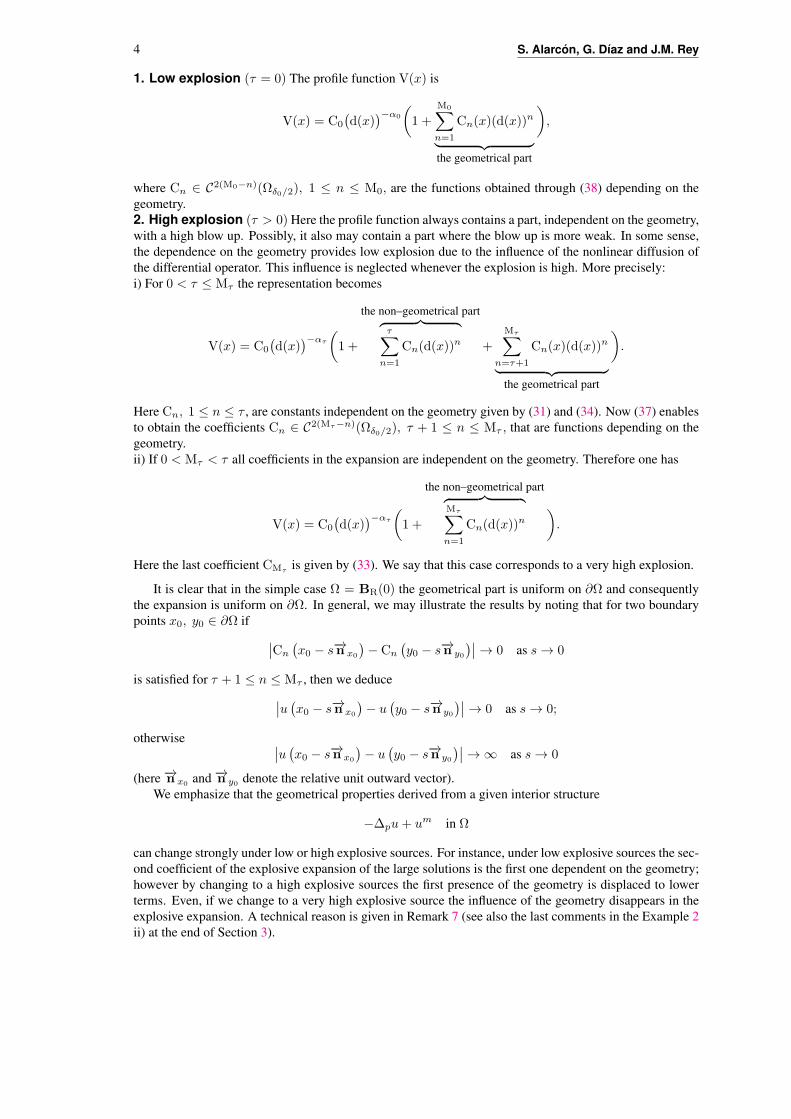
1. Low explosion (τ = 0) The profile function V(x) is
V(x) = C0
(d(x)
)−α0
(1 +
M0∑n=1
Cn(x)(d(x))n
︸ ︷︷ ︸the geometrical part
),
where Cn ∈ C2(M0−n)(Ωδ0/2), 1 ≤ n ≤ M0, are the functions obtained through (38) depending on thegeometry.2. High explosion (τ > 0) Here the profile function always contains a part, independent on the geometry,with a high blow up. Possibly, it also may contain a part where the blow up is more weak. In some sense,the dependence on the geometry provides low explosion due to the influence of the nonlinear diffusion ofthe differential operator. This influence is neglected whenever the explosion is high. More precisely:i) For 0 < τ ≤ Mτ the representation becomes
V(x) = C0
(d(x)
)−ατ
(1 +
the non–geometrical part︷ ︸︸ ︷τ∑
n=1
Cn(d(x))n +
Mτ∑n=τ+1
Cn(x)(d(x))n
︸ ︷︷ ︸the geometrical part
).
Here Cn, 1 ≤ n ≤ τ , are constants independent on the geometry given by (31) and (34). Now (37) enablesto obtain the coefficients Cn ∈ C2(Mτ−n)(Ωδ0/2), τ + 1 ≤ n ≤ Mτ , that are functions depending on thegeometry.ii) If 0 < Mτ < τ all coefficients in the expansion are independent on the geometry. Therefore one has
V(x) = C0
(d(x)
)−ατ
(1 +
the non–geometrical part︷ ︸︸ ︷Mτ∑n=1
Cn(d(x))n
).
Here the last coefficient CMτ is given by (33). We say that this case corresponds to a very high explosion.
It is clear that in the simple case Ω = BR(0) the geometrical part is uniform on ∂Ω and consequentlythe expansion is uniform on ∂Ω. In general, we may illustrate the results by noting that for two boundarypoints x0, y0 ∈ ∂Ω if ∣∣Cn
(x0 − s−→n x0
)− Cn
(y0 − s−→n y0
)∣∣ → 0 as s → 0
is satisfied for τ + 1 ≤ n ≤ Mτ , then we deduce∣∣u (x0 − s−→n x0
)− u
(y0 − s−→n y0
)∣∣ → 0 as s → 0;
otherwise ∣∣u (x0 − s−→n x0
)− u
(y0 − s−→n y0
)∣∣ → ∞ as s → 0
(here −→n x0 and −→n y0 denote the relative unit outward vector).We emphasize that the geometrical properties derived from a given interior structure
−∆pu+ um in Ω
can change strongly under low or high explosive sources. For instance, under low explosive sources the sec-ond coefficient of the explosive expansion of the large solutions is the first one dependent on the geometry;however by changing to a high explosive sources the first presence of the geometry is displaced to lowerterms. Even, if we change to a very high explosive source the influence of the geometry disappears in theexplosive expansion. A technical reason is given in Remark 7 (see also the last comments in the Example 2ii) at the end of Section 3).
The influence of sources terms on the boundary behavior of the large solutions 5
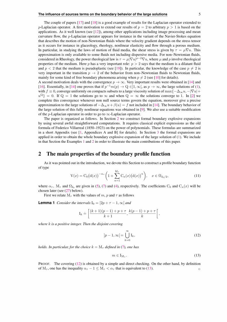
The couple of papers [17] and [18] is a good example of results for the Laplacian operator extended top-Laplacian operator. A first motivation to extend our results of p = 2 to arbitrary p > 1 is based on theapplications. As it well known (see [12]), among other applications including image processing and meancurvature flow, the p-Laplacian operator appears for instance in the variant of the Navier-Stokes equationthat describes the motion of non-Newtonian fluids where the velocity gradient depends on the stress tensoras it occurs for instance in glaceology, rheology, nonlinear elasticity and flow through a porous medium.In particular, in studying the laws of motion of fluid media, the shear stress is given by τ = µ∇u. Thisapproximation is only available to some fluids not including dispersive media. For non–Newtonian fluids,considered in Rheology, the power rheological law is τ = µ|∇u|p−2∇u, where µ and p involve rheologicalproperties of the medium. Here p has a very important role: p > 2 says that the medium is a dilatant fluidand p < 2 that the medium is pseudoplastic (see [19]). In particular, the knowledge of the case p = 2 isvery important in the transition p → 2 of the behavior from non–Newtonian fluids to Newtonian fluids,mainly for some kind of free boundary phenomena arising when p = 2 (see [10] for details).A second motivation deals with the convergence p → ∞. Very important results were obtained in [14] and[16]. Essentially, in [14] one proves that if p−1m(p) → Q ∈]1,∞[, as p → ∞, the large solutions of (1),with f ≡ 0, converge uniformly on compacts subsets to a large viscosity solution of max−∆∞u,−|∇u|+uQ = 0. If Q = 1 the solutions go to ∞ and when Q = ∞ the solutions converge to 1. In [2] wecomplete this convergence whenever non null source terms govern the equation, moreover give a preciseapproximation to the large solutions of −∆∞u+β(u) = f not included in [14]. The boundary behavior ofthe large solution of this fully nonlinear equations was obtained in [9]. We also use a suitable modificationof the p-Laplacian operator in order to go to ∞-Laplacian operator.
The paper is organized as follows. In Section 2 we construct formal boundary explosive expansionsby using several awful straightforward computations. It requires classical explicit expressions as the oldformula of Federico Villarreal (1850–1923) on the power of polynomials. These formulas are summarizedin a short Appendix (see [1, Appendices A and B] for details). In Section 3 the formal expansions areapplied in order to obtain the whole boundary explosive expansion of the large solution of (1). We includein that Section the Examples 1 and 2 in order to illustrate the main contributions of this paper.
2 The main properties of the boundary profile functionAs it was pointed out in the introduction, we devote this Section to construct a profile boundary function
of type
V(x) = C0
(d(x)
)−ατ
(1 +
Mτ∑n=1
Cn(x)(d(x)
)n), x ∈ Ωδ0/2, (11)
where ατ , Mτ and Ωδ0 are given in (5), (7) and (4), respectively. The coefficients C0 and Cn(x) will bechosen later (see (27) below).
First we relate Mτ with the values of m, p and τ as follows
Lemma 1 Consider the intervals I0 = [2p+ τ − 1,∞[ and
Ik.=
[(k + 1)(p− 1) + p+ τ
k + 1,k(p− 1) + p+ τ
k
[,
where k is a positive integer. Then the disjoint covering
]p− 1,∞[ =
∞∪k=0
Ik, (12)
holds. In particular, for the choice k = Mτ defined in (7), one has
m ∈ IMτ . (13)
PROOF. The covering (12) is obtained by a simple and direct checking. On the other hand, by definitionof Mτ , one has the inequality ατ − 1 ≤ Mτ < ατ that is equivalent to (13). 2
6 S. Alarcon, G. Dıaz and J.M. Rey
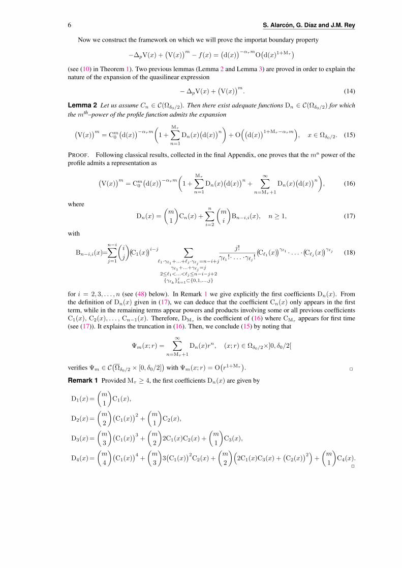
Now we construct the framework on which we will prove the importat boundary property
−∆pV(x) +(V(x)
)m − f(x) =(d(x)
)−ατmO(d(x)1+Mτ
)(see (10) in Theorem 1). Two previous lemmas (Lemma 2 and Lemma 3) are proved in order to explain thenature of the expansion of the quasilinear expression
−∆pV(x) +(V(x)
)m. (14)
Lemma 2 Let us assume Cn ∈ C(Ωδ0/2). Then there exist adequate functions Dn ∈ C(Ωδ0/2) for whichthe mth–power of the profile function admits the expansion
(V(x)
)m= Cm
0
(d(x)
)−ατm(1 +
Mτ∑n=1
Dn(x)(d(x)
)n)+O
((d(x)
)1+Mτ−ατm), x ∈ Ωδ0/2. (15)
PROOF. Following classical results, collected in the final Appendix, one proves that the mth power of theprofile admits a representation as
(V(x)
)m= Cm
0
(d(x)
)−ατm(1 +
Mτ∑n=1
Dn(x)(d(x)
)n+
∞∑n=Mτ+1
Dn(x)(d(x)
)n), (16)
where
Dn(x) =
(m
1
)Cn(x) +
n∑i=2
(m
i
)Bn−i,i(x), n ≥ 1, (17)
with
Bn−i,i(x)=n−i∑j=1
(i
j
)(C1(x)
)i−j ∑ℓ1·γℓ1
+...+ℓj ·γℓj=n−i+j
γℓ1+...+γℓj
=j
2≤ℓ1<...<ℓj≤n−i−j+2
γℓkjk=1⊂0,1,...,j
j!
γℓ1 !· . . . ·γℓj !(Cℓ1(x)
)γℓ1 · . . . ·(Cℓj (x)
)γℓj (18)
for i = 2, 3, . . . , n (see (48) below). In Remark 1 we give explicitly the first coefficients Dn(x). Fromthe definition of Dn(x) given in (17), we can deduce that the coefficient Cn(x) only appears in the firstterm, while in the remaining terms appear powers and products involving some or all previous coefficientsC1(x), C2(x), . . . , Cn−1(x). Therefore, DMτ
is the coefficient of (16) where CMτappears for first time
(see (17)). It explains the truncation in (16). Then, we conclude (15) by noting that
Ψm(x; r) =∞∑
n=Mτ+1
Dn(x)rn, (x; r) ∈ Ωδ0/2×]0, δ0/2[
verifies Ψm ∈ C(Ωδ0/2 × [0, δ0/2]
)with Ψm(x; r) = O
(r1+Mτ
). 2
Remark 1 Provided Mτ ≥ 4, the first coefficients Dn(x) are given by
D1(x)=
(m
1
)C1(x),
D2(x)=
(m
2
)(C1(x)
)2+
(m
1
)C2(x),
D3(x)=
(m
3
)(C1(x)
)3+
(m
2
)2C1(x)C2(x) +
(m
1
)C3(x),
D4(x)=
(m
4
)(C1(x)
)4+
(m
3
)3(C1(x)
)2C2(x) +
(m
2
)(2C1(x)C3(x) +
(C2(x)
)2)+
(m
1
)C4(x).
2

The influence of sources terms on the boundary behavior of the large solutions 7
The construction of the leading part of (14) is also very laborious. In particular, we have
Lemma 3 Let us assume Cn ∈ C2(Ωδ0/2). Then there exist a constant A0 and some functions An ∈C(Ωδ0/2), for which the following expansion
∆pV(x)=Cp−10
(d(x)
)−ατm(A0
(d(x)
)τ+
maxMτ−τ,0∑n=1
An(x)(d(x)
)n+τ)+O
((d(x)
)1+maxMτ ,τ−ατm)
(19)holds in Ωδ0/2.
PROOF. First of all, we obtain
∇V(x) = C0
(d(x)
)−(ατ+1)(−→A 0(x) +
Mτ∑n=1
−→An(x)
(d(x)
)n+
−→AMτ+1(x)
(d(x)
)Mτ+1)
with
−→An(x) =
−ατ∇d(x), n = 0,
(−ατ + 1)C1(x)∇d(x), n = 1,
(−ατ + n)Cn(x)∇d(x) +∇Cn−1(x), 2 ≤ n ≤ Mτ ,
∇CMτ (x), n = Mτ + 1.
(20)
Now, following again the reasonings of the Appendix, see (51), one has
|∇V(x)|2 = C20
(d(x)
)−2(ατ+1)(α2τ +
2(Mτ+1)∑n=1
En(x)(d(x)
)n), (21)
for certain functions En(x). As in (15), we focus the attention on the coefficients En(x), 1 ≤ n ≤ Mτ ,given by
En(x) =
n∑j=0
⟨−→A j(x),
−→An−j(x)⟩, 1 ≤ n ≤ Mτ (22)
(see Remark 3 where the first coefficients En(x) are detailed explicitly). Next, from (21), we may write
|∇V(x)|p−2 =(|∇V(x)|2
) p−22 = Cp−2
0
(d(x)
)−(ατ+1)(p−2)Φ
( 2(Mτ+1)∑n=1
En(x)(d(x)
)n−1)
where
Φ(s) =(α2τ + s d(x)
) p−22 = αp−2
τ
∞∑n=0
(p−22
n
)α−2nτ sn
(d(x)
)n.
As in (16), we apply the extended Villareal formula (see once again the Appendix below) in order to obtain
|∇V(x)|p−2 = Cp−20
(d(x)
)−(ατ+1)(p−2)αp−2τ
(1+
Mτ∑n=1
Fn(x)(d(x)
)n+
∞∑n=Mτ+1
Fn(x)(d(x)
)n) (23)
for x ∈ Ωδ0 , governed by
Fn(x) =
(p−22
1
)α−2τ En(x) +
n∑i=2
(p−22
i
)α−2iτ Gn−i,i(x), n ≥ 1, (24)
where
Gn−i,i(x)=n−i∑j=1
(i
j
)(E1(x)
)i−j ∑ℓ1·γℓ1
+...+ℓj ·γℓj=n−i+j
γℓ1+...+γℓj
=j
2≤ℓ1<...<ℓj≤n−i−j+2
γℓkjk=1⊂0,1,...,j
j!
γℓ1 ! · . . . · γℓj !(Eℓ1(x)
)γℓ1 · . . . ·(Eℓj (x)
)γℓj
8 S. Alarcon, G. Dıaz and J.M. Rey
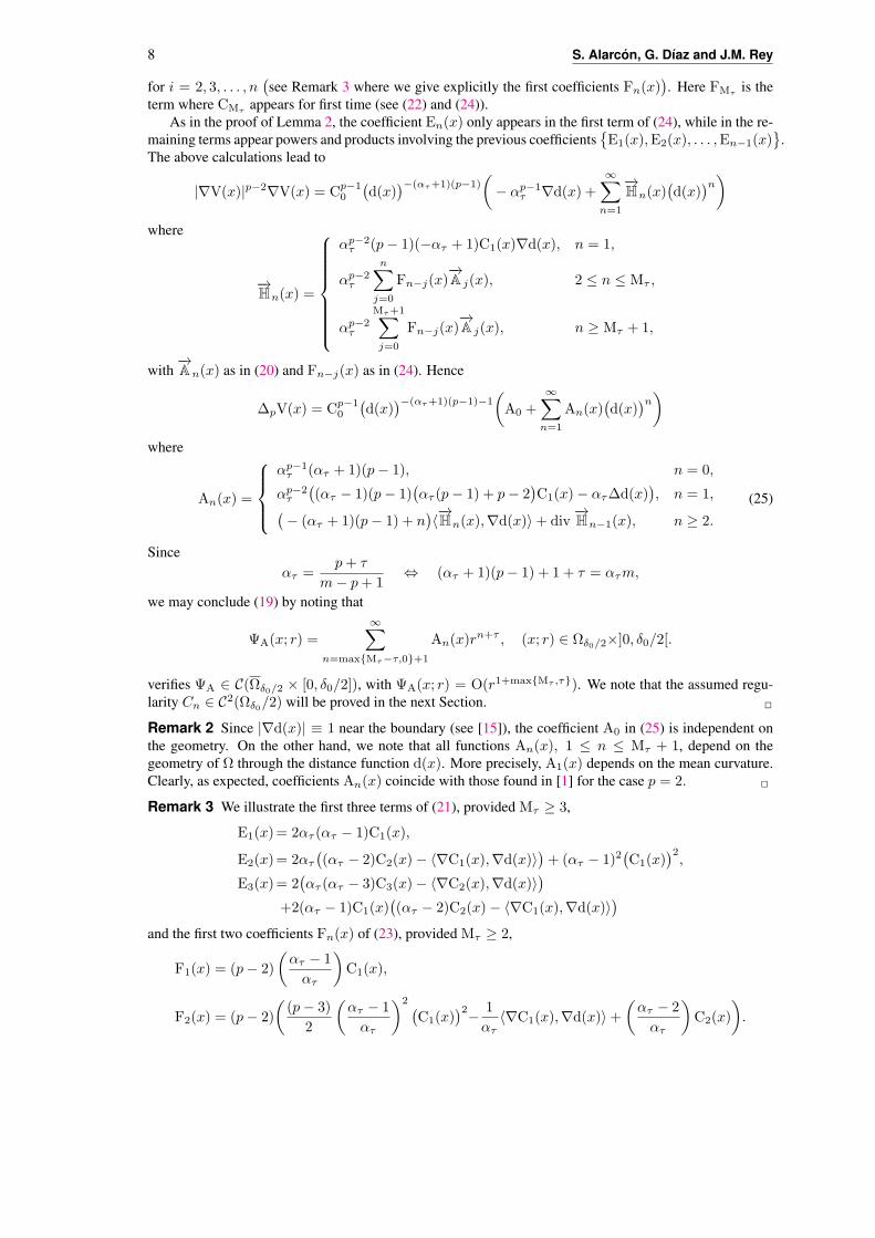
for i = 2, 3, . . . , n(see Remark 3 where we give explicitly the first coefficients Fn(x)
). Here FMτ is the
term where CMτ appears for first time (see (22) and (24)).As in the proof of Lemma 2, the coefficient En(x) only appears in the first term of (24), while in the re-
maining terms appear powers and products involving the previous coefficientsE1(x),E2(x), . . . ,En−1(x)
.
The above calculations lead to
|∇V(x)|p−2∇V(x) = Cp−10
(d(x)
)−(ατ+1)(p−1)(− αp−1
τ ∇d(x) +∞∑
n=1
−→Hn(x)
(d(x)
)n)where
−→Hn(x) =
αp−2τ (p− 1)(−ατ + 1)C1(x)∇d(x), n = 1,
αp−2τ
n∑j=0
Fn−j(x)−→A j(x), 2 ≤ n ≤ Mτ ,
αp−2τ
Mτ+1∑j=0
Fn−j(x)−→A j(x), n ≥ Mτ + 1,
with−→An(x) as in (20) and Fn−j(x) as in (24). Hence
∆pV(x) = Cp−10
(d(x)
)−(ατ+1)(p−1)−1(A0 +
∞∑n=1
An(x)(d(x)
)n)where
An(x) =
αp−1τ (ατ + 1)(p− 1), n = 0,
αp−2τ
((ατ − 1)(p− 1)
(ατ (p− 1) + p− 2
)C1(x)− ατ∆d(x)
), n = 1,(
− (ατ + 1)(p− 1) + n)⟨−→Hn(x),∇d(x)⟩+ div
−→Hn−1(x), n ≥ 2.
(25)
Sinceατ =
p+ τ
m− p+ 1⇔ (ατ + 1)(p− 1) + 1 + τ = ατm,
we may conclude (19) by noting that
ΨA(x; r) =∞∑
n=maxMτ−τ,0+1
An(x)rn+τ , (x; r) ∈ Ωδ0/2×]0, δ0/2[.
verifies ΨA ∈ C(Ωδ0/2 × [0, δ0/2]), with ΨA(x; r) = O(r1+maxMτ ,τ). We note that the assumed regu-larity Cn ∈ C2(Ωδ0/2) will be proved in the next Section. 2
Remark 2 Since |∇d(x)| ≡ 1 near the boundary (see [15]), the coefficient A0 in (25) is independent onthe geometry. On the other hand, we note that all functions An(x), 1 ≤ n ≤ Mτ + 1, depend on thegeometry of Ω through the distance function d(x). More precisely, A1(x) depends on the mean curvature.Clearly, as expected, coefficients An(x) coincide with those found in [1] for the case p = 2. 2
Remark 3 We illustrate the first three terms of (21), provided Mτ ≥ 3,
E1(x)= 2ατ (ατ − 1)C1(x),
E2(x)= 2ατ
((ατ − 2)C2(x)− ⟨∇C1(x),∇d(x)⟩
)+ (ατ − 1)2
(C1(x)
)2,
E3(x)= 2(ατ (ατ − 3)C3(x)− ⟨∇C2(x),∇d(x)⟩
)+2(ατ − 1)C1(x)
((ατ − 2)C2(x)− ⟨∇C1(x),∇d(x)⟩
)and the first two coefficients Fn(x) of (23), provided Mτ ≥ 2,
F1(x) = (p− 2)
(ατ − 1
ατ
)C1(x),
F2(x) = (p− 2)
((p− 3)
2
(ατ − 1
ατ
)2 (C1(x)
)2− 1
ατ⟨∇C1(x),∇d(x)⟩+
(ατ − 2
ατ
)C2(x)
).
The influence of sources terms on the boundary behavior of the large solutions 9
Obviously, equality (23) is irrelevant when p = 2 because Fn(x), 1 ≤ n ≤ Mτ , are null functions. 2
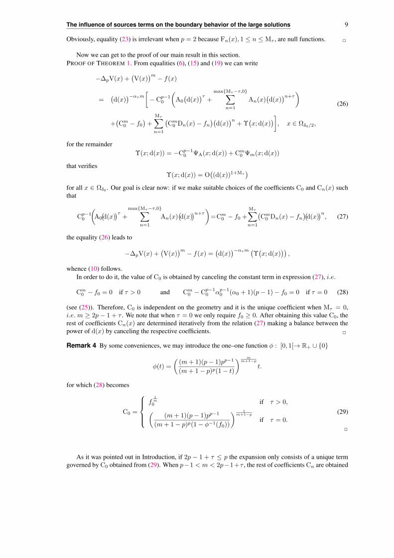
Now we can get to the proof of our main result in this section.PROOF OF THEOREM 1. From equalities (6), (15) and (19) we can write
−∆pV(x) +(V(x)
)m − f(x)
=(d(x)
)−ατm[− Cp−1
0
(A0
(d(x)
)τ+
maxMτ−τ,0∑n=1
An(x)(d(x)
)n+τ)
+(Cm
0 − f0)+
Mτ∑n=1
(Cm
0 Dn(x)− fn)(d(x)
)n+Υ
(x; d(x)
)], x ∈ Ωδ0/2,
(26)
for the remainderΥ(x; d(x)) = −Cp−1
0 ΨA(x; d(x)) + Cm0 Ψm(x; d(x))
that verifiesΥ(x; d(x)) = O
((d(x))1+Mτ
)for all x ∈ Ωδ0 . Our goal is clear now: if we make suitable choices of the coefficients C0 and Cn(x) suchthat
Cp−10
(A0
(d(x)
)τ+
maxMτ−τ,0∑n=1
An(x)(d(x)
)n+τ)=Cm
0 − f0 +
Mτ∑n=1
(Cm
0 Dn(x)− fn)(d(x)
)n, (27)
the equality (26) leads to
−∆pV(x) +(V(x)
)m − f(x) =(d(x)
)−ατm (Υ(x; d(x)
)),
whence (10) follows.In order to do it, the value of C0 is obtained by canceling the constant term in expression (27), i.e.
Cm0 − f0 = 0 if τ > 0 and Cm
0 − Cp−10 αp−1
0 (α0 + 1)(p− 1)− f0 = 0 if τ = 0 (28)
(see (25)). Therefore, C0 is independent on the geometry and it is the unique coefficient when Mτ = 0,i.e. m ≥ 2p− 1 + τ . We note that when τ = 0 we only require f0 ≥ 0. After obtaining this value C0, therest of coefficients Cn(x) are determined iteratively from the relation (27) making a balance between thepower of d(x) by canceling the respective coefficients. 2
Remark 4 By some conveniences, we may introduce the one–one function ϕ : [0, 1[→ R+ ∪ 0
ϕ(t) =
((m+ 1)(p− 1)pp−1
(m+ 1− p)p(1− t)
) mm+1−p
t.
for which (28) becomes
C0 =
f
1m0 if τ > 0,(
(m+ 1)(p− 1)pp−1
(m+ 1− p)p(1− ϕ−1(f0))
) 1m+1−p
if τ = 0.(29)
2
As it was pointed out in Introduction, if 2p − 1 + τ ≤ p the expansion only consists of a unique termgoverned by C0 obtained from (29). When p−1 < m < 2p−1+τ , the rest of coefficients Cn are obtained
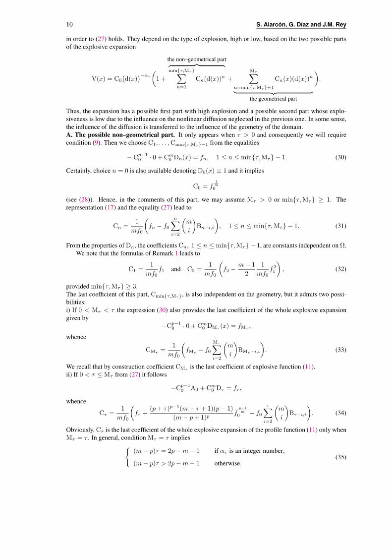
10 S. Alarcon, G. Dıaz and J.M. Rey
in order to (27) holds. They depend on the type of explosion, high or low, based on the two possible partsof the explosive expansion
V(x) = C0
(d(x)
)−ατ
(1 +
the non–geometrical part︷ ︸︸ ︷minτ,Mτ∑
n=1
Cn(d(x))n +
Mτ∑n=minτ,Mτ+1
Cn(x)(d(x))n
︸ ︷︷ ︸the geometrical part
).
Thus, the expansion has a possible first part with high explosion and a possible second part whose explo-siveness is low due to the influence on the nonlinear diffusion neglected in the previous one. In some sense,the influence of the diffusion is transferred to the influence of the geometry of the domain.A. The possible non–geometrical part. It only appears when τ > 0 and consequently we will requirecondition (9). Then we choose C1, . . . ,Cminτ,Mτ−1 from the equalities
− Cp−10 · 0 + Cm
0 Dn(x) = fn, 1 ≤ n ≤ minτ,Mτ − 1. (30)
Certainly, choice n = 0 is also available denoting D0(x) ≡ 1 and it implies
C0 = f1m0
(see (28)). Hence, in the comments of this part, we may assume Mτ > 0 or minτ,Mτ ≥ 1. Therepresentation (17) and the equality (27) lead to
Cn =1
mf0
(fn − f0
n∑i=2
(m
i
)Bn−i,i
), 1 ≤ n ≤ minτ,Mτ − 1. (31)
From the properties of Dn, the coefficients Cn, 1 ≤ n ≤ minτ,Mτ −1, are constants independent on Ω.We note that the formulas of Remark 1 leads to
C1 =1
mf0f1 and C2 =
1
mf0
(f2 −
m− 1
2
1
mf0f21
), (32)
provided minτ,Mτ ≥ 3.The last coefficient of this part, Cminτ,Mτ, is also independent on the geometry, but it admits two possi-bilities:i) If 0 < Mτ < τ the expression (30) also provides the last coefficient of the whole explosive expansiongiven by
−Cp−10 · 0 + Cm
0 DMτ (x) = fMτ ,
whence
CMτ =1
mf0
(fMτ − f0
Mτ∑i=2
(m
i
)BMτ−i,i
). (33)
We recall that by construction coefficient CMτ is the last coefficient of explosive function (11).ii) If 0 < τ ≤ Mτ from (27) it follows
−Cp−10 A0 +Cm
0 Dτ = fτ ,
whence
Cτ =1
mf0
(fτ +
(p+ τ)p−1(m+ τ + 1)(p− 1)
(m− p+ 1)pf
p−1m
0 − f0
τ∑i=2
(m
i
)Bτ−i,i
). (34)
Obviously, Cτ is the last coefficient of the whole explosive expansion of the profile function (11) only whenMτ = τ . In general, condition Mτ = τ implies
(m− p)τ = 2p−m− 1 if ατ is an integer number,
(m− p)τ > 2p−m− 1 otherwise.(35)
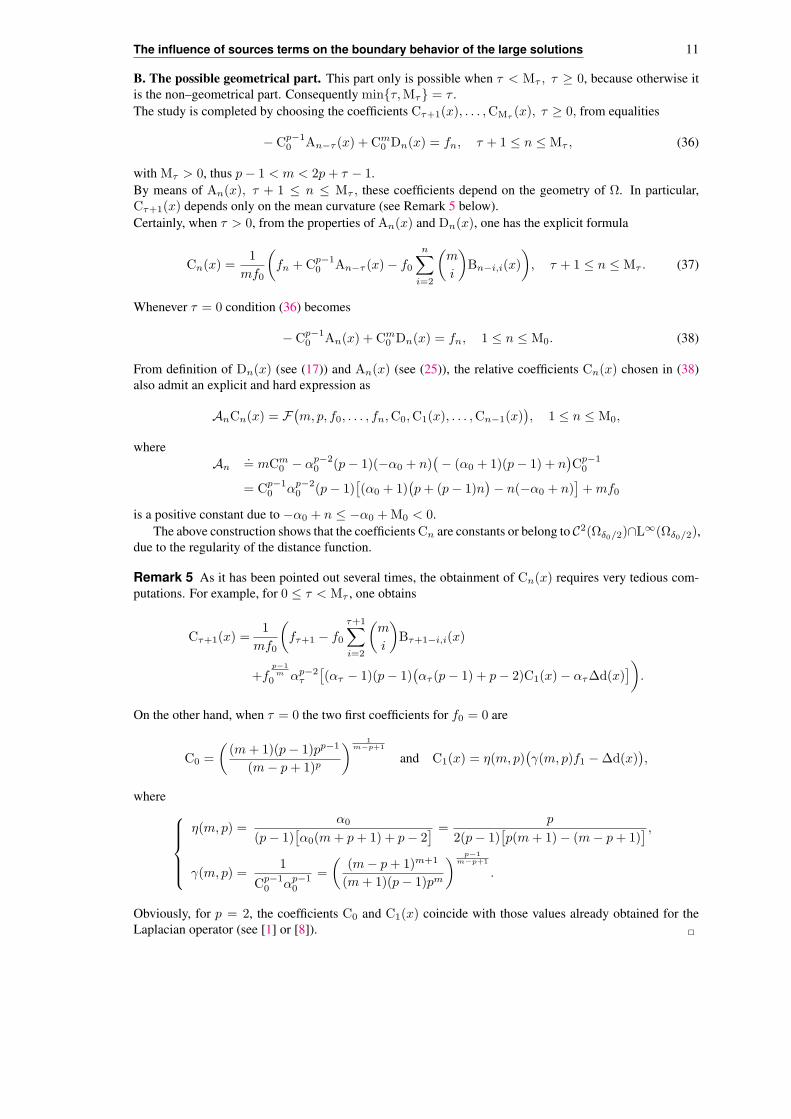
The influence of sources terms on the boundary behavior of the large solutions 11
B. The possible geometrical part. This part only is possible when τ < Mτ , τ ≥ 0, because otherwise itis the non–geometrical part. Consequently minτ,Mτ = τ .The study is completed by choosing the coefficients Cτ+1(x), . . . ,CMτ (x), τ ≥ 0, from equalities
− Cp−10 An−τ (x) + Cm
0 Dn(x) = fn, τ + 1 ≤ n ≤ Mτ , (36)
with Mτ > 0, thus p− 1 < m < 2p+ τ − 1.By means of An(x), τ + 1 ≤ n ≤ Mτ , these coefficients depend on the geometry of Ω. In particular,Cτ+1(x) depends only on the mean curvature (see Remark 5 below).Certainly, when τ > 0, from the properties of An(x) and Dn(x), one has the explicit formula
Cn(x) =1
mf0
(fn +Cp−1
0 An−τ (x)− f0
n∑i=2
(m
i
)Bn−i,i(x)
), τ + 1 ≤ n ≤ Mτ . (37)
Whenever τ = 0 condition (36) becomes
− Cp−10 An(x) + Cm
0 Dn(x) = fn, 1 ≤ n ≤ M0. (38)
From definition of Dn(x) (see (17)) and An(x) (see (25)), the relative coefficients Cn(x) chosen in (38)also admit an explicit and hard expression as
AnCn(x) = F(m, p, f0, . . . , fn,C0,C1(x), . . . ,Cn−1(x)
), 1 ≤ n ≤ M0,
whereAn
.= mCm
0 − αp−20 (p− 1)(−α0 + n)
(− (α0 + 1)(p− 1) + n
)Cp−1
0
= Cp−10 αp−2
0 (p− 1)[(α0 + 1)
(p+ (p− 1)n
)− n(−α0 + n)
]+mf0
is a positive constant due to −α0 + n ≤ −α0 +M0 < 0.The above construction shows that the coefficients Cn are constants or belong to C2(Ωδ0/2)∩L∞(Ωδ0/2),
due to the regularity of the distance function.
Remark 5 As it has been pointed out several times, the obtainment of Cn(x) requires very tedious com-putations. For example, for 0 ≤ τ < Mτ , one obtains
Cτ+1(x) =1
mf0
(fτ+1 − f0
τ+1∑i=2
(m
i
)Bτ+1−i,i(x)
+fp−1m
0 αp−2τ
[(ατ − 1)(p− 1)
(ατ (p− 1) + p− 2)C1(x)− ατ∆d(x)
]).
On the other hand, when τ = 0 the two first coefficients for f0 = 0 are
C0 =
((m+ 1)(p− 1)pp−1
(m− p+ 1)p
) 1m−p+1
and C1(x) = η(m, p)(γ(m, p)f1 −∆d(x)
),
where η(m, p) =
α0
(p− 1)[α0(m+ p+ 1) + p− 2
] =p
2(p− 1)[p(m+ 1)− (m− p+ 1)
] ,γ(m, p) =
1
Cp−10 αp−1
0
=
((m− p+ 1)m+1
(m+ 1)(p− 1)pm
) p−1m−p+1
.
Obviously, for p = 2, the coefficients C0 and C1(x) coincide with those values already obtained for theLaplacian operator (see [1] or [8]). 2
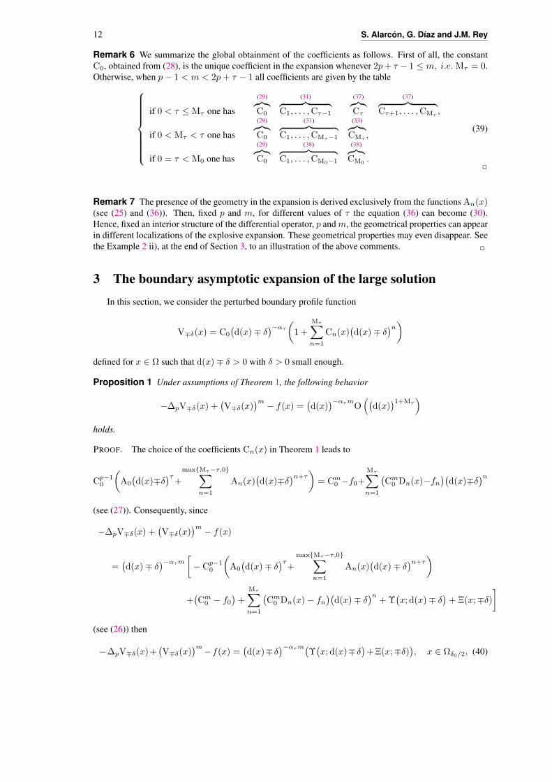
12 S. Alarcon, G. Dıaz and J.M. Rey
Remark 6 We summarize the global obtainment of the coefficients as follows. First of all, the constantC0, obtained from (28), is the unique coefficient in the expansion whenever 2p+ τ − 1 ≤ m, i.e.Mτ = 0.Otherwise, when p− 1 < m < 2p+ τ − 1 all coefficients are given by the table
if 0 < τ ≤ Mτ one has
(29)︷︸︸︷C0
(31)︷ ︸︸ ︷C1, . . . ,Cτ−1
(37)︷︸︸︷Cτ
(37)︷ ︸︸ ︷Cτ+1, . . . ,CMτ ,
if 0 < Mτ < τ one has
(29)︷︸︸︷C0
(31)︷ ︸︸ ︷C1, . . . ,CMτ−1
(33)︷︸︸︷CMτ ,
if 0 = τ < M0 one has
(29)︷︸︸︷C0
(38)︷ ︸︸ ︷C1, . . . ,CM0−1
(38)︷︸︸︷CM0
.
(39)
2
Remark 7 The presence of the geometry in the expansion is derived exclusively from the functions An(x)(see (25) and (36)). Then, fixed p and m, for different values of τ the equation (36) can become (30).Hence, fixed an interior structure of the differential operator, p and m, the geometrical properties can appearin different localizations of the explosive expansion. These geometrical properties may even disappear. Seethe Example 2 ii), at the end of Section 3, to an illustration of the above comments. 2
3 The boundary asymptotic expansion of the large solutionIn this section, we consider the perturbed boundary profile function
V∓δ(x) = C0
(d(x)∓ δ
)−ατ
(1 +
Mτ∑n=1
Cn(x)(d(x)∓ δ
)n)defined for x ∈ Ω such that d(x)∓ δ > 0 with δ > 0 small enough.
Proposition 1 Under assumptions of Theorem 1, the following behavior
−∆pV∓δ(x) +(V∓δ(x)
)m − f(x) =(d(x)
)−ατmO((
d(x))1+Mτ
)holds.
PROOF. The choice of the coefficients Cn(x) in Theorem 1 leads to
Cp−10
(A0
(d(x)∓δ
)τ+
maxMτ−τ,0∑n=1
An(x)(d(x)∓δ
)n+τ)
= Cm0 −f0+
Mτ∑n=1
(Cm
0 Dn(x)−fn)(d(x)∓δ
)n(see (27)). Consequently, since
−∆pV∓δ(x) +(V∓δ(x)
)m − f(x)
=(d(x)∓ δ
)−ατm[− Cp−1
0
(A0
(d(x)∓ δ
)τ+
maxMτ−τ,0∑n=1
An(x)(d(x)∓ δ
)n+τ)
+(Cm
0 − f0)+
Mτ∑n=1
(Cm
0 Dn(x)− fn)(d(x)∓ δ
)n+Υ
(x; d(x)∓ δ
)+ Ξ(x;∓δ)
](see (26)) then
−∆pV∓δ(x)+(V∓δ(x)
)m−f(x) =(d(x)∓δ
)−ατm(Υ(x; d(x)∓δ
)+Ξ(x;∓δ)
), x ∈ Ωδ0/2, (40)

The influence of sources terms on the boundary behavior of the large solutions 13
for the remaindersΥ(x; d(x)∓ δ) = −Cp−1
0 ΨA(x; d(x)∓ δ) + Cm0 Ψm(x; d(x)∓ δ),
Ξ(x;∓δ) =
(f0 +
Mτ∑n=1
fn(d(x)∓ δ
)n)−(d(x)∓ δ
d(x)
)ατm (f0 +
Mτ∑n=1
fn(d(x)
)n),
(41)
that verifylimδ→0
Υ(x; d(x)∓ δ) = O((d(x))1+Mτ
)and lim
δ→0Ξ(x;∓δ) = 0
for all x ∈ Ωδ0 . 2
For future purposes it will be very useful to rewrite (40) as
−∆pV∓δ(x)+(V∓δ(x)
)m − f(x) =(d(x)∓ δ
)−ατm(Pτ (C0)+Υ
(x; d(x)∓ δ
)+Ξ(x;∓δ)
))(42)
due to C0 is the positive root of polynomial
Pτ (µ) =
µm − αp−1
0 (α0 + 1)(p− 1)µp−1 − f0 if τ = 0,
µm − f0 if τ > 0,
(see (28)).
With all previous results, we get to the proof of our main result.PROOF OF THEOREM 2. In order to apply a comparison argument, we consider the modifications
W∓δ,±ε(x) = C0
(d(x)∓ δ
)−ατ
(1± ε+
Mτ∑n=1
Cn(x)(d(x)∓ δ
)n),
where ε > 0 will be sent to 0. So, we construct the perturbed polynomials
Pτ,±ε(µ) =
((1± ε)µ
)m − αp−10 (α0 + 1)(p− 1)
((1± ε)µ
)p−1 − f0 if τ = 0,((1± ε)µ
)m − f0 if τ > 0,
for whichPτ,+ε(C0) > 0 and Pτ,−ε(C0) < 0.
The reasoning is based on to prove that the functions W−δ,+ε(x) and W+δ,−ε(x) are respectively super andsubsolutions in a thin strip near the boundary. Arguing as in Theorem 1, we have
−∆pW−δ,+ε(x)+(W−δ,+ε(x)
)m−f(x) =(d(x)− δ
)−ατm(Pτ,+ε(C0)+Υ
(x; d(x)− δ
)+Ξ(x;−δ)
)(see (42)). We recall that Pτ,+ε(C0) is a positive constant independent on x and δ, consequently (41) provesthe inequality
Pτ,+ε(C0) + Υ(x; d(x)− δ
)+ Ξ(x;−δ) > 0
in a parallel strip δ < d(x) < δ1, provided 2δ1 < δ0 small enough. Therefore, the inequality
−∆pW−δ,+ε(x) +(W−δ,+ε(x)
)m> f(x), δ < d(x) < δ1,
holds. Then, Comparison Principle leads to
u(x)−W−δ,+ε(x) ≤ supd(y)=δ1
(u(y)−W−δ,+ε(y)
), δ < d(x) < δ1
or
u(x)
W−δ,+ε(x)− 1 ≤
supd(y)=δ1
(u(y)−W−δ,+ε(y)
)W−δ,+ε(x)
, δ < d(x) < δ1.

14 S. Alarcon, G. Dıaz and J.M. Rey
Now, in short, sending δ1 → 0 and then ε → 0, we deduce
lim supd(x)→0
u(x)
V(x)≤ 1,
where V is our master function given by (8). (In fact, for a more precise way to obtain this inequality wesend δ → 0, after d(x) → 0, next δ1 → 0 and finally ε → 0.)Analogously, one obtains
−∆pW+δ,−ε(x)+(W+δ,−ε(x)
)m−f(x) =(d(x)+δ
)−ατm(Pτ,−ε(C0)+Υ
(x; d(x)+δ
)+Ξ(x; +δ)
).
SincePτ,−ε(C0) + Υ
(x; d(x) + δ
)+ Ξ(x; +δ) < 0
in a parallel strip 0 < d(x) < δ1, provided 2δ1 < δ0 small enough, inequality
−∆pW+δ,−ε(x) +(W+δ,−ε(x)
)m< f(x), 0 < d(x) < δ1,
holds. Now, by comparing, it follows
1− u(x)
W+δ,−ε(x)≤
supd(y)=δ1
(W+δ,−ε(y)− u(y)
)W+δ,−ε(x)
, 0 < d(x) < δ1.
As above, sending δ → 0 and then ε → 0, we conclude
lim supd(x)→0
u(x)
V(x)≤ 1 ≤ lim inf
d(x)→0
u(x)
V(x).
2
Remark 8 Certainly Theorem 2 extends and generalizes Theorem 3.8 of [11]. When p = 2 Theorem 2coincides with Theorem 2 of [1] and it extends the results obtained in [5], [6] or [8] where only the secondexplosive term was considered for f ≡ 0. 2
Theorem 2 can be illustrated as follows
Example 1 (Low explosive sources) This is an example without non diffused part in the expansionof the large solutions. For instance, let us suppose
3p− 2
2≤ m < 2p− 1 (43)
(or equivalently 1 < α0 ≤ 2), for which M0 = 1 and
f(x) = f1(d(x)
)− pmm−p+1+1
, f1 ≥ 0.
If ∂Ω ∈ C4, then we obtain
u(x) = C0
(d(x)
)− pm−p+1
(1 + η(m, p)
[γ(m, p)f1 −∆d(x)
]d(x)
)+ o
((d(x)
)m−2p+1m−p+1
), (44)
where C0, η(m, p) and γ(m, p) are given in Remark 5. This example extends the results of [5], [6] or [8]obtained for p = 2 and f ≡ 0. 2
Example 2 (High explosive sources)
i) In order to simplify, we begin by constructing an example without geometrical part in the expansion. Forinstance, the equality τ = Mτ requires
p(2 + τ)− 1
τ + 1< m and m ∈ IMτ

The influence of sources terms on the boundary behavior of the large solutions 15
see (35) and Lemma 1. In particular, for the choice τ = 1 both conditions hold when
3p
2< m < 2p.
Then, let us considerf(x) =
(d(x)
)−α1m(f0 + f1d(x)
), f0 > 0
whereα1 =
p+ 1
m− p+ 1
verifies
1 < α1 <2(p+ 1)
p+ 2.
Theorem 2 proves that the expansion of all explosive terms of the large solution is
u(x) = f1m0
(d(x)
)−α1
(1 +
1
mf0
(f1 +
(p+ 1)p−1(m+ 2)(p− 1)
(m− p+ 1)pf
p−1m
0
)d(x)
)+ o
((d(x)
)−α1+1),
provided ∂Ω ∈ C4 (see (5), (32), (34) and (35)). Clearly, both coefficients are independent on the geometryof Ω.
ii) Finally, we construct an example where the expansion has one coefficient dependent on Ω plus twocoefficients uniform and independent on Ω; therefore τ = 1 and M1 + 1 = 3. So, Lemma 1 enables us toconsider
4p− 2
3≤ m <
3p− 1
2(45)
(or equivalently 2 < α1 ≤ 3) and, for simplicity, we suppose
f(x) = f0(d(x)
)− (p+1)mm−p+1
(1 + f1d(x) + f2
(d(x)
)2), f0 > 0.
Then the expansion of all explosive terms of the large solution is
u(x) = C0
(d(x)
)− p+1m−p+1
(1 + C1d(x) + C2(x)
(d(x)
)2)+ o
((d(x)
) 2m−3p+1m−p+1
), (46)
for coefficients
C0 = f1m0 (independent on the nonlinear diffusion)
C1 =1
mf0
(f1 + αp−1
1 (α1 + 1)(p− 1)fp−1m
0
)(dependent on the nonlinear diffusion)
and
C2(x) =1
mf0
(f2−f0
m(m− 1)
2C2
1+fp−1m
0 αp−21
((α1−1)(p−1)(α1(p−1)+p−2)C1−α1∆d(x)
)),
where α1 =p+ 1
m− p+ 1provided ∂Ω ∈ C6 (see Remarks 1 and 5).
One last comment derived from conditions (43) and (45). Since3p− 1
2< 2p− 1,
3p− 2
2<
4p− 2
3, provided 1 < p < 2,
implies the inclusion[4p− 2
3,3p− 1
2
[⊆
[3p− 2
2, 2p− 1
[, provided 1 < p < 2,

16 S. Alarcon, G. Dıaz and J.M. Rey
we note that for every
m ∈[4p− 2
3,3p− 1
2
[, 1 < p < 2,
and ∂Ω ∈ C4, the first geometrical property appears in the coefficient C1(x) of the expansion for the lowexplosion source
f(x) = f1(d(x)
)− pmm−p+1+1
, f1 ≥ 0
(see (44)). However, if ∂Ω ∈ C6 and we change to the high explosion source
f(x) = f0(d(x)
)− (p+1)mm−p+1
(1 + f1d(x) + f2
(d(x)
)2), f0 > 0,
that first geometrical property appears now in the C2(x) coefficient (see (46)), while the coefficient C1 isindependent n the geometry. The importance of the kind of sources was commented in Remark 7. 2
Appendix: Expanding the mth power of the asymptotic profileIn Appendix A of [1] the old formula of Federico Villarreal (1850–1923) on the power of polynomials
was extended by means of an explicit expression. It was applied in order to obtain representations of thepower of polynomials. Here we sketch the results of Appendix B of [1] related to the formal expansion
V(x) = C0
(d(x)
)−ατ
(1 +
Mτ∑n=1
Cn(x)(d(x)
)n)for which (
V(x))m
= Cm0
(d(x)
)−ατmΦ
( Mτ∑n=1
Cn(x)(d(x)
)n−1),
whereΦ(s) =
(1 + sd(x)
)m.
Applying Taylor expansion of Φ(s) one obtains
(V(x)
)m= Cm
0
(d(x)
)−ατm∑n≥0
(m
n
)( Mτ∑k=1
Ck(x)(d(x)
)k−1)n(
d(x))n
.
On the other hand, we may write
( Mτ∑k=1
Ck(x)(d(x)
)k−1)n
=
(Mτ−1∑k=0
Ck+1(x)(d(x)
)k)n
=
(Mτ−1)n∑i=0
Bi,n(x)(d(x)
)i(47)
where
Bi,n(x) =
(C1(x)
)n, i = 0,
1
iC1(x)
i−1∑ℓ=0
((i− ℓ)(n+ 1)− i
)Ci−ℓ+1(x)Bℓ,n(x), 1 ≤ i ≤ Mτ − 1,
1
iC1(x)
i−1∑ℓ=i−Mτ+1
((i− ℓ)(n+ 1)− i
)Ci−ℓ+1(x)Bℓ,n(x), Mτ ≤ i ≤ (Mτ − 1)n
(for details see [1, Appendix A]).In general, by means of a transfinite induction argument we may adjust explicit Villarreal formula (see
now [1, Theorem 4]) in order to obtain the explicit expression of Bi,n(x) for i ∈ 1, 2, . . . , n (see also

The influence of sources terms on the boundary behavior of the large solutions 17
(18)). Then one has
(V(x)
)m= Cm
0
(d(x)
)−ατm∑n≥0
(m
n
) (Mτ−1)n∑i=0
Bi,n(x)(d(x)
)i+n
= Cm0
(d(x)
)−ατm(1 +
∞∑n=1
Dn(x)(d(x)
)n) (48)
where
Dn(x) =n∑
i=1
(m
i
)Bn−i,i(x), for all n. (49)
Choosing n = 1 in (47) we deduce
Bi,1(x) = Ci+1(x), 0 ≤ i ≤ Mτ−1,
so that, (49) becomes
Dn(x) =
(m
1
)Cn(x) +
n∑i=2
(m
i
)Bn−i,i(x), 1 ≤ n ≤ Mτ , (50)
whence, in (50), each Cn(x), 1 ≤ n ≤ Mτ , does not appear in Bn−i,i(x), i = 1. Certainly all coefficientsCn(x), 1 ≤ n ≤ Mτ , are involved in the other Dn(x), n ≥ Mτ + 1.Clearly, the Taylor expansion is finite when m is an integer number. In this case, representation (48)becomes (
V(x))m
= Cm0
(d(x)
)−ατm(1 +
m(Mτ−1)∑n=1
Dn(x)(d(x)
)n) (51)
where coefficients Dn(x) are given in (49).
References[1] Alarcon, S., Dıaz, G., Letelier, R. and Rey, J.M.: Expanding the asymptotic explosive boundary
behavior of large solutions to a semilinear elliptic equation, Nonlinear Analysis 72, (2010), 2426–2443.
[2] Alarcon, S., Dıaz, G. and Rey, J.M.: On the large solutions of a class of fully nonlinear degenerateelliptic equations and some approximations problems, work in progress.
[3] Anneda, C. and Porru, G.: Higher order boundary estimate for blow–up solutions of elliptic equations,Differential Integral Equations, 3 (19), (2006), 345–360.
[4] Anneda, C. and Porru, G.: Second order estimates for boundary blow–up solutions of elliptic equa-tions, Discrete Contin. Dyn. Syst., Proceedings of the 6th AIMS International Conference, suppl.,(2007), 54–63.
[5] Bandle, C.: Asymptotic behavior of large solutions of elliptic equations, Annals of University ofCraiova, Math. Comp. Sci. Ser., 2, (2005), 1–8.
[6] Bandle, C. and Marcus, M.: Dependence of blowup rate of large solutions of semilinear elliptic equa-tions, on the curvature of the boundary, Complex Variables Theory Appl., 49, (2004), 555–570.
[7] Berhanu, S. and Porru, G.: Qualitative and quantitative estimate for large solutions to semilinearequations, Commun. Appl. Anal., 4, (1), (2000), 121–131.
[8] Del Pino, M. and Letelier, R.: The influence of domain geometry in boundary blow–up elliptic prob-lems, Nonlinear Anal., 48 (6), (2002), 897–904.

18 S. Alarcon, G. Dıaz and J.M. Rey
[9] Dıaz, G. and Dıaz, J.I.: Uniqueness of the boundary behavior for large solutions to a degenerateelliptic equation involving the ∞–Laplacian, RACSAM Rev. R. Acad. Cienc. Serie A Mat., 97 (3)(2003), 455–460.
[10] Dıaz, G. and Dıaz, J.I.: On different Darcy laws, from non-Newtonian to Newtonian fluids: a mathe-matical point of view, work in progress.
[11] Dıaz, G. and Letelier, R.: Explosive solutions of quasilinear elliptic equations: existence and unique-ness, Nonlinear Anal., 20 (2), (1993), 97–125.
[12] Dıaz, J.I.: Nonlinear Partial Differential Equations and Free Boundaries, Vol. 1 Elliptic Equations,Res. Notes Math, 106. Pitman, 1985.
[13] Gladiali, F. and Porru, G.: Estimates for explosive solutions to p-Laplace equations, Progress in PartialDifferential Equations, (Pont-a-Mousson 1997), Vol. 1, Pitman Res. Notes Math.
[14] Garcıa–Melian, J., Rossi, J. D. and Sabina, J.: Large solutions to the p-Laplacian for large p, Calculusof Variations and Partial Differential Equations, 31(2), (2008), 187–204.
[15] Gilbarg, D. and Trudinger, N.: Elliptic Partial Differential Equations of Second Order. Springer–Verlag (1983).
[16] Juutinen, P., Lindqvist, P. and Manfredi, J.: The ∞-eigenvalue problem, Arch. Rat. Mech. Anal. , 148(1999), 89-105.
[17] Lieberman, G.M.; Asymptotic behavior and uniqueness of blow-up solutions of elliptic equations,Methods Appl. Anal., 15 (2008), 243–262.
[18] Lieberman, G.M.: Asymptotic behavior and uniqueness of blow-up solutions of quasilinear ellipticequations, J. Anal. Math., 115 (2011), 213–249.
[19] Malkin, A.Y. and Isayev, A.I.: Rheology: concepts, methods, & applications, Toronto ChemTec Pub-lishing, 2006.
[20] Marcus, M. and Veron, L.: Maximal solutions of semilinear elliptic equations with locally integrableforcing term, Israel J. Math., 152, (2006), 333–348.
[21] Matero J.: Quasilinear elliptic equations with boundary blow-up, J. d’Anal. Math., 96, (1996), 229–247.
[22] Radulescu, V.: Singular phenomena in nonlinear elliptic problems: from boundary blow-up solutionsto equations with singular nonlinearities, in Handbook of Differential Equations: Stationary PartialDifferential Equations, Vol. 4 (Michel Chipot, Editor) (2007), 483–591.
[23] Veron, L.: Semilinear elliptic equations with uniform blow-up on the boundary. Festschrift on theoccasion of the 70th birthday of Shmuel Agmon. J. Anal. Math., 59 (1992), 231–250.
[24] Zhang, Z.: A boundary blow-up elliptic problem with an inhomogeneous term, Nonlinear Analysis,68 (2008), 3428-3438.
S. Alarcon G. Dıaz J. M. ReyDpto. de Matematica Dpto. de Matematica Aplicada Dpto. de Matematica AplicadaU. Tecnica Federico Santa Marıa U. Complutense de Madrid U. Complutense de MadridCasilla 110-V Valparaıso Chile. 28040 Madrid, Spain 28040 Madrid, [email protected] [email protected] [email protected]

PREPUBLICACIONES DEL DEPARTAMENTODE MATEMÁTICA APLICADA
UNIVERSIDAD COMPLUTENSE DE MADRIDMA-UCM 2011
1. APPROXIMATING TRAVELLING WAVES BY EQUILIBRIA OF NON LOCAL EQUATIONS, J. M. Arrieta, M. López-Fernández and E. Zuazua.
2. INFINITELY MANY STABILITY SWITCHES IN A PROBLEM WITH SUBLINEAR OSCILLATORY BOUNDARY CONDITIONS, A. Castro and R. Pardo
3. THIN DOMAINS WITH EXTREMELY HIGH OSCILLATORY BOUNDARIES, J. M. Arrieta and M. C. Pereira
4. FROM NEWTON EQUATION TO FRACTIONAL DIFFUSION AND WAVE EQUATIONS, L. Váquez
5. EL CÁLCULO FRACCIONARIO COMO INSTRUMENTO DE MODELIZACIÓN, L. Váquez and M. P. Velasco
6. THE TANGENTIAL VARIATION OF A LOCALIZED FLUX-TYPE EIGENVALUE PROBLEM, R. Pardo, A. L. Pereira and J. C. Sabina de Lis
7. IDENTIFICATION OF A HEAT TRANSFER COEFFICIENT DEPENDING ON PRESSURE AND TEMPERATURE, A. Fraguela, J. A. Infante, Á. M. Ramos and J. M. Rey
8. A NOTE ON THE LIOUVILLE METHOD APPLIED TO ELLIPTIC EVENTUALLY DEGENERATE FULLY NONLINEAR EQUATIONS GOVERNED BY THE PUCCI OPERATORS AND THE KELLER–OSSERMAN CONDITION, G. Díaz
9. RESONANT SOLUTIONS AND TURNING POINTS IN AN ELLIPTIC PROBLEM WITH OSCILLATORY BOUNDARY CONDITIONS, A. Castro and R. Pardo
10. BE-FAST: A SPATIAL MODEL FOR STUDYING CLASSICAL SWINE FEVER VIRUS SPREAD BETWEEN AND WITHIN FARMS. DESCRIPTION AND VALIDATION. B. Ivorra B. Martínez-López, A. M. Ramos and J.M. Sánchez-Vizcaíno.
11. FRACTIONAL HEAT EQUATION AND THE SECOND LAW OF THERMODYNAMICS, L. Vázquez , J. J. Trujillo and M. P. Velasco
12. LINEAR AND SEMILINEAR HIGHER ORDER PARABOLIC EQUATIONS IN R^N, J. Cholewa and A. Rodríguez Bernal
13. DISSIPATIVE MECHANISM OF A SEMILINEAR HIGHER ORDER PARABOLIC EQUATION IN R^N, J. Cholewa and A. Rodríguez Bernal
14. DYNAMIC BOUNDARY CONDITIONS AS A SINGULAR LIMIT OF PARABOLIC PROBLEMS WITH TERMS CONCENTRATING AT THE BOUNDARY, A. Jimémez-Casas and A. Rodríguez Bernal
15. DISEÑO DE UN MODELO ECONÓMICO Y DE PLANES DE CONTROL PARA UNA EPIDEMIA DE PESTE PORCINA CLÁSICA, E. Fernández Carrión, B. Ivorra, A. M. Ramos, B. Martínez-López, Sánchez-Vizcaíno.
16. BIOREACTOR SHAPE OPTIMIZATION. MODELING, SIMULATION, AND SHAPE OPTIMIZATION OF A SIMPLE BIOREACTOR FOR WATER TREATMENT, J. M. Bello Rivas, B. Ivorra, A. M. Ramos, J. Harmand and A. Rapaport

17. THE PROBABILISTIC BROSAMLER FORMULA FOR SOME NONLINEAR NEUMANN BOUNDARY VALUE PROBLEMS GOVERNED BY ELLIPTIC POSSIBLY DEGENERATE OPERATORS, G. Díaz
PREPUBLICACIONES DEL DEPARTAMENTODE MATEMÁTICA APLICADA
UNIVERSIDAD COMPLUTENSE DE MADRIDMA-UCM 2012
1. ON THE CAHN-HILLIARD EQUATION IN H^1(R^N ), J. Cholewa and A. Rodríguez Bernal
2. GENERALIZED ENTHALPY MODEL OF A HIGH PRESSURE SHIFT FREEZING PROCESS, N. A. S. Smith, S. S. L. Peppin and A. M. Ramos
3. 2D AND 3D MODELING AND OPTIMIZATION FOR THE DESIGN OF A FAST HYDRODYNAMIC FOCUSING MICROFLUIDIC MIXER, B. Ivorra, J. L. Redondo, J. G. Santiago, P.M. Ortigosa and A. M. Ramos
4. SMOOTHING AND PERTURBATION FOR SOME FOURTH ORDER LINEAR PARABOLIC EQUATIONS IN R^N, C. Quesada and A. Rodríguez-Bernal
5. NONLINEAR BALANCE AND ASYMPTOTIC BEHAVIOR OF SUPERCRITICAL REACTION-DIFFUSION EQUATIONS WITH NONLINEAR BOUNDARY CONDITIONS, A. Rodríguez-Bernal and A. Vidal-López
6. NAVIGATION IN TIME-EVOLVING ENVIRONMENTS BASED ON COMPACT INTERNAL REPRESENTATION: EXPERIMENTAL MODEL, J. A. Villacorta-Atienza and V.A. Makarov
7. ARBITRAGE CONDITIONS WITH NO SHORT SELLING, G. E. Oleaga
8. THEORY OF INTERMITTENCY APPLIED TO CLASSICAL PATHOLOGICAL CASES, E. del Rio, S. Elaskar, and V. A. Makarov
9. ANALYSIS AND SIMPLIFICATION OF A MATHEMATICAL MODEL FOR HIGH-PRESSURE FOOD PROCESSES, N. A. S. Smith, S. L. Mitchell and A. M. Ramos
10. THE INFLUENCE OF SOURCES TERMS ON THE BOUNDARY BEHAVIOR OF THE LARGE SOLUTIONS OF QUASILINEAR ELLIPTIC EQUATIONS. THE POWER LIKE CASE, S.Alarcón, G.Díaz and J.M.Rey