Simulink Exercise Prepared By Jayakrishna Gundavelli

and Hite

NAME: _____________________

DATE: _____________________

Introduction Simulink is a software package, included with the MATLAB distribution, which enables you to

model, simulate, and analyze systems in graphical design. The graphical designs are created

using system blocksets included in Simulink toolboxes. Simulink can be used to explore the

behavior of a wide range of real-world dynamic systems, including electrical circuits, shock

absorbers, braking systems, and many other electrical, mechanical, and thermodynamic

systems.

Simulating a dynamic system is a two-step process with Simulink. First, you create a graphical

model of the system to be simulated, using the Simulink model editor and library blocksets. The

model depicts the time-dependent mathematical relationships among the system's inputs,

states, and outputs. Then you use Simulink to simulate the behavior of the system over a

specified time span. Simulink uses information that you entered into the model parameters to

perform the simulation.

Starting Simulink

Let’s get started, follow along entering commands and get familiar with the program. To start

Simulink, you must first start MATLAB. Consult your MATLAB documentation for more

information. You can then start Simulink in two ways:

Click the Simulink Library icon on the MATLAB toolbar.

Or Enter the simulink command at the MATLAB prompt.

The Library Browser displays a tree-structured view, figure 1, of the Simulink block libraries

installed on your system. You can build models by copying blocks from the Library Browser into

a model window

Figure 1

Simulink library Blocks

Simulink organizes its blocks into block libraries based on their functionality. The Simulink

window displays the block library icons and names, a few are listed:

The Sources library contains blocks that generate signals.

The Sinks library contains blocks that display or write block output.

The Discrete library contains blocks that describe discrete-time components.

The Continuous library contains blocks that describe linear functions.

The Math Operations library contains blocks that describe general mathematics

functions.

The Functions & Tables library contains blocks that describe general functions and table

look-up operations.

The Signal routing library contains blocks that allow multiplexing and de-multiplexing,

implement external input/output, pass data to other parts of the model, create

subsystems, and perform other functions.

Opening Models Models are the graphical files you create in Simulink to represent systems, they have an .mdl file name extension. To edit an existing model, choose the Open Button on the Library Browser's toolbar (Windows only) or select Open from the Simulink library window's File menu and then enter the file name for the model you wish to edit. You can also open an existing model by entering the name of the model (without the .mdl extension) in the MATLAB command window. The model must be in the current directory or the full path must be included.

Entering Simulink Commands

You run Simulink and work with your model by entering commands. You have three methods to

run commands in Simulink.

1. Selecting items from a context-sensitive Simulink menu (Windows only)

2. Clicking buttons on the Simulink toolbar (Windows only)

3. Entering commands in the MATLAB command window

Creating a new Simulink model

1. If it is not already open, type in the word simulink in the MATLAB command window.

This step should open the Simulink library browser window similar to figure 2.

Figure 2

2. In this window, click on file, go to new and then click on Model, this opens a new

Simulink model window, figure 3.

Figure 3

Creating a simple Simulink model Now that we know how to open a Simulink model window, let’s go ahead and create a simple

model to see how Simulink works.

Let’s create a model that generates a sine wave and then integrates it to explore what the

output looks like when a sine wave is integrated.

1. In the Simulink browser library window Click on Sources.

2. Find and click on the Sine Wave Block in the sources block set.

While holding the left button on the mouse, drag the block and drop it, release the

mouse button, in the new model window.

3. Now back in the Simulink browser click on Continuous then select the integrator

, and add it to the model window.

4. Next choose Sinks and add a scope , to your model window. You should

now have a model as depicted in figure 4.

Figure 4

5. Next the blocks must be connected. Start by connecting the output of Sine Wave block

to the input of Integrator block. Place your mouse over the output of the Sine Wave

block, a cross pointer will appear, left click and while holding the mouse button down

drag the pointer from the output to the input of the Integrator block and release. Use

the same procedure to connect the output of the Integrator block to the Scope block.

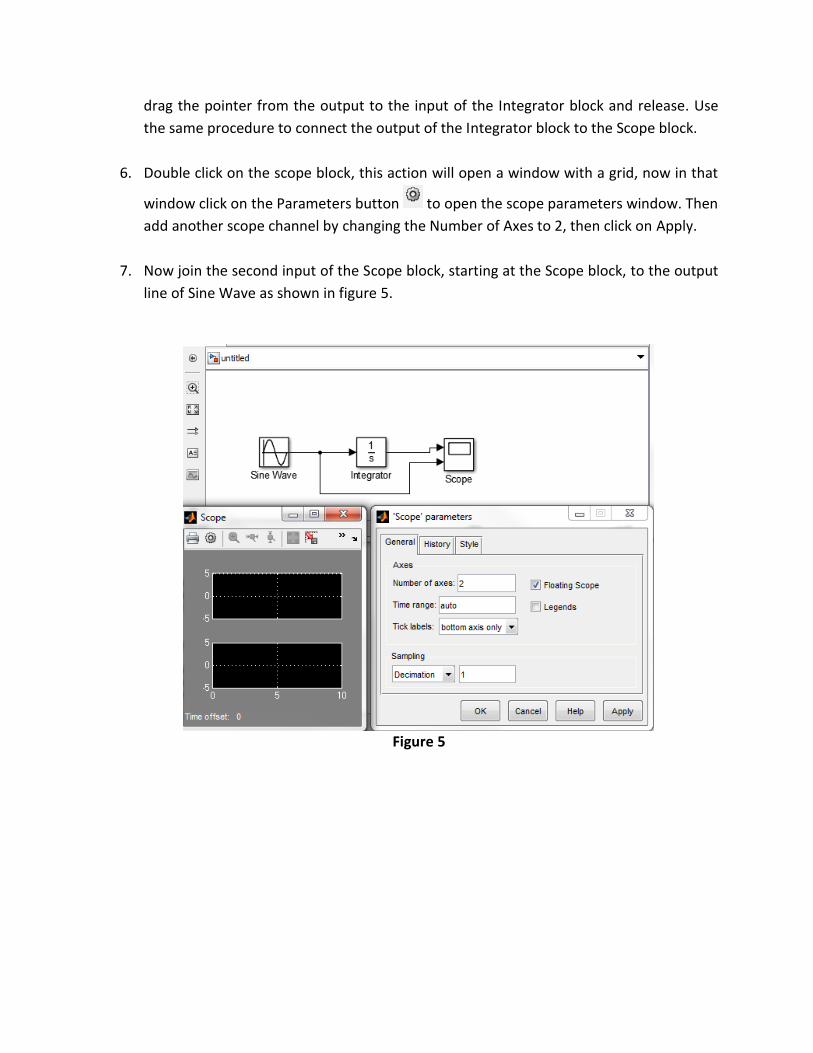
6. Double click on the scope block, this action will open a window with a grid, now in that

window click on the Parameters button to open the scope parameters window. Then

add another scope channel by changing the Number of Axes to 2, then click on Apply.

7. Now join the second input of the Scope block, starting at the Scope block, to the output

line of Sine Wave as shown in figure 5.

Figure 5

8. Be sure the Scope window is still open then click on the start simulation button in

the model window. Once clicked the model is simulated and the output response can be

viewed in the Scope window, as shown in the figure 6.

Figure 6

9. Simulate the above model by replacing the sine wave by a Pulse Generator and verify if

the response obtained is as shown in figure 7, use the zoom tools.

Figure 7

10. To view the zoomed output and to determine the exact response Right click on the

graph and then click on “Auto scale” or or left click on the mouse and then select

the region for which you need the exact response.

11. The start time and the stop time of the simulation can be altered to the desired values

by clicking on simulation tab in the model window, then and click on Configuration

parameters that will open the Configuration parameters window. In this window along

with the start time and the stop time many other options are available to customize the

model simulations

12. Save your Model, then close and reopen the model by typing its name in the MATLAB

command window.

Modeling Mathematical Equations using Simulink:

Next you will use Simulink to model the function y(t);

y(t) A cos( t )

where :

A amplitude

angular frequency

t time

phase

Define: A 2

5 Rad/s

1. Open the new model window from the File menu of Simulink library browser.

2. Choose Sources in Simulink library browser and then add two Constant blocks to your

model to be used for Phase and Frequency in the model window.

3. Next add a Ramp block to your model window. This will be used as a time source

4. Choose Math operations in Simulink library browser and then add ;

i. Product block to multiply Frequency and Time

ii. Sum block to add( t )

iii. Trigonometric function block

iv. Gain block for amplitude

5. Choose sinks in Simulink library browser and then add a scope to your model.

6. Now join the outputs and inputs of each block as shown in the figure 8. Double click on

each block to enter the correct values, figure 8. Then click on the simulate block to

simulate the model. Double click on scope to see the output. Change some parameters

and view the results.

Figure 8

Other applications Round/ceil/floor: These functions round the value of the output to the nearest decimal place.

Let’s now try and simulate the above functions for a sine wave

1. Open and assemble a new model as shown in figure 9

2. Simulate the model and print your output

3. Try this: make 2 inputs on the scope and check one output without rounding the result.

. Figure 9

Transformations Using Simulink various parameters can be converted from one type of unit to the other and the

output can be viewed conveniently.

1. Open a new Simulink model window and assemble as shown in figure 10. Hint Simulink

Extras for the conversion block

2. Simulate for different values of temperature (22F, 32F, 212F) and print the output.

Figure 10

Exercise As a first approximation, sound waves can be described using rays to express position, propagation direction, and propagation path. An equation describing echo can be defined as;

1

k

k

p

k k

k

where :

x(n) represents the straight path signal

a is an attenuation factor between 0 and 1 for reflected signals

d is a time delay for reflected sig

y(n) x(n) a x(n d )

nals

In this equation y(n) is the sound sink and the straight path ray from the sound source is represented by x(n). The summation represents any reflected rays that make it to the sink. The summation takes into account the energy loss due to reflection ak and the increase in time, or delay dk, taken to reach the sink. The scenario for three rays is shown in the figure 11. Here the source is the speaker and the sink is the microphone.

Figure 11

1. Using the echo equation, write an expression that represents figure 11.

2. Using Simulink build a model for your expression derived in step 1. For the source use

the block labeled “From multimedia File” located in the DSP Toolbox/Sources. For the

sink use the block labeled “To Audio Device” located in the DSP Toolbox/Sinks. This will

allow you to load a .wav file for the sound, and play the output to the computer

speakers. Use a Delay block from DSP Toolbox/Signal Operations for signal delays, use

SUM blocks, circles, for adding

3. Vary the values of attenuation and delays while observing the changes in the output.

Microphone Speaker

Straight Path Ray

Ray 1

Ray 2