preliminary evaluation of a mobile platform for the non

Preliminary Evaluation of a Mobile Platform for the

Non-Invasive Screening and Prevention of Diabetes

by

Kwabena Ofori-Atta

Submitted to the Department of Electrical Engineering and Computer Science

in partial fulfillment of the requirements for the degree of

Master of Engineering in Computer Science and Molecular Biology

at the

MASSACHUSETTS INSTITUTE OF TECHNOLOGY

May 2020

© Massachusetts Institute of Technology 2020. All rights reserved.

Author . . . . . . . . . . . . . . . . . . . . . . . . . . . . . . . . . . . . . . . . . . . . . . . . . . . . . . . . . . . . .

Department of Electrical Engineering and Computer Science

May 18, 2020

Certified by . . . . . . . . . . . . . . . . . . . . . . . . . . . . . . . . . . . . . . . . . . . . . . . . . . . . . . . . .

Richard R. Fletcher

Research Scientist, D-Lab

Thesis Supervisor

Accepted by . . . . . . . . . . . . . . . . . . . . . . . . . . . . . . . . . . . . . . . . . . . . . . . . . . . . . . . .

Katrina LaCurts

Chair, Master of Engineering Thesis Committee

3

Preliminary Evaluation of a Mobile Platform for the

Non-Invasive Screening and Prevention of Diabetes

by

Kwabena Ofori-Atta

Submitted to the Department of Electrical Engineering and Computer Science on

May 18, 2020, in partial fulfillment of the

requirements for the degree of

Master of Engineering in Computer Science and Molecular Biology

Abstract

Diabetes mellitus is a global health complication that has become increasingly prevalent. With

millions of individuals developing diabetic symptoms, and a similar number of individuals dying

to the disease, it is imperative that doctors and researchers develop tools that aid in diabetes

treatment and prevention to deminish the load on various global healthcare systems. Despite

advancements in treatment technologies, many of the current tools for diabetes screening are too

expensive, too prone in causing infection, or not logistically practical for use in a majority of

developing nations.

This thesis presents a deep exploration of diabetes pathogenesis and etiology, as well as

preliminary analyses of current and emerging non-invasive technologies for diabetes detection.

Evaluation methods include an image quality analysis for patient image data, a diabetes

questionnaire analysis, and the production of a semi-supervised autoencoder for patient labeling.

The exploration of diabetes pathogenesis and etiology revealed that diabetes development

can be broken down into six stages: Healthy (Stage 0), Compensation (Stage 1), Stable

Adaptation (Stage 2), Unstable Early Decomposition (Stage 3), Stable Decomposition (Stage 4),

and Severe Decomposition (Stage 5). With this biological understanding, this thesis reviews

current and emerging non-invasive technologies for diabetes screening—including infrared

thermal imaging, skin fluorescence spectroscopy, retinal and iris imaging, nail fold

capillaroscopy, pulse wave analysis, and breath analysis. The Mobile Technology Group, within

the MIT D-Lab, has designed a mobile platform that integrates several of these non-invasive

tests for diabetes—including clinical questionnaires, thermal imaging, iris imaging, retina

imaging, and finger photoplethysmography (PPG)—that can be used to predict the severity of a

patient’s diabetic condition. These technologies are part of a clinical field study that is currently

ongoing in Mumbai and Bangalore, India. This thesis presents two image data quality metrics—

blur and saturation detection—that were developed and implemented to automatically assess the

quality of image data collected in the field. The results of the analysis showed that blur detection

4

via fast Fourier transform (FFT) and via Laplacian kernel are both effective methods, with the

FFT method providing a tunable and more gradual measure of blur.

The preliminary analyses of the India study data focused on the Diabetes Questionnaire.

Since most study subjects were undergoing a form of treatment for diabetes, little correlation was

found between patient diabetic indicators—as measured by the Indian Diabetes Risk Score

(IDRS)—and patient random blood sugar (RBS) measurements. However, there is moderate

correlation between patient RBS values and IDRS values among un-medicated patients,

indicating that risk score can be used as a proxy for diabetes severity. Having used the IDRS

values to create ground truths for patient labeling, a semi-supervised autoencoder was developed

to enable scalable labeling of patient data. The autoencoder performed reasonably well, having a

class-average area under the receiver operator characteristic (AUROC) of 0.845, and a class-

average area under the precision-recall (AUPR) curve of 0.789. However, clustering methods

using dimensionality reduced patient features (derived via autoencoder, PCA, and t-SNE) were

less effective, yet the autoencoder still outperformed the controls. Since data collection is on-

going, the predictive power of the autoencoder and its dimensionality reduction functionality is

likely to improve with the addition of more patients and more measurements (i.e. retina, iris, and

thermal image scores, PPG scores, and other questionnaire data).

Thesis Supervisor: Richard R. Fletcher

Title: Research Scientist, D-Lab

6

Acknowledgements

I would first like to acknowledge my advisor, Richard Fletcher. Throughout this research

process, Dr. Fletcher has consistently guided and challenged me, pushing my work to new

heights. He is incredibly dedicated to his work, and his drive to improve global health outcomes

through innovative technologies is truly inspiring. From the Mobile Technology Group, I would

like to thank Saadiyah Husnoo for her technical guidance and direct contributions to the project.

I would also like to thank Bernardo García Bulle Bueno and Ellie Simonson for their helpful

advice throughout my research process. I would also like to acknowledge our wonderful partners

in India at S-VYASA and AJFTLE.

Finally, I would like to thank my family and friends who have shown me nothing but

unconditional love, guidance, and support throughout this entire process. I could not have not

made it to this point without them.

8

Contents

1. Introduction and Motivation ..........................................................................................15

1.1 Global Health Crisis ...............................................................................................15

1.2 The Importance of Screening Tools .......................................................................16

1.3 The Benefits of Non-Invasive Screening Tools .....................................................16

1.4 Current Work in Non-Invasive Diabetes Diagnostics ...........................................17

1.5 Scope of Thesis ......................................................................................................17

2. The Time Evolution of Diabetes and Cardiometabolic Syndrome ..............................20

2.1 Stage One: Compensation ......................................................................................21

2.1.1 Description .................................................................................................21

2.1.2 Symptoms ..................................................................................................21

2.1.3 Risk Factors ...............................................................................................22

2.1.4 Diagnostic Tests .........................................................................................23

2.1.5 Concurrent Diseases...................................................................................24

2.2 Stage Two: Stable Adaptation ...............................................................................25

2.2.1 Description .................................................................................................25

2.2.2 Symptoms ..................................................................................................26

2.2.3 Risk Factors ...............................................................................................26



2.3 Stage Three: Unstable Early Decomposition .........................................................27

2.3.1 Description .................................................................................................27

2.3.2 Symptoms ..................................................................................................28

2.3.3 Risk Factors ...............................................................................................28


9


2.4 Stage Four: Stable Decomposition.........................................................................30

2.4.1 Description .................................................................................................30

2.4.2 Symptoms ..................................................................................................30

2.4.3 Risk Factors ...............................................................................................31



2.5 Stage Five: Severe Decomposition ........................................................................31

2.5.1 Description .................................................................................................31

2.5.2 Symptoms ..................................................................................................32

2.5.3 Risk Factors ...............................................................................................33



2.6 The Effects of Diabetes Medications .....................................................................34

2.6.1 Metformin ..................................................................................................35

2.6.2 Sulfonylureas and Meglitinides .................................................................35

2.6.3 Thiazolidinediones .....................................................................................36

2.6.4 Insulin ........................................................................................................36

2.7 Discussion ..............................................................................................................36

3. Emerging Technologies and Tools for Non-Invasive Diabetes Detection ...................39

3.1 Infrared Thermal Imaging ......................................................................................39

3.2 Skin Fluorescence Spectroscopy............................................................................41

3.3 Retina and Iris Imaging ..........................................................................................42

3.4 Nail Fold Capillaroscopy .......................................................................................44

3.5 Pulse Wave Analysis..............................................................................................47

3.6 Breath Analysis ......................................................................................................49

4. Implementation of Non-Invasive Diabetes Screening Tools and Clinical Study........52

4.1 Study Design and Protocol.....................................................................................53

4.2 Available Data and Current Status .........................................................................55

5. Image Quality Analysis for Patient Image Data ...........................................................57

10

5.1 Automated Detection or Blur .................................................................................58

5.1.1 Fast Fourier Transform (FFT) Blur Metric ................................................58

5.1.2 Laplace Operator Blur Metric ....................................................................59

5.1.3 Comparing and Contrasting Metrics ..........................................................60

5.2 Automated Detection of Saturation .......................................................................64

6. Diabetes Questionnaire Analysis ....................................................................................68

6.1 Data Preprocessing.................................................................................................68

6.2 Heatmap Correlation Analysis ...............................................................................73

7. Semi-Supervised Autoencoder for Patient Labeling ....................................................80

7.1 Motivation Behind the Semi-Supervised Autoencoder and Initial Assumptions ..80

7.2 Methods..................................................................................................................81

7.2.1 Autoencoder Input Features .......................................................................81

7.2.2 Ground Truth Label Formation ..................................................................82

7.2.3 Autoencoder Hyperparameters and Architecture.......................................83

7.2.4 Dimensionality Reduction Analysis ..........................................................85

7.3 Results ....................................................................................................................86

7.3.1 Patient Labeling via Autoencoder ..............................................................86

7.3.2 Dimensionality Reduction via Autoencoder ..............................................86

7.4 Discussion ..............................................................................................................91

8. Conclusion and Future Work .........................................................................................94

8.1 Contributions of Work ...........................................................................................94

8.1.1 Exploration into the Biological Characteristics of Diabetes and Non-

Invasive Technologies to Detect Them......................................................94

8.1.2 Image Quality Metrics for the Improvement of Image-Based Predictive

Models........................................................................................................94

8.1.3 Preliminary Semi-Supervised Autoencoder for Patient Labeling ..............94

8.2 Future Work ...........................................................................................................95

8.3 Larger Impact .........................................................................................................96

11

List of Figures

2-1 The complete time evolution of diabetes (stage 1 through stage 5) and its adjacent

disorders and complications ...................................................................................34

3-1 Example infrared thermal image of the face ..........................................................40

3-2 Application of various skin fluorescence spectroscopy devices in practice ..........42

3-3 Iridology chart for both the right and left irises .....................................................44

3-4 Example of capillaroscopic alterations in a diabetic patient and a healthy subject

................................................................................................................................46

3-5 Pulse waveform schematic depicting the measured and calculated values during

pulse wave analysis ................................................................................................48

4-1 Diagram of the system architecture developed by the Mobile Technology Group

for clinical study field work regarding the evaluation of non-invasive diabetes

screening tools .......................................................................................................52

4-2 Sample screenshots of mobile applications developed by The Mobile Technology

Group to support field testing of diabetes screening tools .....................................53

5-1 Examples of patient thermal, retina, and iris images (displayed left to right) .......58

5-2 2D Laplacian kernel ...............................................................................................59

5-3 Blur metric comparison using fully gaussian-blurred images with incrementally

increasing blur strength ..........................................................................................61

5-4 Blur metric comparison using partially gaussian-blurred images with an

incrementally increasing number of blurred quadrants .........................................62

5-5 Blur metric comparison using partially gaussian-blurred images that were

gradually blurred to a fully blurred image .............................................................63

5-6 Saturation metric applied to an iris image at varied saturation levels ...................65

5-7 Saturation metric and situational corrections applied to a retina image ................66

6-1 Heatmap analysis of 29 patient features across 174 patients .................................74

12

6-2 Heatmap analysis of 29 patient features across 24 patients who have not

undergone any diabetes treatments ........................................................................76

6-3 Scatterplot depicting the correlation between RBS and IDRS among the 24

untreated patients in the 174-patient population ....................................................77

7-1 Semi-supervised autoencoder architecture ............................................................84

7-2 Division of 212 patients into training and testing datasets via 50/50 split ............85

7-3 Receiver operating characteristic (ROC) curves of the binarized multi-class

predictions of the semi-supervised autoencoder ....................................................87

7-4 Precision-recall curves of the binarized multi-class predictions of the semi-

supervised autoencoder ..........................................................................................88

7-5 Dimensionality reduction of 106 patient feature vectors via autoencoder ............89

7-6 Dimensionality reduction of 106 patient feature vectors via controls (PCA and t-

SNE) .......................................................................................................................90

13

List of Tables

6-1 Numerical conversions applied to the Diabetes Questionnaire patient data ..........69

6-2 Numerical conversions applied to features derives from Diabetes Questionnaire

patient data .............................................................................................................73

6-3 Pearson and Spearman correlation coefficients for the correlation between RBS

and IDRS among the 24 untreated patients in the 174-patient population ............78

7-1 Average silhouette coefficients of the ground truth clusters within the original

dataset and the various dimension-reduced patient representations ......................91

15

Chapter 1

Introduction and Motivation

The world, as a global community, is continuously striving for innovation and groundbreaking

research in the medical and life sciences—numerous studies within the fields of biomedical

engineering, pharmacology, systems biology, etc. have been published to display these feats of

human ingenuity. Yet despite these revolutionary discoveries, many individuals around the world

remain desperately in need of healthcare to combat various common, curable, and preventable

conditions.

1.1 Global Health Crisis

There are numerous causes for this innovation-healthcare disparity, but many of these

contributors ultimately boil down to two factors: the availability of healthcare workers, and the

cost of treatment. Firstly, many people don’t have access to healthcare. The World Health

Organization (WHO) has stated that approximately half of the world’s 7.3 billion people cannot

access essential health services[1]. This is mainly due to the overwhelming number of people who

are in need of medical assistance with respect to the number of active and accessible physicians.

About 40% of countries have fewer than 10 doctors for every 10,000 individuals[1]. The world is

estimated to have a shortage of 18 million healthcare professionals by 2030 (mainly in lower-

income countries)[1].

Secondly, the cost of healthcare is becoming increasingly unmanageable for both citizens

and governmental bodies. In 2010, over 800 million people worldwide spent at least 10% of their

household budget on healthcare, and nearly 100 million people worldwide fell below the poverty

line as a result of their healthcare spending[1]. On a larger scale, the United States spent over

$10,000 on healthcare per capita in 2017 (the most of any other country), with 20 other countries

16

spending over $3,000 per capita the same year[2]. With these high healthcare costs, it’s incredibly

difficult for countries to manage a standard quality of healthcare for everyone, and this burden is

especially felt in rural and developing nations.

1.2 The Importance of Screening Tools

In order to combat the complications of traditional healthcare, more widespread, cost-effective

methods of disease screening are emerging. These screening methods tend to be non-invasive

measurements and visualization that are often more readily accessible than physicians. These

diagnostic tools allow individuals to obtain a preliminary metric that informs them of their

potential disease state, as well as whether or not to seek further medical assistance/care. If used

appropriately, these screening tools can help individuals in need seek medical assistance in a

timely manner, or even instruct individuals on how to prevent certain medical conditions from

even occurring. Most importantly, it will allow physicians to tend to patients whom are at high

risk levels (rather than need to examine every potential patient)—ultimately this would decrease

the intense burdens on various global healthcare systems.

1.3 The Benefits of Non-Invasive Screening Tools

While massively scaled screening tools are useful for identifying which individuals are in need

of treatment and targeted health education, there are many practical reasons that inhibit the

widespread use of screening tools. For tests that traditionally require biological specimens—such

as blood, urine, or sputum—these specimens must be collected, labelled, and transported to a

laboratory facility at another location. In addition, systems for recoding and tracking patient

medical records are needed in order to ensure that each patient receives their results.

Furthermore, due to poor supply chains, tests and materials are often in short supply or out of

stock. Since stable health infrastructure are lacking in many low-resource regions around the

world, screening tests that require biological specimens have presented a great challenge for

public health.

As an alternative, new technologies are emerging that enable other methods of

diagnosing certain health conditions non-invasively. While most of these methods do not possess

the sensitivity and specificity of a biochemical laboratory test, these new methods enable simpler

17

and scalable screening for disease. In general, non-invasive tests are faster to perform, give

immediate results, and don’t require any consumable supplies or materials. These technologies

thus represent a significant step forward in the surveillance and management of disease.

1.4 Current Work in Non-Invasive Diabetes Diagnostics

Much work has been done to explore non-invasive diagnostic systems for diabetes due to its

global prevalence. Diabetes affects people around the world, with the number of diseased

individuals rising more rapidly in low- and middle-income countries. According to the WHO,

diabetes was the direct cause of 1.6 million deaths each year, and the global prevalence of

diabetes in adults has risen from 4.7% in 1980 to 8.5% in 2014[3]. As the number of diseased

individuals increases, so will the global cost of diabetes-related medical care. By 2030, the

global cost of diabetes is projected to rise to an all-time maximum of 2.2% of global GDP[4].

The Mobile Technology Group, headed by Dr. Fletcher, has developed numerous low-

cost, non-invasive tools to improve clinical decisions around various global diseases—some

tools include peak flow meters for detecting pulmonary disorders, mobile games to monitor

mental health, and imaging algorithms to screen for infectious diseases[5]. One of the most

significant ventures that the Mobile Technology Group has made in the field of diabetes research

is their development of a mobile application which allows individuals to screen themselves for

diabetes severity. Even though the application is still in development, there have been great

strides for producing predictive models using non-invasive measurements that are cost-effective

and accessible for a majority people around the world[5][6].

1.5 Scope of Thesis

The content of this thesis is focused on exploring the intricacies of diabetes and non-invasive

diagnostic/screening tools for diabetes. This thesis will also address in-depth analyses of patient

data (collected by clinicians for the use of predictive model training), and methods of

cleaning/preparing patient data—presented analyses and methodologies are intended to improve

model training and overall predictive power of machine learning algorithms associated with the

Mobile Technology Group’s diabetes screening mobile application. Chapter 2 of this thesis

explains the time-based pathology and etiology of diabetes and other concurrent disorders. In

18

Chapter 3, various emerging and common non-invasive metrics for diabetes screening are

presented and analyzed for their efficacy. Chapter 4 describes the study design and protocol for

the mobile application as well as its current status. Chapter 5 explores metrics to assure quality

control of patient image data. In Chapter 6, patient data from the Mobile Technology Group’s

Diabetes Questionnaire is assessed for its correlation to patient blood sugar levels (a common

metric for diabetes screening). Chapter 7 discusses the use of a semi-supervised autoencoder for

the diabetic severity labeling of patient data. Chapter 8 discusses conclusions derived from the

all analyses, and future work aimed to improve the current mobile application for diabetes

screening.

20

Chapter 2

The Time Evolution of Diabetes and Cardiometabolic

Syndrome

Within the past decade, a significant rise in chronic diseases—such as diabetes, hypertension,

and obesity—has been observed in both industrialized and developing nations alike. With the

influx of these maladies, there is also a concurrent influx of cardiometabolic syndrome (CMS),

which is the umbrella condition that includes all these diseases[7]. CMS is a combination of

multifactorial diseases spanning maladaptive cardiovascular, renal, metabolic, prothrombotic,

and inflammatory abnormalities and dysfunctions[8]. The syndrome is mainly characterized by

insulin resistance, impaired glucose tolerance, dyslipidemia, high blood pressure, non-alcoholic

fatty liver disease, and central adiposity[9][10]. The condition of CMS continues to advance as a

threatening disease, and it has already been recognized as an entity by the World Health

Organization and the American Society of Endocrinology[9]. In order to combat the diffusion of

the disease, it is imperative to understand how CMS manifests, and the many factors which

influence its intensity.

One of the most common diseases associated with CMS and its complications is diabetes.

Diabetes was the seventh leading cause of death in the United States in 2017, and 1.5 million

Americans are diagnosed with diabetes every year[11][12]. Despite being a well-known and

researched disease, diabetes is often studied as an isolated illness. Diabetes progression develops

concurrently with numerous other biological conditions all under the CMS umbrella; the

etiologies of each of these unique conditions are intertwined. Revealing the time-varying

connections between diabetes and other cardiometabolic conditions may unveil new methods of

preventing and treating diabetes, concurrent diseases, and CMS as a whole.

21

Diabetes is strongly linked to the body’s management of insulin and blood sugar levels.

This regulation is completed via the islets of Langerhans within the pancreas. The most relevant

portion of the pancreatic islets, related to the development of diabetes, is the beta cell mass. The

beta cells are responsible for secreting insulin into the circulatory system after sensing an

increase of glucose[13]. The onset of diabetes is closely linked to abnormalities within the

function of beta cells, and the severity of diabetes grows with the decline of beta cell function.

Due to this, diabetes severity can be tracked by the presence or absence of specific metabolic

processes. There are five major stages within diabetes pathogenesis, with stage zero being a

healthy individual.

2.1 Stage One: Compensation

2.1.1 Description

The onset of diabetes actually begins with a slightly different precursor disease known as

prediabetes—this condition accounts for the first three stages of diabetes. Stage one is known as

Compensation[14]. During this stage, an individual will move from a healthy state, to one where

insulin resistance begins to manifest.

Due to the manifestation of insulin resistance, the beta cells within the pancreas will

increase the amount of insulin released in response to blood glucose, causing a spike in acute

insulin response (AIR)[14]. This is done by increasing the number of beta cells and/or the size of

each beta cell in the pancreas[14][15]. The increase in AIR reflects the compensatory measure the

body takes in order to counteract insulin resistance during the Compensation stage; the increase

in insulin is generally able to maintain normal blood glucose levels despite the developing

resistance. As a result of these metabolic processes, numerous symptoms may occur. For

instance, the beta cells may overcompensate when releasing increased levels of insulin, causing

blood glucose to deplete and inducing hypoglycemia—usually occurring 2-3 hours after a meal

when beta cells are most active[16].

2.1.2 Symptoms

With respect to beta cell insulin production, the increased levels of insulin in the Compensation

stage may induce hyperinsulinemia as well, driving an individual to exhibit symptoms of both

22

hyperinsulinemia and prediabetes. The following conditions are symptoms of hyperinsulinemia:

weight gain, strong cravings for sugar, intense feelings of hunger or frequent feelings of hungry,

anxiety, a lack of concentration/motivation, and fatigue[17]. Some of these symptoms—such as

weight gain, cravings for sugar, and intense and/or frequent hunger—are directly linked to

eating. High insulin levels would lead to low blood sugar levels, resulting in a need to increase

blood sugar levels via dietary consumption. Similarly, other symptoms like anxiety, a lack of

concentration/motivation, and fatigue are linked to energy storage and energy depletion. Since

blood sugar levels would be too low to supply sufficient energy, various tissues in the body

wouldn’t receive enough nutrients to operate naturally and efficiently. Regardless, the presence

of these symptoms generally go unseen, and many symptoms are difficult to connect solely to

prediabetes given their prevalence in various other ailments.

2.1.3 Risk Factors

Insulin resistance may result from various factors. Individuals can be predisposed to resistance

through genetics, or certain lifestyle behaviors can influence the induction of the condition. It has

been postulated that free fatty acid metabolites, created from breaking down fatty acids, can

interfere with downstream insulin signaling[18]. Likewise, the dysfunction of certain surface

protein complexes, or the phosphorylation of specific intracellular proteins, may hinder insulin

signal transduction or lead to reduced insulin receptor expression[18]. Even mitochondrial

dysfunction may contribute to insulin resistance, triggering the activation of several serine

kinases and weakening insulin signal transduction[18].

It is likely that one of the most common triggers for developing insulin resistance in

diabetes—outside of genetics—is a result of free fatty acid metabolites. This conclusion ties the

manifestation of prediabetes to its risk factors. The risk factors of the Compensation stage of

prediabetes are the following: a family history of diabetes, an increase BMI, a waist size greater

that 40 inches (men) or 35 inches (women), an age of 45 years and older, ethnic minorities

(African-American, Hispanic, Native American, Asian American, Pacific Islander), a history of

smoking, general inactivity, sleeping problems or sleep disorders, increased triglyceride levels,

decreased HDL-cholesterol levels, high blood pressure (hypertension), and a history of one or

more vascular diseases[19]. From this list, it’s clear that some of the most common risk factors for

developing prediabetes are habits and conditions which increase the number of free fatty acids in

23

the body—the other factors being genetic, resulting in a genetic cause of insulin resistance

manifestation in those cases.

At times in which the body has excess amounts of blood glucose—possibly due to a large

meal with minimal energy consumption following—the sugar is rarely dispelled from the body.

As a precious source of energy, unused glucose is stored in the body, often being converted into

glycogen, triglycerides, and also free fatty acids by the liver. When this energy source must be

used (i.e. in times of starvation), these macromolecules are broken down by various metabolic

processes to catalyze reactions, ultimately creating the metabolites. The abundance of the free

fatty acid metabolites are part of what block insulin signaling, initiating the Compensation stage.

2.1.4 Diagnostic Tests

Since blood glucose levels do not chance in the Compensation stage, and direct symptoms are

difficult to perceive for prediabetes, there are no formal tests to determine if an individual is in

this stage. Nevertheless, the Compensation stage is marked by an increase in insulin

(hyperinsulinemia) that can be measured via simple blood tests. Having plasma insulin levels

higher than 2 µU/mL, as well as a serum glucose concentration that is less than 60 mg/dL, is

indicative of having hyperinsulinemia[20]. Nevertheless, clearly defined and elevated insulin

levels are not always present in a state of hyperinsulinemia, especially at the time of

hypoglycemia. Therefore, the detection of suppressed beta-hydroxybutyrate (less than 1 µmol/L)

in conjunction with low levels of free fatty acids (less than 1 µmol/L) during a period of

hypoglycemia may also be necessary to indicate hyperinsulinemia[20]—however, these

alternative conditions are less likely to be observed in prediabetes specifically due to the strong

contribution that free fatty acids metabolites have in the manifestation of diabetes.

Throughout the manifestation of prediabetes, individuals may develop cardiovascular

diseases (CVD) as well. Most of these concurrently developing diseases involve complications in

blood vessel integrity. These conditions can therefore be monitored using CVD diagnostic tests.

The progression and severity of CVD is linked to the progression and severity of diabetes, so it’s

beneficial to accompany diabetes diagnostic tests with measures marking CVD progression—

some CVD diagnostic tests already used for analyzing diabetic states are infrared/thermal

imaging and skin fluorescence spectroscopy[21][22].

24

2.1.5 Concurrent Diseases

Prior to the Compensation stage, inflammation may develop in and around the adipose tissues of

the body[23]. As adipose cells grows in mass, they recruits more immune cells within their

tissues[24]. Both the adipose and immune cells synthesize and secrete proinflammatory

adipokines, cytokines, and chemokines which produce the aforementioned inflammation[23].

These proinflammatory compounds activate cellular pathways which lead to insulin resistance—

this means that inflammation is highly correlated to abnormal insulin signaling[25]. The insulin

resistance will then result in producing higher levels of blood glucose to be turned into fat,

growing adipose tissue mass and producing even more inflammation[23][24]. This inflammation

response is strongly related to the risk factors of the Compensation stage given that adipose

tissue grows in mass with increased triglycerides levels; therefore, inflammation can precede

prediabetes or both conditions can develop simultaneously.

To further support this claim, studies have shown that in conditions of hyperinsulinemia,

individuals may show early signs of atherosclerosis—however, atherosclerosis is not guaranteed

to manifest during this stage of diabetes[26]. Atherosclerosis is one of the major vascular diseases

triggered by prediabetes, and it is characterized by the hardening of arteries due to plaque

buildup within the arterial walls—these plaques being composed of fat, cholesterol, calcium, and

other substances within the blood[27]. In a homeostatic environment, insulin is involved in the

activation of endothelial nitric oxide synthase (eNOS) which subsequently produces nitric

oxide[26]; NO dilates the blood vessels, relaxing them and allowing for improved blood

flow[26][28]. Ultimately, this process prevents atherosclerosis by preventing the arterial walls from

thickening. However, hyperinsulinemia promotes the down-regulation of the Akt/PKB signaling

pathway within endothelial cells by overstimulating the insulin receptors, leading to insulin

resistance. This leads to less eNOS activation and nitric oxide production, promoting the

hardening of blood vessel tissue and the initiation of atherosclerosis[26].

Since atherosclerosis can affect any artery in the body, there are various related diseases

that may develop from this condition, such as the following: ischemic heart disease (coronary

heart disease/coronary artery disease), carotid artery disease, peripheral artery disease, and

chronic kidney disease[27]. Likewise, a complete blockage of an artery, due to atherosclerosis

plaque buildup, could result in a heart attack or stroke[27]. Once atherosclerosis develops, all

subsequent vascular diseases are no longer directly influenced by specific stages of diabetes, and

25

therefore cardiovascular pathogenesis begins to proceed separately. Nevertheless, the increased

severity of diabetic symptoms proportionally increases one’s risk of developing vascular damage

and/or CVD—as well as the rate at which current cardiovascular complications advance—as will

be described in the future stages of diabetes.

Insulin resistance will continue to develop if there is no intervention during the

Compensation stage. Once insulin resistance grows to a point where beta cells function can no

longer fully compensate, the prediabetes disease progresses to stage two: Stable Adaptation[14].

2.2 Stage Two: Stable Adaptation

2.2.1 Description

The Stable Adaptation stage is marked most notably by a gradual increase in blood glucose

above a normal level. This stage is also marked by a slight decrease in AIR. The decline in

insulin production/secretion can arise from various causes that can be linked to genetic and

environmental forces. In some cases, the immune system reacts to the influx of insulin being

produced by the beta cells. The immune system then attacks the beta cells, slowly destroying

them and inducing type 1 diabetes[29]. Over time, beta cell mass will deplete and the body will be

unable to naturally produced sufficient levels of insulin, making the individual completely

dependent on an outside source of insulin; however, this would take place in latter stages of the

disease. The autoimmune response against the beta cells may be related to the body’s

autoimmune response against cancerous cells—cancerous beta cells can produce insulin in

chaotic and abundant quantities, similar to how beta cells in stage one behave. Destroying the

beta cells would decrease the amount of insulin being produced, and therefore diminish the AIR.

Similarly, decreasing insulin production would increase blood glucose. Nevertheless, the Stable

Adaptation stage is not always triggered by an autoimmune response.

Beta cells may become less responsive to high levels of blood glucose[30]—similar to how

the various cells of the body become less responsive to insulin throughout stage one and two.

Due to this glucose resistance, the beta cells would not produce as strong of a glucose-stimulated

insulin response, leading to less insulin secretion. Progression of this decrease in beta cell

activity will lead to type 2 diabetes. Over time, the body will stop producing healthy amounts of

insulin, but the individual will not be completely dependent on an outside source of insulin.

Depending on the method of beta cell decline, the Stable Adaptation stage can be fairly brief or

26

last a lifetime. This stage of prediabetes remains stable as long as insulin production prevents

sharp rises in blood glucose.

2.2.2 Symptoms

The main symptoms of the Stable Adaptation stage are the increase in blood glucose and the

decrease in AIR mentioned previously. Depending on the extent of which insulin production has

decreased, one may still experience symptoms of symptoms the Compensation stage of

prediabetes, including hyperinsulinemia. As blood glucose increases and insulin production

decreases, these symptoms should subside—if they are present—and symptoms of

hyperglycemia may begin to appear. These symptoms include the following: increased thirst

and/or hunger, frequent urination, sugar in the urine, headache, blurred vision, and fatigue[31].

Nevertheless, the strength of these symptoms should be weak within this stage. The symptoms of

hyperglycemia and hyperinsulinemia (symptoms from the Compensation stage) are somewhat

similar, mainly because both are related to dysglycemia—abnormal blood glucose.

2.2.3 Risk Factors

Given that the Stable Adaptation stage is a stage within prediabetes, the same risk factors

mentioned in stage one will apply as risk factors for this stage too. The only additional risk factor

would be the presence of symptoms related to hyperinsulinemia, given that hyperinsulinemia

was a symptom of the prior stage.


Since the blood glucose level increases past the normal range during this stage, there are various

tests to measure glucose metabolism in order to check whether one is in this stage of prediabetes.

However, normal blood glucose can be defined in a variety of ways, especially since glucose

levels can vary significantly within short periods of time due merely to the nature of the various

metabolic processes taking place. Nevertheless, there are three major methods of measuring

blood glucose levels which are effective when diagnosing stages of diabetes: average blood

glucose via the A1C test, fasting plasma glucose (FPG) via the FPG test, and two-hour postload

glucose via an oral glucose tolerance test (OGTT)[32]. The A1C test measures average blood

glucose levels over 2-3 months by analyzing the percentage of glycated hemoglobin in

27

circulation over that time period. The FPG test measures the concentration of glucose in the

blood after an eight-hour period of avoiding food. Lastly, the OGTT examines the concentration

of blood sugar remaining in the blood over a two-hour period, after ingesting 75g of sugar orally.

Each test can be used to establish a healthy baseline, as well as track how one progresses through

the stages of diabetes.

In stage one, an individual maintains normal glucose levels, meaning an A1C of less than

5.7%, a FPG of less than 5.6 mmol/L (100 mg/dL), and an OGTT of less than 7.8 mmol/L (140

mg/dL)[32]. However, in stage two, blood glucose levels rise to slightly abnormal levels: A1C of

approximately 5.7%, FPG of approximately 5.6 mmol/L (ranging between 5.0 and 6.1 mmol/L

(89–110 mg/dL))[14][33], and OGTT of around 7.8 mmol/L[32].


In this stage, it is unlikely that any new conditions manifest, especially since the prediabetic

stages do not exhibit strong symptoms. Nevertheless, the inflammation which manifested

during/prior to stage one may spread to more areas of the body throughout the Stable Adaptation

stage. Also, dysglycemia may worsen any cardiovascular diseases obtained up to this point—

high concentrations of sugar and/or insulin can damage blood vessels[26][35]. These conditions

develop further as individuals approach stage three: Unstable Early Decomposition[14].

2.3 Stage Three: Unstable Early Decomposition

2.3.1 Description

The Unstable Early Decomposition stage is the final stage of prediabetes[14]. It is most notably

marked by a sharp, rapid increase in blood glucose, and an even further decline in insulin

production. Blood glucose begins to increase uncontrollably because beta cell decline has passed

a critical point. During this stage, impaired fasting glucose (IFG) and impaired glucose tolerance

(IGT) noticeably manifest. IFG is defined as having fasting glucose which is well above a

normal level (5.6 mmol/L). IGT is related to general insulin resistance, and the body’s impaired

ability to handle increased glucose in the blood. This stage is also associated with an increased

risk of cardiovascular pathology due to how glucose affects blood vessels[33]. Given by the name,

Unstable Early Decomposition is generally an unstable, transient stage because blood glucose

28

tends to shift drastically[14]. Glucose levels could easily increase to a diabetic level, yet changes

in one’s lifestyle may reverse beta cell decline and revert the disease progression back to a

previous prediabetic stage.

2.3.2 Symptoms

Unlike the Stable Adaptation stage, the blood glucose level in the Unstable Early Decomposition

stage is well above normal. This means that symptoms of hyperglycemia are highly likely to be

experienced, especially for individuals with blood glucose levels approaching the range of

diabetic levels. These would be the same hyperglycemic symptoms mentioned in the Stable

Adaptation stage, but to a stronger degree. The presence of more long-term hyperglycemia

symptoms may also appear, including fruity-smelling breath, nausea and vomiting, shortness of

breath, dry mouth, muscular weakness, and abdominal pain[34]. However, these symptoms should

be weak, if at all present, given the transience of the stage.

2.3.3 Risk Factors

The risk factors of the Unstable Early Decomposition stage are the same risk factors of the

previous two stages of prediabetes. Nevertheless, symptoms of hyperglycemia may signal the

end of the Stable Adaptation stage, which would in turn be an indicator for disease progression

into stage three.


This stage is demarcated by an interval of blood glucose between the upper limit of normal blood

glucose levels and the lower limit of diabetic glucose levels. Nevertheless, there are different

standards for defining this interval with regards to fasting glucose. By the World Health

Organization’s (WHO) criteria, individuals in this stage would have a FPG level between 6.1

mmol/L (110 mg/dL) and 6.9 mmol/L (125 mg/dL). By the American Diabetes Association’s

(ADA) criteria, individuals in this stage would have a FPG level between 5.6 mmol/L (100

mg/dL) and 6.9 mmol/L (125 mg/dL)[33].

Besides measuring FPG, this stage can also be classified by the A1C test and OGTT. An

individual would be in this stage if A1C levels are between 5.7% and 6.4% on two separate tests.

Similarly, an individual would be in this stage if one’s postload plasma glucose is between 7.8

29

mmol/L (140 mg/dL) and 11.0 mmol/L (199 mg/dL) after a two-hour period[32]. The combination

of multiple tests would more accurately diagnose this stage, however individuals are rarely found

in this stage clinically due to its transience[14].


As mentioned before, the spike in blood glucose warrants a high possibility of developing

cardiovascular disorders during this stage. Atherosclerosis is among these cardiovascular

disorders, however its development in the Unstable Early Decomposition stage can differ from

that in the Compensation stage. Atherosclerosis is commonly triggered by oxidative stress from

reactive oxidative species (ROS), and hyperglycemia can increase ROS formation through a

multitude of mechanisms[35]. For instance, ROS can deplete nitric oxide, increasing arterial

stiffness[28]. Also, ROS can cause the oxidative modification of low density lipoprotein and also

endothelial dysfunction, thereby promoting a vascular inflammatory response[36]—this

inflammation is with respect to the arterial walls, which is separate from inflammation stimulated

by adipose tissue. This vascular inflammation is what promotes blood vessel stiffening.

Besides promoting ROS production, the presence of ambient glucose in the setting of a

hyperglycemic state can stimulate the glycosylation of free amino groups in proteins, lipids,

and/or nucleic acids within blood vessel walls and adjacent tissues. These glycosylation products

rearrange over time to form irreversible end products that accumulate in and around the arterial

walls. These advanced glycation end products (AGEs) advance atherosclerosis and tissue

damage through a variety of mechanisms[35]. Similarly, the high concentrations of glucose, as a

result of hyperglycemia, can activate protein kinase C (PKC). One of the functions of PKC is

upstream regulation of a growth factor for the extracellular matrix. Overstimulating PKC will

result in the thickening of capillary basement membranes, leading to atherosclerosis[35].

As previously mentioned, the Unstable Early Decomposition stage marks the end of the

prediabetes. Without intervention, insulin production will continue to decrease and blood glucose

will continue to increase. As the stage rapidly advances, the symptoms and associated

complications of diabetes will emerge, leading to the fourth stage of diabetes: Stable

Decomposition[14].

30

2.4 Stage Four: Stable Decomposition

2.4.1 Description

This stage marks the beginning of the diabetes disease, where symptoms commonly associated

with diabetes begin to show unambiguously[14]. Individuals in the Stable Decomposition stage

are nearing beta cell failure. Nevertheless, the beta cells are still able to produce enough insulin

to avoid ketoacidosis[14]. When not enough insulin is being produced, glucose can no longer be

taken in by the cells, and the body must rely on ketone bodies (produced from fat) for energy.

Ketoacidosis is caused when the body starts breaking down fat at a rate that is too fast[37].

An individual can remain in this stage for the rest of their lifetime because the severity of

hyperglycemia reaches a stable plateau; nevertheless, hyperglycemia still has the potential to

cause various other disorders, and its likelihood of doing so increases with time. The length of

this stage is mostly dependent on beta cell survival. In the case of type 2 diabetes, beta cells are

not in danger of being destroyed. Even though hyperglycemia decreases the glucose sensitivity

of beta cells, they will continue to produce enough insulin to prevent ketoacidosis. However,

beta cell mass may decrease very slowly over time due to apoptosis[14]. In the case of type 1

diabetes, the immune system is continuously attacking and destroying the beta cells. An

individual with type 1 diabetes could rapidly progress through stage four as their beta cell mass

depletes and insulin production halts[14].

2.4.2 Symptoms

The major symptoms of diabetes begin to appear during this stage, which include the following:

tingling, numb, or painful sensations in the hands or feet, slow healing cuts and wounds, patches

of dark skin, itchy skin/yeast infections, and symptoms of hyperglycemia (mentioned in stage

two)[38]. Some of these symptoms are related to the complications which may develop as a result

of diabetes—poor blood circulation can lead to the skin and nerve conditions that are alluded to

through these symptoms.

31

2.4.3 Risk Factors

The main risk factor of Stable Decomposition is prediabetes since prediabetes must precede

diabetes. Similarly, the risk factors of the three stages of prediabetes would also be the risk

factors of the Stable Decomposition stage.


The metric for a diabetic fasting blood glucose level is consistent with both the WHO and the

ADA. Individuals in this stage would have a FPG level of 7.0 mmol/L (126 mg/dL) or greater[32].

An individual would also be classified in this stage if they have A1C levels of 6.5% or greater on

two separate tests, and/or a postload plasma glucose level of 11.1 mmol/L (200 mg/dL) or

greater after a two-hour period[32]. As previously mentioned, the combination of multiple tests

would more accurately diagnose this stage.


The Stable Decomposition stage of diabetes is mainly characterized by its lack of concurrent

disease complications, so there are not many external disorders that are linked to this stage.

However, this does not mean that existing complications will not increase in severity. An

individual in this stage would still have conditions from previous stages, such as hyperglycemia.

Likewise, atherosclerosis, which is promoted by hyperglycemia, may start or continue to

progress in severity. Other cardiovascular complications may occur once atherosclerosis

develops in multiple regions of the vasculature. Once the advancement of vascular damage

triggers the onset of other CVD conditions, the Stable Decomposition stage progresses to the

final stage of diabetes: Severe Decomposition[14].

2.5 Stage Five: Severe Decomposition

2.5.1 Description

The Severe Decomposition stage can be classified as stage four diabetes with added

complications. In this stage, various disorders connected to diabetes may manifest, and/or the

severity of diabetes may reach the critical point. Individuals often become ketotic in this stage,

meaning they are undergoing ketoacidosis and their blood is becoming increasingly acidic[14][37].

32

If an individual is ketotic, it is likely that their beta cells are depleted to a point where they are

completely dependent on outside sources of insulin for glucose-based energy production[14]. This

stage often occurs after a long period of time in the Stable Decomposition stage, where

conditions like atherosclerosis reach various parts of the body—the major complications of stage

five arise when blood vessel walls harden in different places.

2.5.2 Symptoms

During the Severe Decomposition stage, one will experience symptoms of stage four diabetes

along with potential symptoms of various other complications. Some of the major complications

include the following: cardiovascular disease, nephropathy, retinopathy, neuropathy, and

periodontitis[39][41]. Some of the other symptoms that may occur during this stage are high ketone

levels in one’s urine, sexual complications, high blood pressure, high cholesterol, and strokes[38].

The connection between diabetes and these other diseases can be observed when

analyzing how these major complications arise. Cardiovascular disease is an umbrella disease for

various heart disorders related to diseased vessels, structural problems, and blood clots[40]. The

atherosclerosis that develops from diabetes will directly cause damage to vessel walls, so it

directly influences the manifestation of cardiovascular disorders[39]. Nephropathy involves

damage to the kidneys, which are organs responsible for filtering waste out of the blood.

Diabetic symptoms like high blood pressure, and damage to blood vessel walls through plaque

buildup, around filtering processes will lead to this kidney dysfunction[39]. Retinopathy refers to

the damaging of the retina, which can be caused by blood vessel damage in the eye. Diabetic

retinopathy (DR) is caused by atherosclerosis in and around ocular vessels, leading to blindness

or other ocular disorders[39]. Neuropathy refers to nerve damage, which may occur in the body’s

extremities (hands and feet). Diabetes causes poor blood circulation, leading to the death of

nerve cells. If left untreated, these extremities may develop sores and infections that will need

eventual amputation[39]. Periodontitis refers to infections of the gums and bones which secure the

teeth in one’s mouth. Diabetes may cause the gums to become inflamed, dark spots or holes to

appear in your teeth, and painful oral complications due to high glucose levels and poor blood

circulation[41].

33

2.5.3 Risk Factors

Similar to the Stable Decomposition stage, the main risk factor of Severe Decomposition is

prediabetes since prediabetes must precede diabetes. However, the presence of diabetic

symptoms for a prolonged period of time can also be considered a risk factor of the Severe

Decomposition stage.


The metrics for the classification of the Severe Decomposition stage are the same as those for the

Stable Decomposition stage, mainly because the diabetic complications of stage five diabetes can

arise without major lifestyle changes from stage four diabetes. Therefore, Individuals in this

stage would have a FPG level of 7.0 mmol/L (126 mg/dL) or greater[32]. In the same way, an

individual would be in this stage with A1C levels of 6.5% or greater on two separate tests, and/or

a postload plasma glucose level of 11.1 mmol/L (200 mg/dL) or greater after a two-hour

period[32]. Nevertheless, if an individual is ketotic, they may experience spikes in blood glucose

that are magnitudes greater than the lower limits of these tests—this would be indicative of a

stage five diabetic condition. Along with these tests, any qualitative or quantitative diagnostic

tests which measure the severity of diabetes’ complications (cardiovascular disease,

nephropathy, retinopathy, neuropathy, periodontitis, etc.) can be used in conjunction to

accurately diagnose this stage of diabetes.


The various complications mentioned throughout the symptoms of stage five diabetes account

for the various diseases that may occur in coordination with this stage. Many of these diseases

result in permanent damage to the body and/or death.

34

Figure 2-1. The complete time evolution of diabetes (stage 1 through stage 5) and its adjacent disorders

and complications.

The Severe Decomposition stage concludes the progression of the diabetes disease

(Figure 2-1), providing some insight into the biological mechanisms of CMS. Diabetes is a major

factor of CMS, along with many other conditions. From analyzing the stages of diabetes, it is

clear that these diseases are linked to each other. Even though each condition under CMS has the

potential to manifest on its own, the continued progression of one condition increases the

probability of other CMS-related conditions manifesting within the body—as seen through the

lens of diabetes.

2.6 The Effects of Diabetes Medications

The use of diabetes medications can complicate the task of screening for the disease. Diabetes

treatments and medications are designed to suppress diabetic symptoms—initially on a

molecular scale, to eventually develop into a macroscopic phenotypic change over time.

Therefore, various tools, technologies, and methods designed to detect diabetic symptoms may

fail due to the medications that a patient is taking. Prior knowledge of diabetes medications can

enable clinicians and researchers to anticipate and adapt to unexpected complications when

35

employing specific diabetes diagnostics tests. This section highlights some of the most common

diabetes medications and their molecular effects within the body.

2.6.1 Metformin

Metformin is one of the first medications to be prescribed to type 2 diabetes patients. The drug

acts on the liver, slowing down its production of glucose[42]. The liver stores excess blood sugar

in the form of glycogen; this activity in promoted by high levels insulin levels and low glucagon

levels. As previously mentioned, insulin levels can fall as diabetes progresses, sending the body

the false signal that it is in a period of starvation. This triggers the release of glucagon and

subsequently causes the liver to release glucose into the blood. Since this was a only false signal

caused by low insulin levels due to beta cell decline, the liver’s release of glucose can cause

blood sugar levels to rise above a tolerable threshold—this eventually leads to the various

diabetic complications previously discussed.

Metformin hinders the liver’s ability to produce glucose from glucagon, preventing blood

sugar levels from increasing and causing vessel and tissue damage. With respect to diagnostic

tests, this medication would cause short-term blood test measurements to produce misleading

results. Diagnostic tests that measure tissue and vessel damage would still be effective depending

the extend of the damage prior to treatment, and the amount of time that the patient has been

taking metformin; minor damages may not be detectable and extensive therapy time can reverse

diabetes progression, bringing the patient closer to a healthy state.

2.6.2 Sulfonylureas and Meglitinides

These types of medications are designed to increase the secretion of insulin within the body[42]. A

boost in insulin secretion can combat the effects of beta cell decline. The additional insulin

would assist in overpowering any insulin resistance that has developed throughout the

progression of diabetes, enabling he uptake of blood glucose. Nevertheless, these medications

would be ineffective if not coupled with healthy lifestyle choices. High blood sugar, often caused

by high carbohydrate diets, will cause insulin to be released; the repetitive use of insulin would

only further promote insulin resistance, rendering sulfonylureas and meglitinides ineffective.

36

Although it’s through an indirect mechanism, these medications are designed to control

blood sugar levels. Nevertheless, sulfonylureas operate on a slower time-scale with respect to

meglitinides. It takes a longer time for sulfonylureas to change pancreatic activity, but the effects

are longer lasting with respect to meglitinides. This means that, short-term blood test

measurements may produce meaningful results for patients taking meglitinides as long as a few

days have passed since the patient’s last dose. Short-term blood test measurements are less likely

to be effective when examining patients on sulfonylureas.

2.6.3 Thiazolidinediones

These medications are designed to make bodily tissues more sensitive to insulin[42]. This directly

targets the problem of developing insulin resistance in diabetes progression. This medication

would be effective as long as the beta cells are still able to produce a healthy level of insulin.

However, these medications are linked with serious side effects like an increased risk of heart

failure and anemia. As with other medications, patients using thiazolidinediones may produce

misleading results for blood tests.

2.6.4 Insulin

Often as a last resort, or as a part of type 1 diabetes treatment plans, a direct supply of insulin is

taken intravenously to compensate for the lack of insulin being produced by the beta cells in the

pancreas[42]. There are various types of insulin that can have different effects on the body. In

general, type 2 diabetes patients begin by taking one long-lasting insulin shot per day. This

means that blood tests may potentially produce meaningful results given a few days have passed

since the last insulin injection.

2.7 Discussion

This breakdown of diabetes and diabetes medications should assist with targeting and/or

diagnosing CMS, along with addressing how some CMS disorders can beget others.

Understanding the connectivity of these disorders would allow researchers to approach

pharmaceutical remedies and therapies for life-threatening diseases—like heart disease,

atherosclerosis, and diabetes—from a completely new perspective. With future research, a

37

complete mapping of CMS could be developed; such a finding may even give rise to innovative

treatment plans that tackle all these disease complications at once and successfully impede the

threat of CMS altogether.

39

Chapter 3

Emerging Technologies and Tools for Non-Invasive

Diabetes Detection

As described previously, diabetes mellitus is one of the world’s most common and deadly

diseases—it’s estimated that a person dies every seven seconds due to diabetes or its

complications[12]. As a common and deadly disease, diabetes is heavily researched in order to

reveal new methods of preventing and treating the condition. However, remedies for diabetes are

ineffective for individuals who have the condition, but have not yet been diagnosed.

Unfortunately, many communities do not have the healthcare infrastructure necessary to

complete standard diagnostic tests for prevalent medical conditions like diabetes mellitus[43]. In

these regions, traditional tests may be too expensive for recurrent use, and the invasiveness of the

testing procedures can create a consequential risk of infection[44][45].

To match the healthcare needs of these developing nations, it’s imperative to explore

diabetes screening and diagnostic methods that are effective, inexpensive, and non-invasive.

Despite traditional blood tests like the A1C test, fasting plasma glucose (FPG) test, and oral

glucose tolerance test (OGTT) being considered the gold standard for diabetes diagnosis[39], there

exist a plethora of emerging technologies and tools that are capable of measuring features of

diabetes progression without disrupting an individual’s bodily integrity. This chapter will

enumerate these technologies, revealing each tool’s functionality towards diabetes analysis.

3.1 Infrared Thermal Imaging

Infrared thermal imaging is a non-invasive technique that captures the amount of natural infrared

(IR) radiation being emitted from the body[46]. Infrared thermal imaging has many uses as a

40

method for medical screening/investigations—certain applications of the assay can reveal the

extent of a patient’s vascular tissue damage based on the levels of IR radiation detected[21]. The

technique works by measuring IR radiation emitted from the body’s external tissues[21]. Infrared

imaging is most effective on surface-level dermal tissue, where there are fewer heat sources

interfering with the thermal characteristics of the vasculature. Infrared thermal imaging is

effective in observing irregularities in one’s blood flow[47]. Blood carries heat from proximal

regions of the body to distal ones, and this heat can be observed as IR radiation[47]. If a blood

vessel is restricted or mechanically obstructed, then blood flow will be reduced, making the

vessel appear cooler in temperature in comparison to normal conditions[47]. Therefore, these

changes in vessel temperature can be captured by infrared thermal imaging metrics, allowing

researchers to identify locations of irregular blood flow. An example of an infrared thermal

image is presented in Figure 3-1.

Figure 3-1. Example infrared thermal image of the face.

Infrared thermal imaging has been used to analyze vascular dysfunctions in various

cardiovascular diseases (CVDs)[21]. Given that CVD often progresses in conjunction with

diabetes, it’s plausible that infrared thermal imaging can be repurposed for diabetes screening.

For instance, atherosclerosis is a vascular disease very closely associated with diabetes and

41

cardiometabolic syndrome (CMS) development. Atherosclerosis can arise as early as stage one

of diabetes development, and the severity of the condition is often directly correlated with

diabetes progression. It has been shown that infrared thermal imaging is capable of tracking

atherosclerosis severity[21], which can provide insight into diabetes severity.

Brånemark and coauthors conducted a study to evaluate the use of infrared thermal

imaging for the recognition of peripheral vascular diseases in association with diabetes[48]. Using

infrared thermography, the researchers revealed characteristic abnormalities in the thermal

emission patterns of 16 diabetic subjects with and without vascular complications, concluding

that imaging the hands and feet of diabetic patients can provide insight into diabetes severity[48].

Fushimi and coauthors. conducted a similar adjacent study to analyze the effectiveness of

infrared thermal imaging to classify autonomic neuropathy in diabetic cases[49]. The researchers

concluded that infrared thermography was one of the most reliable and reproducible non-

invasive methods for detecting and monitoring diabetic vasosympathetic abnormalities[49]. Based

on the science of the technique, and the successful studies that implemented the technology,

infrared thermal imaging seems well-suited for future studies regarding blood circulation and

metabolism in relation to diabetes. However, the exact interpretation of the thermal patterns in

the face is still the subject of ongoing research.

3.2 Skin Fluorescence Spectroscopy

Skin fluorescence spectroscopy (SFS) is a non-invasive technique that measures the

accumulation of advanced glycation end products (AGEs) in skin tissue[50]. AGEs are formed in

hyperglycemic environments through a multistep process that causes the glycation and oxidation

of free amino groups in proteins, lipids, and/or nucleic acids[50]. These AGEs can damage tissues

by creating cross-linkages between free molecules and AGE receptors[50]. During diabetes

progression, AGEs accumulate in blood vessel walls and surrounding tissues, leading to varied

complications depending on the damaged tissues’ functions and the severity of the destruction.

There are numerous techniques used to measure AGE accumulation in the skin, such as

skin autofluorescence (SAF) and skin intrinsic fluorescence (SIF)[50]—even in the lens of the

eye, AGE concentration can be measured using lens autofluorescence (LAF)[51]. All these

techniques are designed to measure the relative abundance of AGEs in various areas of skin (or

42

crystalline lens) using a fluoresce reader (Figure 3-2). Several AGEs exhibit a characteristic

fluorescence with an excitation wavelength in the range of 350-390 nm and an emission range of

400-620 nm[52], making it possible for these technologies to work. As a test the viability of SFS,

Dekker and coauthors completed a cross-sectional study to determine if SAF measurements

correlated with atherosclerosis severity (independent of diabetes severity)[22]. The researchers

discovered that SAF measurements were indeed higher in patients with subclinical and clinical

atherosclerosis (with respect their control baseline)[22], which aligns with the current

understanding of how hyperglycemia, AGEs, and atherosclerosis are related.

Figure 3-2. Application of various skin fluorescence spectroscopy devices in practice[53].

There have been multiple recent studies exploring the direct use of SFS for diabetes

screening applications. Olsen and coauthors found in their study that SFS has similar

performance to FPG and A1C tests in terms of screening for abnormal glucose tolerance[54],

which is a key progenitor of diabetes development. Tentolouris and coauthors’ findings also

validated the SFS diagnostic measurement, discovering that SFS was superior to random blood

glucose (RBG) testing and the American Diabetes Association’s (ADA’s) Diabetes Risk Test[55]

in recognizing dysglycemia levels indicative of diabetes[56]. From these studies, SFS appears to

be an effective, non-invasive method for measuring diabetes severity.

3.3 Retinal and Iris Imaging

Retinal imaging is a non-invasive technique used to capture a visual representation of one’s

retina to analyze for the presence of ocular irregularities. Retinal imaging has been frequently

43

used to screen for diabetic retinopathy (DR), which is a complication associated with advanced

stages of diabetes[57]. DR is a disorder of the eye that occurs when the blood vessels within the

retina become damaged due to complications caused by hyperglycemic conditions. Depending

on the severity of DR, the condition can lead to blurred vision/blindness as well as directly

trigger other ocular disorders such as diabetic macular edema, neovascular glaucoma, and retinal

detachment[58]. With retinal imaging, clinicians are able to recognize the microaneurysms,

neovascularization, scarring, and other abnormalities on the retina that are indicative of DR[59].

Detecting the severity and relative abundance of these abnormalities will also provide insight

into overall diabetes progression, making retinal imaging an effective non-invasive tool for

diabetes screening.

While retinal imaging has been widely used to screen for DR, the use of the anterior

segment of the eye—namely the iris—has shown potential as another non-invasive diabetes

screening technique. Also known as iridology, this method originates from a branch of

alternative medicine known as naturopathy, and is a controversial field of study in Western

allopathic medicine. Proponents of iridology claim that medical conditions and disorders can be

observed and diagnosed through changes of the iris[60]. Specifically, iridologists state that

disorders of the body can provoke changes in the pigmentation and texture of various regions

within the iris[61]—these regions can be seen in iridology charts as show in Figure 3-3. There are

numerous studies that discredit the practice of iridology for varied reasons[62]; however, certain

principles of iridology have been shown to work in specific contexts when applied correctly.

44

Figure 3-3. Iridology chart for both the right and left irises[63].

Researchers Lin Ma and Naimin Li completed a study in 2007 proposing a computerized

iris diagnosis method aimed at eliminating the subjective and qualitative characteristics of the

traditional iridology[61]. In analyzing the results of their support vector machine (SVM) classifier,

they found their model had an 85.4% accuracy when classifying patients with nerve system

disease and alimentary canal disease[61]. Similarly, researchers Piyush Samant and Ravinder

Agarwal examined different machine learning models for the task of classifying patients as either

diabetic and non-diabetic using only iris images—they found that the best classification accuracy

was 89.66% using a random forest classifier[64]. In general, these studies have demonstrated that

one of the major flaws in current iridology practices is the use of manual diagnosis. The addition

of computer vision techniques for image preprocessing seems to help remove ingrained bias

from traditional iridology. Therefore, the employment of these computational technologies could

potentially enable iris imaging and analysis to become a viable and effective method for non-

invasive diabetes detection.

3.4 Nail Fold Capillaroscopy

Nail fold capillaroscopy (also known as nail fold dermoscopy/dermatoscopy) is a non-invasive

diagnostic technique designed to evaluate small vessels of the microcirculation, often used to

45

analyze rheumatic-associated diseases[65]. The microcirculation is composed of a branching

network of vessels classified as arterioles, capillaries, and venules[66]. The microcirculation is the

site where the exchange of heat, solutes, and inflammatory cells occurs between the blood and

tissue[66]. Given that the roles of glucose (as a solute) and inflammation are significant in

diabetes progression[25][36], it’s incredibly valuable to explore non-invasive metrics that allow for

the examination of the microcirculation, especially since diabetes has been shown to affect

capillary microarchitecture in other parts of the body, such as the retina[66].

Diabetes cannot be directly labeled as a rheumatic-associated disease, so nail fold

capillaroscopy results using traditional analytical methods would be ineffective for this

application. In order to compensate for this, Maldonado and coauthors conducted a study to

reveal symptoms—found using nail fold capillaroscopy—that directly correlate with the

presence of diabetes (and potentially other non-rheumatic diseases)[67]. Specific symptoms of

diabetes-related microcirculation damage include capillary dilatation, avascular zones, and

tortuous capillaries[67]. Some of these physiological features can be viewed in Figure 3-4.

46

Figure 3-4. Example of capillaroscopic alterations in a diabetic patient and a healthy subject[67]. (A) a.

capillary dilation, b. capillaries, cross-linked and tortuous. (B) Normal capillaroscopy, homogeneous

arrangement of the capillaries of the last distal row, diameters within normal parameters.

Various studies have been completed to determine the effectiveness of nail fold

capillaroscopy as a diagnostic technique, but few have explored its potential as a diagnostic

47

technique for diabetes. In 2018, Bakirci and coauthors completed a study to examine whether

nail fold capillaroscopy could be used to screen type 2 diabetes patients for DR[68]. The benefit of

predicting for DR rather than predicting for the presence of diabetes is that patients with DR are

nearly guaranteed to have some level of damage in their nail fold microcirculation; this is due to

the fact that the microcirculation in their eyes show damage. In Bakirci’s study, the ground truth

labels used for algorithmic prediction were determined by an ophthalmologist who examined all

patients for whether or not they had DR, and the nail fold capillaroscopy results were then

acquired using a rheumatologist who implemented the capillaroscopy analysis on the clinical

data[68]. The study found that capillary hemorrhages, instances of ectasia, instances of giant

capillaries, and neovascularization occurred more frequently in patients with DR, but the results

were not significant[68].

Computational researchers have theorized that there is inherent ambiguity in human

judgment when interpreting nail fold capillaroscopy results[69], which creates a challenge for

obtaining standardized labels for the images to be used in supervised learning methods. Disease

classification methods using this diagnostic technique may be improved by utilizing

computational frameworks—which is a similar point of contention in iridology and iris imaging

analysis. Nevertheless, more research is necessary to support this assertion.

3.5 Pulse Wave Analysis

Pulse wave analysis is a non-invasive technique used to examine vascular stiffness[70]. The

diagnostic technique works by recording a patient’s incident and peripheral pressure waveforms

from a specified blood vessel[70]. The incident pressure waveforms (ejection wave) correspond to

the pressure waves generated by the contraction of left ventricle of the heart, while the peripheral

pressure waveforms (reflected wave) correspond to pressure waves returning to the heart after

reflecting from small distal blood vessels. Measuring these waveforms enables the calculation of

a patient’s central aortic pressure, pulse wave velocity (PWV), and augmentation index (AIx or

AI)[70][71]—a schematic for how these values are generated is show in Figure 3-5. These

calculated metrics vary due to a variety of factors including age, physical fitness, diet, heart rate,

intensity/regularity of exercise, body height, and biological sex[72]. Likewise, the central aortic

48

pressure, PWV, and AIx can change due to the use of drugs or the presence of diseases like

atherosclerosis, heart failure, and diabetes[72].

Figure 3-5. Pulse waveform schematic depicting the measured and calculated values during pulse wave

analysis[73]. The schematic juxtaposes the typical waveforms of young individuals as opposed to elderly

individuals to display how vessel stiffening affects the shape of the measured waveform.

High blood pressure (high central aortic pressure) is strongly correlated with diabetes due

to the development of arterial inflammation and atherosclerosis within diabetes progression;

however, it’s not as clear how diabetes affects PWV and AIx. Zhang and coauthors conducted a

study to explore these trends between diabetes, PWV, and AIx, using a sample of 79 Chinese

type 2 diabetes patients[74]. The researchers’ findings showed that type 2 diabetes was a

significant independent determinant for carotid‐femoral pulse wave velocity (CF-PWV), fasting

glucose was a significant independent determinant for carotid‐radial pulse wave velocity (CR-

PWV), but neither type 2 diabetes nor fasting glucose was significantly associated with carotid‐

ankle pulse wave velocity (CA-PWV). AIx was actually shown to decrease in the Chinese

49

diabetes patient sample[74]; however, evidence from an adjacent study conducted by Lacy and

coauthors demonstrated that there was little change in AIx between diabetic and control

samples[75], showing that the association of AIx and diabetes is still inconclusive.

Overall, pulse wave analysis is an excellent diagnostic tool to determine arterial stiffness,

and it has many applications across CVD-related conditions. Central aortic pressure is an

effective indicator of atherosclerosis and diabetes progression, but caution must be taken when

using PWV and AIx as a predictor for diabetes.

3.6 Breath Analysis

Breath analysis (breath testing) is a non-invasive method of measuring the amount of specified

gases, volatile organic compounds (VOCs), and other aerosolized particles within a patient’s

breath for use in disease diagnoses. Breath tests have been used as diagnostic tests for a variety

of conditions like lactose intolerance, the presence of Helicobacter pylori (H. pylori), fructose

intolerance, small intestinal bacterial overgrowth (SIBO) syndrome, and various other

disorders[76]. Similar to breathalyzer tests which measure blood alcohol content (BAC), breath

analysis works by monitoring a patient’s breath for gases and particulates related to the disorder

of interest—this often involves taking baseline measurements, administering an oral solution

(sugar-water, milk, etc.) and exhaling into a breathalyzer at regular time intervals[76].

Exhaled gases and aerosols may be generated endogenously in the pulmonary tract,

blood, or peripheral tissues as metabolic byproducts of human cells[77]. With this in mind, further

research has shown that there are various biomarkers within the breath that correlate with blood

sugar levels[78]—this reveals the potential of using breath analysis as a non-invasive diagnostic

tool for diabetes. The presence of aerosolized glucose, ethanol, methanol, propionic acids, and

butanoic acids is indicative of elevated glucose and sucrose in the blood, tissues, and

gastrointestinal system[77]. Additionally, the presence of alkyl nitrates, carbon dioxide, carbon

monoxide, ethane, pentane, and propane is indicative of oxidative species and oxidative stress in

the body[77]—reactive oxidative species (ROS) promote vascular inflammatory responses that

trigger atherosclerosis[36]. Finally, the presence of ketones is indicative of ketoacidosis (which

develops at the end of diabetes progression), and the presence of isoprene is indicative of

cholesterol synthesis[77].

50

Currently, breath analysis methods for diabetes have been focused on measuring acetone

levels (as a metric for ketoacidosis)[77]. Wang and coauthors found a linear correlation between

the group mean acetone concentrations of type 1 diabetes patients and their categorized blood

glucose levels as well as their categorized hemoglobin A1C levels—however, a similar

correlation was not found for type 2 diabetes patients[79]. Adjacent studies confirm this

discrepancy between patients with type 1 diabetes and type 2 diabetes[80], meaning that breath

analysis for type 2 diabetes may need to be refocused on other gases and aerosols in order to be

effective as a diagnostic tool. Nevertheless, acetone breath analysis appears to be a relatively

effective diagnostic with respect to type 1 diabetes patients.

52

Chapter 4

Implementation of Non-Invasive Diabetes Screening

Tools and Clinical Study

In order to create a portable non-invasive diabetes screening platform, Dr. Fletcher’s group at

MIT has developed a mobile platform for field testing two different non-invasive diagnostic

methods—thermal imaging and iris analysis—in addition to an expanded diabetes risk

questionnaire. This platform includes a comprehensive Android mobile application as well as a

Django server that supports the integration of machine learning algorithms. (Figures 4-1 and 4-2)

Figure 4-1. Diagram of the system architecture developed by the Mobile Technology Group for clinical

study field work regarding the evaluation of non-invasive diabetes screening tools.

53

Figure 4-2. Sample screenshots of mobile applications developed by The Mobile Technology Group to

support field testing of diabetes screening tools.

4.1 Study Design and Protocol

Data collection is ongoing at two different sites in India: the Aditya Jyot Foundation for

Twinkling Little Eyes (AJFTLE) in Mumbai, and the Swami Vivekananda Yoga Anusandhana

Samsthana (S-VYASA) site in Bangalore. At AJFTLE all the measurements except for the

54

psychology-related questionnaires are taken since this site sees more patients, and does not have

the bandwidth to administer the psychology questionnaires to each patient. At S-VYASA, all

non-invasive measurements except for the vision test are taken. In order to validate the Mobile

Technology Group’s non-invasive measurements against standard screening tools, and to help

develop machine learning algorithms, both sites also administer blood glucose tests using a

standard Alere glucometer and perform retina scanning using the Remidio Fundus camera. At

each site, after a subject agrees to the study and signs the consent form, the following

measurements are taken:

• Diabetes Questionnaire: This questionnaire asks about general diabetes risk factors and

symptoms. The technician administering the questionnaire also takes several standard

measurements, such as height, weight, and blood pressure as part of this measurement.

• Psychology-related questionnaires: If the subject is at the S-VYASA site, they are

administered several psychology-related questionnaires.

• Iris images: The iris imaging device is used to take two pictures each of the patient’s left

and right eyes, for a total of four iris images per patient.

• Thermal images: The Seek Thermal camera is then used to capture two thermal images of

the face.

• Vision test: At the AJFTLE site, the subject will take a standard vision test, which

consists of reading a chart at a distance of six meters. The results of the test are recorded

in the Android mobile app.

• Blood test: At both sites, a finger prick blood test is read by an Alere glucometer and used

to record the RBS value. Additional blood glucose tests such as HbA1c may also be

recorded.

• Photoplethysmogram (PPG): The photoplethysmographic waveform is recorded using

the Android mobile phone.

• Retina images: Following these steps, the patient’s eyes are dilated for retinal imaging.

Though the previous measurements can be collected in any order, retinal scanning

happens last after all of the other measurements have been recorded because iris images

cannot be collected once the pupil has been dilated. A total of four retina images are

collected per eye with eight images in total.

55

4.2 Current Status and Available Data

Data collection for the study is ongoing. As of now, 282 unique patients have been sampled

within the study. Of these patients:

• 270 have recoded thermal images

• 262 have recorded iris images

• 240 have recorded blood measurements

• 238 have completed the vision test

• 213 have completed the Diabetes Questionnaire

• 4 have completed the Anxiety Questionnaire

• 4 have completed the Preservative Thinking Questionnaire

• 4 have completed the Depression Questionnaire

• 3 have completed the Sleep Questionnaire

It is currently unknown how many patients have had retina images recorder or have had their

PPG measurement taken. Also, currently none of the patients have been clinically labeled for any

level of diabetic severity.

Over the past years, the Mobile Technology Group has developed a Bayesian network

model for the non-invasive screening of diabetes—the network is designed to be incorporated

into the mobile application for public use. Nevertheless, the model is still undergoing

improvements. One of the major strategies for improving the model is by incorporating more

patient data. The Mobile Technology Group is currently developing predictive models for

thermal and iris patient image data to address this task. These models are being designed to

output scores depicting a patient’s probability of being within a given diabetic stage. These

individual outputs will then be taken into the Bayesian network to improve its predictive power.

Additionally, patient retina images are being assessed for different ocular maladies that are

indicative or diabetes or diabetic retinopathy. This information can then be directly included as

an input for the Bayesian network.

The inclusion of image-based data could greatly improve the performance of the

Bayesian network; however, additional screening and preprocessing steps are needed to ensure

model performance is improved rather than hindered by the additional data. Chapter 5 goes in-

depth on metrics which aid in ensuring image quality for image-based predictive models.

57

Chapter 5

Image Quality Analysis for Patient Image Data

The diabetes screening mobile application, created by the Mobile Technology Group, is designed

to accept multiple non-invasive measurements—these measurements are obtained by using non-

invasive diabetes diagnostic techniques (most of which are highlighted in Chapter 3). Some of

these non-invasive measurements are collected in the form of images; these images are derived

from infrared thermal imaging, retina imaging, and iris imaging data collection methods—an

example of each type of patient image is shown in Figure 5-1. The current issue regarding

processing image data is that incoming images are not screened for quality prior to being used in

predictive models. Developing a training dataset with a noticeable percentage of images being

off center, too blurry, or too bright/dark to detect features would cause model performance to

suffer. Currently the Mobile Technology Group has developed preliminary models for thermal

and iris image classification, and each model individually tackles issues associated with

centering/cropping an image—this is completed via face detection and pupil centering for the

thermal and iris models, respectively. Therefore, this chapter will focus on discussing methods

that separate out images that are too blurry, overexposed, and/or underexposed for model use.

58

Figure 5-1: Examples of patient thermal, retina, and iris images (displayed left to right). Patient image

data was collected by clinicians for the diabetes screening mobile application.

5.1 Automated Detection of Blur

There are numerous methods one can use to determine if an image is blurry. However, most

methodologies are focused on one of two approaches: analyzing the frequency domain of an

image to detect blur, or analyzing the spatial domain of an image to detect blur. To examine each

of these approaches, this analysis will compare and contrast two algorithms which employ these

blur detection approaches: the fast Fourier transform (FFT) algorithm which determines and

analyzes an image’s 2D discrete frequencies, and the Laplace operator which detects edges when

incorporated in convolutional image processing techniques. Since color is not directly tied to the

blur of an image, all analyses were performed on black and white versions of the input images.

5.1.1 Fast Fourier Transform (FFT) Blur Metric

The FFT algorithm is designed to take discrete, equally-spaced values in the time/spatial domain,

and convert them into the discrete frequency domain[81]. The reason this algorithm can be applied

to the blur detection task is because an image’s blurriness/sharpness is defined by the pixels—

pixel values are what form an image’s spatial domain. If there are sharp differences between sets

of pixel values, the FFT algorithm will detect these differences as high frequencies in the

frequency domain. Likewise, gradual changes in pixel values, over stretches of an image, would

produce low frequencies in the frequency domain. Blurry images tend to have more gradual

59

changes in pixel values while sharper images have more defined edges that produce strong

contrasts between pixels.

The FFT blur metric was developed by measuring the percent of high frequencies in the

frequency domain of an image, using a threshold to define what a high frequency constitutes.

The NumPy Python library (version 1.18.1) was used to perform a 2D FFT algorithm on each

image tested—a 2D FFT operation is necessary in order to obtain the frequency domain of a two-

dimensional data structure like a grayscale image. This blur metric outputs only a score

representing the percentage of high frequencies in the image, rather than a label depicting blur;

however, a blur threshold can easily be set by a user, where an image is considered blurry if the

output score falls below the preset threshold. Both the high-frequency threshold and the blur

threshold mentioned depend on the images being examined and the desired stringency of the

metric. For the comparison analyses conducted, the high-frequency threshold was set by equation

5.1.

High-Frequency Threshold = 0.33 · [(Input Image Height) + (Input Image Width)] (5.1)

5.1.2 Laplace Operator Blur Metric

In image processing methods, the Laplace operator is often portrayed as a matrix (convolutional

kernel/filter) that is designed to detect edges present in the spatial domain of an image[82]. The

Laplacian kernel functions by comparing a given pixel with its nearest neighbors. The kernel

starkly emphasizes differences in local pixel values, while essentially zeroing out all areas in an

image without sharp contrasts. The 3x3 convolutional kernel is applied to the whole image,

commonly with a stride length of one, to produce a matrix representing the edges within an

image. The discrete 2D Laplacian kernel is shown in Figure 5-2.

Figure 5-2. 2D Laplacian kernel.

The Laplacian blur metric was developed by applying the Laplacian kernel to an image

(with a stride length of one), and then obtaining the variance computed from all of the values

within the matrix produced. The reason why variance is used is because sharper images have

60

more contrast, producing more contrasting values in the output matrix. Therefore, output

matrices with higher variances directly correspond to shaper images. The OpenCV Python

library (version 4.2.0) was used to apply the Laplacian kernel on each image, as well as to obtain

the variance of the output matrix. Again, this blur metric only outputs a score rather than a label

depicting blur—the score for this metric represents the variance of the post-convolution image

matrix. Like the FFT blur metric, a blur threshold can easily be set by a user, where an image is

considered blurry if the output score falls below the preset threshold. The blur threshold depends

on the images being examined and the desired stringency of the metric.

5.1.3 Comparing and Contrasting Metrics

Three similar analyses were performed to examine how well each metric classifies the blur of an

image. For the sake of consistency, all analyses were performed on the same patient image, and

any blur not found in the original picture was artificially added via Photoshop’s gaussian blur

tool (version 20.0). The image used was a thermal image of a patient’s face, which was selected

arbitrarily from the current pool of patient image data.

The first analysis explored how applying a gaussian blur affects the output scores of each

metric. For this analysis, 11 images were assessed in order of increasing levels of blur strength.

Blurs were applied to the whole image and blur strengths ranged from 0% blur to 100% blur. The

results of this analysis are displayed in Figure 5-3.

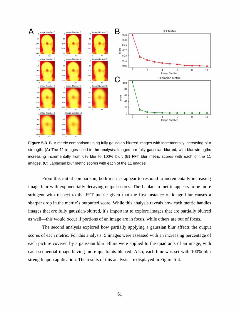
61

Figure 5-3. Blur metric comparison using fully gaussian-blurred images with incrementally increasing blur

strength. (A) The 11 images used in the analysis. Images are fully gaussian-blurred, with blur strengths

increasing incrementally from 0% blur to 100% blur. (B) FFT blur metric scores with each of the 11

images. (C) Laplacian blur metric scores with each of the 11 images.

From this initial comparison, both metrics appear to respond to incrementally increasing

image blur with exponentially decaying output scores. The Laplacian metric appears to be more

stringent with respect to the FFT metric given that the first instance of image blur causes a

sharper drop in the metric’s outputted score. While this analysis reveals how each metric handles

images that are fully gaussian-blurred, it’s important to explore images that are partially blurred

as well—this would occur if portions of an image are in focus, while others are out of focus.

The second analysis explored how partially applying a gaussian blur affects the output

scores of each metric. For this analysis, 5 images were assessed with an increasing percentage of

each picture covered by a gaussian blur. Blurs were applied to the quadrants of an image, with

each sequential image having more quadrants blurred. Also, each blur was set with 100% blur

strength upon application. The results of this analysis are displayed in Figure 5-4.

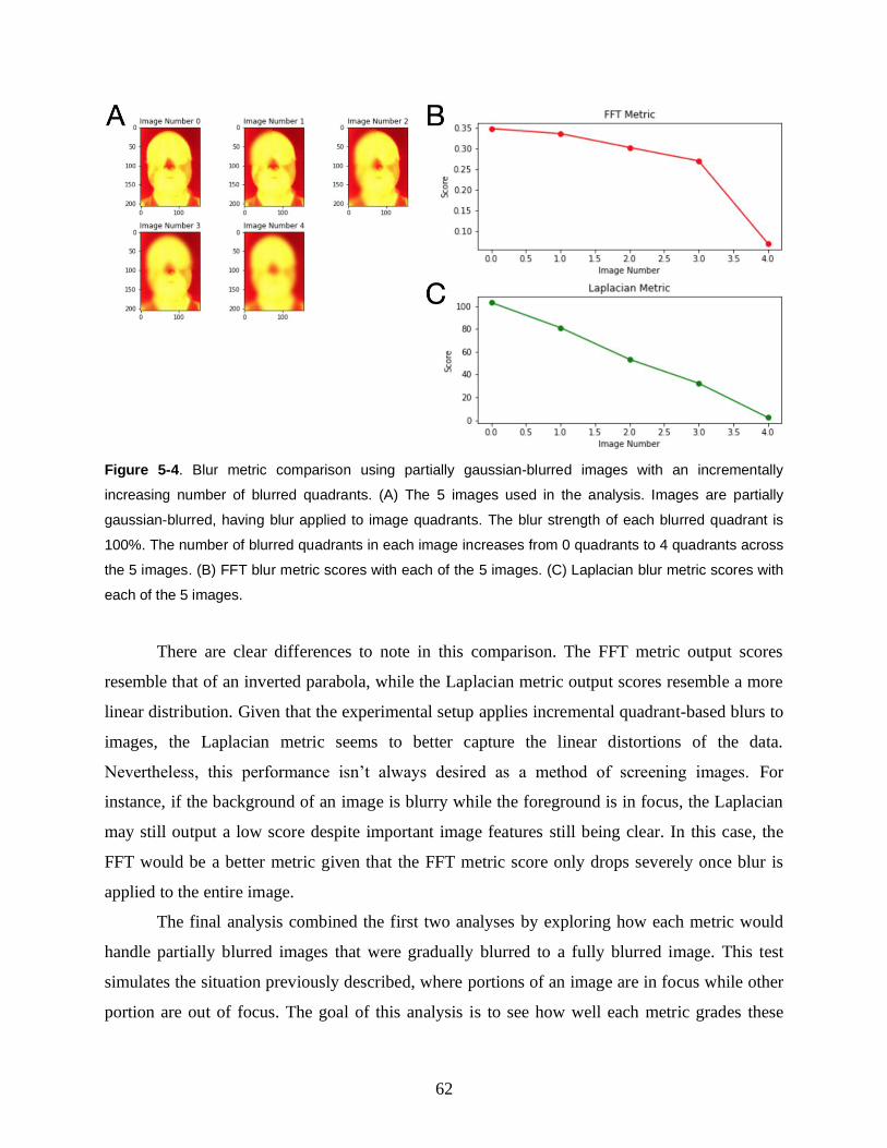
62

Figure 5-4. Blur metric comparison using partially gaussian-blurred images with an incrementally

increasing number of blurred quadrants. (A) The 5 images used in the analysis. Images are partially

gaussian-blurred, having blur applied to image quadrants. The blur strength of each blurred quadrant is

100%. The number of blurred quadrants in each image increases from 0 quadrants to 4 quadrants across

the 5 images. (B) FFT blur metric scores with each of the 5 images. (C) Laplacian blur metric scores with

each of the 5 images.

There are clear differences to note in this comparison. The FFT metric output scores

resemble that of an inverted parabola, while the Laplacian metric output scores resemble a more

linear distribution. Given that the experimental setup applies incremental quadrant-based blurs to

images, the Laplacian metric seems to better capture the linear distortions of the data.

Nevertheless, this performance isn’t always desired as a method of screening images. For

instance, if the background of an image is blurry while the foreground is in focus, the Laplacian

may still output a low score despite important image features still being clear. In this case, the

FFT would be a better metric given that the FFT metric score only drops severely once blur is

applied to the entire image.

The final analysis combined the first two analyses by exploring how each metric would

handle partially blurred images that were gradually blurred to a fully blurred image. This test

simulates the situation previously described, where portions of an image are in focus while other

portion are out of focus. The goal of this analysis is to see how well each metric grades these

63

images when incremental blur is applied to the in-focus section of each image. For this analysis,

test images were created by applying a gaussian blur to the left half of image, where the blur

strength was at 100%. Gaussian blurs of 20% strength were then incrementally added to the right

half of each sequential image, producing 6 images in total. Finally, the original image (with no

blur applied) was included as image number 0, to establish a baseline to compare the results of

this analysis with each metric’s output score for the original image. In all, 7 images were

assessed for this analysis, and the results are displayed in Figure 5-5.

Figure 5-5. Blur metric comparison using partially gaussian-blurred images that were gradually blurred to

a fully blurred image. (A) The 7 images used in the analysis. Besides image number 0, each image

applied a gaussian blur to its left half, where the blur strength was at 100%. Gaussian blurs of 20%

strength were then incrementally added to the right half of each sequential image. (B) FFT blur metric

scores with each of the 7 images. (C) Laplacian blur metric scores with each of the 7 images.

The results from this final comparison mimic the results from the first two analyses. The

FFT metric output score appears to gradually decrease when only some portions of an image

contain blur, but declines sharply once any level of blur is applied to the whole image. The

Laplacian metric output score appears to decrease linearly when only some portions of an image

contain blur, but also declines sharply once any level of blur is applied to the whole image. It is

apparent that both the FFT and Laplacian blur metrics present appropriate descending trends

when analyzing increasingly blurred photos. Nevertheless, the Laplacian metric consistently

64

appears to be the more stringent metric. Between the two metrics, it seems that the FFT metric is

generally better able to account for the sharper portions of images.

The employment of either the FFT or Laplacian metric seems to depend on the problem

attempting to be solved and the image data required. If images contain a background and

foreground, and only certain regions must remain in focus for model performance to be effective,

then the FFT metric seems better suited. If the import features of an image constitute the entire

image, then very little blur should be tolerated, making the Laplacian metric more effective.

Given the nature of the patient image data (Figure 5-1), there is often a background present

which is not essential for the Mobile Technology Group’s classification models. With this in

mind, the FFT metric would be the best blur metric to screening patient images—fine tuning the

high-frequency threshold can somewhat increase the metric’s stringency if necessary.

5.2 Automated Detection of Saturation

The saturation detection problem is actually a simpler task in comparison to the blur detection

problem. A common method of analyzing natural images for whether they are

overexposed/underexposed is by measuring the percentage of ‘dark’ and ‘bright’ pixels in the

image. This analysis allows for the quick detection of whether an image contains a majority low-

intensity or high-intensity pixels. Unfortunately, this method of testing only applies to natural

images, mainly because pixel values within synthetic images don’t necessarily correlate to

saturation—however this is not an issue within the scope of the Mobile Technology Group’s

patient image measurements.

To evaluate the described saturation detection method, a means of separating results is

necessary—this will allow for the creation of ‘underexposed’, ‘normal’, and ‘overexposed’

labels. A potential method is to create a range of pixel intensities that define a ‘normal’ image—

this range will vary depending on the type of image data being analyzed. The initial analysis

examined a patient iris image with varied levels of saturation applied to it—the exposure filters

where applied using Photoshop. A total of 5 images were examined with saturation levels

increasing from -100% strength to 100% strength. The results of the initial analysis are shown in

Figure 5-6—again, all analyses were performed on black and white versions of the input images.

The reason thermal images were not used again for the saturation analysis is because saturation

65

is not relevant in thermal imaging given that thermal cameras do not detect visible light.

However, the methodologies described in this analysis can be repurposed analyze abnormal heat

signatures in thermal images.

Figure 5-6. Saturation metric applied to an iris image at varied saturation levels. The top row of the figure

displays the same iris image with incrementally increasing saturation (ranging from -100% strength to

100% strength). Under each image is the image’s distribution of pixel intensities. Mean values which fall

in the range of a ‘normal’ image are illustrated in green, while mean values that fall outside this range are

illustrated in red. The ‘normal’ range used for this analysis was [97.5, 157.5].

Figure 5-6 also highlights one of the major concerns around the saturation problem, with

regard to conducting image-based analyses, known as clipping. In both Image Number 0 and

Image Number 4, the variance of the pixel values within the image decreases due pixel values

butting up against the bounds of their dynamic range. This creates a loss in information which

cannot be regained via normal color-correcting means. Analyzing an images pixel distribution

allows one to detect potential instances of clipping.

While this method appears to function well with iris image data, there are complications

applying the same methodology to retina image data. Since retina images collected by the

Mobile Technology Group are taken using the Remidio Fundus Camera[6], the majority of the

background is pure black. This greatly skews the distribution of pixel intensities to the right,

which may render the metric ineffective. The naïve solution to correct this issue would be to

recalibrate the ‘normal’ range to account for this shift; however, the percent of a retina image

that is occupied by background varies from image to image—therefore, the amount by which the

66

distribution will shift will also vary. Nevertheless, this problem can be mitigated by simply

excising the lowest intensity values from the distribution, which essentially removes all the

background values from the intensity distribution (Figure 5-7). Overall, this procedure for

analyzing images for saturation is effective across all current patient image data types.

Figure 5-7. Saturation metric and situational corrections applied to a retina image. (A) The original retina

image. (B) The applied saturation detection metric with specific intensities removed from each pixel

intensity distribution. Mean values which fall in the range of a ‘normal’ image are illustrated in green, while

mean values that fall outside this range are illustrated in red. The ‘normal’ range used for this analysis

was [97.5, 157.5]. (C) A representation of the input image entering the saturation detection metric within

each case. For visualization purposes, pixels that were removed from the intensity distribution were

replaced with pixels of maximum intensity (255) in the images. Images depicted are in grayscale due to

being post-analysis outputs (metric inputs are greyscale images).

68

Chapter 6

Diabetes Questionnaire Analysis

Besides patient image data, the main source of data collection for the diabetes screening mobile

application is questionnaire data. There are numerous questionnaires for which patients are asked

to self-report including questionnaires about anxiety, sleep, preservative thinking, depression,

and lifestyle habits relevant to diabetes diagnosis. This analysis will specifically look at the

Diabetes Questionnaire, which assesses the direct risk factors related to diabetes development—

these risk factors are discussed in Chapter 2. The purpose of this analysis is to detect patterns in

the data that can be leveraged by prediction models, potentially leading to simpler solutions

which still enable high predictive power.

Similarly, these patterns may reveal a set of features that can be used to label patients

with different diabetic stages. The Mobile Technology Group does not track the gold-standard

blood tests discussed in Chapter 2; therefore clusters within the data can potentially be used as a

proxy for different diabetic stages if said clusters correlate with diabetes progression.

6.1 Data Preprocessing

In order to conduct meaningful analyses with the questionnaire data, all of the patient’s answers

must be converted into a numerical representation. The Diabetes Questionnaire asks multiple

questions which vary in structure. Some questions require specific numerical answers, such as

queries about height, weight, blood pressure, etc. Some questions are multiple choice, requiring

yes/no responses or a select prompt from a set of options. Finally, the rest of the questions are

multiple select, in which patients are able to select all answers that apply within the bounds of

the question. While the numerical questionnaire data did not need a transformation applied, the

categorical data needed to be encoded into a numerical space.

69

For multiple choice questions, values were assigned using integer encoding, where each

answer choice was assigned an integer value ranging from 0 to the total number of choices.

Higher numbers were generally associated with answer choices which provided more

information and enabled efficient pattern detection in the data—nevertheless, the integer

assignment process was subjective and may be an area of improvement. For multiple select

questions, values were converted using a custom binary instance encoding. Each answer choice

within a question was assigned a digit placement (i.e. ones, tens, hundreds, etc.)—the number of

digit placements matched the total number of choices. Again, answer choices which provided

more information were generally associated with higher digit placements. For the specific set of

answer options which a patient selected for a given question, the digit placement value of each

associated option would be 1, indicating that the choice was selected. The remaining choices

would have digit placement values of 0 to indicate that those choices were not selected.

Therefore, every possible set of selected choices produces a unique string of 0s and 1s

representing a binary number. This binary number was then converted to a base 10 integer to

produce a numerical representing the patient’s answer for said question. More information

regarding how each question in the Diabetes Questionnaire was converted to a numerical value is

provided in Table 6-1.

Question Conversion

Method Original Answer Choice Assignment

1 Height None Decimal Decimal

2 Weight None Decimal Decimal

3 Systolic Blood Pressure None Integer Integer

4 Diastolic Blood

Pressure None Integer Integer

5 Waist Circumference None Decimal Decimal

6 Hip Circumference None Decimal Decimal

7 Have you ever been tested for diabetes?

Integer Encoding

Yes 2

No 1

I don’t know 0

8 Have you ever been

diagnosed with Integer Encoding

Yes 2

No 1

70

diabetes? I don’t know 0

9

If you have been diagnosed with

diabetes, do you know which type of diabetes

you have?

Integer Encoding

Yes, Type 2 Diabetes 3

Yes, Type 1 Diabetes 2

I don’t know 1

N/A 0

10

If you have been diagnosed with

diabetes, when were you diagnosed?

Integer Encoding

More than 15 years ago 7

11-15 years ago 6

6-10 years ago 5

2-5 years ago 4

1-2 years ago 3

7-12 months ago 2

0-6 months ago 1

N/A 0

11 If you have diabetes,

what treatments are you using for your diabetes?

Custom Binary Instance Encoding

Ayurvedic or non-allopathic medicine

7th digit

Tablets 6th digit

Insulin 5th digit

Diet 4th digit

Exercise 3rd digit

No treatment 2nd digit

N/A 1st digit

12 Do you have a family history of diabetes?

Integer Encoding

Yes, both parents 3

Yes, one parent 2

No 1

I don’t know 0

13 Have you ever been

diagnosed with any of these diseases?


Cardiovascular disease 9th digit

Hypertension 8th digit

Anemia 7th digit

Renal or kidney disease 6th digit

Thyroid disease 5th digit

Pulmonary disease (COPD, Asthma, TB, ILD)

4th digit

Cancer 3rd digit

Other 2nd digit

71

N/A 1st digit

14

Besides diabetes medication, are you

also taking medicine for other diseases also?


Cardiovascular disease 11th digit

Hypertension 10th digit

Anemia 9th digit

Renal or kidney disease 8th digit

Thyroid disease 7th digit

Pulmonary disease (COPD, Asthma, TB, ILD)

6th digit

Pain 5th digit

Sleep 4th digit

Cancer 3rd digit

Other 2nd digit

N/A 1st digit

15 How much physical exercise do you do?

Integer Encoding

I do vigorous physical exercise at my work or

outside work on most days 3

I do some (moderate) physical exercise at my

work or outside work 2

I do a little bit (mild) physical exercise at my

work or outside work 1

I have no physical exercise at my work or outside work

0

16 What is your usual diet? Integer Encoding

Vegetarian 2

Vegan 1

Non-veg (My diet includes meat)

0

17 How often do you drink

alcohol? Integer Encoding

Often (more than 2 times per week)

3

Seldom (1 time per week or less)

2

Never 1

Prefer not to answer 0

18

Over the past 2 weeks, how often do you have

difficulty sleeping or difficulty falling asleep?

Integer Encoding

Nearly every day 3

More than half of the days 2

A few days 1

72

Not at all 0

19

Over the past 2 weeks, how often have you

been feeling nervous, anxious, or worried about many things?

Integer Encoding

Nearly every day 3


A few days 1

Not at all 0

20

Over the past 2 weeks, how often have you

been sad, depressed or hopeless?

Integer Encoding

Nearly every day 3


A few days 1

Not at all 0

21 Do you often feel

fatigued? Integer Encoding

Yes 2

No 1

I don’t know 0

22 Approximately how

many times per day do you urinate?

Integer Encoding (Modified)

More than 10 15

8-10 9

6-7 6.5

5 5

4 4

3 3

2 2

1 1

23 Do you often feel pain

in your limbs? Integer Encoding

Yes 2

No 1

I don’t know 0

24 Do you often feel numbness in your

limbs? Integer Encoding

Yes 2

No 1

I don’t know 0

Table 6-1. Numerical conversions applied to the Diabetes Questionnaire patient data.

Along with these questions, additional features were added to assess trends in patient

data—these features included a numerical value representing a patient’s body-mass index (BMI),

a patient’s label for hypertension severity, and a patient’s Indian Diabetes Risk Score (IDRS)

measurement. Each patient’s BMI was calculated using equation 6.1. The hypertension severity

73

label was determined using the American Heart Association’s (AHA’s) guidelines for the

detection, prevention, management, and treatment of high blood pressure[83]. Based on these

guidelines, patients were categorized into one of five hypertension severity levels: normal,

elevated, stage 1, stage 2, and hypertensive crisis. The IDRS is a measurement, created by the

Madras Diabetes Research Foundation (MDRF), designed to aid in the detection of undiagnosed

type 2 diabetes[84]. The IDRS calculation takes in patient features like age, biological sex, waist

circumference, physical activity level, and a patient’s potential family history of diabetes to

output a score which represents the patient’s risk of having or developing diabetic symptoms—

outputted scores are multiples of 10 ranging from 0 to 100. A research study conducted by

Dudeja and coauthors concluded that IDRS values correlate strongly with the presence of type 2

diabetic symptoms, and that the IDRS can be used as a non-invasive measure for diabetes

screening[84]. Numerical conversions for these derived features are shown in Table 6-2.

Question Conversion

Method Original Answer Choice Assignment

1 BMI None Decimal Decimal

2 Hypertension Severity Integer Encoding

Hypertensive Crisis 4

Hypertension: Stage 2 3

Hypertension: Stage 1 2

Elevated 1

Normal 0

3 IDRS (risk score) None Integer Integer

Table 6-2. Numerical conversions applied to features derived from Diabetes Questionnaire patient data.

6.2 Heatmap Correlation Analysis

From Dudeja et al.’s study, it seems likely that patient IDRS values should correlate strongly

with patient random blood sugar (RBS) measurements, especially since abnormal blood sugar

levels are a strong indicator of diabetes manifestation and severity. With this in mind, Figure 6-1

74

was created to display the RBS-IDRS correlation, as well as reveal other patterns that can be

found throughout the Diabetes Questionnaire data. As mentioned before, any patterns/clusters

found in the Diabetes Questionnaire data could be leveraged for patient labeling. This figure was

created by taking all the features within the Diabetes Questionnaire, the features derived from the

Diabetes Questionnaire (BMI, hypertension severity, and IDRS), and each patient’s RBS

measurement and associated RBS measurement instrument (as an integer encoding)—this

created a total of 174 patients and 29 features. All data values were then scaled such that each

feature had unit variance—values ranging between 0 and 1—and the created data table was

plotted in the form of a heatmap.

Figure 6-1. Heatmap analysis of 29 patient features across 174 patients. (A) The heatmap is sorted by

‘RBS’ values in descending order (from top to bottom). (B) The heatmap is sorted by ‘Diabetes

Treatments’ values in descending order (from top to bottom).

Figure 6-1A displayed the heatmap data sorted by each patient’s RBS value. Surprisingly

enough, the figure showed that there is little-to-no correlation between RBS and IDRS values

within the dataset. In fact, Figure 6-1A revealed that there are no observable correlations

between RBS and any of the other features in the data. Given that both RBS and IDRS are

verified methods of screening for diabetes, this discrepancy implied that some underlying patient

feature may be influencing other patient feature values in an unpredicted manor.

75

A trend in the data was eventually observed once patients were sorted by their diabetes

treatment information (Figure 6-1B). In Figure 6-1B, there is a correlation shown at the bottom

of the figure across specific patient features: ‘Tested for Diabetes’, ‘Diagnosed with Diabetes’,

‘Diabetes Type’, ‘Diagnosis History’, and ‘Diabetes Treatments’. Further inspection unearthed

the meaning behind this apparent correlation: these values would all be related for patients whom

have never been tested for diabetes. To elaborate, these untested patients would have also not

been diagnosed, they would not have a diabetes type without a diagnosis, they would also not

have a diagnosis history, and finally they would have no reason to be taking diabetes

medications.

Nevertheless, further analyses were conducted on the patients who were not taking

diabetes medications nor undergoing treatment. This is because the most common form of

medication taken among the patient population was discovered to be metformin (tablets), which

is designed to control blood sugar levels[85]. This discovery invalidates the methodology of using

RBS measurements as a metric for diabetes severity. However, patient RBS measurements could

still be as a valid metric within the subset of patients that are not undergoing diabetes treatments.

With this in mind, a heatmap similar to the one presented in Figure 6-1A was created, but only

with the 24 patients who were not undergoing diabetes treatments (Figure 6-2).

76

Figure 6-2. Heatmap analysis of 29 patient features across 24 patients who have not undergone any

diabetes treatments. The heatmap is sorted by ‘RBS’ values in descending order (from top to bottom).

Figure 6-2 appears to display moderate correlations within the data, which is an

improvement from the results depicted in Figure 6-1A—it appears that blood pressure, waist and

hip circumference, and risk score generally increases as RBS increases. If the patient risk scores

correlate strongly with the patient RBS values among the 24-patient population, it’s possible that

the IDRS metric could be used as a proxy for classifying diabetes within the whole 174-patient

population (since RBS is not usable with medicated patients). The reason why the IDRS would

be usable is because IDRS values are not significantly affected by patient medical treatments. An

77

IDRS value is computed from patient lifestyle-based questions rather than biomolecular

measurements—therefore IDRS would make an excellent proxy for the whole dataset if

applicable. Figure 6-3 was created to examine the validity of using IDRS as a proxy. The figure

displays a scatter plot showing the relationship between RBS and IDRS within the 24-patient

population. Table 6-3 complements Figure 6-3 by presenting the correlation coefficients from

both Pearson and Spearman correlation metrics.

Figure 6-3. Scatterplot depicting the correlation between RBS and IDRS among the 24 untreated patients

in the 174-patient population.

78

Correlation Metric Correlation Coefficient P-value

Pearson Correlation 0.436 0.033

Spearman Correlation 0.538 0.007

Table 6-3. Pearson and Spearman correlation coefficients for the correlation between RBS and IDRS

among the 24 untreated patients in the 174-patient population. The coefficients from both the Pearson

and the Spearman metric imply that there is a moderate correlation between the two features. With a

significant threshold of α=0.05, both coefficients are statistically significant.

The results shown in Figure 6-3 and Table 6-3 show that there is a moderate correlation

between the RBS values and IDRS values among the untreated population of patients, which

aligns with the initial assumption that IDRS is an effective diagnostic for diabetes severity. From

this analysis, it’s clear that the questionnaire is not fine-tuned to detect signals of diabetes in

medicated patients. So far, the IDRS is the only patient feature which may correlate strongly

with diabetic severity. To improve the Diabetes Questionnaire’s efficacy, further research must

be conducted on diabetic symptoms that are still detectable when undergoing each type of

diabetes treatment currently available—this will allow for more tailored questions which reveal

useful information across all patients. Additionally, collecting more patient data from patients

whom are not undergoing treatments would improve the statistical power of the RBS-IDRS

correlation analyses presented in Figure 6-3 and Table 6-3.

Since the IDRS score appears to correlate with diabetic severity, and the IDRS is derived

from other patient features within the Diabetes Questionnaire, there may be underlying patterns

in the patient data that are unable to be detected via various ordered sorts. Chapter 7, will discuss

the extent by which machine learning frameworks are able to uncover these patterns and leverage

them for the prediction of different diabetic stages.

80

Chapter 7

Semi-Supervised Autoencoder for Patient Labeling

A major limitation of the current dataset for the diabetes screening mobile application is that

patients are not labeled for diabetic severity—this means they aren’t labeled for the

presence/absence of diabetic symptoms, nor are they labeled under the specific diabetic stages

discussed in Chapter 2. For any supervised machine learning model to function, the model must

be provided with ground truth labels for training (in terms of what the model will be predicting).

Since, the end goal for the mobile application is to be able to output a label depicting the stage of

diabetes which a patient is in, there is interest in developing a method to label each measurement

with respect to specific diabetic stages.

The best method to label this medical data is by a physician who is an expert in diabetes.

However, with an increasing amount of patient data being collected for the mobile application,

the workload necessary to label this data manually is unreasonable. Nevertheless, there are

computational techniques that are able to utilize a small set of labels in order to classify/label

whole datasets of patients. This chapter will the discuss how a semi-supervised autoencoder can

be employed for the task of patient labeling.

7.1 Motivation Behind the Semi-Supervised Autoencoder and Initial

Assumptions

The reason a semi-supervised autoencoder was selected for the task was because while the model

aims to improve classification of the data, the model also attempts to maintain the data’s

representation—this both helps to prevent overfitting on the training data, and it ensures that

classification is done using meaningful features and values from the training data. Nevertheless,

the semi-supervised autoencoder will only produce meaningful results on the basis that three

81

major assumptions about the data remain true: the continuity assumption, the cluster assumption,

and the manifold assumption[86].

Firstly, the continuity assumption postulates that points which are close to each other are

more likely to share a label. This means it’s expected that patients that share similar values with

respect to their input features are expected to be in similar diabetic stages. Secondly, the cluster

assumption postulates that datapoints tend to form discrete clusters, and points within the same

cluster are more likely to share a label. Like the continuity assumption, patients with similar

feature values are expected to be near each other. These patients would then form clusters,

ideally displaying the distinct diabetic stages represented within the patient population. Finally,

the manifold assumption postulates that distinctive feature information within the data lies on a

manifold of much lower dimension than the input space. This means that the patient data can be

encoded into a lower dimensional representation while still preserving important feature

distinctions. This would allow for the autoencoder to learn patterns based on these encoded

patient features, rather that learn on a noisy and complex input space.

7.2 Methods

7.2.1 Autoencoder Input Features

There are multiple sources of data by which the autoencoder can extract features from including

patient image data and questionnaire data; however, there are limitations to what data would

actually enhance the model. For instance, patient images data is very valuable, but important

features must be extracted from image data prior to model input in order to provide useful

information. While images are able to be included as direct inputs into an autoencoder, the

competing classification task and decoding task of the semi-supervised learning system would

make feature extraction less efficient. The Mobile Technology Group is currently developing

algorithms and models to effectively extract relevant features from the patient image data; these

outputs can then be incorporated into the autoencoder to improve the autoencoder’s performance.

Nevertheless, features related to image data—including thermal, iris, and retina images—will

have to be excluded for this initial analysis of the autoencoder.

The remaining patient data includes blood test measurements, visual acuity test

measurements, and patient questionnaire data, which would all be effective as direct inputs into

82

the autoencoder model in a general context. However, specific complications made certain

features unusable for this initial analysis. For instance, blood test measurements were excluded

because a majority of the patient population was undergoing diabetic treatments via

medication—as depicted in Chapter 6, medicated patients don’t have blood sugar levels that

correlate with diabetic symptoms. Since the dataset has more patients on medication than without

medication, the addition of blood test measurements would provide more noise for the model

than useful information.

Some measurement features were disregarded because a significant number of patients

had not yet taken the specified measurement tests. Without a high volume of patient data, all

analyses must be conducted using only completed patient feature vectors—this is because

missing values in the data cannot be interpolated without an abundance of other patient data to

form a baseline. Therefore, only patients who have completed all the measurement tests, which

were used as input features, could be included in the autoencoder analysis; this limited the

number of measurement tests that could be used in order to maintain a sufficient number of

patients.

Ultimately, in order to maximize the number of patients and the number of patient

features included in this initial analysis, only the Diabetes Questionnaire data was used to create

the autoencoder input features. From the Diabetes Questionnaire, 25 essential features were

extracted for use in the analysis. The inclusion of any other measurement tests would not have

allowed for a multiclass prediction—this experimental setup will be described further in Sections

7.2.2 and 7.2.3. With the inclusion of more patient data, across more measurement tests in

general, a stronger and more robust analysis can be completed in the future.

7.2.2 Ground Truth Label Formation

Despite the autoencoder being designed for the task of labelling patients, the model would be

unable to train without a small sample of patient labels—this is necessary for the supervised

aspect of the semi-supervised autoencoder. A “small sample” of labels is a loose definition: at

least one unique class label is necessary for every class for which the model is attempting to

predict, and the accuracy of the model increases with the more labels within each class.

As previously mentioned, none of the patients within the dataset are clinically labeled so

a proxy must be used to conduct this analysis. As concluded in Chapter 6, patient IDRS values

83

make a fairly good proxy for labeling patients under different diabetic states. For this analysis,

IDRS values were used to label patients under three classes: Class 0 (non-diabetic), Class 1

(prediabetic), and Class 2 (diabetic). The reason for this is three class system rather than the ideal

six class system is due to the limitations of using IDRS values—IDRS values have no distinct

metric for classifying each of the unique diabetic stage, but the values can be used to classify

patients into low risk, medium risk, and high risk groups. The low risk group corresponds to

Class 0 which spans risk scores in the range [0, 30), the medium risk group corresponds to Class

1 which spans risk scores in the range [30, 60), and the high risk group corresponds to Class 2

which spans risk scores in the range [60, 100]. All patients were labeled under one of these

designated diabetic classes based on this criteria.

7.2.3 Autoencoder Hyperparameters and Architecture

The autoencoder was designed as a five-layer feed-forward neural network, with two encoding

layers (an input layer and a hidden layer), two decoding layers (a hidden layer and an output

layer), and a softmax classification layer attached to the latent encoded layer (Figure 7-1). Given

that each patient has 25 features within their feature vector the length of the input layer is 25

units; this also means that the length of the output layer is 25 units. Each hidden layer has a

length of 10 units. The encoded layer is designed to be 2 units in length in order to produce a

two-dimensional encoding for each patient—the dimensionality of the encoding is does not

strictly need to be 2; however this setup allows for the dimensionality reduction analysis to be

conducted using a 2D cartesian plane. The length of the classification layer of the autoencoder

depends on the number of classes that the autoencoder will be classifying patients into. There are

three diabetic classes in this preliminary analysis, so the classification layer is 3 units long.

Besides the classification layer, all layers within the autoencoder were activated by the sigmoid

activation function. The autoencoder was created using Python and the TensorFlow Python

library (version 2.1.0).

84

Figure 7-1. Semi-supervised autoencoder architecture.

The autoencoder was trained using both the mean absolute error and the categorical

cross-entropy loss functions, having both lasso and ridge regularization applied as well. The

mean absolute error loss function was used for the decoding task while the categorical cross-

entropy loss function was used for the classifying task. The model was trained using mini-batch

gradient descent with 2,000 epochs and batch sizes of 10 patients.

In total, there were 212 patients included in this analysis: 2 patients in Class 0, 48 patients

in Class 1, and 162 patients in Class 2. A 50/50 split was applied to the dataset to produce a

training dataset and a testing dataset for the autoencoder’s creation and evaluation, and the

division of the patient data is highlighted in Figure 7-2. The original dataset was randomly

shuffled prior to the 50/50 split, so each patient had an equal chance of being in either the

training or testing dataset.

85

Figure 7-2. Division of 212 patients into training and testing datasets via 50/50 split.

7.2.4 Dimensionality Reduction Analysis

As discussed in Section 7.1, there are many assumptions which are being taken in the process of

developing the semi-supervised autoencoder. This dimensionality reduction analysis is designed

to confirm whether these assumptions hold true within the dataset of patients used for the

creation and evaluation of the autoencoder.

The encoded layer of the autoencoder provides the autoencoder’s representation of the

patient data in a two-dimensional space. If the assumptions hold true, and the design of the

autoencoder is effective, then the 2D patient representations produced by the autoencoder should

ideally produce three distinct clusters which correlate to the three unique ground truth labels. The

dimensionality reduction analysis determined whether the autoencoder’s representation matched

this expected result by performing a k-means clustering of the autoencoder’s 2D patient

representation. This clustering was then compared to an identical representation where clusters

assignments were based on ground truth labels—as previously mentioned, the clusters in both

representations should be identical under the correct conditions. Given that there are three unique

classes within the dataset, k-mean clustering was completed using three clusters (k=3).

To also analyze the strength of the autoencoder’s 2D patient representations, the same

dimensionality reduction analysis was conducted on 2D patient representations using PCA (a

linear dimensionality reduction method) and t-SNE (a non-linear dimensionality reduction

86

method) as controls. The average silhouette coefficient of the ground truth clusters was used to

quantifiably evaluate the quality of each methods dimensionality reduction. All of the analyses

were conducted only using the 106 patients that were in the testing dataset. The k-means

clustering, PCA, t-SNE, and silhouette coefficient operations were completed using the scikit-

learn Python library (version 0.21.3)—the perplexity of t-SNE was set to 20.

7.3 Results

7.3.1 Patient Labeling via Autoencoder

The results of the autoencoder’s classification task can be seen in Figure 7-3 and Figure 7-4

displaying the receiver operator characteristic (ROC) curve and the precision-recall curve of the

binarized multi-class autoencoder predictions, respectively. As depicted in the legend of Figure

7-3, the areas under the ROC (AUROCs) curves for the binarized class predictions depict

positive performance of the overall model. The AUC of the binarized Class 0, however, is

misleading due to the fact that there was only one patient in Class 0 within the testing dataset—

nevertheless, the model predicted the patient’s class correctly.

The legend of Figure 7-4 shows the areas under the precision recall (AUPRs) curves for

the binarized class predictions. There is mixed performance among the different classes, but

there is an apparent trend in that the more samples which the autoencoder is trained on for a

given class, the higher the autoencoder’s positive predictive value is for that class. The exception

for this is the model’s apparent predictive power for Class 0. Again, the AUPR of the binarized

Class 0 is misleading due to the fact that there was only one patient in Class 0 within the testing

dataset. The addition of more Class 0 patients in future iterations of the semi-supervised

autoencoder analysis will lead to more conclusive results.

7.3.2 Dimensionality Reduction via Autoencoder

The dimension-reduced patient features via autoencoder are shown in Figure 7-5. Upon visual

inspection, there are many differences between the clusters presented in the k-means clustering

of the data and the ground truth clusters. This could mean that either the autoencoder is unable to

properly separate the ground truth clusters due to its design, or the data is not easily separable

because one or more of the fundamental assumptions is untrue.

87

The dimension-reduced patient features via PCA and via t-SNE are shown in Figure 7-6.

These figures display a similar trend in that clusters presented in the k-means clustering do not

coincide with the ground truth clusters. Given that PCA and t-SNE are common and effective

methods to perform dimensionality reduction, these results suggest hat the problem lies in the

data rather than the autoencoder.

The average silhouette coefficients of the original dataset and each dimension-reduced

dataset are displayed in Table 7-1. This table reveals that the autoencoder was best able to cluster

the ground truth variables compared to the original dataset and the control dimensionality

reduction methods.

Figure 7-3. Receiver operating characteristic (ROC) curves of the binarized multi-class predictions of the

semi-supervised autoencoder.

88

Figure 7-4. Precision-recall curves of the binarized multi-class predictions of the semi-supervised

autoencoder.

89

Figure 7-5. Dimensionality reduction of 106 patient feature vectors via autoencoder. (A) K-means

clustering of the dimensionality reduction via autoencoder; k=3. (B) Ground truth clustering of the

dimensionality reduction via autoencoder.

90

Figure 7-6. Dimensionality reduction of 106 patient feature vectors via controls (PCA and t-SNE). The top

two plots display the k-means clustering of the dimensionality reduction (A) via PCA and (B) via t-SNE;

k=3. The bottom two plots display the ground truth clustering of the dimensionality reduction (C) via PCA

and (D) via t-SNE.

91

Dimensionality Reduction Method

Dimensionality of Data Average Silhouette

Coefficient

None 25-dimensional -0.0059

Semi-Supervised Autoencoder 2-dimensional 0.1864

PCA 2-dimensional -0.0798

t-SNE 2-dimensional -0.1043

Table 7-1. Average silhouette coefficients of the ground truth clusters within the original dataset and the

various dimension-reduced patient representations.

7.4 Discussion

The results of the autoencoder’s patient labeling analysis display that model is well-suited to

label patient data despite limited resources. The model shows promise in terms of handling the

multi-class labeling task; however, further analysis is necessary when significantly more patient

data under the other diabetic classes becomes available. The performance of the autoencoder’s

classification implies that there are patterns within the Diabetes Questionnaire data that the

autoencoder was able to leverage for patient labeling, despite the lack patterns observed in the

data in the correlation analyses conducted in Chapter 6. The addition of more data from other

measurement tests may improve the predictive power of the autoencoder in future analyses.

The results of the autoencoder’s dimensionality reduction analysis show that the

autoencoder is unable to separate the patient data into ground truth labels in the lower

dimensional space. However, all the dimensionality reduction methods seem to struggle in

executing this task, which hints that the underlying problem may be within the data. The results

imply that the data does not align with one or more of the assumptions presented in Section 7.1,

meaning that there is too much variation among the patient features for patients within the same

ground truth cluster. This conclusion aligns with conclusions derived in Chapter 6, as the

Diabetes Questionnaire dataset had so much variation to no clear patterns were observable.

The results of the autoencoder’s patient labeling analysis and the results of the

autoencoder’s dimensionality reduction analysis seemingly conflict, because the former implies

that there are patterns in the Diabetes Questionnaire data while the latter implies that there is

mainly noise in the Diabetes Questionnaire data. This contradiction can be explained by the fact

92

that the autoencoder’s classification task can be somewhat successful if the model is able to pick

up on at least one feature that is indicative of the ground truth labels. However, the autoencoder’s

encoding task is only successful if there are patterns across multiple features that are indicative

of the ground truth labels. This conclusion can also be derived from the autoencoder’s encoding

function, which appears to perceive that the data can be split using only a single dimension—this

is why the autoencoder outputs patient datapoints along a diagonal. The only reason the

autoencoder’s 2D encoding would display a 1D solution is if the autoencoder’s classifier

determined that only one feature in the dataset which was indicative of ground truth labels.

Nevertheless, the inclusion of other patient measurements—especially the score from image-

based and PPG-based predictive models—is likely to improve the performance of both the

autoencoder’s tasks.

94

Chapter 8

Conclusion and Future Work

8.1 Contributions of Work

8.1.1 Exploration into the Biological Characteristics of Diabetes and Non-Invasive

Technologies to Detect Them

This thesis discussed the pathology and etiology of CMS with a focus on diabetes, enabling

guided research for the development of new tools—or the repurposing current tools—that detect

diabetic symptoms. Some non-invasive detection tools were explored throughout this thesis as

well, highlighting the potential of non-invasive diabetes diagnostics in easing the burden on the

global health care system. The inclusion of these tools, and the creation of predictive models to

calibrate these tools for the diabetes classification task, would greatly improve the current

diabetes screening mobile application.

8.1.2 Image Quality Metrics for the Improvement of Image-Based Predictive Models

This thesis included a discussion about analyses performed on image quality metrics which can

be employed to screen for high quality patient images. Adding a screen as an additional

preprocessing step would ultimately improve the extraction of important image-based features,

and potentially improve the predictive power of the Mobile Technology Group’s image-based

predictive models.

8.1.3 Preliminary Semi-Supervised Autoencoder for Patient Labeling

This thesis included a discussion about the creation and respective analyses performed on a semi-

supervised autoencoder for the task of labeling patients within the Mobile Technology Group’s

patient database. The discussion included information regarding the complications of using blood

95

sugar measurements with medicated patients, and the need to use patient IDRS values as a proxy

for base the autoencoder’s ground truth labels. The classification aspect of the autoencoder

performed moderately well, with a class-average area under the receiver operator characteristic

(AUROC) of 0.845, and a class-average area under the precision-recall (AUPR) curve of 0.789.

The encoding function developed by the autoencoder was not effective in separating the patient

data into ground truth clusters; nevertheless, the autoencoder was still the most effective method

for clustering the ground truth labels with a silhouette coefficient of 0.1864. With the results of

this preliminary analysis, the autoencoder shows great promise in becoming an effective tool for

patient labeling.

8.2 Future Work

Analyses which explored batches of patient data (Chapter 6 and Chapter 7) would greatly be

improved in terms of statistical power with the addition of more patient data across more

measurement tests; this would enable more meaningful conclusions to be derived from these

analyses. In this vein, it would be beneficial to expand the Diabetes Questionnaire analysis to

other questionnaires once a significant number of patients have taken these measurements—this

is in order to guarantee that analyses are robust. Similarly, it would be important in the future to

collect more data from patients whom are not undergoing medication in order to conduct data

correlation analyses using blood testing measurements. Blood tests are the gold standard

measurements for measuring diabetes progression and enable a more accurate separation of

patients into different diabetic stages.

The culmination of more patient data across different measurement tests, with a balance

of medicated and non-medicated patients among each measurement test, would also greatly

improve the predictive capability of the semi-supervised autoencoder—the autoencoder would be

able to explore more patient features and recognize stronger patterns in the data which are

indicative of each diabetic stage irrespective of the use of medication. The functionality of the

autoencoder would also be truly realized once a subset of patients are classified via direct

physician examination. The proxies used for the preliminary autoencoder defeat the purpose of

the autoencoder—if ground truth labels are created based on a single feature, there would be no

need for a model as long as the patient data for that single feature continues to be collected. The

96

use of blood sugar measurements for labeling would have been viable had the target patient

demographic solely been patients not on medication.

The image quality metrics would benefit from field testing once the predictive models for

each patient image type are finalized. These future analyses would consist of examining whether

models trained using images screened by the quality metrics improved the performance of the

predictive models—this is with respect to models trained using only the excised images as well

as models trained using all patient images. Future work would also include creating quality

metrics for photoplethysmography (PPG) measurements and questionnaire data—the reason

questionnaire data would need a quality metric is because questionnaire can contain aleatoric

error due to misinformation or incorrectly input values. Once quality metrics are developed for

all the relevant measurement tests, it would be useful to develop and implement data correction

methods which improve data of poor quality—this would also increase the number of patients

available for use within various analyses.

Data collection for the mobile application can be improved by using additional non-

invasive technologies as measurements tests—many of which are discussed in Chapter 3. These

diagnostic tests explore different aspects of diabetes pathogenesis and etiology, enabling better

characterization of prediabetic and diabetic stages. The inclusion of measurements from these

additional non-invasive diabetes screening tools could greatly improve the autoencoder’s patient

labeling process, as well as the Bayesian network model developed by Shivani Chauhan—a prior

Masters student of the Mobile Technology Group[6].

8.3 Larger Impact

The work presented in this thesis has been to evaluate and enhance the aspects of data collection,

data processing, and model creation for the Mobile Technology Group’s non-invasive diabetes

screening mobile application. Nevertheless, many of the technologies and analyses presented

throughout this thesis can be scaled to other projects, both within and outside of the Mobile

Technology Group, in the pursuit of developing technologies for non-invasive diagnoses. A

higher goal is to be able to leverage these tools to be able to diagnose the progression of various

umbrella diseases, such as cardiometabolic syndrome (CMS), in order to aid a wider population

of individuals who are still unable to receive proper medical care. Ultimately, it is the hope of

97

our group that this work will galvanize further research into the intricacies of interconnected

conditions in order to bring innovation to biomedical research and technology.

99

Bibliography

[1] World health statistics. World Health Organization, World Health Organization.

www.who.int/gho/world-health-statistics.

[2] Loudenback Tanza. The average cost of healthcare in 21 different countries. Business

Insider, Business Insider. 2019 Mar 7. www.businessinsider.com/personal-finance/cost-of-

healthcare-countries-ranked-2019-3.

[3] Diabetes. World Health Organization, World Health Organization. 2018 Oct 30.

www.who.int/news-room/fact-sheets/detail/diabetes.

[4] Bommer C, et al. Global economic burden of diabetes in adults: projections from 2015 to

2030. Diabetes Care, American Diabetes Association. 2018 May.

https://care.diabetesjournals.org/content/41/5/963.

[5] Yu Tania. Iris imaging for health diagnostics. Master’s thesis, MIT. 2018.

[6] Chauhan Shivani. A mobile platform for non-invasive diabetes screening. Master’s thesis,

MIT. 2019.

[7] Malik Vasanti S, et al. Global obesity: trends, risk factors and policy implications. Nature

Reviews. Endocrinology, U.S. National Library of Medicine. 2013 Jan.

doi.org/10.1038/nrendo.2012.199.

[8] Castro Jonathan P, et al. Cardiometabolic syndrome: pathophysiology and treatment.

Current Hypertension Reports, U.S. National Library of Medicine. 2003 Oct.

doi.org/10.1007/s11906-003-0085-y.

[9] Saljoughian Manouchehr. Cardiometabolic syndrome: a global health issue. U.S.

Pharmacist – The Leading Journal in Pharmacy. 2017 Feb 16.

www.uspharmacist.com/article/cardiometabolic-syndrome-a-global-health-issue.

[10] What is cardiometabolic disease and how is it different from cardiovascular disease?

Health & Nutrition Letter – Your Guide to Living Healthier Longer. 2018 Mar.

www.nutritionletter.tufts.edu/issues/14_3/ask-experts/Q-What-is-cardiometabolic-disease-

and-how_2308-1.html.

[11] Holland Kimberly. 12 leading causes of death in the United States. Medically Reviewed by

Deborah Weatherspoon, Healthline, Healthline Media. 2018 Nov 1.

www.healthline.com/health/leading-causes-of-death.

[12] Statistics about diabetes. American Diabetes Association. 2018 Mar 22.

www.diabetes.org/diabetes-basics/statistics/.

100

[13] The Editors of Encyclopaedia Britannica. Islets of Langerhans. Encyclopædia Britannica,

Encyclopædia Britannica, Inc. 2018 July 11. www.britannica.com/science/islets-of-

Langerhans.

[14] Weir Gordon C, Bonner-Weir Susan. Five stages of evolving beta-cell dysfunction during

progression to diabetes. Diabetes, American Diabetes Association. 2004 Dec 1.

diabetes.diabetesjournals.org/content/53/suppl_3/S16.

[15] Tabák Adam G, et al. Prediabetes: a high-risk state for diabetes development. Lancet

(London, England), U.S. National Library of Medicine. 2012 June 16.

doi.org/10.1016/S0140-6736(12)60283-9.

[16] Ramachandran A. Know the signs and symptoms of diabetes. Indian J Med Res, 2014 Nov;

140(5):579‐581. www.ncbi.nlm.nih.gov/pmc/articles/PMC4311308/.

[17] Hyperinsulinemia. Diabetes.co.uk – The Global Diabetes Community. 2019 Jan 15.

www.diabetes.co.uk/hyperinsulinemia.html.

[18] Saini Vandana. Molecular mechanisms of insulin resistance in type 2 diabetes mellitus.

World Journal of Diabetes, Baishideng Publishing Group Co., Limited. 2010 July 15;

1(3):68‐75. doi.org/10.4239/wjd.v1.i3.68

[19] Mayo Clinic Staff. Prediabetes. Mayo Clinic, Mayo Foundation for Medical Education and

Research. 2017 Aug 2. www.mayoclinic.org/diseases-conditions/prediabetes/symptoms-

causes/syc-20355278.

[20] Sinha Sunil K. Hyperinsulinism workup: laboratory studies, imaging studies, other tests.

Edited by Stephen Kemp, Medscape. 2019 Feb 2. emedicine.medscape.com/article/921258-

workup.

[21] Thiruvengadam, J., Anburajan, M., Menaka, M., Venkatraman, B. Potential of thermal

imaging as a tool for prediction of cardiovascular disease. Journal of Medical Physics.

2014 Apr; 39(2):98‐105. doi.org/10.4103/0971-6203.131283.

[22] Dekker Martijn A M den, et al. Skin autofluorescence, a non-invasive marker for AGE

accumulation, is associated with the degree of atherosclerosis. PloS One, Public Library of

Science. 2013 Dec 23. doi.org/10.1371/journal.pone.0083084.

[23] Ferrante Anthony W. The immune cells in adipose tissue. Diabetes, Obesity & Metabolism,

U.S. National Library of Medicine. 2013 Sep; 15 Suppl 3(0 3):34‐38.

doi.org/10.1111/dom.12154.

[24] WebMD Medical Reference. Are diabetes and inflammation connected? Medically

Reviewed by Michael Dansinger, WebMD, WebMD. 2017 June 21.

www.webmd.com/diabetes/type-2-diabetes-guide/inflammation-and-diabetes#1.

[25] Shoelson Steven E, et al. Inflammation and insulin resistance. The Journal of Clinical

Investigation. 2006 July 3; 116(7):1793‐1801. doi.org/10.1172/JCI29069.

[26] Bornfeldt Karin E, Tabas Ira. Insulin resistance, hyperglycemia, and atherosclerosis. Cell

Metabolism. 2011 Nov 2; 14(5):575‐585. doi.org/10.1016/j.cmet.2011.07.015

[27] Atherosclerosis. National Heart Lung and Blood Institute, U.S. Department of Health and

Human Services, www.nhlbi.nih.gov/health-topics/atherosclerosis.

101

[28] University of Rochester Medical Center. How diabetes drives atherosclerosis.

ScienceDaily, ScienceDaily. 2008 Mar 17.

www.sciencedaily.com/releases/2008/03/080313124430.htm.

[29] What is type 1 diabetes? Joslin Diabetes Center, 2019.

www.joslin.org/info/what_is_type_1_diabetes.html.

[30] Cantley James, Ashcroft Frances M. Q&A: insulin secretion and type 2 diabetes: why do β-

cells fail? BMC Biology. 2015 May 16. doi.org/10.1186/s12915-015-0140-6

[31] Hess-Fischl Amy. Hyperglycemia: when your blood glucose level goes too high. Medically

Reviewed by Brigid Gregg, EndocrineWeb. 2018 Sep 7.

www.endocrineweb.com/conditions/hyperglycemia/hyperglycemia-when-your-blood-

glucose-level-goes-too-high.

[32] Diagnosing diabetes and learning about prediabetes. American Diabetes Association. 2016

Nov 21. www.diabetes.org/diabetes-basics/diagnosis/.

[33] Prediabetes. Wikipedia, Wikimedia Foundation. Accessed: 2019 Apr 10.

en.wikipedia.org/wiki/Prediabetes.

[34] Mayo Clinic Staff. Hyperglycemia in diabetes. Mayo Clinic, Mayo Foundation for Medical

Education and Research. 2018 Nov 3. www.mayoclinic.org/diseases-

conditions/hyperglycemia/symptoms-causes-syc-20373631.

[35] Aronson Doron, Rayfield Elliot J. How hyperglycemia promotes atherosclerosis: Molecular

Mechanisms. Cardiovascular Diabetology, BioMed Central. 2002 Apr 8.

cardiab.biomedcentral.com/articles/10.1186/1475-2840-1-1.

[36] Jezovnik Mateja K, Poredos Pavel. Oxidative stress and atherosclerosis. European Society

of Cardiology. 2007 Oct 9. www.escardio.org/Journals/E-Journal-of-Cardiology-

Practice/Volume-6/Oxidative-stress-and-atherosclerosis-Title-Oxidative-stress-and-

atheroscleros.

[37] Wisse Brent. Diabetic ketoacidosis. Medically Reviewed by David Zieve, MedlinePlus,

U.S. National Library of Medicine. 2018 Jan 16. medlineplus.gov/ency/article/000320.htm

[38] Galan Nicole. 9 early warning signs and symptoms of type 2 diabetes. Medically Reviewed

by Maria Prelipcean, Medical News Today, MediLexicon International. 2018 Sep 26.

www.medicalnewstoday.com/articles/323185.php.

[39] Mayo Clinic Staff. Diabetes. Mayo Clinic, Mayo Foundation for Medical Education and

Research. 2018 Aug 8. www.mayoclinic.org/diseases-conditions/diabetes/symptoms-

causes/syc-20371444.

[40] Mayo Clinic Staff. Heart disease. Mayo Clinic, Mayo Foundation for Medical Education

and Research. 2018 Mar 22. www.mayoclinic.org/diseases-conditions/heart-

disease/symptoms-causes/syc-20353118.

[41] Diabetes, gum disease, & other dental problems. National Institute of Diabetes and

Digestive and Kidney Diseases, U.S. Department of Health and Human Services. 2014 Sep

1. www.niddk.nih.gov/health-information/diabetes/overview/preventing-problems/gum-

disease-dental-problems.

102

[42] Mayo Clinic Staff. Type 2 diabetes. Mayo Clinic, Mayo Foundation for Medical Education

and Research. 2019 Jan 9. www.mayoclinic.org/diseases-conditions/type-2-

diabetes/diagnosis-treatment/drc-20351199.

[43] Al-Lawati J A. Diabetes mellitus: a local and global public health emergency! Oman Med

J. 2017; 32(3):177-179. doi:10.5001/omj.2017.34.

[44] WHO guidelines on hand hygiene in health care: first global patient safety challenge clean

care is safer care. Geneva: World Health Organization, The burden of health care-

associated infection. 2009; 3. Available from: www.ncbi.nlm.nih.gov/books/NBK144030/.

[45] Healthcare-acquired infections (HAIs). PatientCareLink. Massachusetts Health & Hospital

Association. Accessed: 2020 May 5. patientcarelink.org/improving-patient-care/healthcare-

acquired-infections-hais/.

[46] Ring E F J, Ammer K. Infrared thermal imaging in medicine. Institute of Physics and

Engineering in Medicine. 2012. doi.org/10.1088/0967-3334/33/3/R33.

[47] Ring Francis. Thermal Imaging Today and Its Relevance to Diabetes. Journal of Diabetes

Science and Technology. Diabetes Technology Society. 2010 July 1.

doi.org/10.1177/193229681000400414.

[48] Brånemark P, Fagerberg S, Langer L, et al. Infrared thermography in diabetes mellitus a

preliminary study. Diabetologia. 1967; 3:529-532. doi.org/10.1007/BF01213572.

[49] Fushimi H, Inoue T, Nishikawa M, Matsuyama Y, Kitagawa J. A new index of autonomic

neuropathy in diabetes mellitus: heat stimulated thermographic patterns. Diabetes Res.

Clin. Pract. 1985; 1(2):103-107. doi.org/10.1016/S0168-8227(85)80035-8.

[50] Fokkens Bernardina T, Smit Andries J. Skin fluorescence as a clinical tool for non-invasive

assessment of advanced glycation and long-term complications of diabetes. Glycoconjugate

Journal, Springer US. 2016 June 10. doi.org/10.1007/s10719-016-9683-1.

[51] Cahn F, Burd J, Ignotz K, Mishra S. Measurement of lens autofluorescence can distinguish

subjects with diabetes from those without. J Diabetes Sci Technol. 2014 Jan; 8(1):43-49.

doi.org/10.1177/1932296813516955.

[52] Steenbeke M, et al. UV fluorescence-based determination of urinary advanced glycation

end products in patients with chronic kidney disease. Diagnostics. 2020.

doi.org/10.3390/diagnostics10010034.

[53] Paolillo F R, Mattos V S, de Oliveira A O, Guimarães F E G, Bagnato V S, de Castro Neto

J C. Noninvasive assessments of skin glycated proteins by fluorescence and Raman

techniques in diabetics and nondiabetics. J Biophotonics. 2019 Jan; 12(1):e201800162.

doi.org/10.1002/jbio.201800162.

[54] Olson B P, Matter N I, Ediger M N, Hull E L, Maynard J D. Noninvasive skin fluorescence

spectroscopy is comparable to hemoglobin A1c and fasting plasma glucose for detection of

abnormal glucose tolerance. J Diabetes Sci Technol. 2013 July 1; 7(4):990-1000.

doi.org/10.1177/193229681300700422.

[55] Type 2 diabetes risk test. American Diabetes Association. www.diabetes.org/risk-test.

103

[56] Tentolouris Nicholas, et al. Screening for HbA1c-defined prediabetes and diabetes in an at-

risk Greek population: performance comparison of random capillary glucose, the ADA

diabetes risk test and skin fluorescence spectroscopy. Diabetes Research and Clinical

Practice. 2013 Jan 28.

www.sciencedirect.com/science/article/abs/pii/S016882271300003X?via%3Dihub.

[57] Goh J K, Cheung C Y, Sim S S, Tan P C, Tan G S, Wong T Y. Retinal imaging techniques

for diabetic retinopathy screening. J Diabetes Sci Technol. 2016 Feb 1; 10(2):282-294.

doi.org/10.1177/1932296816629491.

[58] Diabetic retinopathy. National Eye Institute. Accessed: 2020 May 6.

www.nei.nih.gov/learn-about-eye-health/eye-conditions-and-diseases/diabetic-retinopathy.

[59] Diabetic retinopathy. American Optometric Association. Accessed: 2020 May 6.

www.aoa.org/patients-and-public/eye-and-vision-problems/glossary-of-eye-and-vision-

conditions/diabetic-retinopathy.

[60] Jenson Bernard, et al. Iridology simplified: an introduction to the science of iridology and

its relation to nutrition. Iridologists International. 1980.

[61] Ma Lin, Li Naimin. Texture feature extraction and classification for iris diagnosis.

SpringerLink, Lecture Notes in Computer Science, vol 4901. Springer, Berlin, Heidelberg,

2008 Jan 4. doi.org/10.1007/978-3-540-77413-6_22.

[62] Ernst E. Iridology: not useful and potentially harmful. Archives of Ophthalmology. 2000

Jan; 118(1):120-121. doi.org/10.1001/archopht.118.1.120.

[63] Hussein S E, Hassan O A, Granat M H. Assessment of the potential iridology for

diagnosing kidney disease using wavelet analysis and neural networks. Biomedical Signal

Processing and Control. 2013 Oct; 8(6):534-541. doi.org/10.1016/j.bspc.2013.04.006.

[64] Samant Piyush, Agarwal Ravinder. Comparative analysis of classification based algorithms

for diabetes diagnosis using iris images. Journal of Medical Engineering & Technology.

2018 Jan 4; 42(1):35-42. doi.org/10.1080/03091902.2018.1412521.

[65] Cutolo M, Sulli A, Secchi M E, Paolino S, Pizzorni C. Nailfold capillaroscopy is useful for

the diagnosis and follow-up of autoimmune rheumatic diseases. A future tool for the

analysis of microvascular heart involvement? Rheumatology (Oxford). 2006 Oct; 45 Suppl

4iv43-6. doi.org/10.1093/rheumatology/kel310.

[66] Jackson William F. Microcirculation. Muscle. 2012 June 26; 2:1197-1206.

doi.org/10.1016/B978-0-12-381510-1.00089-2.

[67] Maldonado G, Guerreroa R, Paredes C, Ríosb C. Nailfold capillaroscopy in diabetes

mellitus. Microvascular Research. 2017 July 6; 112:41-46.

doi.org/10.1016/j.mvr.2017.03.001.

[68] Bakirci S, Celik E, Acikgoz S B, et al. The evaluation of nailfold videocapillaroscopy

findings in patients with type 2 diabetes with and without diabetic retinopathy. North Clin

Istanb. 2018 Oct 31; 6(2):146-150. doi.org/10.14744/nci.2018.02222.

[69] Suma K V, Manjunath Nitishi, Indira K, Rao Bheemsain. Segmentation of nailfold

capillary images for study of microcirculation in diabetes mellitus in Indian population.

Elsevier Publications. 2014 July.

104

www.researchgate.net/publication/318820243_Segmentation_of_Nailfold_Capillary_Imag

es_for_Study_of_Microcirculation_in_Diabetes_Mellitus_in_Indian_Population.

[70] Davies Justine I, Struthers Allan D. Beyond blood pressure: pulse wave analysis – a better

way of assessing cardiovascular risk? Future Cardiology. 2005 Nov 24; 1(1):69-78.

doi.org/10.1517/14796678.1.1.69.

[71] Gajdova J, Karasek D, Goldmannova D, Krystynik O, Schovanek J, Vaverkova H, Zadrazil

J. Pulse wave analysis and diabetes mellitus. A systematic review. Biomed Pap Med Fac

Univ Palacky Olomouc Czech Repub. 2017 Sep 26; 161(3):223-233.

doi.org/10.5507/bp.2017.028.

[72] O'Rourke M F, Pauca A, Jiang X J. Pulse wave analysis. Br J Clin Pharmacol. 2001 June;

51(6):507-522. doi.org/10.1046/j.0306-5251.2001.01400.x.

[73] Mikael Luana de Rezende, et al. Vascular aging and arterial stiffness. Arquivos Brasileiros

de Cardiologia. 2017 June 29; 109(3):1678-4170. doi.org/10.5935/abc.20170091.

[74] Zhang M, Bai Y, Ye P, Luo L, Xiao W, Wu H, Liu D. Type 2 diabetes is associated with

increased pulse wave velocity measured at different sites of the arterial system but not

augmentation index in a Chinese population. Clin Cardiol. 2011 Oct 12; 34(10):622-7.

doi.org/10.1002/clc.20956.

[75] Lacy P S, O'Brien D G, Stanley A G, et al. Increased pulse wave velocity is not associated

with elevated augmentation index in patients with diabetes. J Hypertens. 2004

Oct; 22:1937-1944. doi.org/10.1097/00004872-200410000-00016.

[76] Breath Testing. Johns Hopkins Division of Gastroenterology and Hepatology. Accessed:

2020 May 5.

www.hopkinsmedicine.org/gastroenterology_hepatology/clinical_services/specialty_servic

es/breath_testing.html.

[77] Minh T D C, Blake DR, Galassetti PR. The clinical potential of exhaled breath analysis for

diabetes mellitus. Diabetes Res Clin Pract. 2012 Mar 10; 97(2):195-205.

doi.org/10.1016/j.diabres.2012.02.006.

[78] Zhang D, Guo D, Yan K. A breath analysis system for diabetes screening and blood

glucose level prediction. Breath Analysis for Medical Applications. 2017 June 24;

1(1):259-279. link.springer.com/chapter/10.1007/978-981-10-4322-2_14.

[79] Wang C, Mbi A, Shepherd M. A study on breath acetone in diabetic patients using a cavity

ringdown breath analyzer: exploring correlations of breath acetone with blood glucose and

glycohemoglobin A1C. IEEE Sensors Journal. 2010 Jan; 10(1):54-63.

doi.org/10.1109/JSEN.2009.2035730.

[80] Tanda N, Hinokio Y, Washio J, Takahashi N, Koseki T. Breath acetone in type 1 and type

2 diabetes mellitus. In: Sasaki K, Suzuki O, Takahashi N. (eds) Interface Oral Health

Science. Springer, Tokyo. 2012; 1:212-214. doi.org/10.1007/978-4-431-54070-0_59.

[81] Fast Fourier transform. Wikipedia, Wikimedia Foundation. Accessed: 2020 May 10.

en.wikipedia.org/wiki/Fast_Fourier_transform.

[82] Discrete Laplace operator. Wikipedia, Wikimedia Foundation. Accessed: 2020 May 10.

en.wikipedia.org/wiki/Discrete_Laplace_operator.

105

[83] New ACC/AHA high blood pressure guidelines lower definition of hypertension.

American College of Cardiology. 2017 Nov 13. www.acc.org/latest-in-

cardiology/articles/2017/11/08/11/47/mon-5pm-bp-guideline-aha-2017.

[84] Dudeja P, Singh G, Gadekar T, Mukherji S. Performance of Indian Diabetes Risk Score

(IDRS) as screening tool for diabetes in an urban slum. Med J Armed Forces India. 2017

Apr; 73(2):123‐128. doi.org/10.1016/j.mjafi.2016.08.007.

[85] Metformin: side effects, dosage & uses. Medically Reviewed by Sanjai Sinha, Drugs.com.

Accessed: 2020 May 13. www.drugs.com/metformin.html.

[86] Semi-supervised learning. Wikipedia, Wikimedia Foundation. Accessed: 2020 May 12.

en.wikipedia.org/wiki/Semi-supervised_learning.

preliminary evaluation of a mobile platform for the non

Documents