PRELIMINARY DRAFT

Towards a Distribution of Household Income: Linking Survey Data to Administrative Data

Dennis Fixler (Bureau of Economic Analysis) Marina Gindelsky (Bureau of Economic Analysis)

David Johnson (University of Michigan) 1

IARIW 35th General Conference, Copenhagen, Denmark, August 20-25, 2018

Abstract: Developing a national account based measure of the distribution of income from the commonly used Census based concept of money income has been the subject of earlier research—see Fixler and Johnson (2014) and Fixler, et al (2015) for example. A limitation of the earlier work is that the extrapolation from the survey data to the national account aggregate was based on “blow-up “factors that were constant across households. In this paper, we will explore using micro tax data to create income quintile specific blow up factors. More specifically, CPS data is linked to tax data by household in order to address misreporting and survey bias for several income categories. We find significant differences between the CPS and tax income for the same households, suggesting that simply replacing the survey income for the administrative income data is not satisfactory. Since the top incomes are significantly different, we create blow-up for the very top of the distribution, and recalculate distributional measures. Using these factors helps bridge the gap between micro data vs. macro statistics and also inform about results from other studies on aggregate income inequality, such as Piketty, Saez, and Zucman (2018).

                                                            1 Contact author, johnsods@umich.edu. We thank Andrew Craig for assistance in creating and evaluating the CPS and NIPA data. The views expressed in this research, including those related to statistical, methodological, technical, or operational issues, are solely those of the authors and do not necessarily reflect the official positions or policies of the Bureau of Economic Analysis or the University of Michigan, or the views of other staff members. The authors accept responsibility for all errors. This paper is released to inform interested parties of ongoing research and to encourage discussion of work in progress.

1  

Introduction

With each release of GDP in the U.S., there are increasing stories about the impact on inequality and the distribution of growth. Before the July 2018 release, the Financial Times stated: “What’s the matter with GDP?” and suggested that GDP is missing information about who gets the increase (Smith, July 2018). Interest has grown regarding the relationship between the distribution of growth and increase in inequality.

This disconnect between aggregate growth and its distribution has been amplified during the past few years, fueled by the Great Recession. The relationship between macroeconomic growth and income inequality has been the focus of many recent studies (see OECD, 2011; Boushey and Hersh, 2012; Boushey and Price, 2014; OECD, 2014). This view is echoed in recent Economic Report of the President and is the theme of the Report by the Commission on the Measurement of Economic Performance and Social Progress (Stiglitz, 2009).

Almost 70 years ago, Kuznets (1943) in his original report on the national accounts suggested that growth in GDP was not sufficient to evaluate social welfare. The recent rise in inequality, especially at the top of the distribution, has reinvigorated the effort to produce distributional measures. Recently Boushey and Clemens (2018) state: “The current one-number fits all approach of measuring GDP without distributional data supports the antiquated idea of ‘growing the pie’ without understanding where the pie goes.” Led by the creation of the World Inequality Database and Piketty, Saez, and Zucman (2018), new efforts around the world have started to develop consistent measures of the distribution of the national accounts.

The OECD has created an international working group – Expert Group on Disparities in National Accounts-- who have created a handbook on methods, “Handbook on compiling distributional results on household income, consumption and saving consistent with national accounts.” The goal of the handbook is to assist researchers and federal agencies in developing quality distributional results, which are comprehensive, consistent and comparable over time and cross countries. Furthermore, the Handbook will provide details for how these results have been derived, methods to assess the quality of the results, and help in understanding the differences between distributional results. As Kuznets stressed in his development of the national accounts, a distribution of the national accounts is necessary to completely examine how economic growth, whose measures rely on national account statistics, is distributed. It is only by developing a measure of household income consistent with the national accounts that a complete measure of inequality can be produced. This is exactly the charge of the OECD group. The Handbook recommends using both survey and administrative data to create this distribution. Most measures of inequality use the household surveys, Census Bureau’s Current Population Survey (CPS), The Federal Reserve’s Survey of Consumer Finances (SCF), and so on. However, recent measures, like those of Piketty, Saez and Zucman (2016, 2018), use the tax record data.

2  

In earlier work at the Bureau of Economic Analysis (Fixler and Johnson (2014) and Fixler et al. (2017)), we tried to develop a distribution of personal income using survey data. This paper uses data from both survey and tax records to assess whether the tax data can improve the measures at the top of the distribution, where much of the rise in inequality is believed to be taking place. As suggested in the Handbook and by Burkhauser et al. (2012), using administrative data to supplement survey data is hypothesized to significantly improve inequality measurement. We document the process of matching the CPS to the tax data, and focus on a comparison of the variables for which it is likely that the tax data are more informative; – wages, interest and dividends.2 We find that there is a greater share of households with very high incomes present in the tax data as compared to the survey data. Accordingly, we adjust the survey data to reflect higher income households and estimate alternative measures of inequality. As expected, this adjustment inflates inequality measures compared to measures calculated using the internal CPS data alone.

Measuring Income

The next steps are to extend these efforts to impute the remaining income components of personal income, following Fixler et al. (2017) and to develop methods to create a supplemental sample of very high income households to append to the CPS, as in Jenkins (2017). Since, our adjustments increase the distribution at the top only slightly, one may need to impute new households at the top of the distribution. This procedure is used at the UK’s Office of National Statistics (ONS, 2016) and discussed in Jenkins (2017). It is comparable to that used by Piketty, Saez, and Zucman (2018) (Hereafter, PSZ), who start with tax data and allocate the other components of national income. The increase in inequality can be seen in Figure 1A , which shows the share of income owned by the top 1% of the population using both the PSZ and Congressional Budget Office (CBO) methods. As one can see, this share has increased since 1979. The top 5% share from PSZ can be compared to the results of the BEA estimates from Fixler, Johnson, Furlong and Craig (2017) (hereafter, FJFC) in Figure 1B for 2000-2012. As one can see, the FJFC top 5% share is lower than the PSZ and does not increase as much between 2000 and 2012. However, much of the increase in the top 5% share is due to increases in the top 1% (as shown in the figure).

As with all comparisons of inequality measures, we must keep in mind that all of these measures use different definitions of income. However, PSZ use the NIPA concept of National Income and FJFC use Personal Income. The levels and trends of national and personal income are similar and their distributional properties should be fairly similar.3

Fixler and Johnson (2014) demonstrated that the aggregate level of CPS income is much less than the comparable income in the NIPA. Rothbaum (2015) recently provides a detailed

                                                            2 Since the tax data do not include all income components, we did not develop a comparable measure of money income.  3 PSZ have calculated the top shares for personal income and their trends are similar.

3  

comparison for each income source. Once the definition of income is controlled for, some of the remaining differences could be due to under-reporting in the CPS. Other differences may arise from the many high income individuals “missing” from the CPS. One suggestion for addressing this gap is to create an oversample similar to that done for the SCF.

If the source of the gap were entirely due to under-reporting, we could close the gap by substituting tax data for the income components of the CPS. Many researchers have attempted to match household survey data to tax or earnings records, see Burkhauser et al. (2017), Bollinger et al. (forthcoming), Rothbaum (2015), Bee, et al (2017), and Turek et al. (2012).

As stated by Fixler and Johnson (2014), “A more accurate method for adjusting for underreporting in the CPS would be to use the actual tax records data matched to the CPS.” We are the first paper to match the CPS to the tax data and compare the universe in each. In this paper we show that the substitution of income tax variables for the CPS income variables is not a panacea for mis-reporting problems. The method follows that of Fixler and Johnson (2014) and FJFC (2017). Future work will attempt to use these adjustments to create an improved distribution of personal income from the national accounts. Thus, the way forward may be to use the CPS and tax return data in combination, drawing on the CPS for sociodemographic variables and household composition and the tax data for income variables that cannot be obtained from the CPS, as well as for high income households not observed in the CPS. By using such mixed measures, we can improve macroeconomic analysis and provide data to examine how specific macroeconomic trends affect various household groups.4 There are a multitude of income measures used by researchers and the government. Fixler and Johnson (2014) compare income definitions (see Table 1). They show that there are many components of income that are included in the measures. Only three components are included in all income measures – employment income, investment income, and cash transfers from the government. The main differences in the income definitions are the treatment of imputed income, retirement income, capital gains (realized and unrealized), unrealized interest on property income and the inclusion of government and in-kind transfers. Even the Canberra definition, which is viewed as the standard in international comparisons, is different than the BEA definition, which follows the System of National Accounts (SNA).                                                             4 As the OECD EG-DNA expert group states, one of the main reasons to produce these distributional national accounts is “…to get a comprehensive and consistent view of the distribution of income, consumption and wealth, consistent with economy-wide totals. Whereas micro data sources usually focus on either income, consumption or wealth, the alignment to national accounts totals enables the combination of these flows and stocks in a coherent way, thus also providing the opportunity to derive consistent estimates on, for example, saving rates for various household groups. This is usually not possible on the basis of micro data, as the results on income, consumption and wealth are usually based on different underlying concepts, and may suffer from measurement and estimation errors, as a consequence of which the results are seldom coherent, often leading to incorrect or even conflicting results.”

4  

One of the main differences among the various definitions is the treatment of retirement income. Consider an elderly person with both a savings account and a defined contribution retirement account. The interest on these accounts will be counted as income in all measures. The regular withdrawal (or payment) will be included in two measures -- Haig-Simons and Canberra. If the person withdraws more money from his retirement accounts, this will be recorded as income only in the Haig-Simons, CBO, and Canberra measures.5 Finally, if the retiree withdraws money from his or her savings account, this will only be included in Haig-Simons income because these savings withdrawals are actually decreases in net worth that will be spent. Our ultimate goal, shown in FJFC, is to create a distribution for the US National Account concept of Personal Income, which is the income received by persons from participation in production, from government and business transfers, and from holding interest-bearing securities and corporate stocks. In addition, we eventually hope to develop a table comparable to the decomposition growth table that shows the annual growth rates of GDP and the distribution of these changes across the distribution of households according to personal income.

Personal Income (PI) also includes income received by nonprofit institutions serving households, by private non-insured welfare funds, and by private trust funds. It is natural to look at the PI income concept for decision making, especially for consumption. Most macro models use disposable PI in consumption function. PSZ, however, use National Income (NI) claiming: “ [it is] in our view a more meaningful starting point, because it is internationally comparable, it is the aggregate used to compute macroeconomic growth, and it is comprehensive, including all forms of income that eventually accrue to individuals.” PI and NI are fairly close in aggregate and trend. PI=NI –[corp. profits + taxes on production + contributions for gov. soc. ins. + net interest + bus. current transfer + current surplus of gov. enterp.] + [personal income receipts on assets + personal current transfer receipts]. In order to compare incomes across the data sets, we attempt to create a comparable income measure. The CPS money income measure is the most widely used, but it includes some components that will not be included in tax filings. The Federal tax data from the Statistics of Income (SOI) database includes a total income measure that includes the sum of the following items (excluding the reported interest and dividends of children): Wage and Salary, Total Interest (taxable and tax-exempt), Taxable Dividends, Alimony Received, Business Income, Pensions and Annuities, Net Rents, Royalties, Estates and Trusts, Farm Income, Unemployment Compensation, and Social Security Benefits. CPS Money Income also includes: Workers’ Compensation, Public Assistance, Veterans’ Payments, Survivor and Disability Benefits, Educational Assistance, Child Support, and miscellaneous financial assistance from outside of the household. These additional components comprise only about 3% of total money income,

                                                            5 CBO simply uses a statistical match between CPS and tax data.

5  

and hence, should not greatly impact the comparison. The tax data available in the matched file only contains a few of the detailed components of income. For this analysis, we focus on the total income, wages, interest and dividends. Figure 2 shows that the distributions of CPS and tax data are fairly comparable. Tax records have more values at the lower end of the distribution and slightly more at the higher end. However, CPS values show no households with incomes over $2M, while in the SOI tables, there are households with incomes in excess of $10M. For example, in 2012 tax data, there are 13,000 tax filers with total Adjusted Gross Income (AGI) in excess of $10M. In the CPS, there is a $10M functional top code because of the survey instrument capacity. In the tax data, these households make up 4% of total AGI.

Data and Methods The data used in our analysis are individual-level data from the internal Current Population Survey Annual Social and Economic Supplement (CPS ASEC) for survey years 2008-2013 (income years 2007-2012). These records are linked to Federal income tax data collected by the Internal Revenue Service (IRS) Form1040 records using a unique Protected Identification Key (PIK) produced within the Census Bureau’s Center for Administrative Records Research and Applications. The PIK is a confidentiality-protected version of the Social Security Number (SSN). Since the Census does not currently ask respondents for a SSN, Census uses its own record linkage software system, the Person Validation System, to assign a SSN. This assignment relies on a probabilistic matching model based on name, address, date of birth, and gender. The SSN is then converted to a PIK in order to link the ASEC and the tax data. The Census Bureau changed its consent protocol to link respondents to administrative data beginning with the 2006 ASEC.6 First, PIKs are assigned to records in the CPS ASEC and to records in the 1040 microdata through use of a crosswalk, matching CPS survey year to IRS filing year, e.g. a household surveyed in the CPS in 2013 reports 2012 earnings and a household filing a 1040 in 2013 is referencing 2012 earnings. The ASEC is specifically administered in March every year with tax preparation in mind in an effort to bolster accuracy of response to income questions. The relevant variables from the 1040 microdata, which include wage income, dividend income, interest income, money income, adjusted gross income, and filing status (i.e., single or joint) are merged onto the CPS data by PIK. Note that taxable interest income and non-taxable interest income are summed to represent interest income.

                                                            6 Respondents not wanting to be linked to administrative data had to notify the Census Bureau through the survey field representative, website or use a mail-in response in order to “opt-out”. This opt-out rate is a very small 0.5 percent of the ASEC sample. If the respondent doesn’t opt out, they are assigned a SSN using the Person Validation System.

6  

Since we need to obtain household level income to compare to CPS, the values of each income source are added by household. Group quarters are omitted. If the records indicate a joint filing, a joint income variable is created. Where there are multiple PIKs corresponding to the same value for a joint filing, the record is only taken once for the household. For example, if person 1 and person 2 both have a value of 100 for money income and a joint filing status, the household receives an income of 100, rather than 200. If the records indicate a single filing, the person receives that value. Joint filings and single filings are then totaled by household to create an aggregate number for each household. This process is repeated for each income source. Additionally, each income source is bottom coded to 0. If a CPS record has been linked with a PIK but no value for a given income source for each member of the household, the household is assigned a value of 0 for that income source. Only households with at least one person with a PIK are kept. After all the income variables have been aggregated by household, the dataset is collapsed to a household level, about 70,000 observations per year. All values everywhere are nominal. Using this procedure of matching the individuals from the tax records and the CPS yields match rates of about 93% in each year. Table 2 shows the rates for survey years 2008 and 2013 by income deciles. Similar to Bollinger et al. (forthcoming) the match rates increase with income. This suggests that there are more comparable households at the top of the distribution, and that those missing from our analysis are more likely to be at the bottom. One reason for this may be that some of those at the bottom of the distribution are less likely to file a tax return.

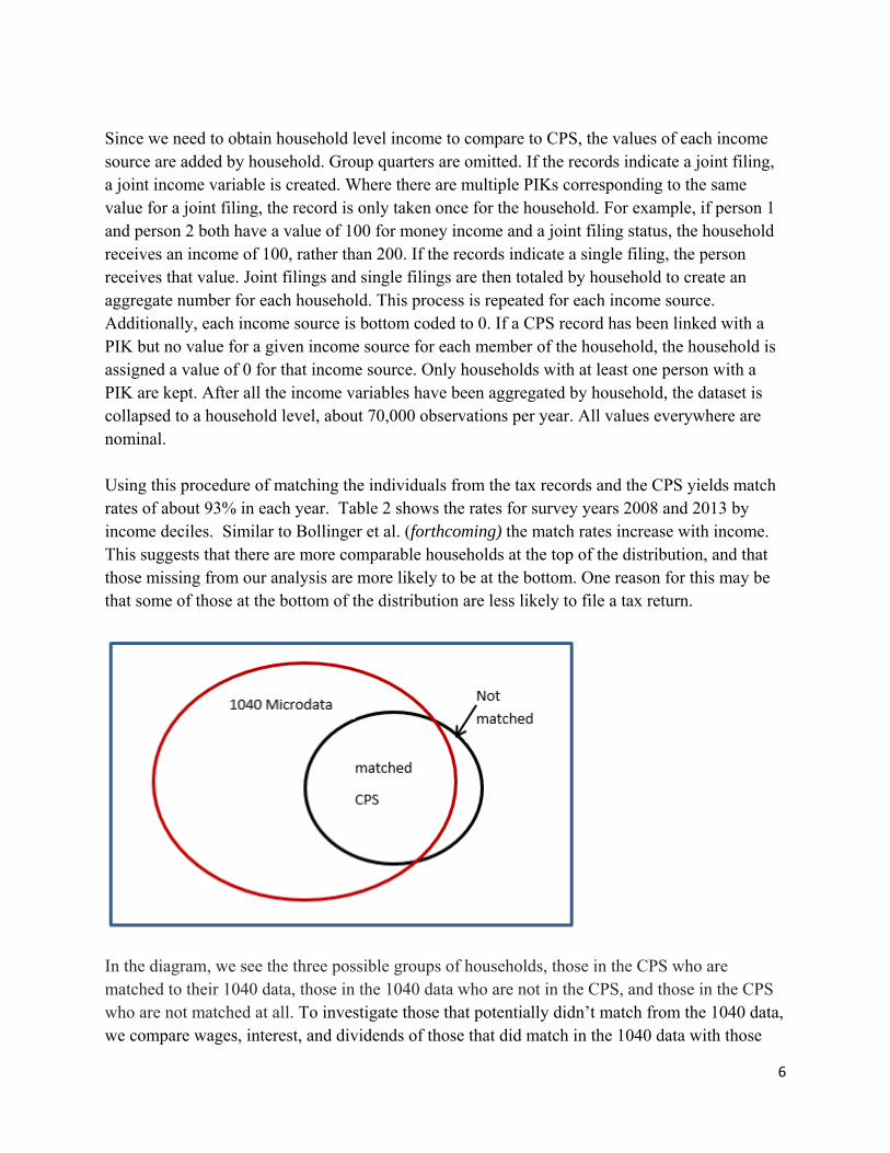
In the diagram, we see the three possible groups of households, those in the CPS who are matched to their 1040 data, those in the 1040 data who are not in the CPS, and those in the CPS who are not matched at all. To investigate those that potentially didn’t match from the 1040 data, we compare wages, interest, and dividends of those that did match in the 1040 data with those

7  

that did not (i.e. those inside the red circle). For each of the income sources above, we constructed a factor by income source category (see more detail in next section) based on the comparison of the means. For example, if the mean of 1040 wages for those with wages greater than 1m was 2,507,000 for the unmatched and 2,195,000 for the matched, that would mean a factor of 2,507,000/2,195,000 = 1.14.

For the internal, unmerged CPS, the data is processed by aggregating up to a household level. Wages, interest, and dividends are individually bottom-coded to 0. Next, wages, interest, and dividends are multiplied by the “factors” (described above), in the following way: Wages are scaled if they are 1m+. Interest and Dividends are scaled if they are 100k+. Similar to FJFC, we compare a “money income” value, which is census money income (bottom-coded to 0) with a “scaled money income” value, which replaces the values for wages, interest, and dividends with their new values (multiplied by the factors), while keeping the other components of money income intact.7 In the next section, we will explore how the distributional properties of this new distribution differ from the internal CPS. Results To begin our discussion, we first assess the differences between the CPS and the 1040 microdata by constructing a variety of comparisons in order to ascertain the usefulness of using administrative data to enhance survey data results. One of the key results is that there are major differences between what households report to the CPS and provide to the IRS. While some of these differences could be due to a match that is not accurate, given the high match rates, much of the difference is due to under- or over-reporting on the CPS. Recalling the diagram above, in Figures 2 and 3), we compare the reported incomes for 2012 in the CPS and matched incomes for 2012 in the 1040 of those in the overlapping black and red circles. Figure 2 compares the distribution for the tax money income variable to the Census money income. Both income variables are bottom coded to 0. While the frequencies look similar, there are many more zeros in the tax data. If we remove the zeros (the first income category), the distributions are much closer. The distribution of the tax income variable is more left skewed, with more lower income values. However, for the top cells, there are more tax income values than Census income values. Figure 3 shows the means by income category. We note that the maximum number of tax money income is substantially larger than CPS, though the distributions are otherwise comparable. Figures 2A and 3A shows the same graphs for wages. The comparable results demonstrate that the discrepancy is not driven by other income sources.

                                                            7 In FJFC a concept of “pseudo money income” was used. That concept included the subtraction of income variables that were not a part of PI.

8  

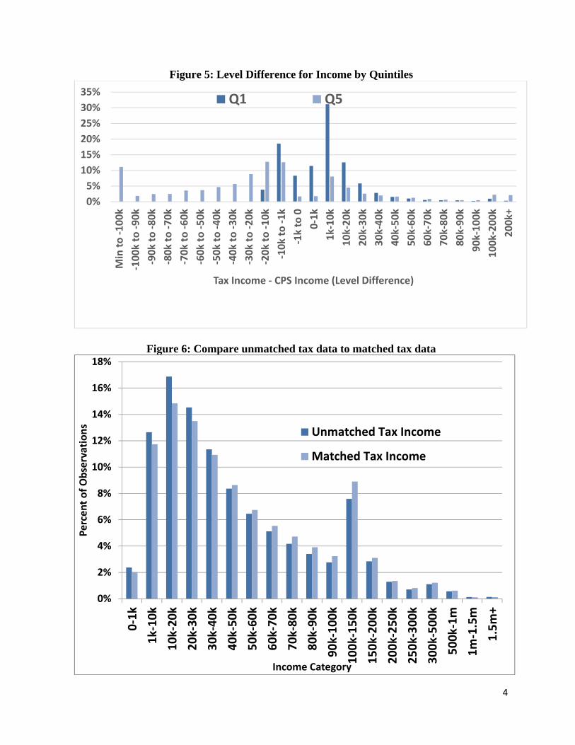
Figure 4 shows the level difference for each household of “constructed income”, defined as the sum of the comparable income components (wages, interest, dividends, and social security) from both CPS and tax data for 2012. The difference is the tax income value less the comparable CPS value. Any households where the constructed income value was 0 were considered missing. If we compare wages instead in Figure 4A, we see the same pattern. The implicit assumption in studies of income distribution is that the measured income in surveys can be improved by using tax data; the idea being that there are penalties for misreporting income on tax forms. However, as these figures demonstrate, there are large differences between the CPS reports and the IRS reports for the same income for the same household and the differences are not uniformly of one sign. The discrepancy is striking and violates a prior hypothesis that CPS income is consistently underreported. There is a substantial frequency of both positive and negative differences occurring at both the top and bottom end of the distributions.8 Figure 4 shows that two-thirds of the households have a difference in incomes less than 20,000 in either direction. However, there are some large differences – 5% have values more different than 100,000. Figure 4A isolates the comparison to earnings (salaries and wages). Turek et al. (2012) also find large differences between the administrative earnings data (DER) and the CPS earnings data, which are similarly distributed on both sides (i.e., CPS>DER and DER>CPS). We could hypothesize that looking at differences overall masks systematic differences at either end of the distribution. It could be supposed that CPS incomes are higher than tax incomes at the lower end and lower at the upper end. However, this is not the case. Figure 5 shows the same differences for 2012, but for the lowest quintile and highest quintile respectively. These show that it is not always the case that the CPS income is higher than tax income at the low end and lower than tax income at the high end. In the bottom quintile, only 30% of households have CPS income greater than tax income. For those in the top quintile, only 30% have tax income greater than in the CPS. In fact, there are a substantial number of households whose CPS is much higher than their tax income. These relationships hold for wages as well. This demonstrates that one cannot simply replace the CPS income with the tax income. Accordingly, we return to our earlier discussion of those “missing” from the CPS. By comparing tax units that merged with the CPS with those that didn’t and considering their respective income distributions, we can determine whether the CPS sample is missing people (and households) at the top of the distribution. Figure 6 shows the distribution comparison. Similar to the CPS and tax income comparison (Figure 2), the non-matched has more lower income values. This is due to the lower match rates at the lower income levels. At the high income categories, there are more matched than non-matched, except for to top two categories. Hence, the main differnces

                                                            8 It is important to keep in mind that the difference is for matched files and does not bear on the use of tax data to improve the representability of the upper part of the distribution.

9  

are at the very top of the distribution. The non-matched show 0.31% over 1M, while the matched have only 0.18%. In addition, the mean income for the top category (over 1.5M) is 50% higher for the non-matched than the matched households. Together, these results suggest that the CPS does not capture the very top of the distribution. This is similar to Burkhauser et al. (2012). While Bee et al. (2015) suggest that there are not differences in response rates for the high end of the distribution, they did not examine households within the top 5%. As described in the methodology section, we can use these results to create factors, which are constructed using the ratio of the mean of the not-matched tax data/tax data matched to CPS for each income category. In this sense, we can obtain a picture of the different samples. Obviously the unmatched sample is very large. However, if the income distribution is different that could suggest that the CPS may have some under-reporting or missing observations when compared to the universe of the 1040 microdata. Table 3 shows the resulting factors for 2012.9 As we can see, the distributions of unmatched and matched tax data are very similar. The factors are significantly different from one in the lowest income category (as we discussed earlier) and in the highest for each factor. Given that there are no households with extremely large interest or dividends in the CPS, the factors are only applied to interest and dividend incomes greater than 100K. For wages, the factor of 1.14 is applied to incomes greater than 1M.

As described in the methodology section, once top wages, interest, and dividends have been multiplied by the factors above, total money income is recalculated ("scaled money income"). Tables 4 and 5 show the impacts on distributional measures for money income (internal cps) and scaled money income. The adjustments for top incomes slightly increases all three measures in Table 4– Gini, share of top 1% and share of top 5%. These adjustments also affect the change in the trends for incomes earned in 2007 and 2012, showing increasing inequality. Table 5 breaks the distribution into (weighted) quintiles.10 Though, in real terms, mean income declined for all quintiles, it declined least for the top quintile, which is also the only quintile affected by this methodology.

An alternative method to create factors could be by ranking the distributions by total income. We found that there was so much re-ranking that the results depended on whether the distribution was ranked using CPS money income or tax income. Ranking by tax income and determining the ratio of tax income to CPS income yielded factors that were greater than one only in the top decile, with a factor of about 2 for the top percentile. However, tax income was below CPS income for the bottom 9 deciles. As a result, inequality would be increased, but it is                                                             9 They are nearly identical for 2007. 10 It does not matter whether the quintiles are reconstructed or not for scaled money income because all the action is within the top 10% essentially, so they do not change. 

10  

not clear that these over-reports of income in the CPS should be ignored. Hokayem, et al. (2015) find the same results using wages from the detailed earnings records (DER) at SSA, which are basically the W-2 records that appear in the 1040. They develop a complicated imputation method to use both the CPS and DER information. Fixler and Johnson (2014) compared AGI in the CPS to the 1040 Microdata and found that the ratio between tax income and the CPS was also less than one until the 80th percentile (see Figure 8.5). They attempted to use the SOI aggregate data to adjust the CPS for top incomes. Again, because of the fact that the tax record data was lower than the CPS at the low income levels, the impact on inequality – both level and trend – was not significant. Accordingly, with the results analyzed in this section, our next step is to use the new adjusted micro data to compute the other categories in personal income. This method would follow FJFC and use both CPS and CE incomes to impute the income components. With the top adjusted wages, interest and dividends, however, this should increase the shares at the top and bring our results closer to those in PSZ. As an example of this process, we consider the interest and imputed interest.

Adding Personal Income Imputed Interest to the distribution of Money Income

In moving from Census Money Income to Personal Income, the single largest component to add is imputed interest (See FJFC, Table 2). The category contains the imputed interest from financial institutions, insurance companies and owner occupied rent. The main hurdle is adjusting the CPS distribution so that the upper tail is more representative; as established above we know that the CPS is missing households at the upper end of the distribution.

More specifically, in the public use file, which we use for this step of the analysis, the small sample sizes in the CPS for the top two income brackets, 1.5m-2m and 2m+, lead to small sample weights and thus underreported population counts for these brackets. The SCF is known for over-sampling high income families, which leads to more representative population totals in the top tail of the distribution. For this analysis we adjust the weights in the CPS by taking the ratio of the SCF and CPS population totals for the top two income brackets. This ratio was multiplied by the CPS population total, in effect giving the SCF population. This new population total was divided by the CPS sample size for the two brackets to create a new household weight. Each household in the bracket then had the CPS weight replaced by the new adjusted weight. As a result, the number of households in the CPS population total increases by the difference of the sum of the top two bracket population totals for the SCF and CPS. As Figure 7 illustrates, in 2012 the CPS population totals for the 1.5m-2m and 2m+ brackets were 12,906 and 6,861 respectively and the overall population total was 122,459,424. The SCF population totals for the 1.5m-2m and 2m+ brackets were 79,145 and 187,528 respectively with an overall population total of 122,530,070. After we adjust the CPS weights to match those of the SCF, the overall population total for the CPS increases by (79,145 + 187,528) – (12,906 + 6,861) = 246,906. The new overall CPS population is therefore 122,459,424 + 246,906 = 122,706,330.

11  

To allocate the PI imputed interest total, we use information from the CPS, SOI and SCF to determine the shares of income that come from interest. Those shares are based on nominal interest from financial instruments—bank accounts and bonds. We compute the interest income shares from each series in each income category, take the arithmetic mean and then use the mean to allocate the total imputed interest. Table 6 shows the distribution of interest income in the various surveys. The second column from the right shows that amount of imputed interest in PI and the far-right column shows the amount allocated to each household. For example, in 2012 imputed interest in PI is 598 billion dollars, and each household in the highest income category receives about 478,000 dollars.

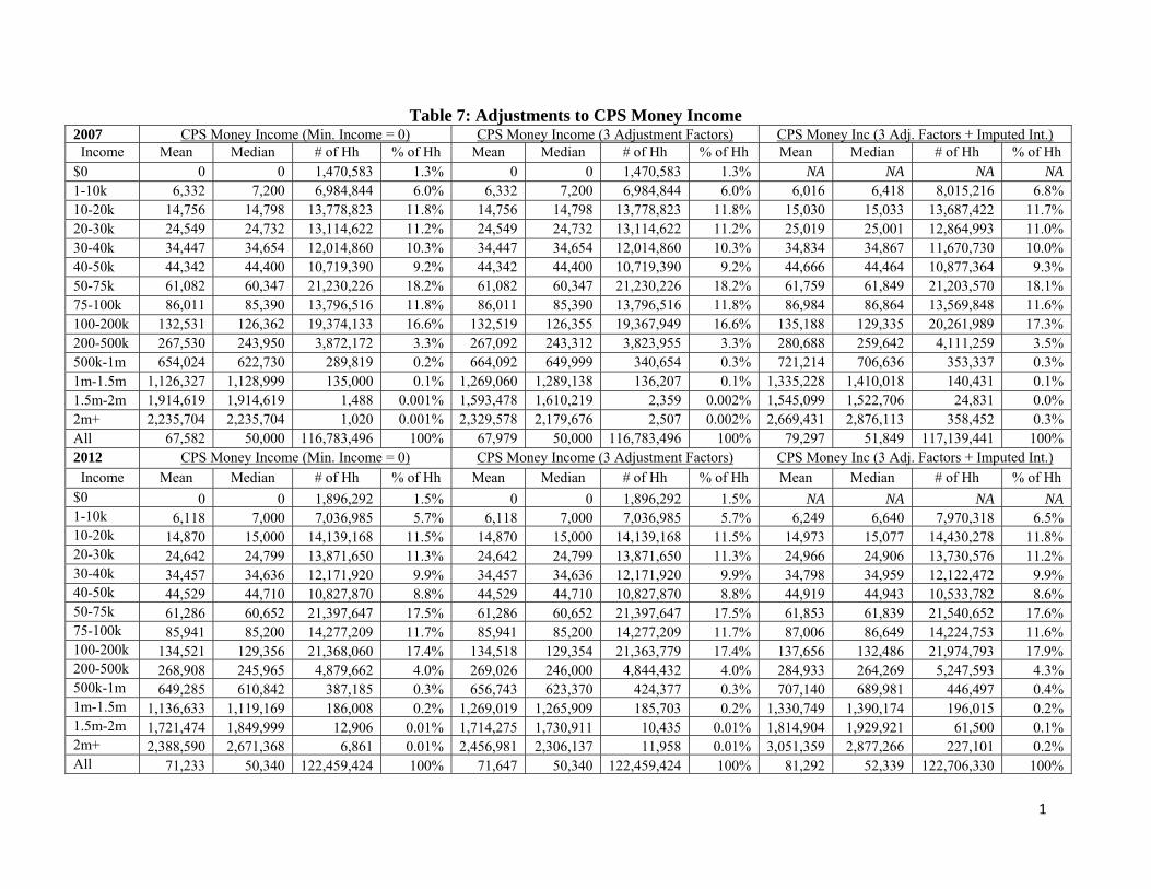
Table 7 shows the impact of several adjustments. To begin we set the minimum CPS money income level equal to zero—the corresponding distribution is given in the far-left section of the table in each panel. The middle section shows the impact on CPS money income of applying the three factors discussed above. The impact is not great and essentially leaves the values for the upper tail unchanged. The far-right section shows the impact on the factor adjusted money income by the addition of imputed interest. The percent of households in the upper tail has gone up by an order of magnitude.

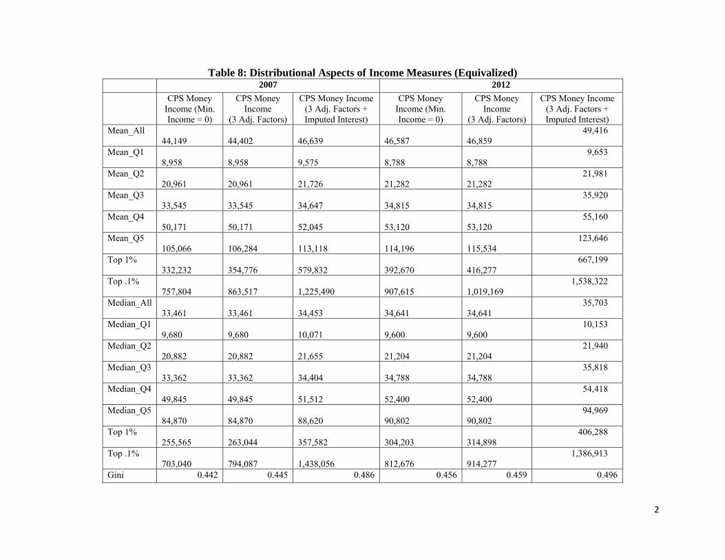
Table 8 presents the distributional aspects of the income measures presented in Table 7, except that in Table 8 the incomes are equivalized.11 Some notable features of the table are: the addition of imputed interest greatly affects the means and medians at the upper tail; for all the categories, the mean is less than the median except for the top 0.1%; the means and medians within the top quintile are hugely different; and correspondingly the Gini coefficients increase.

Conclusion

This paper is part of a project to create a distribution for the US national account concept of Personal Income. We focus on two topics. First, we examine whether the substitution of Federal income tax data improves the survey-based measures of money income in the CPS. We find that the impact of this substitution is marginal; the differences between the money income using tax data and the collected money income is almost equally likely to be either positive or negative. Because this result focuses on the matched files in the CPS and the tax data, we turn to looking at the information in the unmatched tax data. More specifically we look at the ratio of unmatched to matched for three sources of income: wages, dividends and interest. We use these ratios (factors) to adjust the distribution of the money income for the upper tail—the part of the distribution for which the ratio only mattered—and find that again the change is marginal. This leads to the conclusion that there is not much to gain by matching the survey-based money income with the tax data. We did, however, confirm the well-known result that the CPS is not representative for the upper tail of the income distribution.

Second, using the factor-adjusted money income we moved toward the Personal Income measure                                                             11 Equivalization is done by dividing income by the square root of the number of members of the household. 

12  

by including imputed interest—the largest source of a difference between Personal Income and money income. Recognizing that imputed interest is likely more important at the upper tail, we first adjusted the upper tail of the CPS distribution using information in the SCF. We then determined a distribution of interest income and then allocated imputed interest accordingly. We find that the addition of imputed greatly affects the upper tail—the mean and median for the top quintile is below that of the top 1% and 0.1% and the mean and medial for the former are substantially less than those of the former. We then show that as expected the Gini rises.

13  

References: Abowd, J. and M.H. Stinson. “Estimating Measurement Error in Annual Job

Earnings: A Comparison of Survey and Administrative Data.” Review of Economics and Statistics, 95: 1451-1467, 2013

Atkinson, A., Piketty, T. and E. Saez, “Top Incomes in the Long Run of History", Journal of Economic Literature, 49:1, pp 3-71, 2011.

 Bee, C. A, Gathright, G. and B. D. Meyer. “Bias from Unit Non-Response in

the Measurement of Income in Household Surveys,” Unpublished Paper, August 2015. Bee, A., and J. Mitchell. "Do Older Americans Have More Income Than We Think?" SESHD

Working Paper #2017-39. July 2017 Bollinger, C., Hirsch, B., Hokayem, C., and J. Ziliak, “Trouble in the Tails? What We Know

about Earnings Nonresponse Thirty Years after Lillard, Smith, and Welch,” forthcoming in Journal of Political Economy.

Boushey, H. and A. Clemens, “Disaggregating growth: Who prospers when the economy grows”

Washington Center for Equitable Growth Equitable Growth March 2018 Boushey, H. and A. Hersh, The American Middle Class, Income Inequality, and the Strength of

Our Economy New Evidence in Economics, Center for American Progress report, May 2012.

Boushey, H. and C. Price, “How are Economic Inequality and Growth Connected?,” Washington Center for Equitable Growth, October 2014.

Burkhauser, R.V., Feng, S. Jenkins, S. and J. Larrimore. “Recent Trends in Top Income Shares

in the USA: Reconciling Estimates from March CPS and IRS Tax Return Data.” Review of Economics and Statistics, 94 (2): 371-388. 2012

Burkhauser, R., Herault, N., Jenkins, S. and R. Wilkins, “Top incomes and inequality in the UK:

reconciling estimates from household survey and tax return data,” Oxford Economic Papers, Oxford Economic Papers, 70(2), 2018, 301–326, 2017

Burkhauser, R., J. Larrimore, J. and K. Simon, “A "Second Opinion" On The Economic Health Of The American Middle Class” NBER Working Paper 17164, 2012.

Congressional Budget Office, “The Distribution of Household Income and Federal Taxes, 2014,

CBO report, 2018.

Council of Economic Advisors, Economic Report of the President, 2015, GPO, 2015.

14  

Cynamon, B.Z and S.M. Fazzari, “Household Income, Demand, and Saving: Deriving Macro

Data with Micro Data Concepts,” Review of Income and Wealth, May 2015.

DeNavas-Walt, C. and B. D. Proctor, Income and Poverty in the United States: 2013, U.S. Census Bureau, Current Population Reports, P60-249, U.S. Government Printing Office, Washington, DC, 2014.

Fesseau, M., and M-L. Mattonetti, “Distributional Measures across Household Groups in a National Accounts Framework,” Working Paper n°53, Paris: OECD. 2013.

Fisher, J., Johnson, D. and T. Smeeding, “Inequality of Income and Consumption: Measuring the Trends in Inequality from 1984–2011 for the Same Individuals,” Review of Income and Wealth, online release, 2014

Fisher, J., Johnson, D. Thompson, J. and T Smeeding, “Inequality in 3D: Income, Consumption

and Wealth, NBER presentation, July 2015.

Fitzwilliams, J.M., “Size Distribution of Income in 1963,” Survey of Current Business, Vol. 44, No. 4, April 1964.

Fixler, D. and D. Johnson, “Accounting for the Distribution of Income in the US National Accounts” in Measuring Economic Stability and Progress, D. Jorgenson, J. S.Landefeld, and P. Schreyer, editors, Chicago: University of Chicago Press, 2014.

Fixler, D., Johnson, D., Furlong, K. and Craig, A. “A Consistent Data Series to Evaluate Growth and Inequality in the National Accounts,” Review of Income and Wealth, forthcoming.

Goldsmith, S., “Income Distribution in the United States, 1950-53,” Survey of Current Business, March 1955.

Goldsmith, S., “The Relation of Census Income Distribution Statistics to Other Income Data,” in An Appraisal of the 1950 Census Income Data, CRIW ed, NBER, 1958.

Haig, R. M., "The Concept of Income—Economic and Legal Aspects". The Federal Income Tax. New York: Columbia University Press. pp. 1–28, 1921.

Hokayem, C., Bollinger, C. and J. Ziliak. “The Role of CPS Nonresponse in the Measurement of

Poverty,” Journal of the American Statistical Association 110 (511): 935-045.2015. Irwin, N., “You Can’t Feed a Family with GDP,” New York Times, Sept 16, 2014.

Jenkins, S. “Pareto Models, Top Incomes, and Recent Trends in UK Income Inequality”,

Economica, 84, pp. 261-289, 2017

15  

Jorgenson, D. W., “Aggregate Consumer Behavior and the Measurement of Social Welfare,” Econometrica, 58:5, pp. 1007-1040, 1990.

Jorgenson, D. W. and P. Schreyer, “Measuring Individual Economic Well-Being and Social

Welfare within the Framework of the System of National Accounts,” OECD/IARIW Conference paper, 2015.

Kuznets, S., “Economic Growth and Income Inequality,” The American Economic Review, Vol.

45, No. 1, pp. 1-28, 1955

McCully, C., “Integration of Micro and Macro Data on Consumer Income and Expenditures,” in Measuring Economic Stability and Progess, D. Jorgenson, J. S.Landefeld, and P. Schreyer, editors, Chicago: University of Chicago Press, 2014.

OECD, Divided We Stand: Why Inequality Keeps Rising, OECD Publishing, 2011. OECD, “Reducing Income inequality while boosting economic growth: Can it be done?” in

Economic Policy Reforms 2012, OECD, 2012. OECD, "Focus on Inequality and Growth - December 2014.” Online access

www.oecd.org/social/inequality-and-poverty.htm , 2014. OECD, Handbook on compiling distributional results on household income, consumption and

saving consistent with national accounts, 2016 Office of Business Economics, Income Distribution in the United States by Size, 1944-1950,

Washington: U.S. GPO, 1953. Office of National Statistics (ONS) (2016) “Effects of taxes & benefits on household income:

Methodology & Coherence 2014/15.” London: Office for National Statistics ONS (2016).

Piketty, T., Capital in the Twenty-First Century, Cambridge: Harvard University Press, 2014.

Piketty, T. and E. Saez, "Income Inequality in the United States, 1913-1998," Quarterly Journal of Economics, 118(1), 1-39, 2003.

Piketty, T., E. Saez, and G. Zucman, “Distributional National Accounts: Methods and Estimates for the United States since 1913,” Quarterly Journal of Economics,113(2), 553-609, 2018.

Roemer, Mark. “Using Administrative Earnings Records to Assess Wage Data Quality in the

Current Population Survey and the Survey of Income and Program Participation.” Longitudinal Employer Household Dynamics Program Technical Paper No. TP-2002-22, US Census Bureau, 2002.

Rothbaum, J. “Comparing Income Aggregates: How do the CPS and ACS Match the National Income and Product Accounts, 2007-2012”, SEHSD Working Paper 2015-01, January 2015.

16  

Ruggles, N. and R. Ruggles, “A Strategy for Merging and Matching Microdata Sets.” Annals of

Economic and Social Measurement 3: 353-371, 1974 Sabelhaus, J., Johnson, D., Ash, S.,Swanson, D., Garner, T., Greenlees, J. and S. Henderson, “Is

the Consumer Expenditure Survey Representative by Income?” in Improving the Measurment of Consumer Expenditures, C. Carroll, C., T. Crossley, and J. Sabelhaus, editors, University of Chicago Press, 2015.

Smith, C. “What’s the matter with GDP?” Financial Times, 26 July 2018.

Simons, H., Personal Income Taxation: the Definition of Income as a Problem of Fiscal Policy. Chicago: University of Chicago Press, 1938.

Stiglitz, J.E., A. Sen, and J. Fitoussi, Report by the Commission on the Measurement of Economic Performance and Social Progress. United Nations Press, 2009

Turek, J., Swenson, K. Ghose, B. Scheuren, F. and D. Lee, “How Good Are ASEC Earnings Data? A Comparison to SSA Detailed Earning Records” (2012)  

Yellen, J., “Perspectives on Inequality and Opportunity from the Survey of Consumer Finances,” Remarks at the Conference on Economic Opportunity and Inequality, Federal Reserve Bank of Boston, 2014.

17  

Tables and Figures Table 1: Comparison of Income concepts

SOURCE Haig/ Simons

Census PI/NIPA (BEA)

CBO SOI (AGI)

Canberra

Employment income Yes Yes Yes Yes Yes Yes Employer contribution to Soc Sec Yes No Yes Yes No Yes Employer-provided benefitsa Yes No Yes Yes No Yes Investment income Yes Yes Yes . Yes Yes Yes Imputed investment income Yes No Yes No No No Government cash transfers Yes Yes Yes Yes Yes

(taxable) Yes

Employee contribution to Soc Sec Yes Yes No (subtract)

Yes Yes Yes

Retirement income Yes Yes No (only int.)

Yes Yes Yes

Cash assistance from others Yes Yes No Yes No Yes Realized capital gains Yes No No Yes Yes No Lump sum (IRA disbursements) Yes No No Yes Taxable Yes In-kind government transfersa Yes No Yes Yes No Nob Other In-kind transfersa Yes No No No No Nob Home production Yes No No No No In concept Imputed renta Yes No Yes No No Yes Unrealized capital gains Yes No No No No No Savings withdrawals Yesc No No No No No a Estimates are imputed in the CPS b included in the final measure of disposable income c included in the Haig-Simons equation; depletions in savings will simply increase consumption

Table 2: Linkage Rates of CPS ASEC to tax data by Money Income Decile

Linked Rate 2007 2012 Decile 1 86.4% 86.3% Decile 2 89.3% 90.1% Decile 3 90.3% 90.9% Decile 4 91.7% 92.0% Decile 5 92.2% 92.3% Decile 6 93.1% 92.8% Decile 7 93.4% 93.6% Decile 8 94.7% 93.6% Decile 9 95.0% 94.6% Decile 10 94.8% 94.3% Overall 92.9% 92.5%

18  

Table 3: Tax Data Unmatched-Matched Factors (2012) Wages Interest Dividends

0-1k 0.846 0-1k 0.991 0-1k 0.947 1k-10k 1.022 1k-10k 1.015 1k-10k 1.024 10k-20k 1.000 10k-20k 0.978 10k-20k 1.003 20k-30k 0.997 20k-30k 0.992 20k-30k 0.998 30k-40k 0.999 30k-40k 0.994 30k-40k 0.997 40k-50k 0.999 40k-50k 1.005 40k-50k 0.994 50k-60k 0.999 50k-60k 0.984 50k-60k 1.001 60k-70k 0.999 60k-70k 1.002 60k-70k 0.999 70k-80k 1.001 70k-80k 1.002 70k-80k 1.010 80k-90k 1.000 80k-90k 1.010 80k-90k * 90k-100k 1.000 90k-100k 1.008 90k-100k * 100k-150k 1.003 100k-150k 1.010 100k-150k 1.021 150k-200k 1.001 150k+ 2.940 150k+ 1.377 200k-250k 0.997 250k-300k 0.998 300k-500k 1.005 500k-1m 0.998 1m+ 1.142

               * indicates there were too few observations to report this factor  

Table 4: Scaled vs. Unscaled Distribution Results

2007 2012 2007-2012 Unscaled Scaled Unscaled Scaled %Δ Unscaled %Δ Scaled Top 1% Share 0.122 0.124 0.130 0.136 7.2% 8.9% Top 5% Share 0.238 0.240 0.249 0.254 4.8% 5.7% Gini 0.463 0.465 0.477 0.480 3.1% 3.4% N 76,000 76,000 75,000 75,000

 

Table 5: Scaled vs. Unscaled Quintiles

2007 2012 (deflated) 2007-2012 (deflated) Quintile Unscaled Scaled Unscaled Scaled %Δ Unscaled %Δ Scaled 0-20% 11560 11560 10150 10150 -12.2% -12.2% 20-40% 29450 29450 26191 26191 -11.1% -11.1% 40-60% 49980 49980 45133 45133 -9.7% -9.7% 60-80% 79210 79210 72400 72400 -8.6% -8.6% 80-100% 168300 169300 160410 162350 -4.7% -4.1%

Table 6: A Comparison of Interest Distributions by Income Bracket 2007 CPS SCF SOI Arith.

Mean of Share

Imputed Interest

(Billions)

Allocated Impt. Int.

Value Income Bracket

Population Amount (M)

Share Population Amount (M)

Share Population Amount (M)

Share

$0 1,470,583 4.1 0.0% 473,934 1,484.4 0.8% 1,907,835 9,179.0 2.6% 1.1% 5.5 3,767 1-10k 6,984,844 675.8 0.3% 7,351,360 263.7 0.1% 24,045,493 4,785.7 1.4% 0.6% 2.9 418 10-20k 13,778,823 3,330.5 1.4% 15,422,830 1,566.0 0.8% 22,976,467 11,038.8 3.2% 1.8% 8.7 633 20-30k 13,114,622 6,456.6 2.7% 15,147,642 4,270.0 2.2% 18,969,031 10,710.6 3.1% 2.6% 12.9 985 30-40k 12,014,860 8,058.9 3.3% 13,270,849 4,447.4 2.3% 14,740,806 11,301.9 3.3% 2.9% 14.4 1,201 40-50k 10,719,390 9,099.7 3.8% 10,774,324 3,356.0 1.7% 11,150,798 10,536.5 3.0% 2.8% 13.9 1,294 50-75k 21,230,226 25,055.8 10.4% 20,126,294 10,135.3 5.1% 19,450,744 29,710.3 8.6% 8.0% 39.3 1,849 75-100k 13,796,516 27,475.1 11.4% 12,023,315 13,300.3 6.8% 11,744,132 26,427.3 7.6% 8.6% 42.0 3,042 100-200k 19,374,133 96,533.6 40.0% 15,553,917 29,636.5 15.1% 13,457,876 54,275.5 15.6% 23.5% 115.2 5,945 200-500k 3,872,172 57,144.3 23.7% 4,343,757 32,199.6 16.4% 3,492,353 47,803.1 13.8% 17.9% 87.7 22,642 500k-1m 289,819 5,858.0 2.4% 959,512 23,755.7 12.1% 651,049 25,865.2 7.4% 7.3% 35.8 123,392 1m-1.5m 135,000 1,695.1 0.7% 301,455 16,037.8 8.1% 166,362 13,516.1 3.9% 4.2% 20.8 153,819 1.5m-2m 126,615* 59.5 0.0% 126,615 12,112.3 6.2% 70,733 8,577.9 2.5% 2.9% 14.1 111,313 2m+ 231,837** 32.9 0.0% 231,837 44,350.2 22.5% 155,125 83,681.8 24.1% 15.5% 76.0 327,868 Total 117,139,441 241,480.1

116,107,641 196,915.1 142,978,804 347,409.5 100.0% 489.1

2012 CPS SCF SOI Arith. Mean of

Share

Imputed Interest

(Billions)

Allocated Impt. Int.

Value Income Bracket

Population Amount (M)

Share Population Amount (M)

Share Population Amount (M)

Share

$0 1,896,292 15.0 0.0% 434,777 3,392.5 2.2% 2,128,548 7.8 4.3% 2.2% 12.6 6,640 1-10k 7,036,985 536.5 0.4% 5,383,875 289.7 0.2% 22,336,318 2.8 1.6% 0.7% 4.1 577 10-20k 14,139,168 1,838.2 1.2% 17,628,149 1,508.6 1.0% 24,247,770 5.0 2.7% 1.6% 9.6 678 20-30k 13,871,650 3,218.7 2.1% 16,046,110 2,075.9 1.3% 18,903,110 5.0 2.7% 2.1% 12.1 870 30-40k 12,171,920 4,230.5 2.8% 14,675,884 1,683.8 1.1% 14,451,152 4.7 2.5% 2.2% 12.5 1,028 40-50k 10,827,870 5,273.1 3.5% 11,566,124 1,870.4 1.2% 10,873,672 5.2 2.9% 2.5% 14.7 1,357 50-75k 21,397,647 15,546.9 10.4% 19,894,966 4,459.1 2.9% 18,985,371 12.9 7.0% 6.8% 39.3 1,839 75-100k 14,277,209 16,673.7 11.1% 12,314,149 6,441.2 4.2% 12,103,891 11.5 6.3% 7.2% 41.8 2,929 100-200k 21,368,060 58,739.8 39.2% 17,238,928 24,711.4 16.1% 15,646,648 26.8 14.6% 23.3% 135.4 6,336 200-500k 4,879,662 39,071.9 26.1% 5,435,720 38,515.5 25.0% 4,154,112 26.6 14.6% 21.9% 127.2 26,065 500k-1m 387,185 3,129.1 2.1% 1,248,706 15,598.9 10.1% 705,029 15.8 8.6% 6.9% 40.4 104,251 1m-1.5m 186,008 1,188.3 0.8% 396,009 12,134.0 7.9% 169,413 7.5 4.1% 4.3% 24.7 132,849 1.5m-2m 79,145* 73.7 0.0% 79,145 9,181.9 6.0% 71,874 5.2 2.8% 2.9% 17.1 216,280 2m+ 187,528** 282.3 0.2% 187,528 32,050.8 20.8% 151,563 46.2 25.3% 15.4% 89.7 478,067 Total 122,706,330 149,817.8 122,530,070 153,913.7 144,928,471 182.9 100.0% 581.1

1  

Table 7: Adjustments to CPS Money Income 2007 CPS Money Income (Min. Income = 0) CPS Money Income (3 Adjustment Factors) CPS Money Inc (3 Adj. Factors + Imputed Int.)

Income Mean Median # of Hh % of Hh Mean Median # of Hh % of Hh Mean Median # of Hh % of Hh $0 0 0 1,470,583 1.3% 0 0 1,470,583 1.3% NA NA NA NA 1-10k 6,332 7,200 6,984,844 6.0% 6,332 7,200 6,984,844 6.0% 6,016 6,418 8,015,216 6.8% 10-20k 14,756 14,798 13,778,823 11.8% 14,756 14,798 13,778,823 11.8% 15,030 15,033 13,687,422 11.7% 20-30k 24,549 24,732 13,114,622 11.2% 24,549 24,732 13,114,622 11.2% 25,019 25,001 12,864,993 11.0% 30-40k 34,447 34,654 12,014,860 10.3% 34,447 34,654 12,014,860 10.3% 34,834 34,867 11,670,730 10.0% 40-50k 44,342 44,400 10,719,390 9.2% 44,342 44,400 10,719,390 9.2% 44,666 44,464 10,877,364 9.3% 50-75k 61,082 60,347 21,230,226 18.2% 61,082 60,347 21,230,226 18.2% 61,759 61,849 21,203,570 18.1% 75-100k 86,011 85,390 13,796,516 11.8% 86,011 85,390 13,796,516 11.8% 86,984 86,864 13,569,848 11.6% 100-200k 132,531 126,362 19,374,133 16.6% 132,519 126,355 19,367,949 16.6% 135,188 129,335 20,261,989 17.3% 200-500k 267,530 243,950 3,872,172 3.3% 267,092 243,312 3,823,955 3.3% 280,688 259,642 4,111,259 3.5% 500k-1m 654,024 622,730 289,819 0.2% 664,092 649,999 340,654 0.3% 721,214 706,636 353,337 0.3% 1m-1.5m 1,126,327 1,128,999 135,000 0.1% 1,269,060 1,289,138 136,207 0.1% 1,335,228 1,410,018 140,431 0.1% 1.5m-2m 1,914,619 1,914,619 1,488 0.001% 1,593,478 1,610,219 2,359 0.002% 1,545,099 1,522,706 24,831 0.0% 2m+ 2,235,704 2,235,704 1,020 0.001% 2,329,578 2,179,676 2,507 0.002% 2,669,431 2,876,113 358,452 0.3% All 67,582 50,000 116,783,496 100% 67,979 50,000 116,783,496 100% 79,297 51,849 117,139,441 100% 2012 CPS Money Income (Min. Income = 0) CPS Money Income (3 Adjustment Factors) CPS Money Inc (3 Adj. Factors + Imputed Int.)

Income Mean Median # of Hh % of Hh Mean Median # of Hh % of Hh Mean Median # of Hh % of Hh $0 0 0 1,896,292 1.5% 0 0 1,896,292 1.5% NA NA NA NA 1-10k 6,118 7,000 7,036,985 5.7% 6,118 7,000 7,036,985 5.7% 6,249 6,640 7,970,318 6.5% 10-20k 14,870 15,000 14,139,168 11.5% 14,870 15,000 14,139,168 11.5% 14,973 15,077 14,430,278 11.8% 20-30k 24,642 24,799 13,871,650 11.3% 24,642 24,799 13,871,650 11.3% 24,966 24,906 13,730,576 11.2% 30-40k 34,457 34,636 12,171,920 9.9% 34,457 34,636 12,171,920 9.9% 34,798 34,959 12,122,472 9.9% 40-50k 44,529 44,710 10,827,870 8.8% 44,529 44,710 10,827,870 8.8% 44,919 44,943 10,533,782 8.6% 50-75k 61,286 60,652 21,397,647 17.5% 61,286 60,652 21,397,647 17.5% 61,853 61,839 21,540,652 17.6% 75-100k 85,941 85,200 14,277,209 11.7% 85,941 85,200 14,277,209 11.7% 87,006 86,649 14,224,753 11.6% 100-200k 134,521 129,356 21,368,060 17.4% 134,518 129,354 21,363,779 17.4% 137,656 132,486 21,974,793 17.9% 200-500k 268,908 245,965 4,879,662 4.0% 269,026 246,000 4,844,432 4.0% 284,933 264,269 5,247,593 4.3% 500k-1m 649,285 610,842 387,185 0.3% 656,743 623,370 424,377 0.3% 707,140 689,981 446,497 0.4% 1m-1.5m 1,136,633 1,119,169 186,008 0.2% 1,269,019 1,265,909 185,703 0.2% 1,330,749 1,390,174 196,015 0.2% 1.5m-2m 1,721,474 1,849,999 12,906 0.01% 1,714,275 1,730,911 10,435 0.01% 1,814,904 1,929,921 61,500 0.1% 2m+ 2,388,590 2,671,368 6,861 0.01% 2,456,981 2,306,137 11,958 0.01% 3,051,359 2,877,266 227,101 0.2% All 71,233 50,340 122,459,424 100% 71,647 50,340 122,459,424 100% 81,292 52,339 122,706,330 100%

2  

Table 8: Distributional Aspects of Income Measures (Equivalized) 2007 2012

CPS Money

Income (Min. Income = 0)

CPS Money Income

(3 Adj. Factors)

CPS Money Income (3 Adj. Factors + Imputed Interest)

CPS Money Income (Min. Income = 0)

CPS Money Income

(3 Adj. Factors)

CPS Money Income (3 Adj. Factors + Imputed Interest)

Mean_All 44,149

44,402

46,639

46,587

46,859

49,416

Mean_Q1 8,958

8,958

9,575

8,788

8,788

9,653

Mean_Q2 20,961

20,961

21,726

21,282

21,282

21,981

Mean_Q3 33,545

33,545

34,647

34,815

34,815

35,920

Mean_Q4 50,171

50,171

52,045

53,120

53,120

55,160

Mean_Q5 105,066

106,284

113,118

114,196

115,534

123,646

Top 1% 332,232

354,776

579,832

392,670

416,277

667,199

Top .1% 757,804

863,517

1,225,490

907,615

1,019,169

1,538,322

Median_All 33,461

33,461

34,453

34,641

34,641

35,703

Median_Q1 9,680

9,680

10,071

9,600

9,600

10,153

Median_Q2 20,882

20,882

21,655

21,204

21,204

21,940

Median_Q3 33,362

33,362

34,404

34,788

34,788

35,818

Median_Q4 49,845

49,845

51,512

52,400

52,400

54,418

Median_Q5 84,870

84,870

88,620

90,802

90,802

94,969

Top 1% 255,565

263,044

357,582

304,203

314,898

406,288

Top .1% 703,040

794,087

1,438,056

812,676

914,277

1,386,913

Gini 0.442 0.445 0.486 0.456 0.459 0.496

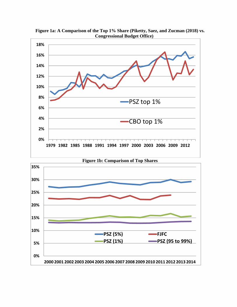
Figure 1a: A Comparison of the Top 1% Share (Piketty, Saez, and Zucman (2018) vs. Congressional Budget Office)

Figure 1b: Comparison of Top Shares

0%

2%

4%

6%

8%

10%

12%

14%

16%

18%

1979 1982 1985 1988 1991 1994 1997 2000 2003 2006 2009 2012

PSZ top 1%

CBO top 1%

0%

5%

10%

15%

20%

25%

30%

35%

20002001 2002 2003 2004 2005 2006 2007 2008 2009 2010 2011 2012 2013 2014

PSZ (5%) FJFC

PSZ (1%) PSZ (95 to 99%)

1  

Figure 2: Comparing CPS Money Income & Tax Money Income

Figure 2A: Comparing CPS Wage & Tax Wage

0%

2%

4%

6%

8%

10%

12%

14%

16%

18%

0‐1k

1k‐10k

10k‐20k

20k‐30k

30k‐40k

40k‐50k

50k‐60k

60k‐70k

70k‐80k

80k‐90k

90k‐100k

100k‐150k

150k‐200k

200k‐250k

250k‐300k

300k‐500k

500k‐1m

1m‐1.5m

1.5m‐2m

2m+

% of Observations

Income Category

Tax Money Income

0%

5%

10%

15%

20%

25%

30%

35%

% of Observations

Wage Category

Tax Wage CPS Wage

2  

Figure 3: Mean Incomes by Income Category (Matched CPS)

Figure 3A: Comparing Means of CPS Wage & Tax Wage

0

1

2

3

4

5

6

7

0‐1k

1k‐10k

10k‐20k

20k‐30k

30k‐40k

40k‐50k

50k‐60k

60k‐70k

70k‐80k

80k‐90k

90k‐100k

100k‐150k

150k‐200k

200k‐250k

250k‐300k

300k‐500k

500k‐1m

1m‐1.5m

1.5m‐2m

2m+

Mean

 Income (millions)

Income Categories

Tax Money Income

CPS Money Income

$0

$1

$1

$2

$2

$3

Mean

 Wage (Millions)

Wage Categories

Tax Wage CPS Wage

3  

Figure 4: Level Difference in Constructed Income (Tax-CPS)

Figure 4A: Level Difference in Wage

0%

5%

10%

15%

20%

25%Percent of Observations

Level Difference in Constructed Income (Tax ‐ CPS)

0%

5%

10%

15%

20%

25%

Percent of Observations

Level Difference in Wage (Tax ‐ CPS)

4  

Figure 5: Level Difference for Income by Quintiles

Figure 6: Compare unmatched tax data to matched tax data

0%

5%

10%

15%

20%

25%

30%

35%

Min to ‐100k

‐100k to ‐90k

‐90k to ‐80k

‐80k to ‐70k

‐70k to ‐60k

‐60k to ‐50k

‐50k to ‐40k

‐40k to ‐30k

‐30k to ‐20k

‐20k to ‐10k

‐10k to ‐1k

‐1k to 0

0‐1k

1k‐10k

10k‐20k

20k‐30k

30k‐40k

40k‐50k

50k‐60k

60k‐70k

70k‐80k

80k‐90k

90k‐100k

100k‐200k

200k+

Tax Income ‐ CPS Income (Level Difference)

Q1 Q5

0%

2%

4%

6%

8%

10%

12%

14%

16%

18%

0‐1k

1k‐10k

10k‐20k

20k‐30k

30k‐40k

40k‐50k

50k‐60k

60k‐70k

70k‐80k

80k‐90k

90k‐100k

100k‐150k

150k‐200k

200k‐250k

250k‐300k

300k‐500k

500k‐1m

1m‐1.5m

1.5m+

Percent of Observations

Income Category

Unmatched Tax Income

Matched Tax Income

5  

Figure 7: CPS Weights and SCF Weights Incorporated in Top 2 Income Categories

 ‐

 50,000

 100,000

 150,000

 200,000

 250,000

2007 2012 2007 2012

$1,500,000 ‐ $2,000,000 Over $2,000,000

Number of Households

 CPS  SCF