preliminary design and analysis for an immersed tube tunnel across
TRANSCRIPT

PRELIMINARY DESIGN AND ANALYSIS FOR AN IMMERSED TUBE TUNNEL
ACROSS THE İZMİR BAY
A Thesis Submitted to The Graduate School of Engineering and Sciences of
İzmir Institute of Technology in Partial Fulfillment of the Requirements for the Degree of
MASTER SCIENCE
in Civil Engineering
by Nisa KARTALTEPE
October 2008
İZMİR


iii
ACKNOWLEDGEMENTS
I would like to express my sincere gratitude to my supervisor Assist. Prof. Dr.
Gürsoy TURAN and my co-supervisor Assoc. Prof. Dr. İsfendiyar EGELİ for their
guidance, supervisions, and support throughout this study. I also would like to special thanks to Asst. Prof. Dr. Engin AKTAŞ, who is the
member of thesis committee, for their contributions to this thesis.
I also would like to thanks to other members of the thesis committee, Asst. Prof.
Dr. Şebnem ELÇİ and Asst. Prof. Dr. Yusuf ERZİN.
I would like to thank to DLH (The State Railways, Ports, Airports Authority)
and KGM (Republic of Turkey General Directorate of Highways) for providing us
technical reports and data.
Thanks to research assistances at IYTE Department of Civil Engineering who
helped me in anyway along this study. Also special thanks to Anıl ÇALIŞKAN and Aslı
BOR for their good friendships and love.
I offer sincere thanks to my husband Barbaros KARTALTEPE for all his
boundless love, continuous support, understanding, and patience. Finally, I would like
to thank my father, my mother and my sisters for all their love, support, and
encouragement.

iv
ABSTRACT
PRELIMINARY DESIGN AND ANALYSIS FOR AN IMMERSED
TUBE TUNNEL ACROSS THE İZMİR BAY
In this study, a preliminary design and analysis of an immersed tube tunnel is
presented. The tube tunnel will connect the two coasts of the İzmir Bay and whereby
will ease the transportation of the city. The reason to suggest an immersed tube tunnel is
due to the shallow water depth (<25 m) and that the soil profile of the İzmir Bay is
made up of silty-sand. Hence, the Bay is appropriate for an immersed tube tunnel.
First, a possible alignment was assigned for the tunnel. The technical, geometric
properties of the tubes were determined, and the detailed drawings of them were made.
The allowable bearing capacity of the seabed was calculated and it was
determined that the soil has not enough capacity to withstand the design load. The
liquefaction risk of the soil was investigated as well, and it was shown that the soil has
high liquefaction potential.
A static analysis of the tunnel was made in Calculix, a finite element program.
The vertical displacement of the tube unit under static loads was calculated to be above
the permissible settlement value. Afterwards, the seismic analysis was made to
investigate stresses developed due to both racking and axial deformation of the tunnel
during an earthquake. It was found that, the max stress due to the racking effect is less
than the compressive strength of the concrete, and max stress due to the axial
deformation is larger than compressive strength of the concrete. The high in the tube
occur, because of the tubes high stiffness. This problem was solved by releasing the
rigid connections in between two tube units. If these connections are made by using
same form of elastomer joints, the deformation will occur in these joints, releasing the
tubes internal stresses.
Considering these drawbacks, ground improvement was recommended for the
seabed and an increased value of the standard penetration of the soil was estimated.
Then, the analyses were repeated and it was found that all drawbacks were eliminated.
As a conclusion, it was decided that if suggested improvements are made in the
seabed soil, the immersed tube tunnel can be constructed across the İzmir Bay.

v
ÖZET
İZMİR KÖRFEZİ İÇİN BATIRMA TÜP TÜNELİN
ÖN TASARIMI VE ANALİZİ
Bu çalışmada, İzmir Körfezi’nin iki yakası arasında ulaşımı rahatlatmak için
önerilen batırma tünelin ön tasarımı ve analizi yapılmıştır. Batırma tünelin seçilmesinin
nedenleri; İzmir Körfezi’nin oldukça sığ su derinliğine(<25m) sahip olması, zeminin
çoğunlukla yumuşak siltli-kum ihtiva etmesi nedeniyle bu geçiş sistemi için uygun
olmasıdır.
Bu sebeple, öncelikle batırma tünelin güzergahı belirlenmiş, ardından tünelin
teknik ve geometrik özellikleri sunularak en-kesit ve boy-kesit çizimleri yapılmıştır.
Zeminin maksimum ve izin verilebilir taşıma gücü hesaplanmış, bunun tünelin
yerleştirilmesi sonrasında zeminde oluşacak basınç değerinin altında olduğu
gösterilmiştir. Mevcut deney neticeleri kullanılarak zeminin sıvılaşma potansiyeli
incelenmiş ve bu riskin yüksek olduğu saptanmıştır.
Tünelin statik analizi sonlu elemanlar programı olan Calculix yardımıyla
yapılmıştır.Tünelin statik yükler altında düşey yer değiştirmesi hesaplanmış ve meydana
gelen oturma değerinin izin verilen sınır değerinin üstünde olduğu belirlenmiştir.
Ardından, tünelin deprem esnasındaki yanal ve eksensel deformasyonundan
dolayı oluşan gerilmeler hesaplanmıştır. Tünelin yanal ötelenmesi nedeniyle oluşan
gerilmeler betonun basınç dayanımının altında olmasına rağmen, eksensel deformasyon
nedeniyle meydana gelen gerilmelerin betonun basınç dayanımının oldukça üstünde
olduğu tespit edilmiştir. Bu sonucun tünel elemanlarının birbirleriyle rijit olarak
bağlanmasından dolayı oluştuğu anlaşılmıştır. Bu sorun her bir tüp ünitesinin arasına
düşük rijitliğe sahip elastomer malzeme yerleştirilerek büyük gerilmelerin elastomer
bağlantı elemanında oluşması sağlanmış, tüplerin üzerindeki gerilmelerin betonun
basınç dayanımının altında kalması sağlanmıştır.
Bütün bu sakıncaları gidermek için tünel zemininde zemin iyileştirme yapılması
gerekliliği belirtilmiş ve önerilen standart penetrasyon değeri hesaplanmıştır.Yeni
standart penetrasyon değerine göre analizler yinelenmiş ve bütün değerlerlerin kabul
edilebilir seviyelere indiği gösterilmiştir.Çalışmanın sonucunda, gerekli iyileştirmeler
yapıldığı takdirde İzmir Körfezi’nin batırma tüp tünel için uygun olduğu saptanmıştır.

vi
TABLE OF CONTENTS
LIST OF FIGURES ........................................................................................................ ix
LIST OF TABLES .......................................................................................................... xii
CHAPTER 1. INTRODUCTION ..................................................................................... 1
1.1. Purpose .................................................................................................... 1
1.2. Advantages of the Immersed Tube Tunnel ............................................. 2
1.2.1. Contribution to the Environment and Economy ............................. 2
1.2.2. Regional Contributions ................................................................... 2
1.3. Scope of This Study ................................................................................ 5
1.4. Possible Crossing Alternatives ............................................................... 6
1.4.1. Bridges ............................................................................................ 6
1.4.2. Underwater Tunnels ........................................................................ 7
1.5. Soil Profile of the İzmir Bay Bottom ...................................................... 8
1.6. Application History of the Immersed Tube Tunnel ................................ 8
CHAPTER 2. PROPERTIES OF PROPOSED İZMİR BAY IMMERSED
TUBE TUNNEL ...................................................................................... 10
2.1. Possible Route of the Immersed Tube Tunnel ...................................... 10
2.2. Geometric Properties of the Tube ......................................................... 12
CHAPTER 3. CURRENT SEABED –SOIL PROPERTIES .......................................... 16
3.1. Allowable Bearing Capacity ................................................................. 16
3.1.1. SPT Results of the İzmir Bay ........................................................ 19
3.1.2. Allowable Bearing Capacity of the Seabed Soil of the
İzmir Bay. ...................................................................................... 22
3.2. Liquefaction Potential of the Seabed Soil. ............................................ 25
3.2.1. Liquefaction Analysis by using Depth and SPT Data
Relationship. .................................................................................. 26
3.2.2. Liquefaction Analysis by using Simplified Procedure. ................. 27
3.2.2.1. Earthquake Induced Shear Stress Ratio (CSR) .................... 28
3.2.2.2. Depth Reduction Factor ....................................................... 29
vii
3.2.2.3. Cyclic Resistance Ratio (CRR) ............................................ 30
CHAPTER 4. STATIC ANALYSIS FOR PRELIMINARY DESIGN ......................... 37
4.1. Estimation of the Modulus Of Subgrade Reaction ............................... 37
4.1.1. Finding the Modulus of Subgrade Reaction from Stress
Strain Modulus, Es (First method) ............................................... 38
4.1.2. Finding the Modulus of Subgrade Reaction from
Allowable Soil Pressure, qa (Second method) .............................. 39
4.1.3. Application of the First and Second Methods in this Study .......... 41
4.1.4. Calculation of the Spring Constants .............................................. 43
4.2. Static Analysis of the Tunnel for Worst Case Scenario ....................... 47
4.2.1. Total Pressure Transferred to the Seabed Soil ............................. 49
CHAPTER 5. SEISMIC ANALYSIS OF THE IMMERSED TUBE TUNNEL ........... 54
5.1. Types of Deformations .......................................................................... 55
5.2. Seismic Analysis Procedures ................................................................ 55
5.2.1. Free-Field Deformation Approaches ............................................. 57
5.2.1.1. Closed Form Solution Method (Simplified
Procedure) ........................................................................ 57
5.2.2. Soil-Structure Interaction Approaches .......................................... 59
5.2.2.1. Dynamic Earth Pressure ................................................... 59
5.2.2.2. Closed Form Solution Method to Calculate Axial
and Bending Stresses ......................................................... 59
5.2.2.3. Numerical Analysis Method to Calculate Axial
and Bending Stresses ......................................................... 62
5.2.2.4. Closed Form Solution Method to Calculate
Racking Deformations ...................................................... 62
5.3. Application of Seismic Design Procedures in This Study .................... 70
5.3.1. Calculation of the Axial and Curvature Deformations of
the Immersed Tube Tunnel due to an Expected Seismic
Wave Action .................................................................................. 70
5.3.1.1. Closed Form Solution Method .......................................... 72
5.3.1.2. Numerical Analysis Method (Finite Element
Method) ............................................................................. 76

viii
5.3.2. Calculation of Racking Deformations and Stresses of the
Immersed Tube Unit due to an Expected Seismic Wave
Action ............................................................................................. 82
5.3.2.1. Simple Frame Analysis Model ......................................... 82
5.3.2.2. Soil-Structure Interaction Approach ................................. 86
5.4. Seismic Design Issues ........................................................................... 88
5.5. Calculation of Longitudinal Movement between Two
Immersed Tube Units During an Earthquake ....................................... 90
CHAPTER 6. GROUND IMPROVEMENT ALONG THE TUNNEL
ALIGNMENT .......................................................................................... 94
6.1. Ground Improvement ............................................................................ 94
6.1.1. Grouting Types .............................................................................. 95
6.2. Encountered Soil Issues of the İzmir Bay ............................................ 99
6.2.1. Which Method should be used? ................................................... 99
6.3. New Situation of the Seabed Soil after Ground Improvement ........... 100
6.3.1. Allowable Bearing Capacity of the Soil after
Ground Improvement .................................................................. 101
6.3.2. Liquefaction Potential of the Soil after Ground
Improvement ............................................................................... 102
6.3.2.1. Liquefaction Analysis by using depth and SPT
Data Relationship ........................................................... 102
6.3.2.2. Liquefaction Analysis by using Simplified
Procedure ......................................................................... 103
6.3.3. Static Analysis after Ground Improvement ................................. 103
6.4. Analysis Results after the Ground Improvement ................................ 104
CHAPTER 7. CONCLUSIONS ................................................................................... 106
REFERENCES ............................................................................................................. 109

ix
LIST OF FIGURES
Figure Page
Figure 2.1. The possible route of the tunnel .................................................................. 11
Figure 2.2. The water depths on the possible route of tunnel ........................................ 11
Figure 2.3. The technical properties of the IBITT ......................................................... 13
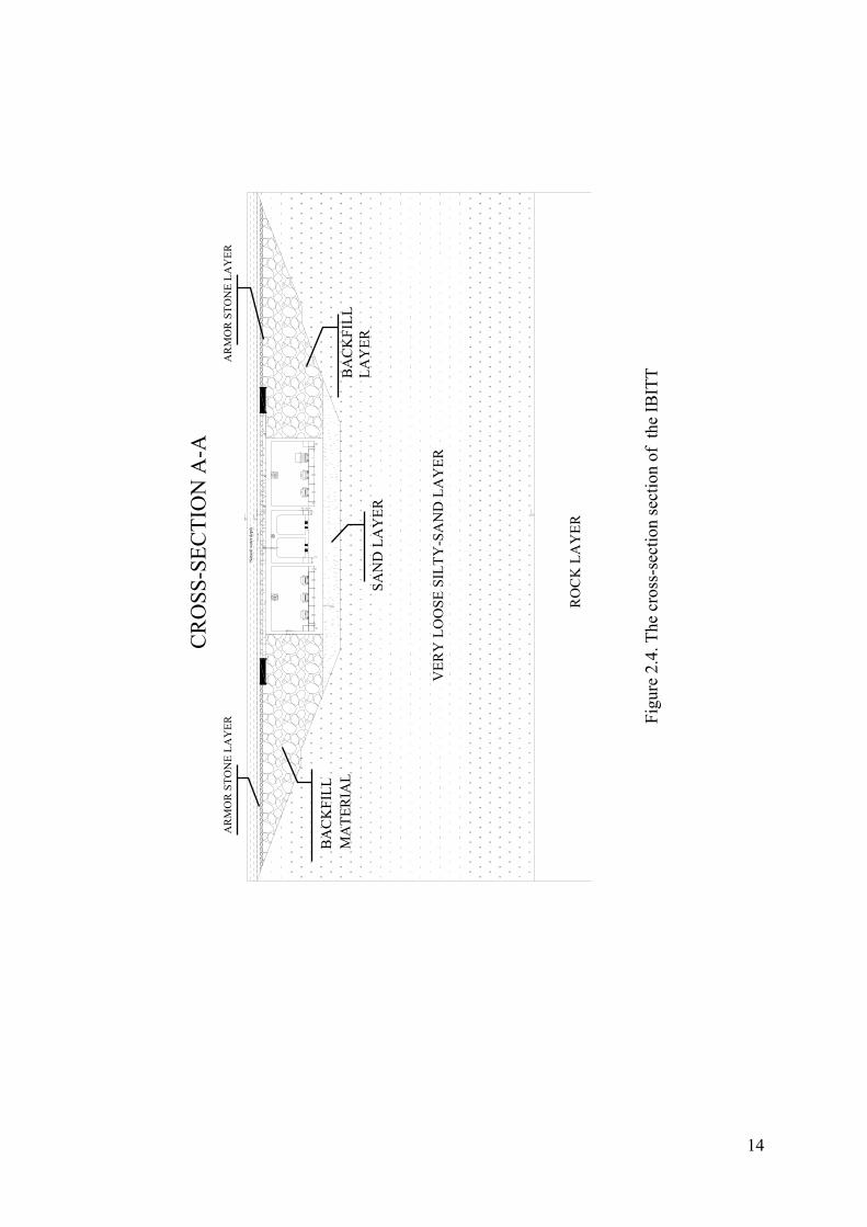
Figure 2.4. The cross-section section of the IBITT ....................................................... 14
Figure 2.5. The longitudinal section of the IBITT ......................................................... 15
Figure3.1. Correction factor for position of water level: (a) depth of water level
with respect to dimension of footing; (b)water level above base of
footing (c): water level below base of footing ............................................. 19
Figure 3.2. The locations of the 3 existing SPT boreholes nearest the IBITT
route ............................................................................................................. 20
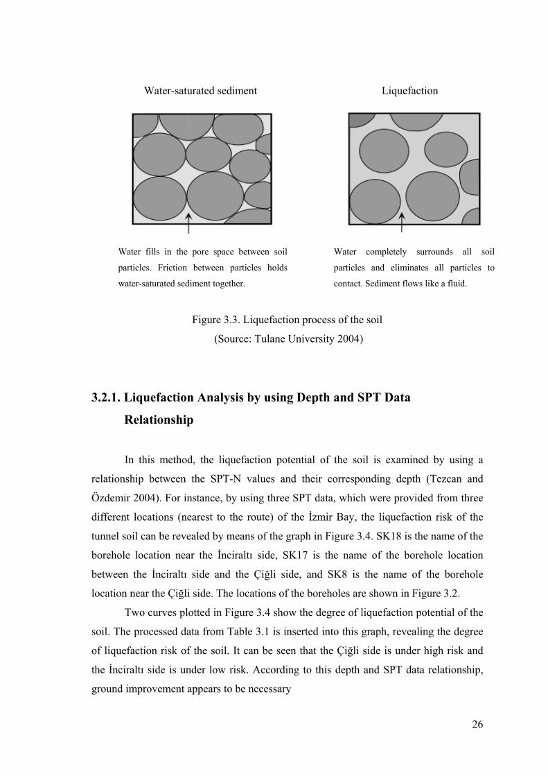
Figure 3.3. Liquefaction process of the soil .................................................................... 26
Figure 3.4. Relationship between the possibility of liquefaction and N values .............. 27
Figure 3.5. Stress ratio and penetration resistance .......................................................... 36
Figure 4.1. Influence factor If for a footing at a depth D ................................................ 39
Figure 4.2. The modeling of the tube unit and the elastic foundation in Calculix ......... 44
Figure 4.3. The weights for vertical spring constants corresponding to each
node of a hexahedral element face ............................................................... 45
Figure 4.4. The modeling of the elastic foundation of the tube unit ............................... 45
Figure 4.5. Twenty-noded brick element (C3D20) in Calculix ...................................... 48
Figure 4.6. The foundation pressure on the seabed soil before and after .....................
construction of the IBITT ............................................................................ 49
Figure 4.7. S (1950) load train ........................................................................................ 51
Figure 4.8. Maximum vertical displacement of the tunnel ............................................. 53
Figure 5.1. Axial and curvature deformations along a tunnel ........................................ 56
Figure 5.2. Racking deformation of a rectangular tunnel ............................................... 56
Figure 5.3. The propagation of the S wave along the tunnel axis ................................... 58
Figure 5.4. The racking deflection of the tunnel when applying unit
displacement ................................................................................................. 67
Figure 5.5. Normalized structure deflections, circular versus rectangular tunnels
tunnels .......................................................................................................... 69

x
Figure 5.6. Simplified frame analysis model .................................................................. 69
Figure 5.7. The deformation of the tube unit during earthquake .................................... 78
Figure 5.8. Max compressive stress on the tube in longitudinal direction (before
ground improvement) ................................................................................. 79
Figure 5.9. Max compressive stress on the tube in lateral direction (before
ground improvement) ................................................................................. 80
Figure 5.10. Max stress on the tube in longitudinal direction (after ground
improvement) ............................................................................................ 80
Figure 5.11. Max stress on the tube in lateral direction (after ground
improvement) ............................................................................................ 81
Figure 5.12. The deformation of the tube unit after applying unit-racking
deflection ................................................................................................... 83
Figure 5.13. Force averaging on the tube unit after applying unit deflection in lateral
direction ..................................................................................................... 84
Figure 5.14. Maximum racking deflection of the tube unit according to the simple
frame analysis model ................................................................................. 85
Figure 5.15. Maximum Von Misses stress of the tube unit according to simple
frame analysis model ................................................................................. 85
Figure 5.16. Fifteenth noded wedge element in Calculix ............................................... 86
Figure 5.17. Racking deflection of the tube unit according to soil-structure
interaction approach ................................................................................... 87
Figure 5.18. Von misses stress of the tube unit according to simple frame analysis
model ......................................................................................................... 88
Figure 5.19. Conventional type flexible joint ................................................................. 89
Figure 5.20. Crown seal flexible joint ........................................................................... 89
Figure 5.21. The shape of the immersed tube unit during an earthquake .................................................................................................. 91
Figure 6.1. Chemical grouting process ........................................................................... 95
Figure 6.2. Chemical grouting applications .................................................................... 96
Figure 6.3. Slurry grouting process ................................................................................ 97
Figure 6.4. Jet grouting process ...................................................................................... 98
Figure 6.5. Compaction grouting process ....................................................................... 98
Figure 6.6. Maximum vertical displacement of the immersed tube unit before
ground improvement ................................................................................... 104

xi
LIST OF TABLES
Table Page
Table 3.1. The SPT results obtained from DLH İzmir ................................................... 21
Table 3.2. The correction factor values for corrected SPT values .................................. 31
Table 3.3 Ground acceleration coefficients and peak ground acceleration .................... 33
Table 4.1. Values of I1 and I2 to compute the Steinbrenner influence factor Is .............. 40
Table 4.2. The modulus of subgrade reaction (ks) values obtained from 2 different approach ........................................................................................................ 43
Table 5.1. Ratios of peak ground velocity to peak ground acceleration at the surface
in rock and soil .............................................................................................. 64
Table 5.2. Ratios of ground motion at the tunnel depth to the motion at ground
surface the ground surface ............................................................................ 65
Table 5.3. Racking analysis results ................................................................................. 87
Table 6.1. The situation of soil before and after ground improvement ........................ 105

1
CHAPTER 1
INTRODUCTION
1.1. Purpose
The purpose of this study was to make the preliminary design and analysis an
immersed tube tunnel proposed to ease the İzmir Bay area traffic congestion problem by
providing a shortcut circulation of traffic. The preferred analysis method is finite
element method. To be able to apply the finite element analysis a three-dimensional
finite element program Calculix and structural program SAP 2000 were used.
The reason why we focused on this topic is that the population of the İzmir city
has been increase due to industry, university, and tourism presence, according to the
State Institute of Statistics. Parallel to the population growth, the traffic congestion is
also rising. Especially, people who live on the either side of the İzmir Bay are obliged to
make use of either the ferry service or drive through the highway enclosing the Bay.
Because of the fact that transportation capacity of the ferry is limited, people mostly use
highways surrounding the Bay, although these highways do not meet the current traffic
demand.
Considering all of these, it is apparent that there is a need for a shortcut solution
across the İzmir Bay. Therefore, the immersed tube tunnel considered for the İzmir Bay
so that it is both economic and more appropriate than any other crossing types of
structures. Moreover, according to the State Railways, Ports, Airports Authority (DLH)
estimates, the soil profile of the İzmir Bay bottom consists of mostly very loose to loose
silty-sand layer. Therefore, the ultimate bearing capacity of the soil is very low. In order
to take the advantage of natural buoyancy of water, total load transferred to the soil is
considerably diminished. In addition, the existing maximum seawater depth is very
shallow (<25 m). Hence, the immersed tube tunnel is the most suitable crossing
structures for this type of soils.
2
1.1. Advantages of the Immersed Tube Tunnel across the İzmir Bay
The advantages of the immersed tube tunnel across the İzmir Bay are;
1. Contribution to the environment and the economy
2. Regional contribution
1.1.1. Contribution to the Environment and Economy:
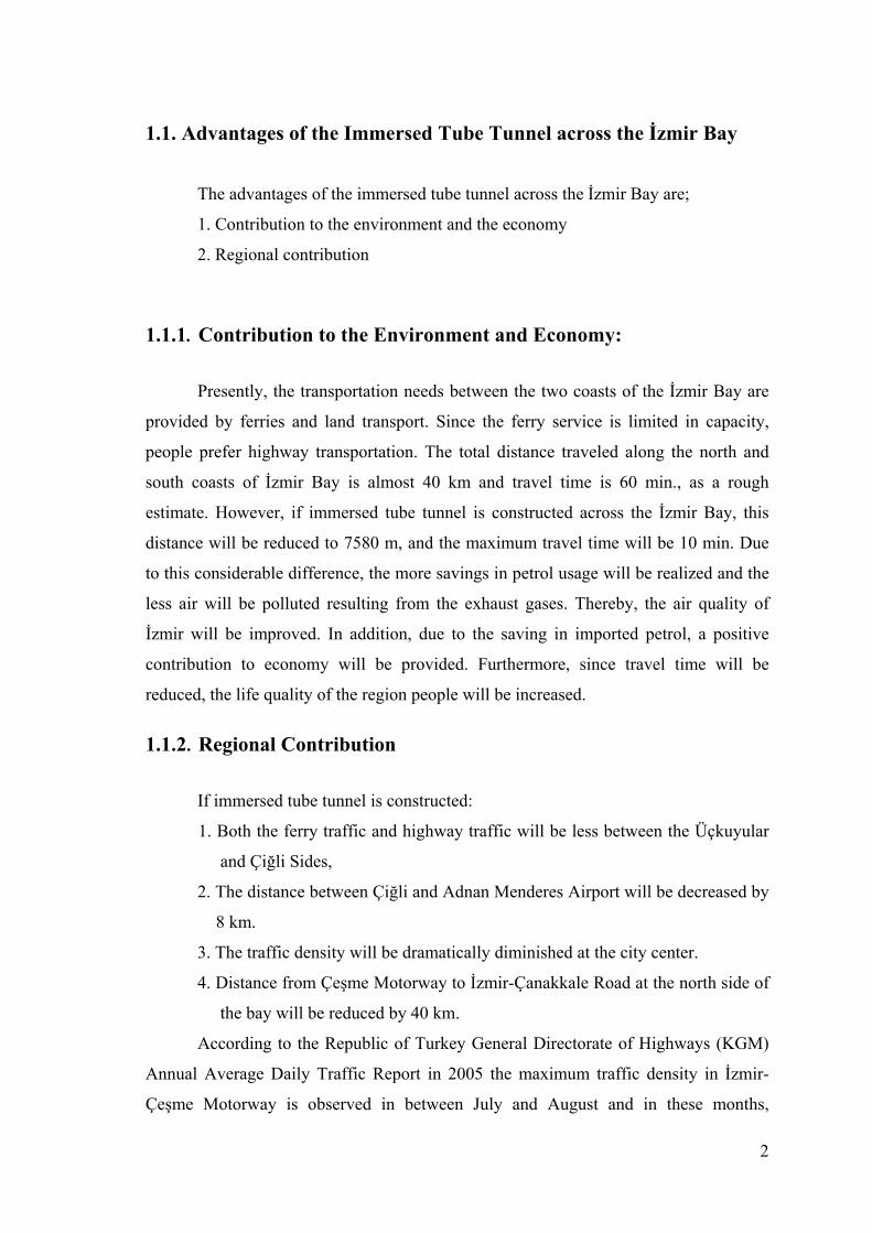
Presently, the transportation needs between the two coasts of the İzmir Bay are
provided by ferries and land transport. Since the ferry service is limited in capacity,
people prefer highway transportation. The total distance traveled along the north and
south coasts of İzmir Bay is almost 40 km and travel time is 60 min., as a rough
estimate. However, if immersed tube tunnel is constructed across the İzmir Bay, this
distance will be reduced to 7580 m, and the maximum travel time will be 10 min. Due
to this considerable difference, the more savings in petrol usage will be realized and the
less air will be polluted resulting from the exhaust gases. Thereby, the air quality of
İzmir will be improved. In addition, due to the saving in imported petrol, a positive
contribution to economy will be provided. Furthermore, since travel time will be
reduced, the life quality of the region people will be increased.
1.1.2. Regional Contribution
If immersed tube tunnel is constructed:
1. Both the ferry traffic and highway traffic will be less between the Üçkuyular
and Çiğli Sides,
2. The distance between Çiğli and Adnan Menderes Airport will be decreased by
8 km.
3. The traffic density will be dramatically diminished at the city center.
4. Distance from Çeşme Motorway to İzmir-Çanakkale Road at the north side of
the bay will be reduced by 40 km.
According to the Republic of Turkey General Directorate of Highways (KGM)
Annual Average Daily Traffic Report in 2005 the maximum traffic density in İzmir-
Çeşme Motorway is observed in between July and August and in these months,

3
approximately 40000 vehicles use this motorway daily. Similarly, the same report state
that the max traffic density realizes in between July and August in İzmir-Aydın
Motorway and the average number of vehicle per day using this motorway is 37000. On
the other hand, the capacity of İzmir Orbital Road is 40000 vehicles. Based on the these
investigations, it can be assumed that if immersed tube tunnel is constructed on between
Üçkuyular and Çiğli side, most probably at least 30000 vehicle will use this tunnel per
day.
To make a rough estimate about the cost of the immersed tube tunnel, it is
compared with the Marmaray Project. The unit cost of the immersed tube tunnel part of
the Marmaray Project is about 100 million USD per km. Since the total length of the
immersed tube tunnel recommended for the İzmir Bay is 7.6 km and its width about
1.33 times larger than the Marmaray, the approximate cost might be about
=⋅⋅ )6.7100)3.15/8.39(( 2 billion USD. However, if it is considered that the taken
Marmaray unit cost price of 100M USD/km doesn't cover the below explained cost
items of the IBITT tunnel, following costs can be added as an extra to the IBITT tunnel
cost:
1. Add cost of 7 M m3 of soft material dredging is estimated as Lump Sum: 0.2B
USD
2. Add cost of filling fine gravel to the sides of the tunnel, with a 1.5B m3
volume is estimated: 0.1B USD
3. Add cost of forming the first protective layer of the tunnel
(40mx1mx7600m=0.3M.m3 of sand-cement mixture) underwater: 0.05B. USD
4. Add cost of forming the second protective layer of the tunnel
(40mx1mx7600m=0.3M.m3 of armor rock) underwater: 0.05B USD
5. Add cost of expropriation of land as ROW (L=1km long and w=0.25 km wide
on both sides, with a total area=0.5km2): 0.01B. USD
6. Add cost of two ventilation buildings on either side or three ventilation shafts
in the sea (hsea=175 m.): 0.19B USD
7. Add cost of ground improvement (compaction grouting) up to 30 m depth
below seabed (w:50mxh:30mxL:7600m=11.4 M m3 ): 0.4B USD
If IBITT is not lowered by 10m from the existing seabed level (See Chapter 7),
the total cost is estimated as 3 billion USD. However, if it is lowered by 10 m from the
existing seabed level; this cost is increased to 3.3 billion USD.

4
The broad feasibility of the IBITT:
The total length of the tunnel: 7.58 km
The distance between Çiğli and İnciraltı by using surrounding highway: 50 km
The oil saving due to this difference:
USDMUSDkmlt 7.69)365()5.2()100/6()30000()58.700.50( =⋅⋅⋅⋅− (1.1)
The gain from the toll rate:
USDMdayvehicleUSDvehicle 55)365()/5()30000( =⋅⋅ (1.2)
Annual total benefits:
yearUSDM /7.124)557.69( =+ (1.3)
If 4.7 M USD /year (% 3.33) of the early capital gains is assumed as the early
maintenance cost of the tunnel, then the yearly capital gains become 120 M USD/year.
Thus, after construction the tunnel finances itself in the next:
yearsyearUSDM
USDBoryearsyearUSDM
USDB 5.27/120
3.325/120
3== (1.4)
Since the project pays itself back in roughly 25/27.5 years, it becomes attractive
(feasible) for Built-Operate-Transfer (BOT) type financing and 30 year BOT period is
quite reasonable.
It should be noted in here that since there was not enough data to make a
detailed cost analysis the cost estimation presented here is based on the Marmaray
Project. However, both the soil properties of the İzmir Bay and the structural properties
of the recommended tunnel are considerably different from the Marmaray Project.
Hence, a better cost estimation of the immersed tube tunnel can be provided after the
full feasibility report, which should include a detailed site investigation along the tunnel
route.

5
1.3. Scope of This Study
This study consists of five main parts:
1. Introduction
2. Properties of the proposed İzmir Bay Immersed Tube Tunnel
3. Current seabed properties
4. Static analysis for the preliminary design
5. Seismic analysis of the immersed tune tunnel
6. Ground improvement along the tunnel alignment
7. Conclusion
In the first part, immersed tube tunnels and their applicability to various types of
soils is described. Then, considering the soil type existing at the İzmir Bay, the
applicability of the immersed tube tunnel at that location was investigated using the soil
data obtained from the DLH.
In the second part, the possible route and geometric/technical properties of the
tunnel was determined.
In the third part, the ultimate and allowable bearing capacity of the soil was
calculated. Then, it was investigated that whether the current seabed soil has
liquefaction potential or not.
In the fourth part, in order to evaluate the displacement and stresses occurring
during and after construction, the static analysis was made by using Calculix finite
element program.
In the fifth part, the seismic requirement for the tunnel was investigated by an
equivalent static analysis method that is based on a seismic design procedure adopted in
Taiwan High Speed Railway Project, whereby the analyses were performed by using the
SAP 200 structural program.
In the sixth part, the aim of the ground improvement was explained and the most
appropriate improvement type for İzmir Bay is determined. Then, all analyses were
made again according to new situation of the seabed soil.
In the seventh part, which is the conclusion of the study, the obtained results of
the study have been summarized and some suggestions were made about the İzmir Bay.
6
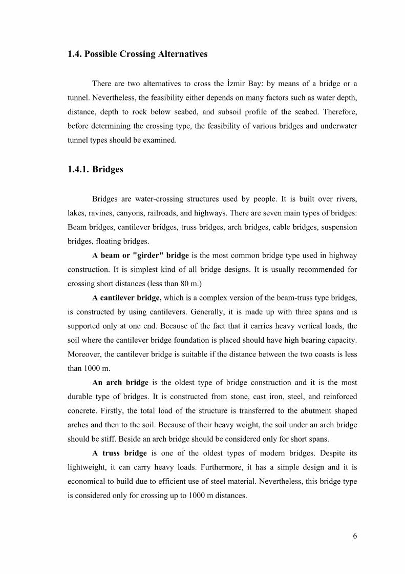
1.4. Possible Crossing Alternatives
There are two alternatives to cross the İzmir Bay: by means of a bridge or a
tunnel. Nevertheless, the feasibility either depends on many factors such as water depth,
distance, depth to rock below seabed, and subsoil profile of the seabed. Therefore,
before determining the crossing type, the feasibility of various bridges and underwater
tunnel types should be examined.
1.4.1. Bridges
Bridges are water-crossing structures used by people. It is built over rivers,
lakes, ravines, canyons, railroads, and highways. There are seven main types of bridges:
Beam bridges, cantilever bridges, truss bridges, arch bridges, cable bridges, suspension
bridges, floating bridges.
A beam or "girder" bridge is the most common bridge type used in highway
construction. It is simplest kind of all bridge designs. It is usually recommended for
crossing short distances (less than 80 m.)
A cantilever bridge, which is a complex version of the beam-truss type bridges,
is constructed by using cantilevers. Generally, it is made up with three spans and is
supported only at one end. Because of the fact that it carries heavy vertical loads, the
soil where the cantilever bridge foundation is placed should have high bearing capacity.
Moreover, the cantilever bridge is suitable if the distance between the two coasts is less
than 1000 m.
An arch bridge is the oldest type of bridge construction and it is the most
durable type of bridges. It is constructed from stone, cast iron, steel, and reinforced
concrete. Firstly, the total load of the structure is transferred to the abutment shaped
arches and then to the soil. Because of their heavy weight, the soil under an arch bridge
should be stiff. Beside an arch bridge should be considered only for short spans.
A truss bridge is one of the oldest types of modern bridges. Despite its
lightweight, it can carry heavy loads. Furthermore, it has a simple design and it is
economical to build due to efficient use of steel material. Nevertheless, this bridge type
is considered only for crossing up to 1000 m distances.

7
A suspension bridge is a type of bridge, which consists of two main cables
supporting the weight of the bridge and transfer the total load to anchorages and two
towers. It is recommended for large distances more than 1000 m. Due to the relatively
low deck stiffness, it is difficult to carry heavy live loads such as traffic loads. Thus, it
is not recommended for weak foundation soil such as loose silt and sand (Murowchick
2008).
A cable-stayed bridge is a variation of the suspension bridge and is designed
for intermediate lengths between 1000 m. and 2000 m. However, its principle and
construction method is quite different from a suspension bridge. For instance, the cable-
stayed bridges have tall towers like suspension bridges, but the roadway is attached to
the towers by a series of diagonal cables. Such bridges are much lighter and stiffer
compared to suspension bridges. This leads to a less deformation of the deck under the
live loads. In addition, they are economic and construction time is shorter than the
suspension bridges because cable stayed bridges do not need anchorages (Huang, et al.
2005).
A floating bridges is connected on top of pontoons that float on water. Due to
the advantage of natural buoyancy of water, the total load anchoraged to the soil can be
reduced. Therefore, it is more practical solution than other bridges types when the
waterbed is extremely soft. However, floating bridges is appropriate for large water
depths (30 m-60 m) (Watanabe and Utsunomiya 2003).
1.4.2. Underwater Tunnels:
Underwater tunnels are preferred when the soil profile of the waterbed or the
weather condition is not proper for a bridge to be constructed above water. There are
three alternative underwater tunnel types for crossing the water: Bored tunnels, floating
tube tunnels, immersed tube tunnels.
Bored tunnel shall be constructed when the ground or waterbed is appropriate
for excavating and preferred for deep tunnels. There are two alternative methods to
build a bored tunnel: Drilling-blasting method or by using a tunnel-boring machine.
Although a TBM machine with a circular cross-section excavates the soil without
disturbing it and produces a smooth tunnel wall, bored tunnel is only suitable for self-
retaining soils (TCRP Report/NCHRP Report 2006).

8
A submerged floating tunnel also known as an archimed bridge is a very new
concept in the world. Only, Norwegian and Chinese have submerged floating tunnel
projects in the design phase. Unlike the traditional underwater tunnels, submerged
floating tunnel (SFT) is not buried to the seabed; it is suspended above the water floor
and anchoraged to the ground with pontoons. It requires less substructure and
excavation compared to the other two alternatives. Nonetheless, SFT is only appropriate
for fjords, deep seas, and deep lakes (Hakkaart, et al.1993).
An immersed tube tunnel is made up of many prefabricated tubes constructed
on land, which are then floated and moved to its dredged location by romorks in the sea.
The tubes are lowered and connected with each other underwater. Then, the water is
pumped out and the segments are covered with the backfill materials. It is preferred if
the water depth is not larger than 60 m. and the waterbed is suitable for dredging, such
as soft sandy, silty or alluvial soils(Baltzer and Hehengeber 2003).
1.5. Soil Profile of the İzmir Bay Bottom
İzmir Bay seabed consists of mixture of very loose silt, sand and alluvial
materials, which are either non-cohesive or have very low cohesion values. Moreover,
the rock layer depth is found approximately at 50 m below the sea level in the
Üçkuyular side and 250 m-280 m below the sea level in the Çiğli side. Therefore, its
ultimate bearing capacity is very low. Moreover, since the water depth of the İzmir Bay
is less than 25 m, this is an advantage for an immersed tube tunnel to be built.
Considering these properties, it has been decided that the immersed tube tunnel type of
construction is the most suitable one for crossing the İzmir Bay.
1.6. Application History of the Immersed Tube Tunnel
The important immersed tube tunnels were listed below (Grantz, et al. 1993):
The immersed tube tunnel was heard firstly in the world in 1910 with the
construction of the Detroit River Tunnel between USA and Canada. This immersed tube
tunnel has been constructed 24 m below the water level and consists of eleven pieces of
tubes. Each tube length is 80 m, height is 9.4 m, and width is 17 m, yielding to a total
length of 800 m.

9
On the other hand, the first immersed tube tunnel in Europe is the Mass Transit
Tunnel in Netherland constructed in 1941. The total length of this highway tunnel is 584
m. The tunnel consists of nine concrete box tubes, which are 61.35 long, 8.39 m in
height and have a width of 24.77 m.
In 1958, prestressed concrete boxes were used for the first time in the
construction of an immersed tube tunnel in Cuba. The total length of the tunnel is 520
m. The lengths of the tubes varies between 90 m and 107.5 m, the width is 21.85, and
the height is 7.10 m. This highway tunnel was built 23 m under the sea level.
The Dees Tunnel in Canada was the first project considering the earthquake
loads and was constructed 22 m below the sea level, with a total length of 629 m. It
includes concrete tubes, with lengths of 104.9 m, height of 7.16 m and width of 23.80
m.
The Scheldt E3 (JFK) Tunnel, built in 1969 in Belgium, has the biggest tubes,
which had ever been constructed in the world among all of the immersed tube tunnels.
The width of the prestressed concrete boxes was 47.85 m, height was 10.1 m, while the
length varies between 99 m and 115 m and the weight of each tube was nearly 47000
tons.
The Bay Area Rapid Transit (BART) Tunnel is the longest existing immersed
tube tunnel in the world. The tunnel is in use in San Francisco California and
constructed in 1970. The total tunnel length is 5825 m. and it has been operating as a
railway. The tunnel consists of 58 tubes and each has a length of 110 m, a height of 6.5
m and width of 14.6 m. At a maximum depth of 41 m below the sea level, the Bay Area
Rapid Transit Tunnel is one of the deepest vehicular tubes in service today.
The Oresund Tunnel constructed between Denmark and Sweden is the world’s
largest immersed tunnel in terms of volume. The total length of immersed tube tunnel
section is 3510 m and the widht of the tubes are 40 m.
The first example of the immersed tube tunnels constructed in Turkey is the
Marmaray Project that is being built on the İstanbul Bosporus Waterway. It will be the
deepest immersed tube tunnel in the world when the construction is completed
(Marmaray 2007).
There were 108 immersed tube tunnels in the world until 1997. 48 of them in
Europe, 27 of them in North America, 20 of them in Japan, 9 of them in South
Asia(except Japan) and 4 of them in other countries (Marmaray 2007).
10
CHAPTER 2
PROPERTIES OF THE PROPOSED İZMİR BAY
IMMERSED TUBE TUNNEL
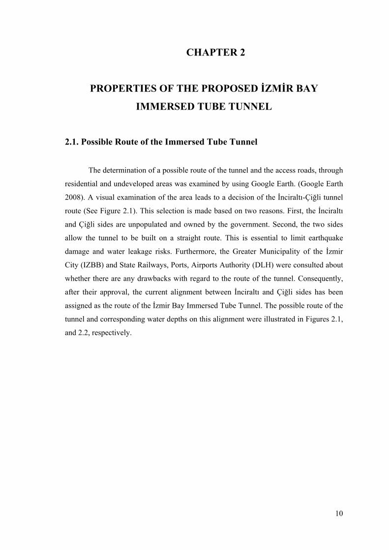
2.1. Possible Route of the Immersed Tube Tunnel
The determination of a possible route of the tunnel and the access roads, through
residential and undeveloped areas was examined by using Google Earth. (Google Earth
2008). A visual examination of the area leads to a decision of the İnciraltı-Çiğli tunnel
route (See Figure 2.1). This selection is made based on two reasons. First, the İnciraltı
and Çiğli sides are unpopulated and owned by the government. Second, the two sides
allow the tunnel to be built on a straight route. This is essential to limit earthquake
damage and water leakage risks. Furthermore, the Greater Municipality of the İzmir
City (IZBB) and State Railways, Ports, Airports Authority (DLH) were consulted about
whether there are any drawbacks with regard to the route of the tunnel. Consequently,
after their approval, the current alignment between İnciraltı and Çiğli sides has been
assigned as the route of the İzmir Bay Immersed Tube Tunnel. The possible route of the
tunnel and corresponding water depths on this alignment were illustrated in Figures 2.1,
and 2.2, respectively.

11
Max. 6 m.
Max. 9 m.
Figure 2.1. The possible route of tunnel
(Source: Google Earth 2008)
Figure 2.2. The water depths on the possible route of tunnel
Max 17 m

12
2.2. Geometric Properties of the Tube
The İzmir Bay Immersed Tube Tunnel (IBITT) is composed of two land tunnel
parts on each shore and an immersed-tube tunnel part at the center. The total length is
7580m, including an immersed tunnel section of 5560m in the middle. The tunnel has
about 76 tunnel units. Each unit includes a two lane railway in the middle
(width=10.6m) and three lane highways (width=13m) one on each side. The shape of
each tunnel element has 39.8 m width, 10m height and the length varies 100m~120m,
and its weight is approximately 38195t. The technical properties and typical cross
section of the immersed tube tunnel unit were illustrated in Figure 2.3 and 2.4,
respectively.
From the İnciraltı shore to the Çiğli shore, the tunnel starts with a 2.5%
declination (station: km 0+000 m) for 1120 m. This is station: km 1+120 m, at which
the inclination becomes zero for 2240 m (station: km 3+360 m). Afterwards, the road
climbs with a 1% slope towards the Çiğli exit (station: km 7+580m). The deepest point
of the top of the tunnel is 18.5 m. below the sea level and this depth is constant between
station: km 1+120 m and station: km 3+660m. The longitudinal section of the immersed
tube tunnel was illustrated in Figure 2.5
It should be noted in here that during the full feasibility report, detailed site
investigation should be done. This study should include studies like bathymetric
(seawater depth) and seismic fault line studies, current seawater quality of the dredged
sediment disposal areas, shipping lane surveys etc. A contractor or its appointed
subcontractor with a sub consultant can do these surveys, but overall independent
consultant authorized by the client (DLH) should check all studies, reports,
recommendations, and the works during the construction stage. It is emphasized that the
current max. seawater depth record 18.5 m is not sufficent for any big cargo/contanier
ship or for very large crude oil carrier if the existing İzmir Port does not move to out of
the bay and will continue to be used in the future. In this case, there is a need of min 25
m seawater depth at the ship lane passage, indicating that IBITT should be further
lowered by 10 m, making the max seawater depth equal to 28.5 m.

13
Figu
re 2
.3. T
he t
echn
ical
pro
perti
es o
f the
IBIT
T
14
Figu
re 2
.4. T
he c
ross
-sec
tion
sect
ion
of t
he IB
ITT
0,000
RO
CK
LA
YER
CR
OSS
-SEC
TIO
N A
-A
-50,000
-3,6
00
-1,6
00
BA
CK
FILL
M
ATE
RIA
LB
AC
KFI
LL
LAY
ER
New
wat
er d
epth
Nat
ural
wat
er d
epth
SAN
D L
AY
ER
VER
Y L
OO
SE S
ILTY
-SA
ND
LA
YER
SAND FOUNDATION
AR
MO
R S
TON
E LA
YER
AR
MO
R S
TON
E LA
YER

15
Figu
re 2
.5. T
he lo
ngitu
dina
l sec
tion
of t
he IB
ITT
100
100
120
% 0
IMM
ERSE
D
TUN
NEL
UN
ITS
AA
C
4+780
0+120
0+220
0+320
0+420
0+520
0+620
0+720
0+820
0+920
1+020
1+120
1+240
1+340
1+440
1+540
1+640
1+740
1+840
1+940
2+040
2+140
2+240
2+340
2+440
2+540
2+640
2+740
2+840
2+940
3+060
3+160
3+260
3+360
3+460
3+560
3+660
3+760
3+860
4+060
4+160
4+260
4+360
4+460
4+560
4+660
4+880
4+980
3+960
0
-1
-2
-4
-3
-5
-6
-7
-8
-9
-10
-11
-12
-13
-14
-15
-16
-17
-18
-19
-20
-21
-23
-24
-25
-26
-27
-28
-29
-30
-31
-32
-33
-34
-35
-36
-37
123456789101112
%2.
5
IMM
ERSE
D T
UB
E TU
NN
EL
%1
AR
MO
R S
TONE
SOIL
LIN
E
CHAINAGE0+000
SOIL
LIN
E
IMM
ERSE
D
TUN
NEL
UN
ITS
AR
MO
R S
TONE
AR
MO
R S
TON
E
5+080
5+180
5+280
5+380
5+480
5+580
5+680
5+780
5+880
5+980
6+080
6+180
6+280
6+380
6+480
6+580
6+680
6+780
6+880
6+980
7+080
7+180
7+280
7+380
7+480
7+580
SO
IL
C

16
CHAPTER 3
CURRENT SEABED-SOIL PROPERTIES
3.1. Allowable Bearing Capacity
Using soil-boring data from the existing 3 boreholes nearest to the tunnel
alignment, it was seen that the subsoil is mostly non-cohesive very loose to loose silty-
sand or sandy-silt, with depths to bedrock varying between about 50 m on the
Ückuyular side and about 280 m on the Çigli side. However, these preliminary site
results should be confirmed by additional site investigations along the route, during the
feasibility study or the preliminary design stages. Now, before describing bearing
capacity values, firstly some definitions should be given;
• Bearing capacity is the capacity of soil to withstand the pressure from any
engineered structure placed upon it, without producing any shear failure and
large settlement.
• The ultimate bearing capacity (qu) is the maximum pressure value that can be
applied to the soil without causing shear failure.
• The allowable bearing capacity (qa) is the maximum permissible pressure that
can be applied to the soil so that shear failure does not occur and the maximum
tolerable settlement is not exceeded.
The allowable bearing capacity of a soil can be calculated in terms of two
different criteria:
a) The allowable bearing pressure based on ultimate capacity: This method
is based on the relationship between the shear strength and allowable bearing capacity
of the soil. According to this criterion, the allowable bearing capacity of the soil is equal
to the ultimate bearing capacity of soil divided by a factor of safety.
b) The allowable bearing pressure based on tolerable settlement: In this
method, it is assumed that the allowable bearing capacity of soil is equal to the
maximum pressure without leading to intolerable settlement. (less than 2.5 cm)

17
It is recommended that, the allowable bearing capacity of soil should be
calculated according to two different methods, respectively. In order to stay on the safe
side, the smaller one should be used.
a. The allowable bearing pressure based on ultimate capacity: According to
TENG (1962), the ultimate bearing capacity divided by a selected factor of safety, gives
the allowable bearing capacity.” A factor of safety of 3 is used under normal loading
conditions and a factor of safety of 2 under combined maximum load” (TENG 1962).
For long footings:
)()100(5'3 22 psfRDNRBNq wwult ⋅⋅+⋅+⋅⋅⋅= (3.1)
)/())100(08.0'048.0 222 mtRDNRBNq wwult ⋅⋅+⋅+⋅⋅⋅= (3.2)
FSq
q ulta = (3.3)
where N is the standard penetration resistance, (number of blows per foot), B
is the width of footing in meters unit, D is the depth of footing measured from ground
surface to bottom of footing in meters, and wR and wR' are the correction factors for
position of water level that can be obtained from Fig 3.1, and FS is the factor of safety.
b. The allowable bearing pressure based on tolerable settlement: Allowable
bearing capacity for maximum settlement of 2.5 cm is given by TENG (1962) as;
)(2
1)3(7202
psfRB
BNq wcora ⋅⎟⎠⎞
⎜⎝⎛ +⋅−⋅= (3.3)
)/()2
3048.0)3(5.3 22
mtRB
BNq wcora ⋅⎟⎠⎞
⎜⎝⎛ +⋅−⋅= (3.4)
where corN is the corrected SPT_N value,

18
⎟⎟⎠
⎞⎜⎜⎝
⎛+
⋅=7
35p
NNcor (3.4.a)
where, N is the SPT value obtained from the field, p′ is the effective overburden
pressure in 2/mt unit and can be calculated by the following formula.
hp ⋅=′ 'γ (3.4.b)
where, h is the half of the height between the sea level and the rock layer in meter, and
'γ is the effective density of the soil in 3/ mt and it can be calculated from the following
formula,
wsat γγγ −=' (3.4.c)
where, satγ is the density of the saturated soil and wγ is the density of the sea water.

19
Figure 3.1. Correction factor for position of water level: (a) depth of water level
with respect to dimension of footing; (b)water level above base of
footing (c): water level below base of footing . (Source: Teng 1962)
3.1.1. SPT Results of the İzmir Bay
SPT-N value: A standard sampler is driven 450 mm into the ground at the
bottom of drilled borehole by a drop hammer with a weight of 63.5 kg falling through a
height of 76 cm. The number of blows is recorded at each 150 mm increments. The SPT-
N is the number of blows required to achieve penetration from 15-45cm (Sivrikaya and
Toğrol 2003).
h
B
Water level ( i )
Water level ( ii )
da
db
D
B
( a )
0,5
0,6
0,7
0,8
0,9
1,0
0 0,2 0,4 0,6 0,8 1,00,5
0,6
0,7
0,8
0,9
1,0
0 0,2 0,4 0,6 0,8 1,0
da / D db / B
( b ) ( c )
Red
uctio
n fa
ctor
Rw
Red
uctio
n fa
ctor
Rw
For case ( i ) only For cases ( ii ) ( iii )
Water level ( iii )

20
For this study, there was no opportunity to make standard penetration tests
(SPT) along the tunnel route. Therefore, test results that were obtained in the past is
investigated by. Among these, data nearest to the tunnel route were used and the SPT
results are presented in Table 3.1. These values are used to calculate the allowable
bearing capacity of the seabed soil of the proposed IBITT across the İzmir Bay can be
calculated. The borehole locations of the SPT are shown in Figure 3.2.
Figure 3.2. The locations of the 3 existing SPT boreholes nearest the IBITT route
SK8
SK17
SK18

21
Table 3.1 The SPT results obtained from DLH İzmir
(Source: DLH 1985)
i) At the borehole location SK-18, the penetration values are:
SPT-1 (at 4.10 m.) 211)4530()3015( =+=−+−= NNN
SPT-2 (at 5.50 m.) 271512)4530()3015( =+=−+−= NNN
SPT-3 (at 7.10 m.) 341717)4530()3015( =+=−+−= NNN
SPT-4 (at 8.60 m.) 361917)4530()3015( =+=−+−= NNN
SPT-5 (at 10.10 m.) 321715)4530()3015( =+=−+−= NNN
Borehole Location : SK-18 Depth(m) Sample Number The Number of Blow
0-15 15-30 30-45 4.10 SPT-1 1 1 1 5.50 SPT-2 10 12 15 7.10 SPT-3 15 17 17 8.60 SPT-4 12 17 19
10.10 SPT-5 15 15 17 11.60 SPT-6 15 16 16 13.10 SPT-7 23 11 12 14.60 SPT-8 18 17 17 16.10 SPT-9 15 15 18 17.60 SPT-10 15 15 18
Borehole Location : SK-8 Depth(m) The Number of sample The Number of Blow
0-15 15-30 30-45 3.00 SPT-1 1 1 1 4.50 SPT-2 1 1 2 6.00 SPT-3 2 2 2 7.50 SPT-4 2 2 3 9.00 SPT-5 2 3 4
10.50 SPT-6 2 2 3 12.00 SPT-7 3 3 4
Borehole Location : SK-17 Depth(m) The Number of sample The Number of Blow
0-15 15-30 30-45 9.85 SPT-1 - - -
11.35 SPT-2 - - - 12.85 SPT-3 1 1 1 14,35 SPT-4 1 1 1 15.85 SPT-5 1 1 1 15.85 SPT-6 1 1 1
22
SPT-6 (at 11.60 m.) 321616)4530()3015( =+=−+−= NNN
SPT-7 (at 13.10 m.) 221111)4530()3015( =+=−+−= NNN
SPT-8 (at 14.60 m.) 341717)4530()3015( =+=−+−= NNN
SPT-9 (at 14.60 m.) 331815)4530()3015( =+=−+−= NNN
SPT-10 (at 17.60 m.) 331815)4530()3015( =+=−+−= NNN
ii) At the borehole location SK-8, the penetration values are:
SPT-1 (at 3.00 m.) 211)4530()3015( =+=−+−= NNN
SPT-2 (at 4.50 m.) 321)4530()3015( =+=−+−= NNN
SPT-3 (at 6.00 m.) 422)4530()3015( =+=−+−= NNN
SPT-4 (at 7.50 m.) 532)4530()3015( =+=−+−= NNN
SPT-5 (at 9.00 m.) 743)4530()3015( =+=−+−= NNN
SPT-6 (at 10.50 m.) 532)4530()3015( =+=−+−= NNN
SPT-7 (at 12.00 m.) 743)4530()3015( =+=−+−= NNN
iii) At the borehole location SK-17, the penetration values are:
SPT-1 (at 9.85 m.) 000)4530()3015( =+=−+−= NNN
SPT-2 (at 11.35 m.) 000)4530()3015( =+=−+−= NNN
SPT-3 (at 12.85 m.) 211)4530()3015( =+=−+−= NNN
SPT-4 (at 14.35 m.) 211)4530()3015( =+=−+−= NNN
SPT-5 (at 15.85 m.) 211)4530()3015( =+=−+−= NNN
SPT-6 (at 17.85 m.) 211)4530()3015( =+=−+−= NNN
Based upon the three testing stations (SK18, SK8, SK17), average values of the
N values can be taken so that,
i) SPT_N=29 for areas that are close to the İnciraltı side,
ii) SPT_N=4 for areas that are close to the Çiğli side
iii) SPT_N=2 for the middle of the IBITT route.
3.1.2. Allowable Bearing Capacity of the Seabed Soil of the İzmir Bay
The allowable bearing capacity will be calculated for SPT_N= 4 only. The other
locations are compared according to this result.

23
a.) First method: The allowable bearing Pressure based on ultimate capacity
The ultimate bearing capacity based on shear failure of the soil is calculated by
Eq 3.2:
)/()100(08.0'048.0 222 mtRDNRBNq wwult ⋅⋅+⋅+⋅⋅⋅=
mB 8.39= mD 5.28=
1=Dda 5.0=wR 0' =wR from Figure (3.1)
)/(5.05.28)4100(08.008.394048.0 222 mtqult ⋅⋅+⋅+⋅⋅⋅=
2/132 mtqult =
The allowable bearing capacity of the soil is calculated by Eq 3.2:
FSq
q ulta =
where FS is taken as 3. (Bowles 1988)
2/443
132 mtqa ==
b) Second Method: The allowable bearing capacity based on 2.5 cm tolerable
settlement
First, p′ is calculated by Eq 3.4.b:
hp ⋅=′ 'γ
3/773.0027.1800.1' mt=−=γ

24
Assuming the rock layer is present at a depth of 150 m below the sea level, h is
calculated as follows.
mh 752
150==
2/5875773.0 mtp =⋅=′
If the overburden pressure exceeds 28.12 t/m2 (40 psi), it takes the value of
28.12 t/m2 (40 psi) (Teng 1962). Thus; p ′ is taken as 28.12 t/m2 (40 psi)
Second, corrected SPT_ N value ( corN ) is found by Eq 3.4.a:
⎟⎠⎞
⎜⎝⎛
+⋅=⎟⎟
⎠
⎞⎜⎜⎝
⎛+
⋅=1040
50410
50p
NNcor
4=corN
Last, the allowable bearing capacity of the soil is calculated by Eq 3.4:
)/()2
3048.0)3(5.3 22
mtRB
BNq wcora ⋅⎟⎠⎞
⎜⎝⎛ +⋅−⋅=
mB 8.39= 5.0=wR
5.08.3923048.08.39)34(5.3
2
⋅⎟⎠⎞
⎜⎝⎛
⋅+
⋅−⋅=aq
2/44.0 mtqa =
A comparison of the above based on two different approaches shows that the
second approach yields a smaller value. This means that the soil fails because of

25
intolerable settlement, before it fails due to shear failure. Thus, the result found from the
second approach is used as the allowable bearing capacity of the soil.
The allowable bearing capacity of soil is very small, and it seems clear that it is
smaller than the net total pressure applied at foundation level, hence ground
improvement is definitely recommended
The SPT-N value is assumed as 2 in the Çiğli coastal area side. Therefore, in this side,
the allowable bearing capacity of the soil is less than 0.44 t/m2. It can be said that if the
SPT-N is less than 3 the soil does not have enough capacity to carry the net foundation
pressure applied on the seabed soil. Based on the existing SPT-N value results, it can be
concluded that the allowable bearing capacity of the Çiğli seabed soil is less than the
net pressure applied to it. Thus ground improvement is needed. In the İnciraltı side the
SPT-N value was assumed as to be 29, Hence, the soil has enough bearing capacity to
carry the pressure transferred to it. However, since the soil consists of sand and gravel
in this part, it is recommended to compact the soil by making grouting up to at least 30
m (0.75B) depth below the seabed. There are no SPT results for the middle alignment of
the tunnel (based on the DLH study); and therefore the allowable bearing capacity of the
soil could not be calculated
3.2. Liquefaction Potential of the Seabed Soil
If loose saturated and unconsolidated granular soil is subjected to cyclic loading
such as earthquake loading, its pore pressure will increase. As a result of this, the soil
particles lose its effective stress and the medium acts as a liquid. (Das 1983). This
behavior is called liquefaction and generally occurs in loose to moderately compacted
granular soils (such as silty sands or sands and gravels) under water, with poor drainage
conditions. Figure 3.3 explains the liquefaction process of the soil.
To decide whether the soil has been under the liquefaction risk or not, there are
several methods, such as laboratory investigations and observations on the field. Based
on the existing test results, the liquefaction risk of the İzmir Bay’s seabed is examined
by using two different analyses:
1. Liquefaction analysis by using depth and SPT data relationship
2. Liquefaction analysis by using the simplified procedure
26
Water-saturated sediment Liquefaction
Figure 3.3. Liquefaction process of the soil
(Source: Tulane University 2004)
3.2.1. Liquefaction Analysis by using Depth and SPT Data
Relationship
In this method, the liquefaction potential of the soil is examined by using a
relationship between the SPT-N values and their corresponding depth (Tezcan and
Özdemir 2004). For instance, by using three SPT data, which were provided from three
different locations (nearest to the route) of the İzmir Bay, the liquefaction risk of the
tunnel soil can be revealed by means of the graph in Figure 3.4. SK18 is the name of the
borehole location near the İnciraltı side, SK17 is the name of the borehole location
between the İnciraltı side and the Çiğli side, and SK8 is the name of the borehole
location near the Çiğli side. The locations of the boreholes are shown in Figure 3.2.
Two curves plotted in Figure 3.4 show the degree of liquefaction potential of the
soil. The processed data from Table 3.1 is inserted into this graph, revealing the degree
of liquefaction risk of the soil. It can be seen that the Çiğli side is under high risk and
the İnciraltı side is under low risk. According to this depth and SPT data relationship,
ground improvement appears to be necessary
Water fills in the pore space between soil
particles. Friction between particles holds
water-saturated sediment together.
Water completely surrounds all soil
particles and eliminates all particles to
contact. Sediment flows like a fluid.

27
Figure 3.4. Relationship between the possibility of liquefaction and N values
(Source: Tezcan and Özdemir 2004)
3.2.2. Liquefaction Analysis by using Simplified Procedure
The simplified procedure is originally developed by Seed and Idriss in 1971
following the disastrous earthquake in Alaska, USA and in Nigata, Japan in 1964. This
procedure is based on the relationship between the cyclic resistance ratio (CRR) and
cyclic stress ratio (CSR). Dividing the CRR to CSR, the factor of safety FS is found.
At locations, where FS is less than unity, liquefaction is expected to occur (Tezcan
and Özdemir 2004).
The factor of safety, FS , expressed as the capacity over demand is:
CSRCRR
DemandCapacity
FS == (3.5)
FS should be bigger than 1 to avoid liquefaction risk.
DEP
TH (m
)
STANDARD PENETRATION VALUE (N)
SK-8:Çiğli side
SK-17:Çiğli-Üçkuyularside
SK-18:Üçkuyular side
MEDIUM LIQUEFACTION RISK
LOW LIQUEFACTION RISK
HIGH LIQUEFACTION RISK
50
18.0
15.0
12.0
30 402010
9.0
6.0
3.0
00

28
3.2.2.1. Earthquake Induced Shear Stress Ratio (CSR)
A transient earthquake motion is converted to an equivalent series of uniform
cycles of shear stress. The number of equivalent cycles, a function of the duration of
motion is correlated with the magnitude of the earthquake (Lee and Seed, 1967). The
actual time history of shear stress at any point in a soil deposit during an earthquake will
have an irregular form. Therefore, the average equivalent stress, br =65% of the
maximum shear stress, is used for wM =7.5 earthquake magnitude expected in İzmir
Bay. To calculate the cyclic stress ratio (CSR) the following formula is developed in the
field, due to earthquake shaking (Tezcan and Özdemir 2004).
dov
ovb
vo
av rg
arCSR ⋅⋅==
'.
'max
σσ
στ
(3.6)
dvobav rg
ar ⋅⋅⎟⎟
⎠
⎞⎜⎜⎝
⎛⋅= στ max (3.7)
where, avτ : the average horizontal shear stress developed on the soil element,
vo'σ : effective overburden pressure,
ovσ : total vertical overburden pressure,
maxa : peak ground acceleration
g : acceleration of gravity
dr : depth reduction coefficient (see Sec. 3.2.2.2.)
br : coefficient for effective average level of acceleration,
)1(1.0 −⋅= wb Mr (3.8.a)
5.765.0 == wb Mforr (3.8.b)

29
3.2.2.2. Depth Reduction Factor
The depth reduction factor, dr , is introduced to take into account the fact that the
amplitudes of horizontal accelerations decrease, as the depth below the ground surface
increases (Similar to the acceleration response values in high-rise buildings). Seed and
Idris (1971) recommended using the following dr values, which account for the
flexibility of the soil profile, in regard to routine practice and non-critical projects
(Tezcan and Özdemir 2004).
zrd ⋅−= 00765.01 for 15.9≤z (3.9.a)
zrd ⋅−= 0267.0174.1 for 9.15 23≤≤ z (3.9.b)
zrd ⋅−= 0082.0744.0 for 23 30≤≤ z (3.9.c)
50.0=dr for z 30≥ (3.9.d)
where z is the depth to the midpoint of the layer below the seabed surface in m.
3.2.2.3. Cyclic Resistance Ratio (CRR)
To determine the capacity of seabed soil to resist liquefaction, cyclic resistance
ratio-CRR is determined by use of field correlations from insitu tests or laboratory tests
on representative samples of the soil deposits. The three most routinely used methods to
evaluate the liquefaction resistance, CRR, are:
i: The standard penetration test (SPT),
ii: The cone penetration test (CPT),
iii: The seismic shear wave velocity (Vs) test (Tezcan and Özdemir 2004).
For this work, the CRR value is calculated by using the SPT results.
Corrected factors for SPT Values are;
( ) mSRBEN NCCCCCN ⋅⋅⋅⋅⋅=601 (3.10)
30
where,
( )601N : Corrected SPT number
NC : Overburden correction factor
EC : Correction factor for the SPT hammer energy ratio
BC : Correction factor for the borehole diameter
RC : Correction factor for the rod length
SC : Correction factor for the sampling method
mN : Insitu measured Standard Penetration resistance value
The correction factors sRBEN CCCCC ,,,, are summarized in Table 3.2.
After calculating the corrected SPT number, the CRR can be found by using
charts developed by different researches.
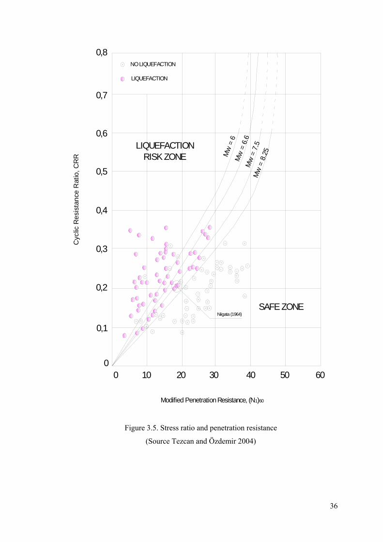
Curves by Seed et al. (1983): Practical charts are proposed by Seed et. al.
(1983) regarding evaluation of the liquefaction potential for different magnitude
earthquakes, by representing the behavior of sands with D50>0.25 mm, under level
ground conditions, and penetration resistance, N1, as shown in Figure 3.5 (Tezcan and
Özdemir 2004).

31
Table 3.2. The correction factor values for corrected SPT values
(Source: Tezcan and Özdemir 2004)
Symbol Correction factor value
CN (overburden pressure
correction factor)
vo'σ is in kg/cm2
'1
voNC
σ= (Liao and Whitman,1986)
⎟⎟⎠
⎞⎜⎜⎝
⎛⋅=
voNC
'20log77.0σ
(Peek ,et al. 1974)
voNC 'log25.11 σ⋅−= (Tokimatsu and Yoshimi,1983)
voNC
'7.07.1σ+
= (Seed and Idriss, 1983)
CE (Energy ratio
correction factor)
60.0ratioEfficiencyCE =
where efficiency ratio(ER) is the for percentage of the theoratical SPT
impact hammer energy actuallay transmitted to hammer Equipment ER CE
Donnut hammer(1) 0.30 to 0.60 0.5 to 1.0 Donnut hammer(2) 0.70 to 0.85 1.2 to 1.4 Safety hammer 0.40 to 0.75 0.7 to 1.2 Automatic-trip Donut hammer 0.50 to 0.80 0.8 to 1.3
CB (Borehole diam. correction factor)
D=65~115 mm CB=1.0 D=150 mm CB=1.05 D=200 mm CB= 1.15
CR (Rod lenght correction
factor)
L<3 m CR=0.75 3<L≤ 4 CR=0.80 4<L≤ 6 CR=0.85 6<L≤ 10 CR=0.95 10<L≤ 30 CR=1.00
CS (Sampling method correction factor)
Standard sampler CS=1.00 Sampler without lines CS=1.10 Loose soils CS=1.30 Dense soils

32
The application of the simplified procedure for this study based on the İzmir
Bay’s soil properties is described below;
i) The cyclic stress ratio (CSR) is;
The total stress under 2.5B depth of the tunnel base:
)()()()( 5321 soiltubebase
conceretetubeconcretesandstonearmorwatervo h
AV
hhh γγ
γγγσ ×+⎟⎟⎠
⎞⎜⎜⎝
⎛ ⋅+×+×+×= −−
(3.11)
)60.1100(1008.39
5.215278)1.25.0()6.25.0()027.15.17( ×+⎟⎠⎞
⎜⎝⎛
⋅⋅
+×+×+×=voσ
22 /19/92.189 cmkgmtvo ==σ
The effective stress under 2.5B depth of the tunnel base,
22 /8.5/95.57)027.1)1001015.17(( cmkgmtvovo ==×+++−=′ σσ (3.12)
The depth reduction factor:
5.128100105.05.05.1754321 =++++=++++= hhhhhz
mz 30≥ 50.0=rd (from Eq 3.9.d )
The cyclic stress ratio is calculated by Eq 3.6. as below;
dov
ovb
vo
av rg
arCSR ⋅⋅==
'.
'max
σσ
στ
ga 34.0max = (from Table 3.3.)
65.0=br (from Eq 3.8.b)

33
50.095.5792.18934.065.0 ⋅⎟
⎠⎞
⎜⎝⎛⋅⎟⎟
⎠
⎞⎜⎜⎝
⎛ ⋅⋅=
ggCSR
362.0=CSR
Table 3.3 Ground Acceleration Coefficients and Peak Ground Acceleration
(Source:Taiwan High speed Rail Project Contract C240 2003)
Level of Earthquake Ground Acceleration
Coefficient (Zt)
Peak Ground Acceleration (amax)
m/s2
Type I (severe) 0.34 3.34
Type II (moderate) 0.11 1.11
ii) The cyclic resistance ratio (CRR) is;
Firstly, the correction factors are obtained from Table 3.2.
The overburden correction factor NC is:
To calculate the overburden pressure correction factor value the formula
developed by Liao and Whitman was used. Thus,
415.08.5
1'
1===
voNC
σ (3.11)
The energy ratio correction factor EC is:
60.0RatioEfficiencyCE = (3.12)
Assume that the donut hammer was used for the SPT and ER=0.60.
for 0.160.0 =→= ECER (3.13)

34
The borehole diameter. correction factor BC is:
Note that, N is too small when an oversize borehole is drilled (Bowles 1988).
Hence,
15.1=BC (3.14)
The rod length correction factor RC is:
Note that, N is too high for L>10 m (Bowles 1988). Thus,
00.1=RC (3.15)
For loose soils sampling method correction factor sC is:
10.1=sC (3.16)
Assumption: At 17.5 m. depth (the part, where the inclination of the tunnel is
zero), the N value was taken as 4 (as an average value), based on the other SPT results
due the fact that there was no SPT results for this part of the tunnel.
Finally, the corrected SPT_N value ( )601N is found from Eq 3.10:
( ) mSRBEN NCCCCCN ⋅⋅⋅⋅⋅=601 410.10.115.10.1415.0)( 601 ⋅⋅⋅⋅⋅=N
( ) 1.2601 =N
From Figure 3.5. the CRR value is,
for ( ) 1.2601 =N and 02.05.7 =→= CRRM w
At last, factor of safety can be calculated from Eq 3.5 as below;
362.0=CSR

35
02.0=CRR ….
06.0362.002.0
===CSRCRRFS
25.106.0 <=FS
Thus, the soil has high liquefaction potential.
Three SPT testing borehole results along the IBITT route are evaluated for this
study. They are used to calculate the allowable bearing pressure and give an idea about
the side’s liquefaction potential. However, there are a number of drawbacks in using
these data. First, the numbers of boreholes are not enough. Second, the boreholes do not
reach to the depth of the IBITT, which is designed to be at a depth of 28.5 meters.
The calculated allowable bearing capacities may not be reliable. These
capacities are based on equations that are developed for line footings. In the current
study, on the other hand, the magnitude of the tunnel width is 10-30 times larger than a
regular footing. As is the case with the allowable bearing capacity analysis, the stress
ratio and penetration resistance analysis, also suggests that the site of interest has high
liquefaction potential. Based on the results of the two methods, ground improvement
appears to be necessary along the IBITT route.
36
LIQUEFACTIONRISK ZONE
SAFE ZONE
0
0,1
0,2
0,3
0,4
0,5
0,6
0,7
0,8
0 10 20 30 40 50 60
NO LIQUEFACTION
LIQUEFACTION
Niigata (1964)
Modified Penetration Resistance, (N1)60
Cyc
lic R
esis
tanc
e R
atio
, CR
R Mw
= 6
Mw
= 6.
6M
w =
7.5
Mw
= 8.
25
Figure 3.5. Stress ratio and penetration resistance
(Source Tezcan and Özdemir 2004)

37
CHAPTER 4
STATIC ANALYSIS FOR PRELIMINARY DESIGN
The aim of the static analysis was to calculate the displacements of the seabed
subsoil (beneath the immersed tube tunnel) under static loads and investigate whether
they are acceptable or not. The first part of this chapter consists of the calculation of the
modulus of subgrade reaction. This modulus is used to calculate the equivalent soil
stiffness property. Two methods are available to calculate this modulus of subgrade
reaction. One that is based on the εσ − relation, and another that depends on the
allowable bearing capacity of the soil. Ones the soil stiffness property at hand, the soil
settlement is calculated with a worst case loading. For the static analysis, a finite
element program called Calculix was chosen and two analysis were carried out for two
cases:
1. The static analysis to find the displacements occurring in the subsoil as soon
as the tube is immersed onto the seabed.
2. The static analysis to find the displacements during operation of the tunnel:
4.1. Estimation of the Modulus of Subgrade Reaction
The modulus of subgrade reaction sk is a relationship between the applied soil
pressure and deflection experienced by the structure that is widely used in soil-structure
interaction problems. In a mechanical sense, sk could be based on plate-load test data,
which is given as follows (Bowles 1988).
δqks = (4.1)
where q is the soil pressure and, δ is the deflection of the soil. Here, the value of q is
calculated by dividing the applied force by the plateδ must be measured.
However, it is difficult to make plate-load tests at foundation level, except for very
small plate. Therefore, sk should be calculated by using other relationships, containing

38
either the stress-strain modulus, sE ,or allowable soil pressure, aq , as described below.
After a brief explanation of the two methods, their application to the IBITT problem
follows.
4.1.1. Finding the Modulus of Subgrade Reaction from Stress
Strain modulus, Es (First method)
This approximation shows existence of a direct relationship between ks and Es as
explained below (Bowles 1988):
fss
s IIEBHqk
⋅⋅′⋅=
∆∆
=1
(4.2)
where q∆ is the stress increase in stratum from footing or pile load, H∆ is the settlement
of foundation, sE ′ is the corrected modulus of elasticity ad can be calculated as below:
sE′sE
)1( 2µ−= (4.3)
sE is the modulus of elasticity of soil in ksf unit, µ is poison ratio of soil, B is the width
of the structure base in ft unit, fI is factor based on the D/B ratio found by Figure 4.1,
and sI is the settlement influence factor based on H/B and L/B
21 121 III s ⋅−−
+=µµ (4.4)
1I , 2I : Influence factors which depend on '/' BL , thickness of the stratum H,
Poisson’s ratio µ and the embedment depth D . They are found from Table 4.1.
2/' LL = for center; LL =′ for corner
2/' BB = for center; BB =′ for corner
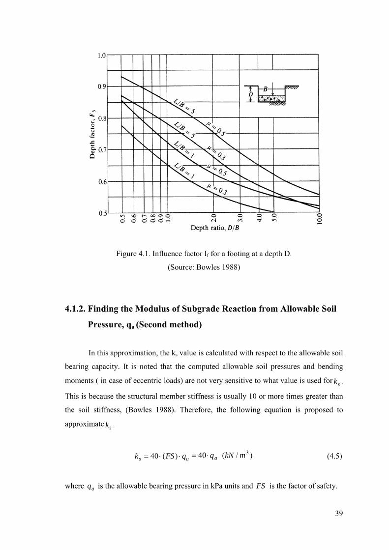
39
Figure 4.1. Influence factor If for a footing at a depth D.
(Source: Bowles 1988)
4.1.2. Finding the Modulus of Subgrade Reaction from Allowable Soil
Pressure, qa (Second method)
In this approximation, the ks value is calculated with respect to the allowable soil
bearing capacity. It is noted that the computed allowable soil pressures and bending
moments ( in case of eccentric loads) are not very sensitive to what value is used for sk .
This is because the structural member stiffness is usually 10 or more times greater than
the soil stiffness, (Bowles 1988). Therefore, the following equation is proposed to
approximate sk .
us qFSk ⋅⋅= )(40 )/(40 3mkNqa⋅= (4.5)
where aq is the allowable bearing pressure in kPa units and FS is the factor of safety.

40
Table 4.1. Values of I1 and I2 to compute the Steinbrenner influence factor
(Source: Bowles 1988)
H/B' L/B = 1, 0 1,1 1,2 1,3 1,4 1,5 1,6 1,7 1,8 1,9 2,00,2 0,009 0,008 0,008 0,008 0,008 0,008 0,007 0,007 0,007 0,007 0,007
0.041 0,042 0,042 0,042 0,042 0,042 0,043 0,043 0,043 0,043 0,0430,4 0,033 0,032 0,031 0,030 0,029 0,028 0,028 0,027 0,027 0,027 0,027
0,066 0,068 0,069 0,070 0,070 0,071 0,071 0,072 0,072 0,073 0,0730,6 0,066 0,064 0,063 0,061 0,060 0,059 0,058 0,057 0,056 0,056 0,055
0,079 0,081 0,083 0,085 0,087 0,088 0,089 0,090 0,091 0,091 0,0920,8 0,104 0,102 0,100 0,098 0,096 0,095 0,093 0,092 0,091 0,090 0,089
0,083 0,087 0,090 0,093 0,095 0,097 0,098 0,100 0,101 0,102 0,1031,0 0,142 0,140 0,138 0,136 0,134 0,132 0,130 0,129 0,127 0,126 0,125
0,083 0,088 0,091 0,095 0,098 0,100 0,102 0,104 0,106 0,108 0,1091,5 0,224 0,224 0,224 0,223 0,222 0,220 0,219 0,217 0,216 0,214 0,213
0,075 0,080 0,084 0,089 0,093 0,096 0,099 0,102 0,105 0,108 0,1102,0 0,285 0,288 0,290 0,292 0,292 0,292 0,292 0,292 0,291 0,290 0,289
0,064 0,069 0,074 0,078 0,083 0,086 0,090 0,094 0,097 0,100 0,1023,0 0,363 0,372 0,379 0,384 0,389 0,393 0,396 0,398 0,400 0,401 0,402
0,048 0,052 0,056 0,060 0,064 0,068 0,071 0,075 0,078 0,081 0,0844,0 0,408 0,421 0,431 0,440 0,448 0,455 0,460 0,465 0,469 0,473 0,476
0,037 0,041 0,044 0,048 0,051 0,054 0,057 0,060 0,063 0,065 0,0695,0 0,437 0,452 0,465 0,477 0,487 0,496 0,503 0,510 0,516 0,522 0,526
0,031 0,034 0,036 0,039 0,042 0,045 0,048 0,050 0,053 0,055 0,0586,0 0,457 0,474 0,489 0,502 0,514 0,524 0,534 0,542 0,550 0,557 0,563
0,026 0,028 0,031 0,033 0,036 0,038 0,040 0,043 0,045 0,047 0,0507,0 0,471 0,490 0,506 0,520 0,533 0,545 0,556 0,566 0,575 0,583 0,590
0,022 0,024 0,027 0,029 0,031 0,033 0,035 0,037 0,039 0,041 0,0438,0 0,482 0,502 0,519 0,534 0,549 0,561 0,573 0,584 0,594 0,602 0,611
0,020 0,022 0,023 0,025 0,027 0,029 0,031 0,033 0,035 0,036 0,0389,0 0,491 0,511 0,529 0,545 0,560 0,574 0,587 0,598 0,609 0,618 0,627
0,017 0,019 0,021 0,023 0,024 0,026 0,028 0,029 0,031 0,033 0,03410,0 0,498 0,519 0,537 0,554 0,570 0..584 0,597 0,610 0.62I 0,631 0,641
0,016 0,017 0,019 0,020 0,022 0,023 0,025 0,027 0,028 0,030 0,03120,0 0,529 0,553 0,575 0,595 0,614 0,631 0,647 0,662 0,677 0,690 0,702
0,008 0,009 0,010 0,010 0,011 0,012 0,013 0,013 0,014 0,015 0,016500,0 0,560 0,587 0,612 0,635 0,656 0,677 0,696 0,714 0,731 0,748 0,763
0,000 0,000 0,000 0,000 0,000 0,000 0,001 0,001 0,001 0,001 0,001
H/B' L/B = 2,5 4,0 5,0 6,0 7,0 8,0 9,0 10,0 25,0 50,0 100,00,2 I1 = 0.007 0,006 0,006 0,006 0,006 0,006 0,006 0,006 0,006 0,006 0,006
I2 = 0.043 0,044 0,044 0,044 0,044 0,044 0,044 0,044 0,044 0,044 0,0440,4 0,026 0,024 0,024 0,024 0,024 0,024 0,024 0,024 0,024 0,024 0,024
0,074 0,075 0,075 0,075 0,076 0,076 0,076 0,076 0,076 0,076 0,0760,6 0,053 0,051 0,050 0,050 0,050 0,049 0,049 0,049 0,049 0,049 0,049
0,094 0,097 0,097 0,098 0,098 0,098 0,098 0,098 0,098 0,098 0,0980,8 0,086 0,082 0,081 0,080 0,080 0,080 0,079 0,079 0,079 0,079 0,079
0,107 0,111 0,112 0,113 0,113 0,113 0,113 0,114 0,114 0,114 0,1141,0 0,121 0,115 0,113 0,112 0,112 0,112 0,111 0,111 0,110 0,110 0,110
0,114 0,120 0,122 0,123 0,123 0,124 0,124 0,124 0,125 0,125 0,1251,5 0,207 0,197 0,194 0,192 0,191 0,190 0,190 0,169 0,188 0,188 0,188
0,118 0,130 0,134 0,136 0,137 0,138 0,138 0,139 0,140 0,140 0,1402,0 0,284 0,271 0,267 0,264 0,262 0,261 0,260 0,259 0,257 0,256 0,256
0,114 0,131 0,136 0,139 0,141 0,143 0,144 0,145 0,147 0,147 0,1483,0 0,402 0,392 0,386 0,382 0,378 0,376 0,374 0,373 0,368 0,367 0,367
0,097 0,122 0,131 0,137 0,141 0,144 0,145 0,147 0,152 0,153 0,1544,0 0,484 0,464 0,479 0,474 0,470 0,466 0,464 0,462 0,453 0,451 0,451
0,082 0,110 0,121 0,129 0,135 0,139 0,142 0,145 0,154 0,155 0,1565,0 0,543 0,554 0,552 0,548 0,543 0,540 0,536 0,534 0,522 0,519 0,519
0,070 0,098 0,111 0,120 0,128 0,133 0,137 0,140 0,154 0,156 0,1576,0 0,585 0,609 0,610 0,608 0,604 0,601 0,598 0,595 0,579 0,576 0,575
0,060 0,087 0,101 0,111 0,120 0,126 0,131 0,135 0,153 0,157 0,1577,0 0,618 0,653 0,658 0,658 0,656 0,653 0,650 0,647 0,628 0,624 0,623
0,053 0,078 0,092 0,103 0,112 0,119 0,125 0,129 0,152 0,157 0,1588,0 0,643 0,688 0,697 0,700 0,700 0,698 0,695 0,692 0,672 0,666 0,665
0,047 0,071 0,084 0,095 0,104 0,112 0,118 0,124 0,151 0,156 0,1589,0 0,663 0,716 0,730 0,736 0,737 0,736 0,735 0,732 0,710 0,704 0,702
0,042 0,064 0,077 0,088 0,097 0,105 0,112 0,118 0,149 0,156 0,15810,0 0,679 0,740 0,758 0,766 0,770 0,770 0,770 0,768 0,745 0,738 0,735
0,038 0,059 0,071 0,082 0,091 0,099 0,106 0,112 0,147 0,156 0,15820,0 0,756 0,856 0,896 0,925 0,945 0,959 0,969 0,977 0,982 0,965 0,957
0,020 0,031 0,039 0,046 0,053 0,059 0,065 0,071 0,124 0,148 0,156500,0 0,832 0,977 1,046 1,102 1,150 1,191 1,227 1,259 1,532 1,721 1,879
0,001 0,001 0,002 0,002 0,002 0,003 0,003 0,003 0,008 0,016 0,031

41
4.1.3. Application of the First and Second Methods in this Study
In this study, sk was calculated by two different approaches, and to stay on the
safe side the smaller one was taken as the sk design value.
1. Estimation of ks by using the first (Es) method;
The modulus of elasticity for silty-sand soils changes between 5 and 20 MPa. In
this study, as the immersed tube is designed with respect to worst conditions, Es was
taken as 5 MPa. In addition, Poisson’s ratio for this type was assumed as 0.35 (Bowles
1988).
The design parameters;
mB 8.39= mL 100= mD 10=
MPaEs 5= 35.0=µ
Corrected sE ′ value is calculated by Eq 4.3:
sE ′sE
)1( 2µ−=
Nm2
76
210755.1
105)35.01( −⋅=
⋅
−=
For the center, H was taken as 1.25B. Because the depth of stress influence
(stress bulb) due to added net foundation pressure, for very large structures is reduced
from 2.5B to 0.75B (Egeli, et al. 1983).
mBH 75.4925.1 =⋅= mBB 9.192==′
5.25.0
25.1'
==BB
BH
→ 343.01 =I from Table 4.1
5.28.39
100==
BL
→ 113.02 =I from Table 4.1.
The settlement influence factor calculated by using Eq 4.4:
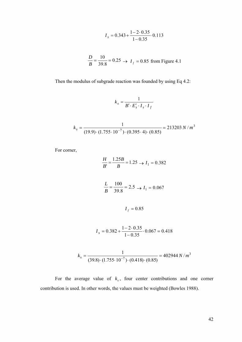
42
113.035.01
35.021343.0 ⋅−⋅−
+=sI
25.08.39
10==
BD
→ 85.0=fI from Figure 4.1
Then the modulus of subgrade reaction was founded by using Eq 4.2:
fsss IIEB
k⋅⋅′⋅′
=1
37 /213203
)85.0()4395.0()10755.1()9.19(1 mNks =
⋅⋅⋅⋅⋅=
−
For corner,
25.125.1'
==B
BBH
→ 382.01 =I
5.28.39
100==
BL
→ 067.01 =I
85.0=fI
418.0067.035.01
35.021382.0 =⋅−⋅−
+=sI
37 /402944
)85.0()418.0()10755.1()8.39(1 mNks =
⋅⋅⋅⋅=
−
For the average value of sk , four center contributions and one corner
contribution is used. In other words, the values must be weighted (Bowles 1988).

43
( )3/251151
54029442132034 mNk avs =
+⋅=
2. Estimation of ks by using the second (qa) method:
The allowable bearing capacity of the soil was calculated in Section 3.1 and had
been found as 0.446 t/m2 (4.374 kN/m2). The modulus of subgrade reaction value is
calculated by Eq 4.5:
as qk ⋅= 40 kN/m3
96.174374.440 =⋅=sk 33 /174960/ mNmkN =
In order to stay on the safe side, the smaller value of the two approaches is used
as the modulus of subgrade reaction of the supporting soil. The results are shown in
Table 4.2.
Table 4.2. The modulus of subgrade reaction (ks) values obtained from 2 different
approaches
The modulus of
subgrade reaction
(ks) (N/m3)
First Method Second Method Used Value
251151.43
174500 174500
4.1.4. Calculation of the Spring Constants
A single tube of 100 m in length is divided into five pieces of 20 m, each. These
pieces are modeled by a mesh of 18 m hexahedral (20 noded) elements. The bottom face
of such a meshed segment that rests can soil is shown in Figure 4.4. The soil is modeled
as linear spring elements, which are connected to the nodes indicated in Figure 4.4. An

44
isoperimetric view of the meshed tube segment, together with the spring element is
shown in Figure 4.2. The spring constants at each node are obtained by the
multiplication of the modulus of subgrade reaction with the area of the face of the
corresponding element and are weighted by a factor, as is shown in Figure 4.3. Thus,
isjj
i kAK α⋅⋅= (4.6)
where; jiK is the spring constant connected to the ith node of the element j, jA is the face
area(that is in contact with soil) of the jth element, and iα is the weighting factor of the
ith node. (See Figure 4.3)
Figure 4.2. The modeling of the tube unit and the elastic foundation in Calculix

45
Figure 4.3. The weights for vertical spring constants corresponding to each node of a
hexahedral element face (Source: Calculix 1.7 2007)
The above figure illustrates the distribution of the Ki value over the element
surface (tunnel unit’s soil base). If an edge or a corner node is shared by more than one
element, the spring stiffness of that node is simply superimposed.
Figure 4.4. The modeling of the elastic foundation of the tube unit.
The areas of the base surface of the tube from Figure 4.3.
216208.07531 mAAAA =×==== (4.7)
1 / 3
1 / 3
1 / 3
1 / 3
- 1 / 1 2 - 1 / 1 2
- 1 / 1 2- 1 / 1 2
20
0.813.80.810.60.813.80.8
A2
A1
A3
A4
A5
A6 A7
ES1,ES3,ES5
ES2,ES4,ES7
ES3,ES6
ES5,ES3,ES10ES8 ES13 ES10,ES3,ES5 ES8 ES5,ES3,ES1
ES3,ES6ES11,ES6ES6,ES11
ES12,ES4,ES5
ES14
ES9
ES7,ES4,ES12 ES5,ES4,ES2

46
2260201362 mAA =×== (4.8)
2212206.104 mA =×= (4.9)
Considering the meshing model, 13 different vertical spring constants were
calculated by using Eq 4.6.
( ) -233333)16()175000(12/11 =⋅⋅−=ES mN / (4.6.a)
( ) -233333)16()175000(12/12 =⋅⋅−=ES mN / (4.6.b)
( ) 933333)16()175000(3/13 =⋅⋅=ES mN / (4.6.c)
( ) 933333)16()175000(3/14 =⋅⋅=ES mN / (4.6.d)
( ) -40250001)260()175000(12/15 =+⋅⋅−= ESES mN / (4.6.e)
( ) 161000003)260()175000(3/16 =+⋅⋅= ESES mN / (4.6.f)
( ) -40250001)260()175000(12/17 =+⋅⋅−= ESES mN / (4.6.g)
( ) 15166667)260()175000(3/18 =⋅⋅=ES mN / (4.6.h)
( ) 15166667)260()175000(3/19 =⋅⋅=ES mN / (4.6.i)
( ) mNESES /33250001)212()175000(12/110 −=+⋅⋅−= (4.6.j)
( ) 133000003)212()175000(3/111 =+⋅⋅= ESES mN / (4.6.k)
( ) mNESES /33250001)212()175000(12/112 −=+⋅⋅−= (4.6.l)

47
( ) 12366667)212()175000(3/113 =⋅⋅=ES mN / (4.6.m)
( ) 12366667)212()175000(3/113 =⋅⋅=ES mN / (4.6.n)
4.2. Static Analysis of the Tunnel for Worst Case Scenario
Tunnel units are built at the shore and below the sea level. The construction
procedure of each tube unit undergoes four basic steps:
i) Construction at land,
ii) Coverage of its open ends, so that it floats on water, and can be pulled to its
position
iii) It is slowly lowered down to the seabed by allowing water to drain into the
tube. Positioning is accomplished by using steel cables, GPS and divers.
iv) Finally, the sides are filled with sand and gravel in a slurry form with the
help of pumps.
The aim here is to investigate the amount of subsoil settlement when the water-
filled tube with water is placed upon it. If the settlement value of the subsoil is bigger
than the tolerable settlement value (2.5 cm), the subsoil needs to be improved.
The static analysis was made only for the tube placed to the dredged trench
location with the greatest depth of seawater (17.5 m). Hence, there was no need for
another analysis, because it was assumed that the elastic properties of the tunnel seabed
soil are the same along the tunnel route; since a limited borehole data was available (the
worst borehole data in Çiğli side was used in the analysis). Moreover, the effective
pressure on the subsoil is the same during immersion of each tube unit. Therefore, there
was no need to make displacement (i.e. settlement) analysis for each tube unit. The
Calculix model of the tube that was illustrated in Figure 4.2 consists of a mesh with
twenty noded brick elements (C3D20) (see Figure 4.5) and the elastic foundation was
assembled with two noded linear spring elements. Each tube unit model consists of 90
C3D20 elements and 130-spring elements. Boundary conditions were applied such that
only vertical motion was allowed. Only the base of the springs was fixed in all
directions. In addition, it was assumed that the side fills had no effect on the vertical
motion of the tube under its gravity loads. Pressures acting on to the subsoil (as soon as
the water-filled tube with water is placed upon it) are illustrated in Figure 4.6 and

48
calculated as below. The displacement analysis should be carried out for the worst case
(maximum loading on the soil). Two scenarios can be considered: One during the
placement of the tube, another during service failure.
1. If no problem occurs during immersion process of the tubes, there will be no
excessive loads acting onto the seabed. However, in the design phase, a worst-case
scenario must be considered. Water leakage, and hence a tunnel unit that is completely
filled with water is an undesirable, but possible stage during construction. Therefore,
this analysis case consists of a tunnel unit being placed onto its seabed, its top covered
with an extra protective material layer, and the inside of the tunnel being filled with
water.
2. When the tunnel is in service, the additional loads come from the sidewalks
and the traffic, only. Here, the worst-case scenario is the tube filled with cars, trucks,
trains, and water due to a water leakage in the joints.
The failure scenario described in item number two will result in larger pressure
acting on the subsoil. Therefore, only one analysis will suffice to find the maximum
displacement.
Figure 4.5.Twenty-noded brick element (C3D20) in Calculix
(Source: Calculix 1.7 2007)
13
124
18
620
14
1117
5
168 15 7
19
3
10
91 2

49
a) Pressure transferring on the b) Pressure transferring on the seabed soil after
seabed soil before dredging dredging
Figure 4.6. The foundation pressure on the seabed soil before and after construction of
the IBITT
4.2.1 Total Pressure Transferred to the Seabed Soil
a) Checking the floatability during transportation of the empty tunnel unit to its
dredged location:
The total width of the tunnel is 39.8 m, and height is 10 m. The widths of the
highways are 13 m and height is 6.7 m, and the width of the railway is 10.6 m, and the
height is 6.7 m. The length of the tube is 100 m. The density of reinforced concrete is
2.5 t/m3 and seawater is 1.027 t/m3.
Subtracting the volumes of each hole from the total volume of the tube, the
concrete volume of the tube could be calculated.
( ) ( ) ( ) ( ) 3152781007.6131007.66.101007.613101008.39 mVnet =××−××−××−××= (2.1)
BEFORE AFTER
water+traffic
1 m
10 m
17.5
m
2Phidrostatik=29.27 t/m2Phidrostatik=29.27 t/m
2 P3 = 36.78 t/m
2 P2= 20.32 t/m
2 P1= 17.97 t/m
P0 = 0 t/m2
2
2
2
P3 = 35.6 t/m
P2 = 19.6 t/m
P1= 17.97 t/m
2 P0 = 0 t/m

50
If the density of concrete is multiplied by the concrete volume of the tube, the
total weight of the tube will be found:
tWtube 38195)5.215278( =×= (2.2)
The natural buoyancy of water applied from foundation level to sea level:
tF buoyancy 40874027.1)100108.39( =×××= (2.3)
tubebuoyancy WF > → The tube floats, which is O.K.
b) Checking the sinkability of the tunnel unit during lowering to its dredged
location:
The unit weight of the armor stone per square m.:
2/30.16.25.0 mtParmorstone =×= (2.4)
The unit weight of the sand-concrete per square m.:
2/05.11.25.0 mtP concretesand =×=− (2.5)
The pressure on the seabed soil due to the water layer on the tube:
2/97.17027.15.17 mtP positivewater =×=− (2.6)
To sink the tunnel element, there is no need to completely fill it with water. A
water depth of 1 m inside the tube is sufficient.
tW ubewater 3759027.1))10016.10()1000.113(2(int_ =×××+×××= (2.7)
Thus, the weight of the 1m water filled tunnel unit is:

51
tWWW watertubetubesemifilled 41954375938195_ =+=+= (2.8)
buoyancytubedsemifiille FW >_ → The tunnel element sinks to its dredged location.
However, as it is mentioned in Section 4.2. to be prepared for the worst case
conditions, the maximum settlement calculation should be made considering the tunnel
is in service and due to a water leakage it is full filled with water. (Scenario 2, see page
49).
The weight of the fully filled tube is calculated as below:
tW tubedwaterfille 63379027.1))1007.66.10()1007.6132((39800_ =×××+×××+=
(2.9)
The unit weight of the full-filled tube is calculated as below:
2/92.151008.39
63379 mtP dtubewaterfille =×
= (2.10)
The weight of the traffic loads is calculated as below. The train load is
calculated according to S (1950) Freight Train from “Alman Federal Demiryolları-Çelik
Demiryol Köprüleri için Hesap Esasları (BE)”technical code. The Figure… shows the
distribution of the loads in S (1950) Freight Train.
Figure 4.7. S (1950) load train
(Source: Alman Federal Demiryolları-Çelik Demiryol Köprüleri için Hesap
Esasları (BE) )
P2=8 t/m
P1=10 t/m
w2<325 mw1=40 m
5x25 t
5x1.6 m

52
tW trainloading 1882)8524.1040255(2 =×+×+××= (2.11)
There are 3 line in highway and it is assumed that max. 25 cars can be placed in
a line and the weight of the car with people is 1.9 tons can be assumed.
tWcar 285)9.1325(2 =×××= (2.12)
The pressure occurring due to the traffic effect can be calculated as below:
2/54.0
)1008.39()2851882( mtPtraffic =
×+
= (2.13)
The total pressure transferred to the soil is calculated:
negativewatertrafficlayerprotectivepositivewaterfilledtubetotal PPPPPP −− −+++= (2.14)
2/51.7)027.15.28(54.0)30.105.1(97.1792.15 mtPtotal =×−++++=
The net effective soil stress at the dredged foundation level of the tunnel, which
is 11 m below of the seabed soil:
2/30.6)027.16.1(11 mtPsoil =−×= (2.15)
Subtracting the permanent total pressure transferred to the soil from the net
effective soil stress at the dredged foundation level, the net effective stress increase can
be calculated as below:
2/21.130.651.7 mtP veneteffecti =−=′ (2.16)
Due to the increase of the net effective pressure on the seabed soil, the vertical
displacement of the tunnel was calculated as 6.59 cm but this value is above the
permissible settlement value of 2.5 cm for each immersed tube unit. The permissible

53
settlement value is a serviceability requirement for tunnels and immersed tube tunnels
containing railroads and highways, designed and constructed in the Far East (Egeli
1996). At first glance, it might appear reasonable to decrease the tunnel dimensions, in
order to decrease the stress on the subsoil. Nevertheless, no matter what dimensions are
used, settlement value is likely to be exceeded.
Also, remember that the mass is necessary to overcome the buoyancy (lift)
forces of the water. Thus, dimensions cannot be decreased. To overcome this drawback,
compaction grouting type ground improvement is suggested for the seabed soil.
Moreover, this is a good precaution against the seismic forces risk and overcoming its
induced further settlement. (See Chapter 5). The static analysis result in Calculix is
shown in Figure 4.8.
Figure 4.8. Maximum vertical displacement of the tunnel

54
CHAPTER 5
SEISMIC ANALYSIS OF THE IMMERSED TUBE
TUNNEL
It is principally recognized that underground structures is affected less from
earthquakes than buildings on the ground surface (Kouretzis, et al. 2006). Therefore, in
the past, most tunnel structures were designed and built without regard to seismic
effects (Taylor, et al. 2005). A seismic design procedure was applied to a tunnel project
for the first time in the 1960s by civil engineers for immersed tube tunnel; The Deas
Tunnel is the first project that is designed taking the earthquake effects into
consideration (Wang 1993, Grantz, et al.1993). For instance, the Bay Area Rapid
Transit (BART) tunnel in San Francisco, California and Osaka South Port (OSP)
immersed tube tunnel in Japan have been subjected to strong seismic shaking.
Nevertheless, since these tunnels had been designed considering the seismic effects,
both tunnels behaved exceptionally well, by sustaining no measurable damage
(Anastasopoulos, et al. 2007). On the other hand, the Alameda Tubes in the San
Francisco Bay Area, which were some of the earliest immersed tube tunnels built in
1927 and 1963, were designed without any seismic design considerations. Therefore,
during the Loma Prietta Earthquake (1989), some cracking was experienced in the
ventilation buildings and limited water leakage into the tunnels was observed. (Hashash,
et al. 2001).
The purpose of this chapter was to develop a pre-seismic design of the immersed
tube tunnel in order to give the structure the capacity to withstand the loads or
deformations/displacements applied to it during an earthquake. A seismic design should
cover all components of the tunnel including, portal buildings, ventilation buildings,
approach structures etc. However, in this study only the immersed tube units, the joints
of the tube units and the elastic foundation underneath were considered.

55
5.1. Types of Deformations
The response of tunnels to seismic shaking motions was explained below (Wang
1993):
1. Axial and Lateral Deformations: Axial and lateral deformations develop in
a linear tunnel, when seismic waves propagate either parallel or oblique to the tunnel.
The tunnel lining considerations for these types of deformations are in the tunnel
longitudinal direction along the tunnel axis. The idealized representations of axial and
lateral deformations are illustrated in Figure 5.1. Vertical deformations are also present
during an earthquake. These are less detrimental, because the vertical stiffness of the
tube only one tenth of its lateral stiffness. Therefore, vertical deformations are not
considered in the analysis.
2. Ovaling (for circular tunnels) or racking (for rectangular tunnels): Since
the dimensions of a typical lining cross-section of the tunnel are small compared with
the earthquake wavelengths, the ground motions produce racking effect (Penzien 2000).
Ovaling or racking deformations may develop in tunnel structures, when waves
propagate in a direction perpendicular or nearly perpendicular to the tunnel axis,
resulting in a distortion of the cross-sectional shape of the tunnel lining (Wang 1993).
The racking deformation of the rectangular tunnel section is shown in Figure 5.2.
5.2. Seismic Analysis Procedures
The seismic design of underground structures differs from the design of surface
structures. Surface structures are not only directly subjected to the excitations of the
ground. They experience amplification of the shaking motions depending on their own
vibratory characteristics. Underground structures, on the other hand, are constrained by
the surrounding medium. Hence, they can not progress to a considerable amount of
deformation, independently from the medium nor can they be subjected to a vibration
amplification (Wang 1993).

56
Figure 5.1. Axial and lateral deformations along a tunnel
(Source: Wang 1993)
Figure 5.2. Racking deformation of a rectangular tunnel
(Source: Wang 1993)
Tunnel Axis
Tension Compression
A. Axial deformation along the tunnel (top view of the tunnel)
NegativeCurvature
PositiveCurvature
B. Curvature deformation along the tunnel (top view of the tunnel)
Tunnel Axis
Tunnel DuringW ave M otion
Tunnel BeforeW ave M otion
Shear W ave Front

57
5.2.1. Free-Field Deformation Approaches
The term ‘free-field deformation’ describes ground strains caused by seismic
waves in the absence of structures or excavation. In this approach, the interaction
between the underground structure and the surrounding ground is ignored.
The free-field deformation method provides a simple and effective design, if the
ground is very stiff and has low shaking intensity or the structure is more flexible than
the surrounding medium. For soft soils (the structure is stiffer than the medium), this
approach provides a first-order estimate of the anticipated structural deformation
(Hashash, et al. 2001). The axial and lateral deformation of the tunnel lining by using a
free field deformation approach can be estimated by using a structural analysis program
or by a hand calculation. The strains of the tunnel due to the seismic wave propagation
according to the simplified procedure are explained below.
5.2.1.1. Closed Form Solution Method (Simplified Procedure)
For practical purposes, Newmark developed a simplified approach in 1968. This
method is one of the free-field deformation approaches. According to this method, the
structure and the ground in the free field experience the same strains (Wang 1993).
Figure 5.3 shows free-field ground deformation along a tunnel axis due to a sinusoidal
shear wave with a wavelength, L, a displacement amplitude, D, and an angle of
incidence, a. The axial and lateral deformations of the ground and the shear (racking)
deformation of the tunnel, due to the shear wave is calculated by using Eq 5.1 and 5.3,
respectively.
The axial (longitudinal) strain;
aaCV
s
s cossin ⋅⋅=ε (5.1)
The lateral;
aCA
r s
s 32 cos1
⋅=⎟⎠⎞
⎜⎝⎛ (5.2)
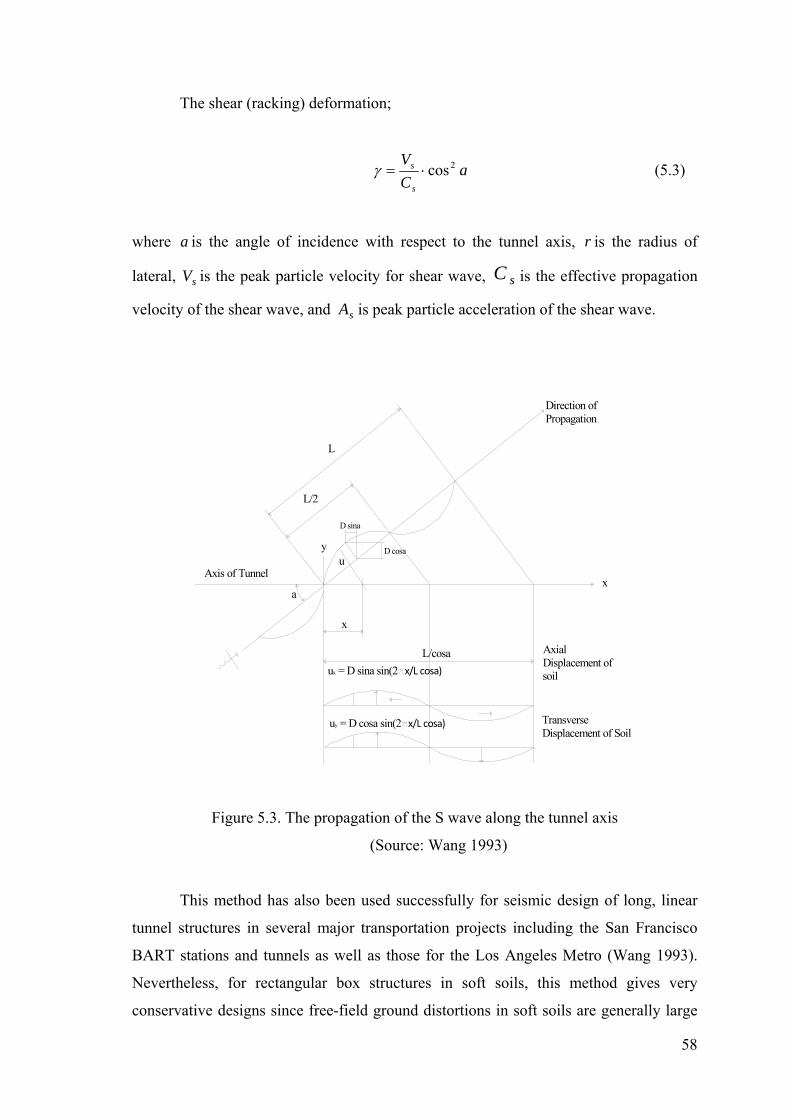
58
The shear (racking) deformation;
aCV
s
s 2cos⋅=γ (5.3)
where a is the angle of incidence with respect to the tunnel axis, r is the radius of
lateral, sV is the peak particle velocity for shear wave, sC is the effective propagation
velocity of the shear wave, and sA is peak particle acceleration of the shear wave.
Axis of Tunnelx
L
L/2
D sina
D cosau
y
x
L/cosa
Direction ofPropagation
AxialDisplacement ofsoil
TransverseDisplacement of Soil
ux = D sina sin(2 x/L cosa)
uy = D cosa sin(2 x/L cosa)
a
Figure 5.3. The propagation of the S wave along the tunnel axis
(Source: Wang 1993)
This method has also been used successfully for seismic design of long, linear
tunnel structures in several major transportation projects including the San Francisco
BART stations and tunnels as well as those for the Los Angeles Metro (Wang 1993).
Nevertheless, for rectangular box structures in soft soils, this method gives very
conservative designs since free-field ground distortions in soft soils are generally large
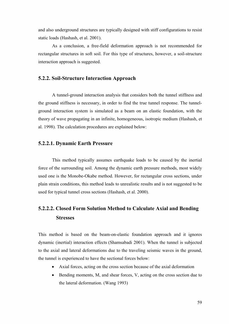
59
and also underground structures are typically designed with stiff configurations to resist
static loads (Hashash, et al. 2001).
As a conclusion, a free-field deformation approach is not recommended for
rectangular structures in soft soil. For this type of structures, however, a soil-structure
interaction approach is suggested.
5.2.2. Soil-Structure Interaction Approach
A tunnel-ground interaction analysis that considers both the tunnel stiffness and
the ground stiffness is necessary, in order to find the true tunnel response. The tunnel-
ground interaction system is simulated as a beam on an elastic foundation, with the
theory of wave propagating in an infinite, homogeneous, isotropic medium (Hashash, et
al. 1998). The calculation procedures are explained below:
5.2.2.1. Dynamic Earth Pressure
This method typically assumes earthquake loads to be caused by the inertial
force of the surrounding soil. Among the dynamic earth pressure methods, most widely
used one is the Monobe-Okabe method. However, for rectangular cross sections, under
plain strain conditions, this method leads to unrealistic results and is not suggested to be
used for typical tunnel cross sections (Hashash, et al. 2000).
5.2.2.2. Closed Form Solution Method to Calculate Axial and Bending
Stresses
This method is based on the beam-on-elastic foundation approach and it ignores
dynamic (inertial) interaction effects (Shamsabadi 2001). When the tunnel is subjected
to the axial and lateral deformations due to the traveling seismic waves in the ground,
the tunnel is experienced to have the sectional forces below:
• Axial forces, acting on the cross section because of the axial deformation
• Bending moments, M, and shear forces, V, acting on the cross section due to
the lateral deformation. (Wang 1993)

60
Simplified Interaction Equations:
The axial forces caused by a shear wave with 45 degree angle of incidence can
be obtained from:
a
cc
a
a
DL
AEK
LK
Q 2max
221
2
⎟⎠⎞
⎜⎝⎛⎟⎟⎠
⎞⎜⎜⎝
⎛+
=
π
π (5.4)
where, L is the wavelength of an ideal sinusoidal shear wave, aK is the longitudinal
spring coefficient of medium in force per unit deformation per unit length of tunnel,
aD is the free-field displacement response amplitude of an ideal sinusoidal shear wave,
cE is the modulus of elasticity of tunnel lining, and cA is the cross-section area of tunnel
lining.
The maximum axial strain can be obtained from the equation below:
cc
axial AEQ⋅
= maxε (5.5)
b
cc
t
t
DL
IEK
LKM 4
2
max
21
2
⎟⎠⎞
⎜⎝⎛⎟⎟⎠
⎞⎜⎜⎝
⎛+
⎟⎠⎞
⎜⎝⎛
=
π
π (5.6)
where, cI is the moment of inertia of the tunnel section, tK is the transverse spring
coefficient of medium in force per unit deformation per unit length of tunnel, bD is the
free-field displacement response amplitude of an ideal sinusoidal shear wave.
Once the maximum bending moment is found by Eq 5.6, the corresponding
stress at the tunnel sides are evaluated as follows:
cI
BM )2/(maxmax
⋅=σ (5.7)

61
The maximum bending strain is calculated from the equation below:
cc
bending IEBM
⋅⋅
=)2/(maxε (5.8)
The maximum shear force corresponding to the maximum bending moment is
derived as:
L
MV π2maxmax ⋅= (5.9)
Once the design parameters are found, they should be checked against the
allowable values. For concrete, the allowable shear strength is calculated by the formula
given below:
shearcdc AfV ⋅⋅= 22.0 (5.10)
The maximum strain should be less than the allowable strain:
bendingaxial εεε +=max allowableε≤ (5.11)
where allowableε is the allowable tensile strain of the concrete. In the equations above,
aK and tK are different from the conventional beam on elastic foundation problems,
since the spring coefficients should be representative of the dynamic modulus of the
ground under seismic loads. In addition, the derivations should consider the fact that
loading felt by the surrounding soil (medium) is alternately positive and negative due to
an assumed sinusoidal seismic wave. For a preliminary design, the expression suggested
by St. John and Zahrah (1987) should serve the purpose:
LHG
KKs
ssat ⋅
−−⋅
==)3(
)1(16ν
νπ (5.12)

62
where, sG is the shear modulus of the medium, sν is the poison’s ratio of the medium,
H is the height of a rectangular structure (or diameter of a circular tunnel), and L is the
wavelength.
The wavelength is not known, but it can be estimated by using the shear wave
velocity.
sCTL ⋅= (5.13)
where, the predominant natural period, T , can be estimated from the soil deposit at a
tunnel site (Wang 1993):
s
s
CH
T4
= (5.14)
where, sH is the soil deposit thickness over rigid bedrock and sC is the shear wave
velocity of the medium.
5.2.2.3. Numerical Analysis Method to Calculate Axial and Bending
Stresses
Another method to determine the displacements and stresses developing in the tunnel’s
longitudinal direction during a seismic activity is by using numerical methods. The
numerical analysis of underground structures can be made by using either lumped
mass/stiffness methods or by finite element/difference methods (Hashash, et al. 2001).
5.2.2.4. Closed Form Solution Method to Calculate Racking
Deformations
Rectangular tunnels are usually built in shallow soils and design of such tunnels
requires careful consideration of soil structure interaction analysis for two reasons:

63
1. There is a larger deformation during an earthquake in shallow soils than in
deeper soils, because of the decreased stiffness of the surrounding soils, due to a lower
overburden pressure. Thus, the site amplification effect is high.
2. Rectangular tunnel linings are usually built stiffer than circular tunnel linings
in their transverse direction and hence, they are less tolerant to deformations (Husam, et
al. 2005).
Then, the racking deformation of a tunnel was calculated by using two different
approaches:
1. Simple Frame Analysis Model: In this approach, only the tube unit is
modeled without the surrounding soil under simple boundary conditions, as shown in
Figure 5.6. This approach should be used for a first-order estimate, although
conservative results can be obtained. The simplicity of the modeling makes the analysis
worthwhile and gives a relationship between the shear deformation flexibilities of the
tunnel and the soil.
The procedure to calculate the racking deformation in rectangular tunnels is
defined below (Wang 1993):
Firstly, the earthquake design parameters should be determined, including at
least the magnitude of the earthquake, peak ground accelerations, amax (Zt), and Cs,
according to level earthquake parameters, which are Type I (severe) earthquake and
Type II (moderate) earthquake. Then, based on the soil properties and the design
earthquake parameters, the free-field shear strains/deformations of the ground are
determined.
s
ss C
V=γ (5.15)
svs aRV ⋅= (5.16)
where, vR is the ratio of peak ground velocity to peak ground acceleration and
determined from Table 5.2., sa is the peak particle acceleration associated with S waves
and found from the formula below:
maxaRa as ⋅= (5.17)

64
in here, aR is the ratio of the ground motion at the tunnel base depth to the motion at the
ground surface and is determined from Table 5.1, and maxa (Zt) is the peak ground
acceleration, determined from Table 3.3.
Then, the free-field deformation is calculated by Eq 5.18:
Hsfieldfree ⋅=∆ − γ (5.18)
where, H is the height of the structure
Table 5.1. Ratios of ground motion at the tunnel foundation (base) level to the motion at
the ground surface (Source: Power, et al. 1996).
Tunnel depth (m)
Ratio of the ground motion at tunnel
foundation level to motion at the ground
surface
6≤ 1.0
6-15 0.9
15-30 0.8

65
Table 5.2. Ratios of peak ground velocity to peak ground acceleration at the surface in
rock and soil (Source: Power, et al. 1996).
Moment
Magnitude(Mw)
Ratio of peak ground velocity (cm/s) to peak
ground acceleration (g)
Source-to-site distance (km)
0-20 20-50 50-100
Rocka
6.5 66 76 86
7.5 96 97 109
8.5 127 140 152
Stiff Soila
6.5 94 102 109
7.5 140 127 155
8.5 180 188 193
Soft Soil
6.5 140 132 142
7.5 208 165 201
8.5 269 244 251
Note: a in this table, the sediment types represent the following shear wave velocity
ranges: rock ≥ 750 m/s; stiff soil 200-750 m/s; and soft soil <200 m/s. The relationship
between peak ground velocity and peak ground acceleration is less certain in soft soils.
The relative stiffness (flexibility ratio) is derived from the expressions below:
The angular distortion of a soil when subjected to shear strain is calculated by
Eq 5.19:
HG
fieldfree
ss
−∆==
τγ (5.19)

66
After rearranging this equation, the shear or flexural stiffness of the tunnel
element can be written as the ratio of the shear stress to a corresponding angular
distortion:
ss
GH
=∆
=)(
τγτ
(5.20)
A distributed force, P , is applied along the tube length to the top of the structure,
acting in the transverse direction (Figure 5.4). The resulting lateral displacement,∆ , is
calculated by a structural analysis program. Once the displacement,∆ , corresponding to
the applied force, P , is obtained, a linear relationship between the two can be written as
follows:
∆⋅= 1SP (5.21)
where, 1S is the force per length that is required to cause a unit racking deflection of the
structure.
The applied shear stress can also be converted into a concentrated force, P , by
multiplying it by the width of the structure (B) and its unit length, resulting in the
following expression for angular distortion:
11
1SH
BSH
PHs ⋅
⋅⋅=
⋅=
∆=
τγ (5.22)
Combining Eq 5.19 and Eq 5.22, the flexibility ratio of the structure can be
calculated as follows:
soilsstructures γγ =
s
soilstr
GSHB ττ
=⋅⋅⋅
1
1

67
1
1SHBG
F s
structure
soil
⋅⋅⋅
==ττ
HSBG
F s
⋅⋅
=1
(5.23)
where sG is the shear modulus of soil, H is the height of the structure, and B is the
width of the structure.
The shear modulus can be calculated as follows:
2ss CG ⋅= ρ (5.24)
where ρ is the density of the saturated soil
In this expression, the unit racking stiffness is the reciprocal of the lateral racking
deflection, 11 /1 ∆=S caused by a unit concentrated force. It can be obtained from
simple static analysis of the box structure, without including the surrounding soil but
under simple boundary condition, as shown in Figure 5.4 (Ostadan and Penzien 2001).
Figure5.4. The racking deflection of the tunnel when applying unit displacement
sideway (Source:Wang 1993)

68
The flexibility ratio gives an idea about the response of the structure and the
surrounding medium (Wang 1993):
F→0.0: The structure is rigid, so it will not rack regardless of the distortion of
the ground (i.e. the structure must take the entire load)
F<1.0: The structure is considered stiff relative to the medium and will therefore
deform less
F=1.0: The structure and medium have equal stiffness, so the structure will
undergo approximately free-field distortions.
F>1.0: The racking distortion of the structure is amplified relative to the free
field, though not because of dynamic amplification. Instead, the distortion is amplified
because the medium now has a cavity, providing lower shear stiffness than non-
perforated ground in the free field.
F ∞→ : The structure has no stiffness; soil will undergo deformations identical
to the perforated ground.
Based on the flexibility ratio, the racking coefficient R defined as the normalized
structure racking distortion with respect to the free-field ground distortion can be
estimated from Figure 5.5.
fieldfree
s
fieldfree
s
fieldfree
s
H
HR−−− ∆
∆=
⎟⎟⎠
⎞⎜⎜⎝
⎛ ∆
⎟⎠⎞
⎜⎝⎛ ∆
==γ
γ (5.25)
where, sγ is the angular distortion of the structure, s∆ is the lateral racking deformation
of the structure, fieldfree−γ is the shear distortion/strain of the free-field, and fieldfree−∆ is
the lateral shear deformation of the free-field.
After determining the racking coefficient, the lateral racking deformation of the
structure is calculated by multiplying it by the free-field deformation as below:
fieldfrees R −∆⋅=∆ (5.26)
Then, the stresses in the tunnel section are determined by performing a structural
analysis with an applied racking deformation is shown in Figure 5.6.

69
0.0
0.5
1.0
1.5
2.0
2.5
3.0
0 1 2 3 4 5 6 7 8 9 10
Structure Deform
ation
Poisson Ratio 0.4
Free-Fluid Deform
ation
Poisson Ratio 0.5
Flexibility Ratio F
R=
Note: Triangular symbols: For rectangular tunnels
Solid Lines: For circular tunnels
Figure 5.5. Normalized structure deflections, circular versus rectangular tunnels
(Source: Wang 1993)
Figure 5.6. Simplified frame analysis model
(Source: Wang 1993)
2. The Soil-Structure Interaction Approach: Both the subsoil and the
surrounding medium are modeled together with the tunnel structure. The free field
displacements are applied as boundary condition to the outer edges of the modeled soil
free-field structure=R.
Pseudo-TriangularDeformation /Pressure Distribution

70
medium. The use of soil-structure interaction is highly recommended, because only a
few assumptions are made in this method. Thus, a more reliable result can be expected.
5.3. Application of the Seismic Design Procedures in This Study
The axial and lateral deformations within the immersed tube tunnel, due to received
seismic waves, were calculated by using the tunnel-ground interaction approach, since
the seabed of the İzmir Bay is very soft. First, it was assumed that the earthquake wave
is applied to the structure in longitudinal direction and the max stresses and
deformations were found. These investigations were made by using both the closed
form solution method (simple hand calculation) and by a numerical analysis (finite
element) method. Assuming that the earthquake wave is applied to the tunnel in the
horizontal direction, the max stress in the tunnel was found. This calculation was made
by using both the simple frame analysis method and the soil-structure interaction
approach. Then the results were compared and results that are more realistic were taken
as the design values in the study.
5.3.1. Calculation of the Axial and Lateral Deformations of the
Immersed Tube Tunnel due to an Expected Seismic Wave Action
In the study, it was assumed that a shear wave propagating at 45 degree (angle
of incidence) to the tunnel axis would create the most critical axial strain within the
tunnel structure. The effective shear wave velocity (Cs) of the ground was taken as 130
m/s. This value is based on the İzmir Metro-Stage 1 Halkapınar-Uçyol Underground
Railway Project. In this design-construction project, it was considered that the shear
wave velocity )( sC , of the İzmir soil changes from 130 m/s to 140 m/s (Tezcan 2007).
Moreover, this )( sC value can be calculated as follows:
331.06.80 NCs ⋅= (5.27)
smCs /12746.80 331.0 =⋅=
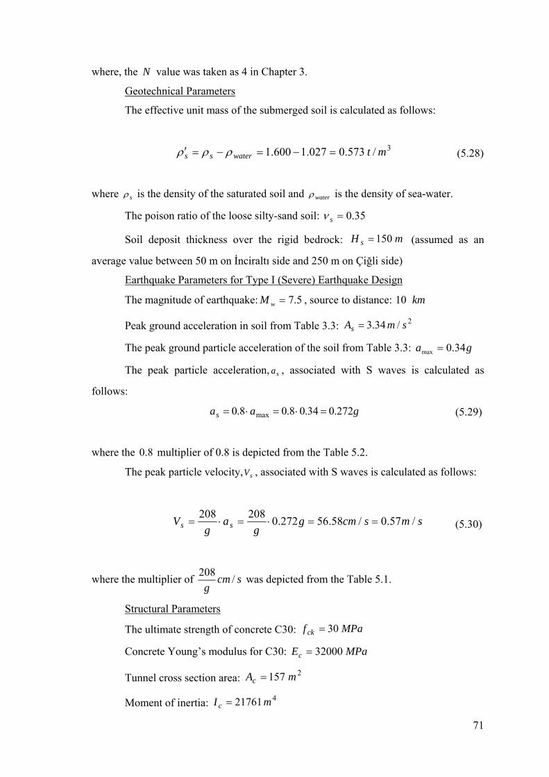
71
where, the N value was taken as 4 in Chapter 3.
Geotechnical Parameters
The effective unit mass of the submerged soil is calculated as follows:
3/573.0027.1600.1 mtwaterss =−=−=′ ρρρ (5.28)
where sρ is the density of the saturated soil and waterρ is the density of sea-water.
The poison ratio of the loose silty-sand soil: 35.0=sν
Soil deposit thickness over the rigid bedrock: mH s 150= (assumed as an
average value between 50 m on İnciraltı side and 250 m on Çiğli side)
Earthquake Parameters for Type I (Severe) Earthquake Design
The magnitude of earthquake: 5.7=wM , source to distance: 10 km
Peak ground acceleration in soil from Table 3.3: 2/34.3 smAs =
The peak ground particle acceleration of the soil from Table 3.3: ga 34.0max =
The peak particle acceleration, sa , associated with S waves is calculated as
follows:
gaas 272.034.08.08.0 max =⋅=⋅= (5.29)
where the 8.0 multiplier of 0.8 is depicted from the Table 5.2.
The peak particle velocity, sV , associated with S waves is calculated as follows:
smscmgg
ag
V ss /57.0/58.56272.0208208==⋅=⋅= (5.30)
where the multiplier of scmg
/208 was depicted from the Table 5.1.
Structural Parameters
The ultimate strength of concrete C30: MPaf ck 30=
Concrete Young’s modulus for C30: MPaEc 32000=
Tunnel cross section area: 2157 mAc =
Moment of inertia: 421761mI c =

72
Width of the tunnel: mB 8.39=
Height of the tunnel: mH 10=
5.3.1.1. Closed Form Solution Method
Using the tunnel-ground interaction procedure
1. The predominant natural period of the soil deposit, T , is estimated by Eq
5.14:
sCH
Ts
s 72.4127
15044=
⋅==
2. The idealized wavelength, L , is estimated by Eq 5.13:
mCTL s 60012772.4 ≅⋅=⋅=
3. The shear modulus of the soil, sG , is calculated by Eq 5.24:
MPamNCG sss 91/90632245127773.0 222 ==⋅=⋅= ρ
4. The equivalent spring coefficients, aK and tK of the soil are calculated by Eq
5.12:
LHG
KKs
ssat ⋅
×−−⋅
==)43(
)1(16ννπ
60010
)35.03()35.01(101.916 7⋅
−−⋅×⋅
=π
mNKK ta /30830069==
5. The ground displacement amplitudes, Da and Db are derived from the
equations below (Newmark 1968):

73
For free field axial strain: LD
CV a
s
s π22
= (5.31)
=⇒ aD π⋅⋅⋅⋅
2127260057.0
aD m214.0=
For free-field bending lateral: 2
23
2
445cos
LD
CA b
s
s π=° (5.32)
22
32
445cos
π⋅
⋅⋅=⇒
s
sb C
LAD
mDb 669.0=
6. Maximum axial force and the corresponding axial strain of the tunnel lining
are calculated.
The maximum axial force, maxQ is calculated by Eq 5.4:
a
cc
a
a
DL
AEK
LK
Q 2max
221
2
⎟⎠⎞
⎜⎝⎛⎟⎟⎠
⎞⎜⎜⎝
⎛+
=
π
π 209.0
2600
157.420 32000000003083006921
260030830069
2 ⋅
⎟⎠⎞
⎜⎝⎛⎟⎠⎞
⎜⎝⎛
⋅⋅+
⋅
=
π
π
NQ 8max 105.68 ×=
The maximum axial strain, axialε , is found from Eq 5.5:
42.15703200000000105.68 8
max
⋅×
=⋅
=cc
axial AEQ
ε

74
00011.0=axialε
7. The maximum bending moment and corresponding bending strain of the
tunnel lining are calculated.
The maximum bending moment, maxM , by using Eq 5.6 is calculated as follows:
b
cc
t
t
DL
IEK
LKM 4
2
max
21
2
⎟⎠⎞
⎜⎝⎛⎟⎟⎠
⎞⎜⎜⎝
⎛+
⎟⎠⎞
⎜⎝⎛
=
π
π 669.0
2600
2176103200000000308300691
260030830069
4
2
⎟⎠⎞
⎜⎝⎛⎟⎠⎞
⎜⎝⎛
⋅+
⎟⎠⎞
⎜⎝⎛⋅
=
π
π
=maxM Nm1010016.4 ×
The maximum bending strain, bendingε , is found from Eq 5.8:
ccbending IE
BM⋅
= ⋅ )2/(maxε5.02176103200000000
5.08.3910072.5 10
⋅⋅⋅⋅
= ⋅
0011.0=bendingε
8. The total strain that may develop during seismic activity is compared with the
allowable strain. The max axial strain, maxε , is found by Eq 5.11:
allowablebendingaxial εεεε ≤+=max
0013.0max =ε ..002.0 KO⇒≤
9. The maximum shear force, dV , due to the bending lateral is calculated by Eq
5.9:

75
600210016.42 10
maxππ
⋅×==L
MVd
NVd810203.4 ×=
10. The allowable shear force, maxV , is found by Eq 5.10:
)(22.0 shearcdc AfV ⋅⋅= 610))47.68.0(157(2022.0 ⋅⋅⋅−⋅⋅=
NVc810423.6 ×=
cd VV < , the shear force does not exceed the allowable shear resistance.
Therefore, the tunnel has enough capacity to resist the shear forces.
11. The maximum bending stress, maxσ , is calculated by using Eq 5.7 as follows:
cIBM )2/(max
max⋅
=σ1.28310
5.08.3910072.5 10 ⋅⋅×=
MPa72.36N/m36723562 2max ==σ
>= MPa72.36maxσ MPafcd 20=
where, cdf is the design compressive strength of C30 concrete.
12. The minimum bending stress, minσ , is calculated by using Eq 5.33 as follows:
cI
BM )2/(minmin
⋅−=σ (5.33)
MPa72.36min =σ (in tension)
Note that (-) sign denotes tensional stress in the tunnel concrete.

76
MPafctd 27.1min =>>σ
where ctdf is the design tensile strength of C30 concrete.
The concrete has not enough capacity to resist the bending stress occurring
during the seismic activity. Therefore, the internal forces must be relieved which can be
accomplished by increasing the flexibility of the structure. Section 5.4 discusses the
seismic analysis after rubber (or neoprene) joints are introduced in between two
adjacent tube unit.
5.3.1.2. Numeric Analysis Method (Finite Element Method)
In this study, the preferred method is the finite element analysis procedure which
is implemented by using SAP 2000, a structural analysis program.
The analysis of the tunnel was performed at a selected mid-route location for a part of
1800 m, of the tunnel which corresponds to three-wave length of the seismic motion of
the soil. A tube unit in 100 m length is divided into 90-cube elements. The model
contains 1926 solid elements and 3456 joints. Since the seabed soil is very loose, in
order to represent the soil-structure interaction, the soil is modelled as well. The seabed
soil is represented by a solid surface springs in SAP 2000. In order to represent
flexibility of the system, elastomeric joints are introduced between two adjacent tube
units. The modulus of elasticity of the elastomeric material used in the model is 3 MPa,
its poison ratio is 0.49, and the length of each elastomeric joint is 0.5 m.
The seismic design loads imposed on the tunnel is defined as displacements. In
other words, the earthquake loads for underground structures are represented in terms of
deformations and strains applied on such structure by the surrounding medium
(Hashash, et al. 2001). Turkey , on the other hand, has no code/standards for design and
construction of tunnels and for immersed tube tunnels in particular as of today. Thus,
the analysis of the system was conducted as an equivalent static analysis and the design
was made for loading condition used in the Far Eastern Projects and defined as below
(Egeli 1996, and Taiwan High Speed Railway Project 2003):
EULLDL 111 ++ (5.34)

77
where DL is the dead load coming from the self weight of the structure, including
material layer and the weight of the water layer above the tube. LL is the live load
coming from the traffic loads and EU is the earthquake displacements (amplitude of the
wave) due to the shear wave. They can be calculated by the formula below:
⎟⎟⎠
⎞⎜⎜⎝
⎛⋅⋅⋅=
)cos/(2sin)(cos
aLx
aDy ii π (5.35)
where D is the amplitude of the wave, a is the angle of the shear wave with
respect to the tunnel longitudinal axis, L is the length of the shear wave and x is the
distance.. In this equation, it was assumed that the amplitude of the shear wave is 1 m
because. It is well known that a maximum probable amplitude value of any shear wave
is assumed as 1 unit. The amplitudes aD and bD of the shear wave of the İzmir Bay was
calculated as 0.214m and 0.669 m. Since, the calculations are made considering worst
case scenario, in this study the amplitude of the shear wave is taken as 1 m. and the
angle of the incidence is 45 degrees. The shear wave is imposed on the structure as
shown in Figure 5.3. Since underground structures are constrained by surrounding
medium and they move together with the ground, the motion of the shear wave is the
same with the tunnel motion during an earthquake. In order to define the motion of the
tunnel during an earthquake, the calculated coordinates in Eq 5.35 are imposed on the
each node of the model in SAP2000 in lateral direction.
First, the analysis was made for the present situation of the seabed soil of the
İzmir Bay. The used modulus of subgrade reaction ( sk ) value was taken as 174500
N/m3 (See Section 4.1.3). As a result of the analysis, the max compressive stress in
longitudinal direction was found as 21x106 N/m2 (21 MPa). It develops on the outer
walls and the top corners of the tunnel, while in lateral direction, the max compressive
stress was found as 45.5 MPa and it develops on the inner walls of the tunnel. The
deformation of the structure during an earthquake is shown in Figure 5.7. The analysis
results are shown in Figures 5.8 and 5.9.

78
Figure 5.7. The deformation of the tube unit during an earthquake.
The analysis shows that the max stress is higher than the design compressive
strength of the concrete (as the used concrete material is C30, fcd=20 MPa). To
eliminate this drawback, ground improvement should be applied to the seabed soil.
Assuming that ground improvement was made and the min SPT_N value rises to 35
after the ground improvement, the new )( sk of the soil is calculated as 5600144 N/m3.
Then, a new analysis was made in SAP2000 by using the same model. As a result of
this analysis, the max compressive stress on the tunnel in both longitudinal direction
and lateral direction was decreased to 19.6x10⁶ N/m2 (19.6 MPa). It is less than the
compressive strength of the C30 concrete. However, the opposite face of the tunnel is
subjected to a tensile stress of the same magnitude (19.6 MPa). This value is
considerably larger than the tensile strength of the concrete (for C30 fctd=1.25 MPa). In
z y
x

79
order to strengthen the structure against tensile stresses, prestressed concrete can be
used (Akan and Özen 2005). The analysis results obtained after ground improvement
are shown in Figures 5.10 and 5.11.
The earthquake design of the tunnel was made by making quastatic analysis in
SAP 2000. In order to apply the SAP2000 modeling procedures, 4 noded solid element
was used and the soil fixed from x, y, and rz (rotation in z dir) axis. Therefore,
conservative stress values were found at the end of analysis. However, the tunnel is
moved together with the surrounding soil during an earthquake, thus the stresses in
lateral direction might be dramatically less than the finding. In addition, since the
elastomer joints are were used, it is probable that less stresses develop on the tubes in
both lateral and longitudinal direction during a seismic motion. Therefore, it is
suggested that in design phase detailed earthquake analysis of the tunnel was made to
obtain results that are more realistic.
Figure 5.8. Max compressive stress on the tube in longitudinal direction (before
ground improvement
max stress in longitudinal direction
21x106 N/m2
zy
x

80
Figure 5.9. Max compressive stress on the tube in lateral direction (before
ground improvement)
Figure 5.10. Max stress on the tube in longitudinal direction (after ground
improvement)
Max stress in lateral direction
45.5x10⁶ N/m2
The max stress in
longitudinal direction
19.6x10⁶ N/m2
z y
x
z y
x
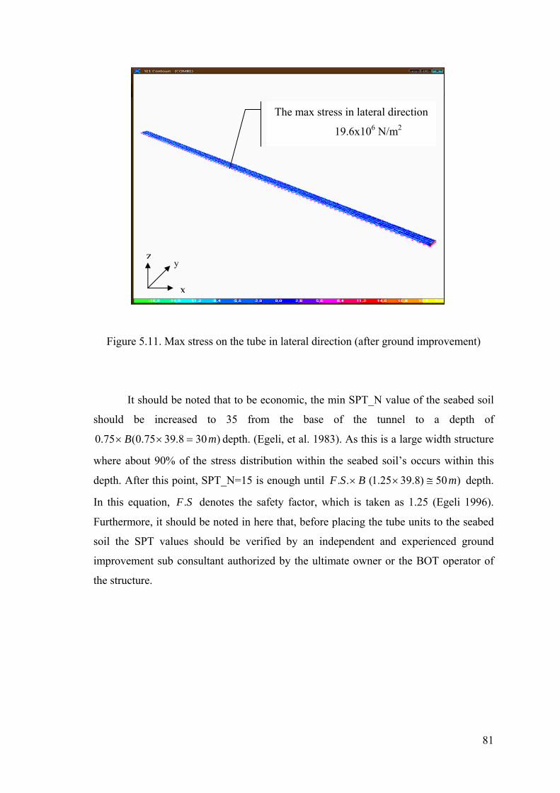
81
Figure 5.11. Max stress on the tube in lateral direction (after ground improvement)
It should be noted that to be economic, the min SPT_N value of the seabed soil
should be increased to 35 from the base of the tunnel to a depth of
)308.3975.0(75.0 mB =×× depth. (Egeli, et al. 1983). As this is a large width structure
where about 90% of the stress distribution within the seabed soil’s occurs within this
depth. After this point, SPT_N=15 is enough until BSF ×.. )50)8.3925.1( m≅× depth.
In this equation, SF. denotes the safety factor, which is taken as 1.25 (Egeli 1996).
Furthermore, it should be noted in here that, before placing the tube units to the seabed
soil the SPT values should be verified by an independent and experienced ground
improvement sub consultant authorized by the ultimate owner or the BOT operator of
the structure.
The max stress in lateral direction
19.6x10⁶ N/m2
z y
x

82
5.3.2. Calculation of Racking Deformation and Stresses of the
Immersed Tube Unit due to an Expected Seismic Wave Action
In this study, the racking deformation of the tube unit was calculated by using
both a simple frame analysis model, and a soil-structure interaction approach. The
results of the two different methods are tabulated for comparison.
5.3.2.1 Simple Frame Analysis Model:
First, the angular distortion of the soil is calculated by Eq 5.15:
0045.0127
57.0===
s
ss C
Vγ
The free-field racking deformation is calculated by Eq 5.18
mHsfieldfree 045.0100045.0 =×=⋅=∆ − γ
The shear modulus of soil is calculated by Eq 5.24
MPamNCG sss 91/90632245127573.0 222 ==⋅=⋅= ρ
The following step is to calculate the force/length per unit displacement, which
is a requirement that causes a unit racking displacement of 1 m. This is accomplished by
modeling a 20 m segment of the tube. The reason why a length of 20 m was used here is
that hour glassing occurred. There was no problem, however, in the results by using 20
noded brick elements over the full length of the model. At the end, the total model
consisted of 18 elements (for the 20 m segment).
S1 is calculated by Eq. 5.21:
289
1 /1011.4)1/()20/1021.8(/ mNPS ×=×=∆=

83
In the equation above, 20 is the length in meters of the length of the tube
segment and 1 is the unit deformation in meters. The deflected shape of the tunnel is
shown in Figure 5.12, and the force variable on the tube unit is illustrated in Figure
5.13.
Figure 5.12. The deformation of the tube unit after applying unit-racking deflection.
The flexibility ratio is calculated by Eq 5.19:
88.0101011.4
8.39906322458
1=
×⋅×
==HSBG
F s
Since, the flexibility ratio is less than one; the structure is stiffer than the
medium and it will not deform as much as the soil.
According to the flexibility ratio, the racking coefficient is determined from
Figure 5.5.
For F=0.88, the racking coefficient is equal to 0.9
The racking deflection is determined by Eq 5.22:

84
mR fieldfrees 04.0045.09.0 =×=∆⋅=∆ −
This means that the racking deformation causes the top of the tube to deflect
0.04 m.
Figure 5.13. Force averaging on the tube unit after applying unit deflection in lateral
direction
This deflection varies linearly over the height of the structure with no
deformation at the base and the max occurs at the top. The resulting stress is found as
9.64x10⁶ N/m2 and it develops upper right-hand corner of the tube. The analysis results
are illustrated in Figures 5.14 and 5.15.

85
Figure 5.14. Maximum racking deflection of the tube unit according to the simple
frame analysis model
Figure 5.15. Maximum Von Misses stress of the tube unit according to simple
frame analysis model
max lateral displacement
0.04 m
max von misses stress
4.62x10⁷ N/m2

86
5.3.2.2. Soil-Structure Interaction Approach
In this approach, a finite element is constructed. The model consists of a 20 m
segment in length of the tube tunnel together with the rock fill at the sides. Quadratic
hexagonal and wedge elements are used to represent the tube and the rocks. The soil,on
the other hand, is modeled by linear axial springs. The spring constants were calculated
by multiplying the modulus of subgrade reaction, ks, with the elements face area, and a
model weighting factor (see Section 4.1.4 for the calculation of spring constants
underneath a hexagonal element).
Figure 5.16. Fifteen noded wedge element in Calculix
(Source:Calculix 1.7 2007)
The racking analysis is performed by applying the free-field deformation to the
outer spring ends. Zero displacement is applied to the depth of 10 m, and
mfieldfree 045.0=∆ − is applied at the top level of the tube. By using this soil-structure
interaction approach, it was calculated that the tubes top surface is displaced by 0.0004
m which causes a Von Misses stress of only 3.37 MPa at the top of the tube. The
analysis results are shown in Figures 5.17 and 5.18.
As it is seen, the results from the simple frame analysis model are much more
conservative than the soil structure interaction approach. This is likely due to the fact
that the simple frame analysis, as the name implies, is simpler and also it is based on a
1012
11
15
839
13
4
65
14
2
71
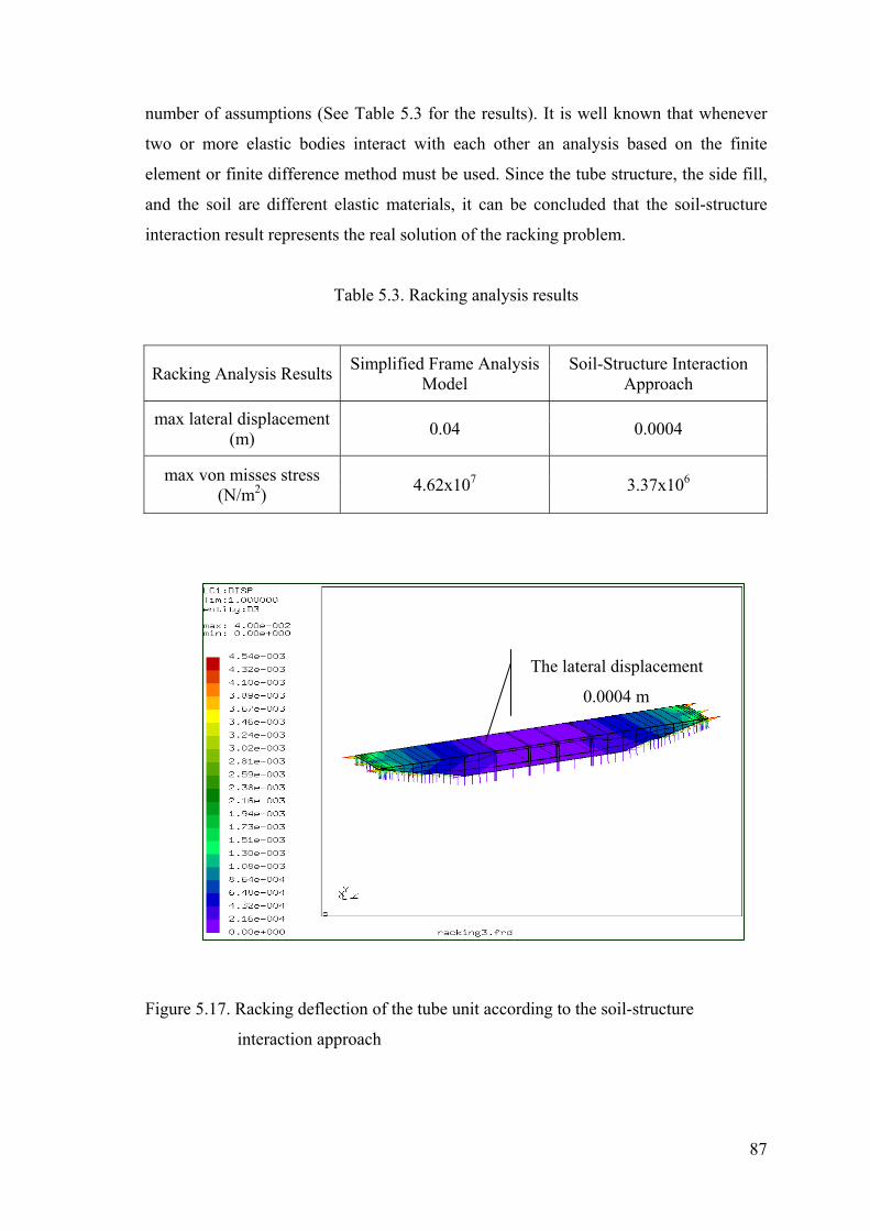
87
number of assumptions (See Table 5.3 for the results). It is well known that whenever
two or more elastic bodies interact with each other an analysis based on the finite
element or finite difference method must be used. Since the tube structure, the side fill,
and the soil are different elastic materials, it can be concluded that the soil-structure
interaction result represents the real solution of the racking problem.
Table 5.3. Racking analysis results
Racking Analysis Results Simplified Frame Analysis Model
Soil-Structure Interaction Approach
max lateral displacement (m) 0.04 0.0004
max von misses stress (N/m2) 4.62x10⁷ 3.37x10⁶
Figure 5.17. Racking deflection of the tube unit according to the soil-structure
interaction approach
The lateral displacement
0.0004 m

88
Figure 5.18. Von misses stress of the tube unit according to simple frame analysis
model
5.4. Seismic Design Issues
The analysis in Section 5.3.1.1 concludes that high stresses develop in the
tunnel, if all tube units are rigidly interconnected. These stresses can be relieved if
elastomer joints are used in between two adjacent tube units. In addition, the tube tunnel
should be made impermeable against water leakage. Hence, flexible joint is
recommended for that reason too (Akimoto, et al. 2002).
Two different joint types are used to connect the adjacent tubes to each other:
a) Conventional Flexible Joint: This type of joint consists of rubber gasket and
connection cables. The cables and gaskets carry tensile and compression forces
respectively at joint parts. The cable-rubber gasket type flexible joint (conventional
flexible joint) which has been especially used for immersed tube tunnels in Japan is
shown in Figure 5.19. Due to possible lateral displacements of the tunnel, large
openings can occur between two adjacent tube units. If large openings occur, they
deteriorate the dewatering performance of the joints. Since, this type of joint cannot
max Von Misses stress
3.37 x10⁶ N/m2

89
provide the dewatering activity between the tunnel elements; a highly flexible joint is
needed to absorb such large displacements (Kiyomiya, et al. 2004).
Figure 5.19. Conventional type flexible joint (Source: Kiyomiya, et al. 2004)
b) Crown Seal Flexible Joint: This type of joint, which consists of a rubber
block, installed at the outside of the bulkhead and flanges connected to the rubber block
and fixed to an attachment plate, is a kind of pin structure. This type of joint shows
excellent performance to absorb the possibly resulting large openings, displacements,
and stresses induced by any seismic effect and by any differential settlement between
the tunnel units. (Kiyomiya, et al. 2004)
Figure 5.20. Crown seal flexible joint ( Source: Akimoto 2002)
Edge of tunnel tube
Secondary cutoff rubber
Cover plate
Nose point
Attachment beam
Buffer rubber
crown seal joint
fitting pointwater pressure
openning

90
5.5. Calculation of Longitudinal Movement between the Two
Immersed Tube Units during an Earthquake
The tube tunnels cannot be rigidly interconnected, because the internal stresses may rise
to such levels that cause structural failure during an earthquake. Therefore, it was
suggested to use flexible joints, which introduce flexibility, and thus reducing the
internal stresses.
The seismic shear waves cause the joints to be compressed in one side of the
tube, and to be extended on the other side. This applies to the right-left, and the top-
bottom sides of the tube interconnections, depending on the seismic wave’s direction
and properties. The top-bottom displacements are less important compared to the right-
left ones, because the tube height is smaller than its width.
The amount of extension and compression for these joints are investigated in
this section for a design specification. In this particular problem, the interconnection of
the adjacent two units at the maximum lateral are considered (units 36 and 37). Figure
5.21 shows an exaggerated layout of these units.
The calculation can be made based on the geometry in Figure 5.21. The y1, y2,
and y3 values are the amplitudes of the earthquake wave at x1, x2, and x3 distances and
they are calculated by Eq 5.33. In addition, θ1, θ3 are the angles between the units and
the tube tunnel alignment, and θ2 is the angle in between the two tube units.
The coordinates x1, x2, and x3 in Figure 5.21 correspond to 3500th (i.e. station
3+500 km), 3600th, and 3700th meters of the immersed tube tunnel.

91
∆x
x xx+100
L=600 m
x-100 x
Figure 5.21. The shape of the immersed tube unit during an earthquake
This means that, the 3500th m. of the immersed tube tunnel is displaced by 0.499
m from the neutral axis during the earthquake (Mw=7.5).
⎟⎟⎠
⎞⎜⎜⎝
⎛⋅⋅⋅=
)45cos/600(36002sin)45(cos12 πy
st
th
36
immers
ed tub
e un
it 37 immersed tube unit
(x2,y2)
(x1,y1)(x3,y3)
LONGITUDINAL TUNNEL AXIS
θ1
θ2
θ3

92
m 0.7062 =y
This indicates that, the 3600th m. of the immersed tube tunnel is displaced by
0.706 m from the neutral axis during the design earthquake (Mw=7.5).
⎟⎟⎠
⎞⎜⎜⎝
⎛⋅⋅⋅=
)45cos/600(37002sin)45(cos13 πy
m 543.03 =y
This shows that, the 3700th m. of the immersed tube tunnel is displaced by 0.543
m from neutral axis during the design earthquake.
In order to calculate the corresponding distortion angles of θ1, θ2, and θ3, the
following relationships are used.
12
121 x-x
y-ytan =θ (5.36)
002.00.002tan 11 =→= θθ
23
233 x-x
y-ytan =θ (5.37)
0.00160.0016tan 33 −=→−= θθ
The angular rotation between the two adjacent immersed tube units is equal
to 2θ . The opening value (the movement of the tube unit in the longitudinal direction)
can be calculated by multiplying the tangent of 2θ by the structure width.
Wopening ⋅=∆ 2tanθ (5.39)
132 θθθ += (5.5.4)
0036.00016.0002.02 =+=θ

93
8.39)0036.0tan( ⋅=∆opening
mopening 14.0=∆
The longitudinal movement between the 36th and 37th tube units of the immersed
tube tunnel is found as 14 cm for the design ground motion. For instance, the axial and
shear displacement of the tube units of the Osaka Port’s Yumeshima Immersed Tube
Tunnel had been investigated in a study, by using both experimental method and the
numerical method during a seismic event. As a result of the study, it was found that the
displacement (opening) of the tube unit changes between 0 to 300 mm in the
longitudinal (axial) direction. Then, it was confirmed that these opening values are
tolerable displacement values and they do not bring about any water leakage during an
earthquake (Kiyomiya, et. al. 2004). Therefore, in order to confirm that the tunnel is
safe against the water leakage and intolerable movements at the time of the designed
seismic action, it should be checked that whether the found displacement (opening)
values calculated for this IBITT are less than the acceptable limits. Also, using the max
moment and shear values occurring due to the design earthquake (Mw=7.5) both in
racking (transverse) and longitudinal direction, concrete crack width checks should be
done to see if they are tolerable and cause no water leakage. As there is no standard
procedure for this check for immersed tube tunnels in Turkey, similar procedure used in
the Far East can be used (Egeli 1996).

94
CHAPTER 6
GROUND IMPROVEMENT ALONG THE TUNNEL
ALIGNMENT
6.1. Ground Improvement
The soil along the tunnel route is very loose and does not enough capacity to
carry the imposed loads due to the tunnel construction. In other words, soil may
undergo large elastic settlements. In such a case, it is necessary to improve the technical
properties of in situ-soil.
To improve the soil, several techniques are available at the present time.
However, choosing of any ground improvement technique depends on the aim of the
ground improvement and the soil type. For instance, since the rock layer has been found
at about 250 m. depth near the Çiğli side, deep foundation technique types (bored piles
socketed into bedrock, friction piles or fibrex piles, and pre-cast piles types friction
piles), ground improvement methods are not applicable for treatment of the tunnel
ground. It is known that precast or vibrex type friction displacement piles in Çiğli side
and Mavişehir sides built in 1980’s continue to settle substantially (Egeli and Pulat
2008) and hence they cannot be considered as reliable foundations in such very deep
and very loose sub-soils. Other vibration techniques such as vibropacement (stone
columns), vibro piles, vibro compaction, and vibro-concrete columns unsuitable for
treatment of the tunnel route subsoil also. Because these methods are suitable to treat
the soil, only up to max 35 m depth from the seabed level.
Grouting which is an alternative ground improvement method can be used for
both rock and soil. Its principle is the injection of liquid materials under pressure into a
soil or rock to change its engineering properties. The following properties can be
improved by the grouting process:
1. Shear strength can be increased.
2. Compressibility, permeability, and liquefaction risk can be reduced.
3. Swelling and shrinking can be controlled.

95
4. Durability can be extended.
There are four types of grouting methods:
1. Chemical (Permeation) Grouting
2. Slurry (Intrusion) Grouting
3. Jet (Replacement) Grouting
4. Compaction (Displacement) Grouting
6.1.1 Grouting Types
1. Chemical Grouting; is done by the injection of a chemically permeable material that
has low viscosity into sandy soil or rock under low pressure. This method is mostly
used for the purpose of controlling water flow and producing sandstone like masses to
carry the imposed loads. As this method is applied under low pressure, engineering
properties of the soil do not change and only its mechanical properties can change, such
as its permeability and porosity. The chemical grouting process is illustrated in Figures
6.1. and 6.2.
Figure 6.1. Chemical grouting process
(Source: Hayward Baker 2008)

96
The chemical (permeation) grouting applications are shown below:
•
•
a) For lagging operation b) Support of footing
c) Grouted tunnel support d) Pit excavation below water
d) Grouted cut-off wall e) Grouted pipeline support
Figure 6.2. Chemical grouting applications
(Source: Hayward Baker 2008)
2. Slurry Grouting; (also called cement grouting) is done by intrusion of a low
viscosity, flowable particulate grout into voids and cracks in a soil, under high pressure.
This grouting is not possible for most of the tunnel-route soils, as N (*) (corrected)

97
values are less than 11. The application process of the slurry grouting process is
illustrated in Figure 6.3.
)()(
85
15
groutDsoilD
N =
where D is the grain size.
Figure 6.3. Slurry grouting process
(Source: Hayward Baker 2008)
Typical slurry (cement) grouting applications are:
• Rock foundation treatment of a dam site
• Rock cut-off curtains
• Pressure injected anchors
• Stabilization of gravels and shotcreted rock
3. Jet Grouting; is a versatile ground modification system used to create in-situ,
cemented formations of soils, called soilcrete. To form soilcrete, the injection pipe is
inserted into the soil at a desired depth. Then the soil is being subjected to a horizontal
high-pressure air water jet, at the same time the soil is mixed with grout, so the
engineering properties of the soil are improved. The most important advantage of this
method is that it can be applied to all soil types. The jet grouting process was shown in
Figure 6.4.

98
Jet grouting applications are:
• Control of underground fluids
• Excavation of unstable soil
Increase the bearing capacity of soil
Figure 6.4. Jet grouting process
(Source: Hayward Baker 2008)
4. Compaction Grouting; is done by injection of a very viscous (low-mobility),
aggregate grout under high pressure to displace and compact the surrounding soil. This
method can be used in any type of soil and underwater, but mostly preferred in soils
finer than the medium sands. One of the most important advantages is that, its
maximum effect is obtained in the weakest soil zones. The compaction grouting process
is shown in Figure 6.5.
Figure 6.5. Compaction Grouting Process
(Source: Hayward Baker 2008)

99
Compaction grouting applications:
• Densification of soil before construction
• Prevention of settlement in tunneling through soft ground
• Provide underpinning of structures
• Strengthen the supporting ground
• Increase the bearing capacity of the founding soils
Decreasing the liquefaction risk of subsoils.
6.2. Encountered Soil Issues of the İzmir Bay
The İzmir Bay seabed consists of very loose to loose silty sands/sandy silts (as
understood from the available 3 borehole data obtained from the DLH) with very low
SPT-N penetration values. Especially, near the Çiğli side, the soil is like a deep swamp
and the penetration values are less than 2. This is why, the soil does not have allowable
bearing capacity to bear the loads transferred to it and causing very large and intolerable
total and differential settlements, underneath the tunnel base. Moreover, the existing
limited subsoil data also shows that the İzmir Bay soil along the IBITT route has high
liquefaction risk, particularly near the Çiğli side. Consequently, it is required to apply a
ground improvement process at the site along the tunnel alignment.
The reasons to make ground improvement are;
• Increase the bearing capacity
• Strengthen the shear strength of the ground
• Decreasing the liquefaction risk
• Decreasing the intolerable settlement
6.2.1 Which Method should be used?
The preferred method for the İzmir Bay is ‘compaction grouting’ type ground
improvement method by virtue of being the most appropriate method, in order to treat
the problems of the seabed soil of İzmir Bay. If four methods are compared, the reason
to choose this method can be understood as below;
Chemical grouting treats the soils’ mechanical properties, such as permeability
and porosity, but it has no effect on the engineering properties of a soil, because of
100
being applied under low pressure. However, the grouting is necessary to improve the
shear strength and settlement properties of the tunnel seabed, as total settlements in
excess of 2.5 cm (25 mm) underneath the tunnel (ie. at the tunnel foundation level) can’t
be tolerated.
Although the slurry method is applied under a high pressure, it is suitable for
rocks and gravels, whose N -values are bigger than 11, but not for loose soils. Though
jet grouting can be used for most soil types, it’s actually not an injection method, but a
kind of mixer technique. Jet grouting mostly used to prevent excessive settlements
beneath the foundations of columns or to form an impermeable barrier against water
leakage for tunnels. In addition, it is still a controversial subject that whether this
method decreases the liquefaction risk of the soil. On top of that, the methods explained
above are not appropriate for using underwater. However, the compaction grouting is
especially used for large areas, including the underwater structures, by virtue of being a
displacement method, it also compacts the soil by displacing it. Because this method is
leads to further compaction of the surrounding soil, the engineering properties of the
soil are also improved. Moreover, it is preferred for liquefiable soils, in order to
diminish this drawback.
Consequently, when all the ground improvement methods are compared, it can
be understood that compaction grouting is the most proper one, in order to meet the
needs of the seabed soils along the tunnel alignment. In addition, if it is investigated, it
can be realized that compaction grouting is a most preferred improvement method for
immersed tube tunnels in the world as well as in the Marmaray Project of our country. It
should be noted that when doing compaction grouting type ground improvement, the
seabed soil area to be treated should be 5 m larger on either side of tunnel base. (i.e
mm 50528.39 =×+ ) due to the stress bulb extension at depth beneath the tunnel
foundation level. This also helps to reduce further bearing capacity/shear failure
problems at the edges of the tunnel base.
6.3. New Situation of the Seabed Soil after Ground Improvement
It is a good practice that, a 0.3 m thick sandlayer is placed under the tunnel to distribute
the loads evenly. The region that the ground improvement will be done, is the depth
between beneath the sand bed and the 50 m depth soil layer, where the min. SPT-N

101
value should exceed 15 in the first stage. Later for the second stage, this value will be
risen to 35 from the beneath the sand bend to 0.75B (30 m) depth below the sandbed
(Egeli, et al. 1983).
6.3.1. Allowable Bearing Capacity of Soil after Ground Improvement
It was found that the min SPT_N value after the ground improvement should be
35 so that the tunnel can resist to the seismic design movement (See Chapter 5).
Assuming that ground improvement has been made and the min N value rises to 35,
between the depth 0-30 m and it rises to 15 between the depth 30-50 m beneath the
foundation level, the new allowable bearing capacity of the soil is calculated as below:
a).Post ground improvement allowable bearing pressure, based on the ultimate
capacity
1=Dda 5.0=wR 0' =wR from Figure 3.1
The ultimate bearing capacity of the seabed soil after ground improvement is
calculated by Eq 3.1:
)5.048.93)35100(50544.130353(004882.0 22 ⋅⋅+⋅+⋅⋅⋅⋅=ultq
2/72.1511 mtqult =
The allowable bearing capacity of the seabed soil after ground improvement is
calculated by Eq 3.2:
2/5033
72.1511 mtqa ==
b) Post ground improvement allowable bearing pressure, based on max.
tolerable settlement of 2.5 cm
2/12.2840 mtpsipoverburden == (it had been calculated at part 3.1.2)

102
Corrected N value is calculated by by Eq 3.3.a as below:
351040
5035 =⎟⎠⎞
⎜⎝⎛
+⋅=N
The allowable bearing capacity of the seabed soil after ground improvement is
calculated by Eq 3.4:
)5.0544.1302
1544.130)335(720(004882.02
⋅⎟⎠⎞
⎜⎝⎛
⋅+
⋅−⋅⋅=aq
2/27.14 mtqa =
Since14.27 t/m2 is less than 503.27 t/m2 the allowable bearing capacity of the
seabed soil was taken as 14.27 t/m2. This value is bigger than the additional (net)
effective pressure applied on the seabed soil. Thus, it can be said that the soil has
enough allowable bearing capacity after the ground improvement.
6.3.2. Liquefaction Potential of the Soil after Ground Improvement
The liquefaction potential of the seabed soil after ground improvement is
examined by using two different criteria as below:
6.3.2.1 Liquefaction Analysis by using Depth and SPT Data
Relationship
As it is mentioned earlier of this chapter, after the recommended ground
improvement, the new SPT_N value of the seabed soil will rise to 35 from the tunnel
base to 0.75B (30 m depth). After this point, the SPT_N value will be 15 until 50 m
meter depth beneath the tunnel base. From Figure 3.4., it can be seen that the
liquefaction potential for this new situation of the seabed soil is low.

103
6.3.2.2. Liquefaction Analysis by using Simplified Procedure
The cyclic resistance ratio, 278.0=CSR (See Chapter 3)
The corrected SPT_N value,
SRBEN CCCCC ,,,, values were found in Chapter 3
For 35== mNN , new ( )601N value is calculated by Eq 3.10.
( ) mSRBEN NCCCCCN ⋅⋅⋅⋅⋅=601
( ) 3510.10.115.10.1375.0601 ⋅⋅⋅⋅⋅=N
( ) 6.16601 =N
From Figure 3.4 the CRR value is,
For ( ) 6.16601 =N and 5.7=wM 6.1=→ CRR
At last, factor of safety can be calculated by Eq 3.5 as below;
26.5278.06.1.. ===
CSRCRRSF
25.126.5.. >=SF , thus, the soil has not been under liquefaction risk.
Both first method and second method shows that, the liquefaction potential of
the soil is diminished after the recommended ground improvement.
6.3.3. Static Analysis after Ground Improvement
Because the modulus of subgrade reaction value (ks) is improved, thanks to the
designed ground improvement, the settlement value of the soil is also diminished.
Therefore, the new static analysis should be performed in Calculix, according to the

104
new ks value, in order to investigate whether the settlement of the soil can be tolerable
or not after ground improvement. The vertical displacement of the tube is calculated as
about 0.22 cm. The settlement value is well below the maximum tolerable 2.5 cm
settlement of the foundation soil. Therefore, it can be said that the seabed soil upon
which the IBITT will be placed will not have intolerable settlement. The analysis result
in Calculix is shown in Figure 6.6.
Figure 6.6. Maximum vertical displacement of the immersed tube unit after ground
improvement
6.4. Analysis Results after Ground Improvement
As it is seen that thanks to recommended ground improvement:
• The allowable bearing capacity of soil is increased.
• The liquefaction risk of the soil is eliminated.
• Intolerable settlement is prevented.
• The soil has enough strength to resist the earthquake effect.
How the soil is treated after he ground improvement is shown in Table 6.1.
max vertical displacement
0.22 cm

105
Table 6.1. The Situation of soil before and after ground improvement
Before
Ground Improvement
N=4
After Ground
Improvement
N=35
The allowable bearing
capacity (t/m2) 0.44 14.27
The liquefaction potential FS<1.25
High liquefaction risk
FS>1.25
Low liquefaction risk
The settlement value (cm) 6.59 0.22
max stress in longitudinal
direction due to the
earthquake effect (MPa)
21 19.6

106
CHAPTER 7
CONCLUSION
In this study, a preliminary design and analysis of an immersed tube tunnel
proposed for the İzmir Bay is presented. First, the alignment where the tunnel can be
constructed was determined. Based on this alignment, the total length of the tunnel
has been determined, being 7580 m, among which 5560 m of this route is the
immersed tube tunnel. The width of each tube unit is 39.8 m., the height is 10 m.,
and the length is between 100 m and 120 m. The results obtained at the end of this
study have been summarized as below:
1. This study was based on the limited soil investigations done earlier and
archived by the Devlet Limanlar ve Havayolları (DLH) İzmir Region. The test
results shows that the seabed of the İzmir Bay generally consist of very loose silty
sand/sandy silt layer, because the SPT-N values are less than 4 in the most parts of
the seabed soils.
2. The subsoil does not have enough allowable bearing capacity to resist
against the static loads placed upon it due to construction of the IBITT.
3. The liquefaction potential of the subsoil was also investigated. This
examination was made by using both the interaction diagram between the SPT-N
values v.s. the liquefaction risk and with respect to the procedure developed by Seed
and Idriss in 1983. These investigations show that the İzmir Bay subsoil has high
liquefaction potential along the tunnel alignment.
4. The total settlement of the soil during construction was investigated. It
was found to be 6.59 cm, which is above the acceptable serviceability displacement
value of (2.5 cm).
5. In order to both increase the bearing capacity of the soil and reduce the
liquefaction risk, ground improvement was recommended and it was determined
that the most appropriate improvement type is compaction grouting, since this
method provides the opportunity to change the engineering properties of the seabed
soil.

107
6. The response of the structure during a predetermined design seismic event
(Mw=7.5) was examined. Therefore, first the racking analysis was made to calculate
the racking deformations of the tunnel, due to the seismic wave. This analysis was
performed by using a simplified frame model and a soil-structure interaction
approach in Calculix. Since the second approach gives more realistic results than the
first approach, the latter results were taken into consideration. The total racking
deformation was found 0.0004 m and the total shear stress was 3.37x10⁶ N/m2.
Thus, it was understood that the structure is reliable against racking deformation
during the design earthquake (Mw=7.5).
Then, the response of the structure during the same earthquake was
investigated assuming that the earthquake wave affects the structure in the
longitudinal direction applied at a 45-degree angle. The analysis was made by using
both a simplified procedure and various numerical methods. Both analyses showed
that the tunnel does not withstand against the design earthquake effect if the subsoil
are not improved.
7. To eliminate these drawbacks, compaction grouting type of ground
improvement method was recommended. Then, by assuming ground improvement
was made and the min SPT_N value is increased to 35, all analyses were remade. As
a result, it was found that if the soil is treated, the soil reaches enough allowable
bearing capacity to resist the static loads imposed on it. The liquefaction risk of the
seabed soil is decreased, the settlement values can be tolerated and the immersed
tube tunnel has enough capacity to withstand the design seismic motion (Mw=7.5).
As a result of this study, it has been understood that in the prevailing
circumstances and use of the limited S.I. data available from the DLH, construction
of the immersed tube tunnel is technically possible and financially feasible.
Because:
1. There is an opportunity to have a straight crossing of the tunnel alignment
linearly.
2. The depth of the water is less than 20 m.
3. Taking the advantage of the natural buoyancy of water, the total load
transferred to the soil can be reduced. Hence, very loose seabed subsoil is not loaded
under excessive loads.
4. Since the soil is generally very loose silty sand, it is appropriate for the
recommended ground improvement. However, it should be noted here that during

108
the feasibility report stage and later during the detailed design stage, more soil
investigations are needed to be done. In addition, it should be noted here that the
tunnel may be sunk to an additional 10m., if the currently used İzmir Port will be
continued to be used and larger ship will enter the İzmir Bay area.

109
REFERENCES
Akimoto, K., Y. Hashidate, H. Kitayama, and K. Kumagai. 2002. Immersed tunnels in Japan: Recent technological trends. Underwater Technology, Proceedings of the 2002 International Symposium on 81-86
Anastasopoulos, I., N. Gerolymos, V. Drosos, T. Georgarakos, R. Kourkoulis, and G. Gazetas. 2007. Behaviour of deep immersed tunnel under combined normal fault rupture deformation and subsequent seismic shaking. Bulletin of Earthquake Engineering 6(2): 213.
Akan, Aslı E., Ö. Özen. 2007. Bursa Yeşil Türbe’nin sonlu elemanlar yöntemiyle deprem analizi.Deprem Sempozyumu Kocaeli 2007. http://kocaeli2007.kocaeli.edu.tr/ (accessed September 5, 2008).
Baltzer, W., P. Hehengeber. 2003. The case for immersed tubes. Tunnels and Tunneling International 35(5):40-42.
Bowles, Joseph E. 1988. Foundation analysis and design. Singapore: McGraw-Hill International Editions.
Calculix 1.7 A Free Software Three-Dimensional Structural Finite Element Program. 2007. Das, Braja M. 1983. Fundamentals of soil dynamics. New York: Elsevier Science
PublishingCo. Inc. Demiryollar, Limanlar ve Hava Meydanları İnşaatı Genel Müdürlüğü. 1985. İzmir Körfezi deniz sondajları arşivi. TC Ulaştırma Bakanlığı İzmir Bölge Müdürlüğü, İzmir. Egeli, I., E. Orhan, and I. Ruwaih. 1983. Settlement of a large tank on coastal deposits.
Symposium International on In-Situ Testing 2: 67-70. Egeli, I. 1996. Western Harbour Crossing Immersed Tube Tunnel design and construction
aspects internal report, MGSL. Hong Kong, China. Egeli, I. and H.F. Pulat. 2008. İzmir Mavişehir’deki su taşkınları için bir çözüm önerisi.
IMO-İzmir Branch Publication: Bulten 138:15-19. Google Earth 4.2. 2008. Grantz, W.C., D.R. Curwell, H. Duddeck, Chr. J. Hakkaart, K. Hestner, N. Rasmussen, E.
Serensen, T. Tamatso, and H. Wind. 1993. Catolog of immersed tube tunnels. Tunneling and Underground Space Technology 8(2):175-263.

110
Gouting Types from http://www.haywardbaker.com (accessed march 2008). Hakkaart, Chr. J. A., A. Lancelotti, H. Ostlid, R. Marazza, K.A. Nyhus, and D.R.
Culverwell.1993. Tunneling and Underground Space Technology 8(2):265-285. Hashash, Y. M.A., W.S. Tseng, and A. Krimotat. 1998. Seismic soil-structure interaction analysis for immersed tube tunnels retrofit. Geotechnical Special Publication
2:1380-1391. Hashash, Y.M.A. and D. Park. 2001. Non-linear one-dimensional seismic ground motion propagation in the Mississippi Embayment. Engineering Geology 62(1-3): 185-206. Hashash, Y. M. A., J. J. Hook, B. Schmidt, and J. I. Yao. 2001. Seismic design and analysis of underground structures. Tunneling and Underground Space Technology 16: 247-
293. Huang, M.H., D.P. Thambiratnam, and N.J. Perera. 2005. Vibration characteristics of
shallow suspension bridge with pre-tensioned cables. Engineering Structures 27: 1220–1233.
Husam, N., H. Nassif, N. Gucunski, S. Albhaisi, and P. Khoshkbari. 2005. Seismic
Analysis of retaining walls, buried structures, embankments, and integral abutments FHWA-NJ-2005 no. 002:1-160. http://www.cait.rutgers.edu (accessed February 07, 2008).
Karayolları Genel Müdürlüğü. 2005. İzmir-Çeşme, İzmir-Aydın Otoyolu yıllık ortalama
günlük trafik değerleri. TC Karayolları 2. Bölge Müdürlüğü, İzmir.
Kiyomiya, O., M. Nakamichi, H. Yokota, and S. Shiraishi. 2004. New type flexible joint for the Osaka Port Yumeshima Tunnel. Oceans’04-MTTS/ IEEE Techno-Ocean ’04 4: 2086-2091.
Kouretzis, G.P., G.D. Bouckovalas, and C.J. Gantes. 2006. 3-D Shell analysis of cyclindrical underground structures under seismic shear (S) wave action. Soil Dynamics and Earthquake Engineering 26:909-921.
Lee, K.L. and H.B. Seed.1967. Drained strength characteristics of sands. Journal of the Soil Mechanics and Foundations Division (ASCE) 93(SM6): 117-141.
Liao, S.S.C. and R.V. Whitman.1986. Overburden correction factors for SPT in sands,
Journal of Geotechnical Engineering (ASCE) 112: 373-337.
Marmaray Project. http://www.marmaray.com (accessed June 3, 2006).

111
Murowchick, Robert E. 2008. Bridging the GAP. calliope 18(9):25-27. http://www.search.eb.com (accessed June 3, 2008) .
Nelson., Stephen A. 2004. Earthquake hazard and risks. http://www.tulane.edu (accessed March 7, 2008).
Newmark, N. M. 1968. Problems in wave propagation in soil and rock. Proceedings of the Symposium on Wave Propagation and Dynamic Properties of Earth Materials.
Ostadan, F.and J. Penzien. 2001. Seismic design of cut-and-cover sections of the Bay Area Rapid Transit Extension to San Francisco Airport. 2nd US-Japan SSI Workshop, Tsukuba, Japan, March 6-8. http://www.pwri.go.jp (accessed December 28, 2008).
Owen, G. N. and R.E. Scholl. 1981. Earthquake engineering of large underground structures. Prepared for the Federal Highway Administration. FHWA/RD-80/195 Penzein, J. 2000. Seismically induced racking of tunnel linings. Earthquake Engineering and Structural Dynamics 29:683-691 Power, M., D. Rosidi, and J. Kaneshiro. 1998. Vol. III Strawman: Screening, evaluation,
and retrofit design of tunnels. Report Draft. National Center for Earthquake Engineering Research, Buffalo, New York.
SAP2000 Structural Analysis Program, Computers and Structures Inc. 2004
Seed, H. B. and I. M. Idriss. 1971. Simplified procedure for evaluating soil liquefaction
potential. Journal of the ASCE Soil Mechanics and Foundations Division 97(SM9):1249-1273.
Seed, H.B, I.M. Idriss, and I. Arango. 1983. Evaluation of liquefaction potential using field performance data. Journal of Geotechnical Engineering, ASCE 109: 1249-1273. Shamsabadi, A., H. Sedarat, and A. Kozak. 2001. Seismic soil-tunnel-structure interaction of the analysis and retrofit of the Posey-Webster Street tunnels. 2nd US-Japan SSI Workshop, Tsukuba, Japan, March 6-8, http://www.pwri.go.jp (accessed December 28, 2008) Sivrikaya, O. and E. Toğrol. 2003. İnce daneli zeminlerde SPT sonuçlarının düzeltilmesi üzerine bir çalışma. itüdergisi/d mühendislik 2(6): 59-67 St. John, C. M. and T. F. Zahrah. 1987. A seismic design of underground structures. Tunnelling and Underground Space Technology 2(2):165-197. Taiwan High Speed Rail Project Contract. 2003. C240 /WP/3.1. Cut and cover tunnels: seismic design methodology

112
Taylor, P.R., H.I. Hisham, and D. Yang. 2005. Seismic retrofit of George Massey Tunnel. Earthquake Engineering & Structural Dynamics 34(4-5): 519-542 Teng, Wayne C. 1962. Foundation Design. New Jersey:Prentice-Hall, Inc., Englewood Cliffs. Tezcan, Semih S. and Zuhal Özdemir. 2004. Liquefaction risk analysis and mapping techniques.İstanbul: EAV (Yüksek Öğrenim Eğitim ve Araştırma Vakfı) Yayınları Tezcan, S. 2007. Geotechnical design rewiev İzmir Metro-Stage: I (Halkapınar-Üçyol)
Underground Railway Project. Notes on Special Lecture at DEU, Buca-İzmir Tokimatsu, K., and Y.Yoshimi. 1983. Empirical correlation of soil liquefaction based on
SPT-N value and fines content. Soil and Foundations 23(4): 56-74. Transit Cooperative Research Program and National Cooperative Highway Research
Program. 2006. Transportation Security:Making Transportation Tunnel Safe and Secure. TCRP Report 86/ NCHRP Report 525: 12.
Wang, Jaw-Nan. 1993. Seismic Design of Tunnels, A Simple State-of-the-Art Design
Approach. New York: Parsons Brinckerhoff Inc. Watanabe, E. and T. Utsunomiya. 2003. Analysis and design of floating bridges. Progress in Structural Engineering and Material 5(3): 127-144