prefouling behavior of particles in petroleum flow...

$: Prefouling Behavior of Particles in Petroleum Flow 85scientiairanica.sharif.edu/article_3300_5cec6f42cb11b4a820ddb7d12e... · Tandon, P. and Adewumi, M.A. \Particle deposition from$
Prefouling Behavior of Particles in Petroleum Flow 85

2. Escobedo, J. and Mansoori, G.A. \Solid particle depo-sition during turbulent ow production operations",SPE paper #29488, Proceed. Soc. Petrol Eng. Produc-tion Operation Symp. Held in Oklahoma City, OK (2-4Apr. 1995).

3. Branco, V.A.M., Mansoori, G.A., De Almeida Xavier,L.C., Park, S.J. and Mana�, H. \Asphaltene occula-tion and collapse from petroleum uids", J. Petrol Sci.& Eng., 32, pp. 217-230 (2001).

4. Mousavi-Dehghani, S.A., Riazi, M.R., Vafaie-Sefti, M.and Mansoori, G.A. \An analysis of methods for deter-mination of onsets of asphaltene phase separations", J.Petrol Sci. & Eng., 42(2-4), pp. 145-156 (2004).

5. Mansoori, G.A., Vazquez, D. and Shariaty-Niassar,M. \Polydispersity of heavy organics in crude oilsand their role in oil well fouling", J. Petrol. Sci. andEngineering, 58(3-4), pp. 375-390 (2007).

6. Lichaa, P.M. and Herrera, L. \Electrical and othere�ects related to the formation and prevention ofasphaltene deposition in Venezuela", Paper SPE paper#5304, Proceed. Soc. of Petrol Eng. Intl. Symposiumon Oil�eld Chemistry, Dallas TX (Jan. 16-17, 1975).

7. Ray, R.B., Witherspoon, P.A. and Grim, R.E. \Astudy of the colloidal characteristic of petroleum usingthe ultracentrifuge", J. Phys. Chem., 61, pp. 1296-1302 (1957).

8. Katz, D.H. and Beu, K.E. \Nature of asphaltic sub-stances", Ind. Eng. Chem., 37, pp. 195-200 (1945).

9. Eliassi, A., Modaress, H. and Mansoori, G.A. \Studyof asphaltene occulation using particle countingmethod", Proceed. Filtech 2005 (Int.'l Conf. & Exhibfor Filteration & Separation Tech), I, pp. 506-511,Weisbaden, Germany (11-13 Oct. 2005).

10. Lin, C.S., Moulton, R.W. and Putnam, G.L. \Masstransfer between solid wall and uid streams", Ind.Eng. Chem., 45, pp. 636-646 (1953).

11. Lauufer, J. \The Structure of turbulence in fullydeveloped pipe ow", NACA 1174, National AdvisoryCommittee for Aeronautics (Available from NASA asTR-1174) (1954).

12. Friedlander, S.K. and Johnstone, H.F. \Deposition ofsuspended particles from turbulent gas streams", Ind.Eng. Chem., 49(7), pp. 1151-1156 (July 1957).

13. Beal, S.K. \Deposition of particles in turbulent ow onchannel or pipe walls", Nuclear Sci. Eng., 40, pp. 1-11(1970).

14. Derevich, I.V. and Zaichik, L.I. \Particle depositionfrom a turbulent ow", Fluid Dynamics, 23(5), pp.722-729 (1988).

15. Tandon, P. and Adewumi, M.A. \Particle depositionfrom turbulent ow in a pipe", J. Aerosol. Sci., 29(1-2)pp. 141-156 (1998).

16. Harriott, P. and Hamilton, R.M. \Solid-liquid transferin turbulent pipe ow", Chem. Eng. Sci., 20, pp. 1073-1078 (1965).

17. Shapiro, M., Brenner, H. and Guell, D.C. \Accumu-lation and transport of Brownian particles at solidsurfaces: Aerosol and hydrosol deposition processes",J. Colloid Inter. Sci., 136(2), pp. 552-558 (1990).

18. Johansen, S.T. \The deposition of particles on verticalwalls", Int. J. Multiphase Flow, 17(3), pp. 355-362(1991).

19. Von Karman, T., Aerodynamics: Selected Top-ics in the Light of Their Historical Development,www.doverpublications.com (2004).

20. Mansoori, G.A. \ASPHRAC: A comprehensivepackage of computer programs and databasewhich calculates various properties of petroleum uids containing heavy organics", www.uic.edu/�mansoori/ASPHRAC html

Transactions C: Chemistry and Chemical EngineeringVol. 17, No. 1, pp. 86{96c Sharif University of Technology, June 2010

Invited Paper

Predicting Corrosion in Pipelines, Oil Wells andGas Wells; a Computer Modeling Approach

F.F. Farshad1;�, J.D. Garber2, H.H. Rieke3 and Sh.G. Komaravelly2

Abstract. Hostile oil�eld corrosive environments have challenged the production and transportationoperations of the petroleum industry. The estimated cost of corrosion on the U.S. economy in the year 2002resulted in an expenditure of about 276 billion U.S. dollars. This amount was an increase of more than$100 billion over a previous �ve year period. Corrosion maintenance expenditures over this 5 year periodwere approximately 3.1% of the U.S. GDP, and stimulated congress to enact the Corrosion PreventionAct in 2007. One avenue available to successfully combat corrosion in the petroleum industry is therecent progress made in corrosion prediction applications for petroleum operations. Three such corrosioncomputer models have been developed at the University of Louisiana at Lafayette. These models are capableof predicting the physical conditions and corrosion rates inside pipelines and in producing oil and gas wells.The models are window based and described in this paper. An expert system module was developed, whichadjusts the predicated corrosion rate based on various known reservoir and well subsurface parameters.

Keywords: Pipeline corrosion modeling; Oil and gas corrosion modeling; Flow assurance.

INTRODUCTION

Corrosion can be de�ned as the destruction of a metalby chemical or electrochemical reactions, or microbialreaction with its environment. The principles ofcorrosion must be established in order to e�ectivelyselect materials, and provide the design and fabricationof Oil Country Tubular Goods (OCTG) and productionfacilities in such a manner as to optimize their eco-nomic life and ensure safety in petroleum operations.Mitigation of corrosion is an important integral part ofcombating ow assurance problems [1]. Until recently,no single text book devoted to petroleum science andengineering aspects of corrosion was available until onewas authored by Chilingar [2].

1. College of Engineering, Department of Chemical Engineer-ing, University of Louisiana at Lafayette, P.O. Box 40083,Lafayette, LA 70504, USA.

2. College of Engineering, Department of Chemical Engineer-ing, University of Louisiana at Lafayette, P.O. Box 44130,Lafayette, LA 70504-4130, USA.

3. College of Engineering, Department of Petroleum Engineer-ing, University of Louisiana at Lafayette, P.O. Box 44690,Lafayette, LA 70504-4690, USA.

*. Corresponding author. E-mail: [email protected]

Received 11 July 2009; received in revised form 8 January 2010;accepted 1 February 2010

The basic fundamentals of corrosion are the samefor all metals and alloys, and di�er in degree and notin kind [3]. The factors which in uence corrosion aredivided into two groups. Group one delineates factorsassociated mainly with metals. These include:

� E�ective electrode potential of the metal.� Overvoltage of hydrogen on the metal.� Tendency of metal to form an insoluble protective

�lm.� Chemical and physical homogeneity of metal sur-

face.� Nature, concentration and distribution of elec-

trolytes.� Environmental tendency to deposit a protective �lm

on the metal surface.� Solution ow rate against metal.� Environmental temperature and pressure.� Static or cyclic stresses.� Contact with dissimilar solutions.� Contact with dissimilar metals.� Microbial activity that forms H2S, sulfur bearing

proteins and sul�des.

Corrosion and Computer Modeling 87

During well drilling, general corrosion controlpractices in petroleum operations involve the use ofa high pH mud containing a corrosive inhibitor. Thewell completion practice uses a cement sheath andbond between the pipe and the formation to protectthe casing by controlling water in ow into the well.The pipe mill scale is controlled by pickling (5-10%H2SO4 or 5% HCl at 180�F with inhibitors) or bysand blasting [2]. Bactericides or oxygen scavengers areused to control corrosion in the subsurface. Cathodicprotection is not a practical method for controllingcorrosion of drill pipes or the internal surface of thewell casing. Chilingar [2] pointed out that cathodicproduction is best used in the protection of pipelinesand owlines.

Today, newly developed computer models helpcombat corrosion and predict corrosion rates for avariety of petroleum production operations. Suchcomputer models were developed at the University ofLouisiana at Lafayette, Corrosion Research Center.The models are capable of predicting corrosion ratesin oil wells, gas wells and pipelines. Development ofthe models was sponsored by industry and the UnitedStates Department Of Energy (DOE) [4]. The oil andgas modeling results provide a physical description ofwhat is happing inside production wells, as a functionof well depth [5,6]. An overview of the computer modelsis presented to demonstrate the technical advances incorrosion mitigation in vertical production hydrocar-bon wells, pipelines and owlines.

PIPELINE MODEL

A new pipeline model has been developed that canpredict the corrosion rate in gas and oil owlines andpipelines. The program describes the physical andchemical conditions inside a pipeline. This modelpredicts the corrosion rate in systems containing CO2,H2S, organic acid and bacteria. The above modelpredicts the occurrence of \top of the line" corrosion,internal wettability conditions and describes ow dy-namics in large diameter pipelines. Furthermore, themodel is capable of providing risk assessment whichallows for integrity management of the system [7].

Physical Description

The �rst three modules shown in Figure 1 give the owchart description of a process modeling. Thisincludes a temperature/pressure pro�le, the phasespresent and the ow dynamics at each point in thepipe. In the case of CO2 corrosion, the ow regimeis very critical to the prediction of the corrosion rate.Typical horizontal ow regimes are described by themodel in Figure 2. The ow dynamic model includesempirical corrosion rate prediction.

Figure 1. The three models that are looped for pressureconvergence.

Figure 2. Flow pattern for horizontal two-phase ow.

Chemical Pro�le

The model is capable of predicting the chemical prop-erties of the water in the system. In a systemcontaining condensed water, the pH is low and sois the ion concentration. It is possible to track thelocation of organic acids entering the system, as wellas bicarbonates and other ions. The potential for scalecan be predicted by this model.

Corrosion Rate Pro�le

The �nal and most di�cult part of the model isdetermination of the corrosion rate. Using equationsdeveloped in our previous models, we obtained accurateestimates of the corrosion rate at each point in the

88 F.F. Farshad, J.D. Garber, H.H. Rieke and Sh.G. Komaravelly

pipeline system. In addition to the more empiricalmodels, a pitting corrosion model has also been in-cluded, which estimates the theoretical pitting rate.This model requires that a water analysis be available.

To provide the best estimate of the actual corro-sion rate, an expert system has been developed. Theparameters that are considered are temperature, waterwetting, % inhibition, scaling and microbial e�ect.

Risk Assessment

Risk Assessment is useful in evaluating the life ofvarious systems. General corrosion models predict thecorrosion rate on a deterministic basis, namely all theinput values are known and are �xed. However, inreality, each input will have some uncertainty asso-ciated with it because of the variation of productionconditions and environment. This variation can havea signi�cant impact on the corrosion rate prediction.One way to solve this problem is to calculate the rangeof corrosion rates based on the whole range of inputvalues. This process can be time consuming if manyinputs are involved.

Pitting Corrosion

There are, in total, 20 parameters used as inputs to de-termine corrosion rate in the pitting model. Variationsof some of the 20 parameters have a signi�cant impacton the predicted corrosion rate, and others have only aminor impact. Attaching a random number generatorto all these variables will be time consuming and unnec-essary. In this work, major variables are distinguishedfrom minor variables in terms of their in uence on thecorrosion rate, and only major variables are consideredto be associated with certain distribution types. Theminor variables will be evaluated on their input basis.

Specifying the typical range of each variable inthe �eld, the corrosion rate is calculated by continu-ously changing one variable in the range with others�xed. The resulting maximum and minimum corrosionrates are compared, giving the percent change of thecorrosion rate for that particular variable. The e�ectof each variable on the corrosion rate was determinedand it can be seen by our data that bicarbonate,temperature, CO2 mole fraction, pipe wall thickness,chlorides, pressure and bulk iron have an e�ect on thecorrosion rate in the range assigned [7].

MAJOR VARIABLES

In this work, �eld data and assumptions from theliterature are combined to determine the distributiontype of major variables. Based on 11,838 wateranalyses from oil and gas companies, distributions havebeen found for the following variables:

� Alkalinity (bicarbonate): log-normal.� pH: normal.� Chlorides: log-normal or normal.

A corrosion rate distribution of 20,000 iterations withassigned distribution type inputs resulted in a calcu-lated mean corrosion rate of 20.7 mpy, and the standarddeviation equals 9.54 mpy. The actual predictedcorrosion rate was calculated to be 19.6 mpy by usingthe mean value for normal and log-normal type inputsand the average value between the lower and upperlimit for uniform type inputs.

This ratio is the same as quoted by investigatorsof the Norsok and DeWaard Milliams [7] models forlocal corrosion. This result is encouraging, becauseit validates the random number generators and alsothe pitting model. In the model, due to time con-straints, the standard deviation was �xed at 45%of the predicted corrosion rate, even though it willnormally range from 35% to 55%, depending on inputvalues.

CLASSIFICATION OF RISK ASSESSMENT

With the knowledge of probability of failure, therisk category of the pipe can be identi�ed based onthe criteria proposed in the DNV RP-G101 stan-dard [7].

OIL WELL MODEL

An oil well computer model is developed that is capableof predicting physical conditions and corrosion ratesinside a vertical or deviated well at various depthsand under naturally owing or gas lift conditions [4].The model contains �ve speci�c parts. The followingdescribes the �ve main parts of the model.

1. Temperature/Pressure Pro�le: This programcalculates the temperature and pressure pro�le atvarious depths in an oil well. The model uses themethod of Arti�cial Neural Networks (ANN) toestablish the temperature pro�le. Farshad et al. [8]developed a neural network based methodology topredict the uid temperature pro�le in producingmultiphase oil wells. The initial values used in thepressure calculation assume a linear pressure pro�lebetween the wellhead and bottomhole pressurevalues. A looping routine was used to estimate thepressure drop in an oil well.

2. Phase Behavior Pro�le: Prediction of the hy-drocarbon phases that are at equilibrium at variousdepths in the well was undertaken using the Peng-Robinson equation of state. This model �rstmatches the ow rates of the gas-oil-water phasesin the separator using gas composition, gravity of


oil, temperature and pressure. Once the ow ratesin the separator are matched by looping, the overallcomposition of the full production stream can thenbe determined. The program then performs thephase equilibrium calculation to bottomhole.

3. Flow Dynamics Pro�le: Once the phase equi-librium information is known, it is possible toestablish the ow dynamics at various depths ina [9] well. Figure 2 was used to provide the bestoverall description of the transition points betweenbubble, slug and churn ow regimes in an oil well.The three ow regimes are shown in Figure 3 for anon-annular owing oil well. The liquid and gas [9]super�cial velocities calculated in Figure 2 can beused to identify which regime occurs at any locationin an oil well.

The equations described by Fernandes [10]are the ones being used to physically describe theslug unit, as shown in Figure 4. One of theparameters that come from this calculation is thelength of the liquid slug. Calculations have shown,in over 50 wells tested, that the void fraction at thepoint when the length of the Taylor bubble becamenegative was approximately 0.275. This value was,therefore, adopted as the point of slug to bubbletransition.

4. Corrosion Rate Pro�le: Garber et al. [4] pointedout that the primary objective of this model was touse the physical parameters generated at each pointin the production tubing to develop an empiricalcorrelation with the corrosion rate. Inasmuch asoil inhibition is a problem in the prediction ofthe corrosion rate in oil wells, uid data fromnon-annular gas condensate wells was used in thecorrelation. Four parameters, plus this one, wereestablished to produce an empirical corrosion ratemodel for vertical owing oil wells.

Figure 3. Flow pattern for vertical two-phase ow.

Figure 4. Slug unit in an oil well.

5. Corrosion Rate Expert System Component:Factors to be considered in developing a corrosionrate expert system for oil wells are:� Water wetting e�ect.� E�ect of ow regime.� Temperature e�ect.� Inhibitive e�ect.

These factors have been shown to be importantby various investigators who have worked in the areaof CO2 corrosion for many years. The factors are usedto adjust the predication rate for an oil well.

GAS WELL MODEL

A gas well computer model was developed [6], whichcan help predict the location of corrosion and thelife of carbon steel tubular in a gas condensate wellcontaining carbon dioxide. This model provides aphysical description for the �ve di�erent ow regimesthat can occur in gas wells. This description has provento be useful in the prediction of the corrosion rates ofthese wells. The model does not use the partial pressureof CO2 in calculation of the corrosion rate. It hasbeen found that the hydrodynamics and the amountof water present are the most important parametersin this type of corrosion. The model has an expert


system associated with it, which takes into account thevolume fraction of condensate and water in the tubing.When the water level reaches and exceeds 50% of thetotal volume, the tubing is completely water-wet andthe corrosion rate is a maximum. At the point where30% or less of the volume of the uid is water, thecorrosion rate is believed to be zero. Caliper surveyshave played a role in our ability to establish thesepoints of transition within the model. Farshad et al. [6]presented case histories that illustrate how the modelcan help in performing corrosion failure analysis and inthe design of gas condensate wells.

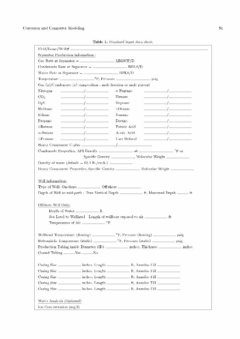
The model provides a physical description of whatis happening inside the production tubing as a functionof well depth. This type of description has been foundto be essential for an accurate prediction of corrosionrates in gas wells. Table 1 is a data sheet that presentsthe technical input into the model. Five categories ofminimum requirements for data input are mandatoryto successfully run the model. The minimum requireddata are:

� Completion information, such as true vertical depth,measured depth, size of tubing and casing data, isrequired.

� Temperature and pressure information at the sepa-rator wellhead and bottomhole is required.

� Separator production rates of the gas, condensateand oil are required.

� Analysis of the gas phase and gravity of the conden-sate are a minimum requirement for the input.

� A water analysis is needed if the in situ pH is tobe calculated. The model corrects the pH for thepresence of organic acid.

The required data, when used, is for a particulartime period in the life of the gas wells. Producinggas wells can have compositions and ow rates thatnormally change with time. This requires multiplemodeling of a gas well during its productive life toobtain the necessary picture for corrosion control. Themodel consists of �ve computer modules A, C, E, Fand G.

Computer module A calculates the temperatureand pressure pro�les in a well based on computermodule G, which produces the bottomhole owingtemperature for a given pressure drop as the gas exitsthrough the casing perforations into the well. Thephase behavior program which calculates the phasesthat exists at any point in the tubing is calculatedby computer module C. Information from computermodule C can help in deciding if the gas well tubing isoil wet or water wet. Computer module E is the owdynamic model that describes the type of ow regimespresent inside the well's tubing, and module F is themodel for corrosion rate prediction.

COMPUTER MODULES' PHYSICALDESCRIPTION

Physical Description Models

Models A and GThe �rst calculation made with the input data focuseson the temperature and pressure at each depth. Wellcon�guration, number and length of casing and thecasing �lls constitute the information necessary tocalculate the overall heat transfer coe�cient vs. depth.If the geothermal gradient is known, the heat transferrate can be determined. The uids inside the well are owing nonisothermally and a microscopic momentumand energy balance calculation on the owing gasproduces the equations necessary to calculate both thetemperature and pressure drop. Physical propertiesof the gas and liquids produced inside the tubingare permanently stored in the program for use whenneeded.

The gas undergoes a substantial pressure dropthrough the perforations during production. It ispossible to estimate the bottomhole owing temper-ature using Model G. This model accounts for theadiabatic expansion of the gas using the Peng-Robinsonequation of state. For a typical pressure drop, thetemperature of the gas can drop as much as 25�F fromits reservoir temperature value. Neglecting this factorcan signi�cantly a�ect the temperature pro�le and dewpoint location.

Model CSince a gas condensate well is being modeled, one mayexpect that in addition to gas, both condensate andwater could be present inside the tubing. Using theseparator production rates and the gas composition, itis possible for the Peng-Robinson EOS to predict thephases present at every depth. If a well is producingformation water, it can be said with certainty thatthe tubing contains water from the bottomhole to thewellhead. Otherwise, the water may show a dew pointsomewhere up the tubing. The program can predictthis water dew point location. Likewise, the location ofcondensate inside the tubing is equally important andthe model can predict the location of the condensateas well. Therefore, unlike oil wells which produce oilfrom bottomhole to wellhead, condensate wells may ormay not have condensate inside the tubing. Previouswork at the center [11] showed that approximately55% of condensate wells had no condensate inside thetubing, even though there was a substantial amount ofcondensate in the separator.

Model EOnce it has been established that there is liquid insidethe production tubing, it is important to know whattype of ow pattern exists at each depth. Figure 3


Table 1. Standard input data sheet.

Field/Lease/Well#

Separator Production Information :

Gas Rate at Separator = MMSCF/D

Condensate Rate at Separator = BBLS/D

Water Rate at Separator = BBLS/D

Temperature �F, Pressure psig

Gas (y)/Condensate (x) composition - mole fraction or mole percent

Nitrogen / n-Pentane /

CO2 / Hexane /

H2S / Heptane /

Methane / i-Octane /

Ethane / Nonane /

Propane / Decane /

i-Butane / Formic Acid /

n-Butane / Acetic Acid /

i-Pentane / User De�ned /

Heavy Component C plus /

Condensate Properties, API Gravity at �F or

Speci�c Gravity , Molecular Weight

Density of water (default = 62.4 lb./cu.ft.)

Heavy Component Properties, Speci�c Gravity , Molecular Weight

Well Information:

Type of Well: On-shore O�-shore

Depth of Well to mid-perfs : True Vertical Depth ft, Measured Depth ft

O�shore Well Only:

Depth of Water ft

Sea Level to Wellhead - Length of wellbore exposed to air ft

Temperature of Air �F

Wellhead Temperature ( owing) �F, Pressure ( owing) psig

Bottomhole Temperature (static) �F, Pressure (static) psig

Production Tubing inside Diameter (ID) inches, Thickness inches

Coated Tubing Yes No

Casing Size inches, Length ft, Annulus Fill





Water Analysis (Optional)

Ion Concentration (mg/l)


shows the �ve types of ow pattern that can existin vertical ow. Sixty percent of gas wells studiedusing Model E were found to be in annular ow atall points in the tubing. Of the remaining wells, 20%were found to be in mist ow at various points in thetubing and 20% were in churn-, slug- or bubble-type ow. A description of how the various ow regimes aremodeled follows.

Annular FlowThis type of ow is de�ned as having the bulk ofthe liquid owing upward against the pipe wall asa �lm. The gas phase is owing in the center ofthe pipe with some entrained liquid droplets in thegas phase. As described earlier [12], to obtain theliquid �lm thickness, it is necessary to calculate theentrained liquid. Then, using a microscopic momentumbalance on an element in gas-liquid two-phase ow, itis possible to develop a triangular relationship betweenpressure gradient, ow rate of liquid �lm and liquid�lm thickness [12].

Mist FlowIn high velocity wells, the corrosion rate can becomeactivation controlled due to a disturbance of the liquid�lm. This has been found to occur whenever (1)the annular ow program calculates that the liquid�lm is more than 50% turbulent, or (2) when theliquid droplets become large enough and of su�cientvelocity to disturb the liquid �lm. A paper byKocamustafaogullari et al. [13] gives an equation for themaximum stable droplet size, in terms of dimensionalgroups, such as liquid-and gas-phase Reynolds number,modi�ed Weber number and dimensionless physicalproperty groups. Using this concept, a paper [14]on the generation of droplets has shown that for gascondensate wells, the droplets are about 12 times largerin diameter than the thickness of the liquid �lm. Theirvelocities are somewhat less than that of the gas, but itis clear that these are high energy projectiles than canimpact the liquid �lm causing it to become increasinglyturbulent.

The ability to identify mist ow wells based ontheir abnormally high corrosion rates has been madepossible, using a discriminate analysis method [15]. Aprobability equation has been developed which usesfour parameters:

1. Mixture super�cial velocity.2. Reynolds number of liquid.3. Percent of liquid �lm in turbulent ow.4. Liquid pressure drop.

Based on this relationship, at every depth in an annular ow well, the equation is checked to determine if mist ow exists.

Slug/Churn/BubbleThe remaining 20% of gas wells exist in a ow patterndescribed as churn, slug or bubble. The approach usedin this work was based on considering the slug unit asconsisting of one Taylor bubble, its surrounding liquid�lm and a liquid pad between the bubbles. Severalimportant parameters, such as the length of the Taylorbubble and the average void fraction of the Taylorbubble and the slug unit were all calculated to within5 to 10% of the measured values. The void fraction ofthe slug unit is equivalent to the liquid holdup at eachpoint in the tubing.

This model has also proven to be useful in de�n-ing the slug/ churn transition point. Mashima andIshii [16] postulated that direct geometrical parame-ters, such as the void fraction are conceptually simplerand yet more reliable parameters to be used in owregime criteria than the traditional parameters such asgas and liquid super�cial velocities. With this in mind,other work [17] has shown that the vast majority of voidfractions for churn ow had a slug unit void fraction ofgreater than 0.73. None of the reported values below0.73 were in churn ow [18]. This parameter and itsvalue of 0.73 were selected in this work as the basis ofthe slug/churn transition point.

Corrosion Rate ModelSince a physical description of each ow regime hasbeen developed, attempts have been made to use these ow parameters to predict corrosion rates in thesewells. The following corrosion rate models have beendeveloped.

Annular FlowAs described previously, a well that is in the annular ow regime is usually found to exhibit a liquid �lmof a given thickness that can be divided into laminar,bu�er and turbulent components. Table 2 shows theresults of modeling 12 gas wells [12] that had knowncorrosion rates. The three wells with the thickest �lmfailed in the shortest period of time. From these data,an excellent tubing life correlation [12,19] based on the�rst principle, known as Model F, was developed, whichuses the �lm thickness and liquid velocity.

Mist FlowIf a well is found to be in mist ow by the pre-viously mentioned discriminate analysis equation, afundamental change is made to the above corrosionrate correlation. The velocity of the droplet is used inplace of the liquid velocity. In most cases, the dropletvelocity is within 90% of the gas velocity value. Thisapproach is theoretically more sensible, because it isbelieved by some investigators that the corrosion ratein mist ow is controlled by droplet impingement [20].The corrosion under this condition is believed to be


Table 2. Calculated �lm thickness in a gas condensate well.

Actual Life Entrainment Calculated Film Thickness (mils)

Well No. (months) % Laminar Bu�er Turbulent Total

1 44 0.21 1.0 5.0 0.4 6.5

2 117 1.04 0.5 1.6 . . . 2.1

3 113 0.28 1.2 3.5 . . . 4.7

4 59 0.60 0.5 2.4 . . . 3.0

5 71 0.25 1.0 4.5 . . . 5.5

6 116 0.62 0.8 2.9 . . . 3.6

7 62 0.49 1.0 4.4 . . . 5.4

8 91 0.63 1.5 4.2 . . . 5.7

9 97 0.26 1.3 4.1 . . . 5.5

10 32 0.27 1.2 6.1 3.8 11.1

11 41 0.33 0.8 3.8 2.1 6.7

12 66 0.14 1.1 5.0 . . . 6.2

partially activation and mass transfer controlled. Inother words, a protective iron carbonates �lm forms,which is then physically removed by impingement orby dissolution.

The accuracy of the two above-mentioned corro-sion rate correlations can be seen in Figure 5. Thetime to failure of 53 gas condensate wells that werein annular or mist ow has been shown to correlatewell with the �eld data [21]. The average percentdi�erence between predicted and actual corrosion rateswas �18%.

Slug FlowWhat has made this model comprehensive is inclusionof the physical description and corrosion prediction forthe nonannular ow regime. At this time, a total ofonly eight gas condensate wells in slug ow with knownproduction and corrosion rates have been documented.

Figure 5. USL model results compared to actualcorrosion.

All eight wells contained CO2 as the corrosion specie,and failed due to internal penetration. The wellswere found to be in slug ow at the depth of thefailure.

Corrosion rates in slug ow have been experimen-tally determined in the laboratory [22] to be higherthan churn ow.

It was decided to develop a correlation for slug ow wells by performing a regression on several ofthe calculated parameters [5]. The four parametersselected were (1) length of the Taylor bubble, (2)velocity of the Taylor bubble, (3) water rate, and (4)gas super�cial velocity. The resulting equation showedan average percent di�erence of �14% from the actualvalue.

To this date, no �eld data have been found for thecorrosion rate of churn ow wells. It is proposed thatthe same slug ow regression equation be used and thatan experimental factor be applied. The corrosion ratefor churn ow gas wells has been found experimentallyto be consistently 15% less than slug ow on theexperiments conducted [22]. Therefore, at the presenttime for churn ow wells, the slug parameters arecalculated and a 15% reduction factor is applied to theslug corrosion rate equation.

CONCLUSIONS

Pipeline Model

The pipeline computer model contains a physical de-scription of large diameter pipes with the modi�cationof the Dukler ow regime maps [23]. Within the ow regime area, the modeling of slug ow has been


the most di�cult ow regime to describe. A changein the calculation of the height of the liquid �lmhas given reasonable slug lengths and liquid hold upvalues.

The accurate prediction of the wettability of athree-phase of gas-oil-water is important for the deter-mination of the �nal corrosion rate. Describing \topof the line" corrosion in a condensing pipeline requiresan accurate calculation of the physical system, as wellas an accurate knowledge of the ow regime involved.The model is capable of determining if the \top of theline" corrosion can occur and what the pH value isat the top and bottom of the line. By incorporatingthe e�ect of organic acid in the calculations, it ispossible to predict how seriously it would a�ect thepipe.

Experimental data has veri�ed that, initially,the CO2 will dominate the corrosion process and asmall amount of H2S will contribute to an increasein corrosion. However, when the H2S species becomedominant, then, there is usually a drop in the corro-sion rate. Using the pitting model developed at ULLafayette, it has been possible to model the e�ect ofH2S on CO2 corrosion.

The pipeline model includes an internal risk as-sessment module. The risk assessment module is usedto calculate the probability of failure (pof) and providea risk classi�cation using a 1-5 rating (with 1 the best)as a function of years of use. From this information,a plot of risk classi�cation versus years, to determinethe expected time of failure, can be developed. Thee�ect of inhibitors on this classi�cation can also bedescribed. This pipeline program is the \state-of-art"computer model for predicting corrosion in pipelinesand owlines with the capability of risk assessment.This program has achieved accurate corrosion ratepredictions.

Oil Well Model

An updated computer model was developed that phys-ically describes owing or gas lifted vertical or deviatedwells. The model is capable of predicting temperature,pressure, phase behavior and ow dynamics at eachdepth inside a owing well. The ow regime has apronounced a�ect on the pressure drop and corrosionrate inside a well. It was found that the physicaldescription of the Taylor Bubble gave the best indi-cation of when the transition from slug to bubble owoccurred.

Corrosion rates in gas condensate wells correlatedwell to �ve physical parameters for vertical wells.These wells are believed to represent a higher corrosionrate than oil wells due to the inhibitive e�ect of thecrude. The expert system developed for oil wells usesthe factors of water cut, ow regime, temperature

and inhibitive e�ect to adjust the predicted corrosionrate.

The model was tested on several wells in the �eldand in these cases the predicted value of corrosion ratewas close to the actual corrosion rate.

Gas Well Model

A computer model has been developed for gas conden-sate wells and a number of conclusions can be made.

� The Corrosion Research Center at the University ofLouisiana at Lafayette has developed a computermodel which provides a comprehensive physicaldescription of gas wells.

� This physical description which includestemperature-pressure pro�le, phase behavior and ow dynamics can be useful in the design andproduction of these wells.

� The non-annular model completes the description ofthe �ve di�erent types of ow regime possible in agas well.

� The equations of Fernandes [10] are able not onlyto describe slug ow, but to provide a means bywhich the slug/churn transition and the bubble/slugtransition can be de�ned.

� The corrosion rates of wells operating in annular owhave been shown to be mass transfer controlled.

� Using a discriminate analysis method, the occur-rence of mist ow in a gas well can be predicted.

� Using the velocity of the droplets instead of theliquid velocity appears to provide a better estimateof corrosion rate in the mist ow regime.

� Model F which predicts the corrosion rate for annu-lar and mist type wells is accurate to within �18%.

� The same wells were shown to show no correlationbetween partial pressure of CO2 and the corrosionrate.

� Based on laboratory experiments, wells in slug oware 15% more corrosive than churn ow wells.

� Field data on nonannular ow wells show that theshorter the Taylor bubble, the more corrosive is thewell. This may be due to the washing e�ect of theslug.

� A statistical equation to predict the corrosion rateof nonannular gas wells has been developed, whichhas an accuracy of �14%.

REFERENCES

1. Farshad, F.F. and Rieke, H.H. \Gas well optimiza-tion: A surface roughness approach", CI/PC/SPEGas Technology Symposium Joint Conference, Calgary,Alberta, Canada, p. 8 (2008).


2. Chillingar, G.V., Mourhatch, R. and Al-Qahtani,G.D., The Fundamentals of Corrosion and Scaling,Gulf Publ. Company, Houston, TX, p. 276 (2008).

3. Chillingar, G.V. and Beeson, C.M. \Surface operationsin petroleum production", American Elsevier, NewYork, NY, p. 397 (1969).

4. Garber, J.D., Farshad, F.F. and Reinhart, J.R. \Amodel for predicting corrosion rates on oil wells con-taining carbon dioxide", SPE/EPA/DOE Explorationand Production Environment Conference, San Anto-nio, TX, p. 21 (2001).

5. Garber, J.D., Polaki, V., Varansi, N.R. and Adams,C.D. \Modeling corrosion rates in non-annular gascondensate wells containing CO2", NACE AnnualMeeting, p. 53 (1998).

6. Farshad, F.F., Garber, J.D. and Polaki, V. \A com-prehensive model for predicting corrosion rates in gaswell containing CO2", SPE Prod. and Facilities, 15(3),pp. 183-190 (2000).

7. Garber, J.D., Farshad, F.F., Reinhart, J.R., Hui Liand Kwei Meng Yup \Prediction pipeline corrosion",Pipeline and Gas Technology, 7(11), pp. 36-41 (2008).

8. Farshad, F.F., Garber, J.D. and Lorde, J.N. \Predict-ing temperature pro�le in producing oil wells usingarti�cial neural network", SPE Sixth Latin Ameri-can and Caribbean Petroleum Engineering Conference,Caracas, Venezuela (1999).

9. Koch, G.H., Brongers, M.P.H., Thompson, N.G.,Virmani, Y.P. and Payer, J.H., Corrosion Costs andPreventive Strategies in the United States, PublicationNo. FHWA-RD-01-156:1-11 (2002).

10. Fernandes, C.S. \Experimental and theoretical stud-ies of isothermal upwards gas-liquid ows in verticaltubes", University of Houston, Houston, PhD Disser-tation (1981).

11. Garber, J.D., Adams, C.D. and Hill, A.G. \Expertsystem for predicting tubing life in the gas condensatewells", NACE Annual Meeting, p. 273 (1992).

12. Fang, C.S., Garber, J.D., Perkins, R.S. and Reinhardt,J.R. \Computer model of a gas condensate well con-taining CO2", NACE Annual Meeting, p. 465 (1989).

13. Kocamustafaogullari, G., Smits, S.R. and Razi, J., Int.J. Heat Mass Transf., 37, p. 955 (1994).

14. Garber, J.D., Singh, R., Rama, A. and Adams, C.D.\An examination of various parameters which produceerosional conditions in gas condensate wells", NACEAnnual Meeting, p. 132 (1995).

15. Garber, J.D., Walters, F.H., Singh, C., Alapati, R.R.and Adams, C.D. \Downhole parameters to predicttubing life and mist ow in gas condensate wells",NACE Annual Meeting, p. 25 (1994).

16. Mashima, K. and Ishii, M. \Flow regime transitioncriteria for upward two-phase ow in vertical tubes",Int. J. Heat Mass Transf., 27, p. 723 (1984).

17. Garber, J.D. and Varanasi, N.R.S. \Modeling non-annular ow in gas condensate wells containing CO2",NACE Annual Meeting, p. 605 (1997).

18. Fernandes, R.C., Semiat, R. and Dukler, A.E. \Hy-drodynamic model for gas-liquid slug ow in verticaltube", Am. Inst. Chem. Eng. J., 29, p. 981 (1983).

19. Perkins, R.S., Garber, J.D., Fang, C.S. and Singh,R.K. \A procedure for predicting tubing life in annular ow gas condensate wells containing carbon dioxide",Corrosion, 52(10), p. 801 (1996).

20. Smart, J.S. \The meaning of the API-RP14E formulafor erosion corrosion in oil and gas production", NACEAnnual Meeting, p. 468 (1991).

21. Adams, C.D. et al. \Computer modeling to predictcorrosion rates in gas condensate wells containingCO2", NACE Annual Meeting, p. 31 (1996).

22. Varanasi, N.R.S. \Modeling nonannular ow in gascondensate wells", MS dissertation, University ofSouthwestern Louisiana, Lafayette, Louisiana (1996).

23. Dukler, A.E., Wicks, M. III. and Cleveland, R.G.\Friction pressure drop in two-phase ow: an approachthrough similar uid mechanics and heat transfer invertical falling-�lm system", Chem. Eng. Prog. Sym-posium Series, 56(30), p. 1 (1964).

BIOGRAPHIES

Fred F. Farshad holds a PhD degree in PetroleumEngineering from the University of Oklahoma. He isnow a Chevron-Texaco Endowed Research Professorin the Department of Chemical Engineering at theUniversity of Louisiana at Lafayette, where he wasawarded the university's 1999 Outstanding FacultyAward for teaching. He is also a member of theRussian Academy of Natural Sciences. He previouslyworked for Cities Service Oil Co. and Core Labo-ratories. Professor Farshad established and set upthe Pipe Surface Roughness Testing and Fluid FlowLaboratory Facility at the University of Louisianaand is internationally renowned as the originator ofresearch on the surface roughness of newly developedpipes using pro�ling instruments. He has served onnumerous SPE technical committees, authored over75 technical papers and lectured and conducted shortcourses worldwide.

James D. Garber received his BS degree from theUniversity of Louisiana at Lafayette, and MS and PhDdegrees from the Georgia Institute of Technology inChemical Engineering. He is Professor and Head of theChemical Engineering Department at the Universityof Louisiana at Lafayette and the Director of theUL Lafayette Corrosion Research Center. For thepast 28 years, he has been a registered professionalengineer and NACE member. He performs FailureAnalysis through his company, `Garber Laboratoriesof Lafayette', Louisiana.

Herman H. Rieke, PhD, has multiple degrees inGeology and Petroleum Engineering from the uni-


versities of Kentucky and Southern California, andhas served the academic, industrial and governmentalsectors in The United States of America and inter-nationally. He has recently completed his tenure asHead of the Department of Petroleum Engineeringat The University of Louisiana at Lafayette, USA,and presently has dual appointments as Professorin the Departments of Petroleum Engineering andGeology. He is a foreign member of the RussianAcademy of Natural Science and the National Academyof Engineering of Armenia. Some of his recent majorawards include: the Einstein Medal (American Sectionof the Russian Academy of Natural Sciences, 2001)Kapitsa Gold Medal (Russian Academy of Natural

Sciences, 1996), Honorary Doctor of Science Degreefrom the All Russia Petroleum Scienti�c ResearchGeological Exploration Institute (VNIGRI), 1996, andProfessor Honoris Causa (Dubna International Uni-versity, Russia), 1996. He has published 120 jour-nal articles and is author/editor of nine technicalbooks.

Shiva Guru Komaravelly received his MS degreefrom the Department of Chemical Engineering at theUniversity of Louisiana at Lafayette. He works on thesurface roughness of pipes at the Surface RoughnessTesting and Fluid Flow Laboratory facility at theUniversity of Louisiana.

prefouling behavior of particles in petroleum flow...

Documents